Embed Size (px)
Citation preview

Full Terms & Conditions of access and use can be found athttps://www.tandfonline.com/action/journalInformation?journalCode=hsem20
Structural Equation Modeling: A Multidisciplinary Journal
ISSN: (Print) (Online) Journal homepage: https://www.tandfonline.com/loi/hsem20
Multilevel Modeling in the ‘Wide Format’ Approachwith Discrete Data: A Solution for Small ClusterSizes
M.T. Barendse & Y. Rosseel
To cite this article: M.T. Barendse & Y. Rosseel (2020) Multilevel Modeling in the ‘Wide Format’Approach with Discrete Data: A Solution for Small Cluster Sizes, Structural Equation Modeling: AMultidisciplinary Journal, 27:5, 696-721, DOI: 10.1080/10705511.2019.1689366
To link to this article: https://doi.org/10.1080/10705511.2019.1689366
View supplementary material
Published online: 03 Jan 2020.
Submit your article to this journal
Article views: 235
View related articles
View Crossmark data
Multilevel Modeling in the ‘Wide Format’ Approachwith Discrete Data: A Solution for Small Cluster Sizes
M.T. Barendse and Y. RosseelGhent University
In multilevel data, units at level 1 are nested in clusters at level 2, which in turn may benested in even larger clusters at level 3, and so on. For continuous data, several authorshave shown how to model multilevel data in a ‘wide’ or ‘multivariate’ format approach. Weprovide a general framework to analyze random intercept multilevel SEM in the ‘wideformat’ (WF) and extend this approach for discrete data. In a simulation study, we varyresponse scale (binary, four response options), covariate presence (no, between-level,within-level), design (balanced, unbalanced), model misspecification (present, not present),and the number of clusters (small, large) to determine accuracy and efficiency of theestimated model parameters. With a small number of observations in a cluster, resultsindicate that the WF approach is a preferable approach to estimate multilevel data withdiscrete response options.
Keywords: Discrete data, multilevel, structural equation modeling, random intercepts
INTRODUCTION
Structural equation modeling (SEM) is a flexible and powerfulframework to analyze the interrelationships between manyobserved and latent variables (seeBollen, 1989). The popularityof SEM is a striking feature of quantitative research in the socialsciences (see Guo, Perron, & Gillespie, 2008; MacCallum &Austin, 2000; Yang, 2018). Throughout the years, the SEMframework has been extended to analyze discrete responseoptions, such as binary- or four-point response scales (seeJöreskog & Moustaki, 2001; Wirth & Edwards, 2007) or datafrom a hierarchical ormultilevel structure, such as employees inteams, patients from different doctors, or students in schools(see Hox, Moerbeek, & Van de Schoot, 2017). However, realdata are evenmore complex and often contain a combination ofmultilevel structures and discrete response options. This callsfor more sophisticated estimation techniques.
Three estimation methods have been suggested in theliterature for analyzing multilevel SEM data with discreteresponse options: (1) marginal maximum likelihood (MML;
see Hedeker & Gibbons, 1994), (2) Bayesian estimation (e.g.,Fox, 2010), and, (3) the multilevel (weighted) least squaresestimation method (Asparouhov & Muthén, 2007).Unfortunately, both MML and Bayesian estimation are com-putationally very intensive, limiting their practical use (seeFox, 2010; Jöreskog & Moustaki, 2001; Wirth & Edwards,2007). The multilevel (weighted) least squares method canhandle many more latent variables, but has not been thor-oughly studied and showed mixed results in simulation stu-dies (Asparouhov & Muthén, 2007; Depaoli & Clifton, 2015;Holtmann, Koch, Lochner, & Eid, 2016).
As analyzing multilevel data with discrete responseoptions is complex, researchers often turn to suboptimalanalyzes techniques, such as using sum-scores or ignoringeither the multilevel or discrete nature of the data (see forexample Koomen, Verschueren, van Schooten, Jak, &Pianta, 2012; Lee, 2009; Li, Fortner, & Lei, 2015). Thisis unfortunate as this may jeopardize the results of theanalysis and therefore any decision-making based on theseresults. Currently lacking are statistical techniques thatoffer an efficient and practical method to analyze multileveldatasets with discrete response scales.
In this article, we propose a solution for discrete multi-level data with a small number of observations in a cluster(approximately < 10). The National Longitudinal Study of
Correspondence should be addressed to M. T. Barendse. Email:[email protected]
Supplemental data for this article can be accessed here.
Structural Equation Modeling: A Multidisciplinary Journal, 27: 696–721, 2020© 2019 Taylor & Francis Group, LLCISSN: 1070-5511 print / 1532-8007 onlineDOI: https://doi.org/10.1080/10705511.2019.1689366

Adolescent Health (NLSAH, 2005) data is an example ofa dataset with small cluster sizes, where at each wave15,000 adolescents are nested in approximately 2,600neighborhoods (i.e, about six per cluster). On a smallerscale, among others, Koomen, Verschueren, and Pianta(2007) collected data in Dutch primary schools with onaverage two to three children in each class. To analyzethese type of data, we will use the so called ‘wide format’(WF) approach. Using different model specifications, theWF approach is discussed in the SEM literature for con-tinuous multilevel data by Bauer (2003), Curran (2003),and Mehta and Neale (2005). In the WF approach, dataare arranged in such a way that each data row correspondsto a single cluster. The multilevel structure is then explicitlymodeled as will be explained in section “Multilevel SEM inthe WF Approach” and section “WF Approach withDiscrete Data.” The WF approach differs from the generalway multilevel data are organized and modeled, in thisarticle referred to as the ‘long format’ (LF) approach. Inthis LF approach each row corresponds to the data ofa single unit, and many rows constitute a single cluster.Dealing with discrete data using the WF approach yieldssome additional advantages over the LF approach. First, theWF can handle multilevel data using single-levelsoftware. Second, the multilevel model is explicitly mod-eled and therefore offers freedom to freely estimate para-meters that are restricted in the LF approach.
The goal of this paper is twofold: (1) to offer a generalfrequentist framework to analyze random intercept multileveldata in the WF approach and (2) to extent and test the WFapproach for discrete data. The former goal is necessary asdifferent aspects of the WF approach, like the inclusion ofcovariates, obtaining test statistics, dealing with unbalanceddata, and handling missing data have been described separatelyin the literature; either in the context of generalized linear mixedmodels (e.g., Croon&vanVeldhoven, 2007), or in the context ofWF multilevel models with different specifications (e.g., Bauer,2003; Curran, 2003; Mehta & Neale, 2005). This fragmentedliterature has not been united to a generalWF framework. To thebest of our knowledge, an extension of the WF approach todiscrete data has not been investigated yet. As will be explainedin section “WFApproachwithDiscrete Data” and the illustrativeexample, the WF approach turns out to be much more compu-tationally efficient compared to the often used MML estimationmethod in the LF approach. Using the WF approach does notrequire specialized multilevel software, which decreases thecomplexity of estimating multilevel models.
The paper is organized as follows: First, a brief over-view of single level SEM and multilevel SEM for contin-uous and discrete data is given. Next, we will describe theWF approach for continuous and discrete data. Thereafter,we will perform a simulation study to evaluate the generalWF framework and to compare several WF estimationmethods to LF estimation methods in terms of the accuracy
and efficiency of the parameter estimates under differentconditions. Finally, the use of the WF approach for discretedata will be illustrated by means of an application ineducational research on student-teacher relationships.
Single-level SEM
Continuous Data
The measurement equation and the structural equationare the two fundamental equations that define the generalSEM framework. The measurement equation equals
y ¼ νþ Ληþ ε; (1)
where y is a p� 1 vector of observed variables, ν is a p� 1vector of intercepts, Λ is a p� m matrix of factor loadingsrelating the p observed variables to the m latent variables, ηis a m� 1 vector of latent variable scores, and ε is a p� 1vector of residuals. The structural equation equals
η ¼ αþ Bηþ ζ ; (2)
where α is a m� 1 vector of latent factor means andintercepts, B is a m� m matrix of regression coefficientsamong the latent factors, and ζ is a m� 1 vector of resi-duals. In SEM we assume that Covðε; ζÞ = 0, Covðη; εÞ = 0,Covðη; ζÞ = 0, EðεÞ = 0, EðζÞ= 0, diagðBÞ = 0, and thatðI� BÞ is invertible, where I is a m� m identity matrix.Using covariance algebra we can find expressions for thecovariance and the mean structure of y, denoted by Σ andμ. The p� p covariance matrix Σ of y is expressed asa function of the model parameters (θ) and equals
ΣðθÞ ¼ ΛðI� BÞ�1ΨðI� BÞ�1TΛT þΘ (3)
where variances and covariances of η and ε are denoted byΨ and Θ. The mean structure implied by Equation 1 andEquation 2 equals
μðθÞ ¼ νþ ΛðI� BÞ�1α: (4)
Assuming multivariate normality, the model parameters (θ)can be estimated via maximizing the likelihood, or equiva-lently, by minimizing the following objective function:
FML ¼ flnjΣðθÞj � lnjSj þ tr½ΣðθÞ�1S� � pgþ f½�y� μðθÞ�TΣðθÞ�1½�y� μðθÞ�g; (5)
where S is the sample covariance matrix and �y is theobserved mean vector. Under the assumptions of multivari-ate normality, a large enough sample size and a correctmodel specification yields unbiased parameter estimates(Bollen, 1989). Alternative estimators are the generalized
MULTILEVEL MODELING IN THE ‘WIDE FORMAT’ APPROACH WITH DISCRETE DATA 697

least squares and the weighted least squares (see Bollen,1989; Browne, 1995; Jöreskog, 1981).
Discrete Data
Items are often scored with binary codings or three- orfour-point scales. To deal with these discrete data,a distinction is made in the SEM literature between limitedinformation estimation methods that use only summaries ofthe data and full information estimation methods that useall available information in the data.
Limited Information Estimation Methods. The leastsquares estimation methods and the pairwise maximumlikelihood (PML) estimation method are both limited infor-mation methods that use only summaries of the data. Thesemethods, mostly developed within the SEM literature,assume underlying continuous latent response variables.A variable yik for a certain individual on item k with Ck
response scales stems from an underlying continuous vari-able y�ik with a normal distribution Nðy�ikj0; σ2k) and τkcvalues that refer to thresholds
yik ¼ c , τk;c�1 <y�ik < τk;c (6)
for categories ck ¼ 1; 2; . . . ;Ck , with τk;0 ¼ �1 andτk;C ¼ þ1.
Least Squares Estimation Methods. The threestage weighted least squares method is often applied toestimate models for large datasets with discrete data. Inthe first stage, the thresholds are estimated using the uni-variate data. In the second stage, the pðp� 1Þ=2 polychoriccorrelations are estimated (see Olsson, 1979; Olsson,Drasgow, & Dorans, 1982). In the third stage, the modelparameters are estimated using the weighted least squaresestimation method;
FWLS ¼ ðs� σ̂Þ0 W�1ðs� σ̂Þ; (7)
where s denotes a vector with non-redundant sample-basedstatistics, σ̂ denotes a vector with the non-redundant model-based statistics (i.e., thresholds and polychoric correla-tions), and W�1 denotes the inverse of a weight matrixthat estimates the asymptotic covariance matrix of
ffiffiffiffiIs
p(see Muthén & Satorra, 1995), where I denotes the samplesize. In the least squares framework (see Browne, 1984;Muthén, Du Toit, & Spisic, 1997), there are three differentchoices for W, leading to WLS using the full weight matrixW, DWLS using only the diagonal of W, and ULS whereW is replaced by the identity matrix (I).
Pairwise Maximum Likelihood Estimation Method.The single level PML estimation method was introduced inthe SEM framework by Jöreskog andMoustaki (2001). In this
estimation method, the complex likelihood is broken down asa product of bivariate (and sometimes univariate) likelihoodswhich are computationally easier to handle. The PMLestimation method is part of a broader framework ofcomposite ML estimators which are asymptotically unbiased,consistent, and normally distributed (see Lindsay, 1988;Varin, 2008). In PML, the log-likelihood contribution ofa single observation is a sum of p? ¼ pðp� 1Þ=2 compo-nents, each component being the bivariate log-likelihood oftwo variables (i.e., k and l):
log li ¼Xp�1
k¼1
Xpl¼kþ1
½log f ðyik; yil; θÞ�
¼Xk<1
½log f ðyik; yil; θÞ�: (8)
Given a random sample Y ¼ fy1; y2; :::yIg of size I, the totallog-likelihood of the data is the sum of all individualcontributions:
log Lðθ;YÞ ¼XI
i¼1
log li: (9)
In principle Equation 8 is general and can deal with any type ofdata (continuous or discrete, and combinations thereof). Untilnow, the PML estimation method in the SEM context has onlybeen applied with discrete data. For discrete indicators k and l,the exact form of f ðyik ; yil; θÞ in Equation 8 is:
log f ðyik; yil; θÞ ¼XCk
a¼1
XCl
b¼1Iðyik ¼ a; yil ¼ bÞ
logωðyik ¼ a; yil ¼ bÞ; θÞ;(10)
where
ωðyik ¼ a; yil ¼ b; θÞ ¼ðτk;aτk;a�1
ðτl;bτl;b�1
f ðy�ik; y�il; θÞdy�ikdy�il;
¼ ϕ2ðτk;a; τl;b; ρklÞ� ϕ2ðτk;a�1; τl;b; ρklÞ� ϕ2ðτk;a; τl;b�1; ρklÞþ ϕ2ðτk;a�1; τl;b�1; ρklÞ;
(11)
where ρkl denotes the model implied correlation between y�ikand y�il, and ϕ2ðτ1; τ2; ρÞ denotes the bivariate cummulativenormal distribution with correlation ρ evaluated at pointðτ1; τ2Þ. The PML estimator produces unbiased results(see Katsikatsou, Moustaki, Yang-Wallentin, & Jöreskog,2012).
698 BARENDSE AND ROSSEEL
Scaling with Discrete Data. With discrete data, weneed to determine a metric for y�. A common way is to usethe delta parameterization where Θ is not a free parameter,but given by
Θ ¼ Δ�2 � diagðΣ�Þ (12)
where Σ� equals ΛðI� BÞ�1ΨðI� BÞ�1TΛT with the scal-ing factors defined as
Δ ¼ diagðΣ�Þ�1=2: (13)
Alternatively, the theta parameterization can be chosen.Here the diagonal of Θ is an identity matrix and the scalingfactors (Δ) are obtained as:
Δ�2 ¼ diagðΣ�Þ þΘ: (14)
Full Information Estimation Method. An often usedfull information estimation method is the marginal maxi-mum likelihood (MML), as described by Bock and Aitkin(1981). This estimation method has been developed withinthe item response theory literature and integrates over thedistribution of the latent variables. The log-likelihood forthe data (i.e., Y) can be written as the sum of all of the log-likelihoods for all individuals i:
logLðθ;YÞ ¼XI
i¼1
log li
¼XI
i¼1
log fiðyi; θy; θηÞ (15)
where the individual likelihood contribution of observationi equals
li ¼ðDðηÞ
f ðyijη; θyÞgðη; θηÞdη
¼ðDðηÞ
Ypk¼1
fikðyikjη; θyÞgðη; θηÞdη (16)
and where DðηÞ is the domain of integration and gð�Þ is theprior density of η. The MML estimation method is compu-tationally very intensive as it has to integrate out the latentvariables using numerical integration (i.e., Gauss-Hermitequadrature, adaptive quadrature, Laplace approximation, orMonte Carlo integration). This estimation method can be
applied with different link functions (e.g., probit, logit, log,logistic, and complementary log-log).
Multilevel SEM in the LF Approach
From the late 1980’s, the SEM framework started to incor-porate features from multilevel regression (e.g., Bryk &Raudenbush, 1987). Schmidt (1969) was the first todescribe a saturated model of a within-covariance matrix(i.e., individual deviations from the group mean) anda between-covariance matrix (i.e., group means) forbalanced data. His work was further developed byGoldstein and McDonald (1988), McDonald andGoldstein (1989), Muthén (1989, 1990), and McDonald(1993). More recently, estimation methods to analyze mul-tilevel discrete data were developed. Multilevel SEM in theLF approach is the standard way to model multilevel datawhere the data is organized in such a way that each rowcorresponds to a single unit.
Continuous Data
Here, we will describe the multilevel model as intro-duced by McDonald and Goldstein (1989) with a slightlyadjusted mean structure. In a two-level set-up, the multi-variate response vector yji can be decomposed in a betweenpart uj and a within part uji
yji ¼ uj þ uji; (17)
where j ¼ 1; . . . ; J is an index for the clusters, and i ¼1; . . . ; Ij is an index for the units within a cluster. As ujand uji are independent, the expected value equals
EðyjiÞ ¼ μb þ μw; (18)
where μw is only needed if there are variables that onlyexist at the within-level. The covariance can be decom-posed as
CovðyÞ ¼ ΣT ¼ Σb þ Σw: (19)
On both the within-level (Σw, μw) and the between-level(Σb, μb) a different model can be fitted. Consider data froma single cluster with z representing variables at thebetween-level:
vj ¼ ½zj; yj1; yj2 . . . yjIj �T ; (20)
with the following expectation of vj
E½vj� ¼ vj ¼ ½zj; yj�T ¼ ½zj; yj1; yj2 . . . yjIj �T : (21)
The covariance matrix, referred to as VjðθÞ, can be writtenas:
MULTILEVEL MODELING IN THE ‘WIDE FORMAT’ APPROACH WITH DISCRETE DATA 699

Cov½vj� ¼ VjðθÞ ¼ Σzz 1TIj � Σzy
1Ij � Σyz Σyy
� �: (22)
with Σzz ¼ Covðzj; zjÞ, Σzy ¼ Covðzj; yjÞ, andΣyy ¼ IIj � ΣwðθÞ þ 1Ij1
TIj� ΣbðθÞ. Assuming multivari-
ate normality, the model parameters in θ can be estimatedvia minimizing the ML objective function which equalsminus two times the log–likelihood function withouta constant over all clusters:
FML ¼XJj¼1
lnjVjj þ ðvj � vjÞTV�1j ðvj � vjÞ: (23)
As Vj can become quite large, several methods are used tofind expressions to compute V�1
j and Vj
�� �� efficiently (see
McDonald & Goldstein, 1989).
Discrete Data
Some estimation methods for single level discrete datacan be applied in the multilevel context. As multilevel datahas a more complex structure, adjustments to the algo-rithms have to be made.
Limited Information Estimation Methods. Due tothe work of Asparouhov and Muthén (2007) the leastsquares estimation methods can be applied to discrete mul-tilevel data. For the discrete variable k for individual i incluster j, the threshold parameters are now defined by
yijk ¼ c , τk;c�1<y�ijk<τk;c (24)
The underlying variable y�ij is decomposed into a between-level (ubj; i.e., random intercept) and a within-level (uwij)part:
y�ij ¼ uwij þ ubj: (25)
A separate structural model can now be defined at bothlevels. The least squares estimation methods for multileveldata in the LF approach are based on the single level leastsquares estimation methods. In the first stage, the thresh-olds are estimated using an univariate model with the two-level maximum likelihood estimation method (Asparouhov& Muthén, 2007). In the second stage, polychoric correla-tions are estimated based on bivariate models by fixing theunivariate parameters to their first stage estimates(Asparouhov & Muthén, 2007). Minimizing the fit functionwith respect to the parameters of the model at both levelswith Equation 7, is the last stage of the estimation process.
Full Information Estimation Method. The LFMML, as described by Hedeker and Gibbons (1994)and Rabe-Hesketh, Skrondal, and Pickles (2004a), is
based on the MML for single level data (Bock &Aitkin, 1981). In the multilevel context, the randomintercept can be written as a vector of latent variables,referred to as ηy, so that the extended set of latentvariables equals η� ¼ (η,ηy). This formula can beextended to models with more latent variables at differ-ent levels of the multilevel model. For a two level model,the log-likelihood for the data can be written as the sumof the log-likelihoods of all the clusters j:
log Lðθ;YÞ ¼XJj¼1
log lj
¼XJj¼1
log fjðyj; θy; θη� Þ(26)
where the individual likelihood contribution of cluster jequals
lj ¼ðDðη�Þ
f ðyjjη�; θyÞgðη�; θη� Þdη�
¼ðDðη�Þ
Ypk¼1
fjkðyjkjη�; θyÞgðη�; θη� Þdη�(27)
where Dðη�Þ is the domain of integration and gð�Þ is theprior density of η�. The multilevel MML estimation methodis very flexible and can be extended with more levels,covariates, different link functions (e.g., probit, logit, log,logistic, and complementary log-log), and random slopes(see Rabe-Hesketh et al., 2004a). Unfortunately, the MMLestimation technique for multilevel data is computationallyeven more intensive than the single level MML estimationmethod. To reduce the number of latent variables in two-level factor models, the residuals at the between-level areusually not estimated by default (e.g., Muthén & Muthén,2010; Rabe-Hesketh, Skrondal, & Pickles, 2004b).
Multilevel SEM in the WF Approach
As an alternative to the above described LF approach to fitmultilevel data, one can use a WF approach. In this WFapproach, the multilevel model is explicitly modeled andthe data is restructured such that all units in a cluster arestored in a single row. Despite several papers describing theWF approach, this approach is seldom applied. Below weoffer a general framework to fit multilevel data witha random intercept in the WF approach for both continuousand discrete data.
Continuous Data
McArdle and Epstein (1987) were the first authors whoshowed how multilevel models of individual change can befitted using a mean and covariance structure analysis with
700 BARENDSE AND ROSSEEL

time-structured data in latent growth curve models (see alsoChou, Bentler, & Pentz, 1998; MacCallum, Kim, Malarkey,& Kiecolt-Glaser, 1997; Meredith & Tisak, 1990; Willett &Sayer, 1994). The latent growth curve models becomeconfirmatory factor analysis (CFA) models with modelparameters fixed to specific data values. A random-intercept multilevel model can then be estimated asa restricted CFA model, where univariate multilevel modelsbecome multivariate uni–level models. In this way, eachdata row consists of all observations in a cluster with latentvariables constructed from unit-specific versions of thevariables. Figure 1 shows data, a graphical representation,and a formula of a random intercept model in both the LFapproach and the WF approach.
Later, Curran (2003) and Bauer (2003) further devel-oped the WF approach and provided examples of multilevelSEM using the WF approach. Curran extended the growthcurve model with more SEM related options, such as ran-dom intercepts and slopes, and latent or observed covariatesat the between-level. Bauer estimated random interceptmodels including level-2 predictors and structural relationsbetween latent variables. He also reflected on the use offormal tests of model fit and demonstrated the applicabilityof multilevel SEM with unbalanced data. In 2005, Mehtaand Neale provided a more extended framework for mod-eling multilevel models in the WF approach with
continuous data, where person-specific data is used formodeling means as well as covariances at an individuallevel. The main difference between the representation ofMehta and Neale and Bauer and Curran is that the modelsof Mehta and Neale impose restrictions on the covariancematrix in such a way that the model is decomposed intoa between–level and a within–level that allows for differentstructures and parameter values at different levels.
In this paper, we will continue with the model of Mehtaand Neale (2005) that explicitly models the multilevelmodel of McDonald and Goldstein (1989). To deal withcontinuous data in the WF approach, we proceed with thefollowing steps:
1. Rearrange the data in such a way that each rowcorresponds to a single cluster (see data in Figure 1).
2. Construct a model at the within-level involving thevariables that belong to a single unit in a cluster andrepeat this model as many times as the maximumcluster size.
3. Put equality constraints on all parameters across unitsin a cluster. For example, in a one factor model,equality constraints are necessary on the factor load-ings, factor variances, and error variances. If vari-ables are both at the within- and the between-level,
1a: LF approach> longDatay clus2.416245 12.189816 11.868216 11.064450 13.915011 22.284573 2
-0.041089 22.034896 2... ...
y
y
Between
Within
yij = β0 + b0j + εij
1b: WF approach
> D.widey1 y2 y3 y42.416245 2.189816 1.868216 1.0644503.915011 2.284573 -0.041089 2.034896... ... ... ...
ηy
y1 y2 y3 y4
1 1 1 1
Between
Within
yj = β0 + εj
FIGURE 1 A random intercept model with the corresponding data, figure and formula in both the LF (left hand side)- and WF -approach (right hand side).Note: The rounded boxes represent the within- and between versions of the original variable y for four units per cluster. ηy corresponds to the unit-specificversion of y on the between level, which equals a factor with loadings fixed at unity. Residual variances (not shown here) contain equality restrictions toensure only one residual variance is estimated.
MULTILEVEL MODELING IN THE ‘WIDE FORMAT’ APPROACH WITH DISCRETE DATA 701

the intercepts at the within-level should be fixed tozero.
4. For each endogenous variable at the within-level,construct a latent variable where the indicators cor-respond to the unit-specific version of that variable;The factor loadings are fixed to one; These latentvariables represent the random intercepts of thesevariables in the model.
5. Construct a model at the between-level with thenewly constructed between-level latent variables.
Figure 2 shows a one factor model according to the para-meterization of Mehta and Neale (2005) for the case wherewe have three units in each cluster. The within factor isreferred to as ηfw, the unit-specific version of the variableson the between-level is referred to as ηy, and the betweenfactor is referred to as ηfb. To clarify the proposed steps, wegive the lavaan syntax corresponding to Figure 2 inAppendix A. The figure shows that the WF approach ismore flexible than the LF approach, as the equality restric-tions across units in a cluster (e.g., e to h for the factorloadings and/or i to l for the residual variances in Figure 2)can all be tested by freeing the restrictions in the WF
approach. Note that within the LF approach, it is notpossible to free restrictions across clusters. Below we willdescribe how to extent the framework of Mehta and Neale(2005) and deal with covariates, missing data, and obtain fitstatistics.
WF Approach with a Covariate. The WF multilevelmodel can be extended with covariates at the within- and/orthe between-level (see Croon and van Veldhoven (2007) foradding covariates in a WF multilevel regression model).Values for the between-level covariate are equal for allunits in a cluster and can be added to the model. The effectof the between-covariate is calculated by regressing therandom intercept on the covariate. Values for the within-level covariate are unique for each individual in a cluster.The effect of the within-covariate is calculated by regres-sing the observed variables at the within-level on the cov-ariates with equality restrictions. As the within-levelcovariate contains equality restrictions, they are consideredstochastic and jointly modeled with the other variables asendogenous variables.
Lüdtke et al. (2008) describe multilevel models witha covariate that exists both at the within- and the between-
y1.2 y2.2 y3.2 y4.2 y1.3 y2.3 y3.3 y4.3y4.1y3.1y2.1y1.1
ηy3ηy4
ηy1ηy2
ηfb
1 11 1 1 1 1
1 11
1 1
a b dc
ηfw(2)ηfw(1) ηfw(3)
e f g h e f g h e f g h
Between
Within
FIGURE 2 One factor multilevel CFA model in the WF approach (four variables with three units per cluster). Note: The rounded boxes represent thewithin- and between versions of the original variables y1:1 to y4:3 for three units per cluster. ηy1 to ηy4 correspond to the unit-specific version of that variableon the between level, where labels a to d reflect the between-level factor loadings. For identification purposes, one factor loading or the variance of ηfb mustbe fixed to unity. The structures below y1:1 to y4:3 account for the within–level latent variables (i.e., ηfwð1Þ to ηfwð3Þ) with parameter labels e to h for the factor
loadings. For identification purposes, one factor loading of each within factor (ηfw) or the variance of ηfw must be fixed to unity. Identical parameter labelsindicate equality constraints in the model. Residual variances (not shown here) also contain equality restrictions (i.e., i to l). Appendix A shows thecorresponding lavaan syntax.
702 BARENDSE AND ROSSEEL

level in the LF approach. One can then either aggregate thecovariate before the analysis to get between-level values forthe covariate, referred to as the multilevel manifest covari-ate approach, or split the covariate in a within anda between part, referred to as the multilevel latent covariateapproach. Figure 3a shows the MMC approach in WFapproach and Figure 3b shows the MLC approach in the‘wide format approach. To obtain the correct between-leveleffect in Figure 3b, one has to calculate the so called“contextual effect” by estimating the between–level effect(i.e., b) and subtract this from the within-level effect (i.e.,a). Appendix B shows the lavaan syntax that can be addedto Appendix A to fit a model with a covariate on both thewithin- and the between-level.
Missingness in the WF Approach. In the multilevelSEM setting, we make a distinction between design miss-ingness and within cluster missingness. Design missingnessoccurs with an unbalanced multilevel design, where thecluster sizes differ. In the WF approach the cluster with
the largest number of units determines the width of thedataset and all other clusters with less units have missingvalues (see Bauer, 2003). With cluster missingness, wehave missing values for some variables within a completecluster. If we assume missing at random (MAR), we candeal with both types of missing data by using full informa-tion maximum likelihood (Arbuckle, 1996; Neale, 2000).
Evaluation of Fit and Calculation of Intra ClassCorrelation. Both the evaluation of fit and the calcula-tion of the intra class correlations (ICC) in the WFapproach depend on the estimation of an unstructured orsaturated (H1) model. The arbitrary ordering of the units ina multilevel model needs some modification in the unstruc-tured model. The notion of interchangeability, which entailsthat there is nothing in the model that distinguishes one unitfrom another within a given cluster, is important here(Bauer, 2003). The appropriate unstructured model ismore complex and contains equality restrictions acrossunits in a cluster, following the notion that units are
3a: MMC ηy1 x̄1
y1.1 y1.2 y1.3 y1.4
x1.1 x1.2 x1.3 x1.4
1 1 1 1
a a a a
b
Between
Within
3b: MLC ηy1ηx1
y1.1 y1.2 y1.3 y1.4
x1.1 x1.2 x1.3 x1.4
1 1 1 1
a a a a
1 1 1 1
b
Between
Within
FIGURE 3 A random intercept path model in the WF approach with four items and a within– and a between-covariate modeled in two distinct ways. Note:ηy represents a random intercept and ηx represents an aggregated covariate on the between-level. Identical parameter labels a indicate equality constraints in
the model. MMC refers to the multilevel manifest covariate approach (Figure 3a) and MLC refers to multilevel latent covariate approach (Figure 3b). Therounded boxes represent the within- and between versions of the original variables. Residual variances (not shown here) contain equality restrictions.
MULTILEVEL MODELING IN THE ‘WIDE FORMAT’ APPROACH WITH DISCRETE DATA 703

essentially interchangeable. In the calculation of a fit sta-tistic, the model of interest will then be compared with theunstructured model (H1) that serves as a benchmark ofperfect fit that takes the multilevel structure into account.Figure 4 shows, for example, an unrestricted model withthree units per cluster with the associated equality restric-tions to describe the multilevel structure. This model can beused to calculate the chi-square value of the one-factormodel shown in Figure 2. If models also includea covariate, the within-level and/or between-level covari-ates are also part of the unrestricted model (H1).
The intra class correlation (ICC), that calculates howmuch variance in a response variable stems from betweengroup differences, also needs the estimation of an unstruc-tured model in the WF approach. For the calculation of theICC one only needs the variance of each variable at bothlevels in the unstructured model (ICC = Var between/(Varbetween + Var within); see Hox et al., 2017).
WF Approach with Discrete Data
Although the discrete nature of the data has to be taken intoaccount, the general procedure to estimate multilevel mod-els with discrete data in the WF approach is somewhatsimilar to the estimation of continuous data in the WFapproach. With continuous responses, the WF approachand the LF approach result in identical parameter estimates
and standard errors. However, with discrete data the WFestimates are no longer identical to the LF estimates. Wewill use the same stepwise procedure as the one describedwith continuous data. Step 1 to Step 3 and Step 5 areidentical, but Step 4 needs to be adjusted with discrete data:
4. For each endogenous variable at the within-level, con-struct a latent variable where the indicators correspondto the unit-specific version of that variable; The factorloadings are fixed to one; These latent variables repre-sent the random intercepts of these variables in themodel. The thresholds are restricted according toa similar structure with unit-specific restrictions.
Modeling the between-level with discrete data is equivalentto modeling the between-level with continuous data, but thewithin-level needs to be adjusted to take the thresholds intoaccount. Figure 5 represents, for example, a very simplerandom intercept only model with four response options.Both the theta- and delta parameterization are applicable tofit multilevel data in the WF approach. With discreteresponse options, equality restrictions on the thresholdsacross units are necessary. As Figure 5 has four responseoptions, three thresholds are estimated. To illustrate howthis works in practice, Appendix C gives the corresponding(stepwise) lavaan syntax in the theta parameterization.
More complex models than the one shown in Figure 5can be estimated. Appendix D shows how to fit a one factor
y1.2 y2.2 y3.2 y4.2 y1.3 y2.3 y3.3 y4.3y4.1y3.1y2.1y1.1
ηy3ηy4
ηy1ηy2
1 11 1 1 1 1 1 1
11 1
a b c
d e
f
gh
i
jk
l gh
i
jk
llk
i
jh
g
Between
Within
FIGURE 4 Unrestricted model in the WF approach (four variables with three units per cluster). Note: The rounded boxes represent the within- andbetween versions of the original variables y1:1 to y4:3 for three units per cluster. ηy1 to ηy4 correspond to the unit-specific version of that variable on thebetween level, where labels a to f reflect the between-level covariances. The structures below y1:1 to y4:3 account for the within–level latent variables (i.e.,ηfwð1Þ to ηfwð3Þ) with parameter labels g to l reflecting the covariances on the within-level. Identical parameter labels indicate equality constraints in the
model. Residual variances are not shown here, but also contain equality restrictions.
704 BARENDSE AND ROSSEEL

model with discrete data in lavaan according to theproposed steps . Similar to the continuous case, covariatescan be added to the model (see Appendix B and Figure 3aand b). Adding (random) discrete covariates can be an areaof concern in multilevel analysis, as discrete covariatesshould be considered discrete and not continuous. TheWF approach can also add discrete covariates by estimatingthresholds for the covariate. This is in contrast with forexample multilevel least squares estimation methods in theLF approach, where discrete covariates are considered con-tinuous. In the LF MML estimation approach the covariatesare usually considered as fixed, and are regressed out,rendering the distinction between discrete (dummy) andcontinuous covariates irrelevant.
In theory, all single level estimators for discrete data canbe used to estimate multilevel models in the WF approach.However, model estimation, missing data procedures, andthe calculation of fit statistics are dependent on the chosenestimation method, as briefly outlined below.
Least Squares Estimation Methods
Model Estimation. The least squares estimationmethods (i.e., ULS, WLS, DWLS) are able to estimate allmultilevel models in the WF approach.
Missing Data. As the least squares estimationmethod is a multiple step estimation method, the procedurefor missing data also consists of different steps. In the firststep, the univariate information is analyzed and listwisedeletion is applied. In the second step, only the caseswhere both variables are observed contribute to the calcula-tion of the bivariate likelihood for estimation of the
polychoric and/or polyserial correlations. This is referredto as the complete-pairs (CP) procedure.
Evaluation of Fit and ICC. Similar to the calculationof a fit statistic with continuous data, the chi-square teststatistic is calculated by comparing the model of interest tothe unrestricted model. An unrestricted model (see Figure 4for an example with continuous data) is easily estimatedwith the least squares estimation method. Dependent on theleast squares estimation method (i.e., ULS, WLS, DWLS)different test statistics can be calculated: (1) uncorrected,standard chi-square test statistic, (2) mean and varianceadjusted test statistic (Satterthwaite type; Satorra, 2000;Satorra & Bentler, 1994), and (3) scaled and shifted teststatistic (Asparouhov & Muthén, 2010).
The PML Estimation Method
Model Estimation. Renard (2002) already applied thePML estimation method in the WF approach in a randomintercept regression model with binary responses. Similar tothe least squares approaches, the PML estimation method canestimate all multilevel models in the WF approach.
Missing Data. Katsikatsou and Moustaki (2017)developed two different approaches to deal with missingdata, namely complete-pairs (CP) PML and available-cases(AC) PML. Similarly to the least squares estimation meth-ods for model estimation, the CP procedure only takes thebivariate likelihood into account in case both variables areobserved. In the AC procedure, the univariate likelihood ofthe observed variables where one variable is observed andthe other is missing, also contributes to the likelihood. As
ηy1
y∗1.1 y∗
1.2 y∗1.3 y∗
1.4
y1.1 y1.2 y1.3 y1.4
τ 1 τ 2 τ 3 τ 1 τ 2 τ 3 τ 1 τ 2 τ 3 τ 1 τ 2 τ 3
1 1 1 1Between
Within
FIGURE 5 Random intercept only model with four items. Note: (ηy1 ) refers to a random intercept, τ refers to the thresholds, and y� refers to the underlyinglatent response variables. Identical parameter labels indicate equality constraints.
MULTILEVEL MODELING IN THE ‘WIDE FORMAT’ APPROACH WITH DISCRETE DATA 705

long as the thresholds are not the parameters of interest, CPand AC provide reliable results and can be used inter-changeably (see Katsikatsou & Moustaki, 2017).
Evaluation of Fit and ICC. The PML estimationmethod can estimate an unrestricted (H1) model for thecalculation of the ICC and to provide fit statistics. ThePML estimation method can calculate a robust likelihoodratio test (PL-LRT; Katsikatsou & Moustaki, 2016).
The MML Estimation Method
Model Estimation. As the MML estimation methodhas to integrate out the latent variables, the MML estima-tion method cannot estimate all models in the WFapproach. In practice, the number of latent variables istherefore restricted to a maximum of about four latentvariables. The basic number of latent variables in a onefactor model (see Figure 2) is already higher than themaximum of four latent variables that the MML estimationmethod can handle. To model more dimensions, one canturn to Monte Carlo integration solutions instead of usingnumerical integration. However, this method is very timeconsuming. The two-tiers MML approach of Cai (2010)may reduce the number of dimensions, but this method stillneeds many dimensions as many latent variables arerelated. From a pragmatic point of view, only multilevelregression or path models (without latent variables) can beestimated in the WF approach.
Missing Data. The advantage of the MML estimationmethod is that it can handle missing data via full informa-tion maximum likelihood (Arbuckle, 1996; Neale, 2000).
Evaluation of Fit and ICC. The MML estimationmethod can fit an unstructured model if the number ofitems is restricted to about four variables. In practice, it isusually not possible to estimate unrestricted models tocalculate the ICCs and fit statistics.
SIMULATION STUDY
A simulation study is performed to evaluate the WFapproach under conditions encountered in practice and tocompare the WF approach to the well known LF approachwith discrete data. In the WF approach, we use the PMLestimation method (Jöreskog & Moustaki, 2001) and thediagonally weighted least squares estimation method(DWLS; Muthén et al., 1997), as the latter estimationmethod has been shown to give accurate results in CFAsimulation studies (Beauducel & Herzberg, 2006; Flora &Curran, 2004; Yang-Wallentin, Jöreskog, & Luo, 2010).The estimation methods in the WF approach will be com-pared to the DWLS and the MML in the LF approach.
Using simulated data, we will determine the accuracy andefficiency of the parameter estimates under different con-ditions. We vary response scales (two-point, four-point),inclusion of a covariate (none, within, between), the num-ber of clusters (200, 1000), and the balancedness of the data(balanced: three units per cluster; unbalanced: 3/6/9 unitsper cluster). As a consequence of the latter condition, thecondition with 200 clusters and unbalanced data includes90 clusters with 9 units, 70 clusters with 6 units, and 40clusters with 3 units, while the condition with 1000 clustersand unbalanced data includes 500 clusters with 9 units, 300clusters with 6 units, and 200 clusters with 3 units.
In a fully crossed design, these factors yield 2� 3� 2�2 ¼ 24 different conditions. In addition, 8 conditions wereadded to include a small misspecification in the first item atthe between-level, as this condition is not crossed withconditions including a covariate. In each condition, 500datasets are generated. The performance of each methodis evaluated by calculating the relative bias, namely theaccuracy of the estimated parameters (% bias
¼ ðθ̂� θÞ=θÞ � 100) and standard errors (% bias = ((SD-SE)/SD)*100), where SD refers to the standard deviation ofthe parameter estimates across replications and the SE isthe mean of the estimated standard errors acrossreplications.
Data Generation
The data are generated according to the population modelas shown in Figure 6. Factor loadings were equal acrosslevels, and more variance was generated at the within-level(i.e., ηfw) than at the between-level (i.e., ηfb) to mimic realdata examples (see Snijders & Bosker, 1999). The residualvariances at the within-level imply an identity matrix, toresemble the theta parameterization. The solid lines showthe basic multilevel factor model without additional effectsof the covariates (i.e., z2 and w) or a misspecification (i.e.,z1). As we consider a model with zero error variances at thebetween-level, we assume that factors have the same inter-pretation across all clusters and ensure that no other vari-ables than the specified latent variables are affecting thebetween-level responses. This is referred to as measure-ment invariance restrictions that are necessary to interpreta factor model meaningfully, as described by Muthén(1990), Rabe-Hesketh et al. (2004a), and Mehta andNeale (2005).
Using the parameter values of the basic factor modelfrom Figure 6, the intraclass correlation equals 0.1111 forall items, which is considered ‘common’ in, for example,educational data (see Snijders & Bosker, 1999). The
1 ICC (see Hox et al., 2017) = Var between/(Var between + Varwithin); = (:52 � 1)/ðð:52 � 1Þ + (:52 � 4) + 1 (residual variance in thetaparameterization)) = 0.111.
706 BARENDSE AND ROSSEEL

variance on the within-level is chosen to be larger than onthe between-level. The factor loadings on both the within-and between-level are chosen to be :5, as these values arecommonly used in simulation studies (see Schilling andBock (2005); Kim, Yoon, Wen, Luo, and Kwok (2015))or found in empirical data (see Merz and Roesch (2011);Dyer, Hanges, and Hall (2005)).
Continuous data were drawn from a multivariate normaldistribution in the WF approach with zero means, and V j inEquation 22 as the population covariance matrix. Discretedata are obtained by discretizing the continuous data suchthat the population proportions for the two categories equal.50, .50 and the population proportions for four categoriesequal approximately .16, .34, .34, and .16.
In some conditions, the basic factor model is extendedwithadditional effects (see the dotted lines in Figure 6). Ina misspecified model a non-zero a value of .45 has an addi-tional effect on the first item. Non-zero values for b and cindicate an additional effect of the covariate at the between- orwithin-level. Both z2 and w have unity variance and b and cwere set to .3. Appendix E shows a summary of the designfactors and the model parameters used in the simulation study.
Estimation
The computer program lavaan (Rosseel, 2012) is used formost calculations. As lavaan does not deal with discrete datain the LF approach yet, we use the computer program Mplus(Muthén and Muthén, 2010). We use robust standard errorsfor all estimation methods. To obtain comparable results tothe LF estimation methods with the probit link, we use thetheta parameterization when the WF estimation methods areapplied. In agreement with the data generation and accordingto measurement invariance restrictions, the residuals at thebetween-level are not estimated. This reduces the number ofdimensions drastically and enables us to include the MMLestimation method in our simulation study. The MML esti-mation method is used with adaptive quadrature with 25integration points per latent variable. The factor varianceswere fixed to set the metric of the factors. All multilevelmodels are estimated without restrictions on the factor load-ings across levels, as this will give us an indication on howwell the parameters are estimated at different levels.Standard missing data procedures are used to deal withunbalanced data and for the PML estimation method wechose the complete pairs (CP) procedure.
z1 z2ηfb
y1 y2 y3 y4
.5 .5 .5 .5a
b
Between
Within
y1 y2 y3 y4
ηfw wc
0 0 0 0
1 1 1 1
.5 .5 .5 .5
1
4
1 1
1
FIGURE 6 A two level data generation model in the LF approach. Note: The solid lines represent the general model and the dashed lines are only added incertain conditions. In a misspecified model a non-zero a indicates an additional effect on the first item. Non-zero values for b and c indicate an additionaleffect of the covariate on the between- or within-level.
MULTILEVEL MODELING IN THE ‘WIDE FORMAT’ APPROACH WITH DISCRETE DATA 707

Results
After applying each of the four estimation methods to eachof the 16,000 datasets, we find that the LF DWLS estimationmethod does not always converge, albeit in a tiny fraction ofthe number of datasets (0.018 percent of the datasets). Tovalidly compare all estimation methods, the problematicdatasets were replaced by new datasets. Below we willdescribe the relative bias (expressed in percentages) of theestimated factor loadings and the regression coefficients ofthe covariate at the latent within- or between-factors2.
Balanced Data
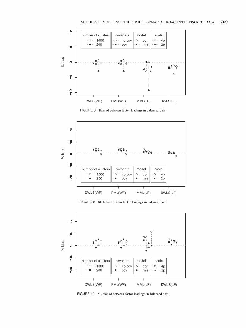
Bias of Factor Loadings. Figure 7 shows the rela-tive bias of the factor loadings at the within-level fordifferent estimation methods. In general, the bias is verylow across all conditions and only slightly higher in condi-tions with a misspecification and the MML estimationmethod. Figure 8 shows the relative bias of the between-level factor loadings for different estimation methods. Allmethods show increased bias at the between-level, espe-cially in conditions with a misspecification when the MMLestimation method was used. For this specific condition, therelative bias equals 7.12% for two point scales and 11.86%for four point scales.
Bias Standard Errors of Factor Loadings. Figures9 and 10 show the relative bias of the standard errors asso-ciated with the factor loadings at the within- and thebetween-level, respectively. Figure 9 shows small biasacross all conditions with the MML estimation method andthe estimation methods in the WF approach. The bias of the
standard errors at the between-level (see Figure 10) is smallacross all estimation methods, except for the MML estima-tion method where the relative bias is unexpectedly high.
Unbalanced Data
Bias of Factor Loadings. The relative bias of thefactor loadings with unbalanced data across all conditions atboth the within-level and the between-level generally showthe same picture as those with balanced data. Once again thebias in the MML estimation method is somewhat higher inconditions with a misspecification at the within-level andespecially high in conditions with a misspecification at thebetween-level. The corresponding figures are shown in thesupplementary materials.
Bias Standard Errors of Factor Loadings. Therelative bias of the standard errors associated with thefactor loadings at the within-level is shown in Figure 11.The bias is reasonable in the MML estimation method andthe WF approaches. Only the DWLS estimation method inthe LF approach shows a slightly deviant pattern in manyconditions. Figure 12 shows the relative bias of the stan-dard errors associated with the factor loadings at thebetween-level. The WF estimation methods show higherrelative bias across all conditions (i.e., about 10%). TheDWLS estimation method in the LF approach shows lowerbias than the other estimation methods and the MML esti-mation method shows more variation in the relative biasacross all conditions.
Bias Associated with Regression Coefficients ofthe Covariate
Overall, the relative bias in both the parameter estimatesand the associated standard errors related to the regressioncoefficients of the covariate is very low across all
−10
−50
510
% b
ias
−10
−50
510
−10
−50
510
−10
−50
510
−10
−50
510
−10
−50
510
−10
−50
510
−10
−50
510
−10
−50
510
−10
−50
510
−10
−50
510
−10
−50
510
−10
−50
510
−10
−50
510
−10
−50
510
−10
−50
510
DWLS(WF) PML(WF) MML(LF) DWLS(LF)
number of clusters
1000200
covariate
no covcov
model
cormis
scale
4p2p
FIGURE 7 Bias of within factor loadings in balanced data.
2 All R scripts (e.g., data generation scripts and scripts to analyze thedata) are available at the Open Science Foundation (OSF), following thelink https://osf.io/fa2gp/.
708 BARENDSE AND ROSSEEL
−20
−10
010
% b
ias
−20
−10
010
−20
−10
010
−20
−10
010
−20
−10
010
−20
−10
010
−20
−10
010
−20
−10
010
−20
−10
010
−20
−10
010
−20
−10
010
−20
−10
010
−20
−10
010
−20
−10
010
−20
−10
010
−20
−10
010
20
DWLS(WF) PML(WF) MML(LF) DWLS(LF)
number of clusters
1000200
covariate
no covcov
model
cormis
scale
4p2p
FIGURE 9 SE bias of within factor loadings in balanced data.
−20
−10
010
20
% b
ias
−20
−10
010
20−2
0−1
00
1020
−20
−10
010
20−2
0−1
00
1020
−20
−10
010
20−2
0−1
00
1020
−20
−10
010
20−2
0−1
00
1020
−20
−10
010
20−2
0−1
00
1020
−20
−10
010
20−2
0−1
00
1020
−20
−10
010
20−2
0−1
00
1020
−20
−10
010
20
DWLS(WF) PML(WF) MML(LF) DWLS(LF)
number of clusters
1000200
covariate
no covcov
model
cormis
scale
4p2p
FIGURE 10 SE bias of between factor loadings in balanced data.
−10
−50
510
% b
ias
−10
−50
510
−10
−50
510
−10
−50
510
−10
−50
510
−10
−50
510
−10
−50
510
−10
−50
510
−10
−50
510
−10
−50
510
−10
−50
510
−10
−50
510
−10
−50
510
−10
−50
510
−10
−50
510
−10
−50
510
DWLS(WF) PML(WF) MML(LF) DWLS(LF)
number of clusters
1000200
covariate
no covcov
model
cormis
scale
4p2p
FIGURE 8 Bias of between factor loadings in balanced data.
MULTILEVEL MODELING IN THE ‘WIDE FORMAT’ APPROACH WITH DISCRETE DATA 709

conditions and all estimation methods. The correspondingfigures are shown in the supplementary materials.
Summary of Results
With all estimation methods, the bias of the regressioncoefficients associatedwith the covariate and the correspondingstandard error at the within- and the between-level is largelyunbiased across all conditions. The bias of the factor loadingsand the associated standard errors show more variation acrossestimation methods and/or conditions. Overall, the bias of boththe factor loadings and the standard errors across all conditionsis higher at the between-level than at the within-level. The WFestimation methods are largely unbiased across conditions andmore relative bias of the standard errors at the between-level arenoticeablewith unbalanced data.TheDWLS estimationmethodin the LF approach shows a deviant pattern compared to allother estimation methods in many conditions. In general, the
MML estimationmethod in the LF approach exhibits more biasthan all other estimation methods. Perhaps most prominentlythe high bias in both the factor loadings and their associatedstandard errors in conditions with a misspecification.
In describing the parameter estimates, we did not men-tion the thresholds as these parameters are often not oftheoretical interest. For all conditions, the bias in thethresholds was very low for all estimation methods. Thefigures are shown in the supplementary materials.
ILLUSTRATION
Data
The WF approach to estimate multilevel data is illustratedwith data from the dependency scale of a Dutch translationof the Student-Teacher Relationship Scale (STRS; Koomen
−20
−10
010
20
% b
ias
−20
−10
010
20−2
0−1
00
1020
−20
−10
010
20−2
0−1
00
1020
−20
−10
010
20−2
0−1
00
1020
−20
−10
010
20−2
0−1
00
1020
−20
−10
010
20−2
0−1
00
1020
−20
−10
010
20−2
0−1
00
1020
−20
−10
010
20−2
0−1
00
1020
−20
−10
010
20
DWLS(WF) PML(WF) MML(LF) DWLS(LF)
number of clusters1000200
covariatenoyes
modelcorrectmis
scale4−point2−point
FIGURE 12 SE bias of between factor loadings in unbalanced data.
−20
−10
010
20
% b
ias
−20
−10
010
20−2
0−1
00
1020
−20
−10
010
20−2
0−1
00
1020
−20
−10
010
20−2
0−1
00
1020
−20
−10
010
20−2
0−1
00
1020
−20
−10
010
20−2
0−1
00
1020
−20
−10
010
20−2
0−1
00
1020
−20
−10
010
20−2
0−1
00
1020
−20
−10
010
20
DWLS(WF) PML(WF) MML(LF) DWLS(LF)
number of clusters1000200
covariatenoyes
modelcorrectmis
scale4−point2−point
FIGURE 11 SE bias of within factor loadings in unbalanced data.
710 BARENDSE AND ROSSEEL

et al., 2007). As the dataset contains small clusters sizes,the WF approach is very suitable. Through this example,we will show how the WF can be used to estimate multi-level models with different estimation methods. In thedataset of Koomen et al. (2007) primary school teachersfilled in six questions regarding overly dependent andclingy child behavior for only a few children (mean = 2.3)from their class, aged 3 to 12:
1. This child fixes his/her attention on me the whole daylong.
2. This child reacts strongly to separation from me.3. This child is overly dependent on me.4. This child asks for my help when he/she really does
not need help.5. This child expresses hurt or jealousy when I spend
time with other children.6. This child needs to be continually confirmed by me.
A multilevel one factor is specified using the six depen-dency items (see Figure 6 for a one factor model with 4items). Responses were given on a 5-point scale rangingfrom 1 (‘definitely does not apply’) to 5 (‘definitely doesapply’). For simplicity, we only selected classes whereteachers rated at most three children. This resulted in datafrom 1047 students (497 boys and 550 girls) that weregathered from 559 primary school teachers (144 men and415 woman) with an average cluster size of 1.873. Ina preliminary analysis a one factor model is fitted, treatingthe data as continuous, using ML with robust standarderrors and fit statistics. Note that with continuous data, theresults as well as the fit statistics of the WF approach areidentical to the results of the LF approach. This multilevelmodel fits the data well (χ2 (18) = 29.990, p = .038,RMSEA = 0.025, CFI = 0.992, SRMR (within-level)= 0.030, SRMR (between-level) = 0.073).
Statistical Analysis
Data were first reordered in the WF approach such that allthe children in a class are row-wise displayed. As not allclusters have an equal number of children, clusters withless than three children have missing values (i.e., designmissingness see Paragraph 1.3). We will use the sameestimation methods as the ones used in the simulationstudy (i.e., PML and DWLS in the WF approach andMML and DWLS in the LF approach) and mainly focuson the parameter estimates and the associated standarderrors. Similar to the simulation study, all WF approacheswere estimated with lavaan (Rosseel, 2012) and all LFapproaches were estimated with Mplus (Muthén &Muthén, 2010). The gender of the student (i.e., sk) andthe gender of the primary school teacher (i.e., sl) are thebinary covariates in the analysis.
We will fit the following multilevel models with theSTRS data in the WF approach:
● Model 0: Unstructured model without covariates● Model 1: CFA without covariates● Model 2: CFA without covariates with measurementinvariance restrictions
● Model 3: Unstructured model with binary covariates● Model 4: CFA with binary covariates● Model 5: CFA with binary covariates with measure-ment invariance restrictions
● Model 6: Unstructured model with continuouscovariates
● Model 7: CFA with continuous covariates● Model 8: CFA with continuous covariates with mea-surement invariance restrictions
All models are fitted according to the proposed stepsin section “WF Approach with Discrete Data3.” Wesubsequently fit three models without covariates(Model 0 - Model 2), three models with the covariatestreated as categorical (Model 3 - Model 5), and threemodels with covariates treated as continuous (Model 6 -Model 8). Note that estimation methods in the LFapproach do not need unstructured models (Model 0and Model 3).
In models without restrictions (Model 1, Model 4, andModel 7), the factor loadings at the within-level can bedifferent from the factor loadings at the between-level andthe residuals at the between-level (i.e., random intercept var-iances leftover) are freely estimated. These kind of multilevelmodels have a complicated interpretation as the within-levelfactor loadings should then be interpreted as a summary of allpossible cluster factor loadings. Nevertheless, the model with-out restrictions can serve as a baseline model for models withrestrictions across clusters. Models with measurement invar-iance restrictions (Model 2, Model 5, and Model 8) ensurethat factors have the same interpretation across all clusters,and restrictions on the residuals at the between-level ensurethat the clusters have the same intercepts and that no othervariables than the specified latent variables are affecting thebetween-level responses (see Mehta & Neale, 2005; Muthén,1990; Rabe-Hesketh et al., 2004a).
It is important to note that the MML estimation methodcannot estimate Model 0 or CFA models without measure-ment invariance restrictions, as the number of latent vari-ables in all other models exceeds the number of dimensionsthe MML estimation method can handle. This has to do
3The syntax can be found at the OSF. The syntax used to fit the STRSdata is quite similar to the syntax printed in Appendix D (see AppendixB for adding covariates).
MULTILEVEL MODELING IN THE ‘WIDE FORMAT’ APPROACH WITH DISCRETE DATA 711

with the estimation of the errors on the between-level, thatare modeled as additional latent variables.
Results
To briefly illustrate the use of fit statistics in the WF approach,Table 1 contains the intra-class coefficients (ICC) according tothe DWLS and PML estimation methods in the WF approachand the DWLS estimationmethod in the LF approach. The ICCvalues are almost equivalent across estimation methods.Forcing the MML to calculate the ICC will lead to too manylatent variables which is computationally too intensive. Table 2shows the χ2 values and the degrees of freedom of the modelsof interest and the unstructured models for the STRS data usingthe DWLS estimation method with the scaled and shifted teststatistic (Asparouhov & Muthén, 2010). In the WF approach,the model of interest and the unrestricted model are necessaryto obtain the multilevel test statistic. The last two columnsindicate the chi-square test statistics and the associated degreesof freedom for the various multilevel models obtained viaa scaled chi-square difference test (Satorra, 2000). The resultsindicate that the general model with or without covariates fitsthe data well, while models with invariance restrictions do notfit the data. To give a general idea of the estimation time of theused estimation methods, we saved the estimation time ofa model without covariates and errors on the between level;DWLS in the WF approach: 0.11 minutes, PML in the WFapproach: 3.24 minutes, MML in the long format approach:4:25 minutes, and DWLS in the LF approach: 1:53 minutes.
Column 2 to 5 of Table 3 contains the parameter esti-mates and the standard errors of a model without measure-ment invariance restrictions across levels for differentestimation methods with a discrete covariate. Only thetheta parameterization ensures that the WF approach iscomparable to the LF approaches. As the DWLS estimationmethod in the LF approach cannot include the covariate asa discrete covariate, Column 6 to 11 contain the parameterestimates and the standard errors of a model without mea-surement invariance restrictions across levels for differentestimation methods with a continuous covariate. Duringestimation we noticed that the DWLS in the WF approachhad problems constructing a weight matrix (i.e., W), whichis most likely due to treating the binary covariates as
continuous. The model shown in Table 3 contains toomany dimensions (i.e., six errors variances at the between-level and two latent variables) to estimate this model withthe MML estimation method in the LF approach.
The results of Table 3 indicate that the parameter estimatesof the PML estimation method and the DWLS estimationmethod in the WF approach are quite similar and only theparameter estimates for the DWLS estimation method in theLF approach are somewhat deviating. For all estimationmeth-ods, the error variances are not equal to zero, which indicatethat the intercepts of all classes are not equal to each other andthat other variables than the specified latent variables mayaffect the between-level responses.
Column 2 to 7 of Table 4 show the parameter estimatesand the standard errors of the STSR models with measure-ment invariance restrictions across levels. The model fitspoor in terms of the χ2 fit statistic, however, the calculationof the Correlation Root Mean Squared Residual (CRMR;Bentler, 1985; Maydeu-Olivares, 2017; Ogasawara, 2001),that is less dependent on the sample size, showed reason-able fit values (e.g., 0.0148, z = 1.425, p > .05 for Model 2).The measurement invariance restrictions facilitate the inter-pretation of the effect of the covariates. As boys werescored 0 and girls 1, the unstandardized effect of depen-dency on the gender of the child equals 0.106 in, forexample, the WF DWLS estimation method witha discrete covariate. This means that teachers experiencemore dependency with girls than with boys. The unstandar-dized direct effect in the WF DWLS of dependency on thegender of the teacher is −0.098 indicating that male tea-chers experience more dependency than female teachers.Overall, the parameter estimates of the multilevel MML arequite similar to the ones obtained by the WF approach. Theeffect of the covariate is also about equal in terms of ratios.The parameter estimates of the LF DWLS are again some-what deviating. The last six columns of Table 4 show theparameter estimates and the standard errors of the modelswith and without measurement invariance restrictions withcontinuous covariates in the WF approach.
TABLE 1ICC for Different Estimation Methods
DWLS(LF) DWLS(WF) PML(WF)
Item 1 0.463 0.460 0.453Item 2 0.362 0.409 0.379Item 3 0.145 0.151 0.137Item 4 0.274 0.276 0.283Item 5 0.421 0.417 0.412Item 6 0.203 0.207 0.204
TABLE 2χ2 Test Statistics for the DWLS Estimation Method in the WF
H1 H0 model fit
df χ2 df χ2 df χ2
Models without covariatesModel 0 & Model 1: 164 152.111 182 166.752 18 8.010Model 0 & Model 2: 164 152.111 193 310.396 29 112.336*Models with binary covariatesModel 3 & Model 4: 226 212.385 254 238.925 28 20.783Model 3 & Model 5: 226 212.385 265 389.558 39 135.324*Models with covariatesModel 6 & Model 7: 234 168.540 262 192.628 28 19.000Model 6 & Model 8: 234 168.540 273 342.596 39 133.402*
Note: * = p <0.05
712 BARENDSE AND ROSSEEL

Conclusion
The STRS data shows that the WF approach can be used indatasets with a relatively small number of units in each cluster.Using the stepwise approach from section “Multilevel SEM inthe WF Approach” and section “WF Approach with DiscreteData”, various CFA models, including models with covariatesand measurement bias restrictions, can be fitted to the STRSdata. The DWLS in both the LF- andWF approch and the PMLestimation method can estimate all suggested models. Due tothe increasing dimensionality, the MML estimation methodcannot fit models with error variances on the between-level(see Table 3). We hesitate to interpret the results of the theDWLS estimation method in the LF approach, as it showsa different pattern of parameter estimates compared to allother estimation methods.
Discussion
In this article, we united the fragmented literature on theWF approach into a general framework for random
intercept SEM multilevel models for a small number ofobservations in a cluster that can handle unbalanced data,missing data, and covariates at both the within- and thebetween-level. In addition, we also extent the WF approachfor discrete data and provide an illustration. With smallcluster sizes, the least squares estimation methods and thePML estimation method are very useful to fit all multilevelmodels in the WF approach. Only the MML estimationmethod is harder to use in the WF approach as it is com-putationally very intensive and only of practical use in theestimation of multilevel regression or path models. Tomake the WF approach applicable, we used the OpenScience Framework to provide the readers with theR script of the empirical example, and the R scripts andartificial data that corresponds to the models presented inthe appendix.
In general, modeling multilevel data in the WF approachhas several advantages over modeling multilevel data in theLF approach. First, the WF approach is computationallyvery efficient compared to the MML estimation method in
TABLE 3Parameter Estimates of Model 4 and Model 7
binary covariate continuous covariate
DWLS(WF) PML(WF) DWLS(WF) PML(WF) DWLS(LF)
θ SE Var SE Var SE Var SE :52 � 1 SE
λw1;1 1.000 - 1.000 - 1.000 - 1.000 - 1.000 -
λw1;2 2.475 0.446 2.352 0.426 2.477 0.446 2.361 0.434 2.029 0.319
λw1;3 2.058 0.354 1.947 0.364 2.008 0.340 1.951 0.367 1.589 0.242
λw1;4 1.428 0.247 1.445 0.257 1.392 0.238 1.445 0.258 1.166 0.177
λw1;5 1.889 0.307 1.864 0.322 1.874 0.302 1.862 0.325 1.574 0.222
λw1;6 3.097 0.592 3.069 0.679 3.161 0.618 3.053 0.681 2.186 0.333
VarðηwÞ 0.217 0.064 0.221 0.069 0.222 0.065 0.223 0.070 0.325 0.077VarðskÞ - - - - 0.249 0.003 0.250 0.001 - -IntðskÞ - - - - 0.535 0.021 0.521 0.012 - -ηw on sk 0.073 0.026 0.070 0.026 0.108 0.054 0.112 0.042 0.141 0.050
λb1;1 1.000 - 1.000 - 1.000 - 1.000 - 1.000 -
λb1;2 1.259 0.207 1.227 0.222 1.264 0.209 1.229 0.227 1.281 0.230
λb1;3 0.517 0.115 0.503 0.117 0.519 0.114 0.503 0.117 0.544 0.119
λb1;4 0.835 0.164 0.833 0.164 0.840 0.164 0.833 0.164 0.892 0.183
λb1;5 0.934 0.126 0.965 0.137 0.936 0.127 0.965 0.142 1.034 0.169
λb1;6 0.608 0.129 0.610 0.153 0.613 0.133 0.609 0.156 0.652 0.139
VarðηbÞ 0.749 0.172 0.689 0.156 0.761 0.173 0.701 0.160 0.658 0.170
ηb on sl −0.174 0.078 −0.163 0.077 −0.287 0.131 −0.271 0.128 −0.248 0.124
VarðslbÞ - - - - 0.191 0.009 0.195 0.007 - -IntðslÞ - - - - 0.742 0.007 0.734 0.015 - -
Θb1;1
0.261 0.143 0.304 0.132 0.267 0.143 0.304 0.133 0.483 0.138
Θb2;2
0.395 0.206 0.299 0.186 0.404 0.210 0.306 0.188 0.244 0.157
Θb3;3
0.138 0.114 0.115 0.097 0.131 0.111 0.116 0.098 0.113 0.095
Θb4;4
0.011 0.111 0.083 0.116 0.001 0.109 0.083 0.116 0.021 0.107
Θb5;5
0.604 0.188 0.587 0.182 0.603 0.187 0.585 0.180 0.611 0.138
Θb6;6
0.530 0.233 0.534 0.239 0.557 0.248 0.527 0.237 0.370 0.129
Note: (1) Thresholds are not shown here; (2) For identification purposes the first factor loading on the between-level and the within-level are fixed to one.
MULTILEVEL MODELING IN THE ‘WIDE FORMAT’ APPROACH WITH DISCRETE DATA 713

the LF approach opening up the possibility to analyzemodels with many latent variables. The illustration showedthat a simple one factor model with errors on the between-level contains already too many latent variables to estimatewith the MML estimation method in the LF approach.Estimating this model in the WF approach with PML andDWLS causes no problems. This offers new possibilities toestimate factor models with errors on the between-level.Second, the WF approach does not need as many restric-tions as the LF approach. Where the LF approach implicitlyforces equality constraints on, for example, the factor load-ings and the thresholds across clusters, the WF approachcan test all these restrictions. Third, there is no special SEMsoftware needed to perform multilevel analysis with dis-crete data, as single level software is capable of performingthe multilevel analysis. Despite the potential advantages,there are of course a number of limitations. First, largercluster sizes and/or more variables require a larger numberof clusters. Second, highly unbalanced data are problematicin the WF approach. If, for example, all clusters contain nomore than five units, except for one cluster with twentyunits, we would advice to randomly sample five units fromthis cluster to deal with this highly unbalanced data in theWF approach. Third, it is tedious to specify a multilevelmodel in the WF approach using current SEM software. Asthe maximum number of units increase, the size of themodel syntax increases too. In the future, we plan todevelop scripts that will automatically generate the modelsyntax.
The simulation study showed that the estimation meth-ods in the WF approach are capable to estimate multilevel
models under the simulated conditions. The parameter esti-mates of the estimation methods in this simulation studywith the WF approach are largely unbiased and not somuch influenced by the balancedness of the data, the num-ber of clusters, and model misspecification. It is noticeablethat the bias of the parameter estimates and the standarderrors at the between-level are larger than the bias at thewithin-level. Of course, the between-level contains lessunits than the within-level, which influences the bias ofthe parameter estimates and the standard errors. TheDWLS and the PML estimation method in the WFapproach show very similar results, which can be explainedby the fact that they both rely on bivariate information. TheMML estimation method in the LF approach shows com-parable results to the estimation methods in the WFapproach, except in conditions with a misspecification,where the bias in the parameter estimates is alarminglyhigh. The high bias of the standard errors at the between-level with four response scales in the MML estimationmethod, was also surprising. The DWLS estimation methodin the LF approach is hindered by some convergence pro-blems and shows a different pattern of results compared toall other estimation methods. As it is impossible to considerall plausible scenarios in a single simulation study, general-ization beyond the range of the conditions studied shouldbe undertaken with caution.
The illustrative dataset on the student-teacher relation-ship shows that the WF approach is capable of estimatingdifferent multilevel models in real data. If the MML esti-mation is feasible (as in Table 4), the results of the WFapproach are very similar to the results of the MML
TABLE 4Parameter Estimates of Model 5 and Model 8
binary covariate continuous covariate
DWLS(WF) PML(WF) MML(LF) DWLS(WF)PML(WF)
DSMV(LF)
θ SE θ SE θ SE θ SE θ SE θ SE
λ1;1 1.000 - 1.000 - 1.000 - 1.000 - 1.000 - 1.000 -λ1;2 1.611 0.167 1.697 0.204 1.845 0.186 1.613 0.168 1.697 0.209 1.881 0.256λ1;3 0.994 0.103 0.993 0.126 1.174 0.117 0.989 0.102 0.993 0.127 1.206 0.151λ1;4 1.115 0.126 1.161 0.142 1.246 0.129 1.109 0.125 1.161 0.140 1.109 0.151λ1;5 1.138 0.101 1.224 0.121 1.300 0.120 1.136 0.100 1.224 0.124 1.469 0.173λ1;6 1.081 0.105 1.100 0.139 1.318 0.130 1.080 0.105 1.101 0.141 1.554 0.175VarðηwÞ 0.409 0.070 0.374 0.062 0.324 0.052 0.415 0.070 0.377 0.064 0.440 0.086VarðskÞ - - - - - - 0.249 0.003 0.250 0.001 - -IntðskÞ - - - - - - 0.535 0.021 0.521 0.012 - -ηw on sk 0.106 0.037 0.095 0.035 0.143 0.050 0.157 0.082 0.152 0.056 0.164 0.057VarðηbÞ 0.346 0.072 0.289 0.068 0.266 0.053 0.351 0.073 0.293 0.070 0.267 0.065
ηb on sl −0.098 0.052 −0.089 0.049 −0.119 0.072 −0.162 0.088 −0.148 0.081 −0.127 0.078
VarðslbÞ - - - - - - 0.191 0.009 0.195 0.007 - -IntðslÞ - - - - - - 0.742 0.007 0.734 0.015 - -
Note:(1) Thresholds are not shown here; (2) For identification purposes the first factor loading on the between-level and the within-level are fixed to one.
714 BARENDSE AND ROSSEEL

estimation method in the LF approach. The results of theDWLS in the LF approach are typically somewhat deviant.Although we did not encounter difficulties with empty cellsin our example, empty cells caused by within-cluster miss-ingness or design missingness can be problematic in theWF approach. Potential solutions for datasets with emptycells are discussed by Agresti and Yang (1987).
In the illustration, we briefly showed how to calculatethe χ2 goodness-of-fit statistic in the WF approach. As thefit in a multilevel model expresses the combined (mis)fit atboth the within- and the between-level, more attentionshould be given to this topic. The within-level has generallymore influence on the overall fit than the between-level, asthe number of units at the within-level is higher than thenumber of units at the between-level. Ryu and West (2009)and Boulton (2011) proposed level specific fit measures formultilevel SEM.
In this study, we only considered models with a randomintercept. Multilevel models can be extended by addingrandom slopes, where the impact of covariates is allowedto vary across clusters. The estimation of random slopesrequires case-wise estimation. With discrete data in the LF,only the MML estimation method can estimate models witha random slope. In the WF approach, the PML estimationmethod seems best suited to estimate models includinga random slope in for example generalized linear mixedmodels (see Bellio & Varin, 2005; Cho & Rabe-Hesketh,2011; Tibaldi et al., 2007). Compared to the MML in theLF approach, the PML estimation method in the WFapproach can in theory estimate many random slopes andother latent variables. The WLS estimation method in theWF approach uses a two-step estimation procedure and cantherefore not estimate models with random slopes.
The PML estimation method seems a promising, perhapsunderused, estimation method that was initially developed fordiscrete data (see Jöreskog & Moustaki, 2001). So far, exo-genous covariates in the PML estimation method areregressed out first and further calculations are done on theresidual correlations. However, in the WF approach the cov-ariates are considered as stochastic variables, where the PMLestimation method has to deal with pairs of variables that arepotentially a mixture of discrete and continuous variables andcombinations thereof. This is the first study that deals witha mixture of discrete and continuous variables in estimatingSEM with the PML estimation method. As mentioned above,the PML estimation method is also capable of estimatingrandom slopes. In addition, with very unequal cluster sizes,the PML estimation method could be extended by usingweights (e.g., Joe & Lee, 2009; Renard, 2002).
In future research, the WF approach can easily beextended to more than two levels or used to estimate multi-group multilevel models or multilevel longitudinal models,where the mean structure is also of importance. Additionally,
the possibilities of the PML estimation method with case-wise estimation can be explored to estimate models withrandom slopes and/or models in the WF approach wherethe number of columns (variables � observations) is largerthan the number of rows (number of clusters).
ACKNOWLEDGEMENTS
The authors thank Helma Koomen of the University ofAmsterdam for making her data available for secondary analy-sis. We are also thankful to Karin Schermelleh-Engel and WenWei Loh for helpful comments on an earlier draft of this article.
FUNDING
This publication is supported by Special Research Fund(BOF) open competition grant from Ghent University.
ORCID
M.T. Barendse http://orcid.org/0000-0002-1632-0303Y. Rosseel http://orcid.org/0000-0002-4129-4477
REFERENCES
Agresti, A., & Yang, M.-C. (1987). An empirical investigation of someeffects of sparseness in contingency tables. Computational Statistics &Data Analysis, 5, 9–21. doi:10.1016/0167-9473(87)90003-X
Arbuckle, J. L. (1996). Full information estimation in the presence ofincomplete data. In G. In Marcoulides & R. Schumacker (Eds.),Advanced structural equation modeling: Issues and techniques (pp.243–277). Mahwah, NJ: Erlbaum.
Asparouhov, T., & Muthén, B. (2007, August). Computationally efficientestimation of multilevel high-dimensional latent variable models. Inproceedings of the 2007 JSM meeting in Salt Lake City, Utah, Sectionon Statistics in Epidemiology (pp. 2531–2535).
Asparouhov, T., & Muthén, B. (2010). Simple second order chi-squarecorrection. Mplus technical appendix.
Bauer, D. J. (2003). Estimating multilevel linear models as structuralequation models. Journal of Educational and Behavioral Statistics,28, 135–167. doi:10.3102/10769986028002135
Beauducel, A., & Herzberg, P. Y. (2006). On the performance of maximumlikelihood versus means and variance adjusted weighted least squaresestimation in cfa. Structural Equation Modeling, 13, 186–203.doi:10.1207/s15328007sem1302_2
Bellio, R., & Varin, C. (2005). A pairwise likelihood approach to general-ized linear models with crossed random effects. Statistical Modelling, 5,217–227. doi:10.1191/1471082X05st095oa
Bentler, P. M., & Dijkstra, T. (1985). Efficient estimation via linearizationin structural models. In PR Krishnaiah (Ed.), Multivariate Analysis (Vol.6, pp.9–42)..
Bock, R. D., & Aitkin, M. (1981). Marginal maximum likelihood estima-tion of item parameters: Application of an em algorithm.Psychometrika, 46, 443–459. doi:10.1007/BF02293801
MULTILEVEL MODELING IN THE ‘WIDE FORMAT’ APPROACH WITH DISCRETE DATA 715

Bollen, K. A. (1989). Structural equations with latent variables.New York, NY: John Wiley & Sons.
Boulton, A. J. (2011). Fit index sensitivity in multilevel structural equationmodeling (PhD thesis). University of Kansas.
Browne, M. W. (1984). Asymptotically distribution–Free methods for theanalysis of covariance structures. British Journal of Mathematical andStatistical Psychology, 37, 62–83. doi:10.1111/bmsp.1984.37.issue-1
Browne, M. W. (1995). Covariance structures. In Topics in applied multi-variate analysis (pages 72–141). ID M. Hawkins. Cambridge, UK:Cambridge University Press.
Bryk, A. S., & Raudenbush, S. W. (1987). Application of hierarchicallinear models to assessing change. Psychological Bulletin, 101,147–158. doi:10.1037/0033-2909.101.1.147
Cai, L. (2010). A two-tier full-information item factor analysis model withapplications. Psychometrika, 75, 581–612. doi:10.1007/s11336-010-9178-0
Cho, S.-J., & Rabe-Hesketh, S. (2011). Alternating imputation posteriorestimation of models with crossed random effects. ComputationalStatistics & Data Analysis, 55, 12–25. doi:10.1016/j.csda.2010.04.015
Chou, C.-P., Bentler, P. M., & Pentz, M. A. (1998). Comparisons of twostatistical approaches to study growth curves: The multilevel model and thelatent curve analysis. Structural Equation Modeling, 5, 247–266.doi:10.1080/10705519809540104
Croon, M. A., & van Veldhoven, M. J. (2007). Predicting group-leveloutcome variables from variables measured at the individual level:A latent variable multilevel model. Psychological Methods, 12, 45.doi:10.1037/1082-989X.12.1.45
Curran, P. J. (2003). Have multilevel models been structural equationmodels all along? Multivariate Behavioral Research, 38, 529–569.doi:10.1207/s15327906mbr3804_5
Depaoli, S., & Clifton, J. P. (2015). A bayesian approach to multilevelstructural equation modeling with continuous and dichotomousoutcomes. Structural Equation Modeling, 22, 327–351. doi:10.1080/10705511.2014.937849
Dyer, N. G., Hanges, P. J., & Hall, R. J. (2005). Applying multilevelconfirmatory factor analysis techniques to the study of leadership.The Leadership Quarterly, 16, 149–167. doi:10.1016/j.leaqua.2004.09.009
Flora, D. B., & Curran, P. J. (2004). An empirical evaluation of alternativemethods of estimation for confirmatory factor analysis with ordinaldata. Psychological Methods, 9, 466–491. doi:10.1037/1082-989X.9.4.466
Fox, J.-P. (2010). Bayesian item response modeling: Theory and applica-tions. New York, NY: Springer Science & Business Media.
Goldstein, H., & McDonald, R. P. (1988). A general model for the analysisof multilevel data. Psychometrika, 53, 455–467. doi:10.1007/BF02294400
Guo, B., Perron, B. E., & Gillespie, D. F. (2008). A systematic review ofstructural equation modelling in social work research. British Journal ofSocial Work, 39, 1556–1574. doi:10.1093/bjsw/bcn101
Hedeker, D., & Gibbons, R. D. (1994). A random-effects ordinal regres-sion model for multilevel analysis. Biometrics, 933–944. doi:10.2307/2533433
Holtmann, J., Koch, T., Lochner, K., & Eid, M. (2016). A comparisonof ml, wlsmv, and bayesian methods for multilevel structural equa-tion models in small samples: A simulation study. MultivariateBehavioral Research, 51, 661–680. doi:10.1080/00273171.2016.1208074
Hox, J. J., Moerbeek, M., & Van de Schoot, R. (2017). Multilevel analysis:Techniques and applications. New York, NY: Routledge.
Joe, H., & Lee, Y. (2009). On weighting of bivariate margins in pairwiselikelihood. Journal of Multivariate Analysis, 100, 670–685.doi:10.1016/j.jmva.2008.07.004
Jöreskog, K. G. (1981). Analysis of covariance structures. ScandinavianJournal of Statistics, 8, 65–92.
Jöreskog, K. G., & Moustaki, I. (2001). Factor analysis of ordinal vari-ables: A comparison of three approaches. Multivariate BehavioralResearch, 36, 347–387. doi:10.1207/S15327906347-387
Katsikatsou, M., & Moustaki, I. (2016). Pairwise likelihood ratio tests andmodel selection criteria for structural equation models with ordinalvariables. Psychometrika, 81, 1046–1068. doi:10.1007/s11336-016-9523-z
Katsikatsou, M., & Moustaki, I. (2017). Pairwise likelihood estimation forconfirmatory factor analysis models with ordinal variables and data thatare missing at random. Submitted to Journal of Royal Statistical SocietySeries C.
Katsikatsou, M., Moustaki, I., Yang-Wallentin, F., & Jöreskog, K. G.(2012). Pairwise likelihood estimation for factor analysis models withordinal data. Computational Statistics & Data Analysis, 56, 4243–4258.doi:10.1016/j.csda.2012.04.010
Kim, E. S., Yoon, M., Wen, Y., Luo, W., & Kwok, O.-M. (2015). Within-level group factorial invariance with multilevel data: Multilevel factormixture and multilevel mimic models. Structural Equation Modeling,22, 603–616. doi:10.1080/10705511.2014.938217
Koomen, H., Verschueren, K., & Pianta, R. C. (2007). Leerling leerkrachtrelatie vragenlijst- handleiding g. [Student–Teacher Relationship Scale:Manual]. Houten: Bohn Stafleu van Loghum.
Koomen, H. M., Verschueren, K., van Schooten, E., Jak, S., &Pianta, R. C. (2012). Validating the student-teacher relationship scale:Testing factor structure and measurement invariance across child genderand age in a dutch sample. Journal of School Psychology, 50, 215–234.doi:10.1016/j.jsp.2011.09.001
Lee, J. (2009). Universals and specifics of math self-concept, mathself-efficacy, and math anxiety across 41 pisa 2003 participatingcountries. Learning and Individual Differences, 19, 355–365.doi:10.1016/j.lindif.2008.10.009
Li, H., Fortner, C. K., & Lei, X. (2015). Relationships between the use oftest results and us students’ academic performance. School Effectivenessand School Improvement, 26, 258–278. doi:10.1080/09243453.2014.898662
Lindsay, B. G. (1988). Composite likelihood methods. ContemporaryMathematics, 80, 221–239.
Lüdtke, O., Marsh, H. W., Robitzsch, A., Trautwein, U., Asparouhov, T.,& Muthén, B. (2008). The multilevel latent covariate model: A new,more reliable approach to group-level effects in contextual studies.Psychological Methods, 13, 203. doi:10.1037/a0012869
MacCallum, R. C., & Austin, J. T. (2000). Applications of structuralequation modeling in psychological research. Annual Review ofPsychology, 51, 201–226. doi:10.1146/annurev.psych.51.1.201
MacCallum, R. C., Kim, C., Malarkey, W. B., & Kiecolt-Glaser, J. K.(1997). Studying multivariate change using multilevel models and latentcurve models. Multivariate Behavioral Research, 32, 215–253.doi:10.1207/s15327906mbr3203_1
Maydeu-Olivares, A. (2017). Assessing the size of model misfit in struc-tural equation models. Psychometrika, 82, 533–558. doi:10.1007/s11336-016-9552-7
McArdle, J. J., & Epstein, D. (1987). Latent growth curves within devel-opmental structural equation models. Child Development, pages 110–133. doi:10.2307/1130295
McDonald, R. P. (1993). A general model for two-level data withresponses missing at random. Psychometrika, 58, 575–585.doi:10.1007/BF02294828
McDonald, R. P., & Goldstein, H. (1989). Balanced versus unbalanceddesigns for linear structural relations in two-level data. British Journalof Mathematical and Statistical Psychology, 42, 215–232. doi:10.1111/bmsp.1989.42.issue-2
Mehta, P. D., & Neale, M. C. (2005). People are variables too: Multilevelstructural equations modeling. Psychological Methods, 10, 259–283.doi:10.1037/1082-989X.10.3.259
Meredith, W., & Tisak, J. (1990). Latent curve analysis. Psychometrika,55, 107–122. doi:10.1007/BF02294746
716 BARENDSE AND ROSSEEL
Merz, E. L., & Roesch, S. C. (2011). Modeling trait and state variationusing multilevel factor analysis with panas daily diary data. Journal ofResearch in Personality, 45, 2–9. doi:10.1016/j.jrp.2010.11.003
Muthén, B., Du Toit, S. H., & Spisic, D. (1997). Robust inference usingweighted least squares and quadratic estimating equations in latentvariable modeling with categorical and continuous outcomes.Psychometrika, 75, 1–45.
Muthén, B. O. (1989). Latent variable modeling in heterogeneouspopulations. Psychometrika, 54, 557–585.
Muthén, B. O. (1990). Mean and covariance structure analysis of hier-archical data (Vol. 62, pp. 1–64). Los Angeles, LA: University ofCalifornia: Department of Statistics (UCLA Statistics Series).
Muthén, B. O., & Satorra, A. (1995). Technical aspects of Muthén’sliscomp approach to estimation of latent variable relations witha comprehensive measurement model. Psychometrika, 60, 489–503.
Muthén, L. K., & Muthén, B. O. (2010). Mplus: Statistical analysis withlatent variables: User’s guide. Los Angeles, CA: Muthén &Muthén.
Neale, M. C. (2000). Modeling longitudinal and multilevel data: Practicalissues, applied approaches and specific examples. In T. D. Little,K. U. Schnabel, & J. Baumert (Eds.), Individual fit, heterogeneity, andmissing data in multigroup sem (pp. 249–267). Hillsdale, NJ: Erlbaum.
NLSAH. (2005). National longitudinal study of adolescent health.Retrieved from http//:www.cpc.unc.edu/addhealth
Ogasawara, H. (2001). Standard errors of fit indices using residuals instructural equation modeling. Psychometrika, 66, 421–436. doi:10.1007/BF02294443
Olsson, U. (1979). Maximum likelihood estimation of the polychoriccorrelation coefficient. Psychometrika, 44, 443–460. doi:10.1007/BF02296207
Olsson, U., Drasgow, F., & Dorans, N. J. (1982). The polyserial correla-tion coefficient. Psychometrika, 47, 337–347. doi:10.1007/BF02294164
Rabe-Hesketh, S., Skrondal, A., & Pickles, A. (2004a). Generalized multi-level structural equation modeling. Psychometrika, 69, 167–190.doi:10.1007/BF02295939
Rabe-Hesketh, S., Skrondal, A., & Pickles, A. (2004b). Gllamm manual.uc berkeley division of biostatistics (working paper series 1160).University of California, Berkeley.
Renard, D. (2002). Topics in modeling multilevel and longitudinal data(Doctoral dissertation). Belgium.
Rosseel, Y. (2012). lavaan: An R package for structural equation modeling.Journal of Statistical Software, 48, 1–36. doi:10.18637/jss.v048.i02
Ryu, E., & West, S. G. (2009). Level-specific evaluation of model fit in multi-level structural equation modeling. Structural Equation Modeling, 16,583–601. doi:10.1080/10705510903203466
Satorra, A. (2000). Scaled and adjusted restricted tests in multi-sampleanalysis of moment structures. In Innovations in multivariate statisticalanalysis (pp. pages 233–247). Boston, MA: Springer.
Satorra, A., & Bentler, P. M. (1994). Corrections to test statistics andstandard errors in covariance structure analysis. In Clogg and Clogg(Ed.), Latent variables analysis: Applications for developmentalresearch (pp.399–419). Thousand Oaks, CA: Sage.
Schilling, S., & Bock, R. D. (2005). High-dimensional maximum marginallikelihood item factor analysis by adaptive quadrature. Psychometrika,70, 533–555.
Schmidt, W. H. (1969). Covariance structure analysis of the multivariaterandom effects model (PhD thesis). University of Chicago, Departmentof Education.
Snijders, T., & Bosker, R. J. (1999). Multilevel analysis: An introductionto basic and advanced multilevel modeling. London, UK: Sage.
Tibaldi, F. S., Verbeke, G., Molenberghs, G., Renard, D., Noortgate, W., &Boeck, P. (2007). Conditional mixed models with crossed randomeffects. British Journal of Mathematical and Statistical Psychology,60, 351–365. doi:10.1348/000711006X110562
Varin, C. (2008). On composite marginal likelihoods. Advances inStatistical Analysis, 92, 1–28. doi:10.1007/s10182-008-0060-7
Willett, J. B., & Sayer, A. G. (1994). Using covariance structure analysisto detect correlates and predictors of individual change over time.Psychological Bulletin, 116, 363. doi:10.1037/0033-2909.116.2.363
Wirth, R., & Edwards, M. C. (2007). Item factor analysis: Currentapproaches and future directions. Psychological Methods, 12, 58.doi:10.1037/1082-989X.12.1.58
Yang, Y. (2018). Structural equation modelling. In P. Brough (Ed.),Advanced research methods for applied psychology (pp. 258–270).New York, NY: Routledge.
Yang-Wallentin, F., Jöreskog, K. G., & Luo, H. (2010). Confirmatoryfactor analysis of ordinal variables with misspecified models.Structural Equation Modeling, 17, 392–423. doi:10.1080/10705511.2010.489003
MULTILEVEL MODELING IN THE ‘WIDE FORMAT’ APPROACH WITH DISCRETE DATA 717

APPENDIX
Appendix A: lavaan syntax for a multilevel one factor model with a covariate on both levels (i.e., w and z) in the WFapproach
# Syntax corresponding to Figure 2 with three observations in each cluster model <- ’
### Step 2: Model for the within level### Step 3: Equality constraints on the within level (labels e to h =### within factor loadings (λ), fvw1 to fvw3 = within factors (ηf w),### and rw1 to rw4 = residuals variances (Θ))# within structure via factor loadings and within factors variancesfw1 =∼ e*y1.1 + f*y2.1 + g*y3.1 + h*y4.1fw2 =∼ e*y1.2 + f*y2.2 + g*y3.2 + h*y4.2fw3 =∼ e*y1.3 + f*y2.3 + g*y3.3 + h*y4.3fw1 ∼∼ fvw*fw1fw2 ∼∼ fvw*fw2fw3 ∼∼ fvw*fw3
# uncorrelated fw1, fw2, fw3fw1 ∼∼ 0*fw2 + 0*fw3; fw2 ∼∼ 0*fw3
# within intercepts (fixed to zero)y1.1 + y2.1 + y3.1 + y4.1 ∼ 0*1y1.2 + y2.2 + y3.2 + y4.2 ∼ 0*1y1.3 + y2.3 + y3.3 + y4.3 ∼ 0*1
# common residual variancesy1.1 ∼∼ rw1*y1.1; y1.2 ∼∼ rw1*y1.2; y1.3 ∼∼ rw1*y1.3y2.1 ∼∼ rw2*y2.1; y2.2 ∼∼ rw2*y2.2; y2.3 ∼∼ rw2*y2.3y3.1 ∼∼ rw3*y3.1; y3.2 ∼∼ rw3*y3.2; y3.3 ∼∼ rw3*y3.3y4.1 ∼∼ rw4*y4.1; y4.2 ∼∼ rw4*y4.2; y4.3 ∼∼ rw4*y4.3
### Step 4: construct latent variables that represent random intercepts### of the variables y1,y2,y3, and y4 on the between levelby1 =∼ 1*y1.1 + 1*y1.2 + 1*y1.3by2 =∼ 1*y2.1 + 1*y2.2 + 1*y2.3by3 =∼ 1*y3.1 + 1*y3.2 + 1*y3.3by4 =∼ 1*y4.1 + 1*y4.2 + 1*y4.3
# between interceptsby1 + by2 + by3 + by4 ∼ 1
### Step 5: construct a model at the between level# between factorfb =∼ a*by1 + b*by2 + c*by3 + d*by4
# residual variances on the between-levelby1 ∼∼ by1; by2 ∼∼ by2; by3 ∼∼ by3; by4 ∼∼ by4
# between factor not correlated with the within factors fb ∼∼ 0*fw1 + 0*fw2 + 0*fw3’
# fitting the model with MLfit <- sem(model, data = wideData)summary(fit)
718 BARENDSE AND ROSSEEL

Appendix B: additional lavaan syntax to add a covariate on both the witin-level (i.e.,w) and the between-level (i.e.,z) in the model of Appendix A
#within covariate (w) part: common variance (wwv)w.1 ∼∼ wwv*w.1; w.2 ∼∼ wwv*w.2; w.3 ∼∼ wwv*w.3;
# common mean for ww.1 + w.2 + w.3 ∼ iw*1
# common slope (ws)fw1 ∼ ws*w.1fw2 ∼ ws*w.2fw3 ∼ ws*w.3
# insert a covariate on the between-level z (as latent variable)zb =∼ 1*z; z ∼ 0*1; z ∼∼ 0*zzb ∼∼ zbzb ∼ 1zb ∼∼ 0*fw1 + 0*fw2 + 0*fw3
# between regressionfb ∼ breg*zb
Appendix C: lavaan syntax for a multilevel regression model with discrete responses in the WF approach
# Random intercept regression model for discrete outcomes (4-point scales) model <- ’
### Step 2: Model for the within level### Step 3: Equality constraints on the within level: not necessary# common plain variance for yy1 ∼∼ 1*y1; y2 ∼∼ 1*y2; y3 ∼∼ 1*y3; y4 ∼∼ 1*y4;
### Step 4: construct a latent variable that represents the random### intercept of y on the between level and put equality constraints### on the th1 to th3 = thresholds (τ))
# construct beween version of yyb =∼ 1*y1 + 1*y2 + 1*y3 + 1*y4yb ∼ 0*1
# equal thresholdsy1 + y2 + y3 + y4 | th1*t1 + th2*t2 + th3*t3
### Step 5: construct a model at the between level yb ∼∼ bvar*yb’
# fit the model with for example the DWLS estimation method Wfit <- sem(model, data = D.wide,ordered = paste0(“y”,1:4),
estimator = “DWLS”, parameterization = “theta”) summary(Wfit)
Appendix D: lavaan syntax for the multilevel one factor model with discrete responses in the WF approach
# Syntax corresponding to three observations in each cluster# with discrete outcomes (4-point scales) in the theta parameterization model <- ’
### Step 2: Model for the within level
MULTILEVEL MODELING IN THE ‘WIDE FORMAT’ APPROACH WITH DISCRETE DATA 719

### Step 3: Equality constraints on the within level (labels e to h =### within factor loadings (λ) and fvw1 to fvw3 = within factors (ηf w))# within structure via factor loadings, common variance within factorsfw1 =∼ e*y1.1 + f*y2.1 + g*y3.1 + h*y4.1fw2 =∼ e*y1.2 + f*y2.2 + g*y3.2 + h*y4.2fw3 =∼ e*y1.3 + f*y2.3 + g*y3.3 + h*y4.3fw1 ∼∼ fvw*fw1fw2 ∼∼ fvw*fw2fw3 ∼∼ fvw*fw3# uncorrelated fw1, fw2, fw3fw1 ∼∼ 0*fw2 + 0*fw3; fw2 ∼∼ 0*fw3
# within intercepts (fixed to zero)# y1.1 + y2.1 + y3.1 + y4.1 ∼ 0*1)# y1.2 + y2.2 + y3.2 + y4.2 ∼ 0*1)# y1.3 + y2.3 + y3.3 + y4.3 ∼ 0*1)
# unit residual variances: theta parameterizationy1.1 ∼∼ 1*y1.1; y1.2 ∼∼ 1*y1.2; y1.3 ∼∼ 1*y1.3y2.1 ∼∼ 1*y2.1; y2.2 ∼∼ 1*y2.2; y2.3 ∼∼ 1*y2.3y3.1 ∼∼ 1*y3.1; y3.2 ∼∼ 1*y3.2; y3.3 ∼∼ 1*y3.3y4.1 ∼∼ 1*y4.1; y4.2 ∼∼ 1*y4.2; y4.3 ∼∼ 1*y4.3
### Step 4: construct latent variables that represent random intercepts### with corresponding restrictions on the th1 to th3 = thresholds (τ))
# between version of y1,y2,y3,y4by1 =∼ 1*y1.1 + 1*y1.2 + 1*y1.3by2 =∼ 1*y2.1 + 1*y2.2 + 1*y2.3by3 =∼ 1*y3.1 + 1*y3.2 + 1*y3.3by4 =∼ 1*y4.1 + 1*y4.2 + 1*y4.3
# equal thresholdsy1.1 + y1.2 + y1.3 | th11*t1 + th12*t2 + th13*t3y2.1 + y2.2 + y2.3 | th21*t1 + th22*t2 + th23*t3y3.1 + y3.2 + y3.3 | th31*t1 + th32*t2 + th33*t3y4.1 + y4.2 + y4.3 | th41*t1 + th42*t2 + th34*t3
# between interceptsby1 + by2 + by3 + by4 ∼ 0*1
### Step 5: construct a model at the between level# between factorfb =∼ a*by1 + b*by2 + c*by3 + d*by4
# residual variances# by1 ∼∼ 0*by1; by2 ∼∼ 0*by2; by3 ∼∼ 0*by3; by4 ∼∼ 0*by4
# between factors not correlated with the within factors fb ∼∼ 0*fw1 + 0*fw2 + 0*fw3’
#fit the model with for example the PML estimation methodPfit <- sem(model, data = wideData, ordered = paste(rep(c(“y1”,“y2”,
“y3”,“y4”), 3), rep(1:3, each = 4), sep = “.”), estimator = “PML”, parameterization = “theta”)
summary(Pfit)
720 BARENDSE AND ROSSEEL

Appendix E: Summary of the design factors and the model parameters used in the simulation study
Model parameter & design factors value
Var(ηfw) 4
a .45
b,c .3
Var(ηfb) 1
λw, λb .5
Var(z1), Var(z2), Var(w) 1
diag(Θw) 1
diag(Θb) 0
total Var(y) 2.25
mean (z1, z1, w) 0
proportions 2-point scale .50,.50
proportions 4-point scale .16, .34, .34, .16
Balanced: number of clusters (Ij) 200(3)/1000(3)
Unbalanced: number of clusters (Ij) 90(9),70(6),40(3)/500(9),300(6),200(3)
MULTILEVEL MODELING IN THE ‘WIDE FORMAT’ APPROACH WITH DISCRETE DATA 721