Multiechelon Lot Sizing: New Complexities andInequalities

Ming ZhaoDepartment of Decision and Information Sciences, C.T. Bauer College of Business, University of Houston, Houston, TX 77204

mzhao@bauer.uh.edu

Minjiao ZhangMichael J. Coles College of Business, Kennesaw State University mzhang16@kennesaw.edu

We study a multiechelon supply chain model that consists of a production level and several transportation

levels, where the demands can exist in the production echelon as well as any transportation echelons. With

the presence of stationary production capacity and general cost functions, our model integrates production,

inventory and transportation decisions and generalizes existing literature on many multiechelon lot-sizing

models. We first prove that the multiechelon lot sizing with intermediate demands (MLS) is NP-hard, which

can also be seen as a single source network flow problem in a two-dimensional grid. For uncapacitated cases,

we propose an algorithm to solve the MLS with general concave costs. The algorithm is of polynomial time

when the number of echelons with demands is fixed, regardless of at which echelon the demands occur. With

fixed-charge costs, an innovative algorithm is developed, which outperforms known algorithms for different

variants of MLS and gives a tight, compact extended formulation with much less variables and constraints.

For cases with stationary production capacity, we propose efficient dynamic programming based algorithms

to solve the problem with general concave costs as well as the fixed-charge transportation costs without

speculative motives. More importantly, our algorithms improve the computational complexities of many lot-

sizing models with demand occurring at final echelon only, which are the special cases of our MLS model.

We also provide a family of valid inequalities for MLS.

Key words : lot sizing; dynamic programming; network flow; polynomial-time algorithms; extened

formulation

History :

1. Introduction

The multiechelon supply chain is a multifaceted structure, focusing on the integration of pro-

duction, distribution and inventory. Contemporary research in this area has provided substantial

evidence that integrating these decisions can lead to dramatic increases in efficiency. Considering

a serial supply chain for the production and distribution of a product, production takes place

at a manufacturer, and the items are stored initially at the plants, next distributed to national

or regional warehouses, then to the distribution centers and so on. Products are either held as

1

2

inventory or transported to the next echelon, and are eventually shipped all the way to the retail

outlets. Such serial supply chain model can be viewed as a multiechelon lot-sizing problem. As one

of the most widely studied problems in production planning, the multiechelon lot-sizing problem

has been considered primarily under the assumption that demands only occur at the final echelon.

In this paper, we study a multiechelon lot-sizing problem in series with demands at interme-

diate echelons, which is of particular importance in supply chain systems with both end-product

demand and spare parts (or intermediate products) demand. For example, given the complexity

and scope of its operations, Ford Motor Company has up to ten echelons of suppliers between itself

and its raw materials. Its first-echelon suppliers include 1,400 companies across 4,400 manufac-

turing sites (see Simchi-Levi et al. (2015)). Besides assembling finished vehicles to satisfy demands

of final products, Ford also provides spare vehicle body components for repair shops and dealer-

ships, which are intermediate demands at its upper echelons. A multiechelon supply chain could

involve several companies. In such case, different customer channels of different companies have to

be considered through intermediate demands in the supply chain. Consider that a retailer (e.g.,

Microsoft, Apple) may ship products from its distribution centers directly to the customers who

order through an official website, or to retail outlets (e.g., Best Buy) as the supply chain involves

multichannel managed by different companies (see Niranjan and Ciarallo (2011)). In a value-added

production system, a product needs to be transported through a sequence of production facilities.

The intermediate goods created in this production system usually have their own demands. It is

important to fulfill the demand for both the intermediate products and final products.

A generic multiechelon lot-sizing problem that describes all the examples above consists of a

production level and several transportation levels, and a level where final product is sold to the

customers. Distinct from much existing literature, the demands can exist in the production echelon

as well as any transportation echelon. The goal is to determine the production and transportation

plan over a finite horizon to meet the demands, which are dynamic and time varying in each

echelon, with the minimal total cost. Integrating production, transportation and inventory in the

supply chain is crucial when costs are nonlinear, e.g., exhibit economies of scale, and resources are

limited. The cost functions are usually assumed to be fixed-charge or general concave functions.

In practice, regardless of production level or transshipment level, capacities need to be imposed

at each echelon. Following most of the literature on tractable cases, in this paper, we consider a

stationary capacity at the production echelon only. Before giving literature review, we first present

the mathematical formulation of the multiechelon lot-sizing problem with intermediate demands

and production capacity.

3

1.1. Mathematical model and notations

Let T be the length of the planning horizon, and L be the number of echelons in a serial supply

chain, where the manufacturing occurs at the first echelon and products are transported from one

echelon to the next echelon to satisfy demands. For each echelon i∈ [1,L] and period t∈ [1, T ], we

define the following notations:

0

(1,1)

x11

d11

(1,2)

I11

x12

d12

(1,3)

I12

x13

d13

(1,4)

I13

x14

d14

(1,5)

I14

x15

d15

(1,6)

I15

x16

d16

(1,7)

I16

x17

d17

(1,8)

I17

x18

d18

(2,1)

x21

d21

(2,2)

I21

x22

d22

(2,3)

I22

x23

d23

(2,4)

I23

x24

d24

(2,5)

I24

x25

d25

(2,6)

I25

x26

d26

(2,7)

I26

x27

d27

(2,8)

I27

x28

d28

(3,1)

x31

d31

(3,2)

I31

x32

d32

(3,3)

I32

x33

d33

(3,4)

I33

x34

d34

(3,5)

I34

x35

d35

(3,6)

I35

x36

d36

(3,7)

I36

x37

d37

(3,8)

I37

x38

d38

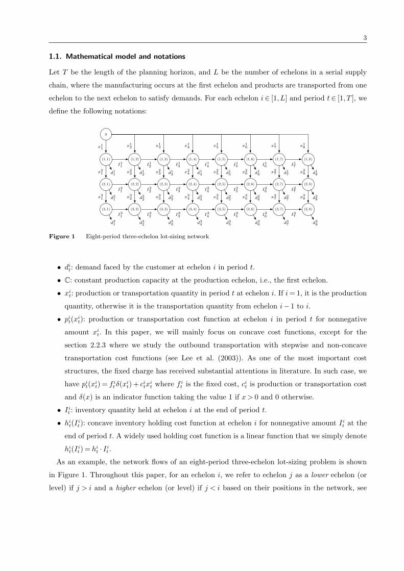
Figure 1 Eight-period three-echelon lot-sizing network

• dit: demand faced by the customer at echelon i in period t.

• C: constant production capacity at the production echelon, i.e., the first echelon.

• xit: production or transportation quantity in period t at echelon i. If i= 1, it is the production

quantity, otherwise it is the transportation quantity from echelon i− 1 to i.

• pit(xit): production or transportation cost function at echelon i in period t for nonnegative

amount xit. In this paper, we will mainly focus on concave cost functions, except for the

section 2.2.3 where we study the outbound transportation with stepwise and non-concave

transportation cost functions (see Lee et al. (2003)). As one of the most important cost

structures, the fixed charge has received substantial attentions in literature. In such case, we

have pit(xit) = f it δ(x

it) + citx

it where f it is the fixed cost, cit is production or transportation cost

and δ(x) is an indicator function taking the value 1 if x> 0 and 0 otherwise.

• I it : inventory quantity held at echelon i at the end of period t.

• hit(I it): concave inventory holding cost function at echelon i for nonnegative amount I it at the

end of period t. A widely used holding cost function is a linear function that we simply denote

hit(Iit) = hit · I it .

As an example, the network flows of an eight-period three-echelon lot-sizing problem is shown

in Figure 1. Throughout this paper, for an echelon i, we refer to echelon j as a lower echelon (or

level) if j > i and a higher echelon (or level) if j < i based on their positions in the network, see

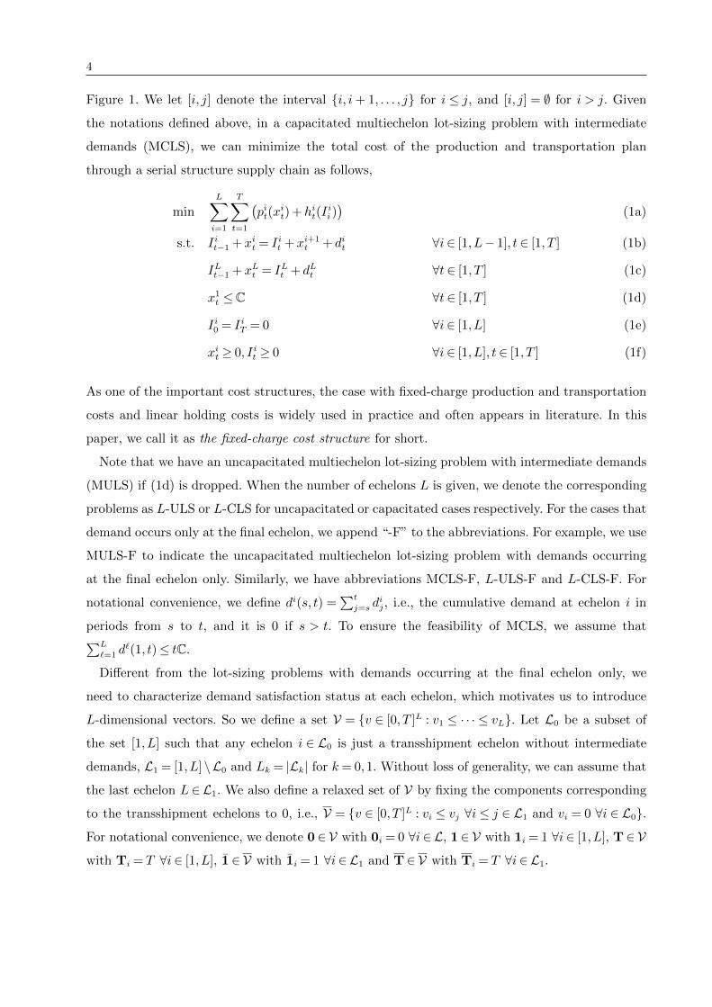
4

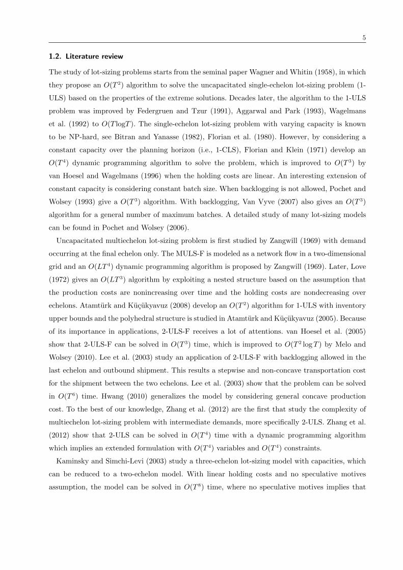
Figure 1. We let [i, j] denote the interval i, i+ 1, . . . , j for i ≤ j, and [i, j] = ∅ for i > j. Given

the notations defined above, in a capacitated multiechelon lot-sizing problem with intermediate

demands (MCLS), we can minimize the total cost of the production and transportation plan

through a serial structure supply chain as follows,

minL∑i=1

T∑t=1

(pit(x

it) +hit(I

ii ))

(1a)

s.t. I it−1 +xit = I it +xi+1t + dit ∀i∈ [1,L− 1], t∈ [1, T ] (1b)

ILt−1 +xLt = ILt + dLt ∀t∈ [1, T ] (1c)

x1t ≤C ∀t∈ [1, T ] (1d)

I i0 = I iT = 0 ∀i∈ [1,L] (1e)

xit ≥ 0, I it ≥ 0 ∀i∈ [1,L], t∈ [1, T ] (1f)

As one of the important cost structures, the case with fixed-charge production and transportation

costs and linear holding costs is widely used in practice and often appears in literature. In this

paper, we call it as the fixed-charge cost structure for short.

Note that we have an uncapacitated multiechelon lot-sizing problem with intermediate demands

(MULS) if (1d) is dropped. When the number of echelons L is given, we denote the corresponding

problems as L-ULS or L-CLS for uncapacitated or capacitated cases respectively. For the cases that

demand occurs only at the final echelon, we append “-F” to the abbreviations. For example, we use

MULS-F to indicate the uncapacitated multiechelon lot-sizing problem with demands occurring

at the final echelon only. Similarly, we have abbreviations MCLS-F, L-ULS-F and L-CLS-F. For

notational convenience, we define di(s, t) =∑t

j=s dij, i.e., the cumulative demand at echelon i in

periods from s to t, and it is 0 if s > t. To ensure the feasibility of MCLS, we assume that∑L

`=1 d`(1, t)≤ tC.

Different from the lot-sizing problems with demands occurring at the final echelon only, we

need to characterize demand satisfaction status at each echelon, which motivates us to introduce

L-dimensional vectors. So we define a set V = v ∈ [0, T ]L : v1 ≤ · · · ≤ vL. Let L0 be a subset of

the set [1,L] such that any echelon i ∈ L0 is just a transshipment echelon without intermediate

demands, L1 = [1,L]\L0 and Lk = |Lk| for k= 0,1. Without loss of generality, we can assume that

the last echelon L∈L1. We also define a relaxed set of V by fixing the components corresponding

to the transshipment echelons to 0, i.e., V = v ∈ [0, T ]L : vi ≤ vj ∀i ≤ j ∈ L1 and vi = 0 ∀i ∈ L0.

For notational convenience, we denote 0∈ V with 0i = 0 ∀i∈L, 1∈ V with 1i = 1 ∀i∈ [1,L], T∈ V

with Ti = T ∀i∈ [1,L], 1∈ V with 1i = 1 ∀i∈L1 and T∈ V with Ti = T ∀i∈L1.

5

1.2. Literature review

The study of lot-sizing problems starts from the seminal paper Wagner and Whitin (1958), in which

they propose an O(T 2) algorithm to solve the uncapacitated single-echelon lot-sizing problem (1-

ULS) based on the properties of the extreme solutions. Decades later, the algorithm to the 1-ULS

problem was improved by Federgruen and Tzur (1991), Aggarwal and Park (1993), Wagelmans

et al. (1992) to O(T logT ). The single-echelon lot-sizing problem with varying capacity is known

to be NP-hard, see Bitran and Yanasse (1982), Florian et al. (1980). However, by considering a

constant capacity over the planning horizon (i.e., 1-CLS), Florian and Klein (1971) develop an

O(T 4) dynamic programming algorithm to solve the problem, which is improved to O(T 3) by

van Hoesel and Wagelmans (1996) when the holding costs are linear. An interesting extension of

constant capacity is considering constant batch size. When backlogging is not allowed, Pochet and

Wolsey (1993) give a O(T 3) algorithm. With backlogging, Van Vyve (2007) also gives an O(T 3)

algorithm for a general number of maximum batches. A detailed study of many lot-sizing models

can be found in Pochet and Wolsey (2006).

Uncapacitated multiechelon lot-sizing problem is first studied by Zangwill (1969) with demand

occurring at the final echelon only. The MULS-F is modeled as a network flow in a two-dimensional

grid and an O(LT 4) dynamic programming algorithm is proposed by Zangwill (1969). Later, Love

(1972) gives an O(LT 3) algorithm by exploiting a nested structure based on the assumption that

the production costs are nonincreasing over time and the holding costs are nondecreasing over

echelons. Atamturk and Kucukyavuz (2008) develop an O(T 2) algorithm for 1-ULS with inventory

upper bounds and the polyhedral structure is studied in Atamturk and Kucukyavuz (2005). Because

of its importance in applications, 2-ULS-F receives a lot of attentions. van Hoesel et al. (2005)

show that 2-ULS-F can be solved in O(T 3) time, which is improved to O(T 2 logT ) by Melo and

Wolsey (2010). Lee et al. (2003) study an application of 2-ULS-F with backlogging allowed in the

last echelon and outbound shipment. This results a stepwise and non-concave transportation cost

for the shipment between the two echelons. Lee et al. (2003) show that the problem can be solved

in O(T 6) time. Hwang (2010) generalizes the model by considering general concave production

cost. To the best of our knowledge, Zhang et al. (2012) are the first that study the complexity of

multiechelon lot-sizing problem with intermediate demands, more specifically 2-ULS. Zhang et al.

(2012) show that 2-ULS can be solved in O(T 4) time with a dynamic programming algorithm

which implies an extended formulation with O(T 4) variables and O(T 4) constraints.

Kaminsky and Simchi-Levi (2003) study a three-echelon lot-sizing model with capacities, which

can be reduced to a two-echelon model. With linear holding costs and no speculative motives

assumption, the model can be solved in O(T 8) time, where no speculative motives implies that

6

it is optimal to transport to the lower echelons as late as possible, i.e., c`t + h`+1t ≥ c`t+1 + h`t in

the case of the fixed-charge cost structure. van Hoesel et al. (2005) provide a detailed analysis of

capacitated multiechelon lot-sizing problem MCLS-F. They show that, in the case of fixed-charge

transportation costs without speculative motives, the MCLS-F can be solved in polynomial time

O(T 7 +LT 4) and the algorithm complexity can be improved to O(T 6) when L= 2. However, they

only provide a pseudo-polynomial algorithm with complexity O(LT 2L+3) for MCLS-F with general

concave costs. Later, this result is largely improved by Hwang et al. (2013) as the MCLS-F is

proved to be polynomial solvable in O(LT 8) time by using a new concept called basis paths.

It is well-known that the lot-sizing problem with concave costs can be seen as a minimal concave

cost network flow problem in a two-dimensional grid with only one source. As much literature

on network flow problems focuses on more general setting where the network could have multiple

sources, we only find two papers, by He et al. (2015) and Ahmed et al. (2016), that are very related

to our work. For more research on general network flow problem, we refer to the literature in those

two papers. He et al. (2015) focus on the grid network with multiple sources at the first level.

They show that MULS, as a special case, is polynomial solvable when the number of echelons L is

fixed but the computational complexity is not specified. Ahmed et al. (2016) study a similar grid

network with flow capacities and classify many NP-hard and polynomial solvable cases. They show

that the minimal concave cost network flow problem in a two-dimensional grid with two sources

at top level is NP-hard. However, the complexity of solving the single source problem, MULS, is

unknown.

1.3. Main contributions and outline

In this paper, our focus is on studying the computational complexity and developing efficient poly-

nomial time algorithms for solving the multiechelon lot-sizing problem with intermediate demands

and production capacity. Our results generalize many previous studies. Because of the interme-

diate demands and production capacity, the problem considered in this paper more practically

formulates actual multiechelon systems and is thus more widely applicable to actual inventory and

supply networks.

Our main contributions are presented in each of the following sections in details and listed as

follows,

• In Section 2.1, we show that the MULS with the fixed-charge cost structure is NP-hard. As

this is a classical single source network flow problem, we establish an important computational

complexity boundary.

• In Sections 2.2 and 2.3, we provide efficient algorithms for solving MULS and MCLS respec-

tively, see Table 1. For the uncapacitated cases, we

7

- in Subsection 2.2.1, generalize the results of Zangwill (1969) to solve the MULS with

general concave costs.

- in Subsection 2.2.2, propose efficient dynamic programming recursions based on shortest

path algorithm to solve the MULS with the fixed-charge cost structure, and an tight

extended formulation with much less variables and constraints than the one suggested by

Zhang et al. (2012).

- in Subsection 2.2.3, extend the dynamic programming recursions in the previous subsec-

tion to solve 2-ULS with backlogging and outbound transportation where the transporta-

tion cost is stepwise and non-concave.

For the capacitated cases, we show that all possible values of cumulative production and

transportation quantities can be enumerated in polynomial time efficiently. Then, following

the approaches by Florian and Klein (1971) and van Hoesel et al. (2005), the application

of all allowable values of cumulative production and transportation quantities gives dynamic

programming recursions to solve MCLS with

- in Subsection 2.3.3, general concave costs, and

- in Subsection 2.3.4, fixed-charge transportation cost without speculative motives.

The computational complexities of all the studied models in this paper are presented in Table

1. It is important to mention that some models are polynomial solvable when L1 is fixed.

Thus, the polynomial solvability depends on the number of echelons with demands instead of

the levels they reside in the supply chain.

• Importantly, we achieve improved complexities in solving several lot-sizing models comparing

the best known algorithms proposed in literature. The comparisons are shown in Table 2.

Except the last row in Table 2, all comparisons are for the cases with demand occurring at

the final echelon only, because our algorithms are general and those models can be solved as

special cases.

In Section 3, we give a family of valid inequalities for MULS. At last, we conclude our paper in

Section 4.

2. Computational complexities

In this section, we prove that MULS is NP-hard and then develop efficient polynomial algorithms

for MULS and MCLS given that the number of echelons is fixed. By considering intermediate

demands, our results (see Table 1) generalize many existing researches, such as Zangwill (1969),

Lee et al. (2003), van Hoesel et al. (2005) and Zhang et al. (2012), which are special cases of our

model. More importantly, we show that the complexities of our algorithms outperform that of

many best known algorithms in literature (see Table 2).

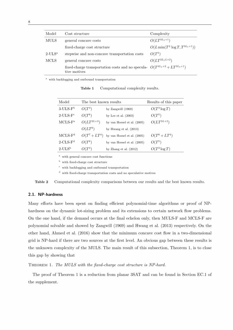
8

Model Cost structure Complexity

MULS general concave costs O(LT 3L1+1)

fixed-charge cost structure O(Lmin(TL logT,T 3L1+1))

2-ULSa stepwise and non-concave transportation costs O(T 5)

MCLS general concave costs O(LT 2L1L+2)

fixed-charge transportation costs and no specula-tive motives

O(T 4L1+2 +LT 3L1+1)

a with backlogging and outbound transportation

Table 1 Computational complexity results.

Model The best known results Results of this paper

3-ULS-Fb O(T 4) by Zangwill (1969) O(T 3 logT )

2-ULS-Fc O(T 6) by Lee et al. (2003) O(T 5)

MCLS-Fa O(LT 2L+3) by van Hoesel et al. (2005) O(LT 2L+2)

O(LT 8) by Hwang et al. (2013)

MCLS-Fd O(T 7 +LT 4) by van Hoesel et al. (2005) O(T 6 +LT 4)

2-CLS-Fd O(T 6) by van Hoesel et al. (2005) O(T 5)

2-ULSb O(T 4) by Zhang et al. (2012) O(T 2 logT )

a with general concave cost functions

b with fixed-charge cost structure

c with backlogging and outbound transportation

d with fixed-charge transportation costs and no speculative motives

Table 2 Computational complexity comparisons between our results and the best known results.

2.1. NP-hardness

Many efforts have been spent on finding efficient polynomial-time algorithms or proof of NP-

hardness on the dynamic lot-sizing problem and its extensions to certain network flow problems.

On the one hand, if the demand occurs at the final echelon only, then MULS-F and MCLS-F are

polynomial solvable and showed by Zangwill (1969) and Hwang et al. (2013) respectively. On the

other hand, Ahmed et al. (2016) show that the minimum concave cost flow in a two-dimensional

grid is NP-hard if there are two sources at the first level. An obvious gap between these results is

the unknown complexity of the MULS. The main result of this subsection, Theorem 1, is to close

this gap by showing that

Theorem 1. The MULS with the fixed-charge cost structure is NP-hard.

The proof of Theorem 1 is a reduction from planar 3SAT and can be found in Section EC.1 of

the supplement.

9

2.2. Uncapacitated cases

In this subsection, we first generalize Zangwill (1969)’s approach on MULS-F to MULS by consider-

ing intermediate demands. Then, we propose a novel algorithm to solve MULS with the fixed-charge

cost structure which outperforms the one suggested by Zhang et al. (2012). At last, we show that

this approach can be extended to solve 2-ULS with backlogging and outbound transportation where

the transportation cost functions are stepwise and non-concave.

2.2.1. General concave costs Following the traditional view by Zangwill (1969), the MULS

with concave cost functions can be seen as a minimal concave flow problem in a two-dimensional

grid. The shipment pattern of any extreme solution can be characterized similarly except satisfying

intermediate demands requires more detailed analysis, which we refer readers to Section EC.2 of

the supplement.

Theorem 2. The MULS with concave cost functions can be solved in O(LT 3L1+1) time.

In the case of MULS-F, we have L1 = 1, so the computation complexity is O(LT 4), which is the

result derived by Zangwill (1969). Theorem 2 indicates that the complexity of MULS depends only

on the number of echelons with demands, regardless of which echelon has demands.

2.2.2. Fixed-charge cost structure As one of the most important cost structures, the

fixed-charge cost structure receives many attentions in literature on studying dynamic lot-sizing

problems. It is well-known that linear holding costs can be dropped and replaced by variable

production and transportation costs because I it =∑t

τ=1(xiτ − xi+1τ ) − di(1, t) ∀i ∈ [1,L − 1] and

ILt =∑t

τ=1 xLτ −dL(1, t). So, in this subsection, we assume that the holding costs are 0 without loss

of generality.

In the case of single-echelon lot-sizing problem with fixed-charge cost structure, the idea of

regeneration points and intervals are used to reformulate the problem as a shortest path problem

on a directed graph. We will generalize regeneration points and intervals to multiechelon lot-sizing

problem as regeneration vectors and arcs, which can be used to reformulate the problem as finding

a shortest path on a directed graph. This novel approach is very different from the traditional

method that considers MULS as a minimal cost network flow on a two-dimensional grid. We show

that the resulting dynamic programming recursions outperform many best known algorithms.

Definition 1. A vector v ∈ [0, T ]L is a regeneration vector if v ∈ V and I ivi = 0 for all i ∈ [1,L].

Let Ai = (v,w) : v,w ∈ V, vj =wj ∀j 6= i and vi <wi for all i ∈ [1,L]. A pair of two regeneration

vectors (v,w) forms a regeneration arc at echelon i with i∈ [1,L], if (v,w)∈Ai.

10

Consider a directed graph G = (V,A), where the arc set A=⋃L

i=1Ai. We define the cost of arc

(v,w)∈Ai for any i∈ [1,L] as

C(v,w) = di(vi + 1,wi)i∑

`=1

c`v`+1 +

f ivi+1 if di(vi + 1,wi) +L∑

`=i+1

d`(1, v`) 6= 0

0 otherwise.

The arc cost includes the production and transportation costs at all the echelons `∈ [1, i] in period

v` + 1 for the demand di(vi + 1,wi), and the fixed cost at echelon i in period vi + 1 if necessary.

The costs can be decomposed into each potential regeneration arc because the variable costs are

additive. One of our main theorems shows that

Theorem 3. The MULS with fixed-charge cost structure can be solved as a shortest path problem

on an acyclic directed graph G = (V,A) with the source node 0 and the sink node T.

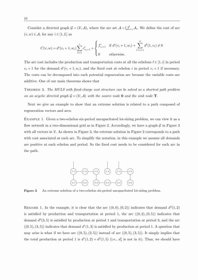
Next we give an example to show that an extreme solution is related to a path composed of

regeneration vectors and arcs.

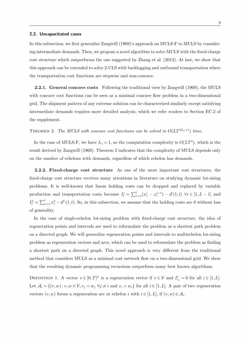
Example 1. Given a two-echelon six-period uncapacitated lot-sizing problem, we can view it as a

flow network in a two-dimensional grid as in Figure 2. Accordingly, we have a graph G in Figure 3

with all vectors in V. As shown in Figure 3, the extreme solution in Figure 2 corresponds to a path

with cost associated at each arc. To simplify the notation, in this example we assume all demands

are positive at each echelon and period. So the fixed cost needs to be considered for each arc in

the path.

(2,1) (2,2) (2,3) (2,4) (2,5) (2,6)

(1,1) (1,2) (1,3) (1,4) (1,5) (1,6)

Figure 2 An extreme solution of a two-echelon six-period uncapacitated lot-sizing problem.

Remark 1. In the example, it is clear that the arc ((0,0), (0,2)) indicates that demand d2(1,2)

is satisfied by production and transportation at period 1, the arc ((0,2), (0,5)) indicates that

demand d2(3,5) is satisfied by production at period 1 and transportation at period 3, and the arc

((0,5), (3,5)) indicates that demand d1(1,3) is satisfied by production at period 1. A question that

may arise is what if we have arc ((0,5), (2,5)) instead of arc ((0,5), (3,5)). It simply implies that

the total production at period 1 is d1(1,2) + d2(1,5) (i.e., d13 is not in it). Thus, we should have

11

(0,0) (0,1) (0,2) (0,3) (0,4) (0,5) (0,6)

(1,1) (1,2) (1,3) (1,4) (1,5) (1,6)

(2,2) (2,3) (2,4) (2,5) (2,6)

(3,3) (3,4) (3,5) (3,6)

(4,4) (4,5) (4,6)

(5,5) (5,6)

(6,6)

d2(1,2)(c11 + c21)+ f21 d2(3,5)(c11 + c23)+ f2

3

d1(1

,3)c

11+

f11

d14 c

14+

f14

d26c

26 + f2

6

d1(5

,6)c

15+

f15

Figure 3 A path in the graph G corresponds to the extreme solution in Figure 2.

a positive production at period 3 to fulfill the demand d13. This solution with arc ((0,5), (2,5))

indicates that after the production at period 1, we hold amount d2(3,5) and transport it until

the period 3. From the discussion, we see that, with arc ((0,5), (2,5)), we still have a feasible

production and transportation plan. However, the solution is not extreme, because I12x

13 > 0 and

the zero inventory ordering property is violated (see Section EC.3 of the supplement). Since the

proof shows that the total cost of a path is equal to the total cost of the corresponding solution,

the shortest path will correspond to an extreme solution with minimal cost.

For a given vector v ∈ V, let G(v) represent the minimum cost of a path in G from v to T. For

notational convenience, we denote vL+1 = T and (v−i, α)∈ V as a vector equal to v except that the

ith component is α. The shortest path algorithm implies

G(v) = minw:(v,w)∈A

C(v,w) +G(w) = mini∈[1,L]:vi<vi+1

minw:(v,w)∈Ai

C(v,w) +G(w) (2)

= mini∈[1,L]:vi<vi+1

minw:w−i=v−i andvi<wi≤vi+1

C(v,w) +G(v−i,wi). (3)

Since (v,w) ∈ A, we know (v,w) ∈ Ai for an i ∈ [1,L]. From the definition of Ai and V, we have

vi+1 = wi+1 ≥ wi > vi. Thus equations (2) and (3) hold. The arc cost C(v,w) equals to a possible

fixed cost plus di(vi + 1, µ)∑i

`=1 c`v`+1, where the fixed cost f ivi+1 occurs if we have production or

transportation at echelon i in period vi+1. Apparently, the fixed cost has to be considered if divi+1 >

0. Otherwise, in the case of divi+1 = 0, we can compare the costs by having G(v) =G(v−i, vi+1) (i.e.,

ignoring the 0 demand) or having production/transportation in period vi + 1 at echelon i. Note

12

that (v−i, vi + 1) ∈ V because vi+1 > vi in (3). Different from the arc cost, here the way of dealing

with fixed cost follows Wagelmans et al. (1992). Therefore, G(v) satisfies a dynamic programming

recursion as follows

G(v) = mini∈[1,L]:vi<vi+1

minvi<λ≤vi+1

[f ivi+1 + di(vi + 1, λ)

i∑`=1

c`v`+1 +G(v−i, λ)

]if divi+1 > 0

min

G(v−i, vi + 1), min

vi<λ≤vi+1

[f ivi+1+

di(vi + 1, λ)i∑

`=1

c`v`+1 +G(v−i, λ)

]if divi+1 = 0.

(4)

Theorem 4. The MULS with fixed-charge cost structure can be solved in

O(min(LT 3L1+1,LTL logT )) time.

Proof For a given i ∈ [1,L] and sub-vector v−i, we can denote G(v−i, ·) as G′(·). Then the

recursion (4) becomes the same 1−dimension recursion as the one by Wagelmans et al. (1992)

(equation (1) in their paper), whose value can be determined in O(logT ) time. Similar results

are obtained by Federgruen and Tzur (1991), Aggarwal and Park (1993). Because G(v) can be

obtained in O(logT ) time with given vector v and index i, the overall complexity is O(LTL logT ).

If L≤ 3L1, this complexity is better than the result in Theorem 2.

Remark 2. By following the traditional network on a two-dimensional grid, the dynamic recur-

sions developed in Melo and Wolsey (2010) and Zhang et al. (2012) consider the regeneration

points one echelon after another. Distinct from the traditional approach, our algorithm is to find a

shortest path on an L-dimensional graph with node set V such that a node on the shortest path is

a regeneration vector which has regeneration points at each echelon as its components. The novel

approach allows us to determine the optimal solutions more efficiently. As evidences of the efficacy

of our algorithm, Theorem 4 suggests improved complexities than Zangwill (1969)’s for 2-ULS-F

and 3-ULS-F, and Zhang et al. (2012)’s for 2-ULS (the complexity comparisons are shown in Table

2). An interesting observation is that the intermediate demands may have no effect on the com-

plexity for 2-ULS, because we have shown the complexity for 2-ULS is O(T 2 logT ) and the best

known complexity for 2-ULS-F is also O(T 2 logT ) by Melo and Wolsey (2010).

2.2.3. Backlogging and outbound transportation The efficiency of our algorithm in Sec-

tion 2.2.2 relies on the fact that, without considering the fixed-charge, the production and trans-

portation costs are linear and additive. Hence the total cost can be decomposed into the cost of

each arc. Such property usually does not hold for general cost structures. However, if the cost

functions lead to an enumeration of demand units over a set within a reasonable size, then the pro-

posed dynamic programming recursions in Section 2.2.2 can still be applied to achieve an efficient

algorithm.

13

We consider a 2-ULS with backlogging and outbound transportation, which is studied by Lee

et al. (2003) to consolidate outbound transportation scheduling from a third-party warehouse

(TPW) to a group of downstream distribution centers (DC). The outbound transportation cost

from the TPW consists of a fixed cost and a per-cargo cost. Because of the cargo capacity, the

transportation cost follows a stepwise function, which is non-concave. The TPW has the option of

releasing an outbound transportation earlier or later than it is actually needed at the DC at the

expense of inventory holding or customer waiting cost. The problem can be formulated as follows,

minn∑t=1

(p1t (x

1t ) + p2

t (x2t ) +h2

t I2t +w2

t I−t

)(5a)

s.t. I1t−1 +x1

t = I1t +x2

t + d1t ∀t= 1, . . . , T (5b)

(I2t−1− I−t−1) +x2

t = (I2t − I−t ) + d2

t ∀t= 1, . . . , T (5c)

I i0 = I in = I−0 = I−n = 0 ∀i= 1,2 (5e)

xit ≥ 0, I it ≥ 0, I−t ≥ 0 ∀i= 1,2, t= 1, . . . , T (5f)

where the constraint (5c) models the backlogs and variable I−t indicates backlogging quantities in

period t. In the model, for all periods t∈ [1, T ], we have the fixed-charge production costs p1t (x

1t ) =

f1t δ(x

1t ) + c1

tx1t , the transportation costs p2

t (x2t ) = f2

t δ(x2t ) + c2

tx2t +Adx

2tWe, where A is the cost of

delivering a cargo and W is the capacity of each cargo, inventory holding cost h2t and customer

waiting cost w2t . Our model generalizes the one proposed by Lee et al. (2003) since ours includes the

variable costs of production and transportation, and intermediate demands. Note that the linear

inventory holding costs of I1t at the first echelon are omitted without loss of generality because

I1t =

∑t

τ=1(x1τ − x2

τ ). Lee et al. (2003) show that an optimal solution can be obtained in O(T 6)

time for the case that demand is occurring at the final echelon only. The main contribution in this

subsection is that we are able to obtain an optimal solution in O(T 5) time even with intermediate

demands.

Let Q(t, s1, β1), for all t, s1 ∈ [1, T ] and 0≤ β1 ≤ d2s1

, be the minimal cost of satisfying

• the demands in periods t through T at echelon 1 (i.e., d1t , . . . , d

1T );

• d2s1−β1 unit of demand in period s1 plus the demands in periods s1 + 1 through T at echelon

2 (i.e., d2s1+1, . . . , d

2T )

by productions from period t to T . We have boundary condition Q(T + 1, T, d2T ) = 0. The 2-ULS

with backlogging and outbound transportation is solved by finding Q(1,1,0). Note that we could

have s1 < t, which indicates that the demand in period s1 at echelon 2 is backlogged. Lee et al.

(2003) show that, due to the optimality property, the choices of (s1, β1) can be limited into a set,

denoted as Γ, with its size of O(T 2).

14

First we have a dynamic recursion when (s1, β1) 6= (T,d2T ),

Q(t, s1, β1) = min(s2,β2)∈Γ∗

Q(t, s2, β2) + g(s1, β1;s2, β2) + c1t · (d2(s1, s2− 1) +β2−β1) (6)

where Γ∗ = (s2, β2)∈ Γ : s2 ≥max(s1, t) and β2 >β1 if s2 = s1,• in the definition of Γ∗, s2 ≥ t is required because the backorders from period s1 to t− 1 at

echelon 2 are satisfied by a single transportation (follow the Property 2 and 3 in Lee et al.

(2003)). It is obvious that we need s2 ≥ s1 and β2 >β1 if s2 = s1.

• g(s1, β1;s2, β2) is the minimal total cost of satisfying

- d2s1−β1 unit of demand in period s1 at echelon 2;

- the demands in periods s1 + 1 through s2− 1 at echelon 2; and

- β2 unit of demand in period s2 at echelon 2,

i.e., the total demand is d2s1− β1 + d2(s1 + 1, s2 − 1) + β2 = d2(s1, s2 − 1) + β2 − β1, such that

the solution to g(s1, β1;s2, β2) has no regeneration point at the second echelon from period s1

to s2− 1 if β1 <ds1 and from period s1 + 1 to s2− 1 if β1 = ds1 .

• the last term of the recursion indicates the variable production cost in period t for satisfying

demands d2(s1, s2− 1) +β2−β1 that is transported to the second echelon.

Apparently, the recursion (6) is not enough to obtain the value of Q(1,1,0) since it only works on

satisfying demands d2(s1, s2− 1) + β2− β1 at echelon 2 from a given production period t. That is

also the reason why the recursion (6) is not necessary when (s1, β1) 6= (T,d2T ). The next recursion

links two production periods t and t′

Q(t, s1, β1) = mint′∈∆t,s1,β1

Q(t′, s1, β1) +

0 if (s1, β1) = (1,0)

f1t + c1

t · d1(t, t′− 1) otherwise.(7)

where ∆t,s1,β1= t′ ∈ [t + 1, T + 1] : t ≤ T when (s1, β1) 6= (T,d2

T ). In the definition of ∆t,s1,β1,

t′ = T + 1 only if (s1, β1) = (T,d2T ) and when t′ = T + 1 it invokes the boundary condition Q(T +

1, T, d2T ) = 0. For example, Q(t, T, d2

T ) =Q(T + 1, T, d2T ) + f1

t + c1t · d1(t, T ) indicates that period t

is the final period with positive productions and Q(t, T, d2T ) is the cost of fulfilling demands from

period t to period T at echelon 1. The recursion (6) needs to be applied afterward to figure out

how many demands at echelon 2 may be satisfied by the production in period t. The condition

(s1, β1) = (1,0) in the recursion (7) indicates that we could have G(1,1,0) = G(t′,1,0) for some

period t′ such that the demands from period 1 to t′ − 1 at the second echelon are satisfied by

backlogging with production in period t′. It is clear that we should take the minimal value of those

two recursions. In summary, we have

Q(t, s1, β1) = min

min(s2,β2)∈Γ∗

Q(t, s2, β2) + g(s1, β1;s2, β2)

+ c1t · (d2(s1, s2− 1) +β2−β1) if (s1, β1) 6= (T,d2

T )

mint′∈∆t,s1,β1

Q(t′, s1, β1) +

0 if (s1, β1) = (1,0)

f1t + c1

t · d1(t, t′− 1) otherwise.

15

Suppose that the values of all g(s1, β1;s2, β2) are given. The recursion (6) can be evaluated in

constant time with the given t, (s1, β1), (s2, β2), and (7) can be evaluated in constant time with

the given t, (s1, β1), t′. Thus, it would be possible to solve the problem in O(T 5) time. We point

out that the above dynamic programming recursions follow the same idea as the recursions (4) in

Section 2.2.2, except that, in the recursion (4), we know the demand in each period is fully satisfied

when cost functions are concave, hence the parameter β1 is unnecessary.

Note that g(s1, β1;s2, β2) is similar to the customer subproblem defined by Lee et al. (2003),

except that it is independent of any production period. Following a similar approach, we can show

that the values of all g(s1, β1;s2, β2) can also be obtained in O(T 5) time as well (see Section EC.4

of the supplement). Therefore, we have

Theorem 5. The 2-ULS with backlogging and outbound transportation can be solved in O(T 5)

time.

2.3. Capacitated cases

Capacitated lot-sizing problems are usually much more complicated than their uncapacitated coun-

terparts mainly due to the reason that the zero inventory ordering property does not hold after

imposing a capacity. However, starting from Florian and Klein (1971), many researchers find that

the production and transportation quantities could be enumerated in polynomial time if the capac-

ity is stationary. van Hoesel et al. (2005) provide a detailed study on capacitated multiechelon

lot-sizing problem with demand occurring at the final echelon only. They show that, in the view of

the network flow problem, the flow corresponding to any extreme solution can be decomposed into

a sequence of the so-called subplans, where each subplan has at most one positive production arc

strictly less than the capacity. This property of the subplan allows them to enumerate all possible

values of cumulative production and transportation quantities in each subplan. Then, they are able

to solve MCLS-F through a two-phase dynamic programming by considering adjacent subplans.

A more general approach is proposed in this subsection to solve MCLS. More specifically, the

definition of a subplan needs to be adjusted because of the intermediate demands. It also turns

out that, in our case, the cumulative production and transportation quantities have a much richer

structure. By enumerating all allowable values, we are able to solve MCLS in O(LT 2L1L+2) time for

general concave costs, which outperforms the one proposed by van Hoesel et al. (2005) for solving

MCLS-F. Throughout this section, for two L-dimensional vectors u, v, we denote u≤ v if u` ≤ v`∀` ∈ [1,L] component-wise. Similarly, min(u, v) is a L-dimensional vector whose `th component

equals to min(u`, v`) ∀`∈ [1,L]. We define Di(v, w) =∑L

`=i d`(v` + 1, w`) ∀i∈ [1,L].

16

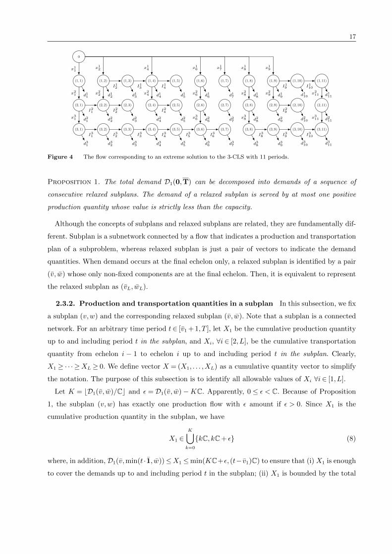
2.3.1. Subplans and relaxed subplans We consider flow in the network corresponding to

any extreme point, where the network consists of nodes (i, t) with echelon i and period t, see

Figure 4. After removing all production arcs, the network is decomposed into several connected

components. Then, we connect each isolated node without demand to the node on its left (con-

necting to its above node if the node is in period 1), and define each connected component as a

subplan (v,w) with v,w ∈ V and v ≤ w if it includes nodes (i, vi + 1), . . . , (i,wi) ∀i ∈ [1,L] where

vi+1 ≤wi for i= 1, . . . ,L− 1. We also require that, for any j ∈ [1,L− 1], we have either vj+1 <wj

or v` = w` ∀` ∈ [j + 1,L], because of the arborescent structure of an extreme solution in the sub-

plan. Note that if vj+1 ≥wj, then, in the subplan, there is no flow that can connect to the nodes

(j + 1, vj+1 + 1), . . . , (j + 1,wj+1). Hence, the subplan only contains nodes at echelons 1, . . . , j and

we need to have v` = w` ∀` ∈ [j + 1,L]. We say two subplans (v′,w′) and (v′′,w′′) are consec-

utive if w′ = v′′. For example, in Figure 4, if d17 > 0, then we have three consecutive subplans

((0,0,0), (6,7,7)), ((6,7,7), (7,7,7)) and ((7,7,7), (11,11,11)), otherwise we only have two consec-

utive subplans ((0,0,0), (7,7,7)) and ((7,7,7), (11,11,11)). As common in network flow problems,

we define an arc as free if it carries an amount of flow that is both positive and strictly less than

its capacity. Because the flow corresponding to the extreme solution is acyclic, there is at most one

free production arc entering the subplan.

The definition of the subplan is first introduced by van Hoesel et al. (2005) except that

their requirement is vi+1 < wi ∀i ∈ [1,L − 1] for a subplan (v,w). For example, in Figure 4,

((6,7,7), (7,7,7)) is not a valid subplan anymore because v2 =w1 = 7. Thus, we have only two con-

secutive subplans ((0,0,0), (7,7,7)) and ((7,7,7), (11,11,11)) when d17 > 0. Apparently, we could

have two free production arcs, for example x14 and x1

7, in the subplan ((0,0,0), (7,7,7)). The exam-

ple shows that, with the requirements vi+1 <wi ∀i ∈ [1,L− 1] in the case of having intermediate

demands, we cannot assure that there is at most one free production arc entering each subplan,

which is the key property we need for subplans. Therefore, we use a different (relaxed) requirement

in our subplan definition, which allows a subplan to contain only nodes at some higher levels, such

as the subplan ((6,7,7), (7,7,7)).

In summary, any extreme solution can be decomposed into a sequence of consecutive subplans

and there is at most one free production arc entering the subplan. Even though we need two vectors

v,w ∈ V for a subplan, the total demand of a subplan depends only on v, w ∈ V where v` = v` and

w` = w` ∀` ∈ L1. So we define the pair (v, w) as a relaxed subplan. We know that the subplan

(v,w) satisfies, for any j ∈ [1,L−1], either vj+1 <wj or v` =w` ∀`∈ [j+1,L]. It implies that (v, w)

satisfies, for any j ∈ [1,L−1]∩L1, either vj+1 <wj or v` =w` ∀`∈ [j+ 1,L]. Similarly, two relaxed

subplans (v′, w′) and (v′′, w′′) are consecutive if w′ = v′′. Based on the above discussions, we have

17

0

(1,1)

d11

(1,2)

d12

(1,3)

d13

(1,4)

d14

(1,5)

d15

(1,6)

d16

(1,7)

d17

(1,8)

d18

(1,9)

d19

(1,10)

d110

(1,11)

d111

(2,1)

d21

(2,2)

d22

(2,3)

d23

(2,4)

d24

(2,5)

d25

(2,6)

d26

(2,7)

d27

(2,8)

d28

(2,9)

d29

(2,10)

d210

(2,11)

d211

(3,1)

d31

(3,2)

d32

(3,3)

d33

(3,4)

d34

(3,5)

d35

(3,6)

d36

(3,7)

d37

(3,8)

d38

(3,9)

d39

(3,10)

d310

(3,11)

d311

x11x12 x14 x16 x17 x18 x19

I12 I13 I14 I19 I110

x21 x22 x24 x26 x28 x29 x211

I21 I22 I24 I29

x31 x36 x38 x311

I31 I32 I33 I34 I35 I36 I38 I39 I310

Figure 4 The flow corresponding to an extreme solution to the 3-CLS with 11 periods.

Proposition 1. The total demand D1(0,T) can be decomposed into demands of a sequence of

consecutive relaxed subplans. The demand of a relaxed subplan is served by at most one positive

production quantity whose value is strictly less than the capacity.

Although the concepts of subplans and relaxed subplans are related, they are fundamentally dif-

ferent. Subplan is a subnetwork connected by a flow that indicates a production and transportation

plan of a subproblem, whereas relaxed subplan is just a pair of vectors to indicate the demand

quantities. When demand occurs at the final echelon only, a relaxed subplan is identified by a pair

(v, w) whose only non-fixed components are at the final echelon. Then, it is equivalent to represent

the relaxed subplan as (vL, wL).

2.3.2. Production and transportation quantities in a subplan In this subsection, we fix

a subplan (v,w) and the corresponding relaxed subplan (v, w). Note that a subplan is a connected

network. For an arbitrary time period t∈ [v1 + 1, T ], let X1 be the cumulative production quantity

up to and including period t in the subplan, and Xi, ∀i ∈ [2,L], be the cumulative transportation

quantity from echelon i − 1 to echelon i up to and including period t in the subplan. Clearly,

X1 ≥ · · · ≥XL ≥ 0. We define vector X = (X1, . . . ,XL) as a cumulative quantity vector to simplify

the notation. The purpose of this subsection is to identify all allowable values of Xi ∀i∈ [1,L].

Let K = bD1(v, w)/Cc and ε = D1(v, w)−KC. Apparently, 0 ≤ ε < C. Because of Proposition

1, the subplan (v,w) has exactly one production flow with ε amount if ε > 0. Since X1 is the

cumulative production quantity in the subplan, we have

X1 ∈K⋃k=0

kC, kC+ ε (8)

where, in addition, D1(v,min(t · 1, w))≤X1 ≤min(KC+ε, (t− v1)C) to ensure that (i) X1 is enough

to cover the demands up to and including period t in the subplan; (ii) X1 is bounded by the total

18

capacities in periods from v1 + 1 to t and the total demands in the subplan. Next, we introduce

Proposition 2 to characterize the possible values for the transportation quantities Xi for a given

i∈ [2,L].

Proposition 2. The cumulative transportation quantities Xi with i ∈ [2,L] have three allowable

forms as follows,

Form (1): there exist j1 ∈ [i − 1,L − 1], µ10 ∈ [0,K], µ1

` ∈ [v` + 1,w`] ∀`[1, j1] and η1` ∈ [v` + 1,w`]

∀`∈ [i, j1] such that

Xi = Y (µ10)−

i−1∑`=1

d`(v` + 1, µ1`)−

j1∑`=i

d`(η1` , µ

1`).

Form (2): there exist j2 ∈ [i − 1,L − 1], µ20 ∈ [0,K], µ2

` ∈ [v` + 1,w`] ∀`[1, j2] and η2` ∈ [v` + 1,w`]

∀`∈ [i, j2] such that

Xi = Y (µ20)−

i−1∑`=1

d`(v` + 1, µ2`) +

j2∑`=i

d`(η2` , µ

2`).

Form (3): there exist µ3` ∈ [v` + 1,w`] ∀`∈ [i,L] such that

Xi =L∑`=i

d`(v` + 1, µ3`),

where Y (τ)∈ τC, τC+ ε.

Here, we make a few comments on the proposition: 1). When demand occurs only at the final

echelon, Forms (1) and (2) degenerate to Xi = Y (τ) for some τ ∈ [0,K]. Together with Form (3),

Proposition 2 is equivalent to the result shown by van Hoesel et al. (2005). Therefore, Proposition

2 generalizes the results for MCLS-F. 2). The most important property of Xi shown by Proposition

2 is that, in Forms (1) and (2), besides the total production quantity of an initial sequence of

production periods minus the demands of an initial sequence of periods at each above level, i.e.,

Y (µ10)−

i−1∑`=1

d`(v` + 1, µ1`) or Y (µ2

0)−i−1∑`=1

d`(v` + 1, µ2`),

the value of Xi can be characterized by the demands in some periods at echelon i, . . . , j1(j2) where

(a) j1(j2)<L; (b) those periods in each echelon are consecutive. 3). We give two examples on Forms

(1) and (2). For example, in subplan ((0,0,0), (6,7,7)) of Figure 4, the cumulative transportation

quantity up to period 2 at echelon 2, x21 + x2

2, equals to the production up to period 5, i.e., x11 +

x12 +x1

4, minus an initial sequence of demand periods d1(1,5), and further minus demand d2(4,5),

as described in Form (1). Another example is in subplan ((7,7,7), (11,11,11)), the cumulative

transportation quantity up to period 9 at echelon 2, x28 +x2

9, is equal to the production up to period

8 in the subplan, i.e., x18, minus an initial sequence of demand periods d1(8,8), and further plus

demand d2(9,10), as described in Form (2).

19

In addition, we require Di(v,min(t · 1, w))≤Xi ≤Xi−1 − di−1(vi−1 + 1,min(t, wi−1)) ∀i ∈ [2,L],

and Xi = 0 when t≤ vi ∀i∈ [2,L]∩L1 to ensure that 1). the demands are satisfied on time, 2). the

quantity Xi−1 is used to first satisfy demands at echelon i− 1 up to and including period t in the

subplan, then the part of it is transported to the next echelon i, and 3). the transportation is in

the relaxed subplan at echelons with intermediate demands. Because there is no demand at any

echelon in L0, only the pair (v, w) representing relaxed subplan matters in defining Xi ∀i ∈ [1,L].

Therefore, all allowable values of X depend on t, v and w, and we define

Definition 2. Let Θt,(v,w) be the set of all allowable values of X in the subplan (v,w).

Remark 3. We can summarize the complexity of allowable values for X ∈Θt,(v,w) as follows. The

number of allowable values for X1 is in O(T ) because it depends on K and K ≤ T . The complexity of

the number of allowable values for Xi ∀i∈ [2,L] depends on the number of parameters and the size

of the intervals [v`+1,w`] ∀`∈L1 in Proposition 2. The number of parameters needed for Form (3)

is |L1∩ [i,L]|. The number of parameters needed for Form (1) is 1 + |L1∩ [1, i−1]|+ 2|L1∩ [i, j1]| ≤

L1 + |L1 ∩ [i,L − 1]| because j1 < L. We have the same result for Form (2). So, the number of

allowable values for Xi for each i ∈ [2,L] is in O(TL1+|L1∩[i,L−1]|) or O(T 2L1) if relaxing further.

From the discussion above, it is easy to calculate that the number of allowable values for X is

O(T 1+2L1(L−1)).

2.3.3. General concave costs Given a relaxed subplan (v, w), we define φ(v,w)(t,X), with a

time period t ∈ [v1, T ] and cumulative quantity vector X ∈Θt,(v,w), as the the optimal cost where

the demand D1(0, v) is satisfied, plus the optimal cost of having X1 as the cumulative production

quantity up to and including period t in the subplan, and Xi, ∀i ∈ [2,L], as the cumulative trans-

portation quantity from echelon i− 1 to echelon i up to and including period t in the subplan. We

also require that t ·C ≥ D1(0, v) because the demand D1(0, v) has been satisfied. The goal is to

determine the value of φ(T,T)(T,0).

Note that φ(v,w)(t,0) is simply the optimal cost of satisfying the demand D1(0, v), and

φ(v,w)(t,D1(v, w) ·1) is the optimal cost of satisfying the demand D1(0, w). So, we have

φ(v,w)(t,0) = φ(u,v)(t,D1(u, v) ·1), (9)

for any relaxed subplan (u, v) with u≤ v. Note that (9) implies that t ·C≥D1(0, v). We also give

boundary conditions φ(0,0)(0,0) = 0. With this boundary conditions and (9), we have φ(0,w)(0,0) = 0

∀w ∈ V.

Suppose that we have φ(v,w)(t−1,X) with X ∈Θt−1,(v,w), i.e., X is a cumulative quantity vector

up to and including period t−1 in the same relaxed subplan. Then, at echelon i∈ [1,L] in period t,

the production quantity is Xi−X i and the inventory quantity is Xi−Xi+1−di(vi + 1,min(t, wi)),

20

except that, at echelon L, the inventory quantity is XL− dL(vL + 1,min(t, wL)). Apparently, X1−X1 ∈ 0, ε,C and Xi ≥X i ∀i∈ [2,L]. So, we have recursion

φ(v,w)(t,X) = minX∈Θt−1,(v,w)(X)

φ((v,w)(t− 1,X) +L∑i=1

pit(Xi−X i)

+L−1∑i=1

hit(Xi−Xi+1− di(vi + 1,min(t, wi))) +hLt (XL− dL(vL + 1,min(t, wL))) (10)

where Θt−1,(v,w)(X) = X ′ ∈Θt−1,(v,w) :X1−X ′1 ∈ 0, ε,C,Xi ≥X ′i ∀i∈ [2,L]. The MCLS can be

solved by recursion (9), (10) and boundary conditions φ(0,0)(0,0) = 0.

Recall that Remark 3 indicates that the number of allowable values for X is in O(T 1+2L1(L−1)).

With the given v, w, t, the recursion (9) can be evaluated in O(TL1) time because of u, and di(vi +

1,min(t, wi)) ∀i∈ [1,L] can be evaluated in O(L). Thus, the total time that recursion (9) needs is

in O(T 3L1+1). If X and X are given as well, then recursion (10) can be evaluated in O(L) time.

With observation that X −X ∈ 0, ε,C and simple calculations, we can evaluate the recursion

(10) in O(LT 4L1L+2L1+3) time. Thus, MCLS can be solved in polynomial time when L is fixed.

The relations between X and X can be explored further as they are cumulative quantity vectors

up to two adjacent time periods in the same relaxed subplan. This can lead to a more efficient

evaluation of the recursion (10) with a complexity of O(LT 2L1L+2). Let Θ2t,(v,w) be the set including

all allowable values of pairs (X,X). We have

Proposition 3. The number of allowable values in Θ2t,(v,w) is in O(T 2L1(L−1)+1).

The recursion (10) can be evaluated in O(L) time with given v, w, t, and (X,X)∈Θ2t,(v,w). Thus,

the complexity is O(LT 2L1+1+2L1(L−1)+1) = O(LT 2L1L+2). We define Θ2t,(v,w)(X) as the collection

of all the allowable values of X with (X,X) ∈Θ2t,(v,w). Summarizing all the discussions above, we

have the following theorem.

Theorem 6. The MCLS can be solved by dynamic programming recursions as follows,

φ(v,w)(t,X) = minX∈Θ2

t,(v,w)(X)

φ((v,w)(t− 1,X) +L∑i=1

pit(Xi−X i)

+L−1∑i=1

hit(Xi−Xi+1− di(vi + 1,min(t, wi))) +hLt (XL− dL(vL + 1,min(t, wL))) (11)

with boundary conditions φ(v,w)(t,0) = φ(u,v)(t,D1(u, v) · 1) ∀u≤ v and relaxed subplan (u, v), and

φ(0,0)(0,0) = 0, where the recursions (11) can be performed in O(LT 2L1L+2) time.

Remark 4. For 1-CLS, we have L = L1 = 1. Theorem 6 implies the same complexity O(T 4) as

Florian and Klein (1971). In the case of 2-CLS-F, i.e., L = 2 and L1 = 1, Theorem 6 indicates

that the model can be solved in O(T 6) time which improves the complexity O(T 7) proposed by

van Hoesel et al. (2005).

21

2.3.4. Fixed-charge transportation costs without speculative motives The assump-

tion of no speculative motives is commonly assumed for the production and inventory holding

costs in traditional economic lot-sizing models and appears in a lot of literature. In the context of

fixed-charge transportation costs, no speculative motives indicates that it is attractive to transport

as late as possible. More formally, c`t +h`+1t ≥ c`t+1 +h`t if inventory holding cost is linear. With the

same arguments by van Hoesel et al. (2005), there exists an optimal solution satisfying the zero

inventory ordering (ZIO) property, i.e., I it−1xit = 0 for i∈ [1,L] and t∈ [1, T ], because of fixed-charge

transportation costs and no speculative motives. Therefore, we can limit ourselves on the extreme

solutions with ZIO property. The MCLS can be solved by decoupling the production echelon (the

first echelon) from the rest of the model and the echelon from level 2 to level L can be solved

by using dynamic programming recursions in Section 2.2.1 due to ZIO property. Note that the

production costs and inventory holding costs are still assumed to be generally concave. We have

Theorem 7. The MCLS with fixed-charge transportation costs and no speculative motives can be

solved in O(T 4L1+2 +LT 3L1+1).

Corollary 1. The 2-CLS-F with fixed-charge transportation costs and no speculative motives can

be solved in O(T 5).

Remark 5. Theorem 7 is different from Theorem 6 that it shows a complexity which is indepen-

dent to the number of echelon L. Under the condition of fixed-charge transportation costs with no

speculative motives, the MCLS can be solved within polynomial time when L1 is fixed. Together

with Corollary 1, they generalize and outperform the complexity O(T 7 + LT 4) for MCLS-F, i.e.

L1 = 1, and O(T 6) for 2-CLS-F by van Hoesel et al. (2005).

3. Multiechelon Inequalities

In this section, we study MULS with fixed-charge cost structure (MULS for simplification) as

follows

minL∑i=1

T∑t=1

(citx

it + f ity

iat

)(12a)

s.t.T∑t=1

xit =L∑`=i

d`(1, T ) ∀i∈ [1,L] (12b)

t∑j=1

(xij −xi+1j )≥ di(1, t) ∀i∈ [1,L− 1], t∈ [1, T ] (12c)

t∑j=1

xLj ≥ dL(1, t) ∀t∈ [1, T ] (12d)

22

x1t ≤

L∑`=1

d`(t, T )y1t ∀t∈ [1, T ] (12e)

xit ≥ 0, yit ∈ 0,1 ∀i∈ [1,L], t∈ [1, T ] (12f)

where binary variables yit ∀i ∈ [1,L], t ∈ [1, T ] are introduced to model the fixed-charge costs. Fol-

lowing Theorem 3, we have an extended formulation for MULS with variables 0 ≤ γv,w ≤ 1 to

indicate the flow on arc (v,w)∈A.

min∑

(v,w)∈A

C(v,w)γ(v,w)

s.t∑

v:(v,w)∈A

γ(v,w)−∑

v:(w,v)∈A

γ(w,v) =

−1 if v=T

1 if v= 0

0 otherwise

0≤ γ(v,w) ≤ 1 ∀(v,w)∈A

xit =L∑`=i

∑(v,w)∈A`:vi=t

d`(v` + 1,w`)γ(v,w) ∀i∈ [1,L], t∈ [1, T ]

yit =∑

(v,w)∈Ai:vi=t

γ(v,w) ∀i∈ [1,L], t∈ [1, T ].

Considering that there are O(TL) nodes and O(LTL+1) arcs in the graph G, we have the following

corollary.

Proposition 4. The MULS has an extended formulation with O(LTL+1) variables and O(TL)

constraints.

Note that the proposed extended formulation has less variables and constraints than the one

in Zhang et al. (2012). We give a family of valid inequalities for MULS, which generalizes many

known results.

Theorem 8. For 0 = k0 ≤ k1 ≤ · · · ≤ kL ≤ n, let [ki−1 + 1, ki]⊆ Ti ⊆ [1, ki] and Si ⊆ Ti ∀i ∈ [1,L].

We have L-echelon inequality

L∑i=1

∑t∈Ti\Si

xit +∑t∈Si

φityit

≥ L∑i=1

di(1, ki) (13)

where

φit =L∑`=i

d`(αi`t + 1, βi`t) (14)

such that αiit = t− 1, βiit = maxτ ≥ t− 1 : [t, τ ]⊆ Ti,

αi`t = maxτ ≥ αi`−1,t : [αi`−1,t + 1, τ ]⊆ T` and βi`t = maxτ ≥ βi`−1,t : [βi`−1,t + 1, τ ]⊆ T`

for `∈ [i+ 1,L].

23

Remark 6. In the definition of αi`t and βi`t, we have αi`t = αi`−1,t when αi`−1,t + 1 /∈ T`, and βi`t =

βi`−1,t when βi`−1,t + 1 /∈ T`. In general, we have βi`t ≤ k` ∀` ∈ [i,L]. The equality holds when

Ti = [1, ki] since βiit = maxτ ≥ t− 1 : [t, τ ] ⊆ Ti = ki. Then, βi`t = k` ∀` ∈ [i+ 1,L] follows by its

iterative definition and the fact that [k`−1 + 1, k`]⊆ T` ∀`∈ [i+ 1,L].

If 0 = k0 = k1 = · · ·= kL−1 ≤ kL ≤ n, then we have Ti = Si = ∅ ∀i∈ [1,L−1] and SL ⊆ TL = [1, kL].

It is easy to calculate that αLL,t = t− 1 and βLL,t = kL. So the inequality (13) becomes∑t∈[1,kL]\SL

xLt +∑t∈SL

dL(t, kL)yLt ≥ dL(1, kL)

which is the (`,S) inequality of Barany et al. (1984).

If 0 = k0 = k1 = · · · = kL−2 ≤ kL−1 ≤ kL ≤ n, then we have Ti = Si = ∅ ∀i ∈ [1,L − 2], SL−1 ⊆

TL−1 = [1, kL−1], SL ⊆ TL and [kL−1, kL]⊆ TL ⊆ [1, kL]. It is easy to get that αL−1L−1,j = αLL,t = t− 1,

αL−1L,t = βLL,t = maxτ ≥ t − 1 : [t, τ ] ⊆ TL, βL−1

L−1,t = kL−1 and βL−1L,t = kL. So the inequality (13)

becomesL∑

i=L−1

∑t∈Ti\Si

xit +∑t∈Si

φityit

≥ L∑i=L−1

di(1, ki)

where φL−1t = dL−1(t, kL−1) + dL(t, kL) − dL(t, βLL,t) and φLt = dL(t, βLL,t), which is the 2-echelon

inequality of Zhang et al. (2012).

Zhang et al. (2012) show the hierarchy of formulations for 2-ULS. The result can be easily

extended to MULS except the shortest path based extended formulation is the strongest one.

4. Conclusions

We study the multiechelon lot sizing with intermediate demands (MLS). Many existing studies

have provided polynomial algorithms on MLS with demand occurring at the final echelon only,

or shown that multiple sources network flow problem is NP-hard. However, the complexity of

MLS with the fixed-charge cost structure, which is a classical single source network flow problem,

remains unknown. As one of many contributions in this paper, we prove that the MLS with the

fixed-charge cost structure is NP-hard and close the theoretical gap.

We investigate both uncapacitated and capacitated MLS with different types of cost functions,

such as the general concave costs, the fixed-charge cost structure, stepwise and non-concave trans-

portation cost, and fixed-charge transportation cost with no speculative motives. By considering

intermediate demands, our results (see Table 1) generalize many existing researches, such as Zang-

will (1969), Lee et al. (2003) and van Hoesel et al. (2005), which are special cases of the problems

studied in this paper. In addition to developing efficient algorithms for solving both MULS and

MCLS, we show that the complexities of our algorithms outperform that of many best known

algorithms in literature (see Table 2).

24

References

Aggarwal A, Park J (1993) Improved algorithms for economic lot size problems. Operations Research

41(3):549–571.

Ahmed S, He Q, Li S, Nemhauser G (2016) On the computational complexity of minimum-concave-cost flow

in a two–dimensional grid. Accepted by SIAM Journal on Optimization .

Ahuja R, Magnanti T, Orlin J (1993) Network Flows: Theory, Algorithm, and Applications (Englewood

Cliffs, NJ: Prentice Hall).

Atamturk A, Kucukyavuz S (2005) Lot sizing with inventory bounds and fixed costs: Polyhedral study and

computation. Operations Research 53(4):711–730.

Atamturk A, Kucukyavuz S (2008) An O(n2) algorithm for lot sizing with inventory bounds and fixed costs.

Operations Research Letters 36(3):297–299.

Barany I, van Roy T, Wolsey L (1984) Uncapacitated lot-sizing: The convex hull of solutions. Mathematical

Programming Study 22:32–43.

Bitran GR, Yanasse HH (1982) Computational complexity of the capacitated lot six problem. Management

Science 28(10):1174–1186.

Federgruen A, Tzur M (1991) A Simple Forward Algorithm to Solve General Dynamic Lot Sizing Models

with n Periods in O(n logn) or O(n) Time. Management Science 37(8):909–925.

Florian M, Klein M (1971) Deterministic production planning with concave costs and capacity constraints.

Management Science 18(1):12–20.

Florian M, Lenstra JK, Rinnooy Kan AHG (1980) Deterministic production planning: Algorithms and com-

plexity. Management Science 26(7):669–679.

Gunluk O, Pochet Y (2001) Mixing mixed-integer inequalities. Mathematical Programming 90(3):429–457.

He Q, Ahmed S, Nemhauser G (2015) Minimum concave cost flow over a grid network. Mathematical Pro-

gramming 150(1):79–98.

Hwang H (2010) Economic lot-sizing for integrated production and transportation. Operations Research

58(2):428–444.

Hwang H, Ahn H, Kaminsky P (2013) Basis paths and a polynomial algorithm for the multistage production-

capacitated lot-sizing problem. Operations Research 61(2):469–482.

Kaminsky P, Simchi-Levi D (2003) Production and distribution lot sizing in a two stage supply chain. IIE

Transactions 35(11):1065–1075.

Lee C, Cetinkaya S, Jaruphongsa W (2003) A dynamic model for inventory lot sizing and outbound shipment

scheduling at a third-party warehouse. Operations Research 51(5):735–747.

Lichtenstein D (1982) Planar formulae and their uses. SIAM J. Comput. 11(2):329–343.

25

Love S (1972) A facilities in series inventory model with nested schedules. Management Science 18(5):327–

338.

Melo R, Wolsey L (2010) Uncapacitated two-level lot-sizing. Operations Research Letters 38:241–245.

Niranjan S, Ciarallo F (2011) Supply performance in multi-echelon inventory systems with intermediate

product demand: A perspective on allocation. Decision Science 42(3):575–617.

Pochet Y, Wolsey L (2006) Production planning by mixed integer programming (Springer Verlag).

Pochet Y, Wolsey LA (1993) Lot-sizing with constant batches: Formulation and valid inequalities. Mathe-

matics of Operations Research 18(4):767–785.

Shi W, Su C (2015) The rectilinear steiner arborescence problem is NP–complete. SIAM J. Comput.

35(3):729–740.

Simchi-Levi D, Schmidt W, Wei Y, PY Z, Combs K, Ge Y, Gusikhin O, Sanders M, Zhang D (2015)

Identifying risks and mitigating disruptions in the automotive supply chain. Interfaces 45(5):375–390.

van Hoesel C, Wagelmans A (1996) An O(T 3) algorithm for the economic lot-sizing problem with constant

capacities. Management Science 42(1):142–150.

van Hoesel S, Romeijn HE, Morales DR, Wagelmans A (2005) Integrated lot sizing in serial supply chains

with production capacities. Management Science 51(11):1706–1719.

Van Vyve M (2007) Algorithms for single-item lot-sizing problems with constant batch size. Mathematics of

Operations Research 32(3):594–613.

Veinott AF (1969) Minimum concave-cost solution of Leontief substitution models of multi-facility inventory

systems. Operations Research 17(2):262–291.

Wagelmans A, Van Hoesel S, Kolen A (1992) Economic lot sizing: An O(n logn) algorithm that runs in

linear time in the Wagner-Whitin case. Operations Research 40(1):145–156.

Wagner H, Whitin T (1958) Dynamic version of the economic lot size problem. Management Science 5(1):89–

96.

Zangwill W (1968) Minimum concave cost flows in certain networks. Management Science 14(7):429–450.

Zangwill W (1969) A backlogging model and a multi-echelon model of a dynamic economic lot size production

system - A network approach. Management Science 15(9):506–527.

Zhang M, Kucukyavuz S, Yaman H (2012) A polyhedral study of multiechelon lot sizing with intermediate

demands. Operations Research 60(4):918–935.

e-companion to Author: Article Short Title ec1

EC.1. Proof of NP-hardness

The proof of Theorem 1 is a reduction from planar 3SAT, which is a particular version of the

well-known satisfiability problem 3SAT and is proved to be NP-complete by Lichtenstein (1982):

Instance: Consider a set of variables U and a set of clauses C. Each clause cj ∈ C contains at most

three literals, where a literal is either a variable ui ∈U or the negation of a variable. Furthermore,

the identification graph G= (U∪C,E) is planar, where E= (ui, cj)|ui ∈ cj or ui ∈ cj.

Questions: Is there an assignment for the variables such that all clauses are satisfied?

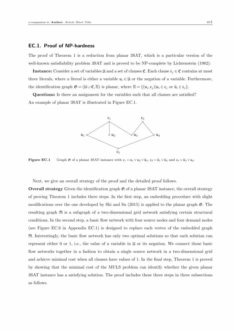
An example of planar 3SAT is illustrated in Figure EC.1.

u1 u2 u3 u4

c1

c2

c3

Figure EC.1 Graph G of a planar 3SAT instance with c1 = u1 ∨ u2 ∨ u3, c2 = u1 ∨ u4 and c3 = u3 ∨ u4.

Next, we give an overall strategy of the proof and the detailed proof follows.

Overall strategy Given the identification graph G of a planar 3SAT instance, the overall strategy

of proving Theorem 1 includes three steps. In the first step, an embedding procedure with slight

modifications over the one developed by Shi and Su (2015) is applied to the planar graph G. The

resulting graph R is a subgraph of a two-dimensional grid network satisfying certain structural

conditions. In the second step, a basic flow network with four source nodes and four demand nodes

(see Figure EC.6 in Appendix EC.1) is designed to replace each vertex of the embedded graph

R. Interestingly, the basic flow network has only two optimal solutions so that each solution can

represent either 0 or 1, i.e., the value of a variable in U or its negation. We connect those basic

flow networks together in a fashion to obtain a single source network in a two-dimensional grid

and achieve minimal cost when all clauses have values of 1. In the final step, Theorem 1 is proved

by showing that the minimal cost of the MULS problem can identify whether the given planar

3SAT instance has a satisfying solution. The proof includes these three steps in three subsections

as follows.

ec2 e-companion to Author: Article Short Title

EC.1.1. Embedding

Given the identification graph G of an instance of planar 3SAT, we follow the procedure used by

Shi and Su (2015) to embed it into a rectilinear grid and denote the embedded graph as R. We

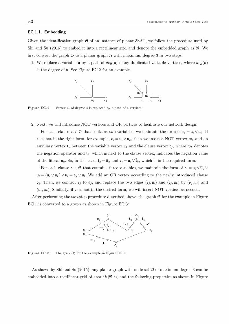
first convert the graph G to a planar graph H with maximum degree 3 in two steps:

1. We replace a variable u by a path of deg(u) many duplicated variable vertices, where deg(u)

is the degree of u. See Figure EC.2 for an example.

uic1

c2 c3

c4 ui

uiui

uic1

c2 c3

c4

Figure EC.2 Vertex ui of degree 4 is replaced by a path of 4 vertices.

2. Next, we will introduce NOT vertices and OR vertices to facilitate our network design.

For each clause cj ∈G that contains two variables, we maintain the form of cj = ui ∨ uk. If

cj is not in the right form, for example, cj = ui ∨ uk, then we insert a NOT vertex wk and an

auxiliary vertex tk between the variable vertex uk and the clause vertex cj, where wk denotes

the negation operator and tk, which is next to the clause vertex, indicates the negation value

of the literal uk. So, in this case, tk = uk and cj = ui ∨ tk, which is in the required form.

For each clause cj ∈G that contains three variables, we maintain the form of cj = ui ∨ uk ∨

ul = (ui ∨ uk) ∨ ul = oj ∨ ul. We add an OR vertex according to the newly introduced clause

oj. Then, we connect cj to oj, and replace the two edges (cj,ui) and (cj,uk) by (oj,ui) and

(oj,uk). Similarly, if cj is not in the desired form, we will insert NOT vertices as needed.

After performing the two-step procedure described above, the graph G for the example in Figure

EC.1 is converted to a graph as shown in Figure EC.3:

u1u1

u2 u3 u4

c1

c2

c3

w3

t3w4

t4o1

w2

t2

w1t1

Figure EC.3 The graph H for the example in Figure EC.1.

As shown by Shi and Su (2015), any planar graph with node set V of maximum degree 3 can be

embedded into a rectilinear grid of area O(|V|2), and the following properties as shown in Figure

e-companion to Author: Article Short Title ec3

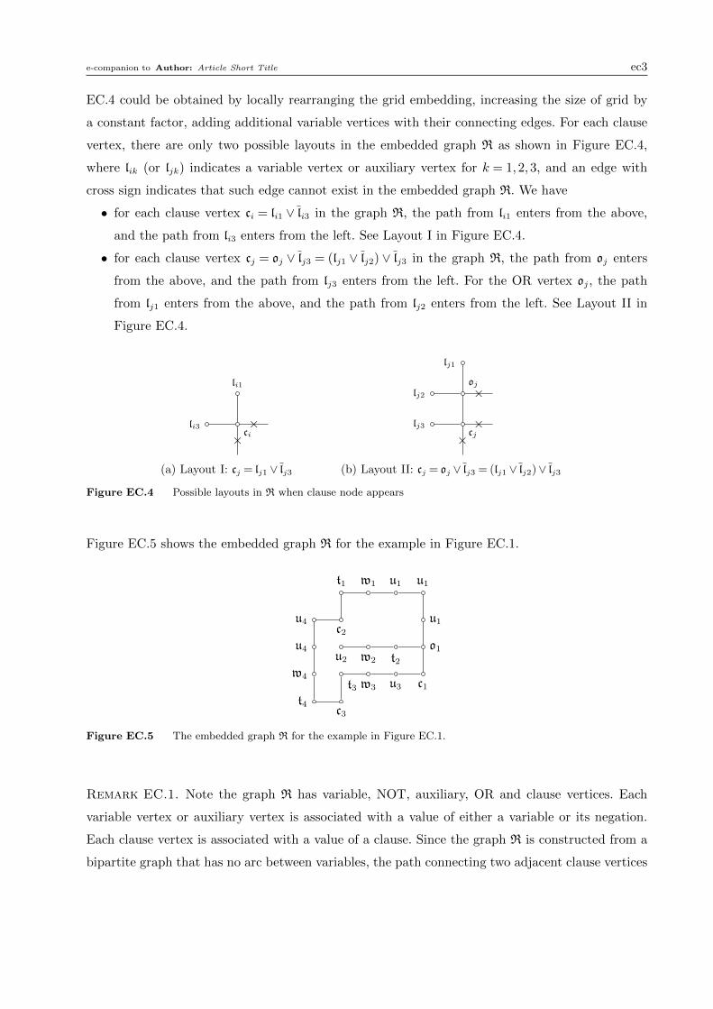
EC.4 could be obtained by locally rearranging the grid embedding, increasing the size of grid by

a constant factor, adding additional variable vertices with their connecting edges. For each clause

vertex, there are only two possible layouts in the embedded graph R as shown in Figure EC.4,

where lik (or ljk) indicates a variable vertex or auxiliary vertex for k = 1,2,3, and an edge with

cross sign indicates that such edge cannot exist in the embedded graph R. We have

• for each clause vertex ci = li1 ∨ li3 in the graph R, the path from li1 enters from the above,

and the path from li3 enters from the left. See Layout I in Figure EC.4.

• for each clause vertex cj = oj ∨ lj3 = (lj1 ∨ lj2) ∨ lj3 in the graph R, the path from oj enters

from the above, and the path from lj3 enters from the left. For the OR vertex oj, the path

from lj1 enters from the above, and the path from lj2 enters from the left. See Layout II in

Figure EC.4.

li3ci

li1

××

(a) Layout I: cj = lj1 ∨ lj3

lj3

lj2

lj1

cj

oj

××

×

(b) Layout II: cj = oj ∨ lj3 = (lj1 ∨ lj2)∨ lj3

Figure EC.4 Possible layouts in R when clause node appears

Figure EC.5 shows the embedded graph R for the example in Figure EC.1.

t4c3

w4t3 w3 u3 c1

u4

u4c2

t1 w1 u1 u1

u1

o1u2 w2 t2

Figure EC.5 The embedded graph R for the example in Figure EC.1.

Remark EC.1. Note the graph R has variable, NOT, auxiliary, OR and clause vertices. Each

variable vertex or auxiliary vertex is associated with a value of either a variable or its negation.

Each clause vertex is associated with a value of a clause. Since the graph R is constructed from a

bipartite graph that has no arc between variables, the path connecting two adjacent clause vertices

ec4 e-companion to Author: Article Short Title

is composed of vertices derived only from the same variable. For example, the path could consist

of vertices ui, wi or ti as they are all derived form the same variable ui ∈ U. Based on our way

of adding NOT and auxiliary vertices, the OR and clause vertices do not directly connect to any

NOT vertices.

EC.1.2. Flow network design

It is well-known that multiechelon lot-sizing problem can be modeled as a single source network

flow problem in a two-dimensional grid, see Zangwill (1969). In this section, we use a basic network

in Figure EC.6 to replace variable and auxiliary vertices in the embedded graph R. With careful

design on the connections, we can show that the satisfiability problem on R is related to a MULS

problem. Throughout this subsection, we make the following conventions in our flow network design:

• The arcs that are not shown in the network design have high fixed costs or inventory holding

costs. Thus, they are prohibited in the minimal cost flow,

• The dotted arcs are free, i.e. no cost is associated with them,

• The demand nodes are white dots in each figure with 1 unit demand,

• Vertical arcs connect the same time periods between different echelons. The fixed costs are

shown in each figure and the production costs are always 0,

• Horizontal arcs connect periods in the same echelon. Most of the inventory holding costs are

0. The nonzero inventory holding cost occurs only in one period right before each demand

node (with one exception in Figure EC.9b which will be elaborated later) and the value is

pointed out by an arrow in figures.

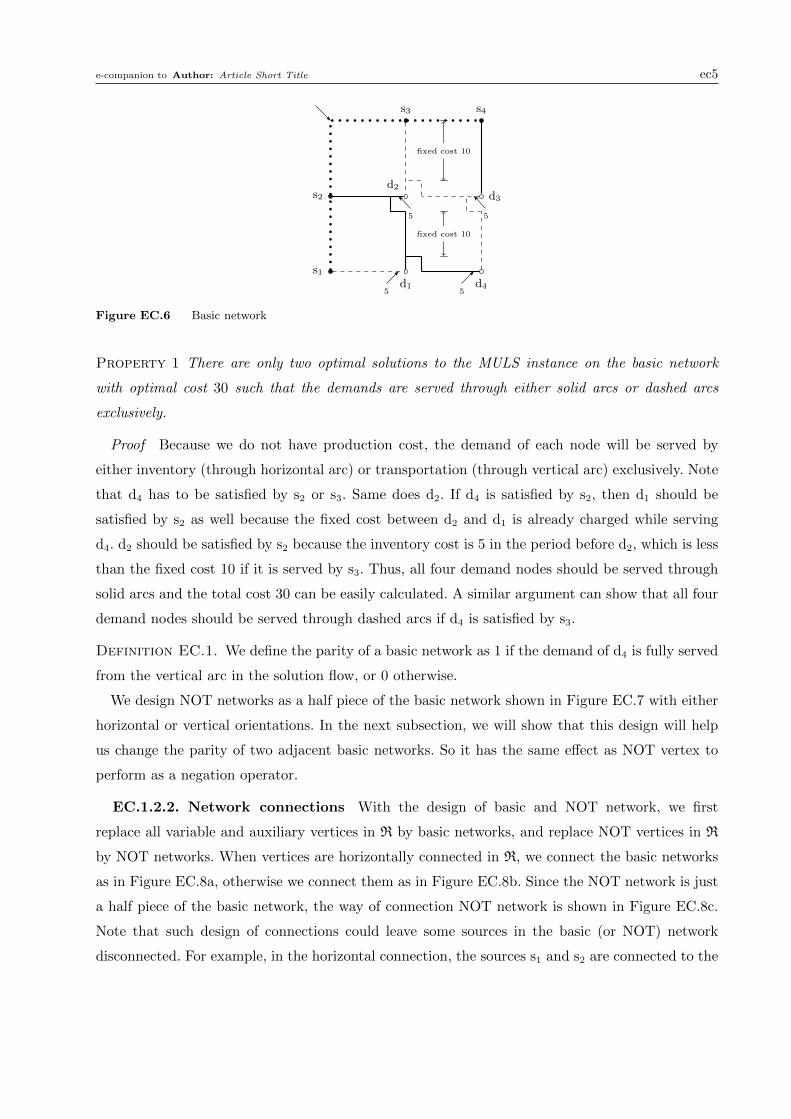
EC.1.2.1. Basic network The basic network is designed as in Figure EC.6 and it is the

most important building block. This simple network has four potential sources s1, . . . , s4 and four

demand nodes d1, . . . ,d4. The inventory holding cost is 5 in one period before each demand node.

As shown in Figure EC.6, from the echelon of s3 to the echelon at one level higher than the echelon

of d2, we have fixed cost 10 for both dashed and solid vertical lines. Similar fixed cost structure

between nodes d2 and d1 (d3 and d4) is demonstrated in Figure EC.6. Note that the solid and

dashed lines are used in Figure EC.6 for the purpose of better illustration only, and they are not

crucial in our proof. The most important thing for a basic network is its parity which is defined

later in Definition EC.1.

If we connect all sources by free arcs (i.e. dotted arcs), the network turns out to have only one

single source, which is indicated by the arrow at the top–left corner. So, it is an MULS and we

have the following property

e-companion to Author: Article Short Title ec5

s1

s2

s3 s4

d1

d2

d3

d4

fixed cost 10

fixed cost 10

5

5

5

5

Figure EC.6 Basic network

Property 1 There are only two optimal solutions to the MULS instance on the basic network

with optimal cost 30 such that the demands are served through either solid arcs or dashed arcs

exclusively.

Proof Because we do not have production cost, the demand of each node will be served by

either inventory (through horizontal arc) or transportation (through vertical arc) exclusively. Note

that d4 has to be satisfied by s2 or s3. Same does d2. If d4 is satisfied by s2, then d1 should be

satisfied by s2 as well because the fixed cost between d2 and d1 is already charged while serving

d4. d2 should be satisfied by s2 because the inventory cost is 5 in the period before d2, which is less

than the fixed cost 10 if it is served by s3. Thus, all four demand nodes should be served through

solid arcs and the total cost 30 can be easily calculated. A similar argument can show that all four

demand nodes should be served through dashed arcs if d4 is satisfied by s3.

Definition EC.1. We define the parity of a basic network as 1 if the demand of d4 is fully served

from the vertical arc in the solution flow, or 0 otherwise.

We design NOT networks as a half piece of the basic network shown in Figure EC.7 with either

horizontal or vertical orientations. In the next subsection, we will show that this design will help

us change the parity of two adjacent basic networks. So it has the same effect as NOT vertex to

perform as a negation operator.

EC.1.2.2. Network connections With the design of basic and NOT network, we first

replace all variable and auxiliary vertices in R by basic networks, and replace NOT vertices in R

by NOT networks. When vertices are horizontally connected in R, we connect the basic networks

as in Figure EC.8a, otherwise we connect them as in Figure EC.8b. Since the NOT network is just

a half piece of the basic network, the way of connection NOT network is shown in Figure EC.8c.

Note that such design of connections could leave some sources in the basic (or NOT) network

disconnected. For example, in the horizontal connection, the sources s1 and s2 are connected to the

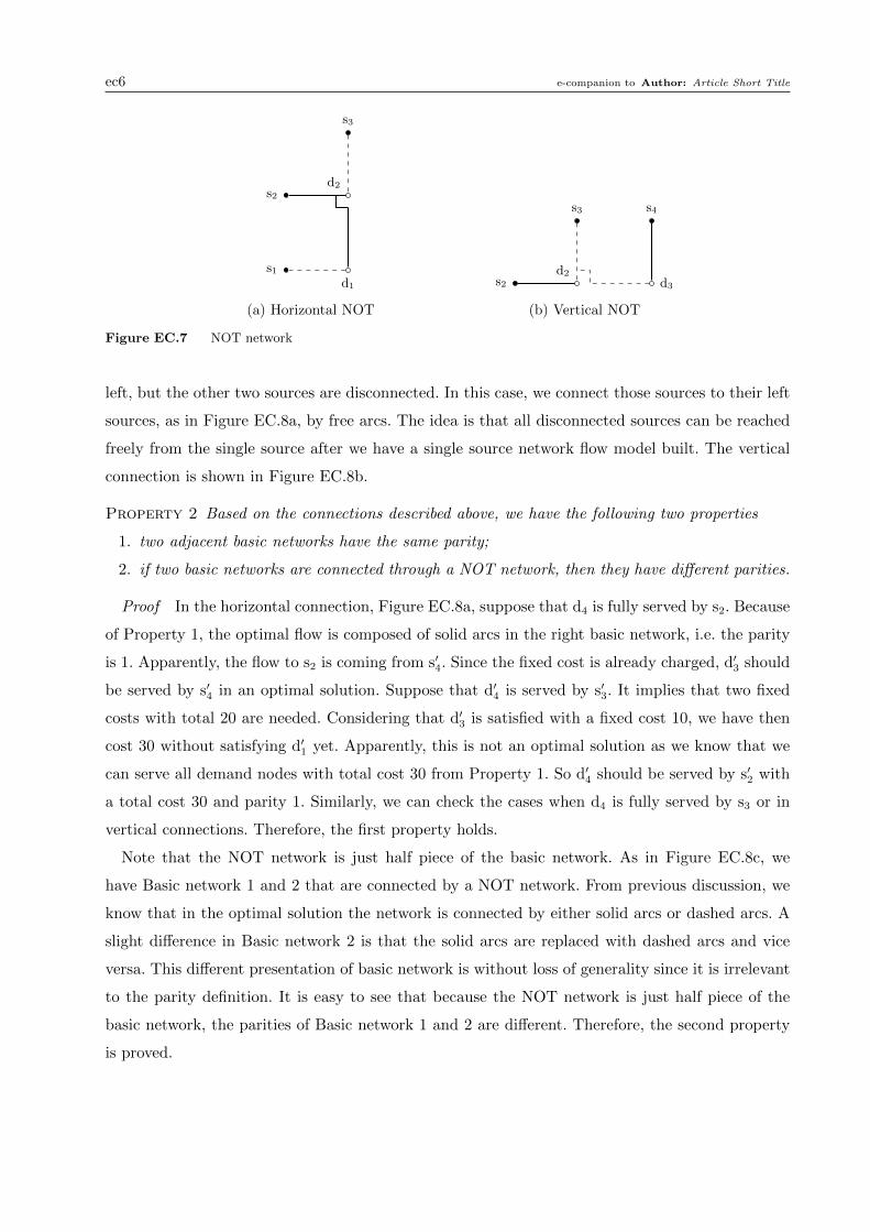
ec6 e-companion to Author: Article Short Title

s1

s2

s3

d1

d2

(a) Horizontal NOT

s2

s3 s4

d2

d3

(b) Vertical NOT

Figure EC.7 NOT network

left, but the other two sources are disconnected. In this case, we connect those sources to their left

sources, as in Figure EC.8a, by free arcs. The idea is that all disconnected sources can be reached

freely from the single source after we have a single source network flow model built. The vertical

connection is shown in Figure EC.8b.

Property 2 Based on the connections described above, we have the following two properties

1. two adjacent basic networks have the same parity;

2. if two basic networks are connected through a NOT network, then they have different parities.

Proof In the horizontal connection, Figure EC.8a, suppose that d4 is fully served by s2. Because

of Property 1, the optimal flow is composed of solid arcs in the right basic network, i.e. the parity

is 1. Apparently, the flow to s2 is coming from s′4. Since the fixed cost is already charged, d′3 should

be served by s′4 in an optimal solution. Suppose that d′4 is served by s′3. It implies that two fixed

costs with total 20 are needed. Considering that d′3 is satisfied with a fixed cost 10, we have then

cost 30 without satisfying d′1 yet. Apparently, this is not an optimal solution as we know that we

can serve all demand nodes with total cost 30 from Property 1. So d′4 should be served by s′2 with

a total cost 30 and parity 1. Similarly, we can check the cases when d4 is fully served by s3 or in

vertical connections. Therefore, the first property holds.

Note that the NOT network is just half piece of the basic network. As in Figure EC.8c, we

have Basic network 1 and 2 that are connected by a NOT network. From previous discussion, we

know that in the optimal solution the network is connected by either solid arcs or dashed arcs. A

slight difference in Basic network 2 is that the solid arcs are replaced with dashed arcs and vice

versa. This different presentation of basic network is without loss of generality since it is irrelevant

to the parity definition. It is easy to see that because the NOT network is just half piece of the

basic network, the parities of Basic network 1 and 2 are different. Therefore, the second property

is proved.

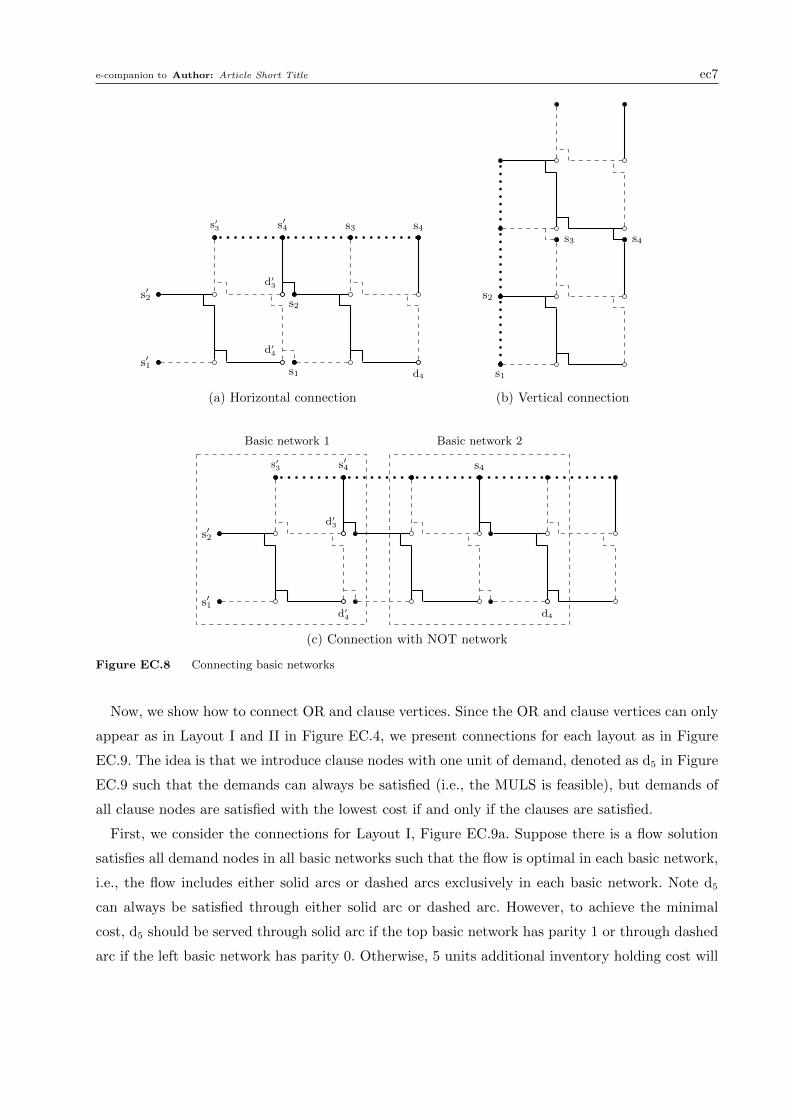
e-companion to Author: Article Short Title ec7

s2

s1

s3 s4s′4s′3

d′3

d′4

s′2

s′1d4

(a) Horizontal connection

s2

s1

s3 s4

(b) Vertical connection

s4s′4s′3

d′3

d′4

s′2

s′1d4

Basic network 1 Basic network 2

(c) Connection with NOT network

Figure EC.8 Connecting basic networks

Now, we show how to connect OR and clause vertices. Since the OR and clause vertices can only

appear as in Layout I and II in Figure EC.4, we present connections for each layout as in Figure

EC.9. The idea is that we introduce clause nodes with one unit of demand, denoted as d5 in Figure

EC.9 such that the demands can always be satisfied (i.e., the MULS is feasible), but demands of

all clause nodes are satisfied with the lowest cost if and only if the clauses are satisfied.

First, we consider the connections for Layout I, Figure EC.9a. Suppose there is a flow solution

satisfies all demand nodes in all basic networks such that the flow is optimal in each basic network,

i.e., the flow includes either solid arcs or dashed arcs exclusively in each basic network. Note d5

can always be satisfied through either solid arc or dashed arc. However, to achieve the minimal

cost, d5 should be served through solid arc if the top basic network has parity 1 or through dashed

arc if the left basic network has parity 0. Otherwise, 5 units additional inventory holding cost will

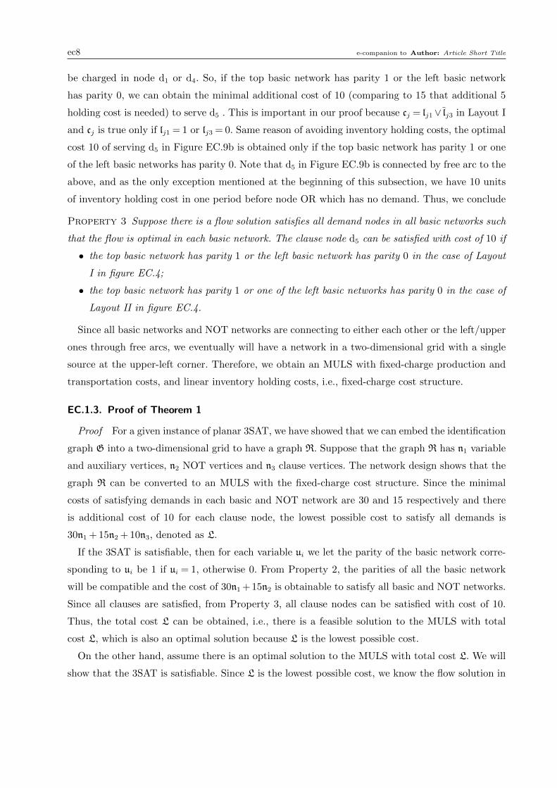
ec8 e-companion to Author: Article Short Title

be charged in node d1 or d4. So, if the top basic network has parity 1 or the left basic network

has parity 0, we can obtain the minimal additional cost of 10 (comparing to 15 that additional 5

holding cost is needed) to serve d5 . This is important in our proof because cj = lj1∨ lj3 in Layout I

and cj is true only if lj1 = 1 or lj3 = 0. Same reason of avoiding inventory holding costs, the optimal

cost 10 of serving d5 in Figure EC.9b is obtained only if the top basic network has parity 1 or one

of the left basic networks has parity 0. Note that d5 in Figure EC.9b is connected by free arc to the

above, and as the only exception mentioned at the beginning of this subsection, we have 10 units

of inventory holding cost in one period before node OR which has no demand. Thus, we conclude

Property 3 Suppose there is a flow solution satisfies all demand nodes in all basic networks such

that the flow is optimal in each basic network. The clause node d5 can be satisfied with cost of 10 if

• the top basic network has parity 1 or the left basic network has parity 0 in the case of Layout

I in figure EC.4;

• the top basic network has parity 1 or one of the left basic networks has parity 0 in the case of

Layout II in figure EC.4.

Since all basic networks and NOT networks are connecting to either each other or the left/upper

ones through free arcs, we eventually will have a network in a two-dimensional grid with a single

source at the upper-left corner. Therefore, we obtain an MULS with fixed-charge production and

transportation costs, and linear inventory holding costs, i.e., fixed-charge cost structure.

EC.1.3. Proof of Theorem 1

Proof For a given instance of planar 3SAT, we have showed that we can embed the identification

graph G into a two-dimensional grid to have a graph R. Suppose that the graph R has n1 variable

and auxiliary vertices, n2 NOT vertices and n3 clause vertices. The network design shows that the

graph R can be converted to an MULS with the fixed-charge cost structure. Since the minimal

costs of satisfying demands in each basic and NOT network are 30 and 15 respectively and there

is additional cost of 10 for each clause node, the lowest possible cost to satisfy all demands is

30n1 + 15n2 + 10n3, denoted as L.

If the 3SAT is satisfiable, then for each variable ui we let the parity of the basic network corre-

sponding to ui be 1 if ui = 1, otherwise 0. From Property 2, the parities of all the basic network

will be compatible and the cost of 30n1 +15n2 is obtainable to satisfy all basic and NOT networks.

Since all clauses are satisfied, from Property 3, all clause nodes can be satisfied with cost of 10.

Thus, the total cost L can be obtained, i.e., there is a feasible solution to the MULS with total

cost L, which is also an optimal solution because L is the lowest possible cost.

On the other hand, assume there is an optimal solution to the MULS with total cost L. We will

show that the 3SAT is satisfiable. Since L is the lowest possible cost, we know the flow solution in

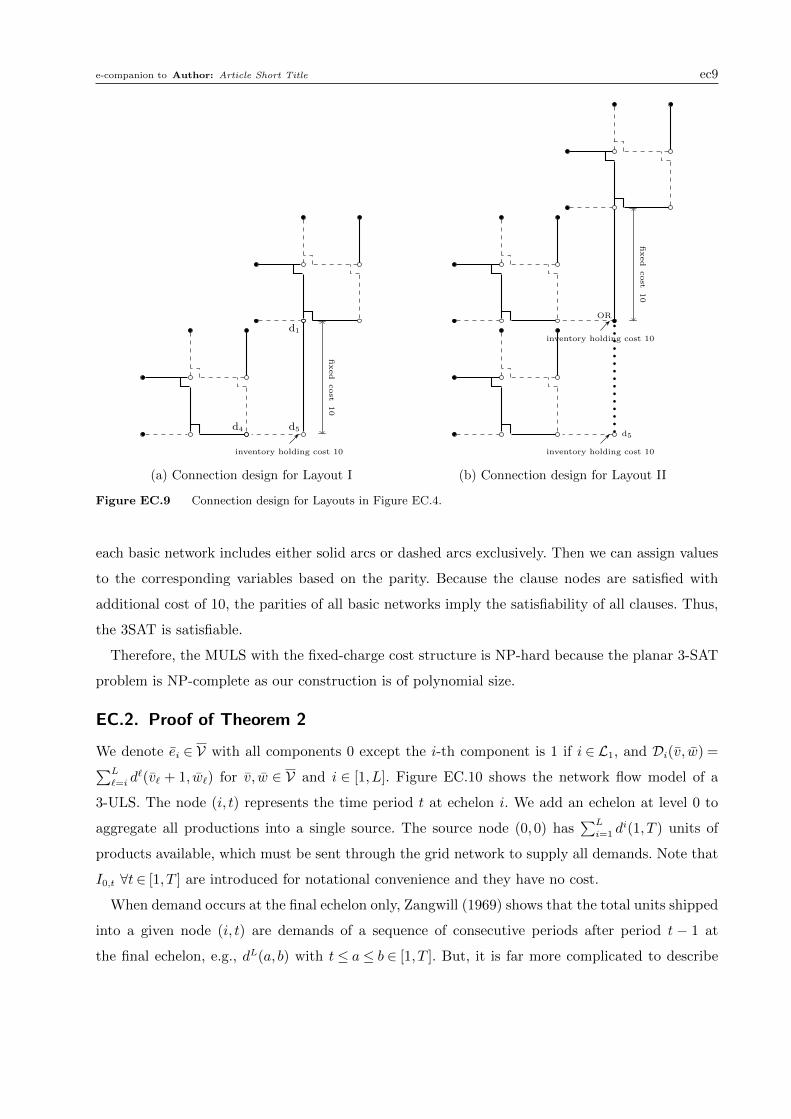
e-companion to Author: Article Short Title ec9

d5

d1

d4

inventory holding cost 10fi

xed

cost

10

(a) Connection design for Layout I

d5

OR

fixed

cost

10

inventory holding cost 10

inventory holding cost 10

(b) Connection design for Layout II

Figure EC.9 Connection design for Layouts in Figure EC.4.

each basic network includes either solid arcs or dashed arcs exclusively. Then we can assign values

to the corresponding variables based on the parity. Because the clause nodes are satisfied with

additional cost of 10, the parities of all basic networks imply the satisfiability of all clauses. Thus,

the 3SAT is satisfiable.

Therefore, the MULS with the fixed-charge cost structure is NP-hard because the planar 3-SAT

problem is NP-complete as our construction is of polynomial size.

EC.2. Proof of Theorem 2

We denote ei ∈ V with all components 0 except the i-th component is 1 if i ∈ L1, and Di(v, w) =∑L

`=i d`(v` + 1, w`) for v, w ∈ V and i ∈ [1,L]. Figure EC.10 shows the network flow model of a

3-ULS. The node (i, t) represents the time period t at echelon i. We add an echelon at level 0 to

aggregate all productions into a single source. The source node (0,0) has∑L

i=1 di(1, T ) units of

products available, which must be sent through the grid network to supply all demands. Note that

I0,t ∀t∈ [1, T ] are introduced for notational convenience and they have no cost.

When demand occurs at the final echelon only, Zangwill (1969) shows that the total units shipped

into a given node (i, t) are demands of a sequence of consecutive periods after period t − 1 at

the final echelon, e.g., dL(a, b) with t≤ a≤ b ∈ [1, T ]. But, it is far more complicated to describe

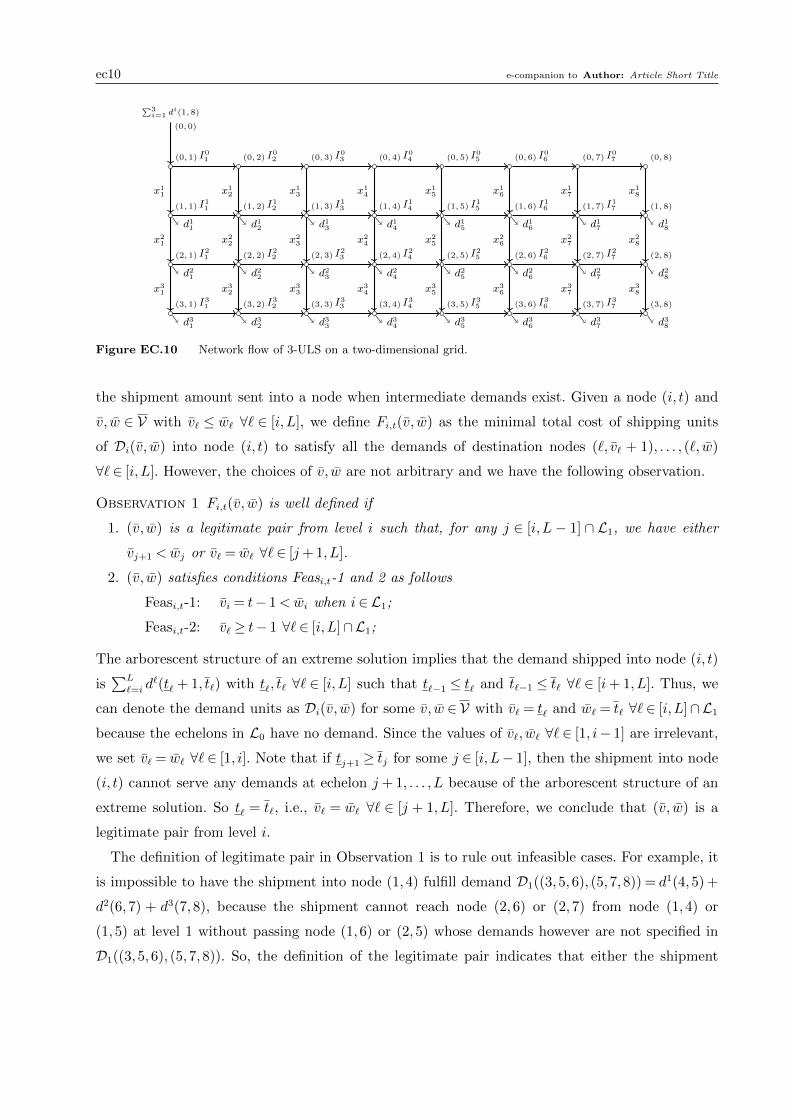
ec10 e-companion to Author: Article Short Title

(0,1)

(1,1)

(0,2) (0,3) (0,4) (0,5) (0,6) (0,7) (0,8)

(2,1)

(1,2) (1,3) (1,4) (1,5) (1,6) (1,7) (1,8)

(3,1)

(2,2) (2,3) (2,4) (2,5) (2,6) (2,7) (2,8)

(3,2) (3,3) (3,4) (3,5) (3,6) (3,7) (3,8)

∑3i=1 d

i(1,8)

(0,0)

x11

I01

x12

I02

x13

I03

x14

I04

x15

I05

x16

I06

x17

I07

x18

d11

x21

I11

d12

x22

I12

d13

x23

I13

d14

x24

I14

d15

x25

I15

d16

x26

I16

d17

x27

I17

d18

x28

d21

x31

I21

d22

x32

I22

d23

x33

I23

d24

x34

I24

d25

x35

I25

d26

x36

I26

d27

x37

I27

d28

x38

d31

I31

d32

I32

d33

I33

d34

I34

d35

I35

d36

I36

d37

I37

d38

Figure EC.10 Network flow of 3-ULS on a two-dimensional grid.

the shipment amount sent into a node when intermediate demands exist. Given a node (i, t) and

v, w ∈ V with v` ≤ w` ∀` ∈ [i,L], we define Fi,t(v, w) as the minimal total cost of shipping units

of Di(v, w) into node (i, t) to satisfy all the demands of destination nodes (`, v` + 1), . . . , (`, w)

∀`∈ [i,L]. However, the choices of v, w are not arbitrary and we have the following observation.

Observation 1 Fi,t(v, w) is well defined if

1. (v, w) is a legitimate pair from level i such that, for any j ∈ [i,L− 1] ∩ L1, we have either

vj+1 < wj or v` = w` ∀`∈ [j+ 1,L].

2. (v, w) satisfies conditions Feasi,t-1 and 2 as follows

Feasi,t-1: vi = t− 1< wi when i∈L1;

Feasi,t-2: v` ≥ t− 1 ∀`∈ [i,L]∩L1;

The arborescent structure of an extreme solution implies that the demand shipped into node (i, t)

is∑L

`=i d`(t` + 1, t`) with t`, t` ∀` ∈ [i,L] such that t`−1 ≤ t` and t`−1 ≤ t` ∀` ∈ [i+ 1,L]. Thus, we

can denote the demand units as Di(v, w) for some v, w ∈ V with v` = t` and w` = t` ∀`∈ [i,L]∩L1

because the echelons in L0 have no demand. Since the values of v`, w` ∀`∈ [1, i− 1] are irrelevant,

we set v` = w` ∀` ∈ [1, i]. Note that if tj+1 ≥ tj for some j ∈ [i,L− 1], then the shipment into node

(i, t) cannot serve any demands at echelon j + 1, . . . ,L because of the arborescent structure of an

extreme solution. So t` = t`, i.e., v` = w` ∀` ∈ [j + 1,L]. Therefore, we conclude that (v, w) is a

legitimate pair from level i.

The definition of legitimate pair in Observation 1 is to rule out infeasible cases. For example, it

is impossible to have the shipment into node (1,4) fulfill demand D1((3,5,6), (5,7,8)) = d1(4,5) +

d2(6,7) + d3(7,8), because the shipment cannot reach node (2,6) or (2,7) from node (1,4) or

(1,5) at level 1 without passing node (1,6) or (2,5) whose demands however are not specified in

D1((3,5,6), (5,7,8)). So, the definition of the legitimate pair indicates that either the shipment

e-companion to Author: Article Short Title ec11

reaches level j + 1 (i.e., vj+1 < wj) or stops at level j (i.e., v` = w` ∀` ∈ [j + 1,L]). Note that if

(v, w) is a legitimate pair from level i, then we have (v, w) as a legitimate pair from level i+ 1 and

(v+ ei, w) as a legitimate pair from level i by the definition.

In addition, the condition Feasi,t-1 in Observation 1 is needed because the demand of node (i, t)

has to be satisfied by the shipment into node (i, t) if i∈L1. The condition Feasi,t-2 states that the

shipment into node (i, t) can only cover demands in or after period t.

Our goal is to determine the value of F0,1(0,T), which is well defined by easily checking the

conditions in Observation 1. Now, with a given node (i, t), it is important to note that the units

shipped into node (i, t) will be fully distributed to nodes (i + 1, t) and (i, t + 1). In the rest of

this subsection, we suppose that Fi,t(v, w) is well defined with a given node (i, t) and v, w ∈ V,

v` ≤ w` ∀` ∈ [i,L]. Without loss of generality, we assume v` ≥ t if v` = w` with some ` ∈ [i,L]∩L1

for notational convenience. It is easy to see that there is no change on the definition of Fi,t(v, w)

because v` = w` implies [v`+ 1, w] = ∅. Let Ωi,t(v, w) be the set of u∈ V such that u` = v` ∀`∈ [1, i],

max(t, v`)≤ u` ≤ w` ∀` ∈ [i+ 1,L] ∩L1, (v, u) is a legitimate pair from level i+ 1 and (u, w) is a

legitimate pair from level i. We point out that Ωi,t(v, w) 6= ∅ because we can set u` = v` ∀`∈ [1, i] and

u` = w` ∀`∈ [i+ 1,L]. The purpose of having the set Ωi,t(v, w) is to make sure that the shipments

from node (i, t) to nodes (i + 1, t) and (i, t + 1) can be denoted as Di+1(v, u) and Di(u + ei, w)

respectively. By introducing two conditions (C1)-(C2),

(C1): vi+1 ≥ t and i+ 1∈L1;

(C2): vi + 1 = wi and i∈L1.

we can generalize one of the main theorems by Zangwill (1969) as in Proposition EC.1. The

conditions (C1) and (C2) identify the cases that the shipment sending out from node (i, t) is sent to

only one node (i+ 1, t) or (i, t+ 1), which gives boundary conditions of the dynamic programming

recursions.

Proposition EC.1. The shipment pattern of an extreme solution from node (i, t) can be charac-

terized into four cases.

1. If conditions (C1) and (C2) do not hold, and i < L, t < T , then there exists a vector u ∈Ωi,t(v, w) such that the amount shipped into node (i, t) is sent to node (i+ 1, t) and (i, t+ 1)

with amount Di+1(v, u) and Di(u+ ei, w) respectively and

xi+1t =Di+1(v, u) and I it =Di(u+ ei, w).

In this case, we have the dynamic programming recursion

Fi,t(v, w) = minu∈Ωi,t(v,w)

[pi+1t (Di(v, u)) +Fi+1,t(v, u) +hit(Di(u+ ei, w)) +Fi,t+1(u+ ei, w)

],

(EC.1)

with Fi+1,t(v, u) and Fi,t+1(u+ ei, w) to be well defined.

ec12 e-companion to Author: Article Short Title

2. if condition (C1) holds or i=L, then the amount shipped into node (i, t) is fully sent to node

(i, t+ 1) with I it =Di(v+ ei, w). In this case, we have the boundary condition

Fi,t(v, w) = hit(Di(v+ ei, w)) +Fi,t+1(v+ ei, w),

with Fi,t+1(v+ ei, w) to be well defined.

3. if condition (C2) holds or t= T , then the amount shipped into node (i, t) is fully sent to node

(i+ 1, t) with xi+1t =Di(v, w) if i < L. In this case, we have the boundary condition

Fi,t(v, w) = pi+1t (Di(v, w)) +Fi+1,t(v, w),

with Fi+1,t(v, w) to be well defined.

4. if condition (C1)-(C2) hold or (i, t) = (L,T ), then there is no shipment to be sent out from

node (i, t). In this case, we have Fi,t(v, w) = 0.

Note that the vector ei in defining I it indicates that the demand dit is consumed at node (i, t).

Proof Let us consider the first case where i < L, t < T . It is well known that the flow corre-

sponding to any extreme solution is acyclic (see, e.g., Ahuja et al. (1993)) in uncapacitated network

flow problems. Thus, the total shipment Di(v, w) into node (i, t) will be sent to nodes (i+ 1, t) and

(i, t+ 1), with amount∑L

`=i+1 d`(v` + 1, u`) and di(t+ 1, wi) +

∑L

`=i+1 d`(u` + 1, w`) respectively.

Since u` ∀` ≤ i are not involved in the description, we can set u` = v` ∀` ≤ i for the convenience

of recursions. Because of the arborescent structure of an extreme solution, we know v` ≤ u` ≤ w`∀` ∈ [i+ 1,L]∩L1. As the same reason of introducing Observation 1, we will discuss a few more

properties about u`s because they are used to describe the amount shipped into nodes (i+ 1, t)

and (i, t+ 1) and cannot be arbitrary. First, we need (v, u) to be legitimate from level i+ 1 and

(u, w) to be legitimate from level i. Next, because the shipment di(t+ 1, wi) +∑L

`=i+1 d`(u`+ 1, w`)

into node (i, t+ 1) only covers demands after period t, we have u` ≥ t for all `∈ [i+ 1,L]∩L1. By

summarizing the above discussions, we conclude that u ∈ V, u ∈ Ωi,t(v, w) and the shipment sent

to node (i+ 1, t) (i.e., xi+1t ) and (i, t+ 1) (i.e., I it) can be written as Di+1(v, u) and Di(u+ ei, w)

respectively. The vector ei is used to indicate that the demand dit is consumed at node (i, t). Note

that di(t+ 1, wi) = di(ui + ei, wi) because the condition Feasi,t-1 implies ui = vi = t− 1 if i∈L1. It

also implies that u+ ei ∈ V as ui = vi = t− 1≤ t≤ u` ∀`∈ [i+ 1,L]∩L1 if i∈L1.

With the shipping pattern, the recursion (EC.1) follows immediately by finding u with the

minimal total cost. Now, we need to show that Fi+1,t(v, u) and Fi,t+1(u+ ei, w) are well defined.

We consider Fi+1,t(v, u) first. We have already shown that (v, u) is legitimate from level i+1. Since

the condition (C1) does not hold, we have vi+1 = t− 1 if i+ 1 ∈ L1. Then u ∈ Ωi,t(v, w) implies

t ≤ ui+1 and vi+1 = t− 1 < t ≤ ui+1 if i+ 1 ∈ L1. The condition Feasi+1,t-1 holds for (v, u). The

e-companion to Author: Article Short Title ec13

condition Feasi+1,t-2 holds obviously for (v, u) because Feasi,t-2 holds for (v, w). Then, we consider

Fi,t+1(u+ ei, w). That (u, w) is legitimate from level i implies that (u+ ei, w) is legitimate from

level i by definition. Since the condition (C2) does not hold, we have vi + 1< wi if i ∈ L1. Then,

(u+ ei)i = ui + 1 = vi + 1 = t < wi if i ∈ L1. The condition Feasi,t+1-1 holds for (u+ ei, w). The

condition Feasi,t+1-2 holds obviously for (u+ ei, w) because u∈Ωi,t(v, w) and t≤ u` `∈ [i+1,L]∩L1.

Next, we consider the final case, i.e., the fourth case. It holds obviously if (i, t) = (L,T ). So,

we suppose that the conditions (C1) and (C2) hold. When the condition (C1) holds, the amount

shipped into node (i, t) is fully sent to node (i, t+1), because, if i+1∈L1, vi+1 ≥ t and the demand

of node (i+1, t) is not covered by the shipment into (i, t), i.e., no shipment sending from node (i, t)

to (i+ 1, t). When condition (C2) holds, the amount shipped into node (i, t) is fully sent to node

(i+ 1, t) because vi = t− 1 (since the condition Feasi,t-1 holds for (v, w)), t= vi + 1 = wi and the

demand of node (i, t+ 1) is not covered by the shipment into (i, t), i.e., no shipment sending from

node (i, t) to (i, t+ 1). Since there is no shipment sending out from node (i, t), we have boundary

condition Fi,t(v, w) = 0.

Finally, we show the second and third cases to conclude the proof. The second case holds obvi-

ously if i = L. As shown before, the condition (C1) implies that the amount shipped into node

(i, t) is fully sent to node (i, t+ 1). We only need to show that Fi,t+1(v+ ei, w) is well defined. Note

that (v+ ei, w) is legitimate from level i because (v, w) is legitimate from level i. We can assume

that condition (C2) does not hold, otherwise it becomes the last case, which will be shown later. It

implies that wi > vi+1 if i∈L1. Also that the condition Feasi,t-1 holds for (v, w) implies (v+ ei)` ≥ t

∀` ∈ [i,L] ∩ L1. Hence, (v + ei)i = vi + 1 = t < wi when i ∈ L1 and the condition Feasi,t+1-1 holds

for (v + ei, w). Since the condition (C1) holds, we have that i+ 1 ∈ L1 and (v + ei)i = t≤ vi+1 =

(v+ ei)i+1, which implies v+ ei ∈ V. Note that (v+ ei)` = v` ≥ vi+1 ≥ t= (v+ ei)i ∀`∈ [i+1,L]∩L1.

The condition Feasi,t+1-2 holds for (v+ ei, w).

The third case holds obviously if t = T . As shown before, the condition (C2) implies that the

amount shipped into node (i, t) is fully sent to node (i+1, t). We only need to show that Fi+1,t(v, w)

is well defined. By the definition, (v, w) is legitimate from level i+ 1 because (v, w) is legitimate

from level i. We can assume that condition (C1) does not hold, otherwise it becomes the last case,

which will be showed later. It implies that if i+ 1 ∈ L1, then vi+1 = t− 1. Because the condition

(C2) holds, wi+1 ≥ wi = vi + 1 = t > t− 1 = vi+1 if i+ 1 ∈ L1. The condition Feasi+1,t-1 holds for

(v, w). The condition Feasi+1,t-2 holds obviously for (v, w) because the condition Feasi,t-2 holds for

(v, w).

In Proposition EC.1, the application of the shipment pattern gives dynamic programming recur-

sions on Fi,t(v, w), which solve the MULS with concave cost functions. Apparently, the bottleneck

of the complexity is in recursion (EC.1) where we have O(T 3L1) choices of v, u, w as they are vectors

ec14 e-companion to Author: Article Short Title

in V and O(LT ) choices of indices i, t. With all these parameters are given, the recursion (EC.1)

can be evaluated in constant time. Therefore, Theorem 2 is proved.

EC.3. Proof of Theorem 3

Before presenting the proof, we highlight two properties. Because MULS with the fixed-charge cost

structure is a single source uncapacitated fixed-charge network flow problem, we can apply the well

known result that the extreme points of such problem correspond to a spanning tree (see Zangwill

(1968), Veinott (1969)) to conclude that

Property 4 (Zero Inventory Ordering (ZIO)) There exists an optimal basic feasible solution with

I it−1xit = 0 for all i∈ [1,L] and t∈ [1, T ].

The next property follows from the ZIO property.

Property 5 Suppose that I is = I it = 0 and the inventory quantities between time periods s+ 1 and

t at echelon i are all positive. Then, xis+1 = di(s+ 1, t) +∑t

τ=s+1 xi+1τ ∀i ∈ [1,L− 1] and xis+1 =

di(s+ 1, t) when i=L.

Proof From the inventory balance constraints (1b) and (1c), we get

I it =

t∑τ=1

(xiτ −xi+1τ )− di(1, t) ∀i∈ [1,L− 1]

t∑τ=1

xiτ − di(1, t) i=L

Thus, for all i∈ [1,L− 1],

0 = I is− I it =

(s∑

τ=1

(xiτ −xi+1τ )− di(1, s)

)−

(t∑

τ=1

(xiτ −xi+1τ )− di(1, t)

)

= xis+1− di(s+ 1, t)−t∑

τ=s+1

xi+1τ

Note that Property 4 implies xiτ = 0 for τ = s+ 2, . . . , t. Similarly, we can prove the case when

i=L.

Then, we are ready to prove Theorem 3.

Proof of Theorem 3 Given an extreme solution, the time horizon [0, T ] at each echelon i ∈

[1,L] is partitioned by regeneration intervals, which are composed of qi regeneration points 0 =

si1 < si2 < · · ·< siqi = T since the starting and ending inventory quantities are 0 by the problem

definition. Thus, the total demand can be partitioned by demands on regeneration intervals and

e-companion to Author: Article Short Title ec15

Property 5 implies that the demands on each regeneration interval are fulfilled by one production

or transportation. For example, for echelon i and k ∈ [1, qi], Property 5 implies

xisik+1 = di(sik + 1, si,k+1) +

si,k+1∑τ=sik+1

xi+1τ , (EC.2)

i.e., the demands di(sik + 1, si,k+1) are satisfied by xisik+1. To realize the demands di(sik + 1, si,k+1)

and the associated cost in a path in G, we have two regeneration vectors v,w such that vi = sik and

wi = si,k+1. For other components of v,w, we have v` =w` ∀`∈ [1,L]\i and they can be obtained

iteratively as follows. First, if i > 1, then we have an index j such that si−1,j ≤ sik < si−1,j+1 and we

set vi−1 = wi−1 = si−1,j. The index j is unique because the regeneration intervals at each echelon

give partitions of [0, T ]. Applying Property 5 on echelon i− 1 and periods si−1,j, si−1,j+1, we have

xi−1si−1,j+1 = di−1(si−1,j + 1, si−1,j+1) +

si−1,j+1∑τ=si−1,j+1

xiτ . (EC.3)

Because si−1,j ≤ sik < si−1,j+1, the choice of vi−1(= si−1,j) indicates that the shipment quantity

xivi+1(= xisik+1) is fulfilled by the production or shipment quantity xi−1vi−1+1(= xi−1

si−1,j+1). Thus, we

need to count the shipment cost di(vi + 1,wi)ci−1vi−1+1 for the demand di(vi + 1,wi). This procedure

can be applied iteratively to all echelons 1, . . . , i− 1 and the total cost is

di(vi + 1,wi)i−1∑`=1

c`v`+1 + di(vi + 1,wi)civi+1 + f ivi

where the first term is the aggregated production and transportation costs from all echelons

1, . . . , i−1, the second term is the transportation cost at echelon i and f ivi is the fixed cost if xisik+1

is positive. Next, if i < L, then we have a unique index r (the uniqueness follows a similar rea-

soning as above) such that si+1,r−1 < si,k+1 ≤ si+1,r and we set vi+1 =wi+1 = si+1,r. From equation

(EC.2) and si+1,r−1 < si,k+1 ≤ si+1,r, we know the quantity xi+1si+1,r−1+1 is coming from xisik+1 and

xi+1si+1,r+1 is not. Thus, the choice of vi+1 indicates that the transportation quantities xi+1

1 , . . . , xi+1vi+1

and demands di+1(1, si+1,r) are fulfilled by the production and transportation quantities xi1, . . . , xivi

.

Again, iteratively applying the procedure to all the lower echelons of i, we have regeneration vectors

v,w built and know that the production and transportation quantities xi1, . . . , xivi

have satisfied

demands∑L

`=i+1 d`(1, v`), i.e., when we build the path recursively, the demands

∑L

`=i+1 d`(1, v`)

have already been fulfilled.

Now, we show that the fixed cost defined in the arc cost is valid. Note that if xivi+1 = xisik+1 > 0,

then di(vi + 1,wi) +∑L

`=i+1 d`(1, v`)> 0 obviously. So the fixed cost f ivi will be definitely included

into arc cost of (v,w) if it is necessary. We need to check if the fixed cost defined in the arc cost

is valid when xisik+1 = 0 but di(vi + 1,wi) +∑L

`=i+1 d`(1, v`) 6= 0. Apparently, in such case, the fixed

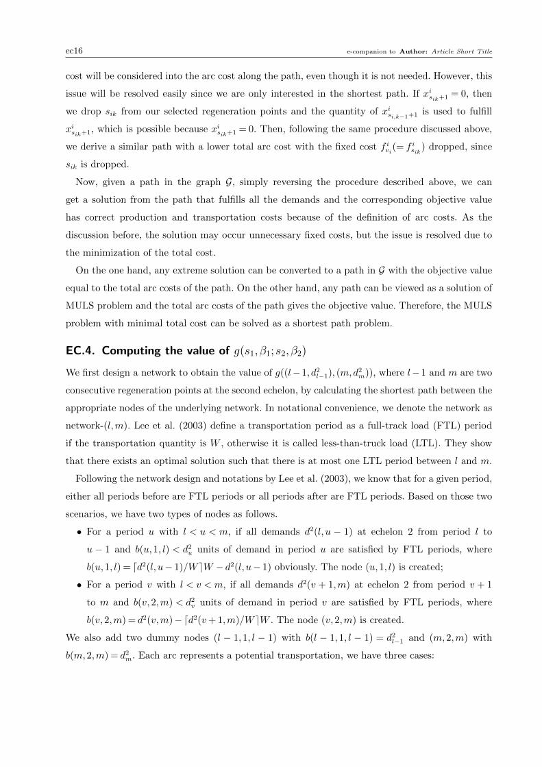
ec16 e-companion to Author: Article Short Title

cost will be considered into the arc cost along the path, even though it is not needed. However, this

issue will be resolved easily since we are only interested in the shortest path. If xisik+1 = 0, then

we drop sik from our selected regeneration points and the quantity of xisi,k−1+1 is used to fulfill

xisik+1, which is possible because xisik+1 = 0. Then, following the same procedure discussed above,

we derive a similar path with a lower total arc cost with the fixed cost f ivi(= f isik) dropped, since

sik is dropped.

Now, given a path in the graph G, simply reversing the procedure described above, we can

get a solution from the path that fulfills all the demands and the corresponding objective value

has correct production and transportation costs because of the definition of arc costs. As the

discussion before, the solution may occur unnecessary fixed costs, but the issue is resolved due to

the minimization of the total cost.

On the one hand, any extreme solution can be converted to a path in G with the objective value

equal to the total arc costs of the path. On the other hand, any path can be viewed as a solution of

MULS problem and the total arc costs of the path gives the objective value. Therefore, the MULS

problem with minimal total cost can be solved as a shortest path problem.

EC.4. Computing the value of g(s1, β1;s2, β2)

We first design a network to obtain the value of g((l−1, d2l−1), (m,d2

m)), where l−1 and m are two

consecutive regeneration points at the second echelon, by calculating the shortest path between the

appropriate nodes of the underlying network. In notational convenience, we denote the network as

network-(l,m). Lee et al. (2003) define a transportation period as a full-track load (FTL) period

if the transportation quantity is W , otherwise it is called less-than-truck load (LTL). They show

that there exists an optimal solution such that there is at most one LTL period between l and m.

Following the network design and notations by Lee et al. (2003), we know that for a given period,

either all periods before are FTL periods or all periods after are FTL periods. Based on those two

scenarios, we have two types of nodes as follows.

• For a period u with l < u < m, if all demands d2(l, u − 1) at echelon 2 from period l to

u − 1 and b(u,1, l) < d2u units of demand in period u are satisfied by FTL periods, where

b(u,1, l) = dd2(l, u− 1)/W eW − d2(l, u− 1) obviously. The node (u,1, l) is created;

• For a period v with l < v < m, if all demands d2(v + 1,m) at echelon 2 from period v + 1

to m and b(v,2,m) < d2v units of demand in period v are satisfied by FTL periods, where

b(v,2,m) = d2(v,m)−dd2(v+ 1,m)/W eW . The node (v,2,m) is created.

We also add two dummy nodes (l − 1,1, l − 1) with b(l − 1,1, l − 1) = d2l−1 and (m,2,m) with

b(m,2,m) = d2m. Each arc represents a potential transportation, we have three cases:

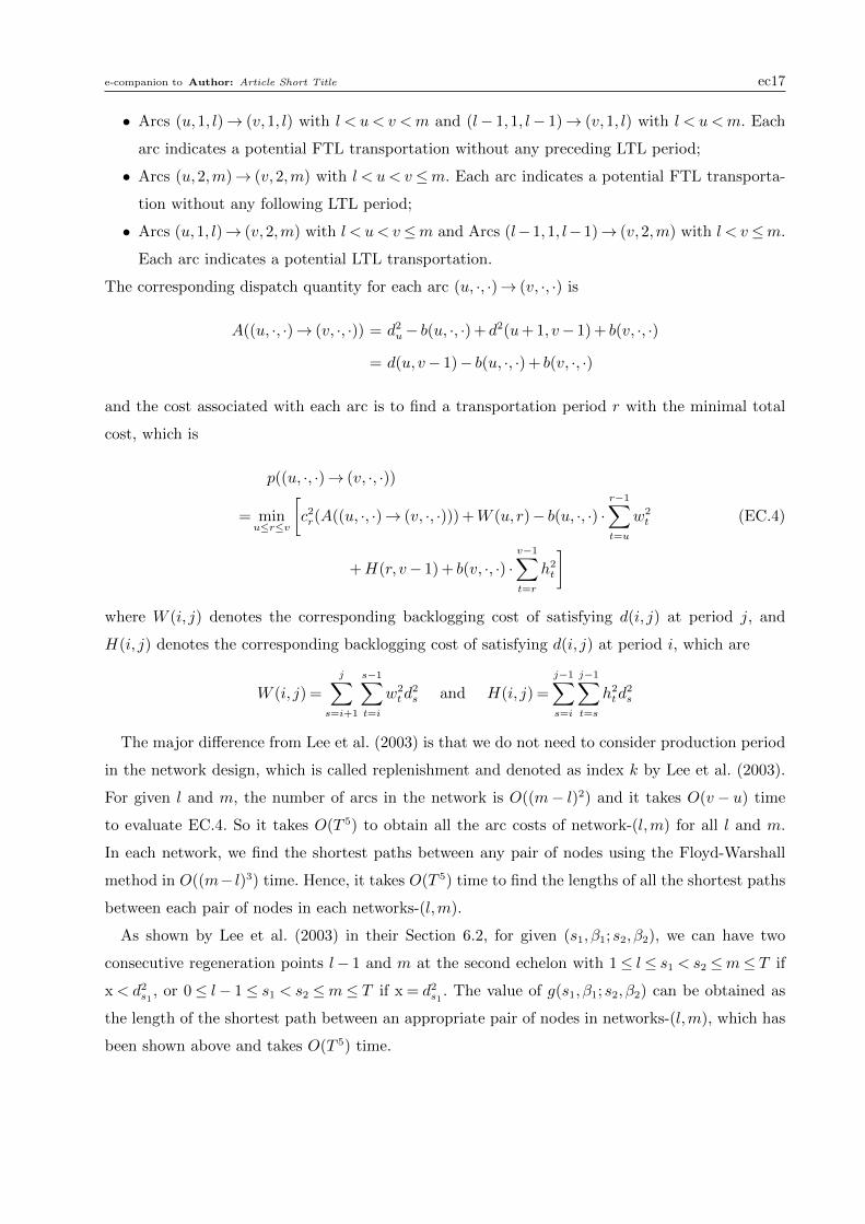
e-companion to Author: Article Short Title ec17

• Arcs (u,1, l)→ (v,1, l) with l < u < v <m and (l− 1,1, l− 1)→ (v,1, l) with l < u <m. Each

arc indicates a potential FTL transportation without any preceding LTL period;

• Arcs (u,2,m)→ (v,2,m) with l < u < v ≤m. Each arc indicates a potential FTL transporta-

tion without any following LTL period;

• Arcs (u,1, l)→ (v,2,m) with l < u< v≤m and Arcs (l−1,1, l−1)→ (v,2,m) with l < v≤m.

Each arc indicates a potential LTL transportation.

The corresponding dispatch quantity for each arc (u, ·, ·)→ (v, ·, ·) is

A((u, ·, ·)→ (v, ·, ·)) = d2u− b(u, ·, ·) + d2(u+ 1, v− 1) + b(v, ·, ·)

= d(u, v− 1)− b(u, ·, ·) + b(v, ·, ·)

and the cost associated with each arc is to find a transportation period r with the minimal total

cost, which is

p((u, ·, ·)→ (v, ·, ·))

= minu≤r≤v

[c2r(A((u, ·, ·)→ (v, ·, ·))) +W (u, r)− b(u, ·, ·) ·

r−1∑t=u

w2t (EC.4)

+H(r, v− 1) + b(v, ·, ·) ·v−1∑t=r

h2t

]where W (i, j) denotes the corresponding backlogging cost of satisfying d(i, j) at period j, and

H(i, j) denotes the corresponding backlogging cost of satisfying d(i, j) at period i, which are

W (i, j) =

j∑s=i+1

s−1∑t=i

w2t d

2s and H(i, j) =

j−1∑s=i

j−1∑t=s

h2td

2s

The major difference from Lee et al. (2003) is that we do not need to consider production period

in the network design, which is called replenishment and denoted as index k by Lee et al. (2003).

For given l and m, the number of arcs in the network is O((m− l)2) and it takes O(v − u) time

to evaluate EC.4. So it takes O(T 5) to obtain all the arc costs of network-(l,m) for all l and m.

In each network, we find the shortest paths between any pair of nodes using the Floyd-Warshall

method in O((m− l)3) time. Hence, it takes O(T 5) time to find the lengths of all the shortest paths

between each pair of nodes in each networks-(l,m).

As shown by Lee et al. (2003) in their Section 6.2, for given (s1, β1;s2, β2), we can have two

consecutive regeneration points l− 1 and m at the second echelon with 1≤ l≤ s1 < s2 ≤m≤ T if

x< d2s1

, or 0≤ l− 1≤ s1 < s2 ≤m≤ T if x = d2s1

. The value of g(s1, β1;s2, β2) can be obtained as

the length of the shortest path between an appropriate pair of nodes in networks-(l,m), which has

been shown above and takes O(T 5) time.

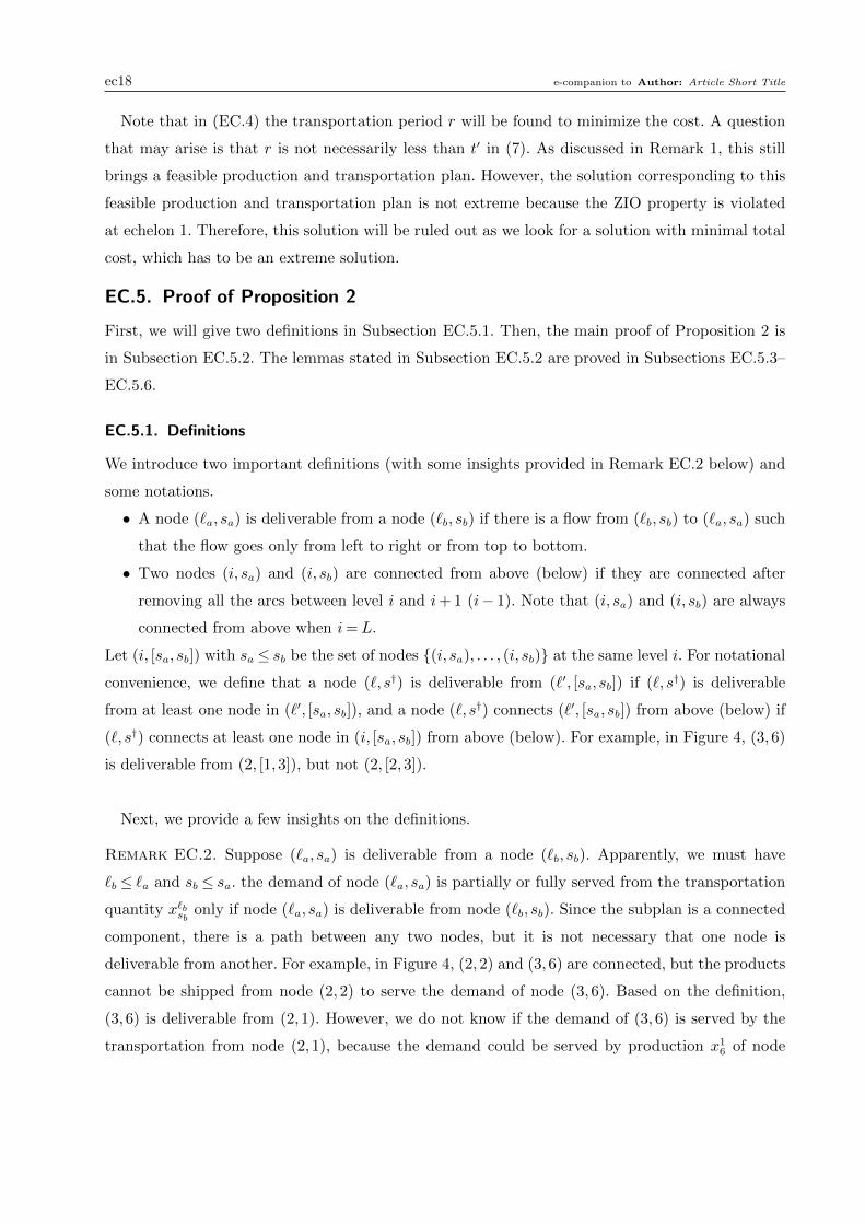
ec18 e-companion to Author: Article Short Title

Note that in (EC.4) the transportation period r will be found to minimize the cost. A question

that may arise is that r is not necessarily less than t′ in (7). As discussed in Remark 1, this still

brings a feasible production and transportation plan. However, the solution corresponding to this

feasible production and transportation plan is not extreme because the ZIO property is violated

at echelon 1. Therefore, this solution will be ruled out as we look for a solution with minimal total

cost, which has to be an extreme solution.

EC.5. Proof of Proposition 2

First, we will give two definitions in Subsection EC.5.1. Then, the main proof of Proposition 2 is

in Subsection EC.5.2. The lemmas stated in Subsection EC.5.2 are proved in Subsections EC.5.3–

EC.5.6.

EC.5.1. Definitions

We introduce two important definitions (with some insights provided in Remark EC.2 below) and

some notations.

• A node (`a, sa) is deliverable from a node (`b, sb) if there is a flow from (`b, sb) to (`a, sa) such

that the flow goes only from left to right or from top to bottom.

• Two nodes (i, sa) and (i, sb) are connected from above (below) if they are connected after

removing all the arcs between level i and i+ 1 (i− 1). Note that (i, sa) and (i, sb) are always

connected from above when i=L.

Let (i, [sa, sb]) with sa ≤ sb be the set of nodes (i, sa), . . . , (i, sb) at the same level i. For notational

convenience, we define that a node (`, s†) is deliverable from (`′, [sa, sb]) if (`, s†) is deliverable

from at least one node in (`′, [sa, sb]), and a node (`, s†) connects (`′, [sa, sb]) from above (below) if

(`, s†) connects at least one node in (i, [sa, sb]) from above (below). For example, in Figure 4, (3,6)

is deliverable from (2, [1,3]), but not (2, [2,3]).

Next, we provide a few insights on the definitions.

Remark EC.2. Suppose (`a, sa) is deliverable from a node (`b, sb). Apparently, we must have

`b ≤ `a and sb ≤ sa. the demand of node (`a, sa) is partially or fully served from the transportation

quantity x`bsb only if node (`a, sa) is deliverable from node (`b, sb). Since the subplan is a connected

component, there is a path between any two nodes, but it is not necessary that one node is

deliverable from another. For example, in Figure 4, (2,2) and (3,6) are connected, but the products

cannot be shipped from node (2,2) to serve the demand of node (3,6). Based on the definition,

(3,6) is deliverable from (2,1). However, we do not know if the demand of (3,6) is served by the

transportation from node (2,1), because the demand could be served by production x16 of node

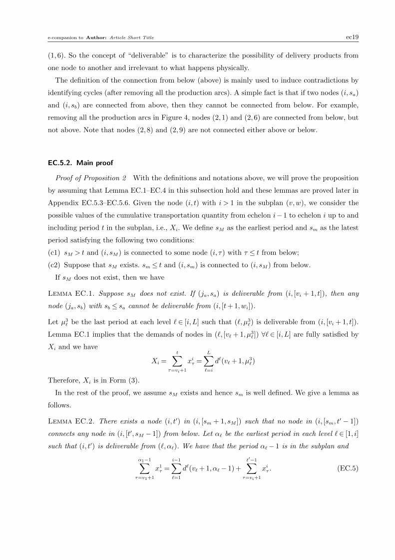
e-companion to Author: Article Short Title ec19

(1,6). So the concept of “deliverable” is to characterize the possibility of delivery products from

one node to another and irrelevant to what happens physically.

The definition of the connection from below (above) is mainly used to induce contradictions by

identifying cycles (after removing all the production arcs). A simple fact is that if two nodes (i, sa)

and (i, sb) are connected from above, then they cannot be connected from below. For example,

removing all the production arcs in Figure 4, nodes (2,1) and (2,6) are connected from below, but

not above. Note that nodes (2,8) and (2,9) are not connected either above or below.

EC.5.2. Main proof

Proof of Proposition 2 With the definitions and notations above, we will prove the proposition

by assuming that Lemma EC.1–EC.4 in this subsection hold and these lemmas are proved later in

Appendix EC.5.3–EC.5.6. Given the node (i, t) with i > 1 in the subplan (v,w), we consider the

possible values of the cumulative transportation quantity from echelon i−1 to echelon i up to and

including period t in the subplan, i.e., Xi. We define sM as the earliest period and sm as the latest

period satisfying the following two conditions:

(c1) sM > t and (i, sM) is connected to some node (i, τ) with τ ≤ t from below;

(c2) Suppose that sM exists. sm ≤ t and (i, sm) is connected to (i, sM) from below.

If sM does not exist, then we have

Lemma EC.1. Suppose sM does not exist. If (ja, sa) is deliverable from (i, [vi + 1, t]), then any

node (ja, sb) with sb ≤ sa cannot be deliverable from (i, [t+ 1,wi]).

Let µ3` be the last period at each level ` ∈ [i,L] such that (`,µ3

`) is deliverable from (i, [vi + 1, t]).

Lemma EC.1 implies that the demands of nodes in (`, [v` + 1, µ3` ]) ∀` ∈ [i,L] are fully satisfied by

Xi and we have

Xi =t∑

τ=vi+1

xiτ =L∑`=i

d`(v` + 1, µ3`)

Therefore, Xi is in Form (3).

In the rest of the proof, we assume sM exists and hence sm is well defined. We give a lemma as

follows.

Lemma EC.2. There exists a node (i, t′) in (i, [sm + 1, sM ]) such that no node in (i, [sm, t′ − 1])

connects any node in (i, [t′, sM − 1]) from below. Let α` be the earliest period in each level `∈ [1, i]

such that (i, t′) is deliverable from (`,α`). We have that the period α`− 1 is in the subplan and

α1−1∑τ=v1+1

x1τ =

i−1∑`=1

d`(v` + 1, α`− 1) +t′−1∑

τ=vi+1

xiτ . (EC.5)

ec20 e-companion to Author: Article Short Title

Based on Lemma EC.2, we consider two cases that t < t′ or t′ ≤ t. Case (i): Suppose t < t′. We

have

Lemma EC.3. If (ja, sa) is deliverable from (i, [t+ 1, t′− 1]), then

(a) any node (ja, sb) with sb ≤ sa is not deliverable from (i, [t′,wi]), and

(b) any node (ja, sb) with sb ≥ sa is not deliverable from (i, [vi + 1, t]).

Lemma EC.3 shows that if nodes (`, η1` ) and (`,µ1

`) are deliverable from (i, [t+ 1, t′− 1]) for some

`∈ [i,L] and η1` , µ

1` ∈ [v` + 1,w`], then the demands of nodes (`, η1

` ), . . . , (`,µ1`) are fully satisfied by∑t′−1

τ=t+1 xiτ . Apparently, if a node at level ` is deliverable from (i, [t+ 1, t′ − 1]), then there exist

nodes at level `−1 that are deliverable from (i, [t+1, t′−1]). Therefore, there exist j1 ∈ [i−1,L−1],

and η1` , µ

1` ∈ [v` + 1,w`] ∀`∈ [i, j1] such that

t′−1∑τ=t+1

xiτ =

j1∑`=i

d`(η1` , µ

1`). (EC.6)

Note that j1 <L. If not, then a node at the final level L is deliverable from a node, say (i, τ), in

(i, [t+ 1, t′ − 1]). Hence, the delivery path will intersect with the path that connects (i, sm) and

(i, sM) from below, which implies that (i, τ) and (i, sm) are connected from below. Since τ < t′ ≤ sMand satisfies condition (c1), it violates the choice of sM . Therefore, we have j1 < L. We allow

j1 = i−1 when∑t′−1

τ=t+1 xiτ = 0, in case t′ = t+1 and [t+1, t′−1] = ∅. Combining (EC.5) and (EC.6),

we have

α1−1∑τ=v1+1

x1τ =

i−1∑`=1

d`(v` + 1, α`− 1) +t′−1∑

τ=vi+1

xiτ

=i−1∑`=1

d`(v` + 1, α`− 1) +t∑

τ=vi+1

xiτ +t′−1∑τ=t+1

xiτ

=i−1∑`=1

d`(v` + 1, α`− 1) +t∑

τ=vi+1

xiτ +

j1∑`=i

d`(η1` , µ

1`),

which implies

Xi =t∑

τ=vi+1

xiτ =

α1−1∑τ=v1+1

x1τ −

i−1∑`=1

d`(v` + 1, α`− 1)−j1∑`=i

d`(η1` , µ

1`),

where∑α1−1

τ=v1+1 x1τ is the production quantity of a sequence of periods and we can relabel α`− 1 as

µ1` ∀`∈ [1, i− 1]. This is exactly Form (1).

Case (ii): Suppose t′ ≤ t. We have

Lemma EC.4. If (ja, sa) is deliverable from (i, [t′, t]), then

(c) any node (ja, sb) with sb ≤ sa is not deliverable from (i, [t+ 1,wi]), and

e-companion to Author: Article Short Title ec21

(d) any node (ja, sb) with sb ≥ sa is not deliverable from (i, [vi + 1, t′− 1]).

Note that Lemma EC.4 is similar to Lemma EC.3. Then there exist j2 ∈ [i− 1,L− 1], and η2` , µ

2` ∈

[v` + 1,w`] ∀`∈ [i, j2] such thatt∑

τ=t′

xiτ =

j2∑`=i

d`(η2` , µ

2`) (EC.7)

Note that j2 <L. If not, then a node at the final level L is deliverable from a node, say (i, τ), in

(i, [t′, t]). Hence, the delivery path will intersect with the path that connecting (i, sm) and (i, sM)

from below, which implies that (i, τ) and (i, sM) are connected from below. Since τ ≥ t′ > sm and

satisfies condition (c2), it violates the choice of sm. Therefore, we have j2 <L. Combining (EC.5)

and (EC.7), we have

α1−1∑τ=v1+1

x1τ =

i−1∑`=1

d`(v` + 1, α`− 1) +t′−1∑

τ=vi+1

xiτ

=i−1∑`=1

d`(v` + 1, α`− 1) +t∑

τ=vi+1

xiτ −t∑

τ=t′

xiτ

=i−1∑`=1

d`(v` + 1, α`− 1) +t∑

τ=vi+1

xiτ −j2∑`=i

d`(η2` , µ

2`),

which implies

Xi =t∑

τ=vi+1

xiτ =

α1−1∑τ=v1+1

x1τ −

i−1∑`=1

d`(v` + 1, α`− 1) +

j2∑`=i

d`(η2` , µ

2`)

where∑α1−1

τ=v1+1 x1τ is the production quantity of a sequence of periods and we can relabel α`− 1 as

µ2` ∀`∈ [1, i− 1]. This is exactly Form (2).

Next, we prove all the lemmas in the Proof of Proposition 2 in the following subsections.

EC.5.3. Proof of Lemma EC.1

We will prove the lemma by introducing contradictions. Let (ja, sa) be deliverable from (i, s1) with

s1 ∈ [vi + 1, t] and (ja, sb) be deliverable from (i, t1) with t1 > t as in Figure EC.11. The solid lines

indicate the deliverable property. Apparently, they must intersect as shown in Figure EC.11. Since

t1 satisfies condition (c1), it contradicts to the assumption that sM does not exist.

EC.5.4. Proof of Lemma EC.2

Proof of Lemma EC.2 First we will show that t′ can be found by an algorithm of repeating the

following two steps. We denote t0 = sM to simplify the notation. At each iteration k, starting from

k= 0, we

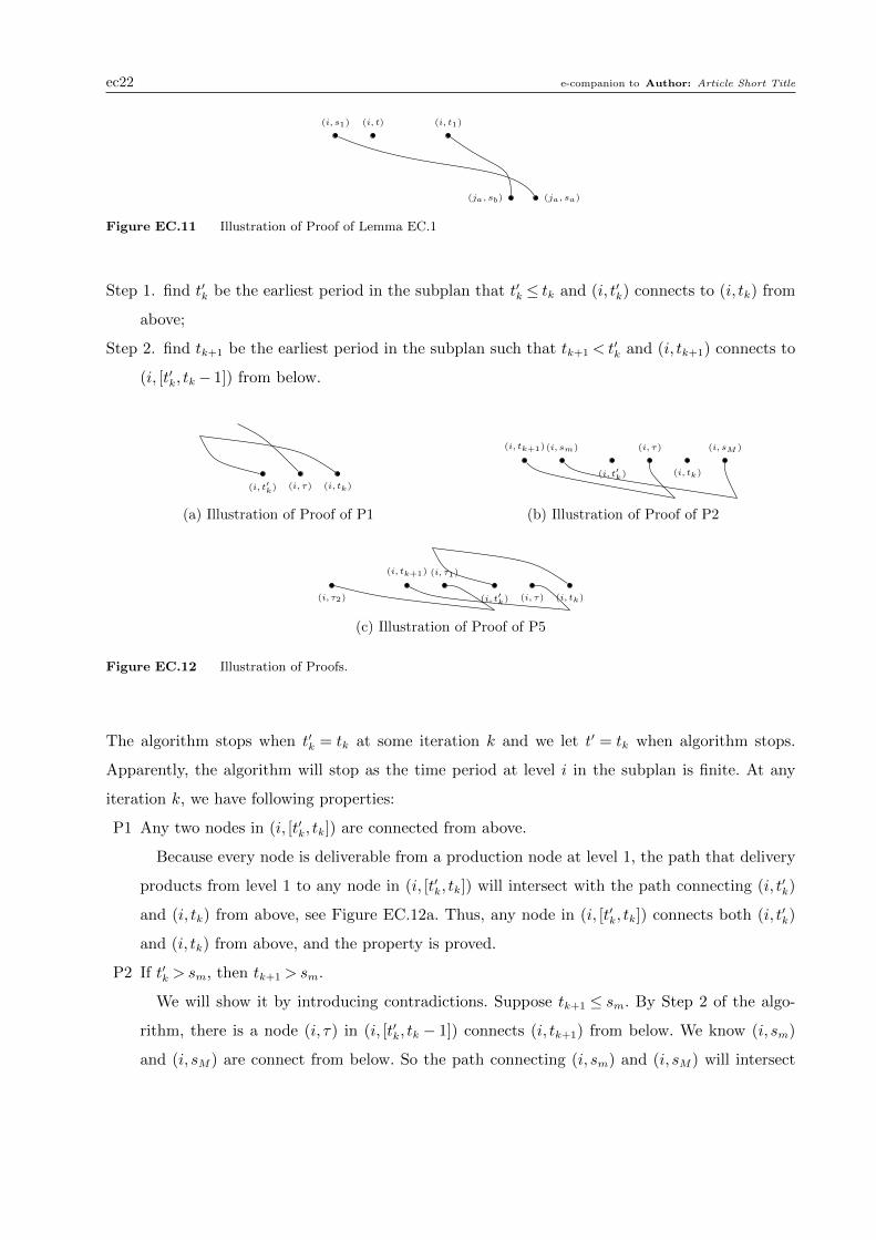
ec22 e-companion to Author: Article Short Title

(i, s1) (i, t1)(i, t)

(ja, sa)(ja, sb)

Figure EC.11 Illustration of Proof of Lemma EC.1

Step 1. find t′k be the earliest period in the subplan that t′k ≤ tk and (i, t′k) connects to (i, tk) from

above;

Step 2. find tk+1 be the earliest period in the subplan such that tk+1 < t′k and (i, tk+1) connects to

(i, [t′k, tk− 1]) from below.

(i, tk)(i, t′k) (i, τ)

(a) Illustration of Proof of P1

(i, tk)(i, t′k)

(i, τ)(i, tk+1)(i, sm) (i, sM )

(b) Illustration of Proof of P2

(i, tk)

(i, tk+1)

(i, t′k) (i, τ)(i, τ2)

(i, τ1)

(c) Illustration of Proof of P5

Figure EC.12 Illustration of Proofs.

The algorithm stops when t′k = tk at some iteration k and we let t′ = tk when algorithm stops.

Apparently, the algorithm will stop as the time period at level i in the subplan is finite. At any

iteration k, we have following properties:

P1 Any two nodes in (i, [t′k, tk]) are connected from above.

Because every node is deliverable from a production node at level 1, the path that delivery

products from level 1 to any node in (i, [t′k, tk]) will intersect with the path connecting (i, t′k)

and (i, tk) from above, see Figure EC.12a. Thus, any node in (i, [t′k, tk]) connects both (i, t′k)

and (i, tk) from above, and the property is proved.

P2 If t′k > sm, then tk+1 > sm.

We will show it by introducing contradictions. Suppose tk+1 ≤ sm. By Step 2 of the algo-

rithm, there is a node (i, τ) in (i, [t′k, tk − 1]) connects (i, tk+1) from below. We know (i, sm)

and (i, sM) are connect from below. So the path connecting (i, sm) and (i, sM) will intersect

e-companion to Author: Article Short Title ec23

with the path connecting (i, τ) and (i, tk+1), see Figure EC.12b. If t < τ , τ satisfies the condi-

tion (c1). Note that τ < tk ≤ sM . It contradicts with the choice of sM . If τ ≤ t, τ satisfies the

condition (c2) and τ ≥ t′k > sm, which contradicts with the choice of sm. So tk+1 > sm.

P3 Any node in (i, [t′k, tk]) is connected to a node in (i, [t′0, t0− 1]) if t′0 < t0(= sM).

This is true when k= 0 because of the property (P1). Suppose it is true for k− 1. Because

of the property (P1), any two nodes in (i, [t′k, tk]) are connected from above. Also, node (i, tk)

connects to (i, [t′k−1, tk−1− 1]) from below. So the property holds.

P4 If tk > sm, then t′k > sm.

If the algorithm stops at k = 0, then t′ = t′0 = t0 = sM . The property holds obviously. Now

we assume that the algorithm does not stop at k = 0. Thus, t′0 < t0. Suppose the property is

not true and t′k ≤ sm, i.e., node (i, sm) is in (i, [t′k, tk]). The Property (P3) shows that (i, sm)

connects to (i, [t′0, t0 − 1]). Together with (i, sM) connects to (i, [t′0, t0 − 1]) from above based

on Property (P1) and (i, sm) and (i, sM) are connected from below, we obtain a cycle in the

subplan which is a contradiction. So t′k > sm.

P5 No node in (i, [tk+1, tk− 1]) connects to nodes in (i, [sm, tk+1− 1]) from below.

Because t0 = sM > sm. From Property (P2) and (P4), we know the algorithm will stop at a

period later than sm. So the interval [sm, tk+1−1] in Property (P5) is valid. Since [tk+1, tk−1] =

[tk+1, t′k − 1]∪ [t′k, tk − 1], we consider two cases for the node set (i, [tk+1, tk − 1]) in Property

(P5). If any node in (i, [t′k, tk − 1]) connects to nodes in (i, [sm, tk+1− 1]) from below, then it

violates the choice of tk+1 in Step 2. If a node (i, τ1) in (i, [tk+1, t′k−1]) connects to a node (i, τ2)

in (i, [sm, tk+1−1]) from below, see Figure EC.12c, the connecting path will intersect with the

path that connecting (i, tk+1) to (i, τ) from below, where the node (i, τ) is in (i, [t′k, tk − 1]).

Now, (i, τ) can connects a node (i, τ2) in (i, [sm, tk+1−1]) from below. It violates the choice of

tk+1.

In the proof of Property (P5), we have already showed that the algorithm stops at t′ ∈ [sm+1, sM ].

Since t′ ≤ tk+1, Property (P5) implies that there is no node in (i, [tk+1, tk − 1]) connects to nodes

in (i, [sm, t′ − 1]) from below for any k. Note that

⋃k[tk+1, tk − 1] = [t′, sM − 1]. Thus, there is no

node in (i, [sm, t′− 1]) connects node in (i, [t′, sM − 1]) from below.

Now, with α` ∀`∈ [1, i] defined in the lemma, we will prove two claims,

1. αi = t′;

2. xiτ = 0 ∀τ ∈ [αi−1, αi− 1];

First, we show that αi = t′. Certainly, αi ≤ t′ by the definition of αi and deliverable property.

Suppose αi < t′. Because (i, t′) is deliverable from (i,αi), the delivery path is on level i connecting

(i,αi) to (i, t′). Thus (i,αi) and (i, t′) are connected from above and the Step 1 should not stop,

which is a contradiction. So, αi = t′.

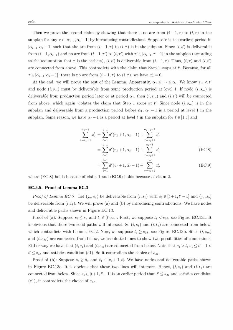
ec24 e-companion to Author: Article Short Title

Then we prove the second claim by showing that there is no arc from (i− 1, τ) to (i, τ) in the

subplan for any τ ∈ [αi−1, αi− 1] by introducing contradictions. Suppose τ is the earliest period in

[αi−1, αi− 1] such that the arc from (i− 1, τ) to (i, τ) is in the subplan. Since (i, t′) is deliverable

from (i−1, αi−1) and no arc from (i−1, τ ′) to (i, τ ′) with τ ′ ∈ [αi−1, τ−1] in the subplan (according

to the assumption that τ is the earliest), (i, t′) is deliverable from (i− 1, τ). Thus, (i, τ) and (i, t′)

are connected from above. This contradicts with the claim that Step 1 stops at t′. Because, for all

τ ∈ [αi−1, αi− 1], there is no arc from (i− 1, τ) to (i, τ), we have xiτ = 0.

At the end, we will prove the rest of the Lemma. Apparently, α1 ≤ · · · ≤ αi. We know sm < t′

and node (i, sm) must be deliverable from some production period at level 1. If node (i, sm) is

deliverable from production period later or at period α1, then (i, sm) and (i, t′) will be connected

from above, which again violates the claim that Step 1 stops at t′. Since node (i, sm) is in the

subplan and deliverable from a production period before α1, α1 − 1 is a period at level 1 in the

subplan. Same reason, we have α`− 1 is a period at level ` in the subplan for `∈ [1, i] and

α1−1∑τ=v1+1

x1τ =

i−1∑`=1

d`(v` + 1, α`− 1) +

αi−1−1∑τ=vi+1

xiτ

=i−1∑`=1

d`(v` + 1, α`− 1) +

αi−1∑τ=vi+1

xiτ (EC.8)

=i−1∑`=1

d`(v` + 1, α`− 1) +t′−1∑

τ=vi+1

xiτ (EC.9)

where (EC.8) holds because of claim 1 and (EC.9) holds because of claim 2.

EC.5.5. Proof of Lemma EC.3

Proof of Lemma EC.3 Let (ja, sa) be deliverable from (i, s1) with s1 ∈ [t+ 1, t′− 1] and (ja, sb)

be deliverable from (i, t1). We will prove (a) and (b) by introducing contradictions. We have nodes

and deliverable paths shown in Figure EC.13.

Proof of (a): Suppose sb ≤ sa and t1 ∈ [t′,wi]. First, we suppose t1 < sM , see Figure EC.13a. It

is obvious that those two solid paths will intersect. So (i, s1) and (i, t1) are connected from below,

which contradicts with Lemma EC.2. Now, we suppose t1 ≥ sM , see Figure EC.13b. Since (i, sm)

and (i, sM) are connected from below, we use dotted lines to show two possibilities of connections.

Either way we have that (i, s1) and (i, sm) are connected from below. Note that s1 > t, s1 ≤ t′−1<

t′ ≤ sM and satisfies condition (c1). So it contradicts the choice of sM .

Proof of (b): Suppose sb ≥ sa and t1 ∈ [vi + 1, t]. We have nodes and deliverable paths shown

in Figure EC.13c. It is obvious that those two lines will intersect. Hence, (i, s1) and (i, t1) are

connected from below. Since s1 ∈ [t+1, t′−1] is an earlier period than t′ ≤ sM and satisfies condition

(c1), it contradicts the choice of sM .

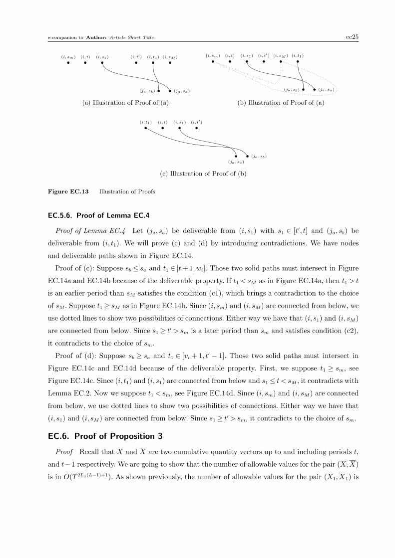
e-companion to Author: Article Short Title ec25

(i, s1) (i, t′) (i, sM )(i, t1)(i, t)(i, sm)

(ja, sa)(ja, sb)

(a) Illustration of Proof of (a)

(i, s1) (i, sM ) (i, t1)(i, t′)(i, sm) (i, t)

(ja, sa)(ja, sb)

(b) Illustration of Proof of (a)

(i, t′)(i, s1)(i, t)(i, t1)

(ja, sb)

(ja, sa)

(c) Illustration of Proof of (b)

Figure EC.13 Illustration of Proofs

EC.5.6. Proof of Lemma EC.4

Proof of Lemma EC.4 Let (ja, sa) be deliverable from (i, s1) with s1 ∈ [t′, t] and (ja, sb) be

deliverable from (i, t1). We will prove (c) and (d) by introducing contradictions. We have nodes

and deliverable paths shown in Figure EC.14.

Proof of (c): Suppose sb ≤ sa and t1 ∈ [t+ 1,wi]. Those two solid paths must intersect in Figure

EC.14a and EC.14b because of the deliverable property. If t1 < sM as in Figure EC.14a, then t1 > t

is an earlier period than sM satisfies the condition (c1), which brings a contradiction to the choice

of sM . Suppose t1 ≥ sM as in Figure EC.14b. Since (i, sm) and (i, sM) are connected from below, we

use dotted lines to show two possibilities of connections. Either way we have that (i, s1) and (i, sM)

are connected from below. Since s1 ≥ t′ > sm is a later period than sm and satisfies condition (c2),

it contradicts to the choice of sm.

Proof of (d): Suppose sb ≥ sa and t1 ∈ [vi + 1, t′ − 1]. Those two solid paths must intersect in

Figure EC.14c and EC.14d because of the deliverable property. First, we suppose t1 ≥ sm, see

Figure EC.14c. Since (i, t1) and (i, s1) are connected from below and s1 ≤ t < sM , it contradicts with

Lemma EC.2. Now we suppose t1 < sm, see Figure EC.14d. Since (i, sm) and (i, sM) are connected

from below, we use dotted lines to show two possibilities of connections. Either way we have that

(i, s1) and (i, sM) are connected from below. Since s1 ≥ t′ > sm, it contradicts to the choice of sm.

EC.6. Proof of Proposition 3

Proof Recall that X and X are two cumulative quantity vectors up to and including periods t,

and t−1 respectively. We are going to show that the number of allowable values for the pair (X,X)

is in O(T 2L1(L−1)+1). As shown previously, the number of allowable values for the pair (X1,X1) is

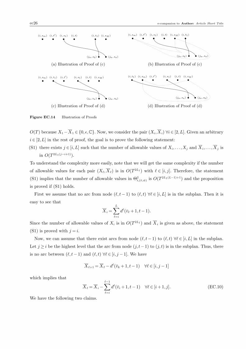
ec26 e-companion to Author: Article Short Title

(i, s1) (i, t1) (i, sM )(i, t)(i, sm) (i, t′)

(ja, sa)(ja, sb)

(a) Illustration of Proof of (c)

(i, s1) (i, sM ) (i, t1)(i, t)(i, sm) (i, t′)

(ja, sa)(ja, sb)

(b) Illustration of Proof of (c)

(i, t′) (i, t) (i, sM )(i, s1)(i, t1)(i, sm)

(ja, sb)(ja, sa)

(c) Illustration of Proof of (d)

(i, t′) (i, t) (i, sM )(i, s1)(i, t1) (i, sm)

(ja, sb)(ja, sa)

(d) Illustration of Proof of (d)

Figure EC.14 Illustration of Proofs

O(T ) because X1−X1 ∈ 0, ε,C. Now, we consider the pair (Xi,X i) ∀i∈ [2,L]. Given an arbitrary

i∈ [2,L] in the rest of proof, the goal is to prove the following statement:

(S1) there exists j ∈ [i,L] such that the number of allowable values of Xi, . . . ,Xj and X i, . . . ,Xj is

in O(T 2L1(j−i+1)).

To understand the complexity more easily, note that we will get the same complexity if the number

of allowable values for each pair (X`,X`) is in O(T 2L1) with ` ∈ [i, j]. Therefore, the statement

(S1) implies that the number of allowable values in Θ2t,(v,w) is O(T 2L1(L−1)+1) and the proposition

is proved if (S1) holds.

First we assume that no arc from node (`, t− 1) to (`, t) ∀` ∈ [i,L] is in the subplan. Then it is

easy to see that

X i =L∑`=i

d`(v` + 1, t− 1).

Since the number of allowable values of Xi is in O(T 2L1) and X i is given as above, the statement

(S1) is proved with j = i.

Now, we can assume that there exist arcs from node (`, t− 1) to (`, t) ∀`∈ [i,L] in the subplan.

Let j ≥ i be the highest level that the arc from node (j, t−1) to (j, t) is in the subplan. Thus, there

is no arc between (`, t− 1) and (`, t) ∀`∈ [i, j− 1]. We have

X`+1 =X`− d`(vk + 1, t− 1) ∀`∈ [i, j− 1]

which implies that

X` =X i−`−1∑`=i

d`(vi + 1, t− 1) ∀`∈ [i+ 1, j]. (EC.10)

We have the following two claims.

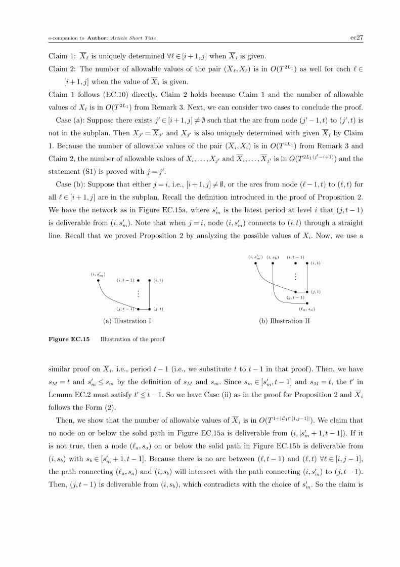
e-companion to Author: Article Short Title ec27

Claim 1: X` is uniquely determined ∀`∈ [i+ 1, j] when X i is given.

Claim 2: The number of allowable values of the pair (X`,X`) is in O(T 2L1) as well for each ` ∈

[i+ 1, j] when the value of X i is given.

Claim 1 follows (EC.10) directly. Claim 2 holds because Claim 1 and the number of allowable

values of X` is in O(T 2L1) from Remark 3. Next, we can consider two cases to conclude the proof.

Case (a): Suppose there exists j′ ∈ [i+ 1, j] 6= ∅ such that the arc from node (j′− 1, t) to (j′, t) is

not in the subplan. Then Xj′ =Xj′ and Xj′ is also uniquely determined with given X i by Claim

1. Because the number of allowable values of the pair (X i,Xi) is in O(T 4L1) from Remark 3 and

Claim 2, the number of allowable values of Xi, . . . ,Xj′ and X i, . . . ,Xj′ is in O(T 2L1(j′−i+1)) and the

statement (S1) is proved with j = j′.

Case (b): Suppose that either j = i, i.e., [i+ 1, j] 6= ∅, or the arcs from node (`− 1, t) to (`, t) for

all ` ∈ [i+ 1, j] are in the subplan. Recall the definition introduced in the proof of Proposition 2.

We have the network as in Figure EC.15a, where s′m is the latest period at level i that (j, t− 1)

is deliverable from (i, s′m). Note that when j = i, node (i, s′m) connects to (i, t) through a straight

line. Recall that we proved Proposition 2 by analyzing the possible values of Xi. Now, we use a

(i, s′m)

(i, t− 1) (i, t)

...

(j, t− 1) (j, t)

(a) Illustration I

(i, s′m) (i, t− 1)

(i, t)

...

(j, t− 1)

(j, t)

(`a, sa)

(i, sb)

(b) Illustration II

Figure EC.15 Illustration of the proof

similar proof on X i, i.e., period t− 1 (i.e., we substitute t to t− 1 in that proof). Then, we have

sM = t and s′m ≤ sm by the definition of sM and sm. Since sm ∈ [s′m, t− 1] and sM = t, the t′ in

Lemma EC.2 must satisfy t′ ≤ t− 1. So we have Case (ii) as in the proof for Proposition 2 and X i

follows the Form (2).

Then, we show that the number of allowable values of X i is in O(T 1+|L1∩[1,j−1]|). We claim that

no node on or below the solid path in Figure EC.15a is deliverable from (i, [s′m + 1, t− 1]). If it

is not true, then a node (`a, sa) on or below the solid path in Figure EC.15b is deliverable from

(i, sb) with sb ∈ [s′m + 1, t− 1]. Because there is no arc between (`, t− 1) and (`, t) ∀` ∈ [i, j − 1],

the path connecting (`a, sa) and (i, sb) will intersect with the path connecting (i, s′m) to (j, t− 1).

Then, (j, t− 1) is deliverable from (i, sb), which contradicts with the choice of s′m. So the claim is

ec28 e-companion to Author: Article Short Title

correct and no demand of node at or below level j is served from node (i, [s′m+1, t−1]). Therefore,∑t−1

τ=t′ xiτ in (EC.7) (we modify the index t in (EC.7) to t− 1 while replicating the same proof on

X i) do not include demands at level j or any level lower than level j, i.e., j2 < j. Hence, the number

of allowable values of X i is in O(T 1+|L1∩[1,j−1]|).

Suppose j > i. Note that the number of allowable values of Xj and Xi are in O(TL1+|L1∩[j,L−1]|)

and O(T 2L1) respectively from Remark 3. Xj is uniquely determined after X i because of Claim

1. The number of allowable values of Xi,Xj,X i,Xj is in O(T 4L1) since 1 + |L1 ∩ [1, j− 1]|+ |L1 ∩[j,L − 1]| ≤ L1. Based on Claim 2, the number of allowable values of the pairs (X`,X`) are in

O(T 2L1) ∀`∈ [i+ 1, j− 1] when the value of X i is given. Hence the statement (S1) is proved.

Now we consider j = i. Since the number of allowable values of Xi is in O(TL1+|L1∩[j,L−1]|) by

Remark 3, The number of allowable values of Xi,X i is in O(T 2L1) and the statement (S1) holds

with j = i.

EC.7. Proof of Theorem 7 and Corollary 1

Proof of Theorem 7 Given a relaxed subplan (v, w), slightly different from Section 2.3.3, we

define ψ(v,w)(t,X1,X2), with a time period t ∈ [v1, T ], as the the optimal cost where the demand

D1(0, v) is satisfied, plus the optimal cost of having X1 as the cumulative production quantity

up to and including period t in the subplan, and X2 as the cumulative transportation quantity

from echelon 1 to echelon 2 up to and including period t in the subplan. The goal is to determine

the value of ψ(T,T)(T,0,0). Because of ZIO property and the proof of Proposition EC.1, we have

X2 =D2(v, µ) for some µ∈Ω2,t(v, w) (see the definition in Section EC.2). Without loss of generality,

we can redefine the notation as ψ(v,w)(t,X1, µ). Following the dynamic programming recursions

(11), we have

ψ(v,w)(t,X1, µ) = minX1−X1∈0,ε,Cand η∈Ω2,t(v,µ)

ψ(v,w)(t− 1,X1, η) + p1t (X1−X1)

+h1t (X1−D2(v, µ)− d1(v1 + 1,min(t, w1))) +F2,t(η, µ) (EC.11)

where F2,t(η, µ) and Ω2,t(v, µ) are defined in Section EC.2. We have boundary conditions

φ(v,w)(t,0) = φ(u,v)(t,D1(u, v) ·1) ∀u≤ v and relaxed subplan (u, v), and φ(0,0)(0,0) = 0.

Note that F2,t(η, µ), for all t, η, µ, can be determined in O(LT 3L1+1) as shown in Section 2.2.1.

With given v, w, t,X1, µ, η and the value of F2,t(η, µ), the recursion can be evaluated in constant

time. The complexity is O(T 4L1+2 +LT 3L1+1). Therefore, Theorem 7 is proved.

Proof of Corollary 1 In the case of 2-CLS-F, v, w, µ, η are equivalent to scalars because only

their second components are not fixed to 0 and µ2 ≥ t. As shown by van Hoesel et al. (2005), we

must have X2 =X2 when µ2 > t because no speculative motives implies that we should transport

as late as possible. So η= µ when µ2 > t. This will reduce the complexity to O(T 5).

e-companion to Author: Article Short Title ec29

EC.8. Proof of Theorem 8

We will prove the theorem by induction. As we showed before, when 0 = k0 = k1 = · · · = kL−1 ≤

kL ≤ n. The theorem holds and the 1-echelon inequality is valid. Thus, we assume that (L− 1)-

echelon inequality is valid when 0 = k0 = k1 ≤ · · · ≤ kL ≤ n. We partition the proof into two parts

by considering whether the set t∈ S1 : x1t > 0 is empty.

First, we suppose t ∈ S1 : x1t > 0 = ∅. Note that, for 0 = k0 = k1 ≤ · · · ≤ kL ≤ n, we have

[ki−1 + 1, ki] ⊆ Ti ⊆ [1, ki] and Si ⊆ Ti ∀i ∈ [2,L]. The induction hypothesis gives us an (L − 1)-

echelon inequality

∑t∈[1,k2]\S2

x2t +

∑t∈S2

φ2ty

2t +

L∑i=3

∑t∈Ti\Si

xit +∑t∈Si

φityit

≥ L∑i=2

di(1, ki)

We have

∑t∈T1\S1

x1t +

∑t∈S1

φ1ty

1t +

L∑i=2

∑t∈Ti\Si

xit +∑t∈Si

φityit

− L∑i=1

di(1, ki)

≥∑

t∈[1,k1]

x1t +

L∑i=2

∑t∈Ti\Si

xit +∑t∈Si

φityit

− L∑i=1

di(1, ki) (EC.12)

≥∑

t∈[1,k1]

x2t + d1(1, k1) +

L∑i=2

∑t∈Ti\Si

xit +∑t∈Si

φityit

− L∑i=1

di(1, ki)

=∑

t∈[1,k1]

x2t +

∑t∈T2\S2

x2t +

∑t∈S2

φ2ty

2t +

L∑i=3

∑t∈Ti\Si

xit +∑t∈Si

φityit

− L∑i=2

di(1, ki)

≥∑

t∈[1,k2]\S2

x2t +

∑t∈S2

φ2ty

2t +

L∑i=3

∑t∈Ti\Si

xit +∑t∈Si

φityit

− L∑i=2

di(1, ki)≥ 0

where (EC.12) holds because t ∈ S1 : x1t > 0= ∅ and π0 ≥ 0. So the m-echelon inequality holds

when t∈ S1 : x1t > 0= ∅.

Now, we assume t∈ S1 : x1t > 0 6= ∅ and let s= mint∈ S1 : x1

t > 0. We define some parameters

as follows

• k2 = maxt≥ s− 1 : [s, t]⊆ T2, T 2 = [1, k2] and S2 = [s, k2]∩S2;

• ki = maxt≥ ki−1 : [ki−1 + 1, t]⊆ Ti, T i = Ti ∩ [1, ki] and Si = Si ∩ [1, ki] ∀i∈ [3,L].

Before showing the validity of the m-echelon inequality, we will introduce three Lemmas. The

first Lemma shows certain conditions hold among ki, T i and Si ∀i ∈ [2,L]. Then, the reduction

hypothesis can be applied to obtain a (L− 1)-echelon inequality based on those parameters.

Lemma EC.5. We have 0 = k0 = k1 ≤ · · · ≤ km ≤ n, [ki−1 + 1, ki] ⊆ T i ⊆ [1, ki] and Si ⊆ T i ∀i ∈

[2,L].

ec30 e-companion to Author: Article Short Title

Proof of Lemma EC.5 By the definition of ki ∀i∈ [2,L], it is clear that 0 = k0 = k1 ≤ · · · ≤ kL ≤n by introducing two dummy parameters k0 and k1. Also, following the definition, it is obvious that

[1, k2]⊆ T 2 ⊆ [1, k2] and Si ⊆ T i ∀i∈ [2,L]. Since [ki−1, ki]⊆ Ti, we have [ki−1 + 1, ki]⊆ Ti∩ [1, ki] =

T i ⊆ [1, ki] ∀i∈ [3,L].

Because of Lemma EC.5, we have a valid inequality

L∑i=2

∑t∈T i\Si

xit +∑t∈Si

φi

tyit

≥ L∑i=2

di(1, ki) (EC.13)

where φi

t =∑m

`=i d`(αi`t + 1, β

i

`t) such that αiit = t− 1, βi

it = maxτ ≥ t− 1 : [t, τ ]⊆ T i],

αi`t = maxτ ≥ αi`−1,t : [αi`−1,t + 1, τ ]⊆ T ` and βi

`t = maxτ ≥ βi`−1,t : [βi

`−1,t + 1, t]⊆ T `

In the next two Lemmas, we will build the connections between inequality (EC.13) and multiechelon

inequality.

Lemma EC.6. We have

1. T 2\S2 ⊆ [1, s− 1]∪ (T2\S2) and T i\Si ⊆ Ti\Si ∀i∈ [3,L],

2. φ1s = d1(s, k1) +

∑m

`=2 d`(k` + 1, k`)

Proof of Lemma EC.6 First, we will prove 1. Note that [s, k2]⊆ T2 and S2 = [s, k2]∩S2. Thus

T 2\S2 = [1, k2]\S2 = [1, s− 1]∪ ([s, k2]\S2)⊆ [1, s− 1]∪ (T2\S2).

and, for i∈ [3,L],

T i\Si = (Ti ∩ [1, ki])\(Si ∩ [1, ki])⊆ Ti\Si

Now we will prove 2. By the definition in Theorem 8, we have φ1s =

∑m

`=1 d`(α1

`s + 1, β1`s), where

αs and βs follow the iterative definition. Note that

α11s = s− 1 and α1

2s = maxτ ≥ s− 1 : [s, τ ]⊆ T2= k2.

Because α1`s and k` ∀`∈ [3,L] have the same iterative definition, we have α1

`s = k` ∀`∈ [2,L]. Since

T1 = [1, k1], we have β1`t = k` ∀t∈ T1, hence β1

`s = k`. Therefore, we have φ1s = d1(s, k1)+

∑L

`=2 d`(k`+

1, k`).

Lemma EC.7. φit = φi

t ∀i∈ [2,L], t∈ Si.

Proof of Lemma EC.7 First, we will show that αi`t = αi`t ∀` ∈ [i,L]. By the definition, αiit =

αiit = t− 1. Suppose αi`−1,t = αi`−1,t for some `∈ [i+ 1,L]. We have

αi`t = maxτ ≥ αi`−1,t : [αi`−1,t + 1, τ ]⊆ T `= maxτ ≥ αi`−1,t : [αi`−1,t + 1, τ ]⊆ T `

= maxτ ≥ αi`−1,t : [αi`−1,t + 1, τ ]⊆ T` ∩ [1, k`]

= maxτ ≥ αi`−1,t : [αi`−1,t + 1, τ ]⊆ T`= αi`t (EC.14)

e-companion to Author: Article Short Title ec31

Because αi`−1,t = αi`−1,t ≤ k`−1, we get αi`,t ≤ k` based on the definition that [k`−1 + 1, k`]⊆ T` and

k` + 1 /∈ T`. So (EC.14) holds. Thus, we have αi`t = αi`t ∀`∈ [i,L].

Then we will show that β22t = β

2

2t. We have

β2

2t = maxτ ≥ j− 1 : [j, τ ]⊆ T 2= maxτ ≥ j− 1 : [j, τ ]⊆ [1, k2]

= maxτ ≥ j− 1 : [j, τ ]⊆ [s, k2] (EC.15)

= maxτ ≥ j− 1 : [j, τ ]⊆ T2= β22t (EC.16)

(EC.15) holds because t∈ S2 ⊆ [s, k2]. (EC.16) holds because [s, k2]⊆ T2 and k2 + 1 /∈ T2.

At last, we will show that βi`t = βi

`t ∀i∈ [2,L], `∈ [i,m]. If βi`−1,t = βi

`−1,t and `≥ 3, then we have

βi

`t = maxτ ≥ βi`−1,t : [βi

`−1,t + 1, τ ]⊆ T `

= maxτ ≥ βi`−1,t : [βi`−1,t + 1, τ ]⊆ T `

= maxτ ≥ βi`−1,t : [βi`−1,t + 1, τ ]⊆ T` ∩ [1, k`]

= maxτ ≥ βi`−1,t : [βi`−1,t + 1, τ ]⊆ T`= βi`t (EC.17)

Because βi`−1,t = βi

`−1,t ≤ k`−1, we get βi`,t ≤ k` based on the definition that [k`−1 + 1, k`]⊆ T` and

k` + 1 /∈ T`. So (EC.17) holds.

Note that we already have β22j = β

2

2j. Thus, (EC.17) shows that β2`j = β

2

`j ∀`∈ [2,L]. If we denote

βii−1,j = βi

i−1,j = j− 1 for i≥ 3, then (EC.17) shows that βi`j = βi

`j ∀i∈ [3,L], `∈ [i,L]. In summary,

we have all αs and βs equal. Therefore, we have φij = φi

j ∀i∈ [2,L], j ∈ Si.

Now, we are ready to show that the inequality (13) is valid. We have

∑t∈T1\S1

x1t +

∑t∈S1

φ1ty

1t +

L∑i=2

∑t∈Ti\Si

xit +∑t∈Si

φityit

− L∑i=1

di(1, ki)

≥∑

j∈[1,s−1]

x1j +φ1

s +L∑i=2

∑j∈Ti\Si

xij +∑j∈Si

φijyij

− L∑i=1

di(1, ki)

≥∑

j∈[1,s−1]

x2j + d1(1, s− 1) +φ1

s +L∑i=2

∑j∈Ti\Si

xij +∑j∈Si

φijyij

− L∑i=1

di(1, ki)

≥ d1(1, s− 1) +φ1s +

L∑i=2

∑j∈T i\Si

xij +∑j∈Si

φijyij

− L∑i=1

di(1, ki) (EC.18)

≥ d1(1, s− 1) +φ1s +

L∑i=2

∑j∈T i\Si

xij +∑j∈Si

φi

jyij

− L∑i=1

di(1, ki) (EC.19)

≥ d1(1, s− 1) + d1(s, k1) +L∑`=2

d`(k` + 1, k`) +L∑i=2

di(1, ki)−L∑i=1

di(1, ki)≥ 0

ec32 e-companion to Author: Article Short Title

(EC.18) hold because of Lemma EC.6, (EC.19) hold because of Lemma EC.7, and the last inequality

holds because of induction hypothesis (EC.5). Therefore, the multiechelon inequality in Theorem

8 is valid.