MULTIDISCIPLINARY OPTIMIZATION OF A LIGHTWEIGHT TORPEDO STRUCTURE SUBJECTED TO

UNDERWATER EXPLOSION

A thesis submitted in partial fulfillment of the requirements for the degree of

Master of Science in Engineering

By

Rajesh Kalavalapally B.Tech., Jawaharlal Nehru Technology University, India 2002

2005 Wright State University

1

2

ABSTRACT

Kalavalapally, Rajesh, M. S. Engineering., Department of Mechanical and Materials Engineering, Wright State University, 2005. Multidisciplinary Optimization of a Lightweight Torpedo Structure Subjected to Underwater Explosion Undersea weapons, including torpedoes, need to be designed to survive extreme loading

conditions such as underwater explosions (UNDEX). The response of a lightweight

torpedo when subjected to an underwater explosion is an important criterion for

multidisciplinary design. This research obtains the UNDEX response of torpedo structure

using both metallic and composite material models. The pressure wave resulting from an

underwater explosion was modeled using similitude relations, and it was assumed to be a

spherical wave. A surface based interaction procedure was used to model the fluid-

structure interaction involved during the UNDEX event. The finite element package

ABAQUS was used to model the UNDEX and the fluid-structure interaction (FSI)

phenomena, which are critical for accurate evaluation of torpedo stress levels.

This research also investigates the effect of structural stiffeners on the

performance of a lightweight torpedo. A final configuration was obtained for the torpedo

that had minimum weight and was least sensitive to small manufacturing variations in the

dimensions of the stiffeners. For a stiffened metallic torpedo, an optimal configuration

with least possible weight for a given level of safety from an explosion at a critical

distance is obtained. The response of a composite lightweight torpedo model is also

obtained and structural optimization is performed to achieve the minimum weight subject

to the required safety levels. It is observed that a composite model was safer and lighter

than the stiffened metallic torpedo.

3

TABLE OF CONTENTS

1. Introduction ……………………………………………………………… 1

1.1 Background …………………………………………………………. 2

1.2 Scope of Work…………………………………………………......... 5

2. Modeling of the Torpedo and Surrounding Fluid……………………….. 7

2.1 Metallic Lightweight Torpedo Modeling……………………………. 7

2.2 Composite Torpedo Modeling………………………………………. 8

2.3 Boundary Conditions………………………………………………….11

2.4 Fluid Modeling……………………………………………………….. 13

3. Underwater Explosion & Pressure Wave Distribution…………………….15

3.1 UNDEX Phenomenon…………………………………………………15

3.2 Similitude Relations (Pressure vs. Time)…………………………….. 16

3.3 Pressure Wave Distribution on the Structure………………………… 18

4. Modeling Fluid-Structure Interaction Phenomenon……………………….20

5. Surface-based Interaction Procedure…………………………………….. 22

6. Composite Failure Measures………………………………………………25

7. Optimization Problem Formulation……………………………………….29

7.1 Composite Lightweight Torpedo…………………………………….. 29

7.2 Metallic Lightweight Torpedo……………………………………….. 29

7.3 Method of Feasible Directions……………………………………….. 30

8. Results and Discussion……………………………………………………31

8.1 Metallic Flat Plate……………………………………………………..32

8.2 Metallic Lightweight Torpedo……………………………………….. 34

4

8.3 Stiffened Lightweight Torpedo………………………………………. 38

8.4 Composite Flat Plate Response……………………………………. 46

8.5 Composite Lightweight Torpedo Response………………………… 49

9. Optimization Results…………………………………………………….. 51

9.1 Composite Lightweight Torpedo……………………………………. 51

9.2 Metallic Lightweight Torpedo………………………………………. 52

10. Conclusions and Future work ……………………………………………. 55

10.1 Conclusions ……………………………………………………… 55

10.2 Future work………………………………………………………. 56

Appendix A …………………………………………………………….…58

Appendix B …………………………………………………………….…60

Appendix C …………………………………………………………….…63

Appendix D …………………………………………………………….…74

References …………………………………………………………….... 76

5

LIST OF FIGURES

Figure 2.1 Dimensions of lightweight torpedo model with stiffeners 8

Figure 2.2 Finite element model of a lightweight torpedo 9

Figure 2.3 Cross-section of a composite shell 10

Figure 2.4 Boundary conditions on the torpedo model to constrain

in axial direction 12

Figure 2.5 Boundary conditions on torpedo model to constrain from

rotating about its axis 13

Figure 2.6 Torpedo model surrounded by the fluid mesh 14

Figure 3.1 UNDEX phenomenon 15

Figure 3.2 Pressure vs. time history for 70.0 kg of HBX-1 charge,

standoff distance of 35.0 m 18

Figure 5.1 Fluid as “master” and structural surface as “slave” 23

Figure 8.1 Number of nodal points where pressure is applied 33

Figure 8.2 VonMises stress contour of a simply supported

flat plate subjected to UNDEX 34

Figure 8.3 Maximum von Mises stress for HBX-1 charge w.r.t.

standoff distance and explosive weight 37

Figure 8.4 Various stiffener positions explored 40

Figure 8.5 Maximum von Mises stress for 70 kg HBX-1 charge at

35.0 m w.r.t. longitudinal and ring stiffeners for case 1 41

Figure 8.6 Three different standoff positions considered 42

Figure 8.7 Stiffener combination vs maximum von Mises stress

6

for a 3 % change in the dimensions of the stiffeners 44

Figure 8.8 Mass of the lightweight torpedo model for different

longitudinal and ring stiffener combinations 45

Figure 8.9 Contour distribution of the tsai-hill failure criterion on

0 degree layer 47

Figure 8.10 Contour distribution of the tsai-hill failure criterion on

+45 degree layer 48

Figure 8.11 Contour distribution of the tsai-hill failure criterion on

-45 degree layer 48

Figure 8.12 Contour distribution of the tsai-hill failure criterion on

90 degree layer 48

Figure 8.13 Maximum stress failure index w.r.t standoff distance

and explosive weight 50

Figure 9.1 Optimum weight value with respect to ring and

longitudinal stiffener combination 54

7

LIST OF TABLES

Table 2.1 Material properties of carbon/epoxy 11

Table 3.1 Material constants for similitude relations 17

Table 8.1 Maximum von Mises stress at different standoff

distances for 70 kg of charge 36

Table 9.1 Optimized results for the composite lightweight

torpedo at 20 m standoff distance 52

Table 9.2 Optimized results for the composite lightweight

torpedo at 35 m standoff distance 52

Table 9.3 Optimized results for the metallic lightweight

torpedo at 35 m standoff distance for 3 different

stiffener combinations 53

Table A.1 Boundary condition parameters for radiation

boundary condition 59

8

ACKNOWLEDGEMENT

I would like to thank Dr. Ramana V. Grandhi, thesis advisor, for his constant

guidance and support throughout my graduate studies. I would also like to express my

gratitude to Dr. Ravi Penmetsa for his constant suggestions through out the course of the

study. I am grateful to both Dr. Grandhi and Dr. Ravi for their time and effort they

provided to me over the course of the research. The suggestions and guidance of Dr.

Vipperla Venkayya were of immense help and are highly appreciated. I would like to

express my gratitude to Dr. Ron Taylor for being part of my thesis committee. I

gratefully thank the editorial assistance of Brandy Foster and Chris Massey which were

of immense help in refining the document.

I would like to thank all my friends at CDOC and my roommates for providing

me the strength and support during my stay in the US.

This research work has been sponsored by the Office of Naval Research under the

contract N00014-03-1-0057. Dr. Kam Ng is the Program manager. Any opinions,

findings, conclusions, or recommendations expressed in this publication are those of the

author and do not necessarily reflect the views of the sponsors.

Finally, I would like to dedicate this work to my loving parents and my dearest

sister. Their love, support, and encouragement made it easier for me to reach my

academic goal.

9

1. Introduction

Torpedoes are self-propelled guided projectiles that operate underwater and are

designed to detonate on contact or in proximity to a target. They may be launched from

submarines, surface ships, helicopters, and fixed-wing aircrafts. They are also used as

parts of other weapons. The modern torpedoes enable submarines to defeat surface and

undersea threats, and they provide the surface ships the means to reach beneath the

surface and attack submarines. With these extensive abilities, the current generation

torpedoes are one of the fundamental drivers of 20th century naval warfare. While on their

mission, these undersea weapons are subjected to various external and internal loadings.

Hence during the design of these torpedo models, all the inter-conflicting disciplines need

to be considered. Also, the safety of these underwater weapons to different kinds of

external loadings is an important design criterion to consider. One of such importance is

the UNDerwater EXplosion (UNDEX) loading. The designed torpedoes need to be safe

from the near-miss of underwater explosions to successfully accomplish their mission.

Also, in many naval applications, reducing the weight of a structure without

compromising its strength and stiffness is considered one of the most important design

criteria. By virtue of their nature, composite materials provide exactly the above-

mentioned design criteria. In military applications, the use of composites allows for

enhancement in the stealth and survivability characteristics. Fiber-reinforced composite

materials are considered to have great potential in marine applications. The properties

10

that make them more advantageous over conventional materials such as steel, aluminum,

etc., for underwater applications are the high-strength and stiffness combined with their

light-weight, high-corrosion resistance, stealth, low observability to radiation, and less

transmission of mechanical noise from the structure to surrounding water. Hence a

successful design is the one that, while withstanding the loads produced due to UNDEX,

is of the least weight possible. Therefore, the current research focuses on designing a

least weight torpedo model by exploring the different materials used that can withstand

the UNDEX loading.

1.1 Background

Over the years the UNDEX response of underwater structures was obtained by

doing physical testing. Physical testing of a torpedo to determine its response to an

underwater explosion is an expensive process that can cause damage to the surrounding

environment. Therefore, the literature [1-3] shows the data collected from expensive

experimental tests on simple cylindrical shells and plate structures. The cost involved and

the environmental effects require exploration of numerical solution techniques that can

analyze the response of a torpedo subject to various explosions. Computational modeling

and response, if perfected, can effectively and accurately replace the experimental

procedures used to obtain the UNDEX response. Over the years, numerical simulations

have been developed to accurately capture the fluid structure interaction phenomenon

involved during an UNDEX event between the structure and the surrounding fluid

medium [4, 5].

11

An UNDEX simulation consists of obtaining the response of a finite-sized

structure (torpedo) subjected to a blast load when immersed in an infinite fluid medium

(sea or ocean). Due to the fact that UNDEX simulations use an infinite fluid medium,

researchers [6-9] have developed techniques that combine the benefits of both boundary

element and finite element methods. In this method, the structure was discritized into

finite elements, and the surrounding fluid medium was divided into boundary elements.

An approximate boundary integral technique, “Doubly Asymptotic Approximation”

(DAA), was used in this kind of incident wave problems and the boundary integral

program was developed.

Kwon and Cunningham [6] coupled an explicit finite element analysis code,

DYNA3D, and a boundary element code based on DAA, Underwater Shock Analysis

(USA), to obtain the dynamic responses of stiffened cylinder and beam elements. Also,

during the early 90s Kwon and Fox [7] studied the nonlinear dynamic response of a

cylinder subjected to side-on underwater explosion using both the experimental and

numerical techniques. Sun and McCoy [8] combined the finite element package

ABAQUS and a fluid-structure interaction code based on the DAA to solve an UNDEX

analysis of a composite cylinder. Similarly, there have been other researchers [9, 10] that

coupled a finite element code with a boundary element code such as DAA to capture the

fluid-structure interaction effect. Moreover, Cichocki, Adamczyk, and Ruchwa [11, 12]

have performed extensive research to obtain an UNDEX response of simple structures

and have implemented entire fluid-structure interaction phenomenon, pressure wave

distribution, and the radiation boundary conditions into the commercial finite element

package ABAQUS. In this research, the UNDEX response of a lightweight torpedo

12

subject to a side-on underwater explosion is analyzed using ABAQUS. The literature

review for the UNDEX response of the composite materials is detailed below.

Considering the background of composites, achievements in integrating the

laminated composite plates into the construction of naval ships and submarines are

outlined in the review paper by Mouritz et al. [13]. Seemingly, there has been extensive

research work done on laminated composite plate and cylindrical structures subject to the

most important and damaging loading underwater, UNDEX [14-18]. Mouritz [14]

observed the changes in the fatigue behavior of glass-reinforced polymer (GRP)

laminates when subjected to UNDEX loading. The shock response used in Ref [14] was

obtained experimentally using an UNDEX testing facility. Turkmen et al. [15] compared

the experimental results with the finite element results for a stiffened laminated

composite plate under blast loading in air. The effects of stiffener and loading conditions

on the dynamic response were observed in this paper. Similarly, Aslan et al. [16]

obtained the response of the fiber-reinforced laminated composite plates under low-

velocity impact through an experimental impact test and a dynamic finite element

analysis code. The results from the above papers suggest that when blast load is applied

in the transverse direction, the composite structures produce internal delamination. Dyka

and Badaliance [17] observed the damage in marine composites caused due to both the

air impact loading and UNDEX loading. The fluid structure interaction (FSI) effect,

which is critical while obtaining the UNDEX response, was considered in this paper.

Lam et al. [18] obtained the UNDEX response for a simply supported

laminated pipeline on the seabed. A fluid-structure interaction model was considered and

13

the response in the radial direction was found to be weaker. Also, parametric studies were

performed, including the standoff distance, charge weight, and length of the pipe.

1.2 Scope of Work

Current research focuses on analyzing an un-stiffened and a stiffened metallic

torpedo and composite model of the torpedo to determine their safe operating distances

given an explosion of a certain-sized charge. After verifying the hypothesis that the

stiffened torpedo would perform better, an optimal configuration of the torpedo was

determined. This configuration resulted in the minimum weight for a torpedo while

satisfying the constraints on safe operating distance. This design would also be relatively

insensitive to small variations in the stiffener dimensions of the torpedo. Robustness was

an important criterion for the torpedo design because, as mentioned by Penmetsa, et al.

[19], the variations in dimensions can reduce the reliability of the torpedo.

A parametric study was performed to obtain the stress response of the torpedo

model at different standoff distances in order to determine a safe distance for operation.

The safe distance calculations can be used to program the optimal path for interception.

For all of these standoff distances, the explosion was assumed to occur near the mid

section on the starboard side of the torpedo. This study was also extended to a stiffened

torpedo in order to compare its performance characteristics to that of an un-stiffened

torpedo. Since the stress distribution was dependent on the location of the explosion, the

position of the explosion was moved to the aft and forward sections of the torpedo. Once

all of these configurations were explored, an optimal configuration that minimized the

weight of the torpedo and maximized its survivability for all these cases was selected. All

14

the configurations were verified for a maximum von Mises stress constraint of 413 MPa,

which is the yield strength of aluminum. For all of the combinations that satisfy the stress

constraint, a 3% variation was assigned to the dimensions (width & breadth) of the

stiffeners to model manufacturing tolerances. This ensured that the sensitivity of the

stiffener dimensions to the stress was accounted for and that the final combination of ring

and longitudinal stiffeners was robust.

In all the above-cited references the UNDEX response was studied for

different kinds of structures, either composite or metallic. This research also aims at

applying the phenomenon of UNDEX analysis to obtain the safe distance for the torpedo

models to survive an explosion that was modeled using similitude relations. The other

aim of this research is to perform the structural optimization of the torpedo model for

reducing the overall weight of the structure. The configuration design, as described above,

for a torpedo subject to UNDEX was obtained prior to performing the structural

optimization. This part of the research compares the optimum metallic torpedo

characteristics with that of a composite laminated torpedo subjected to UNDEX loading.

A multidisciplinary optimization was performed by constraining the fundamental natural

frequency of the structure and the safety of the torpedo subject to UNDEX loading. In

this research work, before the response of the lightweight torpedo was obtained, the

UNDEX response of a simple structure, such as a laminated flat plate, was determined.

This has enabled the validation of the pressure distribution due to the explosion, and the

layer-by-layer response of the composite structure was also available.

15

2. Modeling of the Torpedo and the Surrounding Fluid

2.1 Metallic lightweight torpedo modeling

A lightweight torpedo similar to a MK-44 configuration was used to analyze and perform

a parametric study to obtain the safe operating distance. Also the optimized torpedo has

to fit in the existing torpedo tubes. The total mass of the torpedo model was considered to

be 243 kg, with a length of 2.42 m and a diameter of 0.32 m. The material chosen for the

torpedo structure was aluminum-2024. The torpedo was modeled using the shell elements,

and stiffeners, modeled using beam elements, were added in the longitudinal and the

radial directions to provide structural integrity. The shell thickness of the torpedo was

0.00635 m. The width and breadth of longitudinal and ring stiffeners were taken to be

0.015 m and 0.01 m, respectively. In order to model the mass of the components stored

within the compartments of the torpedo, concentrated masses were added to the torpedo

model. The structural mass of the torpedo model was about 43 kg, whereas the total mass

of an actual lightweight torpedo is around 243 kg. Therefore, the difference of 200 kg

was modeled as the mass of the internal components in each section and was distributed

equally along the length of the torpedo. The dimensions of the lightweight torpedo model

and the ring and longitudinal stiffeners can be seen in Figure 2.1.

16

Ring stiffeners Longitudinal stiffeners

Figure 2.1: Dimensions of lightweight torpedo model with stiffeners

The above-mentioned configuration was used to construct a finite element model

to perform the underwater explosion analysis. By performing the transient analysis, the

maximum von Mises stress for all of the time steps was obtained, which determined the

safe distance for the lightweight torpedo from the explosion.

2.2 Composite Torpedo Modeling

The dimensions of the composite model of the torpedo are similar to those of the

metallic one described above. A finite element model of a torpedo along with its

dimensions can be seen in Figure 2.2. The structure was modeled using the 1176 4-node

shell elements and 48 3-node shell elements. Composite material properties were given to

the outer shell elements. To represent the total mass of the various subsystems in a

lightweight torpedo, concentrated mass elements were placed at the nodes on the torpedo

shell. The overall reduction in weight of the torpedo was obtained due to the lighter

weight of the composite materials, without reducing the strength and stiffness.

0.32 m

2.42 m

17

2.42 m

0.32 m

Figure 2.2: Finite element model of a lightweight torpedo

A conceptual design was modeled by Adduri et al.[24] with a sandwich

honeycomb panel. This model consisted of a honeycomb core surrounded by fiber-

reinforced laminates that form the top and bottom shells. The cross-section of the shell

can be seen in Figure 2.3. The honeycomb increases the strength and rigidity of the

structure without a considerable increase in weight. Also, the direction of the fibers can

be changed to achieve higher strength in a particular direction. A reliability-based

optimization was presented to obtain the optimum stacking sequence and thickness of

each layer in the symmetric composite model. The optimum stacking sequence presented

in Ref[24] was [0/ 45/90]± s laminates with the honeycomb core in the middle. This same

configuration was used for this research. Each layer is defined by its thickness,

orientation angle, and the material properties. The honeycomb core is defined by its

thickness; the orientation angle was given zero degrees. An AS/3501 carbon/epoxy

unidirectional composite was chosen to model the laminates and a commercial grade

aluminum honeycomb was used to model the honeycomb. The material properties of

carbon/epoxy are given in Table 2.1. Since honeycomb only handles transverse shear,

only transverse shear moduli and the transverse shear strength are defined for material

properties of honeycomb, which are given below.

18

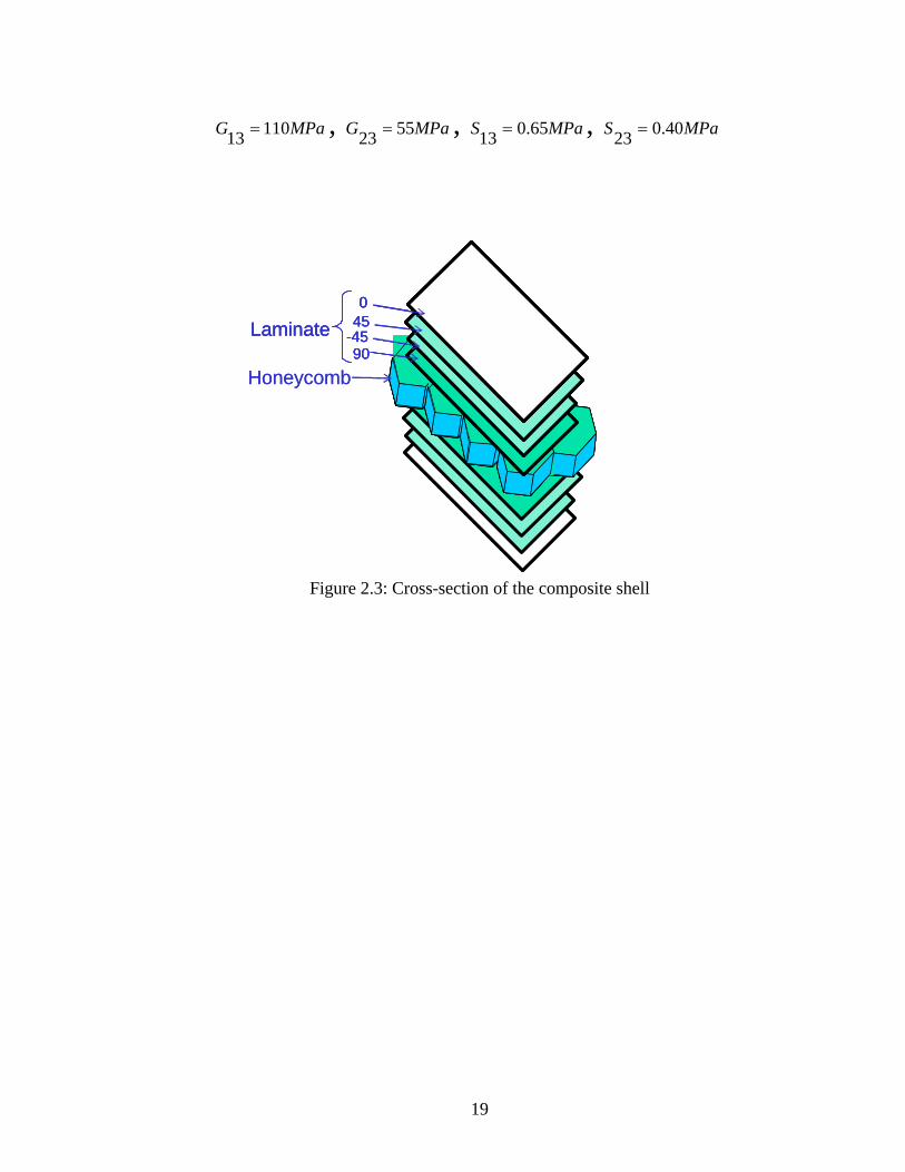
MPaG 11013 = , MPaG 5523 = , MPaS 65.013 = , MPaS 40.023 =

Honeycomb90

-4545Laminate0

Honeycomb9090

-45-454545Laminate0

Laminate00

Figure 2.3: Cross-section of the composite shell

19

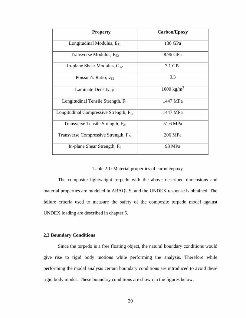
Property Carbon/Epoxy

Longitudinal Modulus, E11 138 GPa

Transverse Modulus, E22 8.96 GPa

In-plane Shear Modulus, G12 7.1 GPa

Poisson’s Ratio, ν12 0.3

Laminate Density, ρ 1600 kg/m3

Longitudinal Tensile Strength, F1t 1447 MPa

Longitudinal Compressive Strength, F1c 1447 MPa

Transverse Tensile Strength, F2t 51.6 MPa

Transverse Compressive Strength, F2c 206 MPa

In-plane Shear Strength, F6 93 MPa

Table 2.1: Material properties of carbon/epoxy

The composite lightweight torpedo with the above described dimensions and

material properties are modeled in ABAQUS, and the UNDEX response is obtained. The

failure criteria used to measure the safety of the composite torpedo model against

UNDEX loading are described in chapter 6.

2.3 Boundary Conditions

Since the torpedo is a free floating object, the natural boundary conditions would

give rise to rigid body motions while performing the analysis. Therefore while

performing the modal analysis certain boundary conditions are introduced to avoid these

rigid body modes. These boundary conditions are shown in the figures below.

20

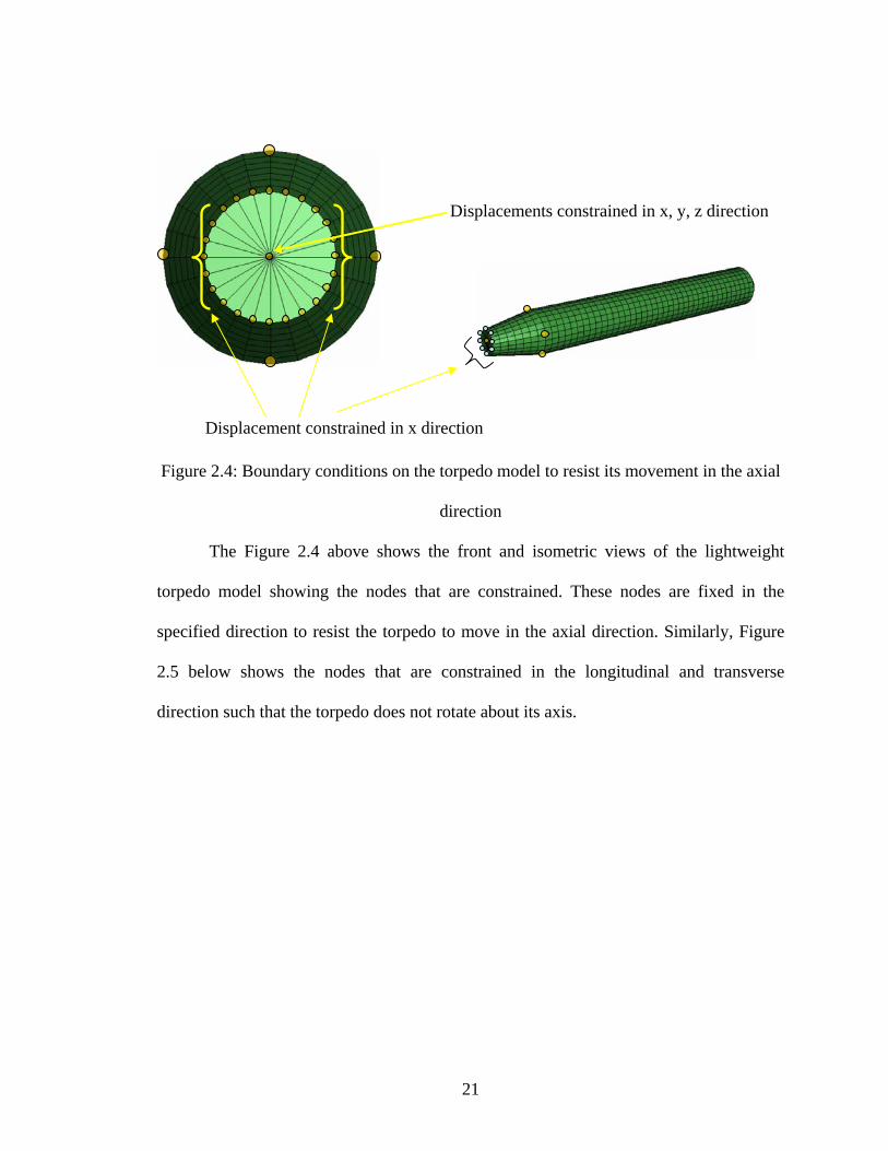
Displacement constrained in x direction

Displacements constrained in x, y, z direction

Figure 2.4: Boundary conditions on the torpedo model to resist its movement in the axial

direction

The Figure 2.4 above shows the front and isometric views of the lightweight

torpedo model showing the nodes that are constrained. These nodes are fixed in the

specified direction to resist the torpedo to move in the axial direction. Similarly, Figure

2.5 below shows the nodes that are constrained in the longitudinal and transverse

direction such that the torpedo does not rotate about its axis.

21

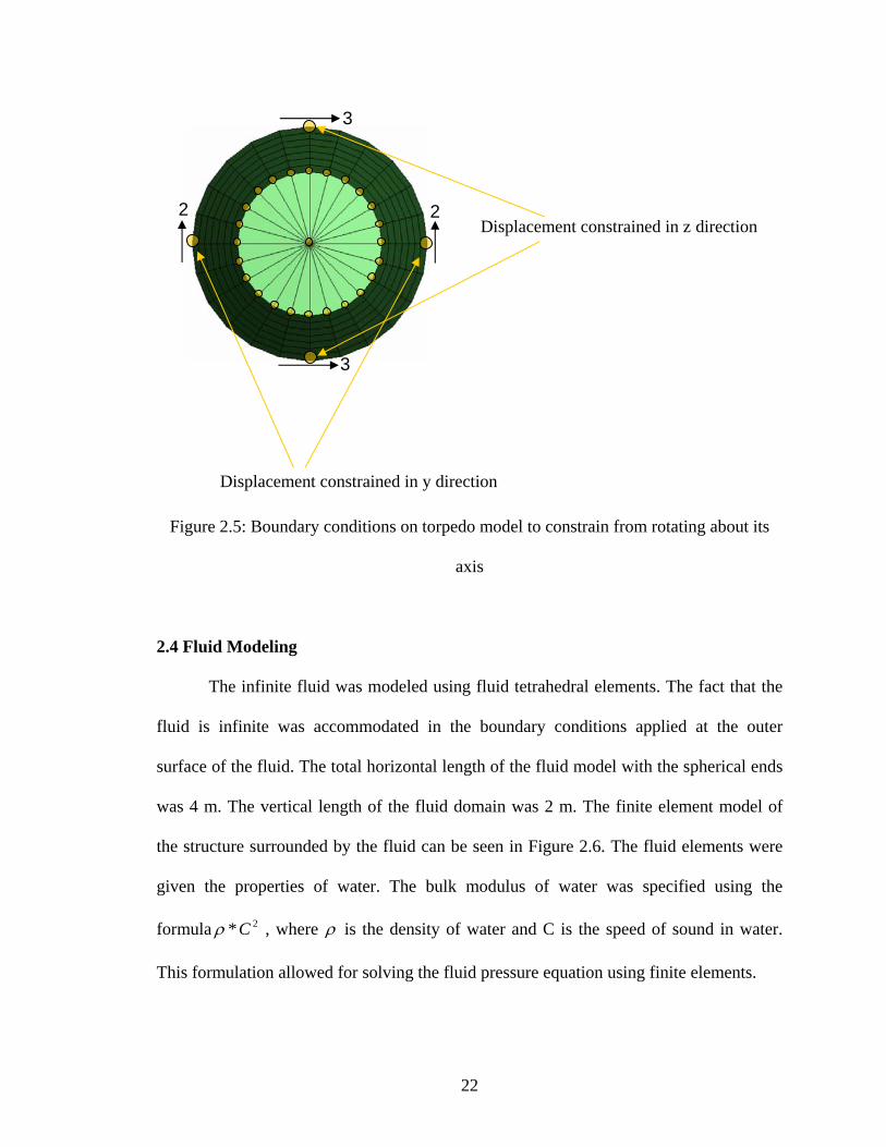
Displacement constrained in z direction

Displacement constrained in y direction

3

3

22

Figure 2.5: Boundary conditions on torpedo model to constrain from rotating about its

axis

2.4 Fluid Modeling

The infinite fluid was modeled using fluid tetrahedral elements. The fact that the

fluid is infinite was accommodated in the boundary conditions applied at the outer

surface of the fluid. The total horizontal length of the fluid model with the spherical ends

was 4 m. The vertical length of the fluid domain was 2 m. The finite element model of

the structure surrounded by the fluid can be seen in Figure 2.6. The fluid elements were

given the properties of water. The bulk modulus of water was specified using the

formula , where 2*Cρ ρ is the density of water and C is the speed of sound in water.

This formulation allowed for solving the fluid pressure equation using finite elements.

22

Figure 2.6: Torpedo model surrounded by the fluid mesh

The fluid-structure interaction phenomenon, discussed in detail in the coming

chapters, was applied at the common surface of the structural and the fluid finite element

mesh. An impedance-type radiation boundary condition was applied at the outer surface

of the fluid mesh to model the motion of fluid waves outside of the mesh. The size of the

fluid mesh depended on these conditions. The radiation boundary condition converges to

the exact condition in the limit as they become infinitely distant from the structure.

Therefore, these boundary conditions theoretically provided accurate results if the

distance between the structure and the radiating surface was one half of the longest

characteristic wave length. Based on the minimum distance requirements published in ref

[20] the existing model was adequate to obtain accurate results for the applied boundary

conditions. A brief explanation of the radiating boundary conditions is given in the

Appendix A.

23

3. Underwater Explosion & Pressure Wave Distribution

3.1 UNDEX phenomenon

An underwater explosion produces a great amount of gas and energy, resulting in

a shock wave [22]. This compression shock wave produced by the sudden increase of

pressure in the surrounding water travels radially away from the explosion with a velocity

approximately equal to the velocity of sound in water. The gases from the explosive form

a bubble that expands, reducing the gas pressure almost to zero. Due to the hydrostatic

pressure around the fully expanded bubble, it begins to collapse. Once the bubble is

compressed to a minimum radius, the high pressure causes the gases to detonate once

again, emitting a second shock wave. This second shock wave is called a “bubble pulse.”

Figure 3.1: UNDEX phenomenon

24

Figure 3.1 shows the different events occurring during the UNDEX event in a

pressure vs. time history plot. The under-pressure condition, as seen in the figure, is

caused by the back flow of the water toward the explosive due to contraction of the

bubble. Reflection of the shock wave off the bottom of the ocean is a compression wave

that adds additional load to the structure, and the reflection of the shock wave from the

free ocean surface causes a reduction in the pressure produced by the shock wave. In this

research, both the bubble pulse phenomenon and the reflection of the shock wave from

the bottom or the surface were not considered because they are less severe compared to

the initial shock wave. The initial shock wave was modeled as a spherical wave front,

which decays exponentially with time. The distribution of this shock wave onto the

torpedo was obtained using the incident pressure wave equations [20]. A detailed

explanation of the pressure wave distribution equations is given in the section below.

3.2 Similitude Relations (Pressure vs. Time):

To determine the safe distance for a torpedo beyond which it does not fail, the

pressure vs. time history of an explosive was required for different standoff distances

(distance between the structure and the explosive). The pressure vs. time history at a

particular standoff distance from the structure was obtained using the similitude relations

[21, 22].

The “similitude relations” accurately represent the far-field pressure profiles of an

explosive:

)(**),(1

τfRa

PtRPA

cc

+

⎥⎦⎤

⎢⎣⎡= (3.1)

25

c

cB

c

atv

Ra *

*⎥⎦⎤

⎢⎣⎡=τ (3.2)

,1,)( ≤= − ττ τef (3.3)

7,1749.08251.0)( 1805.0338.1 ≤+= −− ττ ττ eef (3.4)

In the above equations, is the pressure vs. time history, R is the distance from

the center of the explosive, is the radius of the spherical charge,

),( tRP

ca )(τf is an

exponential decay term, and , , A, and B are the constants that are associated with

the material of the charge. Some recommended values obtained from Ref [21] for these

constants are shown in Table 3.1.

cP cv

cν

0.23 0.14 1220 1.65 Pentolite (1.71 g/cc)

0.247 0.144 1170 1.58 HBX-1 (1.72 g/cc)

0.29 0.15 1470 1.71

0.185 0.18 1010 1.67 TNT (1.60 g/cc)

0.23 0.13 1240 1.45 TNT (1.60 g/cc)

0.18 0.13 992 1.42 TNT (1.52 g/cc)

B A , m/s Pc, GPa

HBX-1 (1.72 g/cc)

Charge

Table 3.1: Material constants for similitude equations

Once the far-field pressure data was obtained from the above relations for a

particular charge, it was applied as a transient load on the torpedo model. Figure 3.2

26

shows the pressure vs. time history that was applied on the torpedo model for a side-on

explosion in this research.

Figure 3.2: Pressure vs. time history for 70.0kg of HBX-1 charge,

standoff distance of 35.0 m

3.3 Pressure Wave Distribution on the Structure

The pressure load acting on the torpedo due to an underwater explosion changes

with respect to both time and space. The pressure vs. time history of an explosive is the

relation between pressure acting on the torpedo, as a spherical or plane wave, at the

standoff point (the point where the wave hits the structure first), and time. If the UNDEX

wave is considered as a spherical wave, the spatial distribution of a pressure wave on the

structure can be considered as a spherical distribution. This spherical distribution is

obtained using the “incident pressure wave equations” Ref [20]. The incident pressure

equation can be written as a separable solution to the scalar wave equation of the form

27

)()(),( jxtjI xptptxp ≡ (3.5)

where is specified through the pressure vs. time history at the standoff point x)(tpt o, and

is the spatial variation at a point and is given as )( jx xp jx

js

osjx xx

xxxp

−

−=)( (for spherical waves) (3.6)

= 1 (for plane waves) (3.7)

where is the specified source point (point of explosion). sx

By considering the time delay required for the wave to travel from the standoff point to

the point , it is found that jx

)()(),( jxo

ojtjI xp

cRR

tptxp−

−= (3.8)

)()( jxjt xpp τ≡ (3.9)

jsj

oso

xxR

xxR

−≡

−≡ (for spherical waves) (3.10)

( )( )os

sosjj xx

xxxxR

−

−−≡

. (for plane waves) (3.11)

In Equation 3.8, is the wave speed in the fluid, and 0c jτ is known as the “retarded time”

because it includes a shift corresponding to the time required for the wave to move from

the standoff point to . jx

28

4. Modeling Fluid-Structure Interaction Phenomenon

Obtaining the response of a torpedo to an underwater explosion involves

integration of the structural behavior and its effects on the surrounding fluid and vice-

versa. When the torpedo is exposed to a shock wave produced by an explosion, the

structure deforms and displaces fluid around it. The pressure distribution surrounding the

torpedo structure is also affected by the motion of the torpedo due to the shock wave.

This interaction between the fluid and the structure that exists until the vibration of the

system has decayed has to be modeled using coupled fluid-structure equations. A surface-

based procedure was used to enforce a coupling between the structural surface nodes and

the fluid surface nodes. The interaction was defined between the fluid and the torpedo

surface meshes. A detailed explanation of the surface-based interaction procedure is

given in the next chapter.

The reflections of the pressure wave after striking the structure are called

scattered waves, which needed to be taken into account while solving the finite element

equations. Therefore, the applied load used for solving the finite element equations

consisted of the sum of known incident and unknown scattered pressure wave

components. The incident wave field was the pressure vs. time history obtained, from the

similitude relations and the incident pressure wave equations, for the explosive.

The equations of motion used in this analysis are of the form:

pSuKuCuM Tfssss ][−=++ &&& (4.1)

29

TSpKpCpM fsfff ][=++ &&& (4.2)

SI ppp += (4.3)

where is the structural mass, is the structural damping matrix, is the

structural stiffness matrix, is the incident shock pressure wave, and is the

scattered pressure wave. In the above equations, u is the structural displacements, is

the mass of fluid, is the fluid damping matrix, is the fluid stiffness matrix, and the

transformation matrix integrates the fluid and structural degrees of freedoms and was

defined on all of the interacting fluid and structural surfaces. The fluid traction T in

Equation (4.2) is the quantity that describes the mechanism by which the fluid drives the

solid. By substituting equation (4.3) in (4.1) and (4.2), we obtain the fluid equation in

terms of the unknown scattered pressure term. The resulting equation was solved together

with Equation (4.1) to obtain the response of the torpedo structure.

sM sC sK

Ip Sp

fM

fC fK

fsS

30

5. Surface-based Interaction Procedure

The fluid-structure interaction capabilities of ABAQUS [20], such as solving for

the scattered term obtained due to reflection of the pressure wave and inclusion of the

coupling term in the structural and fluid equations, are used in this research work. In this

kind of coupled fluid-solid analysis, the fluid fields are strongly dependent on conditions

at the boundary of the fluid medium. The fluid medium consists of different sub-regions

where different conditions are specified, such as the radiation boundary condition to

model infinite fluid medium and fluid-structure interaction conditions.

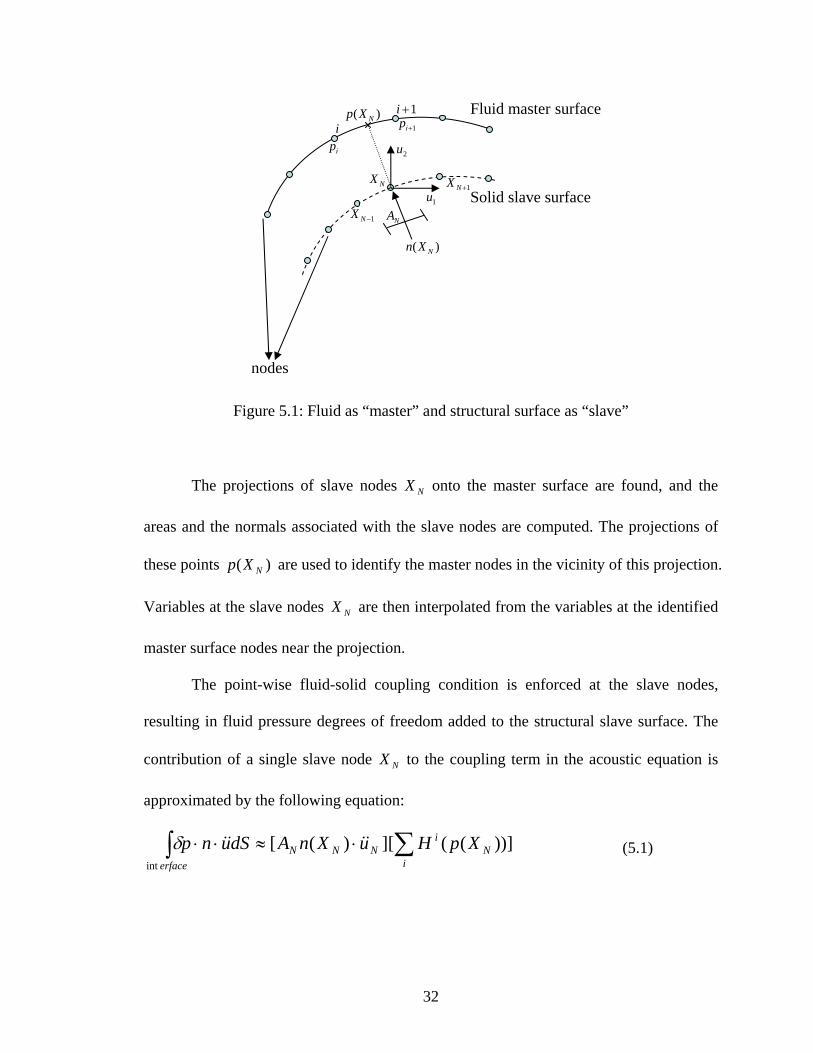
The fluid-structure interface is the region where the fluid medium is directly

coupled to the motion of the solid. The procedure uses a surface-based fluid-structure

medium interaction procedure, which is discussed below. The coupling is obtained by

designating the fluid and the structural surface nodes at the interface as the master and the

slave nodes, respectively. The slave side receives point tractions based on interpolation

with the shape functions from the master side. If the solid medium is designated as slave,

the values on this surface are constrained to equal values interpolated from the master

surface. Figure 5.1 illustrates the above theory.

31

Solid slave surface

Fluid master surface

nodes

1u

)( NXp

1−NX

1+NXNX

ip1+ip

2u

)( NXn

NA

i1+i

Figure 5.1: Fluid as “master” and structural surface as “slave”

The projections of slave nodes onto the master surface are found, and the

areas and the normals associated with the slave nodes are computed. The projections of

these points are used to identify the master nodes in the vicinity of this projection.

Variables at the slave nodes are then interpolated from the variables at the identified

master surface nodes near the projection.

NX

)( NXp

NX

The point-wise fluid-solid coupling condition is enforced at the slave nodes,

resulting in fluid pressure degrees of freedom added to the structural slave surface. The

contribution of a single slave node to the coupling term in the acoustic equation is

approximated by the following equation:

NX

))]((][)([int

Ni

iNN

erfaceN XpHuXnAdSunp ∑∫ ⋅≈⋅⋅ &&&&δ (5.1)

32

where is structural acceleration at the slave node, and are areas and

normals associated with the slave nodes, and are the interpolants on the

fluid master surface evaluated at projections . The summation is for all master

nodes “ ”, in the vicinity of the slave node projection. The entire coupling matrix is

computed by repeating this step for all the slave nodes.

Nu&& NA )( NXn

))(( Ni XpH

)( NXp

i

The contribution to the coupling term in the structural equation is approximated by

,))(( iNi

iN pXpHApdSnu ∑∫ ≈⋅⋅δ (5.2)

where is the pressure at master node “ i ” and the summation is for all the master nodes

in the vicinity of the slave node projection. By including the above terms into the fluid

and structural equations (4.1) & (4.2), the interaction between the fluid and structure is

modeled and these equations are solved together to obtain the response.

ip

33

6. Composite Failure Measures

To obtain the distance at which a laminated composite torpedo is safe for a

particular amount of charge, a failure criterion for the composite structure needs to be

known. This failure criterion has to take into account all types of deformations occurring

inside the composite. From the literature, one of the important types of failure occurring

when the composite structure is subjected to transverse dynamic loading is delamination,

which decreases the buckling and compressive strength of the composite structure.

Delmaination can be caused by the UNDEX loading normal to the direction of the fibers.

Failure of a composite is characterized by, the first ply failure criterion and the

progressive failure of composites [23]. In a laminate, stresses in the layers with different

orientations or different material properties are generally different because the stiffness

and strength of the lamina are different, depending on the direction in which the fibers are

oriented. Hence, some layers are likely to fail prior to the rest of the layers. This is known

as the first-ply failure criteria. But in some cases, the initiation of damage in one layer

does not mean the failure of the entire structure; the structure might still be able to

withstand additional load even after the occurrence of the initial damage. In such cases,

the effect the initial damage on the other layers in the laminates needs to be considered.

The number of failures keeps increasing progressively until the failure of an additional

laminate causes the failure of all the layers. This is known as progressive failure.

34

In most of the cases, it is not desirable to have local damage, since a small form of

damage, such as a transverse matrix crack, changes the elastic properties. Therefore, it is

assumed that the failure of the first ply is the failure of the composite. Estimating the

failure of the composite by the first ply criterion is conservative, but serves the purpose

because the initial matrix crack does not lead to the failure of the entire composite

structure.

Also, the failure of composite materials cannot be studied by simply considering

the principal stresses exceeding the yield stresses, as in the case of the isotropic materials.

Therefore, different failure theories that are based not just on principal normal stresses

and maximum shear stresses, but on the stresses in the material axes are considered. In

the case of unidirectional lamina, there are two material axes: direction one, which is

parallel to; the fibers and direction two, which is perpendicular to the fibers. The strength

parameters used in the failure theories, TX and , are the ultimate tensile and

compressive strengths along the longitudinal (Direction 1),

CX

TY and are the ultimate

tensile and compressive strengths along the transverse (Direction 2) direction of the fiber,

and is the ultimate in-plane shear strength. The different failure theories that define the

failure of a composite layer are as follows.

CY

S

Maximum Stress and Maximum Strain Criteria: These criteria verify if the maximum

stress or strain exceeds the allowable values of the stresses or strains in a particular

direction. These criteria are similar to the failure criteria for isotropic materials. These

failure criteria do not consider the interaction between the three different strength

parameters.

35

Tsai-Hill Criterion: This theory is based on the distortion energy failure theory of von

Mises yield criterion to anisotropic materials with equal strengths in tension and

compression. The failure index is calculated using Eq. (6.1) and the failure occurs when

the inequality is violated.

0.12

212

2

22

221

2

21 <++−=

STYTXTXFI

τσσσσ (6.1)

where 1σ and 2σ are the stresses along the longitudinal and transverse directions of the

fiber, 12τ is the shear stresses developed. The Tsai-Hill failure theory does not

distinguish between the compressive and tensile strength. Therefore, it is modified to

include the corresponding strengths, tensile or compressive, in the failure theory as

follows:

0.12

212

2

22

221

2

21 <++−=

SYXXFI

τσσσσ (6.2),

where TXX => ,01σ else CXX = and TYY => ,02σ else CYY =

Tsai-Wu Criterion: This is the most generalized criterion for orthotropic materials since it

distinguishes between the compressive and tensile strength of a lamina and the failure

index is calculated based on Eq. (6.3):

211222

212

22

21)11(2)11(1 σσ

τσσσσ F

SCYTYCXTXCYTYCXTXFI ++++−+−= (6.3)

where is the coefficient that reflects the interaction of the two normal stresses on the

failure. This is often determined experimentally.

12F

36

Hoffman Criterion: The interaction parameter was obtained empirically by Hoffman.

As per the Hoffman criterion,

12F

CXTXF

*21

12 = . By Substituting this value in Eq. (3),

the failure index is calculated based on Eq. (6.4):

0.1212

212

22

21)11(2)11(1 <−+++−+−=

CXTXSCYTYCXTXCYTYCXTXFI

σστσσσσ (6.4)

In the current research work, the stand-off distance at which the maximum failure

criteria defined by the modified Tsai-Hill criterion is just below 0.9 is considered as the

safe distance, and the distance at which it is just above is known as the critical distance.

37

7. Optimization Problem Formulation:

7.1 Composite lightweight torpedo model

An optimization problem is formulated to minimize weight of the structure

subject to various constraints. The constraints are to match the fundamental natural

frequency and also to ensure the safety of the torpedo model under UNDEX loading. The

UNDEX loading applied is at the critical distance where the structure fails. And, the

thicknesses of each layer are considered to be the design variables. The constraints for the

optimization are given in the equation below.

zH2.221 ≥ω , 9.0≤FI (7.1)

where 1ω is the fundamental natural frequency, and FI are the failure indices of each

layer in the element due to the UNDEX loading. The constant parameters are the standoff

distance, the source point, the orientation angle, and the ply sequence.

7.2 Metallic lightweight torpedo model

Similarly, an optimization problem was formulated to obtain an optimum

stiffened metallic torpedo model. As mentioned above, a configuration design was

performed for a stiffened torpedo model by performing different load case studies when

subjected to an underwater explosion. Hence, the optimization is performed only using

the safe combinations of stiffeners obtained by performing the case studies. The main

38

objective here is to minimize the weight of the structure. The constraints for the

optimization are given in the equation below.

zH2.221 ≥ω ,

Maximum vonMises stress Mpa413≤ (7.2)

where 1ω is the fundamental natural frequency, and the maximum vonMises stress is the

stress produced due to the explosion. The constant parameters are the standoff distance,

the source point, and the orientation of the stiffeners.

7.3 Method of Feasible Directions:

The above formulated optimization problems are solved using an optimization

tool called DOT (Design Optimization Tool). The method used in DOT is the Feasible

directions method. It is one of the types of direct search numerical method in which we

select a design to initiate the iterative process which is continued until no further moves

are possible and the optimality conditions are satisfied. The basic idea of the method is

from a feasible design )(kX , an improving feasible direction d(k) is determined such that

for a small step size α >0, the following two properties are satisfied: 1) the new design,

is feasible and 2) the new cost function is smaller than

the old one . Once d

)()()1( . kkk dXX α+=+ )( )1( +kXf

)( )(kXf (k) is determined, a line search is performed to determine

how far to proceed along the direction d(k) which leads to a new feasible design )1( +kX ,

and the process is repeated until the optimum is reached.

The above described optimization method is used in DOT to come up with

optimum value.

39

8. Results and Discussion

Obtaining the UNDEX response of the lightweight torpedo model was a complex

analysis, as it required integrating all of the above-described theories. By using the

commercial finite element package ABAQUS, which enables a seamless integration of

the above-discussed theories, the stress distribution on the torpedo was estimated. Before

obtaining the stress response of the torpedo, a simple structure, such as a flat plate, was

analyzed to verify the pressure distribution formulae applied in ABAQUS. After this

verification process, a torpedo model without stiffeners was analyzed for its stress

response when it was subjected to an underwater explosion. This analysis was performed

for different standoff distances and explosive weights in order to determine a safe

operating distance for each of the explosive configurations.

This initial weight vs. distance data was used to select a particular weight of depth

charge, 70 kg of HBX-1, and to extend the study to variation in the location of the

explosion. Once the torpedo was designed to survive a 70 kg HBX-1 from a particular

operating distance, a heavier charge could be used and the safe operating distance would

be moved back farther based on the distance vs. weight study performed earlier. Using

this information about the safe distance, the effect of adding stiffeners to the torpedo was

investigated. The configuration of stiffeners to be added to the torpedo to improve its

performance was obtained by considering its weight, robustness, and safety features. The

40

following section provides a detailed explanation of the results of different cases

explained above.

8.1 Metallic Flat Plate

UNDEX response of a simple structure, such as flat plate, was investigated in order to

verify the validity of the pressure distribution equations used [20]. A flat plate was

chosen to clearly visualize the propagation of the pressure wave with respect to time on

the nodal points of the plate, as given in the pressure distribution equations shown in

Chapter 3. The length of the plate was the same as the length of the torpedo with the

same thickness as the torpedo shell. The propagation of the pressure on the nodes can be

clearly depicted from the time vs number of nodes (experiencing pressure) plot in Figure

8.1. The tip of the shock wave hitting the structure at the centre first with maximum

amplitude and then advancing on to the other points on the structure with a decreased

magnitude of pressure comprised the sequence of events following the explosion wave

hitting the structure side-on.

41

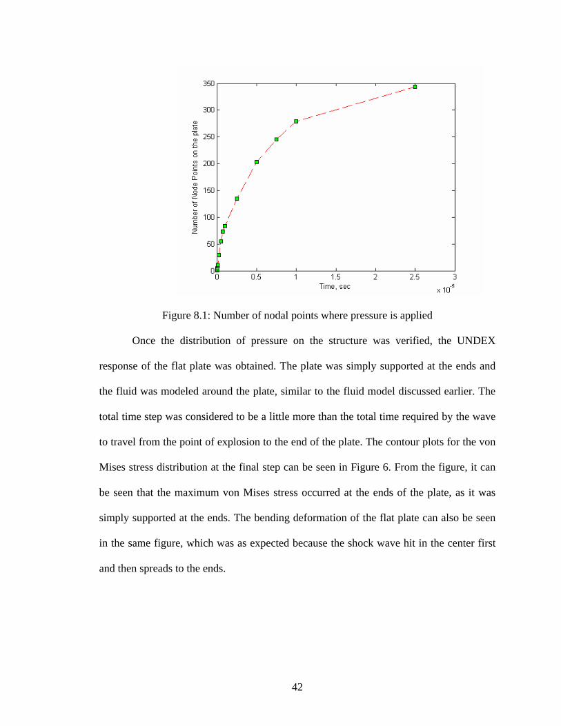
Figure 8.1: Number of nodal points where pressure is applied

Once the distribution of pressure on the structure was verified, the UNDEX

response of the flat plate was obtained. The plate was simply supported at the ends and

the fluid was modeled around the plate, similar to the fluid model discussed earlier. The

total time step was considered to be a little more than the total time required by the wave

to travel from the point of explosion to the end of the plate. The contour plots for the von

Mises stress distribution at the final step can be seen in Figure 6. From the figure, it can

be seen that the maximum von Mises stress occurred at the ends of the plate, as it was

simply supported at the ends. The bending deformation of the flat plate can also be seen

in the same figure, which was as expected because the shock wave hit in the center first

and then spreads to the ends.

42

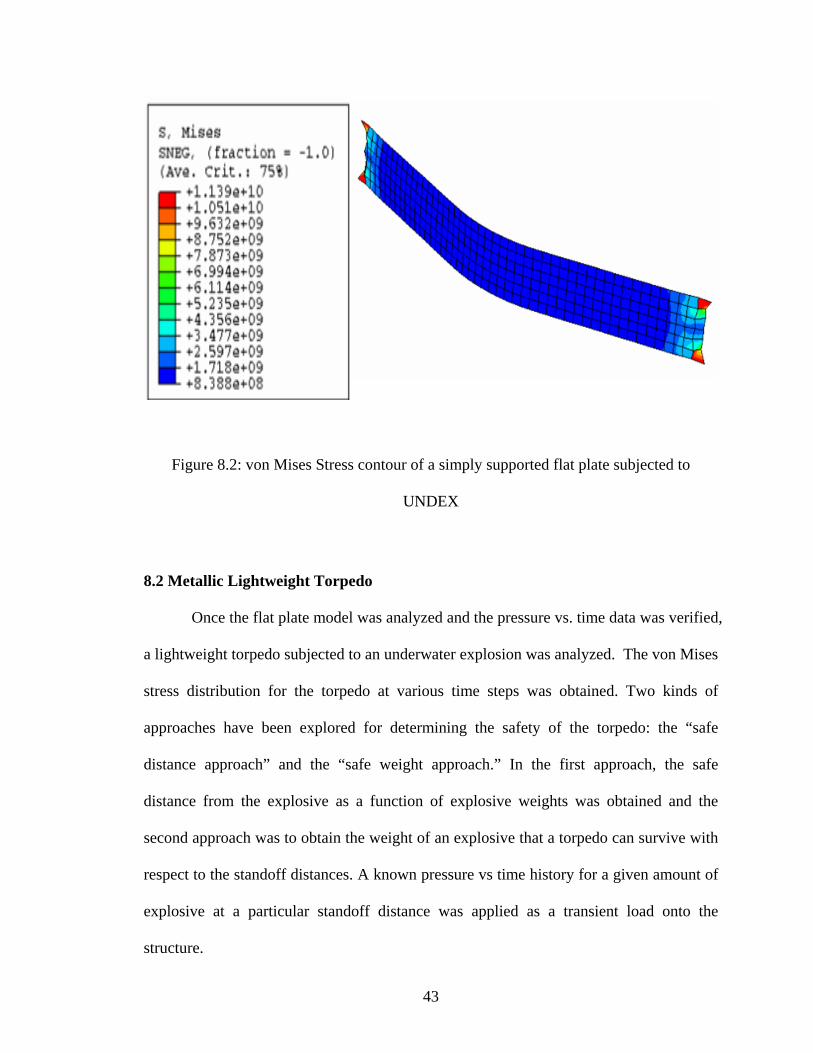
Figure 8.2: von Mises Stress contour of a simply supported flat plate subjected to

UNDEX

8.2 Metallic Lightweight Torpedo

Once the flat plate model was analyzed and the pressure vs. time data was verified,

a lightweight torpedo subjected to an underwater explosion was analyzed. The von Mises

stress distribution for the torpedo at various time steps was obtained. Two kinds of

approaches have been explored for determining the safety of the torpedo: the “safe

distance approach” and the “safe weight approach.” In the first approach, the safe

distance from the explosive as a function of explosive weights was obtained and the

second approach was to obtain the weight of an explosive that a torpedo can survive with

respect to the standoff distances. A known pressure vs time history for a given amount of

explosive at a particular standoff distance was applied as a transient load onto the

structure.

43

Similitude relations provided the pressure vs. time history data given the

explosive constants. In this paper, three kinds of explosives, HBX-1, Pentolite, and TNT,

were considered to obtain the maximum von Mises stress produced by the explosion.

When the maximum von Mises stress exceeded the yield strength of aluminum, the

structure was considered to fail. The standoff distance, just below the safe distance, at

which the structure fails was called the critical distance of the torpedo for that particular

charge. Table 8.1 shows the maximum von Mises stress at different standoff distances for

70 kg of HBX-1, Pentolite, and TNT charges. From the table, it can be seen that at a

distance of 35 m, HBX-1 had a maximum von Mises stress value of 440 Mpa, which is

more than the yield strength of aluminum. For TNT and Pentolite, failure occured at a 30

m standoff distance. The safe distance as estimated by this method was 40 m for HBX-1,

and 35 m for TNT and Pentolite. The critical distance for a torpedo without any stiffeners

was around 35.0 m. That is, the torpedo failed if it was closer than 35.0 m from the

explosive. This critical distance was for 70 kg of charge, and it was sensitive to the

amount of charge used for the explosion.

44

Table 8.1: Maximum von Mises stress at different standoff distances for

70 kg of charge

T es with

respect to the standoff distance and t X-1 charge. Any point on the above

plot giv

190.8 208.226.070.0

205.2 224.243.565.0

222.3 242.263.760.0

242.4 263.287.355.0

266.4 288.7315.550.0

295.7 318.348.645.0

332.7 357.390.040.0

379.1 405.439.535.0

443.9 471.504.330.0

532.3 563.596.425.0

662.0 693.732.520.0

862.4 904.4937.015.0

1316.2 1366.81401.810.0

2705.8 2755.55.0

TNT, MPa

Pentolite, MPa

HBX-1, MPa

Standoff Distance, m

8

0

3

0

5

5

3

4

6

4

2751.7

he plot in Figure 8.3 below shows the variation of the maximum von Mis

he amount of HB

es the maximum von Mises stress produced due to a certain amount of explosive

at a specific distance. It is possible to obtain the safe distance for the torpedo for a given

explosive charge using the above plot. As expected, the maximum stress occured at the

minimum standoff distance and for a maximum weight of the explosive. As the standoff

distance was increased, it was observed that the maximum stress was reduced for all three

different types of explosive charges. Similarly at each distance, as the explosive weight

45

was increased, the amount of stress on the torpedo model was increased. The figure

clearly shows that the stress values are more sensitive to the standoff distances than to the

explosive weight. For a 70 kg HBX-1 charge the safe standoff distance was found to be

lying between 36 to 40 m.

Figure 8.3: Maximum von Mises stress for HBX-1 charge w.r.t. standoff distance and

explosive weight

The further analyses were d g this combination of explosive at

nce of 35 m. These analyses can be repeated for any kind of explosive as

long as

one by considerin

the critical dista

various constants required to model the pressure-time history are available. An

analysis of a stiffened lightweight torpedo is discussed in the following section.

46

8.3 Stiffened Lightweight Torpedo

The lightweight torpedo was modeled with stiffeners in both the longitudinal and

ed additional structural integrity to the torpedo and

enabled

he maximum von Mises stress in the torpedo model was expected

2, and 24 longitudinal stiffeners and 3, 4, 5, 6, 7, 8,

radial directions. The stiffeners provid

reduction in the thickness of the outer shell. Moreover, a stiffened torpedo has a

shorter safe operating distance than an un-stiffened torpedo, thereby giving more

flexibility for interception path optimization. Hence, the distance at which the unstiffened

torpedo failed became the safe distance by adding the longitudinal and ring stiffeners.

Even though the weight of the torpedo model was increased by the addition of stiffeners,

optimization can reduce the thickness of the outer shell to maintain the required level of

safety and robustness.

UNDEX response at the critical distance for different configurations of stiffeners

was highly nonlinear. T

to decrease as the number of stiffeners increases, but the stress actually increased in the

current study for the lower number of stiffeners. This was due to the fact that maximum

stress not only depended on the number of stiffeners, but it also depended on the position

of these stiffeners. Hence, in order to determine the optimal number of stiffeners, the

configuration of stiffeners, the position of stiffeners, the mass of the torpedo model with

stiffeners, the position of the explosive, and the robustness of the design were taken into

account. By considering all these five different aspects, the final combination of ring and

longitudinal stiffeners obtained provided the required structural integrity for the torpedo

subjected to an underwater explosion.

The different stiffener configurations selected to observe their effect on the

response of the torpedo are 2, 4, 6, 8, 1

47

10, 14, 20, and 40 ring stiffeners. These combinations were used to perform the

parametric study when 70 kg of HBX-1 exploded at a distance of 35 m. Three different

cases were considered for the position of stiffeners. Because the explosion resulted in a

side-on load hitting the center of the torpedo, there were two kinds of deformations

occurring: one was the compression or crushing of the torpedo in the radial direction and

the other was the bending of the torpedo in the longitudinal direction. The ring stiffeners

provided strength to the radial compression, whereas the longitudinal stiffeners provided

bending strength. The ring stiffeners were divided equally along the length of the torpedo

and their positions depended only on the number of stiffeners. However the longitudinal

stiffeners (when placed in fewer numbers, depending on their position) may not provide

enough stiffness in the required direction, resulting in high stresses. Hence, the position

of the longitudinal stiffener was more critical than the position of the rings. The three

different positions considered for the longitudinal stiffeners can be seen in Figure 8.4. For

the first case of just two longitudinal stiffeners, the zero degrees Case 1 in which one of

the stiffeners was located exactly at the point of initial contact between the structure and

shock wave. For Case 2, the stiffeners were placed on the torpedo at an angle of 45

degrees from the point of explosion. Similarly in Case 3, the stiffeners were placed at an

angle of 90 degrees from the point of explosion. Furthermore, the stiffeners were placed

such that they had the same plane of symmetry in the cross-sectional view.

48

45o

Figure 8.4: Various stiffener positions explored

The 3-D plot in Figure 9 corresponds to the Case 1. The surface in this figure

shows the highly nonlinear behavior of the maximum von Mises stress response. Among

all the combinations the maximum von Mises stress was around 470 Mpa. For many of

the cases, the maximum stress was reduced below the yield stress of aluminum by the

adding the stiffeners. From the above plot it can be seen that there was a variation in the

maximum stress as the stiffeners were increased. For the lower stiffener configurations,

the maximum stress was highly nonlinear and oscillated due to the stiffener placement.

Once the number of rings ≥ 7 and number of longitudinal stiffeners ≥ 5, the stress

response behaved as expected.

Case 1 Case 2

Case 3

90o

49

Figure 8.5: Maximum von Mises stress for a 70.0 Kg HBX-1 charge at 35.0 m w.r.t.

number of longitudinal and ring stiffeners for Case 1

All the above-mentioned maximum stress response patterns show that obtaining

the optimal configuration of the stiffeners was not a trivial task. Therefore, the five

different aspects mentioned above became significant in the design of a stiffened torpedo.

The maximum stress response of the torpedo model with different stiffener combinations

for Cases 2 and 3 was also observed. The plots for these cases also followed the same

pattern as the one from Figure 8.5. Due to their placement, the maximum stress did not

follow a decreasing pattern as the stiffeners were increased for the lower stiffener

configurations. The best combination of ring and longitudinal stiffeners was selected by

performing all five case studies and picking the combination that was safe and had the

minimum mass.

50

Clearly, the position of the explosive (center, aft, forward) would influence the

response of the torpedo due to changes in the stiffener locations with respect to the

explosion. Therefore, the torpedo was analyzed by changing the position of the source

point. Three different positions were selected in this research to obtain the maximum

stress of the torpedo. Along with the above-considered case of a wave hitting the center

of the torpedo first, the other two cases included the standoff points at the aft and the

forward sections of the torpedo. Figure 8.6 shows all three different positions considered.

Therefore, the response was obtained for three different longitudinal stiffener positions at

all three different source point positions, making a total of nine cases. Even though the

results for all stiffener positions are not presented, they have been explored.

Standoff points

Figure 8.6: Three different standoff positions considered

From all nine cases the combinations of stiffeners that resulted in a maximum von

Mises stress below the yield strength of aluminum were selected. Some of the

51

combinations of stiffeners selected had the maximum stress just below the yield stress.

These active constraints have a tendency to fail due to slight changes in the dimensional

tolerances. Therefore, sensitivity of the stress with respect to the geometric dimensions

was performed and the least sensitive designs were selected as candidate designs. For this

study, a 3% tolerance was assigned to the dimensions of the stiffened lightweight torpedo.

Finally, the ones left were the combination of stiffeners whose max stress was still below

the yield stress of aluminum after a change in the dimensions of the stiffeners.

Since the maximum stress value for the configurations that had a greater number

of stiffeners was well below the yield stress limit, it was assumed that they would be safe

even with a 3% variation in the stiffener dimensions. Since a lower number of stiffeners

satisfy the stress constraint, exploring the design space spanned by higher numbers of

stiffeners was not required. The maximum stress produced was obtained for the stiffener

combinations of 7-2, 8-2, 7-8, 8-8, 10-8, 14-8, ring-longitudinal stiffeners, respectively.

Figure 8.7 shows the maximum values of the von Mises stress for a 3% change in the

dimensions of the stiffeners. From this plot, the stiffener combinations whose maximum

von Mises stress exceeded the yield stress of aluminum were eliminated. The

configuration of ring & longitudinal stiffeners that were safe even after a 3% variation in

the stiffeners were 7-8, 8-8, 14-8, and all the higher configurations.

52

3.50E+08

3.60E+08

3.70E+08

3.80E+08

3.90E+08

4.00E+08

4.10E+08

4.20E+08

1 2 3 4 5 6

Stiffener Combinations

Max

imum

von

Mis

es S

tress

Case 1

Case 2

Case 3

Figure 8.7: Stiffener combination vs maximum von Mises Stress for a 3 % change in the

dimensions of the stiffeners

Figure 8.8 shows the mass of the torpedo model for all of the different

combinations of the stiffeners. The mass was higher for the model with a greater number

of stiffener combinations. Of all the different stiffener configurations that resulted in a

safe and robust torpedo, the model that had the least weight was selected. This

configuration suggests the need for 7 ring and 8 longitudinal stiffeners to provide the

required safety for the torpedo at the distance of 35 m for a 70 kg of HBX-1 charge.

Fail

Safe

Stiffener Combinations

Max

imum

von

Mis

esS

tress

, Pa

3.50E+08

3.60E+08

3.70E+08

3.80E+08

3.90E+08

4.00E+08

4.10E+08

4.20E+08

1 2 3 4 5 6

Stiffener Combinations

Max

imum

von

Mis

es S

tress

Case 1

Case 2 Fail Case 3

Safe

Max

imum

von

Mis

esS

tress

, Pa

Stiffener Combinations

53

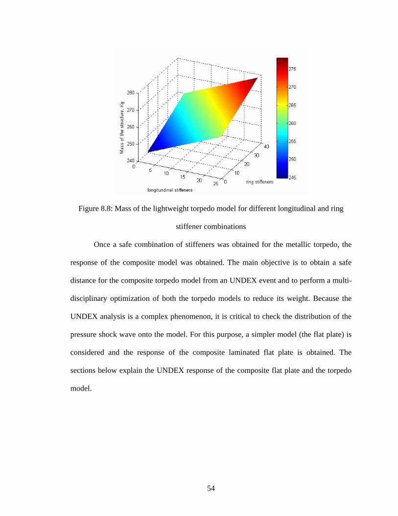
Figure 8.8: Mass of the lightweight torpedo model for different longitudinal and ring

stiffener combinations

Once a safe combination of stiffeners was obtained for the metallic torpedo, the

response of the composite model was obtained. The main objective is to obtain a safe

distance for the composite torpedo model from an UNDEX event and to perform a multi-

disciplinary optimization of both the torpedo models to reduce its weight. Because the

UNDEX analysis is a complex phenomenon, it is critical to check the distribution of the

pressure shock wave onto the model. For this purpose, a simpler model (the flat plate) is

considered and the response of the composite laminated flat plate is obtained. The

sections below explain the UNDEX response of the composite flat plate and the torpedo

model.

54

8.4 Composite Flat Plate Response

A flat plate that has the same length as the torpedo model was analyzed in this research.

The stacking sequence, thickness of each layer, thickness of the honeycomb, and the

material properties of the laminates and the honeycomb core are given the same as that of

the torpedo described in the chapter 2. The plate model was simply supported at the four

corners, and the loading was applied perpendicular to its surface. Since the plate is simply

supported at the ends and the shock wave hits the center of plate first and travels away

from the centre towards the ends, the bending deformation occurs along the length and

width of the plate. The maximum failure for the layers occurs at the corners of the plate,

which are pinned. As the standoff distance selected is closer (35 m) and the charge

weight higher (70 kg), the composite plate failed due to the UNDEX loading. However,

considering a simple structure such as a plate instead of a torpedo model enabled us to

look at the distribution of pressure on the structure and to obtain the layer- by-layer

response.

Figures 8.9 to 8.12 shows the distribution of the failure criterion values on

different layers in the composite. For a 0 and 90 degrees laminates, the maximum values

are cornered at the four ends as the fibers are placed in the directions along the length and

width of the plate, respectively. The 0o fibers resist the lengthwise bending of the plate,

which is similar to the effect that the longitudinal stiffeners had on the metallic structure.

The 90o fibers resist the widthwise bending of the plate which is similar to the effect that

the ring stiffeners have on the metallic structure. Since the composite materials are much

stronger in the fiber direction (0o) than in the direction perpendicular to the fiber (90o),

the 90o layer (even though they are not in direct contact with the shock wave as is the 0o

55

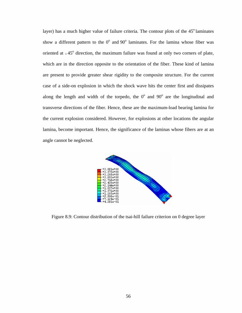
layer) has a much higher value of failure criteria. The contour plots of the 45o laminates

show a different pattern to the 0o and 90o laminates. For the lamina whose fiber was

oriented at ± 45o direction, the maximum failure was found at only two corners of plate,

which are in the direction opposite to the orientation of the fiber. These kind of lamina

are present to provide greater shear rigidity to the composite structure. For the current

case of a side-on explosion in which the shock wave hits the center first and dissipates

along the length and width of the torpedo, the 0o and 90o are the longitudinal and

transverse directions of the fiber. Hence, these are the maximum-load bearing lamina for

the current explosion considered. However, for explosions at other locations the angular

lamina, become important. Hence, the significance of the laminas whose fibers are at an

angle cannot be neglected.

Figure 8.9: Contour distribution of the tsai-hill failure criterion on 0 degree layer

56

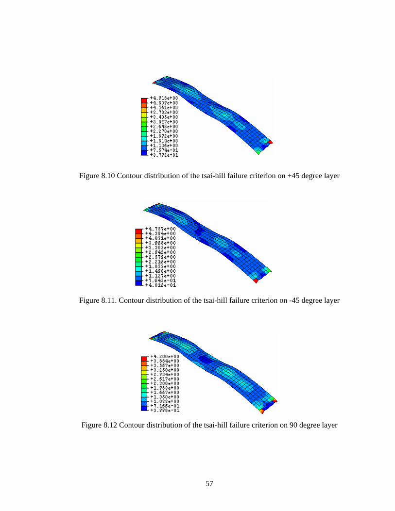
Figure 8.10 Contour distribution of the tsai-hill failure criterion on +45 degree layer

Figure 8.11. Contour distribution of the tsai-hill failure criterion on -45 degree layer

Figure 8.12 Contour distribution of the tsai-hill failure criterion on 90 degree layer

57

8.5 Composite Lightweight Torpedo Response

Once the response of the flat plate is obtained and the effect and importance of the

different layers is studied, the response of the lightweight torpedo model is obtained. In

this paper, the UNDEX analysis of the lightweight torpedo was conducted at different

stand-off distances and for different charge weights using the similitude relations. The

standoff distances and charge weights considered are 5, 10, 15, 20,….70 m and 5,10, 15,

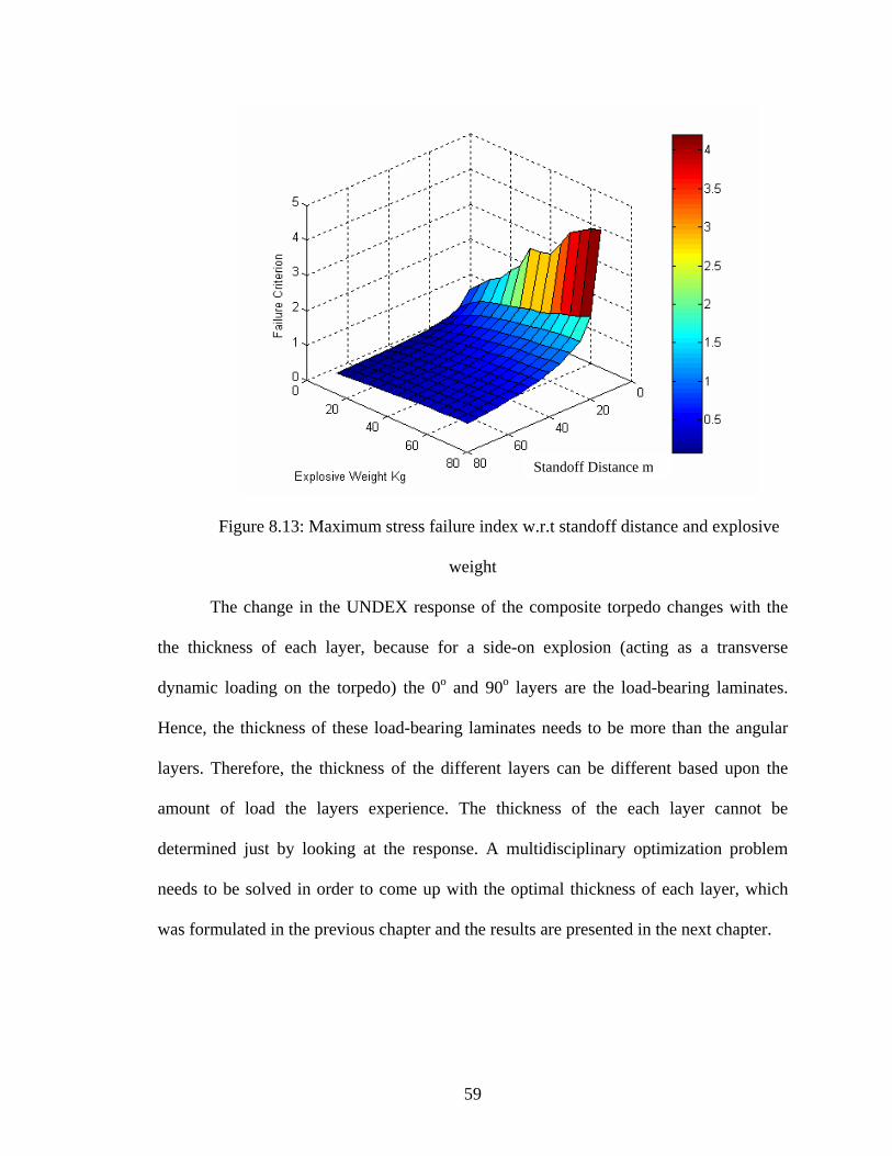
20,….70 kg, respectively. The 3-D plot in Figure 8.13 shows the maximum failure

criteria of the composite structure produced due to a certain charge at a certain stand-off

distance. From the surface of the plot we can see that as the standoff distance is increased,

the value of the failure criterion decreases. Similarly, as the charge weight increases, the

value of the failure criterion increases as expected. From the plot we can say that for a 70

kg of HBX-1 charge the safe distance is between 30 to 25m and the critical distance is 25

to 20 m. The figure clearly shows that the response of the composite torpedo is more

sensitive to the standoff distance than the explosive weight. These results are in

accordance with Ref [18], in which a similar kind of behavior was obtained, where the

displacement of the structure was considered with respect to standoff distance and the

charge weight. In this case too, it is observed that decreasing the stand-off distance has

more effect than increasing the charge weight.

58

Standoff Distance m

Figure 8.13: Maximum stress failure index w.r.t standoff distance and explosive

weight

The change in the UNDEX response of the composite torpedo changes with the

the thickness of each layer, because for a side-on explosion (acting as a transverse

dynamic loading on the torpedo) the 0o and 90o layers are the load-bearing laminates.

Hence, the thickness of these load-bearing laminates needs to be more than the angular

layers. Therefore, the thickness of the different layers can be different based upon the

amount of load the layers experience. The thickness of the each layer cannot be

determined just by looking at the response. A multidisciplinary optimization problem

needs to be solved in order to come up with the optimal thickness of each layer, which

was formulated in the previous chapter and the results are presented in the next chapter.

59

9. Optimization Results

The optimization results are obtained for both torpedo models at their critical

distances. The critical distance for the composite and metallic torpedoes are obtained at

20 m and 35 m, respectively. Furthermore, the comparison of the optimal results for both

models is made at a standoff distance of 35 m.

9.1 Composite Lightweight Torpedo

The optimization problem is solved to obtain the torpedo design with the least

weight that is safe at 20 m and 35 m standoff distances for a 70 kg HBX-1 charge. The

results of the optimization can be seen in Tables 9.1 and 9.2. The weight of the model is

228.77 kg for a 20 m standoff distance, as observed in the response. The 0o and 90o layers

are the maximum load-bearing laminates; hence, they are of the maximum thickness,

apart from the honeycomb. The +45o and -45o laminates that support the composite

model in shear have a thickness of 0.2 mm and 0.3 mm, respectively. The honeycomb

placed at the center increases the strength and rigidity of the structure with a very low

increase in weight. As we can observe from Tables 9.1 and 9.2, the thickness of the

honeycomb is more than all of the layers, but its contribution to the weight of the

structure is disproportionately low.

60

228.77

Mass (kg)

Objective

0.922.114.01.50.30.21.5

UNDEXFrequency (Hz)

Honey-comb

90o-45o+45o0o

ConstraintsDesign VariablesThicknesses, mm

228.77

Mass (kg)

Objective

0.922.114.01.50.30.21.5

UNDEXFrequency (Hz)

Honey-comb

90o-45o+45o0o

ConstraintsDesign VariablesThicknesses, mm

Table 9.1: Optimized results for the composite lightweight torpedo at 20 m standoff

distance

222.65

Mass (kg)

Objective

0.922.08.70.30.10.12.1

UNDEXFrequency (Hz)

Honey-comb

90o-45o+45o0o

ConstraintsDesign VariablesThicknesses, mm

222.65

Mass (kg)

Objective

0.922.08.70.30.10.12.1

UNDEXFrequency (Hz)

Honey-comb

90o-45o+45o0o

ConstraintsDesign VariablesThicknesses, mm

Table 9.2: Optimized results for the composite lightweight torpedo at 35 m standoff

distance

9.2 Metallic Lightweight Torpedo

For the case of the metallic torpedo, the optimization was performed at a standoff

distance of 35m for a 70 kg HBX-1 charge. This standoff distance was chosen because it

was the critical distance at which an unstiffened lightweight torpedo failed, as predicted

in the above section. Table 9.3 shows the optimized results for the 7&8, 8&8, and 14&8

ring and longitudinal stiffener combinations. From the table we can observe that the least

weight design is the torpedo with 8 ring and 8 longitudinal stiffeners.

61

254.52

251.69

251.27

Initial torpedo

mass, kg

247.547 ring & 12 long

247.368 ring & 8 long

247.947 ring & 8 long

Optimum torpedo

mass, kg

Stiffener combination

247.547 ring & 12 long

247.368 ring & 8 long

247.947 ring & 8 long

Optimum torpedo

mass, kg

Stiffener combination

254.52

251.69

251.27

Initial torpedo

mass, kg

Table 9.3: Optimized results for the metallic lightweight torpedo at 35 m standoff

distance for 3 different stiffener combinations

Also, the surface in Figure 9.1 shows the optimum weight values obtained for

different combinations of ring and longitudinal stiffeners. We can observe that the plot

varies nonlinearly and we can pick the least weight design from the plot. The response of

the torpedo to UNDEX also depends on the positions of the stiffeners and the position of

the explosive. The optimized results presented in this research are for a certain placement

of the stiffeners and for a side-on explosion.

62

Figure 9.1: Optimum weight value with respect to ring and longitudinal stiffener

combination

When the optimization results of both torpedo models are compared at a standoff

distance of 35 m, it can be observed that the weight of the composite model is 25 kg less

than that of the metallic model. The reduction in weight is obtained due to the lower

weight of the composite shell that comprises the honeycomb and the different lamina

whose weight are less than the aluminum shell of the metallic model of the torpedo.

63

10. Conclusions and Future work

10.1 Conclusions

A torpedo configurational design was performed to determine the lightest and

safest structure to satisfy the blast response criterion. In order to avoid complex and

expensive physical testing to determine the structural response to an underwater

explosion, a numerical technique was explored. This technique integrated the fluid and

structural behavior and solved a transient fluid-structure interaction problem. A

conventional unstiffened torpedo was analyzed to determine its response to an explosion

and to compare it with a stiffened torpedo. Various configurations of the torpedo were

explored where the stiffener position and the explosion position was altered. This study

accounts for all explosions due to a fixed amount of charge in the vicinity of the torpedo,

except the one right along the path of the torpedo. The safe distance obtained from this

research is used as one of the constraints in performing the multidisciplinary optimization

of the lightweight torpedo model. Along with the weight and stress constraints,

robustness of the selected design was also explored.

Also, an optimization problem is formulated and solved to obtain the least weight

design of a torpedo model when subjected to an UNDEX. A stiffened lightweight

metallic torpedo and a composite torpedo were designed. The composite structure was

modeled as a quasi-isotropic symmetric laminate. The UNDEX response of a laminated

64

flat plate was obtained by taking into consideration the fluid structure interaction effect.

The safe distance of a composite lightweight torpedo was obtained.

The optimized results of the composite and the metallic model are compared. It is

observed that the composite model was lighter and safer than the stiffened metallic

torpedo.

10.2 Future work

The current UNDEX response capability can be utilized in developing the next

generation torpedoes and unmanned undersea vehicles (UUV). By developing an acoustic

based or pressure based UNDEX sensing system that would aid in keeping the structure

at safe distance from the UNDEX shock wave the undersea vehicles resistance to

UNDEX can be increased. A control system can be developed which updates the

guidance and control section each time the vehicle encounters an UNDEX scenario. A

description of the formulation of problem for the development of the sensing system is

given below.

Control System:

The control system functions based upon the path optimization formulation. A

pressure transducer senses the pressure produced due to the shock wave. The response of

the torpedo due to UNDEX is achieved by applying the attained pressure onto the

structure. The control system will drive the torpedo away from the path of explosion and

thereby making it safe from the continuous counter attack from the enemy submarine.

65

Path Optimization:

A reliability based optimization problem is formulated in order for torpedo to

maintain a safe distance from the explosion. The problem formulation is given below

Objective:

Maximize (Probability of Kill)

Constraints:

a. Maximum Stress due to UNDEX <= Limit Value

b. Amount of fuel consumed < Total amount of fuel

Design Variables:

Stand-off distance between torpedo and explosion.

The above formulation would enable the torpedo to follow a path towards its

target which is the minimum safest distance. By placing the constraints on the fuel it is

ensured that the torpedo reaches its target before the fuel is consumed. The UNDEX

shock response is obtained by sensing the pressure produced due to the explosion.

Pressure transducers in the control system are used to obtain the total pressure of the

shock wave.

These formulations could make use of the current UNDEX analysis performed in

this research as a routine to determine whether the structure is safe or unsafe and thereby

maneuver the undersea vehicle in the specific direction. This enhancement in the

technology through the development of a control system would immensely increase the

structural safety of the torpedoes and other undersea vehicles in UNDEX scenarios

during real-time warfare.

66

APPENDIX

Appendix A

Radiation Boundary Condition

Many of the acoustic studies such as the UNDEX response involve a vibrating structure

in an infinite domain. In such cases we model a layer of the acoustic medium using finite

elements, to a thick ness of 1/3 to a full wavelength, out to a “radiating” boundary surface.

We then impose a condition on this surface to allow the acoustic waves to pass through

and not reflect back into the computational domain. For radiation boundaries of simple

shapes such as planes, spheres etc. simple impedance boundary conditions can represent

good approximations to the exact conditions.

In ABAQUS we apply the radiation boundary condition by specifying the

corresponding impedance, given as

)11()(11

pa

pc

xT += &

where T(x) is the boundary traction term ).1.()(xpnxT

f ∂∂

= −

ρ on the boundary surface.

1

1c

and 1

1a

are the admittance parameters which are defined as

67

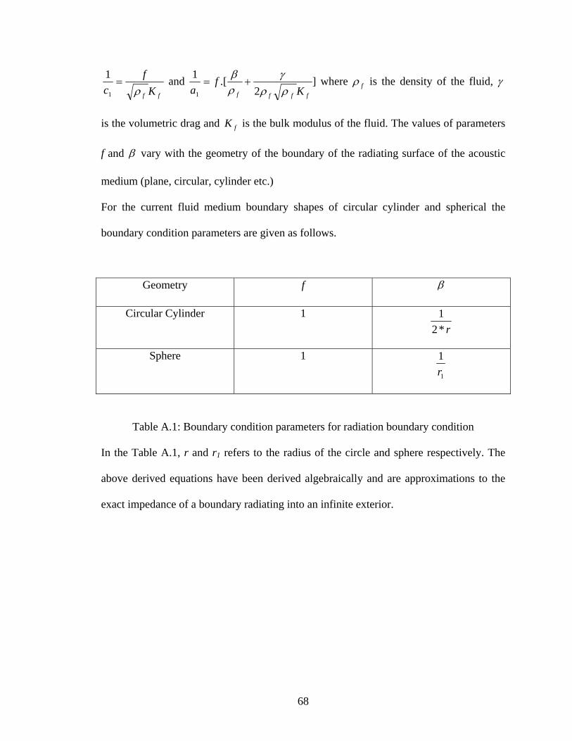
ff Kf

c ρ=

1

1 and ]2

.[1

1 ffff Kf

a ρργ

ρβ

+= where fρ is the density of the fluid, γ

is the volumetric drag and is the bulk modulus of the fluid. The values of parameters

f and

fK

β vary with the geometry of the boundary of the radiating surface of the acoustic

medium (plane, circular, cylinder etc.)

For the current fluid medium boundary shapes of circular cylinder and spherical the

boundary condition parameters are given as follows.

Geometry f β

Circular Cylinder 1 r*2

1

Sphere 1

1

1r

Table A.1: Boundary condition parameters for radiation boundary condition

In the Table A.1, r and r1 refers to the radius of the circle and sphere respectively. The

above derived equations have been derived algebraically and are approximations to the

exact impedance of a boundary radiating into an infinite exterior.

68

Appendix B

The code below is the input file in ABAQUS to perform an UNDEX response.

% Main input file in ABAQUS to obtain the UNDEX response *PART, NAME=WATER % Fluid nodes and element file *INCLUDE, INPUT = newwatsideloadnegy.inp *END PART %Structure nodes and element file *INCLUDE, INPUT = realtorpedo.inp %Assembling the Structure and the Fluid *ASSEMBLY, NAME=UNDEX *INSTANCE, NAME=WATER-1, PART=WATER 0., 0., 0. *END INSTANCE *INSTANCE, NAME=TORPEDO-1, PART=TORPEDO 0., 0., 0. *END INSTANCE %Defining the Surfaces for FSI and Radiation Boundary Condition *SURFACE, TYPE=ELEMENT, NAME=TORPEDO-FSI, NO THICK TORPEDO-1.ALLTORPEDOSHELL4ELEMENTS, SPOS *SURFACE, TYPE=ELEMENT, NAME=TORPEDO-LOAD, NO THICK TORPEDO-1.ALLTORPEDOLOADELEMENTS, SPOS *Surface, type=ELEMENT, name=CYL-BOUND-MID WATER-1.__PickedSurf4_S3, S3 WATER-1.__PickedSurf4_S2, S2 WATER-1.__PickedSurf4_S4, S4 WATER-1.__PickedSurf4_S1, S1 *Surface, type=ELEMENT, name=SPH-BOUND-LR WATER-1.__PickedSurf5_S3, S3 WATER-1.__PickedSurf5_S2, S2 WATER-1.__PickedSurf5_S4, S4 WATER-1.__PickedSurf5_S1, S1 *Surface, type=ELEMENT, name=WATER-FSI WATER-1.__PickedSurf6_S3, S3 WATER-1.__PickedSurf6_S2, S2 WATER-1.__PickedSurf6_S4, S4 WATER-1.__PickedSurf6_S1, S1 *Surface, type=ELEMENT, name=WATER-LOAD WATER-1.__PickedSurf19_S3, S3 WATER-1.__PickedSurf19_S4, S4 WATER-1.__PickedSurf19_S2, S2 WATER-1.__PickedSurf19_S1, S1 %Fluid-Structure interaction *TIE, NAME=FSI,ADJUST=YES, NO ROTATION

69

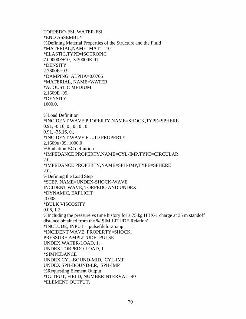
TORPEDO-FSI, WATER-FSI *END ASSEMBLY %Defining Material Properties of the Structure and the Fluid *MATERIAL,NAME=MAT1 101 *ELASTIC,TYPE=ISOTROPIC 7.00000E+10, 3.30000E-01 *DENSITY 2.7800E+03, *DAMPING, ALPHA=0.0705 *MATERIAL, NAME=WATER *ACOUSTIC MEDIUM 2.1609E+09, *DENSITY 1000.0, %Load Definition *INCIDENT WAVE PROPERTY,NAME=SHOCK,TYPE=SPHERE 0.91, -0.16, 0., 0., 0., 0. 0.91, -35.16, 0., *INCIDENT WAVE FLUID PROPERTY 2.1609e+09, 1000.0 %Radiation BC definition *IMPEDANCE PROPERTY,NAME=CYL-IMP,TYPE=CIRCULAR 2.0, *IMPEDANCE PROPERTY,NAME=SPH-IMP,TYPE=SPHERE 2.0, %Defining the Load Step *STEP, NAME=UNDEX-SHOCK-WAVE INCIDENT WAVE, TORPEDO AND UNDEX *DYNAMIC, EXPLICIT ,0.008 *BULK VISCOSITY 0.06, 1.2 %Including the pressure vs time history for a 75 kg HBX-1 charge at 35 m standoff distance obtained from the %‘SIMILITUDE Relation’ *INCLUDE, INPUT = pulsefilefor35.inp *INCIDENT WAVE, PROPERTY=SHOCK, PRESSURE AMPLITUDE=PULSE UNDEX.WATER-LOAD, 1. UNDEX.TORPEDO-LOAD, 1. *SIMPEDANCE UNDEX.CYL-BOUND-MID, CYL-IMP UNDEX.SPH-BOUND-LR, SPH-IMP %Requesting Element Output *OUTPUT, FIELD, NUMBERINTERVAL=40 *ELEMENT OUTPUT,

70

ELSET=UNDEX.TORPEDO-1.ALLTORPEDOSHELL4ELEMENTS S, MISES *END STEP

71

Appendix C

The C++ code below generates the ABAQUS input file for the structural model of the

lightweight torpedo

#include<iostream.h> #include<stdlib.h> #include<stdio.h> #include<math.h> void main() { char outfile[50]="abqcomptorpforstress.inp"; int j=0,k=0; FILE *stream2; stream2=fopen(outfile,"w"); //Part defenition fprintf(stream2,"%s\n","*Heading\n LIGHT WEIGHT TORPEDO"); fprintf(stream2,"%s\n","** PARTS"); fprintf(stream2,"%s\n","*Part, name=TORPEDO"); fprintf(stream2,"%s\n","*End Part"); fprintf(stream2,"%s\n","** ASSEMBLY"); fprintf(stream2,"%s\n","*Assembly,name=torpedo1"); fprintf(stream2,"%s\n","*Instance, name=torpedo-1, part=torpedo"); fprintf(stream2,"%s\n","LOADCASE 2"); fprintf(stream2,"%s\n","METHOD = 15"); int n_x, n_y,n_t, n_r, x,y,r, N1; double Dia, Len, Nose, th, xc,ti,h,ofs; Dia=0.32; //Diameter of body Len=2.0; //Length of body Nose=0.16; //Length of nose n_x=40; //Number of nodal rings on main body n_y=3; //Number of nodal rings on nose n_t=7; //Number of nodal rings on tail n_r=24; //Number of nodes on each ring ti=0.00635; //Thickness of shell h=0.010; //Height of stiffeners ofs=(ti/2)+(h/2); //offset for stiffners double GridCoordX[10000],GridCoordY[10000],GridCoordZ[10000], theta, X_coord; theta=360.0/24.0; N1=0; X_coord=2.00/40.0;

72

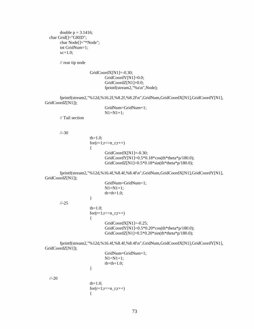
double p = 3.1416; char Grid[]="GRID"; char Node[]="*Node"; int GridNum=1; xc=1.0; // rear tip node GridCoordX[N1]=-0.30; GridCoordY[N1]=0.0; GridCoordZ[N1]=0.0; fprintf(stream2,"%s\n",Node); fprintf(stream2,"%12d,%16.2f,%8.2f,%8.2f\n",GridNum,GridCoordX[N1],GridCoordY[N1],GridCoordZ[N1]); GridNum=GridNum+1; N1=N1+1; // Tail section //-30 th=1.0; for(r=1;r<=n_r;r++) { GridCoordX[N1]=-0.30; GridCoordY[N1]=0.5*0.18*cos(th*theta*p/180.0); GridCoordZ[N1]=0.5*0.18*sin(th*theta*p/180.0); fprintf(stream2,"%12d,%16.4f,%8.4f,%8.4f\n",GridNum,GridCoordX[N1],GridCoordY[N1],GridCoordZ[N1]); GridNum=GridNum+1; N1=N1+1; th=th+1.0; } //-25 th=1.0; for(r=1;r<=n_r;r++) { GridCoordX[N1]=-0.25; GridCoordY[N1]=0.5*0.20*cos(th*theta*p/180.0); GridCoordZ[N1]=0.5*0.20*sin(th*theta*p/180.0); fprintf(stream2,"%12d,%16.4f,%8.4f,%8.4f\n",GridNum,GridCoordX[N1],GridCoordY[N1],GridCoordZ[N1]); GridNum=GridNum+1; N1=N1+1; th=th+1.0; } //-20 th=1.0; for(r=1;r<=n_r;r++) {

73

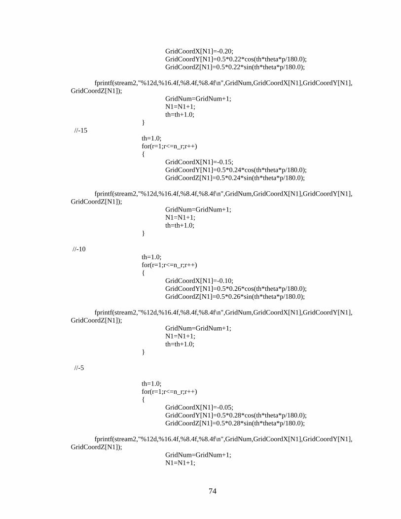
GridCoordX[N1]=-0.20; GridCoordY[N1]=0.5*0.22*cos(th*theta*p/180.0); GridCoordZ[N1]=0.5*0.22*sin(th*theta*p/180.0); fprintf(stream2,"%12d,%16.4f,%8.4f,%8.4f\n",GridNum,GridCoordX[N1],GridCoordY[N1],GridCoordZ[N1]); GridNum=GridNum+1; N1=N1+1; th=th+1.0; } //-15 th=1.0; for(r=1;r<=n_r;r++) { GridCoordX[N1]=-0.15; GridCoordY[N1]=0.5*0.24*cos(th*theta*p/180.0); GridCoordZ[N1]=0.5*0.24*sin(th*theta*p/180.0); fprintf(stream2,"%12d,%16.4f,%8.4f,%8.4f\n",GridNum,GridCoordX[N1],GridCoordY[N1],GridCoordZ[N1]); GridNum=GridNum+1; N1=N1+1; th=th+1.0; } //-10 th=1.0; for(r=1;r<=n_r;r++) { GridCoordX[N1]=-0.10; GridCoordY[N1]=0.5*0.26*cos(th*theta*p/180.0); GridCoordZ[N1]=0.5*0.26*sin(th*theta*p/180.0); fprintf(stream2,"%12d,%16.4f,%8.4f,%8.4f\n",GridNum,GridCoordX[N1],GridCoordY[N1],GridCoordZ[N1]); GridNum=GridNum+1; N1=N1+1; th=th+1.0; } //-5 th=1.0; for(r=1;r<=n_r;r++) { GridCoordX[N1]=-0.05; GridCoordY[N1]=0.5*0.28*cos(th*theta*p/180.0); GridCoordZ[N1]=0.5*0.28*sin(th*theta*p/180.0); fprintf(stream2,"%12d,%16.4f,%8.4f,%8.4f\n",GridNum,GridCoordX[N1],GridCoordY[N1],GridCoordZ[N1]); GridNum=GridNum+1; N1=N1+1;

74

th=th+1.0; } //0 th=1.0; for(r=1;r<=n_r;r++) { GridCoordX[N1]=0; GridCoordY[N1]=0.5*0.30*cos(th*theta*p/180.0); GridCoordZ[N1]=0.5*0.30*sin(th*theta*p/180.0); fprintf(stream2,"%12d,%16.4f,%8.4f,%8.4f\n",GridNum,GridCoordX[N1],GridCoordY[N1],GridCoordZ[N1]); GridNum=GridNum+1; N1=N1+1; th=th+1.0; } // Main body for(x=1;x<=n_x;x++) { th=1.0; for(r=1;r<=n_r;r++) { GridCoordX[N1]=xc*X_coord; GridCoordY[N1]=0.5*Dia*cos(th*theta*p/180.0); GridCoordZ[N1]=0.5*Dia*sin(th*theta*p/180.0); fprintf(stream2,"%12d,%16.4f,%8.4f,%8.4f\n",GridNum,GridCoordX[N1],GridCoordY[N1],GridCoordZ[N1]); GridNum=GridNum+1; N1=N1+1; th=th+1.0; } xc=xc+1.0; } // Nose section X_coord=0.16/4.0; xc=1.0; for(y=1;y<=n_y;y++) { th=1.0; for(r=1;r<=n_r;r++) { GridCoordX[N1]=xc*X_coord+2.0; GridCoordY[N1]=0.5*Dia*0.25*(4.0-xc)*cos(th*theta*p/180.0); GridCoordZ[N1]=0.5*Dia*0.25*(4.0-xc)*sin(th*theta*p/180.0); fprintf(stream2,"%12d,%16.4f,%8.4f,%8.4f\n",GridNum,GridCoordX[N1],GridCoordY[N1],GridCoordZ[N1]); GridNum=GridNum+1; N1=N1+1; th=th+1.0; }

75

xc=xc+1.0; } // Tip Node GridCoordX[N1]=Len+0.12; GridCoordY[N1]=0.0; GridCoordZ[N1]=0.0; fprintf(stream2,"%12d,%16.4f,%8.4f,%8.4f\n",GridNum,GridCoordX[N1],GridCoordY[N1],GridCoordZ[N1]); GridNum=GridNum+1; N1=N1+1; int ElmNum=1; char ELEM[]="*Element, type=S4R"; char ELEM1[]="*Element, type=S3R"; char plus[]="+"; j=2; // Rear tria3 elements fprintf(stream2,"%s\n",ELEM1); for(r=1;r<n_r;r++) { fprintf(stream2,"%12d,%8d,%8d,%8d\n",ElmNum,j,j+1,1); ElmNum=ElmNum+1; j=j+1; } fprintf(stream2,"%12d,%8d,%8d,%8d\n",ElmNum,j,j-n_r+1,1); ElmNum=ElmNum+1; int pq,pr; pr=n_x+n_y+n_t; pq=(n_x+n_y+n_t)/3; fprintf(stream2,"%s\n",ELEM); j=2; for(x=1;x<pq;x++) { for(r=1;r<n_r;r++) { fprintf(stream2,"%10d,%8d,%8d,%8d,%8d\n",ElmNum,j,j+1,j+n_r+1,j+n_r); ElmNum=ElmNum+1; j=j+1; } fprintf(stream2,"%10d,%8d,%8d,%8d,%8d\n",ElmNum,j,j-n_r+1,j+1,j+n_r); ElmNum=ElmNum+1; j=j+1; } for(x=pq;x<2*pq;x++) {

76

for(r=1;r<n_r;r++) { fprintf(stream2,"%10d,%8d,%8d,%8d,%8d\n",ElmNum,j,j+1,j+n_r+1,j+n_r); ElmNum=ElmNum+1; j=j+1; } fprintf(stream2,"%10d,%8d,%8d,%8d,%8d\n",ElmNum,j,j-n_r+1,j+1,j+n_r); ElmNum=ElmNum+1; j=j+1; } for(x=2*pq;x<pr;x++) { for(r=1;r<n_r;r++) { fprintf(stream2,"%10d,%8d,%8d,%8d,%8d\n",ElmNum,j,j+1,j+n_r+1,j+n_r); ElmNum=ElmNum+1; j=j+1; } fprintf(stream2,"%10d,%8d,%8d,%8d,%8d,\n",ElmNum,j,j-n_r+1,j+1,j+n_r); ElmNum=ElmNum+1; j=j+1; } //Nose tip elements fprintf(stream2,"%s\n",ELEM1); for(r=1;r<n_r;r++) { fprintf(stream2,"%10d,%8d,%8d,%8d\n",ElmNum,j,j+1,1202); ElmNum=ElmNum+1; j=j+1; } fprintf(stream2,"%10d,%8d,%8d,%8d\n",ElmNum,j,j-n_r+1,1202); ElmNum=ElmNum+1; //Ribs char ELEM2[]="*ELEMENT, TYPE=B31, ELSET=BARELEMENTS"; j=194;//281 float a,b,c,m,d,e,f; float p1,q,r1,m1,s,t,u; float X=0.10; float Y=0; float Z=0; fprintf(stream2,"%s\n",ELEM2); for(x=1;x<n_x;) { for(r=1;r<n_r;r++)

77

{ a=GridCoordX[j-1]-X; b=GridCoordY[j-1]-Y; c=GridCoordZ[j-1]-Z; // m=sqrt(a*a+b*b+c*c); // d=-ofs*a/m; // e=-ofs*b/m; // f=-ofs*c/m; p1=GridCoordX[j]-X; q=GridCoordY[j]-Y; r1=GridCoordZ[j]-Z; // m1=sqrt(p1*p1+q*q+r1*r1); // s=-ofs*p1/m1; // t=-ofs*q/m1; // u=-ofs*r1/m1; fprintf(stream2,"%12d,%8d,%8d\n",ElmNum,j,j+1); ElmNum=ElmNum+1; j=j+1; } a=GridCoordX[j-1]-X; b=GridCoordY[j-1]-Y; c=GridCoordZ[j-1]-Z; // m=sqrt(a*a+b*b+c*c); // e=-ofs*b/m; // f=-ofs*c/m; p1=GridCoordX[j-n_r]-X; q=GridCoordY[j-n_r]-Y; r1=GridCoordZ[j-n_r]-Z; // m1=sqrt(p1*p1+q*q+r1*r1); // s=-ofs*p1/m1; // t=-ofs*q/m1; // u=-ofs*r1/m1; fprintf(stream2,"%12d,%8d,%8d\n",ElmNum,j,j-n_r+1); ElmNum=ElmNum+1; j=j+49;//49; x=x+3.0;//3 X=X+0.15;//15 // a1=a1+1; } // longitudinal bars double J[10]; int i;

78

J[0]=196.0; J[1]=199.0; J[2]=202.0; J[3]=205.0; J[4]=208.0; J[5]=211.0; J[6]=214.0; J[7]=217.0; Y=0; Z=0; for (i=0;i<8;i++) { j=J[i]; X=0.10; for (x=1;x<(n_x)-1;x++) { k=j+24; a=GridCoordX[j-1]-X; b=GridCoordY[j-1]-Y; c=GridCoordZ[j-1]-Z; // m=sqrt(a*a+b*b+c*c); // d=-ofs*a/m; // e=-ofs*b/m; // f=-ofs*c/m; X=X+0.05; p1=GridCoordX[k-1]-X; q=GridCoordY[k-1]-Y; r1=GridCoordZ[k-1]-Z; // m1=sqrt(p1*p1+q*q+r1*r1); // s=-ofs*p1/m1; // t=-ofs*q/m1; // u=-ofs*r1/m1; fprintf(stream2,"%12d,%8d,%8d\n",ElmNum,j,k); ElmNum=ElmNum+1; j=j+24; } } */ //abaqus mass elements double C[10]; C[0]=0.45; C[1]=1.25; C[2]=1.95; int g,G,pid,lp,N; double NR; NR=0.10; G=196;

79

pid=1; N=1; //char Node1[]="*Nset"; char Element1[]="*Element"; char Mass[]="*Mass"; fprintf(stream2,"%s,%s,%s\n",Node1,"nset=PT-MASS","generate"); fprintf(stream2,"%d,%d,%d\n",196,361,3); fprintf(stream2,"%d,%d,%d\n",412,721,3); fprintf(stream2,"%d,%d,%d\n",772,1009,3); fprintf(stream2,"%d,%d,%d\n",1060,1081,3); fprintf(stream2,"%s,%s,%s%d\n",Element1,"Type=MASS","Elset=PT-MASS",pid); for (g=0;g<3;g++) { while(NR<C[g]) { for(lp=1;lp<=8;lp++) { fprintf(stream2,"%11d,%8d\n",ElmNum,G); ElmNum=ElmNum+1; G=G+3; } NR=NR+0.15; G=G+48; } } fprintf(stream2,"%s,%s%d\n",Mass,"Elset=PT-MASS",pid); fprintf(stream2,"%16.4f\n",1.9231); int el,mp; int intergrid[200]; el=0; j=196; for (x=1;x<=49;x++) { for (lp=1;lp<=8;lp++) { intergrid[el]=j; j=j+3; el=el+1; } j=j+48; el=el+1; x=x+3; } for (mp=0;mp<130;mp++) { printf("%d\n",intergrid[mp]); }

80

// Property definition // fprintf(stream2,"%s,%s,%s\n","*BEAM GENERAL SECTION","ELSET=BARELEMENTS","DENSITY=2823.0"); // fprintf(stream2,"%s,%s,%s,%s,%s,%s,%s\n\n","0.15E-3","0.28125E-8","0.0","0.125E-8","0.29346E-8","0","0.0"); // fprintf(stream2,"%s,%s,%s\n","0.7E+11","0.26316E+11","0.00"); //fprintf(stream2,"%s%10d%8d%8.5f%8d\n","PSHELL",1,101,ti,101); //fprintf(stream2,"%s%10d%8d%8.5f%8d\n","PSHELL",4,102,ti,102); //******************************************************************** //***************FOR COMPOSITES****************** fprintf(stream2,"%s%\n%s\n","*NSET, NSET=NODE1","1"); fprintf(stream2,"%s%\n%s\n","*NSET, NSET=NODE2, GENERATE","2, 25, 1"); fprintf(stream2,"%s%\n%s\n","*NSET, NSET=NODE3","175, 187"); fprintf(stream2,"%s%\n%s\n","*NSET, NSET=NODE4","181, 193"); fprintf(stream2,"%s%\n%s\n","*NSET, NSET=ALLTORPEDONODES, GENERATE","1, 1215, 1"); fprintf(stream2,"%s%\n%s\n","*ELSET, ELSET=ALLTORPEDOSHELL4ELEMENTS, generate","1, 1224, 1"); //************************************************************ fprintf(stream2,"%s%\n%s\n%s\n%s\n%s\n%s\n%s\n%s\n%s\n%s\n%s\n%s\n%s\n%s\n","*ELSET, ELSET=ALLTORPEDOLOADELEMENTS, generate","36, 1116, 24","37, 1117, 24","38, 1118, 24","39, 1119, 24","40, 1120, 24","41, 1121, 24","42, 1122, 24","43, 1123, 24","44, 1124, 24","45, 1125, 24","46, 1126, 24","47, 1127, 24"); fprintf(stream2,"%s\n%8.6f, %8.6f\n","*BEAM SECTION, ELSET=BARELEMENTS, MATERIAL=MAT, SECTION=RECT",0.015, 0.01); // Material properties //*********************************************************************** fprintf(stream2,"%s\n","*MATERIAL, NAME=FIBER"); fprintf(stream2,"%s\n","*ELASTIC, TYPE=LAMINA"); fprintf(stream2,"%s\n","1.4E+11,9.0E+9,0.30,7.1E+9,7.1E+9,7.1E+9"); fprintf(stream2,"%s\n","*DENSITY"); fprintf(stream2,"%s\n","1600.0,"); fprintf(stream2,"%s\n","*MATERIAL, NAME=COMB"); fprintf(stream2,"%s\n","*ELASTIC, TYPE=LAMINA"); fprintf(stream2,"%s\n","1.0E+0,1.0E+0,0.30,1.0E+0,1.1E+8,5.5E+ 7"); // Boundary Conditions fprintf(stream2,"%s\n","*Boundary"); fprintf(stream2,"%s\n","node1, 1, 1"); fprintf(stream2,"%s\n","node1, 2, 2"); fprintf(stream2,"%s\n","node1, 3, 3"); fprintf(stream2,"%s\n","node2, 1, 1"); fprintf(stream2,"%s\n","node3, 2, 2"); fprintf(stream2,"%s\n","node4, 3, 3"); // ****************************************** /*//Natural Frequency Analysis fprintf(stream2,"%s\n","*RESTART, WRITE"); fprintf(stream2,"%s\n","*Step"); fprintf(stream2,"%s\n","*Frequency, eigensolver=lanczos"); fprintf(stream2,"%s\n","21, , ,1000"); fprintf(stream2,"%s\n","*EL PRINT,FREQUENCY=0"); fprintf(stream2,"%s\n","*NODE PRINT, FREQUENCY=0"); fprintf(stream2,"%s\n","*MODAL FILE"); fprintf(stream2,"%s\n","*OUTPUT, FIELD, VARIABLE=PRESELECT");

81

fprintf(stream2,"%s\n","*MODAL OUTPUT"); fprintf(stream2,"%s\n","*END STEP");*/ //*************************************** fprintf(stream2,"%s\n","*End Part"); fprintf(stream2,"%s\n","*End Instance"); fprintf(stream2,"%s\n","*End Assembly"); fclose(stream2); }

82

Appendix D

The following FORTRAN code was used to perform the multi-disciplinary optimization

using the Design Optimization Tool (DOT).

DIMENSION X(20),XL(20),XU(20),G(200),

*WK(800),IWK(200),RPRM(20),IPRM(20) C DEFINE NRWK, NRIWK. NRWK=800 NRIWK=200 C ZERO RPRM AND IPRM. DO 10 I=1,20 RPRM(I)=0.0 10 IPRM(I)=0 C DEFINE METHOD,NDV,NCON. METHOD=1 C FOUR DESIGN VARIABLES. NDV=3 C CONSTRAINT NCON=2 C DEFINE BOUNDS AND INITIAL DESIGN. C INITIAL VALUES. X(1)=0.00628627 X(2)=0.013321 X(3)=0.00777577 C DO 20 I=1, NDV XL(1)=0.006 XU(1)=0.008 XL(2)=0.0001 XU(2)=0.1 XL(3)=0.0001 XU(3)=0.1 C C DEFINE IPRINT, MINMAX, INFO. C PRINT CONTROL. IPRINT=3 C MINIMIZE MINMAX=-1 C INITIALIZE INFO TO ZERO. INFO=0 C CALL EVAL(OBJ,X,BETA,B3,B4,G) C OPTIMIZE. 100 CALL DOT (INFO,METHOD,IPRINT,NDV,NCON,X,XL,XU, *OBJ,MINMAX,G,RPRM,IPRM,WK,NRWK,IWK,NRIWK) C FINISHED? IF(INFO.EQ.0)STOP C EVALUATE OBJECTIVE AND CONSTRAINT. CALL EVAL(OBJ,X,G) C GO CONTINUE WITH OPTIMIZATION. GO TO 100 END C C

83

SUBROUTINE EVAL (OBJ,X,G) C SUBROUTINE TO EVALUATE THE OBJECTIVE FUNCTION AND CONSTRAINTS DIMENSION X(*),G(*) CHARACTER *20 OUTFILE, OUT1, INPUT, INPUT1, INPUT2 CHARACTER *10 C OUTFILE="FforC.dat" OUT1="fforc.dat" OPEN(UNIT=11, FILE=OUTFILE, STATUS='UNKNOWN') OPEN(UNIT=12, FILE=OUT1, STATUS='UNKNOWN') WRITE(11, 2222) (X(I), I=1,3) WRITE(12, 2222) (X(I), I=1,3) CLOSE(11) C="runfrun" CALL SYSTEM(C) INPUT="mass.dat" OPEN(13, FILE=INPUT, STATUS='OLD') READ(13,*) OBJ INPUT1="freq.dat" OPEN(14, FILE=INPUT1, STATUS='OLD') READ(14,*) G(1) INPUT2="mise.dat" OPEN(15, FILE=INPUT2, STATUS='OLD') READ(15,*) G(2) CLOSE(13) CLOSE(14) CLOSE(15) 2222 FORMAT(F10.8) RETURN CLOSE(12) END

84

References

1) Rajendran, R., Narsimhan, K., “Linear Elastic Shock Response of Plane Plates

Subjected to Underwater Explosion,” International Journal of Impact

Engineering, Vol. 25, 2001, pp. 493-506.

2) Burch, I.A., and Mouritz, A.P., “Analysis of Responses of a Small Shock

Platform Subjected to Underwater Explosions,” DSTO Report, DSTO-TR-0891,

1999.

3) Rajendran, R., Narsimhan, K., “Damage Prediction of Clamped Circular Plates

Subjected to Contact Underwater Explosion,” International Journal of Impact

Engineering, Vol. 25, 2001, pp. 373-386.

4) Felippa, C.A., “Top-Down Derivation of Doubly Asymptotic Approximations for

Structure-Fluid Interaction Analysis,” Innovative Numerical Analysis for the

Engineering Sciences, University Press of Virginia, 1980, pp. 79-88.

5) Geers, T.L., “Doubly Asymptotic Approximations for Transient Motions of

Submerged Structures,” Journal of Acoustical Society of America, Vol. 64, 1978,

pp. 1500-1508.

6) Kwon, Y. W., and Cunningham, R. E., “Comparison of USA-Dyna Finite

Element Models for a Stiffened Shell Subject to Underwater Shock,” Computers

and Structures, Vol. 66, No. 1, 1998, pp 127-144.

85

7) Kwon, Y. W., and Fox, P. K., “Underwater Shock Response of a Cylinder

Subjected to a Side-on Explosion,” Computers and Structures, Vol. 48, No. 4,

1993, pp 637-646.

8) McCoy, R.W., Sun, C.T., “Fluid-Structure Interaction Analysis of a Thick Section

Composite Cylinder Subjected to Underwater Blast Loading,” Composite

Structures, Vol. 37, No. 1, 1997, pp 45-55.

9) Shin, Y.S., and Hooker,D.T, “Damage Response of Submerged Imperfect

Cylindrical Structures to Underwater Explosion,” Computers and Structures, Vol.

60, No. 5, 1996, pp. 683-693.

10) Arden, K.E., “Use of MSC/NASTRAN in Predicting Structural Response to an

Underwater Explosion,” MSC 1995 World Users' Conference Proceedings, Paper

No. 51, May, 1995.

11) Adamczyk, R., Cichocki, K., and Ruchwa, M., “Analysis of the Shock Response

of an Underwater Structure Subjected to a Far-Field Explosion,” Proceedings of

ABAQUS Users’ Conference, Milan, 1997, pp. 73-87.

12) Cichocki, K., “Computer Analysis of Dynamic Response due to Underwater

Explosion on Hybrid Structure,” Proceedings of ABAQUS Users’ Conference,

Newport, 1994, pp. 207-220.

13) Mouritz,A.P., Gellert,E., Burchhill,P., and K.Challis , “Review of advanced

composite structures for naval ships and submarines,” Composite Structures, vol.

53, 2001, pp. 21–41.

14) Mouritz, A.P., “The effect of underwater explosion shock loading on the fatigue

behaviour of GRP laminates,” Composites, vol. 26, 1995, pp.3–9.

86

15) Turkmen, H.S., and Mecitoglu, Z., “Dynamic response of a stiffened laminated

composite plate subjected to blast load,” Journal of Sound and Vibration, vol.

221, 1999, pp. 371-389.

16) Aslan, Z., Karakuzu, R., and Okutan, B., “The response of laminated composite

plates under low-velocity impact loading,” Composite Strucutres, vol. 59, 2003,

pp. 119-127.

17) Dyka, C.T., and Badaliance, R., “Damage in marine composites caused by shock

loading,” Composites Science and Technology, vol. 58, 1998, pp. 1433-1442.

18) Lam, K.Y, Zong, Z., and Wang, Q.X., “Dynamic response of a laminated pipeline

on the seabed subjected to underwater shock,” Composites Part B: engineering,

vol. 34, 2003, pp. 59-66.

19) Penmetsa, R. C., Grandhi, R. V., and Venkayya, V.B., “Modeling, Analysis, and

Uncertainty Quantification of a Lightweight Torpedo Design,” Journal of Naval

Engineers, Vol. 116, No. 4, 2004, pp. 23-36.

20) ABAQUS Theory Manual, Version 6.4.1. Hibbitt, Karlsson, and Sorensen, Inc.,

Pawtucket, RI, 2003.

21) Geers, T. L., Hunter, L. S., “An Integrated Wave-Effects Model for an

Underwater Explosion Bubble,” Journal of Acoustical Society of America, Vol.

111, No. 4, April 2002, pp 1584-1601.

22) Coles, R. H., Underwater Explosions, Princeton University Press, Princeton, 1948.

23) Gurdal, Z., Haftka, R.T., and Hajela, P., Design and optimization of laminated

composite material, John Wiley & Sons, inc., 1999, ch. 6.

87

24) Adduri, P., Penmetsa, R.C., and Grandhi, R.V., “Optimization of Lightweight

Composite Torpedo Structure with System Reliability Constraint,” Submitted to

Journal of Structural and Multidisciplinary Optimization, August 2005.

88