MULTIDISCIPLINARY FREE MATERIAL … FREE MATERIAL OPTIMIZATION J. HASLINGER , M. KOCVARAˇ y, G. LEUGERINGz, AND M. STINGLx Abstract. We present a mathematical framework for the so-called

MULTIDISCIPLINARY FREE MATERIAL OPTIMIZATION

J. HASLINGER∗, M. KOCVARA†, G. LEUGERING‡, AND M. STINGL§

Abstract. We present a mathematical framework for the so-called multidisciplinary free material optimization(MDFMO) problems, a branch of structural optimization in which the full material tensor is considered as a designvariable. We extend the original problem statement by a class of generic constraints depending either on the designor on the state variables. Among the examples are local stress or displacement constraints. We show the existenceof optimal solutions for this generalized FMO problem and discuss convergent approximation schemes based on thefinite element method.

Key words. structural optimization, material optimization, H-convergence, semidefinite programming, nonlin-ear programming

AMS subject classifications. 74B05, 74P05, 90C90, 90C30, 90C22

1. Introduction. Free material optimization (FMO) is a branch of structural optimiza-tion. The underlying FMO model was introduced in [4] and further studied in several paperssuch as, for example, [3, 23]. The design variable in FMO is represented by the full elasticstiffness tensor that can vary from point to point. The method is supported by powerful op-timization and numerical techniques which allow scenarios with complex bodies, fine finite-element meshes and many load cases. FMO has been successfully used for conceptual designof aircraft components; the most prominent example is the design of ribs in the leading edgeof Airbus A380 [11].

The basic FMO model has certain limitations, though. For example, structures may faildue to high stresses, or due to lack of stability (see [12, 13] for further discussion). In orderto prevent this undesirable behavior, additional requirements have to be taken into accountin the FMO model. Typically, such modifications lead to additional constraints on the set ofadmissible materials and/or the set of admissible displacements. These constraints usuallydestroy the favorable mathematical structure of the original problem (see [12, 13]).

As a consequence, the standard theorems ensuring the existence of optimal solutions andconvergence of appropriate approximation schemes fail to hold. In particular, it turns out thatin order to prove the existence of optimal solutions of the extended FMO problem, completelydifferent mathematical tools have to be applied. The tool used in our paper is the so-calledH-convergence introduced by Murat and Tartar [20, 15], a concept originally invented in thecontext of homogenized materials.

In the first part of the paper we briefly list the classic FMO results and discuss variousways of proving the existence of optimal solutions. We then formulate a class of multidis-ciplinary FMO problems (MDFMO) and use H-convergence in order to prove the existenceof optimal solutions under reasonable assumptions. Then, in Section 3, we propose an ap-proximation scheme for continuous setting of MDFMO problems, which is based on thediscretization of the design space by piecewise constant functions. We further prove that a

∗Department of Numerical Mathematics, Charles University, Sokolovska 83, 186 75 Praha 8, Czech Republic([email protected]).,†School of Mathematics, University of Birmingham, Birmingham B15 2TT, UK, and Institute of Information

Theory and Automation, Academy of Sciences of the Czech Republic, Pod vodarenskou vezı 4, 182 08 Praha 8,Czech Republic ([email protected])‡Department Mathematics, Applied Mathematics II, University of Erlangen, Martensstr. 3, 91058 Erlangen, Ger-

many ([email protected])§Department Mathematics, Applied Mathematics II, University of Erlangen, Martensstr. 3, 91058 Erlangen, Ger-

many ([email protected])

1

2 J. HASLINGER, M. KOCVARA, G. LEUGERING, AND M. STINGL

subsequence of optimal solutions of the discrete problems converges to a solution of the orig-inal problem in an appropriate sense. Finally, we discuss convergence of fully discretizedoptimization problems, and propose a discretization based on the finite element method.

Throughout this paper we use the following notation: We denote by SN the space of sym-metric N×N matrices equipped with the standard inner product 〈·, ·〉 defined by 〈A,B〉 :=Tr(AB) for any A,B ∈ SN , where Tr(C) denotes the trace of the matrix C ∈ SN . Wefurther denote by SN+ the cone of all positive semidefinite matrices in SN and use the abbre-viation A < 0 for matrices A ∈ SN+ . Moreover, for A,B ∈ SN , we say that A < B ifA−B < 0, and similarly for A 4 B. Finally, we denote by L∞(Ω,Sn) and L∞(Ω,Rn), re-spectively, the spaces of matrix-valued and vector-valued functions which are componentwisein L∞(Ω).

2. The mathematical model and existence of optimal solutions.

2.1. The basic FMO model. Material optimization deals with optimal design of elasticstructures, where the design variables are material properties. The material can even vanishin certain areas, thus the so-called topology optimization (see, e.g., [5]) can be considered aspecial case of material optimization.

Consider an elastic body occupying an N -dimensional bounded domain Ω ⊂ RN with aLipschitz boundary, where N ∈ 2, 3. By u(x) ∈ RN we denote the displacement vector ata point x, and by

eij(u(x)) =12

(∂ui(x)∂xj

+∂uj(x)∂xi

), i, j = 1, . . . , N

the linearized strain tensor. We assume that our system is governed by linear Hooke’s law,i.e., the stress is a linear function of the strain

σij(x) = Eijk`(x)ek`(u(x)) (in tensor notation),

whereE is the elastic (plane-stress forN = 2) stiffness tensor. The symmetries ofE allow usto write the 2nd order tensors e and σ as vectors in RN , with N = N(N + 1)/2, for instancewe obtain for N = 2:

e = (e11, e22,√

2e12)> ∈ R3, σ = (σ11, σ22,√

2σ12)> ∈ R3 .

Correspondingly, the 4th order tensor E can be written as a symmetric N × N matrix. As-suming again N = 2, the corresponding matrix reads as:

E =

E1111 E1122

√2E1112

E2222

√2E2212

sym. 2E1212

. (2.1)

In this notation, Hooke’s law is expressed by σ(x) = E(x)e(u(x)). In the rest of the paperwe will use this simplified notation. To avoid confusion with the stiffness matrix introducedlater, we will call E the material matrix.

For given external load functions f ∈ L2(Γ; RN ), g ∈ L2(Ω; RN ) we consider thefollowing boundary value problem of linear elasticity:

Find u ∈ H1(Ω; RN ) such that−div(σ) = g in Ω

σ · n = f on Γu = 0 on Γ0

σ = E · e(u) in Ω .

(2.2)

MULTIDISCIPLINARY FREE MATERIAL OPTIMIZATION 3

In what follows, we assume that g = 0, i.e. the volume forces are neglected. Here Γ and Γ0

are open disjoint subsets of ∂Ω. The corresponding weak form of (2.2) reads as:

Find u ∈ V such that (2.3)∫Ω

〈E(x)e(u(x)), e(w(x))〉dx =∫

Γ

f(x) · w(x)ds ∀w ∈ V,

where V = w ∈ H1(Ω; RN ) |w = 0 on Γ0 reflects the Dirichlet boundary conditions.Below we will use the abbreviate notation

aE(w, z) :=∫

Ω

〈E(x)e(w(x)), e(z(x))〉dx (2.4)

for the bilinear form on the left hand side of (2.3) to denote that the system (2.3) will beparametrized by E. In free material optimization, the design variable is the material matrixE which is a function of the space variable x (see [4]). The only constraint on E is that it isphysically reasonable, i.e., that E is symmetric and positive semidefinite. This gives rise tothe following definition of the feasible set

E0 :=E ∈ L∞(Ω,SN ) | E < 0 a.e. in Ω

. (2.5)

This choice of E0 is due to the fact that we want to allow material/no-material situations.A frequently used measure of the stiffness of the material matrix is its trace. In order toavoid arbitrarily stiff material, we add pointwise stiffness restrictions of the form Tr(E) ≤ ρ,where ρ > 0 is given. Moreover, we restrict the total stiffness by the constraint v(E) ≤ v.Here v(E) is defined as

∫Ω

Tr(E)dx and v > 0 is an upper bound on overall resources1.Accordingly, we define the set of admissible materials as

E := E ∈ E0 | Tr(E) ≤ ρ a.e. in Ω, v(E) ≤ v .

Note that these assumptions do not necessarily imply the uniform ellipticity of the bilin-ear form aE . To this end we define

uE ∈ V : uE := arg infu∈V

12aE(u, u)−

∫Γ

f · u ds. (2.6)

We are now able to present the minimum compliance single-load FMO problem

infE∈E

c(E) (2.7)

subject touE satisfies (2.6),

where c(E) :=∫

Γf · uE ds. This objective, the so-called compliance functional, measures

how well the structure can carry the load f .

2.2. Various ways how to prove the existence of solutions. Problem (2.7) can be (upto a constant factor) rephrased as the following saddle-point problem:

infE∈E

supu∈V−Π(E, u) . (2.8)

1The total stiffness is often interpreted as a volume, analogously to topology optimization. That is why we callthe constraint a ‘volume constraint’, as it sounds better than ‘constraint on overall resources’


Here Π(E, u) is the total potential energy of the deformed body given by

Π(E, u) =12aE(u, u)−

∫Γ

f · u ds.

The existence theory in [3, 23, 14] is based on classic saddle-point arguments applied tothis rewritten problem. The existence proof in [14] guarantees not only the existence of anoptimal materialE∗, but also the existence of an associated displacement field u solving (2.3)for E := E∗. As long as no explicit access to the state variable u (or σ) is needed, the sameargumentation remains valid if the basic problem setting is extended by convex constraintfunctionals that are weakly-∗ lower-semicontinuous in the design variable E. An example ofsuch an additional constraint is the minimal eigenvalue function defined in [17]. Alternatively,the existence of optimal solutions can be proved by means of the following closed formulafor the compliance functional in (2.7):

c(E) = supu∈V−Π(E, u). (2.9)

Now the existence of optimal solutions follows directly from the facts that• the set E is weakly-∗ compact in L∞(Ω,SN ) [3],• the function supu∈V −Π(E, u) is weakly-∗ lower-semicontinuous [22],

see, for instance, [8, Theorem II,1.4]. At first glance this argumentation seems to be attractive,as unlike the saddle-point approach no convexity of the cost functional and admissible set isrequired. On the other hand, any information on the displacement field associated with theoptimal material is lost. In the worst case this means that the optimal solution is physicallymeaningless. The situation becomes even more involved when explicit knowledge of the statevariables is needed, for instance, when problem (2.7) is extended by state constraints. In thiscase none of the arguments above can be used. The reason is that once the state variable uis constrained, the equivalence to the saddle-point problem (2.8) or the problem formulationarising from the closed-form compliance (2.9) function is lost (see, e.g. Appendix A in [10]).A viable alternative seems to be the regularization of the set E :

Eε := E ∈ E | E < εIN a.e. in Ω , (2.10)

where ε is a small positive number and IN the unit matrix in SN . Then it is possible—due tothe uniqueness of the solution to (2.3) for each E ∈ Eε—to consider pairs of the design andstate variables (E, u) ∈ Eε × V such that u is a solution of (2.3) associated with E. Now itis well known (see e.g. [1]) that for each sequence of pairs (En, un) ∈ Eε × V (ε > 0 beingfixed) one can find a subsequence converging to a limit pair (E, u) ∈ Eε × V in the sense ofthe weak-∗ topology in Eε and the weak topology in V . It is not, however, true that the limitstate u is a solution of the limiting state equation associated with E.

2.3. H-convergence. A usual way how to overcome the difficulty mentioned at the endof the previous section is to make use of H-convergence, going back to Tartar [20] and Muratand Tartar [15]. In order to do so, we define another set of admissible materials

Eα,β :=E ∈ L∞(Ω,SN ) | αIN 4 E 4 βIN a.e. in Ω

, (2.11)

where 0 < α < β are given. Using this set, the definition of H-convergence is as follows (cf.Definition 1.4.1, [1]):

DEFINITION 2.1. A sequence of admissible materials En in Eα,β is said to H-convergeto an H-limitE∗ if, for any right hand side g ∈ L2(Ω; RN ) and f ∈ L2(Γ; RN ), the sequence


un of solutions to (2.2) with E := En satisfies

un u∗ weakly in Vσn := Ene(un) σ∗ := E∗e(u∗) weakly in L2(Ω; RN ),

i.e. u∗ ∈ V is the solution of

−div(E∗e(u)) = g in ΩE∗e(u) · n = f on Γ

u = 0 on Γ0 .

Subsequently, we use notation EnH→ E∗. We will also use standard notation En

∗ E for

weak-∗ convergence of the sequence En to E. Now, on the basis of this definition, one canprove H-compactness of Eα,β (cf. Theorem 1.4.2, [1]).

THEOREM 2.2. For any sequence En in Eα,β there exists a subsequence, still denotedby En, and a (‘homogenized’) E∗ ∈ Eα,β such that En H-converges to E∗.

REMARK 2.3. Originally, the definition of the underlying set of admissible materialsused in H-convergence for elastic systems is different from (2.11), cf. formula (1.120) in [1].It can be shown, however, that both definitions are fully equivalent in the sense of (2.1).

REMARK 2.4. The concept of H-convergence has been originally introduced for PDEssubject to Dirichlet boundary conditions only. However, it is known that all important re-sults remain valid in more general situations, such as, for instance, problems with mixedDirichlet/Neumann conditions (see Proposition 1.4.6 in [1] or [9]).

2.4. The existence proof based on H-convergence. Next we want to apply Theorem2.2 in order to give an alternative existence proof for the regularized version of problem (2.7)(among others) which uses the set Eε instead of E . For this purpose, we use the followingresult.

LEMMA 2.5. The set Eε is H-compact.Proof. Setting α = ε and β = ρ/N , we obtain

Eε ⊂ Eα,β .

Given a sequence En in Eε, due to the compactness of Eα,β with respect to weak-∗ con-vergence and Theorem 2.2 we can pass to a subsequence denoted by the same symbol thatweakly-∗ converges to a limit material E and H-converges to an H-limit E∗. Then it is knowfrom [1, Proposition 1.4.9] that

E∗ 4 E.

The latter inequality implies

Tr(E∗) ≤ Tr(E) a.e. in Ω and∫

Ω

Tr(E∗) dx ≤∫

Ω

Tr(E) dx. (2.12)

As Eε is closed in the weak-∗ topology, we know that

Tr(E) ≤ ρ a.e. in Ω and∫

Ω

Tr(E) dx ≤ v

and therefore we conclude from (2.12)

Tr(E∗) ≤ ρ a.e. in Ω and∫

Ω

Tr(E∗) dx ≤ v.


Consequently, Eε is closed in the sense of H-convergence and hence is H-compact.Now we consider a class of cost functionals

J : Eε × V → R (2.13)

with the following property:

EnH→ E, En, E ∈ Eε

vn v in V

=⇒ lim inf

n→∞J(En, vn) ≥ J(E, v), (2.14)

i.e. cost functionals that are lower semicontinuous w.r.t. the design E in the topology inducedby H-convergence (referred to as H-lower-semicontinuous below) and lower semicontinuousw.r.t. the state in the sense of the weak topology in V . The following existence theorem canbe proved exactly as Theorem 1.2 in [7, ].

THEOREM 2.6. The regularized free material optimization problem

infE∈Eε

J(E, uE) (2.15)

with J satisfying (2.14) and uE ∈ V solving (2.3) has at least one solution.Typical examples satisfying assumption (2.14) are• the compliance functional:

J(E, uE) := c(E) (2.16)

• the tracking functional:

J(E, uE) := ‖uE − u0‖2(L2(Ω))Nwith u0 ∈ V given (2.17)

• stress functional:

J(E, uE) :=∫

Ω

σE(x)> ·MσE(x) dx, (2.18)

where M is the von Mises matrix and σE = Ee(uE), for instance.

2.5. Extensions: design dependent functionals. Next we want to introduce a generalclass of functionals which are H-lower-semicontinuous w.r.t. the design variable E. Follow-ing [21] we consider functionals of the form

Φ : Eε → R (2.19)

E 7→∫

Ω

ϕ(E(x)) dx

where ϕ : SN → R is monotone in the sense

A 4 B ⇒ ϕ(A) ≤ ϕ(B), A,B ∈ SN . (2.20)

Then the following proposition relates weakly-∗ lower-semicontinuity of the functional Φ tolower-semicontinuity with respect to H-convergence (see [2, Theorem 2]).

PROPOSITION 2.7. Let ϕ be continuous and nondecreasing in the sense of (2.20). Letfurther Φ defined by (2.19) be weakly-∗ lower-semicontinuous. Then Φ is also H-lower-semicontinuous.


An example of Φ satisfying the assumptions of Proposition 2.7 is, for instance, the func-tional

v(E) =∫

Ω

TrE dx.

Note that, thanks to Proposition 2.7, any weakly-* lower semicontinous functional Φ :Eε → R of the form (2.19) with (2.20) satisfies (2.14) for the regularized FMO problem(2.15). Thus one can add to the feasible set Eε any constraint of the type

Φ(E) ≤ C,

C ∈ R given, without loosing the existence result of Theorem 2.6.

2.6. Extensions: state constraints. The goal of this section is to extend the regularizedFMO problem (2.15) by state constraints of the type

gI(uE) ≤ Cu or gII(σE) ≤ Cσ (Cu, Cσ ∈ R given)

with some weakly lower-semicontinuous functionals gI , gII . In order to do so, we define thesolution map S : Eε → V that assigns each admissible material E ∈ Eε the unique solutionuE = S(E) of the state equation (2.3). Then we can also write σE = Ee(S(E)). Nextwe assume that for each element En of the sequence En, the corresponding state variablesun = S(En), σn = Ene(S(En)) satisfy the constraints gI(un) ≤ Cu and gII(σn) ≤ Cσ .We may assume without loss of generality that the sequence En H-converges to some E inEε. Then we know from the definition of H-convergence that

• un converges weakly to u ∈ V where u = S(E)• σn converges weakly to σ ∈ L2(Ω; RN ) where σ = Ee(S(E)).

Now weak lower-semicontinuity of gI and gII implies that the state constraints hold for thelimiting states as well, i.e. gI(u) ≤ Cu and gII(σ) ≤ Cσ and we can formulate the followingtheorem.

THEOREM 2.8. Let gI and gII be weakly lower-semicontinuous functionals of the statevariables uE and σE , respectively. Then the set

Eε,gI ,gII := E ∈ Eε | gI(uE) ≤ Cu, gII(σE) ≤ Cσ ,

is H-compact.Proof. The H-compactness follows immediately from the H-compactness of Eε and the

H-closedness of Eε,gI ,gII which was outlined above.Below we list some constraint functionals satisfying the assumption of Theorem 2.8:• Linear displacement constraints of the form∫

Ω

d(x) · uE(x) dx ≤ C,

where d ∈ L2(Ω; RN ).• tracking type displacement constraints of the form

‖uE − u0‖2(L2(Ω))N≤ C,

with u0 ∈ V given.


• Integral stress constraints of the form∫ω

σE(x)> ·MσE(x) dx ≤ C,

where ω ⊂ Ω and M is either the unit or the von Mises matrix.Note that, due to the properties of the trace operator, both types of the displacement con-straints may also be formulated for the boundary displacements only.

We conclude this section by formulating the multidisciplinary free material optimizationproblem (P) whose discretization will be discussed in the next section:

infE∈Eε

J(E, u) (2.21)

subject tou = S(E), (2.22)gI(u) ≤ Cu, gII(σ) ≤ Cσ , σ = Ee(S(E)), (2.23)

where gI : V → R, gII : L2(Ω; RN ) → R and Cu, Cσ ∈ R. If J, gI , gII satisfy theassumptions formulated above, then problem (P) has a solution.

3. Discretization and convergence analysis in MDFMO. This section is devoted to atwo-level discretization of (P) followed by a convergence analysis. In the first level only thedesign set Eε will be discretized while the continuous setting of the state problem will be kept.In the second level we add a discretization of the state problem to get a fully discrete scheme.Convergence results will be established separately for state constrained and unconstrainedproblems.

3.1. Discretization of the design set. In order to construct inner approximations Eεκ,κ→ 0+, of Eε, we follow closely [7].

Let Tκ , κ→ 0+, be a family of partitions of Ω into mutually disjoint subsets Ωi ⊂Ω, i = 1, . . . ,m := m(κ):

Ω =m⋃i=1

Ωi, (3.1)

maxi

diam(Ωi) ≤ κ. (3.2)

With any such Tκ we associate the following subset of Eε:

Eεκ =E | Ei := E|Ωi ∈ P0(Ωi), Ei < εIN , Tr(Ei) ≤ ρ, i = 1, . . . ,m;

m∑i=1

Tr(Ei)|Ωi| ≤ v, (3.3)

where |Ωi| = meas Ωi. Eεκ consists of all material matrices E ∈ Eε that are piecewiseconstant over the partition Tκ.

The first level approximation (P)κ of (2.21)-(2.23) reads as follows:

infEκ∈Eεκ

J(Eκ, u) (3.4)

subject tou = S(Eκ), (3.5)gI(u) ≤ Cu, gII((σ) ≤ Cσ , σ = Eκe(S(Eκ)). (3.6)


In (P)κ we use the discrete set Eεκ defined by (3.3) but the state u ∈ V statisfies the equation(2.3) with E := Eκ. In what follows we shall suppose that all assumptions on J , gI and gIIwhich guarantee the existence of an optimal solution E∗κ to (P)κ are satisfied for any κ > 0.

3.2. Convergence analysis. Next we shall examine if there is any relation between so-lutions of (P) and (P)κ when κ→ 0+. We start with problem (P) without state constraints.Its discrete form is given by (3.4) and (3.5). The following result plays the key role in ouranalysis.

PROPOSITION 3.1. The system Eεκ , κ→ 0+, with Eεκ defined by (3.3) is dense in Eεin the following sense: for any E ∈ Eε there exists a sequence Eκ , Eκ ∈ Eεκ, such that

Eκ → E, κ→ 0 + in (Lp(Ω))N×N ∀p ∈ [1,∞). (3.7)

Proof. We define Eκ by

Eκ|Ωi =1|Ωi|

∫Ωi

E(x) dx, Ωi ∈ Tκ

i.e., Eκ is the L2-projection of E onto the space of piecewise constant functions over Tκ. Forsuch a sequence (3.7) is satisfied. Moreover Eκ satisfies all the constraints characterizing theset Eε. Hence Eκ ∈ Eεκ.

COROLLARY 3.2. Let Eκ , Eκ ∈ Eεκ, satisfy (3.7). Then ([16])

uκ := S(Eκ)→ u := S(E) in V, κ→ 0 + .

In addition to (2.14) we shall suppose that J is continuous in the following sense:

Eκ → E in(L2(Ω)

)N×Nvκ → v in V as κ→ 0+

=⇒ lim

κ→0+J(Eκ, vκ) = J(E, v). (3.8)

THEOREM 3.3. Let the cost functional J satisfy (2.14) and (3.8). Then for any sequence(E∗κ, u∗κ) , u∗κ = S(E∗κ), of optimal pairs of (P)κ one can find a subsequence (E∗κj , u

∗κj )

such that

E∗κjH→ E∗

u∗κj u∗ in V as j →∞ .

(3.9)

Moreover, (E∗, u∗) is an optimal solution of (P). Any accumulation point of (E∗κ, u∗κ) inthe sense of (3.9) possesses this property.

Proof. The existence of a subsequence satisfying (3.9) with u∗ = S(E∗) follows fromLemma 2.5, the fact that Eεκ ⊂ Eε for any κ > 0 and the definition of H-convergence. LetE ∈ Eε, be arbitrary and

Eκ, Eκ ∈ Eεκ be a sequence with the property (3.7). From the

definition of (P)κ it follows that

J(E∗κj , u∗κj ) ≤ J(Eκj , uκj ), uκj = S(Eκj ).

Therefore

J(E∗, u∗) ≤ lim infj→∞

J(E∗κj , u∗κj ) ≤ lim

j→∞J(Eκj , uκj ) = J(E, u),

where u = S(E), making use of (2.14), (3.8), (3.9) and Consequence 3.2.Examples of cost functionals satisfying (2.14) and (3.8) are the compliance functional

(2.16), the tracking functional (2.17), and the stress functional (2.18).


3.3. Discretization of the state equation. In what follows we shall suppose that theparameter κ > 0 characterizing the discretization of Eεκ is fixed. In order to discretize the stateequation (2.3) we introduce a family of finite-dimensional subspaces Vh,Vh ⊂ V, ∀h > 0,which is dense in V:

∀v ∈ V ∃vh, vh ∈ Vh : vh → v in V, h→ 0 + . (3.10)

Let Eκ ∈ Eεκ be given. We use the Galerkin approximation of (2.3):

Find uh ∈ Vh such thataEκ(uh, wh) =

∫Γf · whds ∀wh ∈ Vh .

(3.11)

This problem has a unique solution uh := uh((Eκ). This enables us to define the solutionmap Sh : Eεκ 7→ Vh by uh := Sh((Eκ), Eκ ∈ Eεκ.

The second level approximation (P)κh of (3.4) and (3.5) reads as follows:

infEκ∈Eεκ

J(Eκ, uh)

subject touh = Sh(Eκ) .

(3.12)

Suppose that h and κ are fixed and the cost functional J is lower-semicontinuous onEεκ × Vh. Using the classic compactness arguments one has the following existence result.

PROPOSITION 3.4. Problem (3.12) has a solution.To study the convergence properties of the proposed discretization, let us consider a fixed

κ > 0, h→ 0+, and denote by (E∗κh, u∗h) , u∗h = Sh(E∗κh), an optimal solution pair of (3.12).

Then one can find subsequences E∗κhj, u∗hj such that

E∗κhj → E∗κ ∈ Eεκ in (L∞(Ω))N×N

u∗hj u∗κ in V, j →∞

(3.13)

using that all E∗κh, κ > 0 fixed, belong to the same finite dimensional space and u∗h isbounded in V . Let w ∈ V be given and wh, wh ∈ Vh, be such that (see (3.10))

wh → w in V, h→ 0 + . (3.14)

Letting j →∞ in

aE∗κhj

(u∗hj , whj ) =∫

Γ

f · whjds

we obtain

aE∗κ(u∗κ, w) =

∫Γ

f · w ds

making use of (3.13) and (3.14), i.e. u∗κ = S(E∗κ). From (3.13) it also follows that u∗hj → u∗κin V, j → ∞. If J satisfies (3.8) then using the same approach as in Theorem 3.3 one canshow that (E∗κ, u

∗κ) is an optimal pair for (Pκ). We have just proved the following result.

THEOREM 3.5. Let J satisfy (3.8). Then for any sequence (E∗κh, u∗h), of optimal pairsof (P)κh , κ > 0 fixed, one can find a subsequence (E∗κhj , u

∗hj

) such that

E∗κhj → E∗κ ∈ Eεκ in (L∞(Ω))N×N

u∗hj → u∗κ in V, j →∞ .

(3.15)


Moreover (E∗κ, u∗κ) is an optimal pair of (P)κ. Any accumulation point of (E∗κh, u∗h) in the

sense of (3.15) possesses this property.REMARK 3.6. Arguing as in [1, p. 83] one can find a filter of indices such that

E∗κjhjH→ E∗, j →∞

where E∗ is a solution of (2.21) and (2.22), provided that J satisfies (2.14) and (3.8).

3.4. The constrained case. Rather than discretizing the state constrained MDFMOproblem (P) given by (2.21)-(2.23) directly, we approximate it by a penalty method.

For this purpose we define a penalty functional j : R → R associated with the stateconstraints gI(uE) ≤ Cu and gII(σE) ≤ Cσ , respectively. In the sequel we shall assumethat the following assumptions hold for j:

j ∈ C(R,R), j(t) = 0 ∀t ≤ 0, t1 ≤ t2 ⇒ j(t1) ≤ j(t2) ∀t1, t2 ∈ R. (3.16)

Then, instead of (P), we consider a family of problems (Pγ) (γ > 0):

minE∈Eε

Jγ(E, uE), (3.17)

where

Jγ(E, uE) := J(E, uE) +1γ

(j(gI(uE)) + j(gII(σE))) ,

uE = S(E) and σE = Ee(uE). The following result follows immediately from (2.14),(3.16) and the definition of H-convergence.

PROPOSITION 3.7. The functional Jγ satisfies (2.14) for all γ > 0.COROLLARY 3.8.

1. Problem (Pγ) has a solution for all γ > 0.2. If in addition Jγ , γ > 0 fixed, satisfies also (3.8) then all approximation results

stated in Theorems 3.3 and 3.5 hold true for (Pγ) as well.Now let γj be a sequence of penalty parameters tending to zero as j → ∞. Then we

derive the following relation between (P) and (Pγj ), j →∞.THEOREM 3.9. Let (E∗j , u∗j ) be a sequence of optimal pairs of (Pγj ). Then one can

find a subsequence (E∗jk , u∗jk

) and elements E∗ ∈ Eε,gI ,gII and u∗ = S(E∗) such that

E∗jkH→ E∗

u∗jk u∗ in V as k →∞ .

(3.18)

Moreover (E∗, u∗) is an optimal pair of (P). Any accumulation point of (E∗j , u∗j ) in thesense of (3.18) has this property.

Proof. From Lemma 2.5 and the definition of H-convergence follows the existence of asubsequence (E∗jk , u

∗jk

) and a pair E∗, u∗E ∈ Eε × V such that

E∗jkH→ E∗

u∗κj uE∗ in Vσ∗κj σE∗ in

(L2(Ω)

)N, k →∞,

(3.19)

where u∗κj = S(E∗κj ), σ∗κj = E∗κje(u∗κj ), uE∗ = S(E∗) and σE∗ = E∗e(u∗). Now using

the definition of (Pγjk ) one has:

Jγjk (E∗jk , u∗jk

) ≤ Jγjk (E, uE) ∀E ∈ Eε


implying that

J(E∗jk , u∗jk

) +1γjk

(j(gI(u∗jk)) + j(gII(σ∗jk))

)≤ J(E, uE) (3.20)

holds for any E ∈ Eε,gI ,gII as follows from (3.16). Hence

0 ≤ j(gI(u∗jk)) + j(gII(σ∗jk)) ≤ γjk(J(E, uE)− J(E∗jk .u

∗jk

)).

If γjk → 0+, k →∞ then

j(gI(u∗jk)) + j(gII(σ∗jk))→ 0, k →∞. (3.21)

But j gI and j gII are weakly lower-semicontinuous so that

lim infk→∞

(j(gI(u∗jk)) + j(gII(σ∗jk))

)≥ j(gI(uE∗)) + j(gII(σE∗)) ≥ 0.

From this and (3.21) we see that j(gI(uE∗)) + j(gII(σE∗)) = 0, i.e. E∗ ∈ Eε,gI ,gII . Finallyletting k →∞ in (3.20) and using (2.14) and (3.16) we arrive at

J(E∗, uE∗) ≤ lim infk→∞

J(E∗jk , u∗jk

)

≤ lim infk→∞

Jγjk (E∗jk , u∗jk

)

≤ J(E, uE) ∀E ∈ Eε,gI ,gII .

Thus (E∗, uE∗) is an optimal solution pair of (P).In Section 4 we will consider the following choices of Jγ :• Compliance functional with penalized displacement constraints

Jγ(E, uE) := c(E) +1γ

∑i=1,2,...,ndis

j( ∫

Ω

di(x) · uE(x) dx− ci), (3.22)

where di ∈ L2(Ω; RN ) and ci ∈ R, i = 1, 2, . . . , ndis, define ndis linear displace-ment constraints.

• Compliance functional with penalized von-Mises stress constraints

Jγ(E, uE) := c(E) +1γ

∑i=1,2,...,m

j(‖σE‖2M,(L2(Ω))N

− sσ|Ωi|), (3.23)

where ‖σE‖2M,(L2(Ωi))N :=

∫ΩiσE(x)>MσE(x) dx with

M =

2 −1 −1 0 0 0−1 2 −1 0 0 0−1 −1 2 0 0 00 0 0 6 0 00 0 0 0 6 00 0 0 0 0 6

,

sσ ∈ R is a given stress bound on Ωi ⊂ Ω for all i = 1, 2, . . . ,m.


4. Numerical solution of MDFMO problems.

4.1. The discrete MDFMO problem in algebraic form. In this section we derive fullyalgebraic formulations of problems (3.12) and (3.17). The Galerkin approximation (3.11)is realized by a standard finite element approach. For this purpose, Ω is partitioned intoquadrilateral elements Ωi ⊂ Ω, i = 1, . . . ,m. For the sake of simplicity of notation, weuse the same partitioning for the discretization of the design space (see Section 3.1) and thestate space. We further assume that the space Vh is spanned by continuous functions thatare bilinear (in 2D) or trilinear (in 3D) on every element. Such a function can be writtenas u(x) =

∑ni=1 uiϑi(x) where ui is the value of u at the ith node and ϑi is the basis

function associated with the ith node (for details, see [6]). Thus, each function u ∈ Vh canbe identified with its nodal displacement vector u ∈ Rn, where n = N · n.

The discrete state equation reads as

A(E)u = f , (4.1)

where A(E) is the stiffness matrix arising from the discretization of the bilinear form aE andf is the load vector. The discretized MDFMO problem (3.17) in algebraic form becomes:

minE=(E1,E2,...,Em)∈(SN )m

Jγ(E,uE), (4.2)

subject to

uE = A(E)−1f ,

Ei < εIN , i = 1, . . . ,m,Tr(Ei) ≤ ρ, i = 1, . . . ,m,m∑i=1

Tr(Ei)|Ωi| ≤ v.

In what follows we will use the following choices of Jγ , which are discrete counterparts ofJγ defined by (3.22) and (3.23):

• Discretized compliance functional with penalized displacement constraints

Jγ(E,uE) :=12f>uE +

1γ

∑i=1,2,...,ndis

max(0,d>i uE − ci

)2, (4.3)

where di ∈ Rn and ci ∈ R, i = 1, 2, . . . , ndis.• Discretized compliance functional with penalized von-Mises stress constraints

Jγ(E,uE) :=12f>uE +

1γ

∑i=1,2,...,m

max(0,

G∑k=1

‖σi,k‖2M − sσ|Ωi|)2, (4.4)

where σi,k is the discretized stress tensor σE associated with the element Ωi evalu-ated in the k-th Gauss integration point and ‖σi,k‖2M := σ>i,kMσi,k, k = 1, 2, . . . , G(see [13] for details).

Note that we used the penalty function j : R→ R, t 7→ max(0, t)2 in both cases.

4.2. A numerical algorithm for the solution of discrete MDFMO problems. Prob-lem (4.2) for a fixed penalty parameter γ > 0 is a large-scale nonlinear semidefinite program.Recently, an efficient algorithm for the solution of problems of this type has been proposed in[19, 18]. The new algorithm is based on the sequential convex programming (SCP) concept


and leads to an effiecient implementation in the computer code PENSCP (see [19]). In the coreof the method, a generally non-convex semidefinite program is replaced by a sequence of sub-problems, in which nonlinear constraints and objective functions defined in matrix variablesare approximated by block separable convex models. In order to solve the multidisciplinaryproblem (4.2) numerically, we combine this idea with a simple penalty strategy, yielding thefollowing algorithm:

Algorithm I.(1) Choose an initial penalty factor γ0 > 0, set i := 0.(2) Solve problem (4.2) for γ = γi by the SCP method. Denote the approximate solution

by Ei.(3) Convergence test: Compute the KKT-error εKKT (Ei). If εKKT (Ei) ≤ 10−4,

STOP.(4) Update the penalty parameter γ by the formula γi+1 = 3γi.(5) Set i := i+ 1 and go to (2).The whole algorithm has been implemented in the software PLATO-N, a platform for

the solution of large-scale topology and free material design problems (see project websitewww.plato-n.org for details). All test examples were run on a single core of a standardPC with a tact frequency 2.83 GHz and 8 Gbyte memory.

4.3. Numerical results. We consider two model examples. In both examples the fol-lowing values of the bounds are used in (4.2):

v := 0.333|Ω|, ρ = 1, ε = 10−4.

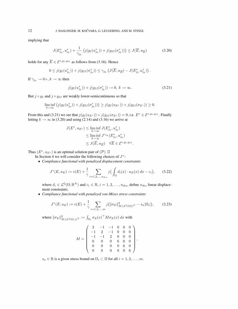
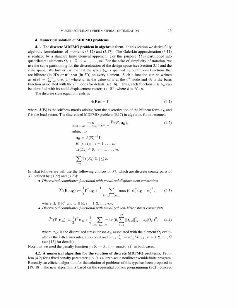
Example 1. We consider a cubic design domain which is loaded in the vertical directionin the center of its top and bottom surfaces and fixed close to the corners of the bottomsurface (see Fig. 4.1). The cube is discretized by 27.000 finite elements. First, we minimizethe compliance of the structure without assuming any additional constraints. Fig. 4.2 shows:

• the optimal material density computed by the trace of the material tensor on everyelement (a);

• the principal material orientation computed via the eigenvector associated with theprincipal eigenvector of the Voigt tensor (b);

• the deformation of the loaded body (c).One can observe that the whole body deforms in the direction of the applied vertical load.

Now we add a number of the displacement constraints by using (4.3), in order to forcethe loaded nodes on the bottom of the structure to deform in the direction opposite to theapplied load. We solve the resulting multidisciplinary problem by Algorithm I. The resultsare depicted in Fig. 4.3. It can be clearly seen that the loaded structure deforms in the desireddirection. Because the applied volume bound is the same in both cases, one can expect that thecompliance of the optimal structure becomes worse after adding the displacement constraints.Precisely that is seen in Fig. 4.3c: the loaded nodes on the top surface are deformed muchmore in the direction of the load compared to the unconstrained case. Statistics for bothnumerical experiments are summarized in Table 4.1.

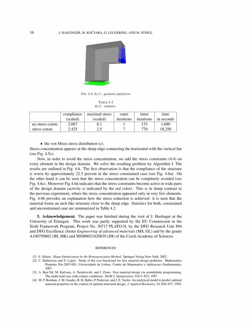
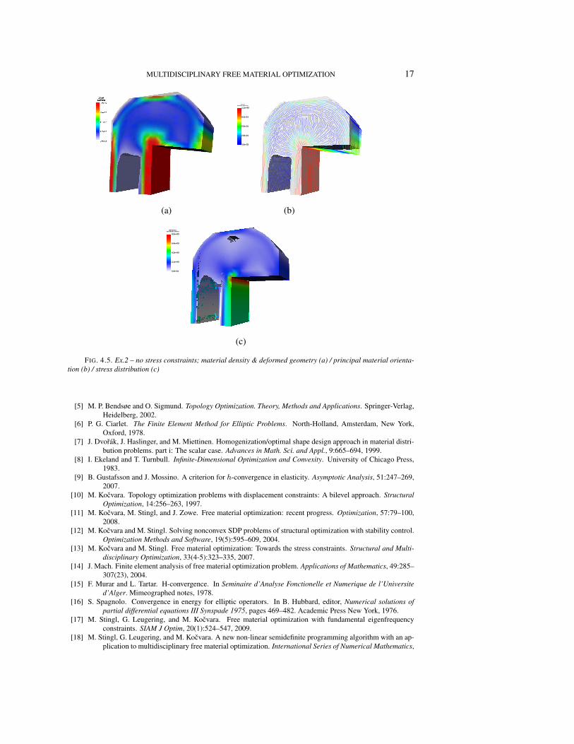
Example 2. In our second example we consider a three-dimensional L-shaped geometry.The design domain clamped at the bottom is loaded by a vertical load on the right hand sideof the structure (see Fig. 4.4). This time the design space is discretized by approximately10.000 finite elements. Again we first minimize the compliance of the structure without anyadditional constraint. Fig. 4.5 shows:

• the optimal material density computed by the trace of the material tensor on everyelement together with the deformation of the body (a);

• the principal material orientation (b);


FIG. 4.1. Ex.1 – geometry and forces

1.1e-021.1e-02

2.5e-012.5e-01

5.0e-015.0e-01

7.4e-017.4e-01

9.8e-019.8e-01

Actor V1:Actor V1:Streamline EigenvalueStreamline Eigenvalue

(a) (b) (c)

FIG. 4.2. Ex.1 – no displacement constraints; material density (a) / principal material orientation (b) / de-formed body (c)


9.8e-039.8e-03

2.5e-012.5e-01

5.0e-015.0e-01

7.4e-017.4e-01

9.8e-019.8e-01

(a) (b) (c)

FIG. 4.3. Ex.1 – with displacement constraints; material density (a) / principal material orientation (b) /deformed body (c)

TABLE 4.1Ex.1 – statistics.

compliance outer inner time(scaled) iterations iterations in seconds

no displ. constr. 0.606 1 250 11,130displ. constr. 8.01 8 776 35,640

outer iterations: number of iterations required by Algorithm Iinner iterations: total number of iterations reported by PENSCP


FIG. 4.4. Ex.2 – geometry and forces

TABLE 4.2Ex.2 – statistics.

compliance maximal stress outer inner time(scaled) (scaled) iterations iterations in seconds

no stress constr. 2.007 8.1 1 133 1,680stress constr. 2.425 2.5 7 770 18,250

• the von Mises stress distribution (c).Stress concentration appears at the sharp edge connecting the horizontal with the vertical bar(see Fig. 4.5c).

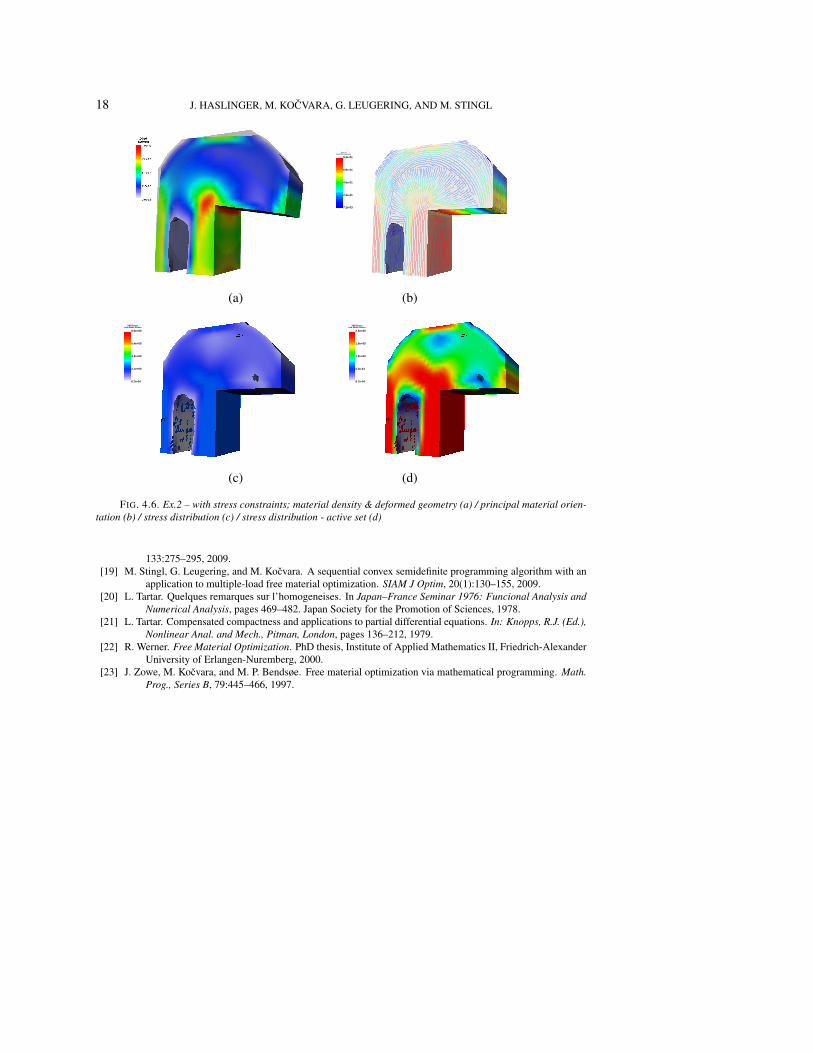
Now, in order to avoid the stress concentration, we add the stress constraints (4.4) onevery element in the design domain. We solve the resulting problem by Algorithm I. Theresults are outlined in Fig. 4.6. The first observation is that the compliance of the structureis worse by approximately 22.5 percent in the stress constrained case (see Fig. 4.6a). Onthe other hand it can be seen that the stress concentration can be completely avoided (seeFig. 4.6c). Moreover Fig.4.6d indicates that the stress constraints become active in wide partsof the design domain (activity is indicated by the red color). This is in sharp contrast tothe previous experiment, where the stress concentration appeared only in very few elements.Fig. 4.6b provides an explanation how the stress reduction is achieved: it is seen that thematerial forms an arch like structure close to the sharp edge. Statistics for both, constrainedand unconstrained case are summarized in Table 4.2.

5. Acknowledgement. The paper was finished during the visit of J. Haslinger at theUniversity of Erlangen. This work was partly supported by the EU Commission in theSixth Framework Program, Project No. 30717 PLATO-N, by the DFG Research Unit 894and DFG Excellence cluster Engineering of advanced materials (MS, GL) and by the grantsA100750802 (JH, MK) and MSM0021620839 (JH) of the Czech Academy of Sciences.

REFERENCES

[1] F. Allaire. Shape Optimization by the Homogenization Method. Springer-Verlag New-York, 2002.[2] C. Barbarosie and S. Lopez. Study of the cost functional for free material design problems. Mathematics

Preprints Pre-2007-003, Universidade de Lisboa, Centro de Matematica e Aplicacoes Fundamentais,2007.

[3] A. Ben-Tal, M. Kocvara, A. Nemirovski, and J. Zowe. Free material design via semidefinite programming.The multi-load case with contact conditions. SIAM J. Optimization, 9:813–832, 1997.

[4] M. P. Bendsøe, J. M. Guades, R. B. Haber, P. Pedersen, and J. E. Taylor. An analytical model to predict optimalmaterial properties in the context of optimal structural design. J. Applied Mechanics, 61:930–937, 1994.



3.6e-033.6e-03

2.8e-012.8e-01

5.5e-015.5e-01

8.2e-018.2e-01

1.1e+001.1e+00

(a) (b)

VM Stress:VM Stress:von Mises Stressvon Mises Stress

5.5e-045.5e-04

2.1e+002.1e+00

4.3e+004.3e+00

6.4e+006.4e+00

8.5e+008.5e+00

(c)

FIG. 4.5. Ex.2 – no stress constraints; material density & deformed geometry (a) / principal material orienta-tion (b) / stress distribution (c)

[5] M. P. Bendsøe and O. Sigmund. Topology Optimization. Theory, Methods and Applications. Springer-Verlag,Heidelberg, 2002.

[6] P. G. Ciarlet. The Finite Element Method for Elliptic Problems. North-Holland, Amsterdam, New York,Oxford, 1978.

[7] J. Dvorak, J. Haslinger, and M. Miettinen. Homogenization/optimal shape design approach in material distri-bution problems. part i: The scalar case. Advances in Math. Sci. and Appl., 9:665–694, 1999.

[8] I. Ekeland and T. Turnbull. Infinite-Dimensional Optimization and Convexity. University of Chicago Press,1983.

[9] B. Gustafsson and J. Mossino. A criterion for h-convergence in elasticity. Asymptotic Analysis, 51:247–269,2007.

[10] M. Kocvara. Topology optimization problems with displacement constraints: A bilevel approach. StructuralOptimization, 14:256–263, 1997.

[11] M. Kocvara, M. Stingl, and J. Zowe. Free material optimization: recent progress. Optimization, 57:79–100,2008.

[12] M. Kocvara and M. Stingl. Solving nonconvex SDP problems of structural optimization with stability control.Optimization Methods and Software, 19(5):595–609, 2004.

[13] M. Kocvara and M. Stingl. Free material optimization: Towards the stress constraints. Structural and Multi-disciplinary Optimization, 33(4-5):323–335, 2007.

[14] J. Mach. Finite element analysis of free material optimization problem. Applications of Mathematics, 49:285–307(23), 2004.

[15] F. Murar and L. Tartar. H-convergence. In Seminaire d’Analyse Fonctionelle et Numerique de l’Universited’Alger. Mimeographed notes, 1978.

[16] S. Spagnolo. Convergence in energy for elliptic operators. In B. Hubbard, editor, Numerical solutions ofpartial differential equations III Synspade 1975, pages 469–482. Academic Press New York, 1976.

[17] M. Stingl, G. Leugering, and M. Kocvara. Free material optimization with fundamental eigenfrequencyconstraints. SIAM J Optim, 20(1):524–547, 2009.

[18] M. Stingl, G. Leugering, and M. Kocvara. A new non-linear semidefinite programming algorithm with an ap-plication to multidisciplinary free material optimization. International Series of Numerical Mathematics,



7.2e-037.2e-03

2.4e-012.4e-01

4.6e-014.6e-01

6.9e-016.9e-01

9.2e-019.2e-01

(a) (b)


8.7e-048.7e-04

2.1e+002.1e+00

4.3e+004.3e+00

6.4e+006.4e+00

8.5e+008.5e+00


8.7e-048.7e-04

6.3e-016.3e-01

1.3e+001.3e+00

1.9e+001.9e+00

2.5e+002.5e+00

(c) (d)

FIG. 4.6. Ex.2 – with stress constraints; material density & deformed geometry (a) / principal material orien-tation (b) / stress distribution (c) / stress distribution - active set (d)

133:275–295, 2009.[19] M. Stingl, G. Leugering, and M. Kocvara. A sequential convex semidefinite programming algorithm with an

application to multiple-load free material optimization. SIAM J Optim, 20(1):130–155, 2009.[20] L. Tartar. Quelques remarques sur l’homogeneises. In Japan–France Seminar 1976: Funcional Analysis and

Numerical Analysis, pages 469–482. Japan Society for the Promotion of Sciences, 1978.[21] L. Tartar. Compensated compactness and applications to partial differential equations. In: Knopps, R.J. (Ed.),

Nonlinear Anal. and Mech., Pitman, London, pages 136–212, 1979.[22] R. Werner. Free Material Optimization. PhD thesis, Institute of Applied Mathematics II, Friedrich-Alexander

University of Erlangen-Nuremberg, 2000.[23] J. Zowe, M. Kocvara, and M. P. Bendsøe. Free material optimization via mathematical programming. Math.

Prog., Series B, 79:445–466, 1997.

Documents

MULTIDISCIPLINARY FREE MATERIAL … FREE MATERIAL OPTIMIZATION J. HASLINGER , M. KOCVARAˇ y, G. LEUGERINGz, AND M. STINGLx Abstract. We present a mathematical framework for the so-called