Embed Size (px)
Citation preview

MULTIDISCIPLINARY DESIGN OPTIMIZATION OF AN
EXTREME ASPECT RATIO HALE UAV
A Thesis
presented to
the Faculty of the California Polytechnic State University,
San Luis Obispo
In Partial Fulfillment
of the Requirements for the Degree
Master of Science in Aerospace Engineering
by
Bryan J. Morrisey
June 2009

ii
© 2009 Bryan J. Morrisey
ALL RIGHTS RESERVED

iii
COMMITTEE MEMBERSHIP
Title: Multidisciplinary Design
Optimization of an Extreme Aspect
Ratio HALE UAV
Author: Bryan J. Morrisey
Date Submitted: June 2009
Committee Chair: Dr. Robert A. McDonald
Committee Member: Dr. David D. Marshall
Committee Member: Dr. Tim Takahashi
Committee Member: Dr. John Dunning

iv
ABSTRACT
Multidisciplinary Design Optimization of an Extreme Aspect Ratio HALE UAV
Bryan J. Morrisey
Development of High Altitude Long Endurance (HALE) aircraft systems is part
of a vision for a low cost communications/surveillance capability. Applications of a multi
payload aircraft operating for extended periods at stratospheric altitudes span military and
civil genres and support battlefield operations, communications, atmospheric or
agricultural monitoring, surveillance, and other disciplines that may currently require
satellite-based infrastructure. Presently, several development efforts are underway in this
field, including a project sponsored by DARPA that aims at producing an aircraft that can
sustain flight for multiple years and act as a pseudo-satellite. Design of this type of air
vehicle represents a substantial challenge because of the vast number of engineering
disciplines required for analysis, and its residence at the frontier of energy technology.
The central goal of this research was the development of a multidisciplinary tool
for analysis, design, and optimization of HALE UAVs, facilitating the study of a novel
configuration concept. Applying design ideas stemming from a unique WWII-era project,
a “pinned wing” HALE aircraft would employ self-supporting wing segments assembled
into one overall flying wing. The research effort began with the creation of a
multidisciplinary analysis environment comprised of analysis modules, each providing
information about a specific discipline. As the modules were created, attempts were made
to validate and calibrate the processes against known data, culminating in a validation

v
study of the fully integrated MDA environment. Using the NASA / AeroVironment
Helios aircraft as a basis for comparison, the included MDA environment sized a vehicle
to within 5% of the actual maximum gross weight for generalized Helios payload and
mission data. When wrapped in an optimization routine, the same integrated design
environment shows potential for a 17.3% reduction in weight when wing thickness to
chord ratio, aspect ratio, wing loading, and power to weight ratio are included as
optimizer-controlled design variables.
Investigation of applying the sustained day/night mission requirement and
improved technology factors to the design shows that there are potential benefits
associated with a segmented or pinned wing. As expected, wing structural weight is
reduced, but benefits diminish as higher numbers of wing segments are considered. For
an aircraft consisting of six wing segments, a maximum of 14.2% reduction in gross
weight over an advanced technology optimal baseline is predicted.

vi
ACKNOWLEDGEMENTS
I am greatly indebted to many of my friends, peers, and mentors for all of their
support through my career at Cal Poly. Their help has allowed me to keep a balanced and
exciting life despite long hours spent at school and in the lab.
I was lucky enough to meet Dr. McDonald early in both his and my time at the
university. His enthusiasm for all things aircraft and seemingly unlimited databases of
aircraft information and stories kept the education fresh and interesting. Over the past
several years I have been employed by the Aerospace Department under both Dr.
McDonald and Dr. Marshall, allowing me to exercise my knowledge while paying my
rent, and I thank you both for that. Dr. Takahashi has provided valuable insight into
several of the methods and processes contained herein, something greatly appreciated
considering the hectic schedules and travel time required. Also I would like to thank Dr.
Dunning for his enthusiasm with this project, as well as the industry connections he
facilitated. Lastly, to all the professors, instructors, and mentors of my past, thank you so
much for all of your hard work. My experience teaching the sophomores here has given
me a new perspective towards the work you do; it is truly a service to the nation.
Now, to all of my friends and roommates over the years, I owe you an enormous
debt of gratitude. To the aero folk, the amount of sleep lost and stress imposed on our
lives would break any lesser student, and I am glad that during the hardest times I always
had a bunch of friends to fall back on, commiserate with, or study with. Doing this alone
would be impossible. For the non aero friends, let’s just say I don’t want to think about
how I’d have turned out if it weren’t for you all. Thanks for being there when I needed a

vii
night off from school, I’m sure I still owe many of you a beer, so don’t be shy about
cashing in. David and Ryan, you guys rock. Putting up with all of my shenanigans must
have been trying at times, not to mention the weeks where we wouldn’t get to hang out
because of school. I hope to see you often in the future, and keep the great times rolling.
Finally, I cannot go without a strong nod to Human League, the men, the myth, the
legend, and my senior design team. You all gave me confidence that among our
engineering brethren, there are others who value having fun as much as doing good work,
and are capable of both.
In addition to my friends and colleagues, I must thank my family for everything
they have sacrificed to see me through to this point. Mom and Dad, what can I say except
that I love you and could not have asked for anything more. I would consider myself
lucky to one day have a family as strong as the one you have built, but I do not doubt that
you have given me the tools to do so. Danielle, it is fun to watch you grow up a couple
years behind me, and I am very excited to see where your life will lead you. You
definitely have great things ahead. To Nonna, Poppop, and all the rest of my family, it is
unfortunate that we are so geographically separated, but it makes me appreciate the times
we are together just that much more. I love you all, and thank you for everything.

viii
TABLE OF CONTENTS
LIST OF TABLES ........................................................................................................... xi
LIST OF FIGURES ....................................................................................................... xiii
NOMENCLATURE ...................................................................................................... xvii
I. INTRODUCTION....................................................................................................... 1
Motivation ..................................................................................................................... 1
Electric Aircraft Background ........................................................................................ 4
History of Electric Propulsion ................................................................................ 4
Aeronautical Solar Technology .............................................................................. 7
Large Solar Aircraft ................................................................................................ 9
Extreme Aspect Ratio Concept .................................................................................... 13
II. PROBLEM STATEMENT ................................................................................ 15
III. METHODOLOGY ............................................................................................. 17
Optimization Architecture ........................................................................................... 17
Design Variables ................................................................................................... 20
Optimizer Constraints ........................................................................................... 22
Multidisciplinary Integration ...................................................................................... 27
Mission Analysis ......................................................................................................... 30
Aerodynamics .............................................................................................................. 34

ix
Induced Drag ......................................................................................................... 34
Parasite Drag ......................................................................................................... 35
Drag Polar Utilization ........................................................................................... 37
Drag Polar Validation ........................................................................................... 43
Electrical Energy Modules ......................................................................................... 46
Solar Energy Generation ....................................................................................... 46
Energy Storage ...................................................................................................... 48
Daily Energy Model .............................................................................................. 50
Propulsion ............................................................................................................. 52
Energy System Weights ........................................................................................ 55
Structures .................................................................................................................... 57
Weights ................................................................................................................. 61
Performance ................................................................................................................ 62
The Integrated Environment ....................................................................................... 66
IV. TOOL VALIDATION ........................................................................................ 67
Maximum Lift Coefficient Response ........................................................................... 71
Propeller Efficiency .................................................................................................... 73
Target Altitude ............................................................................................................ 75
Night Flight and Battery Requirement ........................................................................ 76

x
V. OPTIMIZING BASELINE ARCHITECTURE .............................................. 79
Stage I: Power and Wing Loading as Design Variables ............................................ 81
Stage II: Adding Aspect Ratio as a Design Variable .................................................. 84
Stage III a: Full Optimization of “Daytime Plus” Mission ........................................ 87
Stage III b: Four Variable Optimization of Long Endurance Baseline ...................... 92
Stage IV: Full Optimization of Long Endurance Baseline ......................................... 95
Single Wing Segment Aircraft Baselines................................................................... 101
Different Payloads: Weight and Power Requirement ............................................... 104
VI. SEGMENTED WING OPTIMIZATION ...................................................... 107
Two Segment Wing .................................................................................................... 108
Additional Wing Segments ........................................................................................ 117
CONCLUSION ............................................................................................................. 122
FUTURE WORK .......................................................................................................... 125
REFERENCES .............................................................................................................. 127

xi
LIST OF TABLES
Table 1 - Characteristics of Common Batteries [11] .......................................................... 6
Table 2 – Initial Optimizer Design Variables ................................................................... 20
Table 3 - Additional Design Variables ............................................................................. 21
Table 4 - Discrete Variables ............................................................................................. 22
Table 5 - Fundamental Design Constraints ....................................................................... 25
Table 6 - Mission Analysis I/O ......................................................................................... 33
Table 7 – General Power Train Efficiencies ..................................................................... 53
Table 8 - Specific Power Train Efficiencies [36] ............................................................. 53
Table 9 - Helios Specifications [21] ................................................................................. 68
Table 10 - Configuration Variables for Validation Case .................................................. 68
Table 11 - Baseline Validation Results ............................................................................. 69
Table 12 - Stage I Baseline Optimization Summary ........................................................ 82
Table 13 - Stage II Optimization Summary ...................................................................... 84
Table 14 - Stage III(a) Optimization Summary ................................................................ 88
Table 15 - Optimization Data Summary ........................................................................... 91
Table 16 - Parameters Defining the Long Endurance Baseline ........................................ 93
Table 17 - Stage III(b) Optimization Summary ................................................................ 93
Table 18 - Stage IV Optimization Summary .................................................................... 95
Table 19 - Focused Start Point Optimization Summary ................................................... 98
Table 20 - Baseline Aircraft Summary ........................................................................... 103
Table 21 - Payload Study Optima Comparison .............................................................. 106

xii
Table 22 – Two Segment Wing Optimization Summary ................................................ 108
Table 23 - Average Values for Solution Clusters ........................................................... 115

xiii
LIST OF FIGURES
Figure 1 - Fred Militky's Silentius (left) and Hi-Fly (right) [10] ........................................ 4
Figure 2 - Mattel SuperStar [10] ......................................................................................... 5
Figure 3 - Sunrise II Flight Preparation [9] ........................................................................ 7
Figure 4 - Solong Multi Day Solar Aircraft (http://machinedesign.com) ........................... 8
Figure 5 - The Gossamer Penguin in Flight [9] .................................................................. 9
Figure 6 - Solar Challenger Flying Over the English Channel ........................................ 10
Figure 7 - Solar Aircraft in the ERAST Program [20] ...................................................... 11
Figure 8 - Helios High Altitude Configuration [20] ......................................................... 12
Figure 9 - Early Air Force Wingtip Coupled Flight [24] .................................................. 13
Figure 10 - Extreme Aspect Ratio Concept ...................................................................... 14
Figure 11 - HALE UAV Mission Profile .......................................................................... 15
Figure 12 - Theoretical Aircraft Design Structure Matrix ................................................ 19
Figure 13 - Classical Aircraft Sizing Process ................................................................... 27
Figure 14 - Multidisciplinary Design Analysis and Optimization Architecture ............... 30
Figure 15 - Approximation of Climb ................................................................................ 32
Figure 16 - Comparison of Mission Analysis Methods .................................................... 33
Figure 17 - General Wing Modeled in AVL With Loading Distribution ......................... 34
Figure 18 - General Baseline Geometry ........................................................................... 38
Figure 19 - Drag Polars During the Helios Baseline Analysis ......................................... 39
Figure 20 - Reynolds' Number Based on Chord ............................................................... 40
Figure 21 - Parasite Drag Breakdown, Component Drag Counts ..................................... 40

xiv
Figure 22 - Effect of Aspect Ratio on Drag ...................................................................... 41
Figure 23 - Lift to Drag Ratio ........................................................................................... 42
Figure 24 - GlobalFlyer Modeled in VSP for Drag Validation ........................................ 43
Figure 25 - Cruise Drag Polar for GlobalFlyer ................................................................ 44
Figure 26 - Parasite Drag Buildup for GlobalFlyer, Component Drag Counts ................ 44
Figure 27 - Effect of Wing Thickness on Drag ................................................................. 45
Figure 28 - Basis for Available Solar Energy Models [14], [36], [37] ............................. 48
Figure 29 - Model for Available and Required Power (above) and Resulting Extra Power
(below) .............................................................................................................................. 50
Figure 30 - Energy Storage Charge Profile ....................................................................... 51
Figure 31 - HALE UAV Power Systems .......................................................................... 52
Figure 32 - Helios Wing Structural Arrangement [50] ..................................................... 58
Figure 33 - Structural Analysis Process ............................................................................ 58
Figure 34 - General Spanwise Loading Distribution ........................................................ 59
Figure 35 - General Spanwise Shear and Moment Diagrams ........................................... 59
Figure 36 - Spar Wall Thickness Profile ........................................................................... 60
Figure 37 - Performance Analysis Process ....................................................................... 64
Figure 38 - Absolute Ceiling (kft) .................................................................................... 64
Figure 39 - Max Rate of Climb (ft/min) ........................................................................... 65
Figure 40 – Final MDO Tool Schematic .......................................................................... 66
Figure 41 - Baseline Weight Breakdown .......................................................................... 70
Figure 42 - CL for Minimum Power .................................................................................. 71
Figure 43 - Response to CLmax Perturbation ...................................................................... 72

xv
Figure 44 - Response to ηP Perturbation ........................................................................... 74
Figure 45 - Response to Target Altitude Perturbation ...................................................... 76
Figure 46 - Response to Night Flight Requirement .......................................................... 78
Figure 47 - Response to Improved Battery Technology ................................................... 78
Figure 48 - Optimal Baseline Development Procedure .................................................... 80
Figure 49 - Scaled Design Variable History ..................................................................... 82
Figure 50 - Stage I Objective Function History ................................................................ 83
Figure 51 - Stage I Optimization Component Weights .................................................... 84
Figure 52 - Stage II Scaled Design Variable History ....................................................... 85
Figure 53 - Stage II Objective Function History .............................................................. 86
Figure 54 - Comparison of Optimal Weight Breakdowns ................................................ 86
Figure 55 - Maximum Constraint Violation History ........................................................ 87
Figure 56 - Stage III(a) Design Variable History ............................................................. 88
Figure 57 - Stage III(a) Objective Value History ............................................................. 89
Figure 58 - Progression of Optimal Weight Breakdowns ................................................. 89
Figure 59 - Spar Design for Two Configurations ............................................................. 90
Figure 60 - Weight Breakdown for the ATLEB Compared to Earlier Results ................. 94
Figure 61 - Stage IV Design Variable History.................................................................. 96
Figure 62 - Comparison of Stage IV Weight to Previous Optima .................................... 97
Figure 63 - Weight Breakdown for Revised Stage IV Optimization ................................ 98
Figure 64 - Weight Comparison for Progressive Baseline Optimal Configurations ........ 99
Figure 65 - Desired Battery Charge Profile .................................................................... 100
Figure 66 - Helios Proxy Alongside Two Optimal Baselines ......................................... 101

xvi
Figure 67 - Comparison of Optimized Baseline Aircraft to NASA ERAST Family ...... 102
Figure 68 - Weight Breakdown for Different Payload Weights ..................................... 104
Figure 69 - Battery, Solar, and Wing Weight Sensitivity to Payload ............................. 105
Figure 70 - Weight Breakdown for Different Payload Power ........................................ 105
Figure 71 – Two Segment Objective Function History .................................................. 109
Figure 72 - Weight Comparison for Two Segment Aircraft ........................................... 110
Figure 73 - Plot Matrix of All Optimization Cases for a Two Segment Platform .......... 111
Figure 74 – Two Segment MDO Solution Space ........................................................... 112
Figure 75 – Two Segment Solutions Sorted by Gross Weight ....................................... 113
Figure 76 - Design Variable History for Anomalous Solutions ..................................... 114
Figure 77 - Design Variable History for Attractive Solutions ........................................ 115
Figure 78 - Two Segment Solutions: Reynolds' Number ............................................... 116
Figure 79 - Weight Breakdown Comparison of Multiple Wing Segment Configs ........ 117
Figure 80 - Optimal Wing Thickness for Multiple Wing Segments ............................... 118
Figure 81 - Optimal Wing Chord for Multiple Wing Segments ..................................... 119
Figure 82 - Optimal Sref for Multiple Wing Segments .................................................... 119
Figure 83 - Optimal Solar Coverage (Percent) ............................................................... 120
Figure 84 - Optimal Gross Weight for Multiple Wing Segments ................................... 120
Figure 85 - Optimal Wing Loading for Multiple Wing Segments .................................. 121
Figure 86 - Optimal Aspect Ratio for Multiple Wing Segments .................................... 121

xvii
NOMENCLATURE
A = area
AR = aspect ratio
ATLEB = Advanced Technology Long
Endurance Baseline
b = wing span
BFGS = Broyden-Fletcher-Goldfarb-Shanno
c = optimizer inequality constraints
cc = cubic centimeter
CD = drag coefficient
ceq = optimizer equality constraints
CL = finite wing lift coefficient
DSM = Design Structure Matrix
E = energy
e = span efficiency factor, Oswald’s
efficiency
EDET = Empirical Drag Estimation
Technique
f = optimizer objective function
F.F. = form factor
fc = fuel cell
ft = foot

xviii
h = altitude
HALE = High Altitude Long Endurance
hr = hour
I = solar irradiance, current
I/O = input-output
in = inch
kg = kilogram
KT = Kuhn-Tucker
L = liter
L/D = lift to drag ratio
lb = lower bound, pound force
Li-Ion = Lithium Ion
Li-Po = Lithium Polymer
Li-S = Lithium-Sulfur
MDA = Multidisciplinary Analysis
MDAO = Multidisciplinary Analysis and
Optimization
MDO = Multidisciplinary Design
Optimization
mo = months
N = number of components
n = rotational speed, component index
NiCd = Nickel-Cadmium

xix
Ni-MH = Nickel metal-hydride
OBD = Optimizer Based Decomposition
P = power
PEM = Proton Exchange Membrane fuel cell
POBD = Partial Optimizer Based
Decomposition
PoW = power to weight ratio
PTMEB = Proven Technology Medium
Endurance Baseline
Q = torque
Re = Reynolds’ number
S = area
SQP = Sequential Quadratic Programming
SREF, Sref = wing reference area
SWET, Swet = wetted area
T = thrust
t = time
t/c = wing thickness to chord ratio
UAV = Unmanned Aerial Vehicle
ub = upper bound
V = Volt, Velocity
W = Watt, Weight (lbs)
WoS = wing loading

xx
x = design variable
XAR = eXtreme Aspect Ratio
Δ = change, delta
ρ = density
η = efficiency
κsol_coverage = percent of the wing covered with
solar cells
κwatt = power conversion factor
Subscripts
Asol = area density of solar system
BATT = battery
batt_req = required to be stored in the battery
F = flat plate friction drag
FC, fc = fuel cell
G = gearbox
i = induced drag contribution
INC = incompressible
M = motor
o = parasite drag contribution
P = propeller
PMD = power management and distribution

xxi
R = required energy at propeller
ref = reference
s = shaft torque, stored energy, specific
excess power
SC = speed controller
sls = sea level static
sol = solar
SRC = source (batteries, fuel cell, etc.)
TO, to = takeoff
tot = total

1
I. INTRODUCTION
Motivation
Development of High Altitude Long Endurance (HALE) aircraft systems has long
been part of a vision for a low cost communications/surveillance capability [1], [2], [3].
Applications of a multi payload aircraft operating for extended periods at stratospheric
altitudes span military and civil genres and support tactical battlefield operations,
communications, atmospheric monitoring, precise agricultural and wildfire monitoring,
surveillance, and other disciplines requiring satellite-based infrastructure or high
resolution imagery [4]. Currently, the Defense Advanced Research Projects Agency
(DARPA) is requesting proposals for an aircraft that can sustain flight for multiple years
and act as a pseudo-satellite for intelligence, surveillance, and reconnaissance missions
[5]. Design of this and any type of air vehicle represents a substantial challenge because
of the vast number of engineering disciplines required for analysis. In addition, some
tools and analysis methods used in the design of aircraft with more conventional missions
may not be applicable to certain types of HALE vehicles. In the modern competitive
environment surrounding the manufacture of aircraft systems, oftentimes simply meeting
the customer’s requirements may not win a contract. Instead, the proposed system must
also represent the optimum vehicle for the customer needs [6]. This focus on finding an
optimal solution places some additional requirements on the design process itself.
Searching for an overall optimal solution involves broadening the trade space
and allowing a large number of variables. These high degree of freedom environments
are not handled well by a sequential design process [7]. Also, with highly multivariate

2
design spaces, analyzing the sensitivities to each variable individually and relating this
information to a whole system sensitivity is a daunting task. One method for mitigating
many of the challenges associated with designing complex aeronautical systems is to
compile the individual disciplines and analysis methods into one environment, allowing
for better organization of data flow, and more efficient communication. This may be
accomplished on a small scale by simply bringing codes together on one machine, or in a
larger sense by allowing physically separated flight science groups to wrap their analyses
for remote use. Once assembled, multidisciplinary analysis, design, and optimization
techniques can be applied in the hopes of allowing more broad design spaces and
providing a clearer view of system drivers and sensitivities.
With an integrated HALE design environment in place, it is possible to perform
parametric studies to investigate areas of potential improvement over current concepts. In
essence, we are looking for the active constraints on the design, or the design drivers.
Wing design and propulsion systems are the two main aspects of HALE vehicles that are
driven by mission requirements, and consequently present the greatest opportunity for
system improvements. Accordingly, when considering new or revolutionary design
concepts, these two areas should be of primary focus. Generally, HALE aircraft of the
past and present, like the U2, Helios, or Global Hawk exhibit high aspect ratio wings that
allow the aircraft to achieve the altitudes of interest. Sacrifices are made, however,
because with a high aspect ratio planform comes high wing bending moments,
unfavorable dynamic structural responses, and large deflections. In the propulsion arena,
many current designs feature distributed propulsion, advanced propeller design, and a
strong coupling between propulsion and flight controls. Closely related to propulsion is

3
the energy source for the aircraft. Most modern internal combustion architectures cannot
satisfy the persistent operation requirements of current HALE missions like Vulture or
the Communications Relay posed by the AIAA in 2007 that stipulate months to years of
continuous flight [8]. As a result, much effort has been devoted to development of
environmental energy collection, high energy density storage devices, and other
alternative energy concepts [5].
The intent of this research is to evaluate revolutionary changes to HALE aircraft
architecture, using state of the art propulsion and energy concepts while breaking new
ground for wing design. Wing aspect ratio is the primary characteristic of wing design for
the purposes of this study, and the NASA / AeroVironment Helios aircraft set the current
threshold for demonstrated all-electric flight with an aspect ratio of 31. With a new wing
concept, it may be possible to push this envelope of high aspect ratio platforms, while
simultaneously mitigating problems associated with highly flexible aircraft structures. An
integration of architecture-independent design codes into an optimization environment
enables identification of constraints that emerge when exploring extreme-aspect-ratio
concepts. These constraints take the form of structural and energy requirements such as
max stress or minimum specific energy storage density, as well as mission operation
requirements that take into account things like available runways and hangers for aircraft
with extremely long wingspan. One goal of this paper is to find the area of diminishing
returns for wing aspect ratio is such behavior exists, and discuss why and how certain
constraints become active. In addition, the work diverges from combustion-based sizing
methods and focuses on generalizing the design process for energy-optimized systems
and all-electric aircraft.

4
Electric Aircraft Background
History of Electric Propulsion
Electric propulsion systems in aircraft date back to the 1950’s when model
aircraft enthusiasts and hobbyists first became successful in the field. The first officially
recorded electrically powered flight occurred in June of 1957 with Colonel H.J. Taplin’s
retro-fitted Radio Queen. Weighing in at 8 lbs, the radio controlled model utilized
silver/zinc battery cells and a government surplus electric motor in lieu of the stock 3.5 cc
diesel engine [9]. Several years later, a coreless motor with an integrated gearbox initially
developed for remote control cameras would be adapted to model aircraft. Called the
Micromax, this motor was at the heart of the first model developed by Fred Militky for
the public, the Silentius [10]. Militky continued development of electric aircraft with the
Hi-Fly, working towards the goal of manned electric flight. Figure 1 shows both aircraft.
Figure 1 - Fred Militky's Silentius (left) and Hi-Fly (right) [10]

5
Later, in the early 1970’s, the first widely commercially available electric model was
introduced. Dubbed the Super Star, this aircraft was rechargeable and included a rudder
as its only flight control [10].
Figure 2 - Mattel SuperStar [10]
Advances in energy storage devices over the last 50 years have drastically
affected our ability to apply electric propulsion to air vehicles. The main difficulty in
flying an aircraft electrically is that the power sources have very low energy densities.
Through the early 1990’s, the best batteries available were nickel-cadmium or nickel
metal-hydride. It wasn’t until 1991 when lithium-ion batteries were released that the
technology really saw a drastic increase in performance. Lithium-ion batteries were then
modified to use a composite solid electrolyte. The resulting lithium-polymer batteries
were introduced in 1996. Several characteristics of these batteries are included in Table 1.
Of particular interest to aircraft applications is the energy density of the battery.
Compared to the early nickel-cadmium based cells’ 30-80 W-hr/kg, the lithium
technologies offers drastic increases, potentially as high as 200 W-hr/kg [11].

6
Table 1 - Characteristics of Common Batteries [11]
Characteristic NiCd NiMH Li-Ion Li-Po
Energy Density 40-60 W-hr/kg 30-80 W-hr/kg 160 W-hr/kg 130-200 W-hr/kg
Energy / Vol. 50-150 W-hr/L 140-300 W-hr/L 270 W-hr/L 300 W-hr/L
Power Density 150 W/kg 250-1000 W/kg 1800 W/kg 2800 W/kg
Cycle Eff. 70%-90% 66% 99.90% 99.80%
Lifetime - - 24-36 mo. 24-36 mo.
Life Cycles 2000 cycles 500-1000 cycles 1200 cycles >1000 cycles
Nominal Voltage 1.2 V 1.2 V 3.6 V 3.7 V
More recently, the advent of lithium-sulfur rechargeable batteries has pushed the
envelope of energy density out to 350+ W-hr/kg [12], some sources citing as high as 400.
Unfortunately, the lithium-sulfur batteries currently exhibit a cycle life of around 100
cycles. For HALE UAV applications with mission goals in the vicinity of days to months
of persistent flight, these batteries are promising. If, however, desired endurance is on the
scale of years, as with the DARPA Vulture program, lithium-sulfur batteries are not quite
so attractive. On the positive side, advances in energy density are historically
accompanied by a decrease in cycle life initially, until design refinement brings it back to
acceptable levels [13] so we may expect improvements in the coming years.
When implemented into an aircraft design environment, the energy density of the
batteries, or other energy storage systems, becomes one of the primary indicators of
technology level, and represents a major determinant of aircraft weight. Another method
of energy storage applicable to electric aircraft is the use of fuel cells. In October 2007,

7
NASA presented a feasibility study focused on “Solar Airplanes and Regenerative Fuel
Cells” in which they evaluate the energy storage requirements for year-long continuous
flight. Of course, latitude has an effect on available solar energy, and the required energy
density ranged from 250 W-hr/kg at the equator to 500 W-hr/kg at 45 deg. North [14].
Aeronautical Solar Technology
Supplying energy to onboard storage systems in all electric HALE aircraft must
be performed by some type of environmental energy collection system. Many, if not all
current HALE concepts employ solar power, and its use dates back to1974 when Sunrise
I, lifted off of a dry lake bed in California for a 20 minute solar powered flight. This 27 lb
photovoltaic aircraft flew to 328 ft above ground with 450 watts of supplied solar power.
After sustaining damage during flight, an improved Sunrise II was constructed using
higher efficiency solar cells and lighter structure, increasing the power to weight ratio
from 16.6 W/lb to 26.6 W/lb [9]. Figure 3 shows Sunrise II on the lakebed.
Figure 3 - Sunrise II Flight Preparation [9]
Photovoltaic technology as we know it today appeared first in 1954 with the
development of the silicon photovoltaic cell at Bell Telephone Labs [15]. The first to be
able to convert enough energy from the sun to run conventional electronics, this cell

8
initially exhibited a 4% efficiency. Another major contributor to photovoltaic technology
development was Hoffman Electronics, rolling out a 9% efficient cell in 1958, followed
by 10% in 1959 and 14% in 1960. Development continued as more industries realized the
potential of solar energy, and in 1964 NASA launched the Nimbus satellite powered by a
470 watt solar array [15]. As stated previously, the first application of photovoltaic
technology to aircraft resulted in the successful flights of Sunrise I and II, shortly
followed in Europe by Fred Militky and Solaris. Development of small to medium scale
solar UAVs continues to the present, and in 2005, Alan Cocconi flew Solong, a 23 lb
solar regenerative power UAV that demonstrated 48 hour continuous flight [16]. Figure 4
shows Solong’s 15.6 ft wingspan aircraft as it would land, with the propeller blades
folded aft.
Figure 4 - Solong Multi Day Solar Aircraft (http://machinedesign.com)

9
Large Solar Aircraft
Up to this point, most electric aircraft discussed have been small UAVs, with
payloads ranging from zero to a couple pounds. The question remains, is this a promising
area to explore larger payloads and aircraft? DARPA has expressed the desire for a long
endurance aircraft that can support a payload of 1000 lb and 5 kW [5]. Also, manned
solar flight represents an environmentally friendly option for travel and recreation.
Exploration into larger solar aircraft platforms began with Dr. Paul MacCready and
AeroVironment Inc. Initially, Dr. MacCready explored man-powered flight with the
Gossamer Condor and Gossamer Albatross [17]. These aircraft relied on advanced
lightweight structures and an extremely low wing loading to achieve flight given low
power available from the power plant (pilot). Expanding the aircraft design and
construction techniques to the solar arena, MacCready developed the Gossamer Penguin
(Figure 5), a smaller version of the Albatross with added solar panels.
Figure 5 - The Gossamer Penguin in Flight [9]
R.J. Boucher, designer of the Sunrise UAVs worked with MacCready, supplying parts
from the nonoperational Sunrise aircraft [9]. On May 18, 1980 the Gossamer Penguin

10
became the first manned solar aircraft to demonstrate flight. DuPont, the sponsor for the
Penguin, continued to support this concept by funding Solar Challenger, an aircraft
designed by MacCready to cross the English Channel. On July 7, 1981, Solar Challenger
completed the mission, flying for over 5 hours with no energy storage devices [9].
Figure 6 - Solar Challenger Flying Over the English Channel
Investigation into solar HALE aircraft as platforms for surveillance,
communications, or other related missions began after Solar Challenger demonstrated the
feasibility of solar power for aircraft. This along with the potential for relocatable and
maintainable pseudo-satellites in the atmosphere spurred the development of HALSOL
(High ALititude SOLar vehicle). The goals for the program were to fly above 65,000 ft
during day/night operations. The 440 lb aircraft completed several validation flights
under battery power but was unable to close the loop for solar regenerative energy and
day/night operation and the program ended in 1983 [18].

11
Lessons learned from HALSOL were compiled and in the early 1990’s, the
Ballistic Missile Defense Organization funded an effort to update the airframe with
modern technologies. Wing structures were modified and new solar cells, motors and
propellers were added. The revamped airframe weighed in at 560 lbs and was dubbed
Pathfinder. In 1995 it set an altitude record for solar-powered aircraft at 50,500 ft. and
two years later, the aircraft set a world altitude record for propeller driven aircraft at
71,530 ft [18], [19].
Pathfinder was the first aircraft being evaluated under NASA’s Environmental
Research Aircraft and Sensor Technology (ERAST) program. ERAST was designed to
develop and evaluate new technologies in sensors, light structures, aerodynamics, and
propulsion to support extreme altitude and extreme endurance aircraft configurations
[20]. With the success of Pathfinder, NASA and AeroVironment built a family of aircraft
over the subsequent decade (Figure 7). Each new aircraft exhibited increased wing aspect
ratio and more advanced power and propulsion technologies.
Figure 7 - Solar Aircraft in the ERAST Program [20]
12
Culminating the ERAST program was Helios, the fourth and fifth generations of ERAST
aircraft. Two aircraft were constructed; the first was optimized for high altitude (Figure
8) and the second for long endurance. NASA’s goals for Helios were twofold. First, the
aircraft was to demonstrate sustained flight above 100,000 ft, and second, it was to
sustain flight for 24 hours with at least 14 of those above 50,000 ft altitude. In 2001, the
high altitude configuration of Helios reached a world record altitude of 96,863 ft. and
flew for 40 minutes above 96,000 ft [21]. Unfortunately, the redistribution of weight for
the long endurance configuration included a large point mass at the midpoint of the wing
to house fuel cell equipment. What resulted was an aircraft that didn’t exhibit the same
qualities of a span loaded aircraft as its predecessors, and several control algorithms
encountered errors during a persistent high wing dihedral. The aircraft became unstable
in pitch and was destroyed in flight over the ocean [20].
Figure 8 - Helios High Altitude Configuration [20]

13
Extreme Aspect Ratio Concept
Developing a revolutionary concept for increasing aspect ratio without paying the
penalties commonly associated with doing so is primarily inspired by a somewhat
obscure Air Force research effort in the early 1950s that was itself inspired by German
scientist Dr. Richard Vogt who emigrated to the U.S. after WWII. The initial concept was
that the range of a bomber may be increased by adding “free-floating” wing segments
that are pinned to the bomber wingtips [22]. Also, the U.S. military wanted to examine
the feasibility of utilizing the long range capabilities of bombers like the B-36
Peacemaker or the B-29 Superfortress to tow, carry, or otherwise transport smaller and
more maneuverable fighter aircraft like the F-84 to foreign combat zones. The first
concepts involved the smaller aircraft docking in the bomb bay of the bomber for
parasitic flight to and from the target. In this scenario, the extra aircraft adds parasitic
drag to the bomber, and takes up bomb bay space, while not contributing anything
aerodynamically positive in return [23]. A follow-on effort designated MX-1016 “Tip
Tow” moved the parasite fighter from under the host aircraft to the wingtip [22]. Figure 9
shows a Boeing B-29 in flight with two EF-84 aircraft coupled at the wingtips [24].
Figure 9 - Early Air Force Wingtip Coupled Flight [24]

14
With the new configuration, the parasitic aircraft now contribute additional wingspan to
the bomber, reducing the induced drag [25]. The wingtip coupling mechanisms
underwent some revision under a new project called “Tom-Tom” involving clamps or
jaws on the wingtips of a B-36 [24].
Applying the idea of wingtip coupling to a flying wing HALE aircraft represents a
revolutionary step in the field. Conceptually, each segment of the flying wing would lift
its own weight and comprise a generally self-sufficient aircraft system. Stringing some
number of individually moderate aspect ratio wing segments together to form an extreme
aspect ratio platform allows each segment to benefit from lower structural loads while
simultaneously reaping benefits of an extremely high aspect ratio planform. Figure 10
shows what one such vehicle might look like.
Figure 10 - Extreme Aspect Ratio Concept
In addition to lowering the structural weight fraction of the aircraft, a “pinned
wing” concept may offer the ability to orient solar cells favorably towards the sun. Also,
with a conventional high aspect ratio flying wing configuration, natural frequencies of the
structure can be so low that they approach control response frequencies. If these come too
close together, an aileron deflection, or step input may induce structural resonance rather
than the desired change in flight condition. Considering that the individual wing
segments of the extreme aspect ratio concept have low-to-moderate aspect ratios, they
will be more rigid and exhibit higher natural bending mode frequencies.

15
II. PROBLEM STATEMENT
The central goal of this research is the development of a multidisciplinary tool for
analysis, design, and optimization of High Altitude Long Endurance (HALE) UAVs.
Current and projected future missions for this type of aircraft platform focus on its ability
to provide sustained support for surveillance, communications, or other science missions,
and act as an “atmospheric satellite”. Accordingly, the baseline mission profile consists
of a climb to some stratospheric cruise/loiter altitude, where the aircraft begins mission
operations and enters an extended cruise or loiter flight mode, shown in Figure 11.
Figure 11 - HALE UAV Mission Profile
With an integrated design and analysis environment in place, certain parameters
may be adjusted to approximate current or past proven aircraft configurations in an effort
to calibrate the tool. Next, optimization techniques are applied to a baseline platform,
here represented by flying wing aircraft similar to Helios or the Vulture concept.
Investigation of performance trends and the effect of new technologies, as well as system
sensitivities from parametric studies may be performed at this stage. Considerations are
made throughout the development of the tool to allow a wide range of missions, payload
systems, and potential solutions.
Long Endurance Loiter
Landing Takeoff
Climb Low Power or Gliding Descent
Cruise Cruise
Mission Operations

16
Following the analysis and optimization of a proven platform aircraft, the design
tool is adjusted to study the effect of implementing a segmented wing concept. Again, the
individual flight science modules, or discipline analysis codes are developed to be
flexible and applicable to both single and multiple segment wings. As before, parametric
studies and optimization of the segmented platform reveal design drivers and best
configurations, which may be compared with the results from the proven aircraft study,
as well as actual flown aircraft results.
One of the attractive aspects of a segmented wing platform is the ability to build it
up from identical and self sufficient segments, allowing more flexibility for payloads and
missions. As such, the optimization objective is to develop a platform of identical
segments that minimizes aircraft weight while meeting mission, performance, and
technology constraints. In reality, the goal is minimization of total cost, which may be
composed of both acquisition and operating cost. For the included studies, aircraft cost is
assumed to be well represented by aircraft weight, as suggested in [26]. Also, in a report
prepared for the Suborbital Science Office Earth Science Enterprise of NASA, it is
proposed that a breakthrough in reducing acquisition cost of UAV science missions may
be possible with a new generation of small HALE aircraft with simplified operational
requirements [27]. It is important, however, to consider that all-electric HALE platforms
are pushing the frontier of energy technology, and parameters like the specific energy
density of batteries, or efficiencies of power system components like solar cells, power
conditioning units, speed controllers and motors may greatly affect costs. It is possible to
consider alternative objectives for the optimization that may account for the cost
dependence on technology, such as minimizing required solar efficiency for a mission.

17
III. METHODOLOGY
Development of the multidisciplinary analysis, design, and ultimately
optimization tool begins with a buildup of individual disciplines, each capable of
analyzing both a baseline flying wing/cantilever configuration and a segmented wing
platform. What follows is a description of the approach to optimization, a look into the
integrated multidisciplinary environment, and specifics about the individual disciplinary
analysis methods.
Optimization Architecture
With aircraft weight as the central objective for minimization, parameters
describing the aerodynamic, structural, propulsive, and energetic qualities of the aircraft
are varied to determine preferred configurations that meet applicable constraints. As the
main body of code was developed in MATLAB, the built-in optimizer “fmincon” is used
to minimize a constrained multivariate function. The general form of the optimization
problem is given in (1).
0
0 (1)
Where c represents a set of inequality constraints, ceq represents the equality constraints,
supplemented by lb and ub, the lower and upper bounds enforced on the set of design
variables .
When performing an optimization, fmincon defaults to attempt to use a trust-
region-reflective algorithm, which requires a user supplied gradient for the objective
18
function. Developing an analytical gradient for the entire design process for an aircraft
from conceptual design through mission analysis and preliminary sizing is both difficult
and beyond the scope of the work herein. In addition, several of the analysis modules
utilize pre-compiled binaries or executables, further discouraging any attempt to find the
gradient. Instead, an optimization algorithm must be used that numerically estimates
gradient and Hessian functions. The Optimization Toolbox in MATLAB offers Active-
Set optimization for problems such as this. For Active-Set optimizations, MATLAB
implements sequential quadratic programming (SQP) to choose search directions by
mimicking Newton’s method [28]. Sequential Quadratic Programming approximates the
objective function, generally Wtot( ), as a quadratic function. The method then linearizes
constraints locally and applies Quadratic Programming to approximate the solution. SQP
looks to the Broyden-Fletcher-Goldfarb-Shanno (BFGS) method for updating the Hessian
[29].
Fundamentally, the process employed for designing the UAV is an iterative
process, meaning that from a systems perspective, there is feedback inherent in the data
flow structure. Specifics about the feedback quantities are discussed in the next section,
but how they are handled effects the optimization environment. Two methods were
considered and tested for solving the resulting system of nonlinear equations. The first is
a simple iterative scheme that converges all of the system feedback given initial guesses
for each feedback quantity. Generally referred to as Fixed Point Iteration (FPI), this
scheme provides an intuitive method for solving a system, but no guarantee that a
solution exists. An attempt was made at developing a convergence criteria using
Newton’s Method, but an analytical representation of the whole system is not feasible.

19
The alternative to FPI is a process called Optimizer Based Decomposition (OBD)
where data links in the system of equations are broken and replaced by new design
variables and constraints [30], [31]. Specifically, for the problem of interest here, only the
feedback data links are decomposed, and we designate the process Partial OBD (POBD).
Allowing the optimizer to simultaneously handle the regular design variables and the
requirement for a converged system decreases the run time per iteration and increases the
probability of closing the design, or achieving convergence. In addition, the constraints
on convergence may be held strict or loosened depending on the desired fidelity of the
solution. A simplified and purely theoretical system is presented in Figure 12 to illustrate
the interaction between disciplines. In this system representation, active column elements
are inputs to a module and rows are outputs. Reference [32] gives a thorough description
of the processes for using a diagram like this, but completing a quick system trace reveals
that active cells in the lower triangle represent feedback data paths. A POBD process
operates on these cells to eliminate the need for iterative solving.
Figure 12 - Theoretical Aircraft Design Structure Matrix
A more detailed Design Structure Matrix (DSM) is presented in the next section,
and represents the actual multidisciplinary system implemented for this study.
Geom. X
Aero X X
X Mission Analysis X X
X X X Weights X X
Cost
Perf.
X
X

20
Design Variables
Parameters selected as design variables for this optimization are products of the
approach to conceptual design, mission analysis, and preliminary aircraft design methods
discussed in the next section. As a quick preview, several key characteristics of the
aircraft are specified up front, and an iterative design process (hopefully) converges to a
final configuration. A complete list of inputs to the design environment comprises the set
of all potential design variables, only some of which are actually selected as design
variables for the optimizer, while others represent technology factors, mission
characteristics, or configuration identifiers. The design of experiments for a complex
multivariate optimization problem such as this begins with selecting a basic set of design
variables, leaving the rest as constants that define aspects of the configuration. Table 2
shows the basic set of design variables used.
Table 2 – Initial Optimizer Design Variables
Design Variable
1 Total aspect ratio
2 Wing loading (lb/ft2)
3 Power to weight (W/lb)
4 Wing thickness-to-chord ratio
5 Percent of Sref covered by solar panels
Along with the fundamental design variables of Table 2, there are several other
parameters of the design which may be more effective as optimizer-controlled design

21
variables than predetermined quantities. Table 3 shows these parameters, including the
variables necessary for implementing POBD. The ‘+’ symbol indicates that there are
more than one actual variables associated with the characteristic, that variable can be
thought of as a vector quantity. For example, the battery-pod spanwise locations may be
left to be determined by the optimizer, but there may be 10 pods holding batteries or
payload so that the actual design variable may have dimension [1x5] depending on
symmetry assumptions.
Table 3 - Additional Design Variables
Design Variable
6* Total weight (lb)
7* Wing weight (lb)
8 Cruise Altitude (ft)
8 Payload weight (lb)
9 Payload power requirement (W)
10 + Spar factor of safety, material properties
11 + Spar cross section locations (% span)
12 + Battery or payload pod locations (% spar)
13 + Technology factors
* optimizer-based decomposition variable
Lastly, there are several characteristics of the aircraft that are discrete numbers.
The optimization methods employed do not handle such data types, so when designing
the experiments, each of the variables in Table 4 must be specified for a set of parametric

22
studies or optimization runs. Results may then be compared between the discrete values
to assess potential benefits against additional complexity.
Table 4 - Discrete Variables
Number of wing segments
Number of battery/payload pods
Number of spar cross sections
Optimizer Constraints
Equation (1) states that our system may be subject to either inequality or equality
constraints which may act on the design variables themselves or certain determined
quantities within the system. Decisions about which metrics to use as constraints are a bit
more vague with a HALE UAV platform than with aircraft designed for more
conventional missions. Take, for example, the recent Broad Agency Announcement
delivered by DARPA requesting proposals for a HALE UAV. The requirements supplied
by DARPA are simple and few [5]:
• 5 years uninterrupted operation
• 1000 lb, 5 kW payload
• 99% probability of station-keeping
• High probability of mission success
From a preliminary design point of view, the first two bullets are the only requirements.
Where other categories of aircraft may have a set of point performance requirements

23
explicitly laid out for them, in our case the designer must work diligently to flow down
these two top-level requirements into subsystems requirements and ultimately design
constraints.
Considering another recent HALE platform that broke new ground for its kind, a
general goal for qualifying as ‘high altitude’ can be defined. The high altitude
configuration of Helios (HP01) was designed with the intent of demonstrating flight at
100,000 ft.
From these reference programs, the central desired capabilities of future HALE
UAVs is distilled into the first two constraints imposed on the optimization environment
herein. First, we impose the requirement that the all-electric aircraft must achieve a
sustainable energy balance for repeatable day/night operation. Persistent multi-day
operation necessitates the inclusion of both energy generation and energy storage
systems. This first constraint requires that for a given flight profile, the aircraft must be
able to generate enough power during daytime operation to not only sustain flight and
payload operations, but to do so with enough excess energy produced to power the
aircraft through the night. In addition, the aircraft must be able to support the weight of a
system capable of storing this excess energy, along with any associated power
management systems. When considering batteries as the storage medium, current
technologies result in as much as 30-50% of the total aircraft weight taken up by energy
storage, meaning that the persistent operation requirement is a major design driver.
Supporting the payloads of interest for programs like Vulture or Helios requires
stratospheric flight altitudes, and as previously stated, a good benchmark for future
platforms is flight at 100,000 ft altitude. This becomes the second constraint imposed on
24
the design environment, stating that the absolute ceiling of the aircraft must be at least
100,000 ft.
In order to keep the solutions controlled to a reasonable domain, a third constraint
is imposed that defines a maximum wingspan. Initial studies showed that without this
constraint, optimal configurations sometimes exhibited wingspans of nearly 500 ft,
almost twice that of the Airbus A380. A constraint value of 300 feet is used for the
majority of the study herein, and was chosen to be similar to the Helios aircraft with
some room to grow.
The fourth and fifth constraints are products of the POBD of the design system.
As implemented, two feedback variables have been offloaded onto the optimizer: total
weight and the structural weight of the wing. For each function call, the optimizer
provides initial guesses for these weights, allowing the design environment to calculate
dimensional values for things like required energy or power, wetted area, solar panel
area, etc… In addition, the structures module must account for the weight of the wing
when sizing the spar. This catch-22 of needing a guess of structural wing weight in order
to calculate the structural wing weight characterizes the feedback loop that was
decomposed. Accordingly, convergence of the design is enforced by imposing equality
constraints that require the calculated wing structural weight and total aircraft weight be
within a certain tolerance of the guessed values. Table 5 summarizes the fundamental
constraints imposed on the design and optimization environment. These constraints
remain the same whether implementing single segment baseline configurations or multi-
segment XAR concepts.

25
Table 5 - Fundamental Design Constraints
Constraint Type
1 Multi-day energy balance Inequality
2 Absolute ceiling Inequality
3 Wingspan Inequality
4 Total weight compatibility Equality
5 Wing structural weight compatibility Equality
The HALE UAV optimization problem is expressed in standard form below to
provide a general summary of the variables, constraints, and objective. When
implemented, design variables, objective function values, and constraint values are all
individually linearly scaled to have a magnitude on the order of 100. This process is
important because it helps to ensure well-conditioned Lagrange multipliers used in
evaluation of constraints under methods like Kuhn-Tucker (KT) conditions [29].
/%
…

26
_ 0
1 _
100,000 0
300 1 0
_ _ 0
_ _ 0
Lastly, the tool includes many parameters that may be rearranged to alter the
optimization problem. These additional characteristics, when implementing the
optimization described above, are either set as inputs to the system, or determined as
outputs. However, with minor adjustments, the aircraft may be optimized for a different
objective, and/or subject to alternative constraints. For example, additional constraints
may be set for the number of motors, or the solar cell efficiency or energy storage density
may be introduced as design variables and objectives for minimization.
The optimization architecture should be kept in mind for the remainder of the
Methodology section. What follows is a description of each major analysis module in the
MDO tool, and there are several instances where decisions are made or validation cases
are run specifically because of the implementation as an optimization tool.

27
Multidisciplinary Integration
Development of a multidisciplinary analysis, design, and optimization tool begins
with the identification of which disciplines are involved, and what inputs and outputs are
associated. Much of the aircraft design process involves coupled systems, feedback, and
indirect dependencies that pose significant challenges to analytical modeling or
sequential design. There are many approaches to initial concept design, sizing, and
weight estimation for an aircraft, but many of the traditional methods have significant
shortcomings when applied to the systems of interest here. The majority of classical
preliminary design methodologies have three central tasks: point performance analysis
(constraint diagram), mission analysis, and weight estimation (Figure 13).
Figure 13 - Classical Aircraft Sizing Process

28
When considering a revolutionary concept such as an all-electric HALE UAV
under this sizing architecture, several problems arise. First, new propulsion and energy
systems which depart from the internal combustion arena will surely beget
unconventional configurations as seen with the development of the AeroVironment
family of vehicles under the NASA Environmental Research Aircraft and Sensor
Technology (ERAST) effort that led up to the Helios Prototype [21]. Sizing an aircraft
according to Figure 13 requires some knowledge of weight trends, generally in the form
of historical regressions or expert opinion concerning empty or structural weight
fractions. Care must be taken in selecting these parameters, but with resources describing
structural optimization of HALE aircraft, conventional sizing methods may still apply
[1], [33], [34]. Alternatively, structural weight estimation may be achieved using more
complex physics-based tools that find worse-case loading situations and size the major
structural elements of the aircraft accordingly. This “bottom-up” method for estimating
empty weight fractions is employed in the final MDO tool and is described later in this
section.
The second, and more pronounced problem sizing an alternative fuel aircraft with
the model of Figure 13 is the mission analysis. Currently, the traditional sizing algorithm
requires a portion of the aircraft to “burn up” during the mission in the form of fuel
weight; if the aircraft has no combustion cycle and consequently completes the mission
with no weight change, the process of Figure 13 breaks down. This inflexibility to
alternative methods of converting energy to power is the motivator for developing a new
sizing process with one fundamental difference. Our new method of initial design will
focus more directly on the energy of the aircraft without inherently selecting the form that

29
energy occupies. For example, the mission analysis of our new design methodology does
not calculate the fuel fraction required for climb. Instead we develop the total energy
requirement for the climb (actually the total energy normalized by aircraft weight). At the
completion of our mission analysis we will have developed the total mission specific-
energy requirement represented in units of energy per pound of aircraft. This approach
allows us to then apply any set of energy sources to the airframe including but not limited
to batteries, fuel cells, photovoltaic generation, and conventional internal-combustion
based power plants. A similar approach was taken in developing an Architecture
Independent Aircraft Sizing Method (AIASM) by Dr. Taewoo Nam [35], and is
supported by power system analysis given in [36].
With a sizing method applicable to electric-powered aircraft and a design
perspective centered on energy, the foundation of a valid conceptual design environment
has been laid. Building the MDAO capability around our new approach to sizing follows
as it would for any optimization environment. A functional decomposition, or multilevel
breakdown, of the aircraft system leads to the central disciplines that will be involved in
the design process [7]. Figure 14 shows the specific areas of analysis that comprise the
MDAO environment in the form of an N-squared diagram. As pictured, the analysis
modules have been arranged to minimize feedback, though it is still present. Feedback in
the system is represented by links in the lower triangle of the matrix. As previously
mentioned, these areas of feedback are disconnected and the requirement for design
convergence is enforced by the controlling optimizer. What follows is a discussion of the
modules in Figure 14 covering the inputs, outputs, and methods for each. Unless
otherwise stated in the description, the modules were implemented in MATLAB.

30
Figure 14 - Multidisciplinary Design Analysis and Optimization Architecture
Mission Analysis
Given a set of mission requirements or mission profile, the first step in sizing an
aircraft is examining the energy or power requirements. With the all-electric HALE
aircraft, the goal for this module is not only to find these values, but also to act in a flight
planning capacity. This module optimizes flight CL at each mission segment for either
minimum power or minimum energy required.

31
Performing such analysis for a long endurance electric aircraft is slightly different
than for an aircraft with a specific desired range or endurance, or one with a combustion-
based power plant. With the Vulture specifications in mind, one of the fundamental goals
for our design is to fly as long as possible, and considering that not every configuration
will be able to achieve sustained day/night operation, we really do not know how long the
cruise or loiter mission segments will last. The desired output of this module is the energy
requirement for the platform, but we may not know the mission time, so the energy must
be normalized by time, resulting in required power as an output for certain mission
segments rather than required energy. Also, we want to be able to perform this analysis
for a non-dimensional aircraft, so all of the internal processes are normalized by weight,
resulting in outputs of specific energy (Watt-hr/lb) or specific power (Watt/lb) required.
Without the need for fuel fractions, the actual analysis of the mission may be
completed in a straightforward manner from a physics-based approach rather than using
the empirical formulas found in many classical design texts. This process was completed
at two levels of fidelity. Initially, the mission was modeled in full by integrating the
equations of motion for an aircraft in the x-z plane over time. For different segments of
the mission, the flight planning process selects desired flight conditions and the resulting
power is integrated to find energy and time. MATLAB’s built-in ODE solver, ODE45,
was used here. While this method provides high fidelity estimates of the mission, the
numerical integration process is time intensive, and when running the integrated design
tool, this module took substantially more time than others.
In an effort to provide faster estimates, the method was revised to simplify the
analysis. Each mission segment like takeoff or cruise is broken up into some number of

32
sections, for example, we may model climb with three discrete flight conditions rather
than one at each time step. Figure 15 shows the implementation of this approximation on
a general flight envelope for a HALE vehicle.
Figure 15 - Approximation of Climb
At each of the three segments, we calculate how long it would take to climb to the next
segment, and how much energy would be required to fly at that speed for that amount of
time while gaining altitude or increasing energy height of the system. Figure 16 shows
how the accuracy of this approximation method is affected by the number of discrete
steps the climb is broken into. The number of climb segments is a parameter that may be
changed by the user, and is set at 20 for studies presented in this report.
0.02 0.03 0.04 0.05 0.06 0.07 0.08 0.09 0.1 0.11 0.120
10
20
30
40
50
60
70
Mach Number
Atit
ude
(kft)
Real ClimbApproximated Climb

33
Figure 16 - Comparison of Mission Analysis Methods
The communication requirements for the mission analysis portion of the
multidisciplinary environment are listed in Table 6. For mission legs with known
durations, the power and time outputs can be combined into the required specific energy.
Table 6 - Mission Analysis I/O
Mission Analysis Module
Inputs Outputs
Wing loading Climb specific power req.
Power to weight ratio Cruise specific power req.
CLmax Loiter specific power req.
Propeller efficiency Time for climb
Mission profile Time for cruise
# segments for climb approx. Best flight CL’s
0 20 40 60 80 10022.5
23
23.5
24
24.5
Number of Climb Segments
Clim
b En
ergy
Req
uire
d (W
att-h
r/lb)

A
es
dr
d
fr
In
ai
D
th
li
sh
d
Aerodynam
The a
stimations fo
rastically in
istribution a
rom prelimin
nduced Dr
Calcu
ircraft are p
Drela with th
he aerodynam
ifting surface
hows a gen
istribution.
mics
aerodynamic
for our vario
n scale. Our
and induced
nary design i
rag
ulation of th
performed u
he MIT Aero
mic properti
es and slend
neral wing g
Figure 17 -
cs module o
ous flight con
resulting dr
drag, and t
information.
e Oswald e
sing an exte
o and Astro
ies of some
der bodies lik
geometry in
- General Wing
34
of the desig
nditions, bu
rag polar re
the other es
.
fficiency an
ended vortex
Department
aircraft geo
ke engine na
n AVL with
g Modeled in AV
gn tool is ta
ut doing so f
elies on two
timates elem
nd spanwise
x lattice me
. Athena Vor
ometry whic
acelles, fusel
h the spanw
VL With Loadi
asked with
for geometri
o methods, o
ments of air
loading dis
ethod implem
rtex Lattice
ch may be d
lage pods, et
wise and ch
ing Distribution
developing
ies that may
one evaluate
rcraft drag p
stribution fo
mented by M
(AVL) eval
defined with
tc [38]. Figu
hordwise loa
n
drag
vary
es lift
polars
or the
Mark
luates
both
ure 17
ading

35
This spanwise lift distribution is used to estimate the span efficiency, or Oswald
efficiency for induced drag calculations.
Parasite Drag
Developed by Lockheed Martin for use with rapid conceptual design, EDET, an
Empirical Drag Estimation Technique is employed for this design environment [39]. The
method is uniquely capable of predicting design and off-design drag levels of advanced
airfoils, and is particularly useful when investigating the trade-off of design parameters
like aspect ratio, thickness, and body performance [39]. EDET was initially intended for
use with fighter/attack/trainer aircraft, and may seem a poor choice for developing the
drag polar of our electric HALE aircraft. Where this intended aircraft genre shows up
inside the method is when calculating design Mach number, which then determines
applicable ranges of speeds for calculation, and contributes to decisions regarding buffet,
compressibility, and pressure drag. In order to reduce the influence of these other types of
aircraft on the output, the Fortran source code was modified to consider only the set of
Mach numbers applicable to the HALE flight envelope.
Skin friction drag coefficients are computed for each component and for the total
configuration based on input surface wetted areas and fineness ratios. Also, the
incremental change in skin friction drag for flight conditions off of the nominal Mach
number and altitude is computed from wing geometry inputs and a consideration of
laminar to turbulent boundary layer transition points [39]. This ΔCD method to predict

36
off-design drag values allows the user to run the analysis code only once for a given
geometry and perform table lookups for subsequent queries.
The form factor method for drag buildup that is used within EDET is described in
[40] and generally takes the form of equation 2.
. . 2
Here, is the flat plate friction coefficient and accounts for compressibility
effects.
For most configurations, there exists an additional level of miscellaneous friction
drag associated with items like antennas or surface gaps which are not precisely specified
during preliminary design. An accepted method of accounting for additional drag is to
include a percentage increase in computed drag as a buffer. Reference [40] describes the
process of determining a correlation factor to estimate from .
The result from a sampling of aircraft is that computed friction drag coefficient should be
increased by 28.4% to approximate operational friction drag.
Overall, several issues have presented themselves concerning the use of EDET to
approximate the drag characteristics of an electric HALE UAV. Specifically, the methods
used to develop EDET’s drag model were based on aircraft dissimilar to our platform,
and may taint our design environment. In spite of this, we have kept EDET for several
reasons. First, the EDET source has been slightly modified to discourage the
interpretation of ours as a supersonic design and control output lookup tables to
applicable Mach numbers. Second, if the method incurs error, it is reasonable to assume

37
that it will over predict drag rather than under predict the drag of our aircraft. The
correction factor of 28% to account for miscellaneous drag was developed in [40] from a
collection of test data for fighter, attack, and trainer aircraft which exhibit many more
contributors to miscellaneous drag than a carefully constructed HALE UAV would.
Lastly, and most importantly, the central focus of the work contained herein is to develop
a modular multidisciplinary environment for aircraft analysis, design, and optimization
that allows the user to parametrically study the effect of changing configuration or
mission parameters. The goal of such parametric studies is to evaluate potential benefits
of one configuration over another, and as long as the drag model is sensitive to these
changes in configuration, it will suffice. However, if it is determined that a drag model
more specific to HALE UAV’s is desired, the modular nature of the environment allows
easy replacement of the EDET routine.
Drag Polar Utilization
It is necessary, at this point, to clarify the operation of our aerodynamic analysis
as it relates to an integrated design tool. While difficult to accurately represent all
functions of aerodynamic analysis in one single module of a system-level HALE MDA
environment such as Figure 14 or Figure 40, specifying two categories provides clarity.
The first of which represents the drag polar and the second deals with aerodynamic loads.
Rather than describing the drag polar on the same plane as something like Mission
Analysis, it is more appropriate to refer to it as a subroutine frequently accessed by other
analysis modules. In this way, the drag polar is more analogous to a standard atmosphere

38
model than to things like Structures or Energy Storage. However, an Aerodynamic Loads
module is employed on the top level, and deals mainly with communicating load
distribution information to other disciplines.
Operation of the drag polar and associated aerodynamic analysis happens as
follows. When a new configuration is specified for analysis, a geometry module estimates
wetted areas and fineness ratios, and distributes associated configuration information
where appropriate. MATLAB generates an input file for AVL and performs the vortex-
lattice analysis, generating spanwise loading information and the wing efficiency factor,
e. The span efficiency is included in the generation of an EDET input file, and again
MATLAB issues a system command, this time to run EDET as the external application.
EDET performs a parasite drag analysis and incorporates both the span efficiency and a
pressure drag term into the final drag polar. Drag polar information is relayed to the rest
of the MDA environment as a set of table lookups, one finds CD for combinations of
Mach and CL, and the other relays the incremental ΔCD from Mach and altitude.
Here, an example is given for an aircraft based on Helios (Figure 18). This
configuration is passed to a code routine that creates formatted text files for AVL and
EDET, generates run scripts, and saves formatted output files.
Figure 18 - General Baseline Geometry
As described above, automated post-processing of the EDET output file generates
lookup tables for a space of Mach numbers, altitudes, and CL’s. Drag polars for two flight

39
conditions are shown in Figure 19, one for takeoff and one at the top of climb, arriving at
65,000 feet. Immediately noticeable is that the parasite, or zero-lift drag coefficient has
increased with altitude.
Figure 19 - Drag Polars During the Helios Baseline Analysis
Another important piece of data involved with the drag analysis is the Reynolds’
number. Figure 20 illustrates the actual Reynolds’ number for the Helios-style aircraft
during the climb segment of its mission. Partway through the climb, there is a change in
Reynolds’ number contours caused by a change in atmospheric levels in the standard
atmosphere.
0 0.01 0.02 0.03 0.04 0.05 0.06 0.070
0.2
0.4
0.6
0.8
1
1.2
1.4
1.6
1.8
2
Drag Coefficient (CD)
Lift
Coef
ficie
nt (C
L)
Sea Level TakeoffTop of Climb

40
Figure 20 - Reynolds' Number Based on Chord
Determining the contributors to parasite drag is also helpful in understanding the
analysis module. An aircraft configuration like Helios HP01 or the general case at hand
(Figure 18) has a small number of contributors to parasite drag. Really, besides the wing,
there are only the battery/payload pods. However, the EDET routine also assigns
miscellaneous friction drag at nearly 30% of the total (per the earlier discussion), so the
parasite drag buildup for our baseline case is dominated largely by the wing contribution.
Figure 21 shows the cruise parasite drag contributions and list the drag counts associated
with each, corresponding to the CDo of 0.017 from the Figure 19 top of climb drag polar.
Figure 21 - Parasite Drag Breakdown, Component Drag Counts
0.02 0.04 0.06 0.08 0.1 0.120
10
20
30
40
50
60
Mach Number
Atit
ude
(kft)
1
1.5
2
2.5
3
3.5
4
4.5
5
5.5
6x 10⁶
Climb ProfileRechord
Wing, 13.06
Pods, 0.37
Misc / Base, 3.75

41
Now, we must also ensure that the drag module produces correct trends for
changing aspect ratio. Examples up to this point have been repeated for wings with aspect
ratios of 30, 35, and 40, resulting in the cruise drag polars shown in Figure 22. Note that
the drag polars of Figure 22 do not necessarily represent closed designs, but rather are
intended to illustrate the reaction of the drag analysis code to aspect ratio. For these three
cases, wing reference area is assumed to be constant. Resulting trends do follow expected
behavior, reducing induced drag and increasing L/D with increased aspect ratio.
Figure 22 - Effect of Aspect Ratio on Drag
Finally, the handling of laminar to turbulent transition in the EDET source code
shows some interesting trends for lift to drag ratio (L/D). It is apparent that there are
certain flight regimes at low speeds or high altitudes where the flow is assumed to be
laminar in the EDET analysis. In these locations, the L/D ratio of the aircraft is increased.
0.01 0.02 0.03 0.04 0.05 0.06 0.070
0.5
1
1.5
2
Drag Coefficient (CD)
Lift
Coe
ffici
ent (
CL)
AR = 30AR = 35AR = 40

42
For the general Helios aircraft in Figure 18, the max L/D jumps from 34 or 35 up to 45 or
even as high as 50 in some locations. Figure 23 shows a surface plot of L/D and the red
areas where L/D increases indicates EDET assuming laminar flow, the plot is cut off on
the left because of EDET’s limitations on building CL lookup tables.
Figure 23 - Lift to Drag Ratio
With an understanding of the fundamental behaviors of the aerodynamics module,
we must still decide how good the results are. For this we turn to an aircraft with known
and available data, and the following section describes the validation effort for this
discipline.
0 0.05 0.1 0.15 0.20
1
2
3
4
5
6
7
8x 10⁴
Mach Number
Altit
ude
5
10
15
20
25
30
35
40
45
50

D
to
A
V
dr
in
re
as
an
Drag Polar
In ord
ool, the pro
Atlantic Glob
Vehicle Sketc
Of the
rag analysis
nterview pre
esulting drag
ssumed as th
n aspect rati
Validation
der to evalua
cess is appl
balFlyer is u
ch Pad envir
Figur
e available d
s is the max
esented in [4
g polar for c
he upper cut
o of 32.5 an
n
ate the drag
lied to an a
used as a tes
ronment, wh
re 24 - GlobalFly
data for this
ximum lift t
41]. The geo
cruise at 51,0
toff, and a cr
d a maximum
43
g polar and a
aircraft with
st case. Figu
hich provides
lyer Modeled in
aircraft, the
to drag ratio
ometry of F
000 ft is sho
ruise Mach
m wing load
aerodynamic
h known per
ure 24 show
s wetted area
VSP for Drag V
e one charact
o, quoted at
Figure 24 is
own in Figur
number of 0
ding of 56.5
c analysis de
rformance. H
ws the aircraf
a and geome
Validation
teristic that
t 32 by Ste
evaluated i
re 25. Here,
0.28 is used.
when full [4
eveloped for
Here, the V
ft modeled i
etrical data.
applies mos
eve Fossett i
n EDET an
a CLmax of 2
GlobalFlye
42].
r this
Virgin
in the
t to a
in an
d the
2 was
er has

44
Figure 25 - Cruise Drag Polar for GlobalFlyer
Parasite drag coefficient of just under 0.03 during cruise may also be described
more specifically with a component parasite drag breakdown (Figure 26). Parasite drag
contributions in the figure are listed by drag count. As noted previously, the
miscellaneous drag allowance of 28% is included.
Figure 26 - Parasite Drag Buildup for GlobalFlyer, Component Drag Counts
From the approximation of the Virgin GlobalFlyer drag polar, we find an
estimated maximum L/D of 32.04 at 51,000 ft. Though we have made some assumptions
about the aircraft, like CLmax, the best glide ratio is definitely in the realm of acceptable
values and reflects favorably on the drag and aerodynamic analysis processes included.
0.02 0.03 0.04 0.05 0.06 0.07 0.080
0.2
0.4
0.6
0.8
1
1.2
1.4
1.6
1.8
2g
Drag Coefficient
Lift
Coe
ffici
ent
Wing, 13.6
Fuselage, 1.9
Tailbooms, 4.96
H-tail, 0.6V-tail, 0.5
Nacelle, 1.37
Misc / Base, 6.41

45
One final area of aerodynamic analysis we must examine is the sensitivity to wing
thickness. As mentioned in the optimization overview, thickness-to-chord ratio is one of
the design variables for optimizations included in this study. Later, when discussing the
structures module and results, we see that the thickness of the wing has a drastic effect on
aircraft structural weight. It is important, then, that we correctly model penalties
associated with thick airfoil sections so that the optimization environment realizes the
trade between thick wings that have higher drag but are structurally favorable and thin
ones that result in low power requirements but heavy spars. For the GlobalFlyer
validation case, the wing thickness assumed to be 11% as the coordinates for the Roncz
CAP15 airfoil are unavailable. Changing the airfoil thickness-to-chord ratio to 30% when
calling EDET results in the drag polar shown as a red line in Figure 27. Analysis of the
parasite drag breakdown of the new configuration shows that only the wing and
miscellaneous drag counts have increased, raising the parasite drag coefficient by 19.4%
and decreasing the max L/D to 29.5. This example confirms that the aerodynamic
analysis exhibits sensitivities where necessary and produces acceptable drag results.
Figure 27 - Effect of Wing Thickness on Drag
0.02 0.03 0.04 0.05 0.06 0.07 0.080
0.2
0.4
0.6
0.8
1
1.2
1.4
1.6
1.8
2
Drag Coefficient
Lift
Coe
ffici
ent
t/c = 0.11t/c = 0.30

46
Electrical Energy Modules
When discussing constraints imposed on the optimization, energy generation, use,
and storage for the aircraft related to one of the fundamental requirements. Long
endurance is taken to mean repeatable 24 hour operation for periods anywhere from days
to years as specified by DARPA for Vulture. As with any aircraft system, the designer, or
in this case the automated design environment, must have an understanding of where
propulsive energy comes from and where its sensitivities lie. The two main categories of
our energy system are energy generation and energy storage, and are connected through
analysis of daily energy required and available. However, energy system weights cannot
be developed without analyzing the propulsion system and power train efficiency. As
such, this section will continue with a description of the propulsion module and the
method for energy system weight estimation.
Solar Energy Generation
The first step in evaluating solar energy generation is to model the total energy
available from the sun at the estimated flight conditions of the aircraft. A good discussion
of solar irradiance is given in [43] by Duffie and Beckman, but their model of hourly
solar energy involves parameters like hour angle of sunset that may complicate its
application by someone less well-versed in solar terminology. To simplify and generalize
the model, hourly solar irradiance may be modeled by a sinusoidal function (3).
sin
0
(3)

47
Reference [44] shows that a sinusoidal function like this closely follows the application
of the rigorous model of Duffie and Beckman. With maximum irradiance and daylight
timelines as inputs, modeling alternative latitudes, seasons, or weather conditions is
easily accomplished. Maps of solar power available for different months across various
latitudes are available in [14].
After modeling the delivered total energy from the sun, we must examine how
much energy the aircraft can actually harvest. Several parameters in the MDA
environment determine how much energy will be available. Equation 4 describes the
available solar energy from the panels, where ηsol is the efficiency of the individual solar
cells, and κsol_coverage is the percent coverage of the wing area.
_ (4)
Taking into account both the total solar energy provided and the efficiency of our
collector, a model of total available solar power is developed. Several resources are used
to center our model; Figure 28 shows the reference solar models alongside those
employed in this MDA environment.

48
Figure 28 - Basis for Available Solar Energy Models [14], [36], [37]
The main difference between the reference models in Figure 28 is the length of
day. Youngblood’s model represents a day in July at a latitude 31o North where the
Duffie and Beckman model (adapted by Noth [44]) is defined parametrically for
Lausanne, Switzerland at 46o North, and may vary year round. The model selected for
our analysis is based on Duffie and Beckman, with an allowance for varying solar cell
efficiency as an indicator of technology.
Energy Storage
Achieving the continuous day/night operation desired for a next-generation
HALE aircraft hinges on the ability to store enough energy during daytime flight to
power the system until the next sunrise. Several fundamentally different approaches have
been investigated for storing energy, namely chemical energy or gravitational potential
0 5 10 15 20 25-5
0
5
10
15
20
25
Time (hours from midnight)Sola
r Pow
er A
vaila
ble
From
Arr
ay (
W /
ft2 )
Youngblood Model (1984)Duffie & Beckman Model (ηsol = 0.20)
MDA Tool Model 1 (ηsol = 0.20)
MDA Tool Model 2 (ηsol = 0.30)

49
energy. A good method for considering a variety of chemical energy storage technologies
is presented in [36] where energy requirements and weight models are developed based
on the energy density (Watt-hr/kg) of the technology. This method allows us to model
different technologies like fuel cells or batteries simply by changing the energy storage
weight factor. The second approach to storing energy is to use excess power from solar
cells to gain altitude, and when solar energy is no longer available, the aircraft would
enter either a glide phase or an under-powered descent. Solar Impulse is an example of an
aircraft which utilizes both energy storage methods to achieve a sustainable daily energy
cycle. Once the aircraft batteries are fully charged during a level flight, the aircraft
increases the power to the engines to the maximum available and climbs until sunset.
Night flight then begins as an underpowered descent until the initial altitude is reached,
where batteries increase power to maintain level flight [45].
The current energy storage model included in this study accounts only for
chemical energy storage, but may implement either batteries or a variety of fuel cells.
Coupling the flight planning and mission analysis to the energy analysis to allow for
gravitational potential energy storage is possible for future revisions.
For the study at hand, advanced batteries are considered as the storage medium,
but an input flag allows the user to consider Proton Exchange Membrane (PEM) fuel
cells powered by either liquid or gaseous Hydrogen. Metrics for component weights of
energy storage items are defined in [36] and account for whatever tanks or fuel may be
necessary, as well as a power management and distribution unit.

50
Daily Energy Model
The final step in analyzing the energy system of our HALE aircraft is to integrate
the energy generation and storage routines with the power requirement outputs from the
mission analysis module. Figure 29 shows a multiple day cycle of the aircraft energy
processes. Adjustments for day 1 are necessary to account for takeoff and climb, as well
as the cruise leg of the mission to reach the desired loiter location. Tying the model for
solar power discussed earlier together with mission power requirements including
payload operation and flight systems power draw produces the profile of extra energy in
Figure 29. This extra energy is simply the difference between the total amount produced
by the solar array and what is needed for flight and mission operations. Extra power then
may be used to support energy storage systems.
Figure 29 - Model for Available and Required Power (above) and Resulting Extra Power (below)
0 10 20 30 40 50 60 70 80-20
-10
0
10
20
Hour of Day
Extra
Pow
er(K
Wat
ts)
Supplied by SolarRequired for FlightRequired for SystemsRequired for PayloadExtra Power
0 10 20 30 40 50 60 70 80-10
0
10
20
30
40
Hour of Day
Req
uire
d Po
wer
(KW
atts
)

51
Charge delivered to the batteries is calculated from integrating the extra power
over time, and will generally result in a battery charge profile like Figure 30. Keep in
mind that Figure 30 represents a prefect energy storage medium with no losses due to
cycling.
Figure 30 - Energy Storage Charge Profile
The plateau of battery energy that exists for certain configurations, including the
example case presented here, is the upper bound of battery energy needed to sustain
nighttime flight. Between the energy generation and storage subroutines, the power
required for flight is integrated for time where solar power does not suffice, resulting in
the total energy storage requirement. Included in the storage requirement are the times
when solar power is available but it is less than what is required for flight, depicted in
Figure 29. Lastly, it is important to reiterate that the required power for operation
includes power necessary for flight as well as that required for payload operation and an
allowance for aircraft systems power requirements.
0 10 20 30 40 50 60 70 80-50
0
50
100
150
Hour of Day
Tot E
nerg
y St
orag
e(K
W-h
r)
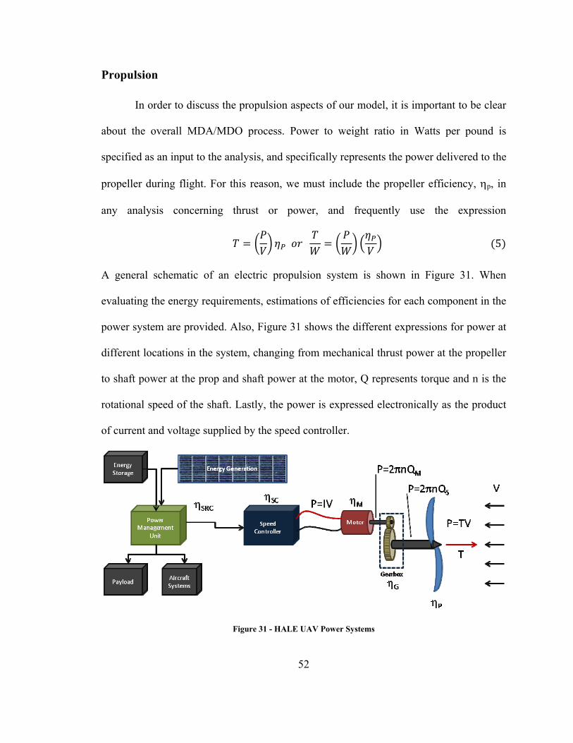
52
Propulsion
In order to discuss the propulsion aspects of our model, it is important to be clear
about the overall MDA/MDO process. Power to weight ratio in Watts per pound is
specified as an input to the analysis, and specifically represents the power delivered to the
propeller during flight. For this reason, we must include the propeller efficiency, ηp, in
any analysis concerning thrust or power, and frequently use the expression
5
A general schematic of an electric propulsion system is shown in Figure 31. When
evaluating the energy requirements, estimations of efficiencies for each component in the
power system are provided. Also, Figure 31 shows the different expressions for power at
different locations in the system, changing from mechanical thrust power at the propeller
to shaft power at the prop and shaft power at the motor, Q represents torque and n is the
rotational speed of the shaft. Lastly, the power is expressed electronically as the product
of current and voltage supplied by the speed controller.
Figure 31 - HALE UAV Power Systems

53
A description of the efficiencies is presented in Table 7, along with some assumed values
for the components, intended to be conservative.
Table 7 – General Power Train Efficiencies
Symbol Description Value
Propeller efficiency 0.80
Gearbox efficiency 0.95
Motor efficiency 0.90
Speed controller efficiency 0.90
Source efficiency (batt,fc, etc.) 0.90
Using a more flexible sizing method like the one given in [36] requires the
definition of several additional efficiency parameters. Also, more specific data is
available for several items in Table 7. Just as an example, the source efficiency in Table 7
of 90% may be reasonable, or even conservative for batteries, but if we decide to
implement fuel cells, the source efficiency drops to only 50%.
Table 8 - Specific Power Train Efficiencies [36]
Symbol Description Value
Battery efficiency 0.98
Fuel cell efficiency 0.50
Power management and distribution efficiency
0.97
Motor efficiency 0.97
Total power train efficiency is then calculated as the product of applicable
component efficiencies for the power system employed. There is a subtlety, however,
pertaining to energy processes within the MDA environment. As pointed out on the

54
previous page, when interested in the thrust available from the aircraft, a propeller
efficiency is already built into the equation. Consequently, the power requirement from
other modules like Mission Analysis describes what must be delivered to the propeller. It
follows that integrating that power over the mission time produces the energy required at
the propeller, ER. What this means is that the energy delivered by the Power Management
and Distribution (PMD) unit must exceed this value to account for power train
imperfections. Here we designate the energy output from the PMD as ES, or the required
total stored energy, given in (6)
∏ 6
where ηn is the efficiency of an energy component n in the power train, but does not
include propeller efficiency.
With regard to propeller efficiency, Table 7 lists it as a static value despite the fact
that for fixed-pitch propellers, as many HALE UAV platforms may well be, the
efficiency changes during flight. There are several reasons that this parameter (ηp) has
been implemented as such. First, considering the preliminary stages of design we are
operating in, propulsive sizing requires a scalable architecture. This means that rather
than selecting a specific propeller, we assume that if we use a reasonable efficiency value
then eventually a prop may be found to meet or exceed it. Second, the primary focus of
this effort is to investigate parametric changes and sensitivities. Accordingly, it is valid to
use a reasonably assumed value for ηp as long as we evaluate how changing the
assumption affects the resulting aircraft. This sensitivity study is presented in the Tool
Validation section.

55
Energy System Weights
With both energy system efficiencies and data from Mission Analysis, the MDA
environment has developed the total system energy storage requirement, ES, for a
mission. The final task for the energy and propulsions module, then, is to determine how
much the energy system must weigh. Energy system components can be broken up into
three categories. First, energy generation describes things like solar cells and supporting
infrastructure. Second, energy storage represents batteries, or fuel / fuel tanks if
applicable. Finally, energy conversion components are those that transform stored energy
into useful work. Energy conversion is where we classify fuel cells, Power Management
and Distribution units, and motors.
Weight of the energy generation system, essentially the solar panels and
equipment, is estimated based on the required solar coverage area. Information from
several sources concerning modern solar cells leads to an area density of the solar power
system, ρAsol = 0.11 pounds per square foot of solar area [46], [47].
Energy storage weight is developed from the total energy storage requirement, ES,
and information regarding the specific energy density of storage components. This
technology metric has been discussed previously for batteries, but if fuels are used with a
fuel-cell, the sizing methods of [36] provide applicable information, adapting an energy
density metric to scalable components like liquid Hydrogen tanks.
Energy conversion weights are built up from power density specifications rather
than energy density. For example, [36] claims advanced electric motor technology to be
capable of producing 3.4 kW/kg of motor weight (1.54 kW/lb). So calculating energy
conversion system weight involves connecting the total aircraft power requirement with a

56
summation of whichever energy conversion components are part of the system. When
evaluating Helios baselines, however, we know that each motor provided 1.5 kW of
power [21]. Therefore a general estimate for weight per motor is used based on
commercially available brushless DC motors of similar power. Total number of motors
may then be estimated from the maximum power per motor, the power to weight ratio of
the aircraft, and the gross weight.

57
Structures
Estimating structural weight is another highly important aspect of preliminary
design. Several methods for mass prediction are possible, involving varying levels of
sensitivity to configuration, validity, or computational simplicity. Standard methods
include using historical regressions of existing aircraft data to approximate weights of
components or subsystems. Specifically, [33] develops weights for elements of the
airframe like the spar, ribs, control surfaces, fuselage, et. al. as functions of the total
weight and wing geometry. One example of implementing these weight predictions is
given in [48]. For application to the work herein, there are several factors discouraging
the use of such methods. First, the methods in [33] were published in 1984, and therefore
the platforms that make up the regression models predate several key technology
demonstrators or recent design efforts. Also, investigating an unconventional
configuration like a pinned-segmented flying wing discourages use of such weight
models because it diverges from the aircraft basis for the regression. For this reason, a
bottom-up weight model is developed, relying strongly on a structural analysis of the
wing geometry.
There are several decisions that must be made prior to completing structural
analysis. Fundamentally, the purpose of our structures module is to design the spar cross
section to withstand a certain loading condition, and output the resulting spar weight. In
addition, the module will estimate a total wing structural weight. These tasks require
knowledge of the spar geometry, material properties, and desired factor of safety, as well
as loading information. The structural design of our HALE UAV will mimic that of the
NASA ERAST vehicles and Helios and is composed of a tubular spar cross section and a

58
non-stressed wing skin (Figure 32) [21], [49]. Likewise, wing structural material will be a
carbon fiber composite.
Figure 32 - Helios Wing Structural Arrangement [50]
Figure 33 shows the process for performing the wing structural analysis and
developing a weight estimate.
Figure 33 - Structural Analysis Process
First, the aerodynamic loading distribution is brought in from the Aero Loads module,
and when combined with the span loaded weights of other systems (motor, solar, energy

59
storage, etc..), a net loading distribution is available. Figure 34 shows a general spanwise
loading for the baseline single-segment wing configuration, major point loads represent
the locations of battery pods. The net loading is then integrated to produce shear and
bending moment distributions (Figure 35).
Figure 34 - General Spanwise Loading Distribution
Figure 35 - General Spanwise Shear and Moment Diagrams
0 50 100 150 200 250-50
-40
-30
-20
-10
0
10
20
30
40
50
<----root Half-span location tip---->
Load
(lb)
Net ForceLift ForceBattery WeightsEnginesSolar Panel SystemStructure
0 0.1 0.2 0.3 0.4 0.5 0.6 0.7 0.8 0.9 1-1500
-1000
-500
0
<----root Half-span location (%) tip---->
Shea
r (lb
)
0 0.1 0.2 0.3 0.4 0.5 0.6 0.7 0.8 0.9 1-10
-5
0x 104
<----root Half-span location (%) tip---->
Mom
ent (
ft-lb
)
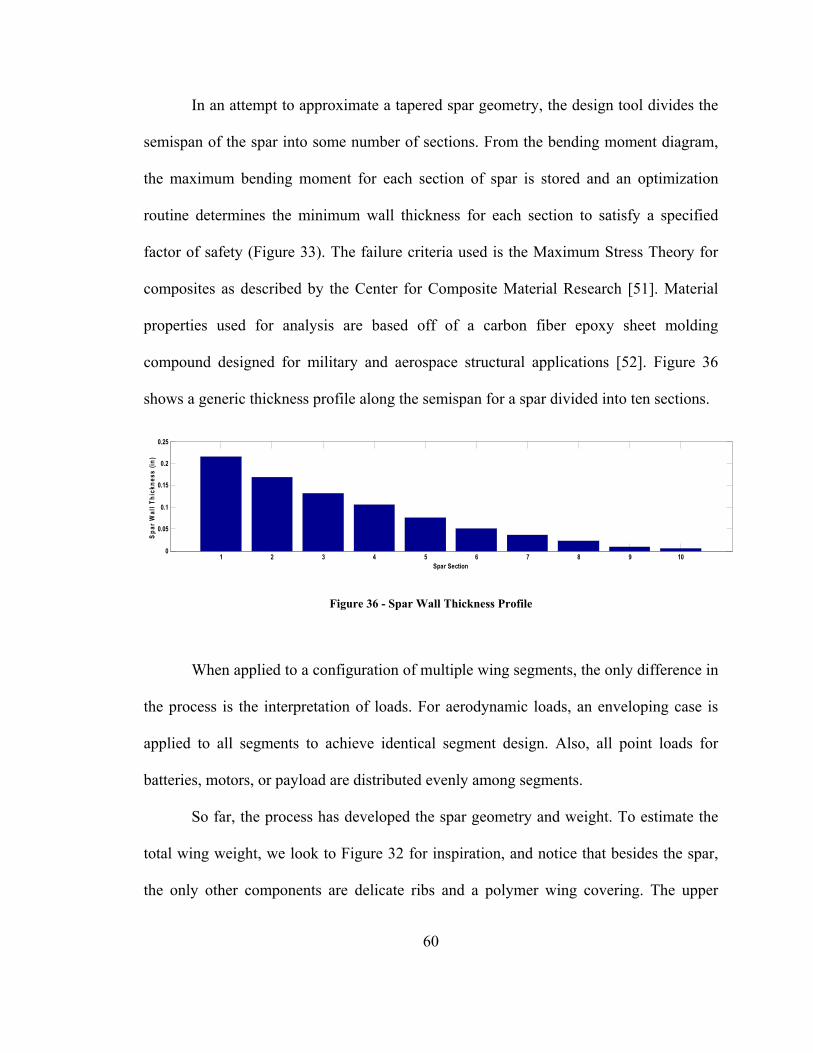
60
In an attempt to approximate a tapered spar geometry, the design tool divides the
semispan of the spar into some number of sections. From the bending moment diagram,
the maximum bending moment for each section of spar is stored and an optimization
routine determines the minimum wall thickness for each section to satisfy a specified
factor of safety (Figure 33). The failure criteria used is the Maximum Stress Theory for
composites as described by the Center for Composite Material Research [51]. Material
properties used for analysis are based off of a carbon fiber epoxy sheet molding
compound designed for military and aerospace structural applications [52]. Figure 36
shows a generic thickness profile along the semispan for a spar divided into ten sections.
Figure 36 - Spar Wall Thickness Profile
When applied to a configuration of multiple wing segments, the only difference in
the process is the interpretation of loads. For aerodynamic loads, an enveloping case is
applied to all segments to achieve identical segment design. Also, all point loads for
batteries, motors, or payload are distributed evenly among segments.
So far, the process has developed the spar geometry and weight. To estimate the
total wing weight, we look to Figure 32 for inspiration, and notice that besides the spar,
the only other components are delicate ribs and a polymer wing covering. The upper
1 2 3 4 5 6 7 8 9 100
0.05
0.1
0.15
0.2
0.25
Spar Section
Spar
Wal
l Thi
ckne
ss (i
n)

61
surface of the wing is occupied by solar panels, of which we estimate weight separately.
Currently, the total wing weight is estimated at 1.1 times the spar weight because of the
ultralight construction methods available.
Weights
The specifics concerning weight estimation for each contributing discipline have
been discussed in their sections above. Total weight, then, is computed as the sum of the
wing structure, tail structure (if applicable), energy storage, energy generation, propulsion
components, and payload weights. In finalizing weight statements for a variety of HALE
configurations, reference [49] mentions a 6% mounting and installation mass addition. To
account for additional miscellaneous items, a 5% margin is added onto our estimate for
the final gross weight. Component weight breakdowns and comparisons of results with
existing aircraft are presented in the Validation section.

62
Performance
Analysis of the flight performance of the aircraft is an integral part of flight
planning, mission analysis, and constraint analysis. As a module in the design
environment, the performance analysis is completed last. Structuring an N-squared
diagram or Design Structure Matrix (DSM) involves placing processes at the end if they
have no dependants [32], and the outputs of the performance analysis block are used only
for constraints in the optimizer. As previously mentioned, the mission analysis and flight
planning tasks involve some processes similar to those contained in the performance
module, but the application of the tasks is slightly different here. The main goal for flight
planning was to optimize flight CL at different stages for minimum energy or minimum
power. In the performance analysis block, the focus is on finding maximum capabilities
of the aircraft. Most important is an estimation of the absolute ceiling, maximum rate of
climb, best sustained turn radius, dash speed, and takeoff distance.
The central process for calculating performance is an excess power function based
on the fact that . Since we are dealing with propeller aircraft, this expression
should use power available rather than thrust available. Also, the routines are written
such that the weight of the aircraft is not necessary, using parameters like wing loading
and power to weight ratio. Lastly, it is desirable to express power in terms of Watts, so a
conversion factor is necessary. 0.73756 converts power from foot-pounds per
second into Watts. The resulting expression for excess power is given in equation 7.
2 7

63
Excess power from equation 5 is synonymous to the rate of climb of the aircraft at
the given speed and altitude, and we may approach the analysis from two perspectives. If
the aircraft size is not known, must be based on an assumed drag polar. This allows us
to evaluate point performance qualities of a scalable aircraft in terms of wing loading,
power to weight, aspect ratio, etc. Alternatively, if the size of the aircraft is determined,
reference and wetted areas are known and an accurate drag polar may be used to
determine the actual performance metrics.
Many times, point performance requirements, expressed as constraints, leave a
certain level of freedom open to the aircraft. For example, we may specify that the
aircraft must exhibit at least 300 feet per minute rate of climb at a certain altitude, but not
specify the speed at which it must occur. Reference [49] discusses some other
requirements including a dash speed necessary to overcome the worst case 99th percentile
winds aloft, a statistical value for wind speeds that are only exceeded 1% of the time. A
dash requirement may then be specified at either the cruise altitude or left free to be
satisfied at any altitude. When there is such a degree of freedom, the performance
calculations are subject to a minimization routine where the free variable like velocity or
altitude is determined for best performance. MATLAB’s fminbnd is generally what is
used in this case where single variable functions are minimized on a fixed interval. Note
that we usually want to maximize the quantity, so fminbnd applies a negative sign to the
function in question. Figure 37 shows the core of the performance analysis process
employed herein.

64
Figure 37 - Performance Analysis Process
Several performance charts are reproduced here in an effort to familiarize the
reader with low wing loading values and power expressed in Watts. These performance
calculations were completed with a simplified analytical drag polar and intend to
demonstrate the operation of the process in Figure 37. The first point performance metric
is the absolute ceiling, and constitutes one of the fundamental requirements or constraints
on our system. Figure 38 below confirms that the high altitudes of interest to a HALE
UAV drive the designs to aspect ratios on the order of 1 lb/ft2.
Figure 38 - Absolute Ceiling (kft)

65
With the areas of wing loading and power-to-weight favorable to high altitude
flight in mind, we see from Figure 39 that minimizing power that will allow a 100,000 ft
ceiling results in roughly 400 ft/min maximum rate of climb at sea level. Also, for the
design space shown, maximum rate of climb is much more dependent on power-to-
weight than on wing loading.
Figure 39 - Max Rate of Climb (ft/min)
When operating in the integrated MDO environment, this performance code will
have more information available, like aircraft weight, detailed drag polars, and one
specific design point wing loading and power-to-weight. These extra details take the
place of the assumptions made to create the plots seen above, and rather than plotting
over the whole design space, required performance metrics are calculated for just one
point.

66
The Integrated Environment
Assembling the individual disciplines and analysis/design modules discussed
above finally provides the multidisciplinary analysis and design environment that we
desire. Figure 40 shows a generalized schematic of how the disciplines communicate, and
how the parameters of this environment may be controlled with an optimization routine.
Figure 40 – Final MDO Tool Schematic
67
IV. TOOL VALIDATION
For a design tool to be at all useful, it must be checked to ensure some level of
accuracy. Here, an attempt is made to explore the basic behavior of the MDA system and
perform initial tests for sensitivities, and optimizer integration. The basic configuration
modeled for the validation cases is a flying wing aircraft utilizing solar energy generation
and advanced battery energy storage. This configuration allows comparison of results
with the Helios Prototype aircraft. Several variants of Helios were flown, ranging from
initial checkout flights powered entirely with batteries to the HP01 aircraft that reached
record altitude to finally the ill-fated HP03 fuel cell powered long endurance
configuration.
It is important to note that the goal for this study is to provide a design
environment to support investigation of incremental benefits and sensitivities of various
HALE UAV concepts. These parametric studies rely on tools that correctly model certain
physical responses to changing inputs, but the focus is centered more on capturing the
delta than finding exactly the quantity. Consequently, the purpose of a validation study is
to ensure that the results are within a reasonable order of accuracy and calibrate areas of
error. If the user determines that the MDA results are unacceptable, the task of
identifying the suspect disciplines and replacing the module with one of greater accuracy
is not a difficult one. Unfortunately, commonly available technical information for Helios
is not highly detailed (Table 9), but should serve our purpose for this study. Building an
approximation of Helios in our MDA environment involves specifying certain
configuration inputs (Table 10) and evaluating the resulting aircraft.
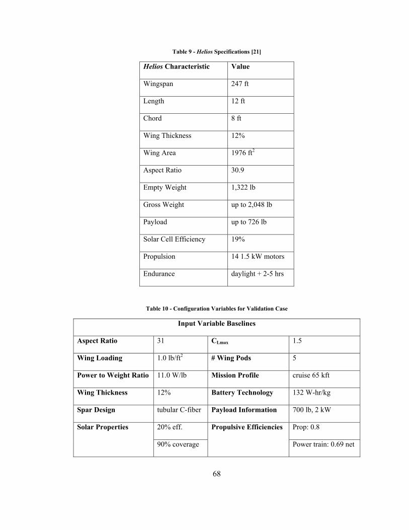
68
Table 9 - Helios Specifications [21]
Helios Characteristic Value
Wingspan 247 ft
Length 12 ft
Chord 8 ft
Wing Thickness 12%
Wing Area 1976 ft2
Aspect Ratio 30.9
Empty Weight 1,322 lb
Gross Weight up to 2,048 lb
Payload up to 726 lb
Solar Cell Efficiency 19%
Propulsion 14 1.5 kW motors
Endurance daylight + 2-5 hrs
Table 10 - Configuration Variables for Validation Case
Input Variable Baselines
Aspect Ratio 31 CLmax 1.5
Wing Loading 1.0 lb/ft2 # Wing Pods 5
Power to Weight Ratio 11.0 W/lb Mission Profile cruise 65 kft
Wing Thickness 12% Battery Technology 132 W-hr/kg
Spar Design tubular C-fiber Payload Information 700 lb, 2 kW
Solar Properties 20% eff. Propulsive Efficiencies Prop: 0.8
90% coverage Power train: 0.69 net

69
Notice that several required input variables in Table 10 are not directly defined in
the available information, specifically CLmax and the propulsive efficiencies. Also, the
extra flight time and mission profile information may vary flight-to-flight with Helios.
These characteristics are major design drivers, so for the first analysis case, some
baseline values are assumed and a sensitivity analysis will be presented. Table 11 shows
the analysis results for a baseline approximation of the Helios platform.
Table 11 - Baseline Validation Results
Characteristic Helios MDA tool Difference % Error
Wingspan (ft) 247 258.08 -11.08 4.49%
Chord (ft) 8 8.33 -0.33 4.06%
Wing Area (ft2) 1976 2148.55 -172.55 8.73%
# Motors 14 16 -2 14.29%
Gross Weight (lbs) 2048 2148.43 -100.43 4.90%
Error circa 5% on gross weight is encouraging, but it is prudent to investigate a bit
farther. As mentioned earlier in the paper, the weight of the aircraft in the MDA
environment is broken into payload, energy generation and storage, wing/tail structure,
and propulsion components. Figure 41 shows the breakdown of gross weight by category
for the baseline MDA, and highlights a slight discrepancy compared to our validation
aircraft. The empty weight of Helios was quoted at 1,322 lbs, and the baseline analysis
given here shows an empty weight of 800 pounds. Differences here are heavily dependent
on the spanwise loading distribution, of which limited information is available for HP01,
as well as on the battery scheme included. There are several methods of accounting for

70
differences in cases like this such as implementing a correlation factor, possibly in the
form of increasing the 5% miscellaneous item weight.
Figure 41 - Baseline Weight Breakdown
Before making adjustment to the tool, we must consider that some of the
information that Figure 41 is based on was assumed. Also, recall that the focus here is
primarily to evaluate the trends intrinsic to the design tool as long as it provides generally
accurate results. Accordingly, an effort is made here to investigate the sensitivities to
some of the key configuration inputs, specifically the ones where limited information is
available and assumptions are necessary. For the following parametric study, a baseline
configuration is defined by Table 10 and certain values are perturbed one at a time.
Payload700 Battery
655
Solar215
Wing316
Motors160
0
100
200
300
400
500
600
700
800
Wei
ght (
lbs)

71
Maximum Lift Coefficient Response
A nominal CLmax of 1.5 was used to obtain the results of Table 11 and Figure 41.
In general, the maximum lift coefficient of a HALE aircraft has a much greater effect on
the mission performance than it does for conventional aircraft. The combination of a high
aspect ratio wing and an extremely low wing loading decrease the induced drag of the
aircraft drastically, causing the airspeed for minimum power to drop. In many cases, this
minimum power flight condition may be below the stall speed of the planform. Figure 42
shows how this best power flight condition changes with increasing aspect ratio for a
generic HALE type of aircraft [53].
Figure 42 - CL for Minimum Power
It is clear that the flight planning and mission analysis of the vehicle desire a high lift
coefficient, and this CLmax should have a noticeable effect on the energy requirement and
therefore weight of the resulting aircraft. Figure 43 shows the results of changes in
maximum lift coefficient applied to a Helios – based design.

72
Figure 43 - Response to CLmax Perturbation
When examining these results, one must keep in mind that the other pre-specified
characteristics of the aircraft have not changed, most importantly the wing loading is a set
value between the three cases of Figure 43. Also worth noting is that during flight
planning and mission analysis, the lower bound for choosing a flight condition is 1.2
times Vstall, forcing the aircraft farther from the optimal point. What we see is that
increasing the maximum lift coefficient does in fact allow the aircraft to operate at a more
favorable CL as evidenced by the reduction in energy component weights. Also, the fact
that the wing structural weight is sensitive to CLmax confirms that some of the finer
interdisciplinary connections are working well. Specifically, the incremental increase in
CLmax has decreased the energy requirement, thereby decreasing the weight of the
batteries for after-hours flight. The savings in battery weight translates to a slightly
smaller wing for a given wing loading, reducing the weight of the solar power system and
altering the load distribution of the wing resulting in an overall decrease in gross weight.
700 700 700
688 655 634
222 215 212
328 316 311
180 160 160
0
500
1000
1500
2000
2500
CLmax 1.4 Baseline CLmax 1.5 CLmax 1.6
Wei
ght (
lbs) Motors
WingSolarBatteryPayload Weight
Baseline CLmax 1.5
CLmax 1.4 CLmax 1.6

73
Moving the other direction with CLmax the design environment again exhibits
expected behavior. Lower maximum lift coefficient forces our operating conditions off
optimum and increases the energy requirement and gross weight of the aircraft. Also, the
added power requirement exceeded the maximum available from the motors on the
baseline, so two were added to maintain symmetry. For this design study, a 6.7% increase
in CLmax results in 1.4% decrease in gross weight while decreasing the max lift coefficient
the same amount increases the gross weight by 3.6%.
Propeller Efficiency
DARPA’s Broad Agency Announcement for the Vulture Program specifically
calls out “extremely efficient propulsion systems” as a potential area for funded
development [5]. Helios included composite propellers designed to exhibit laminar flow
at high altitudes for increased efficiency. In addition, the NASA Dryden Flight Research
Center is developing a testing capability for subsonic small general aviation and UAV
aircraft research, including topics like variable pitch props and real-time efficiency
control loops [54]. From the standpoint of the design environment developed here, it is
possible to integrate performance maps for a specific prop if desired, but if no
information is available for the propeller, a constant prop efficiency is used. As with
CLmax information, detailed data concerning the Helios propellers is limited.
Propeller efficiency was briefly discussed in the propulsion section earlier, but it
boils down to the fact that there is a certain mechanical power required for flight, and a
higher ηp means less energy is wasted during conversions in Figure 31. Because this

74
value is assumed during the validation analysis, again we want to evaluate how much a
change in the input affects the output of the system.
Figure 44 - Response to ηP Perturbation
Again, the system responds as we expect, increasing efficiency drives energy
requirements down resulting in overall weight reduction. Here, a 12.5% increase in
efficiency gives 3.4% decrease in gross weight while decreasing the efficiency the same
amount incurs a weight penalty of 6.7%. Similar to the maximum lift coefficient
sensitivity, given a certain change, the systems responds more to a detrimental delta than
a beneficial one.
700 700 700
734 655 605
229215 207
340316 304
180160 160
0
500
1000
1500
2000
2500
Wei
ght (
lbs) Motors
WingSolarBatteryPayload Weight
ηP 0.7 ηP 0.9 Baseline ηP 0.8 ηP 0.7

75
Target Altitude
Ultimately, Helios was a prototype technology demonstrator with the eventual
goal of demonstrating sustained flight to support any number of HALE UAV conops. A
successful platform would ideally climb to its operational or target altitude, and either
cruise or loiter for as long as possible. Though in practice and during the test flights the
Helios aircraft may have deviated from this mission profile, the standard mission shown
in Figure 11 is used as the design mission in the MDO tool. Specific data covering record
setting flight profiles is not included and the difference in mission requirements may
account for some discrepancies. Because there are many possible payloads and mission
profiles to choose from, we must explore the performance of the aircraft for different
target altitudes. Here, a target altitude is taken to mean the location of the main mission
operation, and is separate from the ceiling of the aircraft, which may be much higher.
Conceptually, climbing to a higher operating altitude will require more energy,
and should impose a weight penalty on the aircraft. Figure 45 confirms additional weight
for higher altitude cruise conditions, but careful interpretation is necessary. Recall that
Helios, weighing in at 2048 pounds or less was able to set flight altitude records in the
mid-90 kft range. The difference is that the aircraft in the MDO environment is being
sized to complete a day-long mission at that altitude and continue 2 hours after sunset at
the cruise condition before beginning a descent. During the record setting altitude flights,
Helios reached an altitude of 96,883 feet, but only sustained flight above the 96,000 foot
mark for 40 minutes.

76
Figure 45 - Response to Target Altitude Perturbation
Once again, the penalty incurred for a change in input is greater than the benefit
from the same change in a positive direction. Here, target altitude is altered 23.1% from
its baseline value, and the aircraft grows 21.1% to perform the high altitude loiter
compared to a 6.1% weight savings for operating at the lower altitude.
Night Flight and Battery Requirement
One of the largest determinants of the final weight of our HALE aircraft is the
requirement for stored on-board energy. Most of the literature concerning the Helios
Prototype mentions that it was capable of somewhere between one and five hours of
operation after sundown [20], [21], [44]. The NASA spec sheet for Helios states that
lithium batteries were used, but minimal information is available concerning mission
700 700 700
566 655927
201 215
260294
316
391160
160
200
0
500
1000
1500
2000
2500
3000
50 kft cruise Baseline 65 kft cruise
80 kft cruise
Wei
ght (
lbs) Motors
WingSolarBatteryPayload Weight

77
specifics like at what flight condition the aircraft operated during the 2-5 additional
hours. There are several methods of accounting for an unknown factor like this after-dark
flight capability in the design environment contained herein. First, the battery technology
factor is scaled back to where state of the art batteries were in the late 1990’s. In terms of
specific energy density, advanced lithium-ion batteries may have achieved somewhere on
the order of 130 Watt-hours per kilogram (roughly 60 Watt-hours per pound). Second, if
the actual weight of the battery system implemented in Helios is known, it may be
supplied to the design environment, producing the after-sunset flight capability an output.
Alternatively, we may set the minimum required extra flight time as an input and the
energy analysis modules cooperate with mission analysis to find the resulting battery
weight necessary to continue the mission that long. Once again, as implemented, the extra
time is on-station cruise or loiter condition flight, and the aircraft may begin descent
afterwards.
For the baseline validation case, an additional flight time requirement of two
hours was imposed. Of course we must evaluate how sensitive the resulting design is to
this requirement. Figure 46 shows the aircraft gross weight sensitivity to changing night
flight times. Here we see how drastically the additional endurance requirement affects the
system. In addition, updating the battery energy density from the Lithium-ion technology
to the current state of the art Lithium-Sulfur (Li-S) batteries increases the amount of
energy storage per unit weight threefold. Figure 47 shows the resulting weight benefits.
The baseline Lithium-ion aircraft with the ability to cruise 2 hours after sundown can
save nearly 30% of its gross weight if upgraded to Lithium Sulfur technology.
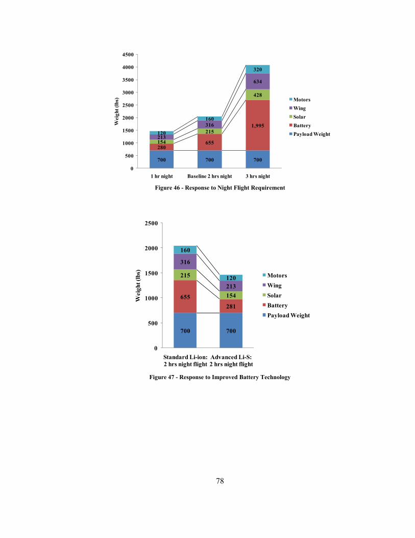
78
Figure 46 - Response to Night Flight Requirement
Figure 47 - Response to Improved Battery Technology
700 700 700
280655
1,995
154
215
428
213
316
634
120
160
320
0
500
1000
1500
2000
2500
3000
3500
4000
4500
1 hr night Baseline 2 hrs night 3 hrs night
Wei
ght (
lbs) Motors
WingSolarBatteryPayload Weight
700 700
655281
215
154
316
213
160
120
0
500
1000
1500
2000
2500
Standard Li-ion: 2 hrs night flight
Advanced Li-S: 2 hrs night flight
Wei
ght (
lbs) Motors
WingSolarBatteryPayload Weight

79
V. OPTIMIZING BASELINE ARCHITECTURE
Evaluating benefits of the pinned wing concept can only be completed if there is a
baseline capability to compare against. The first step is developing this basis for
comparison is to build on the Helios validation case and introduce some extra degrees of
freedom into the design. Progressively adding more design variables to an optimization
routine will eventually build up the optimal baseline conventional HALE configurations
that we need. First, the implementation of the Helios-style baseline aircraft described
previously will be allowed to choose its own wing loading and power to weight ratio. The
objective of the optimizer is to minimize the gross weight of the aircraft, and at first the
only constraints specified are the convergence of weight, absolute ceiling of 100 kft, and
a wingspan less than 300 ft. After solutions are found with only the two design variables,
the same optimization is completed with the addition of aspect ratio as a free variable. At
this point we may either continue to add more design variables to the optimizer for the
validation mission concept of limited after-dark flight, or we may add the constraint for
repeatable day/night energy cycles. Results for both avenues will be presented. Lastly,
with the 24 hour constraint in place, the remaining design variables are unleashed and a
full optimal solution to the two conventional mission concepts is sought. Please note that
describing an aircraft as conventional here means that it is a one piece cantilevered or
span loaded wing, contrasting the unconventional implementation of pinned wings. This
process of building baseline optimal configurations is illustrated in Figure 48.

80
Analysis
All inputs and configuration parameters are pre-set
MDO Stage I
Mission: Daytime PlusTechnology: HeliosDesign Variables:
* Wing loading* Power to weight
MDO Stage II
Mission: Daytime PlusTechnology: HeliosDesign Variables:
* Aspect ratio* Wing loading* Power to weight
MDO Stage III
MDO Stage III(a)
Mission: Daytime PlusTechnology: HeliosDesign Variables:
* Aspect ratio* Wing loading* Power to weight* Wing thickness
(Baseline 1)
MDO Stage III(b)
Mission: Long EnduranceTechnology: State of the artDesign Variables:
* Aspect ratio* Wing loading* Power to weight* Wing thickness
MDO Stage IV
Mission: Long EnduranceTechnology: State of the artDesign Variables:
* Aspect ratio* Wing loading* Power to weight* Wing thickness* Solar cell area
(Baseline 2)
Figure 48 - Optimal Baseline Development Procedure

81
Stage I: Power and Wing Loading as Design Variables
For the given Helios aspect ratio, wing thickness, technology level, and other
characteristics of the baseline in Table 10, we now explore a design space of wing
loading and power levels. Performing MDO on a complex system that uses a variety of
analysis codes and table lookups tends to result in an unfavorable response surface for the
objective function. We may expect local minima, or difficulty finding a feasible point.
Indeed, choosing a feasible starting point is nearly impossible because of the Partial
Optimizer Based Decomposition of the feedback links. Since the convergence of the
design is a constraint imposed on the system, supplying a feasible point would mean that
we would have already solved the system. In addition to the issue of local minima, the
constraints on weight convergence pose another problem for finding the true optimum.
Once the optimizer is able to make its way to a point where all the constraints are
satisfied, where normally we would search for other feasible points that improve our
objective, the optimizer for this effort has difficulty perturbing from one feasible point
and finding another.
In order to explore as much of the design space as possible and find the overall
best solution, the optimization is run many times for a variety of different starting points.
The start point for each run is determined randomly based on a reasonable interval for
each design variable. Table 12 shows the best results for the first stage of building an
optimum conventional HALE UAV.

82
Table 12 - Stage I Baseline Optimization Summary
Design Variable Start Point Lower Bound Upper Bound Optimum
Wing Loading (lb/ft2) 0.815 0.5 5.0 0.875
Power to Weight (W/lb) 14.13 0.6 60.0 7.44
Progress of the design variables in this optimization run is tracked in Figure 49. As
noted previously, the parameters of the optimization are scaled to be of the same order of
magnitude, so the vertical axis in Figure 49 is scaled differently depending on which
variable is considered. The scaling factors for this diagram are as follows:
• Gross Weight: scale up by 1000
• Wing Weight: scale up by 100
• Wing Loading: scale is 1 to 1
• Power to Weight Ratio: scale up by 10
Figure 49 - Scaled Design Variable History
1 2 3 4 5 6 70.5
1
1.5
2
2.5
3
Iteration Number

83
Checking constraint violation helps to illustrate why some selections are made for
design variables, Figure 50 shows the objective function history with points colored
according to constraint violation. Green points designate that that the maximum
constraint violation at that iteration was less than the specified tolerance.
Figure 50 - Stage I Objective Function History
The results of this initial optimization case correlate well with the actual aircraft,
as the wing loading for Helios varies by mission but is in the range of 0.8 to 1.1 pounds
per square foot [21]. When compared with our baseline analysis (see Figure 51) the effect
of decreased wing loading and power to weight is a decrease in weight because less
energy is required for flight.
1 2 3 4 5 6 71500
1600
1700
1800
1900
2000
2100
2200
2300
2400
Iterations
Wto

84
Figure 51 - Stage I Optimization Component Weights
Stage II: Adding Aspect Ratio as a Design Variable
The next step toward an optimal baseline configuration is the introduction of
aspect ratio as a design variable. Here, again, constraints are imposed for absolute ceiling,
wingspan, and design convergence, and the same method of using randomly generated
start points is employed. Table 13 summarizes the design variable optimal values.
Table 13 - Stage II Optimization Summary
Design Variable Start Point Lower Bound Upper Bound Optimum
Aspect Ratio 38.63 10 60 32.73
Wing Loading (lb/ft2) 1.04 0.5 5.0 0.854
Power to Weight (W/lb) 16.45 0.6 60.0 7.55
Design variable history is included in Figure 52 and shows that the additional
design variable has increased the number of iterations required. Also, the behavior
700 700
655 583
215 227
316266
160120
0
500
1000
1500
2000
2500
Helios Baseline Optimal Wing Loading and
Power
Wei
ght (
lbs)
MotorsWingSolarBatteryPayload Weight

85
exhibited here of making large initial steps and then slowly proceeding with minute
changes is common for these optimization runs. As before, the variables are appropriately
scaled in the MDO environment.
Figure 52 - Stage II Scaled Design Variable History
In this case, as the design variables make small perturbations to find new line
search directions, Figure 53 shows that the constraints are not all met until the final
iteration. Results of this optimization are that a slightly higher aspect ratio and lower
wing loading may contribute a slight weight savings, 0.7% over the Stage I optimum but
totaling 8% lower weight than the baseline (see Figure 54). Also, an interesting trend is
shown in Figure 54 concerning wing weight. With a decreased battery and engine weight,
the point loads along the span decrease, and the loss of their benefit for load alleviation
necessitates a slightly heavier wing structure to keep a positive margin of safety.
0 5 10 15 20 25 300
0.5
1
1.5
2
2.5
3
3.5
4
Iteration Number
Wto e3Wwing e2AR e1WoS e0PoW e1

86
Figure 53 - Stage II Objective Function History
Figure 54 - Comparison of Optimal Weight Breakdowns
If we examine the actual constraint history (Figure 55) we see that the optimizer
was close to a solution by the fifth iteration, and altering the tolerance on constraint
violation may allow for decreased run times.
0 5 10 15 20 25 301600
1700
1800
1900
2000
2100
2200
2300
Iterations
Wto
700 700 700
655 583 565
215 227 231
316266 286
160120 100
0
500
1000
1500
2000
2500
Helios Baseline Optimal Wing Loading and
Power
Optimal Wing Loading, Power,
and AR
Wei
ght (
lbs)
MotorsWingSolarBatteryPayload

87
Figure 55 - Maximum Constraint Violation History
Stage III a: Full Optimization of “Daytime Plus” Mission
The final parameter to include in the optimization of the conventional aircraft
platform covered here is the wing thickness. Up to this point, a 12% thick airfoil was
included in the model because that is what the Helios Prototype employs. Changing the
thickness of the airfoil should affect the mission analysis from a drag perspective, but the
most drastic changes will most likely be seen in structural weight. Larger thickness
allows for a larger spar cross section and thinner walls. Table 14 shows the design
variable information, again with randomly generated start points. Wing thickness in this
optimization has run into the upper bound, confirming that spar structural weight benefits
from the increased thickness. Optimum values for the other variables have also changed,
with the increased thickness allowing a slightly higher aspect ratio than previous runs.
0 5 10 15 20 25 300
0.2
0.4
0.6
0.8
1
1.2
1.4
Iterations
Con
stra
int V
iola
tion
y

88
Table 14 - Stage III(a) Optimization Summary
Design Variable Start Point Lower Bound Upper Bound Optimum
Aspect Ratio 29.84 10 60 37.62
Wing Loading (lb/ft2) 1.16 0.5 5.0 0.826
Power to Weight (W/lb) 11.96 0.6 60.0 7.28
Wing Thickness (%) 15.73 10.0 30.0 30.0
Progression of the design variables toward the optimum is displayed below in Figure 56,
again scaled appropriately so that the gold line representing thickness to chord ratio ends
at a value of 3 but is implemented as 30% or 0.3 in the actual MDO environment.
Figure 56 - Stage III(a) Design Variable History
As before, Figure 57 below charts the result of each line search, and the objective
function value is tracked during optimization. Figure 57 shows that it is possible for the
optimizer to perturb the first feasible point that it finds, and will sometimes violate
constraints while searching for the optimum.
0 5 10 15 200.5
1
1.5
2
2.5
3
3.5
4
Iteration Number
Wto e3Wwing e2AR e1WoS e0PoW e1t/c e-1

89
Figure 57 - Stage III(a) Objective Value History
The resulting weight breakdown for this full optimization of a limited endurance
Helios proxy aircraft is shown compared to previous stage optima in Figure 58. The
majority of mass categories for this case are quite similar to previous runs except when it
comes to wing structural weight.
Figure 58 - Progression of Optimal Weight Breakdowns
0 2 4 6 8 10 12 14 161700
1750
1800
1850
1900
1950
2000
2050
2100
Iterations
Wto
700 700 700 700
655 583 565 543
215 227 231 215
316 266 286135
160120 100
100
0
500
1000
1500
2000
2500
Helios Baseline
Optimal Wing
Loading and Power
Optimal Wing
Loading, Power, and
AR
Optimal Wing
Loading, Power, AR,
and t/c
Wei
ght (
lbs)
MotorsWingSolarBatteryPayload Weight

90
With a 30% thick airfoil, the spar weight may be reduced by 53% over the 12% thick
airfoil of the previous case. In total, there is a 17.3% gross weight reduction from the
initial baseline to the current optimal configuration.
Because the structural weight of the aircraft shows such a strong response to wing
thickness, a few more details about each configuration are presented here. As previously
noted, the spar is designed with a tubular cross section and is broken up into some
number of sections. Maximum loading conditions are developed for each region of the
spar and the wall thickness of each is individually minimized to meet a given factor of
safety. For the MDO at hand, it is assumed that advanced composite construction
techniques are used and that in reality the aircraft spar would exhibit a continuous
thickness distribution. Accordingly, the spar of the baseline aircraft is divided into 10
sections for all MDO discussed in this paper. Figure 59 shows the discrete spanwise wall
thickness profile for two aircraft configurations. Spar sections are numbered from aircraft
centerline to wingtip. The blue bars in Figure 59 come from the baseline Helios proxy
case, while the green is the most recent optimum configuration. Stage I and II optima fall
in between the two cases shown.
Figure 59 - Spar Design for Two Configurations
12% Wing Thickness
30% Wing Thickness

91
Up to this point, we have focused on aircraft weight when comparing each
successive optima. The progression has brought us to the stage where we have found an
optimal baseline configuration from a design space with an acceptable degree of freedom,
or number of design variables. Before moving on, however, there are other characteristics
of each of these optima that have not yet been highlighted or compared to the original
baseline design. A cross section of aircraft characteristics is included below (Table 15).
Table 15 - Optimization Data Summary
The aircraft configuration of the rightmost column of Table 15 represents the Proven
Technology Medium Endurance Baseline aircraft for this study.
Helios Baseline Proxy Stage I Stage II Stage III(a)
Gross Weight (lb) 2048.00 2148.42 1990.13 1976.48 1776.90
Aspect Ratio 31.00 31.00 31.00 32.73 37.62
Wing Loading (lb/ft2) 0.8 - 1.1 1.00 0.87 0.85 0.83
Power to Weight 11.00 11.00 7.93 7.55 7.28
Sref 1976.00 2148.51 2267.91 2315.56 2150.66
Wingspan 247.00 258.08 265.15 275.31 284.43
Chord 8.00 8.33 8.55 8.41 7.56
Wing Thickness 12% 12% 12% 12% 30%
Takeoff Distance 71.04 66.44 65.67 64.57
Max Climb Rate 359.82 253.52 241.73 234.41
# Motors 14 16 12 10 10

92
Stage III b: Four Variable Optimization of Long Endurance Baseline
The third stage of progressively adding design variables to the MDO is divided
here to allow the exploration of a long endurance configuration. From the outset of this
project the two inspiring platforms were the Helios Prototype and the Broad Agency
Announcement for Vulture. If we are to design and optimize a pinned wing aircraft for
sustainable day/night operation, we must develop an appropriate optimal baseline
configuration as a standard. Stage III(a) delves as far into the battery powered Helios
aircraft as we can, but never attempted to surpass the couple of hours of night flight that
the aircraft demonstrated. Stage III(b) includes up to the wing thickness to the set of
design variables, but also imposes the constraint for a sustainable regenerative energy
balance. Also, several key technology factors are upgraded to current or projected near-
term values, including involving new power-system data given in [36]. Presented at the
2009 CAFE Foundation Electric Aircraft Symposium, the approach to sizing power- or
energy-system components includes data concerning power train efficiencies and electric
motor power densities. Other technology improvements are increased solar cell efficiency
from 20% to 30% and upping the energy density of the batteries from 130 to 400 Watt
hours per kilogram. The 400 W-hr/kg mark is based on Lithium-Sulfur batteries currently
entering the market, but advanced nano-wire Lithium-polymer batteries may soon reach
upwards of 700 W-hr/kg [36], [55].
Original technology and configuration definition parameters (Table 10) are
updated for this Advanced Technology Long Endurance Baseline (ATLEB) and
summarized below in Table 16.

93
Table 16 - Parameters Defining the Long Endurance Baseline
Advanced Technology Long Endurance Configuration Inputs
Mission Profile cruise 65 kft CLmax 1.5
Battery Technology 400 W-hr/kg # Wing Pods 5
Spar Design tubular C-fiber Payload 700 lb, 2 kW
Solar Properties 30% eff. Propulsive Efficiencies
Prop: 0.8
90% coverage Power train: 0.92 net
Recall from Figure 46 that when determining the system sensitivity to battery
powered flight requirements, an increase from 2 hours to 3 hours elicited an enormous
response, effectively doubling the aircraft weight. That result discourages the idea of a
solar-battery regenerative aircraft achieving continuous operation, but fortunately the
design environment was approximating 15 year old technology. With the updates listed in
Table 16, the optimization for a long endurance mission is completed and described
below (Table 17). As before, the best solution drives to the upper bound of wing
thickness, and the aspect ratio is in the high 30’s.
Table 17 - Stage III(b) Optimization Summary
Design Variable Start Point Lower Bound Upper Bound Optimum
Aspect Ratio 34.82 10 60 36.95
Wing Loading (lb/ft2) 0.86 0.5 5.0 0.77
Power to Weight (W/lb) 13.89 1.0 60.0 7.07
Wing Thickness (%) 11.13 8.0 30.0 30.0

94
Plots of design variable and objective function values are not outstanding for this
case compared to others. Figure 60 compares the resulting aircraft weight breakdown to
those previously developed. Notable results are that the increases in technology have
resulted in an aircraft that carries only slightly more batteries than the original limited-
endurance baseline, and that the total weight is just 5% higher than the optimized solution
to the Helios proxy.
Figure 60 - Weight Breakdown for the ATLEB Compared to Earlier Results
One further note concerning the Stage III(b) optimization case is that the three
inequality constraints mentioned in Table 5 are all active at the solution. The wingspan at
this optimum is 300 ft, the absolute ceiling is 100,036 ft, and the batteries included store
just enough energy to reach the time after sunrise when solar power is high enough to
power the plane. Though earlier optimizations involved an active ceiling constraint, this
is the first to push all the way to the upper bound of wingspan. The reason is that
strenuous mission requirements here cause the airplane to desire low wing loading and
high aspect ratio as energy storage penalties outweigh structural ones.
700 700 700
655 543 679
215215
243
316
135142
160
100
8
0
500
1000
1500
2000
2500
Helios Baseline Stage III(a) Stage III(b)
Wei
ght (
lbs) Motors
WingSolarBatteryPayload Weight
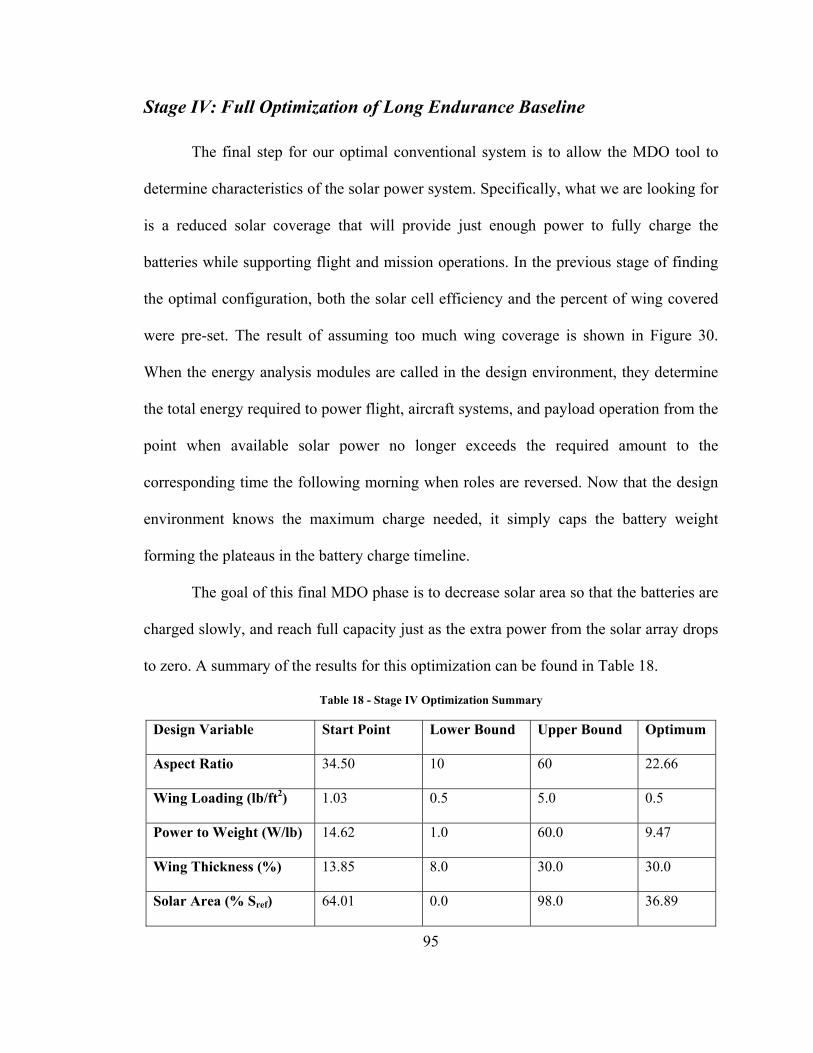
95
Stage IV: Full Optimization of Long Endurance Baseline
The final step for our optimal conventional system is to allow the MDO tool to
determine characteristics of the solar power system. Specifically, what we are looking for
is a reduced solar coverage that will provide just enough power to fully charge the
batteries while supporting flight and mission operations. In the previous stage of finding
the optimal configuration, both the solar cell efficiency and the percent of wing covered
were pre-set. The result of assuming too much wing coverage is shown in Figure 30.
When the energy analysis modules are called in the design environment, they determine
the total energy required to power flight, aircraft systems, and payload operation from the
point when available solar power no longer exceeds the required amount to the
corresponding time the following morning when roles are reversed. Now that the design
environment knows the maximum charge needed, it simply caps the battery weight
forming the plateaus in the battery charge timeline.
The goal of this final MDO phase is to decrease solar area so that the batteries are
charged slowly, and reach full capacity just as the extra power from the solar array drops
to zero. A summary of the results for this optimization can be found in Table 18.
Table 18 - Stage IV Optimization Summary
Design Variable Start Point Lower Bound Upper Bound Optimum
Aspect Ratio 34.50 10 60 22.66
Wing Loading (lb/ft2) 1.03 0.5 5.0 0.5
Power to Weight (W/lb) 14.62 1.0 60.0 9.47
Wing Thickness (%) 13.85 8.0 30.0 30.0
Solar Area (% Sref) 64.01 0.0 98.0 36.89

96
Again, for this optimization, the wingspan constraint is active, but there are
several aspects of these results that are suspect. First, the trend that we have observed up
till now of increasing aspect ratio has reversed to a value lower than the initial baseline.
Second, the wing loading design variable is at its lower bound, which in its own right is
not necessarily alarming, but in the context that we have not seen that behavior before
from the optimization cases it may be an area to investigate. In addition, we see in Figure
61 that during the third iteration the wing loading jumped to its lower bound and did not
visibly move for the remainder of the operation.
Figure 61 - Stage IV Design Variable History
Another area of question is that the power to weight ratio at the optimum has
increased from what was previously a steady and predictable value. Because of the jump
in power to weight, the ceiling of this configuration is 106,384 ft. It seems that the
appropriate action of the optimizer would have been to decrease the power to weight ratio
of the aircraft to reduce weight and remove the excess ceiling margin.
0 5 10 15 200
0.5
1
1.5
2
2.5
3
3.5
4
Iteration Number
Wto e3Wwing e2AR e1WoS e0PoW e1t/c e-1Percent Solar

ai
in
pr
bu
fu
at
th
co
ev
co
si
The m
ircraft gross
ncreased ove
Logic
revious stag
ut with a dec
unction resp
ttempt to fin
he process an
onfiguration
valuate the b
onfiguration
ignificant ev
most incrimin
s weight. Fig
er the previo
Figure
cally it seem
ge, remove a
creased sola
ponse surfac
nd the overal
nd selecting
n found from
benefit of im
n, we may s
vidence that
nating result
gure 62 sho
us stage resu
62 - Compariso
ms that we sh
a portion of
ar power syst
ce stifling ou
ll optimum b
the best resu
m a selectio
mplementing
simply selec
t the Stage
97
t, however, i
ows that the
ult.
on of Stage IV W
hould be abl
solar panels
tem weight.
ur optimizat
by choosing
ult among th
on ten rando
an ideal sola
ct appropriat
IV result in
is the actual
e required ba
Weight to Previ
le to take th
and have n
This is a pri
tion routine.
a random se
hem. Table 1
omized stari
ar arrangem
te starting p
n Table 18 i
objective fu
attery weigh
ious Optima
he optimum
nearly the sam
ime example
. As stated
election of s
18 presents t
ing points. I
ent in a prev
points. In th
is not actua
unction value
ht has drasti
aircraft from
me configur
e of the obje
earlier, one
starting poin
the lowest w
If our goal
viously optim
his case, the
ally at the g
e, the
ically
m the
ration
ective
may
nts for
weight
is to
mized
ere is
global

op
pr
ea
op
as
v
ea
ptimum. Ne
revious conf
ach MDO ca
ptima for tw
Design Va
Aspect Ra
Wing Loa
Power to W
Wing Thi
Solar Are
The fi
spect ratio t
ariance betw
ach other (F
ew start val
figuration fo
ase is drastic
wo of the bes
Ta
ariable
atio
ading (lb/ft2)
Weight (W/l
ckness (%)
ea (% Sref)
irst case star
than the sec
ween cases
igure 63).
Figure 6
lues for the
ound for the
cally narrow
t MDO runs
able 19 - Focuse
Start P
36.95
0.77
lb) 7.06
30.00
64.01
rts at slightly
cond, and re
1 and 2 in T
63 - Weight Bre
98
e design va
ATLEB airc
wed. Table 1
s within the f
d Start Point O
oint 1 Opt
35.6
0.72
7.07
30.0
36.8
y lower valu
esulting solu
Table 19, th
akdown for Rev
ariables are
craft, and th
9 shows the
focused start
Optimization Su
imum 1 St
61 37
2 0.
7 7.
00 23
89 50
es of wing lo
utions are sl
hey predict a
vised Stage IV O
selected ba
he scope of r
e starting poi
t-value colle
ummary
tart Point 2
7.69
82
49
3.33
0.83
oading, pow
lightly differ
aircraft weig
Optimization
ased on the
andomizatio
ints and resu
ection.
Optimum 2
38.76
0.79
7.02
30.00
49.00
wer to weight
rent. Despit
ght within 1
best
on for
ulting
2
t, and
te the
% of

99
Because all three designs in Figure 63 represent local optima and closed designs,
we may select any to move forward; weight is lowest for the first new point so “New
Point 1” is chosen as the Stage IV optimum. Comparison of this case with the previous
benchmark configurations is presented below. In contrast to Figure 62, we see a decrease
in weight from Stage III(b) to here in Stage IV. As expected, the optimizer covers the
wing with just enough solar panels to fly the mission and charge the battery during the
day without wasting any power.
Figure 64 - Weight Comparison for Progressive Baseline Optimal Configurations
Compared to the 90% wing area coverage of all previous MDO runs, the
advanced technology long endurance baseline aircraft only requires 37% of the wing area
to hold solar cells. Accordingly, the weight of the solar power system is reduced by
49.3% but there is an increase in battery weight. The advanced technology long
endurance baseline aircraft has a slightly lower aspect ratio, 35.6 compared to 36.9 for
Stage III(b). Similarly, the wing loading has decreased from 0.77 lb/ft2 at Stage III(b) to
0.72 in the current configuration. Combination of increased AR and decreased wing
700 700 700 700
655 543 679 726
215215
243 123
316
135142
132
160
100
88
0
500
1000
1500
2000
2500
Helios Baseline Stage III(a) Stage III(b) Stage IV Final
Wei
ght (
lbs) Motors
WingSolarBatteryPayload Weight

100
loading results in a higher power requirement for loiter and more battery weight needed
to fly through the night. Figure 65 shows how the resulting charge profile (the red dashed
line) is different from the off optimum profile. The dashed line has less “plateau time”
when wasted energy is produced, but still charges the batteries enough for night flight.
Figure 65 - Desired Battery Charge Profile
The aircraft configuration we have arrived at is considered the baseline for comparison
when we examine a multiple segment wing optimized for continuous flight and using
advanced technology.
0 10 20 30 40 50 60 70 80-50
0
50
100
150
Hour of Day
Tot E
nerg
y St
orag
e (K
W-h
r)

101
Single Wing Segment Aircraft Baselines
So far, optimal configurations have been found for two different sets of initial
assumptions. First, a platform using somewhat outdated technology to perform a medium
endurance mission was developed. Based on the Helios aircraft of the 1990’s, this first
baseline was optimized for roughly 15 hours of mission endurance, and is shown as the
green aircraft in Figure 66. The second aircraft configuration used advanced technology
and was optimized for multiple-day missions. Shown below in red (Figure 66) this
aircraft achieves a sustainable 24-hour energy balance.
Figure 66 - Helios Proxy Alongside Two Optimal Baselines
Another perspective on these optimal baseline aircraft is included on the next
page where they are compared to the entire family of ERAST vehicles (Figure 67). Note
that the grey metallic aircraft in both of these figures is not simply a CAD model of
Helios, but is the resulting geometry from the MDA environment when the aspect ratio,
wing loading, power to weight ratio, and wing thickness are set to Helios values and the
tool is tasked with sizing the aircraft. All planforms in Figure 67 are of the same scale.
Helios MDA Sizing Result
Proven Technology Medium Endurance MDO Result
Advanced Technology Long Endurance MDO Result
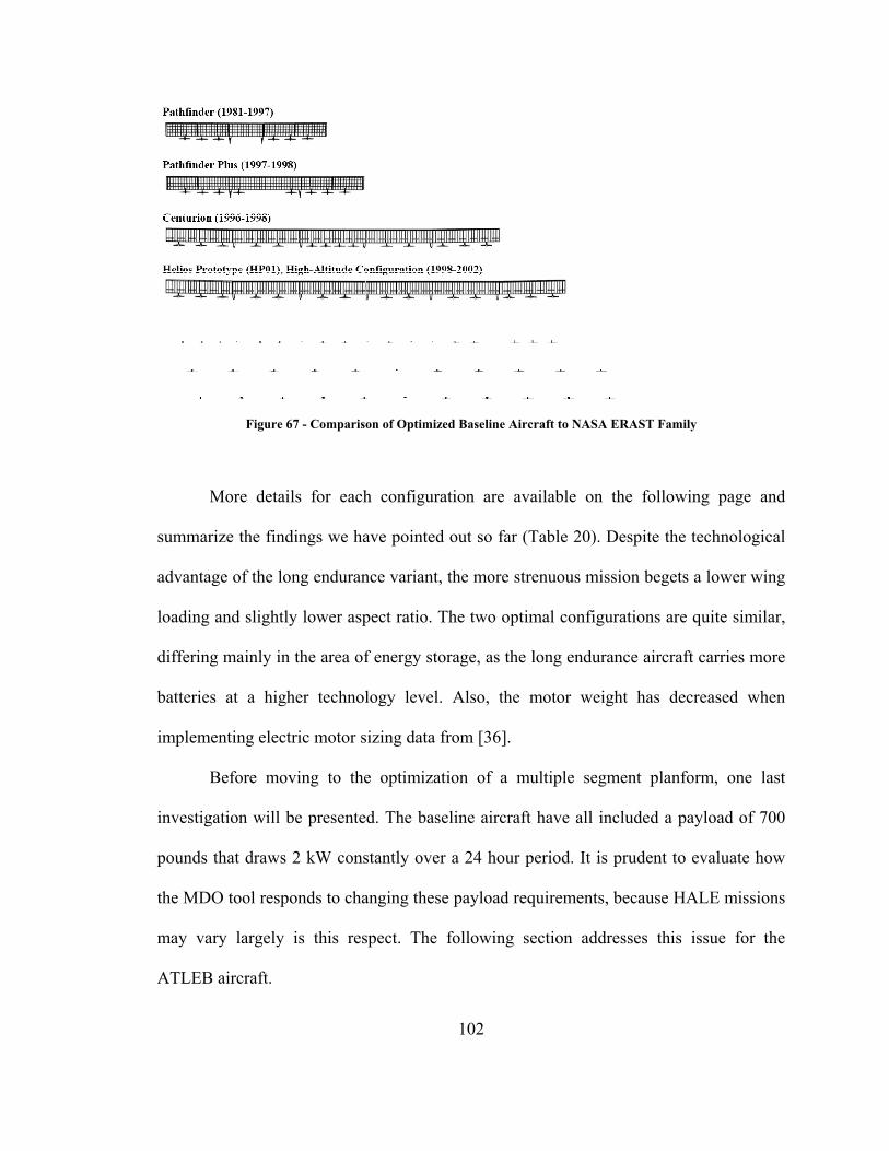
su
ad
lo
d
b
im
in
p
th
m
A
F
More
ummarize th
dvantage of
oading and s
iffering main
atteries at a
mplementing
Befor
nvestigation
ounds that d
he MDO too
may vary lar
ATLEB aircr
Figure 67 - Com
details for
he findings w
the long end
slightly lowe
nly in the ar
a higher tec
g electric mo
e moving t
will be pres
draws 2 kW
ol responds to
rgely is thi
raft.
mparison of Opt
each confi
we have poin
durance vari
er aspect rati
rea of energy
chnology le
otor sizing da
o the optim
sented. The
constantly o
o changing t
s respect. T
102
timized Baselin
iguration are
nted out so f
iant, the mor
io. The two
y storage, as
evel. Also, t
ata from [36
mization of
baseline air
over a 24 ho
these payloa
The followin
ne Aircraft to NA
e available
far (Table 2
re strenuous
optimal con
s the long en
the motor w
6].
a multiple
rcraft have a
our period. I
ad requireme
ng section a
ASA ERAST F
on the foll
0). Despite t
mission beg
nfigurations
ndurance airc
weight has
segment pla
all included a
It is prudent
ents, because
addresses th
amily
lowing page
the technolo
gets a lower
are quite sim
craft carries
decreased w
anform, one
a payload of
t to evaluate
e HALE mis
his issue fo
e and
ogical
wing
milar,
more
when
e last
f 700
e how
ssions
or the

103
Table 20 - Baseline Aircraft Summary
PTMEB ATLEB
Gross Weight lbs 1777 1778
Aspect Ratio 37.62 35.61
Wing Loading lb/ft2 0.83 0.72
Power to Weight Watt/lb 7.28 7.07
Wingspan ft 284.43 295.64
Chord ft 7.56 8.30
Sref ft2 2150.66 2454.59
Wing Thickness 30% 30%
CLmax 1.5 1.5
Max Climb Rate fpm 234.4 227.7
Sea Level Vstall ft/s 21.5 20.2
Cruise Dash ft/s 120.5 126.4
Battery Energy kW-hr 22.5 131.8
Payload Weight lb 700 700
Payload Power kW 2 2
Battery Weight lb 542.8 726.3
Solar Weight lb 214.8 122.7
Wing Weight lb 134.7 132.3
Motor Weight lb 100.0 7.9

104
Different Payloads: Weight and Power Requirement
The initial payload of 700 pounds and 2 kW was chosen to represent the upper
echelon of payload weight that Helios claims to support, with a power requirement
intended to envelope several current or past HALE mission concepts. Payload
requirements for the communications platform design challenge posed by the AIAA were
440 pounds that draw 1.5 kW [8]. The Turin Polytechnic University in Turin, Italy
proposed a design supporting a 220 pound 1.3 kW payload [47]. Also, a study of
alternatives and technology requirements for HALE UAVs proposed two separate
missions, a communications payload of 440 pounds drawing 1.5 kW, and a hurricane
science mission supporting an 880 pound, 2.5 kW payload [49].
Rather than analyzing each of these cases individually, the payload requirement is
perturbed both in weight and power on both sides of the current ATLEB values. Figure
68 shows the total weight breakdown of resulting optimal aircraft carrying different
payload weights. The actual parametric change in aircraft weight is skewed by the
substantial payload contribution, so Figure 69 presents just the dependant components.
Figure 68 - Weight Breakdown for Different Payload Weights
400700
1000605
726
977
100
123
161
104
132
188
0
500
1000
1500
2000
2500
400 lb Payload
ATLEB 700 lb Payload
1,000 lb Payload
Wei
ght (
lb)
MotorsWingSolarBatteryPayload Weight

105
Figure 69 - Battery, Solar, and Wing Weight Sensitivity to Payload
In general we expect to see the aircraft component weights increasing to
accommodate a larger payload. Specifics about the resulting configurations are presented
shortly. The second aspect of electric aircraft payload requirements is the power needed.
We return to the baseline payload of 700 pounds and 2 kW to compare aircraft
configurations with varying payload power (Figure 70).
Figure 70 - Weight Breakdown for Different Payload Power
Changing the power of the payload by 1 kW either way seems to affect almost
exclusively the battery weight. One important note is that if the CONOPS is modified
such that the payload is not in operation during the night, the effect of changing the
power requirement is much less, and will simply require more solar coverage of the wing
to power mission operations and supply regenerative energy.
605726
977
100123
161
104
132
188
0
200
400
600
800
1000
1200
1400
400 lb Payload
ATLEB 700 lb Payload
1,000 lb Payload
Wei
ght (
lb)
MotorsWingSolarBattery
700 700 700
520726
934119
123
161
122
132
161
0
500
1000
1500
2000
1 kW Payload
ATLEB 2 kW Payload
3 kW Payload
Wei
ght (
lb)
MotorsWingSolarBatteryPayload Weight

106
Configuration parameters are summarized in Table 21 below. Several points to
notice are that for a heavy or high power payload, the coverage of wing area by solar
cells has increased to roughly 60%. Also, the planforms for the aircraft are essentially the
same, with aspect ratio, wing span, and chord falling close enough to attribute differences
to loose optimization tolerances. What this means is that if an aircraft is designed with
some margin in the spar to account for the slight changes between Figure 69 and Figure
70, the same platform may be used for different payloads. All that would be necessary
would be refitting more or less batteries and reconfiguring the solar panels.
Table 21 - Payload Study Optima Comparison
ATLEB Payload Low Pow. Light High Pow. Heavy
Gross Weight lbs 1778 1546 1277 2071 2463
Aspect Ratio 35.61 37.04 37.96 37.63 36.84
Wing Loading lb/ft2 0.72 0.64 0.54 0.88 1.01
Power to Weight Watt/lb 7.07 6.68 6.04 7.46 8.03
Wing Thickness % 30.0 29.4 30.0 30.0 30.0
Solar Area % 36.9 44.3 38.1 62.0 60.0
Wingspan ft 295.64 300.0 300.0 297.0 300.0
Chord ft 8.30 8.10 7.90 7.90 8.14
With these baselines defined, we now move into the optimization of a multiple
segment wing configuration. Unlike the process of this chapter, the optimization of a
multi-segment wing will not proceed in stages, but begins by immediately including all of
the design variables discussed thus far.

107
VI. SEGMENTED WING OPTIMIZATION
The MDO tool created for this research was built to allow the user to input the
number of separate pin-connected wing segments, automatically modifying the analytical
processes accordingly. All results presented up to this point have designated one wing
segment, and have performed the MDA on a flying wing span loaded architecture. As we
progress now thorough the investigation of multiple wing segments, the same MDA
environment is used, and built-in contingencies allow the same utilization process as
single segment baseline studies.
Initially, it would seem desirable to simply allow the MDO tool to find the
optimum number of wing segments, just as it would any other design variable. Methods
of Integer Programming do exist to solve optimization problems with discrete variables
[29]. The implementation of Integer Programming in MATLAB is the function bintprog
found in the Optimization Toolbox. Technically, the problem at hand falls under the
category of Mixed Integer Programming, where the set of design variables is composed
of both continuous and discrete entries [29]. Unfortunately, bintprog solves only Binary
Integer Programming problems, and requires the solution to take the form of a binary
integer vector. Since the possible values for number of pinned wing segments represents
a relatively small set, rather than implementing a custom Mixed Integer Programming
optimization routine, we simply evaluate optimal solutions for each pinned wing
configuration. What follows is a discussion of the optimization results for increasing
numbers of pinned wing sections, starting with the span divided in half for a two-segment
platform.
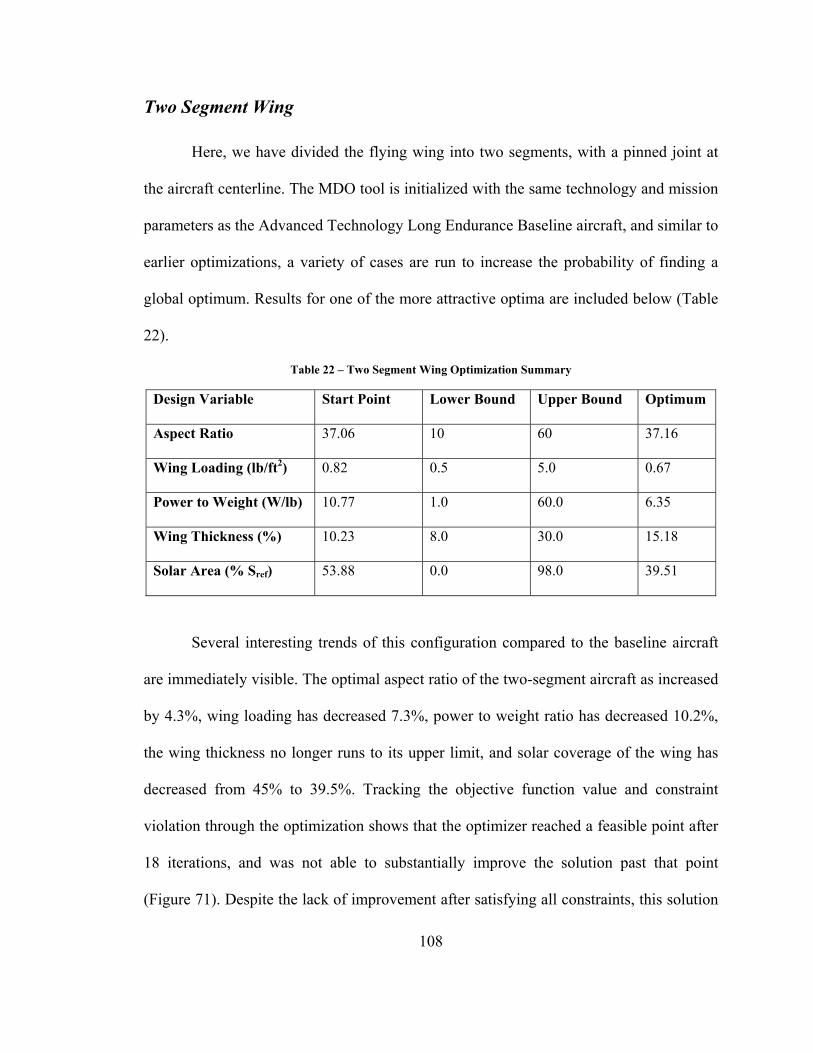
108
Two Segment Wing
Here, we have divided the flying wing into two segments, with a pinned joint at
the aircraft centerline. The MDO tool is initialized with the same technology and mission
parameters as the Advanced Technology Long Endurance Baseline aircraft, and similar to
earlier optimizations, a variety of cases are run to increase the probability of finding a
global optimum. Results for one of the more attractive optima are included below (Table
22).
Table 22 – Two Segment Wing Optimization Summary
Design Variable Start Point Lower Bound Upper Bound Optimum
Aspect Ratio 37.06 10 60 37.16
Wing Loading (lb/ft2) 0.82 0.5 5.0 0.67
Power to Weight (W/lb) 10.77 1.0 60.0 6.35
Wing Thickness (%) 10.23 8.0 30.0 15.18
Solar Area (% Sref) 53.88 0.0 98.0 39.51
Several interesting trends of this configuration compared to the baseline aircraft
are immediately visible. The optimal aspect ratio of the two-segment aircraft as increased
by 4.3%, wing loading has decreased 7.3%, power to weight ratio has decreased 10.2%,
the wing thickness no longer runs to its upper limit, and solar coverage of the wing has
decreased from 45% to 39.5%. Tracking the objective function value and constraint
violation through the optimization shows that the optimizer reached a feasible point after
18 iterations, and was not able to substantially improve the solution past that point
(Figure 71). Despite the lack of improvement after satisfying all constraints, this solution

109
represents the best of 58 separate optimization processes, and gives a gross weight of
1,627 pounds, an 8.5% improvement over the baseline optimum.
Figure 71 – Two Segment Objective Function History
Because the two-segment optimum platform has seen a decrease in wing loading
and an increase in aspect ratio over the baseline, loiter and cruise power requirements
decrease, allowing a reduction in battery energy storage for night flight, corresponding to
a reduced battery weight. Figure 72 compares this optimum with the baseline long
endurance aircraft by weight breakdown, illustrating the 8.3% battery weight reduction.
Another major contributor to the differences between this configuration and the baseline
is the structural weight of the wing, decreasing for the segmented configuration as
expected because we now have essentially two sub-aircraft each with half the aspect ratio
of the overall planform. Decreasing the effective AR for the sub-aircraft provides a 50%
reduction is wing weight. As seen in previous cases, the two-segment aircraft optimum
lies on the wingspan constraint of 300 ft. Compared to the baseline, the aircraft here has
nearly the same reference area, differing only 1.4% because its wingspan is only 295 ft
and it has a larger chord than the two-segment optimum. Now, because of our reduced
0 5 10 15 20 251450
1500
1550
1600
1650
1700
1750
1800
Iterations
Wto

110
battery requirement, the solar area coverage may be decreased. Accordingly, with a
similar wing area but having 5.5% fewer solar cells, a decrease in solar power system
weight is observed.
Figure 72 - Weight Comparison for Two Segment Aircraft
We have pointed out several times that the non-smooth nature of the objective
function response surface encourages multiple optimization runs from different starting
points. From the set of solutions, the best candidate may be chosen, and the result in
Table 22 and Figure 72 is one such selection. When making a selection in this manner, it
is prudent to examine the results and trends to provide some background understanding
of the design space. Figure 73 is a matrix of plots depicting all of the MDO solutions for
each individual design variable compared to every other. The plots show the starting
points as hollow circles, illustrating the Monte Carlo style in which they are randomly
distributed over some domain. Solution points are the filled points, and are colored
according to the resulting gross weight of that specific case. For Figure 73, the lowest
weight points are colored blue and are more or less clustered in some fashion. There are
some outliers and diverging points, but in general, our choice of a global optimum
700 700
726 666
123106
13266
0
200
400
600
800
1000
1200
1400
1600
1800
Long Endurance Baseline
2 Wing Segments
Wei
ght (
lbs) Motors lb
Wing lbSolar lbBattery lbPayload Weight lb

111
(designated by a star outlined in magenta) is surrounded closely by other low weight
points. For a well behaved monotonic objective function with one global minimum, all of
the filled points would fall on top of one another, clearly illustrating the existence of local
minima in our HALE MDO environment. One possible cause of this behavior is the
loosening of convergence tolerances to decrease run time. Loose tolerances coupled with
a response surface that is somewhat flat near the optimum as evidenced by the somewhat
wide clustering of points with similar weight values in Figure 73 will invariably result in
the variety of solutions that we see.
Figure 73 - Plot Matrix of All Optimization Cases for a Two Segment Platform
0.6
0.8
1
1.2
WoS
810121416
PoW
0.1
0.2
0.3
t/c
20 30 40
4050607080
%A so
l
AR0.5 1
WoS8 10 12 14 16
PoW0.1 0.2 0.3
t/c
Starting PointsOptima Colored by WTOSelected Global Optimum
1700
1800
1900
2000
2100

112
Several other methods for visualizing the optimization results and trends highlight
some of the interesting behaviors of the design space. Figure 74 is a scatter plot showing
the gross weight of the solution against wing loading. Points in Figure 74 are colored by
aspect ratio. This plot illustrates a division among the solutions into two regions.
Solutions clustered at the low wing loading value have run into the lower bound imposed
on wing loading, and exhibit a trend of lower aspect ratios than the other solution cluster.
In the area surrounding the selected global optimum, solutions are of lower gross weight,
higher wing loading, and higher aspect ratio. Though a higher aspect ratio in general will
increase the wing weight, our gross weight is dominated by payload weight (a constant
for all points) and battery weight. What we see then, is that the benefits from lower
required power and decreased battery weight from the high aspect ratio wing outweigh
the structural penalty.
Figure 74 – Two Segment MDO Solution Space
0.45 0.5 0.55 0.6 0.65 0.7 0.75 0.8 0.85 0.91600
1700
1800
1900
2000
2100
2200
Wing Loading (lb/ft2)
Gro
ss W
eigh
t (lb
)
Colored by Aspect Ratio
20
25
30
35
40
45

113
Another illustration of this bifurcation of the solutions is presented with the set of
graphs in Figure 75. Here, the solutions are sorted in order of increasing gross weight,
and colored according to various aircraft characteristics, reiterating several clear trends.
First, the solutions that converge to 1800 pounds (the higher weight) all show an aspect
ratio of 25, a wing loading of 0.5, and the lower bound on wing thickness.
Figure 75 – Two Segment Solutions Sorted by Gross Weight
Delving deeper into these solutions, we find that one of the major discriminators
between the low weight plateau and the higher weight group is the battery charge profile.
One reason that two groups of solutions exist is that the optimization environment fails to
1600
1800
2000
2200W
eigh
t (lb
)
Colored byAR
20
30
40
1600
1800
2000
2200
Wei
ght (
lb)
Colored byWoS
0.5
0.60.7
0.8
1600
1800
2000
2200
Wei
ght (
lb)
Colored byPoW
8
10
12
1600
1800
2000
2200
Wei
ght (
lb)
Colored byt/c
0.1
0.2
0.3
1600
1800
2000
2200
Wei
ght (
lb)
Colored by%Asol
0.40.50.60.7
1600
1800
2000
2200
Wei
ght (
lb)
Optimization Run
Colored bySref
2000
3000
4000

114
sufficiently minimize solar coverage in the high weight cases. The resulting charge
profiles resemble Figure 30 with plateaus of stored energy. This, however, does not fully
explain what is happening. If we look at the design variable history for a variety of cases
in the lower cluster compared to those of higher weight, another trend emerges. It appears
that the search direction for the second iteration causes the wing loading variable to run
into its lower bound and remain there for the rest of the optimization. Three examples are
shown below (Figure 76).
Figure 76 - Design Variable History for Anomalous Solutions
This behavior is in contrast to that seen with the lower weight solutions, shown in Figure
79. Here we see that the wing loading value (teal) may hit the lower bound, but does not
remain at the same value throughout the optimization. Table 23 summarizes the solution
clusters, providing the average for each group.
Wto e3Wwing e2AR e1WoS e0PoW e1t/c e-1Percent Solar
0 5 10 15 200
0.5
1
1.5
2
2.5
3
3.5
4
4.5
Iteration Number
0 2 4 6 8
0
0.5
1
1.5
2
2.5
3
3.5
4
4.5
5
Iteration Number
0 5 10 15 20
0
0.5
1
1.5
2
2.5
3
3.5
4
4.5
5
Iteration Number
g p

115
Figure 77 - Design Variable History for Attractive Solutions
Table 23 - Average Values for Solution Clusters
Low Weight Group High Weight Group Mean Std. Dev. Mean Std. Dev.
Aspect Ratio 38.3 3.92 25.3 1.05
Wing Loading (lb/ft2) 0.72 0.07 0.51 0.03
Power to Weight (W/lb) 6.9 0.87 7.4 1.36
Wing Thickness (%) 20.2 8.14 11.4 6.19
Solar Area (% Sref) 45.4 6.54 37.5 5.63
The root cause of the difference between the two solution clusters, however, has
been traced to the aerodynamics module, and the use of EDET as a drag code. Currently,
the implementation of EDET does not model a continuously changing laminar to
turbulent transition point on the wing. Rather, the code flags either a fully turbulent or a
fully laminar boundary layer based on whether the Reynolds’ Number based on chord is
below or above 500,000. This sort of discrete change in a variable or quantity, especially
one as central as the drag coefficient, will definitely cause problems for our optimizer,
and in this case, results in a divided solution space. Figure 78 shows that the cluster of
0 5 10 15 200
1
2
3
4
5
6
Iteration Number
g p
0 5 10 15 200
0.5
1
1.5
2
2.5
3
3.5
4
4.5
5
Iteration Number
0 5 10 15 20 25
0
1
2
3
4
5
6
Iteration Number

116
low weight solutions, because of their higher wing loading and aspect ratio, are below the
cutoff for turbulent boundary layer friction coefficient equations, and are assumed to be
laminar.
Figure 78 - Two Segment Solutions: Reynolds' Number
Because the goal for these MDO processes was minimization of gross weight, we
focus on the low weight cluster when choosing the optimal two segment configuration.
Indeed, all of the points in Figure 73, Figure 74, and Figure 75 are optima in the sense
that they have met the constraints imposed and the optimizer has found the minimum
weight for some tolerance. We therefore have selected the point shown as a star in the
figures and described in Table 22 to represent the best design of this architecture. Mean
values from Table 23 are presented only for illustrative purposes.
0.4 0.5 0.6 0.7 0.8 0.91600
1700
1800
1900
2000
2100
2200
Wing Loading (lb/ft2)
Gro
ss W
eigh
t (lb
)
Colored by Cruise Reynolds' Number
4
4.5
5
5.5
6
6.5
7
x 105

117
Additional Wing Segments
The same procedures described for the two segment wing are used to evaluate any
number of pinned wing segments. Rather than presenting specific results one at a time for
each case, results are discussed here comparing the set of two to six wing segments.
Optimum configurations for the various pinned wing platforms are all selected as the
minimum weight solution from a large set of optimization runs. The weight breakdowns
for the best solutions are compared in Figure 79.
Figure 79 - Weight Breakdown Comparison of Multiple Wing Segment Configurations
The most noticeable aspect of this chart is that with an increasing number of wing
segments, the weight of the optimal aircraft converges to similar values and benefits of
additional segments disappear. Of all the parameters and characteristics of each optimal
aircraft configuration, one of the more interesting ones to explore when looking at
increasing the number of wing segments is the wing thickness. We expected that
700 700 700 700 700 700
726 666 638 619 622 611
123 106 102 99 99 110
13266
0
200
400
600
800
1000
1200
1400
1600
1800
Wei
ght (
lbs)
Motors lbWing lbSolar lbBattery lbPayload Weight lb

118
increasing the number of segments would decrease the structural loading on the spar, and
Figure 79 confirms this. What happens with the higher number of segments is that the
wall thickness of the spar that is required to support the loads decreases to the minimum
allowable value of 0.005 inches. Earlier, it was shown that the aerodynamic analysis
process is sensitive to wing thickness (Figure 27) and higher thickness results in a higher
CDo. Since wing thickness is a design variable, and spar wall thickness is constrained by a
lower bound, the optimizer decreases the wing thickness to chord ratio to reduce power
required, battery weight, solar weight, etc. A thinner wing results in a smaller spar cross
section and increased principal stresses, so we imagine that there exists a Pareto front of
low spar weight and low wing thickness. One segment designs showed a tendency toward
high thickness because the aerodynamic benefits of a thin wing were outweighed by the
large increases in structural weight. Figure 80 tracks the wing thickness for different
numbers of wing segments, and we see the upper bound of 30% thickness to chord ratio
for a single segment wing. Also apparent is the ability of the optimizer, when analyzing a
multiple segment configuration, to decrease the thickness some amount before seeing the
structural penalty. Compared to the single segment, t/c is halved for two segments.
Figure 80 - Optimal Wing Thickness for Multiple Wing Segments
00.05
0.10.15
0.20.25
0.30.35
1 2 3 4 5 6
Win
g T
hick
ness
(t/c
)
Number of Pinned Wing Segments

119
Next, we look back to Table 22 and have represented the upper and lower bounds
for the thickness to chord design variable as red lines on Figure 80. It seems that for more
wing segments, the lower structural loads facilitate thinner and thinner wings, eventually
encountering the lower bound on the variable. Keep in mind that Figure 80 actually
represents the wing thickness as a percent of chord length, and that we haven’t quoted
any actual maximum thickness values. This means that the optimizer may have arrived at
a minimum thickness to chord ratio, but can still further decrease the actual thickness
value by decreasing the chord. Figure 81 shows that if the aircraft has more than 4 wing
segments, there is a sharp decline in chord length, and with the wingspan at the upper
limit of 300 ft for all cases, this translates directly to a sharp decrease in Sref (Figure 82).
Figure 81 - Optimal Wing Chord for Multiple Wing Segments
Figure 82 - Optimal Sref for Multiple Wing Segments
6.5
7
7.5
8
8.5
1 2 3 4 5 6
Win
g C
hord
(ft)
Number of Pinned Wing Segments
2000
2100
2200
2300
2400
2500
1 2 3 4 5 6
Ref
eren
ce A
rea
(ft2
)
Number of Pinned Wing Segments

120
Another result of the change lower bound on thickness to chord ratio becoming
active is apparent in the percent of the wing requiring coverage. The actual area of solar
cells for each case is generally similar, so decreasing the wing area simply means that a
greater percent of the wing must be covered (Figure 83).
Figure 83 - Optimal Solar Coverage (Percent)
While Figure 79 shows slight improvements in structural weight between 3, 4,
and 5 segments, the reality is that the gross weight of the aircraft is nearly the same
(Figure 84). When reference area is decreased for an aircraft with a given weight, the
result is a higher wing loading, a result that we see in Figure 85.
Figure 84 - Optimal Gross Weight for Multiple Wing Segments
0
0.1
0.2
0.3
0.4
0.5
1 2 3 4 5 6
Sola
r C
ell A
rea
(%)
Number of Pinned Wing Segments
1500155016001650170017501800
1 2 3 4 5 6
Gro
ss W
eigh
t (lb
s)
Number of Pinned Wing Segments

121
Figure 85 - Optimal Wing Loading for Multiple Wing Segments
We might expect that higher wing loading would increase required power, battery
weights, etc, but the results in Figure 79 and Figure 84 do not show this happening. In
fact, the optimizer has increased the aspect ratio, made possible within the wingspan
constraint because of the decreased chord length for higher numbers of wing segments.
Figure 86 tracks aspect ratio for each configuration.
Figure 86 - Optimal Aspect Ratio for Multiple Wing Segments
0.64
0.66
0.68
0.7
0.72
0.74
1 2 3 4 5 6
Win
g L
oadi
ng (l
b/ft
2 )
Number of Pinned Wing Segments
30
35
40
45
50
1 2 3 4 5 6
Asp
ect R
atio
Number of Pinned Wing Segments

122
CONCLUSION
The central goal of this research was the development of a multidisciplinary tool
for analysis, design, and optimization of HALE UAVs, facilitating the study of a novel
configuration concept. Applying design ideas stemming from a unique WWII-era project,
a “pinned wing” HALE aircraft would employ self-supporting wing segments assembled
into one overall flying wing. The research effort began with the creation of a
multidisciplinary analysis environment comprised of analysis modules, each providing
information about a specific discipline. As the modules were created, attempts were made
to validate and calibrate the processes against known data, culminating in a validation
study of the fully integrated MDA environment. Using the NASA / AeroVironment
Helios aircraft as a basis for comparison, with generalized Helios payload and mission
data, the included MDA environment sized a vehicle to within 5% of the actual
maximum gross weight. Because certain mission specifics for Helios were unclear or
non-specific, like battery weight or cruise profile, several sensitivity studies were
completed. In addition to showing correct trends and system responses to certain variable
perturbations, these studies identified some of the stronger drivers of aircraft weight, like
energy storage technology or mission definition (cruise altitude and endurance). With
reassurance that the tool provides reasonable results and correct trends, the whole process
was wrapped in an optimization environment for further study.
Because of the parametric approach to the problem at hand, comparison of
optimum results is focused on evaluating the change from some baseline configuration.
First, the Helios-based validation case was re-posed as an optimization problem to see if

123
any improvements were possible. Here, improvements may be in the form of reduced
gross weight, or enhanced mission capabilities. For Helios technology and a medium-
endurance mission (14-15 hours) the MDO tool shows a 17.3% reduction in gross weight,
largely due to a thicker wing for structural weight reduction, and an optimized planform
for low power flight, reducing battery weight. Next, more advanced technology
parameters were used with the Helios-style aircraft to perform a long-endurance mission
with requirements similar to the DARPA Vulture program. With 10% more efficient solar
cells, a 92% net power train efficiency, and advanced batteries, the aircraft was able to
achieve day/night operation at a gross weight nearly identical to the optimized medium-
endurance configuration. All subsequent optimizations consider advanced technology
components and a long endurance mission, so this last case is used as a baseline for
comparison of the segmented wing concept.
When applying the MDO tool to a multi-segment flying wing architecture, we
expect that the reduced aspect ratio of each individual wing section should reduce the
overall structural weight of the aircraft. Indeed, moving from the baseline to a two
segment wing allows a 50% reduction in wing structural weight in addition to lowered
battery and solar weights. Overall, the two segment wing provides an 8.5% reduction in
gross weight over the long-endurance baseline for the same mission and payload
requirements. It was shown that increasing the number of wing segments provides
diminishing benefit, and that when certain constraints are activated, like the lower bound
of t/c, some solution trends may change but the resulting gross weight is not greatly
affected. For the six segment configuration, the MDO tool predicts a 14.2% decrease in
weight compared to the long endurance baseline.

124
Upon conception of this research effort, it was thought that implementing a
pinned wing concept may facilitate aircraft of extremely high aspect ratio and great
improvement over a one-piece wing. We have shown that in fact the concept does allow
for reduced structural weight, low wing loading, and optimal aspect ratios in the high 30s
to low 40s. However, with advancements in energy storage technologies, highly efficient
propulsion devices, and a careful spanwise mass distribution applied to a one-piece flying
wing, many of the same benefits are possible. The added complexity inherent in a pinned
wing configuration, and the associated risk detract from the potential benefits. Where we
initially expected drastic improvements, results from the MDO tool suggest that actual
benefits may not be quite as outstanding.
125
FUTURE WORK
Due to the modular nature of the MDO tool created for this research, one main
area for future work is the improvement of the disciplinary analysis codes. Admittedly,
the author is not an expert in all areas of flight science, composite structural analysis,
aeronautical alternative energy, etc., but the included subroutines are meant to give a
good first order approximation of trends and sensitivities. It may be worthwhile to
investigate whether replacing the analysis modules with high-fidelity counterparts
provides different predictions of parametric changes, or deltas.
Some other possible areas for future work may address some of the supplemental
aspects of design that were either not directly addressed in the included study, or were
attempted but not completed. First of note is a modeling of the vehicle in a dynamic
environment capable of performing gust load analysis or structural dynamic responses.
ASWING is a program developed to evaluate structural, aerodynamic, and control
response characteristics of aircraft with high aspect ratio wings and highly flexible
structures [56]. Currently the MDO tool creates an ASWING configuration input file that
includes the aerodynamic layout, structural details, and weight distribution. For a single
segment wing, analysis in ASWING is straightforward, but problems were encountered
when defining a multi segment platform. We were unable to develop a sufficient and
accurate set of kinematic constraints for a pinned wing that satisfied ASWING’s
requirements.
Also, the tool applies to a wide range of scales of aircraft, so studies of small
payload aircraft are possible. Or, if keeping with a large payload, alternate CONOPS may

126
lead to modification of optimizer constraints like wingspan and may result in different
vehicle solutions. Other configurations may also be investigated, as small changes in the
tool allow for aircraft that may include conventional tails and tail booms.
Lastly, the basis of the study discussed in this paper was an aircraft that included
chemical batteries as the energy storage medium. However, because the tool implements
the energy system sizing methods presented by Dudley and Misra [36], this may be
changed to completely alter the aircraft concept. Inclusion of a fuel-cell based power
system is simply a matter of changing one input flag, and new propulsive efficiencies are
calculated, new components are sized for the weight statement including things like
hydrogen tanks, and new energy density values are used.

127
REFERENCES
[1] Hall, D. W., Watson, D. A., Tuttle, R. P., and Hall, S. A., “Mission Analysis of Solar Powered Aircraft,” NASA CR-172583, July 1985.
[2] Phillips, W. H., “Some Design Considerations for Solar-Powered Aircraft,” NASA-TP-1675. June, 1980.
[3] Hall, D. W., Fortenbach, C. D., Dimiceli, E. V., and Parks, R. W., “A Preliminary Study of Solar Powered Aircraft and Associated Power Trains,” NASA-CR-3699. Dec, 1983.
[4] Romeo, G., Frulla, G., Cestino, E., and Corsino, G., “HELIPLAT: Design, Aerodynamic, Structural Analysis of Long-Endurance Solar-Powered Stratospheric Platform,” AIAA Journal of Aircraft, 2004. Vol. 41, no. 6 (1505-1520).
[5] “Vulture Program: Broad Agency Announcement (BAA) Solicitation 07-15,” Defense Advanced Research Projects Agency, DARPA/TTO. Arlington, VA. July, 2007.
[6] Carty, A., “An Approach to Multidisciplinary Design, Analysis and Optimization For Rapid Conceptual Design,” 9th AIAA/ISSMO Symposium on Multidisciplinary Analysis and Optimization.. Sept. 2002. AIAA 2002-5438.
[7] Logan, T. R., “Strategy for Multilevel Optimization of Aircraft,” AIAA Journal of Aircraft, 1990. Vol. 27, no. 12 (1068-1072).
[8] “2007-2008 AIAA Graduate Team Aircraft Design Competition,” AIAA Student Programs, Reston, VA.
[9] Noth, A., “History of Solar Flight,” Anonymous Systems Lab, ETH, Zurich, Switzerland., Jul. 2008.
[10] “History of Electric Flight,” URL: http://www.iriquois.free-online.co.uk/hist.htm . [cited 28 Apr 2009].
[11] “Overview of Energy Storage Methods,” MORA Associates, URL: http://www.moraassociates.com . [cited 28 Apr 2009].
[12] “Lithium Sulfur Rechargeable Battery Data Sheet,” SION Powe Inc., URL: http://www.sionpower.com/pdf/sion_product_spec.pdf . [cited 28 Apr 2009].
[13] Tudron, F. B., Akridge, J. R., and Puglisi, V. J., “Lithium-Sulfur Rechargeable Batteries: Characteristics, State of Development, and Applicability to Powering Portable Electronics,” Scion Power Corporation, Tucson AZ, 2004.
[14] Dents, D. J., “Solar Airplanes and Regenerative Fuel Cells,” Electrochemistry Branch, NASA Glenn Research Center at Lewis Field, 9 Oct. 2007.
[15] “The History of Solar,” U.S. Department of Energy, Energy Efficiency and Renewable Energy, URL: http://www1.eere.energy.gov/solar/pdfs/solar_timeline.pdf . [cited 29 Apr 2009].
[16] “AC Propulsion’s Solar Electric Powered Solong UAV,” AC Propulsion, 2 Dec. 2004.
[17] “Solar-Power Research at Dryden,” NASA Facts, Dryden Flight Research Center FS-1998-10-0054 DFRC.
[18] “Pathfinder and the Development of Solar Rechargeable Aircraft,” URL: http://www.llnl.gov/etr/pdfs/07_94.1.pdf . [cited 28 Apr 2009].
[19] “NASA Dryden Fact Sheet – Pathfinder Solar-Powered Aircraft,” URL: http://www.nasa.gov/centers/dryden/news/FactSheets/FS-034-DFRC.html . [cited 28 Apr 2009].
[20] Noll, T. E., Brown, J. M., Perez-Davis, M. E., Ishmael, S. D., Tiffany, G. C., and Gaier, M., “Investigation of the Helios Prototype Aircraft Mishap,” Helios Prototype Aircraft Mishap Investigation Board, 16 Jan 2004.

128
[21] “Helios Prototype: The forerunner of 21st century solar-powered ‘atmospheric satellites’,” NASA Dryden
Flight Research Center, URL: http://www.nasa.gov/centers/dryden/news/FactSheets/FS-068-DFRC.html [cited 1 Feb 2009].
[22] Anderson, C. E., “Dangerous Experiments: Wingtip Coupling at 15,000 Feet,” Flight Journal, Vol. 5, No. 6, p. 64, Dec 2000.
[23] “Convair GRB-36F Peacemaker,” National Museum of the US Air Force, URL: http://www.nationalmuseum.af.mil/factsheets/factsheet.asp?id=2550 . [cited 31 May, 2009].
[24] Miller, J., “Project ‘Tom-Tom’,” Aerophile, Vol. 1, No. 3, pp. 161-164, Dec 1977.
[25] Diedrich, F. W., and Zlotnick, M., “Calculated Lift Distributions of a Consolidated Vultee B-36 and Two Boeing B-47 Airplanes Coupled at the Wing Tips,” National Advisory Committee for Aeronautics. NACA RM L50I26. Nov 30, 1950.
[26] Jensen, S.C., Rettie, I.H., and Barber, E.A., “Role of Figures of Merit in Design Optimization and Technology Assessment,” Journal of Aircraft, Vol. 18, No. 2, Feb 1981.
[27] “Cost and Business Model Analysis for Civilian UAV Missions,” Moiré Incorporated, June 8, 2004.
[28] “Constrained Optimization,” The MathWorks, Inc., Optimization ToolboxTM, MATLAB Documentation, 1984-2008.
[29] Fletcher, R., Practical Methods of Optimization, Second Edition, John Wiley & Sons Ltd, West Sussex, England, 1987.
[30] Kroo, I, “Distributed Multidisciplinary Design and Collaborative Optimization,” VKI lecture series on Optimization Methods & Tools for Multicriteria/Multidisciplinary Design, Stanford University, Nov. 2004.
[31] Sobiesxcxanski-Sobieski, J., “A Linear Decomposition Method for Large Optimization Problems—Blueprint for Development,” NASA TM-83248, Feb.1982.
[32] Steward, D., “The Design Structure System: A Method for Managing the Design of Complex Systems,” IEE Transactions of Engineering Management, Vol. EM 78. No. 3, Aug. 1981.
[33] Hall, D. W., and Hall, S. A., “Structural Sizing of a Solar Powered Aircraft,” NASA CR-172313, April, 1984.
[34] Frulla, G., and Cestino, E., “Design, manufacturing, and testing of a HALE-UAV structural demonstrator,” Composite Structures, April 2008. Vol. 83, issue 2, pp 143-153. ISSN 0263-8223.
[35] Nam, T., “A Generalized Sizing Method for Revolutionary Concepts Under Probabilistic Design Constraints,” Ph.D. Thesis, School of Aerospace Engineering, Georgia Institute of Technology, May 2007.
[36] Dudley, M., and Misra, A., “Electric Airplane Power-system Performance Requirements,” The 2009 CAFE Foundation Electric Aircraft Symposium. NASA Ames and Glen Research Centers. 24 Apr. 2009.
[37] Youngblood, J. W., Talay, T. A., and Pegg, R. J., “Design of Long-Endurance Unmanned Airplanes Incorporating Solar and Fuel Cell Propulsions,” AIAA Paper 84-1430, June 1984.
[38] Drela, M., and Youngren, H., “AVL: Aerodynamic Analysis, Trim Calculation, Dynamic Stability Analysis, Aircraft Configuration Development,” Massachusetts Institute of Technology, URL: http://web.mit.edu/drela/Public/web/avl/ . [cited 20 May, 2009].
[39] “Empirical Drag Estimation Technique (EDET) Program Users Manual,” Lockheed California Company, Burbank, CA. LR 28788. 22, Dec 1978.
129
[40] Feagin, R. A. and Morrison, W. D., Jr., “Delta Method, and Empirical Drag Buildup Technique,” NASA CR 151971, Dec 1978.
[41] “Steve Fossett: Always ‘Scouting for New Adventures’ Part 2,” Airport Journals, URL: http://www.airportjournals.com/Display.cfm?varID=0611030 , Nov 2006. [cited 25 May, 2009].
[42] “Non-Stop Solo Around the World,” American Aviation Historical Society, URL: http://www.aahs-online.org/articles/globalflyer.htm . [cited 25 May, 2009].
[43] Duffie, J. A., and Beckman, W. A., Solar Engineering of Thermal Processes, Wiley-Interscience, New York, third edition, 2006.
[44] Noth, A., “Design of Solar Powered Airplanes for Continuous Flight,” Dissertation, Doctor of Technical Sciences, ETH Zurich. Diss. ETH No. 18010. Sept, 2008.
[45] “Solar Impulse Version 1.1 Electrical Values Presentation,” Ecole Polytechnique Federale De Lausanne, Apr. 2004.
[46] Raffaelle, R. R., Harris, J. D., Hehemann, D., Scheiman, D., Rybicki, G., and Hepp, A. F., “Integrated Thin-Film Solar Power System,” Energy Conversion Engineering Conference and Exhibit, 2000. (IECEC) 35th Intersociety, vol.1, no., pp.58-62 vol.1, 2000.
[47] Cestino, E., “Design of Solar High Altitude Long Endurance Aircraft for Multi Payload & Operations,” Department of Aerospace Engineering, Politecnico di Torino, Turin, Italy. June 2006.
[48] Colozza, A. J., “Effect of Power System Technology and Mission Requirements on High Altitude Long Endurance Aircraft,” NASA CR-194455. Nov. 1993.
[49] Nickol, C. N., Guynn, M. D., Kohout, L. L., and Ozoroski, T. A., “High Altitude Long Endurance UAV Analysis of Alternatives and Technology Requirements Development,” NASA/TP-2007-214861. Mar. 2007.
[50] “Our Tax Dollars at Work,” URL: http://www.stango.net/helios.htm .[cited 25 May, 2009].
[51] Center for Composite Material Research, North Carolina A&T State University, http://www.ncat.edu/~ccmradm/ccmr/ [cited 20 Apr. 2009].
[52] Quantum Composites Lytex® 4149 55% Carbon Fiber Epoxy SMC Data Sheet. MatWeb Material Property Data. http://www.matweb.com/search/DataSheet.aspx?MatGUID=3b8b3df085d2448fad7436fa7c492107 [cited 1 May 2009].
[53] Wainfan, B., “Aerodynamics of Long Endurance Flight,” ACA Industries, Inc., Cal Poly Aircraft Design Lab Library XA 500.
[54] Baraaclough, J., “Electric Propulsion Platforms at DFRC,” NASA DFRC-943. 10, Apr. 2009.
[55] Chan, C. K., Peng, H., Liu, G., McIlwrath, K., Zhang, X. F., Huggins, R A., Cui, Y., “High-performance Lithium Battery Anodes Using Silicon Nanowires,” Nature Nanotechnology. 16 Dec. 2007.
[56] Drela, M., “ASWING Configuration Development System for Flexible Aircraft,” Massachusetts Institute of Technology, URL: http://web.mit.edu/drela/Public/web/aswing/ . [cited 29 May, 2009].