Multidimensional Summation-By-Parts Operators:General Theory and Application to Simplex ElementsI

Jason E. Hickena,1,∗, David C. Del Rey Fernandezb,2, David W. Zinggb,3

aDepartment of Mechanical, Aerospace, and Nuclear Engineering,Rensselaer Polytechnic Institute,Troy, New York, United StatesbInstitute for Aerospace Studies,

University of Toronto,Toronto, Ontario, M3H 5T6, Canada

Abstract

Summation-by-parts (SBP) operators offer the efficiency of finite-difference methods with the prov-able time stability of Galerkin finite-element methods, but they have traditionally been limited totensor-product domains. This paper presents a definition for multidimensional SBP finite-differenceoperators that is a natural extension of the classical one-dimensional SBP definition. Theoreticalimplications of the definition are investigated for the special case of a diagonal-norm (mass) matrix,and it is shown that the operators retain the desirable properties of tensor-product SBP opera-tors. A cubature rule with positive weights is proven to be a necessary and sufficient conditionfor the existence of diagonal-norm SBP operators on a particular domain. Concrete examples ofmultidimensional SBP operators are constructed for the triangle and tetrahedron; similarities anddifferences with spectral-element and spectral-difference methods are discussed. An assembly pro-cess is described that builds diagonal-norm SBP operators on a global domain from element-leveloperators. Numerical results of linear advection on a doubly periodic domain demonstrate theaccuracy and time stability of the simplex operators.

Keywords: summation-by-parts, finite-difference method, unstructured grid, spectral-elementmethod, spectral-difference method, mimetic discretization

1. Introduction

Summation-by-parts (SBP) operators are high-order finite-difference schemes that mimic thesymmetry properties of the differential operators they approximate [1]. Respecting such symmetrieshas important implications; in particular, they enable SBP discretizations that are both time-stable

IThis work was supported by Rensselaer Polytechnic Institute and the Natural Sciences and Engineering ResearchCouncil (NSERC) of Canada∗corresponding authorEmail addresses: hickej2@rpi.edu (Jason E. Hicken), dcdelrey@oddjob.utias.utoronto.ca

(David C. Del Rey Fernandez), dwz@oddjob.utias.utoronto.ca (David W. Zingg)1Assistant Professor2Graduate Student3Professor and Director

Preprint submitted to Elsevier May 12, 2015

and high-order accurate [2–4], properties that are essential for robust, long-time simulations ofturbulent flows [5, 6].

Most existing SBP operators are one-dimensional [7–10] and are applied to multidimensionalproblems using a multi-block tensor-product formulation [11–13]. Like other tensor-product meth-ods, the restriction to multi-block grids complicates mesh generation and adaptation, and it limitsthe geometric complexity that can be considered in practice.

The limitations of the tensor-product formulation motivate our interest in generalizing SBPoperators to unstructured grids. There are two ways this generalization has been pursued in theliterature: 1) construct global SBP operators on an arbitrary distribution of nodes, or; 2) constructSBP operators on reference elements and assemble a global discretization by coupling these smallerelements.

While the first approach is appealing conceptually, it presents challenges. Kitson et al. [14]showed that, for a given stencil width and design accuracy, there exists grids for which no stable,diagonal-norm SBP operator exists. Thus, building stable high-order SBP operators on arbitrarynode distributions may require unacceptably large stencils. When SBP operators do exist for agiven node distribution, they must be determined globally by solving a system of equations, ingeneral. The global nature of these SBP operators is exemplified in the mesh-free framework ofChiu et al. [15, 16].

The second approach — constructing SBP operators on reference elements and using theseto build the global discretization — is more common and presents fewer difficulties. The primarychallenge here is to extend the one-dimensional SBP operators of Kreiss and Scherer [1] to a broaderset of operators and domains. The existence of such operators, at least in the dense-norm case4,was established by Carpenter and Gottlieb [17]. They proved that operators with the SBP propertycan be constructed from the Lagrangian interpolant on nearly arbitrary nodal distributions, whichis practically feasible on reference elements with relatively few nodes. More recently, Gassner[18] showed that the discontinuous spectral-element method is equivalent to a diagonal-norm SBPdiscretization when the Legendre-Gauss-Lobatto nodes are used with a lumped mass matrix.

Of particular relevance to the present work is the extension of the SBP concept by Del ReyFernandez et al. [19]. They introduced a generalized summation-by-parts (GSBP) definition for ar-bitrary node distributions on one-dimensional elements, and these ideas helped shape the definitionof SBP operators presented herein.

Our first objective in the present work is to develop a suitable definition for multi-dimensionalSBP operators on arbitrary grids and to characterize the resulting operators theoretically. We notethat the discrete-derivative operator presented in [15] is a possible candidate for defining (diagonal-norm) multi-dimensional SBP operators; however, it lacks properties of conventional SBP operatorsthat we would like to retain, such as the accuracy of the discrete divergence theorem [20].

Our second objective is to provide a concrete example of multi-dimensional diagonal-norm SBPoperators on non-tensor-product domains. We follow the element-based approach and constructSBP operators for triangular and tetrahedral elements. The resulting operators are similar to thoseused in the nodal triangular-spectral-element method [21–23]. Unlike the spectral-element methodbased on cubature points, we do not insist on a polynomial basis and use the resulting freedom toenforce the summation-by-parts property; this leads to provably time-stable schemes.

The remaining paper is structured as follows. Section 2 presents notation and the proposeddefinition for multi-dimensional SBP operators. We study the theoretical implications of the pro-

4In this paper, norm matrix is synonymous with mass matrix.

2

posed definition in Section 3. We then describe, in Section 4, how to construct diagonal-normSBP operators for the triangle and tetrahedron. Section 4 also establishes that SBP operators onsubdomains can be assembled into SBP operators on the global domain. Results of applying thetriangular SBP operators to the linear advection equation are presented in Section 5. Conclusionsare given in Section 6.

2. Preliminaries

To make the presentation concise, we concentrate on multi-dimensional SBP operators in twodimensions; the extension to higher dimensions follows in a straightforward manner. Furthermore,in many cases we present definitions and theorems for operators in the x coordinate direction only.

2.1. Notation

We consider discretized derivative operators defined on a set of n nodes, S = (xi, yi)ni=1.Capital letters with script type are used to denote continuous functions. For example, U(x) ∈ L2(Ω)denotes a square-integrable function on the domain Ω. We use lower-case bold font to denote therestriction of functions to the nodes. Thus, the restriction of U to S is given by

u = [U(x1, y1), . . . ,U(xn, yn)]T . (1)

Following this convention, the nodes themselves will often be represented by the two vectors x =[x1, . . . , xn]T and y = [y1, . . . , yn]T. More generally, the restriction of monomials to S is represented

by xj =[xj1, . . . , x

jn

]Tand yj =

[yj1, . . . , y

jn

]T, with the convention that xj = yj = 0 if j < 0. We

use the element-wise Hadamard product, denoted , to represent the product of functions restrictedto the nodes. For example, the restriction of xayb to S is given by xa yb.

Matrices are represented using capital letters with sans-serif font; for example, the first deriva-tive operators with respect to x and y are represented by the matrices Dx and Dy, respectively.Entries of a matrix are indicated with subscripts, and we follow Matlab R©-like notation when ref-erencing submatrices. For example, A:,j denotes the jth column of matrix A, and A:,1:k denotes itsfirst k columns.

2.2. Multidimensional SBP operator definition

We propose the following definition for Dx, the SBP first-derivative operator with respect tox. An analogous definition holds for Dy and, in three-dimensions, Dz. Definition 1 is a naturalextension of the definition of GSBP operators proposed in [19], which itself extends the classicalSBP operators introduced by Kreiss and Scherer [1].

Definition 1. Two-dimensional summation-by-parts operators: Consider an open andbounded domain Ω ⊂ R2 with a piecewise-smooth boundary Γ. The matrix Dx is a degree p SBPapproximation to the first derivative ∂

∂x on the nodes S = (xi, yi)ni=1 if

i) Dxxax yay = axx

ax−1 yay , ∀ ax + ay ≤ p;

ii) Dx = H−1Sx = H−1(Qx + 1

2Ex

), where Qx is antisymmetric, and Ex is symmetric;

iii) H is symmetric positive definite, and;

iv) (xax yay)T Exxbx yby =

∮Γxax+bxyay+bynxdΓ, ∀ ax + ay, bx + by ≤ τEx,

where τEx ≥ p and n = [nx, ny]T is the outward pointing unit normal to the surface Γ.

3

Before studying the implications of Definition 1 in Section 3, it is worthwhile to motivate andelaborate on each of the four properties in the definition.

Property i ensures that Dx is an accurate approximation to the first-partial derivative withrespect to x. It does this in the usual way by requiring that the operator be exact for polynomialsof total degree less than or equal to p. Consequently, in two dimensions the minimum number ofnodes necessary to satisfy property i is

nmin =(p+ 1) (p+ 2)

2. (2)

For d dimensions it is necessary to have at least(p+dd

)nodes. Unlike finite-element methods, SBP

operators generally need more nodes than required by the accuracy conditions, in order to satisfyproperties ii–iv.

Property ii is needed for the SBP operator to mimic integration by parts (IBP). Recall thatthe IBP formula for the x derivative is∫

ΩV ∂U∂x

dΩ =

∮ΓVUnxdΓ−

∫ΩU ∂V∂x

dΩ,

where the outward-pointing unit normal to the surface is n = [nx, ny]T. The SBP approximationof IBP follows immediately from property ii:

vTHDxu = vTExu− uTHDxv, ∀ v,u ∈ Rn. (3)

The matrix H must be symmetric positive-definite to guarantee stability: without property iii,the discrete “energy”, uTHu, could be negative when uTu > 0, and vice versa. The so-called normmatrix H can be interpreted as a mass matrix, i.e.

Hi,j =

∫Ωφi(x)φj(x)dΩ,

but it is important to emphasize that SBP operators are finite-difference operators, and there isno (known) closed-form expression for the basis φini=1, in general. In the diagonal norm case, weshall show that another interpretation of H is as a cubature rule.

Finally, property iv implies that Ex is a degree τEx approximation to the surface integral∮ΓVUnxdΓ. (4)

While property iv is not explicitly present in one-dimensional SBP definitions [1, 7], it is implicitlysatisfied by tensor-product SBP operators [20]. For general domains, property iv must be explicitlyenforced in order to approximate the surface integral in IBP accurately, and, consequently, retaindesirable properties like dual consistency [24].

3. Analysis of diagonal-norm multi-dimensional summation-by-parts operators

In this section, we determine the implications of Definition 1 on the constituent matrices of amulti-dimensional SBP operator and whether or not such operators exist. The focus is on diagonal-norm operators; however, the ideas presented here can be extended to dense-norm operators, i.e.where the matrix H is not diagonal.

The following lemma will prove useful in the sequel. It follows immediately from properties iand ii, so we state it without proof.

4

Lemma 1 (compatibility). Let Dx = H−1(Qx + 12Ex) be an SBP operator of degree p. Then we

have the following set of relations:

ax

(xbx yby

)THxax−1 yay + bx (xax yay)T Hxbx−1 yby =(

xbx yby)T

Exxax yay , ax + ay, bx + by ≤ p. (5)

We refer to (5) as the compatibility equations for the x derivative; H must simultaneouslysatisfy analogous relations for Ey. The relation between H and Ex was first derived by Kreiss andScherer [1] and Strand [7], to construct a theory for one-dimensional classical finite-difference-SBPoperators. Furthermore, Del Rey Fernandez et al. [19] have used these relations to extend thetheory of such operators to a broader set. What is presented in this paper is a natural extension ofthose works to multi-dimensional operators, and the derivation of (5) follows in a straightforwardmanner from any of the mentioned works.

For diagonal-norm operators, meaning that H is a diagonal matrix, Definition 1 leads to thefollowing:

Theorem 1. Let H be the diagonal norm matrix associated with the SBP operators Dx and Dy

of degree p on S. If u,v ∈ Rn are the restriction to S of smooth functions U(x, y) and V(x, y),respectively, then vTHu must must be at least a degree 2p− 1 approximation to the integral innerproduct

∫Ω VUdΩ.

Proof. This result follows in an analogous fashion to the one-dimensional result, see Section 4.1[19]. One starts with the compatibility equations for the x coordinate (5) and proves the result. Itthen follows that the compatibility equations for the y coordinate are also satisfied.

A direct consequence of Theorem 1 is

Corollary 1. The nodal coordinates, S = (xi, yi)ni=1, and diagonal entries of H from a diagonal-norm SBP operator form a cubature rule with positive weights that is exact for polynomials ofdegree 2p− 1.

Now we prove the following:

Theorem 2. Let nmin = (p + 1)(p + 2)/2 be the dimension of the polynomial basis of degree pin two dimensions, and consider the node set S = (xi, yi)ni=1 with n ≥ nmin nodes. Define thegeneralized Vandermonde matrix V ∈ Rn×nmin whose columns are the monomial-basis elementsevaluated at the nodes;

V:,k = xi yj−i, k =j(j + 1)

2+ i+ 1, ∀ j = 0, 1, . . . , p, i = 0, 1, . . . , j.

If the columns of V are linearly independent, then the existence of a cubature rule of degree τH ≥2p− 1 with positive weights is necessary and sufficient for the existence of degree p diagonal-normSBP operators approximating the first derivatives ∂

∂x and ∂∂y on the node set S.

Proof. The necessary condition follows immediately from Theorem (1). To prove sufficiency, wemust show that, given a cubature rule, we can construct an operator that satisfies properties i–ivof Definition 1 on the same node set as the cubature rule.

5

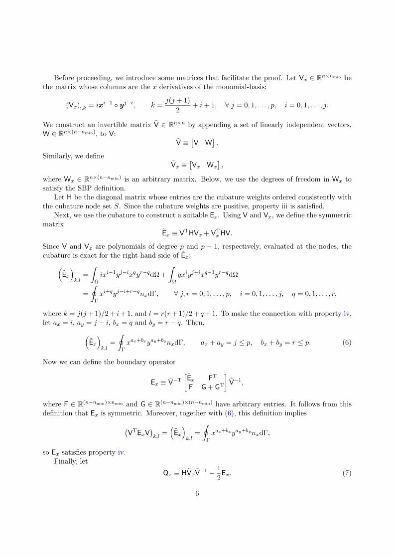
Before proceeding, we introduce some matrices that facilitate the proof. Let Vx ∈ Rn×nmin bethe matrix whose columns are the x derivatives of the monomial-basis:

(Vx):,k = ixi−1 yj−i, k =j(j + 1)

2+ i+ 1, ∀ j = 0, 1, . . . , p, i = 0, 1, . . . , j.

We construct an invertible matrix V ∈ Rn×n by appending a set of linearly independent vectors,W ∈ Rn×(n−nmin), to V:

V ≡[V W

].

Similarly, we defineVx ≡

[Vx Wx

],

where Wx ∈ Rn×(n−nmin) is an arbitrary matrix. Below, we use the degrees of freedom in Wx tosatisfy the SBP definition.

Let H be the diagonal matrix whose entries are the cubature weights ordered consistently withthe cubature node set S. Since the cubature weights are positive, property iii is satisfied.

Next, we use the cubature to construct a suitable Ex. Using V and Vx, we define the symmetricmatrix

Ex ≡ VTHVx + VTxHV.

Since V and Vx are polynomials of degree p and p − 1, respectively, evaluated at the nodes, thecubature is exact for the right-hand side of Ex:(

Ex

)k,l

=

∫Ωixi−1yj−ixqyr−qdΩ +

∫Ωqxiyj−ixq−1yr−qdΩ

=

∮Γxi+qyj−i+r−qnxdΓ, ∀ j, r = 0, 1, . . . , p, i = 0, 1, . . . , j, q = 0, 1, . . . , r,

where k = j(j+ 1)/2 + i+ 1, and l = r(r+ 1)/2 + q+ 1. To make the connection with property iv,let ax = i, ay = j − i, bx = q and by = r − q. Then,(

Ex

)k,l

=

∮Γxax+bxyay+bynxdΓ, ax + ay = j ≤ p, bx + by = r ≤ p. (6)

Now we can define the boundary operator

Ex ≡ V−T

[Ex FT

F G + GT

]V−1,

where F ∈ R(n−nmin)×nmin and G ∈ R(n−nmin)×(n−nmin) have arbitrary entries. It follows from thisdefinition that Ex is symmetric. Moreover, together with (6), this definition implies

(VTExV

)k,l

=(Ex

)k,l

=

∮Γxax+bxyay+bynxdΓ,

so Ex satisfies property iv.Finally, let

Qx ≡ HVxV−1 − 1

2Ex. (7)

6

The accuracy conditions, which are equivalent to showing DxV = Vx, follow immediately from thisdefinition of Qx:

DxV = H−1

(Qx +

1

2Ex

)V = H−1

(HVxV

−1)V = Vx,

thus, property i is satisfied.Our remaining task is to show that Qx can be constructed to be antisymmetric; inspecting (7),

we see that the Wx block of Vx provides the only available degrees of freedom to achieve this task.If we can show that

VTQxV =

[VTQxV VTQxWWTQxV WTQxW

]can be made antisymmetric, then the result will follow for Qx. Consider the first block in the 2× 2block matrix above, i.e.

VTQxV = VTHVx −1

2VTExV.

Adding this block to its transpose, we find

VTQxV + VTQTxV = VTHVx + VT

xHV − VTExV, (8)

where we have used the symmetry of Ex. The right-hand side of (8) is the matrix form of the(rearranged) compatibility equations (5). Thus, VTQxV+VTQT

xV = 0, proving that the first blockis antisymmetric. For the remaining three blocks, antisymmetry requires(

VTQxW)T

= −WTQxV, and WTQxW = −WTQTxW.

Substituting Qx and simplifying, we obtain the following equations for the unknown Wx:

VTHWx = −VTxHW + VTExW, and WTHWx + WT

xHW = WTExW.

The first matrix equation constitutes nmin(n − nmin) scalar equations, while the second equationholds (n − nmin)2 scalar equations. Therefore, there are n(n − nmin) equations in total. This isprecisely the number of degrees of freedom in Wx. Therefore, by choosing those values for Wx thatsatisfy the matrix equations above, we ensure the antisymmetry of Qx.

Remark 1. For a given cubature rule, we have shown existence but not uniqueness of an SBPoperator. In the proof of Theorem 2, all of the degrees of freedom in Wx were used to satisfy theantisymmetry of Qx; however, we did not use any of the freedom in the matrices F and G found inEx. Therefore, in general, there are infinitely many operators associated with a given cubature rulethat satisfy Definition 1.

We now characterize Sx.

Theorem 3. The matrix Sx of a degree p diagonal-norm multi-dimensional SBP operator is adegree τSx = min (τEx , 2p) approximation to the bilinear form

(V,U) =

∫ΩV ∂U∂x

dΩ (9)

Proof. The proof is analogous to the proof in [20] for one-dimensional classical finite-difference-SBPoperators.

7

Using Theorem (3) we can characterize Qx as follows:

Theorem 4. The matrix Qx of a degree p diagonal-norm multi-dimensional SBP operator is adegree τQx = min (τEx , 2p) approximation to the bilinear form

(V,U) =

∫ΩV ∂U∂x

dΩ− 1

2

∮ΓVUdΓ (10)

Proof. By Theorem (3) we have that(xbx yby

)TSxx

ax yay =

∫Ωxbxyby

∂xaxyay

∂xdΩ,

∀ ax + ay + bx + by ≤ min (τEx , 2p) .

(11)

Substituting Sx = Qx + 12Ex into (11), with rearrangement, gives

(xbx yby

)TQxx

ax yay =

∫Ωxbxyby

∂xaxyay

∂xdΩ− 1

2

(xbx yby

)TExx

ax yay ,

∀ ax + ay + bx + by ≤ min (τEx , 2p) .

(12)

Using the definition of Ex we get the desired result(xbx yby

)TQxx

ax yay =

∫Ωxbxyby

∂xaxyay

∂xdΩ− 1

2

∮ΓxaxyayxbxybydΓ,

∀ ax + ay + bx + by ≤ min (τEx , 2p) .

(13)

4. Constructing the operators

This section describes how we construct diagonal-norm SBP operators for triangles and tetra-hedrons. The algorithms described below have been implemented in the Julia package Summa-tionByParts5.

4.1. The node coordinates and the norm matrix

Theorem 1 tells us that the diagonal entries in H are positive weights from a cubature that isexact for polynomials of total degree 2p − 1. Thus, our first task is to find cubature rules withpositive weights for the triangle and tetrahedron. Additionally, we seek rules that use as few nodesas possible for a given accuracy and that respect the symmetries of the triangle and tetrahedron.

For the operators considered in this work, we require that(p+d−1d−1

)cubature nodes lie on each

boundary facet, where d is the spatial dimension. This requirement on the nodes is motivated bythe particular form of the Ex, Ey, and Ez operators that we consider below; however, Definition1 does not require a prescribed number of boundary nodes, and SBP operators for the 2- and3-simplex may exist that do not have any boundary nodes at all.

5https://github.com/OptimalDesignLab/SummationByParts.jl

8

Table 1: Active orbits and their node counts for triangular-element operators. The notation Perm indicates thatevery permutation of the barycentric coordinates is to be considered. Free-node counts are decomposed into theproduct of the number of nodes in the orbit times the number of orbits of that type.

operator degree, p

orbit name barycentric form 1 2 3 4

fixed nodes vertices Perm(1, 0, 0) 3 3 3 3

mid-edge Perm(

12 ,

12 , 0)

— 3 — 3

centroid(

13 ,

13 ,

13

)— 1 — —

free nodes edge Perm (α, 1− α, 0) — — 6× 1 6× 1

S21 Perm (α, α, 1− 2α) — — 3× 1 3× 2

# free parameters — — 2 3# nodes total 3 7 12 18

p = 1 p = 2 p = 3 p = 4

Figure 1: Node distributions for cubature rules adopted for the SBP operators on triangles.

Cubature rules that meet our requirements for triangular elements are presented in refer-ences [21–23, 25] in the context of the spectral-element and spectral-difference methods. Table 1summarizes the rules that are adopted for triangular-element SBP operators of degree p = 1, 2, 3,and 4. For reference, the node locations for the triangular cubature rules are shown in Figure 1.

To find cubature rules for the tetrahedron, we follow the ideas presented in [23, 26, 27]. Ourprocedure is briefly outlined below for completeness, but we make no claims regarding the noveltyof the cubature rules or our method of finding them.

We assume that each node belongs to a (possibly degenerate) symmetry orbit [26]. As indicatedabove, we assume that the cubature-node set includes p+1 nodes along each edge and (p+1)(p+2)/2nodes on each triangular face. For the interior nodes, we activate the minimum number of symmetryorbits necessary to satisfy the accuracy conditions; these orbits have been identified through trial-and-error.

Each symmetry orbit has a cubature weight associated with it, and orbits that are non-degenerate are parameterized using one or more barycentric parameters. Together, the orbitparameters and the weights are the degrees of freedom that must be determined. They arefound by solving the nonlinear accuracy conditions using the Levenberg-Marquardt algorithm.

9

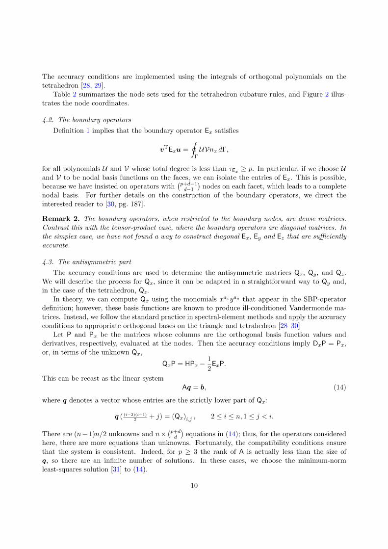
The accuracy conditions are implemented using the integrals of orthogonal polynomials on thetetrahedron [28, 29].

Table 2 summarizes the node sets used for the tetrahedron cubature rules, and Figure 2 illus-trates the node coordinates.

4.2. The boundary operators

Definition 1 implies that the boundary operator Ex satisfies

vTExu =

∮ΓUVnx dΓ,

for all polynomials U and V whose total degree is less than τEx ≥ p. In particular, if we choose Uand V to be nodal basis functions on the faces, we can isolate the entries of Ex. This is possible,because we have insisted on operators with

(p+d−1d−1

)nodes on each facet, which leads to a complete

nodal basis. For further details on the construction of the boundary operators, we direct theinterested reader to [30, pg. 187].

Remark 2. The boundary operators, when restricted to the boundary nodes, are dense matrices.Contrast this with the tensor-product case, where the boundary operators are diagonal matrices. Inthe simplex case, we have not found a way to construct diagonal Ex, Ey and Ez that are sufficientlyaccurate.

4.3. The antisymmetric part

The accuracy conditions are used to determine the antisymmetric matrices Qx, Qy, and Qz.We will describe the process for Qx, since it can be adapted in a straightforward way to Qy and,in the case of the tetrahedron, Qz.

In theory, we can compute Qx using the monomials xaxyay that appear in the SBP-operatordefinition; however, these basis functions are known to produce ill-conditioned Vandermonde ma-trices. Instead, we follow the standard practice in spectral-element methods and apply the accuracyconditions to appropriate orthogonal bases on the triangle and tetrahedron [28–30]

Let P and Px be the matrices whose columns are the orthogonal basis function values andderivatives, respectively, evaluated at the nodes. Then the accuracy conditions imply DxP = Px,or, in terms of the unknown Qx,

QxP = HPx −1

2ExP.

This can be recast as the linear systemAq = b, (14)

where q denotes a vector whose entries are the strictly lower part of Qx:

q ( (i−2)(i−1)2

+ j) = (Qx)i,j , 2 ≤ i ≤ n, 1 ≤ j < i.

There are (n− 1)n/2 unknowns and n×(p+dd

)equations in (14); thus, for the operators considered

here, there are more equations than unknowns. Fortunately, the compatibility conditions ensurethat the system is consistent. Indeed, for p ≥ 3 the rank of A is actually less than the size ofq, so there are an infinite number of solutions. In these cases, we choose the minimum-normleast-squares solution [31] to (14).

10

Table 2: Active orbits and their node counts for tetrahedral-element operators. See the caption of Table 1 for anexplanation of the notation.

operator degree, p

orbit name barycentric form 1 2 3 4

fixed nodes vertices Perm(1, 0, 0, 0) 4 4 4 4

mid-edge Perm(

12 ,

12 , 0, 0

)— 6 — 6

centroid(

14 ,

14 ,

14 ,

14

)— 1 — 1

face centroid Perm(

13 ,

13 ,

13 , 0)

— — 4 —

free nodes edge Perm (α, 1− α, 0, 0) — — 12× 1 12× 1

face S21 Perm (α, α, 1− 2α, 0) — — — 12× 1

S31 Perm (α, α, α, 1− 3α) — — 4× 1 4× 1

S22 Perm(α, α, 1

2 − α,12 − α

)— — — 6× 1

# free parameters — — 2 4# nodes total 4 11 24 45

p = 1 p = 2 p = 3 p = 4

Figure 2: Node distributions for cubature rules adopted for the SBP operators on tetrahedra.

4.4. Similarities and differences with existing operators

There is a vast literature on high-order discretizations for simplex elements, so we focus on thetwo that share the most in common with the proposed SBP operators: the diagonal mass-matrixspectral-element (SE) method [21–23] and the spectral-difference (SD) method [32].

Our norm matrix H is identical to the lumped mass matrices in the SE method. The differencebetween the methods arises in the definition of Sx. In the SE method of Giraldo and Taylor [23],the Sx matrix is defined as

(SSEx

)i,j

=

n∑k=0

Hk,kφi(xk, yk)∂φj∂x

(xk, yk),

where φini=1 is the so-called cardinal basis. For a degree p operator, the cardinal basis is a

11

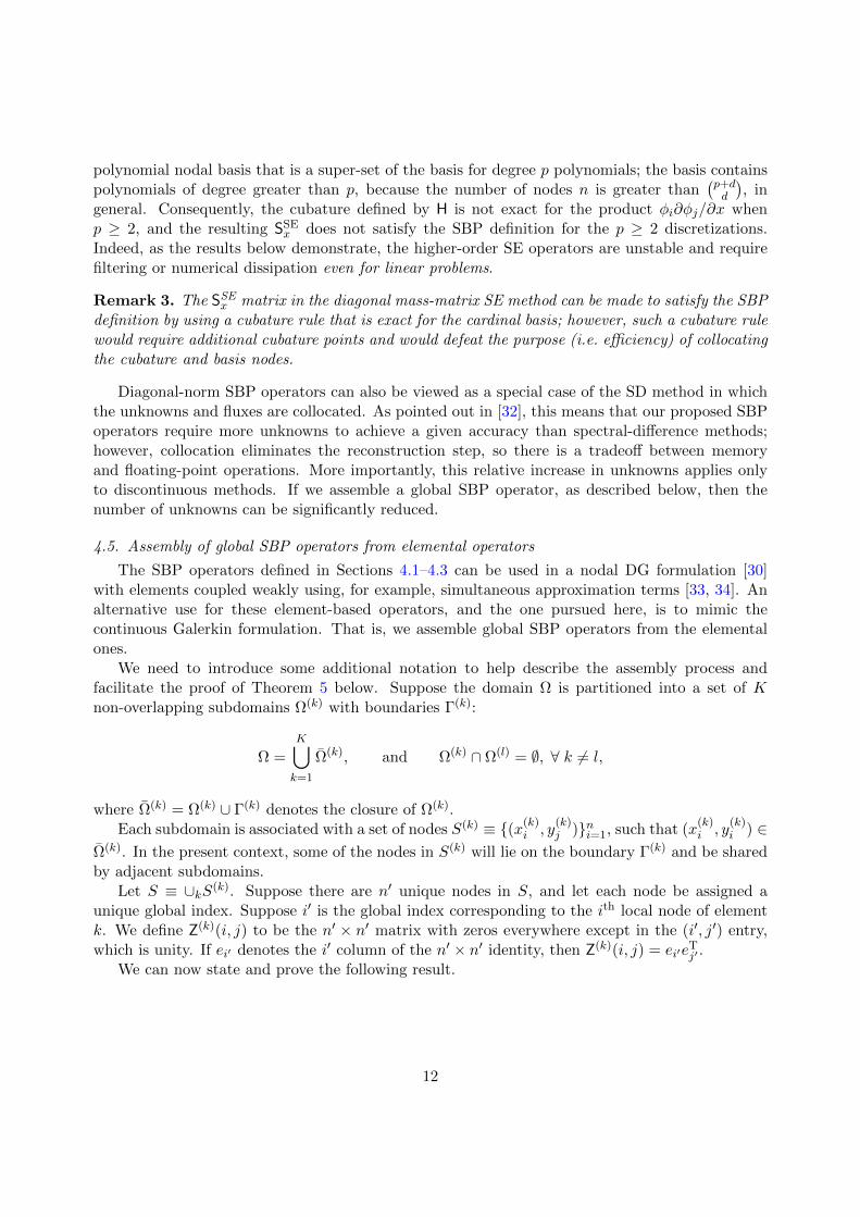
polynomial nodal basis that is a super-set of the basis for degree p polynomials; the basis containspolynomials of degree greater than p, because the number of nodes n is greater than

(p+dd

), in

general. Consequently, the cubature defined by H is not exact for the product φi∂φj/∂x whenp ≥ 2, and the resulting SSE

x does not satisfy the SBP definition for the p ≥ 2 discretizations.Indeed, as the results below demonstrate, the higher-order SE operators are unstable and requirefiltering or numerical dissipation even for linear problems.

Remark 3. The SSEx matrix in the diagonal mass-matrix SE method can be made to satisfy the SBPdefinition by using a cubature rule that is exact for the cardinal basis; however, such a cubature rulewould require additional cubature points and would defeat the purpose (i.e. efficiency) of collocatingthe cubature and basis nodes.

Diagonal-norm SBP operators can also be viewed as a special case of the SD method in whichthe unknowns and fluxes are collocated. As pointed out in [32], this means that our proposed SBPoperators require more unknowns to achieve a given accuracy than spectral-difference methods;however, collocation eliminates the reconstruction step, so there is a tradeoff between memoryand floating-point operations. More importantly, this relative increase in unknowns applies onlyto discontinuous methods. If we assemble a global SBP operator, as described below, then thenumber of unknowns can be significantly reduced.

4.5. Assembly of global SBP operators from elemental operators

The SBP operators defined in Sections 4.1–4.3 can be used in a nodal DG formulation [30]with elements coupled weakly using, for example, simultaneous approximation terms [33, 34]. Analternative use for these element-based operators, and the one pursued here, is to mimic thecontinuous Galerkin formulation. That is, we assemble global SBP operators from the elementalones.

We need to introduce some additional notation to help describe the assembly process andfacilitate the proof of Theorem 5 below. Suppose the domain Ω is partitioned into a set of Knon-overlapping subdomains Ω(k) with boundaries Γ(k):

Ω =K⋃k=1

Ω(k), and Ω(k) ∩ Ω(l) = ∅, ∀ k 6= l,

where Ω(k) = Ω(k) ∪ Γ(k) denotes the closure of Ω(k).Each subdomain is associated with a set of nodes S(k) ≡ (x(k)

i , y(k)j )ni=1, such that (x

(k)i , y

(k)i ) ∈

Ω(k). In the present context, some of the nodes in S(k) will lie on the boundary Γ(k) and be sharedby adjacent subdomains.

Let S ≡ ∪kS(k). Suppose there are n′ unique nodes in S, and let each node be assigned aunique global index. Suppose i′ is the global index corresponding to the ith local node of elementk. We define Z(k)(i, j) to be the n′ × n′ matrix with zeros everywhere except in the (i′, j′) entry,which is unity. If ei′ denotes the i′ column of the n′ × n′ identity, then Z(k)(i, j) = ei′e

Tj′ .

We can now state and prove the following result.

12

Theorem 5. Let D(k)x =

(H(k)

)−1S

(k)x be a degree p SBP operator for the first derivative ∂/∂x on

the node set S(k). If

H ≡K∑k=1

n∑i=1

H(k)i,i Z

(k)(i, i)

Sx ≡K∑k=1

n∑i=1

n∑j=1

(S(k)x

)i,j

Z(k)(i, j),

then Dx = H−1Sx is a degree p SBP operator on the global node set S.

Proof. We need to check each of the four properties in Definition 1.

i) The first property is straightforward, albeit tedious, to verify. H−1 exists by property iii, whichis shown to hold independently below, so we have

Dxxax yay = H−1Sxx

ax yay

= H−1

K∑k=1

n∑i=1

n∑j=1

(S(k)x

)i,j

Z(k)(i, j)

xax yay

= H−1K∑k=1

n∑i=1

H(k)i,i

H(k)i,i

n∑j=1

(S(k)x

)i,jei′x

axj′ y

ayj′

= H−1K∑k=1

n∑i=1

H(k)i,i ei′

n∑j=1

(D(k)x

)i,jxaxj y

ayj

= H−1K∑k=1

n∑i=1

H(k)i,i ei′axx

ax−1i y

ayi

= H−1

[K∑k=1

n∑i=1

H(k)i,i Z

(k)(i, i)

]axx

ax−1yay ,

But the term in brackets above is the definition of H, so we are left with Dxxax yay =

axxax−1yay , as desired.

ii) We form the decomposition Sx = Qx + 12Ex where

Qx =K∑k=1

n∑i=1

n∑j=1

(Qx)(k) (i, j)Z(k)i,j ,

Ex =K∑k=1

n∑i=1

n∑j=1

E(k)x (i, j)Z

(k)i,j .

The matrix Qx is antisymmetric, because it is the sum of antisymmetric matrices. Similarly,Ex is symmetric, because it is the sum of symmetric matrices. Hence, property ii is satisfied.

iii) H is clearly diagonal and positive by construction, so property iii is satisfied.

13

iv) Finally, property iv can be verified through direct evaluation:

(xax yay)T Exxbx yby =

K∑k=1

n∑i=1

n∑j=1

E(k)x (i, j) (xax yay)Z

(k)i,j x

bx yby

=

K∑k=1

∮Γ(k)

xax+bxyay+bynxdΓ

=

∮Γxax+bxyay+bynxdΓ,

where we have used the fact that the boundary fluxes of adjacent elements cancel analytically.

5. Results

The linear advection equation is used to verify and study the triangular-element SBP operatorsof Section 4. In particular, we consider the problem

∂U∂t

+∂U∂x

+∂U∂y

= 0, ∀ (x, y) ∈ Ω = [0, 1]2,

U(x, 0, t) = U(x, 1, t), and U(0, y, t) = U(1, y, t),

U(x, y, 0) =

1− (4r2 − 1)5 if r ≤ 1

2

1, otherwise,

where r(x, y) ≡√

(x− 12)2 + (y − 1

2)2. The boundary conditions imply periodicity in both the x

and y directions and the PDE implies an advection velocity of (1, 1). The initial condition is a C4

continuous bump function that is periodic on Ω.A nonuniform mesh for the square domain Ω is generated, in order to eliminate possible error

cancellations that may arise on uniform grids. The vertices of the mesh are given by

xi,j =i

N+

1

40sin (2πi/N) sin (2πj/N) , yi,j =

j

N+

1

40sin (2πi/N) sin (2πj/N) ,

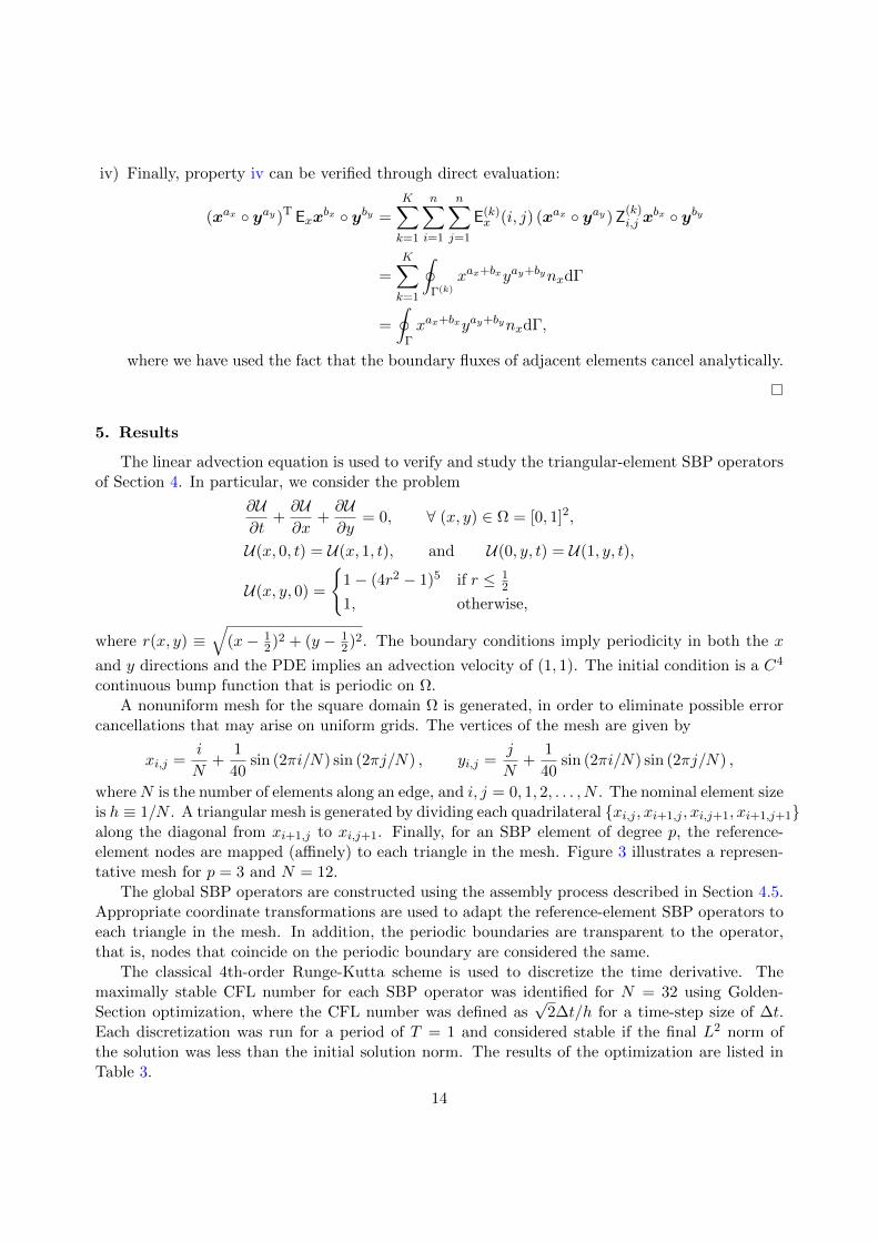
whereN is the number of elements along an edge, and i, j = 0, 1, 2, . . . , N . The nominal element sizeis h ≡ 1/N . A triangular mesh is generated by dividing each quadrilateral xi,j , xi+1,j , xi,j+1, xi+1,j+1along the diagonal from xi+1,j to xi,j+1. Finally, for an SBP element of degree p, the reference-element nodes are mapped (affinely) to each triangle in the mesh. Figure 3 illustrates a represen-tative mesh for p = 3 and N = 12.

The global SBP operators are constructed using the assembly process described in Section 4.5.Appropriate coordinate transformations are used to adapt the reference-element SBP operators toeach triangle in the mesh. In addition, the periodic boundaries are transparent to the operator,that is, nodes that coincide on the periodic boundary are considered the same.

The classical 4th-order Runge-Kutta scheme is used to discretize the time derivative. Themaximally stable CFL number for each SBP operator was identified for N = 32 using Golden-Section optimization, where the CFL number was defined as

√2∆t/h for a time-step size of ∆t.

Each discretization was run for a period of T = 1 and considered stable if the final L2 norm ofthe solution was less than the initial solution norm. The results of the optimization are listed inTable 3.

14

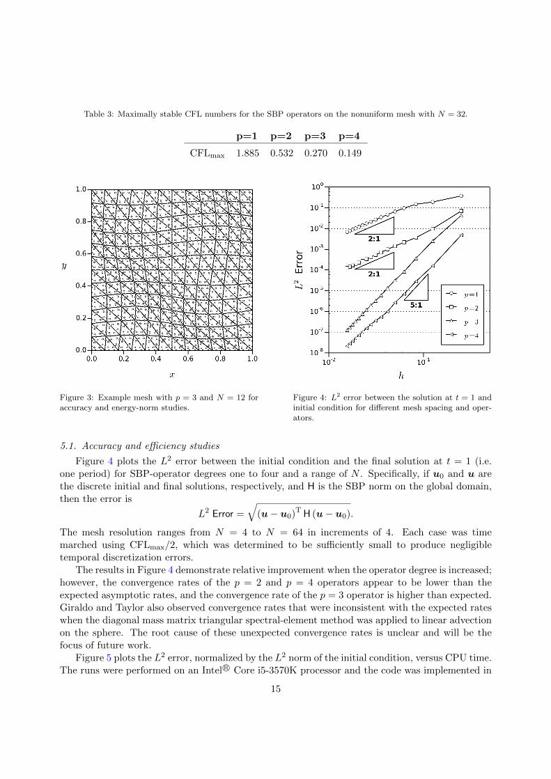
Table 3: Maximally stable CFL numbers for the SBP operators on the nonuniform mesh with N = 32.

p=1 p=2 p=3 p=4

CFLmax 1.885 0.532 0.270 0.149

Figure 3: Example mesh with p = 3 and N = 12 foraccuracy and energy-norm studies.

Figure 4: L2 error between the solution at t = 1 andinitial condition for different mesh spacing and oper-ators.

5.1. Accuracy and efficiency studies

Figure 4 plots the L2 error between the initial condition and the final solution at t = 1 (i.e.one period) for SBP-operator degrees one to four and a range of N . Specifically, if u0 and u arethe discrete initial and final solutions, respectively, and H is the SBP norm on the global domain,then the error is

L2 Error =

√(u− u0)T H (u− u0).

The mesh resolution ranges from N = 4 to N = 64 in increments of 4. Each case was timemarched using CFLmax/2, which was determined to be sufficiently small to produce negligibletemporal discretization errors.

The results in Figure 4 demonstrate relative improvement when the operator degree is increased;however, the convergence rates of the p = 2 and p = 4 operators appear to be lower than theexpected asymptotic rates, and the convergence rate of the p = 3 operator is higher than expected.Giraldo and Taylor also observed convergence rates that were inconsistent with the expected rateswhen the diagonal mass matrix triangular spectral-element method was applied to linear advectionon the sphere. The root cause of these unexpected convergence rates is unclear and will be thefocus of future work.

Figure 5 plots the L2 error, normalized by the L2 norm of the initial condition, versus CPU time.The runs were performed on an Intel R© Core i5-3570K processor and the code was implemented in

15

Figure 5: Normalized L2 error at T = 1 versus CPU time measured in seconds.

Julia version 0.4.0. For this problem, the p = 2 SBP discretization is the most efficient over therange of accuracies typical of engineering applications. When the desired relative accuracy is below0.3%, the p = 4 discretization is the most efficient. These results are typical of other high-orderdiscretizations applied to linear convection.

5.2. Stability studies

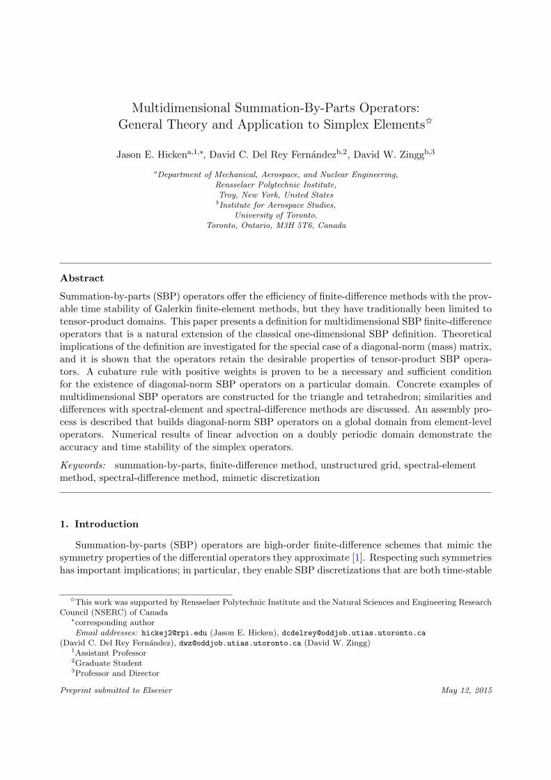
Figure 6 shows the spectra of the SBP and SE spatial operators for the linear advection problem.Specifically, these eigenvalues are for the global operator Sx +Sy when N = 12. The eigenvalues ofthe SBP operators are imaginary to machine precision, which mimics the continuous spectrum for

this periodic problem. This is as expected, because the boundary operators E(k)x cancel between

adjacent elements when the SBP derivative operator is assembled, leaving only the antisymmetricparts. The SE operator for p = 1 also has a purely imaginary spectrum, because it is identical to thelinear SBP operator; however, the spectra of the high-order SE operators have a real component.

The consequences of the eigenvalue distributions are evident when the linear advection problemis integrated for two periods. Figure 7 plots the difference between the solution L2 norm at timet ∈ [0, 2] and the initial solution norm, i.e. the change in “energy”,

∆E = uTnHun − uT

0 Hu0,

where un denotes the discrete solution at time step n. For this study, N = 12 and the CFL numberwas fixed at 0.01 to reduce temporal errors.

The energy history in Figure 7 clearly shows that the SE operators are unstable for this linearadvection problem, while the SBP operators are stable. The small (linear) decrease in the SBPenergy error is due to temporal errors and can be eliminated by using a different time-marchingmethod, e.g. leapfrog, or at the cost of using a sufficiently small CFL number.

6. Conclusions

We proposed a definition for multidimensional SBP operators that is a natural extension of theclassical one-dimensional SBP operator definition. We studied the theoretical implications of the

16

p = 1 (SBP) p = 2 (SBP) p = 3 (SBP) p = 4 (SBP)

p = 1 (SE) p = 2 (SE) p = 3 (SE) p = 4 (SE)

Figure 6: Eigenvalue distributions for the SBP (upper row) and the SE (lower row) spatial discretizations of thelinear advection problem. Note the different ranges for the real variables.

Figure 7: Time history of the change in the solution energy norm. Note the use of a symmetric logarithmic scale onthe vertical axis.

17

definition in the case of diagonal-norm operators, and showed that the generalized operators retainthe attractive properties of tensor-product SBP operators. A significant theoretical result of thiswork is that, for a given domain, a cubature rule with positive weights is necessary and sufficientfor the existence of diagonal-norm SBP operators on that domain.

We also constructed diagonal-norm SBP operators for the triangle and tetrahedron. To thebest of our knowledge, this is the first example of SBP operators of degree p ≥ 2 on these domains.We also presented an assembly procedure that constructs SBP operators for a global domain fromelement-wise SBP operators.

Finally, we verified the triangle-element SBP operators using linear advection on a doublyperiodic domain. The results demonstrate the time stability and accuracy of the operators. Theresults suggest these operators could be effective for the long-time simulation of turbulent flows oncomplex domains.

Acknowledgments

J. E. Hicken acknowledges the financial support of Rensselaer Polytechnic Institute, and D. W. Zinggacknowledges the support of the Natural Sciences and Engineering Research Council (NSERC) ofCanada.

All figures were produced using Matplotlib [35].

References

[1] Kreiss, H.-O. and Scherer, G., “Finite element and finite difference methods for hyperbolic partial differen-tial equations,” Mathematical aspects of finite elements in partial differential equations, Academic Press, NewYork/London, 1974, pp. 195–212.

[2] Carpenter, M. H., Nordstrom, J., and Gottlieb, D., “A stable and conservative interface treatment of arbitraryspatial accuracy,” Journal of Computational Physics, Vol. 148, No. 2, 1999, pp. 341–365.

[3] Yee, H. C. and Sjogreen, B., “Designing adaptive low-dissipative high order schemes for long-time integrations,”Turbulent Flow Computation, Springer, 2002, pp. 141–198.

[4] Nordstrom, J., “Conservative finite difference formulations, variable coefficients, energy estimates and artificialdissipation,” Journal of Scientific Computing , Vol. 29, 2006, pp. 375–404.

[5] Morinishi, Y., Lund, T. S., Vasilyev, O. V., and Moin, P., “Fully Conservative Higher Order Finite DifferenceSchemes for Incompressible Flow,” Journal of Computational Physics, Vol. 143, 1998, pp. 90–124.

[6] Yee, H. C., Vinokur, M., and Djomehri, M. J., “Entropy Splitting and Numerical Dissipation,” Journal ofComputational Physics, Vol. 162, No. 1, July 2000, pp. 33–81.

[7] Strand, B., “Summation by parts for finite difference approximations for d/dx,” Journal of ComputationalPhysics, Vol. 110, No. 1, 1994, pp. 47–67.

[8] Mattsson, K. and Nordstrom, J., “Summation by parts operators for finite difference approximations of secondderivatives,” Journal of Computational Physics, Vol. 199, No. 2, 2004, pp. 503–540.

[9] Svard, M., “On coordinate transformations for summation-by-parts operators,” Journal of Scientific Computing ,Vol. 20, No. 1, Feb. 2004, pp. 29–42.

[10] Mattsson, K., “Summation by Parts Operators for Finite Difference Approximations of Second-Derivatives withVariable Coefficients,” Journal of Scientific Computing , Vol. 51, No. 3, June 2012, pp. 650–682.

[11] Svard, M., Mattsson, K., and Nordstrom, J., “Steady-State Computations Using Summation-by-Parts Opera-tors,” Journal of Scientific Computing , Vol. 24, No. 1, July 2005, pp. 79–95.

[12] Hicken, J. E. and Zingg, D. W., “A parallel Newton-Krylov solver for the Euler equations discretized usingsimultaneous approximation terms,” AIAA Journal , Vol. 46, No. 11, Nov. 2008, pp. 2773–2786.

[13] Nordstrom, J., Gong, J., van der Weide, E., and Svard, M., “A stable and conservative high order multi-blockmethod for the compressible Navier-Stokes equations,” Journal of Computational Physics, Vol. 228, No. 24,2009, pp. 9020–9035.

[14] Kitson, A., McLachlan, R. I., and Robidoux, N., “Skew-adjoint finite difference methods on nonuniform grids,”New Zealand Journal of Mathematics, Vol. 32, No. 2, 2003, pp. 139–159.

18

[15] Kwan-yu Chiu, E., Wang, Q., Hu, R., and Jameson, A., “A Conservative Mesh-Free Scheme and General-ized Framework for Conservation Laws,” SIAM Journal on Scientific Computing , Vol. 34, No. 6, Jan. 2012,pp. A2896–A2916.

[16] Chiu, E. K., Wang, Q., and Jameson, A., “A conservative meshless scheme: general order formulation andapplication to Euler equations,” 49th AIAA Aerospace Sciences Meeting , No. AIAA–2011–651, Orlando, Florida,Jan. 2011.

[17] Carpenter, M. H. and Gottlieb, D., “Spectral methods on arbitrary grids,” Journal of Computational Physics,Vol. 129, No. 1, 1996, pp. 74–86.

[18] Gassner, G. J., “A skew-symmetric discontinuous Galerkin spectral element discretization and its relation toSBP-SAT finite difference methods,” SIAm Journal on Scientific Computing , Vol. 35, No. 3, 2013, pp. A1233–A1253.

[19] Del Rey Fernandez, D. C., Boom, P. D., and Zingg, D. W., “A Generalized Framework for Nodal First DerivativeSummation-By-Parts Operators,” Journal of Computational Physics, Vol. 266, No. 1, 2014, pp. 214–239.

[20] Hicken, J. E. and Zingg, D. W., “Summation-by-parts operators and high-order quadrature,” Journal of Com-putational and Applied Mathematics, Vol. 237, No. 1, 2013, pp. 111–125.

[21] Cohen, G., Joly, P., Roberts, J. E., and Tordjman, N., “Higher Order Triangular Finite Elements with MassLumping for the Wave Equation,” SIAM Journal on Numerical Analysis, Vol. 38, No. 6, Jan. 2001, pp. 2047–2078.

[22] Mulder, W. A., “Higher-order mass-lumped finite elements for the wave equation,” Journal of ComputationalAcoustics, Vol. 09, No. 02, June 2001, pp. 671–680.

[23] Giraldo, F. X. and Taylor, M. A., “A diagonal-mass-matrix triangular-spectral-element method based on cuba-ture points,” Journal of Engineering Mathematics, Vol. 56, No. 3, 2006, pp. 307–322.

[24] Hicken, J. E. and Zingg, D. W., “Dual consistency and functional accuracy: a finite-difference perspective,”Journal of Computational Physics, Vol. 256, Jan. 2014, pp. 161–182.

[25] Liu, Y. and Vinokur, M., “Exact Integrations of Polynomials and Symmetric Quadrature Formulas over Arbi-trary Polyhedral Grids,” Journal of Computational Physics, Vol. 140, No. 1, 1998, pp. 122–147.

[26] Zhang, L., Cui, T., and Liu, H., “A Set of Symmetric Quadrature Rules on Triangles and Tetrahedra,” Journalof Computational Mathematics, Vol. 27, No. 1, 2009, pp. 89–96.

[27] Witherden, F. D. and Vincent, P. E., “On the Identification of Symmetric Quadrature Rules for Finite ElementMethods,” Sept. 2014.

[28] Koornwinder, T., “Two-variable analogues of the classical orthogonal polynomials,” Theory and application ofspecial functions, Academic Press New York, 1975, pp. 435–495.

[29] Dubiner, M., “Spectral methods on triangles and other domains,” Journal of Scientific Computing , Vol. 6, No. 4,1991, pp. 345–390.

[30] Hesthaven, J. S. and Warburton, T., Nodal discontinuous Galerkin methods: algorithms, analysis, and applica-tions, Springer-Verlag, New York, 2008.

[31] Golub, G. H. and Van Loan, C. F., Matrix Computations, The John Hopkins University Press, 3rd ed., 1996.[32] Liu, Y., Vinokur, M., and Wang, Z. J., “Spectral difference method for unstructured grids I: Basic formulation,”

Journal of Computational Physics, Vol. 216, No. 2, Aug. 2006, pp. 780–801.[33] Funaro, D. and Gottlieb, D., “A new method of imposing boundary conditions in pseudospectral approximations

of hyperbolic equations,” Mathematics of Computation, Vol. 51, No. 184, Oct. 1988, pp. 599–613.[34] Carpenter, M. H., Gottlieb, D., and Abarbanel, S., “Time-stable boundary conditions for finite-difference

schemes solving hyperbolic systems: Methodology and application to high-order compact schemes,” Journalof Computational Physics, Vol. 111, No. 2, 1994, pp. 220–236.

[35] Hunter, J. D., “Matplotlib: A 2D graphics environment,” Computing In Science & Engineering , Vol. 9, No. 3,2007, pp. 90–95.

19