Embed Size (px)
Citation preview

Multidimensional Signal Processing
Mark Eisen, Alec Koppel, and Alejandro Ribeiro
Dept. of Electrical and Systems EngineeringUniversity of [email protected]
http://www.seas.upenn.edu/users/~aribeiro/
March 15, 2018
Signal and Information Processing Multidimensional Signal Processing 1
Signal representation
Signal representation
Images
Two dimensional discrete signals
Two dimensional (2D) discrete Fourier transform (DFT)
Two dimensional (2D) inverse (i) discrete Fourier transform (DFT)
Energy conservation (Parseval’s theorem)
Convolution in 2 dimensions
Applications
Discrete Cosine Transform
2D Discrete Cosine Transform
JPEG image compression
Signal and Information Processing Multidimensional Signal Processing 2
It’s all oh so simple
I Once and again, things are invisible or obscure in time domain
⇒ But they become visible and clear in the frequency domain
I Even when clear in time, they are easier to understand in frequency
I Literally a new sense to view things that are otherwise invisible
“On ne voit bien qu’avec le coeur.L’essentiel est invisible pour les yeux.”
The Little Prince
I One sees clearly only with the frequency
The essential is invisible to the eyes
Signal and Information Processing Multidimensional Signal Processing 3
Signal representation
I Why a new sense? ⇒ We can write signals as sums of shifted deltas
x(n) =N∑
k=1
x(k)δ(k − n) (1)
I Conceptually, the same as writing signals as sums of oscillations
x(n) =N∑
k=1
X (k)e j2πkn/N (2)
I Only difference is that we sense time but we don’t sense frequency
I We say we change the signal representation or we change the basis
I It all hinges in our ability to represent the signal in a different domain
Signal and Information Processing Multidimensional Signal Processing 4
Moving forward
I If something is obscure in time but also obscure in frequency
⇒ Change the representation ≡ Change the basis
I Images ⇒ multidimensional DFT, Discrete cosine transform (DCT)
I Stochastic processes ⇒ Principal component analysis (PCA)
⇒ Eigenvectors of the correlation matrix
I Signals defined on graphs ⇒ Graph signal processing
⇒ Eigenvalues of the graph Laplacian
Signal and Information Processing Multidimensional Signal Processing 5
Images
Signal representation
Images
Two dimensional discrete signals
Two dimensional (2D) discrete Fourier transform (DFT)
Two dimensional (2D) inverse (i) discrete Fourier transform (DFT)
Energy conservation (Parseval’s theorem)
Convolution in 2 dimensions
Applications
Discrete Cosine Transform
2D Discrete Cosine Transform
JPEG image compression
Signal and Information Processing Multidimensional Signal Processing 6

Images
I A grid of pixels. Values define the luminescence of the point
⇒ In a black and white image
I In a color image we record multiple channels for different colors
⇒ E.g., red, green, and blue (RGB). Or Yellow Magenta Cyan blacK
I Not unlike signals we studied except that defined over two indices
Signal and Information Processing Multidimensional Signal Processing 7
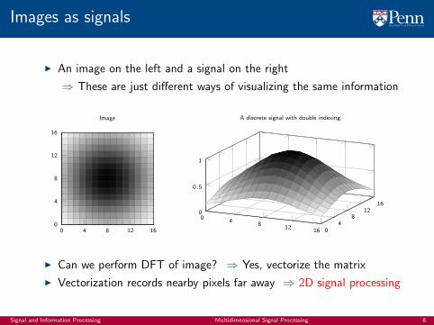
Images as signals
I An image on the left and a signal on the right
⇒ These are just different ways of visualizing the same information
0 4 8 12 160
4
8
12
16
Image
04
812
16 04
812
16
0
0.5
1
A discrete signal with double indexing
I Can we perform DFT of image? ⇒ Yes, vectorize the matrix
I Vectorization records nearby pixels far away ⇒ 2D signal processing
Signal and Information Processing Multidimensional Signal Processing 8
Two dimensional discrete signals
Signal representation
Images
Two dimensional discrete signals
Two dimensional (2D) discrete Fourier transform (DFT)
Two dimensional (2D) inverse (i) discrete Fourier transform (DFT)
Energy conservation (Parseval’s theorem)
Convolution in 2 dimensions
Applications
Discrete Cosine Transform
2D Discrete Cosine Transform
JPEG image compression
Signal and Information Processing Multidimensional Signal Processing 9
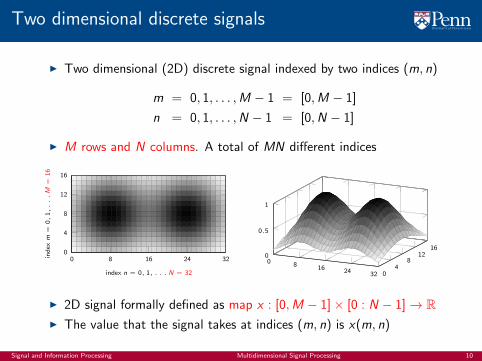
Two dimensional discrete signals
I Two dimensional (2D) discrete signal indexed by two indices (m, n)
m = 0, 1, . . . ,M − 1 = [0,M − 1]
n = 0, 1, . . . ,N − 1 = [0,N − 1]
I M rows and N columns. A total of MN different indices
0 8 16 24 320
4
8
12
16
index n = 0, 1, . . . N = 32
ind
exm
=0,
1,...M
=1
6
0 8 16 24 32 04
812
160
0.5
1
I 2D signal formally defined as map x : [0,M − 1]× [0 : N − 1]→ RI The value that the signal takes at indices (m, n) is x(m, n)
Signal and Information Processing Multidimensional Signal Processing 10
Complex 2D signals
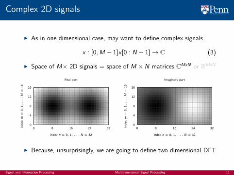
I As in one dimensional case, may want to define complex signals
x : [0,M − 1]x [0 : N − 1]→ C (3)
I Space of M× 2D signals = space of M × N matrices CMxN or RMxN
0 8 16 24 320
4
8
12
16
index n = 0, 1, . . . N = 32
ind
exm
=0,
1,...M
=1
6
Real part
0 8 16 24 320
4
8
12
16
index n = 0, 1, . . . N = 32
ind
exm
=0,
1,...M
=1
6
Imaginary part
I Because, unsurprisingly, we are going to define two dimensional DFT
Signal and Information Processing Multidimensional Signal Processing 11
Deltas in two dimensions
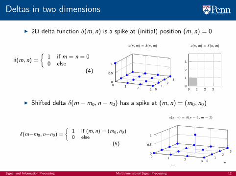
I 2D delta function δ(m, n) is a spike at (initial) position (m, n) = 0
δ(m, n) =
{1 if m = n = 00 else
(4)
0 1 2 3 01
23
0
0.5
1
x(n,m) = δ(n,m)
0 1 2 30
1
2
3
x(n,m) = δ(n,m)
I Shifted delta δ(m −m0, n − n0) has a spike at (m, n) = (m0, n0)
δ(m−m0, n−n0) =
{1 if (m, n) = (m0, n0)0 else
(5)
0 1 2 3 01
23
0
0.5
1
mn
x(n,m) = δ(n − 1,m − 2)
Signal and Information Processing Multidimensional Signal Processing 12
Rectangular pulses
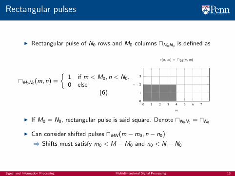
I Rectangular pulse of N0 rows and M0 columns uM0N0 is defined as
uM0N0 (m, n) =
{1 if m < M0, n < N0,0 else
(6)
0 1 2 3 4 5 6 70
1
2
3
m
n
x(n,m) = u24(n,m)
I If M0 = N0, rectangular pulse is said square. Denote uN0N0 = uN0
I Can consider shifted pulses uMN(m −m0, n − n0)
⇒ Shifts must satisfy m0 < M −M0 and n0 < N − N0
Signal and Information Processing Multidimensional Signal Processing 13
Symmetric Gaussian pulses
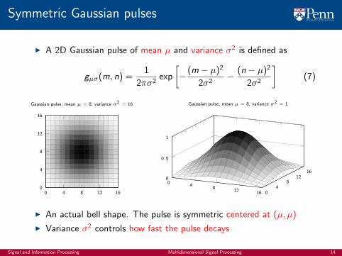
I A 2D Gaussian pulse of mean µ and variance σ2 is defined as
gµσ(m, n) =1
2πσ2exp
[− (m − µ)2
2σ2− (n − µ)2
2σ2
](7)
0 4 8 12 160
4
8
12
16
Gaussian pulse, mean µ = 8, variance σ2 = 16
04
812
16 04
812
16
0
0.5
1
Gaussian pulse, mean µ = 8, variance σ2 = 1
I An actual bell shape. The pulse is symmetric centered at (µ, µ)
I Variance σ2 controls how fast the pulse decays
Signal and Information Processing Multidimensional Signal Processing 14
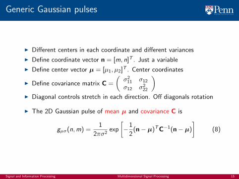
Generic Gaussian pulses
I Different centers in each coordinate and different variances
I Define coordinate vector n = [m, n]T . Just a variable
I Define center vector µ = [µ1, µ2]T . Center coordinates
I Define covariance matrix C =
(σ2
11 σ12
σ12 σ222
)I Diagonal controls stretch in each direction. Off diagonals rotation
I The 2D Gaussian pulse of mean µ and covariance C is
gµσ(n,m) =1
2πσ2exp
[−1
2(n− µ)TC−1(n− µ)
](8)
Signal and Information Processing Multidimensional Signal Processing 15
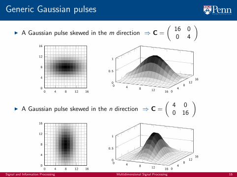
Generic Gaussian pulses
I A Gaussian pulse skewed in the m direction ⇒ C =
(16 00 4
)
0 4 8 12 160
4
8
12
16
0 4 8 12 16 04
812
160
0.5
1
I A Gaussian pulse skewed in the n direction ⇒ C =
(4 00 16
)
0 4 8 12 160
4
8
12
16
0 4 8 12 16 04
812
160
0.5
1
Signal and Information Processing Multidimensional Signal Processing 16
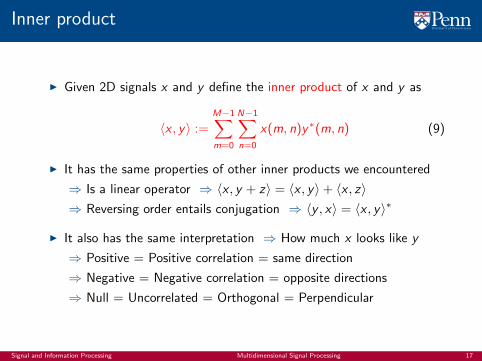
Inner product
I Given 2D signals x and y define the inner product of x and y as
〈x , y〉 :=M−1∑m=0
N−1∑n=0
x(m, n)y∗(m, n) (9)
I It has the same properties of other inner products we encountered
⇒ Is a linear operator ⇒ 〈x , y + z〉 = 〈x , y〉+ 〈x , z〉⇒ Reversing order entails conjugation ⇒ 〈y , x〉 = 〈x , y〉∗
I It also has the same interpretation ⇒ How much x looks like y
⇒ Positive = Positive correlation = same direction
⇒ Negative = Negative correlation = opposite directions
⇒ Null = Uncorrelated = Orthogonal = Perpendicular
Signal and Information Processing Multidimensional Signal Processing 17

Inner product of two rectangular pulses
I The inner product of two square pulses is the number of pixels inwhich both pulses are active (both are one)
0 1 2 3 4 5 6 70
1
2
3
m
n
Inner product of two square pulses
I In the inner product sum 〈x , y〉 =M−1∑m=0
N−1∑n=0
x(m, n)y∗(m, n) only the
terms in which both pulses are not null count
Signal and Information Processing Multidimensional Signal Processing 18

Norm and energy
I The norm of the 2D signal x is ⇒ ‖x‖ :=
[M−1∑m=0
N−1∑n=0
|x(m, n)|2]1/2
I We define the energy of the 2D signal x as the norm squared
‖x‖2 :=M−1∑m=0
N−1∑n=0
|x(m, n)|2 =M−1∑m=0
N−1∑n=0
|xR(m, n)|2+M−1∑m=0
N−1∑n=0
|xI (m, n)|2
(10)
I We can write the energy as self inner product ⇒ ‖x‖2 = 〈x , x〉
Signal and Information Processing Multidimensional Signal Processing 19
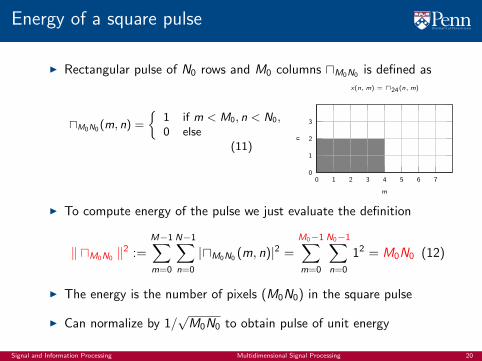
Energy of a square pulse
I Rectangular pulse of N0 rows and M0 columns uM0N0 is defined as
uM0N0 (m, n) =
{1 if m < M0, n < N0,0 else
(11)
0 1 2 3 4 5 6 70
1
2
3
m
n
x(n,m) = u24(n,m)
I To compute energy of the pulse we just evaluate the definition
‖ uM0N0 ‖2 :=M−1∑m=0
N−1∑n=0
|uM0N0 (m, n)|2 =M0−1∑m=0
N0−1∑n=0
12 = M0N0 (12)
I The energy is the number of pixels (M0N0) in the square pulse
I Can normalize by 1/√M0N0 to obtain pulse of unit energy
Signal and Information Processing Multidimensional Signal Processing 20
Two dimensional (2D) DFT
Signal representation
Images
Two dimensional discrete signals
Two dimensional (2D) discrete Fourier transform (DFT)
Two dimensional (2D) inverse (i) discrete Fourier transform (DFT)
Energy conservation (Parseval’s theorem)
Convolution in 2 dimensions
Applications
Discrete Cosine Transform
2D Discrete Cosine Transform
JPEG image compression
Signal and Information Processing Multidimensional Signal Processing 21
Definition of 2D DFT
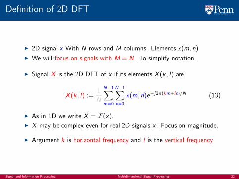
I 2D signal x With N rows and M columns. Elements x(m, n)
I We will focus on signals with M = N. To simplify notation.
I Signal X is the 2D DFT of x if its elements X (k , l) are
X (k, l) :=1
N
N−1∑m=0
N−1∑n=0
x(m, n)e−j2π(km+ln)/N (13)
I As in 1D we write X = F(x).
I X may be complex even for real 2D signals x . Focus on magnitude.
I Argument k is horizontal frequency and l is the vertical frequency
Signal and Information Processing Multidimensional Signal Processing 22
The 2D DFT and the (regular, 1D) DFT
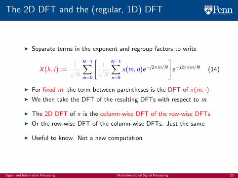
I Separate terms in the exponent and regroup factors to write
X (k , l) :=1√N
N−1∑m=0
[1√N
N−1∑n=0
x(m, n)e−j2πln/N
]e−j2πkm/N (14)
I For fixed m, the term between parentheses is the DFT of x(m, ·)I We then take the DFT of the resulting DFTs with respect to m
I The 2D DFT of x is the column-wise DFT of the row-wise DFTs
I Or the row-wise DFT of the column-wise DFTs. Just the same
I Useful to know. Not a new computation
Signal and Information Processing Multidimensional Signal Processing 23
Discrete complex exponentials
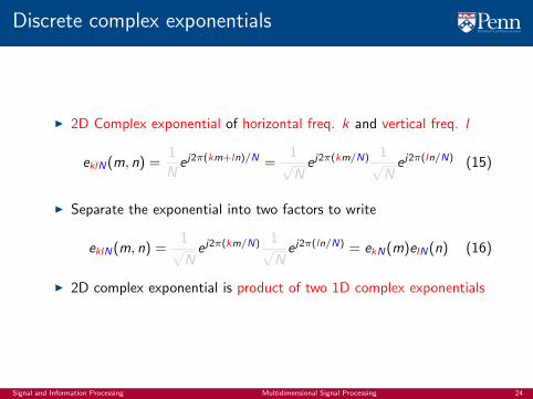
I 2D Complex exponential of horizontal freq. k and vertical freq. l
eklN(m, n) =1
Ne j2π(km+ln)/N =
1√Ne j2π(km/N) 1√
Ne j2π(ln/N) (15)
I Separate the exponential into two factors to write
eklN(m, n) =1√Ne j2π(km/N) 1√
Ne j2π(ln/N) = ekN(m)elN(n) (16)
I 2D complex exponential is product of two 1D complex exponentials
Signal and Information Processing Multidimensional Signal Processing 24
What 2D complex exponentials look like
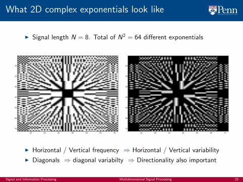
I Signal length N = 8. Total of N2 = 64 different exponentials
10 20 30 40 50 60 70
10
20
30
40
50
60
70
10 20 30 40 50 60 70
10
20
30
40
50
60
70
I Horizontal / Vertical frequency ⇒ Horizontal / Vertical variability
I Diagonals ⇒ diagonal variabilty ⇒ Directionality also important
Signal and Information Processing Multidimensional Signal Processing 25
What 2D complex exponentials look like
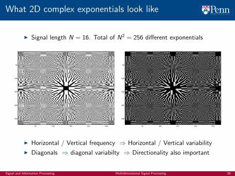
I Signal length N = 16. Total of N2 = 256 different exponentials
50 100 150 200 250
50
100
150
200
250
50 100 150 200 250
50
100
150
200
250
I Horizontal / Vertical frequency ⇒ Horizontal / Vertical variability
I Diagonals ⇒ diagonal variabilty ⇒ Directionality also important
Signal and Information Processing Multidimensional Signal Processing 26
DFT elements as inner products
I Rewrite 2D DFT using definition of 2D complex exponential
X (k, l) =N−1∑m=0
N−1∑n=0
x(m, n)e(−k)(−l)N(m, n) =N−1∑m=0
N−1∑n=0
x(m, n)e∗klN(m, n)
(17)
I From definition of inner product we have ⇒ X (k, l) = 〈x , eklN〉
I DFT element X (k , l) ⇒ Inner product of x(m, n) with ekl,N(m, n)
I How much x is an oscillation of horizontal freq. k vertical freq. l
I 2D DFT contains information on rate of change as the 1D DFT
⇒ But also on the direction of change
Signal and Information Processing Multidimensional Signal Processing 27

2D DFT of an image
I This is 256× 256 image. We rarely do DFTs of full images
⇒ Separate in 256 patches, each with 16× 16 pixels
Signal and Information Processing Multidimensional Signal Processing 28
A patch and its 2D DFT
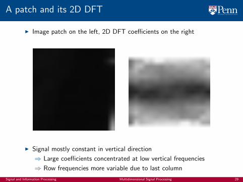
I Image patch on the left, 2D DFT coefficients on the right
I Signal mostly constant in vertical direction
⇒ Large coefficients concentrated at low vertical frequencies
⇒ Row frequencies more variable due to last column
Signal and Information Processing Multidimensional Signal Processing 29
A patch and its 2D DFT
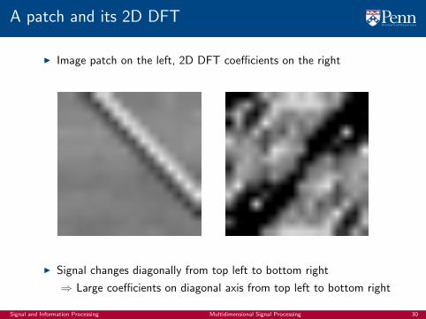
I Image patch on the left, 2D DFT coefficients on the right
I Signal changes diagonally from top left to bottom right
⇒ Large coefficients on diagonal axis from top left to bottom right
Signal and Information Processing Multidimensional Signal Processing 30
A patch and its 2D DFT
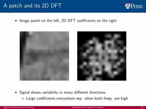
I Image patch on the left, 2D DFT coefficients on the right
I Signal shows variability in many different directions
⇒ Large coefficients everywhere esp. when both freqs. are high
Signal and Information Processing Multidimensional Signal Processing 31
The DFT and variability
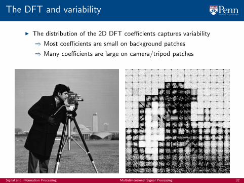
I The distribution of the 2D DFT coefficients captures variability
⇒ Most coefficients are small on background patches
⇒ Many coefficients are large on camera/tripod patches
Signal and Information Processing Multidimensional Signal Processing 32
Periodicity of complex exponentials
I We know that there are only N distinct complex exponentials
I Thus, there are only N2 distinct 2D complex exponentials
⇒ Horizontal frequencies k and k + N are equivalent
⇒ Vertical frequencies l and l + N are equivalent
I Canonical sets [0,N − 1]× [0,N − 1] and [−N/2,N/2]× [−N/2,N/2]
I 1D complex exponentials are conjugate symmetric. Thus
e(−k)(−l)N ≡ e∗klN (18)
I Flipping sign of both freqs ≡ Conjugation of complex exponential
Signal and Information Processing Multidimensional Signal Processing 33
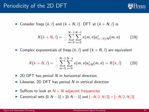
Periodicity of the 2D DFT
I Consider freqs (k , l) and (k + N, l). DFT at (k + N, l) is
X (k + N, l) =1
N
N−1∑m=0
N−1∑n=0
x(m, n)e∗(k+N)lN(m, n) (19)
I Complex exponentials of freqs.(k , l) and (k + N, l) are equivalent
X (k + N, l) =1
N
N−1∑m=0
N−1∑n=0
x(m, n)e∗klN(m, n) = X (k, l) (20)
I 2D DFT has period N in horizontal direction.
I Likewise, 2D DFT has period N in vertical direction
I Suffices to look at N × N adjacent frequencies
I Canonical sets [0,N − 1]× [0,N − 1] and [−N/2,N/2]× [−N/2,N/2]
Signal and Information Processing Multidimensional Signal Processing 34
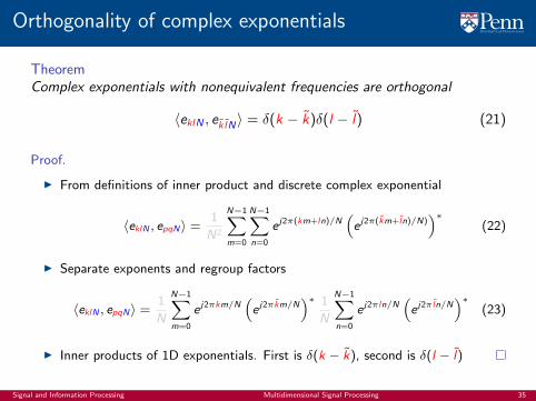
Orthogonality of complex exponentials
TheoremComplex exponentials with nonequivalent frequencies are orthogonal
〈eklN , ek lN〉 = δ(k − k)δ(l − l) (21)
Proof.
I From definitions of inner product and discrete complex exponential
〈eklN , epqN〉 =1
N2
N−1∑m=0
N−1∑n=0
e j2π(km+ln)/N(e j2π(km+ln)/N)
)∗(22)
I Separate exponents and regroup factors
〈eklN , epqN〉 =1
N
N−1∑m=0
e j2πkm/N(e j2πkm/N
)∗ 1
N
N−1∑n=0
e j2πln/N(e j2πln/N
)∗(23)
I Inner products of 1D exponentials. First is δ(k − k), second is δ(l − l)
Signal and Information Processing Multidimensional Signal Processing 35

Two dimensional (2D) iDFT
Signal representation
Images
Two dimensional discrete signals
Two dimensional (2D) discrete Fourier transform (DFT)
Two dimensional (2D) inverse (i) discrete Fourier transform (DFT)
Energy conservation (Parseval’s theorem)
Convolution in 2 dimensions
Applications
Discrete Cosine Transform
2D Discrete Cosine Transform
JPEG image compression
Signal and Information Processing Multidimensional Signal Processing 36
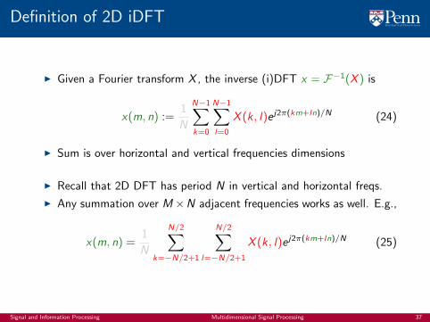
Definition of 2D iDFT
I Given a Fourier transform X , the inverse (i)DFT x = F−1(X ) is
x(m, n) :=1
N
N−1∑k=0
N−1∑l=0
X (k , l)e j2π(km+ln)/N (24)
I Sum is over horizontal and vertical frequencies dimensions
I Recall that 2D DFT has period N in vertical and horizontal freqs.
I Any summation over M ×N adjacent frequencies works as well. E.g.,
x(m, n) =1
N
N/2∑k=−N/2+1
N/2∑l=−N/2+1
X (k , l)e j2π(km+ln)/N (25)
Signal and Information Processing Multidimensional Signal Processing 37
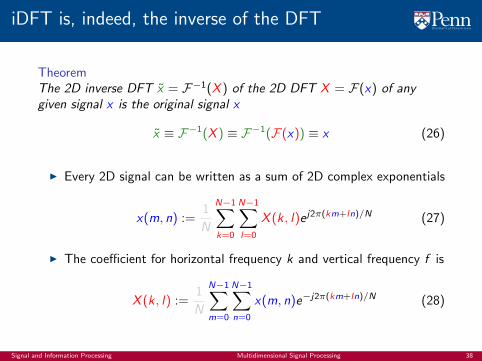
iDFT is, indeed, the inverse of the DFT
TheoremThe 2D inverse DFT x = F−1(X ) of the 2D DFT X = F(x) of anygiven signal x is the original signal x
x ≡ F−1(X ) ≡ F−1(F(x)) ≡ x (26)
I Every 2D signal can be written as a sum of 2D complex exponentials
x(m, n) :=1
N
N−1∑k=0
N−1∑l=0
X (k , l)e j2π(km+ln)/N (27)
I The coefficient for horizontal frequency k and vertical frequency f is
X (k, l) :=1
N
N−1∑m=0
N−1∑n=0
x(m, n)e−j2π(km+ln)/N (28)
Signal and Information Processing Multidimensional Signal Processing 38
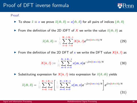
Proof of DFT inverse formula
Proof.
I To show x ≡ x we prove x(m, n) = x(m, n) for all pairs of indices (m, n)
I From the definition of the 2D iDFT of X we write the value x(m, n) as
x(m, n) =1
N
N−1∑k=0
N−1∑l=0
X (k, l)e j2π(km+l n)/N (29)
I From the definition of the 2D DFT of x we write the DFT value X (k, l) as
X (k, l) :=1
N
N−1∑m=0
N−1∑n=0
x(m, n)e−j2π(km+ln)/N (30)
I Substituting expression for X (k, l) into expression for x(n, m) yields
x(m, n) =1
N
N−1∑k=0
N−1∑l=0
[1
N
N−1∑m=0
N−1∑n=0
x(m, n)e−j2π(km+ln)/N
]e j2π(km+l n)/N
(31)
Signal and Information Processing Multidimensional Signal Processing 39
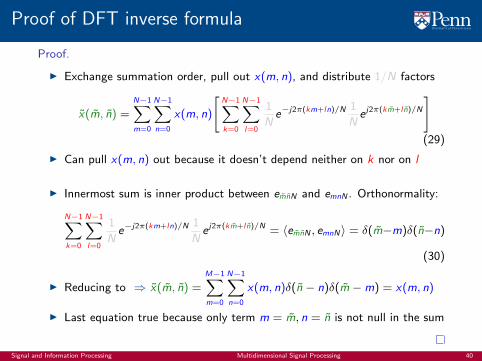
Proof of DFT inverse formula
Proof.
I Exchange summation order, pull out x(m, n), and distribute 1/N factors
x(m, n) =N−1∑m=0
N−1∑n=0
x(m, n)
[N−1∑k=0
N−1∑l=0
1
Ne−j2π(km+ln)/N 1
Ne j2π(km+l n)/N
](29)
I Can pull x(m, n) out because it doesn’t depend neither on k nor on l
I Innermost sum is inner product between emnN and emnN . Orthonormality:
N−1∑k=0
N−1∑l=0
1
Ne−j2π(km+ln)/N 1
Ne j2π(km+l n)/N = 〈emnN , emnN〉 = δ(m−m)δ(n−n)
(30)
I Reducing to ⇒ x(m, n) =M−1∑m=0
N−1∑n=0
x(m, n)δ(n − n)δ(m −m) = x(m, n)
I Last equation true because only term m = m, n = n is not null in the sum
Signal and Information Processing Multidimensional Signal Processing 40
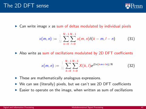
The 2D DFT sense
I Can write image x as sum of deltas modulated by individual pixels
x(m, n) :=1
N
N−1∑k=0
N−1∑l=0
x(m, n)δ(k −m, l − n) (31)
I Also write as sum of oscillations modulated by 2D DFT coefficients
x(m, n) :=1
N
N−1∑k=0
N−1∑l=0
X (k , l)e j2π(km+ln)/N (32)
I These are mathematically analogous expressions.
I We can see (literally) pixels, but we can’t see 2D DFT coefficients
I Easier to operate on the image, when written as sum of oscillations
Signal and Information Processing Multidimensional Signal Processing 41
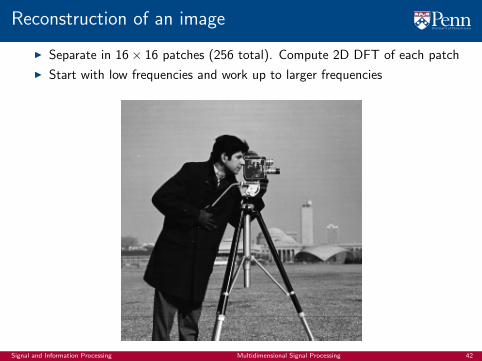
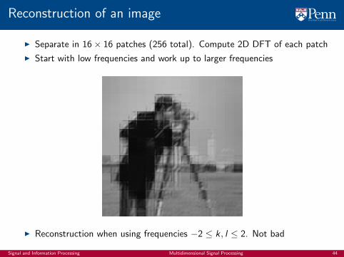
Reconstruction of an image
I Separate in 16× 16 patches (256 total). Compute 2D DFT of each patch
I Start with low frequencies and work up to larger frequencies
ISignal and Information Processing Multidimensional Signal Processing 42

Reconstruction of an image
I Separate in 16× 16 patches (256 total). Compute 2D DFT of each patch
I Start with low frequencies and work up to larger frequencies
I Reconstruction when using frequencies −1 ≤ k , l ≤ 1. Not too good
Signal and Information Processing Multidimensional Signal Processing 43
Reconstruction of an image
I Separate in 16× 16 patches (256 total). Compute 2D DFT of each patch
I Start with low frequencies and work up to larger frequencies
I Reconstruction when using frequencies −2 ≤ k , l ≤ 2. Not bad
Signal and Information Processing Multidimensional Signal Processing 44

Reconstruction of an image
I Separate in 16× 16 patches (256 total). Compute 2D DFT of each patch
I Start with low frequencies and work up to larger frequencies
I Using frequencies −4 ≤ k , l ≤ 4. Quite good, except for border effect
Signal and Information Processing Multidimensional Signal Processing 45

Reconstruction of an image
I Separate in 16× 16 patches (256 total). Compute 2D DFT of each patch
I Start with low frequencies and work up to larger frequencies
I Freqs. −7 ≤ k, l ≤ 7. Border effect still present. Will solve later (DCT)
Signal and Information Processing Multidimensional Signal Processing 46
Energy conservation (Parseval’s theorem)
Signal representation
Images
Two dimensional discrete signals
Two dimensional (2D) discrete Fourier transform (DFT)
Two dimensional (2D) inverse (i) discrete Fourier transform (DFT)
Energy conservation (Parseval’s theorem)
Convolution in 2 dimensions
Applications
Discrete Cosine Transform
2D Discrete Cosine Transform
JPEG image compression
Signal and Information Processing Multidimensional Signal Processing 47
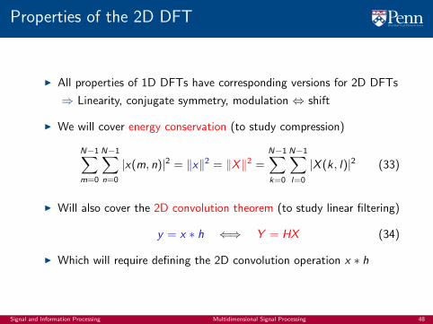
Properties of the 2D DFT
I All properties of 1D DFTs have corresponding versions for 2D DFTs
⇒ Linearity, conjugate symmetry, modulation ⇔ shift
I We will cover energy conservation (to study compression)
N−1∑m=0
N−1∑n=0
|x(m, n)|2 = ‖x‖2 = ‖X‖2 =N−1∑k=0
N−1∑l=0
|X (k, l)|2 (33)
I Will also cover the 2D convolution theorem (to study linear filtering)
y = x ∗ h ⇐⇒ Y = HX (34)
I Which will require defining the 2D convolution operation x ∗ h
Signal and Information Processing Multidimensional Signal Processing 48
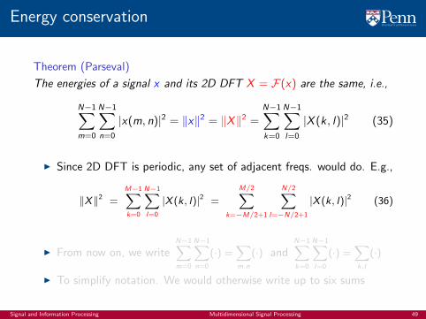
Energy conservation
Theorem (Parseval)
The energies of a signal x and its 2D DFT X = F(x) are the same, i.e.,
N−1∑m=0
N−1∑n=0
|x(m, n)|2 = ‖x‖2 = ‖X‖2 =N−1∑k=0
N−1∑l=0
|X (k, l)|2 (35)
I Since 2D DFT is periodic, any set of adjacent freqs. would do. E.g.,
‖X‖2 =M−1∑k=0
N−1∑l=0
|X (k, l)|2 =
M/2∑k=−M/2+1
N/2∑l=−N/2+1
|X (k, l)|2 (36)
I From now on, we writeN−1∑m=0
N−1∑n=0
(·) =∑m,n
(·) andN−1∑k=0
N−1∑l=0
(·) =∑k,l
(·)
I To simplify notation. We would otherwise write up to six sums
Signal and Information Processing Multidimensional Signal Processing 49
Proof of Parseval’s Theorem
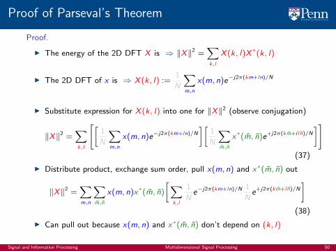
Proof.
I The energy of the 2D DFT X is ⇒ ‖X‖2 =∑k,l
X (k, l)X ∗(k, l)
I The 2D DFT of x is ⇒ X (k, l) :=1
N
∑m,n
x(m, n)e−j2π(km+ln)/N
I Substitute expression for X (k, l) into one for ‖X‖2 (observe conjugation)
‖X‖2 =∑k,l
[[1
N
∑m,n
x(m, n)e−j2π(km+ln)/N
][1
N
∑m,n
x∗(m, n)e+j2π(km+i l n)/N
]](37)
I Distribute product, exchange sum order, pull x(m, n) and x∗(m, n) out
‖X‖2 =∑m,n
∑m,n
x(m, n)x∗(m, n)
[∑k,l
1
Ne−j2π(km+ln)/N 1
Ne+j2π(km+l n)/N
](38)
I Can pull out because x(m, n) and x∗(m, n) don’t depend on (k, l)
Signal and Information Processing Multidimensional Signal Processing 50
Proof of Parseval’s Theorem
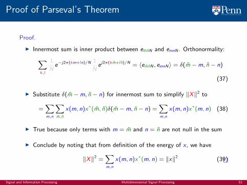
Proof.
I Innermost sum is inner product between emnN and emnN . Orthonormality:∑k,l
1
Ne−j2π(km+ln)/N 1
Ne j2π(km+l n)/N = 〈emnN , emnN〉 = δ(m −m, n − n)
(37)
I Substitute δ(m −m, n − n) for innermost sum to simplify ‖X‖2 to
=∑m,n
∑m,n
x(m, n)x∗(m, n)δ(m −m, n − n) =∑m,n
x(m, n)x∗(m, n) (38)
I True because only terms with m = m and n = n are not null in the sum
I Conclude by noting that from definition of the energy of x , we have
‖X‖2 =∑m,n
x(m, n)x∗(m, n) = ‖x‖2 (39)
Signal and Information Processing Multidimensional Signal Processing 51

Reconstruction of an image
I Separate in 16× 16 patches (256 total). Compute 2D DFT of each patch
I Start with low frequencies and work up to larger frequencies
I Energy of approximation error ≡ Energy of 2D DFT coefficients dropped
Signal and Information Processing Multidimensional Signal Processing 52

Reconstruction of an image
I Separate in 16× 16 patches (256 total). Compute 2D DFT of each patch
I Start with low frequencies and work up to larger frequencies
I Energy of reconstruction error ⇒ 32% of image’s energy (4 coefficients)
Signal and Information Processing Multidimensional Signal Processing 53

Reconstruction of an image
I Separate in 16× 16 patches (256 total). Compute 2D DFT of each patch
I Start with low frequencies and work up to larger frequencies
I Energy of reconstruction error ⇒ 9% of image’s energy (16 coefficients)
Signal and Information Processing Multidimensional Signal Processing 54
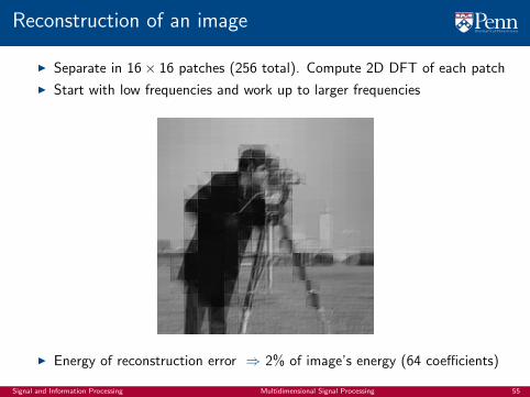
Reconstruction of an image
I Separate in 16× 16 patches (256 total). Compute 2D DFT of each patch
I Start with low frequencies and work up to larger frequencies
I Energy of reconstruction error ⇒ 2% of image’s energy (64 coefficients)
Signal and Information Processing Multidimensional Signal Processing 55
Convolution in 2 dimensions
Signal representation
Images
Two dimensional discrete signals
Two dimensional (2D) discrete Fourier transform (DFT)
Two dimensional (2D) inverse (i) discrete Fourier transform (DFT)
Energy conservation (Parseval’s theorem)
Convolution in 2 dimensions
Applications
Discrete Cosine Transform
2D Discrete Cosine Transform
JPEG image compression
Signal and Information Processing Multidimensional Signal Processing 56
2D Convolution
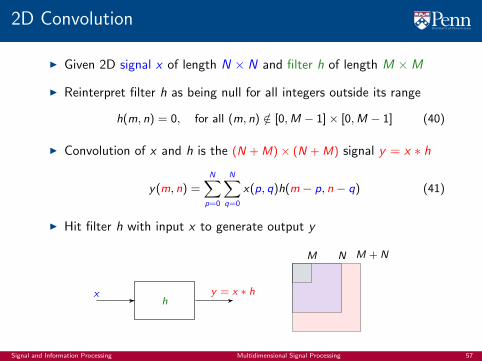
I Given 2D signal x of length N × N and filter h of length M ×M
I Reinterpret filter h as being null for all integers outside its range
h(m, n) = 0, for all (m, n) /∈ [0,M − 1]× [0,M − 1] (40)
I Convolution of x and h is the (N + M)× (N + M) signal y = x ∗ h
y(m, n) =N∑
p=0
N∑q=0
x(p, q)h(m − p, n − q) (41)
I Hit filter h with input x to generate output y
xh
y = x ∗ h
M + NNM
Signal and Information Processing Multidimensional Signal Processing 57
Padded signals
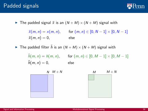
I The padded signal x is an (N + M)× (N + M) signal with
x(m, n) = x(m, n), for (m, n) ∈ [0,N − 1]× [0,N − 1]
x(m, n) = 0, else
I The padded filter h is an (N + M)× (N + M) signal with
h(m, n) = h(m, n), for (m, n) ∈ [0,M − 1]× [0,M − 1]
h(m, n) = 0, else
M + NN M + NM
Signal and Information Processing Multidimensional Signal Processing 58
2D convolution theorem
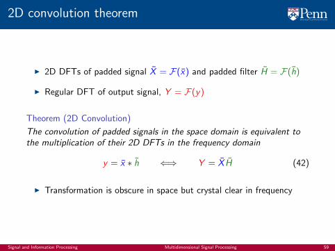
I 2D DFTs of padded signal X = F(x) and padded filter H = F(h)
I Regular DFT of output signal, Y = F(y)
Theorem (2D Convolution)
The convolution of padded signals in the space domain is equivalent tothe multiplication of their 2D DFTs in the frequency domain
y = x ∗ h ⇐⇒ Y = X H (42)
I Transformation is obscure in space but crystal clear in frequency
Signal and Information Processing Multidimensional Signal Processing 59
Design in frequency, implement in space
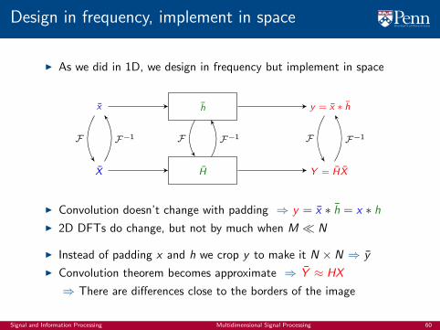
I As we did in 1D, we design in frequency but implement in space
x h y = x ∗ h
X H Y = HX
F F−1 F F−1 F F−1
I Convolution doesn’t change with padding ⇒ y = x ∗ h = x ∗ hI 2D DFTs do change, but not by much when M � N
I Instead of padding x and h we crop y to make it N × N ⇒ y
I Convolution theorem becomes approximate ⇒ Y ≈ HX
⇒ There are differences close to the borders of the image
Signal and Information Processing Multidimensional Signal Processing 60
Applications
Signal representation
Images
Two dimensional discrete signals
Two dimensional (2D) discrete Fourier transform (DFT)
Two dimensional (2D) inverse (i) discrete Fourier transform (DFT)
Energy conservation (Parseval’s theorem)
Convolution in 2 dimensions
Applications
Discrete Cosine Transform
2D Discrete Cosine Transform
JPEG image compression
Signal and Information Processing Multidimensional Signal Processing 61
Averaging Filter
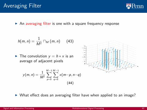
I An averaging filter is one with a square frequency response
h(m, n) =1
M2uM (m, n) (43)
I The convolution y = h ∗ x is anaverage of adjacent pixels
y(m, n) =1
M2
M−1∑p=0
M−1∑q=0
x(m−p, n−q)
(44)
I What effect does an averaging filter have when applied to an image?
Signal and Information Processing Multidimensional Signal Processing 62

Image Blurring
I Averaging neighboring pixels has the effect of blurring the image
I What is the counterpart of blurring in the frequency domain?
Signal and Information Processing Multidimensional Signal Processing 63
Average Filter in frequency domain
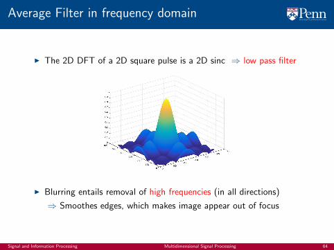
I The 2D DFT of a 2D square pulse is a 2D sinc ⇒ low pass filter
I Blurring entails removal of high frequencies (in all directions)
⇒ Smoothes edges, which makes image appear out of focus
Signal and Information Processing Multidimensional Signal Processing 64
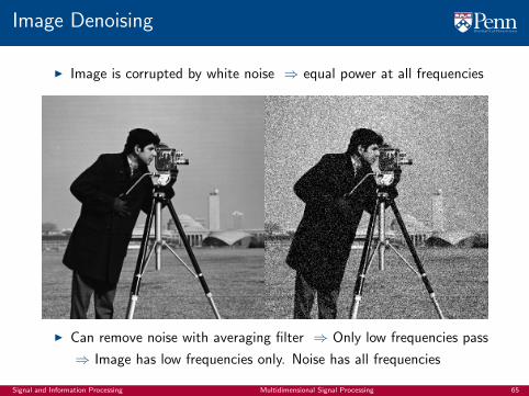
Image Denoising
I Image is corrupted by white noise ⇒ equal power at all frequencies
I Can remove noise with averaging filter ⇒ Only low frequencies pass
⇒ Image has low frequencies only. Noise has all frequencies
Signal and Information Processing Multidimensional Signal Processing 65
Gaussian filter
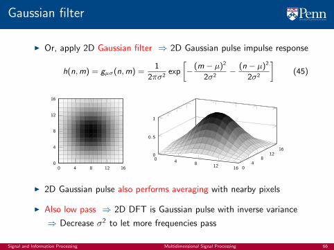
I Or, apply 2D Gaussian filter ⇒ 2D Gaussian pulse impulse response
h(n,m) = gµσ(n,m) =1
2πσ2exp
[− (m − µ)2
2σ2− (n − µ)2
2σ2
](45)
0 4 8 12 160
4
8
12
16
0 4 812 16 0
48
1216
0
0.5
1
I 2D Gaussian pulse also performs averaging with nearby pixels
I Also low pass ⇒ 2D DFT is Gaussian pulse with inverse variance
⇒ Decrease σ2 to let more frequencies pass
Signal and Information Processing Multidimensional Signal Processing 66
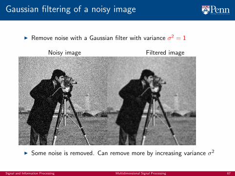
Gaussian filtering of a noisy image
I Remove noise with a Gaussian filter with variance σ2 = 1
Noisy image Filtered image
I Some noise is removed. Can remove more by increasing variance σ2
Signal and Information Processing Multidimensional Signal Processing 67
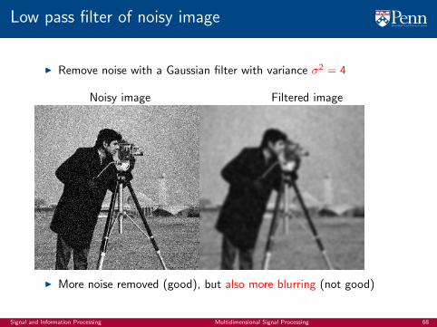
Low pass filter of noisy image
I Remove noise with a Gaussian filter with variance σ2 = 4
Noisy image Filtered image
I More noise removed (good), but also more blurring (not good)
Signal and Information Processing Multidimensional Signal Processing 68
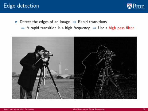
Edge detection
I Detect the edges of an image ⇒ Rapid transitions
⇒ A rapid transition is a high frequency ⇒ Use a high pass filter
Signal and Information Processing Multidimensional Signal Processing 69
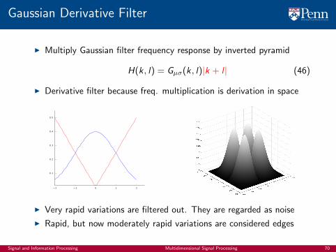
Gaussian Derivative Filter
I Multiply Gaussian filter frequency response by inverted pyramid
H(k , l) = Gµσ(k , l)|k + l | (46)
I Derivative filter because freq. multiplication is derivation in space
−2 −1 0 1 2
0.1
0.2
0.3
0.4
0.5
I Very rapid variations are filtered out. They are regarded as noise
I Rapid, but now moderately rapid variations are considered edges
Signal and Information Processing Multidimensional Signal Processing 70
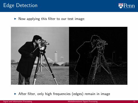
Edge Detection
I Now applying this filter to our test image:
I After filter, only high frequencies (edges) remain in image
Signal and Information Processing Multidimensional Signal Processing 71
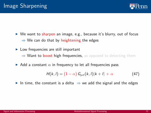
Image Sharpening
I We want to sharpen an image, e.g., because it’s blurry, out of focus
⇒ We can do that by heightening the edges
I Low frequencies are still important
⇒ Want to boost high frequencies, as opposed to detecting them
I Add a constant α in frequency to let all frequencies pass
H(k, l) = (1− α)Gµσ(k , l)|k + l | + α (47)
I In time, the constant is a delta ⇒ we add the signal and the edges
Signal and Information Processing Multidimensional Signal Processing 72

Image Sharpening
I Increasing sharpening makes borders more defined
Signal and Information Processing Multidimensional Signal Processing 73
Discrete Cosine Transform
Signal representation
Images
Two dimensional discrete signals
Two dimensional (2D) discrete Fourier transform (DFT)
Two dimensional (2D) inverse (i) discrete Fourier transform (DFT)
Energy conservation (Parseval’s theorem)
Convolution in 2 dimensions
Applications
Discrete Cosine Transform
2D Discrete Cosine Transform
JPEG image compression
Signal and Information Processing Multidimensional Signal Processing 74
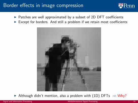
Border effects in image compression
I Patches are well approximated by a subset of 2D DFT coefficientsI Except for borders. And still a problem if we retain most coefficients
I Although didn’t mention, also a problem with (1D) DFTs ⇒ Why?
Signal and Information Processing Multidimensional Signal Processing 75
The DFT and the iDFT
I Start with real signal x : [0,N − 1]→ R. The DFT of signal x is
X (k) :=1√N
N−1∑n=0
x(n)e−j2πkn/N (48)
I We can recover x with the iDFT transformation defined by
x(n) :=1√N
N−1∑k=0
X (k)e j2πkn/N (49)
I We know that x(n) = x(n) for n ∈ [0,N − 1] (inverse transform)
I But the iDFT is defined for all n
I Signal x is periodic with period N because exponentials e j2πkn/N are
⇒ We say that iDFT signal x is a periodic extension of original x
Signal and Information Processing Multidimensional Signal Processing 76
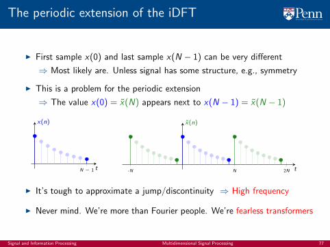
The periodic extension of the iDFT
I First sample x(0) and last sample x(N − 1) can be very different
⇒ Most likely are. Unless signal has some structure, e.g., symmetry
I This is a problem for the periodic extension
⇒ The value x(0) = x(N) appears next to x(N − 1) = x(N − 1)
N − 1 t
x(n)
-N N 2N t
x(n)
I It’s tough to approximate a jump/discontinuity ⇒ High frequency
I Never mind. We’re more than Fourier people. We’re fearless transformers
Signal and Information Processing Multidimensional Signal Processing 77
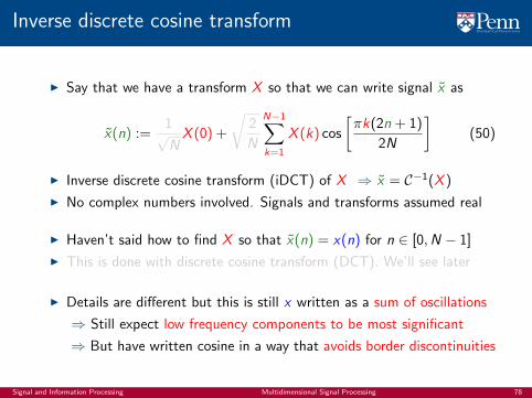
Inverse discrete cosine transform
I Say that we have a transform X so that we can write signal x as
x(n) :=1√NX (0) +
√2
N
N−1∑k=1
X (k) cos
[πk(2n + 1)
2N
](50)
I Inverse discrete cosine transform (iDCT) of X ⇒ x = C−1(X )
I No complex numbers involved. Signals and transforms assumed real
I Haven’t said how to find X so that x(n) = x(n) for n ∈ [0,N − 1]
I This is done with discrete cosine transform (DCT). We’ll see later
I Details are different but this is still x written as a sum of oscillations
⇒ Still expect low frequency components to be most significant
⇒ But have written cosine in a way that avoids border discontinuities
Signal and Information Processing Multidimensional Signal Processing 78

The iDCT is an even function
I Put a mirror at N − 1/2 and compare samples in each direction
I The sample at n = N − 1 can be written in terms of iDCT as
x(N − 1) :=1√NX (0) +
√2
N
N−1∑k=1
X (k) cos
[πk(N − 1 + 1/2)
N
]
=1√NX (0) +
√2
N
N−1∑k=1
X (k) cos
[πk +
πk(−1/2)
N
]
I The sample at n = N can be written in terms of iDCT as
x(N ) :=1√NX (0) +
√2
N
N−1∑k=1
X (k) cos
[πk(N + 1/2)
N
]
=1√NX (0) +
√2
N
N−1∑k=1
X (k) cos
[πk +
πk(1/2)
N
]
I Since cosines are even, sign is irrelevant. Thus ⇒ x(N − 1) = x(N)
Signal and Information Processing Multidimensional Signal Processing 79

The iDCT is an even function
I Put a mirror at N − 1/2 and compare samples in each direction
I The sample at n = N − 2 can be written in terms of iDCT as
x(N − 2) :=1√NX (0) +
√2
N
N−1∑k=1
X (k) cos
[πk(N − 2 + 1/2)
N
]
=1√NX (0) +
√2
N
N−1∑k=1
X (k) cos
[πk +
πk(−3/2)
N
]
I The sample at n = N + 1 can be written in terms of iDCT as
x(N + 1) :=1√NX (0) +
√2
N
N−1∑k=1
X (k) cos
[πk(N + 1 + 1/2)
N
]
=1√NX (0) +
√2
N
N−1∑k=1
X (k) cos
[πk +
πk(3/2)
N
]
I Since cosines are even, sign is irrelevant. Thus ⇒ x(N − 2) = x(N + 1)
Signal and Information Processing Multidimensional Signal Processing 80
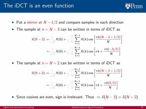
The iDCT is an even function
I Put a mirror at N − 1/2 and compare samples in each direction
I The sample at n = N − 3 can be written in terms of iDCT as
x(N − 3) :=1√NX (0) +
√2
N
N−1∑k=1
X (k) cos
[πk(N − 3 + 1/2)
N
]
=1√NX (0) +
√2
N
N−1∑k=1
X (k) cos
[πk +
πk(−5/2)
N
]
I The sample at n = N + 2 can be written in terms of iDCT as
x(N + 2) :=1√NX (0) +
√2
N
N−1∑k=1
X (k) cos
[πk(N + 2 + 1/2)
N
]
=1√NX (0) +
√2
N
N−1∑k=1
X (k) cos
[πk +
πk(5/2)
N
]
I Since cosines are even, sign is irrelevant. Thus ⇒ x(N − 3) = x(N + 2)
Signal and Information Processing Multidimensional Signal Processing 81

The iDCT is an even function
I Put a mirror at N − 1/2 and compare samples in each direction
I The sample at n = N − 4 can be written in terms of iDCT as
x(N − 4) :=1√NX (0) +
√2
N
N−1∑k=1
X (k) cos
[πk(N − 4 + 1/2)
N
]
=1√NX (0) +
√2
N
N−1∑k=1
X (k) cos
[πk +
πk(−7/2)
N
]
I The sample at n = N + 3 can be written in terms of iDCT as
x(N + 3) :=1√NX (0) +
√2
N
N−1∑k=1
X (k) cos
[πk(N + 3 + 1/2)
N
]
=1√NX (0) +
√2
N
N−1∑k=1
X (k) cos
[πk +
πk(7/2)
N
]
I Since cosines are even, sign is irrelevant. Thus ⇒ x(N − 4) = x(N + 3)
Signal and Information Processing Multidimensional Signal Processing 82
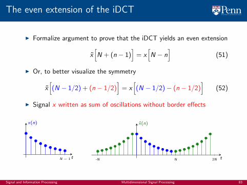
The even extension of the iDCT
I Formalize argument to prove that the iDCT yields an even extension
x[N + (n − 1)
]= x
[N − n
](51)
I Or, to better visualize the symmetry
x[(N − 1/2) + (n − 1/2)
]= x
[(N − 1/2)− (n − 1/2)
](52)
I Signal x written as sum of oscillations without border effects
N − 1 t
x(n)
-N N 2N t
x(n)
Signal and Information Processing Multidimensional Signal Processing 83
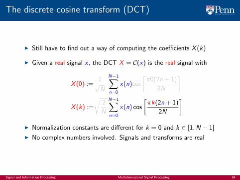
The discrete cosine transform (DCT)
I Still have to find out a way of computing the coefficients X (k)
I Given a real signal x , the DCT X = C(x) is the real signal with
X (0) :=1√N
N−1∑n=0
x(n)cos
[π0(2n + 1)
2N
]
X (k) :=
√2
N
N−1∑n=0
x(n) cos
[πk(2n + 1)
2N
]I Normalization constants are different for k = 0 and k ∈ [1,N − 1]
I No complex numbers involved. Signals and transforms are real
Signal and Information Processing Multidimensional Signal Processing 84
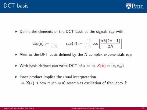
DCT basis
I Define the elements of the DCT basis as the signals ckN with
c0N(n) :=1√N
ckN(n) :=
√2
Ncos
[πk(2n + 1)
2N
]I Akin to the DFT basis defined by the N complex exponentials ekN
I With basis defined can write DCT of x as ⇒ X (k) = 〈x , ckN〉
I Inner product implies the usual interpretation
⇒ X(k) is how much x(n) resembles oscillation of frequency k
Signal and Information Processing Multidimensional Signal Processing 85
iDCT is the inverse of the DCT
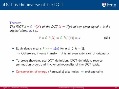
TheoremThe iDCT x = C−1(X ) of the DCT X = C(x) of any given signal x is theoriginal signal x , i.e.,
x ≡ C−1(X ) ≡ C−1(C(x)) ≡ x (53)
I Equivalence means x(n) = x(n) for n ∈ [0,N − 1].
⇒ Otherwise, inverse transform x is an even extension of original x
I To prove theorem, use DCT definition, iDCT definition, reversesummation order, and invoke orthogonality of the DCT basis.
I Conservation of energy (Parseval’s) also holds ⇒ orthogonality
Signal and Information Processing Multidimensional Signal Processing 86
2D Discrete Cosine Transform
Signal representation
Images
Two dimensional discrete signals
Two dimensional (2D) discrete Fourier transform (DFT)
Two dimensional (2D) inverse (i) discrete Fourier transform (DFT)
Energy conservation (Parseval’s theorem)
Convolution in 2 dimensions
Applications
Discrete Cosine Transform
2D Discrete Cosine Transform
JPEG image compression
Signal and Information Processing Multidimensional Signal Processing 87
Rewriting the 1D DCT
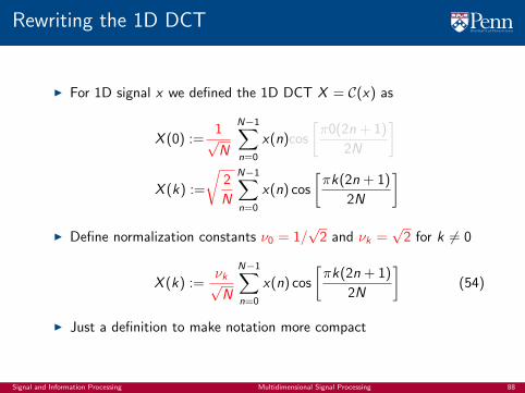
I For 1D signal x we defined the 1D DCT X = C(x) as
X (0) :=1√N
N−1∑n=0
x(n)cos
[π0(2n + 1)
2N
]
X (k) :=
√2
N
N−1∑n=0
x(n) cos
[πk(2n + 1)
2N
]I Define normalization constants ν0 = 1/
√2 and νk =
√2 for k 6= 0
X (k) :=νk√N
N−1∑n=0
x(n) cos
[πk(2n + 1)
2N
](54)
I Just a definition to make notation more compact
Signal and Information Processing Multidimensional Signal Processing 88
Two dimensional discrete cosine transform
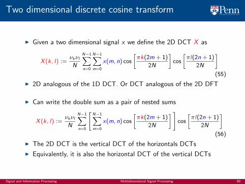
I Given a two dimensional signal x we define the 2D DCT X as
X (k, l) :=νkνlN
N−1∑n=0
N−1∑m=0
x(m, n) cos
[πk(2m + 1)
2N
]cos
[πl(2n + 1)
2N
](55)
I 2D analogous of the 1D DCT. Or DCT analogous of the 2D DFT
I Can write the double sum as a pair of nested sums
X (k, l) :=νkνlN
N−1∑n=0
[N−1∑m=0
x(m, n) cos
[πk(2m + 1)
2N
] ]cos
[πl(2n + 1)
2N
](56)
I The 2D DCT is the vertical DCT of the horizontals DCTs
I Equivalently, it is also the horizontal DCT of the vertical DCTs
Signal and Information Processing Multidimensional Signal Processing 89
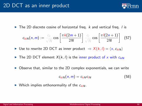
2D DCT as an inner product
I The 2D discrete cosine of horizontal freq. k and vertical freq. l is
cklN(n,m) :=ck√N
cos
[πk(2m + 1)
2N
]cl√N
cos
[πl(2n + 1)
2N
](57)
I Use to rewrite 2D DCT as inner product ⇒ X (k , l) = 〈x , cklN〉
I The 2D DCT element X (k , l) is the inner product of x with cklN
I Observe that, similar to the 2D complex exponentials, we can write
cklN(n,m) = ckNclN (58)
I Which implies orthonormality of the cklN .
Signal and Information Processing Multidimensional Signal Processing 90
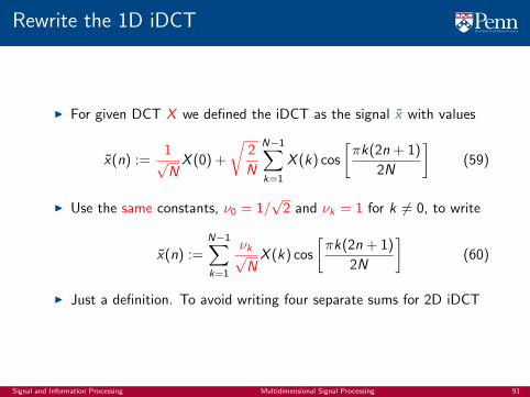
Rewrite the 1D iDCT
I For given DCT X we defined the iDCT as the signal x with values
x(n) :=1√NX (0) +
√2
N
N−1∑k=1
X (k) cos
[πk(2n + 1)
2N
](59)
I Use the same constants, ν0 = 1/√
2 and νk = 1 for k 6= 0, to write
x(n) :=N−1∑k=1
νk√NX (k) cos
[πk(2n + 1)
2N
](60)
I Just a definition. To avoid writing four separate sums for 2D iDCT
Signal and Information Processing Multidimensional Signal Processing 91
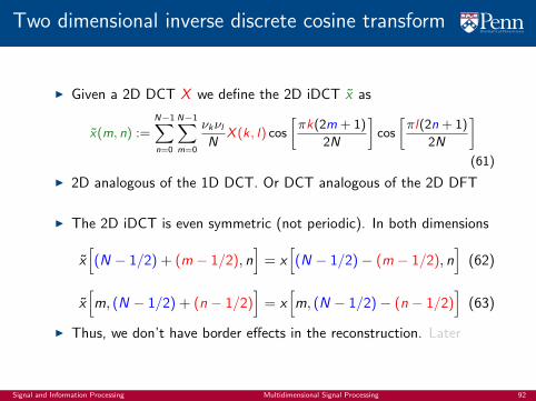
Two dimensional inverse discrete cosine transform
I Given a 2D DCT X we define the 2D iDCT x as
x(m, n) :=N−1∑n=0
N−1∑m=0
νkνlN
X (k, l) cos
[πk(2m + 1)
2N
]cos
[πl(2n + 1)
2N
](61)
I 2D analogous of the 1D DCT. Or DCT analogous of the 2D DFT
I The 2D iDCT is even symmetric (not periodic). In both dimensions
x[(N − 1/2) + (m − 1/2), n
]= x
[(N − 1/2)− (m − 1/2), n
](62)
x[m, (N − 1/2) + (n − 1/2)
]= x
[m, (N − 1/2)− (n − 1/2)
](63)
I Thus, we don’t have border effects in the reconstruction. Later
Signal and Information Processing Multidimensional Signal Processing 92

iDCT is the inverse of the DCT
TheoremThe iDCT x = C−1(X ) of the DCT X = C(x) of any given signal x is theoriginal signal x , i.e.,
x ≡ C−1(X ) ≡ C−1(C(x)) ≡ x (64)
I Equivalence means x(n) = x(n) for n ∈ [0,N − 1].
⇒ Otherwise, inverse transform x is an even extension of original x
I To prove theorem, use DCT definition, iDCT definition, reversesummation order, and invoke orthogonality of the DCT basis.
I Conservation of energy (Parseval’s) also holds ⇒ orthogonality
Signal and Information Processing Multidimensional Signal Processing 93
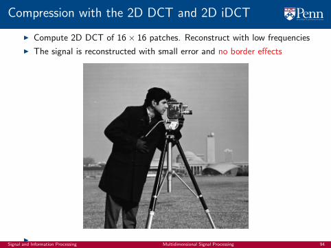
Compression with the 2D DCT and 2D iDCT
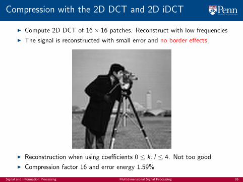
I Compute 2D DCT of 16× 16 patches. Reconstruct with low frequencies
I The signal is reconstructed with small error and no border effects
ISignal and Information Processing Multidimensional Signal Processing 94
Compression with the 2D DCT and 2D iDCT
I Compute 2D DCT of 16× 16 patches. Reconstruct with low frequencies
I The signal is reconstructed with small error and no border effects
I Reconstruction when using coefficients 0 ≤ k , l ≤ 4. Not too good
I Compression factor 16 and error energy 1.59%
Signal and Information Processing Multidimensional Signal Processing 95
Compression with the 2D DCT and 2D iDCT
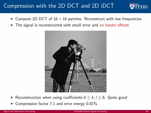
I Compute 2D DCT of 16× 16 patches. Reconstruct with low frequencies
I The signal is reconstructed with small error and no border effects
I Reconstruction when using coefficients 0 ≤ k , l ≤ 6. Quite good
I Compression factor 7.1 and error energy 0.81%
Signal and Information Processing Multidimensional Signal Processing 96

Compression with the 2D DCT and 2D iDCT
I Compute 2D DCT of 16× 16 patches. Reconstruct with low frequencies
I The signal is reconstructed with small error and no border effects
I Reconstruction when using coefficients 0 ≤ k , l ≤ 8. Excellent
I Compression factor 4 and error energy 0.46%
Signal and Information Processing Multidimensional Signal Processing 97

Compression with the 2D DCT and 2D iDCT
I Compute 2D DCT of 16× 16 patches. Reconstruct with low frequencies
I The signal is reconstructed with small error and no border effects
I Reconstruction when using coefficients 0 ≤ k , l ≤ 10. Flawless
I Compression factor 2.56 and error energy 0.26%
Signal and Information Processing Multidimensional Signal Processing 98

JPEG image compression
Signal representation
Images
Two dimensional discrete signals
Two dimensional (2D) discrete Fourier transform (DFT)
Two dimensional (2D) inverse (i) discrete Fourier transform (DFT)
Energy conservation (Parseval’s theorem)
Convolution in 2 dimensions
Applications
Discrete Cosine Transform
2D Discrete Cosine Transform
JPEG image compression
Signal and Information Processing Multidimensional Signal Processing 99
JPEG image compression
I Start with a color image ⇒ three color channels xR , xB , xG
⇒ Each pixel is represented by 8 bits
⇒ Values are integers in [0,255], or, equivalently [-127,128]
I Transform into luminance y and chrominance yR and yBI Eye more sensitive to luminance. Sample chrominances every 2 pixels
I Work with luminance and chrominance separately.
I Separate each channel in 8× 8 patches ⇒ 64 pixels per patch
I For each patch x , compute the corresponding DCT X
⇒ Keep coefficients associated with largest frequency components
I Low frequencies more important but high frequencies not irrelevant
⇒ Introduce importance quantization
Signal and Information Processing Multidimensional Signal Processing 100
Importance quantization
I For each frequency pair k , l , define the importance coefficient Q(k, l)
I Encode each DCT frequent component as
X (k , l) = round
(X (k , l)
Q(k , l)
)(65)
I If Q(k, l) ≈ 1 there is little change ⇒ X (k , l) ≈ X (k, l)
I If Q(k, l) is large we reduce the range of X (k , l)
I Numbers with smaller range can be encoded with less bits
⇒ Assign relatively small Q(k , l) to low frequencies
⇒ Assign relatively large Q(k , l) to high frequencies
Signal and Information Processing Multidimensional Signal Processing 101
Importance matrix
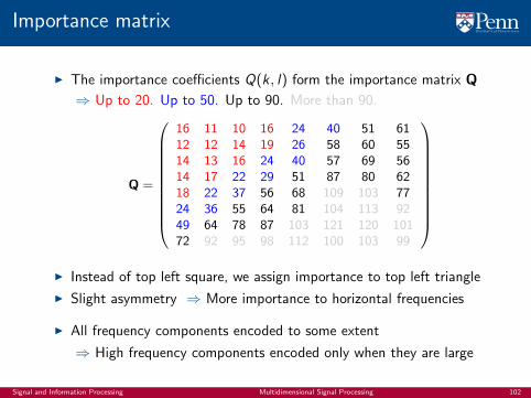
I The importance coefficients Q(k , l) form the importance matrix Q
⇒ Up to 20. Up to 50. Up to 90. More than 90.
Q =
16 11 10 16 24 40 51 6112 12 14 19 26 58 60 5514 13 16 24 40 57 69 5614 17 22 29 51 87 80 6218 22 37 56 68 109 103 7724 36 55 64 81 104 113 9249 64 78 87 103 121 120 10172 92 95 98 112 100 103 99
I Instead of top left square, we assign importance to top left triangle
I Slight asymmetry ⇒ More importance to horizontal frequencies
I All frequency components encoded to some extent
⇒ High frequency components encoded only when they are large
Signal and Information Processing Multidimensional Signal Processing 102