Embed Size (px)
DESCRIPTION
Book by Duistermaat J.J. and Kolk J.A.C.
Citation preview
CAMBRIDGE STUDIES INADVANCED MATHEMATICS 86
EDITORIAL BOARDB. BOLLOBÁS, W. FULTON, A. KATOK, F. KIRWAN,P. SARNAK, B. SIMON
MULTIDIMENSIONAL REALANALYSIS I:
DIFFERENTIATION
Already published; for full details see http://publishing.cambridge.org/stm /mathematics/csam/
11 J.L. Alperin Local representation theory
12 P. Koosis The logarithmic integral I13 A. Pietsch Eigenvalues and s-numbers14 S.J. Patterson An introduction to the theory of the Riemann zeta-function15 H.J. Baues Algebraic homotopy
16 V.S. Varadarajan Introduction to harmonic analysis on semisimple Lie groups17 W. Dicks & M. Dunwoody Groups acting on graphs18 L.J. Corwin & F.P. Greenleaf Representations of nilpotent Lie groups and their applications
19 R. Fritsch & R. Piccinini Cellular structures in topology20 H. Klingen Introductory lectures on Siegel modular forms21 P. Koosis The logarithmic integral II
22 M.J. Collins Representations and characters of finite groups24 H. Kunita Stochastic flows and stochastic differential equations25 P. Wojtaszczyk Banach spaces for analysts
26 J.E. Gilbert & M.A.M. Murray Clifford algebras and Dirac operators in harmonic analysis27 A. Frohlich & M.J. Taylor Algebraic number theory28 K. Goebel & W.A. Kirk Topics in metric fixed point theory29 J.E. Humphreys Reflection groups and Coxeter groups
30 D.J. Benson Representations and cohomology I31 D.J. Benson Representations and cohomology II32 C. Allday & V. Puppe Cohomological methods in transformation groups
33 C. Soulé et al Lectures on Arakelov geometry34 A. Ambrosetti & G. Prodi A primer of nonlinear analysis35 J. Palis & F. Takens Hyperbolicity, stability and chaos at homoclinic bifurcations
37 Y. Meyer Wavelets and operators I38 C. Weibel An introduction to homological algebra39 W. Bruns & J. Herzog Cohen-Macaulay rings
40 V. Snaith Explicit Brauer induction41 G. Laumon Cohomology of Drinfield modular varieties I42 E.B. Davies Spectral theory and differential operators
43 J. Diestel, H. Jarchow & A. Tonge Absolutely summing operators44 P. Mattila Geometry of sets and measures in euclidean spaces45 R. Pinsky Positive harmonic functions and diffusion46 G. Tenenbaum Introduction to analytic and probabilistic number theory
47 C. Peskine An algebraic introduction to complex projective geometry I48 Y. Meyer & R. Coifman Wavelets and operators II49 R. Stanley Enumerative combinatorics I
50 I. Porteous Clifford algebras and the classical groups51 M. Audin Spinning tops52 V. Jurdjevic Geometric control theory
53 H. Voelklein Groups as Galois groups54 J. Le Potier Lectures on vector bundles55 D. Bump Automorphic forms
56 G. Laumon Cohomology of Drinfeld modular varieties II57 D.M. Clarke & B.A. Davey Natural dualities for the working algebraist59 P. Taylor Practical foundations of mathematics60 M. Brodmann & R. Sharp Local cohomology
61 J.D. Dixon, M.P.F. Du Sautoy, A. Mann & D. Segal Analytic pro-p groups, 2nd edition62 R. Stanley Enumerative combinatorics II64 J. Jost & X. Li-Jost Calculus of variations
68 Ken-iti Sato Lévy processes and infinitely divisible distributions71 R. Blei Analysis in integer and fractional dimensions72 F. Borceux & G. Janelidze Galois theories
73 B. Bollobás Random graphs74 R.M. Dudley Real analysis and probability75 T. Sheil-Small Complex polynomials
76 C. Voisin Hodge theory and complex algebraic geometry I77 C. Voisin Hodge theory and complex algebraic geometry II78 V. Paulsen Completely bounded maps and operator algebra
79 F. Gesztesy & H. Holden Soliton equations and their algebro-geometric solutions I80 F. Gesztesy & H. Holden Soliton equations and their algebro-geometric solutions II
MULTIDIMENSIONAL REALANALYSIS I:
DIFFERENTIATION
J.J. DUISTERMAATJ.A.C. KOLK
Utrecht University
Translated from Dutch by J. P. van Braam Houckgeest
cambridge university pressCambridge, New York, Melbourne, Madrid, Cape Town, Singapore, São Paulo
Cambridge University PressThe Edinburgh Building, Cambridge cb2 2ru, UK
First published in print format
isbn-13 978-0-521-55114-4
isbn-13 978-0-511-19558-7
© Cambridge University Press 2004
2004
Information on this title: www.cambridge.org/9780521551144
This publication is in copyright. Subject to statutory exception and to the provision ofrelevant collective licensing agreements, no reproduction of any part may take placewithout the written permission of Cambridge University Press.
isbn-10 0-511-19558-3
isbn-10 0-521-55114-5
Cambridge University Press has no responsibility for the persistence or accuracy of urlsfor external or third-party internet websites referred to in this publication, and does notguarantee that any content on such websites is, or will remain, accurate or appropriate.
Published in the United States of America by Cambridge University Press, New York
www.cambridge.org
hardback
eBook (NetLibrary)
eBook (NetLibrary)
hardback
To Saskia and Floortje
With Gratitude and Love

Contents
Volume IPreface . . . . . . . . . . . . . . . . . . . . . . . . . . . . . . . . . xiAcknowledgments . . . . . . . . . . . . . . . . . . . . . . . . . . . . xiiiIntroduction . . . . . . . . . . . . . . . . . . . . . . . . . . . . . . . xv
1 Continuity 11.1 Inner product and norm . . . . . . . . . . . . . . . . . . . . . . 11.2 Open and closed sets . . . . . . . . . . . . . . . . . . . . . . . 61.3 Limits and continuous mappings . . . . . . . . . . . . . . . . . 111.4 Composition of mappings . . . . . . . . . . . . . . . . . . . . . 171.5 Homeomorphisms . . . . . . . . . . . . . . . . . . . . . . . . . 191.6 Completeness . . . . . . . . . . . . . . . . . . . . . . . . . . . 201.7 Contractions . . . . . . . . . . . . . . . . . . . . . . . . . . . . 231.8 Compactness and uniform continuity . . . . . . . . . . . . . . . 241.9 Connectedness . . . . . . . . . . . . . . . . . . . . . . . . . . 33
2 Differentiation 372.1 Linear mappings . . . . . . . . . . . . . . . . . . . . . . . . . 372.2 Differentiable mappings . . . . . . . . . . . . . . . . . . . . . 422.3 Directional and partial derivatives . . . . . . . . . . . . . . . . 472.4 Chain rule . . . . . . . . . . . . . . . . . . . . . . . . . . . . . 512.5 Mean Value Theorem . . . . . . . . . . . . . . . . . . . . . . . 562.6 Gradient . . . . . . . . . . . . . . . . . . . . . . . . . . . . . . 582.7 Higher-order derivatives . . . . . . . . . . . . . . . . . . . . . 612.8 Taylor’s formula . . . . . . . . . . . . . . . . . . . . . . . . . . 662.9 Critical points . . . . . . . . . . . . . . . . . . . . . . . . . . . 702.10 Commuting limit operations . . . . . . . . . . . . . . . . . . . 76
3 Inverse Function and Implicit Function Theorems 873.1 Diffeomorphisms . . . . . . . . . . . . . . . . . . . . . . . . . 873.2 Inverse Function Theorems . . . . . . . . . . . . . . . . . . . . 893.3 Applications of Inverse Function Theorems . . . . . . . . . . . 943.4 Implicitly defined mappings . . . . . . . . . . . . . . . . . . . 963.5 Implicit Function Theorem . . . . . . . . . . . . . . . . . . . . 1003.6 Applications of the Implicit Function Theorem . . . . . . . . . 101
vii
viii Contents
3.7 Implicit and Inverse Function Theorems on C . . . . . . . . . . 105
4 Manifolds 1074.1 Introductory remarks . . . . . . . . . . . . . . . . . . . . . . . 1074.2 Manifolds . . . . . . . . . . . . . . . . . . . . . . . . . . . . . 1094.3 Immersion Theorem . . . . . . . . . . . . . . . . . . . . . . . . 1144.4 Examples of immersions . . . . . . . . . . . . . . . . . . . . . 1184.5 Submersion Theorem . . . . . . . . . . . . . . . . . . . . . . . 1204.6 Examples of submersions . . . . . . . . . . . . . . . . . . . . . 1244.7 Equivalent definitions of manifold . . . . . . . . . . . . . . . . 1264.8 Morse’s Lemma . . . . . . . . . . . . . . . . . . . . . . . . . . 128
5 Tangent Spaces 1335.1 Definition of tangent space . . . . . . . . . . . . . . . . . . . . 1335.2 Tangent mapping . . . . . . . . . . . . . . . . . . . . . . . . . 1375.3 Examples of tangent spaces . . . . . . . . . . . . . . . . . . . . 1375.4 Method of Lagrange multipliers . . . . . . . . . . . . . . . . . 1495.5 Applications of the method of multipliers . . . . . . . . . . . . 1515.6 Closer investigation of critical points . . . . . . . . . . . . . . . 1545.7 Gaussian curvature of surface . . . . . . . . . . . . . . . . . . . 1565.8 Curvature and torsion of curve in R3 . . . . . . . . . . . . . . . 1595.9 One-parameter groups and infinitesimal generators . . . . . . . 1625.10 Linear Lie groups and their Lie algebras . . . . . . . . . . . . . 1665.11 Transversality . . . . . . . . . . . . . . . . . . . . . . . . . . . 172
Exercises 175Review Exercises . . . . . . . . . . . . . . . . . . . . . . . . . . . . 175Exercises for Chapter 1 . . . . . . . . . . . . . . . . . . . . . . . . . 201Exercises for Chapter 2 . . . . . . . . . . . . . . . . . . . . . . . . . 217Exercises for Chapter 3 . . . . . . . . . . . . . . . . . . . . . . . . . 259Exercises for Chapter 4 . . . . . . . . . . . . . . . . . . . . . . . . . 293Exercises for Chapter 5 . . . . . . . . . . . . . . . . . . . . . . . . . 317
Notation . . . . . . . . . . . . . . . . . . . . . . . . . . . . . . . . . . . 411Index . . . . . . . . . . . . . . . . . . . . . . . . . . . . . . . . . . . . 412
Volume IIPreface . . . . . . . . . . . . . . . . . . . . . . . . . . . . . . . . . xiAcknowledgments . . . . . . . . . . . . . . . . . . . . . . . . . . . . xiiiIntroduction . . . . . . . . . . . . . . . . . . . . . . . . . . . . . . . xv
6 Integration 4236.1 Rectangles . . . . . . . . . . . . . . . . . . . . . . . . . . . . . 4236.2 Riemann integrability . . . . . . . . . . . . . . . . . . . . . . . 4256.3 Jordan measurability . . . . . . . . . . . . . . . . . . . . . . . 429
Contents ix
6.4 Successive integration . . . . . . . . . . . . . . . . . . . . . . . 4356.5 Examples of successive integration . . . . . . . . . . . . . . . . 4396.6 Change of Variables Theorem: formulation and examples . . . . 4446.7 Partitions of unity . . . . . . . . . . . . . . . . . . . . . . . . . 4526.8 Approximation of Riemann integrable functions . . . . . . . . . 4556.9 Proof of Change of Variables Theorem . . . . . . . . . . . . . . 4576.10 Absolute Riemann integrability . . . . . . . . . . . . . . . . . . 4616.11 Application of integration: Fourier transformation . . . . . . . . 4666.12 Dominated convergence . . . . . . . . . . . . . . . . . . . . . . 4716.13 Appendix: two other proofs of Change of Variables Theorem . . 477
7 Integration over Submanifolds 4877.1 Densities and integration with respect to density . . . . . . . . . 4877.2 Absolute Riemann integrability with respect to density . . . . . 4927.3 Euclidean d-dimensional density . . . . . . . . . . . . . . . . . 4957.4 Examples of Euclidean densities . . . . . . . . . . . . . . . . . 4987.5 Open sets at one side of their boundary . . . . . . . . . . . . . . 5117.6 Integration of a total derivative . . . . . . . . . . . . . . . . . . 5187.7 Generalizations of the preceding theorem . . . . . . . . . . . . 5227.8 Gauss’ Divergence Theorem . . . . . . . . . . . . . . . . . . . 5277.9 Applications of Gauss’ Divergence Theorem . . . . . . . . . . . 530
8 Oriented Integration 5378.1 Line integrals and properties of vector fields . . . . . . . . . . . 5378.2 Antidifferentiation . . . . . . . . . . . . . . . . . . . . . . . . 5468.3 Green’s and Cauchy’s Integral Theorems . . . . . . . . . . . . . 5518.4 Stokes’ Integral Theorem . . . . . . . . . . . . . . . . . . . . . 5578.5 Applications of Stokes’ Integral Theorem . . . . . . . . . . . . 5618.6 Apotheosis: differential forms and Stokes’ Theorem . . . . . . . 5678.7 Properties of differential forms . . . . . . . . . . . . . . . . . . 5768.8 Applications of differential forms . . . . . . . . . . . . . . . . . 5818.9 Homotopy Lemma . . . . . . . . . . . . . . . . . . . . . . . . 5858.10 Poincaré’s Lemma . . . . . . . . . . . . . . . . . . . . . . . . 5898.11 Degree of mapping . . . . . . . . . . . . . . . . . . . . . . . . 591
Exercises 599Exercises for Chapter 6 . . . . . . . . . . . . . . . . . . . . . . . . . 599Exercises for Chapter 7 . . . . . . . . . . . . . . . . . . . . . . . . . 677Exercises for Chapter 8 . . . . . . . . . . . . . . . . . . . . . . . . . 729
Notation . . . . . . . . . . . . . . . . . . . . . . . . . . . . . . . . . . . 779Index . . . . . . . . . . . . . . . . . . . . . . . . . . . . . . . . . . . . 783

Preface
I prefer the open landscape under a clear sky with its depthof perspective, where the wealth of sharply defined nearbydetails gradually fades away towards the horizon.
This book, which is in two parts, provides an introduction to the theory of vector-valued functions on Euclidean space. We focus on four main objects of studyand in addition consider the interactions between these. Volume I is devoted todifferentiation. Differentiable functions on Rn come first, in Chapters 1 through 3.Next, differentiable manifolds embedded in Rn are discussed, in Chapters 4 and 5. InVolume II we take up integration. Chapter 6 deals with the theory of n-dimensionalintegration over Rn . Finally, in Chapters 7 and 8 lower-dimensional integration oversubmanifolds of Rn is developed; particular attention is paid to vector analysis andthe theory of differential forms, which are treated independently from each other.Generally speaking, the emphasis is on geometric aspects of analysis rather than onmatters belonging to functional analysis.
In presenting the material we have been intentionally concrete, aiming at athorough understanding of Euclidean space. Once this case is properly understood,it becomes easier to move on to abstract metric spaces or manifolds and to infinite-dimensional function spaces. If the general theory is introduced too soon, the readermight get confused about its relevance and lose motivation. Yet we have tried toorganize the book as economically as we could, for instance by making use of linearalgebra whenever possible and minimizing the number of ε–δ arguments, alwayswithout sacrificing rigor. In many cases, a fresh look at old problems, by ourselvesand others, led to results or proofs in a form not found in current analysis textbooks.Quite often, similar techniques apply in different parts of mathematics; on the otherhand, different techniques may be used to prove the same result. We offer ampleillustration of these two principles, in the theory as well as the exercises.
A working knowledge of analysis in one real variable and linear algebra is aprerequisite. The main parts of the theory can be used as a text for an introductorycourse of one semester, as we have been doing for second-year students in Utrechtduring the last decade. Sections at the end of many chapters usually contain appli-cations that can be omitted in case of time constraints.
This volume contains 334 exercises, out of a total of 568, offering variationsand applications of the main theory, as well as special cases and openings towardapplications beyond the scope of this book. Next to routine exercises we triedalso to include exercises that represent some mathematical idea. The exercises areindependent from each other unless indicated otherwise, and therefore results aresometimes repeated. We have run student seminars based on a selection of the morechallenging exercises.
xi
xii Preface
In our experience, interest may be stimulated if from the beginning the stu-dent can perceive analysis as a subject intimately connected with many other partsof mathematics and physics: algebra, electromagnetism, geometry, including dif-ferential geometry, and topology, Lie groups, mechanics, number theory, partialdifferential equations, probability, special functions, to name the most importantexamples. In order to emphasize these relations, many exercises show the way inwhich results from the aforementioned fields fit in with the present theory; priorknowledge of these subjects is not assumed, however. We hope in this fashion tohave created a landscape as preferred by Weyl,1 thereby contributing to motivation,and facilitating the transition to more advanced treatments and topics.
1Weyl, H.: The Classical Groups. Princeton University Press, Princeton 1939, p. viii.
Acknowledgments
Since a text like this is deeply rooted in the literature, we have refrained from givingreferences. Yet we are deeply obliged to many mathematicians for publishing theresults that we use freely. Many of our colleagues and friends have made importantcontributions: E. P. van den Ban, F. Beukers, R. H. Cushman, W. L. J. van der Kallen,H. Keers, M. van Leeuwen, E. J. N. Looijenga, D. Siersma, T. A. Springer, J. Stien-stra, and in particular J. D. Stegeman and D. Zagier. We were also fortunate tohave had the moral support of our special friend V. S. Varadarajan. Numerous smallerrors and stylistic points were picked up by students who attended our courses; wethank them all.
With regard to the manuscript’s technical realization, the help of A. J. de Meijerand F. A. M. van de Wiel has been indispensable, with further contributions comingfrom K. Barendregt and J. Jaspers. We have to thank R. P. Buitelaar for assistancein preparing some of the illustrations. Without LATEX, Y&Y TeX and Mathematicathis work would never have taken on its present form.
J. P. van Braam Houckgeest translated the manuscript from Dutch into English.We are sincerely grateful to him for his painstaking attention to detail as well as hismany suggestions for improvement.
We are indebted to S. J. van Strien to whose encouragement the English versionis due; and furthermore to R. Astley and J. Walthoe, our editors, and to F. H. Nex,our copy-editor, for the pleasant collaboration; and to Cambridge University Pressfor making this work available to a larger audience.
Of course, errors still are bound to occur and we would be grateful to be told ofthem, at the e-mail address [email protected]. A listing of corrections will be madeaccessible through http://www.math.uu.nl/people/kolk.
xiii

Introduction
Motivation. Analysis came to life in the number space Rn of dimension n and itscomplex analog Cn . Developments ever since have consistently shown that furtherprogress and better understanding can be achieved by generalizing the notion ofspace, for instance to that of a manifold, of a topological vector space, or of ascheme, an algebraic or complex space having infinitesimal neighborhoods, each ofthese being defined over a field of characteristic which is 0 or positive. The searchfor unification by continuously reworking old results and blending these with newones, which is so characteristic of mathematics, nowadays tends to be carried outmore and more in these newer contexts, thus bypassing Rn . As a result of thisthe uninitiated, for whom Rn is still a difficult object, runs the risk of learninganalysis in several real variables in a suboptimal manner. Nevertheless, to quote F.and R. Nevanlinna: “The elimination of coordinates signifies a gain not only in aformal sense. It leads to a greater unity and simplicity in the theory of functionsof arbitrarily many variables, the algebraic structure of analysis is clarified, andat the same time the geometric aspects of linear algebra become more prominent,which simplifies one’s ability to comprehend the overall structures and promotesthe formation of new ideas and methods”.2
In this text we have tried to strike a balance between the concrete and the ab-stract: a treatment of differential calculus in the traditional Rn by efficient methodsand using contemporary terminology, providing solid background and adequatepreparation for reading more advanced works. The exercises are tightly coordi-nated with the theory, and most of them have been tried out during practice sessionsor exams. Illustrative examples and exercises are offered in order to support andstrengthen the reader’s intuition.
Organization. In a subject like this with its many interrelations, the arrangementof the material is more or less determined by the proofs one prefers to or is ableto give. Other ways of organizing are possible, but it is our experience that it isnot such a simple matter to avoid confusing the reader. In particular, because theChange of Variables Theorem in Volume II is about diffeomorphisms, it is necessaryto introduce these initially, in the present volume; a subsequent discussion of theInverse Function Theorems then is a plausible inference. Next, applications ingeometry, to the theory of differentiable manifolds, are natural. This geometryin its turn is indispensable for the description of the boundaries of the open setsthat occur in Volume II, in the Theorem on Integration of a Total Derivative inRn , the generalization to Rn of the Fundamental Theorem of Integral Calculus onR. This is why differentiation is treated in this first volume and integration in thesecond. Moreover, most known proofs of the Change of Variables Theorem requirean Inverse Function, or the Implicit Function Theorem, as does our first proof.However, for the benefit of those readers who prefer a discussion of integration at
2Nevanlinna, F., Nevanlinna, R.: Absolute Analysis. Springer-Verlag, Berlin 1973, p. 1.
xv
xvi Introduction
an early stage, we have included in Volume II a second proof of the Change ofVariables Theorem by elementary means.
On some technical points. We have tried hard to reduce the number of ε–δarguments, while maintaining a uniform and high level of rigor. In the theory ofdifferentiability this has been achieved by using a reformulation of differentiabilitydue to Hadamard.
The Implicit Function Theorem is derived as a consequence of the Local InverseFunction Theorem. By contrast, in the exercises it is treated as a result on theconservation of a zero for a family of functions depending on a finite-dimensionalparameter upon variation of this parameter.
We introduce a submanifold as a set in Rn that can locally be written as thegraph of a mapping, since this definition can easily be put to the test in concreteexamples. When the “internal” structure of a submanifold is important, as is thecase with integration over that submanifold, it is useful to have a description as animage under a mapping. If, however, one wants to study its “external” structure,for instance when it is asked how the submanifold lies in the ambient space Rn ,then a description in terms of an inverse image is the one to use. If both structuresplay a role simultaneously, for example in the description of a neighborhood of theboundary of an open set, one usually flattens the boundary locally by means of avariable t ∈ R which parametrizes a motion transversal to the boundary, that is, oneconsiders the boundary locally as a hyperplane given by the condition t = 0.
A unifying theme is the similarity in behavior of global objects and their asso-ciated infinitesimal objects (that is, defined at the tangent level), where the lattercan be investigated by way of linear algebra.
Exercises. Quite a few of the exercises are used to develop secondary but interest-ing themes omitted from the main course of lectures for reasons of time, but whichoften form the transition to more advanced theories. In many cases, exercises arestrung together as projects which, step by easy step, lead the reader to importantresults. In order to set forth the interdependencies that inevitably arise, we begin anexercise by listing the other ones which (in total or in part only) are prerequisites aswell as those exercises that use results from the one under discussion. The readershould not feel obliged to completely cover the preliminaries before setting out towork on subsequent exercises; quite often, only some terminology or minor resultsare required. In the review exercises we have primarily collected results from realanalysis in one variable that are needed in later exercises and that might not befamiliar to the reader.
Notational conventions. Our notation is fairly standard, yet we mention the fol-lowing conventions. Although it will often be convenient to write column vectors asrow vectors, the reader should remember that all vectors are in fact column vectors,unless specified otherwise. Mappings always have precisely defined domains and
Introduction xvii
images, thus f : dom( f )→ im( f ), but if we are unable, or do not wish, to specifythe domain we write f : Rn ⊃→ Rp for a mapping that is well-defined on somesubset of Rn and takes values in Rp. We write N0 for {0} ∪ N, N∞ for N ∪ {∞},and R+ for { x ∈ R | x > 0 }. The open interval { x ∈ R | a < x < b } in R isdenoted by ] a, b [ and not by (a, b), in order to avoid confusion with the element(a, b) ∈ R2.
Making the notation consistent and transparent is difficult; in particular, everyway of designating partial derivatives has its flaws. Whenever possible, we writeD j f for the j-th column in a matrix representation of the total derivative D fof a mapping f : Rn → Rp. This leads to expressions like D j fi instead ofJacobi’s classical ∂ fi
∂x j, etc. As a bonus the notation becomes independent of the
designation of the coordinates in Rn , thus avoiding absurd formulae such as mayarise on substitution of variables; a disadvantage is that the formulae for matrixmultiplication look less natural. The latter could be avoided with the notation D j f i ,but this we rejected as being too extreme. The convention just mentioned has notbeen applied dogmatically; in the case of special coordinate systems like sphericalcoordinates, Jacobi’s notation is the one of preference. As a further complication,D j is used by many authors, especially in Fourier theory, for the momentum operator
1√−1∂∂x j
.We use the following dictionary of symbols to indicate the ends of various items:
❏ Proof❍ Definition✰ Example

Chapter 1
Continuity
Continuity of mappings between Euclidean spaces is the central topic in this chapter.We begin by discussing those properties of the n-dimensional space Rn that aredetermined by the standard inner product. In particular, we introduce the notionsof distance between the points of Rn and of an open set in Rn; these, in turn, areused to characterize limits and continuity of mappings between Euclidean spaces.The more profound properties of continuous mappings rest on the completeness ofRn , which is studied next. Compact sets are infinite sets that in a restricted sensebehave like finite sets, and their interplay with continuous mappings leads to manyfundamental results in analysis, such as the attainment of extrema as well as theuniform continuity of continuous mappings on compact sets. Finally, we considerconnected sets, which are related to intermediate value properties of continuousfunctions.
In applications of analysis in mathematics or in other sciences it is necessary toconsider mappings depending on more than one variable. For instance, in order todescribe the distribution of temperature and humidity in physical space–time weneed to specify (in first approximation) the values of both the temperature T and thehumidity h at every (x, t) ∈ R3 × R � R4, where x ∈ R3 stands for a position inspace and t ∈ R for a moment in time. Thus arises, in a natural fashion, a mappingf : R4 → R2 with f (x, t) = (T, h). The first step in a closer investigation of theproperties of such mappings requires a study of the space Rn itself.
1.1 Inner product and norm
Let n ∈ N. The n-dimensional space Rn is the Cartesian product of n copies ofthe linear space R. Therefore Rn is a linear space; and following the standard
1
2 Chapter 1. Continuity
convention in linear algebra we shall denote an element x ∈ Rn as a column vector
x = x1
...
xn
∈ Rn.
For typographical reasons, however, we often write x = (x1, . . . , xn) ∈ Rn , or, ifnecessary, x = (x1, . . . , xn)
t where t denotes the transpose of the 1 × n matrix.Then x j ∈ R is the j-th coordinate or component of x .
We recall that the addition of vectors and the multiplication of a vector by ascalar are defined by components, thus for x , y ∈ Rn and λ ∈ R
(x1, . . . , xn)+ (y1, . . . , yn) = (x1 + y1, . . . , xn + yn),
λ(x1, . . . , xn) = (λx1, . . . , λxn).
We say that Rn is a vector space or a linear space over R if it is provided withthis addition and scalar multiplication. This means the following. Vector additionsatisfies the commutative group axioms: associativity ((x + y)+ z = x + (y+ z)),existence of zero (x + 0 = x), existence of additive inverses (x + (−x) = 0),commutativity (x + y = y + x); scalar multiplication is associative ((λµ)x =λ(µx)) and distributive over addition in both ways, i.e. (λ(x + y) = λx + λy and(λ+ µ)x = λx + µx). We assume the reader to be familiar with the basic theoryof finite-dimensional linear spaces.
For mappings f : Rn ⊃→ Rp, we have the component functions fi : Rn ⊃→ R,for 1 ≤ i ≤ p, satisfying
f = f1
...
f p
: Rn ⊃→ Rp.
Many geometric concepts require an extra structure on Rn that we now define.
Definition 1.1.1. The Euclidean space Rn is the aforementioned linear space Rn
provided with the standard inner product
〈 x, y 〉 =∑
1≤ j≤n
x j y j (x, y ∈ Rn).
In particular, we say that x and y ∈ Rn are mutually orthogonal or perpendicularvectors if 〈x, y〉 = 0. ❍
The standard inner product on Rn will be used for introducing the notion of adistance on Rn , which in turn is indispensable for the definition of limits of mappingsdefined on Rn that take values in Rp. We list the basic properties of the standardinner product.
1.1. Inner product and norm 3
Lemma 1.1.2. All x, y, z ∈ Rn and λ ∈ R satisfy the following relations.
(i) Symmetry: 〈x, y〉 = 〈y, x〉.(ii) Linearity: 〈λx + y, z〉 = λ〈x, z〉 + 〈y, z〉.
(iii) Positivity: 〈x, x〉 ≥ 0, with equality if and only if x = 0.
Definition 1.1.3. The standard basis for Rn consists of the vectors
e j = (δ1 j , . . . , δnj ) ∈ Rn (1 ≤ j ≤ n),
where δi j equals 1 if i = j and equals 0 if i = j . ❍
Thus we can write
x =∑
1≤ j≤n
x j e j (x ∈ Rn). (1.1)
With respect to the standard inner product on Rn the standard basis is orthonormal,that is, 〈ei , e j 〉 = δi j , for all 1 ≤ i, j ≤ n. Thus, ‖e j‖ = 1, while ei and e j , fordistinct i and j , are mutually orthogonal vectors.
Definition 1.1.4. The Euclidean norm or length ‖x‖ of x ∈ Rn is defined as
‖x‖ = √〈x, x〉. ❍
From this definition and Lemma 1.1.2 we directly obtain
Lemma 1.1.5. All x, y ∈ Rn and λ ∈ R satisfy the following properties.
(i) Positivity: ‖x‖ ≥ 0, with equality if and only if x = 0.
(ii) Homogeneity: ‖λx‖ = |λ| ‖x‖.(iii) Polarization identity: 〈x, y〉 = 1
4(‖x + y‖2−‖x − y‖2), which expresses thestandard inner product in terms of the norm.
(iv) Pythagorean property: ‖x ± y‖2 = ‖x‖2 + ‖y‖2 if and only if 〈x, y〉 = 0.
Proof. For (iii) and (iv) note
‖x ± y‖2 = 〈x ± y, x ± y〉 = 〈x, x〉 ± 〈x, y〉 ± 〈y, x〉 + 〈y, y〉= ‖x‖2 + ‖y‖2 ± 2〈x, y〉. ❏
4 Chapter 1. Continuity
Proposition 1.1.6 (Cauchy–Schwarz inequality). We have
|〈 x, y 〉| ≤ ‖x‖ ‖y‖ (x, y ∈ Rn),
with equality if and only if x and y are linearly dependent, that is, if x ∈ Ry ={ λy | λ ∈ R } or y ∈ Rx.
Proof. The assertions are trivially true if x or y = 0. Therefore we may supposey = 0; otherwise, interchange the roles of x and y. Now
x = 〈x, y〉‖y‖2
y +(
x − 〈x, y〉‖y‖2
y)
is a decomposition of x into two mutually orthogonal vectors, the former belongingto Ry and the latter being perpendicular to y and thus to Ry. Accordingly it followsfrom Lemma 1.1.5.(iv) and (ii) that
‖x‖2 = 〈x, y〉2‖y‖2
+∥∥∥x − 〈x, y〉
‖y‖2y∥∥∥2, so
∥∥∥x − 〈x, y〉‖y‖2
y∥∥∥2 = ‖x‖2‖y‖2 − 〈x, y〉2
‖y‖2.
The inequality as well as the assertion about equality are now immediate fromLemma 1.1.5.(i) and the observation that x = λy implies |〈x, y〉| = |λ| ‖y‖2 =‖x‖ ‖y‖. ❏
The Cauchy–Schwarz inequality is one of the workhorses in analysis; it servesin proving many other inequalities.
Lemma 1.1.7. For all x, y ∈ Rn and λ ∈ R we have the following inequalities.
(i) Triangle inequality: ‖x ± y‖ ≤ ‖x‖ + ‖y‖.(ii) ‖∑1≤k≤l x (k)‖ ≤∑
1≤k≤l ‖x (k)‖, where l ∈ N and x (k) ∈ Rn, for 1 ≤ k ≤ l.
(iii) Reverse triangle inequality: ‖x − y‖ ≥ | ‖x‖ − ‖y‖ |.(iv) |x j | ≤ ‖x‖ ≤∑
1≤i≤n |xi | ≤ √n‖x‖, for 1 ≤ j ≤ n.
(v) max1≤ j≤n |x j | ≤ ‖x‖ ≤ √n max1≤ j≤n |x j |. As a consequence
{ x ∈ Rn | max1≤ j≤n
|x j | ≤ 1 } ⊂ { x ∈ Rn | ‖x‖ ≤ √n }⊂ { x ∈ Rn | max
1≤ j≤n|x j | ≤ √n }.
In geometric terms, the cube in Rn about the origin of side length 2 is con-tained in the ball about the origin of diameter 2
√n and, in turn, this ball is
contained in the cube of side length 2√
n.
1.1. Inner product and norm 5
Proof. For (i), observe that the Cauchy–Schwarz inequality implies
‖x ± y‖2 = 〈x ± y, x ± y〉 = 〈x, x〉 ± 2〈x, y〉 + 〈y, y〉≤ ‖x‖2 + 2‖x‖ ‖y‖ + ‖y‖2 = (‖x‖ + ‖y‖)2.
Assertion (ii) follows by repeated application of (i). For (iii), note that ‖x‖ =‖(x − y)+ y‖ ≤ ‖x − y‖+‖y‖, and thus ‖x − y‖ ≥ ‖x‖−‖y‖. Now interchangethe roles of x and y. Furthermore, (iv) is a consequence of (see Formula (1.1))
|x j | ≤( ∑
1≤ j≤n
|x j |2)1/2 = ‖x‖ = ‖
∑1≤ j≤n
x j e j‖ ≤∑
1≤ j≤n
|x j | ‖e j‖
=∑
1≤ j≤n
|x j | = 〈(1, . . . , 1), (|x1|, . . . , |xn|)〉 ≤ √n‖x‖.
For the last inequality we used the Cauchy–Schwarz inequality. Finally, (v) followsfrom (iv) and
‖x‖2 =∑
1≤ j≤n
x2j ≤ n (max
1≤ j≤n|x j |)2. ❏
Definition 1.1.8. For x and y ∈ Rn , we define the Euclidean distance d(x, y) by
d(x, y) = ‖x − y‖. ❍
From Lemmas 1.1.5 and 1.1.7 we immediately obtain, for x , y, z ∈ Rn ,
d(x, y) ≥ 0, d(x, y) = 0 ⇐⇒ x = y, d(x, z) ≤ d(x, y)+ d(y, z).
More generally, a metric space is defined as a set provided with a distance betweenits elements satisfying the properties above. Not every distance is associated withan inner product: for an example of such a distance, consider Rn with d(x, y) =max1≤ j≤n |x j − y j |, or d(x, y) =∑
1≤ j≤n |x j − y j |. Some of the results to come,for instance, the Contraction Lemma 1.7.2, are applicable in a general metric space.
Occasionally we will consider the field C of complex numbers. We identify Cwith R2 via
z = Re z + i Im z ∈ C ←→ (Re z, Im z) ∈ R2. (1.2)
Here Re z ∈ R denotes the real part of z, and Im z ∈ R the imaginary part, andi ∈ C satisfies i2 = −1. Thus z = z1+ i z2 ∈ C corresponds with (z1, z2) ∈ R2. Bymeans of this identification the complex-linear space Cn will always be regarded asa linear space over R whose dimension over R is twice the dimension of the linearspace over C, i.e. Cn � R2n .
The notion of limit, which will be defined in terms of the norm, is of fundamentalimportance in analysis. We first discuss the particular case of the limit of a sequenceof vectors.
6 Chapter 1. Continuity
We note that the notation for sequences in Rn requires some care. In fact, weusually denote the j-th component of a vector x ∈ Rn by x j , therefore the notation(x j ) j∈N for a sequence of vectors x j ∈ Rn might cause confusion, and even more so(xn)n∈N, which conflicts with the role of n in Rn . We customarily use the subscriptk ∈ N: thus (xk)k∈N. If the need arises, we shall use the notation (x (k)j )k∈N for asequence consisting of j-th coordinates of vectors x (k) ∈ Rn .
Definition 1.1.9. Let (xk)k∈N be a sequence of vectors xk ∈ Rn , and let a ∈ Rn .The sequence is said to be convergent, with limit a, if limk→∞ ‖xk−a‖ = 0, whichis a limit of numbers in R. Recall that this limit means: for every ε > 0 there existsN ∈ N with
k ≥ N =⇒ ‖xk − a‖ < ε.
In this case we write limk→∞ xk = a. ❍
From Lemma 1.1.7.(iv) we directly obtain
Proposition 1.1.10. Let (x (k))k∈N be a sequence in Rn and a ∈ Rn. The sequenceis convergent in Rn with limit a if and only if for every 1 ≤ j ≤ n the sequence(x (k)j )k∈N of j-th components is convergent in R with limit a j . Hence, in case ofconvergence,
limk→∞ x (k)j = ( lim
k→∞ x (k)) j .
From the definition of limit, or from Proposition 1.1.10, we obtain the following:
Lemma 1.1.11. Let (xk)k∈N and (yk)k∈N be convergent sequences in Rn and let(λk)k∈N be a convergent sequence in R. Then (λk xk + yk)k∈N is a convergentsequence in Rn, while
limk→∞(λk xk + yk) = lim
k→∞ λk limk→∞ xk + lim
k→∞ yk .
1.2 Open and closed sets
The analog in Rn of an open interval in R is introduced in the following:
Definition 1.2.1. For a ∈ Rn and δ > 0, we denote the open ball of center a andradius δ by
B(a; δ) = { x ∈ Rn | ‖x − a‖ < δ }. ❍
1.2. Open and closed sets 7
Definition 1.2.2. A point a in a set A ⊂ Rn is said to be an interior point of A ifthere exists δ > 0 such that B(a; δ) ⊂ A. The set of interior points of A is calledthe interior of A and is denoted by int(A). Note that int(A) ⊂ A. The set A is saidto be open in Rn if A = int(A), that is, if every point of A is an interior point ofA. ❍
Note that ∅, the empty set, satisfies every definition involving conditions onits elements, therefore ∅ is open. Furthermore, the whole space Rn is open. Nextwe show that the terminology in Definition 1.2.1 is consistent with that in Defini-tion 1.2.2.
Lemma 1.2.3. The set B(a; δ) is open in Rn, for every a ∈ Rn and δ ≥ 0.
Proof. For arbitrary b ∈ B(a; δ) set β = ‖b − a‖, then δ − β > 0. HenceB(b; δ − β) ⊂ B(a; δ), because for every x ∈ B(b; δ − β)
‖x − a‖ ≤ ‖x − b‖ + ‖b − a‖ < (δ − β)+ β = δ. ❏
Lemma 1.2.4. For any A ⊂ Rn, the interior int(A) is the largest open set containedin A.
Proof. First we show that int(A) is open. If a ∈ int(A), there is δ > 0 such thatB(a; δ) ⊂ A. As in the proof of the preceding lemma, we find for any b ∈ B(a; δ)a β > 0 such that B(b, β) ⊂ A. But this implies B(a; δ) ⊂ int(A), and henceint(A) is an open set. Furthermore, if U ⊂ A is open, it is clear by definition thatU ⊂ int(A), thus int(A) is the largest open set contained in A. ❏
Infinite sets in Rn may well have an empty interior; this happens, for example,for Zn or even Qn .
Lemma 1.2.5. (i) The union of any collection of open subsets of Rn is againopen in Rn.
(ii) The intersection of finitely many open subsets of Rn is open in Rn.
Proof. Assertion (i) follows from Definition 1.2.2. For (ii), let {Uk | 1 ≤ k ≤ l }be a finite collection of open sets, and put U = ∩1≤k≤lUk . If U = ∅, it is open.Otherwise, select a ∈ U arbitrarily. For every 1 ≤ k ≤ l we have a ∈ Uk andtherefore there exist δk > 0 with B(a; δk) ⊂ Uk . Then δ := min{ δk | 1 ≤ k ≤ l }> 0 while B(a; δ) ⊂ U . ❏
8 Chapter 1. Continuity
Definition 1.2.6. Let ∅ = A ⊂ Rn . An open neighborhood of A is an open setcontaining A, and a neighborhood of A is any set containing an open neighborhoodof A. A neighborhood of a set {x} is also called a neighborhood of the point x , forall x ∈ Rn . ❍
Note that x ∈ A ⊂ Rn is an interior point of A if and only if A is a neighborhoodof x .
Definition 1.2.7. A set F ⊂ Rn is said to be closed if its complement Fc := Rn \ Fis open. ❍
The empty set is closed, and so is the entire space Rn .Contrary to colloquial usage, the words open and closed are not antonyms in
mathematical context: to say a set is not open does not mean it is closed. Theinterval [−1, 1 [, for example, is neither open nor closed in R.
Lemma 1.2.8. For every a ∈ Rn and δ ≥ 0, the set V (a; δ) = { x ∈ Rn | ‖x−a‖ ≤δ }, the closed ball of center a and radius δ, is closed.
Proof. For arbitrary b ∈ V (a; δ)c setβ = ‖a−b‖, thenβ−δ > 0. So B(b;β−δ) ⊂V (a; δ)c, because by the reverse triangle inequality (see Lemma 1.1.7.(iii)), forevery x ∈ B(b;β − δ)
‖a − x‖ ≥ ‖a − b‖ − ‖x − b‖ > β − (β − δ) = δ.
This proves that V (a; δ)c is open. ❏
Definition 1.2.9. A point a ∈ Rn is said to be a cluster point of a subset A in Rn iffor every δ > 0 we have B(a; δ) ∩ A = ∅. The set of cluster points of A is calledthe closure of A and is denoted by A. ❍
Lemma 1.2.10. Let A ⊂ Rn, then (A)c = int(Ac); in particular, the closure of Ais a closed set. Moreover, int(A)c = Ac.
Proof. Note that A ⊂ A. To say that x is not a cluster point of A means that it isan interior point of Ac. Thus (A)c = int(Ac), or A = ( int(Ac))c, which impliesthat A is closed in Rn . Furthermore, by applying this identity to Ac we obtain thesecond assertion of the lemma. ❏
By taking complements of sets we immediately obtain from Lemma 1.2.4:
1.2. Open and closed sets 9
Lemma 1.2.11. For any A ⊂ Rn, the closure A is the smallest closed set containingA.
Lemma 1.2.12. For any F ⊂ Rn, the following assertions are equivalent.
(i) F is closed.
(ii) F = F.
(iii) For every sequence (xk)k∈N of points xk ∈ F that is convergent to a limit, saya ∈ Rn, we have a ∈ F.
Proof. (i) ⇒ (ii) is a consequence of Lemma 1.2.11. Next, (ii) ⇒ (iii) because ais a cluster point of F . For the implication (iii)⇒ (i), suppose that Fc is not open.Then there exists a ∈ Fc, thus a /∈ F , such that for all δ > 0 we have B(a, δ) ⊂ Fc,that is, B(a, δ) ∩ F = ∅. Successively taking δ = 1
k , we can choose a sequence(xk)k∈N of points xk ∈ F with ‖xk − a‖ < 1
k . But then (iii) implies a ∈ F , and wehave arrived at a contradiction. ❏
From set theory we recall DeMorgan’s laws, which state, for arbitrary collec-tions {Aα}α∈A of sets Aα ⊂ Rn(⋃
α∈A
Aα
)c
=⋂α∈A
Acα,
(⋂α∈A
Aα
)c
=⋃α∈A
Acα. (1.3)
In view of these laws and Lemma 1.2.5 we find, by taking complements of sets,
Lemma 1.2.13. (i) The intersection of any collection of closed subsets of Rn isagain closed in Rn.
(ii) The union of finitely many closed subsets of Rn is closed in Rn.
Definition 1.2.14. We define ∂A, the boundary of a set A in Rn , by
∂A = A ∩ Ac. ❍
It is immediate from Lemma 1.2.10 that
∂A = A \ int(A). (1.4)
10 Chapter 1. Continuity
Example 1.2.15. We claim B(a; δ) = V (a; δ), for every a ∈ Rn and δ > 0.Indeed, any x ∈ B(a; δ) is cluster point of B(a; δ), and thus certainly of the largerset V (a; δ), which is closed by Lemma 1.2.8. It then follows from Lemma 1.2.12that B(a; δ) ⊂ V (a; δ). On the other hand, let x ∈ V (a; δ) and consider the linesegment { at = a + t (x − a) | 0 ≤ t ≤ 1 } from a to x . Then at ∈ B(a; δ) for0 ≤ t < 1, in view of ‖at − a‖ = t‖x − a‖ < ‖x − a‖ ≤ δ. Given arbitrary ε > 0,we can find, as limt↑1 at = x , a number 0 ≤ t < 1 with at ∈ B(x; ε). This impliesB(a; δ) ∩ B(x; ε) = ∅, which gives x ∈ B(a; δ).
Finally, the boundary of B(a; δ) is V (a; δ)\B(a; δ) = { x ∈ Rn | ‖x−a‖ = δ },that is, it equals the sphere in Rn of center a and radius δ. ✰
Observe that all definitions above are given in terms of the collection of opensubsets of Rn . This is the point of view adopted in topology (� τ�πος = place,and � λ�γος = word, reason). There one studies topological spaces: these are setsX provided with a topology, which by definition is a collection O of subsets thatare said to be open and that satisfy: ∅ and X belong to O, and both the union ofarbitrarily many and the intersection of finitely many, respectively, elements of Oagain belong to O. Obviously, this definition is inspired by Lemma 1.2.5. Some ofthe results below are actually valid in a topological space.
The property of being open or of being closed strongly depends on the ambientspace Rn that is being considered. For example, in R the segment ]−1, 1 [ and Rare both open. However, in Rn , with n ≥ 2, neither the segment nor the whole line,viewed as subsets of Rn , is open in Rn . Moreover, the segment is not closed in Rn
either, whereas the line is closed in Rn .
In this book we often will be concerned with proper subsets V of Rn that formthe ambient space, for example, the sphere V = { x ∈ Rn | ‖x‖ = 1 }. We shallthen have to consider sets A ⊂ V that are open or closed relative to V ; for example,we would like to call A = { x ∈ V | ‖x − e1‖ < 1
2 } an open set in V , wheree1 ∈ V is the first standard basis vector in Rn . Note that this set A is neither opennor closed in Rn . In the following definition we recover the definitions given abovein case V = Rn .
Definition 1.2.16. Let V be any fixed subset in Rn and let A be a subset of V . ThenA is said to be open in V if there exists an open set O ⊂ Rn , such that
A = V ∩ O.
This defines a topology on V that is called the relative topology on V .An open neighborhood of A in V is an open set in V containing A, and a
neighborhood of A in V is any set in V containing an open neighborhood of A inV . Furthermore, A is said to be closed in V if V \ A is open in V . A point a ∈ Vis said to be a cluster point of A in V if (V ∩ B(a; δ))∩ A = B(a; δ)∩ A = ∅, for
1.3. Limits and continuous mappings 11
all δ > 0. The set of all cluster points of A in V is called the closure of A in V and
is denoted by AV
. Finally we define ∂V A, the boundary of A in V , by
∂V A = AV ∩ V \ A
V. ❍
Observe that the statement A is open in V is not equivalent to A is open and Ais contained in V , except when V is open in Rn , see Proposition 1.2.17.(i) below.
The following proposition asserts that all these new sets arise by taking inter-sections of corresponding sets in Rn with the fixed set V .
Proposition 1.2.17. Let V be a fixed subset in Rn and let A be a subset of V .
(i) Suppose V is open in Rn, then A is open in V if and only if it is open in Rn.
(ii) A is closed in V if and only if A = V ∩ F for some closed F in Rn. SupposeV is closed in Rn, then A is closed in V if and only if it is closed in Rn.
(iii) AV = V ∩ A.
(iv) ∂V A = V ∩ ∂A.
Proof. (i). This is immediate from the definitions.(ii). If A is closed in V then A = V \ P with P open in V ; and since P = V ∩ Owith O open in Rn , we find
A = V ∩ Pc = V ∩ (V ∩ O)c = V ∩ (V c ∪ Oc) = V ∩ Oc = V ∩ F
where F := Oc is closed in Rn . Conversely, if A = V ∩ F with F closed in Rn ,then
V \ A = V ∩ (V ∩ F)c = V ∩ (V c ∪ Fc) = V ∩ Fc = V ∩ O
where O := Fc is open in Rn .(iii). Suppose a ∈ V ∩ A. Then for every δ > 0 we have B(a; δ) ∩ A = ∅; andsince A ⊂ V it follows that for every δ > 0 we have (V ∩ B(a; δ))∩ A = ∅, which
shows a ∈ AV
. The implications all reverse.(iv). Using (iii) we see
∂V A = (V∩A)∩(V∩V \ A) = (V∩A)∩(V∩Rn \ A) = V∩(A∩Ac) = V∩∂A.❏
1.3 Limits and continuous mappings
In what follows we consider mappings or functions f that are defined on a subsetof Rn and take values in Rp, with n and p ∈ N; thus f : Rn ⊃→ Rp. Such an fis a function of the vector variable x ∈ Rn . Since x = (x1, . . . , xn) with x j ∈ R,we also say that f is a function of the n real variables x1, . . . , xn . Therefore we say
12 Chapter 1. Continuity
that f : Rn ⊃→ Rp is a function of several real variables if n ≥ 2. Furthermore,a function f : Rn ⊃→ R is called a scalar function while f : Rn ⊃→ Rp withp ≥ 2 is called a vector-valued function or mapping. If 1 ≤ j ≤ n and a ∈ dom( f ),we have the j-th partial mapping R ⊃→ Rp associated with f and a, which in aneighborhood of a j is given by
t �→ f (a1, . . . , a j−1, t, a j+1, . . . , an). (1.5)
Suppose that f is defined on an open set U ⊂ Rn and that a ∈ U , then, bythe definition of open set, there exists an open ball centered at a which is containedin U . Applying Lemma 1.1.7.(v) in combination with translation and scaling, wecan find an open cube centered at a and contained in U . But this implies that thereexists δ > 0 such that the partial mappings in (1.5) are defined on open intervals inR of the form
]a j − δ, a j + δ
[.
Definition 1.3.1. Let A ⊂ Rn and let a ∈ A; let f : A → Rp and let b ∈ Rp.Then the mapping f is said to have limit b at a, with notation limx→a f (x) = b, iffor every ε > 0 there exists δ > 0 satisfying
x ∈ A and ‖x − a‖ < δ =⇒ ‖ f (x)− b‖ < ε. ❍
We may reformulate this definition in terms of open balls (see Definition 1.2.1):limx→a f (x) = b if and only if for every ε > 0 there exists δ > 0 satisfying
f (A ∩ B(a; δ)) ⊂ B(b; ε), or equivalently A ∩ B(a; δ) ⊂ f −1(B(b; ε)).Here f −1(B), the inverse image under f of a set B ⊂ Rp, is defined as
f −1(B) = { x ∈ A | f (x) ∈ B }.Furthermore, the definition of limit can be rephrased in terms of neighborhoods
(see Definitions 1.2.6 and 1.2.16).
Proposition 1.3.2. In the notation of Definition 1.3.1 we have limx→a f (x) = bif and only if for every neighborhood V of b in R p the inverse image f −1(V ) is aneighborhood of a in A.
Proof. ⇒. Consider a neighborhood V of b in Rp. By Definitions 1.2.6 and 1.2.2we can find ε > 0 with B(b; ε) ⊂ V . Next select δ > 0 as in Definition 1.3.1.Then, by Definition 1.2.16, U := A ∩ B(a; δ) is an open neighborhood of a in Asatisfying U ⊂ f −1(V ); therefore f −1(V ) is a neighborhood of a in A.⇐. For every ε > 0 the set B(b; ε) ⊂ Rp is open, hence it is a neighborhood of bin Rp. Thus f −1(B(b; ε)) is a neighborhood of a in A. By Definition 1.2.16 wecan find δ > 0 with A∩ B(a; δ) ⊂ f −1(B(b; ε)), which shows that the requirementof Definition 1.3.1 is satisfied. ❏
There is also a criterion for the existence of a limit in terms of sequences ofpoints.
1.3. Limits and continuous mappings 13
Lemma 1.3.3. In the notation of Definition 1.3.1 we have limx→a f (x) = b if andonly if, for every sequence (xk)k∈N with limk→∞ xk = a, we have limk→∞ f (xk) =b.
Proof. The necessity is obvious. Conversely, suppose that the condition is satisfiedand limx→a f (x) = b. Then there exists ε > 0 such that for every k ∈ N we canfind xk ∈ A satisfying ‖xk − a‖ < 1
k and ‖ f (xk)− b‖ ≥ ε. The sequence (xk)k∈N
then converges to a, but ( f (xk))k∈N does not converge to b. ❏
We now come to the definition of continuity of a mapping.
Definition 1.3.4. Consider a ∈ A ⊂ Rn and a mapping f : A → Rp. Then f issaid to be continuous at a if limx→a f (x) = f (a), that is, for every ε > 0 thereexists δ > 0 satisfying
x ∈ A and ‖x − a‖ < δ =⇒ ‖ f (x)− f (a)‖ < ε.
Or, equivalently,A ∩ B(a; δ) ⊂ f −1(B( f (a); ε)). (1.6)
Or, equivalently,
f −1(V ) is a neighborhood of a in A if V is a neighborhood of f (a) in Rp.
Let B ⊂ A; we say that f is continuous on B if f is continuous at every pointa ∈ B. Finally, f is continuous if it is continuous on A. ❍
Example 1.3.5. An important class of continuous mappings is formed by the f :Rn ⊃→ Rp that are Lipschitz continuous, that is, for which there exists k > 0 with
‖ f (x)− f (x ′)‖ ≤ k‖x − x ′‖ (x, x ′ ∈ dom( f )).
Such a number k is called a Lipschitz constant for f . The norm function x �→ ‖x‖is Lipschitz continuous on Rn with Lipschitz constant 1.
For (x1, x2) ∈ Rn × Rn we have ‖(x1, x2)‖2 = ‖x1‖2 + ‖x2‖2, which implies
max{‖x1‖, ‖x2‖} ≤ ‖(x1, x2)‖ ≤ ‖x1‖ + ‖x2‖. (1.7)
Next, the mapping: Rn × Rn → Rn of addition, given by (x1, x2) �→ x1 + x2, isLipschitz continuous with Lipschitz constant 2. In fact, using the triangle inequalityand the estimate (1.7) we see
‖x1 + x2 − (x ′1 + x ′2)‖ ≤ ‖x1 − x ′1‖ + ‖x2 − x ′2‖≤ 2‖(x1 − x ′1, x2 − x ′2)‖ = 2‖(x1, x2)− (x ′1, x ′2)‖.
14 Chapter 1. Continuity
Furthermore, the mapping: Rn × Rn → R of taking the inner product, with(x1, x2) �→ 〈x1, x2〉, is continuous. Using the Cauchy–Schwarz inequality, weobtain this result from
|〈x1, x2〉 − 〈x ′1, x ′2〉| = |〈x1, x2〉 − 〈x ′1, x2〉 + 〈x ′1, x2〉 − 〈x ′1, x ′2〉|≤ |〈x1 − x ′1, x2〉| + |〈x ′1, x2 − x ′2〉| ≤ ‖x1 − x ′1‖ ‖x2‖ + ‖x ′1‖ ‖x2 − x ′2‖≤ (‖x2‖ + ‖x ′1‖)‖(x1, x2)− (x ′1, x ′2)‖≤ (‖x1‖ + ‖x2‖ + 1)‖(x1, x2)− (x ′1, x ′2)‖,
if ‖x1 − x ′1‖ ≤ 1.Finally, suppose f1 and f2 : Rn → Rp are continuous. Then the mapping
f : Rn → Rp × Rp with f (x) = ( f1(x), f2(x)) is continuous too. Indeed,
‖ f (x)− f (x ′)‖ = ‖( f1(x)− f1(x ′), f2(x)− f2(x ′))‖≤ ‖ f1(x)− f1(x ′)‖ + ‖ f2(x)− f2(x ′)‖. ✰
Lemma 1.3.3 obviously implies the following:
Lemma 1.3.6. Let a ∈ A ⊂ Rn and let f : A → Rp. Then f is continuousat a if and only if, for every sequence (xk)k∈N with limk→∞ xk = a, we havelimk→∞ f (xk) = f (a). If the latter condition is satisfied, we obtain
limk→∞ f (xk) = f ( lim
k→∞ xk).
We will show that for a continuous mapping f the inverse images under f ofopen sets in Rp are open sets in Rn , and that a similar statement is valid for closedsets. The proof of the latter assertion requires a result from set theory, viz. iff : A → B is a mapping of sets, we have
f −1(B \ F) = A \ f −1(F) (F ⊂ B). (1.8)
Indeed, for a ∈ A,
a ∈ f −1(B \ F) ⇐⇒ f (a) ∈ B \ F ⇐⇒ f (a) /∈ F
⇐⇒ a /∈ f −1(F)⇐⇒ a ∈ A \ f −1(F).
Theorem 1.3.7. Consider A ⊂ Rn and a mapping f : A → Rp. Then the followingare equivalent.
(i) f is continuous.
(ii) f −1(O) is open in A for every open set O in Rp. In particular, if A is openin Rn then: f −1(O) is open in Rn for every open set O in Rp.
1.3. Limits and continuous mappings 15
(iii) f −1(F) is closed in A for every closed set F in Rp. In particular, if A isclosed in Rn then: f −1(F) is closed in Rn for every closed set F in Rp.
Furthermore, if f is continuous, the level set N (c) := f −1({c}) is closed in A, forevery c ∈ Rp.
Proof. (i) ⇒ (ii). Consider an open set O ⊂ Rp. Let a ∈ f −1(O) be arbitrary,then f (a) ∈ O and therefore O , being open, is a neighborhood of f (a) in Rp.Proposition 1.3.2 then implies that f −1(O) is a neighborhood of a in A. Thisshows that a is an interior point of f −1(O) in A, which proves that f −1(O) is openin A.(ii)⇒ (i). Let a ∈ A and let V be an arbitrary neighborhood of f (a) in Rp. Thenthere exists an open set O in Rp with f (a) ∈ O ⊂ V . Thus a ∈ f −1(O) ⊂ f −1(V )while f −1(O) is an open neighborhood of a in A. The result now follows fromProposition 1.3.2.(ii)⇔ (iii). This is obvious from Formula (1.8). ❏
Example 1.3.8. A continuous mapping does not necessarily take open sets intoopen sets (for instance, a constant mapping), nor closed ones into closed ones.Furthermore, consider f : R → R given by f (x) = 2x
1+x2 . Then f (R) = [−1, 1 ]where R is open and [−1, 1 ] is not. Furthermore, N is closed in R but f (N) ={ 2n
1+n2 | n ∈ N } is not closed, 0 clearly lying in its closure but not in the set itself.✰
As for limits of sequences, Lemma 1.1.7.(iv) implies the following:
Proposition 1.3.9. Let A ⊂ Rn and let a ∈ A and b ∈ Rp. Consider f : A → Rp
with corresponding component functions fi : A → R. Then
limx→a
f (x) = b ⇐⇒ limx→a
fi (x) = bi (1 ≤ i ≤ p).
Furthermore, if a ∈ A, then the mapping f is continuous at a if and only if all thecomponent functions of f are continuous at a.
In other words, limits and continuity of a mapping f : Rn ⊃→ Rp can bereduced to limits and continuity of the component functions fi : Rn ⊃→ R, for1 ≤ i ≤ p. On the other hand, f need not be continuous at a ∈ Rn if all the j-thpartial mappings as in Formula (1.5) are continuous at a j ∈ R, for 1 ≤ j ≤ n. Thisfollows from the example of a = 0 ∈ R2 and f : R2 → R with f (x) = 0 if xsatisfies x1x2 = 0, and f (x) = 1 elsewhere. More interesting is the following:
16 Chapter 1. Continuity
Example 1.3.10. Consider f : R2 → R given by
f (x) =
x1x2
‖x‖2, x = 0;
0, x = 0.
Obviously f (x) = f (t x) for x ∈ R2 and 0 = t ∈ R, which implies that therestriction of f to straight lines through the origin with exclusion of the origin isconstant, with the constant continuously dependent on the direction x of the line.Were f continuous at 0, then f (x) = limt↓0 f (t x) = f (0) = 0, for all x ∈ R2.Thus f would be identically equal to 0, which clearly is not the case. Therefore, fcannot be continuous at 0. Nevertheless, both partial functions x1 �→ f (x1, 0) = 0and x2 �→ f (0, x2) = 0, which are associated with 0, are continuous everywhere.✰
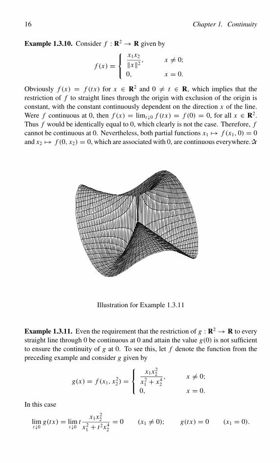
Illustration for Example 1.3.11
Example 1.3.11. Even the requirement that the restriction of g : R2 → R to everystraight line through 0 be continuous at 0 and attain the value g(0) is not sufficientto ensure the continuity of g at 0. To see this, let f denote the function from thepreceding example and consider g given by
g(x) = f (x1, x22) =
x1x2
2
x21 + x4
2
, x = 0;0, x = 0.
In this case
limt↓0
g(t x) = limt↓0
tx1x2
2
x21 + t2x4
2
= 0 (x1 = 0); g(t x) = 0 (x1 = 0).
1.4. Composition of mappings 17
Nevertheless, g still fails to be continuous at 0, as is obvious from
g(λ t2, t) = g(λ, 1) = λ
λ2 + 1∈ [ − 1
2,
1
2
](λ ∈ R, 0 = t ∈ R).
Consequently, the function g is constant on the parabolas { x ∈ R2 | x1 = λ x22 },
for λ ∈ R (whose union is R2 with the x1-axis excluded), and in each neighborhoodof 0 it assumes all values between − 1
2 and 12 . ✰
1.4 Composition of mappings
Definition 1.4.1. Let f : Rn ⊃→ Rp and g : Rp ⊃→ Rq . The compositiong ◦ f : Rn ⊃→ Rq has domain equal to dom( f )∩ f −1( dom(g)) and is defined by
(g ◦ f )(x) = g( f (x)).
In other words, it is the mapping
g ◦ f : x �→ f (x) �→ g( f (x)) : Rn ⊃→ Rp ⊃→ Rq .
In particular, let f1, f2 and f : Rn ⊃→ Rp and λ ∈ R. Then we define the sumf1+ f2 : Rn ⊃→ Rp and the scalar multiple λ f : Rn ⊃→ Rp as the compositions
f1 + f2 : x �→ ( f1(x), f2(x)) �→ f1(x)+ f2(x) : Rn ⊃→ R2p ⊃→ Rp,
λ f : x �→ (λ, f (x)) �→ λ f (x) : Rn ⊃→ Rp+1 ⊃→ Rp,
for x ∈⋂1≤k≤2 dom( fk) and x ∈ dom( f ), respectively. Next we define the product
〈 f1, f2〉 : Rn ⊃→ R as the composition
〈 f1, f2〉 : x �→ ( f1(x), f2(x)) �→ 〈 f1(x), f2(x)〉 : Rn ⊃→ Rp × Rp ⊃→ R,
for x ∈ ⋂1≤k≤2 dom( fk). Finally, assume p = 1. Then we write f1 f2 for the
product 〈 f1, f2〉 and define the reciprocal function 1f : Rn ⊃→ R by
1
f: x �→ f (x) �→ 1
f (x): Rn ⊃→ R ⊃→ R (x ∈ dom( f ) \ f −1({0})). ❍
Exactly as in the theory of real functions of one variable one obtains corre-sponding results for the limits and the continuity of these new mappings.
Theorem 1.4.2 (Substitution Theorem). Suppose f : Rn ⊃→ Rp and g : Rp ⊃→Rq; let a ∈ dom( f ), b ∈ dom(g) and c ∈ Rq , while limx→a f (x) = b andlimy→b g(y) = c. Then we have the following properties.
18 Chapter 1. Continuity
(i) limx→a(g ◦ f )(x) = c. In particular, if b ∈ dom(g) and g is continuous atb, then
limx→a
g( f (x)) = g( limx→a
f (x)).
(ii) Let a ∈ dom( f ) and f (a) ∈ dom(g). If f and g are continuous at a andf (a), respectively, then g ◦ f : Rn ⊃→ Rq is continuous at a.
Proof. Ad (i). Let W be an arbitrary neighborhood of c in Rq . A reformulation ofthe data by means of Proposition 1.3.2 gives the existence of a neighborhood V ofb in dom(g), and U of a in dom( f ) ∩ f −1( dom(g)), respectively, satisfying
V ⊂ g−1(W ), U ⊂ f −1(V ).
Combination of these inclusions proves the first equality in assertion (i), because
(g( f (U )) ⊂ g(V ) ⊂ W, thus U ⊂ (g ◦ f )−1(W ).
As for the interchange of the limit with the mapping g, note that
limx→a
g( f (x)) = limx→a
(g ◦ f )(x) = c = g(b) = g( limx→a
f (x)).
Assertion (ii) is a direct consequence of (i). ❏
The following corollary is immediate from the Substitution Theorem in con-junction with Example 1.3.5.
Corollary 1.4.3. For f1 and f2 : Rn ⊃→ Rp and λ ∈ R, we have the following.
(i) If a ∈ ⋂1≤k≤2 dom( fk), then limx→a(λ f1 + f2)(x) = λ limx→a f1(x) +
limx→a f2(x).
(ii) If a ∈ ⋂1≤k≤2 dom( fk) and f1 and f2 are continuous at a, then λ f1 + f2 is
continuous at a.
(iii) If a ∈ ⋂1≤k≤2 dom( fk), then we have limx→a〈 f1, f2〉(x) = 〈 limx→a f1(x),
limx→a f2(x)〉.(iv) If a ∈ ⋂
1≤k≤2 dom( fk) and f1 and f2 are continuous at a, then 〈 f1, f2〉 iscontinuous at a.
Furthermore, assume f : Rn ⊃→ R.
(v) If limx→a f (x) = 0, then limx→a1f (x) = 1
limx→a f (x) .
(vi) If a ∈ dom( f ), f (a) = 0 and f is continuous at a, then 1f is continuous at
a.
1.5. Homeomorphisms 19
Example 1.4.4. According to Lemma 1.1.7.(iv) the coordinate functions Rn → Rwith x �→ x j , for 1 ≤ j ≤ n, are continuous. It then follows from part (iv) in thecorollary above and by mathematical induction that monomial functions Rn → R,that is, functions of the form x �→ xα1
1 · · · xαnn , with α j ∈ N0 for 1 ≤ j ≤ n, are
continuous. In turn, this fact and part (ii) of the corollary imply that polynomial func-tions on Rn , which by definition are linear combinations of monomial functions onRn , are continuous. Furthermore, rational functions on Rn are defined as quotientsof polynomial functions on that subset of Rn where the quotient is well-defined.In view of parts (vi) and (iv) rational functions on Rn are continuous too. As thecomposition g ◦ f of a rational function f on Rn by a continuous function g on R isalso continuous by the Substitution Theorem 1.4.2.(ii), the continuity of functionson Rn that are given by formulae can often be decided by mere inspection. ✰
1.5 Homeomorphisms
Example 1.5.1. For functions f : R ⊃→ R we have the following result. LetI ⊂ R be an interval and let f : I → R be a continuous injective function. Thenf is strictly monotonic. The inverse function of f , which is defined on the intervalf (I ), is continuous and strictly monotonic. For instance, from the constructionof the trigonometric functions we know that tan : ]−π
2 ,π2
[ → R is a continuousbijection, hence it follows that the inverse function arctan : R → ]−π
2 ,π2
[is
continuous.However, for continuous mappings f : Rn ⊃→ Rp, with n ≥ 2, that are
bijective: dom( f ) → im( f ), the inverse is not automatically continuous. Forexample, consider f : ]−π, π ] → S1 := { x ∈ R2 | ‖x‖ = 1 } given by f (t) =(cos t, sin t). Then f is a continuous bijection, while
limt↓−π f (t) = lim
t↓−π(cos t, sin t) = (−1, 0) = f (π).
If f −1 : S1 → ]−π, π ] were continuous at (−1, 0) ∈ S1, then we would have bythe Substitution Theorem 1.4.2.(i)
π = f −1( f (π)) = f −1(
limt↓−π f (t)
)= lim
t↓−π t = −π. ✰
In order to describe phenomena like this we introduce the notion of a homeo-morphism (�µοος = similar and µορφ = shape).
Definition 1.5.2. Let A ⊂ Rn and B ⊂ Rp. A mapping f : A → B is saidto be a homeomorphism if f is a continuous bijection and the inverse mappingf −1 : B → A is continuous, that is, ( f −1)−1(O) = f (O) is open in B, for everyopen set O in A. If this is the case, A and B are called homeomorphic sets.
20 Chapter 1. Continuity
A mapping f : A → B is said to be open if the image under f of every openset in A is open in B, and f is said to be closed if the image under f of every closedset in A is closed in B. ❍
Example 1.5.3. In this terminology,]−π
2 ,π2
[and R are homeomorphic sets.
Let p < n. Then the orthogonal projection f : Rn → Rp with f (x) =(x1, . . . , x p) is a continuous open mapping. However, f is not closed; for example,consider f : R2 → R and the closed subset { x ∈ R2 | x1x2 = 1 }, which has thenonclosed image R \ {0} in R. ✰
Proposition 1.5.4. Let A ⊂ Rn and B ⊂ Rp and let f : A → B be a bijection.Then the following are equivalent.
(i) f is a homeomorphism.
(ii) f is continuous and open.
(iii) f is continuous and closed.
Proof. (i)⇔ (ii) follows from the definitions. For (i)⇔ (iii), use Formula (1.8).❏
At this stage the reader probably expects a theorem stating that, if U ⊂ Rn isopen and V ⊂ Rn and if f : U → V is a homeomorphism, then V is open in Rn .Indeed, under the further assumption of differentiability of f and of its inverse map-ping f −1, results of this kind will be established in this book, see Example 2.4.9 andSection 3.2. Moreover, Brouwer’s Theorem states that a continuous and injectivemapping f : U → Rn defined on an open set U ⊂ Rn is an open mapping. Relatedto this result is the invariance of dimension: if a neighborhood of a point in Rn ismapped continuously and injectively onto a neighborhood of a point in Rp, thenp = n. As yet, however, no proofs of these latter results are known at the level ofthis text. The condition of injectivity of the mapping is necessary for the invarianceof dimension, see Exercises 1.45 and 1.53, where it is demonstrated, surprisingly,that there exist continuous surjective mappings: I → I 2 with I = [ 0, 1 ] and thatthese never are injective.
1.6 Completeness
The more profound properties of continuous mappings turn out to be consequencesof the following.
1.6. Completeness 21
Theorem 1.6.1. Every nonempty set A ⊂ R which is bounded from above has asupremum or least upper bound a ∈ R, with notation a = sup A; that is, a has thefollowing properties:
(i) x ≤ a, for all x ∈ A;
(ii) for every δ > 0, there exists x ∈ A with a − δ < x.
Note that assertion (i) says that a is an upper bound for A while (ii) asserts thatno smaller number than a is an upper bound for A; therefore a is rightly called theleast upper bound for A. Similarly, we have the notion of an infimum or greatestlower bound.
Depending on one’s choice of the defining properties for the set R of realnumbers, Theorem 1.6.1 is either an axiom or indeed a theorem if the set R hasbeen constructed on the basis of other axioms. Here we take this theorem as thestarting point for our further discussions. A direct consequence is the Theorem ofBolzano–Weierstrass. For this we need a further definition.
We say that a sequence (xk)k∈N in Rn is bounded if there exists M > 0 suchthat ‖xk‖ ≤ M , for all k ∈ N.
Theorem 1.6.2 (Bolzano–Weierstrass on R). Every bounded sequence in R pos-sesses a convergent subsequence.
Proof. We denote our sequence by (xk)k∈N. Consider
a = sup A where A = { x ∈ R | x < xk for infinitely many k ∈ N }.
Then a ∈ R is well-defined because A is nonempty and bounded from above, as thesequence is bounded. Next let δ > 0 be arbitrary. By the definition of supremum,only a finite number of xk satisfy a + δ < xk , while there are infinitely many xk
with a − δ < xk in view of Theorem 1.6.1.(ii). Accordingly, we find infinitelymany k ∈ N with a − δ < xk < a + δ. Now successively select δ = 1
l with l ∈ N,and obtain a strictly increasing sequence of indices (kl)l∈N with |xkl − a| < 1
l . Thesubsequence (xkl )l∈N obviously converges to a. ❏
There is no straightforward extension of Theorem 1.6.1 to Rn because a rea-sonable ordering on Rn that is compatible with the vector operations does not existif n ≥ 2. Nevertheless, the Theorem of Bolzano–Weierstrass is quite easy to gen-eralize.
Theorem 1.6.3 (Bolzano–Weierstrass on Rn). Every bounded sequence in Rn
possesses a convergent subsequence.
22 Chapter 1. Continuity
Proof. Let (x (k))k∈N be our bounded sequence. We reduce to R by consideringthe sequence (x (k)1 )k∈N of first components, which is a bounded sequence in R.By the preceding theorem we then can extract a subsequence that is convergent inR. In order to prevent overburdening the notation we now assume that (x (k))k∈N
denotes the corresponding subsequence in Rn . The sequence (x (k)2 )k∈N of secondcomponents of that sequence is bounded in R too, and therefore we can extracta convergent subsequence. The corresponding subsequence in Rn now has theproperty that the sequences of both its first and second components converge. Wego on extracting subsequences; after the n-th extraction there are still infinitelymany terms left and we have a subsequence that converges in all components,which implies that it is convergent on the strength of Proposition 1.1.10. ❏
Definition 1.6.4. A sequence (xk)k∈N in Rn is said to be a Cauchy sequence if forevery ε > 0 there exists N ∈ N such that
k ≥ N and l ≥ N =⇒ ‖xk − xl‖ < ε. ❍
A Cauchy sequence is bounded. In fact, take ε = 1 in the definition above andlet N be the corresponding element in N. Then we obtain by the reverse triangleinequality from Lemma 1.1.7.(iii) that ‖xk‖ ≤ ‖xN‖ + 1, for all k ≥ N . Hence
‖xk‖ ≤ M := max{ ‖x1‖, . . . , ‖xN‖, ‖xN‖ + 1 }.Next, consider a sequence (xk)k∈N in Rn that converges to, say, a ∈ Rn . This is
a Cauchy sequence. Indeed, select ε > 0 arbitrarily. Then we can find N ∈ N with‖xk − a‖ < ε
2 , for all k ≥ N . Now the triangle inequality from Lemma 1.1.7.(i)implies, for all k and l ≥ N ,
‖xk − xl‖ ≤ ‖xk − a‖ + ‖xl − a‖ < ε
2+ ε
2= ε.
Note, however, that the definition of Cauchy sequence does not involve a limit,so that it is not immediately clear whether every Cauchy sequence has a limit. Infact, this is the case for Rn , but it is not true for every Cauchy sequence with termsin Qn , for instance.
Theorem 1.6.5 (Completeness of Rn). Every Cauchy sequence in Rn is convergentin Rn. This property of Rn is called its completeness.
Proof. A Cauchy sequence is bounded and thus it follows from the Theorem ofBolzano–Weierstrass that it has a subsequence convergent to a limit in Rn . But thenthe Cauchy property implies that the whole sequence converges to the same limit.❏
Note that the notions of Cauchy sequence and of completeness can be general-ized to arbitrary metric spaces in a straightforward fashion.
1.7. Contractions 23
1.7 Contractions
In this section we treat a first consequence of completeness.
Definition 1.7.1. Let F ⊂ Rn , let f : F → Rn be a mapping that is Lipschitzcontinuous with a Lipschitz constant ε < 1. Then f is said to be a contraction inF with contraction factor ≤ ε. In other words,
‖ f (x)− f (x ′)‖ ≤ ε‖x − x ′‖ < ‖x − x ′‖ (x, x ′ ∈ F). ❍
Lemma 1.7.2 (Contraction Lemma). Assume F ⊂ Rn closed and x0 ∈ F. Letf : F → F be a contraction with contraction factor ≤ ε. Then there exists aunique point x ∈ F with
f (x) = x; furthermore ‖x − x0‖ ≤ 1
1− ε‖ f (x0)− x0‖.
Proof. Because f is a mapping of F in F , a sequence (xk)k∈N0 in F may be definedinductively by
xk+1 = f (xk) (k ∈ N0).
By mathematical induction on k ∈ N0 it follows that
‖xk − xk+1‖ = ‖ f (xk−1)− f (xk)‖ ≤ ε‖xk−1 − xk‖ ≤ · · · ≤ εk‖x1 − x0‖.Repeated application of the triangle inequality then gives, for all m ∈ N,
‖xk − xk+m‖ ≤ ‖xk − xk+1‖ + · · · + ‖xk+m−1 − xk+m‖
≤ (1+ · · · + εm−1)εk ‖ f (x0)− x0‖ ≤ εk
1− ε‖ f (x0)− x0‖.
(1.9)
In other words, (xk)k∈N0 is a Cauchy sequence in F . Because of the completenessof Rn (see Theorem 1.6.5) there exists x ∈ Rn with limk→∞ xk = x ; and becauseF is closed, x ∈ F . Since f is continuous we therefore get from Lemma 1.3.6
f (x) = f ( limk→∞ xk) = lim
k→∞ f (xk) = limk→∞ xk+1 = x,
i.e. x is a fixed point of f . Also, x is the unique fixed point in F of f . Indeed,suppose x ′ is another fixed point in F , then
0 < ‖x − x ′‖ = ‖ f (x)− f (x ′)‖ < ‖x − x ′‖,which is a contradiction. Finally, in Inequality (1.9) we may take the limit form → ∞; in that way we obtain an estimate for the rate of convergence of thesequence (xk)k∈N0 :
‖xk − x‖ ≤ εk
1− ε‖ f (x0)− x0‖ (k ∈ N0). (1.10)
The last assertion in the lemma then follows for k = 0. ❏
24 Chapter 1. Continuity
Example 1.7.3. Let a ≥ 12 , and define F = [√
a2 ,∞
[and f : F → R by
f (x) = 1
2
(x + a
x
).
Then f (x) ∈ F for all x ∈ F , since (√
x − √ ax )2 ≥ 0 implies f (x) ≥ √
a.Furthermore,
−1
2≤ f ′(x) = 1
2
(1− a
x2
)≤ 1
2(x ∈ F).
Accordingly, application of the Mean Value Theorem on R (see Formula (2.14))yields that f is a contraction with contraction factor ≤ 1
2 . The fixed point forf equals
√a ∈ F . Using the estimate (1.10) we see that the sequence (xk)k∈N0
satisfies
|xk −√a| ≤ 2−k |a− 1| if x0 = a, xk+1 = 1
2
(xk + a
xk
)(k ∈ N).
In fact, the convergence is much stronger, as can be seen from
x2k+1 − a = 1
4x2k
(x2k − a)2 (k ∈ N0). (1.11)
Furthermore, this implies x2k+1 ≥ a, and from this it follows in turn that xk+2 ≤ xk+1,
i.e. the sequence (xk)k∈N0 decreases monotonically towards its limit√
a. ✰
For another proof of the Contraction Lemma based on Theorem 1.8.8 below,see Exercise 1.29.
If the appropriate estimates can be established, one may use the ContractionLemma to prove surjectivity of mappings f : Rn → Rn , for instance by consideringg : Rn → Rn with g(x) = x − f (x)+ y for a given y ∈ Rn . A fixed point x for gthen satisfies f (x) = y (this technique is applied in the proof of Proposition 3.2.3).In particular, taking y = 0 then leads to a zero x for f .
1.8 Compactness and uniform continuity
There is a class of infinite sets, called compact sets, that in certain limited aspectsbehave very much like finite sets. Consider the infinite pigeon-hole principle: if(xk)k∈N is a sequence in R all of whose terms belong to a finite set K , then at leastone element of K must be equal to xk for an infinite number of indices k. Forinfinite sets K this statement is obviously false. In this case, however, we couldhope for a slightly weaker conclusion: that K contains a point that is arbitrarilyclosely approximated, and this infinitely often. For many purposes in analysis suchan approximation is just as good as equality.
1.8. Compactness and uniform continuity 25
Definition 1.8.1. A set K ⊂ Rn is said to be compact (more precisely, sequen-tially compact) if every sequence of elements in K contains a subsequence whichconverges to a point in K . ❍
Later, in Definition 1.8.16, we shall encounter another definition of compact-ness, which is the standard one in more general spaces than Rn; in the latter, however,several different notions of compactness all coincide.
Note that the definition of compactness of K refers to the points of K only andto the distance function between the points in K , but does not refer to points outsideK . Therefore, compactness is an absolute concept, unlike the properties of beingopen or being closed, which depend on the ambient space Rn .
It is immediate from Definition 1.8.1 and Lemma 1.2.12 that we have the fol-lowing:
Lemma 1.8.2. A subset of a compact set K ⊂ Rn is compact if and only if it isclosed in K .
In Example 1.3.8 we saw that continuous mappings do not necessarily preserveclosed sets; on the other hand, they do preserve compact sets. In this sense compactand finite sets behave similarly: the image of a finite set under a mapping is a finiteset too.
Theorem 1.8.3 (Continuous image of compact is compact). Let K ⊂ Rn becompact and f : K → Rp a continuous mapping. Then f (K ) ⊂ Rp is compact.
Proof. Consider an arbitrary sequence (yk)k∈N of elements in f (K ). Then thereexists a sequence (xk)k∈N of elements in K with f (xk) = yk . By the compactness ofK the sequence (xk)k∈N contains a convergent subsequence, with limit a ∈ K , say.By going over to this subsequence, we have a = limk→∞ xk and from Lemma 1.3.6we get f (a) = limk→∞ f (xk) = limk→∞ yk . But this says that (yk)k∈N has aconvergent subsequence whose limit belongs to f (K ). ❏
Observe that there are two ingredients in the definition of compactness: onerelated to the Theorem of Bolzano–Weierstrass and thus to boundedness, viz., thata sequence has a convergent subsequence; and one related to closedness, viz., thatthe limit of a convergent sequence belongs to the set, see Lemma 1.2.12.(iii). Thesubsequent characterization of compact sets will be used throughout this book.
Theorem 1.8.4. For a set K ⊂ Rn the following assertions are equivalent.
(i) K is bounded and closed.
(ii) K is compact.
26 Chapter 1. Continuity
Proof. (i)⇒ (ii). Consider an arbitrary sequence (xk)k∈N of elements contained inK . As this sequence is bounded it has, by the Theorem of Bolzano–Weierstrass,a subsequence convergent to an element a ∈ Rn . Then a ∈ K according toLemma 1.2.12.(iii).(ii)⇒ (i). Assume K not bounded. Then we can find a sequence (xk)k∈N satisfyingxk ∈ K and ‖xk‖ ≥ k, for k ∈ N. Obviously, in this case the extraction of aconvergent subsequence is impossible, so that K cannot be compact. Finally, Kbeing closed follows from Lemma 1.2.12. Indeed, all subsequences of a convergentsequence converge to the same limit. ❏
It follows from the two preceding theorems that [−1, 1 ] and R are not home-omorphic; indeed, the former set is compact while the latter is not. On the otherhand, ]−1, 1 [ and R are homeomorphic, see Example 1.5.3.
Theorem 1.8.4 also implies that the inverse image of a compact set under acontinuous mapping is closed (see Theorem 1.3.7.(iii)); nevertheless, the inverseimage of a compact set might fail to be compact. For instance, consider f : Rn →{0}; or, more interestingly, f : R → R2 with f (t) = (cos t, sin t). Then the imageim( f ) = S1 := { x ∈ R2 | ‖x‖ = 1 }, which is compact in R2, but f −1(S1) = R,which is noncompact.
Definition 1.8.5. A mapping f : Rn → Rp is said to be proper if the inverse imageunder f of every compact set in Rp is compact in Rn , thus f −1(K ) ⊂ Rn compactfor every compact K ⊂ Rp. ❍
Intuitively, a proper mapping is one that maps points “near infinity” in Rn topoints “near infinity” in Rp.
Theorem 1.8.6. Let f : Rn → Rp be proper and continuous. Then f is a closedmapping.
Proof. Let F be a closed set in Rn . We verify that f (F) satisfies the conditionin Lemma 1.2.12.(iii). Indeed, let (xk)k∈N be a sequence of points in F with theproperty that ( f (xk))k∈N is convergent, with limit b ∈ Rp. Thus, for k sufficientlylarge, we have f (xk) ∈ K = { y ∈ Rp | ‖y − b‖ ≤ 1 }, while K is compact in Rp.This implies that xk ∈ f −1(K ) ∩ F ⊂ Rn , which is compact too, f being properand F being closed. Hence the sequence (xk)k∈N has a convergent subsequence,which we will also denote by (xk)k∈N, with limit a ∈ F . But then Lemma 1.3.6gives f (a) = limk→∞ f (xk) = b, that is b ∈ f (F). ❏
In Example 1.5.1 we saw that the inverse of a continuous bijection defined ona subset of Rn is not necessarily continuous. But for mappings with a compactdomain in Rn we do have a positive result.
1.8. Compactness and uniform continuity 27
Theorem 1.8.7. Suppose that K ⊂ Rn is compact, let L ⊂ Rp, and let f : K → Lbe a continuous bijective mapping. Then L is a compact set and f : K → L is ahomeomorphism.
Proof. Let F ⊂ K be closed in K . Proposition 1.2.17.(ii) then implies that Fis closed in Rn; and thus F is compact according to Lemma 1.8.2. Using Theo-rems 1.8.3 and 1.8.4 we see that f (F) is closed in Rp, and thus in L . The assertionof the theorem now follows from Proposition 1.5.4. ❏
Observe that this theorem also follows from Theorem 1.8.6.
Obviously, a scalar function on a finite set is bounded and attains its minimumand maximum values. In this sense compact sets resemble finite sets.
Theorem 1.8.8. Let K ⊂ Rn be a compact nonempty set, and let f : K → R be acontinuous function. Then there exist a and b ∈ K such that
f (a) ≤ f (x) ≤ f (b) (x ∈ K ).
Proof. f (K ) ⊂ R is a compact set by Theorem 1.8.3, and Theorem 1.8.4 thenimplies that sup f (K ) is well-defined. The definitions of supremum and of thecompactness of f (K ) then give that sup f (K ) ∈ f (K ). But this yields the existenceof the desired element b ∈ K . For a ∈ K consider inf f (K ). ❏
A useful application of this theorem is to show the equivalence of all norms onthe finite-dimensional vector space Rn . This implies that definitions formulated interms of the Euclidean norm, like those of limit and continuity in Section 1.3, or ofdifferentiability in Definition 2.2.2, are in fact independent of the particular choiceof the norm.
Definition 1.8.9. A norm on Rn is a function ν : Rn → R satisfying the followingconditions, for x , y ∈ Rn and λ ∈ R.
(i) Positivity: ν(x) ≥ 0, with equality if and only if x = 0.
(ii) Homogeneity: ν(λx) = |λ| ν(x).(iii) Triangle inequality: ν(x + y) ≤ ν(x)+ ν(y). ❍
Corollary 1.8.10 (Equivalence of norms on Rn). For every norm ν on Rn thereexist numbers c1 > 0 and c2 > 0 such that
c1‖x‖ ≤ ν(x) ≤ c2‖x‖ (x ∈ Rn).
In particular, ν is Lipschitz continuous, with c2 being a Lipschitz constant for ν.
28 Chapter 1. Continuity
Proof. We begin by proving the second inequality. From Formula (1.1) we havex =∑
1≤ j≤n x j e j ∈ Rn , and thus we obtain from the Cauchy–Schwarz inequality(see Proposition 1.1.6)
ν(x) = ν( ∑
1≤ j≤n
x j e j
)≤
∑1≤ j≤n
|x j | ν(e j ) ≤ ‖x‖ ‖(ν(e1), . . . , ν(en))‖ =: c2‖x‖.
Next we show that ν is Lipschitz continuous. Indeed, using ν(x) = ν(x−a+a) ≤ν(x − a)+ ν(a) we obtain
|ν(x)− ν(a)| ≤ ν(x − a) ≤ c2‖x − a‖ (x, a ∈ Rn).
Finally, we consider the restriction of ν to the compact K = { x ∈ Rn | ‖x‖ = 1 }.By Theorem 1.8.8 there exists a ∈ K with ν(a) ≤ ν(x), for all x ∈ K . Setc1 = ν(a), then c1 > 0 by Definition 1.8.9.(i). For arbitrary 0 = x ∈ Rn we have
1‖x‖ x ∈ K , and hence
c1 ≤ ν( 1
‖x‖ x)= ν(x)
‖x‖ . ❏
Definition 1.8.11. We denote by Aut(Rn) the set of bijective linear mappings orautomorphisms (α�τ�ς = of or by itself) of Rn into itself. ❍
Corollary 1.8.12. Let A ∈ Aut(Rn) and define ν : Rn → R by ν(x) = ‖Ax‖.Then ν is a norm on Rn and hence there exist numbers c1 > 0 and c2 > 0 satisfying
c1‖x‖ ≤ ‖Ax‖ ≤ c2‖x‖, c−12 ‖x‖ ≤ ‖A−1x‖ ≤ c−1
1 ‖x‖ (x ∈ Rn).
In the analysis in several real variables the notion of uniform continuity is asimportant as in the analysis in one variable. Roughly speaking, uniform continuityof a mapping f means that it is continuous and that the δ in Definition 1.3.4 appliesfor all a ∈ dom( f ) simultaneously.
Definition 1.8.13. Let f : Rn ⊃→ Rp be a mapping. Then f is said to be uniformlycontinuous if for every ε > 0 there exists δ > 0 satisfying
x, y ∈ dom( f ) and ‖x − y‖ < δ =⇒ ‖ f (x)− f (y)‖ < ε.
Equivalently, phrased in terms of neighborhoods: f is uniformly continuous if forevery neighborhood V of 0 in R p there exists a neighborhood U of 0 in Rn suchthat
x, y ∈ dom( f ) and x − y ∈ U =⇒ f (x)− f (y) ∈ V . ❍
1.8. Compactness and uniform continuity 29
Example 1.8.14. Any Lipschitz continuous mapping is uniformly continuous. Inparticular, every A ∈ Aut(Rn) is uniformly continuous; this follows directly fromCorollary 1.8.12. In fact, any linear mapping A : Rn → Rp, whether bijectiveor not, is Lipschitz continuous and therefore uniformly continuous. For a proof,observe that Formula (1.1) and Lemma 1.1.7.(iv) imply, for x ∈ Rn ,
‖Ax‖ = ‖∑
1≤ j≤n
x j Ae j‖ ≤∑
1≤ j≤n
|x j | ‖Ae j‖ ≤ ‖x‖∑
1≤ j≤n
‖Ae j‖ =: k‖x‖.
The function f : R → R with f (x) = x2 is not uniformly continuous. ✰
Theorem 1.8.15. Let K ⊂ Rn be compact and f : K → Rp a continuous mapping.Then f is uniformly continuous.
Proof. Suppose f is not uniformly continuous. Then there exists ε > 0 with thefollowing property. For every δ > 0 we can find a pair of points x and y ∈ K with‖x − y‖ < δ and nevertheless ‖ f (x)− f (y)‖ ≥ ε. In particular, for every k ∈ Nthere exist xk and yk ∈ K with
‖xk − yk‖ < 1
kand ‖ f (xk)− f (yk)‖ ≥ ε. (1.12)
By the compactness of K the sequence (xk)k∈N has a convergent subsequence,with a limit in K . Go over to this subsequence. Next (yk)k∈N has a convergentsubsequence, also with a limit in K . Again, we switch to this subsequence, toobtain a := limk→∞ xk and b := limk→∞ yk . Furthermore, by taking the limit inthe first inequality in (1.12) we see that a = b ∈ K . On the other hand, fromthe continuity of f at a we obtain limk→∞ f (xk) = f (a) = limk→∞ f (yk). Thecontinuity of the Euclidean norm then gives limk→∞ ‖ f (xk)− f (yk)‖ = 0; this isin contradiction with the second inequality in (1.12). ❏
In many cases a set K ⊂ Rn and a function f : K → R are known to possessa certain local property, that is, for every x ∈ K there exists a neighborhood U (x)of x in Rn such that the restriction of f to U (x) has the property in question. Forexample, continuity of f on K by definition has the following meaning: for everyε > 0 and every x ∈ K there exists an open neighborhood U (x) of x in Rn suchthat for all x ′ ∈ U (x) ∩ K one has | f (x) − f (x ′)| < ε. It then follows thatK ⊂ ⋃
x∈K U (x). Thus one finds collections of open sets in Rn with the propertythat K is contained in their union.
In such a case, one may wish to ascertain whether it follows that the set K , orthe function f , possesses the corresponding global property. The question may beasked, for example, whether f is uniformly continuous on K , that is, whether forevery ε > 0 there exists one open set U in Rn such that for all x , x ′ ∈ K withx − x ′ ∈ U one has | f (x) − f (x ′)| < ε. On the basis of Theorem 1.8.15 this
30 Chapter 1. Continuity
does indeed follow if K is compact. On the other hand, consider f (x) = 1x , for
x ∈ K := ] 0, 1 [. For every x ∈ K there exists a neighborhood U (x) of x in Rsuch that f |U (x) is bounded and such that K = ⋃
x∈K U (x), that is, f is locallybounded on K . Yet it is not true that f is globally bounded on K . This motivatesthe following:
Definition 1.8.16. A collection O = { Oi | i ∈ I } of open sets in Rn is said to bean open covering of a set K ⊂ Rn if
K ⊂⋃O∈O
O.
A subcollection O′ ⊂ O is said to be an (open) subcovering of K if O′ is a coveringof K ; if in addition O′ is a finite collection, it is said to be a finite (open) subcovering.
A subset K ⊂ Rn is said to be compact if every open covering of K contains afinite subcovering of K . ❍
In topology, this definition of compactness rather than the Definition 1.8.1 of(sequential) compactness is the proper one to use. In spaces like Rn , however, thetwo definitions 1.8.1 and 1.8.16 of compactness coincide, which is a consequenceof the following:
Theorem 1.8.17 (Heine–Borel). For a set K ⊂ Rn the following assertions areequivalent.
(i) K is bounded and closed.
(ii) K is compact in the sense of Definition 1.8.16.
The proof uses a technical concept.
Definition 1.8.18. An n-dimensional rectangle B parallel to the coordinate axes isa subset of Rn of the form
B = { x ∈ Rn | a j ≤ x j ≤ b j (1 ≤ j ≤ n) }where it is assumed that a j , b j ∈ R and a j ≤ b j , for 1 ≤ j ≤ n. ❍
Proof. (i) ⇒ (ii). Choose a rectangle B ⊂ Rn such that K ⊂ B. Then define, byinduction over k ∈ N0, a collection of rectangles Bk as follows. Let B0 = {B}and let Bk+1 be the collection of rectangles obtained by subdividing each rectangleB ∈ Bk into 2n rectangles by “halving the edges of B”.
Let O be an arbitrary open covering of K , and suppose that O does not contain afinite subcovering of K . Because K ⊂⋃
B1∈B1B1, there exists a rectangle B1 ∈ B1
1.8. Compactness and uniform continuity 31
such that O does not contain a finite subcovering of K ∩ B1 = ∅. But this impliesthe existence of a rectangle B2 with
B2 ∈ B2, B2 ⊂ B1, O contains no finite subcovering of K ∩ B2 = ∅.By induction over k we find a sequence of rectangles (Bk)k∈N such that
Bk ∈ Bk, Bk ⊂ Bk−1, O contains no finite subcovering of K ∩ Bk = ∅.(1.13)
Now let xk ∈ K ∩ Bk be arbitrary. Since Bk ⊂ Bl for k > l and since diameter Bl =2−l diameter B, we see that (xk)k∈N is a Cauchy sequence in Rn . In view of thecompleteness of Rn , see Theorem 1.6.5, this means that there exists x ∈ Rn suchthat x = limk→∞ xk ; since K is closed, we have x ∈ K . Thus there is O ∈ O withx ∈ O . Now O is open in Rn , and so we can find δ > 0 such that
B(x; δ) ⊂ O. (1.14)
Because limk→∞ diameter Bk = 0 and limk→∞ xk − x = 0, there is k ∈ N with
diameter Bk + ‖xk − x‖ < δ.
Let y ∈ Bk be arbitrary. Then
‖y − x‖ ≤ ‖y − xk‖ + ‖xk − x‖ ≤ diameter Bk + ‖xk − x‖ < δ;that is, y ∈ B(x; δ). But now it follows from (1.14) that Bk ⊂ O , which is incontradiction with (1.13). Therefore O must contain a finite subcovering of K .(ii)⇒ (i). The boundedness of K follows by covering K by open balls in Rn aboutthe origin of radius k, for k ∈ N. Now K admits of a finite subcovering by suchballs, from which it follows that K is bounded.
In order to demonstrate that K is closed, we prove that Rn \ K is open. Indeed,choose y /∈ K , and define O j = { x ∈ Rn | ‖x − y‖ > 1
j } for j ∈ N. This gives
K ⊂ Rn \ {y} =⋃j∈N
O j .
This open covering of the compact set K admits of a finite subcovering, and con-sequently
K ⊂⋃
1≤k≤l
O jk = O j0 if j0 = max{ jk | 1 ≤ k ≤ l }.
Therefore ‖x− y‖ > 1j0
if x ∈ K ; and so y ∈ { x ∈ Rn | ‖x− y‖ < 1j0} ⊂ Rn \K .❏
The proof of the next theorem is a characteristic application of compactness.
Theorem 1.8.19 (Dini’s Theorem). Let K ⊂ Rn be compact and suppose that thesequence ( fk)k∈N of continuous functions on K has the following properties.
32 Chapter 1. Continuity
(i) ( fk)k∈N converges pointwise on K to a continuous function f , in other words,limk→∞ fk(x) = f (x), for all x ∈ K .
(ii) ( fk)k∈N is monotonically decreasing, that is, fk(x) ≥ fk+1(x), for all k ∈ Nand x ∈ K .
Then ( fk)k∈N converges uniformly on K to the function f . More precisely, for everyε > 0 there exists N ∈ N such that we have
0 ≤ fk(x)− f (x) < ε (k ≥ N , x ∈ K ).
Proof. For each k ∈ N let gk = fk − f . Then gk is continuous on K , whilelimk→∞ gk(x) = 0 and gk(x) ≥ gk+1(x) ≥ 0, for all x ∈ K and k ∈ N. Let ε > 0be arbitrary and define Ok(ε) = g−1
k ( [ 0, ε [ ); note that Ok(ε) ⊂ Ol(ε) if k < l.Then the collection of sets { Ok(ε) | k ∈ N } is an open covering of K , because ofthe pointwise convergence of (gk)k∈N. By the compactness of K there exists a finitesubcovering. Let N be largest of the indices k labeling the sets in that subcovering,then K ⊂ ON (ε), and the assertion follows. ❏
To conclude this section we give an alternative characterization of the conceptof compactness.
Definition 1.8.20. Let K ⊂ Rn be a subset. A collection {Fi | i ∈ I } of sets in Rn
has the finite intersection property relative to K if for every finite subset J ⊂ I
K ∩⋂i∈J
Fi = ∅. ❍
Proposition 1.8.21. A set K ⊂ Rn is compact if and only if, for every collection{Fi | i ∈ I } of closed subsets in Rn having the finite intersection property relativeto K , we have
K ∩⋂i∈I
Fi = ∅.
Proof. In this proof O consistently represents a collection {Oi | i ∈ I } of opensubsets in Rn . For such O we define F = {Fi | i ∈ I } with Fi := Rn \ Oi ; then Fis a collection of closed subsets in Rn . Further, in this proof J invariably representsa finite subset of I . Now the following assertions (i) through (iv) are successivelyequivalent:
(i) K is not compact;
(ii) there exists O with K ⊂⋃i∈I Oi , and for every J one has K \⋃i∈J Oi = ∅;
1.9. Connectedness 33
(iii) there is O with Rn \ K ⊃ ⋂i∈I (R
n \ Oi ), and for every J one has K ∩⋂i∈J (R
n \ Oi ) = ∅;
(iv) there exists F with K ∩⋂i∈I Fi = ∅, and for every J one has K ∩⋂
i∈J Fi =∅.
In (ii)⇔ (iii) we used DeMorgan’s laws from (1.3). The assertion follows. ❏
1.9 Connectedness
Let I ⊂ R be an interval and f : I → R a continuous function. Then f has theintermediate value property, that is, f assumes on I all values in between any twoof the values it assumes; as a consequence f (I ) is an interval too. It is characteristicof open, or closed, intervals in R that these cannot be written as the union of twodisjoint open, or closed, subintervals, respectively. We take this indecomposabilityas a clue for generalization to Rn .
Definition 1.9.1. A set A ⊂ Rn is said to be disconnected if there exist open setsU and V in Rn such that
A∩U = ∅, A∩V = ∅, (A∩U )∩(A∩V ) = ∅, (A∩U )∪(A∩V ) = A.
In other words, A is the union of two disjoint nonempty subsets that are open in A.Furthermore, the set A is said to be connected if A is not disconnected. ❍
We recall the definition of an interval I contained in R: for every a and b ∈ Iand any c ∈ R the inequalities a < c < b imply that c ∈ I .
Proposition 1.9.2 (Connectedness of interval). The only connected subsets of Rcontaining more than one point are R and the intervals (open, closed, or half-open).
Proof. Let I ⊂ R be connected. If I were not an interval, then by definition theremust be a and b ∈ I and c /∈ I with a < c < b. Then I ∩ { x ∈ R | x < c } andI ∩ { x ∈ R | x > c } would be disjoint nonempty open subsets in I whose unionis I .
Let I ⊂ R be an interval. If I were not connected, then I = U ∪ V , where Uand V are disjoint nonempty open sets in I . Then there would be a ∈ U and b ∈ Vsatisfying a < b (rename if necessary). Define c = sup{ x ∈ R | [ a, x [ ⊂ U };then c ≤ b and thus c ∈ I , because I is an interval. Clearly c ∈ U
I; noting that
U = I \ V is closed in I , we must have c ∈ U . However, U is also open in I , andsince I is an interval there exists δ > 0 with ] c − δ, c + δ [ ⊂ U , which violatesthe definition of c. ❏
34 Chapter 1. Continuity
Lemma 1.9.3. The following assertions are equivalent for a set A ⊂ Rn.
(i) A is disconnected.
(ii) There exists a surjective continuous function sending A to the two-point set{0, 1}.
We recall the definition of the characteristic function 1A of a set A ⊂ Rn , with
1A(x) = 1 if x ∈ A, 1A(x) = 0 if x /∈ A.
Proof. For (i)⇒ (ii) use the characteristic function of A ∩U with U as in Defini-tion 1.9.1. It is immediate that (ii)⇒ (i). ❏
Theorem 1.9.4 (Continuous image of connected is connected). Let A ⊂ Rn beconnected and let f : A → Rp be a continuous mapping. Then f (A) is connectedin Rp.
Proof. If f (A) were disconnected, there would be a continuous surjection g :f (A)→ {0, 1}, and then g ◦ f : A → {0, 1}would also be a continuous surjection,violating the connectedness of A. ❏
Theorem 1.9.5 (Intermediate Value Theorem). Let A ⊂ Rn be connected and letf : A → R be a continuous function. Then f (A) is an interval in R; in particular,f takes on all values between any two that it assumes.
Proof. f (A) is connected in R according to Theorem 1.9.4, so by Proposition 1.9.2it is an interval. ❏
Lemma 1.9.6. The union of any family of connected subsets of Rn having at leastone point in common is also connected. Furthermore, the closure of a connectedset is connected.
Proof. Let x ∈ Rn and A = ∪α∈A Aα with x ∈ Aα and Aα ⊂ Rn connected.Suppose f : A → {0, 1} is continuous. Since each Aα is connected and x ∈ Aα,we have f (x ′) = f (x), for all x ′ ∈ Aα andα ∈ A. Thus f cannot be surjective. Forthe second assertion, let A ⊂ Rn be connected and f : A → {0, 1} be a continuousfunction. The continuity of f then implies that it cannot be surjective. ❏
1.9. Connectedness 35
Definition 1.9.7. Let A ⊂ Rn and x ∈ A. The connected component of x in A isthe union of all connected subsets of A containing x . ❍
Using the Lemmata 1.9.6 and 1.9.3 one easily proves the following:
Proposition 1.9.8. Let A ⊂ Rn and x ∈ A. Then we have the following assertions.
(i) The connected component of x in A is connected and is a maximal connectedset in A.
(ii) The connected component of x in A is closed in A.
(iii) The set of connected components of the points of A forms a partition of A, thatis, every point of A lies in a connected component, and different connectedcomponents are disjoint.
(iv) A continuous function f : A → {0, 1} is constant on the connected compo-nents of A.
Note that connected components of A need not be open subsets of A. Forinstance, consider the subset of the rationals Q in R. The connected component ofeach point x ∈ Q equals {x}.

Chapter 2
Differentiation
Locally, in shrinking neighborhoods of a point, a differentiable mapping can beapproximated by an affine mapping in such a way that the difference betweenthe two mappings vanishes faster than the distance to the point in question. Thiscondition forces the graphs of the original mapping and of the affine mapping to betangent at their point of intersection. The behavior of a differentiable mapping issubstantially better than that of a merely continuous mapping.
At this stage linear algebra starts to play an important role. We reformulate thedefinition of differentiability so that our earlier results on continuity can be usedto the full, thereby minimizing the need for additional estimates. The relationshipbetween being differentiable in this sense and possessing derivatives with respect toeach of the variables individually is discussed next. We develop rules for computingderivatives; among these, the chain rule for the derivative of a composition, inparticular, has many applications in subsequent parts of the book. A differentiablefunction has good properties as long as its derivative does not vanish; critical points,where the derivative vanishes, therefore deserve to be studied in greater detail.Higher-order derivatives and Taylor’s formula come next, because of their rolein determining the behavior of functions near critical points, as well as in manyother applications. The chapter closes with a study of the interaction between theoperations of taking a limit, of differentiation and of integration; in particular, weinvestigate conditions under which they may be interchanged.
2.1 Linear mappings
We begin by fixing our notation for linear mappings and matrices because no uni-versally accepted conventions exist. We denote by
Lin(Rn,Rp)
37
38 Chapter 2. Differentiation
the linear space of all linear mappings from Rn to Rp, thus A ∈ Lin(Rn,Rp) ifand only if
A : Rn → Rp, A(λx + y) = λAx + Ay (λ ∈ R, x, y ∈ Rn).
From linear algebra we know that, having chosen the standard basis (e1, . . . , en) inRn , we obtain the matrix of A as the rectangular array consisting of pn numbers inR, whose j-th column equals the element Ae j ∈ Rp, for 1 ≤ j ≤ n; that is
(Ae1 Ae2 · · · Ae j · · · Aen).
In other words, if (e′1, . . . , e′p) denotes the standard basis in Rp and if we write, seeFormula (1.1),
Ae j =∑
1≤i≤p
ai j e′i , then A has the matrix
a11 . . . a1n...
...
ap1 . . . apn
,
with p rows and n columns. The number ai j ∈ R is called the (i, j)-th entry orcoefficient of the matrix of A, with i labeling rows and j columns. In this book wewill sparingly use the matrix representation of a linear operator with respect to basesother than the standard bases. Nevertheless, we will keep the concepts of a lineartransformation and of its matrix representations separate, even though we will notdenote them in different ways, in order to avoid overburdening the notation. Write
Mat(p × n,R)
for the linear space of p × n matrices with coefficients in R. In the special casewhere n = p, we set
End(Rn) := Lin(Rn,Rn), Mat(n,R) := Mat(n × n,R).
Here End comes from endomorphism (�νδον = within).In Definition 1.8.11 we already encountered the special case of the subset of
the bijective elements in End(Rn), which are also called automorphisms of Rn . Wedenote this set, and the set of corresponding matrices by, respectively,
Aut(Rn) ⊂ End(Rn), GL(n,R) ⊂ Mat(n,R).
GL(n,R) is the general linear group of invertible matrices in Mat(n,R). In fact,composition of bijective linear mappings corresponds to multiplication of the as-sociated invertible matrices, and both operations satisfy the group axioms: thusAut(Rn) and GL(n,R) are groups, and they are noncommutative except in thecase of n = 1.
For practical purposes we identify the linear space Mat(p×n,R)with the linearspace Rpn by means of the bijective linear mapping c : Mat(p × n,R) → Rpn ,
2.1. Linear mappings 39
defined by
A = a11 . . . a1n
......
ap1 . . . apn
�→ c(A) := (a11, . . . , ap1, a12, . . . , ap2, . . . , apn).
(2.1)Observe that this map is obtained by putting the columns Ae j of A below eachother, and then writing the resulting vector as a row for typographical reasons. Wesummarize the results above in the following linear isomorphisms of vector spaces
Lin(Rn,Rp) � Mat(p × n,R) � Rpn. (2.2)
We now endow Lin(Rn,Rp)with a norm‖·‖Eucl, the Euclidean norm (also calledthe Frobenius norm or Hilbert–Schmidt norm), as follows. For A ∈ Lin(Rn,Rp)
we set
‖A‖Eucl := ‖c(A)‖ =√ ∑
1≤ j≤n
‖Ae j‖2 =√ ∑
1≤i≤p, 1≤ j≤n
a2i j . (2.3)
Intermezzo on linear algebra. There exists a more natural definition of the Eu-clidean norm. That definition, however, requires some notions from linear algebra.Since these will be needed in this book anyway, both in the theory and in the exer-cises, we recall them here.
Given A ∈ Lin(Rn,Rp), we have At ∈ Lin(Rp,Rn), the adjoint linear operatorof A with respect to the standard inner products on Rn and Rp. It is characterizedby the property
〈Ax, y〉 = 〈x, At y〉 (x ∈ Rn, y ∈ Rp).
It is immediate from ai j = 〈Ae j , ei 〉 = 〈e j , At ei 〉 = atji that the matrix of At with
respect to the standard basis of Rp, and that of Rn , is the transpose of the matrix of Awith respect to the standard basis of Rn , and that of Rp, respectively; in other words,it is obtained from the matrix of A by interchanging the rows with the columns.
For the standard basis (e1, . . . , en) in Rn we obtain
〈Aei , Ae j 〉 = 〈ei , (At A)e j 〉.Consequently, the composition At A ∈ End(Rn) has the symmetric matrix of innerproducts
(〈ai , a j 〉)1≤i, j≤n with a j = Ae j ∈ Rp, the j-th column of the matrix of A.(2.4)
This matrix is known as Gram’s matrix associated with the vectors a1, . . . , an ∈ Rp.Next, we recall the definition of tr A ∈ R, the trace of A ∈ End(Rn), as the
coefficient of −λn−1 in the following characteristic polynomial of A:
det(λI − A) = λn − λn−1 tr A + · · · + (−1)n det A.
40 Chapter 2. Differentiation
Now the multiplicative property of the determinant gives
det(λI − A) = det B(λI − A)B−1 = det(λI − B AB−1) (B ∈ Aut(Rn)),
and hence tr A = tr B AB−1. This makes it clear that tr A does not depend on aparticular matrix representation chosen for the operator A. Therefore, the trace canalso be computed by
tr A =∑
1≤ j≤n
a j j with (ai j ) ∈ Mat(n,R) a corresponding matrix.
With these definitions available it is obvious from (2.3) that
‖A‖2Eucl
=∑
1≤ j≤n
‖Ae j‖2 = tr(At A) (A ∈ Lin(Rn,Rp)).
Lemma 2.1.1. For all A ∈ Lin(Rn,Rp) and h ∈ Rn,
‖A h‖ ≤ ‖A‖Eucl ‖h‖. (2.5)
Proof. The Cauchy–Schwarz inequality from Proposition 1.1.6 immediately yields
‖A h‖2 =∑
1≤i≤p
( ∑1≤ j≤n
ai j h j
)2
≤∑
1≤i≤p
( ∑1≤ j≤n
a2i j
∑1≤k≤n
h2k
)= ‖A‖2
Eucl‖h‖2. ❏
The Euclidean norm of a linear operator A is easy to compute, but has thedisadvantage of not giving the best possible estimate in Inequality (2.5), whichwould be
inf{C ≥ 0 | ‖Ah‖ ≤ C‖h‖ for all h ∈ Rn }.It is easy to verify that this number is equal to the operator norm ‖A‖ of A, givenby
‖A‖ = sup{ ‖Ah‖ | h ∈ Rn, ‖h‖ = 1 }.In the general case the determination of ‖A‖ turns out to be a complicated problem.From Corollary 1.8.10 we know that the two norms are equivalent. More explicitly,using ‖Ae j‖ ≤ ‖A‖, for 1 ≤ j ≤ n, one sees
‖A‖ ≤ ‖A‖Eucl ≤√
n ‖A‖ (A ∈ Lin(Rn,Rp)).
See Exercise 2.66 for a proof by linear algebra of this estimate and of Lemma 2.1.1.In the linear space Lin(Rn,Rp) we can now introduce all concepts from Chap-
ter 1 with which we are already familiar for the Euclidean space Rpn . In particularwe now know what open and closed sets in Lin(Rn,Rp) are, and we know what ismeant by continuity of a mapping Rk ⊃→ Lin(Rn,Rp) or Lin(Rn,Rp)→ Rk . Inparticular, the mapping A �→ ‖A‖Eucl is continuous from Lin(Rn,Rp) to R.
Finally, we treat two results that are needed only later on, but for which we haveall the necessary concepts available at this stage.
2.1. Linear mappings 41
Lemma 2.1.2. Aut(Rn) is an open set of the linear space End(Rn), or equivalently,GL(n,R) is open in Mat(n,R).
Proof. We note that a matrix A belongs to GL(n,R) if and only if det A =0, and that A �→ det A is a continuous function on Mat(n,R), because it is apolynomial function in the coefficients of A. If therefore A0 ∈ GL(n,R), thereexists a neighborhood U of A0 in Mat(n,R) with det A = 0 if A ∈ U ; that is, withthe property that U ⊂ GL(n,R). ❏
Remark. Some more linear algebra leads to the following additional result. Wehave Cramer’s rule
det A · I = A A = AA (A ∈ Mat(n,R)). (2.6)
Here is A is the complementary matrix, given by
A = (ai j ) = ((−1)i− j det A ji ) ∈ Mat(n,R),
where Ai j ∈ Mat(n − 1,R) is the matrix obtained from A by deleting the i-th rowand the j-th column. (det Ai j is called the (i, j)-th minor of A.) In other words,with e j ∈ Rn denoting the j-th standard basis vector,
ai j = det(a1 · · · ai−1 e j ai+1 · · · an).
In fact, Cramer’s rule follows by expanding det A by rows and columns, respectively,and using the antisymmetric properties of the determinant. In particular, for A ∈GL(n,R), the inverse A−1 ∈ GL(n,R) is given by
A−1 = 1
det AA. (2.7)
The coefficients of A−1 are therefore rational functions of those of A, which impliesthe assertion in Lemma 2.1.2.
Definition 2.1.3. A ∈ End(Rn) is said to be self-adjoint if its adjoint At equals Aitself, that is, if
〈Ax, y〉 = 〈x, Ay〉 (x, y ∈ Rn).
We denote by End+(Rn) the linear subspace of End(Rn) consisting of the self-adjoint operators. For A ∈ End+(Rn), the corresponding matrix (ai j )1≤i, j≤n ∈Mat(n,R) with respect to any orthonormal basis for Rn is symmetric, that is, itsatisfies ai j = a ji , for 1 ≤ i, j ≤ n.
A ∈ End(Rn) is said to be anti-adjoint if A satisfies At = −A. We denote byEnd−(Rn) the linear subspace of End(Rn) consisting of the anti-adjoint operators.The corresponding matrices are antisymmetric, that is, they satisfy ai j = −a ji , for1 ≤ i, j ≤ n. ❍
42 Chapter 2. Differentiation
In the following lemma we show that End(Rn) splits into the direct sum of the±1 eigenspaces of the operation of taking the adjoint acting in this linear space.
Lemma 2.1.4. We have the direct sum decomposition
End(Rn) = End+(Rn)⊕ End−(Rn).
Proof. For every A ∈ End(Rn)we have A = 12 (A+At)+ 1
2 (A−At) ∈ End+(Rn)+End−(Rn). On the other hand, taking the adjoint of 0 = A+ + A− ∈ End+(Rn)+End−(Rn) gives 0 = A+ − A−, and thus A+ = A− = 0. ❏
2.2 Differentiable mappings
We briefly review the definition of differentiability of functions f : I → R definedon an interval I ⊂ R. Remember that f is said to be differentiable at a ∈ I if thelimit
limx→a
f (x)− f (a)
x − a=: f ′(a) ∈ R (2.8)
exists. Then f ′(a) is called the derivative of f at a, also denoted by D f (a) ord fdx (a).
Note that the definition of differentiability in (2.8) remains meaningful for amapping f : R → Rp; nevertheless, a direct generalization to f : Rn → Rp, forn ≥ 2, of this definition is not feasible: x − a is a vector in Rn , and it is impossibleto divide the vector f (x)− f (a) ∈ Rp by it. On the other hand, (2.8) is equivalentto
limx→a
f (x)− f (a)− f ′(a)(x − a)
x − a= 0,
which by the definition of limit is equivalent to
limx→a
| f (x)− f (a)− f ′(a)(x − a)||x − a| = 0.
This, however, involves a quotient of numbers in R, and hence the generalizationto mappings f : Rn ⊃→ Rp is straightforward.
As a motivation for results to come we formulate:
Proposition 2.2.1. Let f : I → R and a ∈ I . Then the following assertions areequivalent.
(i) f is differentiable at a.
(ii) There exists a function φ = φa : I → R continuous at a, such that
f (x) = f (a)+ φa(x)(x − a).
2.2. Differentiable mappings 43
(iii) There exist a number L(a) ∈ R and a function εa : R ⊃→ R, such that, forh ∈ R with a + h ∈ I ,
f (a + h) = f (a)+ L(a) h + εa(h) with limh→0
εa(h)
h= 0.
If one of these conditions is satisfied, we have
f ′(a) = φa(a) = L(a), φa(x) = f ′(a)+ εa(x − a)
x − a(x = a). (2.9)
Proof. (i)⇒ (ii). Define
φa(x) =
f (x)− f (a)
x − a, x ∈ I \ {a};
f ′(a), x = a.
Then, indeed, we have f (x) = f (a) + (x − a)φa(x) and φa is continuous at a,because
φa(a) = f ′(a) = limx→a
f (x)− f (a)
x − a= lim
x→a, x =aφa(x).
(ii)⇒ (iii). We can take L(a) = φa(a) and εa(h) = (φa(a + h)− φa(a))h.(iii)⇒ (i). Straightforward. ❏
In the theory of differentiation of functions depending on several variables it isessential to consider limits for x ∈ Rn freely approaching a ∈ Rn , from all possibledirections; therefore, in what follows, we require our mappings to be defined onopen sets. We now introduce:
Definition 2.2.2. Let U ⊂ Rn be an open set, let a ∈ U and f : U → Rp. Thenf is said to be a differentiable mapping at a if there exists D f (a) ∈ Lin(Rn,Rp)
such that
limx→a
‖ f (x)− f (a)− D f (a)(x − a)‖‖x − a‖ = 0.
D f (a) is said to be the (total) derivative of f at a. Indeed, in Lemma 2.2.3 below,we will verify that D f (a) is uniquely determined once it exists. We say that f isdifferentiable if it is differentiable at every point of its domain U . In that case thederivative or derived mapping D f of f is the operator-valued mapping defined by
D f : U → Lin(Rn,Rp) with a �→ D f (a). ❍
In other words, in this definition we require the existence of a mapping εa :Rn ⊃→ Rp satisfying, for all h with a + h ∈ U ,
f (a + h) = f (a)+ D f (a)h + εa(h) with limh→0
‖εa(h)‖‖h‖ = 0. (2.10)
44 Chapter 2. Differentiation
In the case where n = p = 1, the mapping L �→ L(1) gives a linear isomorphismEnd(R)
∼−→ R. This new definition of the derivative D f (a) ↔ D f (a)1 ∈ Rtherefore coincides (up to isomorphism) with the original f ′(a) ∈ R.
Lemma 2.2.3. D f (a) ∈ Lin(Rn,Rp) is uniquely determined if f as above isdifferentiable at a.
Proof. Consider any h ∈ Rn . For t ∈ R with |t | sufficiently small we havea + th ∈ U and hence, by Formula (2.10),
D f (a)h = 1
t( f (a + th)− f (a))− 1
tεa(th).
It then follows, again by (2.10), that D f (a)h = limt→01t ( f (a + th) − f (a)); in
particular D f (a)h is completely determined by f . ❏
Definition 2.2.4. If f as above is differentiable at a, then we say that the mapping
Rn → Rp given by x �→ f (a)+ D f (a)(x − a)
is the best affine approximation to f at a. It is the unique affine approximation forwhich the difference mapping εa satisfies the estimate in (2.10). ❍
In Chapter 5 we will define the notion of a geometric tangent space and in Theo-rem 5.1.2 we will see that the geometric tangent space of graph( f ) = { (x, f (x)) ∈Rn+p | x ∈ dom( f ) } at (a, f (a)) equals the graph { (x, f (a)+ D f (a)(x − a)) ∈Rn+p | x ∈ Rn } of the best affine approximation to f at a. For n = p = 1, thisgives the familiar concept of the geometric tangent line at a point to the graph of f .
Example 2.2.5. (Compare with Example 1.3.5.) Every A ∈ Lin(Rn,Rp) is differ-entiable and we have D A(a) = A, for all a ∈ Rn . Indeed, A(a+h)−A(a) = A(h),for every h ∈ Rn; and there is no remainder term. (Of course, the best affine ap-proximation of a linear mapping is the mapping itself.) The derivative of A isthe constant mapping D A : Rn → Lin(Rn,Rp) with D A(a) = A. For exam-ple, the derivative of the identity mapping I ∈ Aut(Rn) with I (x) = x satisfiesDI = I . Furthermore, as the mapping: Rn × Rn → Rn of addition, given by(x1, x2) �→ x1 + x2, is linear, it is its own derivative.
Next, define g : Rn×Rn → R by g(x1, x2) = 〈x1, x2〉. Then g is differentiablewhile Dg(a1, a2) ∈ Lin(Rn × Rn,R) is the mapping satisfying
Dg(a1, a2)(h1, h2) = 〈a1, h2〉 + 〈a2, h1〉 (a1, a2, h1, h2 ∈ Rn).
2.2. Differentiable mappings 45
Indeed,
g(a1 + h1, a2 + h2)− g(a1, a2) = 〈h1, a2〉 + 〈a1, h2〉 + 〈h1, h2〉 with
0 ≤ lim(h1,h2)→0
|〈h1, h2〉|‖(h1, h2)‖ ≤ lim
(h1,h2)→0
‖h1‖ ‖h2‖‖(h1, h2)‖ ≤ lim
(h1,h2)→0‖h2‖ = 0.
Here we used the Cauchy–Schwarz inequality from Proposition 1.1.6 and the esti-mate (1.7).
Finally, let f1 and f2 : Rn → Rp be differentiable and define f : Rn → Rp×Rp
by f (x) = ( f1(x), f2(x)). Then f is differentiable and D f (a) ∈ Lin(Rn,Rp×Rp)
is given by
D f (a)h = (D f1(a)h, D f2(a)h) (a, h ∈ Rn). ✰
Example 2.2.6. Let U ⊂ Rn be open, let a ∈ U and let f : U → Rn bedifferentiable at a. Suppose D f (a) ∈ Aut(Rn). Then a is an isolated zero forf − f (a), which means that there exists a neighborhood U1 of a in U such thatx ∈ U1 and f (x) = f (a) imply x = a. Indeed, applying part (i) of the SubstitutionTheorem 1.4.2 with the linear and thus continuous D f (a)−1 : Rn → Rn (seeExample 1.8.14), we also have
limh→0
1
‖h‖D f (a)−1εa(h) = 0.
Therefore we can select δ > 0 such that ‖D f (a)−1εa(h)‖ < ‖h‖, for 0 < ‖h‖ < δ.This said, consider a + h ∈ U with 0 < ‖h‖ < δ and f (a + h) = f (a). ThenFormula (2.10) gives
0 = D f (a)h + εa(h), and thus ‖h‖ = ‖D f (a)−1εa(h)‖ < ‖h‖,and this contradiction proves the assertion. In Proposition 3.2.3 we shall return tothis theme. ✰
As before we obtain:
Lemma 2.2.7 (Hadamard). Let U ⊂ Rn be an open set, let a ∈ U and f : U →Rp. Then the following assertions are equivalent.
(i) The mapping f is differentiable at a.
(ii) There exists an operator-valued mapping φ = φa : U → Lin(Rn,Rp)
continuous at a, such that
f (x) = f (a)+ φa(x)(x − a).
46 Chapter 2. Differentiation
If one of these conditions is satisfied we have φa(a) = D f (a).
Proof. (i) ⇒ (ii). In the notation of Formula (2.10) we define (compare withFormula (2.9))
φa(x) = D f (a)+ 1
‖x − a‖2εa(x − a)(x − a)t , x ∈ U \ {a};
D f (a), x = a.
Observe that the matrix product of the column vector εa(x − a) ∈ Rp with the rowvector (x − a)t ∈ Rn yields a p × n matrix, which is associated with a mapping inLin(Rn,Rp). Or, in other words, since (x − a)t y = 〈x − a, y〉 ∈ R for y ∈ Rn ,
φa(x)y = D f (a)y + 〈x − a, y〉‖x − a‖2
εa(x − a) ∈ Rp (x ∈ U \ {a}, y ∈ Rn).
Now, indeed, we have f (x) = f (a) + φa(x)(x − a). A direct computation gives‖εa(h) ht‖Eucl = ‖εa(h)‖ ‖h‖, hence
limh→0
‖εa(h) ht‖Eucl
‖h‖2= lim
h→0
‖εa(h)‖‖h‖ = 0.
This shows that φa is continuous at a.(ii)⇒ (i). Straightforward upon using Lemma 2.1.1. ❏
From the representation of f in Hadamard’s Lemma 2.2.7.(ii) we obtain at once:
Corollary 2.2.8. f is continuous at a if f is differentiable at a.
Once more Lemma 1.1.7.(iv) implies:
Proposition 2.2.9. Let U ⊂ Rn be an open set, let a ∈ U and f : U → Rp. Thenthe following assertions are equivalent.
(i) The mapping f is differentiable at a.
(ii) Every component function fi : U → R of f , for 1 ≤ i ≤ p, is differentiableat a.
2.3. Directional and partial derivatives 47
2.3 Directional and partial derivatives
Suppose f to be differentiable at a and let 0 = v ∈ Rn be fixed. Then we can applyFormula (2.10) with h = tv for t ∈ R. Since D f (a) ∈ Lin(Rn,Rp), we find
f (a + tv)− f (a)− t D f (a)v = εa(tv),
limt→0‖εa(tv)‖|t | = ‖v‖ lim
tv→0
‖εa(tv)‖‖tv‖ = 0.
(2.11)
This says that the mapping g : R ⊃→ Rp given by g(t) = f (a+tv) is differentiableat 0 with derivative g′(0) = D f (a)v ∈ Rp.
Definition 2.3.1. Let U ⊂ Rn be an open set, let a ∈ U and f : U → Rp. Wesay that f has a directional derivative at a in the direction of v ∈ Rn if the functionR ⊃→ Rp with t �→ f (a + tv) is differentiable at 0. In that case
d
dt
∣∣∣∣t=0
f (a + tv) = limt→0
1
t( f (a + tv)− f (a)) =: Dv f (a) ∈ Rp
is called the directional derivative of f at a in the direction of v.In the particular case where v is equal to the standard basis vector e j ∈ Rn , for
1 ≤ j ≤ n, we callDe j f (a) =: D j f (a) ∈ Rp
the j-th partial derivative of f at a. If all n partial derivatives of f at a exist wesay that f is partially differentiable at a. Finally, f is called partially differentiableif it is so at every point of U . ❍
Note that
D j f (a) = d
dt
∣∣∣∣t=a j
f (a1, . . . , a j−1, t, a j+1, . . . , an).
This is the derivative of the j-th partial mapping associated with f and a, for whichthe remaining variables are kept fixed.
Proposition 2.3.2. Let f be as in Definition 2.3.1. If f is differentiable at a it hasthe following properties.
(i) f has directional derivatives at a in all directions v ∈ Rn and Dv f (a) =D f (a)v. In particular, the mapping Rn → Rp given by v �→ Dv f (a) islinear.
(ii) f is partially differentiable at a and
D f (a)v =∑
1≤ j≤n
v j D j f (a) (v ∈ Rn).
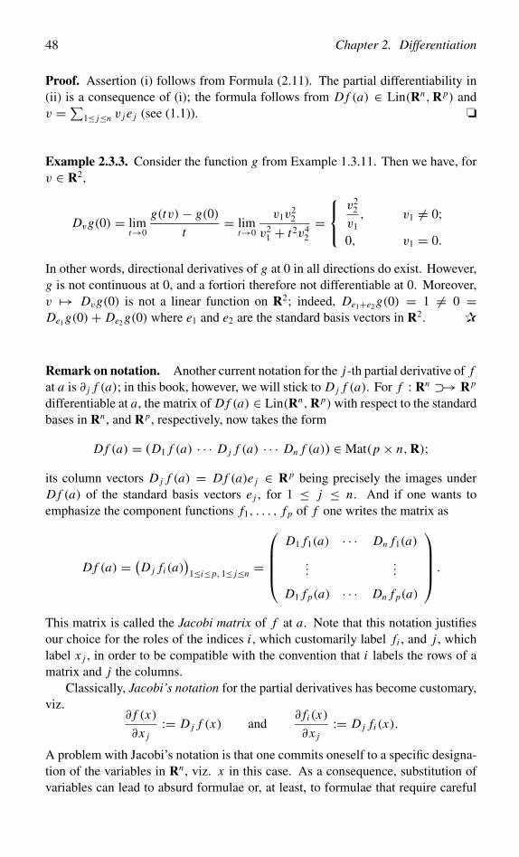
48 Chapter 2. Differentiation
Proof. Assertion (i) follows from Formula (2.11). The partial differentiability in(ii) is a consequence of (i); the formula follows from D f (a) ∈ Lin(Rn,Rp) andv =∑
1≤ j≤n v j e j (see (1.1)). ❏
Example 2.3.3. Consider the function g from Example 1.3.11. Then we have, forv ∈ R2,
Dvg(0) = limt→0
g(tv)− g(0)
t= lim
t→0
v1v22
v21 + t2v4
2
=
v22
v1, v1 = 0;
0, v1 = 0.
In other words, directional derivatives of g at 0 in all directions do exist. However,g is not continuous at 0, and a fortiori therefore not differentiable at 0. Moreover,v �→ Dvg(0) is not a linear function on R2; indeed, De1+e2 g(0) = 1 = 0 =De1 g(0)+ De2 g(0) where e1 and e2 are the standard basis vectors in R2. ✰
Remark on notation. Another current notation for the j-th partial derivative of fat a is ∂ j f (a); in this book, however, we will stick to D j f (a). For f : Rn ⊃→ Rp
differentiable at a, the matrix of D f (a) ∈ Lin(Rn,Rp) with respect to the standardbases in Rn , and Rp, respectively, now takes the form
D f (a) = (D1 f (a) · · · D j f (a) · · · Dn f (a)) ∈ Mat(p × n,R);its column vectors D j f (a) = D f (a)e j ∈ Rp being precisely the images underD f (a) of the standard basis vectors e j , for 1 ≤ j ≤ n. And if one wants toemphasize the component functions f1, . . . , f p of f one writes the matrix as
D f (a) = (D j fi (a)
)1≤i≤p, 1≤ j≤n
=
D1 f1(a) · · · Dn f1(a)
......
D1 f p(a) · · · Dn f p(a)
.
This matrix is called the Jacobi matrix of f at a. Note that this notation justifiesour choice for the roles of the indices i , which customarily label fi , and j , whichlabel x j , in order to be compatible with the convention that i labels the rows of amatrix and j the columns.
Classically, Jacobi’s notation for the partial derivatives has become customary,viz.
∂ f (x)
∂x j:= D j f (x) and
∂ fi (x)
∂x j:= D j fi (x).
A problem with Jacobi’s notation is that one commits oneself to a specific designa-tion of the variables in Rn , viz. x in this case. As a consequence, substitution ofvariables can lead to absurd formulae or, at least, to formulae that require careful
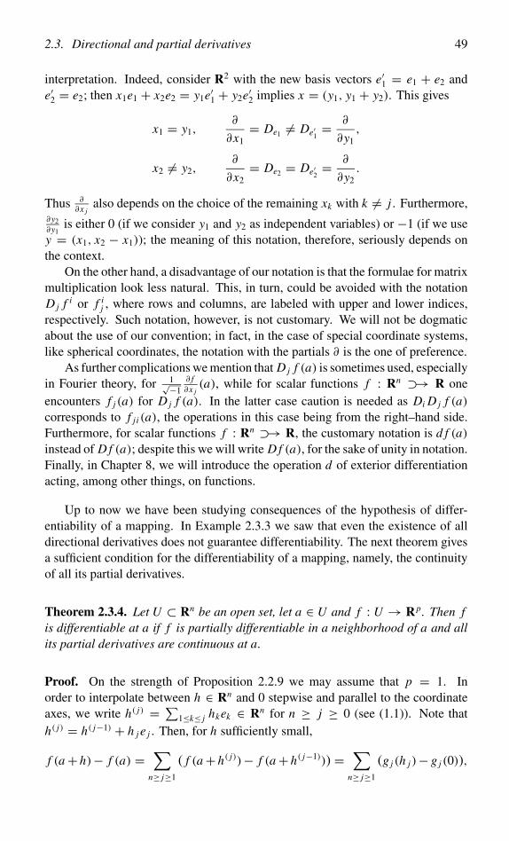
2.3. Directional and partial derivatives 49
interpretation. Indeed, consider R2 with the new basis vectors e′1 = e1 + e2 ande′2 = e2; then x1e1 + x2e2 = y1e′1 + y2e′2 implies x = (y1, y1 + y2). This gives
x1 = y1,∂
∂x1= De1 = De′1 =
∂
∂y1,
x2 = y2,∂
∂x2= De2 = De′2 =
∂
∂y2.
Thus ∂∂x j
also depends on the choice of the remaining xk with k = j . Furthermore,∂y2∂y1
is either 0 (if we consider y1 and y2 as independent variables) or −1 (if we usey = (x1, x2 − x1)); the meaning of this notation, therefore, seriously depends onthe context.
On the other hand, a disadvantage of our notation is that the formulae for matrixmultiplication look less natural. This, in turn, could be avoided with the notationD j f i or f i
j , where rows and columns, are labeled with upper and lower indices,respectively. Such notation, however, is not customary. We will not be dogmaticabout the use of our convention; in fact, in the case of special coordinate systems,like spherical coordinates, the notation with the partials ∂ is the one of preference.
As further complications we mention that D j f (a) is sometimes used, especiallyin Fourier theory, for 1√−1
∂ f∂x j(a), while for scalar functions f : Rn ⊃→ R one
encounters f j (a) for D j f (a). In the latter case caution is needed as Di D j f (a)corresponds to f ji (a), the operations in this case being from the right–hand side.Furthermore, for scalar functions f : Rn ⊃→ R, the customary notation is d f (a)instead of D f (a); despite this we will write D f (a), for the sake of unity in notation.Finally, in Chapter 8, we will introduce the operation d of exterior differentiationacting, among other things, on functions.
Up to now we have been studying consequences of the hypothesis of differ-entiability of a mapping. In Example 2.3.3 we saw that even the existence of alldirectional derivatives does not guarantee differentiability. The next theorem givesa sufficient condition for the differentiability of a mapping, namely, the continuityof all its partial derivatives.
Theorem 2.3.4. Let U ⊂ Rn be an open set, let a ∈ U and f : U → Rp. Then fis differentiable at a if f is partially differentiable in a neighborhood of a and allits partial derivatives are continuous at a.
Proof. On the strength of Proposition 2.2.9 we may assume that p = 1. Inorder to interpolate between h ∈ Rn and 0 stepwise and parallel to the coordinateaxes, we write h( j) = ∑
1≤k≤ j hkek ∈ Rn for n ≥ j ≥ 0 (see (1.1)). Note thath( j) = h( j−1) + h j e j . Then, for h sufficiently small,
f (a+ h)− f (a) =∑
n≥ j≥1
( f (a+ h( j))− f (a+ h( j−1))) =∑
n≥ j≥1
(g j (h j )− g j (0)),
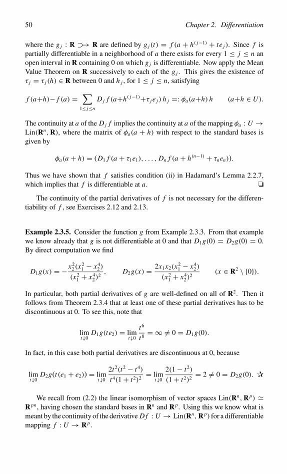
50 Chapter 2. Differentiation
where the g j : R ⊃→ R are defined by g j (t) = f (a + h( j−1) + te j ). Since f ispartially differentiable in a neighborhood of a there exists for every 1 ≤ j ≤ n anopen interval in R containing 0 on which g j is differentiable. Now apply the MeanValue Theorem on R successively to each of the g j . This gives the existence ofτ j = τ j (h) ∈ R between 0 and h j , for 1 ≤ j ≤ n, satisfying
f (a+h)− f (a) =∑
1≤ j≤n
D j f (a+h( j−1)+τ j e j ) h j =: φa(a+h) h (a+h ∈ U ).
The continuity at a of the D j f implies the continuity at a of the mapping φa : U →Lin(Rn,R), where the matrix of φa(a + h) with respect to the standard bases isgiven by
φa(a + h) = (D1 f (a + τ1e1), . . . , Dn f (a + h(n−1) + τnen)).
Thus we have shown that f satisfies condition (ii) in Hadamard’s Lemma 2.2.7,which implies that f is differentiable at a. ❏
The continuity of the partial derivatives of f is not necessary for the differen-tiability of f , see Exercises 2.12 and 2.13.
Example 2.3.5. Consider the function g from Example 2.3.3. From that examplewe know already that g is not differentiable at 0 and that D1g(0) = D2g(0) = 0.By direct computation we find
D1g(x) = − x22(x
21 − x4
2)
(x21 + x4
2)2, D2g(x) = 2x1x2(x2
1 − x42)
(x21 + x4
2)2
(x ∈ R2 \ {0}).
In particular, both partial derivatives of g are well-defined on all of R2. Then itfollows from Theorem 2.3.4 that at least one of these partial derivatives has to bediscontinuous at 0. To see this, note that
limt↓0
D1g(te2) = limt↓0
t6
t8= ∞ = 0 = D1g(0).
In fact, in this case both partial derivatives are discontinuous at 0, because
limt↓0
D2g(t (e1 + e2)) = limt↓0
2t2(t2 − t4)
t4(1+ t2)2= lim
t↓0
2(1− t2)
(1+ t2)2= 2 = 0 = D2g(0). ✰
We recall from (2.2) the linear isomorphism of vector spaces Lin(Rn,Rp) �Rpn , having chosen the standard bases in Rn and Rp. Using this we know what ismeant by the continuity of the derivative D f : U → Lin(Rn,Rp) for a differentiablemapping f : U → Rp.
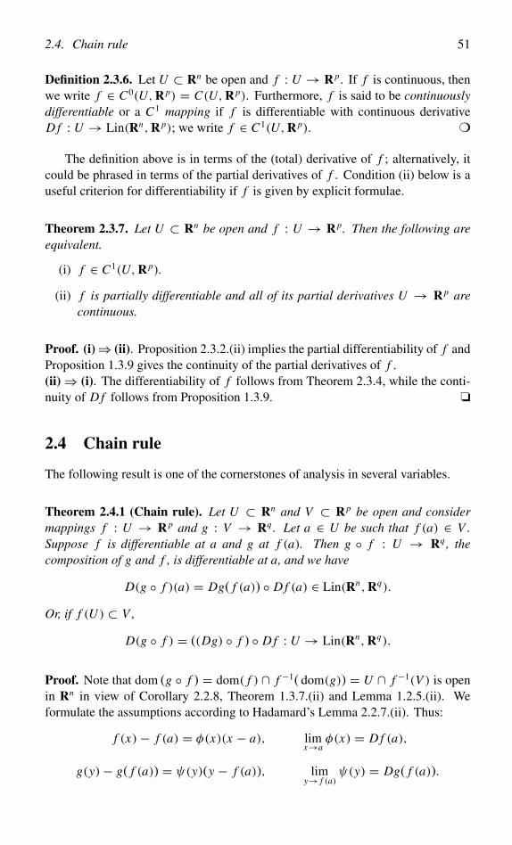
2.4. Chain rule 51
Definition 2.3.6. Let U ⊂ Rn be open and f : U → Rp. If f is continuous, thenwe write f ∈ C0(U,Rp) = C(U,Rp). Furthermore, f is said to be continuouslydifferentiable or a C1 mapping if f is differentiable with continuous derivativeD f : U → Lin(Rn,Rp); we write f ∈ C1(U,Rp). ❍
The definition above is in terms of the (total) derivative of f ; alternatively, itcould be phrased in terms of the partial derivatives of f . Condition (ii) below is auseful criterion for differentiability if f is given by explicit formulae.
Theorem 2.3.7. Let U ⊂ Rn be open and f : U → Rp. Then the following areequivalent.
(i) f ∈ C1(U,Rp).
(ii) f is partially differentiable and all of its partial derivatives U → Rp arecontinuous.
Proof. (i)⇒ (ii). Proposition 2.3.2.(ii) implies the partial differentiability of f andProposition 1.3.9 gives the continuity of the partial derivatives of f .(ii) ⇒ (i). The differentiability of f follows from Theorem 2.3.4, while the conti-nuity of D f follows from Proposition 1.3.9. ❏
2.4 Chain rule
The following result is one of the cornerstones of analysis in several variables.
Theorem 2.4.1 (Chain rule). Let U ⊂ Rn and V ⊂ Rp be open and considermappings f : U → Rp and g : V → Rq . Let a ∈ U be such that f (a) ∈ V .Suppose f is differentiable at a and g at f (a). Then g ◦ f : U → Rq , thecomposition of g and f , is differentiable at a, and we have
D(g ◦ f )(a) = Dg( f (a)) ◦ D f (a) ∈ Lin(Rn,Rq).
Or, if f (U ) ⊂ V ,
D(g ◦ f ) = ((Dg) ◦ f ) ◦ D f : U → Lin(Rn,Rq).
Proof. Note that dom (g ◦ f ) = dom( f ) ∩ f −1( dom(g)) = U ∩ f −1(V ) is openin Rn in view of Corollary 2.2.8, Theorem 1.3.7.(ii) and Lemma 1.2.5.(ii). Weformulate the assumptions according to Hadamard’s Lemma 2.2.7.(ii). Thus:
f (x)− f (a) = φ(x)(x − a), limx→a
φ(x) = D f (a),
g(y)− g( f (a)) = ψ(y)(y − f (a)), limy→ f (a)
ψ(y) = Dg( f (a)).
52 Chapter 2. Differentiation
Putting y = f (x) and inserting the first equation into the second one, we find
(g ◦ f )(x)− (g ◦ f )(a) = ψ( f (x))φ(x)(x − a).
Furthermore, limx→a f (x) = f (a) and limy→ f (a) ψ(y) = Dg( f (a)) give, in viewof the Substitution Theorem 1.4.2.(i)
limx→a
ψ( f (x)) = Dg( f (a)).
Therefore Corollary 1.4.3 implies
limx→a
ψ( f (x))φ(x) = limx→a
ψ( f (x)) limx→a
φ(x) = Dg( f (a))D f (a).
But then the implication (ii) ⇒ (i) from Hadamard’s Lemma 2.2.7 says that g ◦ fis differentiable at a and that D(g ◦ f )(a) = Dg( f (a))D f (a). ❏
Corollary 2.4.2 (Chain rule for Jacobi matrices). Let f and g be as in Theo-rem 2.4.1. In terms of the coefficients of the corresponding Jacobi matrices thechain rule takes the form, because (g ◦ f )i = gi ◦ f ,
D j (gi ◦ f ) =∑
1≤k≤p
((Dk gi ) ◦ f )D j fk (1 ≤ j ≤ n, 1 ≤ i ≤ q).
Denoting the variable in Rn by x, and the one in Rp by y, we obtain in Jacobi’snotation for partial derivatives
∂(gi ◦ f )
∂x j=
∑1≤k≤p
( ∂gi
∂yk◦ f
) ∂ fk
∂x j(1 ≤ i ≤ q, 1 ≤ j ≤ n).
In this context, it is customary to write yk = fk(x1, . . . , xn) and zi = gi (y1, . . . , yp),and write the chain rule (suppressing the points at which functions are to be eval-uated) in the form
∂zi
∂x j=
∑1≤k≤p
∂zi
∂yk
∂yk
∂x j(1 ≤ i ≤ q, 1 ≤ j ≤ n).
Proof. The first formula is immediate from the expression
hi j =∑
1≤k≤p
gik fk j (1 ≤ i ≤ q, 1 ≤ j ≤ n)
for the coefficients of a matrix H = G F ∈ Mat(q × n,R) which is the product ofG ∈ Mat(q × p,R) and F ∈ Mat(p × n,R). ❏
2.4. Chain rule 53
Corollary 2.4.3. Consider the mappings f1 and f2 : Rn ⊃→ Rp and λ ∈ R.Suppose f1 and f2 are differentiable at a ∈ Rn. Then we have the following.
(i) λ f1 + f2 : Rn ⊃→ Rp is differentiable at a, with derivative
D(λ f1 + f2)(a) = λ D f1(a)+ D f2(a) ∈ Lin(Rn,Rp).
(ii) 〈 f1, f2〉 : Rn ⊃→ R is differentiable at a, with derivative
D(〈 f1, f2〉)(a) = 〈D f1(a), f2(a)〉 + 〈 f1(a), D f2(a)〉 ∈ Lin(Rn,R).
Suppose f : Rn ⊃→ R is a differentiable function at a ∈ Rn.
(iii) If f (a) = 0, then 1f is differentiable at a, with derivative
D
(1
f
)(a) = − 1
f (a)2D f (a) ∈ Lin(Rn,R).
Proof. From Example 2.2.5 we know that f : Rn → Rp × Rp is differentiable ata if f (x) = ( f1(x), f2(x)), while D f (a)h = (D f1(a)h, D f2(a)h, for (a, h ∈ Rn).(i). Define g : Rp × Rp → Rp by g(y1, y2) = λy1 + y2. By Definition 1.4.1 wehave λ f1 + f2 = g ◦ f . The differentiability of λ f1 + f2 as well as the formula forits derivative now follow from Example 2.2.5 and the chain rule.(ii). Define g : Rp×Rp → R by g(y1, y2) = 〈y1, y2〉. By Definition 1.4.1 we have〈 f1, f2〉 = g ◦ f . The differentiability of 〈 f1, f2〉 now follows from Example 2.2.5and the chain rule. Furthermore, using the formulae from Example 2.2.5 and thechain rule, we find, for a, h ∈ Rn ,
D(〈 f1, f2〉)(a)h = D(g ◦ f )(a)h = Dg(( f1(a), f2(a))(D f1(a)h, D f2(a)h))
= 〈 f1(a), D f2(a)h〉 + 〈 f2(a), D f1(a)h〉 ∈ R.
(iii). Define g : R \ {0} → R by g(y) = 1y and observe Dg(b)k = − 1
b2 k ∈ R forb = 0 and k ∈ R. Now apply the chain rule. ❏
Example 2.4.4. For arbitrary n but p = 1, write the formula in Corollary 2.4.3.(ii)as D( f1 f2) = f1 D f2 + f2 D f1. Note that Leibniz’ rule ( f1 f2)
′ = f ′1 f2 + f1 f ′2 forthe derivative of the product f1 f2 of two functions f1 and f2 : R → R now followsupon taking n = 1. ✰
54 Chapter 2. Differentiation
Example 2.4.5. Suppose f : R → Rn and g : Rn → R are differentiable. Thenthe derivative D(g ◦ f ) : R → End(R) � R of g ◦ f : R → R is given by
(g ◦ f )′ = D(g ◦ f ) = ((D1g, . . . , Dng) ◦ f )
D f1...
D fn
= ∑1≤i≤n
((Di g) ◦ f )D fi .
(2.12)Or, in Jacobi’s notation
d(g ◦ f )
dt(t) =
∑1≤i≤n
∂g
∂xi( f (t))
d fi
dt(t) (t ∈ R). ✰
Example 2.4.6. Suppose f : Rn → Rn and g : Rn → R are differentiable. ThenD(g ◦ f ) : Rn → Lin(Rn,R) is given by
D j (g ◦ f ) = ((Dg) ◦ f )D j f =∑
1≤k≤n
((Dk g) ◦ f )D j fk (1 ≤ j ≤ n).
Or, in Jacobi’s notation
∂(g ◦ f )
∂x j(x) =
∑1≤k≤n
∂g
∂yk( f (x))
∂ fk
∂x j(x) (1 ≤ j ≤ n, y = f (x)). ✰
As a direct application of the chain rule we derive the following lemma on theinterchange of differentiation and a linear mapping.
Lemma 2.4.7. Let L ∈ Lin(Rp,Rq). Then D ◦ L = L ◦ D, that is, for everymapping f : U → Rp differentiable at a ∈ U we have, if U is open in Rn,
D(L f ) = L(D f ).
Proof. Using the chain rule and the linearity of L (see Example 2.2.5) we find
D(L ◦ f )(a) = DL( f (a)) ◦ D f (a) = L ◦ (D f )(a). ❏
Example 2.4.8 (Derivative of norm). The norm ‖ · ‖ : x �→ ‖x‖ is differentiableon Rn \ {0}, and D‖ · ‖(x) ∈ Lin(Rn,R), its derivative at any x in this set, satisfies
D‖ · ‖(x)h = 〈x, h〉‖x‖ , in other words D j‖ · ‖(x) = x j
‖x‖ (1 ≤ j ≤ n).
Indeed, by the chain rule the derivative of x �→ ‖x‖2 is h �→ 2‖x‖ D‖ · ‖(x)h onthe one hand, and on the other it is h �→ 2〈x, h〉, by Example 2.2.5. Using the chainrule once more we now see, for every p ∈ R,
D‖ · ‖p(x)h = p‖x‖p−1 〈x, h〉‖x‖ = p〈x, h〉‖x‖p−2,
that is, D j‖ · ‖p(x) = px j‖x‖p−2. The identity for the partial derivative also canbe verified by direct computation. ✰
2.4. Chain rule 55
Example 2.4.9. Suppose that U ⊂ Rn and V ⊂ Rp are open subsets, that f :U → V is a differentiable bijection, and that the inverse mapping f −1 : V → Uis differentiable too. (Note that the last condition is not automatically satisfied, ascan be seen from the example of f : R → R with f (x) = x3.) Then D f (x) ∈Lin(Rn,Rp) is invertible, which implies n = p and therefore D f (x) ∈ Aut(Rn),and additionally
D( f −1)( f (x)) = D f (x)−1 (x ∈ U ).
In fact, f −1 ◦ f = I on U and thus D( f −1)( f (x))D f (x) = DI (x) = I by thechain rule. ✰
Example 2.4.10 (Exponential of linear mapping). Let ‖·‖ be the Euclidean normon End(Rn). If A and B ∈ End(Rn), then we have ‖AB‖ ≤ ‖A‖ ‖B‖. This followsby recognizing the matrix coefficients of AB as inner products and by applying theCauchy–Schwarz inequality from Proposition 1.1.6. In particular, ‖Ak‖ ≤ ‖A‖k ,for all k ∈ N. Now fix A ∈ End(Rn). We consider e‖A‖ ∈ R as the limit of theCauchy sequence (
∑0≤k≤l
1k! ‖A‖k)l∈N in R. We obtain that (
∑0≤k≤l
1k! Ak)l∈N is a
Cauchy sequence in End(Rn), and in view of Theorem 1.6.5 exp A, the exponentialof A, is well-defined in the complete space End(Rn) by
exp A := eA :=∑k∈N0
1
k! Ak := liml→∞
∑0≤k≤l
1
k! Ak ∈ End(Rn).
Note that ‖eA‖ ≤ e‖A‖.Next we define γ : R → End(Rn) by γ (t) = et A. Then γ is a differentiable
mapping, with the derivative
Dγ (t) = γ ′(t) : h �→ h A et A = h et A A
belonging to Lin (R,End(Rn)) � End(Rn). Indeed, from the result above weknow that the power series
∑k∈N0
t kak in t converges, for all t ∈ R, where thecoefficients ak are given by 1
k! Ak ∈ End(Rn). Furthermore, it is straightforwardto verify that the theorem on the termwise differentiation of a convergent powerseries for obtaining the derivative of the series remains valid in the case where thecoefficients ak belong to End(Rn) instead of to R or C. Accordingly we concludethat γ : R → End(Rn) satisfies the following ordinary differential equation on Rwith initial condition:
γ ′(t) = A γ (t) (t ∈ R), γ (0) = I. (2.13)
In particular we have A = γ ′(0). The foregoing asserts the existence of a solutionof Equation (2.13). We now prove that the solutions of (2.13) are unique, in otherwords that each solution γ of (2.13) equals γ . In fact,
d(e−t Aγ (t))dt
= e−t A(− A γ (t)+ γ ′(t)) = 0;
56 Chapter 2. Differentiation
and from this we deduce e−t Aγ (t) = I , for all t ∈ R, by substituting t = 0.Conclude that e−t A is invertible, and that a solution γ is uniquely determined,namely by γ (t) = (e−t A)−1. But γ also is a solution; therefore γ (t) = et A, and so(e−t A)−1 = et A, for all t ∈ R. Deduce et A ∈ Aut(Rn), for all t ∈ R. Finally, using(2.13), we see that t �→ e(t+t ′)Ae−t ′A, for t ′ ∈ R, satisfies (2.13), and we conclude
et Aet ′A = e(t+t ′)A (t, t ′ ∈ R).
The family (et A)t∈R of automorphisms is called a one-parameter group in Aut(Rn)
with infinitesimal generator A ∈ End(Rn). In Aut(Rn) the usual multiplicationrule for arbitrary exponents is not necessarily true, in other words, for A and B inEnd(Rn) one need not have eAeB = eA+B , particularly so when AB = B A. Try tofind such A and B as prove this point. ✰
2.5 Mean Value Theorem
For differentiable functions f : Rn → Rp a direct analog of the Mean ValueTheorem on R
f (x)− f (x ′) = f ′(ξ)(x − x ′) with ξ ∈ R between x and x ′, (2.14)
as it applies to differentiable functions f : R → R, need not exist if p > 1. Thisis apparent from the example of f : R → R2 with f (t) = (cos t, sin t). Indeed,D f (t) = (− sin t, cos t), and now the formula from the Mean Value Theorem onR
f (x)− f (x ′) = (x − x ′)D f (ξ)
cannot hold, because for x = 2π and x ′ = 0 the left–hand side equals the vector 0,whereas the right–hand side is a vector of length 2π .
Still, a variant of the Mean Value Theorem exists in which the equality sign isreplaced by an inequality sign. To formulate this, we introduce the line segmentL(x ′, x) in Rn with endpoints x ′ and x ∈ Rn:
L(x ′, x) = { xt := x ′ + t (x − x ′) ∈ Rn | 0 ≤ t ≤ 1 }. (2.15)
Lemma 2.5.1. Let U ⊂ Rn be open and let f : U → Rp be differentiable. Assumethat the line segment L(x ′, x) is completely contained in U. Then for all a ∈ Rp
there exists ξ = ξ(a) ∈ L(x ′, x) such that
〈 a, f (x)− f (x ′) 〉 = 〈 a, D f (ξ)(x − x ′) 〉. (2.16)
Proof. Because U is open, there exists a number δ > 0 such that xt ∈ U if t ∈I := ]−δ, 1+ δ [ ⊂ R. Let a ∈ Rp and define g : I → R by g(t) = 〈 a, f (xt) 〉.
2.5. Mean Value Theorem 57
From Example 2.4.5 and Corollary 2.4.3 it follows that g is differentiable on I , withderivative
g′(t) = 〈 a, D f (xt)(x − x ′) 〉.On account of the Mean Value Theorem applied with g and I there exists 0 < τ < 1with g(1)− g(0) = g′(τ ), i.e.
〈 a, f (x)− f (x ′) 〉 = 〈 a, D f (xτ )(x − x ′) 〉.This proves Formula (2.16) with ξ = xτ ∈ L(x ′, x) ⊂ U . Note that ξ depends ong, and therefore on a ∈ Rp. ❏
For a function f such as in Lemma 2.5.1 we may now apply Lemma 2.5.1with the choice a = f (x) − f (x ′). We then use the Cauchy–Schwarz inequalityfrom Proposition 1.1.6 and divide by ‖ f (x)− f (x ′)‖ to obtain, after application ofInequality (2.5), the following estimate
‖ f (x)− f (x ′)‖ ≤ supξ∈L(x ′,x)
‖D f (ξ)‖Eucl ‖x − x ′‖.
Definition 2.5.2. A set A ⊂ Rn is said to be convex if for every x ′ and x ∈ A wehave L(x ′, x) ⊂ A. ❍
From the preceding estimate we immediately obtain:
Theorem 2.5.3 (Mean Value Theorem). Let U be a convex open subset of Rn andlet f : U → Rp be a differentiable mapping. Suppose that the derivative D f :U → Lin(Rn,Rp) is bounded on U, that is, there exists k > 0 with ‖D f (ξ)h‖ ≤k‖h‖, for all ξ ∈ U and h ∈ Rn, which is the case if ‖D f (ξ)‖Eucl ≤ k. Then f isLipschitz continuous on U with Lipschitz constant k, in other words
‖ f (x)− f (x ′)‖ ≤ k ‖x − x ′‖ (x, x ′ ∈ U ). (2.17)
Example 2.5.4. Let U ⊂ Rn be an open set and consider a mapping f : U → Rp.Suppose f : U → Rp is differentiable on U and D f : U → Lin(Rn,Rp) iscontinuous at a ∈ U . Then, for every ε > 0, we can find a δ > 0 such that themapping εa from Formula (2.10), satisfying
εa(h) = f (a + h)− f (a)− D f (a)h (a + h ∈ U ),
is Lipschitz continuous on B(0; δ) with Lipschitz constant ε. Indeed, εa is differ-entiable at h, with derivative D f (a + h)− D f (a). Therefore the continuity of D fat a guarantees the existence of δ > 0 such that
‖D f (a + h)− D f (a)‖Eucl ≤ ε (‖h‖ < δ).
The Mean Value Theorem 2.5.3 now gives the Lipschitz continuity of εa on B(0; δ),with Lipschitz constant ε. ✰
58 Chapter 2. Differentiation
Corollary 2.5.5. Let f : Rn → Rp be a C1 mapping and let K ⊂ Rn be compact.Then the restriction f |K of f to K is Lipschitz continuous.
Proof. Define g : R2n → [ 0,∞ [ by
g(x, x ′) =‖ f (x)− f (x ′)‖‖x − x ′‖ , x = x ′;
0, x = x ′.
We claim that g is locally bounded on R2n , that is, every (x, x ′) ∈ R2n belongs toan open set O(x, x ′) in R2n such that the restriction of g to O(x, x ′) is bounded.Indeed, given (x, x ′) ∈ R2n , select an open rectangle O ⊂ Rn (see Definition 1.8.18)containing both x and x ′, and set O(x, x ′) := O × O ⊂ R2n . Now Theorem 1.8.8,applied in the case of the closed rectangle O and the continuous function ‖D f ‖Eucl,gives the boundedness of D f on O . A rectangle being convex, the Mean ValueTheorem 2.5.3 then implies the existence of k = k(x, x ′) > 0 with
g(y, y′) ≤ k(x, x ′) ((y, y′) ∈ O(x, x ′)).
From the Theorem of Heine–Borel 1.8.17 it follows that L := K × K is compactin R2n , while { O(x, x ′) | (x, x ′) ∈ L } is an open covering of L . According toDefinition 1.8.16 we can extract a finite subcovering { O(xl, x ′l ) | 1 ≤ l ≤ m } ofL . Finally, put
k = max{ k(xl, x ′l ) | 1 ≤ l ≤ m }.Then g(y, y′) ≤ k for all (y, y′) ∈ L , which proves the assertion of the corollary,with k being a Lipschitz constant for f |K . ❏
2.6 Gradient
Lemma 2.6.1. There exists a linear isomorphism between Lin(Rn,R) and Rn. Infact, for every L ∈ Lin(Rn,R) there is a unique l ∈ Rn such that
L(h) = 〈l, h〉 (h ∈ Rn).
Proof. The equality h = ∑1≤ j≤n h j e j ∈ Rn from Formula (1.1) and the linearity
of L imply
L(h) =∑
1≤ j≤n
h j L(e j ) =∑
1≤ j≤n
l j h j = 〈l, h〉 with l j = L(e j ). ❏
The isomorphism in the lemma is not canonical, which means that it is notdetermined by the structure of Rn as a linear space alone, but that some choiceshould be made for producing it; and in our proof the inner product on Rn was thisextra ingredient.
2.6. Gradient 59
Definition 2.6.2. Let U ⊂ Rn be an open set, let a ∈ U and let f : U → Rbe a function. Suppose f is differentiable at a. Then D f (a) ∈ Lin(Rn,R) andtherefore application of the lemma above gives the existence of the (column) vectorgrad f (a) ∈ Rn , the gradient of f at a, such that
D f (a)h = 〈 grad f (a), h〉 (h ∈ Rn).
More explicitly,
D f (a) = (D1 f (a) · · · Dn f (a)) : Rn → R,
∇ f (a) := grad f (a) = D1 f (a)
...
Dn f (a)
∈ Rn.
The symbol ∇ is pronounced as nabla, or del; the name nabla originates from anancient stringed instrument in the form of a harp. The preceding identities imply
grad f (a) = D f (a)t ∈ Lin(R,Rn) � Rn.
If f is differentiable on U we obtain in this way the mapping grad f : U → Rn
with x �→ grad f (x), which is said to be the gradient vector field of f on U .If f ∈ C1(U ), the gradient vector field satisfies grad f ∈ C0(U, Rn). Here
grad : C1(U )→ C0(U, Rn) is a linear operator of function spaces; it is called thegradient operator. ❍
With this notation Formula (2.12) takes the form
(g ◦ f )′ = 〈 (grad g) ◦ f, D f 〉. (2.18)
Next we discuss the geometric meaning of the gradient vector in the following:
Theorem 2.6.3. Let the function f : Rn ⊃→ R be differentiable at a ∈ Rn.
(i) Near a the function f increases fastest in the direction of grad f (a) ∈ Rn.
(ii) The rate of increase in f is measured by the length of grad f (a).
(iii) grad f (a) is orthogonal to the level set N ( f (a)) = f −1({ f (a)}), in the sensethat grad f (a) is orthogonal to every vector in Rn that is tangent at a to adifferentiable curve in Rn through a that is locally contained in N ( f (a)).
(iv) If f has a local extremum at a then grad f (a) = 0.
60 Chapter 2. Differentiation
Proof. The rate of increase of the function f at the point a in an arbitrary directionv ∈ Rn is given by the directional derivative Dv f (a) (see Proposition 2.3.2.(i)),which satisfies
|Dv f (a)| = |D f (a)v| = |〈 grad f (a), v〉| ≤ ‖ grad f (a)‖ ‖v‖,in view of the Cauchy–Schwarz inequality from Proposition 1.1.6. Furthermore,it follows from the latter proposition that the rate of increase is maximal if v is apositive scalar multiple of grad f (a), and this proves assertions (i) and (ii).
For (iii), consider a mapping c : R → Rn satisfying c(0) = a and f (c(t)) =f (a) for t in a neighborhood I of 0 in R. As f ◦ c is locally constant near 0,Formula (2.18) implies
0 = ( f ◦ c)′(0) = 〈 (grad f )(c(0)), Dc(0)〉 = 〈 grad f (a), Dc(0)〉.The assertion follows as the vector Dc(0) ∈ Rn is tangent at a to the curve c througha (see Definition 5.1.1 for more details) while c(t) ∈ N ( f (a)) for t ∈ I .
For (iv), consider the partial functions
g j : t �→ f (a1, . . . , a j−1, t, a j+1, . . . , an)
as defined in Formula (1.5); these are differentiable at a j with derivative D j f (a).As f has a local extremum at a, so have the g j at a j , which implies 0 = g′j (a j ) =D j f (a), for 1 ≤ j ≤ n. ❏
This description shows that the gradient of a function is in fact independent ofthe choice of the inner product on Rn .
Definition 2.6.4. Let f : Rn ⊃→ R be differentiable at a ∈ Rn . Then a is said to bea critical or stationary point for f if D f (a) = 0, or, equivalently, if grad f (a) = 0.Furthermore, f (a) ∈ R is called a critical value of f . ❍
Remark. Let D be a subset of Rn and f : Rn → R a differentiable function. Notethat in the case where D is open, the restriction of f to D does not necessarily attainany extremum at all on D. On the other hand, if D is compact, Theorem 1.8.8 guar-antees the existence of points where f restricted to D reaches an extremum. Thereare various possibilities for the location of these points. If the interior int(D) = ∅,one uses Theorem 2.6.3.(iv) to find the critical points of f in int(D) as points whereextrema may occur. But such points might also belong to the boundary ∂D of Dand then a separate investigation is required. Finally, when D is unbounded, onealso has to know the asymptotic behavior of f (x) for x ∈ Rn going to infinity inorder to decide whether the relative extrema are absolute. In this context, whendetermining minima, it might be helpful to select x0 in D and to consider only thepoints in D′ = { x ∈ D | f (x) ≤ f (x0) }. This is effective, in particular, when D′is bounded.
2.7. Higher-order derivatives 61
Since the first-order derivative of a function vanishes at a critical point, theproperties of that function (whether it assumes a local maximum or minimum, ordoes not have any local extremum) depend on the higher-order derivatives, whichwe will study in the next section.
2.7 Higher-order derivatives
For a mapping f : Rn ⊃→ Rp the partial derivatives Di f are themselves mappingsRn ⊃→ Rp and they, in turn, can have partial derivatives. These are called thesecond-order partial derivatives, denoted by
D j Di f, or in Jacobi’s notation∂2 f
∂x j∂xi(1 ≤ i, j ≤ n).
Example 2.7.1. D j Di f is not necessarily the same as Di D j f . A counterexampleis obtained by considering f : R2 → R given by
f (x) = x1x2g(x) with g : R2 → R bounded.
Then
D1 f (0, x2) = limx1→0
f (x)− f (0, x2)
x1= x2 lim
x1→0g(x),
and D2 D1 f (0) = limx2→0
( limx1→0
g(x)),
provided this limit exists. Similarly, we have
D1 D2 f (0) = limx1→0
( limx2→0
g(x)).
For a counterexample we only have to choose a function g for which both limitsexist but are different, for example
g(x) = x21 − x2
2
‖x‖2(x = 0).
Then |g(x)| ≤ 1 for x ∈ R2 \ {0}, and
limx1→0
g(x) = −1 (x2 = 0), limx2→0
g(x) = 1 (x1 = 0),
and this implies D2 D1 f (0) = −1 and D1 D2 f (0) = 1. ✰
In the next theorem we formulate a sufficient condition for the equality of themixed second-order partial derivatives.
62 Chapter 2. Differentiation
Theorem 2.7.2 (Equality of mixed partial derivatives). Let U ⊂ Rn be an openset, let a ∈ U and suppose f : U → Rp is a mapping for which D j Di f andDi D j f exist in a neighborhood of a and are continuous at a. Then
D j Di f (a) = Di D j f (a) (1 ≤ i, j ≤ n).
Proof. Using a permutation of the indices if necessary, we may assume that i = 1and j = 2 and, as a consequence, that n = 2. Furthermore, in view of Proposi-tion 2.2.9 it is sufficient to verify the theorem for p = 1. We shall show that bothsides in the identity are equal to
limx→a
r(x) where r(x) = f (x)− f (a1, x2)− f (x1, a2)+ f (a)
(x1 − a1)(x2 − a2).
Note that the denominator is the area of the rectangle with vertices x , (a1, x2), aand (x1, a2) all in R2, while the numerator is the alternating sum of the values of fin these vertices.
Let U be a neighborhood of a where the first-order and the mixed second-orderpartial derivatives of f exist, and let x ∈ U . Define g : R ⊃→ R in a neighborhoodof a1 by
g(t) = f (t, x2)− f (t, a2), then r(x) = g(x1)− g(a1)
(x1 − a1)(x2 − a2).
As g is differentiable the Mean Value Theorem for R now implies the existence ofξ1 = ξ1(x) ∈ R between a1 and x1 such that
r(x) = g′(ξ1)
x2 − a2= D1 f (ξ1, x2)− D1 f (ξ1, a2)
x2 − a2.
If the function h : R ⊃→ R is defined in a sufficiently small neighborhood of a2 byh(t) = D1 f (ξ1, t), then h is differentiable and once again it follows by the MeanValue Theorem that there is ξ2 = ξ2(x) between a2 and x2 such that
r(x) = h′(ξ2) = D2 D1 f (ξ).
Now ξ = ξ(x) ∈ R2 satisfies ‖ξ − a‖ ≤ ‖x − a‖, for all x ∈ R2 as above, and thecontinuity of D2 D1 f at a implies
limx→a
r(x) = limξ→a
D2 D1 f (ξ) = D2 D1 f (a). (2.19)
Finally, repeat the preceding arguments with the roles of x1 and x2 interchanged;in general, one finds ξ ∈ R2 different from the element obtained above. Yet, thisleads to
limx→a
r(x) = D1 D2 f (a). ❏
2.7. Higher-order derivatives 63
Next we give the natural extension of the theory of differentiability to higher-order derivatives. Organizing the notations turns out to be the main part of thework.
Let U be an open subset of Rn and consider a differentiable mapping f : U →Rp. Then we have for the derivative D f : U → Lin(Rn,Rp) � Rpn in view ofFormula (2.2). If, in turn, D f is differentiable, then its derivative D2 f := D(D f ),the second-order derivative of f , is a mapping U → Lin (Rn,Lin(Rn,Rp)) �Rpn2
. When considering higher-order derivatives, we quickly get a rather involvednotation. This becomes more manageable if we recall some results in linear algebra.
Definition 2.7.3. We denote by Link(Rn,Rp) the linear space of all k-linear map-pings from the k-fold Cartesian product Rn × · · · × Rn taking values in Rp. ThusT ∈ Link(Rn,Rp) if and only if T : Rn × · · · × Rn → Rp and T is linear in eachof the k variables varying in Rn , when all the other variables are held fixed. ❍
Lemma 2.7.4. There exists a natural isomorphism of linear spaces
Lin (Rn, Lin(Rn,Rp))∼−→ Lin2(Rn,Rp),
given by Lin (Rn, Lin(Rn,Rp)) � S ↔ T ∈ Lin2(Rn,Rp) if and only if (Sh1)h2 =T (h1, h2), for h1 and h2 ∈ Rn.
More generally, there exists a natural isomorphism of linear spaces
Lin (Rn,Lin(Rn, . . . , Lin(Rn,Rp) . . .))∼−→ Link(Rn,Rp) (k ∈ N \ {1}),
with S ↔ T if and only if ( · · · ((Sh1)h2) · · · )hk = T (h1, h2, . . . , hk), for h1, …,hk ∈ Rn.
Proof. The proof is by mathematical induction over k ∈ N \ {1}.First we treat the case where k = 2. For S ∈ Lin (Rn, Lin(Rn,Rp)) define
µ(S) : Rn × Rn → Rp by µ(S)(h1, h2) = (Sh1)h2 (h1, h2 ∈ Rn).
It is obvious that µ(S) is linear in both of its variables separately, in other words,µ(S) ∈ Lin2(Rn,Rp). Conversely, for T ∈ Lin2(Rn,Rp) define
ν(T ) : Rn → {mappings : Rn → Rp } by (ν(T )h1)h2 = T (h1, h2).
Then, from the linearity of T in the second variable it is straightforward thatν(T )h1 ∈ Lin(Rn,Rp), while from the linearity of T in the first variable it fol-lows that h1 �→ ν(T )h1 is a linear mapping on Rn . Furthermore, ν ◦ µ = Isince
(ν ◦ µ(S)h1)h2 = µ(S)(h1, h2) = (Sh1)h2 (h1, h2 ∈ Rn).
64 Chapter 2. Differentiation
Similarly, one proves µ ◦ ν = I .Now assume the assertion to be true for k ≥ 2 and show in the same fashion as
above that
Lin (Rn,Link(Rn,Rp)) � Link+1(Rn,Rp). ❏
Corollary 2.7.5. For every T ∈ Link(Rn,Rp) there exists c > 0 such that, for allh1, . . . , hk ∈ Rn,
‖T (h1, . . . , hk)‖ ≤ c‖h1‖ · · · ‖hk‖.
Proof. Use mathematical induction over k ∈ N and the Lemmata 2.7.4 and 2.1.1.❏
We now compute the derivative of a k-linear mapping, thereby generalizing theresults in Example 2.2.5.
Proposition 2.7.6. If T ∈ Link(Rn,Rp) then T is differentiable. Furthermore, let(a1, . . . , ak) and (h1, . . . , hk) ∈ Rn × · · · ×Rn, then DT (a1, . . . , ak) ∈ Lin(Rn ×· · · × Rn,Rp) is given by
DT (a1, . . . , ak)(h1, . . . , hk) =∑
1≤i≤k
T (a1, . . . , ai−1, hi , ai+1, . . . , ak).
Proof. The differentiability of T follows from the fact that the components ofT (a1, . . . , ak) ∈ Rp are polynomials in the coordinates of the vectors a1, …,ak ∈ Rn , see Proposition 2.2.9 and Corollary 2.4.3. With the notation h(i) =(0, . . . , 0, hi , 0, . . . , 0) ∈ Rn × · · · × Rn we have
(h1, . . . , hk) =∑
1≤i≤k
h(i) ∈ Rn × · · · × Rn.
Next, using the linearity of DT (a1, . . . , ak) we obtain
DT (a1, . . . , ak)(h1, . . . , hk) =∑
1≤i≤k
DT (a1, . . . , ak)h(i).
According to the chain rule the mapping
Rn → Rp with xi �→ T (a1, . . . , ai−1, xi , ai+1, . . . , ak) (2.20)
has derivative at ai ∈ Rn in the direction hi ∈ Rn equal to DT (a1, . . . , ak)h(i). Onthe other hand, the mapping in (2.20) is linear because T is k-linear, and thereforeExample 2.2.5 implies that T (a1, . . . , ai−1, hi , ai+1, . . . , ak) is another expressionfor this derivative. ❏
2.7. Higher-order derivatives 65
Example 2.7.7. Let k ∈ N and define f : R → R by f (t) = t k . Observe thatf (t) = T (t, . . . , t) where T ∈ Link(R,R) is given by T (x1, . . . , xk) = x1 · · · xk .The proposition then implies that f ′(t) = ktk−1. ✰
With a slight abuse of notation, we will, in subsequent parts of this book, mostlyconsider D2 f (a) as an element of Lin2(Rn,Rp), if a ∈ U , that is,
D2 f (a)(h1, h2) = (D2 f (a)h1)h2 (h1, h2 ∈ Rn).
Similarly, we have Dk f (a) ∈ Link(Rn,Rp), for k ∈ N.
Definition 2.7.8. Let f : U → Rp, with U open in Rn . Then the notation f ∈C0(U, Rp) means that f is continuous. By induction over k ∈ N we say thatf is a k times continuously differentiable mapping, notation f ∈ Ck(U, Rp), iff ∈ Ck−1(U, Rp) and if the derivative of order k − 1
Dk−1 f : U → Link−1(Rn,Rp)
is a continuously differentiable mapping. We write f ∈ C∞(U, Rp) if f ∈Ck(U, Rp), for all k ∈ N. If we want to consider f ∈ Ck for k ∈ N or k = ∞, wewrite f ∈ Ck with k ∈ N∞. In the case where p = 1, we write Ck(U ) instead ofCk(U, Rp). ❍
Rephrasing the definition above, we obtain at once that f ∈ Ck(U, Rp) iff ∈ Ck−1(U, Rp) and if, for all i1, . . . , ik−1 ∈ {1, . . . , n}, the partial derivative oforder k − 1
Dik−1 · · · Di1 f
belongs to C1(U, Rp). In view of Theorem 2.3.7 the latter condition is satisfied ifall the partial derivatives of order k satisfy
Dik Dik−1 · · · Di1 f := Dik (Dik−1 · · · Di1 f ) ∈ C0(U, Rp).
Clearly, f ∈ Ck(U, Rp) if and only if
D f ∈ Ck−1(U, Lin(Rn,Rp)).
This can subsequently be used to prove, by induction over k, that the compositiong ◦ f is a Ck mapping if f and g are Ck mappings. Indeed, we have D(g ◦ f ) =((Dg) ◦ f ) ◦ D f on account of the chain rule. Now (Dg) ◦ f is a Ck−1 mapping,being a composition of the Ck mapping f with the Ck−1 mapping Dg, where we usethe induction hypothesis. Furthermore, D f is a Ck−1 mapping, and compositionof linear mappings is infinitely differentiable. Hence we obtain that D(g ◦ f ) is aCk−1 mapping.
66 Chapter 2. Differentiation
Theorem 2.7.9. If U ⊂ Rn is open and f ∈ C2(U, Rp), then the bilinear mappingD2 f (a) ∈ Lin2(Rn,Rp) satisfies
D2 f (a)(h1, h2) = (Dh1 Dh2 f )(a) (a, h1, h2 ∈ Rn).
Furthermore, D2 f (a) is symmetric, that is,
D2 f (a)(h1, h2) = D2 f (a)(h2, h1) (a, h1, h2 ∈ Rn).
More generally, let f ∈ Ck(U, Rp), for k ∈ N. Then Dk f (a) ∈ Link(Rn,Rp)
satisfies
Dk f (a)(h1, . . . , hk) = (Dh1 . . . Dhk f )(a) (a, hi ∈ Rn, 1 ≤ i ≤ k).
Moreover, Dk f (a) is symmetric, that is, for a, hi ∈ Rn where 1 ≤ i ≤ k,
Dk f (a)(h1, h2, . . . , hk) = Dk f (a)(hσ(1), hσ(2), . . . , hσ(k)),
for every σ ∈ Sk, the permutation group on k elements, which consists of bijectionsof the set {1, 2, . . . , k}.
Proof. We have the linear mapping L : Lin(Rn,Rp) → Rp of evaluation at thefixed element h2 ∈ Rn , which is given by L(S) = Sh2. Using this we can write
Dh2 f = L ◦ D f : U → Rp, since Dh2 f (a) = D f (a)h2 (a ∈ U ).
From Lemma 2.4.7 we now obtain
D(Dh2 f )(a) = D(L ◦ D f )(a) = (L ◦ D2 f )(a) ∈ Lin(Rn,Rp) (a ∈ U ).
Applying this identity to h1 ∈ Rn and recalling that D2 f (a)h1 ∈ Lin(Rn,Rp), weget
(Dh1 Dh2 f )(a) = Dh1(Dh2 f )(a) = L(D2 f (a)h1)
= (D2 f (a)h1)h2 = D2 f (a)(h1, h2),
where we made use of Lemma 2.7.4 in the last step. Theorem 2.7.2 on the equalityof mixed partial derivatives now implies the symmetry of D2 f (a).
The general result follows by mathematical induction over k ∈ N. ❏
2.8 Taylor’s formula
In this section we discuss Taylor’s formula for mappings in Ck(U, Rp)with U openin Rn . We begin by recalling the definition, and a proof of the formula for functionsdepending on one real variable.
2.8. Taylor’s formula 67
Definition 2.8.1. Let I be an open interval in R with a ∈ I , and let γ ∈ Ck(I, Rp)
for k ∈ N. Then ∑0≤ j≤k
h j
j ! γ( j)(a) (h ∈ R)
is the Taylor polynomial of order k of γ at a. The k-th remainder h �→ Rk(a, h) ofγ at a is defined by
γ (a + h) =∑
0≤ j≤k
h j
j ! γ( j)(a)+ Rk(a, h) (a + h ∈ I ). ❍
Under the assumption of one extra degree of differentiability for γ we can givea formula for the k-th remainder, which can be quite useful for obtaining explicitestimates.
Lemma 2.8.2 (Integral formula for the k-th remainder). Let I be an open intervalin R with a ∈ I , and let γ ∈ Ck+1(I, Rp) for k ∈ N0. Then we have
γ (a+ h) =∑
0≤ j≤k
h j
j ! γ( j)(a)+ hk+1
k!∫ 1
0(1− t)kγ (k+1)(a+ th) dt (a+ h ∈ I ).
Here the integration of the vector-valued function at the right–hand side is percomponent function. Furthermore, there exists a constant c > 0 such that
‖Rk(a, h)‖ ≤ c|h|k+1 when h → 0 in R;thus ‖Rk(a, h)‖ = O(|h|k+1), h → 0.
Proof. By going over to γ (t) = γ (a+ th) and noting that γ ( j)(t) = h jγ ( j)(a+ th)according to the chain rule, it is sufficient to consider the case where a = 0 and h =1. Now use mathematical induction over k ∈ N0. Indeed, from the FundamentalTheorem of Integral Calculus on R and the continuity of γ (1) we obtain
γ (1)− γ (0) =∫ 1
0γ (1)(t) dt.
Furthermore, for k ∈ N,
1
(k − 1)!∫ 1
0(1− t)k−1γ (k)(t) dt = 1
k!γ(k)(0)+ 1
k!∫ 1
0(1− t)kγ (k+1)(t) dt,
based on (1−t)k−1
(k−1)! = − ddt
(1−t)k
k! and an integration by parts.
The estimate for Rk(a, h) is obvious from the continuity of γ (k+1) on [ 0, 1 ]; infact,
68 Chapter 2. Differentiation
∥∥∥ 1
k!∫ 1
0(1− t)kγ (k+1)(t) dt
∥∥∥ ≤ 1
(k + 1)! maxt∈[ 0,1 ]
‖γ (k+1)(t)‖. ❏
In the weaker case where γ ∈ Ck(I, Rp), for k ∈ N, the formula above(applied with k replaced by k − 1) can still be used to find an integral expressionas well as an estimate for the k-th remainder term. Indeed, note that Rk−1(a, h) =hk
k! γ(k)(a)+ Rk(a, h), which implies
Rk(a, h) = Rk−1(a, h)− hk
k! γ(k)(a)
= hk
(k − 1)!∫ 1
0(1− t)k−1(γ (k)(a + th)− γ (k)(a)) dt.
(2.21)
Now the continuity of γ (k) on I implies that for every ε > 0 there is a δ > 0 suchthat
‖γ (k)(a + h)− γ (k)(a)‖ < ε whenever |h| < δ.
Using this estimate in Formula (2.21) we see that for every ε > 0 there exists aδ > 0 such that for every h ∈ R with |h| < δ
‖Rk(a, h)‖ < ε1
k! |h|k; in other words ‖Rk(a, h)‖ = o(|h|k), h → 0.
(2.22)Therefore, in this case the k-th remainder is of order lower than |h|k when h → 0in R.
At this stage we are sufficiently prepared to handle the case of mappings definedon open sets in Rn .
Theorem 2.8.3 (Taylor’s formula: first version). Assume U to be a convex opensubset of Rn (see Definition 2.5.2) and let f ∈ Ck+1(U, Rp), for k ∈ N0. Then wehave, for all a and a + h ∈ U, Taylor’s formula with the integral formula for thek-th remainder Rk(a, h),
f (a + h) =∑
0≤ j≤k
1
j !Dj f (a)(h j )+ 1
k!∫ 1
0(1− t)k Dk+1 f (a + th)(hk+1) dt.
Here D j f (a)(h j ) means D j f (a)(h, . . . , h). The sum at the right–hand side iscalled the Taylor polynomial of order k of f at the point a. Moreover,
‖Rk(a, h)‖ = O(‖h‖k+1), h → 0.
Proof. Apply Lemma 2.8.2 to γ (t) = f (a+ th), where t ∈ [ 0, 1 ]. From the chainrule we get
d
dtf (a + th) = D f (a + th)h = Dh f (a + th).
2.8. Taylor’s formula 69
Hence, by mathematical induction over j ∈ N and Theorem 2.7.9,
γ ( j)(t) =( d
dt
) jf (a + th) = D j f (a + th)(h, . . . , h︸ ︷︷ ︸
j
) = D j f (a + th)(h j ).
In the same manner as in the proof of Lemma 2.8.2 the estimate for R(a, h)follows once we use Corollary 2.7.5. ❏
Substituting h =∑1≤i≤n hi ei and applying Theorem 2.7.9, we see
D j f (a)(h j ) =∑
(i1,...,i j )
hi1 · · · hi j (Di1 · · · Di j f )(a). (2.23)
Here the summation is over all ordered j-tuples (i1, . . . , i j ) of indices is belongingto { 1, . . . , n }. However, the right–hand side of Formula (2.23) contains a numberof double counts because the order of differentiation is irrelevant according toTheorem 2.7.9. In other words, all that matters is the number of times an indexis occurs. For a choice (i1, . . . , i j ) of indices we therefore write the number oftimes an index is equals i as αi , and this for 1 ≤ i ≤ n. In this way we assign to(i1, . . . , i j ) the multi-index
α = (α1, . . . , αn) ∈ Nn0, with |α| :=
∑1≤i≤n
αi = j.
Next write, for α ∈ Nn0,
α! = α1! · · ·αn! ∈ N, hα = hα11 · · · hαn
n ∈ R, Dα = Dα11 · · · Dαn
n . (2.24)
Denote the number of choices of different (i1, . . . , i j ) all leading to the same elementα by m(α) ∈ N. We claim
m(α) = j !α! (|α| = j).
Indeed, m(α) is completely determined by∑|α|= j
m(α)hα =∑
(i1,...,i j )
hi1 · · · hi j = (h1 + · · · + hn)j .
One finds that m(α) equals the product of the number of combinations of j objects,taken α1 at a time, times the number of combinations of j − α1 objects, taken α2
at a time, and so on, times the number of combinations of j − (α1 + · · · + αn−1)
objects, taken αn at a time. Therefore
m(α) =(
j
α1
)(j − α1
α2
)· · ·
(j − (α1 + · · · + αn−1)
αn
)= j !α1! · · ·αn! =
j !α! .
Using this and Theorem 2.7.9 we can rewrite Formula (2.23) as
1
j !Dj f (a)(h j ) =
∑|α|= j
hα
α! Dα f (a).
Now Theorem 2.8.3 leads immediately to
70 Chapter 2. Differentiation
Theorem 2.8.4 (Taylor’s formula: second version with multi-indices). Let U bea convex open subset of Rn and f ∈ Ck+1(U, Rp), for k ∈ N0. Then we have, forall a and a + h ∈ U
f (a + h) =∑|α|≤k
hα
α! Dα f (a)+ (k + 1)∑
|α|=k+1
hα
α!∫ 1
0(1− t)k Dα f (a + th) dt.
We now derive an estimate for the k-th remainder Rk(a, h) under the (weaker)assumption that f ∈ Ck(U, Rp). As in Formula (2.21) we get
Rk(a, h) = 1
(k − 1)!∫ 1
0(1− t)k−1(Dk f (a + th)(hk)− Dk f (a)(hk)) dt.
If we copy the proof of the estimate (2.22) using Corollary 2.7.5, we find
‖Rk(a, h)‖ = o(‖h‖k), h → 0. (2.25)
Therefore, in this case the k-th remainder is of order lower than ‖h‖k when h → 0in Rn .
Remark. Under the assumption that f ∈ C∞(U, Rp), that is, f can be differen-tiated an arbitrary number of times, one may ask whether the Taylor series of f ata, which is called the MacLaurin series of f if a = 0,∑
α∈Nn0
hα
α! Dα f (a)
converges to f (a+ h). This comes down to finding suitable estimates for Rk(a, h)in terms of k, for k → ∞. By analogy with the case of functions of a singlereal variable, this leads to a theory of real-analytic functions of n real variables,which we shall not go into (however, see Exercise 8.12). In the case of a singlereal variable one may settle the convergence of the series by means of convergencecriteria and try to prove the convergence to f (a + h) by studying the differentialequation satisfied by the series; see Exercise 0.11 for an example of this alternativetechnique.
2.9 Critical points
We need some more concepts from linear algebra for our investigation of the natureof critical points. These results will also be needed elsewhere in this book.
Lemma 2.9.1. There is a linear isomorphism between Lin2(Rn,R) and End(Rn).In fact, for every T ∈ Lin2(Rn,R) there is a unique λ(T ) ∈ End(Rn) satisfying
T (h, k) = 〈 λ(T )h, k〉 (h, k ∈ Rn).
2.9. Critical points 71
Proof. From Lemmata 2.7.4 and 2.6.1 we obtain the linear isomorphisms
Lin2(Rn,R)∼−→ Lin (Rn, Lin(Rn,R))
∼−→ Lin(Rn,Rn) = End(Rn),
and following up the isomorphisms we get the identity. ❏
Now let U be an open subset of Rn , let a ∈ U and f ∈ C2(U ). In this case, thebilinear form D2 f (a) ∈ Lin2(Rn,R) is called the Hessian of f at a. If we applyLemma 2.9.1 with T = D2 f (a), we find H f (a) ∈ End(Rn), satisfying
D2 f (a)(h, k) = 〈 H f (a)h, k〉 (h, k ∈ Rn).
According to Theorem 2.7.9 we have 〈 H f (a)h, k〉 = 〈 h, H f (a)k〉, for all h andk ∈ Rn; hence, H f (a) is self-adjoint, see Definition 2.1.3. With respect to thestandard basis in Rn the symmetric matrix of H f (a), which is called the Hessianmatrix of f at a, is given by
(D j Di f (a))1≤i, j≤n.
If in addition U is convex, we can rewrite Taylor’s formula from Theorem 2.8.3,for a + h ∈ U , as
f (a + h) = f (a)+ 〈 grad f (a), h〉 + 1
2〈 H f (a)h, h〉 + R2(a, h)
with limh→0
‖R2(a, h)‖‖h‖2
= 0.
Accordingly, at a critical point a for f (see Definition 2.6.4),
f (a+h) = f (a)+ 1
2〈 H f (a)h, h〉+ R2(a, h) with lim
h→0
‖R2(a, h)‖‖h‖2
= 0.
(2.26)The quadratic term dominates the remainder term. Therefore we now first turn ourattention to the quadratic term. In particular, we are interested in the case wherethe quadratic term does not change sign, or in other words, where H f (a) satisfiesthe following:
Definition 2.9.2. Let A ∈ End+(Rn), thus A is self-adjoint. Then A is said to bepositive (semi)definite, and negative (semi)definite, if, for all x ∈ Rn \ {0},〈Ax, x〉 ≥ 0 or 〈Ax, x〉 > 0, and 〈Ax, x〉 ≤ 0 or 〈Ax, x〉 < 0,
respectively. Moreover, A is said to be indefinite if it is neither positive nor negativesemidefinite. ❍
The following theorem, which is well-known from linear algebra, clarifies themeaning of the condition of being (semi)definite or indefinite. The theorem and
72 Chapter 2. Differentiation
its corollary will be required in Section 7.3. In this text we prove the theorem byanalytical means, using the theory we have been developing. This proof of thediagonalizability of a symmetric matrix does not make use of the characteristicpolynomial λ �→ det(λI − A), nor of the Fundamental Theorem of Algebra. Fur-thermore, it provides an algorithm for the actual computation of the eigenvalues ofa self-adjoint operator, see Exercise 2.67. See Exercises 2.65 and 5.47 for otherproofs of the theorem.
Theorem 2.9.3 (Spectral Theorem for Self-adjoint Operator). For any A ∈End+(Rn) there exist an orthonormal basis (a1, . . . , an) for Rn and a vector(λ1, . . . , λn) ∈ Rn such that
Aa j = λ j a j (1 ≤ j ≤ n).
In particular, if we introduce the Rayleigh quotient R : Rn \ {0} → R for A by
R(x) = 〈Ax, x〉〈x, x〉 , then max{ λ j | 1 ≤ j ≤ n } = max{ R(x) | x ∈ Rn\{0} }.
(2.27)A similar statement is valid if we replace max by min everywhere in (2.27).
Proof. As the Rayleigh quotient for A satisfies R(t x) = R(x), for all t ∈ R \ {0}and x ∈ Rn \ {0}, the values of R are the same as those of the restriction of R tothe unit sphere Sn−1 := { x ∈ Rn | ‖x‖ = 1 }. But because Sn−1 is compact andR is continuous, R restricted to Sn−1 attains its maximum at some point a ∈ Sn−1
because of Theorem 1.8.8. Passing back to Rn \{0}, we have shown the existence ofa critical point a for R defined on the open set Rn \{0}. Theorem 2.6.3.(iv) then saysthat grad R(a) = 0. Because A is self-adjoint, and also considering Example 2.2.5,we see that the derivative of g : x �→ 〈Ax, x〉 is given by Dg(x)h = 2〈Ax, h〉, forall x and h ∈ Rn . Hence, as ‖a‖ = 1,
0 = grad R(a) = 2〈a, a〉 Aa − 2〈Aa, a〉 a
implies Aa = R(a) a. In other words, a is an eigenvector for A with eigenvalue asin the right–hand side of Formula (2.27).
Next, set V = { x ∈ Rn | 〈x, a〉 = 0 }. Then V is a linear subspace of dimensionn − 1, while
〈Ax, a〉 = 〈x, Aa〉 = λ〈x, a〉 = 0 (x ∈ V )
implies that A(V ) ⊂ V . Furthermore, A acting as a linear operator in V is again self-adjoint. Therefore the assertion of the theorem follows by mathematical inductionover n ∈ N. ❏
Phrased differently, there exists an orthonormal basis consisting of eigenvectorsassociated with the real eigenvalues of the operator A. In particular, writing anyx ∈ Rn as a linear combination of the basis vectors, we get
x =∑
1≤ j≤n
〈x, a j 〉a j , and thus Ax =∑
1≤ j≤n
λ j 〈x, a j 〉a j (x ∈ Rn).
2.9. Critical points 73
From this formula we see that the general quadratic form is a weighted sum ofsquares; indeed,
〈Ax, x〉 =∑
1≤ j≤n
λ j 〈x, a j 〉2 (x ∈ Rn). (2.28)
For yet another reformulation we need the following:
Definition 2.9.4. We define O(Rn), the orthogonal group, consisting of the orthog-onal operators in End(Rn) by
O(Rn) = { O ∈ End(Rn) | Ot O = I }. ❍
Observe that O ∈ O(Rn) implies 〈x, y〉 = 〈Ot Ox, y〉 = 〈Ox, Oy〉, for all xand y ∈ Rn . In other words, O ∈ O(Rn) if and only if O preserves the inner producton Rn . Therefore (Oe1, . . . , Oen) is an orthonormal basis for Rn if (e1, . . . , en)
denotes the standard basis in Rn; and conversely, every orthonormal basis arises inthis manner.
Denote by O ∈ O(Rn) the operator that sends e j to the basis vector a j fromTheorem 2.9.3, then O−1 AOe j = Ot AOe j = λ j e j , for 1 ≤ j ≤ n. Thus,conjugation of A ∈ End+(Rn) by O−1 = Ot ∈ O(Rn) is seen to turn A intothe operator Ot AO with diagonal matrix, having the eigenvalues λ j of A on thediagonal. At this stage, we can derive Formula (2.28) in the following way, for allx ∈ Rn ,
〈Ax, x〉 = 〈O(Ot AO)Ot x, x〉 = 〈(Ot AO)Ot x, Ot x〉 =∑
1≤ j≤n
λ j (Ot x)2
j .
(2.29)In this context, the following terminology is current. The number in N0 of
negative eigenvalues of A ∈ End+(Rn), counted with multiplicities, is called theindex of A. Also, the number in Z of positive minus the number of negativeeigenvalues of A, all counted with multiplicities, is called the signature of A. Finally,the multiplicity in N0 of 0 as an eigenvalue of A is called the nullity of A. Theresult that index, signature and nullity are invariants of A, in particular, that theyare independent of the construction in the proof of Theorem 2.9.3, is known asSylvester’s law of inertia. For a proof, observe that Formula (2.29) determines adecomposition of Rn into a direct sum of linear subspaces V+ ⊕ V0 ⊕ V−, whereA is positive definite, identically zero, and negative definite on V+, V0, and V−,respectively. Let W+⊕W0⊕W− be another such decomposition. Then V+∩(W0⊕W−) = (0) and, therefore, dim V+ + dim(W0 ⊕W−) ≤ n, i.e., dim V+ ≤ dim W+.Similarly, dim W+ ≤ dim V+. In fact, it follows from the theory of the characteristicpolynomial of A that the eigenvalues counted with multiplicities are invariants ofA.
Taking A = H f (a), we find the index, the signature and the nullity of f at thepoint a.
74 Chapter 2. Differentiation
Corollary 2.9.5. Let A ∈ End+(Rn).
(i) If A is positive definite there exists c > 0 such that
〈Ax, x〉 ≥ c‖x‖2 (x ∈ Rn).
(ii) If A is positive semidefinite, then all of its eigenvalues are ≥ 0, and in par-ticular, det A ≥ 0 and tr A ≥ 0.
(iii) If A is indefinite, then it has at least one positive as well as one negativeeigenvalue (in particular, n ≥ 2).
Proof. Assertion (i) is clear from Formula (2.28) with c := min{ λ j | 1 ≤ j ≤ n }> 0; a different proof uses Theorem 1.8.8 and the fact that the Rayleigh quotientfor A is positive on Sn−1. Assertions (ii) and (iii) follow directly from the SpectralTheorem. ❏
Example 2.9.6 (Gram’s matrix). Given A ∈ Lin(Rn,Rp), we have At A ∈End(Rn)with the symmetric matrix of inner products (〈ai , a j 〉)1≤i, j≤n , or, as in Sec-tion 2.1, Gram’s matrix associated with the vectors a1, . . . , an ∈ Rp. Now (At A)t =At(At)t = At A gives that At A is self-adjoint, while 〈At Ax, x〉 = 〈Ax, Ax〉 ≥ 0,for all x ∈ Rn , gives that it is positive semidefinite. Accordingly det(At A) ≥ 0 andtr(At A) ≥ 0. ✰
Now we are ready to formulate a sufficient condition for a local extremum at acritical point.
Theorem 2.9.7 (Second-derivative test). Let U be a convex open subset of Rn andlet a ∈ U be a critical point for f ∈ C2(U ). Then we have the following assertions.
(i) If H f (a) ∈ End(Rn) is positive definite, then f has a local strict minimumat a.
(ii) If H f (a) is negative definite, then f has a local strict maximum at a.
(iii) If H f (a) is indefinite, then f has no local extremum at a. In this case a iscalled a saddle point.
Proof. (i). Select c > 0 as in Corollary 2.9.5.(i) for H f (a) and δ > 0 such that‖R2(a,h)‖‖h‖2 < c
4 for ‖h‖ < δ. Then we obtain from Formula (2.26) and the reversetriangle inequality
f (a + h) ≥ f (a)+ c
2‖h‖2 − c
4‖h‖2 = f (a)+ c
4‖h‖2 (h ∈ B(a; δ)).
2.9. Critical points 75
(ii). Apply (i) to − f .(iii). Since D2 f (a) is indefinite, there exist h1 and h2 ∈ Rn , with
µ1 := 1
2〈H f (a)h1, h1〉 > 0 and µ2 := 1
2〈H f (a)h2, h2〉 < 0,
respectively. Furthermore, we can find T > 0 such that, for all 0 < t < T ,
µ1 − ‖R2(a, th1)‖‖th1‖2
‖h1‖2 > 0 and µ2 + ‖R2(a, th2)‖‖th2‖2
‖h2‖2 < 0.
But this implies, for all 0 < t < T ,
f (a + th1) = f (a)+ µ1t2 + R2(a, th1) > f (a);f (a + th2) = f (a)+ µ2t2 + R2(a, th2) < f (a).
This proves that in this case f does not attain an extremum at a. ❏
Definition 2.9.8. In the notation of Theorem 2.9.7 we say that a is a nondegeneratecritical point for f if H f (a) ∈ Aut(Rn). ❍
Remark. Observe that the second-derivative test is conclusive if the critical pointis nondegenerate, because in that case all eigenvalues are nonzero, which impliesthat one of the three cases listed in the test must apply. On the other hand, exampleslike f : R2 → R with f (x) = ±(x4
1 + x42), and= x4
1 − x42 , show that f may have a
minimum, a maximum, and a saddle point, respectively, at 0 while the second-orderderivative vanishes at 0.
Applying Example 2.2.6 with D f instead of f , we see that a nondegeneratecritical point is isolated, that is, has a neighborhood free from other critical points.
Example 2.9.9. Consider f : R2 → R given by f (x) = x1x2 − x21 − x2
2 −2x1 − 2x2 + 4. Then D1 f (x) = x2 − 2x1 − 2 = 0 and D2 f (x) = x1 − 2x2 −2 = 0, implying that a = −(2, 2) is the only critical point of f . Furthermore,D2
1 f (a) = −2, D1 D2 f (a) = D2 D1 f (a) = 1 and D22 f (a) = −2; thus H f (a),
and its characteristic equation, become, in that order( −2 11 −2
),
∣∣∣ λ+ 2 −1−1 λ+ 2
∣∣∣ = λ2 + 4λ+ 3 = (λ+ 1)(λ+ 3) = 0.
Hence,−1 and−3 are eigenvalues of H f (a), which implies that H f (a) is negativedefinite; and accordingly f has a local strict maximum at a. Furthermore, we seethat a is a nondegenerate critical point. The Taylor polynomial of order 2 of f at aequals f , the latter being a quadratic polynomial itself; thus
f (x) = 8+ 12 (x − a)t H f (a)(x − a)
= 8+ 1
2(x1 + 2, x2 + 2)
( −2 11 −2
)( x1 + 2x2 + 2
).
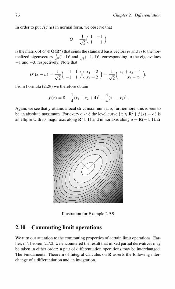
76 Chapter 2. Differentiation
In order to put H f (a) in normal form, we observe that
O = 1√2
( 1 −11 1
)is the matrix of O ∈ O(Rn) that sends the standard basis vectors e1 and e2 to the nor-malized eigenvectors 1√
2(1, 1)t and 1√
2(−1, 1)t , corresponding to the eigenvalues
−1 and −3, respectively. Note that
Ot(x − a) = 1√2
( 1 1−1 1
)( x1 + 2x2 + 2
)= 1√
2
( x1 + x2 + 4x2 − x1
).
From Formula (2.29) we therefore obtain
f (x) = 8− 1
4(x1 + x2 + 4)2 − 3
4(x1 − x2)
2.
Again, we see that f attains a local strict maximum at a; furthermore, this is seen tobe an absolute maximum. For every c < 8 the level curve { x ∈ R2 | f (x) = c } isan ellipse with its major axis along R(1, 1) and minor axis along a + R(−1, 1).✰
Illustration for Example 2.9.9
2.10 Commuting limit operations
We turn our attention to the commuting properties of certain limit operations. Ear-lier, in Theorem 2.7.2, we encountered the result that mixed partial derivatives maybe taken in either order: a pair of differentiation operations may be interchanged.The Fundamental Theorem of Integral Calculus on R asserts the following inter-change of a differentiation and an integration.
2.10. Commuting limit operations 77
Theorem 2.10.1 (Fundamental Theorem of Integral Calculus on R). Let I =[ a, b ] and assume f : I → R is continuous. If f ′ : I → R is also continuousthen
d
dx
∫ x
af (ξ) dξ = f (x) = f (a)+
∫ x
af ′(ξ) dξ (x ∈ I ).
We recall that the first identity, which may be established using estimates, isthe essential one. The second identity then follows from the fact that both f andx �→ ∫ x
a f ′(ξ) dξ have the same derivative.The theorem is of great importance in this section, where we study the differ-
entiability or integrability of integrals depending on a parameter. As a first step weconsider the continuity of such integrals.
Theorem 2.10.2 (Continuity Theorem). Suppose K is a compact subset of Rn
and J = [ c, d ] a compact interval in R. Let f : K × J → Rp be a continuousmapping. Then the mapping F : K → Rp, given by
F(x) =∫
Jf (x, t) dt,
is continuous. Here the integration is by components. In particular we obtain, fora ∈ K ,
limx→a
∫J
f (x, t) dt =∫
Jlimx→a
f (x, t) dt.
Proof. We have, for x and a ∈ K ,
‖F(x)− F(a)‖ =∥∥∥ ∫
J( f (x, t)− f (a, t)) dt
∥∥∥ ≤ ∫J‖ f (x, t)− f (a, t)‖ dt.
On account of Theorem 1.8.15 the mapping f is uniformly continuous on thecompact subset K × J of Rn ×R. Hence, given any ε > 0 we can find δ > 0 suchthat
‖ f (x, t)− f (a, t0)‖ < ε
d − cif ‖(x, t)− (a, t0)‖ < δ.
In particular, we obtain this estimate for f if ‖x − a‖ < δ and t = t0. Therefore,for such x and a
‖F(x)− F(a)‖ ≤∫
J
ε
d − cdt = ε.
This proves the continuity of F at every a ∈ K . ❏
Example 2.10.3. Let f (x, t) = cos xt . Then the conditions of the theorem aresatisfied for every compact set K ⊂ R and J = [ 0, 1 ]. In particular, for x varyingin compacta containing 0,
F(x) =∫ 1
0cos xt dt =
sin x
x, x = 0;
1, x = 0.
Accordingly, the continuity of F at 0 yields the well-known limit limx→0sin x
x = 1.✰
78 Chapter 2. Differentiation
Theorem 2.10.4 (Differentiation Theorem). Suppose K is a compact subset ofRn with nonempty interior U and J = [ c, d ] a compact interval in R. Let f :K × J → Rp be a mapping with the following properties:
(i) f is continuous;
(ii) the total derivative D1 f : U× J → Lin(Rn,Rp)with respect to the variablein U is continuous.
Then F : U → Rp, given by F(x) = ∫J f (x, t) dt, is a differentiable mapping
satisfying
D∫
Jf (x, t) dt =
∫J
D1 f (x, t) dt (x ∈ U ).
Proof. Let a ∈ U and suppose h ∈ Rn is sufficiently small. The derivative of themapping: R → Rp with s �→ f (a + sh, t) is given by s �→ D1 f (a + sh, t) h;hence we have, according to the Fundamental Theorem 2.10.1,
f (a + h, t)− f (a, t) =∫ 1
0D1 f (a + sh, t) ds h.
Furthermore, the right–hand side depends continuously on t ∈ J . Therefore
F(a + h)− F(a) =∫
J( f (a + h, t)− f (a, t)) dt
=∫
J
∫ 1
0D1 f (a + sh, t) ds dt h =: φ(a + h)h,
where φ : U → Lin(Rn,Rp). Applying the Continuity Theorem 2.10.2 twice weobtain
limh→0
φ(a + h) =∫
J
∫ 1
0limh→0
D1 f (a + sh, t) ds dt =∫
JD1 f (a, t) dt = φ(a).
On the strength of Hadamard’s Lemma 2.2.7 this implies the differentiability of Fat a, with derivative
∫J D1 f (a, t) dt . ❏
Example 2.10.5. If we use the Differentiation Theorem 2.10.4 for computing F ′and F ′′ where F denotes the function from Example 2.10.3, we obtain∫ 1
0t sin xt dt = 1
x2(sin x − x cos x),
∫ 1
0t2 cos xt dt = 1
x3((x2 − 2) sin x + 2x cos x).
Application of the Continuity Theorem 2.10.2 now gives
limx→0
1
x3((x2 − 2) sin x + 2x cos x) = 1
3. ✰
2.10. Commuting limit operations 79
Example 2.10.6. Let a > 0 and define f : [ 0, a ] × [ 0, 1 ] → R by
f (x, t) =
arctan
t
x, 0 < x ≤ a;
π
2, x = 0.
Then f is bounded everywhere but discontinuous at (0, 0) and D1 f (x, t) = − tx2+t2 ,
which implies that D1 f is unbounded on [ 0, a ]× [ 0, 1 ] near (0, 0). Therefore theconclusions of the Theorems 2.10.2 and 2.10.4 above do not follow automaticallyin this case. Indeed, F(x) = ∫ 1
0 f (x, t) dt is given by F(0) = π2 and
F(x) =∫ 1
0arctan
t
xdt = arctan
1
x+ 1
2x log
x2
1+ x2(x ∈ R+).
We see that F is continuous at 0 but that F is not differentiable at 0 (use Exercise 0.3if necessary). Still, one can compute that F ′(x) = 1
2 log x2
1+x2 , for all x ∈ R+, whichmay be done in two different ways.
Similar problems arise with G : [ 0,∞ [ → R given by G(0) = −2 and
G(x) =∫ 1
0log(x2 + t2) dt = log(1+ x2)− 2+ 2x arctan
1
x(x ∈ R+).
Then G ′(x) = 2 arctan 1x , thus limx↓0 G ′(x) = π while the partial derivative of the
integrand with respect to x vanishes for x = 0. ✰
In the Differentiation Theorem 2.10.4 we considered the operations of differ-entiation with respect to a variable x and integration with respect to a variable t ,and we showed that under suitable conditions these commute. There are also theoperations of differentiation with respect to t and integration with respect to x . Thefollowing theorem states the remarkable result that the commutativity of any pairof these operations associated with distinct variables implies the commutativity ofthe other two pairs.
Theorem 2.10.7. Let I = [ a, b ] and J = [ c, d ] be intervals in R. Then thefollowing assertions are equivalent.
(i) Let f and D1 f be continuous on I × J . Then x �→∫
Jf (x, y) dy is differ-
entiable, and
D∫
Jf (x, y) dy =
∫J
D1 f (x, y) dy (x ∈ int(I )).
(ii) Let f , D2 f and D1 D2 f be continuous on I × J and assume D1 f (x, c) existsfor x ∈ I . Then D1 f and D2 D1 f exist on the interior of I × J , and on thatinterior
D1 D2 f = D2 D1 f.
80 Chapter 2. Differentiation
(iii) (Interchanging the order of integration). Let f be continuous on I × J .
Then the functions x �→∫
Jf (x, y) dy and y �→
∫I
f (x, y) dx are continu-
ous, and ∫I
∫J
f (x, y) dy dx =∫
J
∫I
f (x, y) dx dy.
Furthermore, all three of these statements are valid.
Proof. For 1 ≤ i ≤ 2, we define Ii and Ei acting on C(I × J ) by
I1 f (x, y) =∫ x
af (ξ, y) dξ, I2 f (x, y) =
∫ y
cf (x, η) dη;
E1 f (x, y) = f (a, y), E2 f (x, y) = f (x, c).
The following identities (1) and (2) (where well-defined) are mere reformulationsof the Fundamental Theorem 2.10.1, while the remaining ones are straightforward,for 1 ≤ i ≤ 2,
(1) Di Ii = I, (2) Ii Di = I − Ei ,
(3) Di Ei = 0, (4) Ei Ii = 0,
(5) D j Ei = Ei D j ( j = i), (6) I j Ei = Ei I j ( j = i).
Now we are prepared for the proof of the equivalence; in this proof we write ‘ass’for ‘assumption’.(i)⇒ (ii), that is, D1 I2 = I2 D1 implies D1 D2 = D2 D1.We have
D1 =(2)
D1 I2 D2 + D1 E2 =ass
I2 D1 D2 + D1 E2.
This shows that D1 f exists. Furthermore, D1 f is differentiable with respect to yand
D2 D1 =(5)
D2 I2 D1 D2 + D2 E2 D1 =(1)+(3)
D1 D2.
(ii)⇒ (iii), that is, D1 D2 = D2 D1 implies I1 I2 = I2 I1.The continuity of the integrals follows from Theorem 2.10.2. Using (1) we seethat I2 I1 f satisfies the conditions imposed on f in (ii) (note that I2 I1 f (x, c) = 0).Therefore
I1 I2 =(1)
I1 I2 D1 I1 =(1)
I1 I2 D1 D2 I2 I1 =ass
I1 I2 D2 D1 I2 I1 =(2)
I1 D1 I2 I1 − I1 E2 D1 I2 I1
=(2)+(5)
I2 I1 − E1 I2 I1 − I1 D1 E2 I2 I1 =(6)+(4)
I2 I1 − I2 E1 I1 =(4)
I2 I1.
(iii)⇒ (i), that is, I1 I2 = I2 I1 implies D1 I2 = I2 D1.Observe that D1 f satisfies the conditions imposed on f in (iii), hence
D1 I2 =(2)
D1 I2 I1 D1 + D1 I2 E1 =ass+(6)
D1 I1 I2 D1 + D1 E1 I2 =(1)+(3)
I2 D1.
2.10. Commuting limit operations 81
Apply this identity to f and evaluate at y = d.The Differentiation Theorem 2.10.4 implies the validity of assertion (i), and
therefore the assertions (ii) and (iii) also hold. ❏
In assertion (ii) the condition on D1 f (x, c) is necessary for the following reason.If f (x, y) = g(x), then D2 f and D1 D2 f both equal 0, but D1 f exists only if g isdifferentiable. Note that assertion (ii) is a stronger form of Theorem 2.7.2, as theconditions in (ii) are weaker.
In Corollary 6.4.3 we will give a different proof for assertion (iii) that is basedon the theory of Riemann integration.
In more intuitive terms the assertions in the theorem above can be put as follows.
(i) A person slices a cake from west to east; then the rate of change of the areaof a cake slice equals the average over the slice of the rate of change of theheight of the cake.
(ii) A person walks on a hillside and points a flashlight along a tangent to thehill; then the rate at which the beam’s slope changes when walking north andpointing east equals its rate of change when walking east and pointing north.
(iii) A person gets just as much cake to eat if he slices it from west to east or fromsouth to north.
Example 2.10.8 (Frullani’s integral). Let 0 < a < b and define f : [ 0, 1 ] ×[ a, b ] by f (x, y) = x y . Then f is continuous and satisfies∫ 1
0
∫ b
af (x, y) dy dx =
∫ 1
0
∫ b
aey log x dy dx =
∫ 1
0
xb − xa
log xdx .
On the other hand,∫ b
a
∫ 1
0f (x, y) dx dy =
∫ b
a
1
y + 1dy = log
b + 1
a + 1.
Theorem 2.10.7.(iii) now implies∫ 1
0
xb − xa
log xdx = log
b + 1
a + 1.
Using the substitution x = e−t one deduces Frullani’s integral∫R+
e−at − e−bt
tdt = log
b
a. ✰
Define f : R2 → R by f (x, t) = xe−xt . Then f is continuous and theimproper integral F(x) = ∫
R+ f (x, t) dt exists, for every x ≥ 0. Nevertheless,F : [ 0,∞ [ → R is discontinuous, since it only assumes the values 0, at 0,
82 Chapter 2. Differentiation
and 1, elsewhere on R+. Without extra conditions the Continuity Theorem 2.10.2apparently is not valid for improper integrals. In order to clarify the situationconsider the rate of convergence of the improper integral. In fact, for d ∈ R+ andx ∈ R+ we have
1−∫ d
0xe−xt dt = e−xd,
and this only tends to 0 if xd tends to ∞. Hence the convergence becomes slowerand slower for x approaching 0. The purpose of the next definition is to rule outthis sort of behavior.
Definition 2.10.9. Suppose A is a subset of Rn and J = [ c,∞ [ an unboundedinterval in R. Let f : A×J → Rp be a continuous mapping and define F : A → Rp
by F(x) = ∫J f (x, t) dt . We say that
∫J f (x, t) dt is uniformly convergent for
x ∈ A if for every ε > 0 there exists D > c such that
x ∈ A and d ≥ D =⇒∥∥∥F(x)−
∫ d
cf (x, t) dt
∥∥∥ < ε. ❍
The following lemma gives a useful criterion for uniform convergence; its proofis straightforward.
Lemma 2.10.10 (De la Vallée-Poussin’s test). Suppose A is a subset of Rn andJ = [ c,∞ [ an unbounded interval in R. Let f : A × J → Rp be a continuousmapping. Suppose there exists a function g : J → [ 0,∞ [ such that ‖ f (x, t)‖ ≤g(t), for all (x, t) ∈ A × J , and
∫J g(t) dt is convergent. Then
∫J f (x, t) dt is
uniformly convergent for x ∈ A.
The test above is only applicable to integrands that are absolutely convergent.In the case of conditional convergence of an integral one might try to transform itinto an absolutely convergent integral through integration by parts.
Example 2.10.11. For every 0 < p ≤ 1, we prove the uniform convergence forx ∈ I := [ 0,∞ [ of
Fp(x) :=∫
R+f p(x, t) dt :=
∫R+
e−xt sin t
t pdt.
Note that the integrand is continuous at 0, hence our concern here is its behavior at∞. To this end, observe that
∫e−xt sin t dt = − e−xt
1+x2 (cos t + x sin t) =: g(x, t). Inparticular, for all (x, t) ∈ I × I ,
|g(x, t)| ≤ 1+ x
1+ x2≤ 2+ 2x2
1+ x2= 2.
2.10. Commuting limit operations 83
Integration by parts now yields, for all d < d ′ ∈ R+,∫ d ′
de−xt sin t
t pdt =
[1
t pg(x, t)
]d ′
d
+ p∫ d ′
d
1
t p+1g(x, t) dt.
For d ′ → ∞, the boundary term converges and the second integral is absolutelyconvergent. Therefore Fp(x) converges, even for x = 0. Furthermore, the uniformconvergence now follows from the estimate, valid for all x ∈ I and d ∈ R+,∣∣∣ ∫ ∞
de−xt sin t
t pdt
∣∣∣ ≤ 2
d p+ 2p
∫ ∞
d
1
t p+1dt = 4
d p.
Note that, in particular, we have proved the convergence of∫R+
sin t
t pdt (0 < p ≤ 1).
Nevertheless, this convergence is only conditional. Indeed,∫
R+sin t
t dt is not abso-lutely convergent as follows from∫
R+
| sin t |t
dt =∑k∈N0
∫ (k+1)π
kπ
| sin t |t
dt =∑k∈N0
∫ π
0
sin t
t + kπdt
≥∑k∈N0
1
(k + 1)π
∫ π
0sin t dt.
✰
Theorem 2.10.12 (Continuity Theorem). Suppose K is a compact subset of Rn
and J = [ c,∞ [ an unbounded interval in R. Let f : K× J → Rp be a continuousmapping. Suppose that the mapping F : K → Rp given by F(x) = ∫
J f (x, t) dtis well-defined and that the integral converges uniformly for x ∈ K . Then F iscontinuous. In particular we obtain, for a ∈ K ,
limx→a
∫J
f (x, t) dt =∫
Jlimx→a
f (x, t) dt.
Proof. Let ε > 0 be arbitrary and select d > c such that, for every x ∈ K ,∥∥∥F(x)−∫ d
cf (x, t) dt
∥∥∥ < ε
3.
Now apply Theorem 2.10.2 with f : K × [ c, d ] → Rp and a ∈ K . This gives theexistence of δ > 0 such that we have, for all x ∈ K with ‖x − a‖ < δ,
� :=∥∥∥ ∫ d
cf (x, t) dt −
∫ d
cf (a, t) dt
∥∥∥ < ε
3.
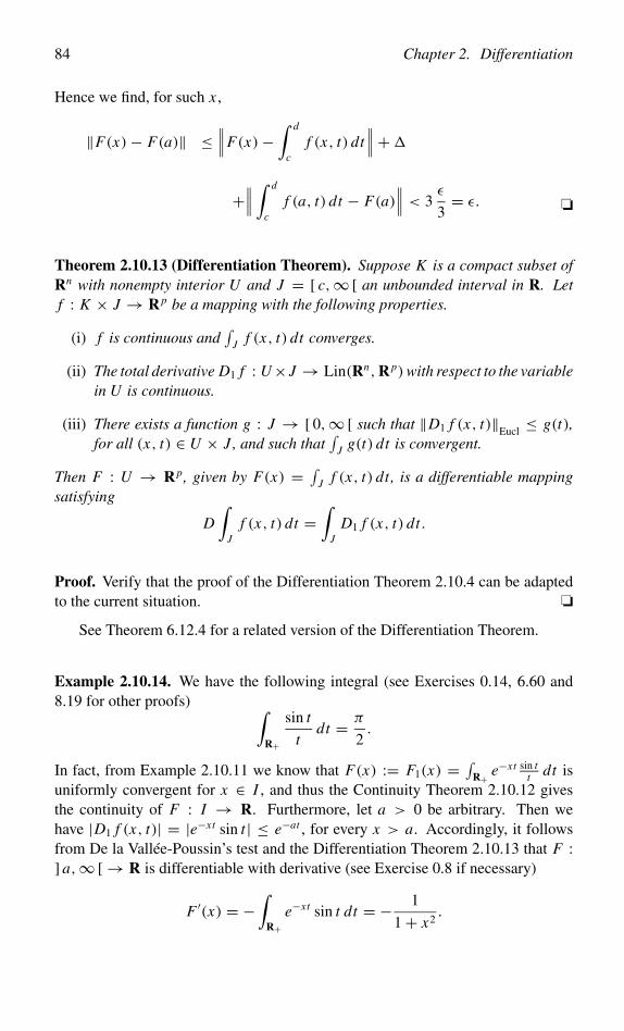
84 Chapter 2. Differentiation
Hence we find, for such x ,
‖F(x)− F(a)‖ ≤∥∥∥F(x)−
∫ d
cf (x, t) dt
∥∥∥+�
+∥∥∥ ∫ d
cf (a, t) dt − F(a)
∥∥∥ < 3ε
3= ε. ❏
Theorem 2.10.13 (Differentiation Theorem). Suppose K is a compact subset ofRn with nonempty interior U and J = [ c,∞ [ an unbounded interval in R. Letf : K × J → Rp be a mapping with the following properties.
(i) f is continuous and∫
J f (x, t) dt converges.
(ii) The total derivative D1 f : U× J → Lin(Rn,Rp)with respect to the variablein U is continuous.
(iii) There exists a function g : J → [ 0,∞ [ such that ‖D1 f (x, t)‖Eucl ≤ g(t),for all (x, t) ∈ U × J , and such that
∫J g(t) dt is convergent.
Then F : U → Rp, given by F(x) = ∫J f (x, t) dt, is a differentiable mapping
satisfying
D∫
Jf (x, t) dt =
∫J
D1 f (x, t) dt.
Proof. Verify that the proof of the Differentiation Theorem 2.10.4 can be adaptedto the current situation. ❏
See Theorem 6.12.4 for a related version of the Differentiation Theorem.
Example 2.10.14. We have the following integral (see Exercises 0.14, 6.60 and8.19 for other proofs) ∫
R+
sin t
tdt = π
2.
In fact, from Example 2.10.11 we know that F(x) := F1(x) =∫
R+ e−xt sin tt dt is
uniformly convergent for x ∈ I , and thus the Continuity Theorem 2.10.12 givesthe continuity of F : I → R. Furthermore, let a > 0 be arbitrary. Then wehave |D1 f (x, t)| = |e−xt sin t | ≤ e−at , for every x > a. Accordingly, it followsfrom De la Vallée-Poussin’s test and the Differentiation Theorem 2.10.13 that F :] a,∞ [ → R is differentiable with derivative (see Exercise 0.8 if necessary)
F ′(x) = −∫
R+e−xt sin t dt = − 1
1+ x2.
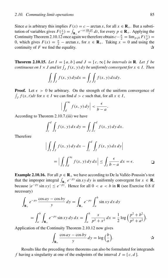
2.10. Commuting limit operations 85
Since a is arbitrary this implies F(x) = c − arctan x , for all x ∈ R+. But a substi-tution of variables gives F( x
p ) =∫
R+ e−xt sin ptt dt , for every p ∈ R+. Applying the
Continuity Theorem 2.10.12 once again we therefore obtain c− π2 = lim p↓0 F( x
p ) =0, which gives F(x) = π
2 − arctan x , for x ∈ R+. Taking x = 0 and using thecontinuity of F we find the equality. ✰
Theorem 2.10.15. Let I = [ a, b ] and J = [ c,∞ [ be intervals in R. Let f becontinuous on I × J and let
∫J f (x, y) dy be uniformly convergent for x ∈ I . Then∫
I
∫J
f (x, y) dydx =∫
J
∫I
f (x, y) dxdy.
Proof. Let ε > 0 be arbitrary. On the strength of the uniform convergence of∫J f (x, t)dt for x ∈ I we can find d > c such that, for all x ∈ I ,∣∣∣ ∫ ∞
df (x, y) dy
∣∣∣ < ε
b − a.
According to Theorem 2.10.7.(iii) we have∫ d
c
∫I
f (x, y) dx dy =∫
I
∫ d
cf (x, y) dy dx .
Therefore ∣∣∣ ∫I
∫J
f (x, y) dy dx −∫ d
c
∫I
f (x, y) dx dy∣∣∣
=∣∣∣ ∫
I
∫ ∞
df (x, y) dy dx
∣∣∣ ≤ ∫I
ε
b − adx = ε. ❏
Example 2.10.16. For all p ∈ R+ we have according to De la Vallée-Poussin’s testthat the improper integral
∫R+ e−py sin xy dy is uniformly convergent for x ∈ R,
because |e−py sin xy| ≤ e−py . Hence for all 0 < a < b in R (see Exercise 0.8 ifnecessary)∫
R+e−py cos ay − cos by
ydy =
∫R+
e−py∫ b
asin xy dx dy
=∫ b
a
∫R+
e−py sin xy dy dx =∫ b
a
x
p2 + x2dx = 1
2log
( p2 + b2
p2 + a2
).
Application of the Continuity Theorem 2.10.12 now gives∫R+
cos ay − cos by
ydy = log
(b
a
). ✰
Results like the preceding three theorems can also be formulated for integrandsf having a singularity at one of the endpoints of the interval J = [ c, d ].

Chapter 3
Inverse Function and ImplicitFunction Theorems
The main theme in this chapter is that the local behavior of a differentiable mapping,near a point, is qualitatively determined by that of its derivative at the point inquestion. Diffeomorphisms are differentiable substitutions of variables appearing,for example, in the description of geometrical objects in Chapter 4 and in the Changeof Variables Theorem in Chapter 6. Useful criteria, in terms of derivatives, fordeciding whether a mapping is a diffeomorphism are given in the Inverse FunctionTheorems. Next comes the Implicit Function Theorem, which is a fundamentalresult concerning existence and uniqueness of solutions for a system of n equationsin n unknowns in the presence of parameters. The theorem will be applied inthe study of geometrical objects; it also plays an important part in the Change ofVariables Theorem for integrals.
3.1 Diffeomorphisms
A suitable change of variables, or diffeomorphism (this term is a contraction ofdifferentiable and homeomorphism), can sometimes solve a problem that looksintractable otherwise. Changes of variables, which were already encountered in theintegral calculus on R, will reappear later in the Change of Variables Theorem 6.6.1.
Example 3.1.1 (Polar coordinates). (See also Example 6.6.4.) Let
V = { (r, α) ∈ R2 | r ∈ R+, −π < α < π },and let
U = R2 \ { (x1, 0) ∈ R2 | x1 ≤ 0 }
87
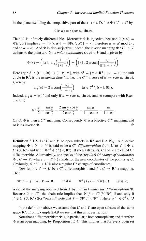
88 Chapter 3. Inverse and Implicit Function Theorems
be the plane excluding the nonpositive part of the x1-axis. Define � : V → U by
�(r, α) = r (cosα, sin α).
Then � is infinitely differentiable. Moreover � is injective, because �(r, α) =�(r ′, α′) implies r = ‖�(r, α)‖ = ‖�(r ′, α′)‖ = r ′; therefore α ≡ α′ mod 2π ,and so α = α′. And � is also surjective; indeed, the inverse mapping � : U → Vassigns to the point x ∈ U its polar coordinates (r, α) ∈ V and is given by
�(x) =(‖x‖, arg
( 1
‖x‖ x))=
(‖x‖, 2 arctan
( x2
‖x‖ + x1
)).
Here arg : S1 \ {(−1, 0)} → ]−π, π [, with S1 = { u ∈ R2 | ‖u‖ = 1 } the unitcircle in R2, is the argument function, i.e. the C∞ inverse of α �→ (cosα, sin α),given by
arg(u) = 2 arctan( u2
1+ u1
)(u ∈ S1 \ {(−1, 0)}).
Indeed, arg u = α if and only if u = (cosα, sin α), and so (compare with Exer-cise 0.1)
tanα
2= sin α
2
cos α2
= 2 sin α2 cos α
2
2 cos2 α2
= sin α
1+ cosα= u2
1+ u1.
On U , � is then a C∞ mapping. Consequently � is a bijective C∞ mapping, andso is its inverse �. ✰
Definition 3.1.2. Let U and V be open subsets in Rn and k ∈ N∞. A bijectivemapping � : U → V is said to be a Ck diffeomorphism from U to V if � ∈Ck(U,Rn) and � := �−1 ∈ Ck(V,Rn). If such a � exists, U and V are called Ck
diffeomorphic. Alternatively, one speaks of the (regular) Ck change of coordinates� : U → V , where y = �(x) stands for the new coordinates of the point x ∈ U .Obviously, � : V → U is also a regular Ck change of coordinates.
Now let � : V → U be a Ck diffeomorphism and f : U → Rp a mapping.Then
�∗ f = f ◦� : V → R, that is �∗ f (y) = f (�(y)) (y ∈ V ),
is called the mapping obtained from f by pullback under the diffeomorphism �.Because � ∈ Ck , the chain rule implies that �∗ f ∈ Ck(V,Rp) if and only iff ∈ Ck(U,Rp) (for “only if”, note that f = (�∗ f ) ◦�−1, where �−1 ∈ Ck). ❍
In the definition above we assume that U and V are open subsets of the samespace Rn . From Example 2.4.9 we see that this is no restriction.
Note that a diffeomorphism� is, in particular, a homeomorphism; and therefore� is an open mapping, by Proposition 1.5.4. This implies that for every open set
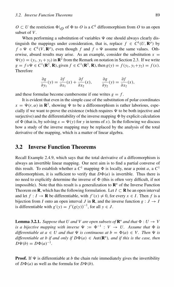
3.2. Inverse Function Theorems 89
O ⊂ U the restriction �|O of � to O is a Ck diffeomorphism from O to an opensubset of V .
When performing a substitution of variables � one should always clearly dis-tinguish the mappings under consideration, that is, replace f ∈ Ck(U,Rp) byf ◦ � ∈ Ck(V,Rp), even though f and f ◦ � assume the same values. Oth-erwise, absurd results may arise. As an example, consider the substitution x =�(y) = (y1, y1+ y2) in R2 from the Remark on notation in Section 2.3. If we writeg = f ◦� ∈ C1(R2,R), given f ∈ C1(R2,R), then g(y) = f (y1, y1+y2) = f (x).Therefore
∂g
∂y1(y) = ∂ f
∂x1(x)+ ∂ f
∂x2(x),
∂g
∂y2(y) = ∂ f
∂x2(x),
and these formulae become cumbersome if one writes g = f .It is evident that even in the simple case of the substitution of polar coordinates
x = �(r, α) in R2, showing � to be a diffeomorphism is rather laborious, espe-cially if we want to prove the existence (which requires � to be both injective andsurjective) and the differentiability of the inverse mapping� by explicit calculationof � (that is, by solving x = �(y) for y in terms of x). In the following we discusshow a study of the inverse mapping may be replaced by the analysis of the totalderivative of the mapping, which is a matter of linear algebra.
3.2 Inverse Function Theorems
Recall Example 2.4.9, which says that the total derivative of a diffeomorphism isalways an invertible linear mapping. Our next aim is to find a partial converse ofthis result. To establish whether a C1 mapping � is locally, near a point a, a C1
diffeomorphism, it is sufficient to verify that D�(a) is invertible. Thus there isno need to explicitly determine the inverse of � (this is often very difficult, if notimpossible). Note that this result is a generalization to Rn of the Inverse FunctionTheorem on R, which has the following formulation. Let I ⊂ R be an open intervaland let f : I → R be differentiable, with f ′(x) = 0, for every x ∈ I . Then f is abijection from I onto an open interval J in R, and the inverse function g : J → Iis differentiable with g′(y) = f ′(g(y))−1, for all y ∈ J .
Lemma 3.2.1. Suppose that U and V are open subsets of Rn and that � : U → Vis a bijective mapping with inverse � := �−1 : V → U. Assume that � isdifferentiable at a ∈ U and that � is continuous at b = �(a) ∈ V . Then � isdifferentiable at b if and only if D�(a) ∈ Aut(Rn), and if this is the case, thenD�(b) = D�(a)−1.
Proof. If � is differentiable at b the chain rule immediately gives the invertibilityof D�(a) as well as the formula for D�(b).
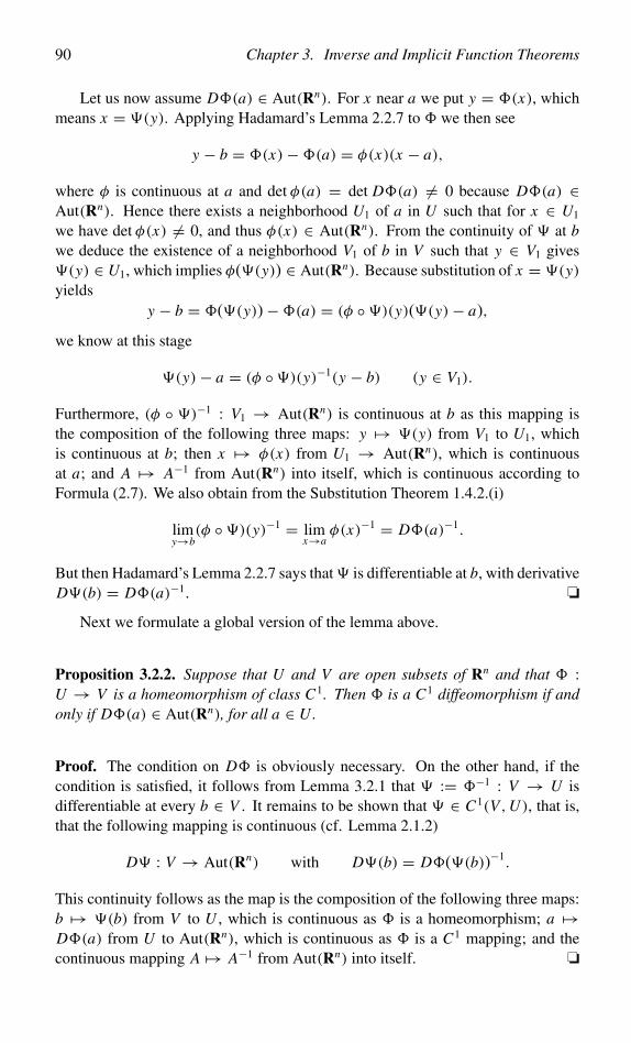
90 Chapter 3. Inverse and Implicit Function Theorems
Let us now assume D�(a) ∈ Aut(Rn). For x near a we put y = �(x), whichmeans x = �(y). Applying Hadamard’s Lemma 2.2.7 to � we then see
y − b = �(x)−�(a) = φ(x)(x − a),
where φ is continuous at a and det φ(a) = det D�(a) = 0 because D�(a) ∈Aut(Rn). Hence there exists a neighborhood U1 of a in U such that for x ∈ U1
we have det φ(x) = 0, and thus φ(x) ∈ Aut(Rn). From the continuity of � at bwe deduce the existence of a neighborhood V1 of b in V such that y ∈ V1 gives�(y) ∈ U1, which implies φ(�(y)) ∈ Aut(Rn). Because substitution of x = �(y)yields
y − b = �(�(y))−�(a) = (φ ◦�)(y)(�(y)− a),
we know at this stage
�(y)− a = (φ ◦�)(y)−1(y − b) (y ∈ V1).
Furthermore, (φ ◦ �)−1 : V1 → Aut(Rn) is continuous at b as this mapping isthe composition of the following three maps: y �→ �(y) from V1 to U1, whichis continuous at b; then x �→ φ(x) from U1 → Aut(Rn), which is continuousat a; and A �→ A−1 from Aut(Rn) into itself, which is continuous according toFormula (2.7). We also obtain from the Substitution Theorem 1.4.2.(i)
limy→b
(φ ◦�)(y)−1 = limx→a
φ(x)−1 = D�(a)−1.
But then Hadamard’s Lemma 2.2.7 says that� is differentiable at b, with derivativeD�(b) = D�(a)−1. ❏
Next we formulate a global version of the lemma above.
Proposition 3.2.2. Suppose that U and V are open subsets of Rn and that � :U → V is a homeomorphism of class C1. Then � is a C1 diffeomorphism if andonly if D�(a) ∈ Aut(Rn), for all a ∈ U.
Proof. The condition on D� is obviously necessary. On the other hand, if thecondition is satisfied, it follows from Lemma 3.2.1 that � := �−1 : V → U isdifferentiable at every b ∈ V . It remains to be shown that � ∈ C1(V,U ), that is,that the following mapping is continuous (cf. Lemma 2.1.2)
D� : V → Aut(Rn) with D�(b) = D�(�(b))−1.
This continuity follows as the map is the composition of the following three maps:b �→ �(b) from V to U , which is continuous as � is a homeomorphism; a �→D�(a) from U to Aut(Rn), which is continuous as � is a C1 mapping; and thecontinuous mapping A �→ A−1 from Aut(Rn) into itself. ❏
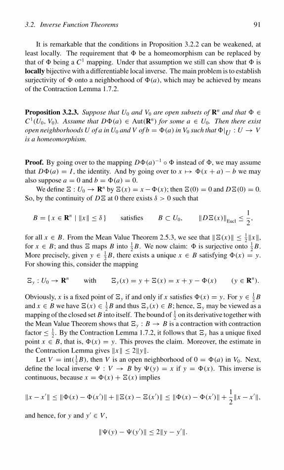
3.2. Inverse Function Theorems 91
It is remarkable that the conditions in Proposition 3.2.2 can be weakened, atleast locally. The requirement that � be a homeomorphism can be replaced bythat of � being a C1 mapping. Under that assumption we still can show that � islocally bijective with a differentiable local inverse. The main problem is to establishsurjectivity of � onto a neighborhood of �(a), which may be achieved by meansof the Contraction Lemma 1.7.2.
Proposition 3.2.3. Suppose that U0 and V0 are open subsets of Rn and that � ∈C1(U0, V0). Assume that D�(a) ∈ Aut(Rn) for some a ∈ U0. Then there existopen neighborhoods U of a in U0 and V of b = �(a) in V0 such that�|U : U → Vis a homeomorphism.
Proof. By going over to the mapping D�(a)−1 ◦� instead of �, we may assumethat D�(a) = I , the identity. And by going over to x �→ �(x + a) − b we mayalso suppose a = 0 and b = �(a) = 0.
We define� : U0 → Rn by�(x) = x−�(x); then�(0) = 0 and D�(0) = 0.So, by the continuity of D� at 0 there exists δ > 0 such that
B = { x ∈ Rn | ‖x‖ ≤ δ } satisfies B ⊂ U0, ‖D�(x)‖Eucl ≤1
2,
for all x ∈ B. From the Mean Value Theorem 2.5.3, we see that ‖�(x)‖ ≤ 12‖x‖,
for x ∈ B; and thus � maps B into 12 B. We now claim: � is surjective onto 1
2 B.More precisely, given y ∈ 1
2 B, there exists a unique x ∈ B satisfying �(x) = y.For showing this, consider the mapping
�y : U0 → Rn with �y(x) = y +�(x) = x + y −�(x) (y ∈ Rn).
Obviously, x is a fixed point of �y if and only if x satisfies �(x) = y. For y ∈ 12 B
and x ∈ B we have�(x) ∈ 12 B and thus�y(x) ∈ B; hence, �y may be viewed as a
mapping of the closed set B into itself. The bound of 12 on its derivative together with
the Mean Value Theorem shows that �y : B → B is a contraction with contractionfactor ≤ 1
2 . By the Contraction Lemma 1.7.2, it follows that �y has a unique fixedpoint x ∈ B, that is, �(x) = y. This proves the claim. Moreover, the estimate inthe Contraction Lemma gives ‖x‖ ≤ 2‖y‖.
Let V = int( 12 B), then V is an open neighborhood of 0 = �(a) in V0. Next,
define the local inverse � : V → B by �(y) = x if y = �(x). This inverse iscontinuous, because x = �(x)+�(x) implies
‖x − x ′‖ ≤ ‖�(x)−�(x ′)‖+ ‖�(x)−�(x ′)‖ ≤ ‖�(x)−�(x ′)‖+ 1
2‖x − x ′‖,
and hence, for y and y′ ∈ V ,
‖�(y)−�(y′)‖ ≤ 2‖y − y′‖.
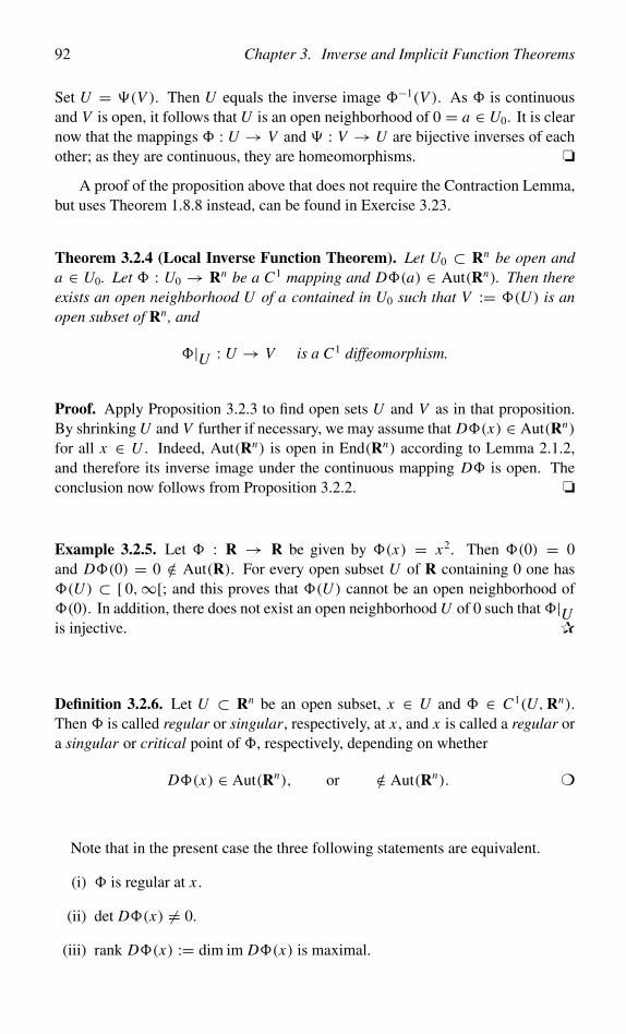
92 Chapter 3. Inverse and Implicit Function Theorems
Set U = �(V ). Then U equals the inverse image �−1(V ). As � is continuousand V is open, it follows that U is an open neighborhood of 0 = a ∈ U0. It is clearnow that the mappings � : U → V and � : V → U are bijective inverses of eachother; as they are continuous, they are homeomorphisms. ❏
A proof of the proposition above that does not require the Contraction Lemma,but uses Theorem 1.8.8 instead, can be found in Exercise 3.23.
Theorem 3.2.4 (Local Inverse Function Theorem). Let U0 ⊂ Rn be open anda ∈ U0. Let � : U0 → Rn be a C1 mapping and D�(a) ∈ Aut(Rn). Then thereexists an open neighborhood U of a contained in U0 such that V := �(U ) is anopen subset of Rn, and
�|U : U → V is a C1 diffeomorphism.
Proof. Apply Proposition 3.2.3 to find open sets U and V as in that proposition.By shrinking U and V further if necessary, we may assume that D�(x) ∈ Aut(Rn)
for all x ∈ U . Indeed, Aut(Rn) is open in End(Rn) according to Lemma 2.1.2,and therefore its inverse image under the continuous mapping D� is open. Theconclusion now follows from Proposition 3.2.2. ❏
Example 3.2.5. Let � : R → R be given by �(x) = x2. Then �(0) = 0and D�(0) = 0 /∈ Aut(R). For every open subset U of R containing 0 one has�(U ) ⊂ [ 0,∞[; and this proves that �(U ) cannot be an open neighborhood of�(0). In addition, there does not exist an open neighborhood U of 0 such that �|Uis injective. ✰
Definition 3.2.6. Let U ⊂ Rn be an open subset, x ∈ U and � ∈ C1(U,Rn).Then � is called regular or singular, respectively, at x , and x is called a regular ora singular or critical point of �, respectively, depending on whether
D�(x) ∈ Aut(Rn), or /∈ Aut(Rn). ❍
Note that in the present case the three following statements are equivalent.
(i) � is regular at x .
(ii) det D�(x) = 0.
(iii) rank D�(x) := dim im D�(x) is maximal.
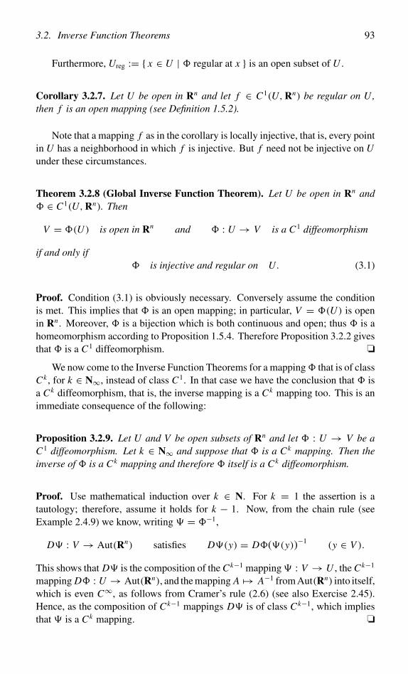
3.2. Inverse Function Theorems 93
Furthermore, Ureg := { x ∈ U | � regular at x } is an open subset of U .
Corollary 3.2.7. Let U be open in Rn and let f ∈ C1(U,Rn) be regular on U,then f is an open mapping (see Definition 1.5.2).
Note that a mapping f as in the corollary is locally injective, that is, every pointin U has a neighborhood in which f is injective. But f need not be injective on Uunder these circumstances.
Theorem 3.2.8 (Global Inverse Function Theorem). Let U be open in Rn and� ∈ C1(U,Rn). Then
V = �(U ) is open in Rn and � : U → V is a C1 diffeomorphism
if and only if� is injective and regular on U. (3.1)
Proof. Condition (3.1) is obviously necessary. Conversely assume the conditionis met. This implies that � is an open mapping; in particular, V = �(U ) is openin Rn . Moreover, � is a bijection which is both continuous and open; thus � is ahomeomorphism according to Proposition 1.5.4. Therefore Proposition 3.2.2 givesthat � is a C1 diffeomorphism. ❏
We now come to the Inverse Function Theorems for a mapping� that is of classCk , for k ∈ N∞, instead of class C1. In that case we have the conclusion that � isa Ck diffeomorphism, that is, the inverse mapping is a Ck mapping too. This is animmediate consequence of the following:
Proposition 3.2.9. Let U and V be open subsets of Rn and let � : U → V be aC1 diffeomorphism. Let k ∈ N∞ and suppose that � is a Ck mapping. Then theinverse of � is a Ck mapping and therefore � itself is a Ck diffeomorphism.
Proof. Use mathematical induction over k ∈ N. For k = 1 the assertion is atautology; therefore, assume it holds for k − 1. Now, from the chain rule (seeExample 2.4.9) we know, writing � = �−1,
D� : V → Aut(Rn) satisfies D�(y) = D�(�(y))−1(y ∈ V ).
This shows that D� is the composition of the Ck−1 mapping� : V → U , the Ck−1
mapping D� : U → Aut(Rn), and the mapping A �→ A−1 from Aut(Rn) into itself,which is even C∞, as follows from Cramer’s rule (2.6) (see also Exercise 2.45).Hence, as the composition of Ck−1 mappings D� is of class Ck−1, which impliesthat � is a Ck mapping. ❏
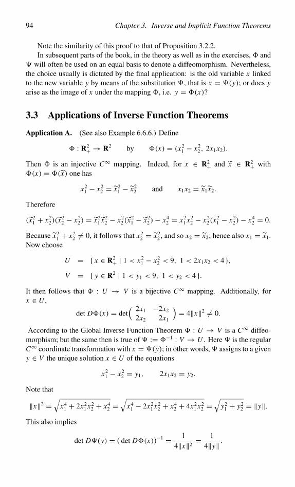
94 Chapter 3. Inverse and Implicit Function Theorems
Note the similarity of this proof to that of Proposition 3.2.2.In subsequent parts of the book, in the theory as well as in the exercises, � and
� will often be used on an equal basis to denote a diffeomorphism. Nevertheless,the choice usually is dictated by the final application: is the old variable x linkedto the new variable y by means of the substitution �, that is x = �(y); or does yarise as the image of x under the mapping �, i.e. y = �(x)?
3.3 Applications of Inverse Function Theorems
Application A. (See also Example 6.6.6.) Define
� : R2+ → R2 by �(x) = (x2
1 − x22 , 2x1x2).
Then � is an injective C∞ mapping. Indeed, for x ∈ R2+ and x ∈ R2+ with�(x) = �(x) one has
x21 − x2
2 = x21 − x2
2 and x1x2 = x1 x2.
Therefore
(x21 + x2
2)(x22 − x2
2) = x21 x2
2 − x22 (x
21 − x2
2)− x42 = x2
1 x22 − x2
2(x21 − x2
2)− x42 = 0.
Because x21 + x2
2 = 0, it follows that x22 = x2
2 , and so x2 = x2; hence also x1 = x1.Now choose
U = { x ∈ R2+ | 1 < x2
1 − x22 < 9, 1 < 2x1x2 < 4 },
V = { y ∈ R2 | 1 < y1 < 9, 1 < y2 < 4 }.It then follows that � : U → V is a bijective C∞ mapping. Additionally, forx ∈ U ,
det D�(x) = det( 2x1 −2x2
2x2 2x1
)= 4‖x‖2 = 0.
According to the Global Inverse Function Theorem � : U → V is a C∞ diffeo-morphism; but the same then is true of � := �−1 : V → U . Here � is the regularC∞ coordinate transformation with x = �(y); in other words, � assigns to a giveny ∈ V the unique solution x ∈ U of the equations
x21 − x2
2 = y1, 2x1x2 = y2.
Note that
‖x‖2 =√
x41 + 2x2
1 x22 + x4
2 =√
x41 − 2x2
1 x22 + x4
2 + 4x21 x2
2 =√
y21 + y2
2 = ‖y‖.This also implies
det D�(y) = ( det D�(x))−1 = 1
4‖x‖2= 1
4‖y‖ .
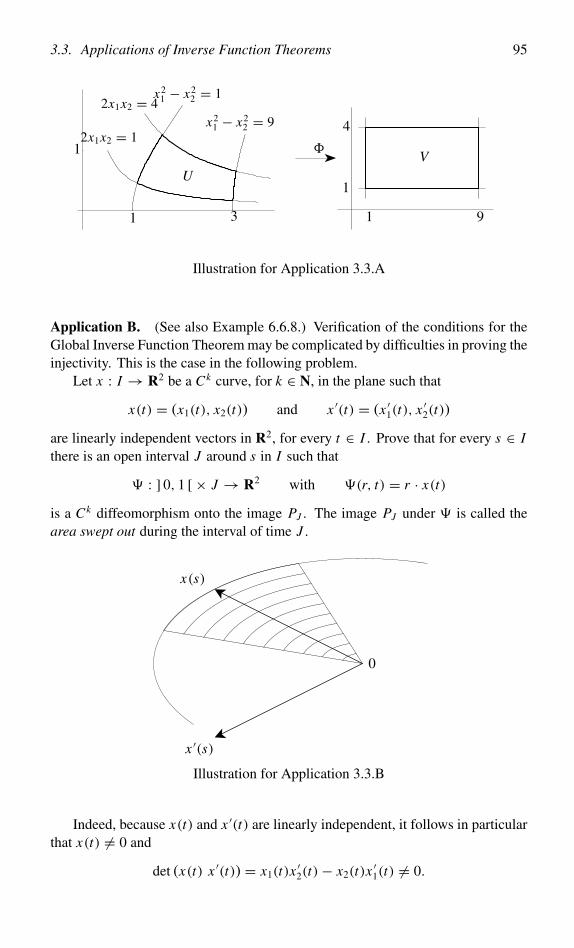
3.3. Applications of Inverse Function Theorems 95
1 9
1
4
�V
U
2x1x2 = 1
2x1x2 = 4x2
1 − x22 = 1
x21 − x2
2 = 9
3 1
1
Illustration for Application 3.3.A
Application B. (See also Example 6.6.8.) Verification of the conditions for theGlobal Inverse Function Theorem may be complicated by difficulties in proving theinjectivity. This is the case in the following problem.
Let x : I → R2 be a Ck curve, for k ∈ N, in the plane such that
x(t) = (x1(t), x2(t)) and x ′(t) = (x ′1(t), x ′2(t))
are linearly independent vectors in R2, for every t ∈ I . Prove that for every s ∈ Ithere is an open interval J around s in I such that
� : ] 0, 1 [× J → R2 with �(r, t) = r · x(t)
is a Ck diffeomorphism onto the image PJ . The image PJ under � is called thearea swept out during the interval of time J .
x(s)
x ′(s)
0
Illustration for Application 3.3.B
Indeed, because x(t) and x ′(t) are linearly independent, it follows in particularthat x(t) = 0 and
det (x(t) x ′(t)) = x1(t)x′2(t)− x2(t)x
′1(t) = 0.
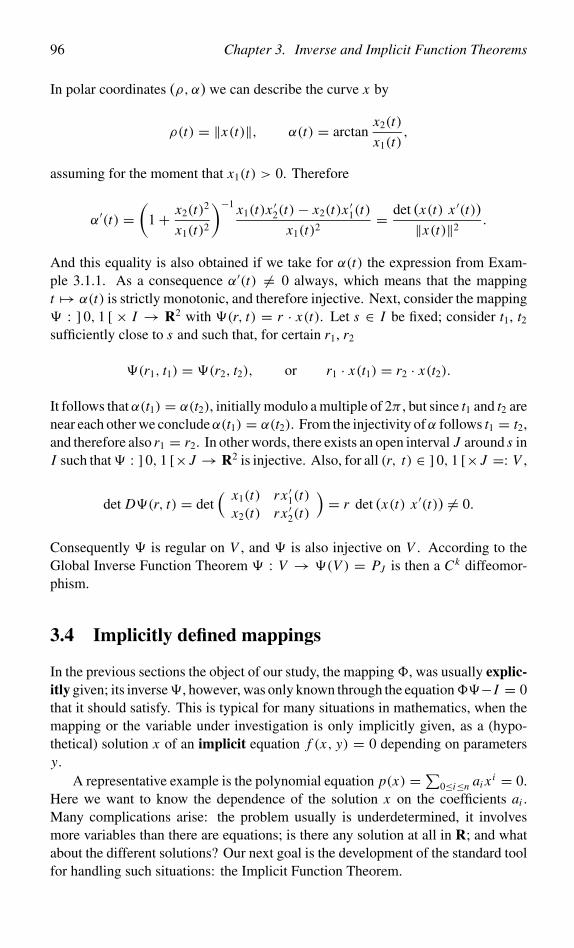
96 Chapter 3. Inverse and Implicit Function Theorems
In polar coordinates (ρ, α) we can describe the curve x by
ρ(t) = ‖x(t)‖, α(t) = arctanx2(t)
x1(t),
assuming for the moment that x1(t) > 0. Therefore
α′(t) =(
1+ x2(t)2
x1(t)2
)−1 x1(t)x ′2(t)− x2(t)x ′1(t)x1(t)2
= det (x(t) x ′(t))‖x(t)‖2
.
And this equality is also obtained if we take for α(t) the expression from Exam-ple 3.1.1. As a consequence α′(t) = 0 always, which means that the mappingt �→ α(t) is strictly monotonic, and therefore injective. Next, consider the mapping� : ] 0, 1 [ × I → R2 with �(r, t) = r · x(t). Let s ∈ I be fixed; consider t1, t2sufficiently close to s and such that, for certain r1, r2
�(r1, t1) = �(r2, t2), or r1 · x(t1) = r2 · x(t2).
It follows that α(t1) = α(t2), initially modulo a multiple of 2π , but since t1 and t2 arenear each other we concludeα(t1) = α(t2). From the injectivity ofα follows t1 = t2,and therefore also r1 = r2. In other words, there exists an open interval J around s inI such that� : ] 0, 1 [× J → R2 is injective. Also, for all (r, t) ∈ ] 0, 1 [× J =: V ,
det D�(r, t) = det( x1(t) r x ′1(t)
x2(t) r x ′2(t)
)= r det (x(t) x ′(t)) = 0.
Consequently � is regular on V , and � is also injective on V . According to theGlobal Inverse Function Theorem � : V → �(V ) = PJ is then a Ck diffeomor-phism.
3.4 Implicitly defined mappings
In the previous sections the object of our study, the mapping �, was usually explic-itly given; its inverse�, however, was only known through the equation��− I = 0that it should satisfy. This is typical for many situations in mathematics, when themapping or the variable under investigation is only implicitly given, as a (hypo-thetical) solution x of an implicit equation f (x, y) = 0 depending on parametersy.
A representative example is the polynomial equation p(x) =∑0≤i≤n ai xi = 0.
Here we want to know the dependence of the solution x on the coefficients ai .Many complications arise: the problem usually is underdetermined, it involvesmore variables than there are equations; is there any solution at all in R; and whatabout the different solutions? Our next goal is the development of the standard toolfor handling such situations: the Implicit Function Theorem.
3.4. Implicitly defined mappings 97
(A) The problem
Consider a system of n equations that depend on p parameters y1, . . . , yp in R, forn unknowns x1, . . . , xn in R:
f1(x1, . . . , xn; y1, . . . , yp) = 0,
......
...
fn(x1, . . . , xn; y1, . . . , yp) = 0.
A condensed notation for this is
f (x; y) = 0, (3.2)
where
f : Rn × Rp ⊃→ Rn, x = (x1, . . . , xn) ∈ Rn, y = (y1, . . . , yp) ∈ Rp.
Assume that for a special value y0 = (y01 , . . . , y0
p) of the parameter there exists asolution x0 = (x0
1 , . . . , x0n) of f (x; y) = 0; i.e.
f (x0; y0) = 0.
It would then be desirable to establish that, for y near y0, there also exists a solutionx near x0 of f (x; y) = 0. If this is the case, we obtain a mapping
ψ : Rp ⊃→ Rn with ψ(y) = x and f (x; y) = 0.
This mapping ψ , which assigns to parameters y near y0 the unique solution x =ψ(y) of f (x; y) = 0, is called the function implicitly defined by f (x; y) = 0. If fdepends on x and y differentiably, one also expectsψ to depend on y differentiably.
The Implicit Function Theorem 3.5.1 decides the validity of these assertions asregards:
• existence,
• uniqueness,
• differentiable dependence on parameters,
of the solutions x = ψ(y) of f (x; y) = 0, for y near y0.
(B) An idea about the solution
Assume f to be a differentiable function of (x, y), and in particular therefore f tobe defined on an open set. From the definition of differentiability:
f (x; y)− f (x0; y0) = D f (x0; y0)( x − x0
y − y0
)+ R(x, y)
= ( Dx f (x0; y0) Dy f (x0; y0) )( x − x0
y − y0
)+ R(x, y)
= Dx f (x0; y0)(x − x0)+ Dy f (x0; y0)(y − y0)+ R(x, y).
(3.3)
98 Chapter 3. Inverse and Implicit Function Theorems
Here
Dx f (x0; y0) ∈ End(Rn), and Dy f (x0; y0) ∈ Lin(Rp,Rn),
denote the derivatives of f with respect to the variable x ∈ Rn , and y ∈ Rp; inJacobi’s notation their matrices with respect to the standard bases are, respectively,
∂ f1
∂x1(x0; y0) · · · ∂ f1
∂xn(x0; y0)
......
∂ fn
∂x1(x0; y0) · · · ∂ fn
∂xn(x0; y0)
,
∂ f1
∂y1(x0; y0) · · · ∂ f1
∂yp(x0; y0)
......
∂ fn
∂y1(x0; y0) · · · ∂ fn
∂yp(x0; y0)
.
For R the usual estimates from Formula (2.10) hold:
lim(x,y)→(x0,y0)
‖R(x, y)‖‖(x − x0, y − y0)‖ = 0,
or alternatively, for every ε > 0 there exists a δ > 0 such that
‖R(x, y)‖ ≤ ε(‖x − x0‖2 + ‖y − y0‖2)1/2,
provided ‖x − x0‖2 + ‖y − y0‖2 < δ2. Therefore, given y near y0, the existenceof a solution x near x0 requires
Dx f (x0; y0)(x − x0)+ Dy f (x0; y0)(y − y0)+ R(x, y) = 0. (3.4)
The Implicit Function Theorem then asserts that a unique solution x = ψ(y) ofEquation (3.4), and therefore of Equation (3.2), exists if the linearized problem
Dx f (x0; y0)(x − x0)+ Dy f (x0; y0)(y − y0) = 0
can be solved for x , in other words if Dx f (x0; y0) ∈ End(Rn) is an invertiblemapping. Or, rephrasing yet again, if
Dx f (x0; y0) ∈ Aut(Rn). (3.5)
(C) Formula for the derivative of the solution
If we now also know thatψ : Rp ⊃→ Rn is differentiable, we have the compositionof differentiable mappings
Rp ⊃→ Rn × Rp → Rn given by yψ×I�−→ (ψ(y), y)
f�→ f (ψ(y), y) = 0.
3.4. Implicitly defined mappings 99
In this case application of the chain rule leads to
D f (ψ(y), y) ◦ D(ψ × I )(y) = 0, (3.6)
or, more explicitly,
( Dx f (ψ(y), y) Dy f (ψ(y), y) )(
Dψ(y)I
)= Dx f (ψ(y), y) Dψ(y)+ Dy f (ψ(y), y) = 0.
In other words, we have the identity of mappings in Lin(Rp,Rn)
Dx f (ψ(y), y) Dψ(y) = −Dy f (ψ(y), y).
Remarkably, under the same condition (3.5) as before we obtain a formula for thederivative Dψ(y0) ∈ Lin(Rp,Rn) at y0 of the implicitly defined function ψ :
Dψ(y0) = −Dx f (ψ(y0); y0)−1 ◦ Dy f (ψ(y0); y0).
(D) The conditions are necessary
To show that problems may arise if condition (3.5) is not met, we consider theequation
f (x; y) = x2 − y = 0.
Let y0 > 0 and let x0 be a solution> 0 (e.g. y0 = 1, x0 = 1). For y > 0 sufficientlyclose to y0, there exists precisely one solution x near x0, and this solution x = √ydepends differentiably on y. Of course, if x0 < 0, then we have the unique solutionx = −√y.
This should be compared with the situation for y0 = 0, with the solution x0 = 0.Note that
Dx f (0; 0) = 2x |x=0 = 0.
For y near y0 = 0 with y > 0 there are two solutions x near x0 = 0 (i.e. x = ±√y),whereas for y near y0 with y < 0 there is no solution x ∈ R. Furthermore, thepositive and negative solutions both depend nondifferentiably on y ≥ 0 at y = y0,since
limy↓0
±√y
y= ±∞.
In addition
limy↓0
ψ ′(y) = limy↓0± 1
2√
y= ±∞.
In other words, the two solutions obtained for positive y collide, their speed increas-ing without bound as y ↓ 0; next, after y has passed through 0 to become negative,they have vanished.
100 Chapter 3. Inverse and Implicit Function Theorems
3.5 Implicit Function Theorem
The proof of the following theorem is by reduction to a situation that can be treatedby means of the Local Inverse Function Theorem. This is done by adding (dummy)equations so that the number of equations equals the number of variables. Foranother proof of the Implicit Function Theorem see Exercise 3.28.
Theorem 3.5.1 (Implicit Function Theorem). Let k ∈ N∞, let W be open inRn × Rp and f ∈ Ck(W,Rn). Assume
(x0, y0) ∈ W, f (x0; y0) = 0, Dx f (x0; y0) ∈ Aut(Rn).
Then there exist open neighborhoods U of x0 in Rn and V of y0 in Rp with thefollowing properties:
for every y ∈ V there exists a unique x ∈ U with f (x; y) = 0.
In this way we obtain a Ck mapping: Rp ⊃→ Rn satisfying
ψ : V → U with ψ(y) = x and f (x; y) = 0,
which is uniquely determined by these properties. Furthermore, the derivativeDψ(y) ∈ Lin(Rp,Rn) of ψ at y is given by
Dψ(y) = −Dx f (ψ(y); y)−1 ◦ Dy f (ψ(y); y) (y ∈ V ).
Proof. Define � ∈ Ck(W,Rn × Rp) by
�(x, y) = ( f (x, y), y).
Then �(x0, y0) = (0, y0), and we have the matrix representation
D�(x, y) =(
Dx f (x, y) Dy f (x, y)
0 I
).
From Dx f (x0, y0) ∈ Aut(Rn)we obtain D�(x0, y0) ∈ Aut(Rn×Rp). Accordingto the Local Inverse Function Theorem 3.2.4 there exist an open neighborhood W0
of (x0, y0) contained in W and an open neighborhood V0 of (0, y0) in Rn×Rp suchthat � : W0 → V0 is a Ck diffeomorphism. Let U and V1 be open neighborhoodsof x0 and y0 in Rn and Rp, respectively, such that U × V1 ⊂ W0. Then � is adiffeomorphism of U × V1 onto an open subset of V0, so that by restriction of �we may assume that U × V1 is W0. Denote by � : V0 → W0 the inverse Ck
diffeomorphism, which is of the form
�(z, y) = (ψ(z, y), y) ((z, y) ∈ V0),
3.6. Applications of the Implicit Function Theorem 101
for a Ck mapping ψ : V0 → Rn . Note that we have the equivalence
(x, y) ∈ W0 and f (x, y) = z ⇐⇒ (z, y) ∈ V0 and ψ(z, y) = x .
In these relations, take z = 0. Now define the subset V of Rp containing y0 byV = { y ∈ V1 | (0, y) ∈ V0 }. Then V is open as it is the inverse image of theopen set V0 under the continuous mapping y �→ (0, y). If, with a slight abuse ofnotation, we define ψ : V → Rn by ψ(y) = ψ(0, y), then ψ is a Ck mappingsatisfying f (x, y) = 0 if and only if x = ψ(y). Now, obviously,
y ∈ V and x = ψ(y) =⇒ x ∈ U, (x, y) ∈ W and f (x, y) = 0. ❏
3.6 Applications of the Implicit Function Theorem
Application A (Simple zeros are C∞ functions of coefficients). We now inves-tigate how the zeros of a polynomial function p : R → R with
p(x) =∑
0≤i≤n
ai xi ,
depend on the parameter a = (a0, . . . , an) ∈ Rn+1 formed by the coefficients of p.Let c be a zero of p. Then there exists a polynomial function q on R such that
p(x) = p(x)− p(c) =∑
0≤i≤n
ai (xi − ci ) = (x − c) q(x) (x ∈ R).
We say that c is a simple zero of p if q(c) = 0. (Indeed, if q(c) = 0, the sameargument gives q(x) = (x − c) r(x); and so p(x) = (x − c)2 r(x), with r anotherpolynomial function.) Using the identity
p′(x) = q(x)+ (x − c)q ′(x)
we then see that c is a simple zero of p if and only if p′(c) = 0.We now define
f : R × Rn+1 → R by f (x; a) = f (x; a0, . . . , an) =∑
0≤i≤n
ai xi .
Then f is a C∞ function, while x ∈ R is the unknown and a = (a0, . . . , an) ∈ Rn+1
the parameter. Further assume that c0 is a simple zero of the polynomial functionp0 corresponding to the special value a0 = (a0
0, . . . , a0n) ∈ Rn+1; we then have
f (c0; a0) = 0, Dx f (c0; a0) = (p0)′(c0) = 0.
By the Implicit Function Theorem there exist numbers η > 0 and δ > 0 such thata polynomial function p corresponding to values a = (a0, . . . , an) ∈ Rn+1 of theparameter near a0, that is, satisfying |ai−a0
i | < ηwith 0 ≤ i ≤ n, also has precisely
102 Chapter 3. Inverse and Implicit Function Theorems
one simple zero c ∈ R with |c − c0| < δ. It further follows that this c is a C∞function of the coefficients a0, . . . , an of p.
This positive result should be contrasted with the Abel–Ruffini Theorem. Thattheorem in algebra asserts that there does not exist a formula which gives the zerosof a general polynomial function of degree n in terms of the coefficients of thatfunction by means of addition, subtraction, multiplication, division and extractionof roots, if n ≥ 5.
Application B. For a suitably chosen neighborhood U of 0 in R the equation inthe unknown x ∈ R
x2 y1 + e2x + y2 = 0
has a unique solution x ∈ U if y = (y1, y2) varies in a suitable neighborhood V of(1,−1) in R2.
Indeed, first define f : R × R2 → R by
f (x; y) = x2 y1 + e2x + y2.
Then f (0; 1,−1) = 0, and Dx f (0; 1,−1) ∈ End(R) is given by
Dx f (0; 1,−1) = 2xy1 + 2e2x |(0;1,−1) = 2 = 0.
According to the Implicit Function Theorem there exist neighborhoods U of 0 in Rand V of (1,−1) in R2, and a differentiable mapping ψ : V → U such that
ψ(1,−1) = 0 and x = ψ(y) satisfies x2 y1 + e2x + y2 = 0.
Furthermore,
Dy f (x; y) ∈ Lin(R2,R) is given by Dy f (x; y) = (x2, 1).
It follows that we have the following equality of elements in Lin(R2,R):
Dψ(1,−1) = −Dx f (0; 1,−1)−1 ◦ Dy f (0; 1,−1) = −1
2(0, 1) = (0,−1
2).
Having shown x : y �→ x(y) to be a well-defined differentiable function on Vof y, we can also take the equations
D j (x(y)2 y1 + e2x(y) + y2) = 0 ( j = 1, 2, y ∈ V )
as the starting point for the calculation of D j x(1,−1), for j = 1, 2. (Here D j
denotes partial differentiation with respect to y j .) In what follows we shall writex(y) as x , and D j x(y) as D j x . For j = 1 and 2, respectively, this gives (comparewith Formula (3.6))
2x (D1x) y1 + x2 + 2e2x D1x = 0, and 2x (D2x) y1 + 2e2x D2x + 1 = 0.
3.6. Applications of the Implicit Function Theorem 103
Therefore, at (x; y) = (0; 1,−1),
2D1x(1,−1) = 0, and 2D2x(1,−1)+ 1 = 0.
This way of determining the partial derivatives is known as the method of implicitdifferentiation.
Higher-order partial derivatives at (1,−1) of x with respect to y1 and y2 canalso be determined in this way. To calculate D2
2 x(1,−1), for example, we use
D2(2x (D2x) y1 + 2e2x D2x + 1) = 0.
Hence2(D2x)2 y1 + 2x (D2
2 x) y1 + 4e2x(D2x)2 + 2e2x D22 x = 0,
and thus
21
4+ 4
1
4+ 2D2
2 x(1,−1) = 0, i.e. D22 x(1,−1) = −3
4.
Application C. Let f ∈ C1(R) satisfy f (0) = 0. Consider the following equa-tion for x ∈ R dependent on y ∈ R
y f (x) =∫ x
0f (yt) dt.
Then there are neighborhoods U and V of 0 in R such that for every y ∈ V thereexists a unique solution x = x(y) ∈ R with x ∈ U . Moreover y �→ x(y) is a C1
mapping on V and x ′(0) = 1.Indeed, define F : R × R → R by
F(x; y) = y f (x)−∫ x
0f (yt) dt.
Then
Dx F(x; y) = D1 F(x; y) = y f ′(x)− f (yx), so D1 F(0; 0) = − f (0);and using the Differentiation Theorem 2.10.4 we find
Dy F(x; y) = D2 F(x; y) = f (x)−∫ x
0t f ′(yt) dt, so D2 F(0; 0) = f (0).
Because D1 F and D2 F : R×R → End(R) exist and because both are continuous,partly on account of the Continuity Theorem 2.10.2, it follows from Theorem 2.3.4that F is (totally) differentiable; and we also find that F is a C1 function. In addition
F(0; 0) = 0, D1 F(0; 0) = − f (0) = 0.
Therefore D1 F(0; 0) ∈ Aut(R) is the mapping t �→ − f (0) t . The first assertionthen follows because the conditions of the Implicit Function Theorem are satisfied.Finally
x ′(0) = −D1 F(0; 0)−1 D2 F(0; 0) = 1
f (0)f (0) = 1.

104 Chapter 3. Inverse and Implicit Function Theorems
Application D. Considering that the proof of the Implicit Function Theorem madeintensive use of the theory of linear mappings, we hardly expect the theorem to addmuch to this theory. However, for the sake of completeness we now discuss itsimplications for the theory of square systems of linear equations:
a11x1+ · · · +a1nxn − b1 = 0,...
......
an1x1+ · · · +annxn − bn = 0.
(3.7)
We write this as f (x; y) = 0, where the unknown x and the parameter y, respec-tively, are given by
x = (x1, . . . , xn) ∈ Rn,
y = (a11, . . . , an1, a12, . . . , an2, . . . , ann, b1, . . . , bn) = (A, b) ∈ Rn2+n.
Now, for all (x; y) ∈ Rn × Rn2+n ,
D j fi (x; y) = ai j .
The condition Dx f (x0; y0) ∈ Aut(Rn) therefore implies A0 ∈ GL(n,R), and thisis independent of the vector b0. In fact, for every b ∈ Rn there exists a uniquesolution x0 of f (x0; (A0, b)) = 0, if A0 ∈ GL(n,R). Let y0 = (A0, b0) and x0 besuch that
f (x0; y0) = 0 and Dx f (x0; y0) ∈ Aut(Rn).
The Implicit Function Theorem now leads to the slightly stronger result that forneighboring matrices A and vectors b, respectively, there exists a unique solution xof the system (3.7). This was indeed to be expected because neighboring matrices Aare also contained in GL(n,R), according to Lemma 2.1.2. A further conclusion isthat the solution x of the system (3.7) depends in a C∞-manner on the coefficientsof the matrix A and of the inhomogeneous term b. Of course, inspection of theformulae from linear algebra for the solution of the system (3.7), Cramer’s rule inparticular, also leads to this result.
Application E. Let M be the linear space Mat(2,R) of 2 × 2 matrices withcoefficients in R, and let A ∈ M be arbitrary. Then there exist an open neighborhoodV of 0 in R and a C∞ mapping ψ : V → M such that
ψ(0) = I and ψ(t)2 + t Aψ(t) = I (t ∈ V ).
Furthermore,
ψ ′(0) ∈ Lin(R, M) is given by s �→ −1
2s A.
Indeed, consider f : M × R → M with f (X; t) = X2 + t AX − I . Thenf (I ; 0) = 0. For the computation of DX f (X; t), observe that X �→ X2 equals the
3.7. Implicit and Inverse Function Theorems on C 105
composition X �→ (X, X) �→ g(X, X) where the mapping g with g(X1, X2) =X1 X2 belongs to Lin2(M, M). Furthermore, X �→ t AX belongs to Lin(M, M). Inview of Proposition 2.7.6 we now find
DX f (X; t)H = H X + X H + t AH (H ∈ M).
In particularf (I ; 0) = 0, DX f (I ; 0) : H �→ 2H.
According to the Implicit Function Theorem there exist a neighborhood V of 0 inR and a neighborhood U of I in M such that for every t ∈ V there is a uniqueψ(t) ∈ M with
ψ(t) ∈ U and f (ψ(t), t) = ψ(t)2 + t Aψ(t)− I = 0.
In addition, ψ is a C∞ mapping. Since t �→ t AX is linear we have
Dt f (X; t)s = s AX.
In particular, therefore, Dt f (I ; 0)s = s A, and hence the result
ψ ′(0) = −DX f (I ; 0)−1 ◦ Dt f (I ; 0) : s �→ −1
2s A.
This conclusion can also be arrived at by means of implicit differentiation, as fol-lows. Differentiating ψ(t)2 + t Aψ(t) = I with respect to t one finds
ψ(t)ψ ′(t)+ ψ ′(t)ψ(t)+ Aψ(t)+ t Aψ ′(t) = 0.
Substitution of t = 0 gives 2ψ ′(0)+ A = 0.
3.7 Implicit and Inverse Function Theorems on C
We identify Cn with R2n as in Formula (1.2). A mapping f : U → Cp, with Uopen in Cn , is called holomorphic or complex-differentiable if f is continuouslydifferentiable over the field R and if for every x ∈ U the real-linear mappingD f (x) : R2n → R2p is in fact complex-linear from Cn to Cp. This is equivalent tothe requirement that D f (x) commutes with multiplication by i :
D f (x)(i z) = i D f (x)z, (z ∈ Cn).
Here the “multiplication by i” may be regarded as a special real-linear transforma-tion in Cn or Cp, respectively. In this way we obtain for n = p = 1 the holomorphicfunctions of one complex variable, see Definition 8.3.9 and Lemma 8.3.10.
Theorem 3.7.1 (Local Inverse Function Theorem: complex-differentiable case).Let U0 ⊂ Cn be open and a ∈ U0. Further assume � : U0 → Cn complex-differentiable and D�(a) ∈ Aut(R2n). Then there exists an open neighborhood Uof a contained in U0 such that � : U → �(U ) = V is bijective, V open in Cn, andthe inverse mapping: V → U complex-differentiable.
106 Chapter 3. Inverse and Implicit Function Theorems
Remark. For n = 1, the derivative D�(x0) : R2 → R2 is invertible as a real-linear mapping if and only if the complex derivative �′(x0) is different from zero.
Theorem 3.7.2 (Implicit Function Theorem: complex-differentiable case). As-sume W to be open in Cn × Cp and f : W → Cn complex-differentiable. Let
(x0, y0) ∈ W, f (x0; y0) = 0, Dx f (x0; y0) ∈ Aut(Cn).
Then there exist open neighborhoods U of x0 in Cn and V of y0 in Rp with thefollowing properties:
for every y ∈ V there exists a unique x ∈ U with f (x; y) = 0.
In this way we obtain a complex-differentiable mapping: Cp ⊃→ Cn satisfying
ψ : V → U with ψ(y) = x and f (x; y) = 0,
which is uniquely determined by these properties. Furthermore, the derivativeDψ(y) ∈ Lin(Cp,Cn) of ψ at y is given by
Dψ(y) = −Dx f (ψ(y); y)−1 ◦ Dy f (ψ(y); y) (y ∈ V ).
Proof. This follows from the Implicit Function Theorem 3.5.1; only the penultimateassertion requires some explanation. Because Dx f (x0; y0) is complex-linear, itsinverse is too. In addition, Dy f (x0; y0) is complex-linear, which makes Dψ(y) :Cp → Cn complex-linear. ❏
Chapter 4
Manifolds
Manifolds are common geometrical objects which are intensively studied in manyareas of mathematics, such as algebra, analysis and geometry. In the present chapterwe discuss the definition of manifolds and some of their properties while theirinfinitesimal structure, the tangent spaces, are studied in Chapter 5. In Volume II,in Chapter 6 we calculate integrals on sets bounded by manifolds, and in Chapters 7and 8 we study integrals on the manifolds themselves. Although it is natural todefine a manifold by means of equations in the ambient space, we often work onthe manifold itself via (local) parametrizations. In the former case manifolds ariseas null sets or as inverse images, and then submersions are useful in describingthem; in the latter case manifolds are described as images under mappings, andthen immersions are used.
4.1 Introductory remarks
In analysis, a subset V of Rn can often be described as the graph
V = graph( f ) = { (w, f (w)) ∈ Rn | w ∈ dom( f ) }of a mapping f : Rd ⊃→ Rn−d suitably chosen with an open set as its domain ofdefinition. Examples are straight lines in R2, planes in R3, the spiral or helix (�λιξ = curl of hair) V in R3 where
V = { (w, cosw, sinw) ∈ R3 | w ∈ R } with f (w) = (cosw, sinw).
Certain other sets V , like the nondegenerate conics in R2 (ellipse, hyperbola,parabola) and the nondegenerate quadrics in R3, present a different case. Althoughlocally (that is, for every x ∈ V in a neighborhood of x in Rn) they can be written
107
108 Chapter 4. Manifolds
as graphs, they may fail to have this property globally. In other words, there doesnot always exist a single f such that all of V is the graph of that f . Nevertheless,sets of this kind are of such importance that they have been given a name of theirown.
Definition 4.1.1. A set V is called a manifold if V can locally be written as thegraph of a mapping. ❍
Sets V of a different type may then be defined by requiring V to be bounded bya number of manifolds V ; here one may think of cubes, balls, spherical shells, etc.in R3.
There are two other common ways of specifying sets V : in Definitions 4.1.2and 4.1.3 the set V is described as an image, or inverse image, respectively, undera mapping.
Definition 4.1.2. A subset V of Rn is said to be a parametrized set when V occursas an image under a mapping φ : Rd ⊃→ Rn defined on an open set, that is to say
V = im(φ) = {φ(y) ∈ Rn | y ∈ dom(φ) }. ❍
Definition 4.1.3. A subset V of Rn is said to be a zero-set when there exists amapping g : Rn⊃→Rn−d defined on an open set, such that
V = g−1({0}) = { x ∈ dom(g) | g(x) = 0 }. ❍
Obviously, the local variants of Definitions 4.1.2 and 4.1.3 also exist, in whichV satisfies the definition locally.
The unit circle V in the (x1, x3)-plane in R3 satisfies Definitions 4.1.1 – 4.1.3.In fact, with f (w) = √1− w2,
V = { (w, 0, ± f (w)) ∈ R3 | |w| < 1 } ∪ { (± f (w), 0, w) ∈ R3 | |w| < 1 },V = { (cos y, 0, sin y) ∈ R3 | y ∈ R },V = { x ∈ R3 | g(x) = (x2, x2
1 + x23 − 1) = (0, 0) }.
By contrast, the coordinate axes V in R2, while constituting a zero-set V ={ x ∈ R2 | x1x2 = 0 }, do not form a manifold everywhere, because near thepoint (0, 0) it is not possible to write V as the graph of any function.
In the following we shall be more precise about Definitions 4.1.1 – 4.1.3, andinvestigate the various relationships between them. Note that the mapping belongingto the description as a graph
w �→ (w, f (w))
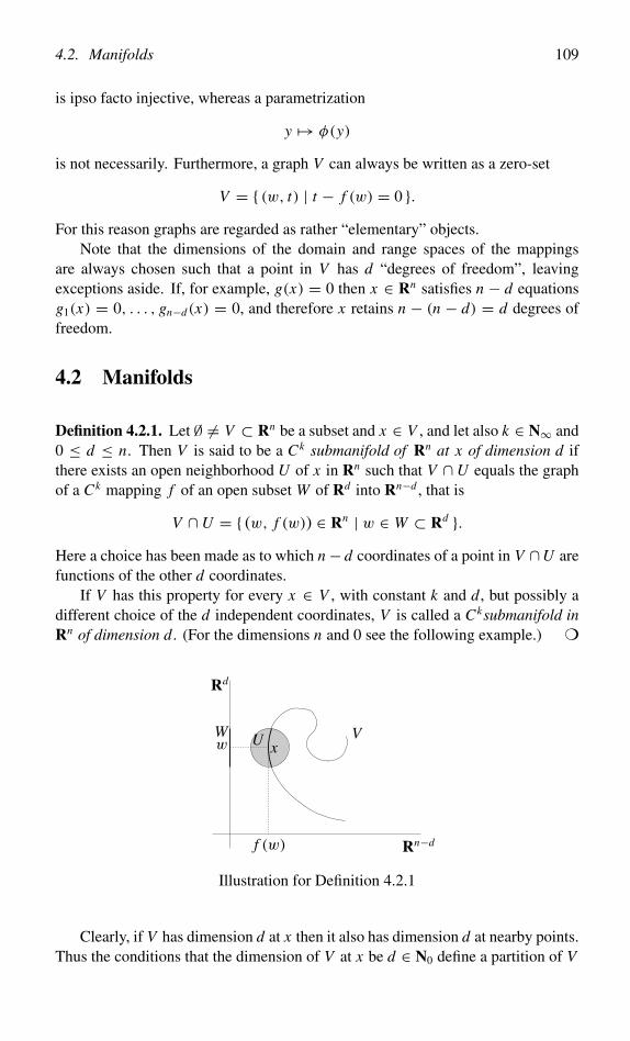
4.2. Manifolds 109
is ipso facto injective, whereas a parametrization
y �→ φ(y)
is not necessarily. Furthermore, a graph V can always be written as a zero-set
V = { (w, t) | t − f (w) = 0 }.For this reason graphs are regarded as rather “elementary” objects.
Note that the dimensions of the domain and range spaces of the mappingsare always chosen such that a point in V has d “degrees of freedom”, leavingexceptions aside. If, for example, g(x) = 0 then x ∈ Rn satisfies n − d equationsg1(x) = 0, . . . , gn−d(x) = 0, and therefore x retains n − (n − d) = d degrees offreedom.
4.2 Manifolds
Definition 4.2.1. Let ∅ = V ⊂ Rn be a subset and x ∈ V , and let also k ∈ N∞ and0 ≤ d ≤ n. Then V is said to be a Ck submanifold of Rn at x of dimension d ifthere exists an open neighborhood U of x in Rn such that V ∩U equals the graphof a Ck mapping f of an open subset W of Rd into Rn−d , that is
V ∩U = { (w, f (w)) ∈ Rn | w ∈ W ⊂ Rd }.Here a choice has been made as to which n− d coordinates of a point in V ∩U arefunctions of the other d coordinates.
If V has this property for every x ∈ V , with constant k and d, but possibly adifferent choice of the d independent coordinates, V is called a Cksubmanifold inRn of dimension d. (For the dimensions n and 0 see the following example.) ❍
f (w) Rn−d
wW VU x
Rd
Illustration for Definition 4.2.1
Clearly, if V has dimension d at x then it also has dimension d at nearby points.Thus the conditions that the dimension of V at x be d ∈ N0 define a partition of V
110 Chapter 4. Manifolds
into open subsets. Therefore, if V is connected, it has the same dimension at eachof its points.
If d = 1, we speak of a Ck curve; if d = 2, we speak of a Ck surface; and ifd = n − 1, we speak of a Ck hypersurface. According to these definitions curvesand (hyper)surfaces are sets; in subsequent parts of this book, however, the wordscurve or (hyper)surface may refer to mappings defining the sets.
Example 4.2.2. Every open subset V ⊂ Rn satisfies the definition of a C∞ subman-ifold in Rn of dimension n. Indeed, take W = V and define f : V → R0 = {0} byf (x) = 0, for all x ∈ V . Then x ∈ V can be identified with (x, f (x)) ∈ Rn×R0 �Rn . And likewise, every point in Rn is a C∞ submanifold in Rn of dimension 0.✰
Example 4.2.3. The unit sphere S2 ⊂ R3, with S2 = { x ∈ R3 | ‖x‖ = 1 }, is aC∞ submanifold in R3 of dimension 2. To see this, let x0 ∈ S2. The coordinatesof x0 cannot vanish all at the same time; so, for example, we may assume x0
2 = 0,say x0
2 < 0. One then has 1− (x01)
2 − (x03)
2 = (x02)
2 > 0, and therefore
x0 = (x01 , −
√1− (x0
1)2 − (x0
3)2, x0
3 ).
A similar description now is obtained for all points x ∈ S2 ∩ U , where U isthe neighborhood { x ∈ R3 | x2 < 0 } of x0 in R3. Indeed, let W be the openneighborhood { (x1, x3) ∈ R2 | x2
1 + x23 < 1 } of (x0
1 , x03) in R2, and further define
f : W → R by f (x1, x3) = −√
1− x21 − x2
3 .
Then f is a C∞ mapping because the polynomial under the root sign cannot attainthe value 0. In addition one has
S2 ∩U = { (x1, f (x1, x3), x3) | (x1, x3) ∈ W }.Subsequent permutation of coordinates shows S2 to satisfy the definition of a C∞submanifold of dimension 2 near x0. It will also be clear how to deal with the otherpossibilities for x0. ✰
As this example demonstrates, verifying that a set V satisfies the definition ofa submanifold can be laborious. We therefore subject the properties of manifoldsto further study; we will find sufficient conditions for V to be a manifold.
Remark 1. Let V be a Ck submanifold, for k ∈ N∞, in Rn of dimension d. Thendefine, in the notation of Definition 4.2.1, the mapping φ : W → Rn by
φ(w) = (w, f (w)).
4.2. Manifolds 111
Then φ is an injective Ck mapping, and therefore φ : W → φ(W ) is bijective. Theinverse mapping φ−1 : φ(W )→ W , with
(w, f (w)) �→ w
is continuous, because it is the projection mapping onto the first factor. In additionDφ(w), for w ∈ W , is injective because
Dφ(w) =
d
d
n−d
Id
D f (w)
.
Definition 4.2.4. Let D ⊂ Rd be a nonempty open subset, d ≤ n and k ∈ N∞, andφ ∈ Ck(D,Rn). Let y ∈ D, then φ is said to be a Ck immersion at y if
Dφ(y) ∈ Lin(Rd,Rn) is injective.
Further, φ is called a Ck immersion if φ is a Ck immersion at y, for all y ∈ D.A Ck immersion φ is said to be a Ck embedding if in addition φ is injective (note
that the induced mapping φ : D → φ(D) is bijective in that case), and if φ−1 :φ(D) → D is continuous. In particular, therefore, the mapping φ : D → φ(D)is bijective and continuous, and possesses a continuous inverse; in other words, itis a homeomorphism, see Definition 1.5.2. Accordingly, we can now say that a Ck
embedding φ : D → φ(D) is a Ck immersion which is also a homeomorphismonto its image.
Another way of saying this is that φ gives a Ck parametrization of φ(D) by D.Conversely, the mapping
κ := φ−1 : φ(D)→ D
is called a coordinatization or a chart for φ(D). ❍
Using Definition 4.2.4 we can reformulate Remark 1 above as follows. If V isa Ck submanifold for k ∈ N∞ in Rn of dimension d, there exists, for every x ∈ V ,a neighborhood U of x in Rn such that V ∩U possesses a Ck parametrization by ad-dimensional set. From the Immersion Theorem 4.3.1, which we shall presentlyprove, a converse result can be obtained. If φ : D → Rn is a Ck immersion at apoint y ∈ D, then φ(D) near x = φ(y) is a Ck submanifold in Rn of dimensiond = dim D. In other words, the image under a mapping φ that is an immersion aty is a submanifold near φ(y).
112 Chapter 4. Manifolds
Remark 2. Assume that V is a Ck submanifold of Rn at the point x0 ∈ V ofdimension d. If U and f are the neighborhood of x0 in Rn and the mapping fromDefinition 4.2.1, respectively, then every x ∈ U can be written as x = (w, t) withw ∈ W ⊂ Rd , t ∈ Rn−d ; we can further define the Ck mapping g by
g : U → Rn−d, g(x) = g(w, t) = t − f (w).
ThenV ∩U = { x ∈ U | g(x) = 0 }
andDg(x) ∈ Lin(Rn,Rn−d) is surjective, for all x ∈ U.
Indeed,
Dg(x) =(
Dwg(w, t) Dt g(w, t))=
d n−d
n−d
(− D f (w) In−d
).
Note that the surjectivity of Dg(x) implies that the column rank of Dg(x) equalsn − d. But then, in view of the Rank Lemma 4.2.7 below, the row rank also equalsn−d, which implies that the rows, Dg1(x), . . . , Dgn−d(x), are linearly independentvectors in Rn . Formulated in a different way: V ∩U can be described as the solutionset of n−d equations g1(x) = 0, . . . , gn−d(x) = 0 that are independent in the sensethat the system Dg1(x), . . . , Dgn−d(x) of vectors in Rn is linearly independent.
Definition 4.2.5. The number n − d of equations required for a local descriptionof V is called the codimension of V in Rn , notation
codimRn V = n − d. ❍
Definition 4.2.6. Let U ⊂ Rn be a nonempty open subset, d ∈ N0 and k ∈ N∞,and g ∈ Ck(U,Rn−d). Let x ∈ U , then g is said to be a Ck submersion at x if
Dg(x) ∈ Lin(Rn,Rn−d) is surjective.
Further, g is called a Ck submersion if g is a Ck submersion at x , for every x ∈ U .❍
Making use of Definition 4.2.6 we can reformulate the above Remark 2 asfollows. If V is a Ck manifold in Rn , there exists for every x ∈ V an openneighborhood U of x in Rn such that V ∩U is the zero-set of a Ck submersion, withvalues in a codimRn V -dimensional space. From the Submersion Theorem 4.5.2,which we shall prove later on, a converse result can be obtained. If g : U → Rn−d
4.2. Manifolds 113
is a Ck submersion at a point x ∈ U with g(x) = 0, then U ∩ g−1({0}) near x is aCk submanifold in Rn of dimension d. In other words, the inverse image under amapping g that is a submersion at x , of g(x), is a submanifold near x .
From linear algebra we recall the definition of the rank of A ∈ Lin(Rn,Rp)
as the dimension r of the image of A, which then satisfies r ≤ min(n, p). Weneed the result that A and its adjoint At ∈ Lin(Rp,Rn) have equal rank r . For thematrix of A with respect to the standard bases (e1, . . . , en) and (e′1, . . . , e′p) in Rn
and Rp, respectively, this means that the maximal number of linearly independentcolumns equals the maximal number of linearly independent rows. For the sake ofcompleteness we give an efficient proof of this result. Furthermore, in view of theprinciple that, locally near a point, a mapping behaves similar to its derivative atthe point in question, it suggests normal forms for mappings, as we will see in theImmersion and Submersion Theorems (and the Rank Theorem, see Exercise 4.35).
Lemma 4.2.7 (Rank Lemma). For A ∈ Lin(Rn,Rp) the following conditions areequivalent.
(i) A has rank r.
(ii) There exist � ∈ Aut(Rp) and � ∈ Aut(Rn) such that
� ◦ A ◦�(x) = (x1, . . . , xr , 0, . . . , 0) ∈ Rp (x ∈ Rn).
In particular, A and At have equal rank. Furthermore, if A is injective, then wemay arrange that � = I ; therefore in this case
� ◦ A(x) = (x1, . . . , xn, 0, . . . , 0) (x ∈ Rn).
On the other hand, suppose A is surjective. Then we can choose � = I ; therefore
A ◦�(x) = (x1, . . . , x p) (x ∈ Rn).
Finally, if A ∈ Aut(Rn), then we take either� or� equal to A−1, and the remainingoperator equal to I .
Proof. Only (i) ⇒ (ii) needs verification. In view of the equality dim(ker A) +r = n, we can find a basis (ar+1, . . . , an) of ker A ⊂ Rn and vectors a1, . . . , ar
complementing this basis to a basis of Rn . Define � ∈ Aut(Rn) setting �e j = a j ,for 1 ≤ j ≤ n. Then A�(e j ) = Aa j , for 1 ≤ j ≤ r , and A�(e j ) = 0, forr < j ≤ n. The vectors b j = Aa j , for 1 ≤ j ≤ r , form a basis of im A ⊂ Rp. Letus complement them by vectors br+1, . . . , bp to a basis of Rp. Define� ∈ Aut(Rp)
by �bi = e′i , for 1 ≤ i ≤ p. Then the operators � and � are the required ones,since
� ◦ A ◦�(e j ) ={
e′j , 1 ≤ j ≤ r;0, r < j ≤ n.
114 Chapter 4. Manifolds
The equality of ranks follows by means of the equality
� t ◦ At ◦�t(x1, . . . , x p) = (x1, . . . , xr , 0, . . . , 0) ∈ Rn.
If A is injective, then r = n and ker A = (0), and thus we choose � = I . If A issurjective, then r = p; we then select the complementary vectors a1, . . . , ap ∈ Rn
such that Aei = e′i , for 1 ≤ i ≤ p. Then � = I . ❏
4.3 Immersion Theorem
The following theorem says that, at least locally near a point y0, an immersion canbe given the same form as its derivative at y0 in the Rank Lemma 4.2.7.
Locally, an immersion φ : D0 → Rn with D0 an open subset of Rd , equals therestriction of a diffeomorphism of Rn to a linear subspace of dimension d. In fact,the Immersion Theorem asserts that there exist an open neighborhood D of y0 inD0 and a diffeomorphism � acting in the image space Rn , such that on D
φ = � ◦ ι,where ι : Rd → Rn denotes the standard embedding of Rd into Rn , defined by
ι (y1, . . . , yd) = (y1, . . . , yd, 0, . . . , 0).
Theorem 4.3.1 (Immersion Theorem). Let D0 ⊂ Rd be an open subset, let d < nand k ∈ N∞, and let φ : D0 → Rn be a Ck mapping. Let y0 ∈ D0, let φ(y0) = x0,and assume φ to be an immersion at y0, that is Dφ(y0) ∈ Lin(Rd,Rn) is injective.Then there exists an open neighborhood D of y0 in D0 such that the followingassertions hold.
(i) φ(D) is a Ck submanifold in Rn of dimension d.
(ii) There exist an open neighborhood U of x0 in Rn and a Ck diffeomorphism� : U → �(U ) ⊂ Rn such that for all y ∈ D
� ◦ φ(y) = (y, 0) ∈ Rd × Rn−d .
In particular, the restriction of φ to D is an injection.
Proof. (i). Because Dφ(y0) is injective, the rank of Dφ(y0) equals d. Conse-quently, among the rows of the matrix of Dφ(y0) there are d which are linearlyindependent. We assume that these are the top d rows (this may require priorpermutation of the coordinates of Rn). As a result we find Ck mappings
g : D0 → Rd and h : D0 → Rn−d, respectively,with
g = (φ1, . . . , φd), h = (φd+1, . . . , φn),
φ(D0) = { (g(y), h(y)) | y ∈ D0 },
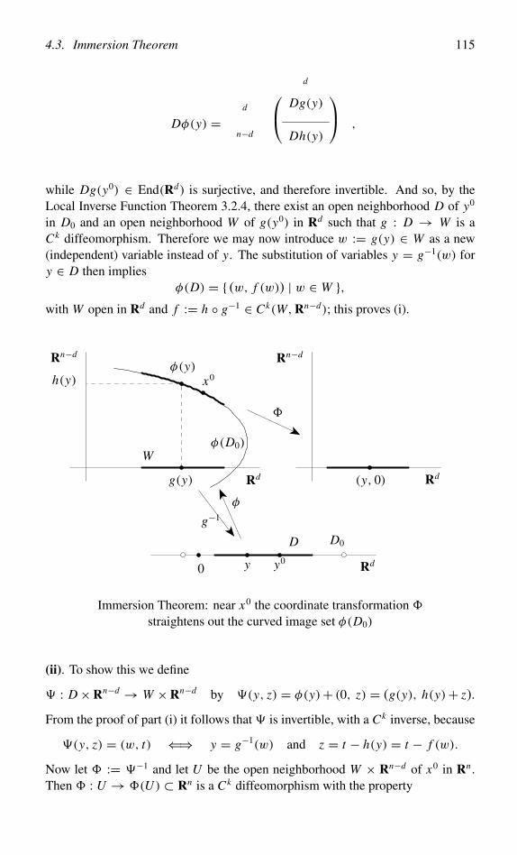
4.3. Immersion Theorem 115
Dφ(y) =
d
d
n−d
Dg(y)
Dh(y)
,
while Dg(y0) ∈ End(Rd) is surjective, and therefore invertible. And so, by theLocal Inverse Function Theorem 3.2.4, there exist an open neighborhood D of y0
in D0 and an open neighborhood W of g(y0) in Rd such that g : D → W is aCk diffeomorphism. Therefore we may now introduce w := g(y) ∈ W as a new(independent) variable instead of y. The substitution of variables y = g−1(w) fory ∈ D then implies
φ(D) = { (w, f (w)) | w ∈ W },with W open in Rd and f := h ◦ g−1 ∈ Ck(W,Rn−d); this proves (i).
0 y y0
D D0
Rd
(y, 0) Rd
Rn−d
h(y)
Rn−d
W
g(y)
φ(D0)
x0φ(y)
Rd
�
g−1
φ
Immersion Theorem: near x0 the coordinate transformation �straightens out the curved image set φ(D0)
(ii). To show this we define
� : D×Rn−d → W ×Rn−d by �(y, z) = φ(y)+ (0, z) = (g(y), h(y)+ z).
From the proof of part (i) it follows that � is invertible, with a Ck inverse, because
�(y, z) = (w, t) ⇐⇒ y = g−1(w) and z = t − h(y) = t − f (w).
Now let � := �−1 and let U be the open neighborhood W × Rn−d of x0 in Rn .Then � : U → �(U ) ⊂ Rn is a Ck diffeomorphism with the property
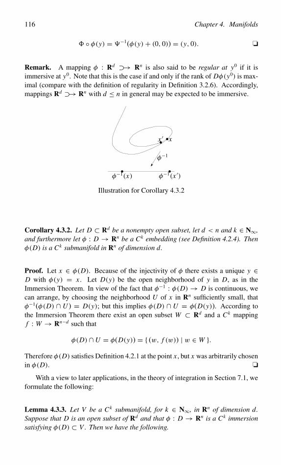
116 Chapter 4. Manifolds
� ◦ φ(y) = �−1(φ(y)+ (0, 0)) = (y, 0). ❏
Remark. A mapping φ : Rd ⊃→ Rn is also said to be regular at y0 if it isimmersive at y0. Note that this is the case if and only if the rank of Dφ(y0) is max-imal (compare with the definition of regularity in Definition 3.2.6). Accordingly,mappings Rd ⊃→ Rn with d ≤ n in general may be expected to be immersive.
x ′ x
φ−1(x) φ−1(x ′)
φ−1
Illustration for Corollary 4.3.2
Corollary 4.3.2. Let D ⊂ Rd be a nonempty open subset, let d < n and k ∈ N∞,and furthermore let φ : D → Rn be a Ck embedding (see Definition 4.2.4). Thenφ(D) is a Ck submanifold in Rn of dimension d.
Proof. Let x ∈ φ(D). Because of the injectivity of φ there exists a unique y ∈D with φ(y) = x . Let D(y) be the open neighborhood of y in D, as in theImmersion Theorem. In view of the fact that φ−1 : φ(D)→ D is continuous, wecan arrange, by choosing the neighborhood U of x in Rn sufficiently small, thatφ−1(φ(D) ∩ U ) = D(y); but this implies φ(D) ∩ U = φ(D(y)). According tothe Immersion Theorem there exist an open subset W ⊂ Rd and a Ck mappingf : W → Rn−d such that
φ(D) ∩U = φ(D(y)) = { (w, f (w)) | w ∈ W }.Therefore φ(D) satisfies Definition 4.2.1 at the point x , but x was arbitrarily chosenin φ(D). ❏
With a view to later applications, in the theory of integration in Section 7.1, weformulate the following:
Lemma 4.3.3. Let V be a Ck submanifold, for k ∈ N∞, in Rn of dimension d.Suppose that D is an open subset of Rd and that φ : D → Rn is a Ck immersionsatisfying φ(D) ⊂ V . Then we have the following.
4.3. Immersion Theorem 117
(i) φ(D) is an open subset of V (see Definition 1.2.16).
(ii) Furthermore, assume that φ is a Ck embedding. Let D be an open subset ofRd and let φ : D → Rn be a Ck mapping satisfying φ(D) ⊂ V . Then
Dφ,φ := φ−1(φ(D)) ⊂ D
is an open subset of Rd and φ−1 ◦ φ : Dφ,φ → D is a Ck mapping.
(iii) If, in addition, d = d and φ is a Ck embedding too, then we have a Ck
diffeomorphismφ−1 ◦ φ : Dφ,φ → Dφ,φ.
Proof. (i). Select x0 ∈ φ(D) arbitrarily and write x0 = φ(y0). Since x0 ∈ V , byDefinition 4.2.1 there exist an open neighborhood U0 of x0 in Rn , an open subsetW of Rd and a Ck mapping f : W → Rn−d such that V ∩ U0 = { (w, f (w)) ∈Rn | w ∈ W } (this may require prior permutation of the coordinates of Rn). ThenV0 := φ−1(U0) is an open neighborhood of y0 in D in view of the continuity of φ.As in the proof of the Immersion Theorem 4.3.1, we write φ = (g, h). Becauseφ(y) ∈ V ∩U0 for every y ∈ V0, we can find w ∈ W satisfying
(g(y), h(y)) = φ(y) = (w, f (w)),
thus w = g(y) and h(y) = f (w) = ( f ◦ g)(y).
Set w0 = g(y0). Because h = f ◦ g on the open neighborhood V0 of y0, the chainrule implies
Dh(y0) = D f (w0) Dg(y0).
This said, suppose v ∈ Rd satisfies Dg(y0)v = 0, then also Dh(y0)v = 0, whichimplies Dφ(y0)v = 0. In turn, this gives v = 0 because φ is an immersion at y0.Accordingly Dg(y0) ∈ End(Rd) is injective and so belongs to Aut(Rd). On thestrength of the Local Inverse Function Theorem 3.2.4 there exists an open neigh-borhood D0 of y0 in V0, such that the restriction of g to D0 is a Ck diffeomorphismonto an open neighborhood W0 of w0 in Rd . With these notations,
U (x0) := U0 ∩ (W0 × Rn−d)
is an open subset of Rn and φ(D0) = V ∩ U (x0). The union U of the open setsU (x0), for x0 varying in φ(D), is open in Rn while φ(D) = V ∩ U . This provesassertion (i).(ii). Assertion (i) now implies that
Dφ,φ = φ−1(φ(D)) = φ−1(V ∩U ) = φ−1(U ) ⊂ D
is an open subset of Rd , as φ : D → Rn is continuous and U ⊂ Rn is open. Lety0 ∈ Dφ,φ , write y0 = φ−1 ◦ φ(y0) and let D0 be the open neighborhood of y0 in D
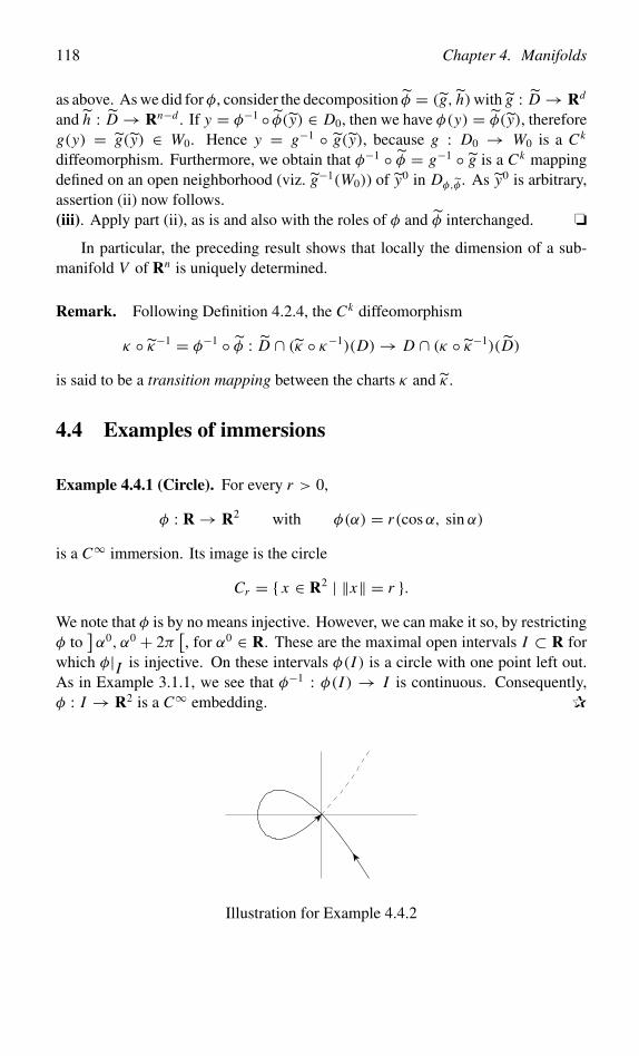
118 Chapter 4. Manifolds
as above. As we did forφ, consider the decomposition φ = (g, h)with g : D → Rd
and h : D → Rn−d . If y = φ−1 ◦ φ(y) ∈ D0, then we have φ(y) = φ(y), thereforeg(y) = g(y) ∈ W0. Hence y = g−1 ◦ g(y), because g : D0 → W0 is a Ck
diffeomorphism. Furthermore, we obtain that φ−1 ◦ φ = g−1 ◦ g is a Ck mappingdefined on an open neighborhood (viz. g−1(W0)) of y0 in Dφ,φ . As y0 is arbitrary,assertion (ii) now follows.(iii). Apply part (ii), as is and also with the roles of φ and φ interchanged. ❏
In particular, the preceding result shows that locally the dimension of a sub-manifold V of Rn is uniquely determined.
Remark. Following Definition 4.2.4, the Ck diffeomorphism
κ ◦ κ−1 = φ−1 ◦ φ : D ∩ (κ ◦ κ−1)(D)→ D ∩ (κ ◦ κ−1)(D)
is said to be a transition mapping between the charts κ and κ .
4.4 Examples of immersions
Example 4.4.1 (Circle). For every r > 0,
φ : R → R2 with φ(α) = r(cosα, sin α)
is a C∞ immersion. Its image is the circle
Cr = { x ∈ R2 | ‖x‖ = r }.We note that φ is by no means injective. However, we can make it so, by restrictingφ to
]α0, α0 + 2π
[, for α0 ∈ R. These are the maximal open intervals I ⊂ R for
which φ|I is injective. On these intervals φ(I ) is a circle with one point left out.As in Example 3.1.1, we see that φ−1 : φ(I ) → I is continuous. Consequently,φ : I → R2 is a C∞ embedding. ✰
Illustration for Example 4.4.2
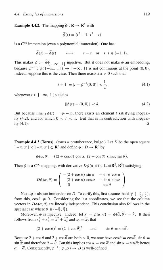
4.4. Examples of immersions 119
Example 4.4.2. The mapping φ : R → R2 with
φ(t) = (t2 − 1, t3 − t)
is a C∞ immersion (even a polynomial immersion). One has
φ(s) = φ(t) ⇐⇒ s = t or s, t ∈ {−1, 1}.This makes φ := φ|]−∞, 1 [ injective. But it does not make φ an embedding,
because φ−1 : φ( ]−∞, 1 [ ) → ]−∞, 1 [ is not continuous at the point (0, 0).Indeed, suppose this is the case. Then there exists a δ > 0 such that
|t + 1| = |t − φ−1(0, 0)| < 1
2, (4.1)
whenever t ∈ ]−∞, 1 [ satisfies
‖φ(t)− (0, 0)‖ < δ. (4.2)
But because limt↑1 φ(t) = φ(−1), there exists an element t satisfying inequal-ity (4.2), and for which 0 < t < 1. But that is in contradiction with inequal-ity (4.1). ✰
Example 4.4.3 (Torus). (torus = protuberance, bulge.) Let D be the open square]−π, π [× ]−π, π [ ⊂ R2 and define φ : D → R3 by
φ(α, θ) = ((2+ cos θ) cosα, (2+ cos θ) sin α, sin θ).
Then φ is a C∞ mapping, with derivative Dφ(α, θ) ∈ Lin(R2,R3) satisfying
Dφ(α, θ) = −(2+ cos θ) sin α − sin θ cosα
(2+ cos θ) cosα − sin θ sin α0 cos θ
.
Next, φ is also an immersion on D. To verify this, first assume that θ /∈ {−π2 ,
π2 };
from this, cos θ = 0. Considering the last coordinates, we see that the columnvectors in Dφ(α, θ) are linearly independent. This conclusion also follows in thespecial case where θ ∈ {−π
2 ,π2 }.
Moreover, φ is injective. Indeed, let x = φ(α, θ) = φ(α, θ) = x . It thenfollows from x2
1 + x22 = x2
1 + x22 and x3 = x3 that
(2+ cos θ)2 = (2+ cos θ )2 and sin θ = sin θ .
Because 2+ cos θ and 2+ cos θ are both > 0, we now have cos θ = cos θ , sin θ =sin θ ; and therefore θ = θ . But this implies cosα = cos α and sin α = sin α; henceα = α. Consequently, φ−1 : φ(D)→ D is well-defined.
120 Chapter 4. Manifolds
Finally, we prove the continuity of φ−1 : φ(D)→ D. If φ(α, θ) = x , then
(cosα, sin α) = (x21 + x2
2)−1/2 (x1, x2) =: h(x),
(cos θ, sin θ) = ((x21 + x2
2)1/2 − 2, x3) =: k(x).
Here h, k : φ(D) → R2 are continuous mappings. The inverse of the mappingβ �→ (cosβ, sin β) (β ∈ ]−π, π [) is given by g(u) := 2 arctan ( u2
1+u1); and this
mapping g also is continuous. Hence
(α, θ) = (g ◦ h(x), g ◦ k(x)),
which shows φ−1 : x �→ (α, θ) to be a continuous mapping φ(D)→ D.It follows that φ : D → R3 is an embedding, and according to Corollary 4.3.2
the image φ(D) is a C∞ submanifold in R3 of dimension 2. Verify that φ(D) lookslike the surface of a torus (donut) minus two intersecting circles. ✰
Illustration for Example 4.4.3: Transparent torus
4.5 Submersion Theorem
The following theorem says that, at least locally near a point x0, a submersion canbe given the same form as its derivative at x0 in the Rank Lemma 4.2.7.
Locally, a submersion g : U0 → Rn−d with U0 an open subset in Rn , equals adiffeomorphism of Rn followed by projection onto a linear subspace of dimensionn−d. In fact, the Submersion Theorem asserts that there exist an open neighborhoodU of x0 in U0 and a diffeomorphism � acting in the domain space Rn , such thaton U ,
g = π ◦�,
4.5. Submersion Theorem 121
where π : Rn → Rn−d denotes the standard projection onto the last n − d coordi-nates, defined by
π(x1, . . . , xn) = (xd+1, . . . , xn).
Example 4.5.1. Let g1 : R3 → R with g1(x) = ‖x‖2, and g2 : R3 → R withg2(x) = x3 be given functions. Assume, for (c1, c2) in a neighborhood of (1, 0),that a point x ∈ R3 satisfies g1(x) = c1 and g2(x) = c2; that point x then lies onthe intersection of a sphere and a plane, in other words, on a circle. Locally, such apoint x is then uniquely determined by prescribing the coordinate x1. Instead of theCartesian coordinates (x1, x2, x3), one may therefore also use the coordinates (y, c)on R3 to characterize x , where in the present case y = y1 = x1 and c = (c1, c2).Accordingly, this leads to a substitution of variables x = �(y, c) in R3. Note thatin these (y, c)-coordinates a circle is locally described as the linear submanifold ofR3 given by c equals a constant vector.
The notion that, locally at least, a point x ∈ Rn may uniquely be determined bythe values (c1, . . . , cn−d) taken by n− d functions g1, …, gn−d at x , plus a suitablechoice of d Cartesian coordinates (y1, . . . , yd) of x , is fundamental to the followingSubmersion Theorem 4.5.2. ✰
We recall the following definition from Theorem 1.3.7. Let U ⊂ Rn and letg : U → Rp. For all c ∈ Rp we define level set N (c) by
N (c) = N (g, c) = { x ∈ U | g(x) = c }.
Theorem 4.5.2 (Submersion Theorem). Let U0 ⊂ Rn be an open subset, let1 ≤ d < n and k ∈ N∞, and let g : U0 → Rn−d be a Ck mapping. Let x0 ∈ U0, letg(x0) = c0, and assume g to be a submersion in x0, that is Dg(x0) ∈ Lin(Rn,Rn−d)
is surjective. Then there exist an open neighborhood U of x0 in U0 and an openneighborhood C of c0 in Rn−d such that the following hold.
(i) The restriction of g to U is an open surjection.
(ii) The set N (c) ∩U is a Ck submanifold in Rn of dimension d, for all c ∈ C.
(iii) There exists a Ck diffeomorphism� : U → Rn such that�maps the manifoldN (c) ∩U in Rn into the linear submanifold of Rn given by
{ (x1, . . . , xn) ∈ Rn | (xd+1, . . . , xn) = c }.
(iv) There exists a Ck diffeomorphism � : �(U )→ U such that
g ◦�(y) = (yd+1, . . . , yn).
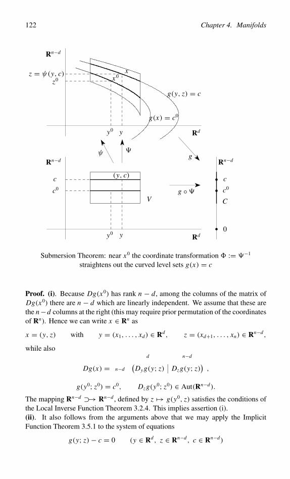
122 Chapter 4. Manifolds
y0 y Rd
V
(y, c)
c0
c
Rn−d
0
C
c0
c
Rn−d
g ◦�
g
g(x) = c0
�ψ
y0 y Rd
g(y, z) = c
xx0
z0z = ψ(y, c)
Rn−d
Submersion Theorem: near x0 the coordinate transformation � := �−1
straightens out the curved level sets g(x) = c
Proof. (i). Because Dg(x0) has rank n − d, among the columns of the matrix ofDg(x0) there are n − d which are linearly independent. We assume that these arethe n−d columns at the right (this may require prior permutation of the coordinatesof Rn). Hence we can write x ∈ Rn as
x = (y, z) with y = (x1, . . . , xd) ∈ Rd, z = (xd+1, . . . , xn) ∈ Rn−d,
while also
Dg(x) =d n−d
n−d(Dyg(y; z) Dzg(y; z)
),
g(y0; z0) = c0, Dzg(y0; z0) ∈ Aut(Rn−d).
The mapping Rn−d ⊃→ Rn−d , defined by z �→ g(y0, z) satisfies the conditions ofthe Local Inverse Function Theorem 3.2.4. This implies assertion (i).(ii). It also follows from the arguments above that we may apply the ImplicitFunction Theorem 3.5.1 to the system of equations
g(y; z)− c = 0 (y ∈ Rd, z ∈ Rn−d, c ∈ Rn−d)
4.5. Submersion Theorem 123
in the unknown z with y and c as parameters. Accordingly, there exist η, γ andζ > 0 such that for every
(y, c) ∈ V := { (y, c) ∈ Rd × Rn−d | ‖y − y0‖ < η, ‖c − c0‖ < γ }
there is a unique z = ψ(y, c) ∈ Rn−d satisfying
(y, z) ∈ U0, ‖z − z0‖ < ζ, g(y; z) = c.
Moreover, ψ : V → Rn−d , defined by (y, c) �→ ψ(y, c), is a Ck mapping. If wenow define C := { c ∈ Rn−d | ‖c − c0‖ < γ }, we have, for c ∈ C
N (c) ∩ { (y, z) ∈ Rn | ‖y − y0‖ < η, ‖z − z0‖ < ζ }= { (y, ψ(y, c)) | ‖y − y0‖ < η }.
Locally, therefore, and with c constant, N (c) is the graph of the Ck function y �→ψ(y, c) with an open domain in Rd ; but this proves (ii).(iii). Define
� : U0 → Rn by �(y, z) = (y, g(y; z)).
From the proof of part (ii) we then have �(y, z) = (y, c) ∈ V if and only if(y, z) = (y, ψ(y, c)). It follows that, locally in a neighborhood of x0, the mapping� is invertible with a Ck inverse. In other words, there exists an open neighborhoodU of x0 in U0 such that � : U → V is a Ck diffeomorphism of open sets in Rn .For (y, z) ∈ N (c) ∩ U we have g(y; z) = c; and so �(y, z) = (y, c). Thereforewe have now proved (iii).(iv). Finally, let � := �−1 : V → U . Because �(y, z) = (y, c) if and only ifg(y; z) = c, one has for (y, c) ∈ V
g ◦�(y, c) = g(y, z) = c.
Finally we note that in Exercise 7.36 we make use of the fact that one mayassume, if d = n − 1 (and for smaller values of η and γ > 0 if necessary), that Vis the open set in Rn with
V := { (y, c) ∈ Rn−1 × R | ‖y − y0‖ < η, |c − c0| < γ },
and that U is the open neighborhood of x0 in Rn defined by
U := { (y, z) ∈ Rn−1 × R | ‖y − y0‖ < η, |g(y; z)− c0| < γ }.
To prove this, show by means of a first-order Taylor expansion that the estimate‖z − z0‖ < ζ follows from an estimate of the type |g(y; z) − c0| < γ , becauseDzg(y0; z0) = 0. ❏
124 Chapter 4. Manifolds
Remark. A mapping g : Rn ⊃→ Rn−d is also said to be regular at x0 if it issubmersive at x0. Note that this is the case if and only if rank Dg(x0) is maximal(compare with the definitions of regularity in Sections 3.2 and 4.3). Accordingly,mappings Rn ⊃→ Rn−d with d ≥ 0 in general may be expected to be submersive.
If g(x0) = c0, then N (c0) is also said to be the fiber of the mapping g belongingto the value c0. For regular x0 this therefore looks like a manifold. The fibers N (c)together form a fiber bundle: under the diffeomorphism � from the SubmersionTheorem they are locally transferred into the linear submanifolds of Rn given bythe last n − d coordinates being constant.
4.6 Examples of submersions
Example 4.6.1 (Unit sphere Sn−1). (See Example 4.2.3). The unit sphere
Sn−1 = { x ∈ Rn | ‖x‖ = 1 }is a C∞ submanifold in Rn of dimension n − 1. Indeed, defining the C∞ mappingg : Rn → R by
g(x) = ‖x‖2,
one has Sn−1 = N (1). Let x0 ∈ Sn−1, then
Dg(x0) ∈ Lin(Rn,R) given by Dg(x0) = 2x0
is surjective, x0 being different from 0. But then, according to the SubmersionTheorem there exists a neighborhood U of x0 in Rn such that Sn−1 ∩ U is a C∞submanifold in Rn of dimension n − 1.
More generally, the Submersion Theorem asserts that, locally near x0, the fiberN (g(x0)) can be described by writing a suitably chosen xi as a C∞ function of thex j with j = i . ✰
Example 4.6.2 (Orthogonal matrices). The set O(n,R), the orthogonal group,consisting of the orthogonal matrices in Mat(n,R) � Rn2
, with
O(n,R) = { A ∈ Mat(n,R) | At A = I }is a C∞ manifold of dimension 1
2 n(n−1) in Mat(n,R). Let Mat+(n,R) be the linearsubspace in Mat(n,R) consisting of the symmetric matrices. Note that A = (ai j ) ∈Mat+(n,R) if and only if ai j = a ji . This means that A is completely determined bythe ai j with i ≥ j , of which there are 1+ 2+ · · · + n = 1
2 n(n + 1). Consequently,Mat+(n,R) is a linear subspace of Mat(n,R) of dimension 1
2 n(n + 1). We have
O(n,R) = g−1({I }),
4.6. Examples of submersions 125
where g : Mat(n,R)→ Mat+(n,R) is the mapping with
g(A) = At A.
Note that indeed (At A)t = At Att = At A. We shall now prove that g is a submersionat every A ∈ O(n,R). Since Mat(n,R) and Mat+(n,R) are linear spaces, we maywrite, for every A ∈ O(n,R)
Dg(A) : Mat(n,R)→ Mat+(n,R).
Observe that g can be written as the composition A �→ (A, A) �→ At A = g(A, A),where g : (A1, A2) �→ At
1 A2 is bilinear, that is g ∈ Lin2 ( Mat(n,R),Mat(n,R)).Using Proposition 2.7.6 we now obtain, with H ∈ Mat(n,R),
Dg(A) : H �→ (H, H) �→ g(H, A)+ g(A, H) = H t A + At H.
Therefore, the surjectivity of Dg(A) follows if, for every C ∈ Mat+(n,R), we canfind a solution H ∈ Mat(n,R) of H t A + At H = C . Now C = 1
2 Ct + 12 C . So we
try to solve H from
H t A = 1
2Ct and At H = 1
2C; hence H = 1
2(A−1)tC = 1
2AC.
We now see that the conditions of the Submersion Theorem are satisfied; therefore,near A ∈ O(n,R) the subset O(n,R) = g−1({I }) of Mat(n,R) is a C∞ manifoldof dimension equal to
dim Mat(n,R)− dim Mat+(n,R) = n2 − 1
2n(n + 1) = 1
2n(n − 1).
Because this is true for every A ∈ O(n,R) the assertion follows. ✰
Example 4.6.3 (Torus). We come back to Example 4.4.3. There an open subsetV of a toroidal surface T was given as a parametrized set, that is, as the imageV = φ(D) under φ : D = ]−π, π [× ]−π, π [ → R3 with
φ(α, θ) = x = ((2+ cos θ) cosα, (2+ cos θ) sin α, sin θ). (4.3)
We now try to write the set V , or, if we have to, a somewhat larger set, as the zero-setof a function g : R3 → R to be determined. To achieve this, we eliminate α and θfrom Formula (4.3), that is to say, we try to find a relation between the coordinatesx1, x2 and x3 of x which follows from the fact that x ∈ V . We have, for x ∈ V ,
x21 = (2+ cos θ)2 cos2 α, x2
2 = (2+ cos θ)2 sin2 α, x23 = sin2 θ.
This gives
‖x‖2 = (2+ cos θ)2 + sin2 θ = 4+ 4 cos θ + cos2 θ + sin2 θ = 5+ 4 cos θ.
126 Chapter 4. Manifolds
Therefore (‖x‖2 − 5)2 = 16 cos2 θ and 16x23 = 16 sin2 θ . And so
(‖x‖2 − 5)2 + 16x23 = 16. (4.4)
There is a problem, however, in that we have only proved that every x ∈ V satisfiesequation (4.4). Conversely, it can be shown that the toroidal surface T appears asthe zero-set N of the function g : R3 → R, defined by
g(x) = (‖x‖2 − 5)2 + 16(x23 − 1).
(The proof, which is not very difficult, is not given here.) Next, we examine whetherg is submersive at the points x ∈ N . For this to be so, Dg(x) ∈ Lin(R3,R) mustbe of rank 1, which is in fact the case except when
Dg(x) = 4(x1(‖x‖2 − 5), x2(‖x‖2 − 5), x3(‖x‖2 + 3)) = 0.
This immediately implies x3 = 0. Also, it follows from the first two coefficientsthat ‖x‖2 − 5 = 0, because x = 0 does not satisfy equation (4.4). But theseconditions on x ∈ N violate equation (4.4); consequently, g is submersive in all ofN . By the Submersion Theorem it now follows that N is a C∞ submanifold in R3
of dimension 2. ✰
4.7 Equivalent definitions of manifold
The preceding yields the useful result that the local descriptions of a manifold as agraph, as a parametrized set, as a zero-set, and as a set which locally looks like Rd
and which is “flat” in Rn , are all entirely equivalent.
Theorem 4.7.1. Let V be a subset of Rn and let x ∈ V , and suppose 0 ≤ d ≤ nand k ∈ N∞. Then the following four assertions are equivalent.
(i) There exist an open neighborhood U in Rn of x, an open subset W of Rd anda Ck mapping f : W → Rn−d such that
V ∩U = graph( f ) = { (w, f (w)) ∈ Rn | w ∈ W }.
(ii) There exist an open neighborhood U in Rn of x, an open subset D of Rd anda Ck embedding φ : D → Rn such that
V ∩U = im(φ) = {φ(y) ∈ Rn | y ∈ D }.
4.7. Equivalent definitions of manifold 127
(iii) There exist an open neighborhood U in Rn of x and a Ck submersion g :U → Rn−d such that
V ∩U = N (g, 0) = { u ∈ U | g(u) = 0 }.
(iv) There exist an open neighborhood U in Rn of x, a Ck diffeomorphism � :U → Rn and an open subset Y of Rd such that
�(V ∩U ) = Y × {0Rn−d }.
Proof. (i)⇒ (ii) is Remark 1 in Section 4.2. (ii)⇒ (i) is Corollary 4.3.2. (i)⇒ (iii)is Remark 2 in Section 4.2. (iii) ⇒ (i) and (iii) ⇒ (iv) follow by the SubmersionTheorem 4.5.2, and (iv)⇒ (ii) is trivial. ❏
Remark. Which particular description of a manifold V to choose will depend onthe circumstances; the way in which V is initially given is obviously important. Butthere is a rule of thumb:
• when the “internal” structure of V is important, as in the integration over Vin Chapters 7 or 8, a description as an image under an embedding or as agraph is useful;
• when one wishes to study the “external” structure of V , for example, what isthe location of V with respect to the ambient space Rn , the description as azero-set often is to be preferred.
Corollary 4.7.2. Suppose V is a Ck submanifold in Rn of dimension d and � :Rn ⊃→ Rn is a Ck diffeomorphism which is defined on an open neighborhood ofV , then �(V ) is a Ck submanifold in Rn of dimension d too.
Proof. We use the local description V ∩U = im(φ) according to Theorem 4.7.1.(ii).Then
�(V ) ∩�(U ) = �(V ∩U ) = im(� ◦ φ),where � ◦ φ : D → Rn is a Ck embedding, since φ is so. ❏
In fact, we can introduce the notion of a Ck mapping of manifolds withoutrecourse to ambient spaces.
128 Chapter 4. Manifolds
Definition 4.7.3. Suppose V is a submanifold in Rn of dimension d, and V ′ asubmanifold in Rn′ of dimension d ′, and let k ∈ N∞. A mapping of manifolds� : V → V ′ is said to be a Ck mapping if for every x ∈ V there exist neighborhoodsU of x in Rn , and U ′ of �(x) in Rn′ , open sets D ⊂ Rd , and D′ ⊂ Rd ′ , and Ck
embeddings φ : D → V ∩U , and φ′ : D′ → V ′ ∩U ′, respectively, such that
φ′−1 ◦� ◦ φ : D ⊃→ Rd ′
is a Ck mapping. It is a consequence of Lemma 4.3.3.(iii) that the particular choicesof the embeddings φ and φ′ in this definition are irrelevant. ❍
This definition hints at a theory of manifolds that does not require a manifold apriori to be a subset of some ambient space Rn . In such a theory, all properties ofmanifolds are formulated in terms of the embeddings φ or the charts κ = φ−1.
Remark. To say that a subset V of Rn is a smooth d-dimensional submanifold isto make a statement about the local behavior of V . A global, algebraic, variant ofthe characterization as a zero-set is the following definition: V ⊂ Rn is said to bean algebraic submanifold of Rn if there are polynomials g1, . . . , gn−d in n variablesfor which
V = { x ∈ Rn | gi (x) = 0, 1 ≤ i ≤ n − d }.Here, on account of the algebraic character of the definition, R may be replacedby an arbitrary number system (field) k. Because kn is the standard model ofthe n-dimensional affine space (over the field k), the terminology affine algebraicmanifold V is also used; further, if k = R, this manifold is said to be real. Whendoing so, one can also formulate the dimension of V , as well as its being smooth(where applicable), in purely algebraic terms; this will not be pursued here (but seeExercise 5.76). Still, it will be clear that if k = R and if Dg1(x), . . . , Dgn−d(x), forevery x ∈ V , are linearly independent, the real affine algebraic manifold V is alsosmooth, and of dimension d. Without the assumption about the gradients, V canhave interesting singularities, one example being the quadratic cone x2
1+ x22− x2
3 =0 in R3. Note that V is always a closed subset of Rn because polynomials arecontinuous functions.
4.8 Morse’s Lemma
Let U ⊂ Rn be open and f ∈ Ck(U ) with k ≥ 1. In Theorem 2.6.3.(iv) wehave seen that x0 ∈ U is a critical point of f if f attains a local extremum at x0.Generally, x0 is said to be a singular (= nonregular, because nonsubmersive, (seethe Remark at the end of Section 4.5) or critical point of f if grad f (x0) = 0. Fromthe Submersion Theorem 4.5.2 we know that near regular points the level surfaces
N (c) = { x ∈ U | f (x) = c }
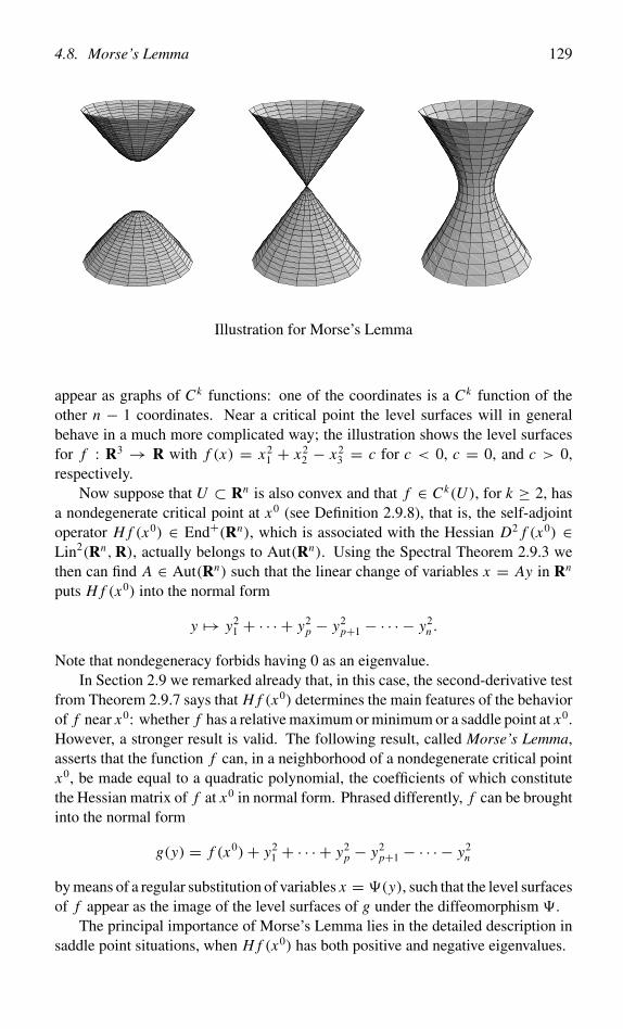
4.8. Morse’s Lemma 129
Illustration for Morse’s Lemma
appear as graphs of Ck functions: one of the coordinates is a Ck function of theother n − 1 coordinates. Near a critical point the level surfaces will in generalbehave in a much more complicated way; the illustration shows the level surfacesfor f : R3 → R with f (x) = x2
1 + x22 − x2
3 = c for c < 0, c = 0, and c > 0,respectively.
Now suppose that U ⊂ Rn is also convex and that f ∈ Ck(U ), for k ≥ 2, hasa nondegenerate critical point at x0 (see Definition 2.9.8), that is, the self-adjointoperator H f (x0) ∈ End+(Rn), which is associated with the Hessian D2 f (x0) ∈Lin2(Rn,R), actually belongs to Aut(Rn). Using the Spectral Theorem 2.9.3 wethen can find A ∈ Aut(Rn) such that the linear change of variables x = Ay in Rn
puts H f (x0) into the normal form
y �→ y21 + · · · + y2
p − y2p+1 − · · · − y2
n .
Note that nondegeneracy forbids having 0 as an eigenvalue.In Section 2.9 we remarked already that, in this case, the second-derivative test
from Theorem 2.9.7 says that H f (x0) determines the main features of the behaviorof f near x0: whether f has a relative maximum or minimum or a saddle point at x0.However, a stronger result is valid. The following result, called Morse’s Lemma,asserts that the function f can, in a neighborhood of a nondegenerate critical pointx0, be made equal to a quadratic polynomial, the coefficients of which constitutethe Hessian matrix of f at x0 in normal form. Phrased differently, f can be broughtinto the normal form
g(y) = f (x0)+ y21 + · · · + y2
p − y2p+1 − · · · − y2
n
by means of a regular substitution of variables x = �(y), such that the level surfacesof f appear as the image of the level surfaces of g under the diffeomorphism �.
The principal importance of Morse’s Lemma lies in the detailed description insaddle point situations, when H f (x0) has both positive and negative eigenvalues.
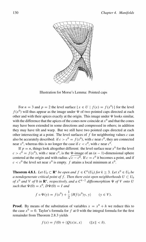
130 Chapter 4. Manifolds
Illustration for Morse’s Lemma: Pointed caps
For n = 3 and p = 2 the level surface { x ∈ U | f (x) = f (x0) } for the levelf (x0) will thus appear as the image under � of two pointed caps directed at eachother and with their apices exactly at the origin. This image under � looks similar,with the difference that the apices of the cones now coincide at x0 and that the conesmay have been extended in some directions and compressed in others; in additionthey may have tilt and warp. But we still have two pointed caps directed at eachother intersecting at a point. The level surfaces of f for neighboring values c canalso be accurately described: if c > c0 = f (x0), with c near c0, they are connectednear x0, whereas this is no longer the case if c < c0, with c near c0.
If p = n, things look altogether different: the level surface near x0 for the levelc > c0 = f (x0), with c near c0, is the �-image of an (n − 1)-dimensional spherecentered at the origin and with radius
√c − c0. If c = c0 it becomes a point, and if
c < c0 the level set near x0 is empty. f attains a local minimum at x0.
Theorem 4.8.1. Let U0 ⊂ Rn be open and f ∈ Ck(U0) for k ≥ 3. Let x0 ∈ U0 bea nondegenerate critical point of f . Then there exist open neighborhoods U ⊂ U0
of x0 and V of 0 in Rn, respectively, and a Ck−2 diffeomorphism � of V onto Usuch that �(0) = x0, D�(0) = I and
f ◦�(y) = f (x0)+ 1
2〈H f (x0)y, y〉 (y ∈ V ).
Proof. By means of the substitution of variables x = x0 + h we reduce this tothe case x0 = 0. Taylor’s formula for f at 0 with the integral formula for the firstremainder from Theorem 2.8.3 yields
f (x) = f (0)+ 〈Q(x)x, x〉 (‖x‖ < δ).
4.8. Morse’s Lemma 131
Here δ > 0 has been chosen sufficiently small; and
Q(x) =∫ 1
0(1− t) H f (t x) dt ∈ End(Rn)
has Ck−2 dependence on x , while Q(0) = 12 H f (0). Next it follows from The-
orem 2.7.9 that H f (0), and hence also Q(0) ∈ End+(Rn), in other words, theseoperators are self-adjoint. We now wish to find out whether we may write
〈Q(x)x, x〉 = 〈Q(0)y, y〉with y = A(x)x , where A(x) ∈ End(Rn) is suitably chosen. Because
〈Q(0) ◦ A(x)x, A(x)x〉 = 〈A(x)t ◦ Q(0) ◦ A(x)x, x〉,we see that this can be arranged by ensuring that A = A(x) satisfies the equation
F(A, x) := At ◦ Q(0) ◦ A − Q(x) = 0.
Now F(I, 0) = 0, and it proves convenient to try A = I + 12 Q(0)−1 B with
B ∈ End+(Rn), near 0. In other words, we switch to the equation
0 = G(B, x) := (I + 12 Q(0)−1 B)t ◦ Q(0) ◦ (I + 1
2 Q(0)−1 B)− Q(x)
= B + 14 B ◦ Q(0)−1 ◦ B + Q(0)− Q(x).
Now G(0, 0) = 0, and DB(0, 0) equals the identity mapping of the linear spaceEnd+(Rn) into itself. Application of the Implicit Function Theorem 3.5.1 givesan open neighborhood U1 of 0 in Rn and a Ck−2 mapping B from U1 into thelinear space End+(Rn) with B(0) = 0 and G(B(x), x) = 0, for all x ∈ U1.Writing �(x) = A(x)x = (I + 1
2 Q(0)−1 B(x))x , we then have � ∈ Ck−2(U1,Rn),�(0) = 0 and D�(0) = I . Furthermore,
〈Q(x)x, x〉 = 〈Q(0) ◦�(x), �(x)〉 (x ∈ U1).
By the Local Inverse Function Theorem 3.2.4 there is an open U ⊂ U1 around 0such that �|U is a Ck−2 diffeomorphism onto an open neighborhood V of 0 in Rn .Now � = (�|U )−1 meets all requirements. ❏
Lemma 4.8.2 (Morse). Let the notation be as in Theorem 4.8.1. We make thefurther assumption that among the eigenvalues of H f (x0) there are p that arepositive and n − p that are negative. Then there exist open neighborhoods U of x0
and W of 0, respectively, in Rn, and a Ck−2 diffeomorphism � from W onto U suchthat �(0) = x0 and
f ◦�(w) = f (x0)+ w21 + · · · + w2
p − w2p+1 − · · · − w2
n (w ∈ W ).
132 Chapter 4. Manifolds
Proof. Letλ1, . . . , λn be the (real) eigenvalues of H f (x0) ∈ End+(Rn), each eigen-value being repeated a number of times equal to its multiplicity, with λ1, . . . , λp
positive and λp+1, . . . , λn negative. From Formula (2.29) it is known that there isan orthogonal operator O ∈ O(Rn) such that
1
2〈H f (x0) ◦ Oz, Oz〉 = 1
2
∑1≤ j≤n
λ j z2j .
Under the substitution z j = (2/|λ j |) 12w j this takes the form
w21 + · · · + w2
p − w2p+1 − · · · − w2
n.
If P ∈ End(Rn) has a diagonal matrix with Pj j = (2/|λ j |) 12 , Morse’s Lemma
immediately follows from the preceding theorem by writing � = � ◦ O ◦ P . ❏
Note that D�(0) = O P; this information could have been added to Morse’sLemma. Here P is responsible for the “extension” or the “compression”, respec-tively, in the various directions, and O for the “tilt”. The terms of higher order inthe Taylor expansion of � at 0 are responsible for the “warp” of the level surfacesdiscussed in the introduction.
Remark. At this stage, Theorem 2.9.7 in the case of a nondegenerate critical pointis a consequence of Morse’s Lemma.
Chapter 5
Tangent Spaces
Differentiable mappings can be approximated by affine mappings; similarly, man-ifolds can locally be approximated by affine spaces, which are called (geometric)tangent spaces. These spaces provide enhanced insight into the structure of themanifold. In Volume II, in Chapter 7 the concept of tangent space plays an essentialrole in the integration on a manifold; the same applies to the study of the boundaryof an open set, an important subject in the extension of the Fundamental Theoremof Calculus to higher-dimensional spaces. In this chapter we consider various otherapplications of tangent spaces as well: cusps, normal vectors, extrema of the re-striction of a function to a submanifold, and the curvature of curves and surfaces.We close this chapter with introductory remarks on one-parameter groups of diffeo-morphisms, and on linear Lie groups and their Lie algebras, which are importanttools in describing continuous symmetry.
5.1 Definition of tangent space
Let k ∈ N∞, let V be a Ck submanifold in Rn of dimension d and let x ∈ V . Wewant to define the (geometric) tangent space of V at the point x ; this is, locally atx , the “best” approximation of V by a d-dimensional affine manifold (= translatedlinear subspace). In Section 2.2 we encountered already the description of thetangent space of graph( f ) at the point (w, f (w)) as the graph of the affine mappingh �→ f (w)+D f (w)h. In the following definition of the tangent space of a manifoldat a point, however, we wish to avoid the assumption of a graph as the only localdescription of the manifold. This is why we shall base our definition of tangentspace on the concept of tangent vector of a curve in Rn , which we introduce in thefollowing way.
Let I ⊂ R be an open interval and let γ : I → Rn be a differentiable mapping.
133
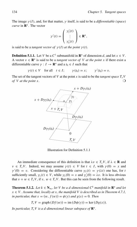
134 Chapter 5. Tangent spaces
The image γ (I ), and, for that matter, γ itself, is said to be a differentiable (space)curve in Rn . The vector
γ ′(t) = γ ′1(t)
...
γ ′n(t)
∈ Rn,
is said to be a tangent vector of γ (I ) at the point γ (t).
Definition 5.1.1. Let V be a C1 submanifold in Rn of dimension d, and let x ∈ V .A vector v ∈ Rn is said to be a tangent vector of V at the point x if there exist adifferentiable curve γ : I → Rn and a t0 ∈ I such that
γ (t) ∈ V for all t ∈ I ; γ (t0) = x; γ ′(t0) = v.
The set of the tangent vectors of V at the point x is said to be the tangent space Tx Vof V at the point x . ❍
Tx V
0
Dγ1(t0)
Dγ2(t0)
x + Tx V
γ2
γ1
x + Dγ1(t0)
x + Dγ2(t0) x
Illustration for Definition 5.1.1
An immediate consequence of this definition is that λv ∈ Tx V , if λ ∈ R andv ∈ Tx V . Indeed, we may assume γ (t) ∈ V for t ∈ I , with γ (0) = x andγ ′(0) = v. Considering the differentiable curve γλ(t) = γ (λt) one has, for tsufficiently small, γλ(t) ∈ V , while γλ(0) = x and γ ′λ(0) = λv. It is less obviousthat v + w ∈ Tx V , if v, w ∈ Tx V . But this can be seen from the following result.
Theorem 5.1.2. Let k ∈ N∞, let V be a d-dimensional Ck manifold in Rn and letx ∈ V . Assume that, locally at x, the manifold V is described as in Theorem 4.7.1,in particular, that x = (w, f (w)) = φ(y) and g(x) = 0. Then
Tx V = graph (D f (w)) = im (Dφ(y)) = ker (Dg(x)).
In particular, Tx V is a d-dimensional linear subspace of Rn.
5.1. Definition of tangent space 135
Proof. We use the notations from Theorem 4.7.1. Let h ∈ Rd . Then there existsan ε > 0 such that w + th ∈ W , for all |t | < ε. Consequently, γ : t �→(w + th, f (w + th)) is a differentiable curve in Rn such that
γ (t) ∈ V (|t | < ε); γ (0) = (w, f (w)) = x; γ ′(0) = (h, D f (w)h).
But this implies graph (D f (w)) ⊂ Tx V . And it is equally true that im (Dφ(y)) ⊂Tx V . Now let v ∈ Tx V , and assume v = γ ′(t0). It then follows that (g ◦γ )(t) = 0,for t ∈ I (this may require I to be chosen smaller). Differentiation with respect tot at t0 gives
0 = D(g ◦ γ )(t0) = Dg(x) ◦ γ ′(t0) = Dg(x)v.
Therefore we now have
graph (D f (w)) ∪ im (Dφ(y)) ⊂ Tx V ⊂ ker (Dg(x)).
Since h �→ (h, D f (w)h) is an injective linear mapping Rd → Rn , while Dg(x) ∈Lin(Rn,Rn−d) is surjective, it follows that
dim graph (D f (w)) = dim im (Dφ(y)) = dim ker (Dg(x)) = d.
This proves the theorem. ❏
Remark. In classical textbooks, and in drawings, it is more common to refer tothe linear manifold x + Tx V as the tangent space of V at the point x : the linearmanifold which has a contact of order 1 with V at x . What one does is to representv ∈ Tx V as an arrow, originating at x and with its head at x+v. In case of ambiguitywe shall refer to x + Tx V as the geometric tangent space of V at x . Obviously,x plays a special role in this tangent space. Choosing the point x as the origin,one reobtains the identification of the geometric tangent space with the linear spaceTx V . Indeed, the origin 0 has a special meaning in Tx V : it is the velocity vector ofthe constant curve γ (t) ≡ x . Experience shows that it is convenient to regard Tx Vas a linear space.
Remark. Consider the curves γ , δ : R → R2 defined by γ (t) = (cos t, sin t)and δ(t) = γ (t2). The image of both curves is the unit circle in R2. On the otherhand, one has
‖γ ′(t)‖ = ‖(− sin t, cos t)‖ = 1; ‖δ′(t)‖ = 2t‖(− sin t2, cos t2)‖ = 2t.
In the study of manifolds as geometric objects, those properties which are indepen-dent of the particular description employed to analyze the manifold are of specialinterest. The theory of tangent spaces of manifolds therefore emphasizes the linearsubspace spanned by all tangent vectors, rather than the individual tangent vectors.
For some purposes a local parametrization of a manifold by an open subset ofone of its tangent spaces is useful.
136 Chapter 5. Tangent spaces
Proposition 5.1.3. Let k ∈ N∞, let V be a Ck submanifold in Rn of dimension d,and let x0 ∈ V . Then there exist an open neighborhood D of 0 in Tx0 V and a Ck−1
mapping φ : D → Rn such that
φ(D) ⊂ V, φ(0) = x0, Dφ(0) = ι ∈ Lin(Tx0 V,Rn),
where ι is the standard inclusion.
Proof. We use the description V ∩U = im(φ) with φ : D → Rn and φ(y0) = x0
according to Theorem 4.7.1.(ii). Using a translation in Rd we may assume thaty0 = 0; and we have Tx0 V = im (Dφ(0)) = { Dφ(0)h | h ∈ Rd }, while Dφ(0) isinjective. Now define, for v in the open neighborhood D = Dφ(0)D of 0 in Tx0 V
φ(v) = φ(Dφ(0)−1v).
Using the chain rule we verify at once that φ satisfies the conditions. ❏
The following corollary makes explicit that the tangent space approximates thesubmanifold in a neighborhood of the point under consideration, with the analogousresult for mappings.
Corollary 5.1.4. Let k ∈ N∞, let V be a d-dimensional Ck manifold in Rn and letx0 ∈ V .
(i) For every ε > 0 there exists a neighborhood V0 of x0 in V such that for everyx ∈ V0 there exists v ∈ Tx0 V with
‖x − x0 − v‖ < ε‖x − x0‖.
(ii) Let f : Rn → Rp be a Ck mapping. Then we can select V0 such that inaddition to (i) we have
‖ f (x)− f (x0)− D f (x0)v‖ < ε‖x − x0‖.
Proof. (i). Select φ as in Proposition 5.1.3. By means of first-order Taylorapproximation of φ in the open neighborhood D of 0 in Tx0 V we then obtainx = φ(v) = x0 + v + o(‖v‖), v → 0, where v ∈ Tx0 V . This implies at oncex = x0 + h + o(‖x − x0‖), x → x0.(ii). Apply assertion (i) with V given by { (φ(v), ( f ◦ φ)(v)) | v ∈ D }, whichis a Ck submanifold of Rn × Rp. This then, in conjunction with the Mean ValueTheorem 2.5.3, gives assertion (ii). ❏
5.3. Examples of tangent spaces 137
5.2 Tangent mapping
Let V be a C1 submanifold in Rn of dimension d, and let x ∈ V ; further let Wbe a C1 submanifold in Rp of dimension f . Let � be a C1 mapping Rn → Rp
such that �(V ) ⊂ W , or weaker, such that �(V ∩U ) ⊂ W , for a suitably chosenneighborhood U of x in Rn . According to Definition 5.1.1, every v ∈ Tx V can bewritten as
v = γ ′(t0), with γ : I → V a C1 curve, γ (t0) = x .
For such γ ,
�◦γ : I → W is a C1 curve, �◦γ (t0) = �(x), (�◦γ )′(t0) ∈ T�(x)W.
By virtue of the chain rule,
(� ◦ γ )′(t0) = D�(x) ◦ γ ′(t0) = D�(x)v, (5.1)
where D�(x) ∈ Lin(Rn,Rp) is the derivative of � at x .
Definition 5.2.1. We now consider � as a mapping of V into W , and we define
D�(x) ∈ Lin(Tx V, T�(x)W ),
the tangent mapping to � : V → W at x , by
D�(x)v = (� ◦ γ )′(t0) (v ∈ Tx V ). ❍
On account of Formula (5.1) this definition is independent of the choice of thecurve γ used to represent v. See Exercise 5.74 for a proof that the definition of thetangent mapping to � : V → W at a point x ∈ V is independent of the behavior of� outside V . Identifying the d- and f -dimensional vector spaces Tx V and T�(x)W ,respectively, with Rd and R f , respectively, we sometimes also write
D�(x) : Rd → R f .
5.3 Examples of tangent spaces
Example 5.3.1. Let f : R ⊃→ R2 be a C1 mapping. The submanifold V of R3 isthe curve given as the graph of f , that is
V = { (t, f1(t), f2(t)) ∈ R3 | t ∈ dom( f ) }.Then
graph (D f (t)) = R (1, f ′1(t), f ′2(t)).
A parametric representation of the geometric tangent line of V at (t, f (t)) (witht ∈ R fixed) is
(t, f1(t), f2(t))+ λ (1, f ′1(t), f ′2(t)) (λ ∈ R). ✰
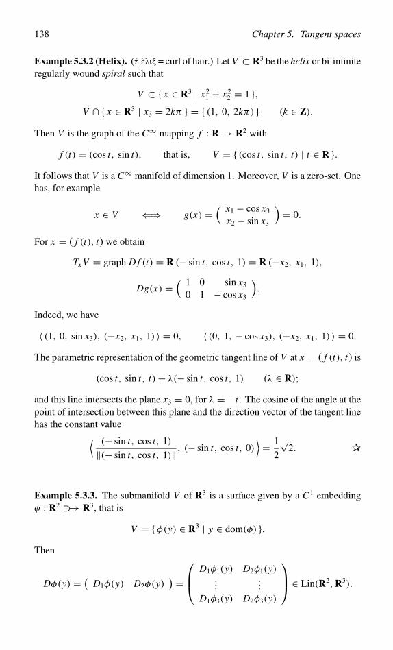
138 Chapter 5. Tangent spaces
Example 5.3.2 (Helix). ( �λιξ = curl of hair.) Let V ⊂ R3 be the helix or bi-infiniteregularly wound spiral such that
V ⊂ { x ∈ R3 | x21 + x2
2 = 1 },V ∩ { x ∈ R3 | x3 = 2kπ } = { (1, 0, 2kπ) } (k ∈ Z).
Then V is the graph of the C∞ mapping f : R → R2 with
f (t) = (cos t, sin t), that is, V = { (cos t, sin t, t) | t ∈ R }.It follows that V is a C∞ manifold of dimension 1. Moreover, V is a zero-set. Onehas, for example
x ∈ V ⇐⇒ g(x) =( x1 − cos x3
x2 − sin x3
)= 0.
For x = ( f (t), t) we obtain
Tx V = graph D f (t) = R (− sin t, cos t, 1) = R (−x2, x1, 1),
Dg(x) =( 1 0 sin x3
0 1 − cos x3
).
Indeed, we have
〈 (1, 0, sin x3), (−x2, x1, 1) 〉 = 0, 〈 (0, 1, − cos x3), (−x2, x1, 1) 〉 = 0.
The parametric representation of the geometric tangent line of V at x = ( f (t), t) is
(cos t, sin t, t)+ λ(− sin t, cos t, 1) (λ ∈ R);and this line intersects the plane x3 = 0, for λ = −t . The cosine of the angle at thepoint of intersection between this plane and the direction vector of the tangent linehas the constant value⟨ (− sin t, cos t, 1)
‖(− sin t, cos t, 1)‖ , (− sin t, cos t, 0)⟩= 1
2
√2. ✰
Example 5.3.3. The submanifold V of R3 is a surface given by a C1 embeddingφ : R2 ⊃→ R3, that is
V = {φ(y) ∈ R3 | y ∈ dom(φ) }.Then
Dφ(y) = (D1φ(y) D2φ(y)
) = D1φ1(y) D2φ1(y)
......
D1φ3(y) D2φ3(y)
∈ Lin(R2,R3).
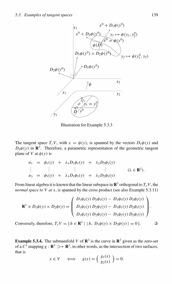
5.3. Examples of tangent spaces 139
y1y0
y1 = y01
D
y 2= y
02
y2x1
φx2
D1φ(y0)D2φ(y0)
D1φ(y0)× D2φ(y0)
y1 �→ φ(y1, y02)
y2 �→ φ(y01 , y2)
x0 = φ(y0)φ(D)
x0 + D1φ(y0)
x0 + D2φ(y0)
x3
Illustration for Example 5.3.3
The tangent space Tx V , with x = φ(y), is spanned by the vectors D1φ(y) andD2φ(y) in R3. Therefore, a parametric representation of the geometric tangentplane of V at φ(y) is
u1 = φ1(y) + λ1 D1φ1(y) + λ2 D2φ1(y)...
......
... (λ ∈ R2).
u3 = φ3(y) + λ1 D1φ3(y) + λ2 D2φ3(y)
From linear algebra it is known that the linear subspace in R3 orthogonal to Tx V , thenormal space to V at x , is spanned by the cross product (see also Example 5.3.11)
R3 � D1φ(y)× D2φ(y) =
D1φ2(y) D2φ3(y)− D1φ3(y) D2φ2(y)
D1φ3(y) D2φ1(y)− D1φ1(y) D2φ3(y)
D1φ1(y) D2φ2(y)− D1φ2(y) D2φ1(y)
.
Conversely, therefore, Tx V = { h ∈ R3 | 〈 h, D1φ(y)× D2φ(y) 〉 = 0 }. ✰
Example 5.3.4. The submanifold V of R3 is the curve in R3 given as the zero-setof a C1 mapping g : R3 ⊃→ R2, in other words, as the intersection of two surfaces,that is
x ∈ V ⇐⇒ g(x) =( g1(x)
g2(x)
)= 0.

140 Chapter 5. Tangent spaces
V2 = {g2(x) = 0}
V1 = {g1(x) = 0}
Tx V1grad g2(x)
grad g1(x)
Tx V2
Illustration for Example 5.3.4
Then
Dg(x) =( Dg1(x)
Dg2(x)
)∈ Lin(R3,R2),
ker (Dg(x)) = { h ∈ R3 | 〈 grad g1(x), h〉 = 〈 grad g2(x), h〉 = 0 }.Thus the tangent space Tx V is seen to be the line in R3 through 0, formed byintersection of the two planes { h ∈ R3 | 〈 grad g1(x), h〉 = 0 } and { h ∈ R3 |〈 grad g2(x), h〉 = 0 }. ✰
Example 5.3.5. The submanifold V of Rn is given as the zero-set of a C1 mappingg : Rn ⊃→ Rn−d , that is (see Theorem 4.7.1.(iii))
V = { x ∈ Rn | x ∈ dom(g), g(x) = 0 }.Then h ∈ Tx V , for x ∈ V , if and only if
D(g)(x)h = 0 ⇐⇒ 〈 grad g1(x), h〉 = · · · = 〈 grad gn−d(x), h〉 = 0.
This once again proves the property from Theorem 2.6.3.(iii), namely that the vectorsgrad gi (x) ∈ Rn are orthogonal to the level set g−1({0}) through x , in the sense thatgrad gi (x) is orthogonal to Tx V , for 1 ≤ i ≤ n − d. Phrased differently,
grad gi (x) ∈ (Tx V )⊥ (1 ≤ i ≤ n − d),
the orthocomplement of Tx V in Rn . Furthermore, dim(Tx V )⊥ = n − dim Tx V =n − d, while the n − d vectors grad g1(x), …, gradn−d(x) are linearly independentby virtue of the fact that g is a submersion at x . As a consequence, (Tx V )⊥ isspanned by these gradient vectors. ✰
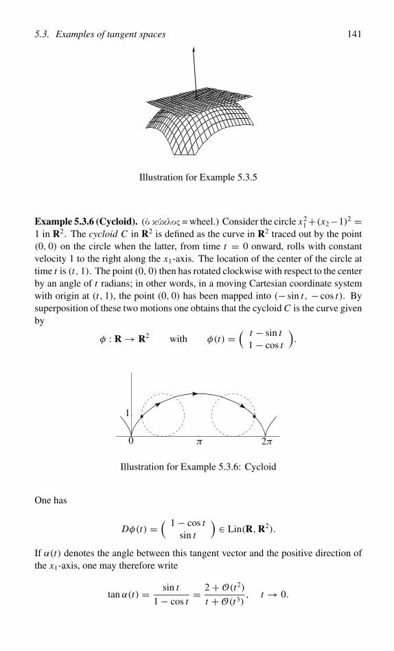
5.3. Examples of tangent spaces 141
Illustration for Example 5.3.5
Example 5.3.6 (Cycloid). (� κ�κλος = wheel.) Consider the circle x21+(x2−1)2 =
1 in R2. The cycloid C in R2 is defined as the curve in R2 traced out by the point(0, 0) on the circle when the latter, from time t = 0 onward, rolls with constantvelocity 1 to the right along the x1-axis. The location of the center of the circle attime t is (t, 1). The point (0, 0) then has rotated clockwise with respect to the centerby an angle of t radians; in other words, in a moving Cartesian coordinate systemwith origin at (t, 1), the point (0, 0) has been mapped into (− sin t, − cos t). Bysuperposition of these two motions one obtains that the cycloid C is the curve givenby
φ : R → R2 with φ(t) =( t − sin t
1− cos t
).
1
0 π 2π
Illustration for Example 5.3.6: Cycloid
One has
Dφ(t) =( 1− cos t
sin t
)∈ Lin(R,R2).
If α(t) denotes the angle between this tangent vector and the positive direction ofthe x1-axis, one may therefore write
tan α(t) = sin t
1− cos t= 2+O(t2)
t +O(t3), t → 0.
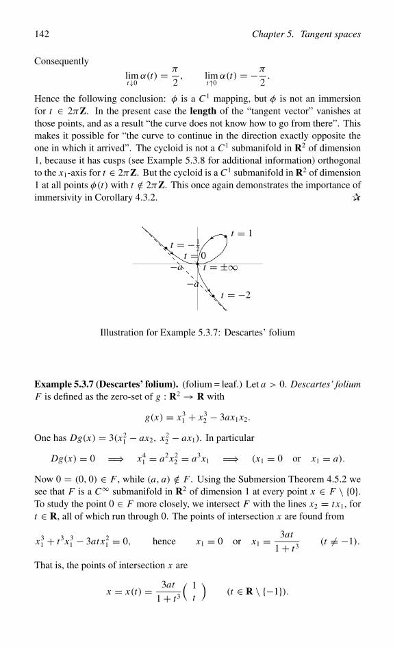
142 Chapter 5. Tangent spaces
Consequently
limt↓0
α(t) = π
2, lim
t↑0α(t) = −π
2.
Hence the following conclusion: φ is a C1 mapping, but φ is not an immersionfor t ∈ 2πZ. In the present case the length of the “tangent vector” vanishes atthose points, and as a result “the curve does not know how to go from there”. Thismakes it possible for “the curve to continue in the direction exactly opposite theone in which it arrived”. The cycloid is not a C1 submanifold in R2 of dimension1, because it has cusps (see Example 5.3.8 for additional information) orthogonalto the x1-axis for t ∈ 2πZ. But the cycloid is a C1 submanifold in R2 of dimension1 at all points φ(t) with t /∈ 2πZ. This once again demonstrates the importance ofimmersivity in Corollary 4.3.2. ✰
−a
−a
t = − 12
t = 0
t = 1
t = ±∞
t = −2
Illustration for Example 5.3.7: Descartes’ folium
Example 5.3.7 (Descartes’ folium). (folium = leaf.) Let a > 0. Descartes’ foliumF is defined as the zero-set of g : R2 → R with
g(x) = x31 + x3
2 − 3ax1x2.
One has Dg(x) = 3(x21 − ax2, x2
2 − ax1). In particular
Dg(x) = 0 =⇒ x41 = a2x2
2 = a3x1 =⇒ (x1 = 0 or x1 = a).
Now 0 = (0, 0) ∈ F , while (a, a) /∈ F . Using the Submersion Theorem 4.5.2 wesee that F is a C∞ submanifold in R2 of dimension 1 at every point x ∈ F \ {0}.To study the point 0 ∈ F more closely, we intersect F with the lines x2 = t x1, fort ∈ R, all of which run through 0. The points of intersection x are found from
x31 + t3x3
1 − 3atx21 = 0, hence x1 = 0 or x1 = 3at
1+ t3(t = −1).
That is, the points of intersection x are
x = x(t) = 3at
1+ t3
( 1t
)(t ∈ R \ {−1}).
5.3. Examples of tangent spaces 143
Therefore im(φ) ⊂ F , with φ : R \ {−1} → R2 given by
φ(t) = 3a
1+ t3
( tt2
).
We have φ(0) = 0, and furthermore
Dφ(t) = 3a
(1+ t3)2
(1+ t3 − 3t3
2t (1+ t3)− 3t4
)= 3a
(1+ t3)2
(1− 2t3
2t − t4
).
In particular
Dφ(0) = 3a( 1
0
).
Consequently, φ is an immersion at the point 0 in R. By the Immersion Theo-rem 4.3.1 it follows that there exists an open neighborhood D of 0 in R such thatφ(D) is a C∞ submanifold of R2 with 0 ∈ φ(D) ⊂ F . Moreover, the tangent lineof φ(D) at 0 is horizontal.
This does not complete the analysis of the structure of F in neighborhoods of0, however. Indeed,
limt→±∞φ(t) = 0 = φ(0),
which suggests that F intersects with itself at 0. Furthermore, the one-parameterfamily of lines { x2 = t x1 | t ∈ R } does not comprise all lines through the origin:it excludes the x2-axis (t = ±∞). Therefore we now intersect F with the linesx1 = ux2, for u ∈ R. We then find the points of intersection
x = x(u) = 3au
1+ u3
( u1
)(u ∈ R \ {−1}).
Therefore im(φ) ⊂ F , with φ : R \ {−1} → R2 given by
φ(u) = 3a
1+ u3
( u2
u
)= φ
(1
u
).
Then
Dφ(u) = 3a
(1+ u3)2
(2u − u4
1− 2u3
), in particular Dφ(0) = 3a
( 01
).
For the same reasons as before there exists an open neighborhood D of 0 in R suchthat φ(D) is a C∞ submanifold of R2 with 0 ∈ φ(D) ⊂ F . However, the tangentline of φ(D) at 0 is vertical.
In summary: F is a C∞ curve at all its points, except at 0; F intersects withitself at 0, in such a way that one part of F at 0 is orthogonal to the other. Thereare two lines that run through 0 in linearly independent directions and that are both“tangent to” F at 0. This makes it plausible that grad g(0) = 0, because grad g(0)must be orthogonal to both “tangent lines” at the same time. ✰
144 Chapter 5. Tangent spaces
Example 5.3.8 (Cusp of a plane curve). Consider the curve γ : R → R2 givenby γ (t) = (t2, t3). The image im(γ ) = { x ∈ R2 | x3
1 = x22 } is said to be the
semicubic parabola (the behavior observed in the parts above and below the x1-axisis like that of a parabola). Note that γ ′(t) = (2t, 3t2)t ∈ Lin(R,R2) is injective,
unless t = 0. Furthermore, ‖γ ′(t)‖ = 2|t |√
1+ ( 32 t)2. For t = 0 we therefore
have the normalized tangent vector
T (t) = ‖γ ′(t)‖−1γ ′(t) = sgn t√1+ ( 3
2 t)2
1
3
2t
.
Obviously, thenlimt↓0
T (t) = (1, 0) = − limt↑0
T (t).
This equality tells us that the unit tangent vector field t �→ T (t) along the curveabruptly reverses its direction at the point 0. We further note that the second deriva-tive γ ′′(0) = (2, 0) and the third derivative γ ′′′(0) = (0, 6) are linearly independentvectors in R2. Finally, C := im(γ ) is not a C1 submanifold in R2 of dimension 1at (0, 0). Indeed, suppose there exist a neighborhood U of (0, 0) in R2 and a C1
function f : W → R with 0 ∈ W , f (0) = 0 and C ∩U = { ( f (w), w) | w ∈ W }.Necessarily, then f (w) = f (−w), for all w ∈ W . But this implies that the tangentspace at (0, 0) of C is the x2-axis, which forms a contradiction.
The reversal of the direction of the unit tangent vector field is characteristic of acusp, and the semicubic parabola is considered the prototype of the simplest typeof cusp (there are also cusps of the form t �→ (t2, t5), etc). If φ : I → R2 is a C3
curve, a possible first definition of an ordinary cusp at a point x0 of φ is that, afterapplication of a local C3 diffeomorphism � of R2 defined in a neighborhood of x0
with �(x0) = (0, 0), the image curve � ◦ φ : I → R2 in a neighborhood of (0, 0)coincides with the curve γ above. Such a definition, however, has the drawbackof not being formulated in terms of the curve φ itself. This is overcome by thefollowing second definition, which can be shown to be a consequence of the firstone. ✰
Definition 5.3.9. Let φ : I → R2 be a C3 curve, 0 ∈ I and φ(0) = x0. Then φ issaid to have an ordinary cusp at x0 if
φ′(0) = 0, and if φ′′(0) and φ′′′(0)
are linearly independent vectors in R2. ❍
Note that for the parabola t �→ (t2, t4) the second and third derivative at 0 arenot linearly independent vectors in R2. It can be proved that Definition 5.3.9 is infact independent of the choice of the parametrization φ. In this book we omit proof
5.3. Examples of tangent spaces 145
of the fact that the second definition is implied by the first one. Instead, we add thefollowing remark. By Taylor expansion we find that for a C4 curve φ : I → R2
with 0 ∈ I , φ(0) = x0 and φ′(0) = 0, the following equality of vectors holds inR2, for t ∈ I :
φ(t) = x0 + t2
2!φ′′(0)+ t3
3!φ′′′(0)+O(t4), t → 0.
If φ satisfies Definition 5.3.9, it follows that
φ(t) = x0 + (t2, t3)+O(t4), t → 0,
which becomes apparent upon application of the linear coordinate transformationin R2 which maps 1
2!φ′′(0) into (1, 0) and 1
3!φ′′′(0) into (0, 1). To prove that the first
definition is a consequence of Definition 5.3.9, one evidently has to show that theterms in t of order higher than 3 can be removed by means of a suitable (nonlinear)coordinate transformation in R2. Also note that the terms of higher order in no wayaffect the reversal of the direction of the unit tangent vector field. Incidentally, theerror is of the order of 1
10.000 for t = 110 , which will go unnoticed in most illustrations.
For practical applications we formulate the following:
Lemma 5.3.10. A curve in R2 has an ordinary cusp at x0 if it possesses a C4
parametrization φ : I → R2 with 0 ∈ I and x0 = φ(0), and if there are numbersa, b ∈ R \ {0} with
φ(t) = x0 +( a t2 +O(t3)
b t3 +O(t4)
), t → 0.
Furthermore, im(φ) at x0 is not a C1 submanifold in R2 of dimension 1.
Proof. 12!φ
′′(0) = (a, 0) and 13!φ
′′′(0) = (∗, b) are linearly independent vectors inR2. The last assertion follows by similar arguments as for the semicubic parabola.❏
By means of this lemma we can once again verify that the cycloid φ : R → R2
from Example 5.3.6 has an ordinary cusp at (0, 0) ∈ R2, and, on account of theperiodicity, at all points of the form (2πk, 0) ∈ R2 for k ∈ Z; indeed, Taylorexpansion gives
φ(t) =( t − sin t
1− cos t
)=
( 16 t3 +O(t4)
12 t2 +O(t3)
), t → 0.
Example 5.3.11 (Hypersurface in Rn). This example will especially be used inChapter 7. Recall that a Ck hypersurface V in Rn is a Ck submanifold of dimension
146 Chapter 5. Tangent spaces
n − 1. For such a hypersurface dim Tx V = n − 1, for all x ∈ V ; and thereforedim(Tx V )⊥ = 1. A normal to V at x is a vector n(x) ∈ Rn with
n(x) ⊥ Tx V and ‖n(x)‖ = 1.
A normal is thus uniquely determined, to within its sign. We now write
Rn � x = (x ′, xn), with x ′ = (x1, . . . , xn−1) ∈ Rn−1.
On account of Theorem 4.7.1 there exists for every x0 ∈ V a neighborhood U of x0
in Rn such that the following assertions are equivalent (this may require permutationof the coordinates of Rn).
(i) There exist an open neighborhood U ′ of (x0)′ in Rn−1 and a Ck functionh : U ′ → R with
V ∩U = graph(h) = { (x ′, h(x ′)) | x ′ ∈ U ′ }.(ii) There exist an open subset D ⊂ Rn−1 and a Ck embedding φ : D → Rn with
V ∩U = im(φ) = {φ(y) | y ∈ D }.(iii) There exists a Ck function g : U → R with Dg(x) = 0 for x ∈ U , such that
V ∩U = N (g, 0) = { x ∈ U | g(x) = 0 }.In Description (i) of V one has, if x = (x ′, h(x ′)),
Tx V = graph (Dh(x ′)) = { (v, Dh(x ′)v) | v ∈ Rn−1 },where
Dh(x ′) = (D1h(x ′), . . . , Dn−1h(x ′)).
Therefore, if e1, . . . , en−1 are the standard basis vectors of Rn−1, it follows that Tx Vis spanned by the vectors u j := (e j , D j h(x ′)), for 1 ≤ j ≤ n − 1. Hence (Tx V )⊥is spanned by the vector w = (w1, . . . , wn−1, 1) ∈ Rn satisfying 0 = 〈w, u j 〉 =w j + D j h(x ′), for 1 ≤ j < n. Therefore w = (−Dh(x ′), 1), and consequently
n(x) = ±(1+ ‖Dh(x ′)‖2)−1/2 (−Dh(x ′), 1) (x = (x ′, h(x ′))).
In Description (iii) one has
Tx V = ker (Dg(x)).
In particular, on the basis of (i) we can choose the function g in (iii) as follows:
g(x) = xn − h(x ′); then Dg(x) = (−Dh(x ′), 1) = 0.
This once again confirms the formula for n(x) given above.In Description (ii) Tx V is spanned by the vectors v j := D jφ(y), for 1 ≤ j < n.
Hence, a vector w ∈ (Tx V )⊥ is determined, to within a scalar, by the equations
〈v j , w〉 = 0 (1 ≤ j < n).
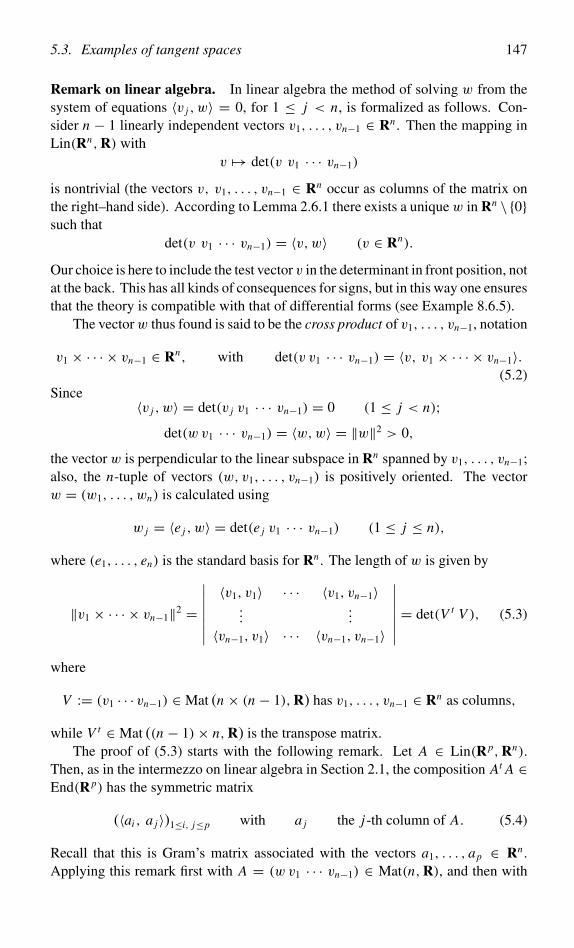
5.3. Examples of tangent spaces 147
Remark on linear algebra. In linear algebra the method of solving w from thesystem of equations 〈v j , w〉 = 0, for 1 ≤ j < n, is formalized as follows. Con-sider n − 1 linearly independent vectors v1, . . . , vn−1 ∈ Rn . Then the mapping inLin(Rn,R) with
v �→ det(v v1 · · · vn−1)
is nontrivial (the vectors v, v1, . . . , vn−1 ∈ Rn occur as columns of the matrix onthe right–hand side). According to Lemma 2.6.1 there exists a unique w in Rn \ {0}such that
det(v v1 · · · vn−1) = 〈v,w〉 (v ∈ Rn).
Our choice is here to include the test vector v in the determinant in front position, notat the back. This has all kinds of consequences for signs, but in this way one ensuresthat the theory is compatible with that of differential forms (see Example 8.6.5).
The vectorw thus found is said to be the cross product of v1, . . . , vn−1, notation
v1 × · · · × vn−1 ∈ Rn, with det(v v1 · · · vn−1) = 〈v, v1 × · · · × vn−1〉.(5.2)
Since〈v j , w〉 = det(v j v1 · · · vn−1) = 0 (1 ≤ j < n);
det(w v1 · · · vn−1) = 〈w,w〉 = ‖w‖2 > 0,
the vector w is perpendicular to the linear subspace in Rn spanned by v1, . . . , vn−1;also, the n-tuple of vectors (w, v1, . . . , vn−1) is positively oriented. The vectorw = (w1, . . . , wn) is calculated using
w j = 〈e j , w〉 = det(e j v1 · · · vn−1) (1 ≤ j ≤ n),
where (e1, . . . , en) is the standard basis for Rn . The length of w is given by
‖v1 × · · · × vn−1‖2 =
∣∣∣∣∣∣∣〈v1, v1〉 · · · 〈v1, vn−1〉
......
〈vn−1, v1〉 · · · 〈vn−1, vn−1〉
∣∣∣∣∣∣∣ = det(V t V ), (5.3)
where
V := (v1 · · · vn−1) ∈ Mat (n × (n − 1),R) has v1, . . . , vn−1 ∈ Rn as columns,
while V t ∈ Mat ((n − 1)× n,R) is the transpose matrix.The proof of (5.3) starts with the following remark. Let A ∈ Lin(Rp,Rn).
Then, as in the intermezzo on linear algebra in Section 2.1, the composition At A ∈End(Rp) has the symmetric matrix
(〈ai , a j 〉)1≤i, j≤p with a j the j-th column of A. (5.4)
Recall that this is Gram’s matrix associated with the vectors a1, . . . , ap ∈ Rn .Applying this remark first with A = (w v1 · · · vn−1) ∈ Mat(n,R), and then with
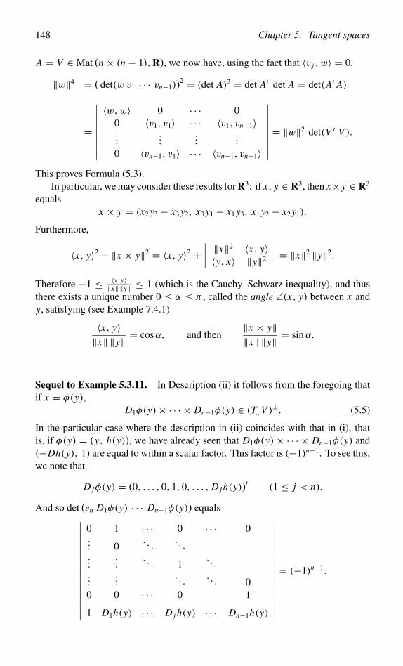
148 Chapter 5. Tangent spaces
A = V ∈ Mat (n × (n − 1),R), we now have, using the fact that 〈v j , w〉 = 0,
‖w‖4 = ( det(w v1 · · · vn−1))2 = (det A)2 = det At det A = det(At A)
=
∣∣∣∣∣∣∣∣∣〈w,w〉 0 · · · 0
0 〈v1, v1〉 · · · 〈v1, vn−1〉...
......
...
0 〈vn−1, v1〉 · · · 〈vn−1, vn−1〉
∣∣∣∣∣∣∣∣∣ = ‖w‖2 det(V t V ).
This proves Formula (5.3).In particular, we may consider these results for R3: if x , y ∈ R3, then x×y ∈ R3
equalsx × y = (x2 y3 − x3 y2, x3 y1 − x1 y3, x1 y2 − x2 y1).
Furthermore,
〈x, y〉2 + ‖x × y‖2 = 〈x, y〉2 +∣∣∣∣ ‖x‖2 〈x, y〉〈y, x〉 ‖y‖2
∣∣∣∣ = ‖x‖2 ‖y‖2.
Therefore −1 ≤ 〈x,y〉‖x‖ ‖y‖ ≤ 1 (which is the Cauchy–Schwarz inequality), and thus
there exists a unique number 0 ≤ α ≤ π , called the angle ∠(x, y) between x andy, satisfying (see Example 7.4.1)
〈x, y〉‖x‖ ‖y‖ = cosα, and then
‖x × y‖‖x‖ ‖y‖ = sin α.
Sequel to Example 5.3.11. In Description (ii) it follows from the foregoing thatif x = φ(y),
D1φ(y)× · · · × Dn−1φ(y) ∈ (Tx V )⊥. (5.5)
In the particular case where the description in (ii) coincides with that in (i), thatis, if φ(y) = (y, h(y)), we have already seen that D1φ(y)× · · · × Dn−1φ(y) and(−Dh(y), 1) are equal to within a scalar factor. This factor is (−1)n−1. To see this,we note that
D jφ(y) = (0, . . . , 0, 1, 0, . . . , D j h(y))t
(1 ≤ j < n).
And so det (en D1φ(y) · · · Dn−1φ(y)) equals∣∣∣∣∣∣∣∣∣∣∣∣∣∣∣∣
0 1 · · · 0 · · · 0... 0
. . .. . .
......
. . . 1. . .
......
. . .. . . 0
0 0 · · · 0 1
1 D1h(y) · · · D j h(y) · · · Dn−1h(y)
∣∣∣∣∣∣∣∣∣∣∣∣∣∣∣∣= (−1)n−1.
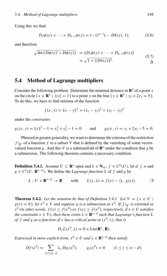
5.4. Method of Lagrange multipliers 149
Using this we find
D1φ(y)× · · · × Dn−1φ(y) = (−1)n−1(− Dh(y), 1); (5.6)
and therefore√det (Dφ(y)t ◦ Dφ(y)) = ‖D1φ(y)× · · · × Dn−1φ(y)‖
= √1+ ‖Dh(y)‖2.
(5.7)✰
5.4 Method of Lagrange multipliers
Consider the following problem. Determine the minimal distance in R2 of a point xon the circle { x ∈ R2 | ‖x‖ = 1 } to a point y on the line { y ∈ R2 | y1+2y2 = 5 }.To do this, we have to find minima of the function
f (x, y) = ‖x − y‖2 = (x1 − y1)2 + (x2 − y2)
2
under the constraints
g1(x, y) = ‖x‖2−1 = x21 + x2
2 −1 = 0 and g2(x, y) = y1+2y2−5 = 0.
Phrased in greater generality, we want to determine the extrema of the restrictionf |V of a function f to a subset V that is defined by the vanishing of some vector-valued function g. And this V is a submanifold of Rn under the condition that g bea submersion. The following theorem contains a necessary condition.
Definition 5.4.1. Assume U ⊂ Rn open and k ∈ N∞, f ∈ Ck(U ); let d ≤ n andg ∈ Ck(U, Rn−d). We define the Lagrange function L of f and g by
L : U × Rn−d → R with L(x, λ) = f (x)− 〈λ, g(x)〉. ❍
Theorem 5.4.2. Let the notation be that of Definition 5.4.1. Let V = { x ∈ U |g(x) = 0 }, let x0 ∈ V and suppose g is a submersion at x0. If f |V is extremal atx0 (in other words, f (x) ≤ f (x0) or f (x) ≥ f (x0), respectively, if x ∈ U satisfiesthe constraint x ∈ V ), then there exists λ ∈ Rn−d such that Lagrange’s function Lof f and g as a function of x has a critical point at (x0, λ), that is
Dx L(x0, λ) = 0 ∈ Lin(Rn,R).
Expressed in more explicit form, x0 ∈ U and λ ∈ Rn−d then satisfy
D f (x0) =∑
1≤i≤n−d
λi Dgi (x0), gi (x
0) = 0 (1 ≤ i ≤ n − d).
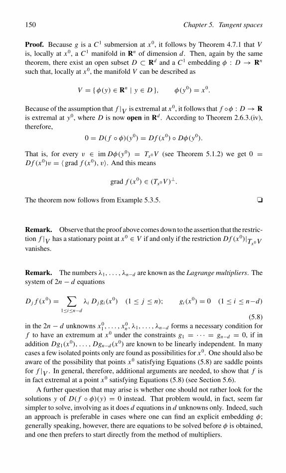
150 Chapter 5. Tangent spaces
Proof. Because g is a C1 submersion at x0, it follows by Theorem 4.7.1 that Vis, locally at x0, a C1 manifold in Rn of dimension d. Then, again by the sametheorem, there exist an open subset D ⊂ Rd and a C1 embedding φ : D → Rn
such that, locally at x0, the manifold V can be described as
V = {φ(y) ∈ Rn | y ∈ D }, φ(y0) = x0.
Because of the assumption that f |V is extremal at x0, it follows that f ◦φ : D → Ris extremal at y0, where D is now open in Rd . According to Theorem 2.6.3.(iv),therefore,
0 = D( f ◦ φ)(y0) = D f (x0) ◦ Dφ(y0).
That is, for every v ∈ im Dφ(y0) = Tx0 V (see Theorem 5.1.2) we get 0 =D f (x0)v = 〈 grad f (x0), v〉. And this means
grad f (x0) ∈ (Tx0 V )⊥.
The theorem now follows from Example 5.3.5. ❏
Remark. Observe that the proof above comes down to the assertion that the restric-tion f |V has a stationary point at x0 ∈ V if and only if the restriction D f (x0)|Tx0 Vvanishes.
Remark. The numbers λ1, . . . , λn−d are known as the Lagrange multipliers. Thesystem of 2n − d equations
D j f (x0) =∑
1≤i≤n−d
λi D j gi (x0) (1 ≤ j ≤ n); gi (x
0) = 0 (1 ≤ i ≤ n−d)
(5.8)in the 2n − d unknowns x0
1 , . . . , x0n , λ1, . . . , λn−d forms a necessary condition for
f to have an extremum at x0 under the constraints g1 = · · · = gn−d = 0, if inaddition Dg1(x0), . . . , Dgn−d(x0) are known to be linearly independent. In manycases a few isolated points only are found as possibilities for x0. One should also beaware of the possibility that points x0 satisfying Equations (5.8) are saddle pointsfor f |V . In general, therefore, additional arguments are needed, to show that f isin fact extremal at a point x0 satisfying Equations (5.8) (see Section 5.6).
A further question that may arise is whether one should not rather look for thesolutions y of D( f ◦ φ)(y) = 0 instead. That problem would, in fact, seem farsimpler to solve, involving as it does d equations in d unknowns only. Indeed, suchan approach is preferable in cases where one can find an explicit embedding φ;generally speaking, however, there are equations to be solved before φ is obtained,and one then prefers to start directly from the method of multipliers.
5.5. Applications of the method of multipliers 151
5.5 Applications of the method of multipliers
Example 5.5.1. We return to the problem from the beginning of Section 5.4. Wediscuss it in a more general context and consider the question: what is the minimaldistance between the unit sphere S = { x ∈ Rn | ‖x‖ = 1 } and the (n − 1)-dimensional linear submanifold L = { y ∈ Rn | 〈y, a〉 = c }, here a ∈ S and c ∈ Rare nonnegative. (Verify that every linear submanifold of dimension n − 1 can berepresented in this form.) Define f : R2n → R and g : R2n → R2 by
f (x, y) = ‖x − y‖2, g(x, y) =( ‖x‖2 − 1
〈y, a〉 − c
).
Application of Theorem 5.4.2 shows that an extremal point (x0, y0) ∈ R2n for therestriction of f to g−1({0}) satisfies the following conditions: there exists λ ∈ R2
such that( 2(x0 − y0)
2(y0 − x0)
)= λ1
( 2x0
0
)+ λ2
( 0a
), and g(x0, y0) = 0.
If λ1 = 0 or λ2 = 0, then x0 = y0, which gives x0 ∈ S∩L; in that case the minimumequals 0. Further, the Cauchy–Schwarz inequality then implies |c| = |〈x0, a〉| ≤‖x0‖ ‖a‖ = 1. From now on we assume c > 1, which implies S ∩ L = ∅. Thenλ1 = 0 and λ2 = 0, and we conclude
x0 = µ a := − λ2
2λ1a and y0 = (1− λ1)µ a.
But g1(x0, y0) = 0 gives µ = ±1 and g2(x0, y0) = 0 gives (1 − λ1)µ = c. Weobtain ‖x0 − y0‖ = ‖ ± a − c a‖ = c ± 1 and so the minimal value equals c − 1.In the problem preceding Definition 5.4.1 we have a = 1√
5(1, 2) and c = √5, the
minimal distance therefore is√
5−1, if we use a geometrical argument to concludethat we actually have a minimum.
Strictly speaking, the reasoning above only shows that c− 1 is a critical value,see the next section for a systematic discussion of this problem. Now we givean argument ad hoc that we have a minimum. We decompose arbitrary elementsx ∈ S and y ∈ L in components along a and perpendicular to a, that is, we writex = α a + v and y = β a + w, where 〈v, a〉 = 〈w, a〉 = 0. From g(x, y) = 0we obtain |α| ≤ 1 and β = c, and accordingly the Pythagorean property fromLemma 1.1.5.(iv) gives
‖x − y‖2 = (α − β)2 + ‖v − w‖2 = (c − α)2 + ‖v − w‖2 ≥ (c − 1)2. ✰
152 Chapter 5. Tangent spaces
Example 5.5.2. Here we generalize the arguments from Example 5.5.1. Let V1 andV2 be C1 submanifolds in R2 of dimension 1. Assume there exist x0
i ∈ Vi with
‖x01 − x0
2‖ = inf / sup{ ‖x1 − x2‖ | xi ∈ Vi (i = 1, 2) },and further assume that, locally at x0
i , the Vi are described by gi (x) = 0, for i = 1, 2.Then f (x1, x2) = ‖x1 − x2‖2 has an extremum at (x0
1 , x02) under the constraints
g1(x1) = g2(x2) = 0. Consequently,
D f (x01 , x0
2) = 2(x01 − x0
2 , −(x01 − x0
2)) = (λ1 Dg1(x01), λ2 Dg2(x
02)).
That is, x01 − x0
2 ∈ R grad g1(x01) = R grad g2(x0
2). In other words (see Theo-rem 5.1.2),
x01 − x0
2 is orthogonal to Tx01V1 and orthogonal to Tx0
2V2. ✰
Example 5.5.3 (Hadamard’s inequality). A parallelepiped has maximal volume(see Example 6.6.3) when it is rectangular. That is, for a j ∈ Rn , with 1 ≤ j ≤ n,
| det(a1 · · · an)| ≤∏
1≤ j≤n
‖a j‖;
and equality obtains if and only if the vectors a j are mutually orthogonal.In fact, consider A := (a1 · · · an) ∈ Mat(n,R), the matrix with the a j as its
column vectors; then a j = Ae j where e j ∈ Rn is the j-th standard basis vector.Note that a proof is needed only in the case where ‖a j‖ = 0; moreover, because themapping A �→ det A is n-linear in the column vectors, we may assume ‖a j‖ = 1,for all 1 ≤ j ≤ n. Now define f j and f : Mat(n,R)→ R by
f j (A) = 1
2(‖a j‖2 − 1), and f (A) = det A.
The problem therefore is to prove that | f (A)| ≤ 1 if f1(A) = . . . = fn(A) = 0.We have D f j (A)H = 〈a j , h j 〉, and therefore
grad f j (A) = (0 · · · 0 a j 0 · · · 0) ∈ Mat(n,R).
Note that the matrices grad f j (A), for 1 ≤ j ≤ n, are linearly independent inMat(n,R). Set A = (ai j ) with
ai j = det(a1 · · · ai−1 e j ai+1 · · · an), and a∗j = (A)t e j ∈ Rn.
The identity a j = Ae j and Cramer’s rule det A · I = A A = AA from (2.6) nowyield
f (A) = det A = 〈a∗j , a j 〉 (1 ≤ j ≤ n). (5.9)
5.5. Applications of the method of multipliers 153
Because the coefficients of A occurring in a j do not occur in a∗j , we obtain (see alsoExercise 2.44.(i))
grad f (A) = (a∗1 a∗2 · · · a∗n) = (A)t ∈ Mat(n,R).
According to Lagrange there exists a λ ∈ Rn such that for the A ∈ Mat(n,R)wheref (A) possibly is extremal, grad f (A) = ∑
1≤ j≤n λ j grad f j (A). We thereforeexamine the following identity of matrices:
(a∗1 a∗2 · · · a∗n) = (λ1a1 λ2a2 · · · λnan), in particular a∗j = λ j a j .
Accordingly, using Formula (5.9) we find that λ j = det A, but applying At to bothsides of the latter identity above and using Cramer’s rule once more then gives
det A e j = det A (At A)e j (1 ≤ j ≤ n).
Therefore there are two possibilities: either det A = 0, which implies f (A) = 0;or At A = I , which implies A ∈ O(n,R) and also f (A) = det A = ±1. Thereforethe absolute maximum of f on { A ∈ Mat(n,R) | f1(A) = · · · = fn(A) = 0 } iseither 0 or ±1, and so we certainly have f (A) ≤ 1 on that set. Now f (I ) = 1,therefore max f = 1; and from the preceding it is evident that A is orthogonal iff (A) = 1. ✰
Remark. In applications one often encounters the following, seemingly moregeneral, problem. Let U be an open subset of Rn and let gi , for 1 ≤ i ≤ p, and hk ,for 1 ≤ k ≤ q, be functions in C1(U ). Define
F = { x ∈ U | gi (x) = 0, 1 ≤ i ≤ p, hk(x) ≤ 0, 1 ≤ k ≤ q }.In other words, F is a subset of an open set defined by p equalities and q inequalities.Again the problem is to determine the extremal values of the restriction of f ∈C1(U ) to F , and if necessary, to locate the extremal points in F . This can bereduced to the problem of finding the extremal values of f under constraints on anopen set as follows. For every subset Q ⊂ Q0 = { 1, . . . , q } define
FQ = { x ∈ U | gi (x) = 0, 1 ≤ i ≤ p, hk(x) = 0, k ∈ Q, hl(x) < 0, l /∈ Q }.Then F is the union of the mutually disjoint sets FQ , for Q running through all thesubsets of Q0. With the notation
UQ = { x ∈ U | hl(x) < 0, l /∈ Q },we see that K Q takes the form, familiar from the method of Lagrange multipliers,
K Q = { x ∈ UQ | gi (x) = 0, 1 ≤ i ≤ p, hk(x) = 0, k ∈ Q }.When f |F attains an extremum at x ∈ FQ , then f |FQ
certainly attains an extremum
at x ; and if applicable, the method of multipliers can now be used to find those pointsx ∈ FQ , for all Q ⊂ Q0. The set of points where the method of multipliers doesnot apply because the gradients are linearly dependent is closed and therefore smallgenerically. These cases should be treated separately.
154 Chapter 5. Tangent spaces
5.6 Closer investigation of critical points
Let the notation be that of Theorem 5.4.2. In the proof of this theorem it is shownthat the restriction f |V has a critical point at x0 ∈ V if and only if the restrictionD f (x0)|Tx0 V vanishes. Our next goal is to define the Hessian of f |V at a criti-
cal punt x0, see Section 2.9, and to use it for the investigation of critical points.We expect it to be a bilinear form on Tx0 V , in other words, to be an element ofLin2(Tx0 V,R), see Definition 2.7.3.
As preparation we choose a local C2 parametrization V ∩ U = im φ with φ :D → Rn according to Theorem 4.7.1, and write x = φ(y). For f ∈ C2(U,R), andφ, the Hessian D2 f (x) ∈ Lin2(Rn,R), and D2φ(y) ∈ Lin2(Rd,Rn), respectively,is well-defined. Differentiating the identity
D( f ◦ φ)(y)w = D f (φ(y))Dφ(y)w (y ∈ D, w ∈ Rd)
with respect to y we find, for v, w ∈ Rd ,
D2( f ◦ φ)(y)(v,w) = D2 f (x)(Dφ(y)v, Dφ(y)w)+ D f (x)D2φ(y)(v,w).(5.10)
Note that D2φ(y)(v,w) ∈ Rn , and that D f (x) does map this vector into R. SinceD2φ(y0)(v,w) does not necessarily belong to Tx0 V , the second term at the right–hand side does not vanish automatically at x0, even though D f (x0)|Tx0 V vanishes.
Yet there exists an expression for the Hessian of f ◦ φ at y0 as a bilinear form onTx0 V .
Definition 5.6.1. From Definition 5.4.1 we recall the Lagrange function L : U ×Rn−d → R of f and g, which satisfies L(x, λ) = f (x) − 〈λ, g(x)〉. ThenD2
x L(x0, λ) ∈ Lin2(Rn,R). The bilinear form
H( f |V )(x0) := D2x L(x0, λ)|Tx0 V ∈ Lin2(Tx0 V,R).
is said to be the Hessian of f |V at x0. ❍
Theorem 5.6.2. Let the notation be that of Theorem 5.4.2, but with k ≥ 2, assumef |V has a critical point at x0, and let λ ∈ Rn−d be the associated Lagrange multi-plier. The definition of H( f |V )(x0) is independent of the choice of the submersiong such that V = g−1({0}). Further, we have, for every C2 embedding φ : D → Rn
with D open in Rd and x0 = φ(y0) ∈ V and every v, w ∈ Tx0 V
H( f |V )(x0)(v,w) = D2( f ◦ φ)(y0)(Dφ(y0)−1v, Dφ(y0)−1w).
Proof. The vanishing of g on V implies that f = L on V , whence f ◦ φ =L ◦ φ on the open set D in Rd . Accordingly we have D2( f ◦ φ)(y0) = D2(L ◦
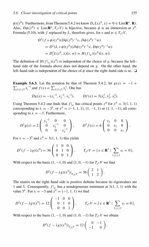
5.6. Closer investigation of critical points 155
φ)(y0). Furthermore, from Theorem 5.4.2 we know Dx L(x0, λ) = 0 ∈ Lin(Rn,R).Also, Dφ(y0) ∈ Lin(Rd, Tx0 V ) is bijective, because φ is an immersion at y0.Formula (5.10), with f replaced by L , therefore gives, for v and w ∈ Tx0 V ,
D2( f ◦ φ)(y0)(Dφ(y0)−1v, Dφ(y0)−1w)
= D2(L ◦ φ)(y0)(Dφ(y0)−1v, Dφ(y0)−1w)
= D2x L(x0, λ)(v,w) = H( f |V )(x0)(v,w).
The definition of H( f |V )(x0) is independent of the choice of g, because the left–hand side of the formula above does not depend on g. On the other hand, theleft–hand side is independent of the choice of φ since the right–hand side is so. ❏
Example 5.6.3. Let the notation be that of Theorem 5.4.2, let g(x) = −1 +∑1≤i≤3 x−1
i and f (x) =∑1≤i≤3 x3
i . One has
Dg(x) = −(x−21 , x−2
2 , x−23 ), D f (x) = 3(x2
1 , x22 , x2
3).
Using Theorem 5.4.2 one finds that f |V has critical points x0 for x0 = 3(1, 1, 1)corresponding to λ = −35, or x0 = (−1, 1, 1), (1,−1, 1) or (1, 1,−1), all corre-sponding to λ = −3. Furthermore,
D2g(x) = 2
x−31 0 00 x−3
2 00 0 x−3
3
, D2 f (x) = 6
x1 0 00 x2 00 0 x3
.
For λ = −35 and x0 = 3(1, 1, 1) this yields
D2( f − λg)(x0) = 36
1 0 00 1 00 0 1
, Tx0 V = { v ∈ R3 |∑
1≤i≤3
vi = 0 }.
With respect to the basis (1,−1, 0) and (1, 0,−1) for Tx0 V we find
D2( f − λg)(x0)|Tx0 V = 36
(2 11 2
).
The matrix on the right–hand side is positive definite because its eigenvalues are1 and 3. Consequently, f |V has a nondegenerate minimum at 3(1, 1, 1) with thevalue 34. For λ = −3 and x0 = (−1, 1, 1) we find
D2( f − λg)(x0) = 12
−1 0 00 1 00 0 1
, Tx0 V = { v ∈ R3 |∑
1≤i≤3
vi = 0 }.
With respect to the basis (1,−1, 0) and (1, 0,−1) for Tx0 V we obtain
D2( f − λg)(x0)|Tx0 V = 12
(0 −1−1 0
).
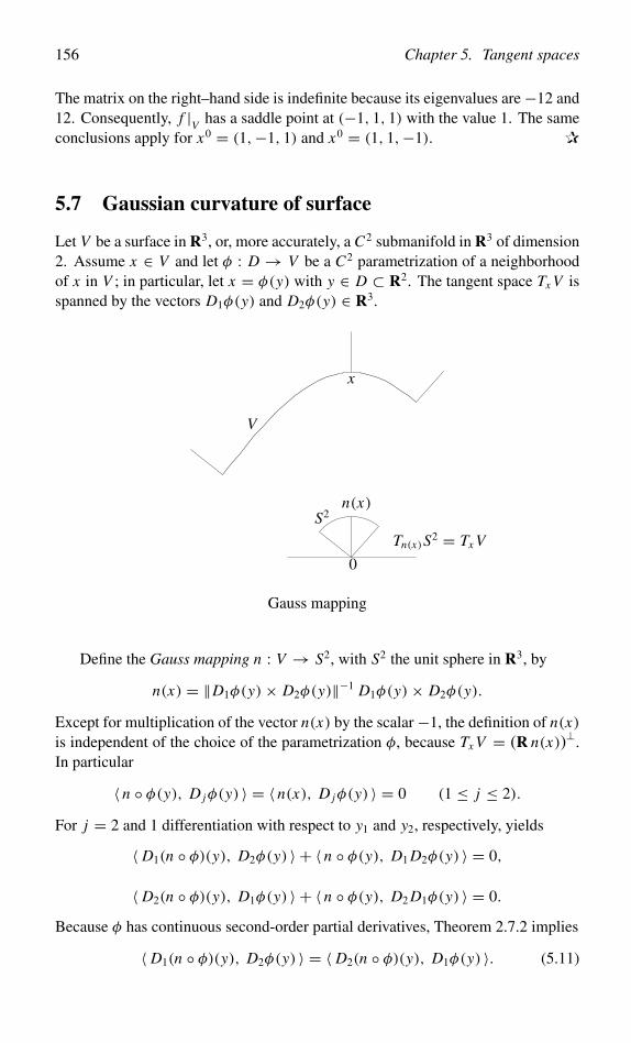
156 Chapter 5. Tangent spaces
The matrix on the right–hand side is indefinite because its eigenvalues are−12 and12. Consequently, f |V has a saddle point at (−1, 1, 1) with the value 1. The sameconclusions apply for x0 = (1,−1, 1) and x0 = (1, 1,−1). ✰
5.7 Gaussian curvature of surface
Let V be a surface in R3, or, more accurately, a C2 submanifold in R3 of dimension2. Assume x ∈ V and let φ : D → V be a C2 parametrization of a neighborhoodof x in V ; in particular, let x = φ(y) with y ∈ D ⊂ R2. The tangent space Tx V isspanned by the vectors D1φ(y) and D2φ(y) ∈ R3.
x
V
S2n(x)
0
Tn(x)S2 = Tx V
Gauss mapping
Define the Gauss mapping n : V → S2, with S2 the unit sphere in R3, by
n(x) = ‖D1φ(y)× D2φ(y)‖−1 D1φ(y)× D2φ(y).
Except for multiplication of the vector n(x) by the scalar−1, the definition of n(x)is independent of the choice of the parametrization φ, because Tx V = (R n(x))⊥.In particular
〈 n ◦ φ(y), D jφ(y) 〉 = 〈 n(x), D jφ(y) 〉 = 0 (1 ≤ j ≤ 2).
For j = 2 and 1 differentiation with respect to y1 and y2, respectively, yields
〈 D1(n ◦ φ)(y), D2φ(y) 〉 + 〈 n ◦ φ(y), D1 D2φ(y) 〉 = 0,
〈 D2(n ◦ φ)(y), D1φ(y) 〉 + 〈 n ◦ φ(y), D2 D1φ(y) 〉 = 0.
Because φ has continuous second-order partial derivatives, Theorem 2.7.2 implies
〈 D1(n ◦ φ)(y), D2φ(y) 〉 = 〈 D2(n ◦ φ)(y), D1φ(y) 〉. (5.11)
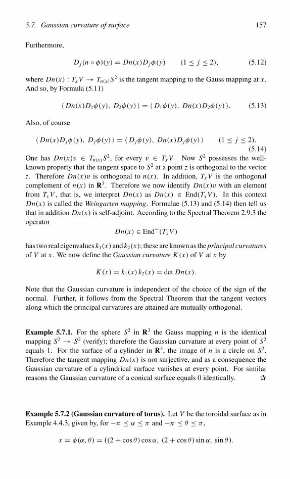
5.7. Gaussian curvature of surface 157
Furthermore,
D j (n ◦ φ)(y) = Dn(x)D jφ(y) (1 ≤ j ≤ 2), (5.12)
where Dn(x) : Tx V → Tn(x)S2 is the tangent mapping to the Gauss mapping at x .And so, by Formula (5.11)
〈 Dn(x)D1φ(y), D2φ(y) 〉 = 〈 D1φ(y), Dn(x)D2φ(y) 〉. (5.13)
Also, of course
〈 Dn(x)D jφ(y), D jφ(y) 〉 = 〈 D jφ(y), Dn(x)D jφ(y) 〉 (1 ≤ j ≤ 2).(5.14)
One has Dn(x)v ∈ Tn(x)S2, for every v ∈ Tx V . Now S2 possesses the well-known property that the tangent space to S2 at a point z is orthogonal to the vectorz. Therefore Dn(x)v is orthogonal to n(x). In addition, Tx V is the orthogonalcomplement of n(x) in R3. Therefore we now identify Dn(x)v with an elementfrom Tx V , that is, we interpret Dn(x) as Dn(x) ∈ End(Tx V ). In this contextDn(x) is called the Weingarten mapping. Formulae (5.13) and (5.14) then tell usthat in addition Dn(x) is self-adjoint. According to the Spectral Theorem 2.9.3 theoperator
Dn(x) ∈ End+(Tx V )
has two real eigenvalues k1(x) and k2(x); these are known as the principal curvaturesof V at x . We now define the Gaussian curvature K (x) of V at x by
K (x) = k1(x) k2(x) = det Dn(x).
Note that the Gaussian curvature is independent of the choice of the sign of thenormal. Further, it follows from the Spectral Theorem that the tangent vectorsalong which the principal curvatures are attained are mutually orthogonal.
Example 5.7.1. For the sphere S2 in R3 the Gauss mapping n is the identicalmapping S2 → S2 (verify); therefore the Gaussian curvature at every point of S2
equals 1. For the surface of a cylinder in R3, the image of n is a circle on S2.Therefore the tangent mapping Dn(x) is not surjective, and as a consequence theGaussian curvature of a cylindrical surface vanishes at every point. For similarreasons the Gaussian curvature of a conical surface equals 0 identically. ✰
Example 5.7.2 (Gaussian curvature of torus). Let V be the toroidal surface as inExample 4.4.3, given by, for −π ≤ α ≤ π and −π ≤ θ ≤ π ,
x = φ(α, θ) = ((2+ cos θ) cosα, (2+ cos θ) sin α, sin θ).
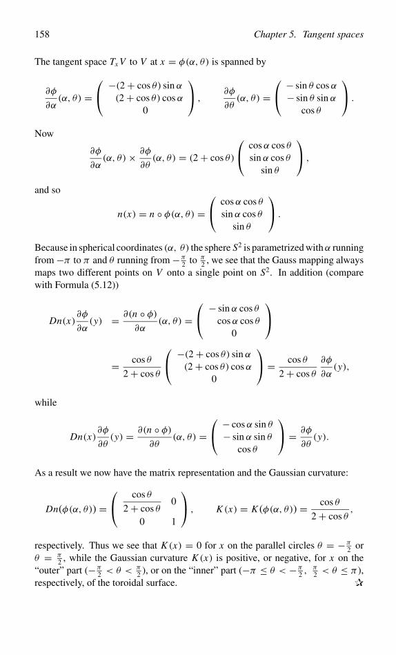
158 Chapter 5. Tangent spaces
The tangent space Tx V to V at x = φ(α, θ) is spanned by
∂φ
∂α(α, θ) =
−(2+ cos θ) sin α(2+ cos θ) cosα
0
,∂φ
∂θ(α, θ) =
− sin θ cosα− sin θ sin α
cos θ
.
Now
∂φ
∂α(α, θ)× ∂φ
∂θ(α, θ) = (2+ cos θ)
cosα cos θsin α cos θ
sin θ
,
and so
n(x) = n ◦ φ(α, θ) = cosα cos θ
sin α cos θsin θ
.
Because in spherical coordinates (α, θ) the sphere S2 is parametrized withα runningfrom−π to π and θ running from−π
2 to π2 , we see that the Gauss mapping always
maps two different points on V onto a single point on S2. In addition (comparewith Formula (5.12))
Dn(x)∂φ
∂α(y) = ∂(n ◦ φ)
∂α(α, θ) =
− sin α cos θcosα cos θ
0
= cos θ
2+ cos θ
−(2+ cos θ) sin α(2+ cos θ) cosα
0
= cos θ
2+ cos θ
∂φ
∂α(y),
while
Dn(x)∂φ
∂θ(y) = ∂(n ◦ φ)
∂θ(α, θ) =
− cosα sin θ− sin α sin θ
cos θ
= ∂φ
∂θ(y).
As a result we now have the matrix representation and the Gaussian curvature:
Dn(φ(α, θ)) = cos θ
2+ cos θ0
0 1
, K (x) = K (φ(α, θ)) = cos θ
2+ cos θ,
respectively. Thus we see that K (x) = 0 for x on the parallel circles θ = −π2 or
θ = π2 , while the Gaussian curvature K (x) is positive, or negative, for x on the
“outer” part (−π2 < θ < π
2 ), or on the “inner” part (−π ≤ θ < −π2 ,
π2 < θ ≤ π),
respectively, of the toroidal surface. ✰
5.8. Curvature and torsion of curve in R3 159
5.8 Curvature and torsion of curve in R3
For a curve in R3 we shall define its curvature and torsion and prove that thesefunctions essentially determine the curve. In this section we need the results onparametrization by arc length from Example 7.4.4.
Definition 5.8.1. Suppose γ : J → Rn is a C3 parametrization by arc length of thecurve im(γ ); in particular, T (s) := γ ′(s) ∈ Rn is a tangent vector of unit lengthfor all s ∈ J . Then the acceleration γ ′′(s) ∈ Rn is perpendicular to im(γ ) at γ (s),as follows by differentiating the identity 〈γ ′(s), γ ′(s)〉 = 1. Accordingly, the unitvector N (s) ∈ Rn in the direction of γ ′′(s) (assuming that γ ′′(s) = 0) is called theprincipal normal to im(γ ) at γ (s), and κ(s) := ‖γ ′′(s)‖ ≥ 0 is called the curvatureof im(γ ) at γ (s). It follows that γ ′′(s) = κ(s)N (s).
Now suppose n = 3. Then define the binormal B(s) ∈ R3 by B(s) := T (s)×N (s), and note that ‖B(s)‖ = 1. Hence (T (s) N (s) B(s)) is a positively orientedtriple of mutually orthogonal unit vectors in R3, in other words, the matrix
O(s) = (T (s) N (s) B(s)) ∈ SO(3,R) (s ∈ J ),
in the notation of Example 4.6.2 and Exercise 2.5.In this context, the following terminology is usual. The linear subspace in R3
spanned by T (s) and N (s) is called the osculating plane (osculum = kiss) of im(γ )
at γ (s), that by N (s) and B(s) the normal plane, and that by B(s) and T (s) therectifying plane. ❍
If we differentiate the identity O(s)t O(s) = I and use (Ot)′ = (O ′)t we find,with O ′(s) = d O
ds (s) ∈ Mat(3,R)
(O(s)t O ′(s))t + O(s)t O ′(s) = 0 (s ∈ J ).
Therefore there exists a mapping J → A(3,R), the linear subspace in Mat(3,R)consisting of antisymmetric matrices, with s �→ A(s) such that
O(s)t O ′(s) = A(s), hence O ′(s) = O(s)A(s) (s ∈ J ). (5.15)
In view of Lemma 8.1.8 we can find a : J → R3 so that we have the followingequality of matrix-valued functions on J :
(T ′ N ′ B ′) = (T N B)
0 −a3 a2
a3 0 −a1
−a2 a1 0
.
In particular, γ ′′ = T ′ = a3 N − a2 B. On the other hand, γ ′′ = κN , and thisimplies κ = a3 and a2 = 0. We write τ(s) := a1(s), the torsion of im(γ ) at γ (s).
160 Chapter 5. Tangent spaces
It follows that a = τT + κB. We now have obtained the following formulae ofFrenet–Serret, with X equal to T , N and B : J → R3, respectively:
(T ′ N ′ B ′) = (T N B)
0 −κ 0κ 0 −τ0 τ 0
,
thus X ′ = a × X,T ′ = κNN ′ = −κT + τ BB ′ = −τN
In particular, if im(γ ) is a planar curve (that is, lies in some plane), then B isconstant, thus B ′ = 0, and this implies τ = 0.
Next we drop the assumption that γ : I → R3 is a parametrization by arclength, that is, we do not necessarily suppose ‖γ ′‖ = 1. Instead, we assume γ tobe a biregular C3 parametrization, meaning that γ ′(t) and γ ′′(t) ∈ R3 are linearlyindependent for all t ∈ I . We shall express T , N , B, κ and τ all in terms of thevelocity γ ′, the speed v := ‖γ ′‖, the acceleration γ ′′, and its derivative γ ′′′. FromExample 7.4.4 we get ds
dt (t) = v(t) if s = λ(t) denotes the arc-length function, andtherefore we obtain for the derivatives with respect to t ∈ I , using the formulae ofFrenet–Serret,
γ ′ = vT,
γ ′′ = v′T + vT ′ = v′T + vdT
ds
ds
dt= v′T + v2κN ,
γ ′ × γ ′′ = v3κT × N = v3κB.
(5.16)
This implies
T = 1
‖γ ′‖γ′, B = 1
‖γ ′ × γ ′′‖γ′ × γ ′′, N = B × T,
κ = ‖γ′ × γ ′′‖‖γ ′‖3
, τ = det(γ ′ γ ′′ γ ′′′)‖γ ′ × γ ′′‖2
.
(5.17)
Only the formula for the torsion τ still needs a proof. Observe that γ ′′′ = (v′T +v2κN )′. The contribution to γ ′′′ that involves B comes from evaluating
v2κN ′ = v3κd N
ds= v3κ(τ B − κT ).
It follows that (γ ′ γ ′′ γ ′′′) is an upper triangular matrix with respect to the basis(T, N , B); and this implies that its determinant equals the product of the coefficientson the main diagonal. Using (5.16) we therefore derive the desired formula:
det(γ ′ γ ′′ γ ′′′) = v6κ2τ = τ‖γ ′ × γ ′′‖2.
5.8. Curvature and torsion of curve in R3 161
Example 5.8.2. For the helix im(γ ) from Example 5.3.2 with γ : R → R3 givenby γ (t) = (a cos t, a sin t, bt) where a > 0 and b ∈ R, we obtain the constantvalues
κ = a
a2 + b2, τ = b
a2 + b2.
If b = 0, the helix reduces to a circle of radius a and its curvature reduces to 1a . It is
a consequence of the following theorem that the only curves with constant, nonzerocurvature and constant, arbitrary torsion are the helices.
Now suppose that γ is a biregular C3 parametrization by arc length s for whichthe ratio of torsion to curvature is constant. Then there exists 0 < α < π with(κ cosα − τ sin α)N = 0. Integrating this equality with respect to the variable sand using the Frenet–Serret formulae we obtain the existence of a fixed unit vectorc ∈ R3 with
cosα T + sin α B = c, whence 〈N , c〉 = 0.
Integrating this once again we find 〈T, c〉 = cosα. That is, the tangent line to im(γ )
makes a constant angle with a fixed vector in R3. In particular, helices have thisproperty (compare with Example 5.3.2). ✰
Theorem 5.8.3. Consider two curves with biregular C3 parametrizations γ1 andγ2 by arc length, both of which have the same curvature and torsion. Then one ofthe curves can be rotated and translated so as to coincide exactly with the other.
Proof. We may assume that the γi : J → R3 for 1 ≤ i ≤ 2 are parametrizationsby arc length s both starting at s0. We have O ′
i = Oi Ai , but the Ai : J → A(3,R)associated with both curves coincide, being in terms of the curvature and torsion.Define C = O2 O−1
1 : J → SO(3,R), thus O2 = C O1. Differentiation withrespect to the arc length s gives
O2 A = O ′2 = C ′O1 + C O1 A = C ′O1 + O2 A, so C ′O1 = 0.
Hence C ′ = 0, and therefore C is a constant mapping. From O2 = C O1 we obtainby considering the first column vectors
γ ′2 = T2 = CT1 = Cγ ′1, therefore γ2(s) = C γ1(s)+ d (s ∈ J ),
with the rotation C ∈ SO(3,R) (see Exercise 2.5) and the vector d ∈ R3 bothconstant. ❏
162 Chapter 5. Tangent spaces
Remark. Let V be a C2 submanifold in R3 of dimension 2 and let n : V → S2
be the corresponding Gauss mapping. Suppose 0 ∈ J and γ : J → R3 is a C2
parametrization by arc length of the curve im(γ ) ⊂ V . We now make a few remarkson the relation between the properties of the Gauss mapping n and the curvature κof γ .
Suppose x = γ (0) ∈ V , then n(x) is a choice of the normal to V at x . Ifγ ′′(0) = 0, let N (0) be the principal normal to im(γ ) at x . Then we define thenormal curvature kn(x) ∈ R of im(γ ) in V at x as
kn(x) = κ(0) 〈n(x), N (0)〉.From 〈(n ◦ γ )(s), T (s)〉 = 0, for s near 0, we find
〈(n ◦ γ )′(s), T (s)〉 + 〈(n ◦ γ )(s), κ(s)N (s)〉 = 0,
and this implies, if v = T (0) = γ ′(0) ∈ Tx V ,
−〈Dn(x)v, v〉 = −〈(n ◦ γ )′(0), T (0)〉 = κ(0) 〈n(x), N (0)〉 = kn(x).
It follows that all curves lying on the surface V and having the same unit tangentvector v at x have the same normal curvature at x . This allows us to speak ofthe normal curvature of V at x along a tangent vector at x . Given a unit vectorv ∈ Tx V , the intersection of V with the plane through x which is spanned by n(x)and v is called the normal section of V at x along v. In a neighborhood of x , anormal section of V at x is an embedded plane curve on V that can be parametrizedby arc length and whose principal normal N (0) at x equals ±n(x) or 0. With thisterminology, we can say that the absolute value of the normal curvature of V at xalong v ∈ Tx V is equal to the curvature of the normal section of V at x along v. Wenow see that the two principal curvatures k1(x) and k2(x) of V at x are the extremevalues of the normal curvature of V at x .
5.9 One-parameter groups and infinitesimal generators
In this section we deal with some theory, which in addition may serve as backgroundto Exercises 2.41, 2.50, 4.22, 5.58 and 5.60. Example 2.4.10 is a typical example ofthis theory. A one-parameter group or group action of C1 diffeomorphisms (�t)t∈R
of Rn is defined as a C1 mapping
� : R×Rn → Rn with �t(x) := �(t, x) ((t, x) ∈ R×Rn), (5.18)
with the property
�0 = I and �t ◦�t ′ = �t+t ′ (t, t ′ ∈ R). (5.19)
It then follows that, for every t ∈ R, the mapping �t : Rn → Rn is a C1 diffeo-morphism, with inverse �−t ; that is
(�t)−1 = �−t (t ∈ R). (5.20)
5.9. One-parameter groups and their generators 163
Note that, for every x ∈ Rn , the curve t �→ �t(x) = �(t, x) : R → Rn isdifferentiable on R, and �0(x) = x . The set {�t(x) | t ∈ R } is said to be the orbitof x under the action of (�t)t∈R.
Next, we define the infinitesimal generator or tangent vector field of the one-parameter group of diffeomorphisms (�t)t∈R on Rn as the mapping φ : Rn → Rn
with
φ(x) = ∂�
∂t(0, x) ∈ Lin(R,Rn) � Rn (x ∈ Rn). (5.21)
By means of Formula (5.19) we find, for (t, x) ∈ R × Rn ,
d
dt�t(x) = d
ds
∣∣∣∣s=0
�s+t(x) = d
ds
∣∣∣∣s=0
�s(�t(x)) = φ(�t(x)). (5.22)
In other words, for every x ∈ Rn the curve t �→ �t(x) is an integral curve γ of theordinary differential equation on Rn , with initial condition respectively
γ ′(t) = φ(γ (t)) (t ∈ R), γ (0) = x . (5.23)
Conversely, the mapping �t is known as the flow over time t of the vector fieldφ. In the theory of differential equations one studies the problem to what extentit is possible, under reasonable conditions on the vector field φ, to construct theone-parameter group (�t)t∈R of flows, starting from φ, and to what extent (�t)t∈R
is uniquely determined by φ. This is complicated by the fact that �t cannot alwaysbe defined for all t ∈ R. In addition, one often deals with the more general problem
γ ′(t) = φ(t, γ (t)),
where the vector fieldφ itself now also depends on the time variable t . To distinguishbetween these situations, the present case of a time-independent vector field is calledautonomous.
We introduce the induced action of (�t)t∈R on C∞(Rn) by assigning �t f ∈C∞(Rn) to �t and f ∈ C∞(Rn), where
(�t f )(x) = f (�−t(x)) (x ∈ Rn). (5.24)
Here we apply the rule: “the value of the transformed function at the transformedpoint equals the value of the original function at the original point”. We then havea group action, that is
(�t�t ′) f = �t(�t ′ f ) (t, t ′ ∈ R, f ∈ C∞(Rn)).
At a more fundamental level even, one identifies a function f : X → R withgraph( f ) ⊂ X × R. Accordingly, the natural definition of the function g = � f :Y → R, for a bijection � : X → Y , is via graph(g) := (� × I ) graph( f ). Thisgives
(y, g(y)) = (�(x), f (x)), hence � f (y) = g(y) = f (x) = f (�−1(y)).
164 Chapter 5. Tangent spaces
Note that in general the action of �t on Rn is nonlinear, that is, one does notnecessarily have �t(x + x ′) = �t(x) + �t(x ′), for x , x ′ ∈ Rn . In contrast, theinduced action of�t on C∞(Rn) is linear; indeed,�t( f +λ f ′) = �t( f )+λ�t( f ′),because ( f + λ f ′)(�−t(x)) = f (�−t(x)) + λ f ′(�−t(x)), for f , f ′ ∈ C∞(Rn),λ ∈ R, x ∈ Rn . On the other hand, Rn is finite-dimensional, while C∞(Rn) isinfinite-dimensional.
In its turn the definition in (5.24) leads to the induced action ∂φ on C∞(Rn) ofthe infinitesimal generator φ of (�t)t∈R, given by
∂φ ∈ End (C∞(Rn)) with (∂φ f )(x) = d
dt
∣∣∣∣t=0
(�t f )(x). (5.25)
This said, from Formulae (5.24) and (5.21) readily follows
(∂φ f )(x) = d
dt
∣∣∣∣t=0
f (�−t(x)) = −D f (x)φ(x) = −∑
1≤ j≤n
φ j (x) D j f (x).
We see that ∂φ is a partial differential operator with variable coefficients on C∞(Rn),with the notation
∂φ(x) = −∑
1≤ j≤n
φ j (x) D j . (5.26)
Note that, but for the−sign, ∂φ(x) is the directional derivative in the direction φ(x).Warning: most authors omit the −sign in this identification of tangent vector fieldand partial differential operator.
Example 5.9.1. Let � : R × R2 → R2 be given by
�(t, x) = (x1 cos t − x2 sin t, x1 sin t + x2 cos t),
that is, �t =( cos t − sin t
sin t cos t
)∈ Mat(2,R).
It readily follows that we have a one-parameter group of diffeomorphisms of R2. Theorbits are the circles in R2 of center 0 and radius≥ 0. Moreover, φ(x) = (−x2, x1).The said circles do in fact satisfy the differential equation(
γ ′1(t)γ ′2(t)
)=
( −γ2(t)γ1(t)
)(t ∈ R).
By means of Formula (5.26) we find ∂φ(x) = x2 D1 − x1 D2, for x ∈ R2. ✰
Example 5.9.2. See Exercise 2.50. Let a ∈ Rn be fixed, and define � : R×Rn →Rn by �(t, x) = x + ta, hence
φ(x) = a, and so ∂φ(x) = −∑
1≤ j≤n
a j D j (x ∈ Rn).
5.9. One-parameter groups and their generators 165
In this case the orbits are straight lines. Further note that ∂φ is a partial differentialoperator with constant coefficients, which we encountered in Exercise 2.50.(ii)under the name ta . ✰
Example 5.9.3. See Example 2.4.10 and Exercises 2.41, 4.22, 5.58 and 5.60. Con-sider a ∈ R3 with‖a‖ = 1, and let�a : R×R3 → R3 be given by�a(t, x) = Rt,a x ,as in Exercise 4.22. It is evident that we then find a one-parameter group in SO(3,R).The orbit of x ∈ R3 is the circle in R3 of center 〈x, a〉 a and radius ‖a × x‖, lyingin the plane through x and orthogonal to a. Using Euler’s formula from Exer-cise 4.22.(iii) we obtain
φa(x) = a × x =: ra(x).
Therefore the orbit of x is the integral curve through x of the following differentialequation for the rotations Rt,a:
d Rt,a
dt(x) = ra ◦ Rt,a(x) (t ∈ R), R0,a(x) = I. (5.27)
According to Formula (5.26) we have
∂φa (x) = 〈a, (grad)× x 〉 = 〈a, L(x) 〉 (x ∈ R3).
Here L is the angular momentum operator from Exercises 2.41 and 5.60. In Exer-cise 5.58 we verify again that the solution of the differential equation (5.27) is givenby Rt, a = et ra , where the exponential mapping is defined as in Example 2.4.10.✰
Finally, we derive Formula (5.31) below, which we shall use in Example 6.6.9.We assume that (�t)t∈R is a one-parameter group of C2 diffeomorphisms. We writeD�t(x) ∈ End(Rn) for the derivative of �t at x with respect to the variable in Rn .Using Formula (5.19) for the first equality below, the chain rule for the second, andthe product rule for determinants for the third, we obtain
d
dtdet D�t(x) = d
ds
∣∣∣∣s=0
det D(�s ◦�t)(x)
= d
ds
∣∣∣∣s=0
det ((D�s)(�t(x)) ◦ (D�t)(x))
= det D�t(x)d
ds
∣∣∣∣s=0
(det ◦D�s)(�t(x)).
(5.28)
Apply the chain rule once again, note that D�0 = DI = I , change the order ofdifferentiation, then use Formula (5.21), and conclude from Exercise 2.44.(i) that(D det)(I ) = tr. This gives
d
ds
∣∣∣∣s=0
(det ◦D�s)(�t(x)) = (D det)(I ) ◦ D( d
ds
∣∣∣∣s=0
�s)(�t(x))
= tr(Dφ)(�t(x)).
(5.29)
166 Chapter 5. Tangent spaces
We now define the divergence of the vector field φ, notation: div φ, as the functionRn → R, with
div φ = tr Dφ =∑
1≤ j≤n
D jφ j . (5.30)
Combining Formulae (5.28) – (5.30) we find
d
dtdet D�t(x) = div φ(�t(x)) det D�t(x) ((t, x) ∈ R × Rn). (5.31)
Because det D�0(x) = 1, solving the differential equation in (5.31) we obtain
det D�t(x) = e∫ t
0 divφ(�τ (x)) dτ ((t, x) ∈ R × Rn). (5.32)
Example 5.9.4. Let A ∈ End(Rn) be fixed, and define � : R × Rn → Rn by�(t, x) = et Ax . According to Example 2.4.10 we thus obtain a one-parametergroup in Aut(Rn), and furthermore we have
φ(x) = Ax, and so ∂φ(x) = −∑
1≤i≤n
( ∑1≤ j≤n
ai j x j
)Di (x ∈ Rn).
Because �t ∈ End(Rn), we have D�t(x) = �t = et A. Moreover, Dφ(x) =A, and so div φ(x) = tr A, for x ∈ Rn . It follows that div φ(�τ(x)) = tr A;consequently, Formula (5.32) gives (compare with Exercise 2.44.(ii))
det(et A) = et tr A (t ∈ R, A ∈ End(Rn)). (5.33)✰
5.10 Linear Lie groups and their Lie algebras
We recall that Mat(n,R) is a linear space, which is linearly isomorphic to Rn2,
and further that GL(n,R) = { A ∈ Mat(n,R) | det A = 0 } is an open subset ofMat(n,R).
Definition 5.10.1. A linear Lie group is a subgroup G of GL(n,R) which is also aC2 submanifold of Mat(n,R). If this is the case, write g = TI G ⊂ Mat(n,R) forthe tangent space of G at I ∈ G. ❍
It is an important result in the theory of Lie groups that the definition above canbe weakened substantially while the same conclusions remain valid, viz., a linearLie group is a subgroup of GL(n,R) that is also a closed subset of GL(n,R), seeExercise 5.64. Further, there is a more general concept of Lie group, but to keepthe exposition concise we restrict ourselves to the subclass of linear Lie groups.
5.10. Linear Lie groups and their Lie algebras 167
According to Example 2.4.10 we have
exp : Mat(n,R)→ GL(n,R), exp X = eX =∑k∈N0
1
k! Xk ∈ GL(n,R).
Then eX1eX2 = eX1+X2 if X1 and X2 ∈ Mat(n,R) commute. We note that γ (t) =et X is a differentiable curve in GL(n,R) with tangent vector at I equal to
γ ′(0) = d
dt
∣∣∣∣t=0
et X = X (X ∈ Mat(n,R)). (5.34)
Because D exp(0) = I ∈ End ( Mat(n,R)), it follows from the Local InverseFunction Theorem 3.2.4 that there exists an open neighborhood of 0 in Mat(n,R)such that the restriction of exp to U is a diffeomorphism onto an open neighborhoodof I in GL(n,R). As another consequence of (5.34) we see, in view of the definitionof tangent space,
g := { X ∈ Mat(n,R) | et X ∈ G, for all t ∈ R with |t | sufficiently small } ⊂ g.
(5.35)
Theorem 5.10.2. Let G be a linear Lie group, with corresponding tangent space g
at I . Then we have the following assertions.
(i) G is a closed subset of GL(n,R).
(ii) The restriction of the exponential mapping to g maps g into G, hence exp :g→ G. In particular,
g = { X ∈ Mat(n,R) | et X ∈ G, for all t ∈ R }.
Proof. (i). Because G is a submanifold of GL(n,R) there exists an open neighbor-hood U of I in GL(n,R) such that G ∩U is a closed subset of U . As x �→ x−1 is ahomeomorphism of GL(n,R), U−1 is also an open neighborhood of I in GL(n,R).It follows that xU−1 is an open neighborhood of x in GL(n,R). Given x in theclosure G of G in GL(n,R), choose y ∈ xU−1∩G; then y−1x ∈ G ∩U = G ∩U ,whence x ∈ G. This implies assertion (i).(ii). G is a submanifold at I , hence, on account of Proposition 5.1.3, there ex-ist an open neighborhood D of 0 in g and a C1 mapping φ : D → G, suchthat φ(0) = I and Dφ(0) equals the inclusion mapping g → Mat(n,R). Sinceexp : Mat(n,R)→ GL(n,R) is a local diffeomorphism at 0, we may adapt D toarrange that there exists a C1 mapping ψ : D → Mat(n,R) with ψ(0) = 0 and
φ(X) = eψ(X) (X ∈ D).
By application of the chain rule we see that Dφ(0) = D exp(0)Dψ(0) = Dψ(0),hence Dψ(0) equals the inclusion map g → Mat(n,R) too. Now let X ∈ g be
168 Chapter 5. Tangent spaces
arbitrary. For k ∈ N sufficiently large we have 1k X ∈ D, which implies φ( 1
k X)k ∈G. Furthermore,
φ(1
kX)k = (
eψ(1k X)
)k = ekψ( 1k X) → eX as k →∞,
since limk→∞ kψ( 1k X) = Dψ(0)X = X by the definition of derivative. Because
G is closed, we obtain eX ∈ G, which implies g ⊂ g, see Formula (5.35). Thisyields the equality g = g = { X ∈ Mat(n,R) | et X ∈ G, for all t ∈ R }. ❏
Example 5.10.3. In terms of endomorphisms of Rn instead of matrices, g =End(Rn) if G = Aut(Rn). Further, Formula (5.33) implies g = sl(n,R) ifG = SL(n,R), where
sl(n,R) = { X ∈ Mat(n,R) | tr X = 0 },SL(n,R) = { A ∈ GL(n,R) | det A = 1 }. ✰
We need some more definitions. Given g ∈ G, we define the mapping
Ad g : G → G by (Ad g)(x) = gxg−1 (x ∈ G).
Obviously Ad g is a C2 diffeomorphism of G leaving I fixed. Next we define, seeDefinition 5.2.1,
Ad g = D(Ad g)(I ) ∈ End(g).
Ad g ∈ End(g) is called the adjoint mapping of g ∈ G. Because gY k g−1 =(gY g−1)k for all g ∈ G, Y ∈ g and k ∈ N, we have Ad g(etY ) = g etY g−1 =et gY g−1
, and therefore, on the strength of Formula (5.34), the chain rule, and Theo-rem 5.10.2.(ii)
(Ad g)Y = d
dt
∣∣∣∣t=0
(Ad g)(etY ) = d
dt
∣∣∣∣t=0
et gY g−1 = gY g−1 ∈ g.
Hence, Ad acts by conjugation, as does Ad. Further, we find, for g, h ∈ G andY ∈ g,
Ad gh = Ad g ◦ Ad h, Ad : G → Aut(g). (5.36)
Ad : G → Aut(g) is said to be the adjoint representation of G in the linear space ofautomorphisms of g. Furthermore, since Ad is a C1 diffeomorphism we can define
ad = D(Ad)(I ) : g→ End(g).
For the same reasons as above we obtain, for all X , Y ∈ g,
(ad X)Y = d
dt
∣∣∣∣t=0
(Ad et X )Y = d
dt
∣∣∣∣t=0
et X Y e−t X = XY − Y X =: [ X, Y ].
Thus we see that g in addition to being a vector space carries the structure of a Liealgebra, which is defined in the following:
5.10. Linear Lie groups and their Lie algebras 169
Definition 5.10.4. A vector space g is said to be a Lie algebra if it is provided witha bilinear mapping g × g → g, called the Lie brackets or commutator, which isanticommutative, and satisfies Jacobi’s identity, for X1, X2 and X3 ∈ g,
[ X1, X2 ] = −[ X2, X1 ],[ X1, [ X2, X3 ] ] + [ X2, [ X3, X1 ] ] + [ X3, [ X1, X2 ] ] = 0. ❍
Therefore we are justified in calling g the Lie algebra of G. Note that Jacobi’sidentity can be reformulated as the assertion that ad X1 satisfies Leibniz’ rule, thatis
(ad X1)[ X2, X3 ] = [ (ad X1)X2, X3 ] + [ X2, (ad X1)X3 ].This property (partially) explains why ad X ∈ End(g) is called the inner derivationdetermined by X ∈ g. (As above, ad is coming from adjoint.) Jacobi’s identity canalso be phrased as
ad[ X1, X2 ] = [ ad X1, ad X2 ] ∈ End(g).
Remark. If the group G is Abelian, or in other words, commutative, then Ad g =I , for all g ∈ G. In turn, this implies ad X = 0, for all X ∈ g, and therefore[ X1, X2 ] = 0 for all X1 and X2 ∈ g in this case. On the other hand, if G isconnected and not Abelian, the Lie algebra structure of g is nontrivial.
At this stage, the Lie algebra g arises as tangent space of the group G, but Liealgebras do occur in mathematics in their own right, without accompanying group.It is a difficult theorem that every finite-dimensional Lie algebra is the Lie algebraof a linear Lie group.
Lemma 5.10.5. Every one-parameter subgroup (�t)t∈R that acts in Rn and con-sists of operators in GL(n,R) is of the form �t = et X , for t ∈ R, where X =d
dt
∣∣∣∣t=0
�t ∈ Mat(n,R), the infinitesimal generator of (�t)t∈R.
Proof. From Formula (5.22) we obtain that �t is an operator-valued solution to theinitial-value problem
d�t
dt= X �t , �0 = I.
According to Example 2.4.10 the unique and globally defined solution to this first-order linear system of ordinary differential equations with constant coefficients isgiven by �t = et X . ❏
With the definitions above we now derive the following results on preservationof structures by suitable mappings. We will see concrete examples of this in, forinstance, Exercises 5.59, 5.60, 5.67.(x) and 5.70.
170 Chapter 5. Tangent spaces
Theorem 5.10.6. Let G and G ′ be linear Lie groups with Lie algebras g and g′,respectively, and let � : G → G ′ be a homomorphism of groups that is of class C1
at I ∈ G. Write φ = D�(I ) : g→ g′. Then we have the following properties.
(i) φ ◦ Ad g = Ad�(g) ◦ φ : g→ g′, for every g ∈ G.
(ii) φ : g→ g′ is a homomorphism of Lie algebras, that is, it is a linear mappingsatisfying in addition
φ([ X1, X2 ]) = [φ(X1), φ(X2) ] (X1, X2 ∈ g).
(iii) � ◦ exp = exp ◦φ : g → G ′. In particular, with � = Ad : G → Aut(g) weobtain Ad ◦ exp = exp ◦ ad : g→ Aut(g).
Accordingly, we have the following commutative diagrams:
g′Ad�g �� g′
g
φ
��
Ad g �� g
φ
�� G� �� G ′
g
exp
��
φ �� g′
exp
�� GAd �� Aut(g)
g
exp
��
ad �� End(g)
exp
��
Proof. (i). Differentiating
�((Ad g)(x)
) = �(gxg−1) = �(g)�(x)�(g)−1 = (Ad�(g)
)(�(x))
with respect to x at x = I in the direction of X2 ∈ g and using the chain rule, weget
(φ ◦ Ad g)X2 = (Ad�(g) ◦ φ)X2.
(ii). Differentiating this equality with respect to g at g = I in the direction ofX1 ∈ g, we obtain the equality in (ii).(iii). The result follows from Theorem 5.10.2.(ii) and Lemma 5.10.5. Indeed, forgiven X ∈ g, both one-parameter groups t �→ �(exp t X) and t �→ exp tφ(X) inG ′ have the same infinitesimal generator φ(X) ∈ g′. ❏
Finally, we give a geometric meaning for the addition and the commutator ing. The sum in g of two vectors each of which is tangent to a curve in G is tangentto the product curve in G, and the commutator in g of tangent vectors is tangent tothe commutator of the curves in G having a modified parametrization.
Proposition 5.10.7. Let G be a linear Lie group with Lie algebra g, and let X andY be in g.
(i) X + Y is the tangent vector at I to the curve R � t �→ et X etY ∈ G.
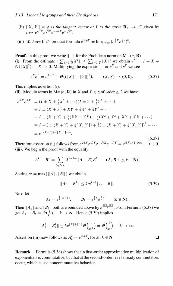
5.10. Linear Lie groups and their Lie algebras 171
(ii) [ X, Y ] ∈ g is the tangent vector at I to the curve R+ → G given byt �→ e
√t X e
√tY e−
√t X e−
√tY .
(iii) We have Lie’s product formula eX+Y = limk→∞ (e1k X e
1k Y )k .
Proof. In this proof we write ‖ · ‖ for the Euclidean norm on Mat(n,R).(i). From the estimate ‖∑k≥2
1k! X
k‖ ≤ ∑k≥2
1k! ‖X‖k we obtain eX = I + X +
O(‖X‖2), X → 0. Multiplying the expressions for eX and eY we see
eX eY = eX+Y +O((‖X‖ + ‖Y‖)2), (X, Y )→ (0, 0). (5.37)
This implies assertion (i).(ii). Modulo terms in Mat(n,R) in X and Y ∈ g of order ≥ 2 we have
e±X e±Y ≡ (I ± X + 12 X2 + · · · )(I ± Y + 1
2 Y 2 + · · · )≡ I ± (X + Y )+ XY + 1
2 X2 + 12 Y 2 + · · ·
= I ± (X + Y )+ 12 (XY − Y X)+ 1
2 (X2 + Y 2 + XY + Y X + · · · )
≡ I + (± (X + Y )+ 12 [ X, Y ])+ 1
2 (± (X + Y )+ 12 [ X, Y ])2 + · · ·
≡ e±(X+Y )+ 12 [ X, Y ]+···.
(5.38)Therefore assertion (ii) follows from e
√t X e
√tY e−
√t X e−
√tY = et[ X, Y ]+o(t), t ↓ 0.
(iii). We begin the proof with the equality
Ak − Bk =∑
0≤l<k
Ak−1−l(A − B)Bl (A, B ∈ g, k ∈ N).
Setting m = max{ ‖A‖, ‖B‖ } we obtain
‖Ak − Bk‖ ≤ kmk−1‖A − B‖. (5.39)
Next letAk = e
1k (X+Y ), Bk = e
1k X e
1k Y (k ∈ N).
Then ‖Ak‖ and ‖Bk‖ both are bounded above by e‖X‖+‖Y‖
k . From Formula (5.37) weget Ak − Bk = O( 1
k2 ), k →∞. Hence (5.39) implies
‖Akk − Bk
k ‖ ≤ ke‖X‖+‖Y‖O( 1
k2
)= O
(1
k
), k →∞.
Assertion (iii) now follows as Akk = eX+Y , for all k ∈ N. ❏
Remark. Formula (5.38) shows that in first-order approximation multiplication ofexponentials is commutative, but that at the second-order level already commutatorsoccur, which cause noncommutative behavior.
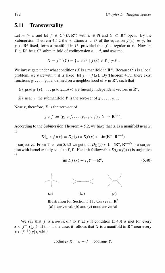
172 Chapter 5. Tangent spaces
5.11 Transversality
Let m ≥ n and let f ∈ Ck(U,Rn) with k ∈ N and U ⊂ Rm open. By theSubmersion Theorem 4.5.2 the solutions x ∈ U of the equation f (x) = y, fory ∈ Rn fixed, form a manifold in U , provided that f is regular at x . Now letY ⊂ Rn be a Ck submanifold of codimension n − d, and assume
X = f −1(Y ) = { x ∈ U | f (x) ∈ Y } = ∅.We investigate under what conditions X is a manifold in Rm . Because this is a localproblem, we start with x ∈ X fixed; let y = f (x). By Theorem 4.7.1 there existfunctions g1, . . . , gn−d , defined on a neighborhood of y in Rn , such that
(i) grad g1(y), . . . , grad gn−d(y) are linearly independent vectors in Rn ,
(ii) near y, the submanifold Y is the zero-set of g1, . . . , gn−d .
Near x , therefore, X is the zero-set of
g ◦ f := (g1 ◦ f, . . . , gn−d ◦ f ) : U → Rn−d .
According to the Submersion Theorem 4.5.2, we have that X is a manifold near x ,if
D(g ◦ f )(x) = Dg(y) ◦ D f (x) ∈ Lin(Rm,Rn−d)
is surjective. From Theorem 5.1.2 we get that Dg(y) ∈ Lin(Rn,Rn−d) is a surjec-tion with kernel exactly equal to TyY . Hence it follows that D(g◦ f )(x) is surjectiveif
im D f (x)+ TyY = Rn. (5.40)
(a) (b) (c)
Illustration for Section 5.11: Curves in R2
(a) transversal, (b) and (c) nontransversal
We say that f is transversal to Y at y if condition (5.40) is met for everyx ∈ f −1({y}). If this is the case, it follows that X is a manifold in Rm near everyx ∈ f −1({y}), while
codimRm X = n − d = codimRn Y.
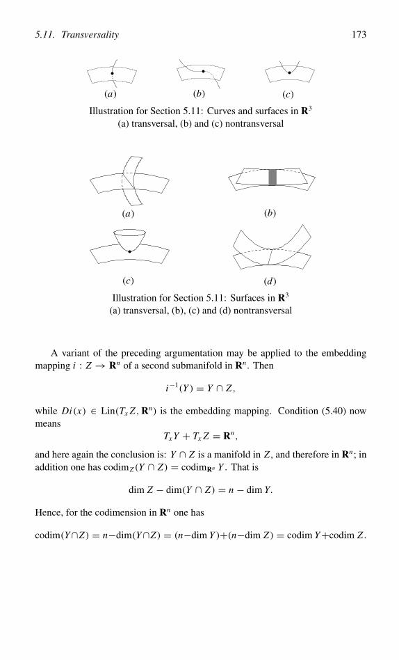
5.11. Transversality 173
(a) (b) (c)
Illustration for Section 5.11: Curves and surfaces in R3
(a) transversal, (b) and (c) nontransversal
(a) (b)
(c) (d)
Illustration for Section 5.11: Surfaces in R3
(a) transversal, (b), (c) and (d) nontransversal
A variant of the preceding argumentation may be applied to the embeddingmapping i : Z → Rn of a second submanifold in Rn . Then
i−1(Y ) = Y ∩ Z ,
while Di(x) ∈ Lin(Tx Z ,Rn) is the embedding mapping. Condition (5.40) nowmeans
Tx Y + Tx Z = Rn,
and here again the conclusion is: Y ∩ Z is a manifold in Z , and therefore in Rn; inaddition one has codimZ (Y ∩ Z) = codimRn Y . That is
dim Z − dim(Y ∩ Z) = n − dim Y.
Hence, for the codimension in Rn one has
codim(Y∩Z) = n−dim(Y∩Z) = (n−dim Y )+(n−dim Z) = codim Y+codim Z .

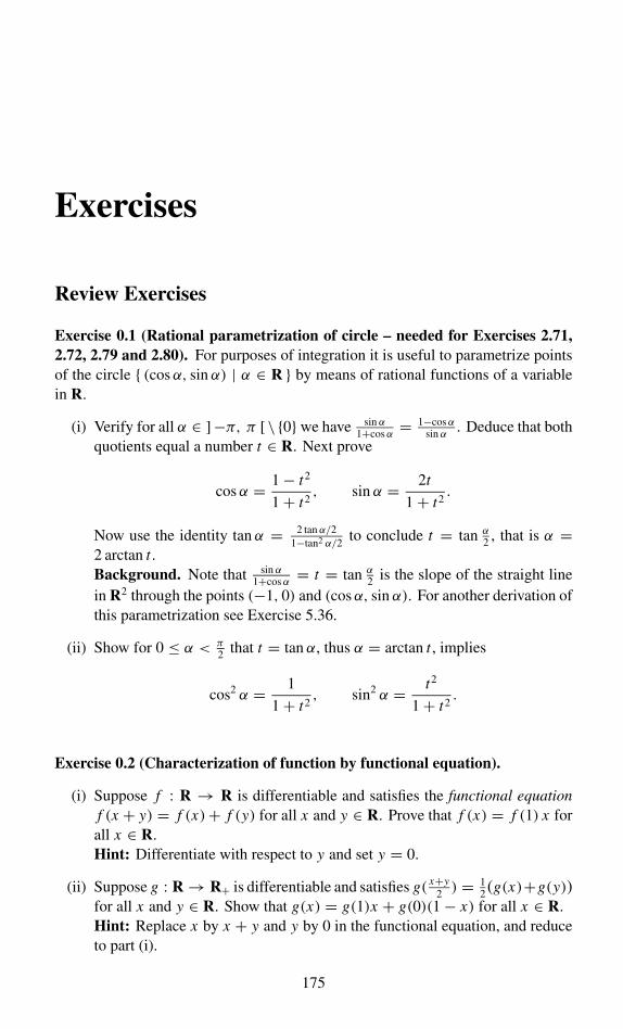
Exercises
Review Exercises
Exercise 0.1 (Rational parametrization of circle – needed for Exercises 2.71,2.72, 2.79 and 2.80). For purposes of integration it is useful to parametrize pointsof the circle { (cosα, sin α) | α ∈ R } by means of rational functions of a variablein R.
(i) Verify for all α ∈ ]−π, π [\ {0}we have sin α1+cosα = 1−cosα
sin α . Deduce that bothquotients equal a number t ∈ R. Next prove
cosα = 1− t2
1+ t2, sin α = 2t
1+ t2.
Now use the identity tan α = 2 tan α/21−tan2 α/2
to conclude t = tan α2 , that is α =
2 arctan t .Background. Note that sin α
1+cosα = t = tan α2 is the slope of the straight line
in R2 through the points (−1, 0) and (cosα, sin α). For another derivation ofthis parametrization see Exercise 5.36.
(ii) Show for 0 ≤ α < π2 that t = tan α, thus α = arctan t , implies
cos2 α = 1
1+ t2, sin2 α = t2
1+ t2.
Exercise 0.2 (Characterization of function by functional equation).
(i) Suppose f : R → R is differentiable and satisfies the functional equationf (x + y) = f (x)+ f (y) for all x and y ∈ R. Prove that f (x) = f (1) x forall x ∈ R.Hint: Differentiate with respect to y and set y = 0.
(ii) Suppose g : R → R+ is differentiable and satisfies g( x+y2 ) = 1
2 (g(x)+g(y))for all x and y ∈ R. Show that g(x) = g(1)x + g(0)(1− x) for all x ∈ R.Hint: Replace x by x + y and y by 0 in the functional equation, and reduceto part (i).
175
176 Review exercises
(iii) Suppose g : R → R+ is differentiable and satisfies g(x + y) = g(x)g(y) forall x and y ∈ R. Show that g(x) = g(1)x for all x ∈ R (see Exercise 6.81for a related result).Hint: Consider f = logg(1) ◦g, where logg(1) is the base g(1) logarithmicfunction.
(iv) Suppose h : R+ → R+ is differentiable and satisfies h(xy) = h(x)h(y) forall x and y ∈ R+. Verify that h(x) = x log h(e) = xh′(1) for all x ∈ R+.Hint: Consider g = h ◦ exp, that is, g(y) = h(ey).
(v) Suppose k : R+ → R is differentiable and satisfies k(xy) = k(x)+ k(y) forall x and y ∈ R+. Show that k(x) = k(e) log x = logb x for all x ∈ R+,where b = ek(e)−1
.Hint: Consider f = k ◦ exp or h = exp ◦k.
(vi) Let f : R → R be Riemann integrable over every closed interval in R andsuppose f (x + y) = f (x) + f (y) for all x and y ∈ R. Verify that theconclusion of (i) still holds.Hint: Integration of f (x + t) = f (x) + f (t) with respect to t over [ 0, y ]gives ∫ y
0f (x + t) dt = y f (x)+
∫ y
0f (t) dt.
Substitution of variables now implies∫ x+y
0f (t) dt =
∫ x
0f (t) dt+
∫ x+y
xf (t) dt =
∫ x
0f (t) dt+
∫ y
0f (x+t) dt.
Hence
y f (x) =∫ x+y
0f (t) dt −
∫ x
0f (t) dt −
∫ y
0f (t) dt.
The technique from part (i) allows us to handle more complicated functional equa-tions too.
(vii) Suppose f : R → R∪{±∞} is differentiable where real-valued and satisfies
f (x + y) = f (x)+ f (y)
1− f (x) f (y)(x, y ∈ R)
where well-defined. Check that f (x) = tan ( f ′(0) x) for x ∈ R withf ′(0)x /∈ π
2 + πZ. (Note that the constant function f (x) = i satisfiesthe equation if we allow complex-valued solutions.)
(viii) Suppose f : R → R is differentiable and satisfies | f (x)| ≤ 1 for all x ∈ Rand
f (x + y) = f (x)√
1− f (y)2 + f (y)√
1− f (x)2 (x, y ∈ R).
Prove that f (x) = sin ( f ′(0)x) for x ∈ R.
Review exercises 177
Exercise 0.3 (Needed for Exercise 3.20). We have
arctan x + arctan1
x=
π
2, x > 0;
−π2, x < 0.
Prove this by means of the following four methods.
(i) Set arctan x = α and express 1x in terms of α.
(ii) Use differentiation.
(iii) Recall that arctan x = ∫ x0
11+t2 dt , and make a substitution of variables.
(iv) Use the formula arctan x + arctan y = arctan ( x+y1−xy ), for x and y ∈ R with
xy = 1, which can be deduced from Exercise 0.2.(vii).
Deduce limx→∞ x(π2 − arctan x) = 1.
Exercise 0.4 (Legendre polynomials and associated Legendre functions – neededfor Exercises 3.17 and 6.63). Let l ∈ N0. The polynomial f (x) = (x2 − 1)l sat-isfies the following ordinary differential equation, which gives a relation amongvarious derivatives of f :
(�) (x2 − 1) f ′(x)− 2lx f (x) = 0.
Define the Legendre polynomial Pl on R by Rodrigues’ formula
Pl(x) = 1
2l l!( d
dx
)l(x2 − 1)l .
(i) Prove by (l + 1)-fold differentiation of (�) that Pl satisfies the following,known as Legendre’s equation for a twice differentiable function u : R → R:
(1− x2) u′′(x)− 2x u′(x)+ l(l + 1) u(x) = 0.
Let m ∈ N0 with m ≤ l.
(ii) Prove by m-fold differentiation of Legendre’s equation that dm Pldxm satisfies the
differential equation
(1− x2) v′′(x)− 2(m + 1)x v′(x)+ (l(l + 1)− m(m + 1)) v(x) = 0.
Now define the associated Legendre function Pml : [ −1, 1 ] → R by
Pml (x) = (1− x2)
m2
dm Pl
dxm(x).
178 Review exercises
(iii) Verify that Pml satisfies
d
dx
((1− x2)
dw
dx(x)
)+
(l(l + 1)− m2
1− x2
)w(x) = 0.
Note that in the case m = 0 this reduces to Legendre’s equation.
(iv) Demonstrate that
d Pml
dx(x) = 1√
1− x2Pm+1
l (x)− mx
1− x2Pm
l (x).
Verify
Pml (x) =
(−1)m
2l l!(l + m)!(l − m)!(1− x2)−
m2
( d
dx
)l−m(x2 − 1)l,
and use this to derive
d Pml
dx(x) = −(l + m)(l − m + 1)√
1− x2Pm−1
l (x)+ mx
1− x2Pm
l (x).
Exercise 0.5 (Parametrization of circle and hyperbola by area). Let e1 =(1, 0) ∈ R2.
(i) Prove that 12 t is the area of the bounded part of R2 bounded by the half-
line R+e1, the unit circle { x ∈ R2 | x21 + x2
2 = 1 }, and the half-lineR+(cos t, sin t), if 0 ≤ t ≤ 2π .
(ii) Prove that 12 t is the area of the bounded part of R2 bounded by R+e1, the branch
{ x ∈ R2 | x21−x2
2 = 1, x1 > 0 }of the unit hyperbola, and R+(cosh t, sinh t),if t ∈ R.
Exercise 0.6 (Needed for Exercise 6.108). Finding antiderivatives for a functionby means of different methods may lead to seemingly distinct expressions for theseantiderivatives. For a striking example of this phenomenon, consider
I =∫
dx√(x − a)(b − x)
(a < x < b).
(i) Compute I by completing the square in the function x �→ (x − a)(b − x).
(ii) Compute I by means of the substitution x = a cos2 θ + b sin2 θ , for 0 < θ <π2 .
(iii) Compute I by means of the substitution b−xx−a = t2, for 0 < t <∞.
Review exercises 179
(iv) Show that for a suitable choice of the constants c1, c2 and c3 ∈ R we have,for all x with a < x < b,
arcsin(2x − b − a
b − a
)+ c1 = arccos
(b + a − 2x
b − a
)+ c2
= −2 arctan
√b − x
x − a+ c3.
Express two of the constants in the third, for instance by substituting x = b.
(v) Show that the following improper integral is convergent, and prove∫ b
a
dx√(x − a)(b − x)
= π.
Exercise 0.7 (Needed for Exercises 3.10, 5.30 and 5.31). Show∫1
cosαdα =
∫cosα
1− sin2 αdα = 1
2log
∣∣∣1+ sin α
1− sin α
∣∣∣+ c.
Use cos 2α = 2 cos2 α − 1 = 1− 2 sin2 α to prove∫1
cosαdα = log
∣∣∣ tan(α
2+ π
4
)∣∣∣+ c.
The number tan(α2 + π4 ) arises in trigonometry also as follows. The triangle in R2
with vertices (0, 0), (0, 1) and (cosα, sin α) is isosceles. This implies that the lineconnecting (0, 1) and (cosα, sin α) has x1-intercept equal to tan(α2 + π
4 ).
Exercise 0.8 (Needed for Exercises 6.60 and 7.30). For p ∈ R+ and q ∈ R,deduce from ∫
R+e(−p+iq)x dx = p + iq
p2 + q2
that ∫R+
e−px cos qx dx = p
p2 + q2,
∫R+
e−px sin qx dx = q
p2 + q2.
Exercise 0.9 (Needed for Exercise 8.21). Let a and b ∈ R with a > |b| and n ∈ N,and prove∫ π
0(a + b cos x)−n dx = (a2 − b2)
12−n
∫ π
0(a − b cos y)n−1 dy.
Hint: Introduce the new variable y by means of
(a+b cos x)(a−b cos y) = a2−b2; use sin x = (a2−b2)12
sin y
a − b cos y.
180 Review exercises
Exercise 0.10 (Duplication formula for (lemniscatic) sine). Set I = [ 0, 1 ].(i) Let α ∈ [ 0, π
4 ], write x = sin α ∈ [ 0, 12
√2 ] and f (x) = sin 2α. Deduce
for x ∈ [ 0, 12
√2 ] that f (x) = 2x
√1− x2 ∈ I and∫ f (x)
0
1√1− t2
dt = 2∫ x
0
1√1− t2
dt.
(ii) Prove that the mapping ψ1 : I → I is an order-preserving bijection ifψ1(u) = 2u2
1+u4 . Verify that the substitution of variables t2 = ψ1(u) yields∫ z
0
1√1− t4
dt = √2∫ y
0
1√1+ u4
du,
where for all y ∈ I we define z ∈ I by z2 = ψ1(y).
(iii) Prove that the mapping ψ2 : [ 0,√√
2− 1 ] → I is an order-preservingbijection ifψ2(t) = 2t2
1−t4 . Verify that the substitution of variables u2 = ψ2(t)yields ∫ y
0
1√1+ u4
du = √2∫ x
0
1√1− t4
dt,
where for all x ∈ [ 0,√√
2− 1 ] we define y ∈ I by y2 = ψ2(x).
(iv) Combine (ii) and (iii) to obtain for all x ∈ [ 0,√√
2− 1 ] (compare with part(i))∫ g(x)
0
1√1− t4
dt = 2∫ x
0
1√1− t4
dt, g(x) = 2x√
1− x4
1+ x4∈ I.
Background. The mapping x �→ ∫ x0
1√1−t4
dt arises in the computation of the
length of the lemniscate (see Exercise 7.5.(i)); its inverse function, the lemniscaticsine, plays a role similar to that of the sine function. The duplication formula inpart (iv) is a special case of the addition formula from Exercises 3.44 and 4.34.(iii).
Exercise 0.11 (Binomial series – needed for Exercise 6.69). Let α ∈ R be fixedand define f : ]−∞, 1 [ by f (x) = (1− x)−α.
(i) For k ∈ N0 show f (k)(x) = (α)k(1− x)−α−k with
(α)0 = 1; (α)k = α(α + 1) · · · (α + k − 1) (k ∈ N).
The numbers (α)k are called shifted factorials or Pochhammer symbols. Next in-troduce the MacLaurin series F(x) of f by
F(x) =∑k∈N0
(α)k
k! xk .
In the following two parts we shall prove that F(x) = f (x) if |x | < 1.
Review exercises 181
(ii) Using the ratio test show that the series F(x) has radius of convergence equalto 1.
(iii) For |x | < 1, prove by termwise differentiation that (1 − x)F ′(x) = αF(x)and deduce that f (x) = F(x) from
d
dx((1− x)αF(x)) = 0.
(iv) Conclude from (iii) that
(1− x)−(n+1) =∑k∈N0
(n + k
n
)xk (|x | < 1, n ∈ N0).
Show that this identity also follows by n-fold differentiation of the geometricseries (1− x)−1 =∑
k∈N0xk .
(v) For |x | < 1, prove
(1+ x)α =∑k∈N0
(α
k
)xk, where
(α
k
)= α(α − 1) · · · (α − k + 1)
k! .
In particular, show for |x | < 1
(1− 4x)−12 =
∑k∈N0
(2k
k
)xk .
For |x | < |y| deduce the following identity, which generalizes Newton’sBinomial Theorem:
(x + y)α =∑k∈N0
(α
k
)xk yα−k .
The power series for (1 + x)α is called a binomial series, and its coefficients gen-eralized binomial coefficients.
Exercise 0.12 (Power series expansion of tangent and ζ(2n) – needed for Exer-cises 0.13, 0.14 and 0.20). Define f : R \ Z → R by
f (x) = π2
sin2(πx)−
∑k∈Z
1
(x − k)2.
182 Review exercises
(i) Check that f is well-defined. Verify that the series converges uniformly onbounded and closed subsets of R \ Z, and conclude that f : R \ Z → R iscontinuous. Prove, by Taylor expansion of the function sin, that f can becontinued to a function, also denoted by f , that is continuous at 0. Concludethat f : R → R thus defined is a continuous periodic function, and thatconsequently f is bounded on R.
(ii) Show that
f( x
2
)+ f
( x + 1
2
)= 4 f (x) (x ∈ R).
Use this, and the boundedness of f , to prove that f = 0 on R, that is, forx ∈ R \ Z, and x − 1
2 ∈ R \ Z, respectively,
π2
sin2(πx)=
∑k∈Z
1
(x − k)2,
π2 tan(1)(πx) = π2
cos2(πx)= 22
∑k∈Z
1
(2x − 2k − 1)2.
(iii) Prove∑
k∈N1k2 = π2
6 by setting x = 0 in the equality in (ii) for π2 tan(1)(πx)and using ∑
k∈N
1
(2k − 1)2=
∑k∈N
1
k2−
∑k∈N
1
(2k)2= 3
4
∑k∈N
1
k2.
(iv) Prove by (2n − 2)-fold differentiation
π2n tan(2n−1)(πx)
(2n − 1)! = 22n∑k∈Z
1
(2x − 2k − 1)2n(n ∈ N, x − 1
2∈ R \ Z).
In particular, for n ∈ N,
π2n tan(2n−1)(0)
(2n − 1)! = 22n∑k∈Z
1
(2k − 1)2n= 22n+1
∑k∈N
1
(2k − 1)2n
= 22n+1(1− 2−2n)∑k∈N
1
k2n= 2(22n − 1) ζ(2n).
Here we have defined ζ(2n) = ∑k∈N
1k2n . Conclude that ζ(2) = π2
6 and
ζ(4) = π4
90 .
(v) Now deduce that
tan x =∑n∈N
2(22n − 1) ζ(2n)
π2nx2n−1
(|x | < π
2
).
Review exercises 183
The values of the ζ(2n) ∈ R, for n > 1, can be obtained from that of ζ(2) asfollows.
(vi) Define g : N× N → R by
g(k, l) = 1
kl3+ 1
2k2l2+ 1
k3l.
Verify that
(�) g(k, l)− g(k + l, l)− g(k, k + l) = 1
k2l2,
and that summation over all k, l ∈ N gives
ζ(2)2 =( ∑
k,l∈N
−∑
k,l∈N, k>l
−∑
k,l∈N, l>k
)g(k, l) =
∑k∈N
g(k, k) = 5
2ζ(4).
Conclude that ζ(4) = π4
90 . Similarly introduce, for n ∈ N \ {1},
g(k, l) = 1
kl2n−1+ 1
2
∑2≤i≤2n−2
1
ki l2n−i+ 1
k2n−1l(k, l ∈ N).
In this case the left–hand side of (�) takes the form∑
2≤i≤2n−2, i even1
ki l2n−i ,hence
ζ(2n) = 2
2n + 1
∑1≤i≤n−1
ζ(2i) ζ(2n − 2i) (n ∈ N \ {1}).
See Exercise 0.21.(iv) for a different proof.
Background. More methods for the computation of the ζ(2n) ∈ R, for n ∈ N, canbe found in Exercises 0.20 (two different ones), 0.21, 6.40 and 6.89.
Exercise 0.13 (Partial-fraction decomposition of trigonometric functions, andWallis’ product – sequel to Exercise 0.12 – needed for Exercises 0.15 and 0.21).We write
∑ ′k∈Z for limn→∞
∑k∈Z,−n≤k≤n .
(i) Verify that antidifferentiation of the identity from Exercise 0.12.(ii) leads to
π tan(πx) = −∑k∈Z
′ 1
x − k − 12
= 8x∑k∈N
1
(2k − 1)2 − 4x2,
for x − 12 ∈ R \ Z. Using cot(πx) = − tan π(x + 1
2 ), conclude that onehas the following partial-fraction decomposition of the cotangent (see Exer-cises 0.21.(ii) and 6.96.(vi) for other proofs):
π cot(πx) =∑k∈Z
′ 1
x − k= 1
x+ 2x
∑k∈N
1
x2 − k2(x ∈ R \ Z).
184 Review exercises
Use 2 πsin(πx) = π cot (π x
2 )− π cot (π x+12 ) to verify that
π
sin(πx)=
∑k∈Z
′ (−1)k
x − k= 1
x+ 2x
∑k∈N
(−1)k
x2 − k2(x ∈ R \ Z).
Replace x by 12 − x , then factor each term, and show
π
2 cos(π2 x)= 2
∑k∈N
(−1)k 2k − 1
x2 − (2k − 1)2(
x − 1
2∈ R \ Z).
(ii) Demonstrate that log ( sin(πx)πx ) is the antiderivative of π cot(πx) − 1
x whichhas limit 0 at 0. Now, using part (i), prove the following:
sin(πx) = πx∏k∈N
(1− x2
k2
).
At the outset, this result is obtained for 0 < x < 1, but on account of theantisymmetry and the periodicity of the expressions on the left and on theright, the identity now holds for all x ∈ R.
(iii) Prove Wallis’ product (see also Exercise 6.56.(iv))
2
π=
∏n∈N
(1− 1
4n2
), equivalently lim
n→∞(2nn!)2
(2n)!√2n + 1=
√π
2.
Background. Obviously, the cotangent is essentially determined by the prescriptionthat it is the function on R which has a singularity of the form x �→ 1
x−kπ at allpoints kπ , for k ∈ Z, and similar results apply to the tangent, the sine and the cosine.Furthermore, the sine is the bounded function on R which has a simple zero at allpoints kπ , for k ∈ Z.
Let 0 = ω0 ∈ R, and let � = Z · ω0 ⊂ R be the period lattice determined byω0. Define f : R \�→ R by
f (x) = π
ω0cot
( πω0
x)=
∑k∈Z
′ 1
x − kω0
=∑ω∈�
′ 1
x − ω= 1
x+
∑ω∈�,ω =0
(1
x − ω+ 1
ω
).
(iv) Use Exercise 0.12.(iv) or 0.20 to verify that ] 0, ω0 [ � x �→ ( f (x), f ′(x)) ∈R2 is a parametrization of the parabola
{ (x, y) ∈ R2 | y = −x2 − g } with g = 3∑
ω∈�,ω =0
1
ω2.
Review exercises 185
Background. For the generalization to C of the technique described above oneintroduces periods ω1 and ω2 ∈ C that are linearly independent over R, and inaddition the period lattice � = Z · ω1 + Z · ω2 ⊂ C. The Weierstrass ℘ function:C \ � → C associated with �, which is a doubly-periodic function on C \ �, isdefined by
℘(z) = 1
z2+
∑ω∈�,ω =0
(1
(z − ω)2− 1
ω2
).
It gives a parametrization { t1ω1 + t2ω2 ∈ C | 0 < ti < 1, i = 1, 2 } � z �→(℘(z), ℘ ′(z)) ∈ C2 of the elliptic curve
{ (x, y) ∈ C2 | y2 = 4x3 − g2x − g3 },
g2 = 60∑
ω∈�,ω =0
1
ω4, g3 = 140
∑ω∈�,ω =0
1
ω6.
Exercise 0.14 (∫
R+sin x
x dx = π2 – sequel to Exercise 0.12). Deduce from Exer-
cise 0.12.(ii)
1 =∑k∈Z
sin2(x + kπ)
(x + kπ)2(x ∈ R).
Integrate termwise over [ 0, π ] to obtain
π =∑k∈Z
∫ (k+1)π
kπ
sin2 x
x2dx =
∫R
sin2 x
x2dx .
Integration by parts yields, for any a > 0,∫ a
0
sin2 x
x2dx = −sin2 a
a+
∫ 2a
0
sin x
xdx .
Deduce the convergence of the improper integral∫
R+sin x
x dx as well as the evalu-
ation∫
R+sin x
x dx = π2 (see Example 2.10.14 and Exercises 6.60 and 8.19 for other
proofs).
Exercise 0.15 (Special values of Beta function – sequel to Exercise 0.13 – neededfor Exercises 2.83 and 6.59). Let 0 < p < 1.
(i) Verify that the following series is uniformly convergent for x ∈ [ ε, 1− ε′ ],where ε and ε′ > 0 are arbitrary:
x p−1
1+ x=
∑k∈N0
(−1)k x p+k−1.
186 Review exercises
(ii) Deduce ∫ 1
0
x p−1
1+ xdx =
∑k∈N0
(−1)k
p + k.
(iii) Using the substitution x = 1y , prove∫ ∞
1
x p−1
1+ xdx =
∫ 1
0
y(1−p)−1
1+ ydy =
∑k∈N
(−1)k
p − k.
(iv) Apply Exercise 0.13.(i) to show (see Exercise 6.58.(v) for another proof andfor the relation to the Beta function)∫
R+
x p−1
x + 1dx = π
sin(πp)(0 < p < 1).
(v) Imitate the steps (i) – (iv) and use Exercise 0.12.(ii) to show∫R+
x p−1 log x
x − 1dx =
∑k∈Z
1
(p − k)2= π2
sin2(πp)(0 < p < 1).
Exercise 0.16 (Bernoulli polynomials, Bernoulli numbers and power series ex-pansion of tangent – needed for Exercises 0.18, 0.20, 0.21, 0.22, 0.23, 0.25, 6.29and 6.62).
(i) Prove the sequence of polynomials (bn)n≥0 on R to be uniquely determinedby the following conditions:
b0 = 1; b′n = nbn−1;∫ 1
0bn(x) dx = 0 (n ∈ N).
The numbers Bn = bn(0) ∈ R, for n ∈ N0, are known as the Bernoullinumbers. Show that these conditions imply bn(0) = bn(1) = Bn , for n ≥ 2,and moreover bn(1− x) = (−1)nbn(x), for n ∈ N0 and x ∈ R. Deduce thatB2n+1 = 0, for n ∈ N.
(ii) Prove that the polynomial bn is of degree n, for all n ∈ N.
(iii) Verify
b0(x) = 1, b1(x) = x − 1
2, b2(x) = x2 − x + 1
6,
b3(x) = x3 − 3
2x2 + 1
2x = x(x − 1
2)(x − 1),
b4(x) = x4 − 2x3 + x2 − 1
30,
b5(x) = x5 − 5
2x4 + 5
3x3 − 1
6x = x(x − 1
2)(x − 1)(x2 − x − 1
3).
Review exercises 187
The bn are known as the Bernoulli polynomials. We now introduce these polyno-mials in a different way, thereby illuminating some new aspects; for conveniencethey are again denoted as bn from the start. For every x ∈ R we define fx : R → Rby
fx(t) =
text
et − 1, t ∈ R \ {0};
1, t = 0.
(iv) Prove that there exists a number δ > 0 such that fx(t), for t ∈ ]−δ, δ [, isgiven by a convergent power series in t .
Now define the functions bn on R, for n ∈ N0, by
fx(t) =∑n∈N0
bn(x)
n! tn (|t | < δ).
(v) Prove that b0(x) = 1, b1(x) = x− 12 , B0 = 1 and B1 = − 1
2 , and furthermore
1 =(∑
n∈N
1
n! tn−1
)(∑n∈N0
Bn
n! tn
)(|t | < δ).
(vi) Use the identity∑
n∈N0bn(x)
tn
n! = ext∑
n∈N0Bn
tn
n! , for |t | < δ, to show that
bn(x) =∑
0≤k≤n
(n
k
)Bk xn−k .
Conclude that every function bn is a polynomial on R of degree n.
(vii) Using complex function theory it can be shown that the series for fx(t)may bedifferentiated termwise with respect to x . Prove by termwise differentiation,and integration, respectively, that the polynomials bn just defined coincidewith those from part (i).
(viii) Demonstrate that
t
et − 1+ 1
2t = 1+
∑n∈N\{1}
Bn
n! tn (|t | < δ).
Check that the expression on the left is an even function in t , and conclude(compare with part (i)) that B2n+1 = 0, for n ∈ N.
188 Review exercises
(ix) Prove, by means of the identity te(x+1)t
et−1 − text
et−1 = text ,
(�) bn(x + 1)− bn(x) = nxn−1 (n ∈ N, x ∈ R).
Conclude that one has, for n ≥ 2,
bn(1) = Bn,∑
0≤k<n
(n
k
)Bk = 0.
Note that the latter relation allows the Bernoulli numbers to be calculated byrecursion. In particular
B2 = 1
6, B4 = − 1
30, B6 = 1
42, B8 = − 1
30,
B10 = 5
66, B12 = − 691
2730.
(x) Prove by means of part (ix)
tet
et − 1= 1+ 1
2t +
∑n∈N
B2n
(2n)! t2n (|t | < δ).
(xi) Prove by means of the identity (�), for p, k ∈ N,∑1≤k<n
k p = 1
p + 1(bp+1(n)− bp+1(1)).
Use part (vi) to derive the following, known as Bernoulli’s summation for-mula: ∑
1≤k≤n
k p = n p+1
p + 1+ n p
2+
∑2≤k≤p
Bk
k
(p
k − 1
)n p+1−k .
Or, equivalently,
(p + 1)∑
1≤k≤n
k p = n p + n p+1∑
0≤k≤p
(p + 1
k
)Bk
nk.
(xii) Verify, for |t | < π ,
t
2
et − 1
et + 1= t
et
et + 1− t
2= t
e2t − et
e2t − 1− t
2= 2te2t
e2t − 1− tet
et − 1− t
2.
Then use part (x) to derive
t
2
et/2 − e−t/2
et/2 + e−t/2=
∑n∈N
(22n − 1)B2n
(2n)! t2n (|t | < π).
Review exercises 189
(xiii) Now apply the preceding part to tan x = 1i
ei x−e−i x
ei x+e−i x , and confirm that the resultis the following power series expansion of tan about 0:
tan x =∑n∈N
(−1)n−122n(22n − 1)B2n
(2n)! x2n−1(|x | < π
2
).
In particular,
tan x = x + 1
3x3 + 2
15x5 + 17
315x7 + · · · .
Exercise 0.17 (Dirichlet’s test for uniform convergence – needed for Exer-cise 0.18). Let A ⊂ Rn and let ( f j ) j∈N be a sequence of mappings A → Rp.Assume that the partial sums are uniformly bounded on A, in the sense that there
exists a constant m > 0 such that |∑1≤ j≤k f j (x)∣∣∣ ≤ m, for every k ∈ N and x ∈ A.
Further, suppose that (a j ) j∈N is a sequence in R which decreases monotonically to0 as j →∞. Then there exists f : A → Rp such that∑
j∈N
a j f j = f uniformly on A.
As a consequence, the mapping f is continuous if each of the mappings f j iscontinuous.
Indeed, write Ak = ∑1≤ j≤k a j f j and Fk = ∑
1≤ j≤k f j , for k ∈ N. Prove, forany 1 ≤ k ≤ l, Abel’s partial summation formula, which is the analog for series ofthe formula for integration by parts:
Al − Ak =∑
k< j≤l
(a j − a j+1)Fj − ak+1 Fk + al+1 Fl .
Using a j − a j+1 ≥ 0 and a j ≥ 0, conclude that |Al − Ak | ≤ 2ak+1m, and deducethat (Ak)k∈N is a uniform Cauchy sequence.
Exercise 0.18 (Fourier series of Bernoulli functions – sequel to Exercises 0.16and 0.17 – needed for Exercises 0.19, 0.20, 0.21, 0.23, 6.62 and 6.87). Thenotation is that of Exercise 0.16.
(i) Antidifferentiation of the geometric series (1 − z)−1 = ∑k∈N0
zk yields the
power series − log(1 − z) = ∑k∈N
zk
k which converges for z ∈ C, |z| ≤1, z = 1. Substitute z = eiα with 0 < α < 2π , use De Moivre’s formula,and decompose into real and imaginary parts; this results in, for 0 < α < 2π ,∑
k∈N
cos kα
k= − log
(2 sin
1
2α),
∑k∈N
sin kα
k= 1
2(π − α).
190 Review exercises
Now substitute α = 2πx , with 0 < x < 1 and use Exercise 0.16.(iii) to find
(�) b1(x − [x]) = −∑
k∈Z\{0}
e2kπ i x
2kπ i= −
∑k∈N
sin 2kπx
kπ(x ∈ R \ Z).
(ii) Use Dirichlet’s test for uniform convergence from Exercise 0.17 to show thatthe series in (�) converges uniformly on any closed interval that does notcontain Z. Next apply successive antidifferentiation and Exercise 0.16.(i) toverify the following Fourier series for the n-th Bernoulli function
bn(x − [x])n! = −
∑k∈Z\{0}
e2kπ i x
(2kπ i)n(n ∈ N \ {1}, x ∈ R).
In particular,
b2n(x − [x])(2n)! = 2(−1)n−1
∑k∈N
cos 2kπx
(2kπ)2n(n ∈ N, x ∈ R).
Prove that the n-th Bernoulli function belongs to Cn−2(R), for n ≥ 2.
(iii) In (�) in part (i) replace x by 2x and divide by 2, then subtract the resultingidentity from (�) in order to obtain
∑k∈N
sin(2k − 1)πx
2k − 1=
π
4, x ∈ ] 0, 1 [+ 2Z;
0, x ∈ Z;−π
4, x ∈ ]−1, 0 [+ 2Z.
Take x = 12 and deduce Leibniz’ series π
4 =∑
k∈N0
(−1)k
2k+1 .
Background. We will use the series for b2 for proving the Fourier inversion theo-rem, both in the periodic (Exercise 0.19) and the nonperiodic case (Exercise 6.90),as well as Poisson’s summation formula (Exercise 6.87) to be valid for suitableclasses of functions.
Exercise 0.19 (Fourier series – sequel to Exercises 0.16 and 0.18 – needed forExercises 6.67 and 6.88). Suppose f ∈ C2(R) is periodic with period 1, thatis f (x + 1) = f (x), for all x ∈ R. Then we have the following Fourier seriesrepresentation for f , valid for x ∈ R:
(�) f (x) =∑k∈Z
f (k)e2π ikx , with f (k) =∫ 1
0f (x)e−2π ikx dx .
Here f (k) ∈ C is said to be the k-th Fourier coefficient of f , for k ∈ Z.
Review exercises 191
(i) Use integration by parts to obtain the absolute and uniform convergence ofthe series on the right–hand side; indeed, verify
| f (k)| ≤ 1
4π2k2
∫ 1
0| f ′′(x)| dx (k ∈ Z \ {0}).
(ii) First prove the equality (�) for x = 0. In order to do so, deduce fromExercise 0.18.(ii) that
b2(x − [x])2
f ′′(x) = −∑
k∈Z\{0}
e2π ikx
(2π ik)2f ′′(x).
Note that this series converges uniformly on the interval [ 0, 1 ]. Therefore,integrate the series termwise over [ 0, 1 ] and apply integration by parts andExercise 0.16.(i) and (iii) to obtain∫ 1
0b1(x − [x]) f ′(x) dx = −
∑k∈Z\{0}
∫ 1
0ek(x) f ′(x) dx,
where e′k(x) = e2π ikx . Integrate by parts once more to get
f (0)−∫ 1
0f (x) dx =
∑k∈Z\{0}
f (k).
(iii) Finally, in order to find (�) at an arbitrary point x0 ∈ ] 0, 1 [, apply thepreceding result with f replaced by x �→ f (x + x0), and verify∫ 1
0f (x + x0)e−2π ikx dx = e2π ikx0
∫ 1
0f (x)e−2π ikx dx = f (k)e2π ikx0
.
(iv) Verify that (�) in Exercise 0.18.(i) is the Fourier series of x �→ b1(x − [x]).Background. In Fourier analysis one studies the relation between a function andits Fourier series. The result above says there is equality if the function is of classC2.
Exercise 0.20 (ζ(2n) – sequel to Exercises 0.12, 0.16 and 0.18 – needed forExercises 0.21, 0.24 and 6.96). The notation is that of Exercise 0.16. In parts (i)and (ii) we shall give two different proofs of the formula
ζ(2n) =:∑k∈N
1
k2n= (−1)n−1 1
2(2π)2n B2n
(2n)! .
192 Review exercises
(i) Use Exercise 0.12.(iv) and Exercise 0.16.(xiii).
(ii) Substitute x = 0 in the formula for b2n(x − [x]) in Exercise 0.18.(ii)
(iii) From Exercise 0.18.(ii) deduce B2n+1 = b2n+1(0) = 0 for n ∈ N, and
|b2n(x − [x])| ≤ |B2n| (n ∈ N, x ∈ R).
Furthermore, derive the following estimates from the formula for ζ(2n):
21
(2π)2n<|B2n|(2n)! ≤
π2
3
1
(2π)2n(n ∈ N).
Exercise 0.21 (Partial-fraction decomposition of cotangent and ζ(2n) – sequelto Exercises 0.16 and 0.18).
(i) Using Exercise 0.16.(v) and (viii) prove, for x ∈ R with |x | sufficiently small,
πx cot(πx) = π i x + 2π i x
e2π i x − 1= π i x +
∑n∈N0
Bn
n! (2π i x)n
=∑n∈N0
(−1)n(2π)2n B2n
(2n)! x2n.
Note that we have extended the power series to an open neighborhood of 0in C.
(ii) Show that the partial-fraction decomposition
π cot(πξ) = 1
ξ+ ξ
∑n∈Z\{0}
1
n(ξ − n)
from Exercise 0.13.(i) can be obtained as follows. Let δ > 0 and note that theseries in (�) from Exercise 0.18 converges uniformly on [ δ, 1−δ ]. Therefore,evaluation of
2π i
e2π iξ − 1
∫ 1−δ
δ
f (x)e2π iξ x dx,
where f (x) equals the left and right hand side using termwise integration,respectively, in (�) is admissible. Next use the uniform convergence of theresulting series in δ to take the limit for δ ↓ 0 again term-by-term.
(iii) By expansion of a geometric series and by interchange of the order of sum-mation find the following series expansion (compare with Exercise 0.13.(i)):
π cot(πx) = 1
x−2x
∑n∈N
1
n2(1− x2
n2 )= 1
x−2
∑n∈N
ζ(2n)x2n−1 (|x | < 1).
Deduce ζ(2n) = (−1)n−1 12 (2π)
2n B2n(2n)! by equating the coefficients of x2n−1.
Review exercises 193
(iv) Let f : R → R be a twice differentiable function. Verify( f ′
f
)2 = f ′′
f−
( f ′
f
)′.
Apply this identity with f (x) = sin(πx), and derive by multiplying the seriesexpansion for π cot(πx) by itself (compare with Exercise 0.12.(vi))
ζ(2n) = 2
2n + 1
∑1≤i≤n−1
ζ(2i) ζ(2n − 2i) (n ∈ N \ {1}).
Deduce
−(2n + 1)B2n =∑
1≤i≤n−1
(2n
2i
)B2i B2n−2i .
Note that the summands are invariant under the symmetry i ↔ n − i ; usingthis one can halve the number of terms in the summation.
Exercise 0.22 (Euler–MacLaurin summation formula – sequel to Exercise 0.16– needed for Exercises 0.24 and 0.25). We employ the notations from part (i) inExercise 0.16 and from its part (iii) the fact that b1(0) = − 1
2 = −b1(1). Let k ∈ Nand f ∈ Ck(R).
(i) Prove using repeated integration by parts∫ 1
0f (x) dx =
[b1(x) f (x)
]1
0−
∫ 1
0b1(x) f ′(x) dx
=∑
1≤i≤k
(−1)i−1[bi (x)
i ! f (i−1)(x)]1
0+ (−1)k
∫ 1
0
bk(x)
k! f (k)(x) dx .
(ii) Demonstrate
f (1) =∫ 1
0f (x) dx +
∑1≤i≤k
(−1)i Bi
i ! ( f (i−1)(1)− f (i−1)(0))
+(−1)k−1∫ 1
0
bk(x)
k! f (k)(x) dx .
Now replace f by x �→ f ( j − 1+ x), with j ∈ Z, and sum j from m + 1 to n, form, n ∈ Z with m < n.
(iii) Prove∑m< j≤n
f ( j) =∫ n
mf (x) dx +
∑1≤i≤k
(−1)i Bi
i ! ( f (i−1)(n)− f (i−1)(m))+ Rk;
194 Review exercises
here we have, with [x] the greatest integer in x ,
Rk = (−1)k−1∫ n
m
bk(x − [x])k! f (k)(x) dx .
Verify that the Bernoulli summation formula from Exercise 0.16.(xi) is aspecial case.
(iv) Now use Exercise 0.16.(viii), and set k = 2l + 1, assuming k to be odd.Verify that this leads to the following Euler–MacLaurin summation formula:
1
2f (m)+
∑m< j<n
f ( j)+ 1
2f (n) =
∫ n
mf (x) dx
+∑
1≤i≤l
B2i
(2i)!( f (2i−1)(n)− f (2i−1)(m))
+∫ n
m
b2l+1(x − [x])(2l + 1)! f (2l+1)(x) dx .
Here
B2
2! =1
12,
B4
4! = −1
720,
B6
6! =1
30240,
B8
8! = −1
1209600.
Exercise 0.23 (Another proof of the Euler–MacLaurin summation formula –sequel to Exercise 0.16). Let k ∈ N and f ∈ Ck(R). Multiply the functionx �→ b1(x − [x]) = x − [x] − 1
2 in Exercise 0.16 by the derivative f ′ and integratethe product over the interval [m, n ]. Next use integration by parts to obtain∑
m≤i≤n
f (i) =∫ n
mf (x) dx + 1
2( f (m)+ f (n))+
∫ n
mb1(x − [x]) f ′(x) dx .
Now repeat integration by parts in the last integral and use the parts (i) and (viii)from Exercise 0.16 in order to find the Euler–MacLaurin summation formula fromExercise 0.22.
Exercise 0.24 (Stirling’s asymptotic expansion – sequel to Exercises 0.20 and0.22). We study the growth properties of the factorials n!, for n →∞.
(i) Prove that log(i) x = (−1)i−1(i − 1)! x−i , for i ∈ N and x > 0, and concludeby Exercise 0.22.(iv), for every l ∈ N,
log n! =∑
2≤i≤n
log i =∫ n
1log x dx + 1
2log n
+∑
1≤i≤l
B2i
2i(2i − 1)
( 1
n2i−1− 1
)+ 1
2l
∫ n
1b2l(x − [x])x−2l dx .
Review exercises 195
(ii) Conclude that
(�) log n! =(
n+ 1
2
)log n−n+C(l)+
∑1≤i≤l
B2i
2i(2i − 1)
1
n2i−1−E(n, l),
where
C(l) = 1
2l
∫ ∞
1b2l(x − [x])x−2l dx + 1−
∑1≤i≤l
B2i
2i(2i − 1),
E(n, l) = 1
2l
∫ ∞
nb2l(x − [x])x−2l dx .
(iii) Demonstrate that
limn→∞ log n! −
(n + 1
2
)log n + n = C(l),
and conclude that C(l) = C , independent of l.
We now write
(��) log n! =(
n + 1
2
)log n − n + R(n).
(iv) Prove that limn→∞ R(n) = C .
(v) Finally we calculate C , making use of Wallis’ product from Exercise 0.13.(iii)or 6.56.(iv). Conclude that
limn→∞ 2(n log 2+ log n!)− log(2n)! − 1
2log(2n + 1) = 1
2log
π
2.
Then use the identity (��), and prove by means of part (iv) that C = log√
2π .
Despite appearances the absolute value of the general term in
1
12n− 1
360n3+ 1
1260n5− 1
1680n7+ · · · + B2l
2l(2l − 1)
1
n2l−1+ · · ·
diverges to∞ for l →∞. Indeed, Exercise 0.20.(iii) implies
1
2π2n
1 · 2 · · · (2l − 2)
(2πn)(2πn) · · · (2πn)<
|B2l |2l(2l − 1)
1
n2l−1.
In particular, we do not obtain a convergent series from (�) by sending l →∞. Wenow study the properties of the remainder term E(n, l) in (�).
196 Review exercises
(vi) Use Exercise 0.20.(iii) to show
|E(n, l)| ≤ |B2l |2l
∫ ∞
nx−2l dx = |B2l |
2l(2l − 1)
1
n2l−1.
This estimate cannot be essentially improved. For verifying this write
R(n, l) = B2l
2l(2l − 1)
1
n2l−1− E(n, l).
(vii) Conclude from part (vi) that R(n, l) has the same sign as B2l , and that thereexists θl > 0 satisfying
R(n, l) = θlB2l
2l(2l − 1)
1
n2l−1.
Using (�) and replacing l by l + 1 in the formula above, verify
R(n, l) = B2l
2l(2l − 1)
1
n2l−1+ R(n, l + 1)
= B2l
2l(2l − 1)
1
n2l−1+ θl+1
B2l+2
(2l + 2)(2l + 1)
1
n2l+1.
Since B2l and B2l+2 have opposite signs one can write this as
R(n, l) = B2l
2l(2l − 1)
1
n2l−1
(1− θl+1
∣∣∣∣ B2l+2
B2l
∣∣∣∣ 2l(2l − 1)
(2l + 2)(2l + 1)
1
n2
).
Comparing this expression for R(n, l) with the one containing the definition
of θl , deduce that θl is given by the expression in
(· · ·
), so that θl < 1.
Background. Given n and l ∈ N we have obtained 0 < θl+1 < 1, depending on n,such that
log n! =(
n + 12
)log n − n + 1
2 log 2π +∑
1≤i≤l
B2i
2i(2i − 1)
1
n2i−1
+θl+1B2l+2
(2l + 2)(2l + 1)
1
n2l+1.
The remainder term is a positive fraction of the first neglected term. Therefore thevalue of log n! can be calculated from this formula with great accuracy for largevalues of n by neglecting the remainder term, when l is suitably chosen.
The preceding argument can be formalized as follows. Let f : R+ → R be agiven function. A formal power series in 1
x , for x ∈ R+, with coefficients ai ∈ R,∑i∈N0
ai1
xi,
Review exercises 197
is said to be an asymptotic expansion for f if the following condition is met. Writesk(x) for the sum of the first k+1 terms of the series, and rk(x) = xk( f (x)−sk(x)).Then one must have, for each k ∈ N,
f (x)− sk(x) = o(x−k), x →∞, that is limx→∞ rk(x) = 0.
Note that no condition is imposed on limk→∞ rk(x), for x fixed. When the foregoingdefinition is satisfied, we write
f (x) ∼∑i∈N0
ai1
xi, x →∞.
Thus
log n! ∼(
n + 1
2
)log n − n + 1
2log 2π +
∑i∈N
B2i
2i(2i − 1)
1
n2i−1, n →∞.
We note the final result, which is known as Stirling’s asymptotic expansion (seeExercise 6.55 for a different approach)
n! ∼ nne−n√
2πn exp
(∑i∈N
B2i
2i(2i − 1)
1
n2i−1
), n →∞.
(viii) Among the binomial coefficients
(2n
k
)the middle coefficient with k = n is
the largest. Prove (2n
n
)∼ 4n
√πn
, n →∞.
Exercise 0.25 (Continuation of zeta function – sequel to Exercises 0.16 and 0.22– needed for Exercises 6.62 and 6.89). Apply the Euler–MacLaurin summationformula from Exercise 0.22.(iii) with f (x) = x−s for s ∈ C. We have, in thenotation from Exercise 0.11,
f (i)(x) = (−1)i (s)i x−s−i (i ∈ N).
We find, for every N ∈ N, s = 1, and k ∈ N,∑1≤ j≤N
j−s = 1
s − 1(1− N−s+1)+ 1
2(1+ N−s)
−∑
2≤i≤k
Bi
i ! (s)i−1(N−s−i+1 − 1)− (s)k
k!∫ N
1bk(x − [x])x−s−k dx .
198 Review exercises
Under the condition Re s > 1 we may take the limit for N → ∞; this yields, forevery k ∈ N,
(�)
ζ(s) :=∑j∈N
j−s = 1
s − 1+ 1
2+
∑2≤i≤k
Bi
i ! (s)i−1
−(s)k
k!∫ ∞
1bk(x − [x])x−s−k dx .
We note that the integral on the right converges for s ∈ C with Re s > 1 − k, infact, uniformly on compact domains in this half-plane. Accordingly, for s = 1 thefunction ζ(s) may be defined in that half-plane by means of (�), and it is then acomplex-differentiable function of s, except at s = 1. Since k ∈ N is arbitrary,ζ can be continued to a complex-differentiable function on C \ {1}. To calculateζ(−n), for n ∈ N0, we set k = n + 1. The factor in front of the integral thenvanishes, and applying Exercise 0.16.(i) and (ix) we obtain
−(n + 1)ζ(−n) =∑
0≤i≤n+1
Bi
(n + 1
i
)=
1
2, n = 0;
Bn+1, n ∈ N.
That is
ζ(0) = −1
2, ζ(−2n) = 0, ζ(1− 2n) = − B2n
2n(n ∈ N).
Exercise 0.26 (Regularization of integral). Assume f ∈ C∞(R) vanishes outsidea bounded set.
(i) Verify that s �→ ∫R+ xs f (x) dx is well-defined for s ∈ C with −1 < Re s,
and gives a complex-differentiable function on that domain.
(ii) For −1 < Re s and n ∈ N, prove that
(�)
∫R+
xs f (x) dx =∫ 1
0xs
(f (x)−
∑0≤i<n
f (i)(0)
i ! xi
)dx
+∑
0≤i<n
f (i)(0)
i !(s + i + 1)+
∫ ∞
1xs f (x) dx .
(iii) Verify that the expression on the right in (�) is well-defined for−n−1 < Re s,s = −1, . . . ,−n.
(iv) Next, assume −n − 1 < s < −n. Check that∫∞
1 xs+i dx = − 1s+i+1 , for
0 ≤ i < n. Use this to prove that the right–hand side in (�) equals∫R+
xs
(f (x)−
∑0≤i<n
f (i)(0)
i ! xi
)dx .
Review exercises 199
Thus s �→ ∫R+ xs f (x) dx has been extended as a complex-differentiable function
to a function on { s ∈ C | s = −n, n ∈ N }.Background. One notes that in this case regularization, that is, assigning a meaningto a divergent integral, is achieved by omitting some part of the integrand, whilekeeping the part that does give a finite result. Hence the term taking the finite partfor this construction.

Exercises for Chapter 1: Continuity 201
Exercises for Chapter 1
Exercise 1.1 (Orthogonal decomposition – needed for Exercise 2.65). Let Lbe a linear subspace of Rn . Then we define L⊥, the orthocomplement of L , byL⊥ = { x ∈ Rn | 〈x, y〉 = 0 for all y ∈ L }.
(i) Verify that L⊥ is a linear subspace of Rn and that L ∩ L⊥ = (0).
Suppose that (v1, . . . , vl) is an orthonormal basis for L . Given x ∈ Rn , define yand z ∈ Rn by
y =∑
1≤ j≤l
〈x, v j 〉v j , z = x −∑
1≤ j≤l
〈x, v j 〉v j .
(ii) Prove that x = y + z, that y ∈ L and z ∈ L⊥. Using (i) show that y and zare uniquely determined by these properties. We say that y is the orthogonalprojection of x onto L . Deduce that we have the orthogonal direct sumdecomposition Rn = L ⊕ L⊥, that is, Rn = L + L⊥ and L ∩ L⊥ = (0).
(iii) Verify
‖y‖2 =∑
1≤ j≤l
〈x, v j 〉2, ‖z‖2 = ‖x‖2 −∑
1≤ j≤l
〈x, v j 〉2.
For any v ∈ L , prove ‖x − v‖2 = ‖x − y‖2+‖y− v‖2. Deduce that y is theunique point in L at the shortest distance to x .
(iv) By means of (ii) show that (L⊥)⊥ = L .
(v) If M is also a linear subspace of Rn , prove that (L + M)⊥ = L⊥ ∩ M⊥, andusing (iv) deduce (L ∩ M)⊥ = L⊥ + M⊥.
Exercise 1.2 (Parallelogram identity). Verify, for x and y ∈ Rn ,
‖x + y‖2 + ‖x − y‖2 = 2(‖x‖2 + ‖y‖2).
That is, the sum of the squares of the diagonals of a parallelogram equals the sumof the squares of the sides.
Exercise 1.3 (Symmetry identity – needed for Exercise 7.70). Show, for x andy ∈ Rn \ {0}, ∥∥∥ 1
‖x‖ x − ‖x‖y∥∥∥ = ∥∥∥ 1
‖y‖ y − ‖y‖x∥∥∥.
Give a geometric interpretation of this identity.
202 Exercises for Chapter 1: Continuity
Exercise 1.4. Prove, for x and y ∈ Rn
〈x, y〉(‖x‖ + ‖y‖) ≤ ‖x‖ ‖y‖ ‖x + y‖.Verify that the inequality does not hold if 〈x, y〉 is replaced by |〈x, y〉|.Hint: The inequality needs a proof only if 〈x, y〉 ≥ 0; in that case, square bothsides.
Exercise 1.5. Construct a countable family of open subsets of R whose intersectionis not open, and also a countable family of closed subsets of R whose union is notclosed.
Exercise 1.6. Let A and B be any two subsets of Rn .
(i) Prove int(A) ⊂ int(B) if A ⊂ B.
(ii) Show int(A ∩ B) = int(A) ∩ int(B).
(iii) From (ii) deduce A ∪ B = A ∪ B.
Exercise 1.7 (Boundary of closed set – needed for Exercise 3.48). Let n ∈ N\{1}.Let F be a closed subset of Rn with int(F) = ∅. Prove that the boundary ∂F of Fcontains infinitely many points, unless F = Rn (in which case we have ∂F = ∅).Hint: Assume x ∈ int(F) and y ∈ Fc. Since both these sets are open in Rn , thereexist neighborhoods U of x and V of y with U ⊂ int(F) and V ⊂ Fc. Check, forall z ∈ V , that the line segment from x to z contains a point z′ with z′ = x andz′ ∈ ∂F .Background. It is possible for an open subset of Rn to have a boundary consistingof finitely many points, for example, a set consisting of Rn minus a finite numberof points. The condition n > 1 is essential, as is obvious from the fact that a closedinterval in R has zero, one or two boundary points in R.
Exercise 1.8. Set V = ]−2, 0 [ ∪ ] 0, 2 ] ⊂ R.
(i) Show that both ]−2, 0 [ and ] 0, 2 ] are open in V . Prove that both are alsoclosed in V .
(ii) Let A = ]−1, 1 [ ∩ V . Prove that A is open and not closed in V .
Exercise 1.9 (Inverse image of union and intersection). Let f : A → B be amapping between sets. Let I be an index set and suppose for every i ∈ I we haveBi ⊂ B. Show
f −1
(⋃i∈I
Bi
)=
⋃i∈I
f −1(Bi ), f −1
(⋂i∈I
Bi
)=
⋂i∈I
f −1(Bi ).
Exercises for Chapter 1: Continuity 203
Exercise 1.10. We define f : R2 → R by
f (x) =
x1x22
x21 + x6
2
, x = 0;0, x = 0.
Show that im( f ) = R and prove that f is not continuous.Hint: Consider x1 = xl
2, for a suitable l ∈ N.
Exercise 1.11 (Homogeneous function). A function f : Rn \ {0} → R is said tobe positively homogeneous of degree d ∈ R, if f (t x) = td f (x), for all x = 0 andt > 0. Assume f to be continuous. Prove that f has an extension as a continuousfunction to Rn precisely in the following cases: (i) if d < 0, then f ≡ 0; (ii) ifd = 0, then f is a constant function; (iii) if d > 0, then there is no further conditionon f . In each case, indicate which value f has to assume at 0.
Exercise 1.12. Suppose A ⊂ Rn and let f and g : A → Rp be continuous.
(i) Show that { x ∈ A | f (x) = g(x) } is a closed set in A.
(ii) Let p = 1. Prove that { x ∈ A | f (x) > g(x) } is open in A.
Exercise 1.13 (Needed for Exercise 1.33). Let A ⊂ V ⊂ Rn and suppose AV = V .
In this case, A is said to be dense in V . Let f and g : V → Rp be continuousmappings. Show that f = g if f and g coincide on A.
Exercise 1.14 (Graph of continuous mapping – needed for Exercise 1.24). Sup-pose F ⊂ Rn is closed, let f : F → Rp be continuous, and define its graphby
graph( f ) = { (x, f (x)) | x ∈ F } ⊂ Rn × Rp � Rn+p.
(i) Show that graph( f ) is closed in Rn+p.Hint: Use the Lemmata 1.2.12 and 1.3.6, or the fact that graph( f ) is theinverse image of the closed set { (y, y) | y ∈ Rp } ⊂ R2p under the continuousmapping: F × Rp → R2p given by (x, y) �→ ( f (x), y).
Now define f : R → R by
f (t) = sin
1
t, t = 0;
0, t = 0.
204 Exercises for Chapter 1: Continuity
(ii) Prove that graph( f ) is not closed in R2, whereas F = graph( f ) ∪ { (0, y) ∈R2 | −1 ≤ y ≤ 1 } is closed in R2. Deduce that f is not continuous at 0.
Exercise 1.15 (Homeomorphism between open ball and Rn – needed for Exer-cise 6.23). Let r > 0 be arbitrary and let B = { x ∈ Rn | ‖x‖ < r }, and definef : B → Rn by
f (x) = (r2 − ‖x‖2)−1/2 x .
Prove that f : B → Rn is a homeomorphism, with inverse f −1 : Rn → B givenby
f −1(y) = (1+ ‖y‖2)−1/2 r y.
Exercise 1.16. Let f : Rn → Rp be a continuous mapping.
(i) Using Lemma 1.3.6 prove that f (A) ⊂ f (A), for every subset A of Rn .
(ii) Show that continuity of f does not imply any inclusion relations betweenf ( int(A)) and int ( f (A)).
(iii) Show that a mapping f : Rn → Rp is closed and continuous if f (A) = f (A)for every subset A of Rn .
Exercise 1.17 (Completeness). A subset A of Rn is said to be complete if everyCauchy sequence in A is convergent in A. Prove that A is complete if and only ifA is closed in Rn .
Exercise 1.18 (Addition to Theorem 1.6.2). Show that a ∈ R as in the proof ofthe Theorem of Bolzano–Weierstrass 1.6.2 is also equal to
a = infN∈N
(supk≥N
xk
)= lim sup
k→∞xk .
Prove that b ≤ a if b is the limit of any subsequence of (xk)k∈N.
Exercise 1.19. Set B = { x ∈ Rn | ‖x‖ < 1 } and suppose f : B → B iscontinuous and satisfies ‖ f (x)‖ < ‖x‖, for all x ∈ B \ {0}. Select 0 = x1 ∈ Band define the sequence (xk)k∈N by setting xk+1 = f (xk), for k ∈ N. Prove thatlimk→∞ xk = 0.Hint: Continuity implies f (0) = 0; hence, if any xk = 0, then so are all subsequentterms. Assume therefore that all xk = 0. As (‖xk‖)k∈N is decreasing, it has a limitr ≥ 0. Now (xk)k∈N has a convergent subsequence (xkl )l∈N, with limit a ∈ B. Thenr = 0, since
‖a‖ = ‖ liml→∞ xkl‖ = lim
l→∞‖xkl‖ = r ≤ liml→∞‖xkl+1‖ = lim
l→∞‖ f (xkl )‖ = ‖ f (a)‖.
Exercises for Chapter 1: Continuity 205
Exercise 1.20. Suppose (xk)k∈N is a convergent sequence in Rn with limit a ∈ Rn .Show that {a} ∪ { xk | k ∈ N } is a compact subset of Rn .
Exercise 1.21. Let F ⊂ Rn be closed and δ > 0. Show that A is closed in Rn if
A = { a ∈ Rn | there exists x ∈ F with ‖x − a‖ = δ }.
Exercise 1.22. Show that K ⊂ Rn is compact if and only if every continuousfunction: K → R is bounded.
Exercise 1.23 (Projection along compact factor is proper – needed for Exer-cise 1.24). Let A ⊂ Rn be arbitrary, let K ⊂ Rp be compact, and let p : A×K → Abe the projection with p(x, y) = x . Show that p is proper and deduce that it is aclosed mapping.
Exercise 1.24 (Closed graph – sequel to Exercises 1.14 and 1.23). Let A ⊂ Rn
be closed and K ⊂ Rp be compact, and let f : A → K be a mapping.
(i) Show that f is continuous if and only if graph( f ) (see Exercise 1.14) is closedin Rn+p.Hint: Use Exercise 1.14. Next, suppose graph( f ) is closed. Write p1 :Rn+p → Rn , and p2 : Rn+p → Rp, for the projection p1(x, y) = x , andp2(x, y) = y, for x ∈ Rn and y ∈ Rp. Let F ⊂ Rp be closed and showp1(p−1
2 (F) ∩ graph( f )) = f −1(F). Now apply Exercise 1.23.
(ii) Verify that compactness of K is necessary for the validity of (i) by consideringf : R → R with
f (x) =
1
x, x = 0;
0, x = 0.
Exercise 1.25 (Polynomial functions are proper – needed for Exercises 1.28 and3.48). A nonconstant polynomial function: C → C is proper. Deduce that im(p)is closed in C.Hint: Suppose p(z) =∑
0≤i≤n ai zi with n ∈ N and an = 0. Then |p(z)| → ∞ as|z| → ∞, because
|p(z)| ≥ |z|n(|an| −
∑0≤i<n
|ai | |z|i−n
).
206 Exercises for Chapter 1: Continuity
Exercise 1.26 (Extension of definition of proper mapping). Let A ⊂ Rn andB ⊂ Rp, and let f : A → B be a mapping. Extending Definition 1.8.5 we say thatf is proper if the inverse image under f of every compact set in B is compact in A.In contrast to the case of continuity, this property of f depends on the target spaceB of f . In order to see this, consider A = ]−1, 1 [ and f (x) = x .
(i) Prove that f : A → A is proper.
(ii) Prove that f : A → R is not proper, by considering f −1([−2, 2 ]).Now assume that f : A → B is a continuous injection, and denote by g : f (A)→A the inverse mapping of f . Prove that the following assertions are equivalent.
(iii) f is a proper mapping.
(iv) f is a closed mapping.
(v) f (A) is a closed subset in B and g is continuous.
Exercise 1.27 (Lipschitz continuity of inverse – needed for Exercises 1.49 and3.24). Let f : Rn → Rn be continuous and suppose there exists k > 0 such that‖ f (x)− f (x ′)‖ ≥ k‖x − x ′‖, for all x and x ′ ∈ Rn .
(i) Show that f is injective and proper. Deduce that f (Rn) is closed in Rn .
(ii) Show that f −1 : im( f ) → Rn is Lipschitz continuous and conclude thatf : Rn → im( f ) is a homeomorphism.
Exercise 1.28 (Cauchy’s Minimum Theorem – sequel to Exercise 1.25). For ev-ery polynomial function p : C → C there existsw ∈ C with |p(w)| = inf{ |p(z)| |z ∈ C }. Prove this using Exercise 1.25.
Exercise 1.29 (Another proof of Contraction Lemma 1.7.2). The notation is asin that Lemma. Define g : F → R by g(x) = ‖x − f (x)‖.
(i) Verify |g(x)− g(x ′)| ≤ (1+ ε)‖x − x ′‖ for all x , x ′ ∈ F , and deduce that gis continuous on F .
If F is bounded the continuous function g assumes its minimum at a point p be-longing to the compact set F .
(ii) Show g(p) ≤ g( f (p)) ≤ εg(p), and conclude that g(p) = 0. That is,p ∈ F is a fixed point of f .
If F is not bounded, set F0 = { x ∈ F | g(x) ≤ g(x0) }. Then F0 ⊂ F is nonemptyand closed.
Exercises for Chapter 1: Continuity 207
(iii) Prove, for x ∈ F0,
‖x − x0‖ ≤ ‖x − f (x)‖ + ‖ f (x)− f (x0)‖ + ‖ f (x0)− x0‖≤ 2g(x0)+ ε‖x − x0‖.
Hence ‖x − x0‖ ≤ 2g(x0)
1−ε for x ∈ F0, and therefore F0 is bounded.
(iv) Show that f is a mapping of F0 in F0 by noting g( f (x)) ≤ εg(x) ≤ g(x0)
for x ∈ F0; and proceed as above to find a fixed point p ∈ F0.
Exercise 1.30. Let A ⊂ Rn be bounded and f : A → Rp uniformly continuous.Show that f is bounded on A.
Exercise 1.31. Let f and g : Rn → R be uniformly continuous.
(i) Show that f + g is uniformly continuous.
(ii) Show that f g is uniformly continuous if f and g are bounded. Give a coun-terexample to show that the condition of boundedness cannot be dropped ingeneral.
(iii) Assume n = 1. Is g ◦ f uniformly continuous?
Exercise 1.32. Let g : R → R be continuous and define f : R2 → R by f (x) =g(x1x2). Show that f is uniformly continuous only if g is a constant function.
Exercise 1.33 (Uniform continuity and Cauchy sequences – sequel to Exer-cise 1.13 – needed for Exercise 1.34). Let A ⊂ Rn and let f : A → Rp beuniformly continuous.
(i) Show that ( f (xk)k∈N) is a Cauchy sequence in Rp whenever (xk)k∈N is aCauchy sequence in A.
(ii) Using (i) prove that f can be extended in a unique fashion as a continuousfunction to A.Hint: Uniqueness follows from Exercise 1.13.
(iii) Give an example of a set A ⊂ R and a continuous function: A → R thatdoes not take Cauchy sequences in A to Cauchy sequences in R.
Suppose that g : Rn → Rp is continuous.
(iv) Prove that g takes Cauchy sequences in Rn to Cauchy sequences in Rp.
208 Exercises for Chapter 1: Continuity
Exercise 1.34 (Sequel to Exercise 1.33). Let f : R2 → R be the function fromExample 1.3.10.
(i) Using Exercise 1.33.(iii) show that f is not uniformly continuous on R2 \{0}.(ii) Verify that f is uniformly continuous on { x ∈ R2 | ‖x‖ ≥ r }, for every
r > 0.
Exercise 1.35 (Determining extrema by reduction to dimension one). Assumethat K ⊂ Rn and L ⊂ Rp are compact sets, and that f : K × L → R is continuous.
(i) Show that for every ε > 0 there exists δ > 0 such that
a, b ∈ K with ‖a− b‖ < δ, y ∈ L =⇒ | f (a, y)− f (b, y)| < ε.
Next, define m : K → R by m(x) = max{ f (x, y) | y ∈ L }.(ii) Prove that for every ε > 0 there exists δ > 0 such that m(a) > m(b)− ε, for
all a, b ∈ K with ‖a − b‖ < δ.Hint: Use that m(b) = f (b, yb) for a suitable yb ∈ L which depends on b.
(iii) Deduce from (ii) that m : K → R is uniformly continuous.
(iv) Show that max{m(x) | x ∈ K } = max{ f (x, y) | x ∈ K , y ∈ L }.Consider a continuous function f on Rn that is defined on a product of n intervalsin R. It is a consequence of (iv) that the problem of finding maxima for f can bereduced to the problem of successively finding maxima for functions associated withf that depend on one variable only. Under suitable conditions the latter problemmight be solved by using the differential calculus in one variable.
(v) Apply this method for proving that the function
f : [ −1
2, 1 ] × [ 0, 2 ] → R with f (x) = ‖x‖2e−x1−x2
2
attains its maximum value e−14 at 1
2 (−1,√
3).
Hint: m(x1) = f (x1,
√1− x2
1 ) = e−1−x1+x21 .
Exercise 1.36. For disjoint nonempty subsets A and B of R2 define d(A, B) =inf{ ‖a − b‖ | a ∈ A, b ∈ B }. Prove there exist such A and B which are closedand satisfy d(A, B) = 0.
Exercise 1.37 (Distance between sets – needed for Exercises 1.38 and 1.39). Forx ∈ Rn and ∅ = A ⊂ Rn define the distance from x to A as d(x, A) = inf{ ‖x−a‖ |a ∈ A }.
Exercises for Chapter 1: Continuity 209
(i) Prove that A = { x ∈ Rn | d(x, A) = 0 }. Deduce that d(x, A) > 0 if x /∈ Aand A is closed.
(ii) Show that the function x �→ d(x, A) is uniformly continuous on Rn .Hint: For all x and x ′ ∈ Rn and all a ∈ A, we have d(x, A) ≤ ‖x − a‖ ≤‖x − x ′‖ + ‖x ′ − a‖, so that d(x, A) ≤ ‖x − x ′‖ + d(x ′, A).
(iii) Suppose A is a closed set in Rn . Deduce from (ii) and (i) that there existopen sets Ok ⊂ Rn , for k ∈ N, such that A = ∩k∈N Ok . In other words, everyclosed set is the intersection of countably many open sets. Deduce that everyopen set in Rn is the union of countably many closed sets in Rn .
(iv) Assume K and A are disjoint nonempty subsets of Rn with K compact andA closed. Using (ii) prove that there exists δ > 0 such that ‖x − a‖ ≥ δ, forall x ∈ K and a ∈ A.
(v) Consider disjoint closed nonempty subsets A and B ⊂ Rn . Verify thatf : Rn → R defined by
f (x) = d(x, A)
d(x, A)+ d(x, B)
is continuous, with 0 ≤ f ≤ 1, and A = f −1({0}) and B = f −1({1}).Deduce that there exist disjoint open sets U and V in Rn with A ⊂ U andB ⊂ V .
Exercise 1.38 (Sequel to Exercise 1.37). Let K ⊂ Rn be compact and let f :K → K be a distance-preserving mapping, that is, ‖ f (x) − f (x ′)‖ = ‖x − x ′‖,for all x , x ′ ∈ K . Show that f is surjective and hence a homeomorphism.Hint: If K \ f (K ) = ∅, select x0 ∈ K \ f (K ). Set δ = d(x0, f (K )); then δ > 0on account of Exercise 1.37.(i). Define (xk)k∈N inductively by xk = f (xk−1), fork ∈ N. Show that (xk)k∈N is a sequence in f (K ) satisfying ‖xk − xl‖ ≥ δ, for all kand l ∈ N.
Exercise 1.39 (Sum of sets – sequel to Exercise 1.37). For A and B ⊂ Rn wedefine A + B = { a + b | a ∈ A, b ∈ B }. Assuming that A is closed and B iscompact, show that A + B is closed.Hint: Consider x /∈ A + B, and set C = { x − a | a ∈ A }. Then C is closed, andB and C are disjoint. Now apply Exercise 1.37.(iv).
Exercise 1.40 (Total boundedness). A set A ⊂ Rn is said to be totally boundedif for every δ > 0 there exist finitely many points xk ∈ A, for 1 ≤ k ≤ l, withA ⊂ ∪1≤k≤l B(xk; δ).
(i) Show that A is totally bounded if and only if its closure A is totally bounded.
210 Exercises for Chapter 1: Continuity
(ii) Show that a closed set is totally bounded if and only if it is compact.Hint: If A is not totally bounded, then there exists δ > 0 such that A cannotbe covered by finitely many open balls of radius δ centered at points of A.Select x1 ∈ A arbitrary. Then there exists x2 ∈ A with ‖x2 − x1‖ ≥ δ.Continuing in this fashion construct a sequence (xk)k∈N with xk ∈ A and‖xk − xl‖ ≥ δ, for k = l.
Exercise 1.41 (Lebesgue number of covering – needed for Exercise 1.42). LetK be a compact subset in Rn and let O = { Oi | i ∈ I } be an open covering of K .Prove that there exists a number δ > 0, called a Lebesgue number of O, with thefollowing property. If x , y ∈ K and ‖x − y‖ < δ, then there exists i ∈ I with x ,y ∈ Oi .Hint: Proof by reductio ad absurdum: choose δk = 1
k , then use the Bolzano–Weierstrass Theorem 1.6.3.
Exercise 1.42 (Continuous mapping on compact set is uniformly continuous– sequel to Exercise 1.41). Let K ⊂ Rn be compact and let f : K → Rp be acontinuous mapping. Once again prove the result from Theorem 1.8.15 that f isuniformly continuous, in the following two ways.
(i) On the basis of Definition 1.8.16 of compactness.Hint: ∀x ∈ K ∀ε > 0 ∃δ(x) > 0 : x ′ ∈ B(x; δ(x)) =⇒ ‖ f (x ′)− f (x)‖ <12ε. Then K ⊂⋃
x∈K B(x; 12δ(x)).
(ii) By means of Exercise 1.41.
Exercise 1.43 (Product of compact sets is compact). Let K ⊂ Rn and L ⊂ Rp becompact subsets in the sense of Definition 1.8.16. Prove that the Cartesian productK × L is a compact subset in Rn+p in the following two ways.
(i) Use the Heine–Borel Theorem 1.8.17.
(ii) On the basis of Definition 1.8.16 of compactness.Hint: Let { Oi | i ∈ I } be an open covering of K × L . For every z = (x, y)in K × L there exists an index i(z) ∈ I such that z ∈ Oi(z). Then there existopen neighborhoods Uz in Rn of x and Vz in Rp of y with Uz × Vz ⊂ Oi(z).Now choose x ∈ K , fixed for the moment. Then { Vz | z ∈ {x}×L } is an opencovering of the compact set L , hence there exist points z1, …, zk ∈ K × L(which depend on x) such that L ⊂ ⋃
1≤ j≤k Vz j . Now B(x) := ⋂1≤ j≤k Uz j
is an open set in Rn containing x . Verify that B(x)× L is covered by a finitenumber of sets Oi . Observe that { B(x) | x ∈ K } is an open covering of K ,then use the compactness of K .
Exercises for Chapter 1: Continuity 211
Exercise 1.44 (Cantor’s Theorem – needed for Exercise 1.45). Let (Fk)k∈N
be a sequence of closed sets in Rn such that Fk ⊃ Fk+1, for all k ∈ N, andlimk→∞ diameter(Fk) = 0.
(i) Prove Cantor’s Theorem, which asserts that⋂
k∈N Fk contains a single point.Hint: See the proof of the Theorem of Heine–Borel 1.8.17 or use Proposi-tion 1.8.21.
Let I = [ 0, 1 ] ⊂ R, then the n-fold Cartesian product I n ⊂ Rn is a unit hypercube.For every k ∈ N, let Bk be the collection of the 2nk congruent hypercubes containedin I n of the form, for 1 ≤ j ≤ n, i j ∈ N0 and 0 ≤ i j < 2k ,
{ x ∈ I n | i j
2k≤ x j ≤ i j + 1
2k(1 ≤ j ≤ n) }.
(ii) Using part (i) prove that for every x ∈ I n there exists a sequence (Bk)k∈N
satisfying Bk ∈ Bk ; Bk ⊃ Bk+1, for k ∈ N; and⋂
k∈N Bk = {x}.
Exercise 1.45 (Space-filling curve – sequel to Exercise 1.44). Let I = [ 0, 1 ] ⊂ Rand S = I × I ⊂ R2. In this exercise we describe Hilbert’s construction of amapping � : I → S which is continuous but nowhere differentiable and satisfies�(I ) = S.
Let i ∈ F = {0, 1, 2, 3} and partition I into four congruent subintervals Ii withleft endpoints ti = i
4 . Define the affine bijections
αi : Ii → I by αi (t) = 4(t − ti ) = 4t − i (i ∈ F).
Let (e1, e2) be the standard basis for R2 and partition S into four congruent sub-squares Si with lower left vertices b0 = 0, b1 = 1
2 e2, b2 = 12 (e1+e2), and b3 = 1
2 e1,respectively. Let Ti : R2 → R2 be the translation of R2 sending 0 to bi . Let R0 bethe reflection of R2 in the line { x ∈ R2 | x2 = x1 }, let R1 = R2 be the identity inR2, and R3 the reflection of R2 in the line { x ∈ R2 | x2 = 1− x1 }. Now introducethe affine bijections
βi : S → Si by βi = Ti ◦ Ri ◦ 1
2(i ∈ F).
Next, suppose
(�) γ : I → S is a continuous mapping with γ (0) = 0 and γ (1) = e1.
Then define �γ : I → S by
�γ |Ii= βi ◦ γ ◦ αi : Ii → Si (i ∈ F).
212 Exercises for Chapter 1: Continuity
(i) Verify (most readers probably prefer to draw a picture at this stage)
�γ (t) =
12 (γ2(4t), γ1(4t)), 0 ≤ t ≤ 1
4 ;12 (γ1(4t − 1), 1+ γ2(4t − 1)), 1
4 ≤ t ≤ 24 ;
12 (1+ γ1(4t − 2), 1+ γ2(4t − 2)), 2
4 ≤ t ≤ 34 ;
12 (2− γ2(4t − 3), 1− γ1(4t − 3)), 3
4 ≤ t ≤ 1.
Prove that �γ : I → S satisfies (�).
Furthermore, define �kγ : I → S by mathematical induction over k ∈ N as�(�k−1γ ), where �0γ = γ .
(ii) Deduce from (i) that �kγ : I → S satisfies (�), for every k ∈ N.
Given (i1, . . . , ik) ∈ Fk , for k ∈ N, define the finite 4-adic expansion ti1···ik ∈ I andthe corresponding subinterval Ii1···ik ⊂ I by, respectively,
ti1···ik =∑
1≤ j≤k
i j 4− j , Ii1···ik = [ ti1···ik , ti1···ik + 4−k ].
(iii) By mathematical induction over k ∈ N prove that we have, for t ∈ Ii1···ik ,
t ∈ Ii1, αi1(t) ∈ Ii2, . . . , αi j−1 ◦ · · · ◦ αi1(t) ∈ Ii j (1 ≤ j ≤ k + 1),
where Iik+1 = I . Furthermore, show that αik ◦ · · · ◦ αi1 : Ii1···ik → I is anaffine bijection.
Similarly, define the corresponding subsquare Si1···ik ⊂ S by Si1···ik = βi1 ◦ · · · ◦βik (S).
(iv) Show that Si1···ik is a square with sides of length equal to 2−k . Using (iii)verify
�kγ |Ii1···ik= βi1 ◦ · · · ◦ βik ◦ γ ◦ αik ◦ · · · ◦ αi1 .
Deduce �kγ (Ii1···ik ) ⊂ Si1···ik .
(v) Let t ∈ I . Prove that there exists a sequence (i j ) j∈N in F such that we havethe infinite 4-adic expansion
t =∑j∈N
i j 4− j .
(Note that, in general, the i j are not uniquely determined by t .) Write S(k) =Si1···ik . Show that S(k+1) ⊂ S(k). Use part (iv) and Exercise 1.44.(i) to verifythat there exists a unique x ∈ S satisfying x ∈ S(k), for every k ∈ N.
Now define � : I → S by �(t) = x .
Exercises for Chapter 1: Continuity 213
(vi) Conclude from (iv) and (v) that
‖�k(γ )(t)− �(t)‖ ≤ √2 2−k (k ∈ N).
Prove that (�k(γ )(t))k∈N converges to �(t), for all t ∈ I . Show that thecurves �k(γ ) converge to � uniformly on I , for k → ∞. Conclude that� : I → S is continuous.
Note that the construction in part (v) makes the definition of �(t) independent ofthe choice of the initial curve γ , whereas part (vi) shows that this definition doesnot depend on the particular representation of t as a 4-adic expansion.
(vii) Prove by induction on k that Si1···ik and Si ′1···i ′k do not overlap, if (i1, . . . , ik) =(i ′1, . . . , i ′k) (first show this assuming i1 = i ′1, and use the induction hypothesiswhen i1 = i ′1). Verify that the Si1···ik , for all admissible (i1, · · · , ik), yieldthe subdivision of S into the subsquares belonging to Bk as in Exercise 1.44.Now show that for every x ∈ S there exists t ∈ I such that x = �(t), i.e. �is surjective.
(viii) Show that �−1({b2}) consists at least of two elements (compare with Exer-cise 1.53).
Finally we derive rather precise information on the variation of �, which enablesus to demonstrate that � is nowhere differentiable.
(ix) Given distinct t and t ′ ∈ I we can find k ∈ N0 satisfying 4−k−1 < |t − t ′| ≤4−k . Deduce from the second inequality that t and t ′ both belong to the unionof at most two consecutive intervals of the type Ii1···ik . The two correspondingsquares Si1···ik are connected by means of the continuous curve �k(γ ). Thesesubsquares are actually adjacent because the mappings βi , up to translations,leave the diagonals of the subsquares invariant as sets, while the entrance andexit points of �k(γ ) in a subsquare never belong to one diagonal. Derive
‖�(t)− �(t ′)‖ ≤ √5 2−k < 2√
5 |t − t ′| 12 (t, t ′ ∈ I ).
One says that � is uniformly Hölder continuous of exponent 12 .
(x) For each (i1, . . . , ik) we have that �(Ii1···ik ) = Si1···ik . In particular, there areu± ∈ Ii1···ik such that �(u−) and �(u+) are diametrically opposite points inSi1···ik , which implies that the coordinate functions of � satisfy |� j (u−) −� j (u+)| = 2−k , for 1 ≤ j ≤ 2. Let t ∈ Ii1···ik be arbitrary. Verify for one ofthe u±, say u+, that
|� j (t)− � j (u+)| ≥ 1
22−k ≥ 1
2|t − u+| 1
2 .
Note that the first inequality implies that t = u+. Deduce that for everyt ∈ I and every δ > 0 there exists t ′ ∈ I such that 0 < |t − t ′| < δ and|� j (t) − � j (t ′)| ≥ 1
2 |t − t ′| 12 . This shows that � j is no better than Hölder
continuous of exponent 12 at every point of I . In particular, prove that both
coordinate functions of � are nowhere differentiable.
214 Exercises for Chapter 1: Continuity
(xi) Show that the Hölder exponent 12 in (ix) is optimal in the following sense.
Suppose that there exist a mapping γ : I → S and positive constants c andα such that
‖γ (t)− γ (t ′)‖ ≤ c|t − t ′|α (t, t ′ ∈ I ).
By subdividing I into n consecutive intervals of length 1n , verify that γ (I )
is contained in the union Fn of n disks of radius c( 2n )
α. If α > 12 , then the
total area of Fn converges to zero as n →∞, which implies that γ (I ) has nointerior points.
Background. Peano’s discovery of continuous space-filling curves like � came asa great shock in 1890.
Exercise 1.46 (Polynomial approximation of absolute value – needed for Ex-ercise 1.55). Suppose we want to approximate the absolute value function frombelow by nonnegative polynomial functions pk on the interval I = [−1, 1 ] ⊂ R.An algorithm that successively reduces the error is
|t | − pk+1(t) = (|t | − pk(t))(1− 1
2(|t | + pk(t))).
Accordingly we define the sequence (pk(t))k∈N inductively by
p1(t) = 0, pk+1(t) = 1
2(t2 + 2pk(t)− pk(t)
2) (t ∈ I ).
(i) By mathematical induction on k ∈ N prove that pk : t �→ pk(t) is a polyno-mial function in t2 with zero constant term.
(ii) Verify, for t ∈ I and k ∈ N,
2(|t | − pk+1(t)) = |t |(2− |t |)− pk(t)(2− pk(t)),
2(pk+1(t)− pk(t)) = t2 − pk(t)2.
(iii) Show that x �→ x(2− x) is monotonically increasing on [ 0, 1 ]. Deduce that0 ≤ pk(t) ≤ |t |, for k ∈ N and t ∈ I , and that (pk(t))k∈N is monotonicallyincreasing, with lim pk(t) = |t |, for t ∈ I .
(iv) Use Dini’s Theorem to prove that the sequence of polynomial functions(pk)k∈N converges uniformly on I to the absolute value function t �→ |t |.
Let K ⊂ Rn be compact and f : K → R be a nonzero continuous function. Then0 < ‖ f ‖ := sup{ | f (x)| | x ∈ K } <∞.
Exercises for Chapter 1: Continuity 215
(v) Show that the function | f | with x �→ | f (x)| is the limit of a sequence ofpolynomials in f that converges uniformly on K .Hint: Note that f (x)
‖ f ‖ ∈ I , for all x ∈ K . Next substitute f (x)‖ f ‖ for the variable
t in the polynomials pk(t).
Background. The uniform convergence of (pk)k∈N on I can be proved withoutappeal to Dini’s Theorem as in (iv). In fact, it can be shown that
0 ≤ |t | − pk(t) ≤ |t |(1− 1
2|t |)k−1 ≤ 2
k(t ∈ I ).
Exercise 1.47 (Polynomial approximation of absolute value – needed for Ex-ercise 1.55). Another idea for approximating the absolute value function by poly-nomial functions (see Exercise 1.46) is to note that |t | = √
t2 and to use Taylorexpansion. Unfortunately,
√· is not differentiable at 0. The following argumentbypasses this difficulty.
Let I = [0, 1] and J = [−1, 1] and let ε > 0 be arbitrary but fixed. Considerf : I → R given by f (t) = √ε2 + t . Show that the Taylor series for f about 1
2converges uniformly on I . Deduce the existence of a polynomial function p suchthat |p(t2) − √ε2 + t2| < ε, for t ∈ J . Prove
√ε2 + t2 − |t | ≤ ε and deduce
|p(t2)− |t | | < 2ε, for all t ∈ J .
Exercise 1.48 (Connectedness of graph). Consider a mapping f : Rn → Rp.
(i) Prove that graph( f ) is connected in Rn+p if f is continuous.
(ii) Show that F ⊂ R2 is connected if F is defined as in Exercise 1.14.(ii).
(iii) Is f continuous if graph( f ) is connected in Rn+p?
Exercise 1.49 (Addition to Exercise 1.27). In the notation of that exercise, showthat f : Rn → Rn is a homeomorphism if im( f ) is open in Rn .
Exercise 1.50. Let I = [ 0, 1 ] and let f : I → I be continuous. Prove there existsx ∈ I with f (x) = x .
Exercise 1.51. Prove the following assertions. In R each closed interval is home-omorphic to [−1, 1 ], each open interval to ]−1, 1 [, and each half-open interval to]−1, 1 ]. Furthermore, no two of these three intervals are homeomorphic.Hint: We can remove 2, 0, and 1 points, respectively, without destroying the con-nectedness.
216 Exercises for Chapter 1: Continuity
Exercise 1.52. Show that S1 = { x ∈ R2 | ‖x‖ = 1 ‖ } is not homeomorphic to anyinterval in R.Hint: Use that S1 with an arbitrary point omitted is still connected.
Exercise 1.53 (Injective space-filling curves do not exist). Let I = [ 0, 1 ] andlet f : I → I 2 be a continuous surjection (like � constructed in Exercise 1.45).Suppose that f is injective. Using the compactness of I deduce that f is a home-omorphism, and by omitting one point from I and I 2, respectively, show that wehave arrived at a contradiction.
Exercise 1.54 (Approximation by piecewise affine function – needed for Exer-cise 1.55). Let I = [ a, b ] ⊂ R and g : I → R. We say that g is an affine functionon I if there exist c and λ ∈ R with g(t) = c+λ t , for all t ∈ I . And g is said to bepiecewise affine if there exists a finite sequence (tk)0≤k≤l with a = t0 < · · · < tl = bsuch that the restriction of g to
]tk−1, tk
[is affine, for 1 ≤ k ≤ l. If g is continuous
and piecewise affine, then the restriction of g to each [ tk−1, tk ] is affine.Let f : I → R be continuous. Show that for every ε > 0 there exists a
continuous piecewise affine function g such that | f (t)− g(t)| < ε, for all t ∈ I .Hint: In view of the uniform continuity of f we find δ > 0 with | f (t)− f (t ′)| < ε
if |t − t ′| < δ. Choose l > b−aδ
, and set tk = a + k b−al . Then define g to be the
continuous piecewise affine function satisfying g(tk) = f (tk), for 0 ≤ k ≤ l. Next,for any t ∈ I there exists k with t ∈ [ tk−1, tk ], hence g(t) lies between f (tk−1) andf (tk). Finally, use the Intermediate Value Theorem 1.9.5.
Exercise 1.55 (Weierstrass’ Approximation Theorem on R – sequel to Exer-cises 1.46 and 1.54). Let I = [ a, b ] ⊂ R and let f : I → R be a continuousfunction. Then there exists a sequence (pk)k∈N of polynomial functions that con-verges to f uniformly on I , that is, for every ε > 0 there exists N ∈ N suchthat | f (x) − pk(x)| < ε, for every x ∈ I and k ≥ N . (See Exercise 6.103 for ageneralization to Rn .) We shall prove this result in the following three steps.
(i) Apply Exercise 1.54 to approximate f uniformly on I by a continuous andpiecewise affine function g.
Suppose that a = t0 < · · · < tl = b and that g(t) = g(tk−1) + λk(t − tk−1), for1 ≤ k ≤ l and t ∈ [ tk−1, tk ].
(ii) Set λ0 = 0 and x+ = 12 (x+|x |), for all x ∈ R. Using mathematical induction
over the index k show that
g(t) = g(a)+∑
1≤k≤l
(λk − λk−1)(t − tk−1)+ (t ∈ I ).
(iii) Deduce Weierstrass’ Approximation Theorem from parts (i) and (ii) and Ex-ercise 1.46.(v).
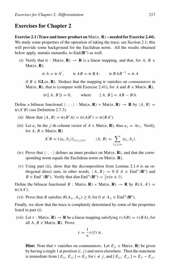
Exercises for Chapter 2: Differentiation 217
Exercises for Chapter 2
Exercise 2.1 (Trace and inner product on Mat(n,R) – needed for Exercise 2.44).We study some properties of the operation of taking the trace, see Section 2.1; thiswill provide some background for the Euclidean norm. All the results obtainedbelow apply, mutatis mutandis, to End(Rn) as well.
(i) Verify that tr : Mat(n,R) → R is a linear mapping, and that, for A, B ∈Mat(n,R),
tr A = tr At , tr AB = tr B A; tr B AB−1 = tr A
if B ∈ GL(n,R). Deduce that the mapping tr vanishes on commutators inMat(n,R), that is (compare with Exercise 2.41), for A and B ∈ Mat(n,R),
tr([ A, B ]) = 0, where [ A, B ] = AB − B A.
Define a bilinear functional 〈 · , · 〉 : Mat(n,R) × Mat(n,R) → R by 〈A, B〉 =tr(At B) (see Definition 2.7.3).
(ii) Show that 〈A, B〉 = tr(Bt A) = tr(ABt) = tr(B At).
(iii) Let a j be the j-th column vector of A ∈ Mat(n,R), thus a j = Ae j . Verify,for A, B ∈ Mat(n,R)
At B = (〈ai , b j 〉)1≤i, j≤n, 〈A, B〉 =∑
1≤ j≤n
〈a j , b j 〉.
(iv) Prove that 〈 · , · 〉 defines an inner product on Mat(n,R), and that the corre-sponding norm equals the Euclidean norm on Mat(n,R).
(v) Using part (ii), show that the decomposition from Lemma 2.1.4 is an or-thogonal direct sum, in other words, 〈 A, B 〉 = 0 if A ∈ End+(Rn) andB ∈ End−(Rn). Verify that dim End±(Rn) = 1
2 n(n ± 1).
Define the bilinear functional B : Mat(n,R) × Mat(n,R) → R by B(A, A′) =tr(AA′).
(vi) Prove that B satisfies B(A±, A±) ≷ 0, for 0 = A± ∈ End±(Rn).
Finally, we show that the trace is completely determined by some of the propertieslisted in part (i).
(vii) Let τ : Mat(n,R)→ R be a linear mapping satisfying τ(AB) = τ(B A), forall A, B ∈ Mat(n,R). Prove
τ = 1
nτ(I ) tr .
Hint: Note that τ vanishes on commutators. Let Ei j ∈ Mat(n,R) be givenby having a single 1 at position (i, j) and zeros elsewhere. Then the statementis immediate from [ Ei j , E j j ] = Ei j for i = j , and [ Ei j , E ji ] = Eii − E j j .
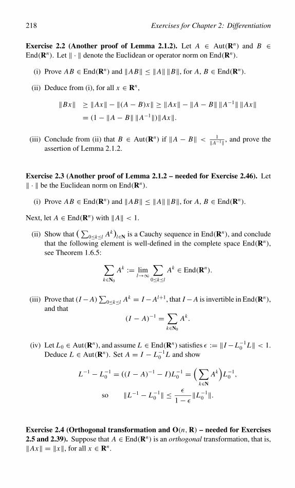
218 Exercises for Chapter 2: Differentiation
Exercise 2.2 (Another proof of Lemma 2.1.2). Let A ∈ Aut(Rn) and B ∈End(Rn). Let ‖ · ‖ denote the Euclidean or operator norm on End(Rn).
(i) Prove AB ∈ End(Rn) and ‖AB‖ ≤ ‖A‖ ‖B‖, for A, B ∈ End(Rn).
(ii) Deduce from (i), for all x ∈ Rn ,
‖Bx‖ ≥ ‖Ax‖ − ‖(A − B)x‖ ≥ ‖Ax‖ − ‖A − B‖ ‖A−1‖ ‖Ax‖= (1− ‖A − B‖ ‖A−1‖)‖Ax‖.
(iii) Conclude from (ii) that B ∈ Aut(Rn) if ‖A − B‖ < 1‖A−1‖ , and prove the
assertion of Lemma 2.1.2.
Exercise 2.3 (Another proof of Lemma 2.1.2 – needed for Exercise 2.46). Let‖ · ‖ be the Euclidean norm on End(Rn).
(i) Prove AB ∈ End(Rn) and ‖AB‖ ≤ ‖A‖ ‖B‖, for A, B ∈ End(Rn).
Next, let A ∈ End(Rn) with ‖A‖ < 1.
(ii) Show that (∑
0≤k≤l Ak)l∈N is a Cauchy sequence in End(Rn), and concludethat the following element is well-defined in the complete space End(Rn),see Theorem 1.6.5: ∑
k∈N0
Ak := liml→∞
∑0≤k≤l
Ak ∈ End(Rn).
(iii) Prove that (I−A)∑
0≤k≤l Ak = I−Al+1, that I−A is invertible in End(Rn),and that
(I − A)−1 =∑k∈N0
Ak .
(iv) Let L0 ∈ Aut(Rn), and assume L ∈ End(Rn) satisfies ε := ‖I−L−10 L‖ < 1.
Deduce L ∈ Aut(Rn). Set A = I − L−10 L and show
L−1 − L−10 = ((I − A)−1 − I )L−1
0 =(∑
k∈N
Ak)
L−10 ,
so ‖L−1 − L−10 ‖ ≤
ε
1− ε‖L−1
0 ‖.
Exercise 2.4 (Orthogonal transformation and O(n,R) – needed for Exercises2.5 and 2.39). Suppose that A ∈ End(Rn) is an orthogonal transformation, that is,‖Ax‖ = ‖x‖, for all x ∈ Rn .
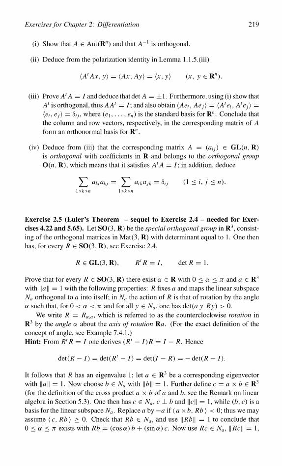
Exercises for Chapter 2: Differentiation 219
(i) Show that A ∈ Aut(Rn) and that A−1 is orthogonal.
(ii) Deduce from the polarization identity in Lemma 1.1.5.(iii)
〈At Ax, y〉 = 〈Ax, Ay〉 = 〈x, y〉 (x, y ∈ Rn).
(iii) Prove At A = I and deduce that det A = ±1. Furthermore, using (i) show thatAt is orthogonal, thus AAt = I ; and also obtain 〈Aei , Ae j 〉 = 〈At ei , At e j 〉 =〈ei , e j 〉 = δi j , where (e1, . . . , en) is the standard basis for Rn . Conclude thatthe column and row vectors, respectively, in the corresponding matrix of Aform an orthonormal basis for Rn .
(iv) Deduce from (iii) that the corresponding matrix A = (ai j ) ∈ GL(n,R)is orthogonal with coefficients in R and belongs to the orthogonal groupO(n,R), which means that it satisfies At A = I ; in addition, deduce∑
1≤k≤n
aki ak j =∑
1≤k≤n
aika jk = δi j (1 ≤ i, j ≤ n).
Exercise 2.5 (Euler’s Theorem – sequel to Exercise 2.4 – needed for Exer-cises 4.22 and 5.65). Let SO(3,R) be the special orthogonal group in R3, consist-ing of the orthogonal matrices in Mat(3,R) with determinant equal to 1. One thenhas, for every R ∈ SO(3,R), see Exercise 2.4,
R ∈ GL(3,R), Rt R = I, det R = 1.
Prove that for every R ∈ SO(3,R) there exist α ∈ R with 0 ≤ α ≤ π and a ∈ R3
with ‖a‖ = 1 with the following properties: R fixes a and maps the linear subspaceNa orthogonal to a into itself; in Na the action of R is that of rotation by the angleα such that, for 0 < α < π and for all y ∈ Na , one has det(a y Ry) > 0.
We write R = Rα,a , which is referred to as the counterclockwise rotation inR3 by the angle α about the axis of rotation Ra. (For the exact definition of theconcept of angle, see Example 7.4.1.)Hint: From Rt R = I one derives (Rt − I )R = I − R. Hence
det(R − I ) = det(Rt − I ) = det(I − R) = − det(R − I ).
It follows that R has an eigenvalue 1; let a ∈ R3 be a corresponding eigenvectorwith ‖a‖ = 1. Now choose b ∈ Na with ‖b‖ = 1. Further define c = a × b ∈ R3
(for the definition of the cross product a × b of a and b, see the Remark on linearalgebra in Section 5.3). One then has c ∈ Na , c ⊥ b and ‖c‖ = 1, while (b, c) is abasis for the linear subspace Na . Replace a by−a if 〈 a×b, Rb 〉 < 0; thus we mayassume 〈 c, Rb 〉 ≥ 0. Check that Rb ∈ Na , and use ‖Rb‖ = 1 to conclude that0 ≤ α ≤ π exists with Rb = (cosα) b + (sin α) c. Now use Rc ∈ Na , ‖Rc‖ = 1,
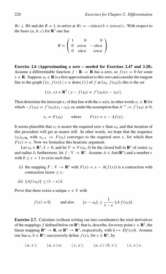
220 Exercises for Chapter 2: Differentiation
Rc ⊥ Rb and det R = 1, to arrive at Rc = −(sin α) b + (cosα) c. With respect tothe basis (a, b, c) for R3 one has
R = 1 0 0
0 cosα − sin α0 sin α cosα
.
Exercise 2.6 (Approximating a zero – needed for Exercises 2.47 and 3.28).Assume a differentiable function f : R → R has a zero, so f (x) = 0 for somex ∈ R. Suppose x0 ∈ R is a first approximation to this zero and consider the tangentline to the graph { (x, f (x)) | x ∈ dom( f ) } of f at (x0, f (x0)); this is the set
{ (x, y) ∈ R2 | y − f (x0) = f ′(x0)(x − x0) }.
Then determine the intercept x1 of that line with the x-axis, in other words x1 ∈ R forwhich− f (x0) = f ′(x0)(x1−x0), or, under the assumption that A−1 := f ′(x0) = 0,
x1 = F(x0) where F(x) = x − A f (x).
It seems plausible that x1 is nearer the required zero x than x0, and that iteration ofthis procedure will get us nearer still. In other words, we hope that the sequence(xk)k∈N0 with xk+1 := F(xk) converges to the required zero x , for which thenF(x) = x . Now we formalize this heuristic argument.
Let x0 ∈ Rn , δ > 0, and let V = V (x0; δ) be the closed ball in Rn of center x0
and radius δ; furthermore, let f : V → Rn . Assume A ∈ Aut(Rn) and a number εwith 0 ≤ ε < 1 to exist such that:
(i) the mapping F : V → Rn with F(x) = x − A( f (x)) is a contraction withcontraction factor ≤ ε;
(ii) ‖A f (x0)‖ ≤ (1− ε) δ.
Prove that there exists a unique x ∈ V with
f (x) = 0; and also ‖x − x0‖ ≤ 1
1− ε‖A f (x0)‖.
Exercise 2.7. Calculate (without writing out into coordinates) the total derivativesof the mappings f defined below on Rn; that is, describe, for every point x ∈ Rn , thelinear mapping Rn → R, or Rn → Rn , respectively, with h �→ D f (x)h. Assumeone has a, b ∈ Rn; successively define f (x), for x ∈ Rn , by
〈 a, x 〉; 〈 a, x 〉 a; 〈 x, x 〉; 〈 a, x 〉 〈 b, x 〉; 〈 x, x 〉 x .
Exercises for Chapter 2: Differentiation 221
Exercise 2.8. Let f : Rn → R be differentiable.
(i) Prove that f is constant if D f = 0.Hint: Recall that the result is known if n = 1, and use directional derivatives.
Let f : Rn → Rp be differentiable.
(ii) Prove that f is constant if D f = 0.
(iii) Let L ∈ Lin(Rn,Rp), and suppose D f (x) = L , for every x ∈ Rn . Prove theexistence of c ∈ Rp with f (x) = Lx + c, for every x ∈ Rn .
Exercise 2.9. Let f : Rn → R be homogeneous of degree 1, in the sense thatf (t x) = t f (x) for all x ∈ Rn and t ∈ R. Show that f has directional derivativesat 0 in all directions. Prove that f is differentiable at 0 if and only if f is linear,which is the case if and only if f is additive.
Exercise 2.10. Let g be as in Example 1.3.11. Then we define f : R2 → R by
f (x) = x2g(x) =
x1x32
x21 + x4
2
, x = 0;0, x = 0.
Show that Dv f (0) = 0, for all v ∈ R2; and deduce that D f (0) = 0, if f weredifferentiable at 0. Prove that Dv f (x) is well-defined, for all v and x ∈ R2, andthat v �→ Dv f (x) belongs to Lin(R2,R), for all x ∈ R2. Nevertheless, verify thatf is not differentiable at 0 by showing
limx2→0
| f (x22 , x2)|
‖(x22 , x2)‖ =
1
2.
Exercise 2.11. Define f : R2 → R by
f (x) =
x31
‖x‖2, x = 0;
0, x = 0.
Prove that f is continuous on R2. Show that directional derivatives of f at 0 in alldirections do exist. Verify, however, that f is not differentiable at 0. Compute
D1 f (x) = 1+ x22
x21 − x2
2
‖x‖4, D2 f (x) = −2x3
1 x2
‖x‖4(x ∈ R2 \ {0}).
In particular, both partial derivatives of f are well-defined on all of R2. Deducethat at least one of these partial derivatives has to be discontinuous at 0. To see thisexplicitly, note that
D1 f (t x) = D1 f (x), D2 f (t x) = D2 f (x) (t ∈ R \ {0}, x ∈ R2).
222 Exercises for Chapter 2: Differentiation
This means that the partial derivatives assume constant values along every linethrough the origin under omission of the origin. More precisely, in every neigh-borhood of 0 the function D1 f assumes every value in [ 0, 9
8 ] while D2 f assumesevery value in [− 3
8
√3, 3
8
√3 ]. Accordingly, in this case both partial derivatives are
discontinuous at 0.
Exercise 2.12 (Stronger version of Theorem 2.3.4). Let the notation be as inthat theorem, but with n ≥ 2. Show that the conclusion of the theorem remainsvalid under the weaker assumption that n − 1 partial derivatives of f exist in aneighborhood of a and are continuous at a while the remaining partial derivativemerely exists at a.Hint: Write
f (a + h)− f (a) =∑
n≥ j≥2
( f (a + h( j))− f (a + h( j−1)))+ f (a + h(1))− f (a).
Apply the method of the theorem to the sum over j and the definition of derivativeto the remaining difference.Background. As a consequence of this result we see that at least two differentpartial derivatives of f must be discontinuous at a if f fails to be differentiable ata, compare with Example 2.3.5.
Exercise 2.13. Let f j : R → R be differentiable, for 1 ≤ j ≤ n, and definef : Rn → R by f (x) = ∑
1≤ j≤n f j (x j ). Show that f is differentiable withderivative
D f (a) = ( f ′1(a1) · · · f ′n(an)) ∈ Lin(Rn,R) (a ∈ Rn).
Background. The fi might have discontinuous derivatives, which implies that thepartial derivatives of f are not necessarily continuous. Accordingly, continuity ofthe partial derivatives is not a necessary condition for the differentiability of f ,compare with Theorem 2.3.4.
Exercise 2.14. Show that the mappings ν1 and ν2 : Rn → R given by
ν1(x) =∑
1≤ j≤n
|x j |, ν2(x) = sup1≤ j≤n
|x j |,
respectively, are norms on Rn . Determine the set of points where νi is differentiable,for 1 ≤ i ≤ 2.
Exercise 2.15. Let f : Rn → R be a C1 function and k > 0, and assume that|D j f (x)| ≤ k, for 1 ≤ j ≤ n and x ∈ Rn .
Exercises for Chapter 2: Differentiation 223
(i) Prove that f is Lipschitz continuous with√
n k as a Lipschitz constant.
Next, let g : Rn \{0} → R be a C1 function and k > 0, and assume that |D j g(x)| ≤k, for 1 ≤ j ≤ n and x ∈ Rn \ {0}.
(ii) Show that if n ≥ 2, then g can be extended to a continuous function definedon all of Rn . Show that this is false if n = 1 by giving a counterexample.
Exercise 2.16. Define f : R2 → R by f (x) = log(1 + ‖x‖2). Compute thepartial derivatives D1 f , D2 f , and all second-order partial derivatives D2
1 f , D1 D2 f ,D2 D1 f and D2
2 f .
Exercise 2.17. Let g and h : R → R be twice differentiable functions. DefineU = { x ∈ R2 | x1 = 0 } and f : U → R by f (x) = x1g( x2
x1)+ h( x2
x1). Prove
x21 D2
1 f (x)+ 2x1x2 D1 D2 f (x)+ x22 D2
2 f (x) = 0 (x ∈ U ).
Exercise 2.18 (Independence of variable). Let U = R2 \ { (0, x2) | x2 ≥ 0 } anddefine f : U → R by
f (x) ={
x22 , x1 > 0 and x2 ≥ 0;
0, x1 < 0 or x2 < 0.
(i) Show that D1 f = 0 on all of U but that f is not independent of x1.
Now suppose that U ⊂ R2 is an open set having the property that for each x2 ∈ Rthe set { x1 ∈ R | (x1, x2) ∈ U } is an interval.
(ii) Prove that D1 f = 0 on all of U implies that f is independent of x1.
Exercise 2.19. Let h(t) = (cos t)sin t with dom(h) = { t ∈ R | cos t > 0 }. Proveh′(t) = (cos t)−1+sin t(cos2 t log cos t − sin2 t) in two different ways: by using thechain rule for R; and by writing
h = g ◦ f with f (t) = (cos t, sin t) and g(x) = x x21 .
Exercise 2.20. Define f : R2 → R2 and g : R2 → R2 by
f (x) = (x21 + x2
2 , sin x1x2), g(x) = (x1x2, ex2).
Then D(g ◦ f )(x) : R2 → R2 has the matrix(2x1 sin x1x2 + x2(x2
1 + x22) cos x1x2 2x2 sin x1x2 + x1(x2
1 + x22) cos x1x2
x2esin x1x2 cos x1x2 x1esin x1x2 cos x1x2
).
Prove this in two different ways: by using the chain rule; and by explicitly computingg ◦ f .
224 Exercises for Chapter 2: Differentiation
Exercise 2.21 (Eigenvalues and eigenvectors – needed for Exercise 3.41). LetA0 ∈ End(Rn) be fixed, and assume that x0 ∈ Rn and λ0 ∈ R satisfy
A0x0 = λ0x0, 〈x0, x0〉 = 1,
that is, x0 is a normalized eigenvector of A0 corresponding to the eigenvalue λ0.Define the mapping f : Rn × R → Rn × R by
f (x, λ) = (A0x − λx, 〈x, x〉 − 1 ).
The total derivative D f (x, λ) of f at (x, λ) belongs to End(Rn × R). Choose abasis (v1, . . . , vn) for Rn consisting of pairwise orthogonal vectors, with v1 = x0.The vectors (v1, 0), . . . , (vn, 0), (0, 1) then form a basis for Rn × R.
(i) Prove
D f (x, λ)(v j , 0) = ((A0 − λI )v j , 2〈 x, v j 〉) (1 ≤ j ≤ n),
D f (x, λ)(0, 1) = (−x, 0).
(ii) Show that the matrix of D f (x0, λ) with respect to the basis above, for allλ ∈ R, is of the following form:
λ0 − λ
0...
0
(A0 − λI )v2 · · · (A0 − λI )vn
−10...
02 0 · · · 0 0
.
(iii) Demonstrate by expansion according to the last column, and then accordingto the bottom row, that det D f (x0, λ) = 2 det B, with
A0 − λI =
λ0 − λ � · · · �
0...
0
B
.
Conclude that, for all λ = λ0, we have det D f (x0, λ) = 2det(A0 − λI )
λ0 − λ.
(iv) Prove
det D f (x0, λ0) = 2 limλ→λ0
det(A0 − λI )
λ0 − λ.
Exercises for Chapter 2: Differentiation 225
Exercise 2.22. Let U ⊂ Rn and V ⊂ Rp be open and let f : U → V be a C1
mapping. Define T f : U × Rn → Rp × Rp, the tangent mapping of f , to be themapping given by (see for more details Section 5.2)
T f (x, h) = ( f (x), D f (x)h).
Let V ⊂ Rp be open and let g : V → Rq be a C1 mapping. Show that the chainrule takes the natural form
T (g ◦ f ) = T g ◦ T f : U × Rn → Rq × Rq .
Exercise 2.23 (Another proof of Mean Value Theorem 2.5.3). Let the notation beas in that theorem. Let x ′ and x ∈ U be arbitrary and consider xt and xs ∈ L(x ′, x)as in Formula (2.15). Suppose m > k.
(i) By means of the definition of differentiability verify, for t > s and t − ssufficiently small,
‖ f (xt)− f (xs)− (t − s)D f (xs)(x − x ′)‖ ≤ (m − k)(t − s)‖x − x ′‖.Applying the reverse triangle inequality deduce
‖ f (xt)− f (xs)‖ ≤ m(t − s)‖x − x ′‖.
Set I = { t ∈ R | 0 ≤ t ≤ 1, ‖ f (xt)− f (x ′)‖ ≤ mt‖x − x ′‖ }.(ii) Use the continuity of f to obtain that I is closed. Note that 0 ∈ I and deduce
that I has a largest element 0 ≤ s ≤ 1.
(iii) Suppose that s < 1. Then prove by means of (i) and (ii), for s < t ≤ 1 witht − s sufficiently small,
‖ f (xt)− f (x ′)‖ ≤ ‖ f (xt)− f (xs)‖ + ‖ f (xs)− f (x ′)‖ ≤ mt‖x − x ′‖.Conclude that s = 1, and hence that ‖ f (x) − f (x ′)‖ ≤ m‖x − x ′‖. Nowuse the validity of this estimate for every m > k to obtain the Mean ValueTheorem.
Exercise 2.24 (Lipschitz continuity – needed for Exercise 3.26). Let U be aconvex open subset of Rn and let f : U → Rp be a differentiable mapping. Provethat the following assertions are equivalent.
(i) The mapping f is Lipschitz continuous on U with Lipschitz constant k.
(ii) ‖D f (x)‖ ≤ k, for all x ∈ U , where ‖ · ‖ denotes the operator norm.
226 Exercises for Chapter 2: Differentiation
Exercise 2.25. Let U ⊂ Rn be open and a ∈ U , and let f : U \ {a} → Rp bedifferentiable. Suppose there exists L ∈ Lin(Rn,Rp) with limx→a D f (x) = L .Prove that f is differentiable at a, with D f (a) = L .Hint: Apply the Mean Value Theorem to x �→ f (x)− Lx .
Exercise 2.26 (Criterion for injectivity). Let U ⊂ Rn be convex and open andlet f : U → Rn be differentiable. Assume that the self-adjoint part of D f (x) ispositive-definite for each x ∈ U , that is, 〈h, D f (x)h〉 > 0 if 0 = h ∈ Rn . Provethat f is injective.Hint: Suppose f (x) = f (x ′) where x ′ = x + h. Consider g : [ 0, 1 ] → R withg(t) = 〈h, f (x + th)〉. Note that g(0) = g(1) and deduce g′(τ ) = 0 for some0 < τ < 1.Background. For n = 1, this is the well-known result that a function f : I → Ron an interval I is strictly increasing and hence injective if f ′ > 0 on I .
Exercise 2.27 (Needed for Exercise 6.36). Let U ⊂ Rn be an open set and considera mapping f : U → Rp.
(i) Suppose f : U → Rp is differentiable on U and D f : U → Lin(Rn,Rp) iscontinuous at a. Using Example 2.5.4, deduce, for x and x ′ sufficiently closeto a,
f (x)− f (x ′) = D f (a)(x − x ′)+ ‖x − x ′‖ψ(x, x ′),
with lim(x,x ′)→(a,a) ψ(x, x ′) = 0.
(ii) Let f ∈ C1(U, Rp). Prove that for every compact K ⊂ U there existsa function λ : [ 0,∞ [ → [ 0,∞ [ with the following properties. First,limt↓0 λ(t) = 0; and further, for every x ∈ K and h ∈ Rn for which x+h ∈ K ,
‖ f (x + h)− f (x)− D f (x)(h)‖ ≤ ‖h‖ λ(‖h‖).
(iii) Let I be an open interval in R and let f ∈ C1(I,Rp). Define g : I× I → Rp
by
g(x, x ′) =
1
x − x ′( f (x)− f (x ′)), x = x ′;
D f (x), x = x ′.
Using part (i) prove that g is a C0 function on I × I and a C1 function onI × I \ ∪x∈I {(x, x)}.
(iv) In the notation of part (iii) suppose that D2 f (a) exists at a ∈ I . Prove thatg as in (iii) is differentiable at (a, a) with derivative Dg(a, a)(h1, h2) =
Exercises for Chapter 2: Differentiation 227
12 (h1 + h2)D2 f (a), for (h1, h2) ∈ R2.Hint: Consider h : I → Rp with
h(x) = f (x)− x D f (a)− 1
2(x − a)2 D2 f (a).
Verify, for x and x ′ ∈ I ,
1
x − x ′(h(x)− h(x ′)) = g(x, x ′)− g(a, a)− 1
2(x − a + x ′ − a)D2 f (a).
Next, show that for any ε > 0 there exists δ > 0 such that |h(x)− h(x ′)| <ε|x − x ′|(|x − a| + |x ′ − a|), for x and x ′ ∈ B(a; δ). To this end, apply thedefinition of the differentiability of D f at a to
Dh(x) = D f (x)− D f (a)− (x − a)D2 f (a).
Exercise 2.28. Let f : Rn → Rn be a differentiable mapping and assume that
sup{ ‖D f (x)‖Eucl | x ∈ Rn } ≤ ε < 1.
Prove that f is a contraction with contraction factor ≤ ε. Suppose F ⊂ Rn is aclosed subset satisfying f (F) ⊂ F . Show that f has a unique fixed point x ∈ F .
Exercise 2.29. Define f : R → R by f (x) = log(1+ ex). Show that | f ′(x)| < 1and that f has no fixed point in R.
Exercise 2.30. Let U = Rn \ {0}, and define f ∈ C∞(U ) by
f (x) =
log ‖x‖, if n = 2;
1
(2− n)
1
‖x‖n−2, if n = 2.
Prove grad f (x) = 1‖x‖n x , for n ∈ N and x ∈ U .
Exercise 2.31.
(i) For f1, f2 and f : Rn → R differentiable, prove grad( f1 f2) = f1 grad f2 +f2 grad f1, and grad 1
f = − 1f 2 grad f on Rn \ N (0).
(ii) Consider differentiable f : Rn → R and g : R → R. Verify grad(g ◦ f ) =(g′ ◦ f ) grad f .
(iii) Let f : Rn → Rp and g : Rp → R be differentiable. Show grad(g ◦ f ) =(D f )t(grad g)◦ f . Deduce for the j-th component function ( grad(g◦ f )) j =〈 (grad g) ◦ f, D j f 〉, where 1 ≤ j ≤ n.
228 Exercises for Chapter 2: Differentiation
Exercise 2.32 (Homogeneous function – needed for Exercises 2.40, 7.46, 7.62and 7.66). Let f : Rn \ {0} → R be a differentiable function.
(i) Let x ∈ Rn \ {0} be a fixed vector and define g : R+ → R by g(t) = f (t x).Show that g′(t) = D f (t x)(x).
Assume f to be positively homogeneous of degree d ∈ R, that is, f (t x) = td f (x),for all x = 0 and t ∈ R+.
(ii) Prove the following, known as Euler’s identity:
D f (x)(x) = 〈 x, grad f (x) 〉 = d f (x) (x ∈ Rn \ {0}).
(iii) Conversely, prove that f is positively homogeneous of degree d if we haveD f (x)(x) = d f (x), for every x ∈ Rn \ {0}.Hint: Calculate the derivative of t �→ t−d g(t), for t ∈ R+.
Exercise 2.33 (Analog of Rolle’s Theorem). Let U ⊂ Rn be an open set withcompact closure K . Suppose f : K → R is continuous on K , differentiable onU , and satisfies f (x) = 0, for all x ∈ K \ U . Show that there exists a ∈ U withgrad f (a) = 0.
Exercise 2.34. Consider f : R2 → R with f (x) = 4− (1− x1)2 − (1− x2)
2 onthe bounded set K ⊂ R2 bounded by the lines in R2 with the equations x1 = 0,x2 = 0, and x1 + x2 = 9, respectively. Prove that the absolute extrema of f on Dare: 4 assumed at (1, 1), and −61 at (9, 0) and (0, 9).Hint: The remaining candidates for extrema are: 3 at (1, 0) and (0, 1), 2 at 0, and− 41
2 at 12 (9, 9).
Exercise 2.35 (Linear regression). Consider the data points (x j , y j ) ∈ R2, for1 ≤ j ≤ n. The regression line for these data is the line in R2 that minimizes thesum of the squares of the vertical distances from the points to the line. Prove thatthe equation y = λx + c of this line is given by
λ = xy − x y
x2 − x2, c = y − λx = x2 y − x xy
x2 − x2.
Here we have used a bar to indicate the mean value of a variable in Rn , that is
x = 1
n
∑1≤ j≤n
x j , x2 = 1
n
∑1≤ j≤n
x2j , xy = 1
n
∑1≤ j≤n
x j y j , etc.
Exercises for Chapter 2: Differentiation 229
Exercise 2.36. Define f : R2 → R by f (x) = (x21 − x2)(3x2
1 − x2).
(i) Prove that f has 0 as a critical point, but not as a local extremum, by consid-ering f (0, t) and f (t, 2t2) for t near 0.
(ii) Show that the restriction of f to { x ∈ R2 | x2 = λx1 } attains a local minimum0 at 0, and a local minimum and maximum,− 1
12λ4(1± 2
3
√3), at 1
6λ(3±√
3),respectively.
Exercise 2.37 (Criterion for surjectivity – needed for Exercises 3.23 and 3.24).Let � : Rn → Rp be a differentiable mapping such that D�(x) ∈ Lin(Rn,Rp) issurjective, for all x ∈ Rn (thus n ≥ p). Let y ∈ Rp and define f : Rn → R bysetting f (x) = ‖�(x) − y‖. Furthermore, suppose that K ⊂ Rn is compact andthat there exists δ > 0 with
∃ x ∈ K with f (x) < δ, and f (x) ≥ δ (∀ x ∈ ∂K ).
Now prove that int(K ) = ∅ and that there is x ∈ int(K ) with �(x) = y.Hint: Note that the restriction to K of the square of f assumes its minimum inint(K ), and differentiate.
Exercise 2.38. Define f : R2 → R by
f (x) = x2
1 arctanx2
x1− x2
2 arctanx1
x2, x1x2 = 0;
0, x1x2 = 0.
Show D2 D1 f (0) = D1 D2 f (0).
Exercise 2.39 (Linear transformation and Laplacian – sequel to Exercise 2.4 –needed for Exercises 5.61, 7.61 and 8.32). Consider A ∈ End(Rn), with corre-sponding matrix (ai j )1≤i, j≤n ∈ Mat(n,R).
(i) Corroborate the known fact that D A(x) = A by proving D j Ai (x) = ai j , forall 1 ≤ i, j ≤ n and x ∈ Rn .
Next, assume that A ∈ Aut(n,R).
(ii) Verify that A : Rn → Rn is a bijective C∞ mapping, and that this is also trueof A−1.
Let g : Rn → R be a C2 function. The Laplace operator or Laplacian � assignsto g the C0 function
�g =∑
1≤k≤n
D2k g : Rn → R.
230 Exercises for Chapter 2: Differentiation
(iii) Prove that g ◦ A : Rn → R again is a C2 function.
(iv) Prove the following identities of C1 functions and of C0 functions, respec-tively, on Rn , for 1 ≤ k ≤ n:
Dk(g ◦ A) =∑
1≤ j≤n
a jk(D j g) ◦ A,
�(g ◦ A) =∑
1≤i, j≤n
( ∑1≤k≤n
aika jk
)(Di D j g) ◦ A.
(v) Using Exercise 2.4.(iv) prove the following invariance of the Laplacian underorthogonal transformations:
�(g ◦ A) = (�g) ◦ A ((A ∈ O(n,R)).
Exercise 2.40 (Sequel to Exercise 2.32). Let� be the Laplacian as in Exercise 2.39and let f and g : Rn → R be twice differentiable.
(i) Show �( f g) = f�g + 2〈grad f, grad g〉 + g� f .
Consider the norm ‖ · ‖ : Rn \ {0} → R and p ∈ R.
(ii) Prove that grad ‖ · ‖p(x) = p‖x‖p−2 x , for x ∈ Rn \ {0}, and furthermore,show �(‖ · ‖p) = p(p + n − 2)‖ · ‖p−2.
(iii) Demonstrate by means of part (i), for x ∈ Rn \ {0},�(‖ · ‖p f )(x) = ‖x‖p(� f )(x)+ 2p‖x‖p−2〈x, grad f (x)〉
+p(p + n − 2)‖x‖p−2 f (x).
Now suppose f to be positively homogeneous of degree d ∈ R, see Exercise 2.32.
(iv) On the strength of Euler’s identity verify that�(‖·‖2−n−2d f ) = ‖·‖2−n−2d� fon Rn \ {0}. In particular, �(‖ · ‖2−n) = 0 and �(‖ · ‖−n) = 2n‖ · ‖−n−2.
Exercise 2.41 (Angular momentum, Casimir and Euler operators – neededfor Exercises 3.9, 5.60 and 5.61). In quantum physics one defines the angularmomentum operator
L = (L1, L2, L3) : C∞(R3)→ C∞(R3, R3)
by (modulo a fourth root of unity), for f ∈ C∞(R3) and x ∈ R3,
(L f )(x) = ( grad f (x))× x ∈ R3.
(See the Remark on linear algebra in Section 5.3 for the definition of the crossproduct y × x of two vectors y and x in R3.)
Exercises for Chapter 2: Differentiation 231
(i) Verify (L1 f )(x) = x3 D2 f (x)− x2 D3 f (x).
The commutator [ A1, A2 ] of two linear operators A1 and A2 : C∞(R3)→ C∞(R3)
is defined by
[ A1, A2 ] = A1 A2 − A2 A1 : C∞(R3)→ C∞(R3).
(ii) Using Theorem 2.7.2 prove that the components of L satisfy the followingcommutator relations:
[ L j , L j+1 ] = L j+2 (1 ≤ j ≤ 3),
where the indices j are taken modulo 3.
Below, the elements of C∞(R3) will be taken to be complex-valued functions. Seti = √−1 and define H , X , Y : C∞(R3)→ C∞(R3) by
H = 2i L3, X = L1 + i L2, Y = −L1 + i L2.
(iii) Demonstrate that
1
iX = (x1 + i x2)D3 − x3(D1 + i D2) =: z
∂
∂x3− 2x3
∂
∂z,
1
iY = (x1 − i x2)D3 − x3(D1 − i D2) =: z
∂
∂x3− 2x3
∂
∂z,
where the notation is self-explanatory (see Lemma 8.3.10 as well as Exer-cise 8.17.(i)). Also prove
[ H, X ] = 2X, [ H, Y ] = −2Y, [ X, Y ] = H.
Background. These commutator relations are of great importance in thetheory of Lie algebras (see Definition 5.10.4 and Exercises 5.26.(iii) and5.59).
The Casimir operator C : C∞(R3)→ C∞(R3) is defined by C = −∑1≤ j≤3 L2
j .
(iv) Prove [C, L j ] = 0, for 1 ≤ j ≤ 3.
Denote by ‖ · ‖2 : C∞(R3) → C∞(R3) the multiplication operator satisfying(‖ · ‖2 f )(x) = ‖x‖2 f (x), and let E : C∞(R3)→ C∞(R3) be the Euler operatorgiven by (see Exercise 2.32.(ii))
(E f )(x) = 〈x, grad f (x)〉 =∑
1≤ j≤3
x j D j f (x).
232 Exercises for Chapter 2: Differentiation
(v) Prove −C + E(E + I ) = ‖ · ‖2�, where � denotes the Laplace operatorfrom Exercise 2.39.
(vi) Show using (iii)
C = 1
2(XY + Y X + 1
2H 2) = Y X + 1
2H + 1
4H 2.
Exercise 2.42 (Another proof of Proposition 2.7.6). The notation is as in thatproposition. Set xi = ai + hi ∈ Rn , for 1 ≤ i ≤ k. Then the k-linearity of T gives
T (x1, . . . , xk) = T (a1, . . . , ak)+∑
1≤i≤k
T (a1, . . . , ai−1, hi , xi+1, . . . , xk).
Each of the mappings (xi+1, . . . , xk) �→ T (a1, . . . , ai−1, hi , xi+1, . . . , xk) is (k−i)-linear. Deduce
T (a1, . . . , ai−1, hi , xi+1, . . . , xk) = T (a1, . . . , ai−1, hi , ai+1, . . . , ak)
+∑
1≤ j≤k−i
T (a1, . . . , ai−1, hi , ai+1, . . . , ai+ j−1, hi+ j , xi+ j+1, . . . , xk).
Now complete the proof of the proposition using Corollary 2.7.5.
Exercise 2.43 (Higher-order derivatives of bilinear mapping).
(i) Let A ∈ Lin(Rn,Rp). Prove that D2 A(a) = 0, for all a ∈ Rn .
(ii) Let T ∈ Lin2(Rn,Rp). Use Lemma 2.7.4 to show that D2T (a1, a2) ∈Lin2(Rn × Rn,Rp) and prove that it is given by, for ai , hi , ki ∈ Rn with1 ≤ i ≤ 2,
D2T (a1, a2)(h1, h2, k1, k2) = T (h1, k2)+ T (k1, h2).
Deduce D3T (a1, a2) = 0, for all (a1, a2) ∈ Rn × Rn .
Exercise 2.44 (Derivative of determinant – sequel to Exercise 2.1 – needed forExercises 2.51, 4.24 and 5.69). Let A ∈ Mat(n,R). We write A = (a1 · · · an),if a j ∈ Rn is the j-th column vector of A, for 1 ≤ j ≤ n. This means that weidentify Mat(n,R) with Rn × · · · × Rn (n copies). Furthermore, we denote by A
the complementary matrix as in Cramer’s rule (2.6).
(i) Consider the function det : Mat(n,R) → R as an element of Linn(Rn,R)via the identification above. Now prove that its derivative (D det)(A) ∈Lin(Mat(n,R),R) is given by
(D det)(A) = tr ◦A (A ∈ Mat(n,R)),
Exercises for Chapter 2: Differentiation 233
where tr denotes the trace of a matrix. More explicitly,
(D det)(A)H = tr(AH) = 〈 (A)t , H 〉 (H ∈ Mat(n,R)).
Here we use the result from Exercise 2.1.(ii). In particular, verify thatgrad(det)(A) = (A)t , the cofactor matrix, and
(�) (D det)(I ) = tr; (��) (D det)(A) = det A (tr ◦A−1),
for A ∈ GL(n,R), by means of Cramer’s rule.
(ii) Let X ∈ Mat(n,R) and define eX ∈ GL(n,R) as in Example 2.4.10. Show,for t ∈ R,
d
dtdet(et X ) = d
ds
∣∣∣∣s=0
det(e(s+t)X ) = d
ds
∣∣∣∣s=0
det(es X ) det(et X )
= tr X det(et X ).
Deduce by solving this differential equation that (compare also with For-mula (5.33))
det(et X ) = et tr X (t ∈ R, X ∈ Mat(n,R)).
(iii) Assume that A ∈ GL(n,R). Using det(A + H) = det A det(I + A−1 H),deduce (��) from (�) in (i). Now also derive (det A)A−1 = A from (i).
(iv) Assume that A : R → GL(n,R) is a differentiable mapping. Derive frompart (i) the following formula for the derivative of det ◦A : R → R:
1
det ◦A(det ◦A)′ = tr(A−1 ◦ D A),
in other words (compare with part (ii))
d
dt(log det A)(t) = tr
(A−1 d A
dt
)(t) (t ∈ R).
(v) Suppose that the mapping A : R → Mat(n,R) is differentiable and thatF : R → Mat(n,R) is continuous, while we have the differential equation
d A
dt(t) = F(t) A(t) (t ∈ R).
In this context, the Wronskianw ∈ C1(R) of A is defined asw(t) = det A(t).Use part (i), Exercise 2.1.(i) and Cramer’s rule to show, for t ∈ R,
dw
dt(t) = tr F(t) w(t), and deduce w(t) = w(0) e
∫ t0 tr F(τ ) dτ .
234 Exercises for Chapter 2: Differentiation
Exercise 2.45 (Derivatives of inverse acting in Aut(Rn) – needed for Exer-cises 2.46, 2.48, 2.49 and 2.51). We recall that Aut(Rn) is an open subset ofthe linear space End(Rn) and define the mapping F : Aut(Rn) → Aut(Rn) byF(A) = A−1. We want to prove that F is a C∞ mapping and to compute itsderivatives.
(i) Deduce from Formula (2.7) that F is differentiable. By differentiating theidentity AF(A) = I prove that DF(A), for A ∈ Aut(Rn), satisfies
DF(A) ∈ Lin ( End(Rn),End(Rn)) = End ( End(Rn)),
DF(A)H = −A−1 H A−1.
Generally speaking, we may not assume that A−1 and H commute, that is, A−1 H =H A−1. Next define
G : End(Rn)× End(Rn)→ End ( End(Rn)) by G(A, B)(H) = −AH B.
(ii) Prove that G is bilinear and, using Proposition 2.7.6, deduce that G is a C∞mapping.
Define � : End(Rn)→ End(Rn)× End(Rn) by �(B) = (B, B).
(iii) Verify that D�(B) = �, for all B ∈ End(Rn), and deduce that � is a C∞mapping.
(iv) Conclude from (i) that F satisfies the differential equation DF = G ◦� ◦ F .Using (ii), (iii) and mathematical induction conclude that F is a C∞ mapping.
(v) By means of the chain rule and (iv) show
D2 F(A) = DG(A−1, A−1)◦�◦G(A−1, A−1) ∈ Lin2 ( End(Rn),End(Rn)).
Now use Proposition 2.7.6 to obtain, for H1 and H2 ∈ End(Rn),
D2 F(A)(H1, H2) = (DG(A−1, A−1) ◦� ◦ G(A−1, A−1)H1)H2
= DG(A−1, A−1)(−A−1 H1 A−1,−A−1 H1 A−1)(H2)
= G(−A−1 H1 A−1, A−1)(H2)+ G(A−1,−A−1 H1 A−1)(H2)
= A−1 H1 A−1 H2 A−1 + A−1 H2 A−1 H1 A−1.
(vi) Using (i) and mathematical induction over k ∈ N show that Dk F(A) ∈Link ( End(Rn),End(Rn)) is given, for H1,…, Hk ∈ End(Rn), by
Dk F(A)(H1, . . . , Hk)
= (−1)k∑σ∈Sk
A−1 Hσ(1)A−1 Hσ(2)A
−1 · · · A−1 Hσ(k)A−1.
Exercises for Chapter 2: Differentiation 235
Verify that for n = 1 and A = t ∈ R we recover the known formula f (k)(t) =(−1)kk! t−(k+1) where f (t) = t−1.
Exercise 2.46 (Another proof for derivatives of inverse acting in Aut(Rn) –sequel to Exercises 2.3 and 2.45). Let the notation be as in the latter exercise. Inparticular, we have F : Aut(Rn)→ Aut(Rn)with F(A) = A−1. For K ∈ End(Rn)
with ‖K‖ < 1 deduce from Exercise 2.3.(iii)
F(I + K ) =∑
0≤ j≤k
(−K ) j + (−K )k+1 F(I + K ).
Furthermore, for A ∈ Aut(Rn) and H ∈ End(Rn), prove the equality F(A+ H) =F(I + A−1 H)F(A). Conclude, for ‖H‖ < ‖A−1‖−1,
(�)
F(A + H) =∑
0≤ j≤k
(−A−1 H) j A−1 + (−A−1 H)k+1 F(I + A−1 H)F(A)
=:∑
0≤ j≤k
(−1) j A−1 H A−1 · · · A−1 H A−1 + Rk(A, H).
Demonstrate‖Rk(A, H)‖ = O(‖H‖k+1), H → 0.
Using this and the fact that the sum in (�) is a polynomial of degree k in the variableH , conclude that (�) actually is the Taylor expansion of F at I . But this implies
Dk F(A)(H k) = (−1)kk! A−1 H A−1 · · · A−1 H A−1.
Now set, for H1, . . . , Hk ∈ End(Rn),
T (H1, . . . , Hk) = (−1)k∑σ∈Sk
A−1 Hσ(1)A−1 Hσ(2)A
−1 · · · A−1 Hσ(k)A−1.
Then T ∈ Link ( End(Rn),End(Rn)) is symmetric and T (H k) = Dk F(A)(H k).Since a generalization of the polarization identity from Lemma 1.1.5.(iii) impliesthat a symmetric k-linear mapping T is uniquely determined by H �→ T (H k), wesee that Dk F(A) = T .
Exercise 2.47 (Newton’s iteration method – sequel to Exercise 2.6 – needed forExercise 2.48). We come back to the approximation construction of Exercise 2.6,and we use its notation. In particular, V = V (x0; δ) and we now require f ∈C2(V,Rn). Near a zero of f to be determined, a much faster variant is Newton’siteration method, given by, for k ∈ N0,
(�) xk+1 = F(xk) where F(x) = x − D f (x)−1( f (x)).
This assumes that numbers c1 > 0 and c2 > 0 exist such that, with ‖ · ‖ equal tothe Euclidean or the operator norm,
D f (x) ∈ Aut(Rn), ‖D f (x)−1‖ ≤ c1, ‖D2 f (x)‖ ≤ c2 (x ∈ V ).
236 Exercises for Chapter 2: Differentiation
(i) Prove f (x) = f (x0)+ D f (x)(x − x0)− R1(x, x0− x) by Taylor expansionof f at x ; and based on the estimate for the remainder R1 from Theorem 2.8.3deduce that F : V → V , if in addition it is assumed
c1
(‖ f (x0)‖ + 1
2c2 δ
2)≤ δ.
This is the case if δ, and in its turn ‖ f (x0)‖, is sufficiently small. Deducethat (xk)k∈N0 is a sequence in V .
(ii) Apply f to (�) and use Taylor expansion of f of order 2 at xk to obtain
‖ f (xk+1)‖ ≤ 1
2c2 ‖D f (xk)
−1( f (xk))‖2 ≤ c3 ‖ f (xk)‖2,
with the notation c3 = 12 c2
1c2. Verify by mathematical induction over k ∈ N0
‖ f (xk)‖ ≤ 1
c3ε2k
if ε := c3 ‖ f (x0)‖.
If ε < 1 this proves that ( f (xk))k∈N0very rapidly converges to 0. In numerical
terms: the number of decimal zeros doubles with each iteration.
(iii) Deduce from part (ii), with d = c1c3= 2
c1c2,
‖xk+1 − xk‖ ≤ d ε2k(k ∈ N0),
from which one easily concludes that (xk)k∈N0 constitutes a Cauchy sequencein V . Prove that the limit x is the unique zero of f in V and that
‖xk − x‖ ≤ d∑l∈N0
ε2k+l ≤ d ε2k 1
1− ε(k ∈ N0).
Again, (xk) converges to the desired solution x at such a rate that each additionaliteration doubles the number of correct decimals. Newton’s iteration is the methodof choice when the calculation of D f (x)−1 (dependent on x) does not presenttoo much difficulty, see Example 1.7.3. The following figure gives a geometricalillustration of both the method of Exercise 2.6 and Newton’s iteration method.
Exercise 2.48 (Division by means of Newton’s iteration method – sequel toExercises 2.45 and 2.47). Given 0 = y ∈ R we want to approximate 1
y ∈ R by
means of Newton’s iteration method. To this end, consider f (x) = 1x − y and
choose a suitable initial value x0 for 1y .
(i) Show that the iteration takes the form
xk+1 = 2xk − yx2k (k ∈ N0).
Observe that this approximation to division requires only multiplication andaddition.
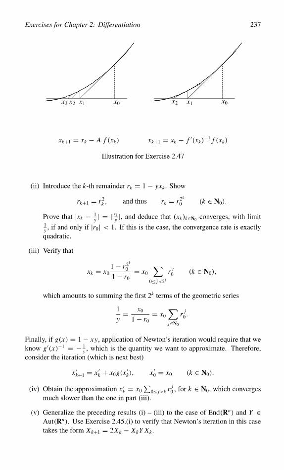
Exercises for Chapter 2: Differentiation 237
x0x1x2x0x1x2x3
xk+1 = xk − A f (xk) xk+1 = xk − f ′(xk)−1 f (xk)
Illustration for Exercise 2.47
(ii) Introduce the k-th remainder rk = 1− yxk . Show
rk+1 = r2k , and thus rk = r2k
0 (k ∈ N0).
Prove that |xk − 1y | = | rk
y |, and deduce that (xk)k∈N0 converges, with limit1y , if and only if |r0| < 1. If this is the case, the convergence rate is exactlyquadratic.
(iii) Verify that
xk = x01− r2k
0
1− r0= x0
∑0≤ j<2k
r j0 (k ∈ N0),
which amounts to summing the first 2k terms of the geometric series
1
y= x0
1− r0= x0
∑j∈N0
r j0 .
Finally, if g(x) = 1− xy, application of Newton’s iteration would require that weknow g′(x)−1 = − 1
y , which is the quantity we want to approximate. Therefore,consider the iteration (which is next best)
x ′k+1 = x ′k + x0g(x ′k), x ′0 = x0 (k ∈ N0).
(iv) Obtain the approximation x ′k = x0∑
0≤ j<k r j0 , for k ∈ N0, which converges
much slower than the one in part (iii).
(v) Generalize the preceding results (i) – (iii) to the case of End(Rn) and Y ∈Aut(Rn). Use Exercise 2.45.(i) to verify that Newton’s iteration in this casetakes the form Xk+1 = 2Xk − XkY Xk .
238 Exercises for Chapter 2: Differentiation
Exercise 2.49 (Sequel to Exercise 2.45). Suppose A : R → End+(Rn) is differ-entiable.
(i) Show that D A(t) ∈ Lin (R,End+(Rn)) � End+(Rn), for all t ∈ R.
Suppose that D A(t) is positive definite, for all t ∈ R.
(ii) Prove that A(t)− A(t ′) is positive definite, for all t > t ′ in R.
(iii) Now suppose that A(t) ∈ Aut(Rn), for all t ∈ R. By means of Exer-cise 2.45.(i) show that A(t)−1 − A(t ′)−1 is negative definite, for all t > t ′ inR.
Finally, assume that A0 and B0 ∈ End+(Rn) and that A0 − B0 is positive definite.Also assume A0 and B0 ∈ Aut(Rn).
(iv) Verify that A−10 −B−1
0 is negative definite by considering t �→ B0+t (A0−B0).
Exercise 2.50 (Action of Rn on C∞(Rn)). We recall the action of Rn on itself bytranslation, given by
Ta(x) = a + x (a, x ∈ Rn).
Obviously, TaTa′ = Ta+a′ . We now define an action of Rn on C∞(Rn) by assigningto a ∈ Rn and f ∈ C∞(Rn) the function Ta f ∈ C∞(Rn) given by
(Ta f )(x) = f (x − a) (x ∈ Rn).
Here we use the rule: “value of the transformed function at the transformed pointequals value of the original function at the original point”.
(i) Verify that we then have a group action, that is, for a and a′ ∈ Rn we have
(TaTa′) f = Ta(Ta′ f ) ( f ∈ C∞(Rn)).
For every a ∈ Rn we introduce ta by
ta : C∞(Rn)→ C∞(Rn) with ta f = d
dα
∣∣∣∣α=0
Tαa f.
(ii) Prove that ta f (x) = 〈 a, − grad f (x) 〉 (a ∈ Rn, f ∈ C∞(Rn)).Hint: For every x ∈ Rn we find
ta f (x) = d
dα
∣∣∣∣α=0
f (T−αa x) = D f (x)d
dα
∣∣∣∣α=0
(x − αa).
Exercises for Chapter 2: Differentiation 239
(iii) Demonstrate that from part (ii) follows, by means of Taylor expansion withrespect to the variable α ∈ R,
Tαa f = f + 〈αa, − grad f 〉 +O(α2), α→ 0 ( f ∈ C∞(Rn)).
Background. In view of this result, the operator − grad is also referred to as theinfinitesimal generator of the action of Rn on C∞(Rn).
Exercise 2.51 (Characteristic polynomial and Theorem of Hamilton–Cayley– sequel to Exercises 2.44 and 2.45). Denote the characteristic polynomial ofA ∈ End(Rn) by χA, that is
χA(λ) = det(λI − A) =:∑
0≤ j≤n
(−1) jσ j (A)λn− j .
Then σ0(A) = 1 and σn(A) = det A. In this exercise we derive a recursion formulafor the functions σ j : End(Rn)→ R by means of differential calculus.
(i) det A is a homogeneous function of degree n in the matrix coefficients of A.Using this fact, show by means of Taylor expansion of det : End(Rn)→ Rat I that
det(I + t A) =∑
0≤ j≤n
t j
j ! det ( j)(I )(A j ) (A ∈ End(Rn), t ∈ R).
Deduce
χA(λ) =∑
0≤ j≤n
(−1) j λn− j
j ! det ( j)(I )(A j ), σ j (A) = det ( j)(I )(A j )
j ! .
We define C : End(Rn)→ End(Rn) by C(A) = A, the complementary matrix ofA, and we recall the mapping F : Aut(Rn) → Aut(Rn) with F(A) = A−1 fromExercise 2.45. On Aut(Rn) Cramer’s rule from Formula (2.6) then can be writtenin the form C = det ·F .
(ii) Apply Leibniz’ rule, part (i) and Exercise 2.45.(vi) to this identity in order toget, for 0 ≤ k ≤ n and A ∈ Aut(Rn),
1
k!C(k)(I )(Ak) =
∑0≤ j≤k
det ( j)(I )(A j )
j !1
(k − j)!F(k− j)(I )(Ak− j )
=∑
0≤ j≤k
(−1)k− jσ j (A)Ak− j .
The coefficients of C(A) ∈ End(Rn) are homogeneous polynomials of degreen − 1 in those of A itself. Using this, deduce
C(A) = 1
(n − 1)!C(n−1)(I )(An−1) =
∑0≤ j<n
(−1)n−1− jσ j (A)An−1− j .
240 Exercises for Chapter 2: Differentiation
(iii) Next apply Cramer’s rule AC(A) = σn(A)I to obtain the following Theoremof Hamilton–Cayley, which asserts that A ∈ Aut(Rn) is annihilated by itsown characteristic polynomial χA,
0 = χA(A) =∑
0≤ j≤n
(−1) jσ j (A)An− j (A ∈ Aut(Rn)).
Using that Aut(Rn) is dense in End(Rn) show that the Theorem of Hamilton–Cayley is actually valid for all A ∈ End(Rn).
(iv) From Exercise 2.44.(i) we know that det (1) = tr ◦C . Differentiate this iden-tity k − 1 times at I and use Lemma 2.4.7 to obtain
det (k)(I )(Ak) = tr (C (k−1)(I )(Ak−1)A) (A ∈ End(Rn)).
Here we employed once more the density of Aut(Rn) in End(Rn) to derive theequality on End(Rn). By means of (i) and (ii) deduce the following recursionformula for the coefficients σk(A) of χA:
k σk(A) = (−1)k−1∑
0≤ j<k
(−1) jσ j (A) tr(Ak− j ) (A ∈ End(Rn)).
In particular,
χA(λ) = λn − tr(A)λn−1 + ( tr(A)2 − tr(A2))λn−2
2!−( tr(A)3 − 3 tr(A) tr(A2)+ 2 tr(A3))
λn−3
3! + · · · .
Exercise 2.52 (Newton’s Binomial Theorem, Leibniz’ rule and MultinomialTheorem – needed for Exercises 2.53, 2.55 and 7.22).
(i) Prove the following identities, for x and y ∈ Rn , a multi-index α ∈ Nn0, and
f and g ∈ C |α|(Rn), respectively
(x + y)α
α! =∑β≤α
xβ
β!yα−β
(α − β)! ,Dα( f g)
α! =∑β≤α
Dβ f
β!Dα−βg
(α − β)! .
Here the summation is over all multi-indices β ∈ Nn0 satisfying βi ≤ αi , for
every 1 ≤ i ≤ n.Hint: The former identity follows by Taylor’s formula applied to y �→ yα
α! ,while the latter is obtained by computation in two different ways of the co-efficient of the term of exponent α in the Taylor polynomial of order |α| off g.
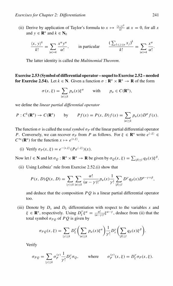
Exercises for Chapter 2: Differentiation 241
(ii) Derive by application of Taylor’s formula to x �→ 〈x,y〉kk! at x = 0, for all x
and y ∈ Rn and k ∈ N0
〈x, y〉kk! =
∑|α|=k
xα yα
α! , in particular(∑
1≤ j≤n x j )k
k! =∑|α|=k
xα
α! .
The latter identity is called the Multinomial Theorem.
Exercise 2.53 (Symbol of differential operator – sequel to Exercise 2.52 – neededfor Exercise 2.54). Let k ∈ N. Given a function σ : Rn × Rn → R of the form
σ(x, ξ) =∑|α|≤k
pα(x)ξα with pα ∈ C(Rn),
we define the linear partial differential operator
P : Ck(Rn)→ C(Rn) by P f (x) = P(x, D) f (x) =∑|α|≤k
pα(x)Dα f (x).
The function σ is called the total symbol σP of the linear partial differential operatorP . Conversely, we can recover σP from P as follows. For ξ ∈ Rn write e〈·,ξ〉 ∈C∞(Rn) for the function x �→ e〈x,ξ〉.
(i) Verify σP(x, ξ) = e−〈x,ξ〉(Pe〈·,ξ 〉)(x).
Now let l ∈ N and let σQ : Rn ×Rn → R be given by σQ(x, ξ) =∑|β|≤l qβ(x)ξβ .
(ii) Using Leibniz’ rule from Exercise 2.52.(i) show that
P(x, D)Q(x, D) =∑|γ |≤k
∑|α|≤k
α!(α − γ )! pα(x)
1
γ !∑|β|≤l
Dγ qβ(x)Dα−γ+β,
and deduce that the composition P Q is a linear partial differential operatortoo.
(iii) Denote by Dx and Dξ differentiation with respect to the variables x andξ ∈ Rn , respectively. Using Dγ
ξ ξα = α!
(α−γ )!ξα−γ , deduce from (ii) that the
total symbol σP Q of P Q is given by
σP Q(x, ξ) =∑|γ |≤k
Dγ
ξ
(∑|α|≤k
pα(x)ξα
)1
γ !Dγx
(∑|β|≤l
qβ(x)ξβ
).
Verify
σP Q =∑|γ |≤k
σ(γ )
P
1
γ !Dγx σQ, where σ
(γ )
P (x, ξ) = Dγ
ξ σP(x, ξ).
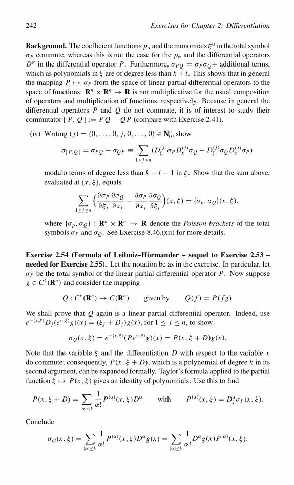
242 Exercises for Chapter 2: Differentiation
Background. The coefficient functions pα and the monomials ξα in the total symbolσP commute, whereas this is not the case for the pα and the differential operatorsDα in the differential operator P . Furthermore, σP Q = σPσQ+ additional terms,which as polynomials in ξ are of degree less than k + l. This shows that in generalthe mapping P �→ σP from the space of linear partial differential operators to thespace of functions: Rn × Rn → R is not multiplicative for the usual compositionof operators and multiplication of functions, respectively. Because in general thedifferential operators P and Q do not commute, it is of interest to study theircommutator [ P, Q ] := P Q − Q P (compare with Exercise 2.41).
(iv) Writing ( j) = (0, . . . , 0, j, 0, . . . , 0) ∈ Nn0, show
σ[ P,Q ] = σP Q − σQ P ≡∑
1≤ j≤n
(D( j)ξ σP D( j)
x σQ − D( j)ξ σQ D( j)
x σP)
modulo terms of degree less than k + l − 1 in ξ . Show that the sum above,evaluated at (x, ξ), equals∑
1≤ j≤n
(∂σP
∂ξ j
∂σQ
∂x j− ∂σP
∂x j
∂σQ
∂ξ j
)(x, ξ) = {σp, σQ}(x, ξ),
where {σp, σQ} : Rn × Rn → R denote the Poisson brackets of the totalsymbols σP and σQ . See Exercise 8.46.(xii) for more details.
Exercise 2.54 (Formula of Leibniz–Hörmander – sequel to Exercise 2.53 –needed for Exercise 2.55). Let the notation be as in the exercise. In particular, letσP be the total symbol of the linear partial differential operator P . Now supposeg ∈ Ck(Rn) and consider the mapping
Q : Ck(Rn)→ C(Rn) given by Q( f ) = P( f g).
We shall prove that Q again is a linear partial differential operator. Indeed, usee−〈x,ξ〉D j (e〈·,ξ〉g)(x) = (ξ j + D j )g(x), for 1 ≤ j ≤ n, to show
σQ(x, ξ) = e−〈x,ξ 〉(Pe〈·,ξ 〉g)(x) = P(x, ξ + D)g(x).
Note that the variable ξ and the differentiation D with respect to the variable xdo commute; consequently, P(x, ξ + D), which is a polynomial of degree k in itssecond argument, can be expanded formally. Taylor’s formula applied to the partialfunction ξ �→ P(x, ξ) gives an identity of polynomials. Use this to find
P(x, ξ + D) =∑|α|≤k
1
α! P(α)(x, ξ)Dα with P (α)(x, ξ) = Dα
ξ σP(x, ξ).
Conclude
σQ(x, ξ) =∑|α|≤k
1
α! P(α)(x, ξ)Dαg(x) =
∑|α|≤k
1
α!Dαg(x)P (α)(x, ξ).
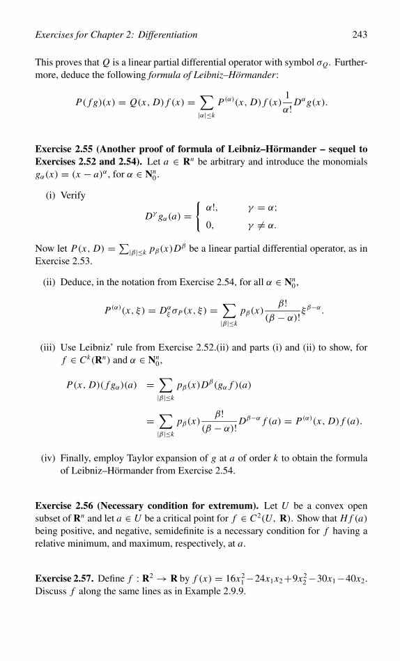
Exercises for Chapter 2: Differentiation 243
This proves that Q is a linear partial differential operator with symbol σQ . Further-more, deduce the following formula of Leibniz–Hörmander:
P( f g)(x) = Q(x, D) f (x) =∑|α|≤k
P (α)(x, D) f (x)1
α!Dαg(x).
Exercise 2.55 (Another proof of formula of Leibniz–Hörmander – sequel toExercises 2.52 and 2.54). Let a ∈ Rn be arbitrary and introduce the monomialsgα(x) = (x − a)α, for α ∈ Nn
0.
(i) Verify
Dγ gα(a) ={α!, γ = α;0, γ = α.
Now let P(x, D) =∑|β|≤k pβ(x)Dβ be a linear partial differential operator, as in
Exercise 2.53.
(ii) Deduce, in the notation from Exercise 2.54, for all α ∈ Nn0,
P (α)(x, ξ) = Dαξ σP(x, ξ) =
∑|β|≤k
pβ(x)β!
(β − α)!ξβ−α.
(iii) Use Leibniz’ rule from Exercise 2.52.(ii) and parts (i) and (ii) to show, forf ∈ Ck(Rn) and α ∈ Nn
0,
P(x, D)( f gα)(a) =∑|β|≤k
pβ(x)Dβ(gα f )(a)
=∑|β|≤k
pβ(x)β!
(β − α)!Dβ−α f (a) = P (α)(x, D) f (a).
(iv) Finally, employ Taylor expansion of g at a of order k to obtain the formulaof Leibniz–Hörmander from Exercise 2.54.
Exercise 2.56 (Necessary condition for extremum). Let U be a convex opensubset of Rn and let a ∈ U be a critical point for f ∈ C2(U, R). Show that H f (a)being positive, and negative, semidefinite is a necessary condition for f having arelative minimum, and maximum, respectively, at a.
Exercise 2.57. Define f : R2 → R by f (x) = 16x21−24x1x2+9x2
2−30x1−40x2.Discuss f along the same lines as in Example 2.9.9.
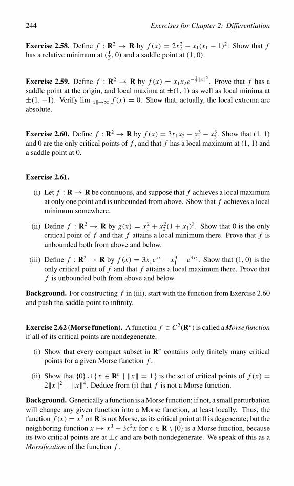
244 Exercises for Chapter 2: Differentiation
Exercise 2.58. Define f : R2 → R by f (x) = 2x22 − x1(x1 − 1)2. Show that f
has a relative minimum at ( 13 , 0) and a saddle point at (1, 0).
Exercise 2.59. Define f : R2 → R by f (x) = x1x2e−12 ‖x‖2
. Prove that f has asaddle point at the origin, and local maxima at ±(1, 1) as well as local minima at±(1,−1). Verify lim‖x‖→∞ f (x) = 0. Show that, actually, the local extrema areabsolute.
Exercise 2.60. Define f : R2 → R by f (x) = 3x1x2 − x31 − x3
2 . Show that (1, 1)and 0 are the only critical points of f , and that f has a local maximum at (1, 1) anda saddle point at 0.
Exercise 2.61.
(i) Let f : R → R be continuous, and suppose that f achieves a local maximumat only one point and is unbounded from above. Show that f achieves a localminimum somewhere.
(ii) Define f : R2 → R by g(x) = x21 + x2
2(1 + x1)3. Show that 0 is the only
critical point of f and that f attains a local minimum there. Prove that f isunbounded both from above and below.
(iii) Define f : R2 → R by f (x) = 3x1ex2 − x31 − e3x2 . Show that (1, 0) is the
only critical point of f and that f attains a local maximum there. Prove thatf is unbounded both from above and below.
Background. For constructing f in (iii), start with the function from Exercise 2.60and push the saddle point to infinity.
Exercise 2.62 (Morse function). A function f ∈ C2(Rn) is called a Morse functionif all of its critical points are nondegenerate.
(i) Show that every compact subset in Rn contains only finitely many criticalpoints for a given Morse function f .
(ii) Show that {0} ∪ { x ∈ Rn | ‖x‖ = 1 } is the set of critical points of f (x) =2‖x‖2 − ‖x‖4. Deduce from (i) that f is not a Morse function.
Background. Generically a function is a Morse function; if not, a small perturbationwill change any given function into a Morse function, at least locally. Thus, thefunction f (x) = x3 on R is not Morse, as its critical point at 0 is degenerate; but theneighboring function x �→ x3 − 3ε2x for ε ∈ R \ {0} is a Morse function, becauseits two critical points are at ±ε and are both nondegenerate. We speak of this as aMorsification of the function f .
Exercises for Chapter 2: Differentiation 245
Exercise 2.63 (Gram’s matrix and Cauchy–Schwarz inequality). Let v1, . . . , vd
be vectors in Rn and let G(v1, . . . , vd) ∈ Mat+(d,R) be Gram’s matrix associatedwith the vectors v1, . . . , vd as in Formula (2.4).
(i) Verify that G(v1, . . . , vd) is positive semidefinite and conclude that we havedet G(v1, . . . , vd) ≥ 0, which is known as the generalized Cauchy–Schwarzinequality.
(ii) Let d ≤ n. Prove that v1, . . . , vd are linearly dependent if and only ifdet G(v1, . . . , vd) = 0.
(iii) Apply (i) to vectors v1 and v2 in Rn . Note that one obtains the Cauchy–Schwarz inequality |〈v1, v2〉| ≤ ‖v1‖ ‖v2‖, which justifies the name given in(i).
(iv) Prove that for every triplet of vectors v1, v2 and v3 in Rn
( 〈v1, v2〉‖v1‖ ‖v2‖
)2
+( 〈v2, v3〉‖v2‖ ‖v3‖
)2
+( 〈v3, v1〉‖v3‖ ‖v1‖
)2
≤ 1+ 2〈v1, v2〉 〈v2, v3〉 〈v3, v1〉‖v1‖2 ‖v2‖2 ‖v3‖2
.
Exercise 2.64. Let A ∈ End+(Rn). Suppose that z = x+iy ∈ Cn is an eigenvectorcorresponding to the eigenvalue λ = µ + iν ∈ C, thus Az = λz. Show thatAx = µx − νy and Ay = νx + µy, and deduce
0 = 〈x, Ay〉 − 〈Ax, y〉 = ν(‖x‖2 + ‖y‖2).
Now verify the fact known from the Spectral Theorem 2.9.3 that the eigenvalues ofA are real, with corresponding eigenvectors in Rn .
Exercise 2.65 (Another proof of Spectral Theorem – sequel to Exercise 1.1).The following proof of Theorem 2.9.3 is not as efficient as the one in Section 2.9;on the other hand, it utilizes many techniques that have been studied in the currentchapter. The notation is as in the theorem and its proof; in particular, g : Rn → Ris given by g(x) = 〈Ax, x〉.
(i) Prove that there exists a ∈ Sn−1 such that g(x) ≤ g(a), for all x ∈ Sn−1.
Define L = Ra and recall from Exercise 1.1 the notation L⊥ for the orthocomple-ment of L .
(ii) Select h ∈ Sn−1 ∩ L⊥. Show that γh(t) = 1√1+t2
(a + th), for t ∈ R, defines
a mapping γh : R → Sn−1.
246 Exercises for Chapter 2: Differentiation
(iii) Deduce from (i) and (ii) that g ◦ γh : R → R has a critical point at 0, andconclude D(g ◦ γh)(0) = 0.
(iv) Prove Dγh(t) = (1+ t2)−32 (h− ta), for t ∈ R. Verify by means of the chain
rule that, for t ∈ R,
D(g ◦ γh)(t) = 2(1+ t2)−2((1− t2)〈Aa, h〉 + t (〈Ah, h〉 − 〈Aa, a〉)).
(v) Conclude from (iii) and (iv) that 〈Aa, h〉 = 0, for all h ∈ L⊥. Using Exer-cise 1.1.(iv) deduce that Aa ∈ (L⊥)⊥ = L = Ra, that is, there exists λ ∈ Rwith Aa = λa.
(vi) Show that A(L⊥) ⊂ L⊥ and that A acting as a linear operator in L⊥ isagain self-adjoint. Now deduce the assertion of the theorem by mathematicalinduction over n ∈ N.
Exercise 2.66 (Another proof of Lemma 2.1.1). Let A ∈ Lin(Rn,Rp). Use thenotation from Example 2.9.6 and Theorem 2.9.3; in particular, denote by λ1, . . . , λn
the eigenvalues of At A, each eigenvalue being repeated a number of times equal toits multiplicity.
(i) Show that λ j ≥ 0, for 1 ≤ j ≤ n.
(ii) Using (i) show, for h ∈ Rn \ {0},‖Ah‖2
‖h‖2= 〈A
t Ah, h〉‖h‖2
≤ max{ λ j | 1 ≤ j ≤ n } ≤∑
1≤ j≤n
λ j = tr(At A).
Conclude that the operator norm ‖ · ‖ satisfies
‖A‖2 = max{ λ j | 1 ≤ j ≤ n } and ‖A‖ ≤ ‖A‖Eucl ≤√
n ‖A‖.
(iii) Prove that ‖A‖ = 1 and ‖A‖Eucl =√
2, if
A =( cosα − sin α
sin α cosα
)(α ∈ R).
Exercise 2.67 (Minimax principle). Let the notation be as in the Spectral Theo-rem 2.9.3. In particular, suppose the eigenvalues of A to be enumerated in decreasingorder, each eigenvalue being repeated a number of times equal to its multiplicity;thus: λ1 ≥ λ2 ≥ · · · , with corresponding orthonormal eigenvectors a1, a2, . . . inRn .
Exercises for Chapter 2: Differentiation 247
(i) Let y ∈ Rn be arbitrary. Show that there exist α1 and α2 ∈ R with 〈α1a1 +α2a2, y〉 = 0 and
〈A(α1a1 + α2a2), α1a1 + α2a2〉 = λ1α21 + λ2α
22 ≥ λ2‖α1a1 + α2a2‖2.
Deduce, for the Rayleigh quotient R for A,
λ2 ≤ max{ R(x) | x ∈ Rn \ {0} with 〈x, y〉 = 0 }.On the other hand, by taking y = a1, verify that the maximum is preciselyλ2. Conclude that
λ2 = miny∈Rn
max{ R(x) | x ∈ Rn \ {0} with 〈x, y〉 = 0 }.
(ii) Now prove by mathematical induction over k ∈ N that λk+1 is given by
miny1,...,yk∈Rn
max{ R(x) | x ∈ Rn \ {0} with 〈x, y1〉 = · · · = 〈x, yk〉 = 0 }.
Background. This characterization of the eigenvalues by the minimax principle,and the algorithms based on it, do not require knowledge of the correspondingeigenvectors.
Exercise 2.68 (Polar decomposition of automorphism). Every A ∈ Aut(Rn) canbe represented in the form
A = K P, K ∈ O(Rn), P ∈ End+(Rn) ∩ Aut(Rn) positive definite,
and this decomposition is unique. We call P the polar or radial part of A. Provethis decomposition by noting that At A ∈ End+(Rn) is positive definite and has tobe equal to P K t K P = P2. Verify that there exists a basis (a1, . . . , an) for Rn suchthat At Aa j = λ2
j a j , where λ j > 0, for 1 ≤ j ≤ n. Next define P by Pa j = λ j a j ,for 1 ≤ j ≤ n. Then P is uniquely determined by At A and thus by A. Finally,define K = AP−1 and verify that K ∈ O(Rn).Background. Similarly one finds a decomposition A = P ′K ′, which generalizesthe polar decomposition x = r(cosα, sin α) of x ∈ R2 \ {0}. Note that O(Rn) isa subgroup of Aut(Rn), whereas the collection of self-adjoint P ∈ End+(Rn) ∩Aut(Rn) is not a subgroup (the product of two self-adjoint operators is self-adjointif and only if the operators commute). The polar decomposition is also known asthe Cartan decomposition.
Exercise 2.69. Define f : R+ × R → R by f (x, t) = 2x2t(x2+t2)2
. Show that∫ 10 f (x, t) dt = 1
1+x2 and deduce
limx→0
∫ 1
0f (x, t) dt =
∫ 1
0limx→0
f (x, t) dt.
Show that the conditions of the Continuity Theorem 2.10.2 are not satisfied.
248 Exercises for Chapter 2: Differentiation
Exercise 2.70 (Method of least squares). Let I = [ 0, 1 ]. Suppose we want toapproximate on I the continuous function f : I → R by an affine function of theform t �→ λt+c. The method of least squares would require that λ and c be chosento minimize the integral ∫ 1
0(λt + c − f (t))2 dt.
Show λ = 6∫ 1
0 (2t − 1) f (t) dt and c = 2∫ 1
0 (2− 3t) f (t) dt .
Exercise 2.71 (Sequel to Exercise 0.1). Prove
F(x) :=∫ π
2
0log(1+ x cos2 t) dt = π log
(1+√1+ x
2
)(x > −1).
Hint: Differentiate F , use the substitution t = arctan u from Exercise 0.1.(ii), and
deduce F ′(x) = π2
(1x − 1
x√
1+x
).
Exercise 2.72 (Sequel to Exercise 0.1).
(i) Prove∫ π
0 log(1− 2r cosα + r2) dα = 0, for |r | < 1.Hint: Differentiate with respect to r and use the substitution α = 2 arctan tfrom Exercise 0.1.(i).
(ii) Set e1 = (1, 0) and x(r, α) = r(cosα, sin α) ∈ R2. Deduce that we have∫ π
0 log ‖e1 − x(r, α)‖ dα = 0 for |r | < 1. Interpret this result geometrically.
(iii) The integral in (i) also can be computed along the lines of Exercise 0.18.(i). Infact, antidifferentiation of the geometric series (1− z)−1 =∑
k∈N0zk yields
the power series − log(1− z) =∑k∈N
zk
k which converges for z ∈ C, |z| ≤1, z = 1. Substitute z = reiα, use De Moivre’s formula, and take the realparts; this results in
log(1− 2r cosα + r2) = −2∑k∈N
rk
kcos kα.
Now interchange integration and summation.
(iv) Deduce from (i) that∫ π
0 log(1− 2r cosα + r2) dα = 2π log |r |, for |r | > 1.
Exercise 2.73 (∫
R e−x2dx = √π – needed for Exercise 2.87). Define f : R → R
by
f (a) =∫ 1
0
e−a2(1+t2)
1+ t2dt.
Exercises for Chapter 2: Differentiation 249
(i) Prove by a substitution of variables that f ′(a) = −2e−a2 ∫ a0 e−x2
dx , fora ∈ R.
Define g : R → R by g(a) = f (a)+(∫ a
0 e−x2dx
)2.
(ii) Prove that g′ = 0 on R; then conclude that g(a) = π4 , for all a ∈ R.
(iii) Prove that 0 ≤ f (a) ≤ e−a2, for all a ∈ R, and go on to show that (compare
with Example 6.10.8 and Exercises 6.41 and 6.50.(i))∫R
e−x2dx = √π.
Background. The motivation for the arguments above will become apparent inExercise 6.15.
Exercise 2.74 (Needed for Exercises 2.75 and 8.34). Let f : R2 → R be a C1
function that vanishes outside a bounded set in R2, and let h : R → R be a C1
function. Then
D( ∫ h(x)
−∞f (x, t) dt
)= f (x, h(x)) h′(x)+
∫ h(x)
−∞D1 f (x, t) dt (x ∈ R).
Hint: Define F : R2 → R by
F(y, z) =∫ z
−∞f (y, t) dt.
Verify that F is a function with continuous partial derivative D1 F : R2 → R givenby
D1 F(y, z) =∫ z
−∞D1 f (y, t) dt.
On account of the Fundamental Theorem of Integral Calculus on R, the functionD2 F exists and is continuous, because D2 F(y, z) = f (y, z). Conclude that Fis differentiable. Verify that the derivative of the mapping R → R with x �→F(x, h(x)) is given by
DF(x, h(x)) =(
D1 F(x, h(x)) D2 F(x, h(x)))(
1h′(x)
)
= D1 F(x, h(x))+ D2 F(x, h(x)) h′(x).
Combination of these arguments now yields the assertion.
250 Exercises for Chapter 2: Differentiation
Exercise 2.75 (Repeated antidifferentiation and Taylor’s formula – sequel toExercise 2.74 – needed for Exercises 6.105 and 6.108). Let f ∈ C(R) and k ∈ N.Define D0 f = f , and
D−k f (x) =∫ x
0
(x − t)k−1
(k − 1)! f (t) dt.
(i) Prove that (D−k f )′ = D−k+1 f by means of Exercise 2.74, and deduce fromthe Fundamental Theorem of Integral Calculus on R that
D−k f (x) =∫ x
0D−k+1 f (t) dt (k ∈ N).
Show (compare with Exercise 2.81)
(∗)∫ x
0
(x − t)k−1
(k − 1)! f (t) dt =∫ x
0
(∫ t1
0· · ·
(∫ tk−1
0f (tk) dtk
)· · · dt2
)dt1.
Background. The negative exponent in D−k f is explained by the fact thatit is a k-fold antiderivative of f . Furthermore, in this fashion the notation iscompatible with the one in Exercise 6.105.
In the light of the Fundamental Theorem of Integral Calculus on R the right–handside of (�) is seen to be a k-fold antiderivative, say g, of f . Evidently, therefore, ak-fold antiderivative can also be calculated by one integration.
(ii) Prove thatg( j)(0) = 0 (0 ≤ j < k).
Now assume f ∈ Ck+1(R) with k ∈ N0. Accordingly
h(x) :=∫ x
0
(x − t)k
k! f (k+1)(t) dt
is a (k + 1)-fold antiderivative of f (k+1), with h( j)(0) = 0, for 0 ≤ j ≤ k. On theother hand, f is also an (k + 1)-fold antiderivative of f (k+1).
(iii) Show, for x ∈ R,
f (x)−∑
0≤ j≤k
f ( j)(0)
j ! x j =∫ x
0
(x − t)k
k! f (k+1)(t) dt
= xk+1
k!∫ 1
0(1− t)k f (k+1)(t x) dt,
Taylor’s formula for f at 0, with the integral formula for the k-th remainder(see Lemma 2.8.2).
Exercises for Chapter 2: Differentiation 251
Exercise 2.76 (Higher-order generalization of Hadamard’s Lemma). Let U bea convex open subset of Rn and f ∈ C∞(U,Rp). Under these conditions a higher-order generalization of Hadamard’s Lemma 2.2.7 is as follows. For every k ∈ Nthere exists φk ∈ C∞(U,Link(Rn,Rp)) such that
(�) f (x) =∑
0≤ j<k
1
j !Dj f (a)((x − a) j )+ φk(x)((x − a)k),
(��) φk(a) = 1
k!Dk f (a).
We will prove this result in three steps.
(i) Let x and a ∈ U . Applying the Fundamental Theorem of Integral Calculuson R to the line segment L(a, x) ⊂ U and the mapping t �→ f (xt) withxt = a + t (x − a) (see Formula (2.15)) and using the continuity of D f ,deduce
f (x) = f (a)+∫ 1
0
d
dtf (xt) dt = f (a)+
∫ 1
0D f (xt) dt (x − a)
=: f (a)+ φ(x)(x − a).
Derive φ ∈ C∞(U,Lin(R,Rp)) on account of the differentiability of theintegral with respect to the parameter x ∈ U . Differentiate the identity abovewith respect to x at x = a to find φ(a) = D f (a).
Note that this proof of Hadamard’s Lemma is different from the one given inLemma 2.2.7.
(ii) Prove (�) by mathematical induction over k ∈ N. For k = 1 the result followsfrom part (i). Suppose the result has been obtained up to order k, and applypart (i) to φk ∈ C∞(U, Link(Rn,Rp)). On the strength of Lemma 2.7.4 weobtain φk+1 ∈ C∞(U, Link+1(Rn,Rp)) satisfying, for x near a,
φk(x) = φk(a)+ φk+1(x)(x − a) = 1
k!Dk f (a)+ φk+1(x)(x − a).
(iii) For verifying (��), replace k by k + 1 in (�) and differentiate the identitythus obtained k + 1 times with respect to x at x = a. We find Dk+1 f (a) =(k + 1)!φk+1(a).
(iv) In order to obtain an estimate for the remainder term, apply Corollary 2.7.5and verify
‖φk(x)((x − a)k)‖ = O(‖x − a‖k), x → a.
252 Exercises for Chapter 2: Differentiation
Background. It seems not to be possible to prove the higher-order generalizationof Hadamard’s Lemma without the integral representation used in part (i). Indeed,in (iii) we need the differentiability of φk+1(x) as such, without it being applied tothe (k + 1)-fold product of the vector x − a with itself.
Exercise 2.77. Calculate ∫ π2
− π2
∫ 2
1ex2 sin
( x1
x2
)dx2 dx1.
Exercise 2.78 (Interchanging order of integration implies integration by parts).Consider I = [ a, b ] and F ∈ C(I 2). Prove∫ b
a
∫ x
aF(x, y) dy dx =
∫ b
a
∫ b
yF(x, y) dx dy.
Let f and g ∈ C1(I ) and note f (x) = f (a) + ∫ xa f ′(y) dy and g(y) = g(b) +∫ y
a g′(x) dx , for x and y ∈ I . Now deduce∫ b
af (x)g′(x) dx = f (a)g(a)− f (b)g(b)−
∫ b
af ′(y)g(y) dy.
Exercise 2.79 (Sequel to Exercise 0.1 – needed for Exercise 6.50). Show bymeans of the substitution α = 2 arctan t from Exercise 0.1.(i) that∫ π
0
dα
1+ p cosα= π√
1− p2(|p| < 1).
Prove by changing the order of integration that∫ π
0
log(1+ x cosα)
cosαdα = π arcsin x (|x | < 1).
Exercise 2.80 (Sequel to Exercise 0.1). Let 0 < a < 1 and define f : [ 0, π2 ] ×[ 0, 1 ] → R by f (x, y) = 11−a2 y2 sin2 x
. Substitute x = arctan t in the first integral,as in Exercise 0.1.(ii), in order to show∫ π
2
0f (x, y) dx = π
2√
1− a2 y2,
∫ 1
0f (x, y) dy = 1
2a sin xlog
1+ a sin x
1− a sin x.
Deduce ∫ π2
0
1
sin xlog
1+ a sin x
1− a sin xdx = π arcsin a.
Exercises for Chapter 2: Differentiation 253
Exercise 2.81 (Exercise 2.75 revisited). Let f ∈ C(R). Prove, for all x ∈ R andk ∈ N (compare with Exercise 2.75)∫ x
0
(∫ t1
0· · ·
(∫ tk−1
0f (tk) dtk
)· · · dt2
)dt1 =
∫ x
0
(x − t)k−1
(k − 1)! f (t) dt.
Hint: If the choice is made to start from the left–hand side, use mathematicalinduction, and apply∫ x
0
(∫ t1
0· · · dt
)dt1 =
∫ x
0
(∫ x
t· · · dt1
)dt.
If the choice is to start from the right–hand side, use integration by parts.
Exercise 2.82. Using Example 2.10.14 and integration by parts show, for all x ∈ R,∫R+
1− cos xt
t2dt =
∫R+
sin2 xt
t2dt = π
2|x |.
Deduce, using sin2 2t = 4(sin2 t − sin4 t), and integration by parts, respectively,∫R+
sin4 t
t2dt = π
4,
∫R+
sin4 t
t4dt = π
3.
Exercise 2.83 (Sequel to Exercise 0.15). The notation is as in that exercise. Deducefrom part (iv) by means of differentiation that∫
R+
x p−1 log x
x + 1dx = −π
2 cos(πp)
sin2(πp)(0 < p < 1).
Exercise 2.84 (Sequel to Exercise 2.73 – needed for Exercise 6.83). Define F :R+ → R by
F(ξ) =∫
R+e−
12 x2
cos(ξ x) dx .
By differentiating F obtain F ′ + ξF = 0, and by using Exercise 2.73 deduceF(ξ) = √
π2 e−
12 ξ
2, for ξ ∈ R. Conclude that√π
2ξe−
12 ξ
2 =∫
R+xe−
12 x2
sin(ξ x) dx (ξ ∈ R).
254 Exercises for Chapter 2: Differentiation
Exercise 2.85 (Laplace’s integrals). Define F : R+ → R by
F(x) =∫
R+
sin xt
t (1+ t2)dt.
By differentiating F twice, obtain
F(x)− F ′′(x) =∫
R+
sin xt
tdt = π
2(x ∈ R+).
Since limx↓0 F(x) = 0 and F is bounded, deduce F(x) = π2 (1−e−x). Conclude, on
differentiation, that we have the following, known as Laplace’s integrals (comparewith Exercise 6.99.(iii))∫
R+
cos xt
1+ t2dt =
∫R+
t sin xt
1+ t2dt = π
2e−x (x ∈ R+).
Exercise 2.86. Prove for x ≥ 0∫R+
log(1+ x2t2)
1+ t2dt = π log(1+ x).
Hint: Use | 2xx2−1
( 11+t2 − 1
1+x2t2 )| ≤ 41+t2 , for all x ≥ √2.
Exercise 2.87 (Sequel to Exercise 2.73 – needed for Exercises 6.53, 6.97 and6.99).
(i) Using Exercise 2.73 prove for x ≥ 0
I (x) :=∫
R+e−t2− x2
t2 dt = 1
2
√π e−2x .
We now derive this result in another way.
(ii) Prove I (x) = √x∫
R+ e−x(t2+t−2) dt , for all x ∈ R+.
(iii) Write R+ as the union of ] 0, 1 ] and ] 1,∞ [. Replace t by t−1 on ] 0, 1 ] andconclude, for all x ∈ R+,
I (x) = √x∫ ∞
1(1+ t−2)e−x(t2+t−2) dt.
(iv) Prove by the substitution u = t − t−1 that I (x) = √x∫
R+ e−x(u2+2) du, forall x ∈ R+; and conclude that the identity in (i) holds.
Exercises for Chapter 2: Differentiation 255
(v) Let a and b ∈ R+. Prove∫R+
1√te−a2t− b2
t dt = √π e−2ab
a,
∫R+
1
t√
te−a2t− b2
t dt = √π e−2ab
b.
In particular, show
e−x = 1√π
∫R+
e−t
√t
e−x24t dt (x ≥ 0).
Exercise 2.88. For the verification of∫ 1
0
arctan t
t√
1− t2dt = π
2log(1+√2)
(note that the integrand is singular at t = 1) consider
F(x) =∫ 1
0
arctan xt
t√
1− t2dt (x ≥ 0).
Differentiation under the integral sign now yields
F ′(x) =∫ 1
0
1
1+ x2t2
1√1− t2
dt,
and with the substitution t = 1√1+u2
we compute the definite integral to be
F ′(x) =∫
R+
1
u2 + 1+ x2du = π
2
1√1+ x2
.
Integrating this identity we obtain a constant c ∈ R such that
F(x) = c + π
2arcsinh x = π
2log(x +
√1+ x2)+ c.
From F(0) = 0 we get c = 0, which implies the desired formula.
Exercise 2.89. Using interchange of integrations we can give another proof ofExercise 2.88. Verify
arctan t
t=
∫ 1
0
1
1+ t2 y2dy (t ∈ R).
With F as in Exercise 2.88, now deduce from the computations in that exercise,
F(1) =∫ 1
0
1√1− t2
∫ 1
0
1
1+ t2 y2dy dt =
∫ 1
0
∫ 1
0
1
(1+ t2 y2)√
1− t2dt dy
= π
2
∫ 1
0
1√1+ y2
dy = π
2log(1+√2).
256 Exercises for Chapter 2: Differentiation
Exercise 2.90 (Airy function – needed for Exercise 6.61). In the theory of lightan important role is played by the Airy function
Ai : R → C, Ai(x) = 1
2π
∫R
ei( 13 t3+xt) dt = 1
π
∫R+
cos(1
3t3 + xt) dt,
which satisfies Airy’s differential equation
u′′(x)− x u(x) = 0.
Although the integrand of Ai(x) does not die away as |t | → ∞, its increasinglyrapid oscillations induce convergence of the integral. However, the integral divergeswhen x lies in C \R. (The Airy function is defined as the inverse Fourier transformof the function t �→ ei 1
3 t3, see Theorem 6.11.6.)
Define
f± : C× R2 → C by f±(z, x, t) = e±i( 13 z3t3+zxt),
and consider, for z ∈ U± = { z ∈ C | 0 < ± arg z < π3 } and x ∈ R,
F±(z, x) = z∫
R+f±(z, x, t) dt.
(i) Verify 2π Ai(x) = F−(1, x)+F+(1, x). Further show limt→∞ f±(z, x, t) =0, for all (z, x) ∈ U± × R and that f±(z, x, t) remains bounded for t →∞,if (z, x) ∈ K±×R; here K± = U±, the closure of U±. In particular, 1 ∈ K±.
(ii) In order to prove convergence of the F±(z, x), show, for z ∈ C near 1,∫ ∞
1+|x |f±(z, x, t) dt =
[f±(z, x, t)
±i(z3t2 + zx)
]∞1+|x |
+∫ ∞
1+|x |2z3t
±i(z3t2 + zx)2f±(z, x, t) dt.
Using (i), prove that the boundary term converges and the integral convergesabsolutely and uniformly for z ∈ K± near 1 according to De la Vallée-Poussin’s test. Deduce that F±(z, x) is a continuous function of z ∈ K± near1.
(iii) Use z ∂ f±∂z (z, x, t) = t ∂ f±
∂t (z, x, t) to prove, for z ∈ U±,
∂F±∂z
(z, x) =∫
R+f±(z, x, t) dt +
∫R+
t∂ f±∂t
(z, x, t) dt
=∫
R+f±(z, x, t) dt + [
t f±(z, x, t)]∞
0 −∫
R+f±(z, x, t) dt = 0.
Conclude that F±(z, x) is a constant function of z ∈ U±. Using (ii) nowconclude that z �→ F±(z, x) actually is a constant function on K±. (Thismay also be proved on the basis of Cauchy’s Integral Theorem 8.3.11.)
Exercises for Chapter 2: Differentiation 257
(iv) Now, take z = z± := e±i π6 and deduce from (iii)
F±(1, x) = F±(z±, x) = z±∫
R+e−
13 t3±i z±xt dt
= e±i π6
∫R+
e−(13 t3+ 1
2 xt) e±12
√3 i xt dt.
Conclude that F±(1, ·) : R → C is a C∞ function and deduce that Ai : R →C is a C∞ function.
(v) Show, for x ∈ R,
∂2 F±∂x2
(z+, x)− x F±(z+, x) = ±i∫
R(−t2 ± i z±x) f±(z+, x, t) dt
= ±i∫
R+
∂ f±∂t
(z±, x, t) dt = ∓i.
Finally deduce that the Airy function satisfies Airy’s differential equation.
(vi) Deduce from (iv) that we have, with � denoting the Gamma function fromExercise 6.50 (see Exercise 6.61 for simplified expressions)
Ai(0) = 1
2π316
∫R+
e−uu−23 du = �( 1
3)
2π316
,
Ai′(0) = − 316
2π
∫R+
e−uu−13 du = −3
16�( 2
3)
2π.
(vii) Expand e±i z±xt in part (iv) in a power series to show
F±(1, x) = z±∑k∈N0
3k−2
3 �(k + 1
3
)(±i z±x)k
k! .
Using �(t +1) = t�(t) deduce the following power series expansion, whichconverges for all x ∈ R,
Ai(x) = Ai(0)(
1+ 1
3! x3 + 1 · 4
6! x6 + 1 · 4 · 79! x9 + · · ·
)+Ai′(0)
(x + 2
4! x4 + 2 · 5
7! x7 + 2 · 5 · 810! x10 + · · ·
).
Of course, this series also can be obtained by substitution of a power series∑k∈N0
ak xk in the differential equation and solving the recurrence relations.
(viii) Repeating the integration by parts in part (ii) prove Ai(x) = O(x−k), x →∞, for all k ∈ N.

Exercises for Chapter 3: Inverse Function Theorem 259
Exercises for Chapter 3
Exercise 3.1 (Needed for Exercise 6.59). Define � : R2+ → R2+ by
�(y) = (y1 + y2,y1
y2).
Prove that � is a C∞ diffeomorphism, with inverse � : R2+ → R2+ given by�(x) = x1
x2+1(x2, 1). Show that for �(y) = x
det D�(y) = − y1 + y2
y22
= −(x2 + 1)2
x1.
Exercise 3.2 (Needed for Exercises 3.19 and 6.64). Define � : R2 → R2 by
�(y) = y2(y1(1, 0)+ (1− y1)(0, 1)) = (y1 y2, (1− y1)y2).
(i) Prove that det D�(y) = y2, for y ∈ R2.
(ii) Prove that� : ] 0, 1 [ 2 → �2 is a C∞ diffeomorphism, if we define�2 ⊂ R2
as the triangular open set
�2 = { x ∈ R2+ | x1 + x2 < 1 }.
Exercise 3.3 (Needed for Exercise 3.22). Let� : R2 → R2 be defined by�(x) =(x1 + x2, x1 − x2).
(i) Prove that � is a C∞ diffeomorphism.
(ii) Determine �(U ) if U is the triangular open set given by
U = { (y1 y2, y1(1− y2)) ∈ R2 | (y1, y2) ∈ ] 0, 1 [× ] 0, 1 [ }.
Exercise 3.4. Let � : R2 → R2 be defined by �(x) = ex1(cos x2, sin x2).
(i) Determine im(�).
(ii) Prove that for every x ∈ R2 there exists a neighborhood U in R2 such that� : U → �(U ) is a C∞ diffeomorphism, but that � is not injective on allof R2.
(iii) Let x = (0, π3 ), y = �(x), and let� be the continuous inverse of�, defined
in a neighborhood of y, such that �(y) = x . Give an explicit formula for �.
260 Exercises for Chapter 3: Inverse Function Theorem
Exercise 3.5. Let U = ]−π, π [ × R+ ⊂ R2, and define � : U → R2 by
�(x) = (cos x1 cosh x2, sin x1 sinh x2).
(i) Prove that det D�(x) = −(sin2 x1 cosh2 x2 + cos2 x1 sinh2 x2) for x ∈ U ,and verify that � is regular on U .
(ii) Show that in general under � the lines x1 = a and x2 = b are mapped tohyperbolae and ellipses, respectively. Test whether � is injective.
(iii) Determine im(�).Hint: Assume y ∈ R2 \ { (y1, 0) | y1 ≤ 0 }. Then prove that
limx2→+∞
( y1
cosh x2
)2 +( y2
sinh x2
)2 = 0,
limx2↓0
( y1
cosh x2
)2 +( y2
sinh x2
)2 = ∞.
Conclude, by application of the Intermediate Value Theorem 1.9.5, that x2 ∈R+ exists such that, for some suitable x1 ∈ ]−π, π [ , one has
y1
cosh x2= cos x1,
y2
sinh x2= sin x1.
Exercise 3.6 (Cylindrical coordinates – needed for Exercise 3.8). Define � :R3 → R3 by
�(r, α, x3) = (r cosα, r sin α, x3).
(i) Prove that � is surjective, but not injective.
(ii) Find the points in R3 where � is regular.
(iii) Determine a maximal open set V in R3 such that � : V → �(V ) is a C∞diffeomorphism.
Background. The element (r, α, x3) ∈ V consists of the cylindrical coordinatesof x = �(r, α, x3).
Exercise 3.7 (Spherical coordinates – needed for Exercise 3.8). Define � :R3 → R3 by
�(r, α, θ) = r(cosα cos θ, sin α cos θ, sin θ).
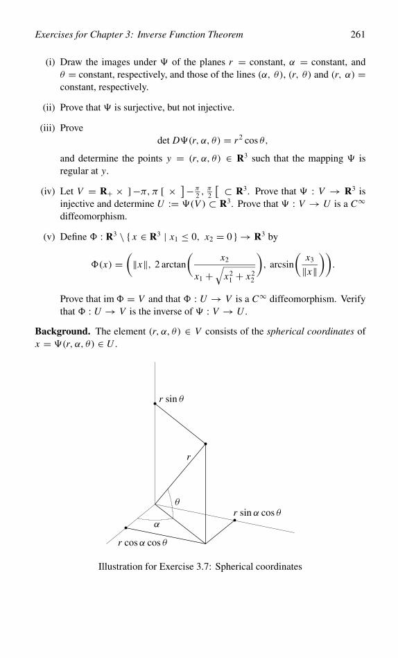
Exercises for Chapter 3: Inverse Function Theorem 261
(i) Draw the images under � of the planes r = constant, α = constant, andθ = constant, respectively, and those of the lines (α, θ), (r, θ) and (r, α) =constant, respectively.
(ii) Prove that � is surjective, but not injective.
(iii) Provedet D�(r, α, θ) = r2 cos θ,
and determine the points y = (r, α, θ) ∈ R3 such that the mapping � isregular at y.
(iv) Let V = R+ × ]−π, π [ × ]−π2 ,
π2
[ ⊂ R3. Prove that � : V → R3 isinjective and determine U := �(V ) ⊂ R3. Prove that � : V → U is a C∞diffeomorphism.
(v) Define � : R3 \ { x ∈ R3 | x1 ≤ 0, x2 = 0 } → R3 by
�(x) =(‖x‖, 2 arctan
(x2
x1 +√
x21 + x2
2
), arcsin
(x3
‖x‖))
.
Prove that im� = V and that � : U → V is a C∞ diffeomorphism. Verifythat � : U → V is the inverse of � : V → U .
Background. The element (r, α, θ) ∈ V consists of the spherical coordinates ofx = �(r, α, θ) ∈ U .
α
r cosα cos θ
r sin α cos θ
r sin θ
r
θ
Illustration for Exercise 3.7: Spherical coordinates
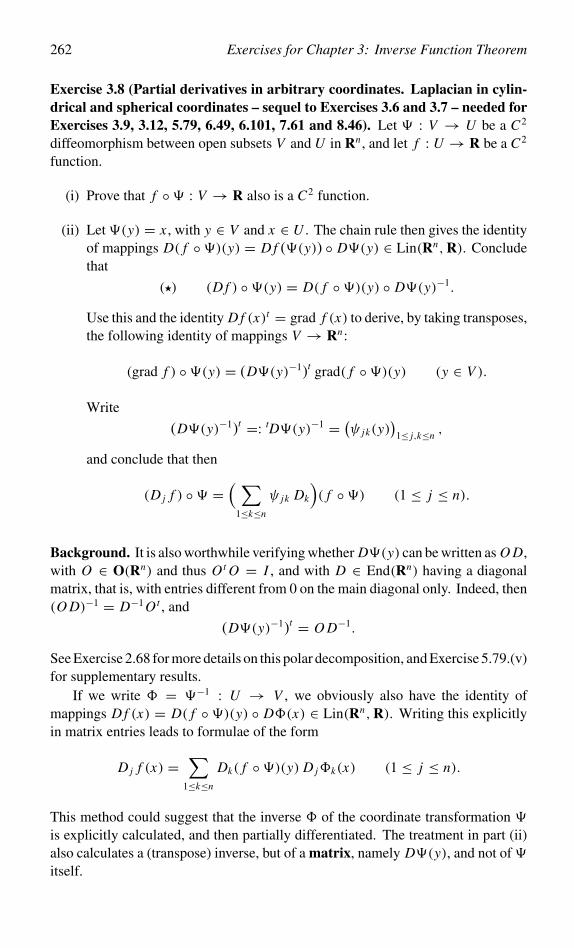
262 Exercises for Chapter 3: Inverse Function Theorem
Exercise 3.8 (Partial derivatives in arbitrary coordinates. Laplacian in cylin-drical and spherical coordinates – sequel to Exercises 3.6 and 3.7 – needed forExercises 3.9, 3.12, 5.79, 6.49, 6.101, 7.61 and 8.46). Let � : V → U be a C2
diffeomorphism between open subsets V and U in Rn , and let f : U → R be a C2
function.
(i) Prove that f ◦� : V → R also is a C2 function.
(ii) Let �(y) = x , with y ∈ V and x ∈ U . The chain rule then gives the identityof mappings D( f ◦�)(y) = D f (�(y)) ◦ D�(y) ∈ Lin(Rn,R). Concludethat
(�) (D f ) ◦�(y) = D( f ◦�)(y) ◦ D�(y)−1.
Use this and the identity D f (x)t = grad f (x) to derive, by taking transposes,the following identity of mappings V → Rn:
(grad f ) ◦�(y) = (D�(y)−1)t grad( f ◦�)(y) (y ∈ V ).
Write
(D�(y)−1)t =: tD�(y)−1 = (ψ jk(y)
)1≤ j,k≤n
,
and conclude that then
(D j f ) ◦� =( ∑
1≤k≤n
ψ jk Dk
)( f ◦�) (1 ≤ j ≤ n).
Background. It is also worthwhile verifying whether D�(y) can be written as O D,with O ∈ O(Rn) and thus Ot O = I , and with D ∈ End(Rn) having a diagonalmatrix, that is, with entries different from 0 on the main diagonal only. Indeed, then(O D)−1 = D−1 Ot , and
(D�(y)−1)t = O D−1.
See Exercise 2.68 for more details on this polar decomposition, and Exercise 5.79.(v)for supplementary results.
If we write � = �−1 : U → V , we obviously also have the identity ofmappings D f (x) = D( f ◦ �)(y) ◦ D�(x) ∈ Lin(Rn,R). Writing this explicitlyin matrix entries leads to formulae of the form
D j f (x) =∑
1≤k≤n
Dk( f ◦�)(y) D j�k(x) (1 ≤ j ≤ n).
This method could suggest that the inverse � of the coordinate transformation �is explicitly calculated, and then partially differentiated. The treatment in part (ii)also calculates a (transpose) inverse, but of a matrix, namely D�(y), and not of �itself.
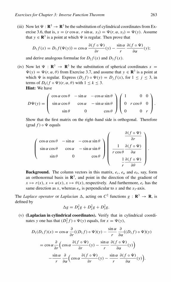
Exercises for Chapter 3: Inverse Function Theorem 263
(iii) Now let� : R3 → R3 be the substitution of cylindrical coordinates from Ex-ercise 3.6, that is, x = (r cosα, r sin α, x3) = �(r, α, x3) = �(y). Assumethat y ∈ R3 is a point at which � is regular. Then prove that
D1 f (x) = D1 f (�(y)) = cosα∂( f ◦�)
∂r(y)− sin α
r
∂( f ◦�)∂α
(y);and derive analogous formulae for D2 f (x) and D3 f (x).
(iv) Now let � : R3 → R3 be the substitution of spherical coordinates x =�(y) = �(r, α, θ) from Exercise 3.7, and assume that y ∈ R3 is a point atwhich � is regular. Express (D j f ) ◦ �(y) = D j f (x), for 1 ≤ j ≤ 3, interms of Dk( f ◦�)(r, α, θ) with 1 ≤ k ≤ 3.Hint: We have
D�(y) =
cosα cos θ − sin α − cosα sin θ
sin α cos θ cosα − sin α sin θ
sin θ 0 cos θ
1 0 0
0 r cos θ 0
0 0 r
.
Show that the first matrix on the right–hand side is orthogonal. Therefore(grad f ) ◦� equals
cosα cos θ − sin α − cosα sin θ
sin α cos θ cosα − sin α sin θ
sin θ 0 cos θ
∂( f ◦�)∂r
1
r cos θ
∂( f ◦�)∂α
1
r
∂( f ◦�)∂θ
.
Background. The column vectors in this matrix, er , eα and eθ , say, forman orthonormal basis in R3, and point in the direction of the gradient ofx �→ r(x), x �→ α(x), x �→ θ(x), respectively. And furthermore, er has thesame direction as x , whereas eα is perpendicular to x and the x3-axis.
The Laplace operator or Laplacian �, acting on C2 functions g : R3 → R, isdefined by
�g = D21 g + D2
2 g + D23 g.
(v) (Laplacian in cylindrical coordinates). Verify that in cylindrical coordi-nates y one has that (D2
1 f ) ◦�(y) equals, for x = �(y),
D1(D1 f )(x) = cosα∂
∂r((D1 f ) ◦�)(y)− sin α
r
∂
∂α((D1 f ) ◦�)(y)
= cosα∂
∂r
(cosα
∂( f ◦�)∂r
(y)− sin α
r
∂( f ◦�)∂α
(y))
−sin α
r
∂
∂α
(cosα
∂( f ◦�)∂r
(y)− sin α
r
∂( f ◦�)∂α
(y)).

264 Exercises for Chapter 3: Inverse Function Theorem
Now prove
(� f ) ◦� =(
1
r2
((r∂
∂r
)2 + ∂2
∂α2
)+ ∂2
∂x23
)( f ◦�).
(vi) (Laplacian in spherical coordinates). Verify that this is given by the for-mula
(� f ) ◦� = 1
r2
(∂
∂r
(r2 ∂
∂r
)+ 1
cos2 θ
(∂2
∂α2+
(cos θ
∂
∂θ
)2))
( f ◦�).
Background. In the Exercises 3.16, 7.60 and 7.61 we will encounter formulae for� on U in arbitrary coordinates in V . Our proofs in the last two cases require thetheory of integration.
Exercise 3.9 (Angular momentum, Casimir, and Euler operators in sphericalcoordinates – sequel to Exercises 2.41 and 3.8 – needed for Exercises 3.17, 5.60and 6.68). We employ the notations from the Exercises 2.41 and 3.8.
(i) Prove by means of Exercise 3.8.(iv) that for the substitution x = �(r, α, θ) ∈R3 of spherical coordinates one has
(L1 f ) ◦� =(
cosα tan θ∂
∂α− sin α
∂
∂θ
)( f ◦�),
(L2 f ) ◦� =(
sin α tan θ∂
∂α+ cosα
∂
∂θ
)( f ◦�),
(L3 f ) ◦� = − ∂
∂α( f ◦�),
where L is the angular momentum operator.
(ii) Show that the following assertions concerning f ∈ C∞(R3) are equivalent.First, the equation L f = 0 is satisfied. And second, f ◦� is independent ofα and θ , that is, f is a function of the distance to the origin.
(iii) Conclude that (see Exercise 2.41 for the definitions of H , X and Y )
(H f ) ◦� = −2i∂
∂α( f ◦�) =: H ∗( f ◦�),
(X f ) ◦� = eiα(
tan θ∂
∂α+ i
∂
∂θ
)( f ◦�) =: X∗( f ◦�),
(Y f ) ◦� = −e−iα(
tan θ∂
∂α− i
∂
∂θ
)( f ◦�) = =: Y ∗( f ◦�).
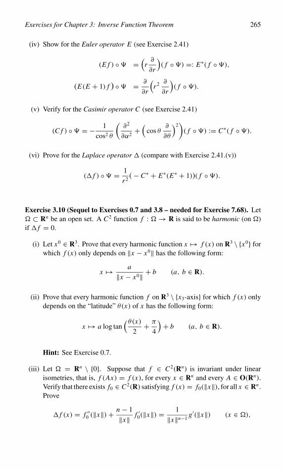
Exercises for Chapter 3: Inverse Function Theorem 265
(iv) Show for the Euler operator E (see Exercise 2.41)
(E f ) ◦� =(
r∂
∂r
)( f ◦�) =: E∗( f ◦�),
(E(E + 1) f ) ◦� = ∂
∂r
(r2 ∂
∂r
)( f ◦�).
(v) Verify for the Casimir operator C (see Exercise 2.41)
(C f ) ◦� = − 1
cos2 θ
(∂2
∂α2+
(cos θ
∂
∂θ
)2)( f ◦�) := C∗( f ◦�).
(vi) Prove for the Laplace operator � (compare with Exercise 2.41.(v))
(� f ) ◦� = 1
r2(− C∗ + E∗(E∗ + 1))( f ◦�).
Exercise 3.10 (Sequel to Exercises 0.7 and 3.8 – needed for Exercise 7.68). Let� ⊂ Rn be an open set. A C2 function f : �→ R is said to be harmonic (on �)if � f = 0.
(i) Let x0 ∈ R3. Prove that every harmonic function x �→ f (x) on R3 \ {x0} forwhich f (x) only depends on ‖x − x0‖ has the following form:
x �→ a
‖x − x0‖ + b (a, b ∈ R).
(ii) Prove that every harmonic function f on R3 \ {x3-axis} for which f (x) onlydepends on the “latitude” θ(x) of x has the following form:
x �→ a log tan(θ(x)
2+ π
4
)+ b (a, b ∈ R).
Hint: See Exercise 0.7.
(iii) Let � = Rn \ {0}. Suppose that f ∈ C2(Rn) is invariant under linearisometries, that is, f (Ax) = f (x), for every x ∈ Rn and every A ∈ O(Rn).Verify that there exists f0 ∈ C2(R) satisfying f (x) = f0(‖x‖), for all x ∈ Rn .Prove
� f (x) = f ′′0 (‖x‖)+ n − 1
‖x‖ f ′0(‖x‖) = 1
‖x‖n−1g′(‖x‖) (x ∈ �),
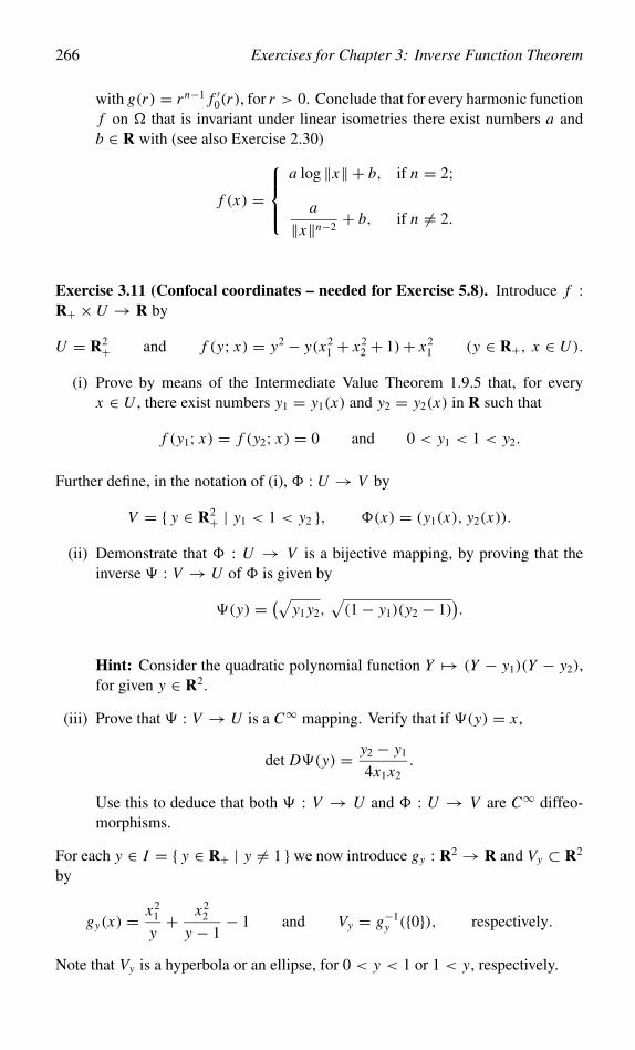
266 Exercises for Chapter 3: Inverse Function Theorem
with g(r) = rn−1 f ′0(r), for r > 0. Conclude that for every harmonic functionf on � that is invariant under linear isometries there exist numbers a andb ∈ R with (see also Exercise 2.30)
f (x) =
a log ‖x‖ + b, if n = 2;
a
‖x‖n−2+ b, if n = 2.
Exercise 3.11 (Confocal coordinates – needed for Exercise 5.8). Introduce f :R+ ×U → R by
U = R2+ and f (y; x) = y2 − y(x2
1 + x22 + 1)+ x2
1 (y ∈ R+, x ∈ U ).
(i) Prove by means of the Intermediate Value Theorem 1.9.5 that, for everyx ∈ U , there exist numbers y1 = y1(x) and y2 = y2(x) in R such that
f (y1; x) = f (y2; x) = 0 and 0 < y1 < 1 < y2.
Further define, in the notation of (i), � : U → V by
V = { y ∈ R2+ | y1 < 1 < y2 }, �(x) = (y1(x), y2(x)).
(ii) Demonstrate that � : U → V is a bijective mapping, by proving that theinverse � : V → U of � is given by
�(y) = (√y1 y2,
√(1− y1)(y2 − 1)
).
Hint: Consider the quadratic polynomial function Y �→ (Y − y1)(Y − y2),for given y ∈ R2.
(iii) Prove that � : V → U is a C∞ mapping. Verify that if �(y) = x ,
det D�(y) = y2 − y1
4x1x2.
Use this to deduce that both � : V → U and � : U → V are C∞ diffeo-morphisms.
For each y ∈ I = { y ∈ R+ | y = 1 } we now introduce gy : R2 → R and Vy ⊂ R2
by
gy(x) = x21
y+ x2
2
y − 1− 1 and Vy = g−1
y ({0}), respectively.
Note that Vy is a hyperbola or an ellipse, for 0 < y < 1 or 1 < y, respectively.
Exercises for Chapter 3: Inverse Function Theorem 267
(iv) Show x ∈ Vy if and only if f (y; x) = 0.
(v) Prove by means of (ii) that every x ∈ U lies on precisely one hyperbolaand also on precisely one ellipse from the collection { Vy | y ∈ I }. Andconversely, that for every y ∈ V the hyperbola Vy1 and the ellipse Vy2 haveprecisely one point of intersection, namely x = �(y), in U .
Background. The last property in (v) is remarkable, and is related to the fact thatall conics Vy possess the same foci, namely at the points (±1, 0). The elementy = (y1(x), y2(x)) ∈ V consists of the confocal coordinates of the point x ∈ U .
Exercise 3.12 (Moving frame, and gradient in arbitrary coordinates – sequel toExercise 3.8 – needed for Exercises 3.16 and 7.60). Let � : V → U be a C2 dif-feomorphism between open subsets V and U in Rn . Then (D1�(y), . . . , Dn�(y))is a basis for Rn for every y ∈ V ; the mapping
y �→ (D1�(y), . . . , Dn�(y)) : V → (Rn)n
is called the moving frame on V determined by �. Define the C1 mapping G :V → GL(n,R) by
G(y) = D�(y)t ◦ D�(y) = ( 〈 D j�(y), Dk�(y) 〉 )1≤ j,k≤n =: (g jk(y))1≤ j,k≤n.
In other words, G(y) is Gram’s matrix associated with the set of basis vectorsD1�(y), . . . , Dn�(y) in Rn . Write the inverse matrix of G(y) as
G(y)−1 = (g jk(y))1≤ j,k≤n (y ∈ V ).
(i) Prove that det G(y) = ( det D�(y))2, for all y ∈ V .
Therefore we can introduce the C1 function
√g : V → R by
√g(y) = √
det G(y) = | det D�(y)|.Furthermore, let f ∈ C1(U ) and consider grad f : U → Rn . We now wish toexpress the mapping (grad f ) ◦� : V → Rn in terms of derivatives of f ◦� andof the moving frame on V determined by �.
(ii) Using Exercise 3.8.(ii), demonstrate the following equality of vectors in Rn:
(grad f ) ◦�(y) = D�(y)G(y)−1 grad( f ◦�)(y) (y ∈ V ).
(iii) Verify the following equality on V of Rn-valued mappings:
(grad f ) ◦� =∑
1≤ j,k≤n
g jk Dk( f ◦�) D j�.
268 Exercises for Chapter 3: Inverse Function Theorem
Exercise 3.13 (Divergence of vector field – needed for Exercise 3.14). Let Ube an open subset of Rn and suppose f : U → Rn to be a C1 mapping; in thisexercise we refer to f as a vector field. We define the divergence of the vector fieldf , notation: div f , as the function Rn → R with (see Definition 7.8.3 for moredetails)
div f (x) = tr D f (x) =∑
1≤i≤n
Di fi (x).
As usual, tr denotes the trace of an element in End(Rn). Next, let h ∈ C1(U ).Using (h f )i = h fi for 1 ≤ i ≤ n, show, for x ∈ U ,
div(h f )(x) = Dh(x) f (x)+ h(x) div f (x) = (h div f )(x)+ 〈grad h, f 〉(x).
Exercise 3.14 (Divergence in arbitrary coordinates – sequel to Exercises 2.1,2.44, 3.12 and 3.13 – needed for Exercises 3.15, 3.16, 7.60, 8.40 and 8.41). LetU and V be open subsets of Rn , and let � : V → U be a C2 diffeomorphism.Next, assume f : U → Rn to be a C1 mapping; in this exercise we refer to f asa vector field. Then we define the C1 vector field �∗ f , the pullback of f under �(see Exercise 3.15), by
�∗ f : V → Rn with �∗ f (y) = D�(y)−1( f ◦�)(y) (y ∈ V ).
Denote the component functions of �∗ f by f (i) ∈ C1(V,R), for 1 ≤ i ≤ n; thus,if (e1, . . . , en) is the standard basis for Rn ,
�∗ f =∑
1≤i≤n
f (i)ei .
(i) Verify the identity of vectors in Rn:
f ◦�(y) =∑
1≤i≤n
f (i)(y) Di�(y) (y ∈ V ).
In other words, the f (i) are the component functions of f ◦ � : V → Rn
with respect to the moving frame on V determined by � in the terminologyof Exercise 3.12.
The formula for (div f ) ◦ � : V → R, the divergence of f on U in the newcoordinates in V , in terms of the pullback of f under � or, what amounts to thesame, the component functions of f with respect to the moving frame determinedby �, now reads, with
√g as in Exercise 3.12,
(div f ) ◦� = 1√g
div(√
g�∗ f ) = 1√g
∑1≤i≤n
Di (√
g f (i)) : V → R.
We derive this identity in the following three steps; see Exercises 7.60 and 8.40 forother proofs.
Exercises for Chapter 3: Inverse Function Theorem 269
(ii) Differentiate the equality f ◦� = D� ·�∗ f : V → Rn to obtain, for y ∈ Vand h ∈ Rn ,
D f (�(y)) D�(y)h = D2�(y)(h, �∗ f (y))+ D�(y) D(�∗ f )(y)h
= D2�(y)(�∗ f (y), h)+ D�(y) D(�∗ f )(y)h,
according to Theorem 2.7.9. Deduce the following identity of transformationsin End(Rn):
(D f ) ◦�(y) = D2�(y)(�∗ f (y)) D�(y)−1
+D�(y) D(�∗ f )(y) D�(y)−1.
By taking traces and using Exercise 2.1.(i) verify, for y ∈ V ,
(div f ) ◦�(y) = div(�∗ f )(y)+ tr (D�(y)−1 D2�(y)�∗ f (y)).
(iii) Show by means of the chain rule and (��) in Exercise 2.44.(i), for y ∈ V andh ∈ Rn ,
D(det D�)(y)h = (D det)(D�(y)) D2�(y)h
= det D�(y) tr (D�(y)−1 D2�(y)h).
Conclude, for y ∈ V , that
tr (D�(y)−1 D2�(y)�∗ f (y)) = 1
det D�(y)D(det D�)(y)�∗ f (y)
= 1√g(y)
D(√
g)(y)�∗ f (y).
(iv) Use parts (ii) and (iii) and Exercise 3.13 to prove, for y ∈ V ,
(div f ) ◦�(y) = div(�∗ f )(y)+ 1√g(y)
D(√
g)(y)�∗ f (y)
=( 1√
gdiv(
√g�∗ f )
)(y).
Exercise 3.15 (Pullback and pushforward of vector field under diffeomorphism– sequel to Exercise 3.14 – needed for Exercise 8.46). (Compare with Exer-cise 5.79.) Pullback of objects (functions, vector fields, etc.) is associated withsubstitution of variables in these objects. Indeed, let U be an open subset of Rn andconsider a vector field f : U → Rn and the corresponding ordinary differentialequation dx
dt (t) = f (x(t)) for a C1 mapping x : R → U . Let V be an open set inRn and let � : V → U be a C1 diffeomorphism.
270 Exercises for Chapter 3: Inverse Function Theorem
(i) Prove that the substitution of variables x = �(y) leads to the followingequation, where �∗ f is as in Exercise 3.14:
D�(y(t))dy
dt(t) = f ◦�(y(t)), thus
dy
dt(t) = �∗ f (y(t)).
(ii) Verify that the formula for the divergence in Exercise 3.14 may be written as
�∗ ◦ div = 1√g
div (√
g ·�∗).
Now let � : U → V be a C1 diffeomorphism. For every vector field f : U → Rn
we define the vector field�∗ f , the pushforward of f under�, by�∗ f = (�−1)∗ f .
(iii) Prove that �∗ f : V → Rn with
�∗ f (y) = D�(�−1(y))( f ◦�−1)(y) = (D� · f ) ◦�−1(y).
Exercise 3.16 (Laplacian in arbitrary coordinates – sequel to Exercises 3.12and 3.14 – needed for Exercise 7.61). Let U be an open subset of Rn and supposef : U → R to be a C2 function. We define the Laplace operator, or Laplacian,acting on f via
� f = div(grad f ) =∑
1≤ j≤n
D2j f : U → R.
Now suppose that V is an open subset of Rn and that � : V → U is a C2
diffeomorphism. Then we have the following equality of mappings V → R for �on U in the new coordinates in V :
(� f ) ◦� = 1√g
div (√
g G−1 grad( f ◦�))
= 1√g
∑1≤i, j≤n
Di (√
g gi j D j )( f ◦�)
=( ∑
1≤i, j≤n
gi j Di D j +∑
1≤ j≤n
(1√g
∑1≤i≤n
Di (√
g gi j ))
D j
)( f ◦�).
We derive this identity in the following two steps, see Exercise 7.61 for anotherproof.
(i) Using Exercise 3.12.(ii) prove that the pullback of the vector field grad f :U → Rn under � is given by
�∗(grad f ) : V → Rn, �∗(grad f )(y) = G(y)−1 grad( f ◦�)(y).
Exercises for Chapter 3: Inverse Function Theorem 271
(ii) Next apply Exercise 3.14.(iv) to obtain
(� f ) ◦� = div(grad f ) ◦� = 1√g
div (√
gG−1 grad( f ◦�)).
Phrased differently, �∗ ◦� = 1√g div (
√g · G−1 · grad ◦�∗).
The diffeomorphism � is said to be orthogonal if G(y) is a diagonal matrix, for ally ∈ V .
(iii) Verify that for an orthogonal � the formula for (� f ) ◦� takes the followingform:
(�) (� f ) ◦� = 1√g
∑1≤ j≤n
D j
(∏i = j ‖Di�‖‖D j�‖ D j
)( f ◦�).
(iv) Verify that the condition of orthogonality of� does not imply that D�(y), fory ∈ V , is an orthogonal matrix. Prove that the formula in Exercise 2.39.(v) isa special case of (�). Show that the transition to polar coordinates in R2, or tospherical coordinates in R3, respectively, is an orthogonal diffeomorphism.Also calculate� in polar and spherical coordinates, respectively, making useof (�); compare with Exercise 3.8.(v) and (vi). See also Exercise 5.13.
Background. Note that D�(y) enters the formula for (� f ) ◦ �(y) only throughits polar part, in the terminology of Exercise 2.68.
Exercise 3.17 (Casimir operator and spherical functions – sequel to Exer-cises 0.4 and 3.9 – needed for Exercises 5.61 and 6.68). We use the notationsfrom Exercises 0.4 and 3.9. Let l ∈ N0 and m ∈ Z with |m| ≤ l. Define thespherical function
Y ml : V := ]−π, π [×
]−π
2,π
2
[→ C by Y m
l (α, θ) = eimαP |m|l (sin θ).
Let Yl be the (2l + 1)-dimensional linear space over C of functions spanned by theY m
l , for |m| ≤ l. Through the linear isomorphism
ι : f �→ ι f with f (α, θ) = (ι f )(cosα cos θ, sin α cos θ, sin θ),
continuous functions f on V are identified with continuous functions ι f on the unitsphere S2 in R3. In particular, ιY 0
l is a function on S2 invariant under rotationsabout the x3-axis. The zeros of ιY 0
l divide S2 up into parallel zones, and for thatreason Y 0
l is called a zonal spherical function.
272 Exercises for Chapter 3: Inverse Function Theorem
(i) Prove by means of Exercise 0.4.(iii) that the differential operator C∗ fromExercise 3.9.(v) acts on Yl as the linear operator of multiplication by thescalar l(l + 1), that is, as a linear operator with a single eigenvalue, namelyl(l + 1), with multiplicity 2l + 1. To do so, verify that
C∗ Y ml = l(l + 1) Y m
l (|m| ≤ l).
(ii) Prove by means of Exercises 3.9.(iii) and 0.4.(iv) that Yl is invariant underthe action of the differential operators H ∗, X∗ and Y ∗. To do so, defineY l+1
l = Y−l−1l = 0, and prove by means of Exercise 0.4.(iv), for all |m| ≤ l,
H ∗ Y ml = 2m Y m
l , X∗ Y ml = i Y m+1
l ,
Y ∗ Y ml = −i (l + m)(l − m + 1)Y m−1
l .
Another description of this result is as follows. Define Vj = 1j !(Y
∗) j Y ll ∈ Yl , for
0 ≤ j ≤ 2l.
(iii) Show that
Vj = (−i) j (2l)!(2l − j)! Y l− j
l (0 ≤ j ≤ 2l).
Then prove, for 0 ≤ j ≤ 2l,
(�)H ∗ Vj = (2l − 2 j) Vj , X∗ Vj = (2l + 1− j) Vj−1,
Y ∗ Vj = ( j + 1)Vj+1.
See Exercise 5.62.(v) for the matrices of X∗ and Y ∗ with respect to the basis(V0, . . . , V2l), if l in that exercise is replaced by 2l.
(iv) Conclude by means of Exercise 3.9.(vi) that the functions
�(r, α, θ) �→ rl Y ml (α, θ) and �(r, α, θ) �→ r−l−1 Y m
l (α, θ)
are harmonic (see Exercise 3.10) on the dense open subset im(�) ⊂ R3. Forthis reason the functions ιY m
l are also called spherical harmonic functions,for they are restrictions to the two-sphere of harmonic functions on R3.
Background. In quantum physics this is the theory of the (orbital) angular mo-mentum operator associated with a particle without spin in a rotationally symmetricforce field (see also Exercise 5.61). Here l is called the orbital angular momentumquantum number and m the magnetic quantum number. The fact that the space Yl
of spherical functions is (2l+ 1)-dimensional constitutes the mathematical basis ofthe (elementary) theory of the Zeeman effect: the splitting of an atomic spectral lineinto an odd number of lines upon application of an external magnetic field alongthe x3-axis.
Exercises for Chapter 3: Inverse Function Theorem 273
Exercise 3.18 (Spherical coordinates in Rn – needed for Exercises 5.13 and7.21). If x in Rn satisfies x2
1 + · · · + x2n = r2 with r ≥ 0, then there exists a unique
element θn−2 ∈ [−π2 ,
π2 ] such that√
x21 + · · · + x2
n−1 = r cos θn−2, xn = r sin θn−2.
(i) Prove that repeated application of this argument leads to a C∞ mapping
� : [ 0,∞ [ × [−π, π ] ×[−π
2,π
2
] n−2 → Rn,
given by
� :
rα
θ1
θ2...
θn−2
�→
r cosα cos θ1 cos θ2 · · · cos θn−3 cos θn−2
r sin α cos θ1 cos θ2 · · · cos θn−3 cos θn−2
r sin θ1 cos θ2 · · · cos θn−3 cos θn−2...
r sin θn−3 cos θn−2
r sin θn−2
.
(ii) Prove that � : V → U is a bijective C∞ mapping, if
V = R+ × ]−π, π [ ×]−π
2,π
2
[ n−2,
U = Rn \ { x ∈ Rn | x1 ≤ 0, x2 = 0 }.
(iii) Prove, for (r, α, θ1, θ2, . . . , θn−2) ∈ V ,
det D�(r, α, θ1, θ2, . . . , θn−2) = rn−1 cos θ1 cos2 θ2 · · · cosn−2 θn−2.
Hint: In the bottom row of the determinant only the first and the last en-tries differ from 0. Therefore expand according to this row; the resultis (−1)n−1 sin θn−2 det An1 + r cos θn−2 det Ann . Use the multilinearity ofdet An1 and det Ann to take out factors cos θn−2 or sin θn−2, take the last col-umn in An1 to the front position, and complete the proof by mathematicalinduction on n ∈ N.
(iv) Now prove that � : V → U is a C∞ diffeomorphism.
We want to add another derivation of the formula in (iii). For this purpose, the C∞mapping
f : U × V → Rn,
274 Exercises for Chapter 3: Inverse Function Theorem
is defined by, for x ∈ U and y = (r, α, θ1, θ2, . . . , θn−2) ∈ V ,
f1(x; y) = x21− r2 cos2 α cos2 θ1 cos2 θ2 · · · cos2 θn−2,
f2(x; y) = x21 + x2
2− r2 cos2 θ1 cos2 θ2 · · · cos2 θn−2,
......
...
fn−1(x; y) = x21 + x2
2 + · · · + x2n−1− r2 cos2 θn−2,
fn(x; y) = x21 + x2
2 + · · · + x2n−1 + x2
n− r2.
(v) Prove det ∂ f∂y (x; y) and det ∂ f
∂x (x; y) are given by, respectively,
(−1)n2nr2n−1 cosα sin α cos3 θ1 sin θ1 cos5 θ2 sin θ2 · · · cos2n−3 θn−2 sin θn−2,
2nrn cosα sin α cos2 θ1 sin θ1 cos3 θ2 sin θ2 · · · cosn−1 θn−2 sin θn−2.
Conclude that the formula in (iii) follows.
Background. In Exercise 5.13 we present a third way to find the formula in (iii).
Exercise 3.19 (Standard (n + 1)-tope – sequel to Exercise 3.2 – needed forExercises 6.65 and 7.27). Let �n be the following open set in Rn , bounded byn + 1 hypersurfaces:
�n = { x ∈ Rn+ |
∑1≤ j≤n
x j < 1 }.
The standard (n + 1)-tope is defined as the closure of �n in Rn . This terminologyhas the following origin. A polygon ( γων�α = angle) is a set in R2 bounded by afinite number of lines, a polyhedron ( �δρα = basis) is a set in R3 bounded by a finitenumber of planes, and a polytope (� τ�πος = place) is a set in Rn bounded by a finitenumber of hyperplanes. In particular, the standard 3-tope is a rectangular triangleand the standard 4-tope a rectangular tetrahedron (τετρα = four, in compounds).
(i) Prove that � : ] 0, 1 [ n → �n is a C∞ diffeomorphism, if �(y) = x , wherex is given by
x j = (1− y j−1)∏
j≤k≤n
yk (1 ≤ j ≤ n, y0 = 0).
Hint: For x ∈ �n one has y j ∈ ] 0, 1 [, for 1 ≤ j ≤ n, if
yn = x1 + · · · · · · + xn
yn−1 yn = x1 + · · · · · · + xn−1
yn−2 yn−1 yn = x1 + · · · · · · + xn−2...
......
y1 y2 · · · · · · yn−1 yn = x1.
Exercises for Chapter 3: Inverse Function Theorem 275
The result above may also be obtained by generalization to Rn of the geometricalconstruction from Exercise 3.2 using induction.
(ii) Let y ∈ Rn , Y1 = 1 ∈ R, and assume that Yn−1 ∈ Rn−1 has been defined.Next, let Yn = (Yn−1, 0) ∈ Rn , let en ∈ Rn be the n-th unit vector, andassume
Yn = yn−1 Yn + (1− yn−1) en, Xn = ynYn.
Verify that one then has Xn = x = �(y).
(iii) Prove
det D�(y) = y2 y23 · · · yn−2
n−1 yn−1n (y ∈ ] 0, 1 [ n).
Hint: To each row in D�(y) add all other rows above it.
Exercise 3.20 (Diffeomorphism of triangle onto square – sequel to Exercise 0.3– needed for Exercises 6.39 and 6.40). Define � : V → R2 by
V = { y ∈ R2+ | y1 + y2 <
π
2}, �(y) =
(sin y1
cos y2,
sin y2
cos y1
).
(i) Prove that � : V → U is a C∞ diffeomorphism when U = ] 0, 1 [ 2 ⊂ R2.Hint: For y ∈ V we have 0 < y1 <
π2 − y2 <
π2 ; and therefore
0 < sin y1 < sin (π
2− y2) = cos y2.
This enables us to conclude that �(y) ∈ U . Conversely, given x ∈ U , thesolution y ∈ R2 of �(y) = x is given by
y =(
arctan x1
√1− x2
2
1− x21
, arctan x2
√1− x2
1
1− x22
).
From x1x2 < 1 it follows that
x2
√1− x2
1
1− x22
<1
x1
√1− x2
1
1− x22
=(
x1
√1− x2
2
1− x21
)−1
.
Because of the identity arctan t + arctan 1t = π
2 from Exercise 0.3 we gety ∈ V .
(ii) Prove that det D�(y) = 1−�1(y)2�2(y)2 > 0, for all y ∈ V .
276 Exercises for Chapter 3: Inverse Function Theorem
(iii) Generalize the above for the mapping � : V → ] 0, 1 [ n ⊂ Rn , where
V = { y ∈ Rn+ | y1 + y2 <
π
2, y2 + y3 <
π
2, . . . , yn + y1 <
π
2},
�(y) =( sin y1
cos y2,
sin y2
cos y3, . . . ,
sin yn
cos y1
).
Prove that det D�(y) = 1− (−1)n�1(y)2 · · · �n(y)2 > 0, for all y ∈ V .Hint: Consider, for prescribed x ∈ ] 0, 1 [ n , the affine function χ : R → Rgiven by
χ(t) = x2n(1− x2
1(1− · · · (1− x2n−1(1− t)) · · · )).
This χ maps the set ] 0, 1 [ into itself; and more in particular, in such a wayas to be distance-decreasing. Consequently there exists a unique t0 ∈ ] 0, 1 [with χ(t0) = t0. Choose y ∈ V with
sin2 yn = t0, sin2 y j = x2j (1− sin2 y j+1) (n > j ≥ 1).
Then �(y) = x if and only if sin2 yn = x2n(1 − sin2 y1), and this follows
from χ(sin2 yn) = sin2 yn .
Exercise 3.21. Consider the mapping
�A,a : R2 → R2 given by �A,a(x) = ( 〈 x, x 〉, 〈Ax, x〉 + 〈a, x〉 ),where A ∈ End+(R2) and a ∈ R2. Demonstrate the existence of O in O(R2) suchthat �A,a = �B,b ◦ O , where B ∈ End(R2) has a diagonal matrix and b ∈ R2.Prove that there are the following possibilities for the set of singular points of �A,a:
(i) R2;
(ii) a straight line through the origin;
(iii) the union of two straight lines intersecting at right angles, one of which atleast runs through the origin;
(iv) a hyperbola with mutually perpendicular asymptotes, one branch of whichruns through the origin.
Try to formulate the conditions for A and a which lead to these various cases.
Exercise 3.22 (Wave equation in one spatial variable – sequel to Exercise 3.3 –needed for Exercise 8.33). Define� : R2 → R2 by�(y) = 1
2 (y1+ y2, y1− y2) =(x, t). From Exercise 3.3 we know that � is a C∞ diffeomorphism. Assume thatu : R2 → R is a C2 function satisfying the wave equation
∂2u
∂t2(x, t) = ∂2u
∂x2(x, t).
Exercises for Chapter 3: Inverse Function Theorem 277
(i) Prove that u ◦� satisfies the equation D1 D2(u ◦�)(y) = 0.Hint: Compare with Exercise 3.8.(ii) and (v).
This means that D2(u ◦�)(y) is independent of y1, that is, D2(u ◦�)(y) = F ′−(y2),for a C2 function F− : R → R.
(ii) Conclude that u(x, t) = (u ◦ �)(y) = F+(y1) + F−(y2) = F+(x + t) +F−(x − t).
Next, assume that u satisfies the initial conditions
u(x, 0) = f (x); ∂u
∂t(x, 0) = g(x) (x ∈ R).
Here f and g : R → R are prescribed C2 and C1 functions, respectively.
(iii) Prove
F ′+(x)+ F ′−(x) = f ′(x); F ′+(x)− F ′−(x) = g(x) (x ∈ R),
and conclude that the solution u of the wave equation satisfying the initialconditions is given by
u(x, t) = 1
2( f (x + t)+ f (x − t))+ 1
2
∫ x+t
x−tg(y) dy,
which is known as D’Alembert’s formula.
Exercise 3.23 (Another proof of Proposition 3.2.3 – sequel to Exercise 2.37).Suppose that U and V are open subsets of Rn both containing 0. Consider � ∈C1(U, V ) satisfying �(0) = 0 and D�(0) = I . Set � = I −� ∈ C1(U,Rn).
(i) Show that we may assume, by shrinking U if necessary, that D�(x) ∈Aut(Rn), for all x ∈ U , and that � is Lipschitz continuous with a Lips-chitz constant ≤ 1
2 .
(ii) By means of the reverse triangle inequality from Lemma 1.1.7.(iii) show, forx and x ′ ∈ U ,
‖�(x)−�(x ′)‖ = ‖x − x ′ − (�(x)−�(x ′))‖ ≥ 1
2‖x − x ′‖.
Select δ > 0 such that K := { x ∈ Rn | ‖x‖ ≤ 4δ } ⊂ U and V0 := { y ∈ Rn |‖y‖ < δ } ⊂ V . Then K is a compact subset of U with a nonempty interior.
(iii) Show that ‖�(x)‖ ≥ 2δ, for x ∈ ∂K .
(iv) Using Exercise 2.37 show that, given y ∈ V0, we can find x ∈ K with�(x) = y.
278 Exercises for Chapter 3: Inverse Function Theorem
(v) Show that this x ∈ K is unique.
(vi) Use parts (iv) and (v) in order to give a proof of Proposition 3.2.3 withoutrecourse to the Contraction Lemma 1.7.2.
Exercise 3.24 (Lipschitz continuity of inverse – sequel to Exercises 1.27 and 2.37– needed for Exercises 3.25 and 3.26). Suppose that � ∈ C1(Rn,Rn) is regulareverywhere and that there exists k > 0 such that ‖�(x)−�(x ′)‖ ≥ k‖x − x ′‖, forall x and x ′ ∈ Rn . Under these stronger conditions we can draw a conclusion betterthan the one in Exercise 1.27, specifically, that � is surjective onto Rn . In fact, infour steps we shall prove that � is a C1 diffeomorphism.
(i) Prove that � is an open mapping.
(ii) On the strength of Exercise 1.27.(i) conclude that� is an injective and closedmapping.
(iii) Deduce from (i) and (ii) and the connectedness of Rn that � is surjective.
(iv) Using Proposition 3.2.2 show that � is a C1 diffeomorphism.
The surjectivity of � can be proved without appeal to a topological argument as inpart (iii).
(v) Let y ∈ Rn be arbitrary and consider f : Rn → R given by f (x) =‖�(x)− y‖. Prove that ‖�(x)‖ goes to infinity, and therefore f (x) as well,as ‖x‖ goes to infinity. Conclude that { x ∈ Rn | f (x) ≤ δ } is compact, forevery δ > 0, and nonempty if δ is sufficiently large. Now apply Exercise 2.37.
Exercise 3.25 (Criterion for bijectivity – sequel to Exercise 3.24). Suppose that� ∈ C1(Rn,Rn) and that there exists k > 0 such that
〈D�(x)h, h〉 ≥ k‖h‖2 (x ∈ Rn, h ∈ Rn).
Then � is a C1 diffeomorphism, since it satisfies the conditions of Exercise 3.24;indeed:
(i) Show that � is regular everywhere.
(ii) Prove that 〈�(x) − �(x ′), x − x ′〉 ≥ k‖x − x ′‖2, and using the Cauchy–Schwarz inequality obtain that ‖�(x) − �(x ′)‖ ≥ k‖x − x ′‖, for all x andx ′ ∈ Rn .Hint: Apply the Mean Value Theorem on R to f : [ 0, 1 ] → Rn withf (t) = 〈�(xt), x − x ′〉. Here xt is as in Formula (2.15).
Background. The uniformity in the condition on � can not be weakened if weinsist on surjectivity, as can be seen from the example of arctan : R → ]−π
2 ,π2
[.
Furthermore, compare with Exercise 2.26.
Exercises for Chapter 3: Inverse Function Theorem 279
Exercise 3.26 (Perturbation of identity – sequel to Exercises 2.24 and 3.24).Let � : Rn → Rn be a C1 mapping that is Lipschitz continuous with Lipschitzconstant 0 < m < 1. Then � : Rn → Rn defined by �(x) = x − �(x) is a C1
diffeomorphism. This is a consequence of Exercise 3.24.
(i) Using Exercise 2.24 show that � is regular everywhere.
(ii) Verify that the estimate from Exercise 3.24 is satisfied.
Define �′ : Rn × Rn → Rn × Rn by �′(x, y) = (x −�(y), y −�(x)).
(iii) Prove that �′ is a C1 diffeomorphism.
Exercise 3.27 (Needed for Exercise 6.22). Suppose f : Rn → Rn is a C1 mappingand, for each t ∈ R, consider �t : Rn → Rn given by �t(x) = x − t f (x). LetK ⊂ Rn be compact.
(i) Show that �t : K → Rn is injective if t is sufficiently small.Hint: Use Corollary 2.5.5 to find some Lipschitz constant c > 0 for f |K .Next, consider any t with k := c |t | < 1 (note the analogy with Exercise 3.26).
Suppose in addition that f satisfies ‖ f (x)‖ = 1 if ‖x‖ = 1, that 〈 f (x), x〉 = 0,and that f (r x) = r f (x), for x ∈ Rn and r ≥ 0.
(ii) For n ∈ 2N, show that f (x) = (−x2, x1,−x4, x3, . . . ,−x2n, x2n−1) is anexample of a mapping f satisfying the conditions above.
For r > 0, define S(r) = { x ∈ Rn | ‖x‖ = r }, the sphere in Rn of center 0 andradius r .
(iii) Prove that �t is a surjection from S(r) onto S(r√
1+ t2), for r ≥ 0, if t issufficiently small.Hint: By homogeneity it is sufficient to consider the case of r = 1. DefineK = { x ∈ Rn | 1
2 ≤ ‖x‖ ≤ 32 } and choose t small enough so that k = c|t | <
13 . Then, for x0 ∈ S(1), the auxiliary mapping x �→ x0 + t f (x) maps Kinto itself, since ‖t f (x)‖ < 1
2 , and it is a contraction with contraction factork. Next, use the Contraction Lemma to find a unique solution x ∈ K for�t(x) = x0. Finally, multiply x and x0 by
√1+ t2.
Let 0 < a < b and let A be the open annulus { x ∈ Rn | a < ‖x‖ < b }.(iv) Use the Global Inverse Function Theorem to prove that �t : A →√
1+ t2 Ais a C1 diffeomorphism if t is sufficiently small.
Exercise 3.28 (Another proof of the Implicit Function Theorem 3.5.1 – sequelto Exercise 2.6). The notation is as in the theorem. The details are left for thereader to check.
280 Exercises for Chapter 3: Inverse Function Theorem
(i) Verification of conditions of Exercise 2.6. Write A = Dx f (x0; y0)−1 ∈Aut(Rn). Take 0 < ε < 1 arbitrary; considering that W is open and Dx fcontinuous at (x0, y0), there exist numbers δ > 0 and η > 0, possiblyrequiring further specification, such that for x ∈ V (x0; δ) and y ∈ V (y0; η),
(�) (x, y) ∈ W and ‖I − A ◦ Dx f (x; y)‖Eucl ≤ ε.
Let y ∈ V (y0; η)be fixed for the moment. We now wish to apply Exercise 2.6,with
V = V (x0; δ), V � x �→ f (x; y), F(x) = x − A f (x; y).
We make use of the fact that f is differentiable with respect to x , to provethat F is a contraction. Indeed, because the derivative of F is given byI − A ◦ Dx f (x; y), application of the estimates (2.17) and (�) yields, forevery x , x ′ ∈ V ,
‖F(x)− F(x ′)‖ ≤ supξ∈V‖I − A ◦ Dx f (ξ ; y)‖Eucl ‖x − x ′‖ ≤ ε‖x − x ′‖.
Because A f (x0; y0) = 0, the continuity of y �→ A f (x0; y) implies that
‖A f (x0; y)‖ ≤ (1− ε) δ,
if necessary by taking η smaller still.
(ii) Continuity of ψ at y0. The existence and uniqueness of x = ψ(y) nowfollow from application of Exercise 2.6; the exercise also yields the estimate
‖x − x0‖ ≤ 1
1− ε‖A f (x0; y)‖ = 1
1− ε‖A( f (x0; y)− f (x0; y0))‖.
On account of f being differentiable with respect to y we then find a constantK > 0 such that for y ∈ V (y0; η),
(��) ‖ψ(y)− ψ(y0)‖ = ‖x − x0‖ ≤ K‖y − y0‖.This proves the continuity of ψ at y0, but not the differentiability.
(iii) Differentiability of ψ at y0. For this we use Formula (3.3). We obtain
f (x; y) = Dx f (x0; y0)(x − x0)+ Dy f (x0; y0)(y − y0)+ R(x, y).
Given any ζ > 0 we can now arrange that for all x ∈ V (x0; δ′) and y ∈V (y0; η′),
‖R(x, y)‖ ≤ ζ(‖x − x0‖2 + ‖y − y0‖2)1/2,
if necessary by choosing δ′ < δ and η′ < η. In particular, with x = ψ(y) weobtain
ψ(y)− ψ(y0) = x − x0 = −Dx f (x0; y0)−1 ◦ Dy f (x0; y0)(y − y0)
+R(ψ(y), y),
Exercises for Chapter 3: Inverse Function Theorem 281
where, on the basis of the estimate (��), for all y ∈ V (y0; η′),‖R(ψ(y), y)‖ = ‖ − A ◦ R(ψ(y), y)‖ ≤ ζ ‖A‖Eucl (K
2 + 1)1/2 ‖y − y0‖.This proves that ψ is differentiable at y0 and that the formula for Dψ(y) iscorrect at y0.
(iv) Differentiability ofψ at y. Because y �→ Dx f (ψ(y); y) is continuous at y0
we can, using Lemma 2.1.2 and taking η smaller if necessary, arrange that,for all y ∈ V (y0; η),(ψ(y), y) ∈ W, f (ψ(y); y) = 0, Dx f (ψ(y); y) ∈ Aut(Rn).
Application of part (iii) yields the differentiability of ψ at y, with the desiredformula for Dψ(y).
(v) ψ belongs to Ck. That ψ ∈ Ck can be proved by induction on k.
Exercise 3.29 (Another proof of the Local Inverse Function Theorem 3.2.4).The Implicit Function Theorem 3.5.1 was proved by means of the Local InverseFunction Theorem 3.2.4. Show that, in turn, the latter theorem can be obtained asa corollary of the former. Note that combination of this result with Exercise 3.28leads to another proof of the Local Inverse Function Theorem.
Exercise 3.30. Let f : R3 → R2 be defined by
f (x; y) = (x31 + x3
2 − 3ax1x2, yx1 − x2).
Let V = R \ {−1} and let ψ : V → R2 be defined by
ψ(y) = 3ay
y3 + 1(1, y).
(i) Prove that f (ψ(y); y) = 0, for all y ∈ V .
(ii) Determine the y ∈ V for which Dx f (ψ(y); y) ∈ Aut(R2).
Exercise 3.31. Consider the equation sin(x2 + y)− 2x = 0 for x ∈ R with y ∈ Ras a parameter.
(i) Prove the existence of neighborhoods V and U of 0 in R such that for everyy ∈ V there exists a unique solution x = ψ(y) ∈ U . Prove that ψ is a C∞mapping on V , and that ψ ′(0) = 1
2 .
We will also use the following notations: x = ψ(y), x ′ = ψ ′(y) and x ′′ = ψ ′′(y).
(ii) Prove 2(x cos(x2 + y) − 1) x ′ + cos(x2 + y) = 0, for all y ∈ V ; and againcalculate ψ ′(0).
(iii) Show, for all y ∈ V ,
(x cos(x2 + y)− 1)x ′′ + ( cos(x2 + y)− 4x3)(x ′)2 − 4x2 x ′ − x = 0;and prove that ψ ′′(0) = 1
4 .
282 Exercises for Chapter 3: Inverse Function Theorem
Remark. Apparently p, the Taylor polynomial of order 2 of ψ at 0, is given byp(y) = 1
2 y + 18 y2. Approximating the function sin in the original equation by its
Taylor polynomial of order 1 at 0, we find the problem x2 − 2x + y = 0. Oneverifies that p(y), modulo terms that are O(y3), y → 0, is a solution of the latterproblem (see Exercise 0.11.(v)).
Exercise 3.32 (Kepler’s equation – needed for Exercise 6.67). This equationreads, for unknown x ∈ R with y ∈ R2 as a parameter:
(�) x = y1 + y2 sin x .
It plays an important role in the theory of planetary motion. There x representsthe eccentric anomaly, which is a variable describing the position of a planet in itselliptical orbit, y1 is proportional to time and y2 is the eccentricity of the ellipse.Newton used his iteration method from Exercise 2.47 to obtain approximate valuesfor x . We have |y2| < 1, hence we set V = { y ∈ R2 | |y2| < 1 }.
(i) Prove that (�) has a unique solution x = ψ(y) if y belongs to the open subsetV of R2. Show that ψ : V → R is a C∞ function.
(ii) Verify ψ(π, y2) = π , for |y2| < 1; and also ψ(y1 + 2π, y2) = ψ(y) + 2π ,for y ∈ V .
(iii) Show that ψ(−y1, y2) = −ψ(y1, y2); in particular, ψ(0, y2) = 0 for |y2| <1. More generally, prove Dk
1ψ(0, y2) = 0, for k ∈ 2N0 and |y2| < 1.
(iv) Compute D1ψ(y), for y ∈ V .
(v) Let y2 = 1. Prove that there exists a unique function ξ : R → R such thatx = ξ(y1) is a solution of equation (�). Show that ξ(0) = 0 and that ξ iscontinuous. Verify
y1 = x3
6(1+O(x2)), x → 0, and deduce lim
y1→0
ξ(y1)
(6y1)1/3= 1.
Prove that this implies that ξ is not differentiable at 0.
Exercise 3.33. Consider the following equation for x ∈ R with y ∈ R2 as aparameter:
(�) x3 y1 + x2 y1 y2 + x + y21 y2 = 0.
(i) Prove that there are neighborhoods V of (−1, 1) in R2 and U of 1 in R suchthat for every y ∈ V the equation (�) has a unique solution x = ψ(y) ∈ U .Prove that the mapping ψ : V → R given by y �→ x = ψ(y) is a C∞mapping.
Exercises for Chapter 3: Inverse Function Theorem 283
(ii) Calculate the partial derivatives D1ψ(−1, 1), D2ψ(−1, 1) and finally alsoD1 D2ψ(−1, 1).
(iii) Prove that there do not exist neighborhoods V as above and U ′ of−1 in R suchthat for every y ∈ V the equation (�) has a unique solution x = x(y) ∈ U ′.Hint: Explicitly determine the three solutions of equation (�) in the specialcase y1 = −1.
Exercise 3.34. Consider the following equations for x ∈ R2 with y ∈ R2 as aparameter
ex1+x2 + y1 y2 = 2 and x21 y1 + x2 y2
2 = 0.
(i) Prove that there are neighborhoods V of (1, 1) in R2 and U of (1,−1) inR2 such that for every y ∈ V there exists a unique solution x = ψ(y) ∈ U .Prove that ψ : V → R2 is a C∞ mapping.
(ii) Find D1ψ1, D2ψ1, D1ψ2, D2ψ2 and D1 D2ψ1, all at the point y = (1, 1).
Exercise 3.35.
(i) Show that x ∈ R2 in a neighborhood of 0 ∈ R2 can uniquely be solved interms of y ∈ R2 in a neighborhood of 0 ∈ R2, from the equations
ex1 + ex2 + ey1 + ey2 = 4 and ex1 + e2x2 + e3y1 + e4y2 = 4.
(ii) Likewise, show that x ∈ R2 in a neighborhood of 0 ∈ R2 can uniquely besolved in terms of y ∈ R2 in a neighborhood of 0 ∈ R2, from the equations
ex1 + ex2 + ey1 + ey2 = 4+ x1 and ex1 + e2x2 + e3y1 + e4y2 = 4+ x2.
(iii) Calculate D2x1 and D22 x1 for the function y �→ x1(y), at the point y = 0.
Exercise 3.36. Let f : R → R be a continuous function and consider b > 0 suchthat
f (0) = −1 and∫ b
0f (t) dt = 0.
Prove that the equation ∫ a
xf (t) dt = x,
for a in R sufficiently close to b, possesses a unique solution x = x(a) ∈ R withx(a) near 0. Prove that a �→ x(a) is a C1 mapping, and calculate x ′(b). What goeswrong if f (t) = −1+ 2t and b = 1?
284 Exercises for Chapter 3: Inverse Function Theorem
Exercise 3.37 (Addition to Application 3.6.A). The notation is as in that applica-tion. We now deal with the case n = 3 in more detail. Dividing by a3 and applyinga translation (to make the coefficient of x2 disappear) we may assume that
f (x) = fa,b(x) = x3 − 3ax + 2b ((a, b) ∈ R2).
(i) Prove thatS = { (t2, t3) ∈ R2 | t ∈ R }
is the collection S of the (a, b) ∈ R2 such that fa,b(x) has a double root, andsketch S.Hint: write f (x) = (x − s)(x − t)2.
(ii) Determine the regions G1 and G3, respectively, of the (a, b) in R2 \ S wherefa,b has one and three real zeros, respectively.
(iii) Let c ∈ R. Prove that the points (a, b) ∈ R2 with fa,b(c) = 0 lie on thestraight line with the equation 3ca − 2b = c3. Determine the other twozeros of fa,b(x), for (a, b) on this line. Prove that this line intersects the setS transversally once, and is once tangent to it (unless c = 0). (Note that3ct2 − 2t3 = c3 implies (t − c)2(2t + c) = 0). In G3, three such lines runthrough each point; explain why. Draw a few of these lines.
(iv) Draw the set{ (a, b, x) ∈ R3 | x3 − 3ax + 2b = 0 },
by constructing the cross-section with the plane a = constant for a < 0,a = 0 and a > 0. Also draw in these planes a few vertical lines (a and b bothconstant). Do this, for given a, by taking b in each of the intervals where(a, b) ∈ G1 or (a, b) ∈ G3, respectively, plus the special points b for whicha, b ∈ S.
Exercise 3.38 (Addition to Application 3.6.E). The notation is as in that applica-tion.
(i) Determine ψ ′′(0).
(ii) Let A =( 1 1
0 1
). Prove that there exist no neighborhood V of 0 in R for
which there is a differentiable mapping ξ : V → M such that
ξ(0) =( 1 0
0 −1
)and ξ(t)2 + t Aξ(t) = I (t ∈ V ).
Hint: Suppose that such V and ξ do exist. What would this imply for ξ ′(0)?
Exercises for Chapter 3: Inverse Function Theorem 285
Exercise 3.39. Define f : R2 → R by f (x) = 2x31 − 3x2
1 + 2x32 + 3x2
2 . Note thatf (x) is divisible by x1 + x2.
(i) Find the four critical points of f in R2. Show that f has precisely one localminimum and one local maximum on R2.
(ii) Let N = { x ∈ R2 | f (x) = 0 }. Find the points of N that do not possessa neighborhood in R2 where one can obtain, from the equation f (x) = 0,either x2 as a function of x1, or x1 as a function of x2. Sketch N .
Exercise 3.40. If x21 + x2
2 + x23 + x2
4 = 1 and x31 + x3
2 + x33 + x3
4 = 0, then D1x3 isnot uniquely determined. We now wish to consider two of the variables as functionsof the other two; specifically, x3 as a dependent and x1 as an independent variable.Then either x2 or x4 may be chosen as the other independent variable. CalculateD1x3 for both cases.
Exercise 3.41 (Simple eigenvalues and corresponding eigenvectors are C∞ func-tions of matrix entries – sequel to Exercise 2.21). Consider the n + 1 equations
(�) Ax = λx and 〈x, x〉 = 1,
in the n + 1 unknowns x , λ, with x ∈ Rn and λ ∈ R, where A ∈ Mat(n,R) is aparameter. Assume that x0, λ0 and A0 satisfy (�), and that λ0 is a simple root of thecharacteristic polynomial λ �→ det(λI − A0) of A0.
(i) Prove that there are numbers η > 0 and δ > 0 such that, for every A ∈Mat(n,R)with ‖A− A0‖Eucl < η, there exist unique x ∈ Rn and λ ∈ R with
‖x − x0‖ < δ, |λ− λ0| < δ and x, λ, A satisfy (�).
Hint: Define f : Rn × R ×Mat(n,R)→ Rn × R by
f (x, λ; A) = (Ax − λx, 〈x, x〉 − 1 ).
Apply Exercise 2.21.(iv) to conclude that
det∂ f
∂(x, λ)(x0, λ0; A0) = 2 lim
λ→λ0
det(A0 − λI )
λ0 − λ;
and now use the fact that λ0 is a simple zero.
(ii) Prove that these x and λ are C∞ functions of the matrix entries of A.
286 Exercises for Chapter 3: Inverse Function Theorem
Exercise 3.42. Let p(x) = ∑0≤k≤n ak xk , with ak ∈ R, an = 1. Assume that the
polynomial p has real roots ck with 1 ≤ k ≤ n only, and that these are simple. Letε ∈ R and m ∈ N0, and define
pε(x) = p(x; ε) = p(x)− εxm .
Then consider the polynomial equation pε(x) = 0 for x , with ε as a parameter.
(i) Prove that for ε chosen sufficiently close to 0, the polynomial pε also has nsimple roots ck(ε) ∈ R, with ck(ε) near ck for 1 ≤ k ≤ n.
(ii) Prove that the mappings ε �→ ck(ε) are differentiable, with
c′k(0) =cm
k
p′(ck)(1 ≤ k ≤ n).
(iii) If m ≤ n and ε sufficiently close to 0, this determines all roots of pε . Why?
Next, assume that m > n and that ε = 0. Define y = y(x, ε) by y = δx withδ = ε1/(m−n).
(iv) Check that pε(x) = 0 implies that y satisfies the equation
ym = yn +∑
0≤k<n
δn−k ak yk .
(v) Demonstrate that in this case, for ε = 0 but sufficiently close to 0, thepolynomial pε has m − n additional roots ck(ε), for n + 1 ≤ k ≤ m, of thefollowing form:
ck(ε) = ε1/(n−m)e2π ik/(m−n) + bk(ε),
with bk(ε) bounded for ε → 0, ε = 0. This characterizes the other roots ofpε .
Exercise 3.43 (Cardioid). This is the curve C ⊂ R2 described in polar coordinates(r, α) for R2 (i.e. (x, y) = r(cosα, sin α)) by the equation r = 2(1+ cosα).
(i) Prove C = { (x, y) ∈ R2 | 2√
x2 + y2 = x2 + y2 − 2x }.One has in fact
C = { (x, y) ∈ R2 | x4 − 4x3 + 2y2x2 − 4y2x + y4 − 4y2 = 0 }.Because this is a quartic equation in x with coefficients in y, it allows an explicitsolution for x in terms of y. Answer the following questions, without solving thequartic equation.
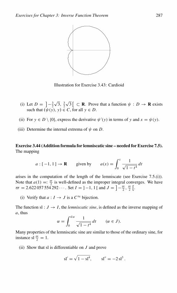
Exercises for Chapter 3: Inverse Function Theorem 287
Illustration for Exercise 3.43: Cardioid
(i) Let D = ]− 32
√3, 3
2
√3[ ⊂ R. Prove that a function ψ : D → R exists
such that (ψ(y), y) ∈ C , for all y ∈ D.
(ii) For y ∈ D \ {0}, express the derivative ψ ′(y) in terms of y and x = ψ(y).
(iii) Determine the internal extrema of ψ on D.
Exercise 3.44 (Addition formula for lemniscatic sine – needed for Exercise 7.5).The mapping
a : [ −1, 1 ] → R given by a(x) =∫ x
0
1√1− t4
dt
arises in the computation of the length of the lemniscate (see Exercise 7.5.(i)).Note that a(1) =: !
2 is well-defined as the improper integral converges. We have! = 2.622 057 554 292 · · · . Set I = ]−1, 1 [ and J = ]−!
2 ,!2
[.
(i) Verify that a : I → J is a C∞ bijection.
The function sl : J → I , the lemniscatic sine, is defined as the inverse mapping ofa, thus
α =∫ sl α
0
1√1− t4
dt (α ∈ J ).
Many properties of the lemniscatic sine are similar to those of the ordinary sine, forinstance sl !2 = 1.
(ii) Show that sl is differentiable on J and prove
sl′ =√
1− sl4, sl′′ = −2 sl3 .
288 Exercises for Chapter 3: Inverse Function Theorem
(iii) Prove that ℘ := sl−2 on J \ {0} satisfies the following differential equation(compare with the Background in Exercise 0.13):
(℘ ′)2 = 4(℘3 − ℘).
We now prove the following addition formula for the lemniscatic sine, valid for α,β and α + β ∈ J ,
sl(α + β) = sl α sl′ β + sl β sl′ α1+ sl2 α sl2 β
.
To this end consider
f : I × I 2 → R with f (x; y, z) = x√
1− y4 + y√
1− x4
1+ x2 y2− z.
(iv) Prove the existence of η, ζ and δ > 0 such that for all y with |y| < η and zwith |z| < ζ there is x = ψ(y) ∈ R with |x | < δ and f (x; y, z) = 0. Verifythat ψ is a C∞ mapping on ]−η, η [× ]−ζ, ζ [.
From now on we treat z as a constant and consider ψ as a function of y alone, witha slight abuse of notation.
(v) Show that the derivative of the mapping ψ : ]−η, η [ → R is given by
ψ ′(y) = −√
1− ψ(y)4√1− y4
, that isψ ′(y)√
1− ψ(y)4+ 1√
1− y4= 0.
Hint:
Dx f (x; y, z) = 1√1− x4
√1− x4
√1− y4(1− x2 y2)− 2xy(x2 + y2)
(1+ x2 y2)2.
(vi) Using the Fundamental Theorem of Integral Calculus and the equalityψ(0) =z deduce ∫ ψ(y)
z
1√1− t4
dt +∫ y
0
1√1− t4
dt = 0,
in other words∫ x
0
1√1− t4
dt +∫ y
0
1√1− t4
dt =∫ z
0
1√1− t4
dt,
z = x√
1− y4 + y√
1− x4
1+ x2 y2.
Applying (ii), verify that the addition formula for the lemniscatic sine is adirect consequence. Note that in Exercise 0.10.(iv) we consider the specialcase of x = y.
Exercises for Chapter 3: Inverse Function Theorem 289
For a second proof of the addition formula introduce new variables γ = α+β2 and
δ = α−β2 , and denote the right–hand side of the addition formula by g(γ, δ).
(vii) Use (ii) to verify ∂g∂δ(γ, δ) = 0 and conclude that g(γ, δ) = g(γ, γ ) for all γ
and δ. The addition formula now follows from g(γ, γ ) = sl 2γ = sl(α+β).(viii) Deduce the following division formula for the lemniscatic sine:
slα
2=
√√√√√1+ sl2 α − 1√1− sl2 α + 1
(0 ≤ α ≤ !
2).
Conclude sl !4 =√√
2− 1 (compare with Exercise 0.10.(iv)).
Hint: Write h(α) =√
1− sl2 α and use the same technique as in part (vii)to verify
h(α + β) = h(α)h(β)− sl α sl β√
1+ sl2 α√
1+ sl2 β
1+ sl2 α sl2 β.
Set a = sl α2 and deduce
h(α) = 1− a2 − a2(1+ a2)
1+ a4= 1− 2a2 − a4
1+ a4.
Finally solve for a2.
Exercise 3.45 (Discriminant locus). In applications of the Implicit Function The-orem 3.5.1 it is often interesting to study the subcollection in the parameter spaceconsisting of the points y ∈ Rp where the condition of the theorem that
Dx f (x; y) ∈ Aut(Rn)
is not met. That is, those y ∈ Rp for which there exists at least one x ∈ Rn suchthat (x, y) ∈ U , f (x; y) = 0, and det Dx f (x; y) = 0. This set is called thediscriminant locus or the bifurcation set.
We now do this for the general quadratic equation
f (x; y) = y2x2 + y1x + y0 (yi ∈ R, 0 ≤ i ≤ 2, y2 = 0).
Prove that the discriminant locus D is given by
D = { y ∈ R3 | y21 − 4y0 y2 = 0 }.
Show that D is a conical surface by substituting y0 = 12 (z2 + z0), y1 = z1, y2 =
12 (z2 − z0). Indeed, we find
D = { z ∈ R3 | z20 + z2
1 − z22 = 0 }.
The complement in R3 of the cone D consists of two disjoint open sets, D+ andD−, made up of points y ∈ R3 for which y2
1 − 4y0 y2 > 0 and < 0, respectively.What we find is that the equation f (x; y) = 0 has two distinct, one, or no solutionx ∈ R depending on whether y ∈ R3 lies in D+, D or D−.
290 Exercises for Chapter 3: Inverse Function Theorem
Exercise 3.46. In thermodynamics one studies real variables P , V and T obeying arelation of the form f (P, V, T ) = 0, for a C1 function f : R3 → R. This relationis used to consider one of the variables, say P , as a function of another, say T , whilekeeping the third variable, V , constant. The notation ∂P
∂T
∣∣V
is used for the derivativeof P with respect to T under constant V . Prove
∂P
∂T
∣∣∣∣V
∂T
∂V
∣∣∣∣P
∂V
∂P
∣∣∣∣T
= −1,
and try to formulate conditions on f for this formula to hold.
Exercise 3.47 (Newtonian mechanics). Let x(t) ∈ Rn be the position at time t ∈ Rof a classical point particle with n degrees of freedom, and assume that t �→ x(t) isa C2 curve in Rn . According to Newton the motion of such a particle is describedby the following second-order differential equation for x :
m x ′′(t) = − grad V (x(t)) (t ∈ R).
Here m > 0 is the mass of the particle and V : Rn → R a C1 function representingthe potential energy of the particle. We define the kinetic energy T : Rn → R andthe total energy E : Rn × Rn → R, respectively, by
T (v) = 1
2m‖v‖2 and E(x, v) = T (v)+ V (x) (v, x ∈ Rn).
(i) Prove that conservation of energy, that is, t �→ E(x(t), x ′(t)) being a constantfunction (equal to E ∈ R, say) on R is equivalent to Newton’s differentialequation.
(ii) From now on suppose n = 1. Verify that in this case x also satisfies afirst-order differential equation
(�) x ′(t) = ±( 2
m(E − V (x(t)))
)1/2,
where one sign only applies. Conclude that x is not uniquely determined ift �→ x(t) is required to be a C1 function satisfying (�).Hint: Consider the situation where x ′(t0) = 0, at some time t0.
(iii) Now assume x ′(t) > 0, for t0 ≤ t ≤ t1. Prove that then V (x) < E , forx(t0) ≤ x ≤ x(t1), and that
t =∫ x(t)
x(t0)
( 2
m(E − V (y))
)−1/2dy.
Prove by means of this result that x(t) is uniquely determined as a functionof x(t0) and E .
Exercises for Chapter 3: Inverse Function Theorem 291
Further assume that a < b; V (a) = V (b) = E ; V (x) < E , for a < x < b;V ′(a) < 0, V ′(b) > 0 (that is, if x(t0) = a, x(t1) = b, then x ′(t0) = x ′(t1) = 0;x ′′(t0) > 0; x ′′(t1) < 0).
(iv) Give a proof that then
T := 2∫ b
a
( 2
m(E − V (x))
)−1/2dx <∞.
Hint: Use, for example, Taylor expansion of x ′(t) in powers of t − t0.
(v) Prove the following. Each motion t �→ x(t) with total energy E which forsome t finds itself in [ a, b ] has the property that x(t) ∈ [ a, b ] for all t ,and, in addition, has a unique continuation for all t ∈ R (being a solution ofNewton’s differential equation). This solution is periodic with period T , i.e.,x(t + T ) = x(t), for all t ∈ R.
Exercise 3.48 (Fundamental Theorem of Algebra – sequel to Exercises 1.7and 1.25). This theorem asserts that for every nonconstant polynomial functionp : C → C there is a z ∈ C with p(z) = 0 (see Example 8.11.5 and Exercise 8.13for other proofs).
(i) Verify that the theorem follows from im(p) = C.
(ii) Using Exercise 1.25 show that im(p) is a closed subset of C.
(iii) Note that the derivative p′ possesses at most finitely many zeros, and concludeby applying the Local Inverse Function Theorem 3.7.1 on C that im(p) hasa nonempty interior.
(iv) Assume that w belongs to the boundary of im(p). Then by (ii) there existsa z ∈ C with p(z) = w. Prove by contradiction, using the Local InverseFunction Theorem on C, that p′(z) = 0. Conclude that the boundary ofim(p) is a finite set.
(v) Prove by means of Exercise 1.7 that im(p) = C.

Exercises for Chapter 4: Manifolds 293
Exercises for Chapter 4
Exercise 4.1. What is the number of degrees of freedom of a bicycle? Assume,for simplicity, that the frame is rigid, that the wheels can rotate about their axes,but cannot wobble, and that both the chain and the pedals are rigidly coupled to therear wheel. What is the number of degrees of freedom when the bicycle rests onthe ground with one or with two wheels, respectively?
Exercise 4.2. Let V ⊂ R2 be the set of points which in polar coordinates (r, α) forR2 satisfy the equation
r = 6
1− 2 cosα.
Show that locally V satisfies: (i) Definition 4.1.3 of zero-set, (ii) Definition 4.1.2 ofparametrized set, and (iii) Definition 4.2.1 of C∞ submanifold in R2 of dimension1. Sketch V .Hint: (i) 3x2
1 + 24x1 − x22 + 36 = 0; (ii) φ(t) = (−4 + 2 cosh t, 2
√3 sinh t),
where cosh t = 12 (e
t + e−t) and sinh t = 12 (e
t − e−t).
Exercise 4.3. Prove that each of the following sets in R2 is a C∞ submanifold inR2 of dimension 1:
{ x ∈ R2 | x2 = x31 }, { x ∈ R2 | x1 = x3
2 }, { x ∈ R2 | x1x2 = 1 };but that this is not the case for the following subsets of R2:
{ x ∈ R2 | x2 = |x1| }, { x ∈ R2 | (x1x2 − 1)(x21 + x2
2 − 2) = 0 },{ x ∈ R2 | x2 = −x2
1 , for x1 ≤ 0; x2 = x21 , for x1 ≥ 0 }.
Why is it that
{ x ∈ R2 | ‖x‖ < 1 } and { x ∈ R2 | |x1| < 1, |x2| < 1 }are submanifolds of R2, but not
{ x ∈ R2 | ‖x‖ ≤ 1 } ?
Exercise 4.4 (Cycloid). (See also Example 5.3.6.) This is the curve φ : R → R2
defined byφ(t) = (t − sin t, 1− cos t).
(i) Prove that φ is an injective C∞ mapping.
(ii) Prove that φ is an immersion at every point t ∈ R with t = 2kπ , for k ∈ Z.
294 Exercises for Chapter 4: Manifolds
Exercise 4.5. Consider the mapping φ : R2 → R3 defined by
φ(α, θ) = (cosα cos θ, sin α cos θ, sin θ).
(i) Prove that φ is a surjection of R2 onto the unit sphere S2 ⊂ R3 with S2 ={ x ∈ R3 | ‖x‖ = 1 }. Describe the inverse image under φ of a point in S2,paying special attention to the points (0, 0, ±1).
(ii) Find the points in R2 where the mapping φ is regular.
(iii) Draw the images of the lines with the equations θ = constant and α =constant, respectively, for different values of θ and α, respectively.
(iv) Determine a maximal open set D ⊂ R2 such that φ : D → S2 is injective.Is φ|D regular on D? And surjective? Is φ : D → φ(D) an embedding?
Exercise 4.6 (Surfaces of revolution – needed for Exercises 5.32 and 6.25).Assume that C is a curve in R3 lying in the half-plane { x ∈ R3 | x1 > 0, x2 = 0 }.Further assume that C = im(γ ) for the Ck embedding γ : I → R3 with
γ (s) = (γ1(s), 0, γ3(s)).
The surface of revolution V formed by revolving C about the x3-axis is defined asV = im(φ) for the mapping φ : I × R → R3 with
φ(s, t) = (γ1(s) cos t, γ1(s) sin t, γ3(s)).
(i) Prove thatφ is injective if the domain ofφ is suitably restricted, and determinea maximal domain with this property.
(ii) Prove that φ is a Ck immersion everywhere (it is useful to note that C doesnot intersect the x3-axis).
(iii) Prove that x = φ(s, t) ∈ V implies that, for t = (2k + 1)π with k ∈ Z,
t = 2 arctan
(x2
x1 +√
x21 + x2
2
),
while for t in a neighborhood of (2k + 1)π with k ∈ Z,
t = 2 arccotan
(x2
−x1 +√
x21 + x2
2
).
Use the fact that φ|D , for a suitably chosen domain D ⊂ R2, is a Ck em-bedding. Prove that the surface of revolution V is a Ck submanifold in R3 ofdimension 2.
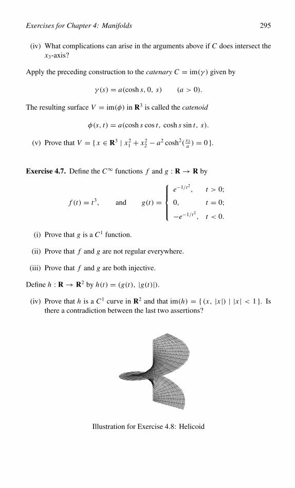
Exercises for Chapter 4: Manifolds 295
(iv) What complications can arise in the arguments above if C does intersect thex3-axis?
Apply the preceding construction to the catenary C = im(γ ) given by
γ (s) = a(cosh s, 0, s) (a > 0).
The resulting surface V = im(φ) in R3 is called the catenoid
φ(s, t) = a(cosh s cos t, cosh s sin t, s).
(v) Prove that V = { x ∈ R3 | x21 + x2
2 − a2 cosh2( x3a ) = 0 }.
Exercise 4.7. Define the C∞ functions f and g : R → R by
f (t) = t3, and g(t) =
e−1/t2
, t > 0;0, t = 0;−e−1/t2
, t < 0.
(i) Prove that g is a C1 function.
(ii) Prove that f and g are not regular everywhere.
(iii) Prove that f and g are both injective.
Define h : R → R2 by h(t) = (g(t), |g(t)|).(iv) Prove that h is a C1 curve in R2 and that im(h) = { (x, |x |) | |x | < 1 }. Is
there a contradiction between the last two assertions?
Illustration for Exercise 4.8: Helicoid
296 Exercises for Chapter 4: Manifolds
Exercise 4.8 (Helix and helicoid – needed for Exercises 5.32 and 7.3). ( �λιξ =curl of hair.) The spiral or helix is the curve in R3 defined by
t �→ (cos t, sin t, at) (a ∈ R+, t ∈ R).
The helicoid is the surface in R3 defined by
(s, t) �→ (s cos t, s sin t, at) ((s, t) ∈ R+ × R).
(i) Prove that the helix and the helicoid are C∞ submanifolds in R3 of dimension1 and 2, respectively. Verify that the helicoid is generated when through everypoint of the helix a line is drawn which intersects the x3-axis and which runsparallel to the plane x3 = 0.
(ii) Prove that a point x of the helicoid satisfies the equation
x2 = x1 tan( x3
a
), when
x3
a/∈
](k + 1
4)π, (k + 3
4)π
[;
x1 = x2 cot( x3
a
), when
x3
a∈
[(k + 1
4)π, (k + 3
4)π
],
where k ∈ Z.
Exercise 4.9 (Closure of embedded submanifold). Define f : R+ → ] 0, 1 [ byf (t) = 2
πarctan t , and consider the mapping φ : R+ → R2, given by φ(t) =
f (t)(cos t, sin t).
(i) Show that φ is a C∞ embedding and conclude that V = φ(R+) is a C∞submanifold in R2 of dimension 1.
(ii) Prove that V is closed in the open subset U = { x ∈ R2 | 0 < ‖x‖ < 1 } ofR2.
(iii) As usual, denote by V the closure of V in R2. Show that V \ V = ∂U .
Background. The closure of an embedded submanifold may be a complicated set,as this example demonstrates.
Exercise 4.10. Let V be a Ck submanifold in Rn of dimension d. Prove that thereexist countably many open sets U in Rn such that V ∩ U is as in Definition 4.2.1and V is contained in the union of those sets V ∩U .
Exercise 4.11. Define g : R2 → R by g(x) = x31 − x3
2 .
(i) Prove that g is a surjective C∞ function.
Exercises for Chapter 4: Manifolds 297
(ii) Prove that g is a C∞ submersion at every point x ∈ R2 \ {0}.(iii) Prove that for all c ∈ R the set { x ∈ R2 | g(x) = c } is a C∞ submanifold in
R2 of dimension 1.
Exercise 4.12. Define g : R3 → R by g(x) = x21 + x2
2 − x23 .
(i) Prove that g is a surjective C∞ function.
(ii) Prove that g is a submersion at every point x ∈ R3 \ {0}.(iii) Prove that the two sheets of the cone
g−1({0}) \ {0} = { x ∈ R3 \ {0} | x21 + x2
2 = x23 }
form a C∞ submanifold in R3 of dimension 2 (compare with Example 4.2.3).
Exercise 4.13. Consider the mappings φi : R2 → R3 (i = 1, 2) defined by
φ1(y) = (ay1 cos y2, by1 sin y2, y21),
φ2(y) = (a sinh y1 cos y2, b sinh y1 sin y2, c cosh y1),
with images equal to an elliptic paraboloid and a hyperboloid of two sheets, respec-tively; here a, b, c > 0.
(i) Establish at which points of R2 the mapping φi is regular.
(ii) Determine Vi = im(φi ), and prove that Vi is a C∞ manifold in R3 of dimen-sion 2.Hint: Recall the Submersion Theorem 4.5.2.
Exercise 4.14 (Quadrics – needed for Exercises 5.6 and 5.12). A nondegeneratequadric in Rn is a set having the form
V = { x ∈ Rn | 〈Ax, x〉 + 〈b, x〉 + c = 0 },where A ∈ End+(Rn) ∩ Aut(Rn), b ∈ Rn and c ∈ R. Introduce the discriminant� = 〈b, A−1b〉 − 4c ∈ R.
(i) Prove that V is an (n − 1)-dimensional C∞ submanifold of Rn , provided� = 0.
(ii) Suppose � = 0. Prove that − 12 A−1b ∈ V and that W = V \ {− 1
2 A−1b }always is an (n − 1)-dimensional C∞ submanifold of Rn .
(iii) Now assume that A is positive definite. Use the substitution of variablesx = y − 1
2 A−1b to prove the following. If � < 0, then V = ∅; if � = 0,then V = {− 1
2 A−1b } and W = ∅; and if � > 0, then V is an ellipsoid.
298 Exercises for Chapter 4: Manifolds
Exercise 4.15 (Needed for Exercise 4.16). Let 1 ≤ d ≤ n, and let there be givenvectors a(1), . . . , a(d) ∈ Rn and numbers r1, . . . , rd ∈ R. Let x0 ∈ Rn such that‖x0− a(i)‖ = ri , for 1 ≤ i ≤ d. Prove by means of the Submersion Theorem 4.5.2that at x0
V = { x ∈ Rn | ‖x − a(i)‖ = ri (1 ≤ i ≤ d) }is a C∞ manifold in Rn of codimension d, under the assumption that the vectorsx0 − a(1), . . . , x0 − a(d) form a linearly independent system in Rn .
Exercise 4.16 (Sequel to Exercise 4.15). For Exercise 4.15 it is also possible togive a fully explicit solution: by induction over d ≤ n one can prove that in thecase when the vectors a(1) − a(2), . . . , a(1) − a(d) are linearly independent, the setV equals
{ x ∈ Hd | ‖x − b(d)‖2 = sd },where b(d) ∈ Hd , sd ∈ R, and
Hd = { x ∈ Rn | 〈x, a(1) − a(i)〉 = c j , for all i = 2, . . . , d }
is a plane of dimension n − d + 1 in Rn . If sd > 0 we therefore obtain an (n − d)-dimensional sphere with radius
√sd in Hd ; if sd = 0, a point; and if sd < 0, the
empty set. In particular: if d = n, V consists of two points at most. First try toverify the assertions for d = 2. Pay particular attention also to what may happenin the case n = 3.
Exercise 4.17 (Lines on hyperboloid of one sheet). Consider the hyperboloid ofone sheet in R3
V = { x ∈ R3 | x21
a2+ x2
2
b2− x2
3
c2= 1 } (a, b, c > 0).
Note that for x ∈ V ,( x1
a+ x3
c
)( x1
a− x3
c
)=
(1+ x2
b
)(1− x2
b
).
(i) From this, show that through every point of V run two different straight linesthat lie entirely on V , and that thus one finds two one-parameter families ofstraight lines lying entirely on V .
(ii) Prove that two different lines from one family do not intersect and are non-parallel.
(iii) Prove that two lines from different families either intersect or are parallel.
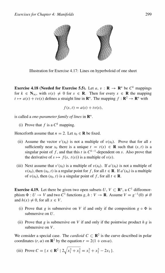
Exercises for Chapter 4: Manifolds 299
Illustration for Exercise 4.17: Lines on hyperboloid of one sheet
Exercise 4.18 (Needed for Exercise 5.5). Let a, v : R → Rn be Ck mappingsfor k ∈ N∞, with v(s) = 0 for s ∈ R. Then for every s ∈ R the mappingt �→ a(s)+ tv(s) defines a straight line in Rn . The mapping f : R2 → Rn with
f (s, t) = a(s)+ tv(s),
is called a one-parameter family of lines in Rn .
(i) Prove that f is a Ck mapping.
Henceforth assume that n = 2. Let s0 ∈ R be fixed.
(ii) Assume the vector v′(s0) is not a multiple of v(s0). Prove that for all ssufficiently near s0 there is a unique t = t (s) ∈ R such that (s, t) is asingular point of f , and that this t is Ck−1-dependent on s. Also prove thatthe derivative of s �→ f (s, t (s)) is a multiple of v(s).
(iii) Next assume that v′(s0) is a multiple of v(s0). If a′(s0) is not a multiple ofv(s0), then (s0, t) is a regular point for f , for all t ∈ R. If a′(s0) is a multipleof v(s0), then (s0, t) is a singular point of f , for all t ∈ R.
Exercise 4.19. Let there be given two open subsets U , V ⊂ Rn , a C1 diffeomor-phism � : U → V and two C1 functions g, h : V → R. Assume V = g−1(0) = ∅and h(x) = 0, for all x ∈ V .
(i) Prove that g is submersive on V if and only if the composition g ◦ � issubmersive on U .
(ii) Prove that g is submersive on V if and only if the pointwise product h g issubmersive on V .
We consider a special case. The cardioid C ⊂ R2 is the curve described in polarcoordinates (r, α) on R2 by the equation r = 2(1+ cosα).
(iii) Prove C = { x ∈ R2 | 2√
x21 + x2
2 = x21 + x2
2 − 2x1 }.
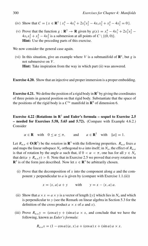
300 Exercises for Chapter 4: Manifolds
(iv) Show that C = { x ∈ R2 | x41 − 4x3
1 + 2x21 x2
2 − 4x1x22 + x4
2 − 4x22 = 0 }.
(v) Prove that the function g : R2 → R given by g(x) = x41 − 4x3
1 + 2x21 x2
2 −4x1x2
2 + x42 − 4x2
2 is a submersion at all points of C \ {(0, 0)}.Hint: Use the preceding parts of this exercise.
We now consider the general case again.
(vi) In this situation, give an example where V is a submanifold of Rn , but g isnot submersive on V .Hint: Take inspiration from the way in which part (ii) was answered.
Exercise 4.20. Show that an injective and proper immersion is a proper embedding.
Exercise 4.21. We define the position of a rigid body in R3 by giving the coordinatesof three points in general position on that rigid body. Substantiate that the space ofthe positions of the rigid body is a C∞ manifold in R9 of dimension 6.
Exercise 4.22 (Rotations in R3 and Euler’s formula – sequel to Exercise 2.5– needed for Exercises 5.58, 5.65 and 5.72). (Compare with Example 4.6.2.)Consider
α ∈ R with 0 ≤ α ≤ π, and a ∈ R3 with ‖a‖ = 1.
Let Rα,a ∈ O(R3) be the rotation in R3 with the following properties. Rα,a fixes aand maps the linear subspace Na orthogonal to a into itself; in Na , the effect of Rα,a
is that of rotation by the angle α such that, if 0 < α < π , one has for all y ∈ Na
that det(a y Rα,a y) > 0. Note that in Exercise 2.5 we proved that every rotation inR3 is of the form just described. Now let x ∈ R3 be arbitrarily chosen.
(i) Prove that the decomposition of x into the component along a and the com-ponent y perpendicular to a is given by (compare with Exercise 1.1.(ii))
x = 〈x, a〉 a + y with y = x − 〈x, a〉 a.
(ii) Show that a× x = a× y is a vector of length ‖y‖which lies in Na and whichis perpendicular to y (see the Remark on linear algebra in Section 5.3 for thedefinition of the cross product a × x of a and x).
(iii) Prove Rα,a y = (cosα) y + (sin α) a × x , and conclude that we have thefollowing, known as Euler’s formula:
Rα,a x = (1− cosα)〈a, x〉 a + (cosα) x + (sin α) a × x .
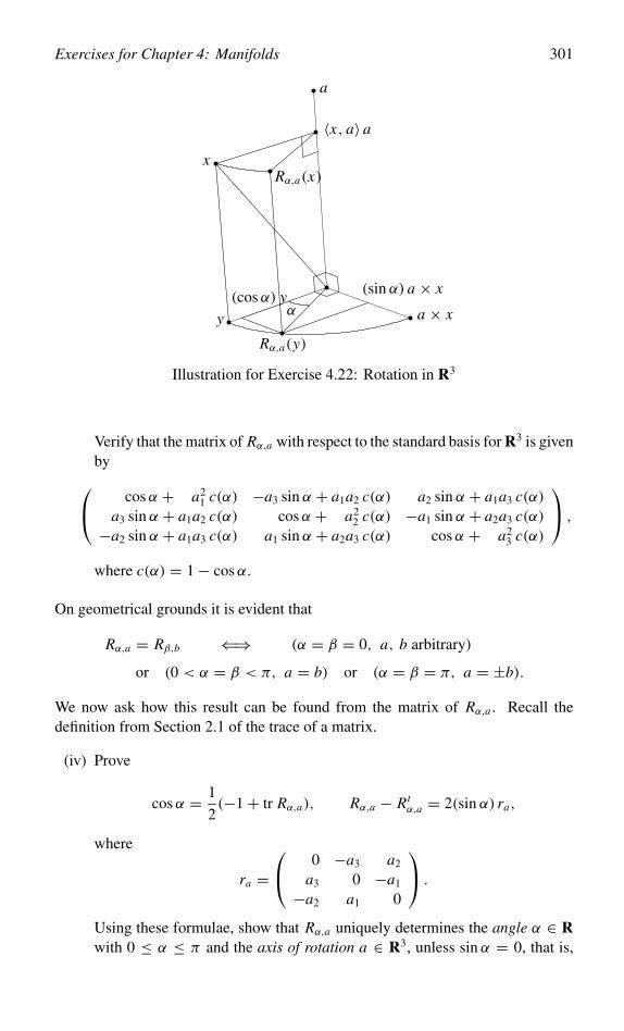
Exercises for Chapter 4: Manifolds 301
a
x
〈x, a〉 a
Rα,a(x)
y
(cosα) yα
Rα,a(y)
a × x
(sin α) a × x
Illustration for Exercise 4.22: Rotation in R3
Verify that the matrix of Rα,a with respect to the standard basis for R3 is givenby cosα + a2
1 c(α) −a3 sin α + a1a2 c(α) a2 sin α + a1a3 c(α)a3 sin α + a1a2 c(α) cosα + a2
2 c(α) −a1 sin α + a2a3 c(α)−a2 sin α + a1a3 c(α) a1 sin α + a2a3 c(α) cosα + a2
3 c(α)
,
where c(α) = 1− cosα.
On geometrical grounds it is evident that
Rα,a = Rβ,b ⇐⇒ (α = β = 0, a, b arbitrary)
or (0 < α = β < π, a = b) or (α = β = π, a = ±b).
We now ask how this result can be found from the matrix of Rα,a . Recall thedefinition from Section 2.1 of the trace of a matrix.
(iv) Prove
cosα = 1
2(−1+ tr Rα,a), Rα,a − Rt
α,a = 2(sin α) ra,
where
ra = 0 −a3 a2
a3 0 −a1
−a2 a1 0
.
Using these formulae, show that Rα,a uniquely determines the angle α ∈ Rwith 0 ≤ α ≤ π and the axis of rotation a ∈ R3, unless sin α = 0, that is,
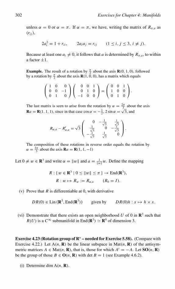
302 Exercises for Chapter 4: Manifolds
unless α = 0 or α = π . If α = π , we have, writing the matrix of Rπ,a as(ri j ),
2a2i = 1+ rii , 2ai a j = ri j (1 ≤ i, j ≤ 3, i = j).
Because at least one ai = 0, it follows that a is determined by Rπ,a , to withina factor ±1.
Example. The result of a rotation by π2 about the axis R(0, 1, 0), followed
by a rotation by π2 about the axis R(1, 0, 0), has a matrix which equals 1 0 0
0 0 −10 1 0
0 0 10 1 0−1 0 0
= 0 0 1
1 0 00 1 0
.
The last matrix is seen to arise from the rotation by α = 2π3 about the axis
Ra = R(1, 1, 1), since in that case cosα = − 12 , 2 sin α = √3, and
Rα,a − Rtα,a =
√3
0 − 1√3
1√3
1√3
0 − 1√3
− 1√3
1√3
0
.
The composition of these rotations in reverse order equals the rotation byα = 2π
3 about the axis Ra = R(1, 1,−1)
Let 0 = w ∈ R3 and write α = ‖w‖ and a = 1‖w‖w. Define the mapping
R : {w ∈ R3 | 0 ≤ ‖w‖ ≤ π } → End(R3),
R : w �→ Rw := Rα,a (R0 = I ).
(v) Prove that R is differentiable at 0, with derivative
DR(0) ∈ Lin (R3,End(R3)) given by DR(0)h : x �→ h × x .
(vi) Demonstrate that there exists an open neighborhood U of 0 in R3 such thatR(U ) is a C∞ submanifold in End(R3) � R9 of dimension 3.
Exercise 4.23 (Rotation group of Rn – needed for Exercise 5.58). (Compare withExercise 4.22.) Let A(n,R) be the linear subspace in Mat(n,R) of the antisym-metric matrices A ∈ Mat(n,R), that is, those for which At = −A. Let SO(n,R)be the group of those B ∈ O(n,R) with det B = 1 (see Example 4.6.2).
(i) Determine dim A(n,R).
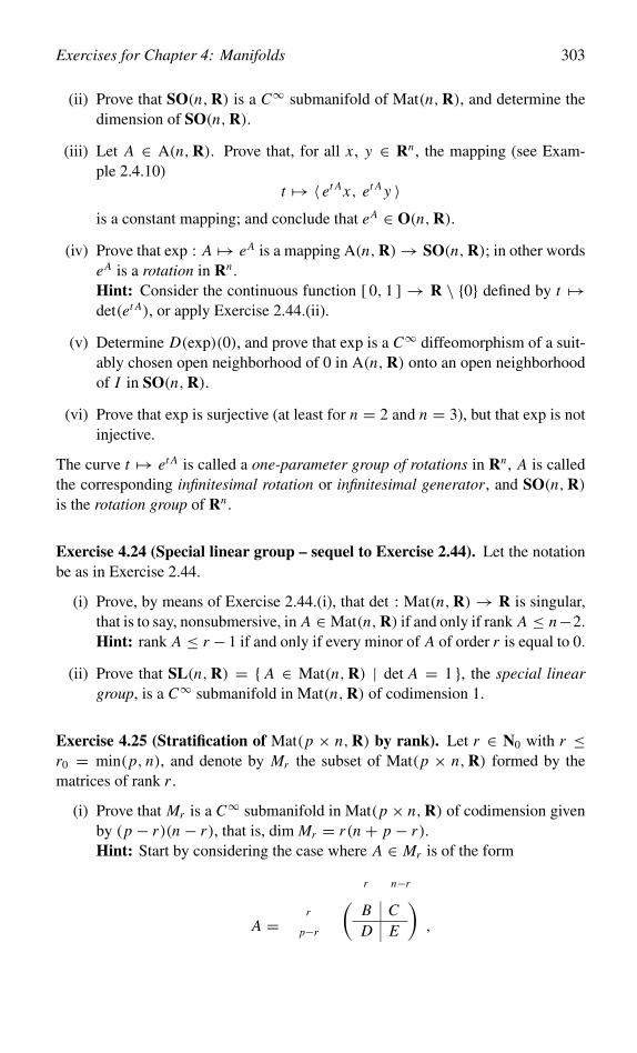
Exercises for Chapter 4: Manifolds 303
(ii) Prove that SO(n,R) is a C∞ submanifold of Mat(n,R), and determine thedimension of SO(n,R).
(iii) Let A ∈ A(n,R). Prove that, for all x , y ∈ Rn , the mapping (see Exam-ple 2.4.10)
t �→ 〈 et Ax, et A y 〉is a constant mapping; and conclude that eA ∈ O(n,R).
(iv) Prove that exp : A �→ eA is a mapping A(n,R)→ SO(n,R); in other wordseA is a rotation in Rn .Hint: Consider the continuous function [ 0, 1 ] → R \ {0} defined by t �→det(et A), or apply Exercise 2.44.(ii).
(v) Determine D(exp)(0), and prove that exp is a C∞ diffeomorphism of a suit-ably chosen open neighborhood of 0 in A(n,R) onto an open neighborhoodof I in SO(n,R).
(vi) Prove that exp is surjective (at least for n = 2 and n = 3), but that exp is notinjective.
The curve t �→ et A is called a one-parameter group of rotations in Rn , A is calledthe corresponding infinitesimal rotation or infinitesimal generator, and SO(n,R)is the rotation group of Rn .
Exercise 4.24 (Special linear group – sequel to Exercise 2.44). Let the notationbe as in Exercise 2.44.
(i) Prove, by means of Exercise 2.44.(i), that det : Mat(n,R)→ R is singular,that is to say, nonsubmersive, in A ∈ Mat(n,R) if and only if rank A ≤ n−2.Hint: rank A ≤ r − 1 if and only if every minor of A of order r is equal to 0.
(ii) Prove that SL(n,R) = { A ∈ Mat(n,R) | det A = 1 }, the special lineargroup, is a C∞ submanifold in Mat(n,R) of codimension 1.
Exercise 4.25 (Stratification of Mat(p × n,R) by rank). Let r ∈ N0 with r ≤r0 = min(p, n), and denote by Mr the subset of Mat(p × n,R) formed by thematrices of rank r .
(i) Prove that Mr is a C∞ submanifold in Mat(p × n,R) of codimension givenby (p − r)(n − r), that is, dim Mr = r(n + p − r).Hint: Start by considering the case where A ∈ Mr is of the form
A =
r n−r
r
p−r
(B CD E
),
304 Exercises for Chapter 4: Manifolds
with B ∈ GL(r,R). Then multiply from the right by the following matrix inGL(n,R): (
I −B−1C0 I
),
to prove that rank A = r if and only if E − DB−1C = 0. Deduce that Mr
near A equals the graph of (B,C, D) �→ DB−1C .
(ii) Show that r �→ dim Mr is monotonically increasing on [ 0, r0 ]. Verify thatdim Mr0 = pn and deduce that Mr0 is an open subset of Mat(p × n,R).
(iii) Prove that the set { A ∈ Mat(p × n,R) | rank A ≤ r } is given by thevanishing of polynomial functions: all the minors of A of order r + 1 haveto vanish. Deduce that this subset is closed in Mat(p × n,R), and that theclosure of Mr is the union of the Mr ′ with 0 ≤ r ′ ≤ r . Conclude that{ A ∈ Mat(p×n,R) | rank A ≥ r } is open, because its complement is givenby the condition rank A ≤ r − 1. Let A ∈ Mat(p × n,R), and show thatrank A′ ≥ rank A, for every A′ ∈ Mat(p × n,R) sufficiently close to A.
Background. E−DB−1C is called the Schur complement of B in A, and is denotedby (A|B). We have det A = det B det(A|B). Above we obtained what is called astratification: the “singular” object under consideration, which is here the closureof Mr , has the form of a finite union of strata each of which is a submanifold, withthe closure of each of these strata being in turn composed of the stratum itself andstrata of lower dimensions.
Exercise 4.26 (Hopf fibration and stereographic projection – needed for Ex-ercises 5.68 and 5.70). Let x ∈ R4, and write α = α(x) = x1 + i x4 andβ = β(x) = x3 + i x2 ∈ C (where i = √−1). This gives an identification ofR4 with C2 via x ↔ (α(x), β(x)). Define g : R4 → R3 by (compare with the lastcolumn in the matrix in Exercise 5.66.(vi))
g(x) = g(α, β) = 2 Re(αβ)
2 Im(αβ)
|α|2 − |β|2
= 2(x2x4 + x1x3)
2(x3x4 − x1x2)
x21 − x2
2 − x23 + x2
4
.
(i) Prove that g is a submersion on R4 \ {0}.Hint: We have
Dg(x) = 2
x3 x4 x1 x2
−x2 −x1 x4 x3
x1 −x2 −x3 x4
.
The row vectors in this matrix all have length 2‖x‖ and are mutually orthogo-nal in R4. Or else, let M j be the matrix obtained from Dg(x) by deleting thecolumn which does not contain x j . Then det M j = 8x j‖x‖2, for 1 ≤ j ≤ 4.
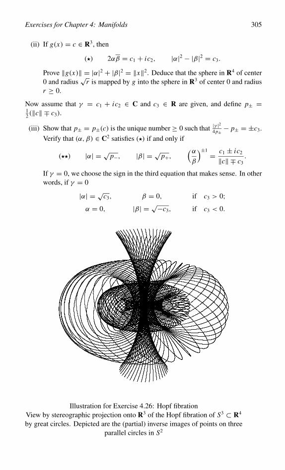
Exercises for Chapter 4: Manifolds 305
(ii) If g(x) = c ∈ R3, then
(�) 2αβ = c1 + ic2, |α|2 − |β|2 = c3.
Prove ‖g(x)‖ = |α|2 + |β|2 = ‖x‖2. Deduce that the sphere in R4 of center0 and radius
√r is mapped by g into the sphere in R3 of center 0 and radius
r ≥ 0.
Now assume that γ = c1 + ic2 ∈ C and c3 ∈ R are given, and define p± =12 (‖c‖ ∓ c3).
(iii) Show that p± = p±(c) is the unique number≥ 0 such that |γ |2
4p± − p± = ±c3.
Verify that (α, β) ∈ C2 satisfies (�) if and only if
(��) |α| = √p−, |β| = √p+,(αβ
)±1 = c1 ± ic2
‖c‖ ∓ c3.
If γ = 0, we choose the sign in the third equation that makes sense. In otherwords, if γ = 0
|α| = √c3, β = 0, if c3 > 0;α = 0, |β| = √−c3, if c3 < 0.
Illustration for Exercise 4.26: Hopf fibrationView by stereographic projection onto R3 of the Hopf fibration of S3 ⊂ R4
by great circles. Depicted are the (partial) inverse images of points on threeparallel circles in S2
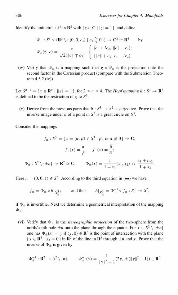
306 Exercises for Chapter 4: Manifolds
Identify the unit circle S1 in R2 with { z ∈ C | |z| = 1 }, and define
�± : S1 × (R3 \ { (0, 0, c3) | c3 � 0 })→ C2 � R4 by
�±(z, c) = z√2(‖c‖ ∓ c3)
·{(c1 + ic2, ‖c‖ − c3);(‖c‖ + c3, c1 − ic2).
(iv) Verify that �± is a mapping such that g ◦ �± is the projection onto thesecond factor in the Cartesian product (compare with the Submersion Theo-rem 4.5.2.(iv)).
Let Sn−1 = { x ∈ Rn | ‖x‖ = 1 }, for 2 ≤ n ≤ 4. The Hopf mapping h : S3 → R3
is defined to be the restriction of g to S3.
(v) Derive from the previous parts that h : S3 → S2 is surjective. Prove that theinverse image under h of a point in S2 is a great circle on S3.
Consider the mappings
f± : S3± = { x = (α, β) ∈ S3 | β, or α = 0 } → C,
f+(x) = α
β, f−(x) = β
α;
�± : S2 \ {±n} → R2 � C, �±(x) = 1
1∓ x3(x1, x2)↔ x1 + i x2
1∓ x3.
Here n = (0, 0, 1) ∈ S2. According to the third equation in (��) we have
f± = �± ◦ h|S3±; and thus h|S3±
= �−1± ◦ f± : S3
± → S2,
if �± is invertible. Next we determine a geometrical interpretation of the mapping�±.
(vi) Verify that �± is the stereographic projection of the two-sphere from thenorth/south pole ±n onto the plane through the equator. For x ∈ S2 \ {±n}one has �±(x) = y if (y, 0) ∈ R3 is the point of intersection with the plane{ x ∈ R3 | x3 = 0 } in R3 of the line in R3 through ±n and x . Prove that theinverse of �± is given by
�−1± : R2 → S2 \ {n}, �−1
± (y) = 1
‖y‖2 + 1(2y, ±(‖y‖2 − 1)) ∈ R3.
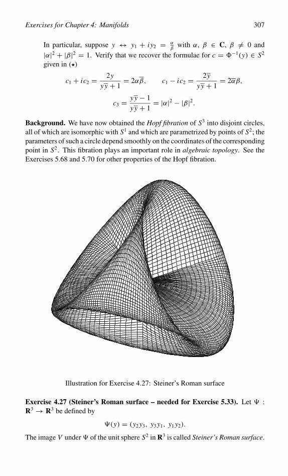
Exercises for Chapter 4: Manifolds 307
In particular, suppose y ↔ y1 + iy2 = αβ
with α, β ∈ C, β = 0 and
|α|2 + |β|2 = 1. Verify that we recover the formulae for c = �−1(y) ∈ S2
given in (�)
c1 + ic2 = 2y
yy + 1= 2αβ, c1 − ic2 = 2y
yy + 1= 2αβ,
c3 = yy − 1
yy + 1= |α|2 − |β|2.
Background. We have now obtained the Hopf fibration of S3 into disjoint circles,all of which are isomorphic with S1 and which are parametrized by points of S2; theparameters of such a circle depend smoothly on the coordinates of the correspondingpoint in S2. This fibration plays an important role in algebraic topology. See theExercises 5.68 and 5.70 for other properties of the Hopf fibration.
Illustration for Exercise 4.27: Steiner’s Roman surface
Exercise 4.27 (Steiner’s Roman surface – needed for Exercise 5.33). Let � :R3 → R3 be defined by
�(y) = (y2 y3, y3 y1, y1 y2).
The image V under� of the unit sphere S2 in R3 is called Steiner’s Roman surface.
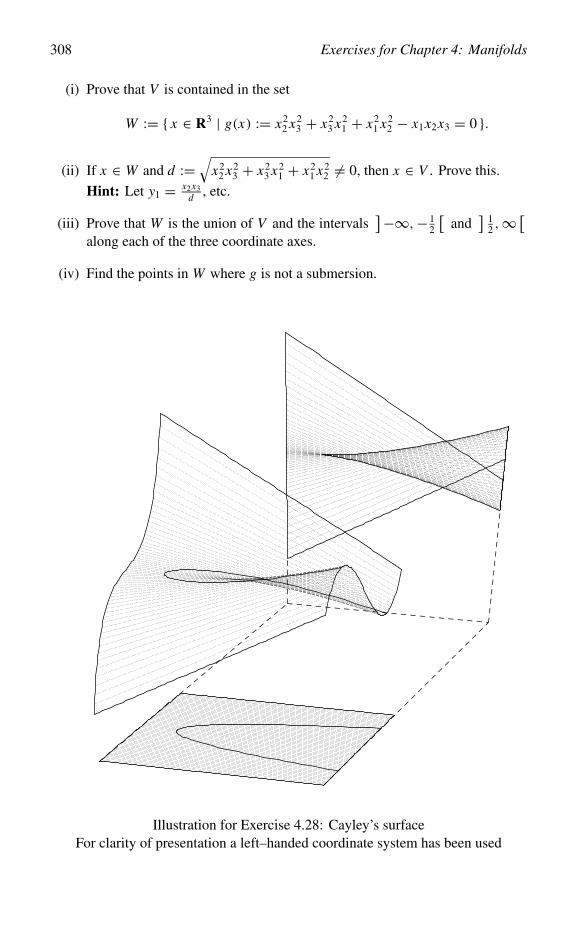
308 Exercises for Chapter 4: Manifolds
(i) Prove that V is contained in the set
W := { x ∈ R3 | g(x) := x22 x2
3 + x23 x2
1 + x21 x2
2 − x1x2x3 = 0 }.
(ii) If x ∈ W and d :=√
x22 x2
3 + x23 x2
1 + x21 x2
2 = 0, then x ∈ V . Prove this.
Hint: Let y1 = x2x3d , etc.
(iii) Prove that W is the union of V and the intervals]−∞,− 1
2
[and
]12 ,∞
[along each of the three coordinate axes.
(iv) Find the points in W where g is not a submersion.
Illustration for Exercise 4.28: Cayley’s surfaceFor clarity of presentation a left–handed coordinate system has been used
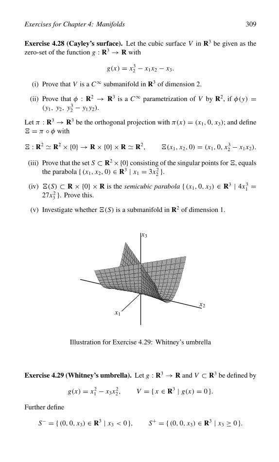
Exercises for Chapter 4: Manifolds 309
Exercise 4.28 (Cayley’s surface). Let the cubic surface V in R3 be given as thezero-set of the function g : R3 → R with
g(x) = x32 − x1x2 − x3.
(i) Prove that V is a C∞ submanifold in R3 of dimension 2.
(ii) Prove that φ : R2 → R3 is a C∞ parametrization of V by R2, if φ(y) =(y1, y2, y3
2 − y1 y2).
Let π : R3 → R3 be the orthogonal projection with π(x) = (x1, 0, x3); and define� = π ◦ φ with
� : R2 � R2 × {0} → R× {0} ×R � R2, �(x1, x2, 0) = (x1, 0, x32 − x1x2).
(iii) Prove that the set S ⊂ R2×{0} consisting of the singular points for�, equalsthe parabola { (x1, x2, 0) ∈ R3 | x1 = 3x2
2 }.(iv) �(S) ⊂ R × {0} × R is the semicubic parabola { (x1, 0, x3) ∈ R3 | 4x3
1 =27x2
3 }. Prove this.
(v) Investigate whether �(S) is a submanifold in R2 of dimension 1.
x1
x2
x3
Illustration for Exercise 4.29: Whitney’s umbrella
Exercise 4.29 (Whitney’s umbrella). Let g : R3 → R and V ⊂ R3 be defined by
g(x) = x21 − x3x2
2 , V = { x ∈ R3 | g(x) = 0 }.Further define
S− = { (0, 0, x3) ∈ R3 | x3 < 0 }, S+ = { (0, 0, x3) ∈ R3 | x3 ≥ 0 }.
310 Exercises for Chapter 4: Manifolds
(i) Prove that V is a C∞ submanifold in R3 at each point x ∈ V \ (S− ∪ S+),and determine the dimension of V at each of these points x .
(ii) Verify that the x2-axis and the x3-axis are both contained in V . Also provethat V is a C∞ submanifold in R3 of dimension 1 at every point x ∈ S−.
(iii) Intersect V with the plane { (x1, y1, x3) ∈ R3 | (x1, x3) ∈ R2 }, for everyy1 ∈ R, and show that V \ S− = im(φ), where φ : R2 → R3 is defined byφ(y) = (y1 y2, y1, y2
2).
(iv) Prove that φ : R2 \ { (0, y2) ∈ R2 | y2 ∈ R } → R3 \ S+ is an embedding.
(v) Prove that V is not a C0 submanifold in R3 at the point x if x ∈ S+.Hint: Intersect V with the plane { (x1, x2, x3) ∈ R3 | (x1, x2) ∈ R2 }.
Exercise 4.30 (Submersions are locally determined by one image point). Letxi in Rn and gi : Rn → Rn−d be C1 mappings, for i = 1, 2. Assume thatg1(x1) = g2(x2) and that gi is a submersion at xi , for i = 1, 2. Prove that thereexist open neighborhoods Ui of xi , for i = 1, 2, in Rn and a C1 diffeomorphism� : U1 → U2 such that
�(x1) = x2 and g1 = g2 ◦�.
Exercise 4.31 (Analog of Hilbert’s Nullstellensatz – needed for Exercises 4.32and 5.74).
(i) Let g : R → R be given by g(x) = x ; then V := { x ∈ R | g(x) = 0 } = {0}.Assume that f : R → R is a C∞ function such that f (x) = 0, for x ∈ V ,that is, f (0) = 0. Then prove that there exists a C∞ function f1 : R → Rsuch that for all x ∈ R,
f (x) = x f1(x) = f1(x) g(x).
Hint: f (x)− f (0) = ∫ 10
d fdt (t x) dt = x
∫ 10 f ′(t x) dt .
(ii) Let U0 ⊂ Rn be an open subset, let g : U0 → Rn−d be a C∞ submersion,and define V := { x ∈ U0 | g(x) = 0 }. Assume that f : U0 → R isa C∞ function such that f (x) = 0, for all x ∈ V . Then prove that, forevery x0 ∈ U0, there exist a neighborhood U of x0 in U0, and C∞ functionsfi : U → R, with 1 ≤ i ≤ n − d, such that for all x ∈ U ,
f (x) = f1(x)g1(x)+ · · · + fn−d(x)gn−d(x).
Hint: Let x = �(y, c) be the substitution of variables from assertion (iv) of
Exercises for Chapter 4: Manifolds 311
the Submersion Theorem 4.5.2, with (y, c) ∈ W := �(U ) ⊂ Rd × Rn−d .In particular then, for all (y, c) ∈ W , one has gi (�(y, c)) = ci , for 1 ≤ i ≤n − d. It follows that for every C∞ function h : W → R,
h(y, c)− h(y, 0) =∫ 1
0
dh
dt(y, tc) dt =
∑1≤i≤n−d
ci
∫ 1
0Dd+i h(y, tc) dt
=∑
1≤i≤n−d
gi (�(y, c)) hi (y, c).
Reformulation of (ii). The C∞ functions f : U0 → R form a ring R under theoperations of pointwise addition and multiplication. The collection of the f ∈ Rwith the property f |V = 0 forms an ideal I in R. The result above asserts that theideal I is generated by the functions g1, . . . , gn−d , in a local sense at least.
(iii) Generally speaking, the functions fi from (ii) are not uniquely determined.Verify this, taking the example where g : R3 → R2 is given by g(x) =(x1, x2) and f (x) := x1x3+x2
2 . Note f (x) = (x3−x2)g1(x)+(x1+x2)g2(x).
(iv) Let V := { x ∈ R2 | g(x) := x22 = 0 }. The function f (x) = x2 vanishes for
every x ∈ V . Even so, there do not exist for every x ∈ R2 a neighborhoodU of x and a C∞ function f1 : U → R such that for all x ∈ U we havef (x) = f1(x)g(x). Verify that this is not in contradiction with the assertionfrom (ii).
Background. Note that in the situation of part (iv) there does exist a C∞ functionf1 such that f 2(x) = f1(x)g(x), for all x ∈ R2. In the context of polynomialfunctions one has, in the case when the vectors grad gi (x), for 1 ≤ i ≤ n − d andx ∈ V , are not known to be linearly independent, the following, known as Hilbert’sNullstellensatz.1 Write C[x] for the ring of polynomials in the variables x1, . . . , xn
with coefficients in C. Assume that f, g1, . . . , gc ∈ C[x] and let V := { x ∈ Cn |gi (x) = 0 (1 ≤ i ≤ c) }. If f |V = 0, then there exists a number m ∈ N such thatf m belongs to the ideal in C[x] generated by g1, . . . , gc.
Exercise 4.32 (Analog of de l’Hôpital’s rule – sequel to Exercise 4.31). We usethe notation and the results of Exercise 4.31.(ii). We consider the special case wheredim V = n − 1 and will now investigate to what extent the C∞ submersion g :U0 → R near x0 ∈ V is determined by the set V = { x ∈ U0 | g(x) = 0 }. Assumethat g : U0 → R is a C∞ submersion for which also V = { x ∈ U0 | g(x) = 0 }.Then we have that g(x) = 0, for all x ∈ V . Hence we find a neighborhood U of x0
in U0 and a C∞ function f : U → R such that for all x ∈ U ,
g(x) = f (x)g(x).
1A proof can be found on p. 380 in Lang, S.: Algebra. Addison-Wesley Publishing Company,Reading 1993, or Peter May, J.: Munshi’s proof of the Nullstellensatz. Amer. Math. Monthly 110(2003), 133 – 140.
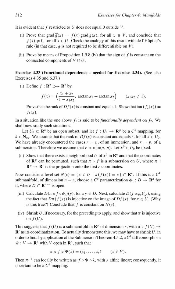
312 Exercises for Chapter 4: Manifolds
It is evident that f restricted to U does not equal 0 outside V .
(i) Prove that grad g(x) = f (x) grad g(x), for all x ∈ V , and conclude thatf (x) = 0, for all x ∈ U . Check the analogy of this result with de l’Hôpital’srule (in that case, g is not required to be differentiable on V ).
(ii) Prove by means of Proposition 1.9.8.(iv) that the sign of f is constant on theconnected components of V ∩U .
Exercise 4.33 (Functional dependence – needed for Exercise 4.34). (See alsoExercises 4.35 and 6.37.)
(i) Define f : R2 ⊃→ R2 by
f (x) =( x1 + x2
1− x1x2, arctan x1 + arctan x2
)(x1x2 = 1).
Prove that the rank of D f (x) is constant and equals 1. Show that tan ( f2(x)) =f1(x).
In a situation like the one above f1 is said to be functionally dependent on f2. Weshall now study such situations.
Let U0 ⊂ Rn be an open subset, and let f : U0 → Rp be a Ck mapping, fork ∈ N∞. We assume that the rank of D f (x) is constant and equals r , for all x ∈ U0.We have already encountered the cases r = n, of an immersion, and r = p, of asubmersion. Therefore we assume that r < min(n, p). Let x0 ∈ U0 be fixed.
(ii) Show that there exists a neighborhood U of x0 in Rn and that the coordinatesof Rp can be permuted, such that π ◦ f is a submersion on U , where π :Rp → Rr is the projection onto the first r coordinates.
Now consider a level set N (c) = { x ∈ U | π( f (x)) = c } ⊂ Rn . If this is a Ck
submanifold, of dimension n − r , choose a Ck parametrization φc : D → Rn forit, where D ⊂ Rn−r is open.
(iii) Calculate D(π ◦ f ◦φc)(y), for a y ∈ D. Next, calculate D( f ◦φc)(y), usingthe fact that Dπ( f (x)) is injective on the image of D f (x), for x ∈ U . (Whyis this true?) Conclude that f is constant on N (c).
(iv) Shrink U , if necessary, for the preceding to apply, and show that π is injectiveon f (U ).
This suggests that f (U ) is a submanifold in R p of dimension r , with π : f (U )→Rr as its coordinatization. To actually demonstrate this, we may have to shrink U , inorder to find, by application of the Submersion Theorem 4.5.2, a Ck diffeomorphism� : V → Rn with V open in Rn , such that
π ◦ f ◦�(x) = (x1, . . . , xr ) (x ∈ V ).
Then π−1 can locally be written as f ◦� ◦ λ, with λ affine linear; consequently, itis certain to be a Ck mapping.
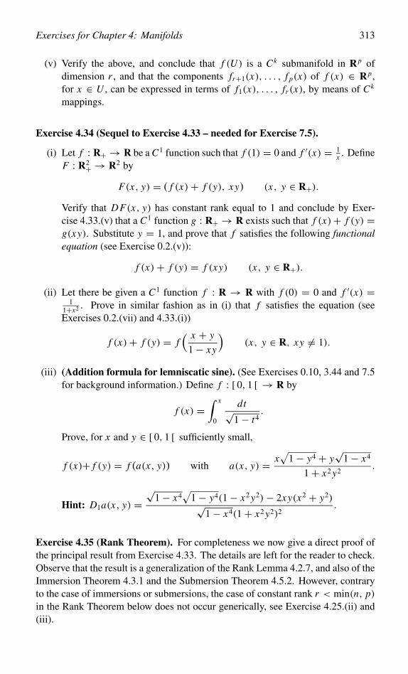
Exercises for Chapter 4: Manifolds 313
(v) Verify the above, and conclude that f (U ) is a Ck submanifold in Rp ofdimension r , and that the components fr+1(x), . . . , f p(x) of f (x) ∈ Rp,for x ∈ U , can be expressed in terms of f1(x), . . . , fr (x), by means of Ck
mappings.
Exercise 4.34 (Sequel to Exercise 4.33 – needed for Exercise 7.5).
(i) Let f : R+ → R be a C1 function such that f (1) = 0 and f ′(x) = 1x . Define
F : R2+ → R2 by
F(x, y) = ( f (x)+ f (y), xy) (x, y ∈ R+).
Verify that DF(x, y) has constant rank equal to 1 and conclude by Exer-cise 4.33.(v) that a C1 function g : R+ → R exists such that f (x)+ f (y) =g(xy). Substitute y = 1, and prove that f satisfies the following functionalequation (see Exercise 0.2.(v)):
f (x)+ f (y) = f (xy) (x, y ∈ R+).
(ii) Let there be given a C1 function f : R → R with f (0) = 0 and f ′(x) =1
1+x2 . Prove in similar fashion as in (i) that f satisfies the equation (seeExercises 0.2.(vii) and 4.33.(i))
f (x)+ f (y) = f( x + y
1− xy
)(x, y ∈ R, xy = 1).
(iii) (Addition formula for lemniscatic sine). (See Exercises 0.10, 3.44 and 7.5for background information.) Define f : [ 0, 1 [ → R by
f (x) =∫ x
0
dt√1− t4
.
Prove, for x and y ∈ [ 0, 1 [ sufficiently small,
f (x)+ f (y) = f (a(x, y)) with a(x, y) = x√
1− y4 + y√
1− x4
1+ x2 y2.
Hint: D1a(x, y) =√
1− x4√
1− y4(1− x2 y2)− 2xy(x2 + y2)√1− x4(1+ x2 y2)2
.
Exercise 4.35 (Rank Theorem). For completeness we now give a direct proof ofthe principal result from Exercise 4.33. The details are left for the reader to check.Observe that the result is a generalization of the Rank Lemma 4.2.7, and also of theImmersion Theorem 4.3.1 and the Submersion Theorem 4.5.2. However, contraryto the case of immersions or submersions, the case of constant rank r < min(n, p)in the Rank Theorem below does not occur generically, see Exercise 4.25.(ii) and(iii).
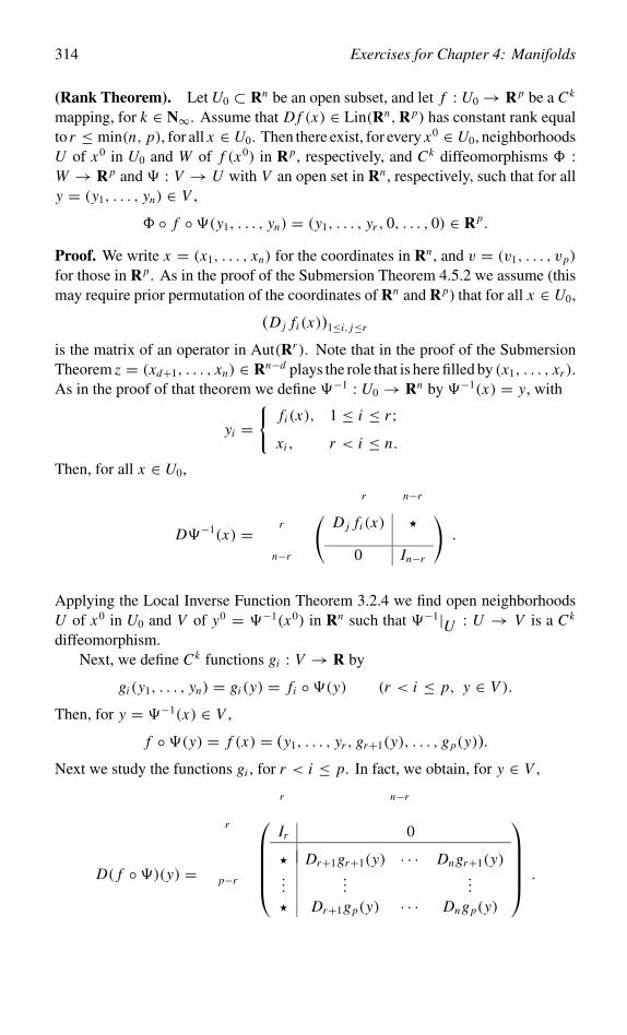
314 Exercises for Chapter 4: Manifolds
(Rank Theorem). Let U0 ⊂ Rn be an open subset, and let f : U0 → Rp be a Ck
mapping, for k ∈ N∞. Assume that D f (x) ∈ Lin(Rn,Rp) has constant rank equalto r ≤ min(n, p), for all x ∈ U0. Then there exist, for every x0 ∈ U0, neighborhoodsU of x0 in U0 and W of f (x0) in Rp, respectively, and Ck diffeomorphisms � :W → Rp and � : V → U with V an open set in Rn , respectively, such that for ally = (y1, . . . , yn) ∈ V ,
� ◦ f ◦�(y1, . . . , yn) = (y1, . . . , yr , 0, . . . , 0) ∈ Rp.
Proof. We write x = (x1, . . . , xn) for the coordinates in Rn , and v = (v1, . . . , vp)
for those in Rp. As in the proof of the Submersion Theorem 4.5.2 we assume (thismay require prior permutation of the coordinates of Rn and Rp) that for all x ∈ U0,
(D j fi (x))1≤i, j≤r
is the matrix of an operator in Aut(Rr ). Note that in the proof of the SubmersionTheorem z = (xd+1, . . . , xn) ∈ Rn−d plays the role that is here filled by (x1, . . . , xr ).As in the proof of that theorem we define �−1 : U0 → Rn by �−1(x) = y, with
yi ={
fi (x), 1 ≤ i ≤ r;xi , r < i ≤ n.
Then, for all x ∈ U0,
D�−1(x) =
r n−r
r
n−r
(D j fi (x) �
0 In−r
).
Applying the Local Inverse Function Theorem 3.2.4 we find open neighborhoodsU of x0 in U0 and V of y0 = �−1(x0) in Rn such that �−1|U : U → V is a Ck
diffeomorphism.Next, we define Ck functions gi : V → R by
gi (y1, . . . , yn) = gi (y) = fi ◦�(y) (r < i ≤ p, y ∈ V ).
Then, for y = �−1(x) ∈ V ,
f ◦�(y) = f (x) = (y1, . . . , yr , gr+1(y), . . . , gp(y)).
Next we study the functions gi , for r < i ≤ p. In fact, we obtain, for y ∈ V ,
D( f ◦�)(y) =
r n−r
r
p−r
Ir 0
� Dr+1gr+1(y) · · · Dngr+1(y)...
......
� Dr+1gp(y) · · · Dngp(y)
.
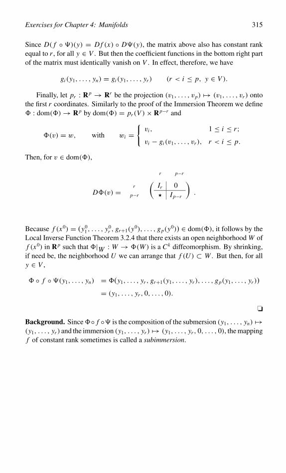
Exercises for Chapter 4: Manifolds 315
Since D( f ◦ �)(y) = D f (x) ◦ D�(y), the matrix above also has constant rankequal to r , for all y ∈ V . But then the coefficient functions in the bottom right partof the matrix must identically vanish on V . In effect, therefore, we have
gi (y1, . . . , yn) = gi (y1, . . . , yr ) (r < i ≤ p, y ∈ V ).
Finally, let pr : Rp → Rr be the projection (v1, . . . , vp) �→ (v1, . . . , vr ) ontothe first r coordinates. Similarly to the proof of the Immersion Theorem we define� : dom(�)→ Rp by dom(�) = pr (V )× Rp−r and
�(v) = w, with wi ={vi , 1 ≤ i ≤ r;vi − gi (v1, . . . , vr ), r < i ≤ p.
Then, for v ∈ dom(�),
D�(v) =
r p−r
r
p−r
(Ir 0� Ip−r
).
Because f (x0) = (y01 , . . . , y0
r , gr+1(y0), . . . , gp(y0)) ∈ dom(�), it follows by theLocal Inverse Function Theorem 3.2.4 that there exists an open neighborhood W off (x0) in Rp such that �|W : W → �(W ) is a Ck diffeomorphism. By shrinking,if need be, the neighborhood U we can arrange that f (U ) ⊂ W . But then, for ally ∈ V ,
� ◦ f ◦�(y1, . . . , yn) = �(y1, . . . , yr , gr+1(y1, . . . , yr ), . . . , gp(y1, . . . , yr ))
= (y1, . . . , yr , 0, . . . , 0).
❏
Background. Since�◦ f ◦� is the composition of the submersion (y1, . . . , yn) �→(y1, . . . , yr ) and the immersion (y1, . . . , yr ) �→ (y1, . . . , yr , 0, . . . , 0), the mappingf of constant rank sometimes is called a subimmersion.

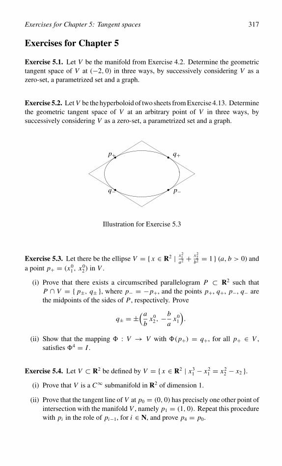
Exercises for Chapter 5: Tangent spaces 317
Exercises for Chapter 5
Exercise 5.1. Let V be the manifold from Exercise 4.2. Determine the geometrictangent space of V at (−2, 0) in three ways, by successively considering V as azero-set, a parametrized set and a graph.
Exercise 5.2. Let V be the hyperboloid of two sheets from Exercise 4.13. Determinethe geometric tangent space of V at an arbitrary point of V in three ways, bysuccessively considering V as a zero-set, a parametrized set and a graph.
p+
p−
q+
q−
Illustration for Exercise 5.3
Exercise 5.3. Let there be the ellipse V = { x ∈ R2 | x21
a2 + x22
b2 = 1 } (a, b > 0) anda point p+ = (x0
1 , x02) in V .
(i) Prove that there exists a circumscribed parallelogram P ⊂ R2 such thatP ∩ V = { p±, q± }, where p− = −p+, and the points p+, q+, p−, q− arethe midpoints of the sides of P , respectively. Prove
q± = ±(a
bx0
2 , −b
ax0
1
).
(ii) Show that the mapping � : V → V with �(p+) = q+, for all p+ ∈ V ,satisfies �4 = I .
Exercise 5.4. Let V ⊂ R2 be defined by V = { x ∈ R2 | x31 − x2
1 = x22 − x2 }.
(i) Prove that V is a C∞ submanifold in R2 of dimension 1.
(ii) Prove that the tangent line of V at p0 = (0, 0) has precisely one other point ofintersection with the manifold V , namely p1 = (1, 0). Repeat this procedurewith pi in the role of pi−1, for i ∈ N, and prove p4 = p0.
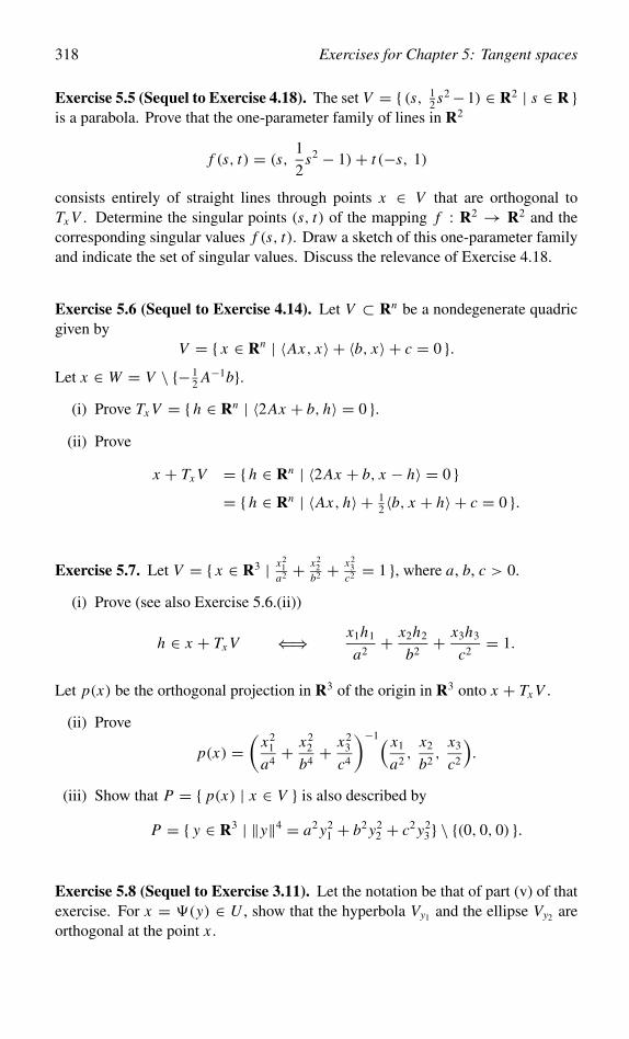
318 Exercises for Chapter 5: Tangent spaces
Exercise 5.5 (Sequel to Exercise 4.18). The set V = { (s, 12 s2−1) ∈ R2 | s ∈ R }
is a parabola. Prove that the one-parameter family of lines in R2
f (s, t) = (s,1
2s2 − 1)+ t (−s, 1)
consists entirely of straight lines through points x ∈ V that are orthogonal toTx V . Determine the singular points (s, t) of the mapping f : R2 → R2 and thecorresponding singular values f (s, t). Draw a sketch of this one-parameter familyand indicate the set of singular values. Discuss the relevance of Exercise 4.18.
Exercise 5.6 (Sequel to Exercise 4.14). Let V ⊂ Rn be a nondegenerate quadricgiven by
V = { x ∈ Rn | 〈Ax, x〉 + 〈b, x〉 + c = 0 }.Let x ∈ W = V \ {− 1
2 A−1b}.(i) Prove Tx V = { h ∈ Rn | 〈2Ax + b, h〉 = 0 }.
(ii) Prove
x + Tx V = { h ∈ Rn | 〈2Ax + b, x − h〉 = 0 }= { h ∈ Rn | 〈Ax, h〉 + 1
2 〈b, x + h〉 + c = 0 }.
Exercise 5.7. Let V = { x ∈ R3 | x21
a2 + x22
b2 + x23
c2 = 1 }, where a, b, c > 0.
(i) Prove (see also Exercise 5.6.(ii))
h ∈ x + Tx V ⇐⇒ x1h1
a2+ x2h2
b2+ x3h3
c2= 1.
Let p(x) be the orthogonal projection in R3 of the origin in R3 onto x + Tx V .
(ii) Prove
p(x) =(
x21
a4+ x2
2
b4+ x2
3
c4
)−1( x1
a2,
x2
b2,
x3
c2
).
(iii) Show that P = { p(x) | x ∈ V } is also described by
P = { y ∈ R3 | ‖y‖4 = a2 y21 + b2 y2
2 + c2 y23} \ {(0, 0, 0) }.
Exercise 5.8 (Sequel to Exercise 3.11). Let the notation be that of part (v) of thatexercise. For x = �(y) ∈ U , show that the hyperbola Vy1 and the ellipse Vy2 areorthogonal at the point x .
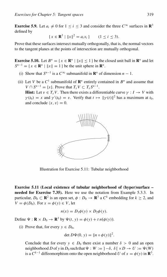
Exercises for Chapter 5: Tangent spaces 319
Exercise 5.9. Let ai = 0 for 1 ≤ i ≤ 3 and consider the three C∞ surfaces in R3
defined by{ x ∈ R3 | ‖x‖2 = ai xi } (1 ≤ i ≤ 3).
Prove that these surfaces intersect mutually orthogonally, that is, the normal vectorsto the tangent planes at the points of intersection are mutually orthogonal.
Exercise 5.10. Let Bn = { x ∈ Rn | ‖x‖ ≤ 1 } be the closed unit ball in Rn and letSn−1 = { x ∈ Rn | ‖x‖ = 1 } be the unit sphere in Rn .
(i) Show that Sn−1 is a C∞ submanifold in Rn of dimension n − 1.
(ii) Let V be a C1 submanifold of Rn entirely contained in Bn and assume thatV ∩ Sn−1 = {x}. Prove that Tx V ⊂ Tx Sn−1.Hint: Let v ∈ Tx V . Then there exists a differentiable curve γ : I → V withγ (t0) = x and γ ′(t0) = v. Verify that t �→ ‖γ (t)‖2 has a maximum at t0,and conclude 〈x, v〉 = 0.
Illustration for Exercise 5.11: Tubular neighborhood
Exercise 5.11 (Local existence of tubular neighborhood of (hyper)surface –needed for Exercise 7.35). Here we use the notation from Example 5.3.3. Inparticular, D0 ⊂ R2 is an open set, φ : D0 → R3 a Ck embedding for k ≥ 2, andV = φ(D0). For x = φ(y) ∈ V , let
n(x) = D1φ(y)× D2φ(y).
Define � : R × D0 → R3 by �(t, y) = φ(y)+ t n(φ(y)).
(i) Prove that, for every y ∈ D0,
det D�(0, y) = ‖n ◦ φ(y)‖2.
Conclude that for every y ∈ D0 there exist a number δ > 0 and an openneighborhood D of y in D0 such that� : W := ]−δ, δ [×D → U := �(W )
is a Ck−1 diffeomorphism onto the open neighborhood U of x = φ(y) in R3.
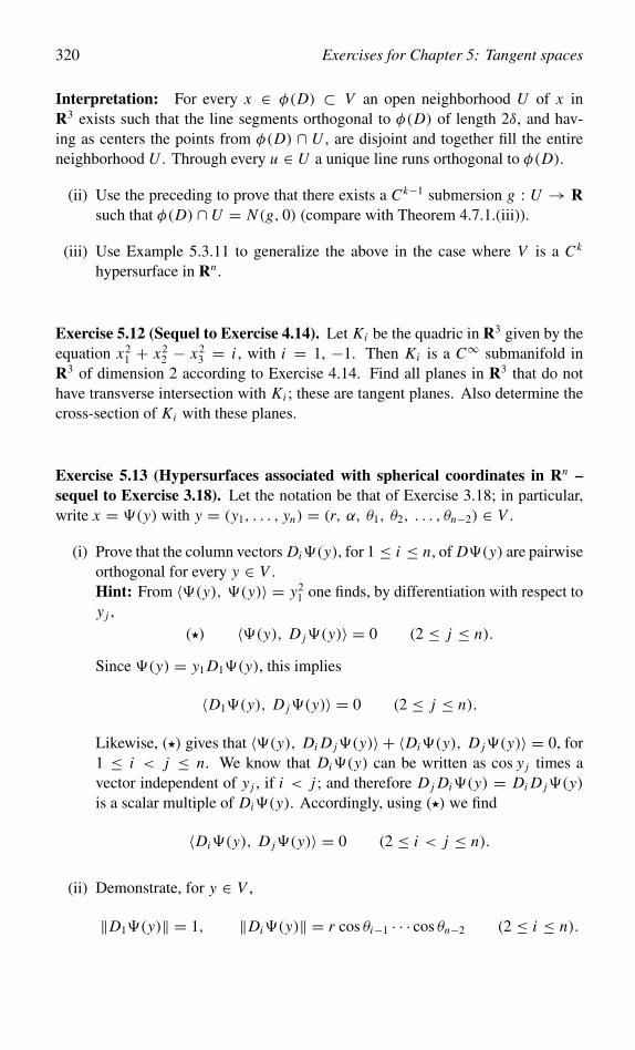
320 Exercises for Chapter 5: Tangent spaces
Interpretation: For every x ∈ φ(D) ⊂ V an open neighborhood U of x inR3 exists such that the line segments orthogonal to φ(D) of length 2δ, and hav-ing as centers the points from φ(D) ∩ U , are disjoint and together fill the entireneighborhood U . Through every u ∈ U a unique line runs orthogonal to φ(D).
(ii) Use the preceding to prove that there exists a Ck−1 submersion g : U → Rsuch that φ(D) ∩U = N (g, 0) (compare with Theorem 4.7.1.(iii)).
(iii) Use Example 5.3.11 to generalize the above in the case where V is a Ck
hypersurface in Rn .
Exercise 5.12 (Sequel to Exercise 4.14). Let Ki be the quadric in R3 given by theequation x2
1 + x22 − x2
3 = i , with i = 1, −1. Then Ki is a C∞ submanifold inR3 of dimension 2 according to Exercise 4.14. Find all planes in R3 that do nothave transverse intersection with Ki ; these are tangent planes. Also determine thecross-section of Ki with these planes.
Exercise 5.13 (Hypersurfaces associated with spherical coordinates in Rn –sequel to Exercise 3.18). Let the notation be that of Exercise 3.18; in particular,write x = �(y) with y = (y1, . . . , yn) = (r, α, θ1, θ2, . . . , θn−2) ∈ V .
(i) Prove that the column vectors Di�(y), for 1 ≤ i ≤ n, of D�(y) are pairwiseorthogonal for every y ∈ V .Hint: From 〈�(y), �(y)〉 = y2
1 one finds, by differentiation with respect toy j ,
(�) 〈�(y), D j�(y)〉 = 0 (2 ≤ j ≤ n).
Since �(y) = y1 D1�(y), this implies
〈D1�(y), D j�(y)〉 = 0 (2 ≤ j ≤ n).
Likewise, (�) gives that 〈�(y), Di D j�(y)〉 + 〈Di�(y), D j�(y)〉 = 0, for1 ≤ i < j ≤ n. We know that Di�(y) can be written as cos y j times avector independent of y j , if i < j ; and therefore D j Di�(y) = Di D j�(y)is a scalar multiple of Di�(y). Accordingly, using (�) we find
〈Di�(y), D j�(y)〉 = 0 (2 ≤ i < j ≤ n).
(ii) Demonstrate, for y ∈ V ,
‖D1�(y)‖ = 1, ‖Di�(y)‖ = r cos θi−1 · · · cos θn−2 (2 ≤ i ≤ n).
Exercises for Chapter 5: Tangent spaces 321
Hint: Check
(��) � j (y) = � j (y1, y j , . . . , yn) (1 ≤ j ≤ n),
(� � �)∑
1≤ j≤i
� j (y)2 = y2
1 cos2 yi+1 · · · cos2 yn (1 ≤ i ≤ n).
Let 2 ≤ i ≤ n. Then (��) implies that
Di�(y)t = (Di�1(y), . . . , Di�i (y), 0, . . . , 0),
and (���) yields�1 Di�1+· · ·+�i Di�i = 0. Show thatD2i � j = −� j , for
1 ≤ j ≤ i , and thereby prove (Di�1)2+· · ·+(Di�i )
2−�21−· · ·−�2
i = 0.
(iii) Using the preceding parts, prove the formula from Exercise 3.18.(iii)
det D�(y) = rn−1 cos θ1 cos2 θ2 · · · cosn−2 θn−2.
(iv) Given y0 ∈ V , the hypersurfaces {�(y) ∈ Rn | y ∈ V, y j = y0j }, for
1 ≤ j ≤ n, all go through �(y0). Prove by means of part (i) that thesehypersurfaces in Rn are mutually orthogonal at the point �(y0).
Exercise 5.14. Let V be a Ck submanifold in Rn of dimension d, and let x0 ∈ V .Let ψ : Rn−d → Rn be a Ck mapping with ψ(0) = 0. Define f : V ×Rn−d → Rn
by f (x, y) = x + ψ(y). Then prove the equivalence of the following assertions.
(i) There exist open neighborhoods U of x0 in Rn and W of 0 in Rn−d such thatf |(V∩U )×W is a Ck diffeomorphism onto a neighborhood of x0 in Rn .
(ii) im Dψ(0) ∩ Tx0 V = {0}.
Exercise 5.15. Suppose that V is a Ck submanifold in Rn of dimension d, considerA ∈ Lin(Rn,Rd) and let x ∈ V . Prove that the following assertions are equivalent.
(i) There exists an open neighborhood U of x in Rn such that A|V∩U is a Ck
diffeomorphism from V ∩U onto an open neighborhood of Ax in Rd .
(ii) ker A ∩ Tx V = {0}.Prove that assertion (ii) implies that A is surjective.
Exercise 5.16 (Implicit Function Theorem in geometric form). We consider theImplicit Function Theorem 3.5.1 and some of its relations to manifolds and tangentspaces. Let the notation and the assumptions be as in the theorem. Furthermore,we write v0 = (x0, y0) and V0 = { (x, y) ∈ U × V | f (x; y) = 0 }
322 Exercises for Chapter 5: Tangent spaces
(i) Show that V0 is a submanifold in Rn × Rp of dimension p. Prove that
Tv0 V0 = { (ξ, η) ∈ Rn × Rp | Dx f (v0)ξ + Dy f (v0)η = 0 }= { (ξ, η) ∈ Rn × Rp | ξ = Dψ(y0)η }.
Denote byπ : Rn×Rp → Rp the projection along Rn onto Rp, satisfyingπ(ξ, η) =η.
(ii) Show that π |Tv0 V0∈ Lin(Tv0 V0,Rp) is a bijection. Conversely, if this map-
ping is given to be a bijection, prove that the condition Dx f (v0) ∈ Aut(Rn)
from the Implicit Function Theorem is satisfied.
Exercise 5.17 (Tangent bundle of submanifold). Let k ∈ N, let V be a Ck sub-manifold in Rn of dimension d, let x ∈ V and v ∈ Tx V . Then (x, v) ∈ R2n is saidto be a (geometric) tangent vector of V . Define T V , the tangent bundle of V , asthe subset of R2n consisting of all (geometric) tangent vectors of V .
(i) Use the local description of V∩U = N (g, 0) according to Theorem 4.7.1.(iii)and consider the Ck−1 mapping
G : U × Rn → Rn−d × Rn−d with G(x, v) =( g(x)
Dg(x)v
).
Verify that (x, v) ∈ U × Rn belongs to T V if and only if G(x, v) = 0.
(ii) Prove that DG(x, v) ∈ Lin(R2n,R2n−2d) is given by
DG(x, v)(ξ, η) =( Dg(x)ξ
D2g(x)(ξ, v)+ Dg(x)η
)((ξ, η) ∈ R2n).
Deduce that G is a Ck−1 submersion and apply the Submersion Theorem 4.5.2to show that T V is a Ck−1 submanifold in R2n of dimension 2d.
(iii) Denote by π : T V → V the projection of the bundle onto the base space Vgiven by π(x, v) = x . Show that π−1({x}) = Tx V , for all x ∈ V , that is, thetangent spaces are the fibres of the projection.
Background. One may think of the tangent bundle of V as the disjoint unionof the tangent spaces at all points of V . The reason for taking the disjoint unionof the tangent spaces is the following: although all the geometric tangent spacesx+Tx V are affinely isomorphic with Rd , geometrically they might differ from eachother although they might intersect, and we do not wish to water this fact down byincluding into the union just one point from among the points lying in each of thesedifferent tangent spaces.
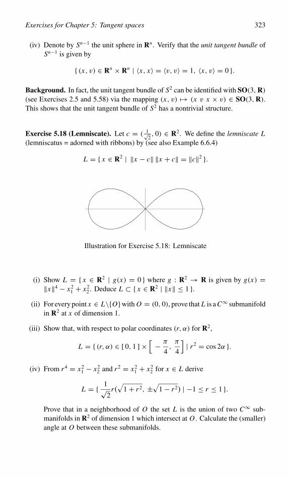
Exercises for Chapter 5: Tangent spaces 323
(iv) Denote by Sn−1 the unit sphere in Rn . Verify that the unit tangent bundle ofSn−1 is given by
{ (x, v) ∈ Rn × Rn | 〈x, x〉 = 〈v, v〉 = 1, 〈x, v〉 = 0 }.
Background. In fact, the unit tangent bundle of S2 can be identified with SO(3,R)(see Exercises 2.5 and 5.58) via the mapping (x, v) �→ (x v x × v) ∈ SO(3,R).This shows that the unit tangent bundle of S2 has a nontrivial structure.
Exercise 5.18 (Lemniscate). Let c = ( 1√2, 0) ∈ R2. We define the lemniscate L
(lemniscatus = adorned with ribbons) by (see also Example 6.6.4)
L = { x ∈ R2 | ‖x − c‖ ‖x + c‖ = ‖c‖2 }.
Illustration for Exercise 5.18: Lemniscate
(i) Show L = { x ∈ R2 | g(x) = 0 } where g : R2 → R is given by g(x) =‖x‖4 − x2
1 + x22 . Deduce L ⊂ { x ∈ R2 | ‖x‖ ≤ 1 }.
(ii) For every point x ∈ L\{O}with O = (0, 0), prove that L is a C∞ submanifoldin R2 at x of dimension 1.
(iii) Show that, with respect to polar coordinates (r, α) for R2,
L = { (r, α) ∈ [ 0, 1 ] ×[− π
4,π
4
]| r2 = cos 2α }.
(iv) From r4 = x21 − x2
2 and r2 = x21 + x2
2 for x ∈ L derive
L = { 1√2
r(√
1+ r2, ±√
1− r2) | −1 ≤ r ≤ 1 }.
Prove that in a neighborhood of O the set L is the union of two C∞ sub-manifolds in R2 of dimension 1 which intersect at O . Calculate the (smaller)angle at O between these submanifolds.
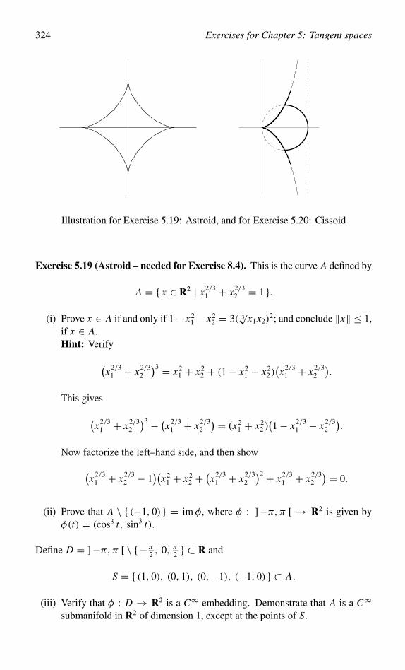
324 Exercises for Chapter 5: Tangent spaces
Illustration for Exercise 5.19: Astroid, and for Exercise 5.20: Cissoid
Exercise 5.19 (Astroid – needed for Exercise 8.4). This is the curve A defined by
A = { x ∈ R2 | x2/31 + x2/3
2 = 1 }.
(i) Prove x ∈ A if and only if 1− x21 − x2
2 = 3( 3√
x1x2)2; and conclude ‖x‖ ≤ 1,
if x ∈ A.Hint: Verify
(x2/3
1 + x2/32
)3 = x21 + x2
2 + (1− x21 − x2
2)(x2/3
1 + x2/32
).
This gives
(x2/3
1 + x2/32
)3 − (x2/3
1 + x2/32
) = (x21 + x2
2 )(1− x2/3
1 − x2/32
).
Now factorize the left–hand side, and then show(x2/3
1 + x2/32 − 1
)(x2
1 + x22 +
(x2/3
1 + x2/32
)2 + x2/31 + x2/3
2
) = 0.
(ii) Prove that A \ { (−1, 0) } = im φ, where φ : ]−π, π [ → R2 is given byφ(t) = (cos3 t, sin3 t).
Define D = ]−π, π [ \ {−π2 , 0, π2 } ⊂ R and
S = { (1, 0), (0, 1), (0,−1), (−1, 0) } ⊂ A.
(iii) Verify that φ : D → R2 is a C∞ embedding. Demonstrate that A is a C∞submanifold in R2 of dimension 1, except at the points of S.
Exercises for Chapter 5: Tangent spaces 325
(iv) Verify that the slope of the tangent line of A at φ(t) equals − tan t , if t =−π
2 ,π2 . Now prove by Taylor expansion of φ(t) for t → 0 and by symmetry
arguments that A has an ordinary cusp at the points of S. Conclude that A isnot a C1 submanifold in R2 of dimension 1 at the points of S.
Exercise 5.20 (Diocles’ cissoid). (� κισσ�ς = ivy.) Let 0 ≤ y <√
2. Then thevertical line in R2 through the point (2− y2, 0) has a unique point of intersection,say χ(y) ∈ R2, with the circular arc { x ∈ R2 | ‖x − (1, 0)‖ = 1, x2 ≥ 0 }; andχ(y) = (0, 0). The straight line through (0, 0) and χ(y) intersects the vertical linethrough (y2, 0) at a unique point, say φ(y) ∈ R2.
(i) Verify that
φ(y) =(
y2,y3√
2− y2
)(0 ≤ y <
√2).
(ii) Show that the mapping φ : ] 0,√
2[→ R2 given in (i) is a C∞ embedding.
Diocles’ cissoid is the set V ⊂ R2 defined by
V ={(
y2,y3√
2− y2
)∈ R2
∣∣∣∣ −√2 < y <√
2
}.
(iii) Show that V \ {(0, 0)} is a C∞ submanifold in R2 of dimension 1.
(iv) Prove V = g−1({0}), with g(x) = x31 + (x1 − 2)x2
2 .
(v) Show that g : R2 → R is surjective, and that, for every c ∈ R \ {0}, the levelset g−1({c}) is a C∞ submanifold in R2 of dimension 1.
(vi) Prove by Taylor expansion that V has an ordinary cusp at the point (0, 0),and deduce that at the point (0, 0) the set V is not a C1 submanifold in R2 ofdimension 1.
Exercise 5.21 (Conchoid and trisection of angle). ( κ�γχη= shell.) A Nicomedesconchoid is a curve K in R2 defined as follows. Let O = (0, 0) ∈ R2. Let d > 0be arbitrary. Choose a point A on the line x1 = 1. Then the line through A and Ocontains two points, say PA and P ′A, whose distance to A equals d. Define K = Kd
as the collection of these points PA and P ′A, for all possible A. Define the C∞mapping gd : R2 → R by
gd(x) = x41 + x2
1 x22 − 2x3
1 − 2x1x22 + (1− d2)x2
1 + x22 .
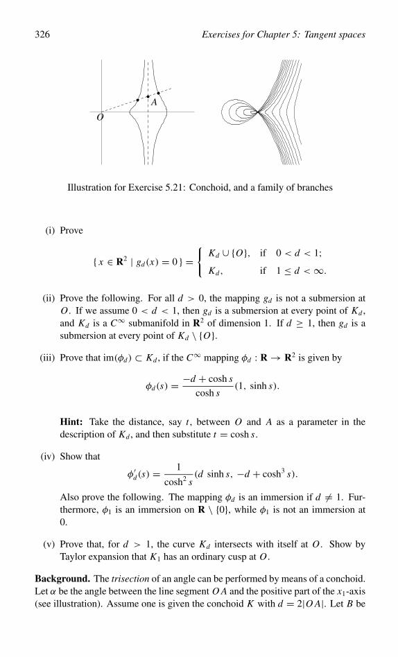
326 Exercises for Chapter 5: Tangent spaces
O
A
Illustration for Exercise 5.21: Conchoid, and a family of branches
(i) Prove
{ x ∈ R2 | gd(x) = 0 } ={
Kd ∪ {O}, if 0 < d < 1;Kd, if 1 ≤ d <∞.
(ii) Prove the following. For all d > 0, the mapping gd is not a submersion atO . If we assume 0 < d < 1, then gd is a submersion at every point of Kd ,and Kd is a C∞ submanifold in R2 of dimension 1. If d ≥ 1, then gd is asubmersion at every point of Kd \ {O}.
(iii) Prove that im(φd) ⊂ Kd , if the C∞ mapping φd : R → R2 is given by
φd(s) = −d + cosh s
cosh s(1, sinh s).
Hint: Take the distance, say t , between O and A as a parameter in thedescription of Kd , and then substitute t = cosh s.
(iv) Show that
φ′d(s) =1
cosh2 s(d sinh s, −d + cosh3 s).
Also prove the following. The mapping φd is an immersion if d = 1. Fur-thermore, φ1 is an immersion on R \ {0}, while φ1 is not an immersion at0.
(v) Prove that, for d > 1, the curve Kd intersects with itself at O . Show byTaylor expansion that K1 has an ordinary cusp at O .
Background. The trisection of an angle can be performed by means of a conchoid.Let α be the angle between the line segment O A and the positive part of the x1-axis(see illustration). Assume one is given the conchoid K with d = 2|O A|. Let B be
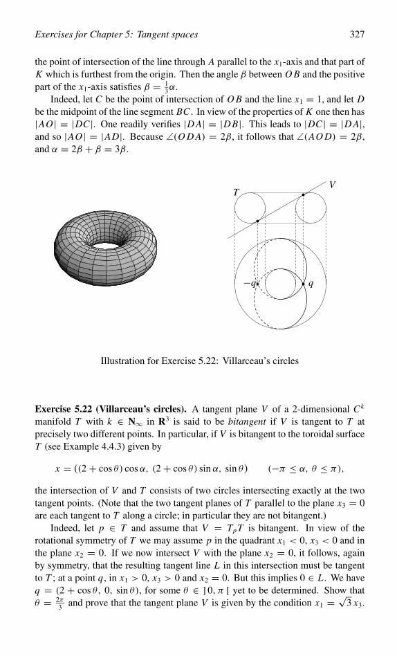
Exercises for Chapter 5: Tangent spaces 327
the point of intersection of the line through A parallel to the x1-axis and that part ofK which is furthest from the origin. Then the angle β between O B and the positivepart of the x1-axis satisfies β = 1
3α.Indeed, let C be the point of intersection of O B and the line x1 = 1, and let D
be the midpoint of the line segment BC . In view of the properties of K one then has|AO| = |DC |. One readily verifies |D A| = |DB|. This leads to |DC | = |D A|,and so |AO| = |AD|. Because ∠(O D A) = 2β, it follows that ∠(AO D) = 2β,and α = 2β + β = 3β.
TV
q−q
Illustration for Exercise 5.22: Villarceau’s circles
Exercise 5.22 (Villarceau’s circles). A tangent plane V of a 2-dimensional Ck
manifold T with k ∈ N∞ in R3 is said to be bitangent if V is tangent to T atprecisely two different points. In particular, if V is bitangent to the toroidal surfaceT (see Example 4.4.3) given by
x = ((2+ cos θ) cosα, (2+ cos θ) sin α, sin θ) (−π ≤ α, θ ≤ π),
the intersection of V and T consists of two circles intersecting exactly at the twotangent points. (Note that the two tangent planes of T parallel to the plane x3 = 0are each tangent to T along a circle; in particular they are not bitangent.)
Indeed, let p ∈ T and assume that V = TpT is bitangent. In view of therotational symmetry of T we may assume p in the quadrant x1 < 0, x3 < 0 and inthe plane x2 = 0. If we now intersect V with the plane x2 = 0, it follows, againby symmetry, that the resulting tangent line L in this intersection must be tangentto T ; at a point q, in x1 > 0, x3 > 0 and x2 = 0. But this implies 0 ∈ L . We haveq = (2 + cos θ, 0, sin θ), for some θ ∈ ] 0, π [ yet to be determined. Show thatθ = 2π
3 and prove that the tangent plane V is given by the condition x1 =√
3 x3.
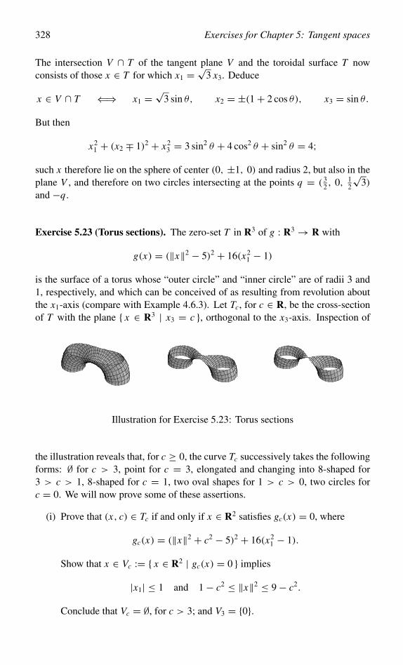
328 Exercises for Chapter 5: Tangent spaces
The intersection V ∩ T of the tangent plane V and the toroidal surface T nowconsists of those x ∈ T for which x1 =
√3 x3. Deduce
x ∈ V ∩ T ⇐⇒ x1 =√
3 sin θ, x2 = ±(1+ 2 cos θ), x3 = sin θ.
But then
x21 + (x2 ∓ 1)2 + x2
3 = 3 sin2 θ + 4 cos2 θ + sin2 θ = 4;
such x therefore lie on the sphere of center (0, ±1, 0) and radius 2, but also in theplane V , and therefore on two circles intersecting at the points q = ( 3
2 , 0, 12
√3)
and −q.
Exercise 5.23 (Torus sections). The zero-set T in R3 of g : R3 → R with
g(x) = (‖x‖2 − 5)2 + 16(x21 − 1)
is the surface of a torus whose “outer circle” and “inner circle” are of radii 3 and1, respectively, and which can be conceived of as resulting from revolution aboutthe x1-axis (compare with Example 4.6.3). Let Tc, for c ∈ R, be the cross-sectionof T with the plane { x ∈ R3 | x3 = c }, orthogonal to the x3-axis. Inspection of
Illustration for Exercise 5.23: Torus sections
the illustration reveals that, for c ≥ 0, the curve Tc successively takes the followingforms: ∅ for c > 3, point for c = 3, elongated and changing into 8-shaped for3 > c > 1, 8-shaped for c = 1, two oval shapes for 1 > c > 0, two circles forc = 0. We will now prove some of these assertions.
(i) Prove that (x, c) ∈ Tc if and only if x ∈ R2 satisfies gc(x) = 0, where
gc(x) = (‖x‖2 + c2 − 5)2 + 16(x21 − 1).
Show that x ∈ Vc := { x ∈ R2 | gc(x) = 0 } implies
|x1| ≤ 1 and 1− c2 ≤ ‖x‖2 ≤ 9− c2.
Conclude that Vc = ∅, for c > 3; and V3 = {0}.
Exercises for Chapter 5: Tangent spaces 329
(ii) Verify that 0 ∈ Vc with c ≥ 0 implies c = 3 or c = 1; prove that in thesecases gc is nonsubmersive at 0 ∈ R2. Verify that gc is submersive at everypoint of Vc \ {0}, for all c ≥ 0. Show that Vc is a C∞ submanifold in R2 ofdimension 1, for every c with 3 > c > 1 or 1 > c ≥ 0.
(iii) Define
φ± :] −√2,
√2[→ R2 by φ±(t) = t(
√2− t2, ±
√2+ t2).
By intersecting V1 with circles around 0 of radius 2t , demonstrate that V1 =im(φ+) ∪ im(φ−). Conclude that V1 intersects with itself at 0 at an angle ofπ2 radians.
(iv) Draw a single sketch showing, in a neighborhood of 0 ∈ R2, the three mani-folds Vc, for c slightly larger than 1, for c = 1, and for c slightly smaller than1. Prove that, for c near 1, the Vc qualitatively have the properties sketched.Hint: With t in a suitable neighborhood of 0, substitute ‖x‖2 = 4t2
√1− d,
where 5− c2 = 4√
1− d. One therefore has d in a neighborhood of 0. Onefinds
x21 = d + 2(1− d)t2 − (1− d)t4,
x22 = −d + 2(2
√1− d − 1+ d)t2 + (1− d)t4.
Now determine, in particular, for which c one has x21 � x2
2 for x ∈ Vc, andestablish whether the Vc go through 0.
Exercise 5.24 (Conic section in polar coordinates – needed for Exercises 5.53and 6.28). Let t �→ x(t) be a differentiable curve in R2 and let f± ∈ R2 be twodistinct fixed points, called the foci. Suppose the angle between x(t)− f− and−x ′(t)equals the angle between x(t) − f+ and x ′(t), for all t ∈ R (angle of incidenceequals angle of reflection).
(i) Prove
∑±
〈 x(t)− f±, x ′(t)〉‖x(t)− f±‖ = 0; hence
(∑±‖x(t)− f±‖
)′= 0,
on account of Example 2.4.8. Deduce∑± ‖x(t) − f±‖ = 2a, for some
a ≥ 12‖ f+ − f−‖ > 0 and all t ∈ R.
(ii) By a translation, if necessary, we may assume f− = 0. For a > 0 andf+ ∈ R2 with ‖ f+‖ = 2a, we define the two sets C+ and C− by C± = { x ∈R2 | ±‖x − f+‖ = 2a − ‖x‖ }. Then
C := { x ∈ R2 | ‖x‖ = 〈x, ε〉 + d } ={
C+, d > 0;C−, d < 0.
330 Exercises for Chapter 5: Tangent spaces
Here we introduced the eccentricity vector ε = 12a f+ ∈ R2 and d =
4a2−‖ f+‖2
4a ∈ R. Next, define the numbers e ≥ 0, the eccentricity of C ,and c > 0 and b ≥ 0 by
‖ε‖ = e = c
a=√
a2 ∓ b2
aas e ≶ 1.
Deduce that ‖ f+‖ = 2c, in other words, the distance between the foci equals2c, and that d = a(1− e2) = ± b2
a as e ≶ 1. Conversely, for e = 1,
a = d
1− e2, b = ±d√±(1− e2)
as e ≶ 1.
Consider x ∈ R2 perpendicular to f+ of length d. Prove that x ∈ C if d > 0,and f+ + x ∈ C if d < 0. The chord of C perpendicular to ε of length 2d iscalled the latus rectum of C .
(iii) Use part (ii) to show that the substitution of variables x = y + aε turns theequation ‖x‖2 = (〈x, ε〉 + d)2 into
‖y‖2 − 〈y, ε〉2 = ±b2, that isy2
1
a2± y2
2
b2= 1, as e ≶ 1.
In the latter equation ε is assumed to be along the y1-axis; this may requirea rotation about the origin. Furthermore, it is the equation of a conic sectionwith ε along the line connecting the foci. Deduce that C equals the ellipseC+ with semimajor axis a and semiminor axis b if 0 < e < 1, a parabola ife = 1, and the branch C− nearest to f+ of the hyperbola with transverse axisa and conjugate axis b if e > 1. (For the other branch, which is nearest to 0,of the hyperbola, consider −d > 0; this corresponds to the choice of a < 0,and an element x in that branch satisfies ‖x − f+‖ − ‖x‖ = 2a.)
(iv) Finally, introduce polar coordinates (r, α)by r = ‖x‖ and cosα = − 〈x,ε〉‖x‖ ‖ε‖ =
−〈x,ε〉re (this choice makes the periapse, that is, the point of C nearest to the
origin correspond with α = 0). Show that the equation for C takes the formr = d
1+e cosα , compare with Exercise 4.2.
Exercise 5.25 (Heron’s formula and sine and cosine rule – needed for Exer-cise 5.39). Let � ⊂ R2 be a triangle of area O whose sides have lengths Ai , for1 ≤ i ≤ 3, respectively. We then write 2S =∑
1≤i≤3 Ai for the perimeter of �.
(i) Prove the following, known as Heron’s formula:
O2 = S(S − A1)(S − A2)(S − A3).
Hint: We may assume the vertices of � to be given by the vectors a3 =
Exercises for Chapter 5: Tangent spaces 331
0, a1 and a2 ∈ R2. Then 2 O = det(a1 a2) (a triangle is one half of aparallelogram), and so
4 O2 =∣∣∣∣∣ ‖a1‖2 〈 a2, a1 〉〈 a1, a2 〉 ‖a2‖2
∣∣∣∣∣= (‖a1‖‖a2‖ + 〈 a1, a2 〉)(‖a1‖‖a2‖ − 〈 a1, a2 〉)
= 1
4((‖a1‖ + ‖a2‖)2 − ‖a1 − a2‖2)(‖a1 − a2‖2 − (‖a1‖ − ‖a2‖)2).
Now write ‖a1‖ = A2, ‖a2‖ = A1 and ‖a1 − a2‖ = A3.
(ii) Note that the first identity above is equivalent to 2 O = A1 A2 sin ∠(a1, a2),that is, O is half the height times the length of the base. Denote by αi theangle of � opposite Ai , for 1 ≤ i ≤ 3. Deduce the following sine rule, andthe cosine rule, respectively, for � and 1 ≤ i ≤ 3:
sin αi
Ai= 2O∏
1≤i≤3 Ai, A2
i = A2i+1 + A2
i+2 − 2Ai+1 Ai+2 cosαi .
In the latter formula the indices 1 ≤ i ≤ 3 are taken modulo 3.
Exercise 5.26 (Cauchy–Schwarz inequality in Rn , Grassmann’s, Jacobi’s andLagrange’s identities in R3 – needed for Exercises 5.27, 5.58, 5.59, 5.65, 5.66and 5.67).
(i) Show, for v and w ∈ Rn (compare with the Remark on linear algebra inExample 5.3.11 and see Exercise 7.1.(ii) for another proof),
〈v,w〉2 +∑
1≤i< j≤n
(viw j − v jwi )2 = ‖v‖2 ‖w‖2.
Derive from this the Cauchy–Schwarz inequality |〈v,w〉| ≤ ‖v‖ ‖w‖, for vand w ∈ Rn .
Assume v1, v2, v3 and v4 arbitrary vectors in R3.
(ii) Prove the following, known as Grassmann’s identity, by writing out the com-ponents on both sides:
v1 × (v2 × v3) = 〈 v3, v1 〉 v2 − 〈 v1, v2 〉 v3.
Background. Here is a rule to remember this formula. Note v1 × (v2 × v3) isperpendicular to v2 × v3; hence, it is a linear combination λ v2 + µv3 of v2 andv3. Because it is perpendicular to v1 too, we have λ〈v1, v2〉 + µ〈v3, v1〉 = 0; and,indeed, this is satisfied by λ = 〈v3, v1〉 andµ = −〈v1, v2〉. It turns out to be tediousto convert this argument into a rigorous proof.
332 Exercises for Chapter 5: Tangent spaces
Instead we give another proof of Grassmann’s identity. Let (e1, e2, e3) denotethe standard basis in R3. Given any two different indices i and j , let k denote thethird index different from i and j . Then ei × e j = det(ei e j ek) ek . We obtain, forany two distinct indices i and j ,
〈ei , e j×(v2×v3)〉 = 〈ei×e j , v2×v3〉 = det(ei e j ek)〈ek, v2×v3〉 = v2i v3 j−v2 j v3i .
Obviously this is also valid if i = j . Therefore i can be chosen arbitrarily, and thuswe find, for all j ,
e j × (v2 × v3) = v3 j v2 − v2 j v3 = 〈v3, e j 〉v2 − 〈e j , v2〉v3.
Grassmann’s identity now follows by linearity.
(iii) Prove the following, known as Jacobi’s identity:
v1 × (v2 × v3)+ v2 × (v3 × v1)+ v3 × (v1 × v2) = 0.
For an alternative proof of Jacobi’s identity, show that
(v1, v2, v3, v4) �→ 〈 v4×v1, v2×v3 〉+〈 v4×v2, v3×v1 〉+〈 v4×v3, v1×v2 〉is an antisymmetric 4-linear form on R3, which implies that it is identically0.
Background. An algebra for which multiplication is anticommutative and whichsatisfies Jacobi’s identity is known as a Lie algebra. Obviously R3, regarded as avector space over R, and further endowed with the cross multiplication of vectors,is a Lie algebra.
(iv) Demonstrate
(v1 × v2)× (v3 × v4) = det(v4 v1 v2) v3 − det(v1 v2 v3) v4,
and also the following, known as Lagrange’s identity:
〈v1×v2, v3×v4〉 = 〈v1, v3〉 〈v2, v4〉−〈v1, v4〉 〈v2, v3〉 =∣∣∣∣ 〈v1, v3〉 〈v1, v4〉〈v2, v3〉 〈v2, v4〉
∣∣∣∣.Verify that the identity 〈v1, v2〉2+‖v1× v2‖2 = ‖v1‖2 ‖v2‖2 is a special caseof Lagrange’s identity.
(v) Alternatively, verify that Lagrange’s identity follows from Formula 5.3 byuse of the polarization identity from Lemma 1.1.5.(iii). Next use
〈v1 × v2, v3 × v4〉 = 〈v1, v2 × (v3 × v4)〉to obtain Grassmann’s identity in a way which does not depend on writingout the components.
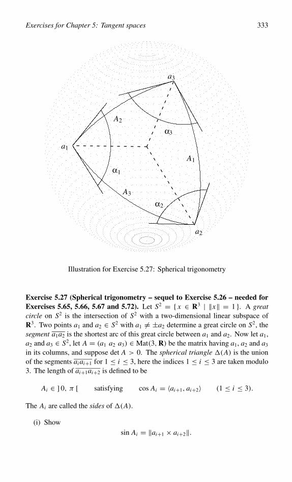
Exercises for Chapter 5: Tangent spaces 333
a1
a2
a3
A1
A3
A2
1
2
3
α
α
α
Illustration for Exercise 5.27: Spherical trigonometry
Exercise 5.27 (Spherical trigonometry – sequel to Exercise 5.26 – needed forExercises 5.65, 5.66, 5.67 and 5.72). Let S2 = { x ∈ R3 | ‖x‖ = 1 }. A greatcircle on S2 is the intersection of S2 with a two-dimensional linear subspace ofR3. Two points a1 and a2 ∈ S2 with a1 = ±a2 determine a great circle on S2, thesegment a1a2 is the shortest arc of this great circle between a1 and a2. Now let a1,a2 and a3 ∈ S2, let A = (a1 a2 a3) ∈ Mat(3,R) be the matrix having a1, a2 and a3
in its columns, and suppose det A > 0. The spherical triangle �(A) is the unionof the segments ai ai+1 for 1 ≤ i ≤ 3, here the indices 1 ≤ i ≤ 3 are taken modulo3. The length of ai+1ai+2 is defined to be
Ai ∈ ] 0, π [ satisfying cos Ai = 〈ai+1, ai+2〉 (1 ≤ i ≤ 3).
The Ai are called the sides of �(A).
(i) Showsin Ai = ‖ai+1 × ai+2‖.
334 Exercises for Chapter 5: Tangent spaces
The angles of �(A) are defined to be the angles αi ∈ ] 0, π [ between the tangentvectors at ai to ai ai+1, and ai ai+2, respectively.
(ii) Apply Lagrange’s identity in Exercise 5.26.(iv) to show
cosαi = 〈 ai × ai+1, ai × ai+2 〉‖ai × ai+1‖ ‖ai × ai+2‖ =
〈ai+1, ai+2〉 − 〈ai , ai+1〉 〈ai , ai+2〉‖ai × ai+1‖ ‖ai × ai+2‖ .
(iii) Use the definition of cos Ai and parts (i) and (ii) to deduce the spherical ruleof cosines for �(A)
cos Ai = cos Ai+1 cos Ai+2 + sin Ai+1 sin Ai+2 cosαi .
Replace the Ai by δAi with δ > 0, and show that Taylor expansion followedby taking the limit of the cosine rule for δ ↓ 0 leads to the cosine rule for aplanar triangle as in Exercise 5.25.(ii). Find a geometrical interpretation.
(iv) Using Exercise 5.26.(iv) verify
sin αi = det A
‖ai × ai+1‖ ‖ai × ai+2‖ ,
and deduce the spherical rule of sines for �(A) (see Exercise 5.25.(ii))
sin αi
sin Ai= det A∏
1≤i≤3 sin Ai= det A∏
1≤i≤3 ‖ai × ai+1‖ .
The triple (a1, a2, a3) of vectors in R3, not necessarily belonging to S2, is called thedual basis to (a1, a2, a3) if
〈ai , a j 〉 = δi j .
After normalization of the ai we obtain a′i ∈ S2. Then A′ = (a′1a′2a′3) ∈ Mat(3,R)determines the polar triangle �′(A) := �(A′) associated with A.
(v) Prove �′(A′) = �(A).
(vi) Show
ai = 1
det Aai+1 × ai+2, a′i =
1
‖ai+1 × ai+2‖ ai+1 × ai+2.
Exercises for Chapter 5: Tangent spaces 335
From Exercise 5.26.(iv) deduce ai × ai+1 = 1det A ai+2. Use (ii) to verify
cos A′i = 〈 ai+2 × ai , ai × ai+1 〉‖ai × ai+1‖ ‖ai × ai+2‖ = − cosαi = cos(π − αi ),
cosα′i = 〈 ai × ai+1, ai × ai+2 〉‖ai × ai+1‖ ‖ai × ai+2‖ = −〈 ai+2, ai+1 〉 = cos(π − Ai ).
Deduce the following relation between the sides and angles of a sphericaltriangle and of its polar:
αi + A′i = α′i + Ai = π.
(vii) Apply (iv) in the case of�′(A) and use (vi) to obtain sin Ai sin αi+1 sin αi+2 =det A′. Next show
sin αi
sin Ai= det A′
det A.
(viii) Apply the spherical rule of cosines to �′(A) and use (vi) to obtain
cosαi = sin αi+1 sin αi+2 cos Ai − cosαi+1 cosαi+2.
(ix) Deduce from the spherical rule of cosines that
cos(Ai+1 + Ai+2) = cos Ai+1 cos Ai+2 − sin Ai+1 sin Ai+2 < cos Ai
and obtain∑
1≤i≤3 Ai < 2π . Use (vi) to show
∑1≤i≤3
αi > π.
Background. Part (ix) proves that spherical trigonometry differs significantly fromplane trigonometry, where we would have
∑1≤i≤3 αi = π . The excess
∑1≤i≤3
αi − π
turns out to be the area of �(A), see Exercise 7.13.As an application of the theory above we determine the length of the segment
a1a2 for two points a1 and a2 ∈ S2 with longitudes φ1 and φ2 and latitudes θ1 andθ2, respectively.
336 Exercises for Chapter 5: Tangent spaces
(x) The length is |θ2−θ1| if a1, a2 and the north pole of S2 are coplanar. Otherwise,choose a3 ∈ S2 equal to the north pole of S2. By interchanging the roles of a1
and a2 if necessary, we may assume that det A > 0. Show that�(A) satisfiesα3 = φ2 − φ1, A1 = π
2 − θ2 and A2 = π2 − θ1. Deduce that A3, the side we
are looking for, and the remaining angles α1 and α2 are given by
cos A3 = sin θ1 sin θ2 + cos θ1 cos θ2 cos(φ2 − φ1) = 〈a1, a2〉;
sin αi = sin(φ2 − φ1) cos θi+1
sin A3= det A
‖a1 × a2‖ ‖ai × e3‖ (1 ≤ i ≤ 2).
Verify that the most northerly/southerly latitude θ0 reached by the great circledetermined by a1 and a2 is given by (see Exercise 5.43 for another proof)
cos θ0 = sin αi cos θi = det A
‖a1 × a2‖ (1 ≤ i ≤ 2).
Exercise 5.28. Let n ≥ 3. In this exercise the indices 1 ≤ j ≤ n are taken modulon. Let (e1, . . . , en) be the standard basis in Rn .
(i) Prove e1 × e2 × · · · × en−1 = (−1)n−1en .
(ii) Check that e1 × · · · × e j−1 × e j+1 × · · · × en = (−1) j−1e j .
(iii) Conclude
e j+1 × · · · × en × e1 × · · · × e j−1 = (−1)( j−1)(n− j+1)e j
={
e j , if n odd;(−1) j−1e j , if n even.
Exercise 5.29 (Stereographic projection). Let V be a C1 submanifold in Rn ofdimension d and let� : V → Rp be a C1 mapping. Then� is said to be conformalor angle-preserving at x ∈ V if there exists a constant c = c(x) > 0 such that forall v, w ∈ Tx V
〈 D�(x)v, D�(x)w 〉 = c(x) 〈v,w〉.In addition, � is said to be conformal or angle-preserving if x �→ c(x) is a C1
mapping from V to R.
(i) Prove that d ≤ p is necessary for � to be a conformal mapping.
Let S = { x ∈ R3 | x21 + x2
2 + (x3 − 1)2 = 1 } and let n = (0, 0, 2). Define thestereographic projection � : S \ {n} → R2 by �(x) = y, where (y, 0) ∈ R3 is thepoint of intersection with the plane x3 = 0 in R3 of the line in R3 through n andx ∈ S \ {n}.
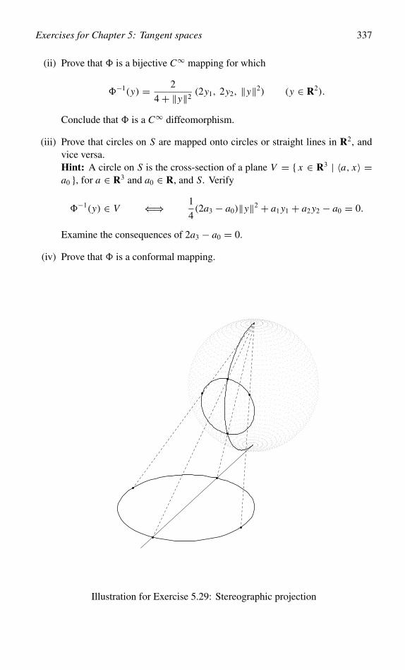
Exercises for Chapter 5: Tangent spaces 337
(ii) Prove that � is a bijective C∞ mapping for which
�−1(y) = 2
4+ ‖y‖2(2y1, 2y2, ‖y‖2) (y ∈ R2).
Conclude that � is a C∞ diffeomorphism.
(iii) Prove that circles on S are mapped onto circles or straight lines in R2, andvice versa.Hint: A circle on S is the cross-section of a plane V = { x ∈ R3 | 〈a, x〉 =a0 }, for a ∈ R3 and a0 ∈ R, and S. Verify
�−1(y) ∈ V ⇐⇒ 1
4(2a3 − a0)‖y‖2 + a1 y1 + a2 y2 − a0 = 0.
Examine the consequences of 2a3 − a0 = 0.
(iv) Prove that � is a conformal mapping.
Illustration for Exercise 5.29: Stereographic projection
338 Exercises for Chapter 5: Tangent spaces
Exercise 5.30 (Course of constant compass heading – sequel to Exercise 0.7– needed for Exercise 5.31). Let D = ]−π, π [ × ]−π
2 ,π2
[ ⊂ R2 and letφ : D → S2 = { x ∈ R3 | ‖x‖ = 1 } be the C1 embedding from Exercise 4.5with φ(α, θ) = (cosα cos θ, sin α cos θ, sin θ). Assume δ : I → D with δ(t) =(α(t), θ(t)) is a C1 curve, then γ := φ ◦ δ : I → S2 is a C1 curve on S2. Let t ∈ Iand let
µ : θ �→ (cosα(t) cos θ, sin α(t) cos θ, sin θ)
be the meridian on S2 given by α = α(t) and γ (t) ∈ im(µ).
(i) Prove 〈 γ ′(t), µ′(θ(t)) 〉 = θ ′(t).
(ii) Show that the angle β at the point γ (t) between the curve γ and the meridianµ is given by
cosβ = θ ′(t)√cos2 θ(t) α′(t)2 + θ ′(t)2
.
By definition, a loxodrome is a curve γ on S2 which makes a constant angle β withall meridians on S2 (λοξ�ς means skew, and � δρ�µος means course).
(iii) Prove that for a loxodrome γ (t) = φ(α(t), θ(t)) one has
α′(t) = ± tan β1
cos θ(t)θ ′(t).
(iv) Now use Exercise 0.7 to prove that γ defines a loxodrome if
α(t)+ c = ± tan β log tan1
2
(θ(t)+ π
2
).
Here the constant of integration c is determined by the requirement thatφ(α(t), θ(t)) = γ (t).
Exercise 5.31 (Mercator projection of sphere onto cylinder – sequel to Exer-cises 0.7 and 5.30 – needed for Exercise 5.51). Let the notation be that of Exer-cise 5.30. The result in part (iv) of that exercise suggests the following definitionfor the mapping � : D → E := ]−π, π [ × R:
�(α, θ) =(α, log tan
(θ2+ π
4
))=: (α, τ ).
(i) Prove that det D�(α, θ) = 1cos θ = 0, and that � : D → E is a C1 diffeo-
morphism.
Exercises for Chapter 5: Tangent spaces 339
(ii) Use the formulae from Exercise 0.7 to prove
sin θ = tanh τ, cos θ = 1
cosh τ.
Here cosh τ = 12 (e
τ + e−τ ), sinh τ = 12 (e
τ − e−τ ), tanh τ = sinh τcosh τ .
Now define the C1 parametrization
ψ : E → S2 by ψ(α, τ) =( cosα
cosh τ,
sin α
cosh τ, tanh τ
).
The inverse ψ−1 : S2 → E is said to be the Mercator projection of S2 onto]−π, π [ × R. Note that in the (α, τ )-coordinates for S2 a loxodrome is given bythe linear equation
α + c = ±τ tan β.
(iii) Verify that the Mercator projection: S2 \ { x ∈ R3 | x1 ≤ 0, x2 = 0 } →]−π, π [ × R is given by (see Exercise 3.7.(v))
x �→(
2 arctan( x2
x1 +√
x21 + x2
2
),
1
2log
(1+ x3
1− x3
)).
(iv) The stereographic projection of S2 onto the cylinder { x ∈ R3 | x21 + x2
2 =1 } � ]−π, π ]×R assigns to a point x ∈ S2 the nearest point of intersectionwith the cylinder of the straight line through x and the origin (compare withExercise 5.29). Show that the Mercator projection is not the same as thisstereographic projection. Yet more exactly, prove the following assertion. Ifx �→ (α, ξ) ∈ ]−π, π ] × R is the stereographic projection of x , then
x �→ (α, log(√ξ 2 + 1+ ξ))
is the Mercator projection of x . The Mercator projection, therefore, is not aprojection in the strict sense of the word projection.
(v) A slightly simpler construction for finding the Mercator coordinates (α, τ )of the point x = (cosα cos θ, sin α cos θ, sin θ) is as follows. Using Exer-cise 0.7 verify that r(cosα, sin α, 0)with r = tan( θ2 + π
4 ) is the stereographicprojection of x from (0, 0, 1) onto the equatorial plane { x ∈ R3 | x3 = 0 }.Thus x �→ (α, log r) is the Mercator projection of x .
(vi) Prove ⟨ ∂ψ∂α
(α, τ),∂ψ
∂α(α, τ)
⟩=
⟨ ∂ψ∂τ
(α, τ ),∂ψ
∂τ(α, τ )
⟩= 1
cosh2 τ,
⟨ ∂ψ∂α
(α, τ),∂ψ
∂τ(α, τ )
⟩= 0.
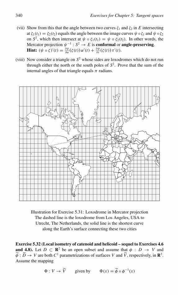
340 Exercises for Chapter 5: Tangent spaces
(vii) Show from this that the angle between two curves ζ1 and ζ2 in E intersectingat ζ1(t1) = ζ2(t2) equals the angle between the image curvesψ ◦ζ1 andψ ◦ζ2
on S2, which then intersect at ψ ◦ ζ1(t1) = ψ ◦ ζ2(t2). In other words, theMercator projection ψ−1 : S2 → E is conformal or angle-preserving.Hint: (ψ ◦ ζ )′(t) = ∂ψ
∂α(ζ(t))α′(t)+ ∂ψ
∂τ(ζ(t)) τ ′(t).
(viii) Now consider a triangle on S2 whose sides are loxodromes which do not runthrough either the north or the south poles of S2. Prove that the sum of theinternal angles of that triangle equals π radians.
Illustration for Exercise 5.31: Loxodrome in Mercator projectionThe dashed line is the loxodrome from Los Angeles, USA toUtrecht, The Netherlands, the solid line is the shortest curve
along the Earth’s surface connecting these two cities
Exercise 5.32 (Local isometry of catenoid and helicoid – sequel to Exercises 4.6and 4.8). Let D ⊂ R2 be an open subset and assume that φ : D → V andφ : D → V are both C1 parametrizations of surfaces V and V , respectively, in R3.Assume the mapping
� : V → V given by �(x) = φ ◦ φ−1(x)
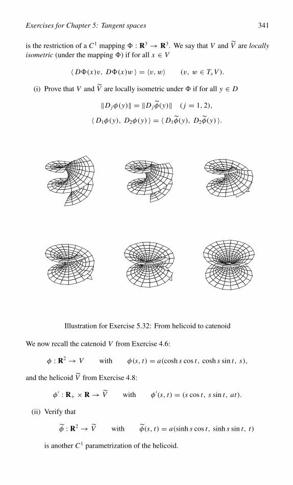
Exercises for Chapter 5: Tangent spaces 341
is the restriction of a C1 mapping � : R3 → R3. We say that V and V are locallyisometric (under the mapping �) if for all x ∈ V
〈 D�(x)v, D�(x)w 〉 = 〈v,w〉 (v, w ∈ Tx V ).
(i) Prove that V and V are locally isometric under � if for all y ∈ D
‖D jφ(y)‖ = ‖D j φ(y)‖ ( j = 1, 2),
〈 D1φ(y), D2φ(y) 〉 = 〈 D1φ(y), D2φ(y) 〉.
Illustration for Exercise 5.32: From helicoid to catenoid
We now recall the catenoid V from Exercise 4.6:
φ : R2 → V with φ(s, t) = a(cosh s cos t, cosh s sin t, s),
and the helicoid V from Exercise 4.8:
φ′ : R+ × R → V with φ′(s, t) = (s cos t, s sin t, at).
(ii) Verify that
φ : R2 → V with φ(s, t) = a(sinh s cos t, sinh s sin t, t)
is another C1 parametrization of the helicoid.
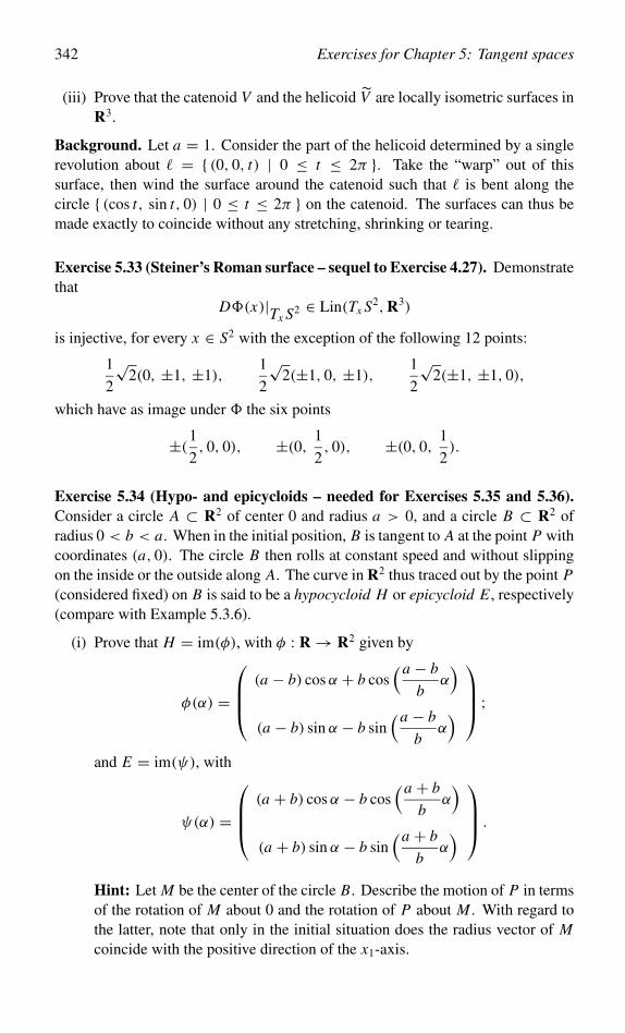
342 Exercises for Chapter 5: Tangent spaces
(iii) Prove that the catenoid V and the helicoid V are locally isometric surfaces inR3.
Background. Let a = 1. Consider the part of the helicoid determined by a singlerevolution about " = { (0, 0, t) | 0 ≤ t ≤ 2π }. Take the “warp” out of thissurface, then wind the surface around the catenoid such that " is bent along thecircle { (cos t, sin t, 0) | 0 ≤ t ≤ 2π } on the catenoid. The surfaces can thus bemade exactly to coincide without any stretching, shrinking or tearing.
Exercise 5.33 (Steiner’s Roman surface – sequel to Exercise 4.27). Demonstratethat
D�(x)|Tx S2 ∈ Lin(Tx S2,R3)
is injective, for every x ∈ S2 with the exception of the following 12 points:
1
2
√2(0, ±1, ±1),
1
2
√2(±1, 0, ±1),
1
2
√2(±1, ±1, 0),
which have as image under � the six points
±(1
2, 0, 0), ±(0, 1
2, 0), ±(0, 0,
1
2).
Exercise 5.34 (Hypo- and epicycloids – needed for Exercises 5.35 and 5.36).Consider a circle A ⊂ R2 of center 0 and radius a > 0, and a circle B ⊂ R2 ofradius 0 < b < a. When in the initial position, B is tangent to A at the point P withcoordinates (a, 0). The circle B then rolls at constant speed and without slippingon the inside or the outside along A. The curve in R2 thus traced out by the point P(considered fixed) on B is said to be a hypocycloid H or epicycloid E , respectively(compare with Example 5.3.6).
(i) Prove that H = im(φ), with φ : R → R2 given by
φ(α) =
(a − b) cosα + b cos(a − b
bα)
(a − b) sin α − b sin(a − b
bα)
;and E = im(ψ), with
ψ(α) =
(a + b) cosα − b cos(a + b
bα)
(a + b) sin α − b sin(a + b
bα)
.
Hint: Let M be the center of the circle B. Describe the motion of P in termsof the rotation of M about 0 and the rotation of P about M . With regard tothe latter, note that only in the initial situation does the radius vector of Mcoincide with the positive direction of the x1-axis.
Exercises for Chapter 5: Tangent spaces 343
a
2a
Illustration for Exercise 5.34.(ii): Nephroid
Note that the cardioid from Exercise 3.43 is an epicycloid for which a = b. Anepicycloid for which b = 1
2 a is said to be a nephroid (� νεφρ�ς = kidneys), and isgiven by
ν(α) = 1
2a( 3 cosα − cos 3α
3 sin α − sin 3α
).
(ii) Prove that the nephroid is a C∞ submanifold in R2 of dimension 1 at all ofits points, with the exception of the points (a, 0) and (−a, 0); and that thecurve has ordinary cusps at these points.Hint: We have
ν(α) =( a
0
)+
( 32 aα2 +O(α4)
2aα3 +O(α4)
), α→ 0.
Exercise 5.35 (Steiner’s hypocycloid – sequel to Exercise 5.34 – needed forExercise 8.6). A special case of the hypocycloid H occurs when b = 1
3 a:
φ(α) = b( 2 cosα + cos 2α
2 sin α − sin 2α
).
Define Cr = { r(cos θ, sin θ) ∈ R2 | θ ∈ R }, for r > 0.
(i) Prove that ‖φ(α)‖ = b√
5+ 4 cos 3α. Conclude that there are no pointsof H outside Ca , nor inside Cb, while H ∩ Ca and H ∩ Cb are given by,respectively,
{φ(0), φ(2
3π), φ(
4
3π) }, {φ(1
3π), φ(π), φ(
5
3π) }.
344 Exercises for Chapter 5: Tangent spaces
(ii) Prove thatφ is not an immersion at the pointsα ∈ R for whichφ(α) ∈ H∩Ca .
(iii) Prove that the geometric tangent line l(α) to H in φ(α) ∈ H \Ca is given by
l(α) = { h ∈ R2 | h1 sin1
2α + h2 cos
1
2α = b sin
3
2α }.
(iv) Show that H and Cb have coincident geometric tangent lines at the points ofH ∩ Cb.
We say that Cb is the incircle of H .
(v) Prove that H ∩ l(α) consists of the three points
x (0)(α) := φ(α), x (1)(α) := φ(π − 1
2α),
x (2)(α) := φ(2π − 1
2α) = φ(−1
2α).
(vi) Establish for which α ∈ R one has x (i)(α) = x ( j)(α), with i , j ∈ {0, 1, 2}.Conclude that H has ordinary cusps at the points of H ∩Ca , and corroboratethis by Taylor expansion.
(vii) Prove that for all α ∈ R
‖x (1)(α)− x (2)(α)‖ = 4b, ‖1
2(x (1)(α)+ x (2)(α))‖ = b.
That is, the segment of l(α) lying between those points of intersection withH that are different from φ(α) is of constant length 4b, and the midpoint ofthat segment lies on the incircle of H .
(viii) Prove that for φ(α) ∈ H \ Ca the geometric tangent lines at x (1)(α) andx (2)(α) are mutually orthogonal, intersecting at− 1
2 (x (1)(α)+ x (2)(α)) ∈ Cb.
Exercise 5.36 (Elimination theory: equations for hypo- and epicycloid – sequelto Exercises 5.34 and 5.35 - Needed for Exercise 5.37). Let the notation be asin Exercise 5.34. Let C be a hypocycloid or epicycloid, that is, C = im(φ) orC = im(ψ), and let β = a∓b
b α. Assume there exists m ∈ N such that β = mα.Then the coordinates (x1, x2) of x ∈ C ⊂ R2 satisfy a polynomial equation; wenow proceed to find the equation by means of the following elimination theory.
We commence by parametrizing the unit circle (save one point) without gonio-metric functions as follows. We choose a special point a = (−1, 0) on the unitcircle; then for every t ∈ R the line through a of slope t , given by x2 = t (x1 + 1),intersects with the circle at precisely one other point. The quadratic equation
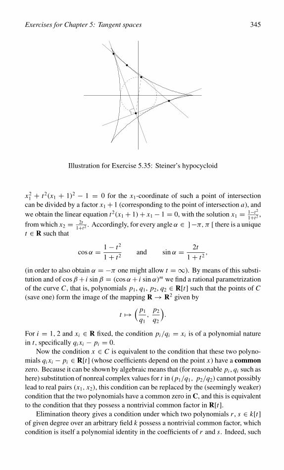
Exercises for Chapter 5: Tangent spaces 345
Illustration for Exercise 5.35: Steiner’s hypocycloid
x21 + t2(x1 + 1)2 − 1 = 0 for the x1-coordinate of such a point of intersection
can be divided by a factor x1+ 1 (corresponding to the point of intersection a), andwe obtain the linear equation t2(x1+ 1)+ x1− 1 = 0, with the solution x1 = 1−t2
1+t2 ,
from which x2 = 2t1+t2 . Accordingly, for every angle α ∈ ]−π, π [ there is a unique
t ∈ R such that
cosα = 1− t2
1+ t2and sin α = 2t
1+ t2,
(in order to also obtain α = −π one might allow t = ∞). By means of this substi-tution and of cosβ+ i sin β = (cosα+ i sin α)m we find a rational parametrizationof the curve C , that is, polynomials p1, q1, p2, q2 ∈ R[t] such that the points of C(save one) form the image of the mapping R → R2 given by
t �→( p1
q1,
p2
q2
).
For i = 1, 2 and xi ∈ R fixed, the condition pi/qi = xi is of a polynomial naturein t , specifically qi xi − pi = 0.
Now the condition x ∈ C is equivalent to the condition that these two polyno-mials qi xi − pi ∈ R[t] (whose coefficients depend on the point x) have a commonzero. Because it can be shown by algebraic means that (for reasonable pi , qi such ashere) substitution of nonreal complex values for t in (p1/q1, p2/q2) cannot possiblylead to real pairs (x1, x2), this condition can be replaced by the (seemingly weaker)condition that the two polynomials have a common zero in C, and this is equivalentto the condition that they possess a nontrivial common factor in R[t].
Elimination theory gives a condition under which two polynomials r , s ∈ k[t]of given degree over an arbitrary field k possess a nontrivial common factor, whichcondition is itself a polynomial identity in the coefficients of r and s. Indeed, such
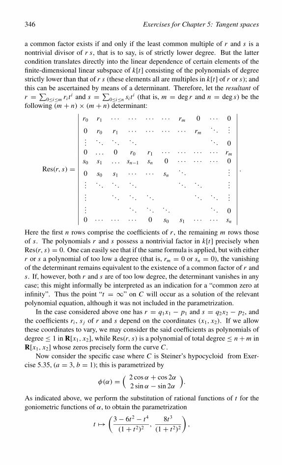
346 Exercises for Chapter 5: Tangent spaces
a common factor exists if and only if the least common multiple of r and s is anontrivial divisor of r s, that is to say, is of strictly lower degree. But the lattercondition translates directly into the linear dependence of certain elements of thefinite-dimensional linear subspace of k[t] consisting of the polynomials of degreestrictly lower than that of r s (these elements all are multiples in k[t] of r or s); andthis can be ascertained by means of a determinant. Therefore, let the resultant ofr = ∑
0≤i≤m ri t i and s = ∑0≤i≤n si t i (that is, m = deg r and n = deg s) be the
following (m + n)× (m + n) determinant:
Res(r, s) =
∣∣∣∣∣∣∣∣∣∣∣∣∣∣∣∣∣∣∣∣∣∣∣∣∣∣
r0 r1 · · · · · · · · · · · · rm 0 · · · 0
0 r0 r1 · · · · · · · · · · · · rm. . .
......
. . .. . .
. . .. . . 0
0 . . . 0 r0 r1 · · · · · · · · · · · · rm
s0 s1 . . . sn−1 sn 0 · · · · · · · · · 0
0 s0 s1 · · · · · · sn. . .
......
. . .. . .
. . .. . .
. . ....
.... . .
. . .. . .
. . .. . .
......
. . .. . .
. . .. . . 0
0 · · · · · · · · · 0 s0 s1 · · · · · · sn
∣∣∣∣∣∣∣∣∣∣∣∣∣∣∣∣∣∣∣∣∣∣∣∣∣∣
.
Here the first n rows comprise the coefficients of r , the remaining m rows thoseof s. The polynomials r and s possess a nontrivial factor in k[t] precisely whenRes(r, s) = 0. One can easily see that if the same formula is applied, but with eitherr or s a polynomial of too low a degree (that is, rm = 0 or sn = 0), the vanishingof the determinant remains equivalent to the existence of a common factor of r ands. If, however, both r and s are of too low degree, the determinant vanishes in anycase; this might informally be interpreted as an indication for a “common zero atinfinity”. Thus the point “t = ∞” on C will occur as a solution of the relevantpolynomial equation, although it was not included in the parametrization.
In the case considered above one has r = q1x1 − p1 and s = q2x2 − p2, andthe coefficients ri , s j of r and s depend on the coordinates (x1, x2). If we allowthese coordinates to vary, we may consider the said coefficients as polynomials ofdegree ≤ 1 in R[x1, x2], while Res(r, s) is a polynomial of total degree ≤ n+m inR[x1, x2] whose zeros precisely form the curve C .
Now consider the specific case where C is Steiner’s hypocycloid from Exer-cise 5.35, (a = 3, b = 1); this is parametrized by
φ(α) =( 2 cosα + cos 2α
2 sin α − sin 2α
).
As indicated above, we perform the substitution of rational functions of t for thegoniometric functions of α, to obtain the parametrization
t �→(
3− 6t2 − t4
(1+ t2)2,
8t3
(1+ t2)2
),
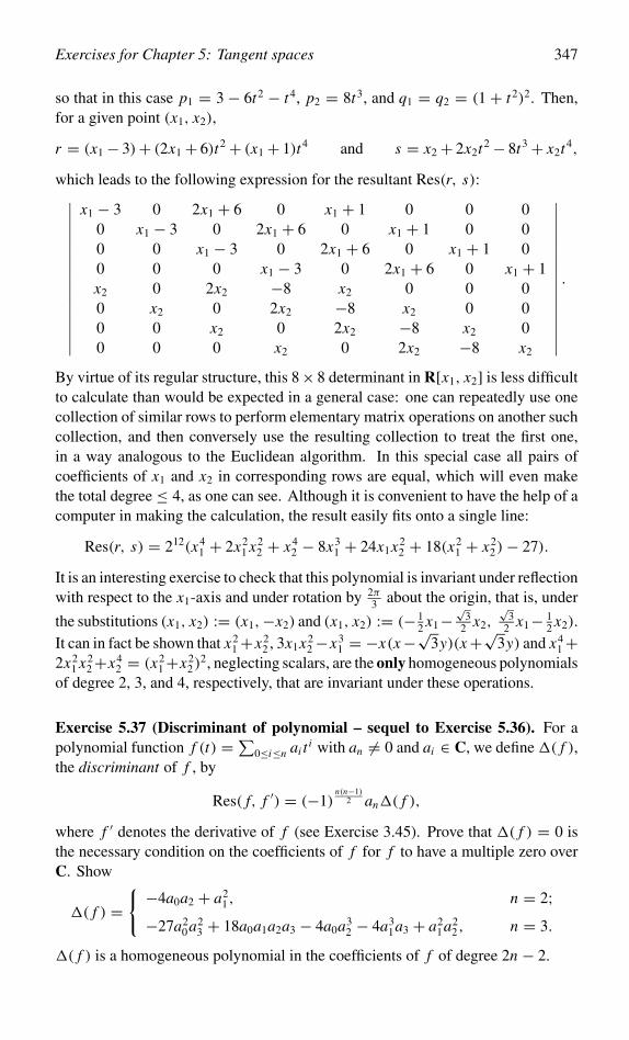
Exercises for Chapter 5: Tangent spaces 347
so that in this case p1 = 3 − 6t2 − t4, p2 = 8t3, and q1 = q2 = (1 + t2)2. Then,for a given point (x1, x2),
r = (x1− 3)+ (2x1+ 6)t2+ (x1+ 1)t4 and s = x2+ 2x2t2− 8t3+ x2t4,
which leads to the following expression for the resultant Res(r, s):∣∣∣∣∣∣∣∣∣∣∣∣∣∣∣∣
x1 − 3 0 2x1 + 6 0 x1 + 1 0 0 00 x1 − 3 0 2x1 + 6 0 x1 + 1 0 00 0 x1 − 3 0 2x1 + 6 0 x1 + 1 00 0 0 x1 − 3 0 2x1 + 6 0 x1 + 1x2 0 2x2 −8 x2 0 0 00 x2 0 2x2 −8 x2 0 00 0 x2 0 2x2 −8 x2 00 0 0 x2 0 2x2 −8 x2
∣∣∣∣∣∣∣∣∣∣∣∣∣∣∣∣.
By virtue of its regular structure, this 8× 8 determinant in R[x1, x2] is less difficultto calculate than would be expected in a general case: one can repeatedly use onecollection of similar rows to perform elementary matrix operations on another suchcollection, and then conversely use the resulting collection to treat the first one,in a way analogous to the Euclidean algorithm. In this special case all pairs ofcoefficients of x1 and x2 in corresponding rows are equal, which will even makethe total degree ≤ 4, as one can see. Although it is convenient to have the help of acomputer in making the calculation, the result easily fits onto a single line:
Res(r, s) = 212(x41 + 2x2
1 x22 + x4
2 − 8x31 + 24x1x2
2 + 18(x21 + x2
2)− 27).
It is an interesting exercise to check that this polynomial is invariant under reflectionwith respect to the x1-axis and under rotation by 2π
3 about the origin, that is, under
the substitutions (x1, x2) := (x1,−x2) and (x1, x2) := (− 12 x1−
√3
2 x2,√
32 x1− 1
2 x2).It can in fact be shown that x2
1+x22 , 3x1x2
2−x31 = −x(x−√3y)(x+√3y) and x4
1+2x2
1 x22+x4
2 = (x21+x2
2)2, neglecting scalars, are the only homogeneous polynomials
of degree 2, 3, and 4, respectively, that are invariant under these operations.
Exercise 5.37 (Discriminant of polynomial – sequel to Exercise 5.36). For apolynomial function f (t) =∑
0≤i≤n ai t i with an = 0 and ai ∈ C, we define �( f ),the discriminant of f , by
Res( f, f ′) = (−1)n(n−1)
2 an�( f ),
where f ′ denotes the derivative of f (see Exercise 3.45). Prove that �( f ) = 0 isthe necessary condition on the coefficients of f for f to have a multiple zero overC. Show
�( f ) ={ −4a0a2 + a2
1, n = 2;−27a2
0a23 + 18a0a1a2a3 − 4a0a3
2 − 4a31a3 + a2
1a22, n = 3.
�( f ) is a homogeneous polynomial in the coefficients of f of degree 2n − 2.
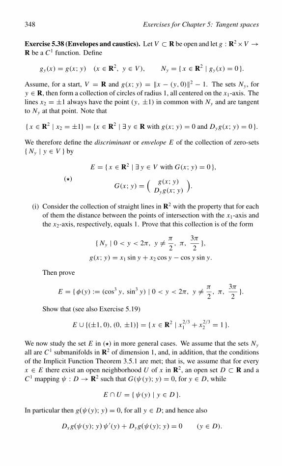
348 Exercises for Chapter 5: Tangent spaces
Exercise 5.38 (Envelopes and caustics). Let V ⊂ R be open and let g : R2×V →R be a C1 function. Define
gy(x) = g(x; y) (x ∈ R2, y ∈ V ), Ny = { x ∈ R2 | gy(x) = 0 }.Assume, for a start, V = R and g(x; y) = ‖x − (y, 0)‖2 − 1. The sets Ny , fory ∈ R, then form a collection of circles of radius 1, all centered on the x1-axis. Thelines x2 = ±1 always have the point (y, ±1) in common with Ny and are tangentto Ny at that point. Note that
{ x ∈ R2 | x2 = ±1} = {x ∈ R2 | ∃ y ∈ R with g(x; y) = 0 and Dyg(x; y) = 0 }.We therefore define the discriminant or envelope E of the collection of zero-sets{ Ny | y ∈ V } by
(�)
E = { x ∈ R2 | ∃ y ∈ V with G(x; y) = 0 },
G(x; y) =( g(x; y)
Dyg(x; y)
).
(i) Consider the collection of straight lines in R2 with the property that for eachof them the distance between the points of intersection with the x1-axis andthe x2-axis, respectively, equals 1. Prove that this collection is of the form
{ Ny | 0 < y < 2π, y = π
2, π,
3π
2},
g(x; y) = x1 sin y + x2 cos y − cos y sin y.
Then prove
E = {φ(y) := (cos3 y, sin3 y) | 0 < y < 2π, y = π
2, π,
3π
2}.
Show that (see also Exercise 5.19)
E ∪ {(±1, 0), (0, ±1)} = { x ∈ R2 | x2/31 + x2/3
2 = 1 }.
We now study the set E in (�) in more general cases. We assume that the sets Ny
all are C1 submanifolds in R2 of dimension 1, and, in addition, that the conditionsof the Implicit Function Theorem 3.5.1 are met; that is, we assume that for everyx ∈ E there exist an open neighborhood U of x in R2, an open set D ⊂ R and aC1 mapping ψ : D → R2 such that G(ψ(y); y) = 0, for y ∈ D, while
E ∩U = {ψ(y) | y ∈ D }.In particular then g(ψ(y); y) = 0, for all y ∈ D; and hence also
Dx g(ψ(y); y)ψ ′(y)+ Dyg(ψ(y); y) = 0 (y ∈ D).
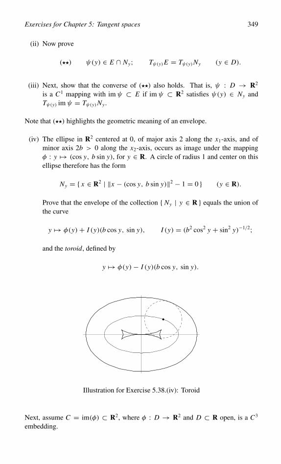
Exercises for Chapter 5: Tangent spaces 349
(ii) Now prove
(��) ψ(y) ∈ E ∩ Ny; Tψ(y)E = Tψ(y)Ny (y ∈ D).
(iii) Next, show that the converse of (��) also holds. That is, ψ : D → R2
is a C1 mapping with imψ ⊂ E if imψ ⊂ R2 satisfies ψ(y) ∈ Ny andTψ(y) imψ = Tψ(y)Ny .
Note that (��) highlights the geometric meaning of an envelope.
(iv) The ellipse in R2 centered at 0, of major axis 2 along the x1-axis, and ofminor axis 2b > 0 along the x2-axis, occurs as image under the mappingφ : y �→ (cos y, b sin y), for y ∈ R. A circle of radius 1 and center on thisellipse therefore has the form
Ny = { x ∈ R2 | ‖x − (cos y, b sin y)‖2 − 1 = 0 } (y ∈ R).
Prove that the envelope of the collection { Ny | y ∈ R } equals the union ofthe curve
y �→ φ(y)+ I (y)(b cos y, sin y), I (y) = (b2 cos2 y + sin2 y)−1/2;
and the toroid, defined by
y �→ φ(y)− I (y)(b cos y, sin y).
Illustration for Exercise 5.38.(iv): Toroid
Next, assume C = im(φ) ⊂ R2, where φ : D → R2 and D ⊂ R open, is a C3
embedding.
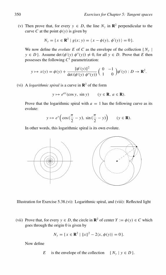
350 Exercises for Chapter 5: Tangent spaces
(v) Then prove that, for every y ∈ D, the line Ny in R2 perpendicular to thecurve C at the point φ(y) is given by
Ny = { x ∈ R2 | g(x; y) = 〈 x − φ(y), φ′(y) 〉 = 0 }.We now define the evolute E of C as the envelope of the collection { Ny |y ∈ D }. Assume det (φ′(y) φ′′(y)) = 0, for all y ∈ D. Prove that E thenpossesses the following C1 parametrization:
y �→ x(y) = φ(y)+ ‖φ′(y)‖2
det (φ′(y) φ′′(y))
( 0 −11 0
)φ′(y) : D → R2.
(vi) A logarithmic spiral is a curve in R2 of the form
y �→ eay(cos y, sin y) (y ∈ R, a ∈ R).
Prove that the logarithmic spiral with a = 1 has the following curve as itsevolute:
y �→ ey(
cos (π
2− y), sin (
π
2− y)
)(y ∈ R).
In other words, this logarithmic spiral is its own evolute.
Illustration for Exercise 5.38.(vi): Logarithmic spiral, and (viii): Reflected light
(vii) Prove that, for every y ∈ D, the circle in R2 of center Y := φ(y) ∈ C whichgoes through the origin 0 is given by
Ny = { x ∈ R2 | ‖x‖2 − 2〈x, φ(y)〉 = 0 }.Now define
E is the envelope of the collection { Ny | y ∈ D }.
Exercises for Chapter 5: Tangent spaces 351
Check that the point X := x ∈ R2 lying on E and parametrized by y satisfies
x ∈ Ny and 〈x, φ′(y)〉 = 0.
That is, the line segments Y O and Y X are of equal length and the line segmentO X is orthogonal to the tangent line at Y to C . Let L y ⊂ R2 be the straightline through Y and X . Then the ultimate course of a light ray starting fromO and reflected at Y by the curve C will be along a part of L y . Therefore,the envelope of the collection { L y | y ∈ D } is said to be the caustic of Crelative to O ( κα�σις = sun’s heat, burning). Since the tangent line at X to Ecoincides with the tangent line at X to the circle Ny , the line L y is orthogonalto E . Consequently, the caustic of C relative to O is the evolute of E .
(viii) Consider the circle in R2 of center 0 and radius a > 0, and the collectionof straight lines in R2 parallel to the x1-axis and at a distance ≤ a from thataxis. Assume that these lines are reflected by the circle in such a way that theangle between the incident line and the normal equals the angle between thereflected line and the normal. Prove that a reflected line is of the form Nα,for α ∈ R, where
Nα = { x ∈ R2 | x2 − x1 tan 2α + a cosα tan 2α − a sin α = 0 }.Prove that the envelope of the collection { Nα | α ∈ R } is given by the curve
α �→ 1
4a( 3 cosα − cos 3α
3 sin α − sin 3α
)= 1
2a( cosα(3− 2 cos2 α)
2 sin3 α
).
Background. Note that this is a nephroid from Exercise 5.34. The causticof sunlight reflected by the inner wall of a teacup of radius a is traced out bya point on a circle of radius 1
4 a when this circle rolls on the outside along acircle of radius 1
2 a.
Exercise 5.39 (Geometric–arithmetic and Kantorovich’s inequalities – neededfor Exercise 7.55).
(i) Shownn
∏1≤ j≤n
x2j ≤ ‖x‖2n (x ∈ Rn).
(ii) Assume that a1, . . . , an in R are nonnegative. Prove the geometric–arithmeticinequality ( ∏
1≤ j≤n
a j
)1/n ≤ a := 1
n
∑1≤ j≤n
a j .
Hint: Write a j = nax2j .
352 Exercises for Chapter 5: Tangent spaces
Let � ⊂ R2 be a triangle of area O and perimeter l.
(iii) (Sequel to Exercise 5.25). Prove by means of this exercise and part (ii) theisoperimetric inequality for �:
O ≤ l2
12√
3,
where equality obtains if and only if � is equilateral.
Assume that t1, . . . , tn ∈ R are nonnegative and satisfy t1 + · · · + tn = 1. Further-more, let 0 < m < M and suppose x j ∈ R satisfy m ≤ x j ≤ M for all 1 ≤ j ≤ n.Then we have Kantorovich’s inequality( ∑
1≤ j≤n
t j x j
)( ∑1≤ j≤n
t j x−1j
)≤ (m + M)2
4m M,
which we shall prove in three steps.
(iv) Verify that the inequality remains unchanged if we replace every x j by λ x j
with λ > 0. Conclude we may assume m M = 1, and hence 0 < m < 1.
(v) Determine the extrema of the function x �→ x + x−1 on I = [m, m−1 ]; nextshow x + x−1 ≤ m + M for x ∈ I , and deduce∑
1≤ j≤n
t j x j +∑
1≤ j≤n
t j x−1j ≤ m + M.
(vi) Verify that Kantorovich’s inequality follows from the geometric–arithmeticinequality.
Exercise 5.40. Let C be the cardioid from Exercise 3.43. Calculate the criticalpoints of the restriction to C of the function f (x, y) = y, in other words find thepoints where the tangent line to C is horizontal.
Exercise 5.41 (Hölder’s, Minkowski’s and Young’s inequalities – needed forExercises 6.73 and 6.75). For p ≥ 1 and x ∈ Rn we define
‖x‖p =( ∑
1≤ j≤n
|x j |p)1/p
.
Now assume that p ≥ 1 and q ≥ 1 satisfy
1
p+ 1
q= 1.
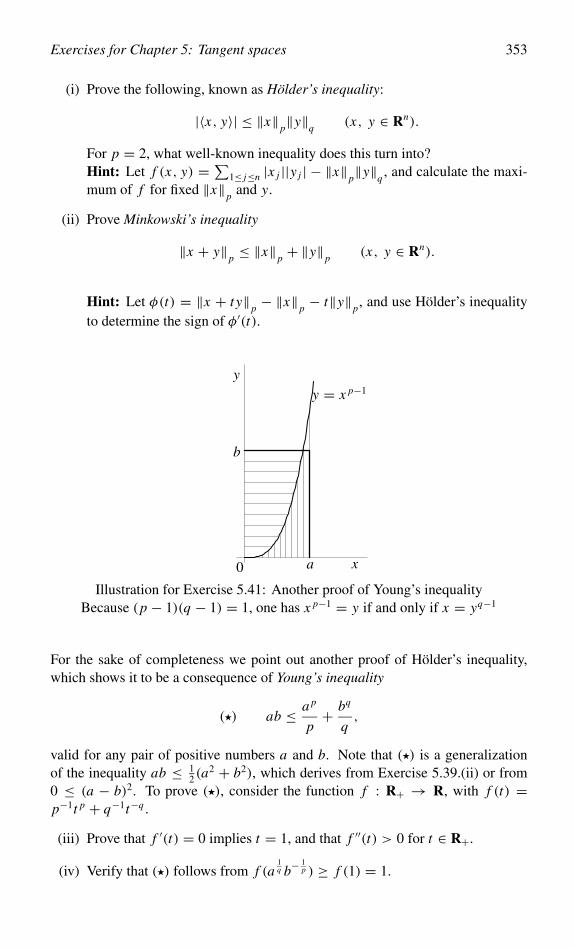
Exercises for Chapter 5: Tangent spaces 353
(i) Prove the following, known as Hölder’s inequality:
|〈x, y〉| ≤ ‖x‖p‖y‖q (x, y ∈ Rn).
For p = 2, what well-known inequality does this turn into?Hint: Let f (x, y) = ∑
1≤ j≤n |x j ||y j | − ‖x‖p‖y‖q , and calculate the maxi-mum of f for fixed ‖x‖p and y.
(ii) Prove Minkowski’s inequality
‖x + y‖p ≤ ‖x‖p + ‖y‖p (x, y ∈ Rn).
Hint: Let φ(t) = ‖x + t y‖p − ‖x‖p − t‖y‖p, and use Hölder’s inequalityto determine the sign of φ′(t).
a
b
x
y
y = x p−1
0
Illustration for Exercise 5.41: Another proof of Young’s inequalityBecause (p − 1)(q − 1) = 1, one has x p−1 = y if and only if x = yq−1
For the sake of completeness we point out another proof of Hölder’s inequality,which shows it to be a consequence of Young’s inequality
(�) ab ≤ a p
p+ bq
q,
valid for any pair of positive numbers a and b. Note that (�) is a generalizationof the inequality ab ≤ 1
2 (a2 + b2), which derives from Exercise 5.39.(ii) or from
0 ≤ (a − b)2. To prove (�), consider the function f : R+ → R, with f (t) =p−1t p + q−1t−q .
(iii) Prove that f ′(t) = 0 implies t = 1, and that f ′′(t) > 0 for t ∈ R+.
(iv) Verify that (�) follows from f (a1q b−
1p ) ≥ f (1) = 1.
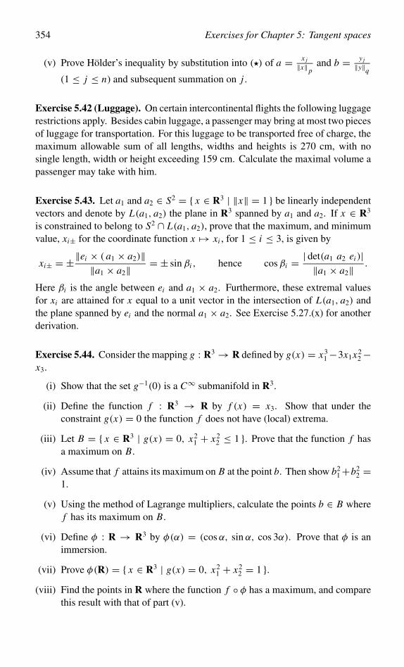
354 Exercises for Chapter 5: Tangent spaces
(v) Prove Hölder’s inequality by substitution into (�) of a = x j
‖x‖pand b = y j
‖y‖q(1 ≤ j ≤ n) and subsequent summation on j .
Exercise 5.42 (Luggage). On certain intercontinental flights the following luggagerestrictions apply. Besides cabin luggage, a passenger may bring at most two piecesof luggage for transportation. For this luggage to be transported free of charge, themaximum allowable sum of all lengths, widths and heights is 270 cm, with nosingle length, width or height exceeding 159 cm. Calculate the maximal volume apassenger may take with him.
Exercise 5.43. Let a1 and a2 ∈ S2 = { x ∈ R3 | ‖x‖ = 1 } be linearly independentvectors and denote by L(a1, a2) the plane in R3 spanned by a1 and a2. If x ∈ R3
is constrained to belong to S2 ∩ L(a1, a2), prove that the maximum, and minimumvalue, xi± for the coordinate function x �→ xi , for 1 ≤ i ≤ 3, is given by
xi± = ±‖ei × ( a1 × a2)‖‖a1 × a2‖ = ± sin βi , hence cosβi = | det(a1 a2 ei )|
‖a1 × a2‖ .
Here βi is the angle between ei and a1 × a2. Furthermore, these extremal valuesfor xi are attained for x equal to a unit vector in the intersection of L(a1, a2) andthe plane spanned by ei and the normal a1 × a2. See Exercise 5.27.(x) for anotherderivation.
Exercise 5.44. Consider the mapping g : R3 → R defined by g(x) = x31−3x1x2
2−x3.
(i) Show that the set g−1(0) is a C∞ submanifold in R3.
(ii) Define the function f : R3 → R by f (x) = x3. Show that under theconstraint g(x) = 0 the function f does not have (local) extrema.
(iii) Let B = { x ∈ R3 | g(x) = 0, x21 + x2
2 ≤ 1 }. Prove that the function f hasa maximum on B.
(iv) Assume that f attains its maximum on B at the point b. Then show b21+b2
2 =1.
(v) Using the method of Lagrange multipliers, calculate the points b ∈ B wheref has its maximum on B.
(vi) Define φ : R → R3 by φ(α) = (cosα, sin α, cos 3α). Prove that φ is animmersion.
(vii) Prove φ(R) = { x ∈ R3 | g(x) = 0, x21 + x2
2 = 1 }.(viii) Find the points in R where the function f ◦ φ has a maximum, and compare
this result with that of part (v).
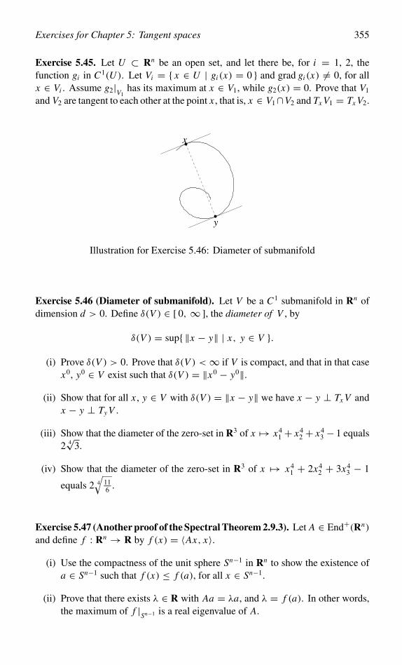
Exercises for Chapter 5: Tangent spaces 355
Exercise 5.45. Let U ⊂ Rn be an open set, and let there be, for i = 1, 2, thefunction gi in C1(U ). Let Vi = { x ∈ U | gi (x) = 0 } and grad gi (x) = 0, for allx ∈ Vi . Assume g2|V1
has its maximum at x ∈ V1, while g2(x) = 0. Prove that V1
and V2 are tangent to each other at the point x , that is, x ∈ V1∩V2 and Tx V1 = Tx V2.
x
y
Illustration for Exercise 5.46: Diameter of submanifold
Exercise 5.46 (Diameter of submanifold). Let V be a C1 submanifold in Rn ofdimension d > 0. Define δ(V ) ∈ [ 0, ∞], the diameter of V , by
δ(V ) = sup{ ‖x − y‖ | x, y ∈ V }.
(i) Prove δ(V ) > 0. Prove that δ(V ) <∞ if V is compact, and that in that casex0, y0 ∈ V exist such that δ(V ) = ‖x0 − y0‖.
(ii) Show that for all x , y ∈ V with δ(V ) = ‖x − y‖ we have x − y ⊥ Tx V andx − y ⊥ Ty V .
(iii) Show that the diameter of the zero-set in R3 of x �→ x41 + x4
2 + x43 − 1 equals
2 4√
3.
(iv) Show that the diameter of the zero-set in R3 of x �→ x41 + 2x4
2 + 3x43 − 1
equals 2 4
√116 .
Exercise 5.47 (Another proof of the Spectral Theorem 2.9.3). Let A ∈ End+(Rn)
and define f : Rn → R by f (x) = 〈Ax, x〉.(i) Use the compactness of the unit sphere Sn−1 in Rn to show the existence of
a ∈ Sn−1 such that f (x) ≤ f (a), for all x ∈ Sn−1.
(ii) Prove that there exists λ ∈ R with Aa = λa, and λ = f (a). In other words,the maximum of f |Sn−1 is a real eigenvalue of A.
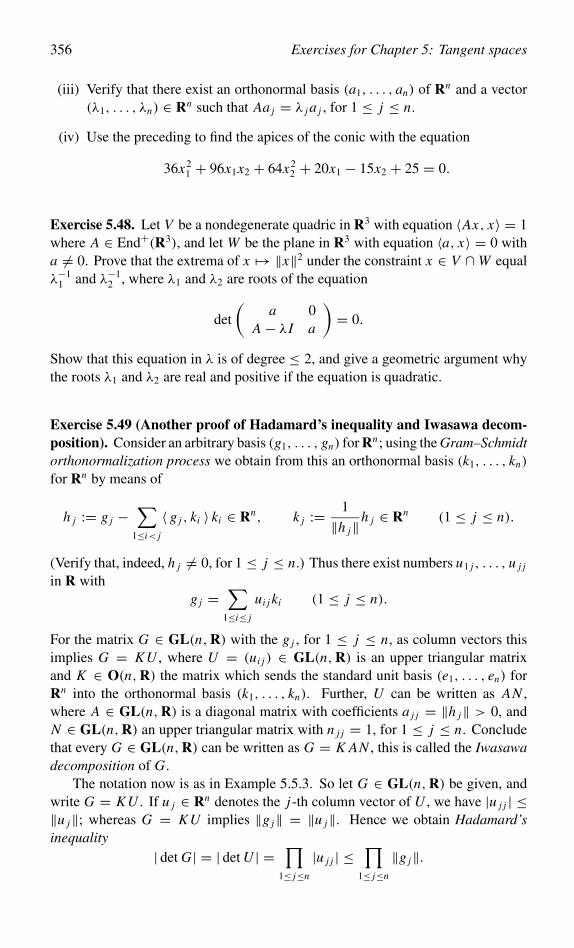
356 Exercises for Chapter 5: Tangent spaces
(iii) Verify that there exist an orthonormal basis (a1, . . . , an) of Rn and a vector(λ1, . . . , λn) ∈ Rn such that Aa j = λ j a j , for 1 ≤ j ≤ n.
(iv) Use the preceding to find the apices of the conic with the equation
36x21 + 96x1x2 + 64x2
2 + 20x1 − 15x2 + 25 = 0.
Exercise 5.48. Let V be a nondegenerate quadric in R3 with equation 〈Ax, x〉 = 1where A ∈ End+(R3), and let W be the plane in R3 with equation 〈a, x〉 = 0 witha = 0. Prove that the extrema of x �→ ‖x‖2 under the constraint x ∈ V ∩W equalλ−1
1 and λ−12 , where λ1 and λ2 are roots of the equation
det
(a 0
A − λI a
)= 0.
Show that this equation in λ is of degree ≤ 2, and give a geometric argument whythe roots λ1 and λ2 are real and positive if the equation is quadratic.
Exercise 5.49 (Another proof of Hadamard’s inequality and Iwasawa decom-position). Consider an arbitrary basis (g1, . . . , gn) for Rn; using the Gram–Schmidtorthonormalization process we obtain from this an orthonormal basis (k1, . . . , kn)
for Rn by means of
h j := g j −∑
1≤i< j
〈 g j , ki 〉 ki ∈ Rn, k j := 1
‖h j‖h j ∈ Rn (1 ≤ j ≤ n).
(Verify that, indeed, h j = 0, for 1 ≤ j ≤ n.) Thus there exist numbers u1 j , . . . , u j j
in R withg j =
∑1≤i≤ j
ui j ki (1 ≤ j ≤ n).
For the matrix G ∈ GL(n,R) with the g j , for 1 ≤ j ≤ n, as column vectors thisimplies G = KU , where U = (ui j ) ∈ GL(n,R) is an upper triangular matrixand K ∈ O(n,R) the matrix which sends the standard unit basis (e1, . . . , en) forRn into the orthonormal basis (k1, . . . , kn). Further, U can be written as AN ,where A ∈ GL(n,R) is a diagonal matrix with coefficients a j j = ‖h j‖ > 0, andN ∈ GL(n,R) an upper triangular matrix with n j j = 1, for 1 ≤ j ≤ n. Concludethat every G ∈ GL(n,R) can be written as G = K AN , this is called the Iwasawadecomposition of G.
The notation now is as in Example 5.5.3. So let G ∈ GL(n,R) be given, andwrite G = KU . If u j ∈ Rn denotes the j-th column vector of U , we have |u j j | ≤‖u j‖; whereas G = KU implies ‖g j‖ = ‖u j‖. Hence we obtain Hadamard’sinequality
| det G| = | det U | =∏
1≤ j≤n
|u j j | ≤∏
1≤ j≤n
‖g j‖.
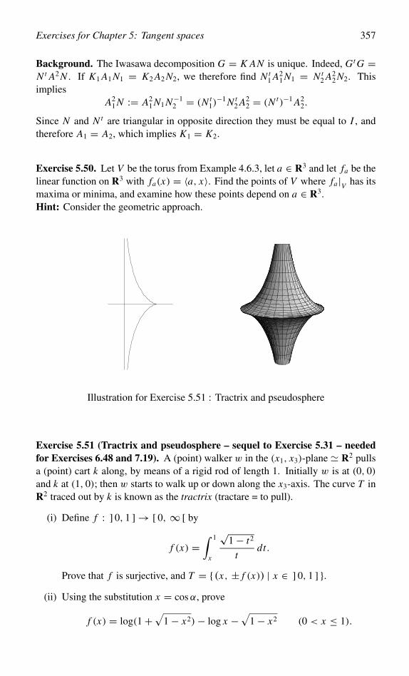
Exercises for Chapter 5: Tangent spaces 357
Background. The Iwasawa decomposition G = K AN is unique. Indeed, Gt G =N t A2 N . If K1 A1 N1 = K2 A2 N2, we therefore find N t
1 A21 N1 = N t
2 A22 N2. This
impliesA2
1 N := A21 N1 N−1
2 = (N t1)−1 N t
2 A22 = (N t)−1 A2
2.
Since N and N t are triangular in opposite direction they must be equal to I , andtherefore A1 = A2, which implies K1 = K2.
Exercise 5.50. Let V be the torus from Example 4.6.3, let a ∈ R3 and let fa be thelinear function on R3 with fa(x) = 〈a, x〉. Find the points of V where fa|V has itsmaxima or minima, and examine how these points depend on a ∈ R3.Hint: Consider the geometric approach.
Illustration for Exercise 5.51 : Tractrix and pseudosphere
Exercise 5.51 (Tractrix and pseudosphere – sequel to Exercise 5.31 – neededfor Exercises 6.48 and 7.19). A (point) walker w in the (x1, x3)-plane � R2 pullsa (point) cart k along, by means of a rigid rod of length 1. Initially w is at (0, 0)and k at (1, 0); then w starts to walk up or down along the x3-axis. The curve T inR2 traced out by k is known as the tractrix (tractare = to pull).
(i) Define f : ] 0, 1 ] → [ 0, ∞ [ by
f (x) =∫ 1
x
√1− t2
tdt.
Prove that f is surjective, and T = { (x, ± f (x)) | x ∈ ] 0, 1 ] }.(ii) Using the substitution x = cosα, prove
f (x) = log(1+√
1− x2)− log x −√
1− x2 (0 < x ≤ 1).
358 Exercises for Chapter 5: Tangent spaces
Verify T = { (sin s, cos s + log tan s2 ) | 0 < s < π }. Conclude
T ={ (
cos θ, − sin θ + log tan(θ
2+ π
4
)) ∣∣∣ − π
2< θ <
π
2
}.
Deduce that the x3-coordinate of w equals log tan( θ2 + π4 ) when the angle of
the rod with the horizontal direction is θ . Note that this gives a geometricalconstruction of the Mercator coordinates from Exercise 5.31 of a point on S2.
(iii) Show that T \ {(1, 0)} is a C∞ submanifold in R2 of dimension 1, and that Tis not a C∞ submanifold at (1, 0).
(iv) Let V be the surface of revolution in R3 obtained by revolving T \ {(1, 0)}about the x3-axis (see Exercise 4.6). Prove that every sphere in R3 of radius1 and center on the x3-axis orthogonally intersects with V .
(v) Show that V ⊂ im(φ), where φ(s, t) = (sin s cos t, sin s sin t, cos s +log tan 1
2 s). Prove
∂φ
∂s(s, t)× ∂φ
∂t(s, t) = cos s
− cos s cos t− cos s sin t
sin s
,
Dn(φ(s, t)) =( tan s 0
0 − cot s
).
Prove that the Gauss curvature of V equals −1 everywhere. Explain why Vis called the pseudosphere.
Exercise 5.52 (Curvature of planar curve and evolute).
(i) Let f : I → R be a C2 function. Show that the planar curve in R3
parametrized by t �→ (t, f (t), 0) has curvature
κ = | f ′′|(1+ f ′2)3/2
: I → [ 0, ∞ [ .
(ii) Let γ : I → R2 be a C2 embedding. Prove that the planar curve in R3
parametrized by t �→ (γ1(t), γ2(t), 0) has curvature
κ = | det(γ ′ γ ′′)|‖γ ′‖3
: I → [ 0, ∞ [ .
Exercises for Chapter 5: Tangent spaces 359
(iii) Let the notation be as in Exercise 5.38.(v). Show that the parametrization ofthe evolute E also can be written as
y �→ φ(y)+ 1
κ(y)N (y),
where κ(y) denotes the curvature of im(φ) at φ(y), and N (y) the normal toim(φ) at φ(y).
Exercise 5.53 (Curvature of ellipse or hyperbola – sequel to Exercise 5.24). Weuse the notation of that exercise. In particular, given 0 = ε ∈ R2 and 0 = d ∈ R,consider C = { x ∈ R2 | ‖x‖ = 〈x, ε〉 + d }. Suppose that R � t �→ x(t) ∈ R2 is aC2 curve with image equal to C . In the following we often write x instead of x(t)to simplify the notation, and similarly x ′ and x ′′.
(i) Prove by differentiation
〈 ε − 1
‖x‖ x, x ′ 〉 = 0, and deduce ε = 1
‖x‖ x + d
lJ x ′,
with J ∈ SO(2,R) as in Lemma 8.1.5 and l = det(x x ′) = −〈J x ′, x〉.(ii) From now on, assume C to be either an ellipse or a hyperbola. Applying part
(i), the definition of C and Exercise 5.24.(ii), show
(‖x‖ ‖x ′‖)2 = l2
d2‖x‖2
(1+ e2 − 2
〈x, ε〉‖x‖
)= ± l2
b2(2a‖x‖ − ‖x‖2).
(iii) Differentiate the identity in part (i) once more in order to obtain ‖x×x ′‖2
‖x‖3 =dl det(x ′ x ′′); in other words, det(x ′ x ′′) = l3
d‖x‖3 . Denoting by κ the curvatureof C , conclude on account of Formula (5.17) and part (ii)
κ = | det(x ′ x ′′)|‖x ′‖3
= 1
d
( | det(x x ′)|‖x‖ ‖x ′‖
)3
= ab
(± (2a‖x‖ − ‖x‖2))32
= b4
a2h3.
Here h = ba ( ± (2a‖x‖ − ‖x‖2))
12 is the distance between x ∈ C and the
point of intersection of the line perpendicular to C at x and of the focal axisRε. The sign± occurs as C is an ellipse or a hyperbola, respectively. For thelast equality, suppose ε = (e, 0) and deduce |x ′1| = l
dx2‖x‖ from part (i) using
that J 2 = −I .
Exercise 5.54 (Independence of curvature and torsion of parametrization).Prove directly that the formulae in (5.17) for the curvature and torsion of a curve inR3 are independent of the choice of the parametrization γ : I → R3.
360 Exercises for Chapter 5: Tangent spaces
Hint: Let γ : I → R3 be another parametrization and assume γ (t) = γ (t), witht ∈ I and t ∈ I ; then t = (γ−1 ◦ γ )(t) =: �(t). Application of the chain rule toγ = γ ◦� on I therefore gives, for t ∈ I , t = �(t) ∈ I ,
γ ′(t) = � ′(t) γ ′(t),
γ ′′(t) = � ′′(t) γ ′(t)+� ′(t)2 γ ′′(t),
γ ′′′(t) = · · · +� ′(t)3 γ ′′′(t).
Exercise 5.55 (Projections of curve). Let the notation be as in Section 5.8. Supposeγ : J → R3 to be a biregular C4 parametrization by arc length s starting at 0 ∈ J .Using a rotation in R3 we may assume that T (0), N (0), B(0) coincide with thestandard basis vectors e1, e2, e3 in R3.
(i) Set κ = κ(0), κ ′ = κ ′(0) and τ = τ(0). By means of the formulae ofFrenet–Serret prove
γ ′(0) =( 1
00
), γ ′′(0) =
( 0κ
0
), γ ′′′(0) =
( −κ2
κ ′κτ
).
(ii) Applying a translation in R3 we can arrange that γ (0) = 0. Using Taylorexpansion show
γ (s) = sγ ′(0)+ s2
2γ ′′(0)+ s3
6γ ′′′(0)+O(s4)
=
s − κ2
6s3
κ
2s2 + κ ′
6s3
κτ
6s3
+O(s4), s → 0.
Deduce
lims→0
γ2(s)
γ1(s)2= κ
2, lim
s→0
γ3(s)2
γ2(s)3= 2τ 2
9κ, lim
s→0
γ3(s)
γ1(s)3= κτ
6.
(iii) Show that the orthogonal projections of im(γ ) onto the following planes nearthe origin are approximated by the curves, respectively (here we supposeτ = 0) (see the Illustration for Exercise 4.28):
osculating, x2 = κ
2x2
1 , parabola;
normal, x23 =
2τ 2
9κx3
2 , semicubic parabola;rectifying, x3 = κτ
6x3
1 , cubic.
Exercises for Chapter 5: Tangent spaces 361
(iv) Prove that the parabola in the osculating plane in turn is approximated nearthe origin by the osculating circle with equation x2
1 + (x2 − 1κ)2 = 1
κ2 . Ingeneral, the osculating circle of im(γ ) at γ (s) is defined to be the circle inthe osculating plane at γ (s) that is tangent to im(γ ) at γ (s), has the samecurvature as im(γ ) at γ (s), and lies toward the concave or inner side of im(γ ).The osculating circle is centered at 1
κ(s) N (s) and has radius 1κ(s) (recall that
the osculating plane is a linear subspace, and not an affine plane containingγ (s)).
Exercise 5.56 (Geodesic). Let I ⊂ R denote an open interval, assume V to be aC2 hypersurface in Rn for which a continuous choice x �→ n(x) of a normal to Vat x ∈ V has been made, and let γ : I → V be a C2 mapping. Then γ is said tobe a geodesic in V if the acceleration γ ′′(t) ∈ Rn satisfies γ ′′(t) ⊥ Tγ (t)V , for allt ∈ I ; that is, the curve γ has no acceleration in the direction of V , and therefore itgoes “straight ahead” in V . In other words, γ ′′(t) is a scalar multiple of the normal(n ◦ γ )(t) to V at γ (t); and thus there is λ(t) ∈ R satisfying
γ ′′(t) = λ(t) (n ◦ γ )(t) (t ∈ I ).
(i) For every geodesic γ on the unit sphere Sn−1 of dimension n − 1, show thatthere exist a number a ∈ R and an orthogonal pair of unit vectors v1 andv2 ∈ Rn such that γ (t) = (cos at) v1 + (sin at) v2. For a = 0 these are greatcircles on Sn−1.
(ii) Using γ ′(t) ∈ Tγ (t)V , prove that we have, for a geodesic γ in V ,
λ(t) = 〈 γ ′′, (n ◦ γ ) 〉(t) = −〈 γ ′, (n ◦ γ )′ 〉(t) = −〈 γ ′, (Dn) ◦ γ · γ ′ 〉(t);
and deduce the following identity in C(I, Rn):
γ ′′ + 〈 γ ′, (Dn) ◦ γ · γ ′ 〉(n ◦ γ ) = 0.
(iii) Verify that the equation from part (ii) is equivalent to the following systemof second-order ordinary differential equations with variable coefficients:
γ ′′i +∑
1≤ j, k≤n
((ni D j nk) ◦ γ ) γ ′jγ′k = 0 (1 ≤ i ≤ n).
Background. By the existence theorem for the solutions of such differential equa-tions, for every point x ∈ V and every vector v ∈ Tx V there exists a geodesicγ : I → V with 0 ∈ I such that γ (0) = x and γ ′(0) = v; that is, through everypoint of V there is a geodesic passing in a prescribed direction.
362 Exercises for Chapter 5: Tangent spaces
(iv) Suppose n = 3. Show that any normal section of V is a geodesic.
Exercise 5.57 (Foucault’s pendulum). The swing plane of an ideal pendulum withsmall oscillations suspended over a point of the Earth at latitude θ rotates uniformlyabout the direction of gravity by an angle of −2π sin θ per day. This rotation is aconsequence of the rotation of the Earth about its axis. This we shall prove in anumber of steps.
We describe the surface of the Earth by the unit sphere S2. The position of theswing plane is completely determined by the location x of the point of suspensionand the unit tangent vector X (x) (up to a sign) given by the swing direction; that is
(�) x ∈ S2 and X (x) ∈ Tx S2 ⊂ R3, X (x) ∈ S2.
Furthermore, after a suitable choice of signs we assume that X : S2 → R3 is a C1
tangent vector field to S2. Now suppose x is located on the parallel determined bya fixed −π
2 ≤ θ ≤ π2 . More precisely, we assume x = γ (α) at the time α ∈ R,
where
γ : R → S2 and γ (α) = φ(α, θ) = (cosα cos θ, sin α cos θ, sin θ).
In other words, the Earth is supposed to be stationary and the point of suspension tobe moving with constant speed along the parallel. This angular motion being veryslow, the force associated with the curvilinear motion and felt by the pendulum isnegligible. Consequently, gravity is the only force felt by the pendulum and the solecause of change in its swing direction. Therefore (X ◦γ )′(α) ∈ R3 is perpendicularat γ (α) to the surface of the Earth, that is
(��) (X ◦ γ )′(α) ⊥ Tγ (α)S2 (α ∈ R).
(i) Verify that the following two vectors in R3 form a basis for Tγ (α)S2, forα ∈ R:
v1(α) = 1
cos θ
∂φ
∂α(α, θ) = (− sin α, cosα, 0) = 1
cos θγ ′(α),
v2(α) = ∂φ
∂θ(α, θ) = (− cosα sin θ, − sin α sin θ, cos θ).
(ii) Prove that the functions vi : R → R3 satisfy, for 1 ≤ i ≤ 2,
〈vi , vi 〉 = 1, 〈v′i , vi 〉 = 0, 〈v1, v2〉 = 0,
〈v′1, v2〉 = −〈v1, v′2〉 = sin θ.
Exercises for Chapter 5: Tangent spaces 363
(iii) Deduce from (�) and part (ii) that we can write
X ◦ γ = (cosβ) v1 + (sin β) v2 : R → R3,
whereβ(α) is the angle between the tangent vector (X◦γ )(α) and the parallel.
(iv) Show
(X ◦ γ )′ = −(β ′ sin β) v1 + (cosβ) v′1 + (β ′ cosβ) v2 + (sin β) v′2.
Now deduce from (��) and part (ii) that β : R → R has to satisfy thedifferential equation
β ′(α)+ sin θ = 0 (α ∈ R),
which has the solution
β(α)− β(α0) = (α0 − α) sin θ (α ∈ R).
In particular, β(α0 + 2π)− β(α0) = −2π sin θ .
Background. Angles are determined up to multiples of 2π . Therefore we maynormalize the angle of rotation of the swing plane by the condition that the anglebe small for small parallels; the angle then becomes 2π(1 − sin θ). According toExample 7.4.6 this is equal to the area of the cap of S2 bounded by the paralleldetermined by θ . (See also Exercises 8.10 and 8.45.)
The directions of the swing planes moving along the parallel are said to beparallel, because the instantaneous change of such a direction has no componentin the tangent plane to the sphere. More in general, let V be a manifold and x ∈ V .The element in the orthogonal group of the tangent space Tx V corresponding to thechange in direction of a vector in Tx V caused by parallel transport from the point xalong a closed curve in V is called the holonomy of V at x along the closed curve.This holonomy is determined by the curvature form of V (see Exercise 5.80).
Exercise 5.58 (Exponential of antisymmetric is special orthogonal in R3 – sequelto Exercises 4.22, 4.23 and 5.26 – needed for Exercises 5.59, 5.60, 5.67 and 5.68).The notation is that of Exercise 4.22. Let a ∈ S2 = { x ∈ R3 | ‖a‖ = 1 }, anddefine the cross product operator ra ∈ End(R3) by
ra x = a × x .
(i) Verify that the matrix in A(3,R), the linear subspace in Mat(3,R) of theantisymmetric matrices, of ra is given by (compare with Exercise 4.22.(iv)) 0 −a3 a2
a3 0 −a1
−a2 a1 0
.
364 Exercises for Chapter 5: Tangent spaces
Prove by Grassmann’s identity from Exercise 5.26.(ii), for n ∈ N and x ∈ R3,
r2na x = (−1)n(x − 〈 a, x 〉 a), r2n+1
a x = (−1)n a × x .
(ii) Let α ∈ R with 0 ≤ α ≤ π . Show the following identity of mappings inEnd(R3) (see Example 2.4.10):
eα ra =∑n∈N0
αn
n! rna : x �→ (1− cosα)〈 a, x 〉 a + (cosα) x + (sin α) a × x .
Prove eα ra a = a. Select x ∈ R3 satisfying 〈a, x〉 = 0 and ‖x‖ = 1 and show〈a, a× x〉 = 0 and ‖a× x‖ = 1. Deduce eα ra x = (cosα) x + (sin α) a× x .Use this to prove that
eα ra = Rα,a,
the rotation in R3 by the angle α about the axis a. In other words, we haveproved Euler’s formula from Exercise 4.22.(iii). In particular, show that theexponential mapping A(3,R)→ SO(3,R) is surjective. Furthermore, verifythe following identity of matrices:
expα
0 −a3 a2
a3 0 −a1
−a2 a1 0
= cosα I + (1− cosα) aat + sin α ra =
cosα + a21 c(α) −a3 sin α + a1a2 c(α) a2 sin α + a1a3 c(α)
a3 sin α + a1a2 c(α) cosα + a22 c(α) −a1 sin α + a2a3 c(α)
−a2 sin α + a1a3 c(α) a1 sin α + a2a3 c(α) cosα + a23 c(α)
,
where c(α) = 1− cosα.
(iii) Introduce p = (p0, p) ∈ R×R3 � R4 by (compare with Exercise 5.65.(ii))
p0 = cosα
2, p = sin
α
2a.
Verify that p ∈ S3 = { p ∈ R4 | p20 + ‖p‖2 = 1 }. Prove
Rα,a = R p : x �→ 2〈p, x〉 p + (p20 − ‖p‖2) x + 2p0 p × x (x ∈ R3),
and also that we have the following rational parametrization of a matrix inSO(3,R) (compare with Exercise 5.65.(iv)):
Rα,a = R p = (p20 − ‖p‖2)I + 2(ppt + p0rp)
= p2
0 + p21 − p2
2 − p23 2(p1 p2 − p0 p3) 2(p1 p3 + p0 p2)
2(p2 p1 + p0 p3) p20 − p2
1 + p22 − p2
3 2(p2 p3 − p0 p1)
2(p3 p1 − p0 p2) 2(p3 p2 + p0 p1) p20 − p2
1 − p22 + p2
3
.
Exercises for Chapter 5: Tangent spaces 365
Conversely, given p ∈ S3 we can reconstruct (α, a) with Rα,a = R p bymeans of
α = 2 arccos p0 = arccos(2p20 − 1), a = sgn(p0)
1
‖p‖ p.
Note that p and− p give the same result. The calculation of p ∈ S3 from thematrix R p above follows by means of
4p20 = 1+ tr R p, 4p0rp = R p − Rt
p.
If p0 = 0, we use (write R p = (Ri j ))
2p2i = 1+ Rii , 2pi p j = Ri j (1 ≤ i, j ≤ 3, i = j).
Because at least one pi = 0, this means that (p0, p) ∈ R4 is determined byR p to within a factor ±1.
(iv) Consider A = (ai j ) ∈ SO(3,R). Furthermore, let Ai j ∈ Mat(n − 1,R) bethe matrix obtained from A by deleting the i-th row and the j-th column,then det Ai j is the (i, j)-th minor of A. Prove that ai j = (−1)i+ j det Ai j andverify this property for (some choice of) the matrix coefficients of R p frompart (iii).Hint: Note that At = A, in the notation of Cramer’s rule (2.6).
Background. In the terminology of Section 5.9 we have now proved that the crossproduct operator ra ∈ A(3,R) is the infinitesimal generator of the one-parametergroup of rotationsα �→ Rα,a in SO(3,R). Moreover, we have given a solution of thedifferential equation in Formula (5.27) for a rotation, compare with Example 5.9.3.
Exercise 5.59 (Lie algebra of SO(3,R) – sequel to Exercises 5.26 and 5.58 –needed for Exercise 5.60). We use the notations from Exercise 5.58. In particularA(3,R) ⊂ Mat(3,R) is the linear subspace of the antisymmetric 3×3 matrices. Werecall the Lie brackets [ ·, · ] on Mat(3,R) given by [ A1, A2 ] = A1 A2 − A2 A1 ∈Mat(3,R), for A1, A2 ∈ Mat(3,R) (compare with Exercise 2.41).
(i) Prove that [ ·, · ] induces a well-defined multiplication on A(3,R), that is[ A1, A2 ] ∈ A(3,R) for A1, A2 ∈ A(3,R). Deduce that A(3,R) satisfiesthe definition of a Lie algebra.
(ii) Check that the mapping a �→ ra : R3 → A(3,R) is a linear isomorphism.Prove by Grassmann’s identity from Exercise 5.26.(ii) that
ra×b = [ ra, rb ] (a, b ∈ R3).
Deduce that a �→ ra : R3 → A(3,R) is an isomorphism of Lie algebrasbetween (R3,×) and (A(3,R), [ ·, · ]), compare with Exercise 5.67.(ii).
366 Exercises for Chapter 5: Tangent spaces
From Example 4.6.2 we know that SO(3,R) is a C∞ submanifold in GL(3,R) ofdimension 3, while SO(3,R) is a group under matrix multiplication. Accordingly,SO(3,R) is a linear Lie group. Given ra ∈ A(3,R), the mapping
α �→ eα ra : R → SO(3,R)
is a C∞ curve in the linear Lie group SO(3,R) through I (for α = 0), and thiscurve has ra ∈ A(3,R) as its tangent vector at the point I .
(iii) Showd
ds
∣∣∣∣s=0
(es X )t es X = Xt + X (X ∈ Mat(n,R)).
Prove that (A(3,R), [ ·, · ]) � (R3,×) is the Lie algebra of SO(3,R).
Exercise 5.60 (Action of SO(3,R) on C∞(R3) – sequel to Exercises 2.41, 3.9and 5.59 – needed for Exercise 5.61). We use the notations from Exercise 5.59.We define an action of SO(3,R) on C∞(R3) by assigning to R ∈ SO(3,R) andf ∈ C∞(R3) the function
R f ∈ C∞(R3) given by (R f )(x) = f (R−1x) (x ∈ R3).
(i) Check that this leads to a group action, that is (R R′) f = R(R′ f ), for R andR′ ∈ SO(3,R) and f ∈ C∞(R3).
For every a ∈ R3 we have the induced action ∂ra of the infinitesimal generator ra
in A(3,R) on C∞(R3).
(ii) Prove the following, where L is the angular momentum operator from Exer-cise 2.41:
∂ra f (x) = 〈a, L f (x)〉 (a ∈ R3, f ∈ C∞(R3)).
In particular one has ∂re j= L j , with e j ∈ R3 the standard basis vectors, for
1 ≤ j ≤ 3.
(iii) Assume f ∈ C∞(R3) is a function of the distance to the origin only, that is,f is invariant under the action of SO(3,R). Prove by the use of part (ii) thatL f = 0. (See Exercise 3.9.(ii) for the reverse of this property.)
(iv) Check that from part (ii) follows, by Taylor expansion with respect to thevariable α ∈ R,
Rα,a f = f + 〈αa, L f 〉 +O(α2), α→ 0 ( f ∈ C∞(R3)).
Background. For this reason the angular momentum operator L is known in quan-tum physics as the infinitesimal generator of the action of SO(3,R) on C∞(R3).
Exercises for Chapter 5: Tangent spaces 367
(v) Prove by Exercise 5.59.(ii) the following commutator relation:
∂ra×b = [ ∂ra , ∂rb ] = [ 〈a, L f 〉, 〈b, L f 〉 ].
In other words, we have a homomorphism of Lie algebras
R3 → End (C∞(R3)) with a �→ ∂ra �→ 〈a, L〉 =∑
1≤ j≤3
a j L j .
Hint: ∂ra (∂rb f ) =∑1≤ j≤3 a j L j (∂rb f ) =∑
1≤ j, k≤3 a j bk L j Lk f .
Exercise 5.61 (Action of SO(3,R) on harmonic homogeneous polynomials –sequel to Exercises 2.39, 2.41, 3.17 and 5.60). Let l ∈ N0 and let Hl be the linearspace over C of the harmonic homogeneous polynomials on R3 of degree l, that is,for p ∈ Hl and x ∈ R3,
p(x) =∑
a+b+c=l
pabcxa1 xb
2 xc3, pabc ∈ C, �p = 0.
(i) Show
dimC Hl = 2l + 1.
Hint: Note that p ∈ Hl can be written as
p(x) =∑
0≤ j≤l
x j1
j ! p j (x2, x3) (x ∈ R3),
where p j is a homogeneous polynomial of degree l − j on R2. Verify that�p = 0 if and only if
p j+2 = −(∂2 p j
∂x22
+ ∂2 p j
∂x23
)(0 ≤ j ≤ l − 2).
Therefore p is completely determined by the homogeneous polynomials p0
of degree l and p1 of degree l − 1 on R2.
(ii) Prove by Exercise 2.39.(v) that Hl is invariant under the restriction to Hl ofthe action of SO(3,R) on C∞(R3) defined in Exercise 5.60.
We now want to prove that Hl is also invariant under the induced action of theangular momentum operators L j , for 1 ≤ j ≤ 3, and therefore also under theaction on Hl of the differential operators H , X and Y from Exercise 2.41.(iii).
368 Exercises for Chapter 5: Tangent spaces
(iii) For arbitrary R ∈ SO(3,R) and p ∈ Hl , verify that each coefficient of thepolynomial Rp ∈ Hl is a polynomial function of the matrix coefficients ofR. Now
〈p, q〉 =∑
a+b+c=l
pabcqabc
defines an inner product on Hl . Choose an orthonormal basis (p0, . . . , p2l)
for Hl , and write Rp =∑j λ j p j with coefficients λ j ∈ C. Show that every
λ j is a polynomial function of the matrix coefficients of R.
(iv) Conclude by part (iii) that Hl is invariant under the action on Hl of thedifferential operators H , X and Y .
(v) Check that pl(x) := (x1 + i x2)l ∈ Hl , while
H pl = 2l pl, X pl = 0, Y pl(x) = −2il x3(x1 + i x2)l−1 ∈ Hl .
Prove that, in the notation of Exercise 3.17,
pl(cosα cos θ, sin α cos θ, sin θ) = eilα cosl θ = 2l l!(2l)! Y l
l (α, θ).
Now letρ : p �→ p|S2 : Hl → Y
be the linear mapping of Hl into the space Y of continuous functions on the unitsphere S2 ⊂ R3 defined by restriction of the function p on R3 to S2. We wantto prove that ρ followed by the identification ι−1 from Exercise 3.17 gives a lin-ear isomorphism between Hl and the linear space Yl of spherical functions fromExercise 3.17.
(vi) Prove that the restriction operator commutes with the actions of SO(3,R) onHl and Y, that is
ρ ◦ R = R ◦ ρ (R ∈ SO(3,R)).
Conclude by differentiating that, for Y ∗ as in Exercise 3.9.(iii),
ι−1 ◦ ρ ◦ Y = Y ∗ ◦ ι−1 ◦ ρ.
(vii) Verify that part (v) now gives (2l)!2l l! (ι
−1 ◦ ρ)pl = Y ll . Deduce from this, using
part (vi),
(2l)!2l l! j ! (ι
−1 ◦ ρ)(Y j pl) = 1
j !(Y∗) j Y l
l = Vj (0 ≤ j ≤ 2l),
where (V0, . . . , V2l) forms the basis for Yl from Exercise 3.17. In view ofdim Hl = dim Yl , conclude that ι−1 ◦ ρ : Hl → Yl is a linear isomorphism.Consequently, the extension operator, described in Exercise 3.17.(iv), also isa linear isomorphism.
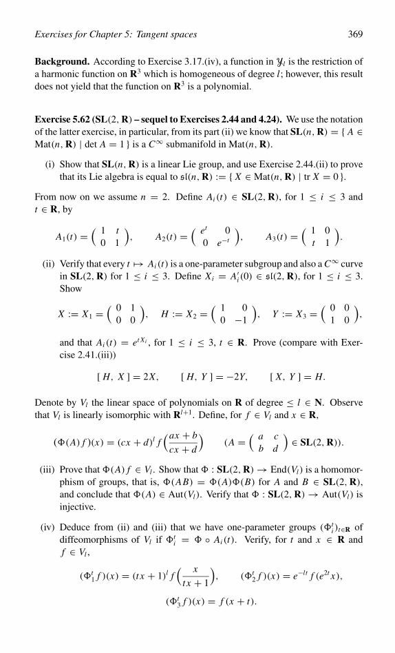
Exercises for Chapter 5: Tangent spaces 369
Background. According to Exercise 3.17.(iv), a function in Yl is the restriction ofa harmonic function on R3 which is homogeneous of degree l; however, this resultdoes not yield that the function on R3 is a polynomial.
Exercise 5.62 (SL(2,R) – sequel to Exercises 2.44 and 4.24). We use the notationof the latter exercise, in particular, from its part (ii) we know that SL(n,R) = { A ∈Mat(n,R) | det A = 1 } is a C∞ submanifold in Mat(n,R).
(i) Show that SL(n,R) is a linear Lie group, and use Exercise 2.44.(ii) to provethat its Lie algebra is equal to sl(n,R) := { X ∈ Mat(n,R) | tr X = 0 }.
From now on we assume n = 2. Define Ai (t) ∈ SL(2,R), for 1 ≤ i ≤ 3 andt ∈ R, by
A1(t) =( 1 t
0 1
), A2(t) =
( et 00 e−t
), A3(t) =
( 1 0t 1
).
(ii) Verify that every t �→ Ai (t) is a one-parameter subgroup and also a C∞ curvein SL(2,R) for 1 ≤ i ≤ 3. Define Xi = A′i (0) ∈ sl(2,R), for 1 ≤ i ≤ 3.Show
X := X1 =( 0 1
0 0
), H := X2 =
( 1 00 −1
), Y := X3 =
( 0 01 0
),
and that Ai (t) = et Xi , for 1 ≤ i ≤ 3, t ∈ R. Prove (compare with Exer-cise 2.41.(iii))
[ H, X ] = 2X, [ H, Y ] = −2Y, [ X, Y ] = H.
Denote by Vl the linear space of polynomials on R of degree ≤ l ∈ N. Observethat Vl is linearly isomorphic with Rl+1. Define, for f ∈ Vl and x ∈ R,
(�(A) f )(x) = (cx + d)l f(ax + b
cx + d
)(A =
( a cb d
)∈ SL(2,R)).
(iii) Prove that �(A) f ∈ Vl . Show that � : SL(2,R)→ End(Vl) is a homomor-phism of groups, that is, �(AB) = �(A)�(B) for A and B ∈ SL(2,R),and conclude that �(A) ∈ Aut(Vl). Verify that � : SL(2,R)→ Aut(Vl) isinjective.
(iv) Deduce from (ii) and (iii) that we have one-parameter groups (�ti )t∈R of
diffeomorphisms of Vl if �ti = � ◦ Ai (t). Verify, for t and x ∈ R and
f ∈ Vl ,
(�t1 f )(x) = (t x + 1)l f
( x
tx + 1
), (�t
2 f )(x) = e−lt f (e2t x),
(�t3 f )(x) = f (x + t).
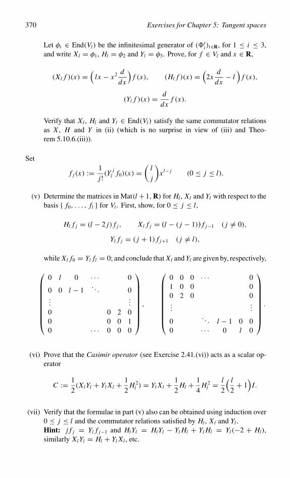
370 Exercises for Chapter 5: Tangent spaces
Let φi ∈ End(Vl) be the infinitesimal generator of (�ti )t∈R, for 1 ≤ i ≤ 3,
and write Xl = φ1, Hl = φ2 and Yl = φ3. Prove, for f ∈ Vl and x ∈ R,
(Xl f )(x) =(
lx − x2 d
dx
)f (x), (Hl f )(x) =
(2x
d
dx− l
)f (x),
(Yl f )(x) = d
dxf (x).
Verify that Xl , Hl and Yl ∈ End(Vl) satisfy the same commutator relationsas X , H and Y in (ii) (which is no surprise in view of (iii) and Theo-rem 5.10.6.(iii)).
Set
f j (x) := 1
j !(Yj
l f0)(x) =(
l
j
)xl− j (0 ≤ j ≤ l).
(v) Determine the matrices in Mat(l+ 1,R) for Hl , Xl and Yl with respect to thebasis { f0, . . . , fl } for Vl . First, show, for 0 ≤ j ≤ l,
Hl f j = (l − 2 j) f j , Xl f j = (l − ( j − 1)) f j−1 ( j = 0),
Yl f j = ( j + 1) f j+1 ( j = l),
while Xl f0 = Yl fl = 0; and conclude that Xl and Yl are given by, respectively,
0 l 0 · · · 0
0 0 l − 1. . . 0
......
0 0 2 00 0 0 10 · · · 0 0 0
,
0 0 0 · · · 01 0 0 00 2 0 0...
...
0. . . l − 1 0 0
0 · · · 0 l 0
.
(vi) Prove that the Casimir operator (see Exercise 2.41.(vi)) acts as a scalar op-erator
C := 1
2(XlYl + Yl Xl + 1
2H 2
l ) = Yl Xl + 1
2Hl + 1
4H 2
l =l
2
( l
2+ 1
)I.
(vii) Verify that the formulae in part (v) also can be obtained using induction over0 ≤ j ≤ l and the commutator relations satisfied by Hl , Xl and Yl .Hint: j f j = Yl f j−1 and HlYl = HlYl − Yl Hl + Yl Hl = Yl(−2 + Hl),similarly XlYl = Hl + Yl Xl , etc.
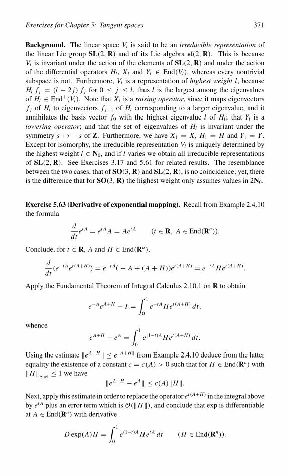
Exercises for Chapter 5: Tangent spaces 371
Background. The linear space Vl is said to be an irreducible representation ofthe linear Lie group SL(2,R) and of its Lie algebra sl(2,R). This is becauseVl is invariant under the action of the elements of SL(2,R) and under the actionof the differential operators Hl , Xl and Yl ∈ End(Vl), whereas every nontrivialsubspace is not. Furthermore, Vl is a representation of highest weight l, becauseHl f j = (l − 2 j) f j for 0 ≤ j ≤ l, thus l is the largest among the eigenvaluesof Hl ∈ End+(Vl). Note that Xl is a raising operator, since it maps eigenvectorsf j of Hl to eigenvectors f j−1 of Hl corresponding to a larger eigenvalue, and itannihilates the basis vector f0 with the highest eigenvalue l of Hl ; that Yl is alowering operator; and that the set of eigenvalues of Hl is invariant under thesymmetry s �→ −s of Z. Furthermore, we have X1 = X , H1 = H and Y1 = Y .Except for isomorphy, the irreducible representation Vl is uniquely determined bythe highest weight l ∈ N0, and if l varies we obtain all irreducible representationsof SL(2,R). See Exercises 3.17 and 5.61 for related results. The resemblancebetween the two cases, that of SO(3,R) and SL(2,R), is no coincidence; yet, thereis the difference that for SO(3,R) the highest weight only assumes values in 2N0.
Exercise 5.63 (Derivative of exponential mapping). Recall from Example 2.4.10the formula
d
dtet A = et A A = Aet A (t ∈ R, A ∈ End(Rn)).
Conclude, for t ∈ R, A and H ∈ End(Rn),
d
dt(e−t Aet (A+H)) = e−t A(− A + (A + H))et (A+H) = e−t A Het (A+H).
Apply the Fundamental Theorem of Integral Calculus 2.10.1 on R to obtain
e−AeA+H − I =∫ 1
0e−t A Het (A+H) dt,
whence
eA+H − eA =∫ 1
0e(1−t)A Het (A+H) dt.
Using the estimate ‖eA+H‖ ≤ e‖A+H‖ from Example 2.4.10 deduce from the latterequality the existence of a constant c = c(A) > 0 such that for H ∈ End(Rn) with‖H‖Eucl ≤ 1 we have
‖eA+H − eA‖ ≤ c(A)‖H‖.Next, apply this estimate in order to replace the operator et (A+H) in the integral aboveby et A plus an error term which is O(‖H‖), and conclude that exp is differentiableat A ∈ End(Rn) with derivative
D exp(A)H =∫ 1
0e(1−t)A Het A dt (H ∈ End(Rn)).
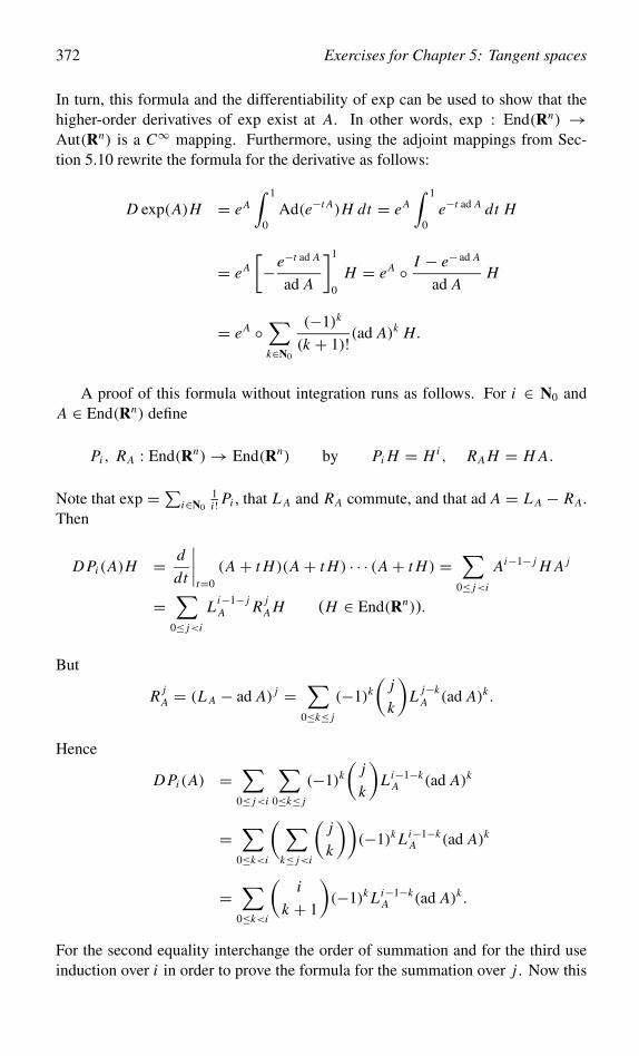
372 Exercises for Chapter 5: Tangent spaces
In turn, this formula and the differentiability of exp can be used to show that thehigher-order derivatives of exp exist at A. In other words, exp : End(Rn) →Aut(Rn) is a C∞ mapping. Furthermore, using the adjoint mappings from Sec-tion 5.10 rewrite the formula for the derivative as follows:
D exp(A)H = eA
∫ 1
0Ad(e−t A)H dt = eA
∫ 1
0e−t ad A dt H
= eA
[−e−t ad A
ad A
]1
0
H = eA ◦ I − e− ad A
ad AH
= eA ◦∑k∈N0
(−1)k
(k + 1)!(ad A)k H.
A proof of this formula without integration runs as follows. For i ∈ N0 andA ∈ End(Rn) define
Pi , RA : End(Rn)→ End(Rn) by Pi H = Hi , RA H = H A.
Note that exp =∑i∈N0
1i ! Pi , that L A and RA commute, and that ad A = L A − RA.
Then
D Pi (A)H = d
dt
∣∣∣∣t=0
(A + t H)(A + t H) · · · (A + t H) =∑
0≤ j<i
Ai−1− j H A j
=∑
0≤ j<i
Li−1− jA R j
A H (H ∈ End(Rn)).
But
R jA = (L A − ad A) j =
∑0≤k≤ j
(−1)k
(j
k
)L j−k
A (ad A)k .
Hence
D Pi (A) =∑
0≤ j<i
∑0≤k≤ j
(−1)k
(j
k
)Li−1−k
A (ad A)k
=∑
0≤k<i
( ∑k≤ j<i
(j
k
))(−1)k Li−1−k
A (ad A)k
=∑
0≤k<i
(i
k + 1
)(−1)k Li−1−k
A (ad A)k .
For the second equality interchange the order of summation and for the third useinduction over i in order to prove the formula for the summation over j . Now this
Exercises for Chapter 5: Tangent spaces 373
implies
D exp(A) =∑i∈N0
1
i !D Pi (A) =∑i∈N0
1
i !∑
0≤k<i
(i
k + 1
)(−1)k Li−1−k
A (ad A)k
=∑i∈N0
∑0≤k<i
(−1)k
(k + 1)!(ad A)k 1
(i − 1− k)! Li−1−kA
=∑k∈N0
(−1)k
(k + 1)!(ad A)k∑
k+1≤i
1
(i − 1− k)!Li−1−kA
= 1− e− ad A
ad A
∑i∈N0
1
i !L Ai = eA ◦ 1− e− ad A
ad A.
Here the fourth equality arises from interchanging the order of summation.
Exercise 5.64 (Closed subgroup is a linear Lie group). In Theorem 5.10.2.(i)we saw that a linear Lie group is a closed subset of GL(n,R). We now prove theconverse statement. Let G ⊂ GL(n,R) be a closed subgroup and define
g = { X ∈ Mat(n,R) | et X ∈ G, for all t ∈ R }.
Then G is a submanifold of Mat(n,R) at I with TI G = g; more precisely, G is alinear Lie group with Lie algebra g.
(i) Use Lie’s product formula from Proposition 5.10.7.(iii) and the closednessof G to show that g is a linear subspace of Mat(n,R).
(ii) Prove that Y ∈ Mat(n,R) belongs to g if there exist sequences (Yk)k∈N inMat(n,R) and (tk)k∈N in R, such that
eYk ∈ G, limk→∞ Yk = 0, lim
k→∞ tkYk = Y.
Hint: Let t ∈ R. For every k ∈ N select mk ∈ Z with |t tk −mk | < 1. Then,if ‖ · ‖ denotes the Euclidean norm on Mat(n,R),
‖mkYk − tY‖ ≤ ‖(mk − t tk)Yk‖ + ‖t tkYk − tY‖ ≤ ‖Yk‖ + |t | ‖tkYk − Y‖.
Further, note emk Yk ∈ G and use that G is closed.
Select a linear subspace h in Mat(n,R) complementary to g, that is, g ⊕ h =Mat(n,R), and define
� : g× h→ GL(n,R) by �(X, Y ) = eX eY .
374 Exercises for Chapter 5: Tangent spaces
(iii) Use the additivity of D�(0, 0) to prove D�(0, 0)(X, Y ) = X + Y , forX ∈ g and Y ∈ h, and deduce that � is a local diffeomorphism onto an openneighborhood of I in GL(n,R).
(iv) Show that exp g is a neighborhood of I in G.Hint: If not, it is possible to choose Xk ∈ g and Yk ∈ h satisfying
eXk eYk ∈ G, Yk = 0, limk→∞(Xk, Yk) = (0, 0).
Prove eYk ∈ G. Next, consider Yk = 1‖Yk‖Yk . By compactness of the unit
sphere in Mat(n,R) and by going over to a subsequence we may assumethat there is Y ∈ Mat(n,R) with limk→∞ Yk = Y . Hence we have obtainedsequences (Yk)k∈N in h and ( 1
‖Yk‖)k∈N in R, such that
eYk ∈ G, limk→∞Yk = 0, lim
k→∞1
‖Yk‖Yk = Y ∈ h.
From part (ii) obtain Y ∈ g and conclude Y = 0, which is a contradiction.
(v) Deduce from part (iv) that G is a linear Lie group.
Exercise 5.65 (Reflections, rotations and Hamilton’s Theorem – sequel to Ex-ercises 2.5, 4.22, 5.26 and 5.27 – needed for Exercises 5.66, 5.67 and 5.72).For
p = (p0, p) ∈ S3 = { (p0, p) ∈ R × R3 � R4 | p20 + ‖p‖2 = 1 }
we define
R p ∈ End(R3) by R p x = 2〈p, x〉 p + (p20 − ‖p‖2) x + 2p0 p × x .
Note that R p = R− p, so we may assume p0 ≥ 0.
(i) Suppose p0 = 0. Show −R p is the reflection of R3 in the two-dimensionallinear subspace Np = { x ∈ R3 | 〈x, p〉 = 0 }.
Verify that R p ∈ SO(R3) in the following two ways. Conversely, prove that everyelement in SO(R3) is of the form R p for some p ∈ S3.
(ii) Note that (p20 −‖p‖2)2+ (2p0‖p‖)2 = 1. Therefore we can find 0 ≤ α ≤ π
such that p20 − ‖p‖2 = cosα and 2p0‖p‖ = sin α. Hence there is a ∈ S2
with p = sin α2 a and thus p0 = cos α
2 , which implies that R p takes the formas in Euler’s formula in Exercise 4.22 or 5.58.
(iii) Use the results of Exercise 5.26 to show that R p preserves the norm, andtherefore the inner product on R3, and using that p �→ det R p is a continuousmapping from the connected space S3 to {±1} (see Lemma 1.9.3) provedet R p = 1.
Exercises for Chapter 5: Tangent spaces 375
(iv) Verify that we get the following rational parametrization of a matrix inSO(3,R):
R p = (p20 − ‖p‖2)I + 2(ppt + p0rp).
We now study relations between reflections and rotations in R3.
(v) Let Si be the reflection of R3 in the two-dimensional linear subspace Ni ⊂ R3
for 1 ≤ i ≤ 2. If α is the angle between N1 and N2 measured from N1 to N2,then S2S1 (note the ordering) is the rotation of R3 about the axis N1 ∩ N2 bythe angle 2α. Prove this. Conversely, use Euler’s Theorem in Exercise 2.5 toprove that every element in SO(R3) is the product of two reflections of R3.Hint: It is sufficient to verify the result for the reflections S1 and S2 of R2 inthe one-dimensional linear subspace Re1 and R(cosα, sin α), respectively,satisfying, with x ∈ R2,
S1 x =( x1
−x2
), S2 x = x + 2(x1 sin α − x2 cosα)
( − sin αcosα
).
Let �(A) be a spherical triangle as in Exercise 5.27 determined by ai ∈ S2 andwith angles αi , and denote by Si the reflection of R3 in the two-dimensional linearsubspace containing ai+1 and ai+2 for 1 ≤ i ≤ 3.
(vi) By means of (v) prove that Si+1Si+2 = R2αi ,ai , the rotation of R3 about theaxis ai and by the angle 2αi for 1 ≤ i ≤ 3. Using S2
i = I deduce Hamilton’sTheorem
R2α1,a1 R2α2,a2 R2α3,a3 = I.
Note that this is an analog of the fact that the sum of double the angles in aplanar triangle equals 2π .
Exercise 5.66 (Reflections, rotations, Cayley–Klein parameters and Sylvester’sTheorem – sequel to Exercises 5.26, 5.27 and 5.65 – needed for Exercises 5.67,5.68, 5.69 and 5.72). Let 0 ≤ α1 ≤ π and a1 ∈ S2. According to Exercise 5.65.(v)the rotation Rα1,a1 of R3 by the angle α1 about the axis Ra1 is the composition S2S1
of reflections Si in two-dimensional linear subspaces Ni , for 1 ≤ i ≤ 2, of R3 thatintersect in Ra1 and make an angle of α1
2 . We will prove that any such pair (S1, S2)
or configuration (N1, N2) is determined by the parameter ± p of Rα1,a1 given by
p = (p0, p) =(
cosα1
2, sin
α1
2a1
)∈ S3 = { (p0, p) ∈ R×R3 | p2
0+‖p‖2 = 1 }.
Further, composition of rotations corresponds to the composition of parametersdefined in (�) below.
(i) Set Np = { x ∈ R3 | 〈x, p〉 = 0 }. Define
ρ p ∈ End(Np) by ρ p x = p0x + p × x .
376 Exercises for Chapter 5: Tangent spaces
Show that ρ p = ρ− p is the counterclockwise (measured with respect to p)rotation in Np by the angle α1
2 , and furthermore, that Rα1,a1 is the compositionS2S1 of reflections S1 and S2 in the two-dimensional linear subspaces N1 andN2 spanned by p and x , and p and ρ p x , respectively.
(ii) Now suppose Rα2,a2 is a second rotation with corresponding parameter ±qgiven by q = (q0, q) = (cos α2
2 , sin α22 a2) ∈ S3. Consider the triple of
vectors in S2
x1 := ρ−1p x2 ∈ Np, x2 := 1
‖q × p‖ q × p ∈ Np ∩ Nq,
x3 := ρq x2 ∈ Nq .
Then x1 and x2, and x2 and x3, determine a decomposition of Rα1,a1 and Rα2,a2
in reflections in two-dimensional linear subspaces N1 and N2, and N3 andN4, respectively, where N2 ∩ N3 = R(q × p). In particular,
x2 = ρ p x1 = p0x1 + p × x1, x3 = ρq x2 = q0x2 + q × x2.
Eliminate x2 from these equations to find
x3 = (q0 p0 − 〈q, p〉)x1 + (q0 p + p0q + q × p)× x1 =: r0x1 + r × x1.
Using Exercise 5.26.(i) show that r = (r0, r) ∈ S3. Prove that x1 and x3 ∈ Nr .
We have found the following rule of composition for the parameters of rotations:
(�) q· p = (q0, q)·(p0, p) = (q0 p0−〈q, p〉, q0 p+p0q+q×p) =: (r0, r) = r.
Next we want to prove that the composite parameter ±r is the parameter of thecomposition Rα3,a3 = Rα2,a2 Rα1,a1 .
(iii) Let 0 ≤ α3 ≤ π and a3 ∈ S2 be determined by r , thus (cos α32 , sin α3
2 a3) =(r0, r). Then �(x1, x2, x3) is the spherical triangle with sides α2
2 , α32 and α1
2 ,see Exercise 5.27. The polar triangle �′(x1, x2, x3) has vertices a2, −a3 anda1, and angles 2π−α2
2 , 2π−α32 and 2π−α1
2 . Apply Hamilton’s Theorem fromExercise 5.65.(vi) to this polar triangle to find
R2π−α2,a2 Rα3,a3 R2π−α1,a1 = I, thus Rα3,a3 = Rα2,a2 Rα1,a1 .
Note that the results in (ii) and (iii) give a geometric construction for the compositionof two rotations, which is called Sylvester’s Theorem; see Exercise 5.67.(xii) for adifferent construction.
The Cayley–Klein parameter of the rotation Rα,a is the pair of matrices ± p ∈Mat(2,C) given by the following formula, where i = √−1,
p =( p0 + i p3 −p2 + i p1
p2 + i p1 p0 − i p3
)=
cosα
2+ ia3 sin
α
2(−a2 + ia1) sin
α
2
(a2 + ia1) sinα
2cos
α
2− ia3 sin
α
2
.
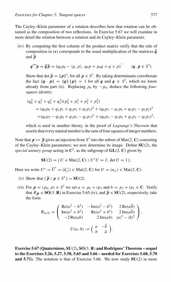
Exercises for Chapter 5: Tangent spaces 377
The Cayley–Klein parameter of a rotation describes how that rotation can be ob-tained as the composition of two reflections. In Exercise 5.67 we will examine inmore detail the relation between a rotation and its Cayley–Klein parameter.
(iv) By computing the first column of the product matrix verify that the rule ofcomposition in (�) corresponds to the usual multiplication of the matrices qand p
q · p = q p = (q0 p0 − 〈q, p〉, q0 p + p0q + q × p) (q, p ∈ S3).
Show that det p = ‖ p‖2, for all p ∈ S3. By taking determinants corroboratethe fact ‖q · p‖ = ‖q‖ ‖ p‖ = 1 for all q and q ∈ S3, which we knowalready from part (ii). Replacing p0 by −p0, deduce the following four-square identity:
(q20 + q2
1 + q22 + q2
3 )(p20 + p2
1 + p22 + p2
3)
= (q0 p0 + q1 p1 + q2 p2 + q3 p3)2 + (q0 p1 − q1 p0 + q2 p3 − q3 p2)
2
+(q0 p2 − q2 p0 + q3 p1 − q1 p3)2 + (q0 p3 − q3 p0 + q1 p2 − q2 p1)
2,
which is used in number theory, in the proof of Lagrange’s Theorem thatasserts that every natural number is the sum of four squares of integer numbers.
Note that p �→ p gives an injection from S3 into the subset of Mat(2,C) consistingof the Cayley–Klein parameters; we now determine its image. Define SU(2), thespecial unitary group acting in C2, as the subgroup of GL(2,C) given by
SU(2) = {U ∈ Mat(2,C) | U ∗U = I, det U = 1 }.Here we write U ∗ = U
t = (u ji ) ∈ Mat(2,C) for U = (ui j ) ∈ Mat(2,C).
(v) Show that { p | p ∈ S3 } = SU(2).
(vi) For p = (p0, p) ∈ S3 we set a = p0 + i p3 and b = p2 + i p1 ∈ C. Verifythat R p ∈ SO(3,R) in Exercise 5.65.(iv), and p ∈ SU(2), respectively, takethe form
R(a,b) = Re(a2 − b2) − Im(a2 − b2) 2 Re(ab)
Im(a2 + b2) Re(a2 + b2) 2 Im(ab)−2 Re(ab) 2 Im(ab) |a|2 − |b|2
,
U (a, b) :=( a −b
b a
).
Exercise 5.67 (Quaternions, SU(2), SO(3,R) and Rodrigues’ Theorem – sequelto the Exercises 5.26, 5.27, 5.58, 5.65 and 5.66 – needed for Exercises 5.68, 5.70and 5.71). The notation is that of Exercise 5.66. We now study SU(2) in more
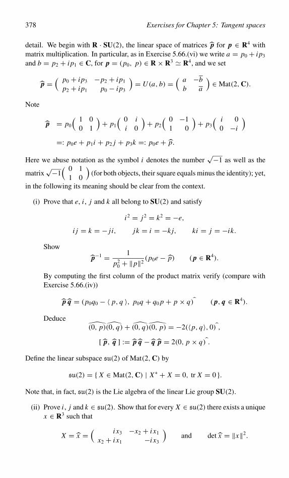
378 Exercises for Chapter 5: Tangent spaces
detail. We begin with R · SU(2), the linear space of matrices p for p ∈ R4 withmatrix multiplication. In particular, as in Exercise 5.66.(vi) we write a = p0 + i p3
and b = p2 + i p1 ∈ C, for p = (p0, p) ∈ R × R3 � R4, and we set
p =( p0 + i p3 −p2 + i p1
p2 + i p1 p0 − i p3
)= U (a, b) =
( a −bb a
)∈ Mat(2,C).
Note
p = p0
( 1 00 1
)+ p1
( 0 ii 0
)+ p2
( 0 −11 0
)+ p3
( i 00 −i
)=: p0e + p1i + p2 j + p3k =: p0e + p.
Here we abuse notation as the symbol i denotes the number√−1 as well as the
matrix√−1
( 0 11 0
)(for both objects, their square equals minus the identity); yet,
in the following its meaning should be clear from the context.
(i) Prove that e, i , j and k all belong to SU(2) and satisfy
i2 = j2 = k2 = −e,
i j = k = − j i, jk = i = −k j, ki = j = −ik.
Show
p−1 = 1
p20 + ‖p‖2
(p0e − p) ( p ∈ R4).
By computing the first column of the product matrix verify (compare withExercise 5.66.(iv))
p q = (p0q0 − 〈 p, q 〉, p0q + q0 p + p × q ) ( p, q ∈ R4).
Deduce(0, p)(0, q)+ (0, q)(0, p) = −2(〈p, q〉, 0) ,
[ p, q ] := p q − q p = 2(0, p × q ) .
Define the linear subspace su(2) of Mat(2,C) by
su(2) = { X ∈ Mat(2,C) | X∗ + X = 0, tr X = 0 }.Note that, in fact, su(2) is the Lie algebra of the linear Lie group SU(2).
(ii) Prove i , j and k ∈ su(2). Show that for every X ∈ su(2) there exists a uniquex ∈ R3 such that
X = x =( i x3 −x2 + i x1
x2 + i x1 −i x3
)and det x = ‖x‖2.
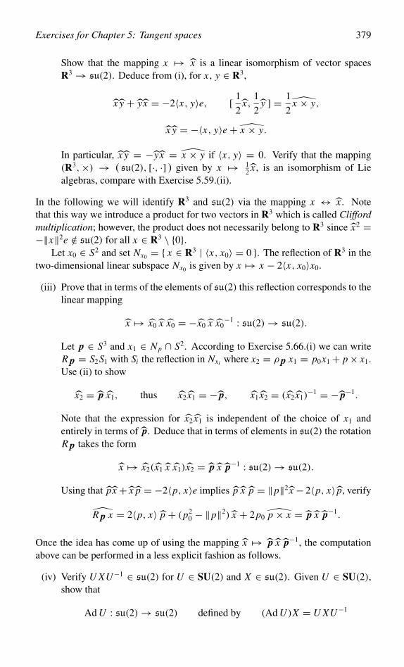
Exercises for Chapter 5: Tangent spaces 379
Show that the mapping x �→ x is a linear isomorphism of vector spacesR3 → su(2). Deduce from (i), for x , y ∈ R3,
x y + y x = −2〈x, y〉e, [ 1
2x,
1
2y ] = 1
2x × y,
x y = −〈x, y〉e + x × y.
In particular, x y = −y x = x × y if 〈x, y〉 = 0. Verify that the mapping(R3,×) → ( su(2), [·, ·] ) given by x �→ 1
2 x , is an isomorphism of Liealgebras, compare with Exercise 5.59.(ii).
In the following we will identify R3 and su(2) via the mapping x ↔ x . Notethat this way we introduce a product for two vectors in R3 which is called Cliffordmultiplication; however, the product does not necessarily belong to R3 since x2 =−‖x‖2e /∈ su(2) for all x ∈ R3 \ {0}.
Let x0 ∈ S2 and set Nx0 = { x ∈ R3 | 〈x, x0〉 = 0 }. The reflection of R3 in thetwo-dimensional linear subspace Nx0 is given by x �→ x − 2〈x, x0〉x0.
(iii) Prove that in terms of the elements of su(2) this reflection corresponds to thelinear mapping
x �→ x0 x x0 = −x0 x x0−1 : su(2)→ su(2).
Let p ∈ S3 and x1 ∈ Np ∩ S2. According to Exercise 5.66.(i) we can writeR p = S2S1 with Si the reflection in Nxi where x2 = ρ p x1 = p0x1+ p× x1.Use (ii) to show
x2 = p x1, thus x2 x1 = − p, x1 x2 = (x2 x1)−1 = − p−1.
Note that the expression for x2 x1 is independent of the choice of x1 andentirely in terms of p. Deduce that in terms of elements in su(2) the rotationR p takes the form
x �→ x2(x1 x x1)x2 = p x p−1 : su(2)→ su(2).
Using that px + x p = −2〈p, x〉e implies p x p = ‖p‖2 x − 2〈p, x〉 p, verify
R p x = 2〈p, x〉 p + (p20 − ‖p‖2) x + 2p0 p × x = p x p−1.
Once the idea has come up of using the mapping x �→ p x p−1, the computationabove can be performed in a less explicit fashion as follows.
(iv) Verify U XU−1 ∈ su(2) for U ∈ SU(2) and X ∈ su(2). Given U ∈ SU(2),show that
Ad U : su(2)→ su(2) defined by (Ad U )X = U XU−1
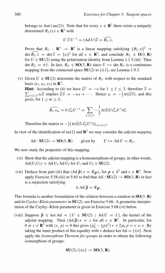
380 Exercises for Chapter 5: Tangent spaces
belongs to Aut ( su(2)). Note that for every x ∈ R3 there exists a uniquelydetermined RU (x) ∈ R3 with
U x U−1 = (Ad U )x = RU x .
Prove that RU : R3 → R3 is a linear mapping satisfying ‖RU x‖2 =det RU x = det x = ‖x‖2 for all x ∈ R3, and conclude RU ∈ O(3,R)for U ∈ SU(2) using the polarization identity from Lemma 1.1.5.(iii). Thusdet RU = ±1. In fact, RU ∈ SO(3,R) since U �→ det RU is a continuousmapping from the connected space SU(2) to {±1}, see Lemma 1.9.3.
(v) Given U ∈ SU(2) determine the matrix of RU with respect to the standardbasis (e1, e2, e3) in R3.Hint: According to (ii) we have el
2 = −e for 1 ≤ l ≤ 3, therefore x =∑1≤l≤3 xl el implies el x = −xle + · · · . Hence xl = − 1
2 tr(el x), and thisgives, for 1 ≤ m ≤ 3,
RU em = UemU−1 =∑
1≤l≤3
−1
2tr(elU emU ∗)el .
Therefore the matrix is − 12 ( tr(elU emU ∗))1≤l,m≤3.
In view of the identification of su(2) and R3 we may consider the adjoint mapping
Ad : SU(2)→ SO(3,R) given by U �→ Ad U = RU .
We now study the properties of this mapping.
(vi) Show that the adjoint mapping is a homomorphism of groups, in other words,Ad(U1U2) = Ad U1 Ad U2 for U1 and U2 ∈ SU(2).
(vii) Deduce from part (iii) that (Ad p) x = R px , for p ∈ S3 and x ∈ R3. Nowapply Exercise 5.58.(iii) or 5.65 to find that Ad : SU(2)→ SO(3,R) in factis a surjection satisfying
±Ad p = R p.
This formula is another formulation of the relation between a rotation in SO(3,R)and its Cayley–Klein parameter in SU(2), see Exercise 5.66. A geometric interpre-tation of the Cayley–Klein parameter is given in Exercise 5.68.(vi) below.
(viii) Suppose p ∈ ker Ad = {U ∈ SU(2) | Ad U = I }, the kernel of theadjoint mapping. Then (Ad p) x = x for all x ∈ R3. In particular, for0 = x ∈ R3 with 〈x, p〉 = 0 this gives (p2
0 − ‖p‖2) x + 2p0 p × x = x . Bytaking the inner product of this equality with x deduce ker Ad = {±e}. Nextapply the Isomorphism Theorem for groups in order to obtain the followingisomorphism of groups:
SU(2)/{±e} → SO(3,R).
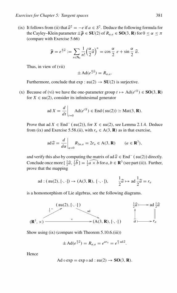
Exercises for Chapter 5: Tangent spaces 381
(ix) It follows from (ii) that a2 = −e if a ∈ S2. Deduce the following formula forthe Cayley–Klein parameter± p ∈ SU(2) of Rα,a ∈ SO(3,R) for 0 ≤ α ≤ π
(compare with Exercise 5.66)
p = eα2 a :=
∑n∈N0
1
n!(α
2a)n = cos
α
2e + sin
α
2a.
Thus, in view of (vii)
±Ad(eα2 a) = Rα,a.
Furthermore, conclude that exp : su(2)→ SU(2) is surjective.
(x) Because of (vi) we have the one-parameter group t �→ Ad(et X ) ∈ SO(3,R)for X ∈ su(2), consider its infinitesimal generator
ad X = d
dt
∣∣∣∣t=0
Ad(et X ) ∈ End ( su(2)) � Mat(3,R).
Prove that ad X ∈ End− ( su(2)), for X ∈ su(2), see Lemma 2.1.4. Deducefrom (ix) and Exercise 5.58.(ii), with ra ∈ A(3,R) as in that exercise,
ad a = d
dα
∣∣∣∣α=0
R2α,a = 2ra ∈ A(3,R) (a ∈ R3),
and verify this also by computing the matrix of ad a ∈ End− ( su(2)) directly.Conclude once more [ 1
2 a, 12 b ] = 1
2 a × b for a, b ∈ R3 (see part (ii)). Further,prove that the mapping
ad : ( su(2), [·, ·]) → (A(3,R), [ ·, · ]), 1
2a �→ ad
1
2a = ra
is a homomorphism of Lie algebras, see the following diagrams.
( su(2), [·, ·] )ad
���������������
(R3,×) × ��
12 �������������
(A(3,R), [·, ·] )
12 a � �� ad 1
2 a
a�
��
� �� ra
Show using (ix) (compare with Theorem 5.10.6.(iii))
±Ad(eα2 a) = Rα,a = eαra = e
α2 ad a.
Hence
Ad ◦ exp = exp ◦ ad : su(2)→ SO(3,R).
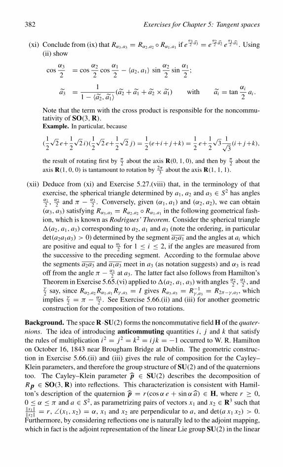
382 Exercises for Chapter 5: Tangent spaces
(xi) Conclude from (ix) that Rα3,a3 = Rα2,a2 ◦ Rα1,a1 if eα32 a3 = e
α22 a2 e
α12 a1 . Using
(ii) show
cosα3
2= cos
α2
2cos
α1
2− 〈a2, a1〉 sin
α2
2sin
α1
2;
a3 = 1
1− 〈a2, a1〉(a2 + a1 + a2 × a1) with ai = tanαi
2ai .
Note that the term with the cross product is responsible for the noncommu-tativity of SO(3,R).Example. In particular, because
(1
2
√2 e+ 1
2
√2 i)(
1
2
√2 e+ 1
2
√2 j) = 1
2(e+i+ j+k) = 1
2e+ 1
2
√3
1√3(i+ j+k),
the result of rotating first by π2 about the axis R(0, 1, 0), and then by π
2 about theaxis R(1, 0, 0) is tantamount to rotation by 2π
3 about the axis R(1, 1, 1).
(xii) Deduce from (xi) and Exercise 5.27.(viii) that, in the terminology of thatexercise, the spherical triangle determined by a1, a2 and a3 ∈ S2 has anglesα12 , α2
2 and π − α32 . Conversely, given (α1, a1) and (α2, a2), we can obtain
(α3, a3) satisfying Rα3,a3 = Rα2,a2 ◦ Rα1,a1 in the following geometrical fash-ion, which is known as Rodrigues’ Theorem. Consider the spherical triangle�(a2, a1, a3) corresponding to a2, a1 and a3 (note the ordering, in particulardet(a2a1a3) > 0) determined by the segment a2a1 and the angles at ai whichare positive and equal to αi
2 for 1 ≤ i ≤ 2, if the angles are measured fromthe successive to the preceding segment. According to the formulae abovethe segments a2a3 and a1a3 meet in a3 (as notation suggests) and α3 is readoff from the angle π − α3
2 at a3. The latter fact also follows from Hamilton’sTheorem in Exercise 5.65.(vi) applied to�(a2, a1, a3)with angles α2
2 , α12 , and
γ
2 say, since Rα2,a2 Rα1,a1 Rγ,a3 = I gives Rα3,a3 = R−1γ,a3
= R2π−γ,a3 , whichimplies γ
2 = π − α32 . See Exercise 5.66.(ii) and (iii) for another geometric
construction for the composition of two rotations.
Background. The space R ·SU(2) forms the noncommutative field H of the quater-nions. The idea of introducing anticommuting quantities i , j and k that satisfythe rules of multiplication i2 = j2 = k2 = i jk = −1 occurred to W. R. Hamiltonon October 16, 1843 near Brougham Bridge at Dublin. The geometric construc-tion in Exercise 5.66.(ii) and (iii) gives the rule of composition for the Cayley–Klein parameters, and therefore the group structure of SU(2) and of the quaternionstoo. The Cayley–Klein parameter p ∈ SU(2) describes the decomposition ofR p ∈ SO(3,R) into reflections. This characterization is consistent with Hamil-ton’s description of the quaternion p = r(cosα e + sin α a) ∈ H, where r ≥ 0,0 ≤ α ≤ π and a ∈ S2, as parametrizing pairs of vectors x1 and x2 ∈ R3 such that‖x1‖‖x2‖ = r , ∠(x1, x2) = α, x1 and x2 are perpendicular to a, and det(a x1 x2) > 0.Furthermore, by considering reflections one is naturally led to the adjoint mapping,which in fact is the adjoint representation of the linear Lie group SU(2) in the linear
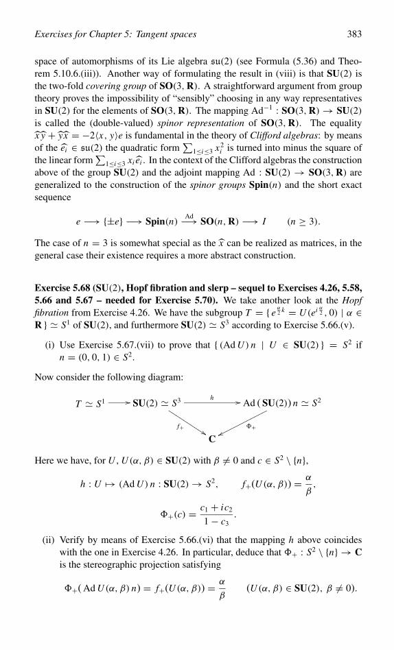
Exercises for Chapter 5: Tangent spaces 383
space of automorphisms of its Lie algebra su(2) (see Formula (5.36) and Theo-rem 5.10.6.(iii)). Another way of formulating the result in (viii) is that SU(2) isthe two-fold covering group of SO(3,R). A straightforward argument from grouptheory proves the impossibility of “sensibly” choosing in any way representativesin SU(2) for the elements of SO(3,R). The mapping Ad−1 : SO(3,R)→ SU(2)is called the (double-valued) spinor representation of SO(3,R). The equalityx y + y x = −2〈x, y〉e is fundamental in the theory of Clifford algebras: by meansof the ei ∈ su(2) the quadratic form
∑1≤i≤3 x2
i is turned into minus the square ofthe linear form
∑1≤i≤3 xi ei . In the context of the Clifford algebras the construction
above of the group SU(2) and the adjoint mapping Ad : SU(2) → SO(3,R) aregeneralized to the construction of the spinor groups Spin(n) and the short exactsequence
e −→ {±e} −→ Spin(n)Ad−→ SO(n,R) −→ I (n ≥ 3).
The case of n = 3 is somewhat special as the x can be realized as matrices, in thegeneral case their existence requires a more abstract construction.
Exercise 5.68 (SU(2), Hopf fibration and slerp – sequel to Exercises 4.26, 5.58,5.66 and 5.67 – needed for Exercise 5.70). We take another look at the Hopffibration from Exercise 4.26. We have the subgroup T = { e
α2 k = U (ei α2 , 0) | α ∈
R } � S1 of SU(2), and furthermore SU(2) � S3 according to Exercise 5.66.(v).
(i) Use Exercise 5.67.(vii) to prove that { (Ad U ) n | U ∈ SU(2) } = S2 ifn = (0, 0, 1) ∈ S2.
Now consider the following diagram:
T � S1 �� SU(2) � S3 h ��
f+������������ Ad ( SU(2)) n � S2
�+��������������
C
Here we have, for U , U (α, β) ∈ SU(2) with β = 0 and c ∈ S2 \ {n},
h : U �→ (Ad U ) n : SU(2)→ S2, f+(U (α, β)) = α
β,
�+(c) = c1 + ic2
1− c3.
(ii) Verify by means of Exercise 5.66.(vi) that the mapping h above coincideswith the one in Exercise 4.26. In particular, deduce that �+ : S2 \ {n} → Cis the stereographic projection satisfying
�+( Ad U (α, β) n) = f+(U (α, β)) = α
β(U (α, β) ∈ SU(2), β = 0).
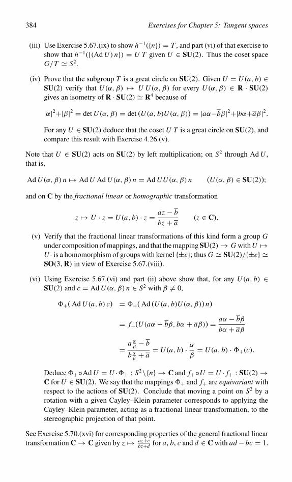
384 Exercises for Chapter 5: Tangent spaces
(iii) Use Exercise 5.67.(ix) to show h−1({n}) = T , and part (vi) of that exercise toshow that h−1({(Ad U ) n}) = U T given U ∈ SU(2). Thus the coset spaceG/T � S2.
(iv) Prove that the subgroup T is a great circle on SU(2). Given U = U (a, b) ∈SU(2) verify that U (α, β) �→ U U (α, β) for every U (α, β) ∈ R · SU(2)gives an isometry of R · SU(2) � R4 because of
|α|2+|β|2 = det U (α, β) = det (U (a, b)U (α, β)) = |aα−bβ|2+|bα+aβ|2.For any U ∈ SU(2) deduce that the coset U T is a great circle on SU(2), andcompare this result with Exercise 4.26.(v).
Note that U ∈ SU(2) acts on SU(2) by left multiplication; on S2 through Ad U ,that is,
Ad U (α, β) n �→ Ad U Ad U (α, β) n = Ad UU (α, β) n (U (α, β) ∈ SU(2));and on C by the fractional linear or homographic transformation
z �→ U · z = U (a, b) · z = az − b
bz + a(z ∈ C).
(v) Verify that the fractional linear transformations of this kind form a group Gunder composition of mappings, and that the mapping SU(2)→ G with U �→U · is a homomorphism of groups with kernel {±e}; thus G � SU(2)/{±e} �SO(3,R) in view of Exercise 5.67.(viii).
(vi) Using Exercise 5.67.(vi) and part (ii) above show that, for any U (a, b) ∈SU(2) and c = Ad U (α, β) n ∈ S2 with β = 0,
�+( Ad U (a, b) c) = �+( Ad (U (a, b)U (α, β)) n)
= f+(U (aα − bβ, bα + aβ)) = aα − bβ
bα + aβ
= a αβ− b
b αβ+ a
= U (a, b) · αβ= U (a, b) ·�+(c).
Deduce�+◦Ad U = U ·�+ : S2\{n} → C and f+◦U = U · f+ : SU(2)→C for U ∈ SU(2). We say that the mappings�+ and f+ are equivariant withrespect to the actions of SU(2). Conclude that moving a point on S2 by arotation with a given Cayley–Klein parameter corresponds to applying theCayley–Klein parameter, acting as a fractional linear transformation, to thestereographic projection of that point.
See Exercise 5.70.(xvi) for corresponding properties of the general fractional lineartransformation C → C given by z �→ az+c
bz+d for a, b, c and d ∈ C with ad− bc = 1.
Exercises for Chapter 5: Tangent spaces 385
(vii) Let U1 and U2 ∈ SU(2) � S3 ⊂ R4 and suppose 〈U1,U2〉 = 12 tr(U1U ∗
2 ) =cos θ . Consider U ∈ SU(2) belonging to the great circle in SU(2) connectingU1 and U2. Because U lies in the plane in R4 spanned by U1 and U2, thereexist λ and µ ∈ R satisfying U = λU1 + µU2 and ‖λU1 + µU2‖ = 1.Writing 〈U,U1〉 = cos tθ , for suitable t ∈ [ 0, 1 ], deduce
U = U (t) = sin(1− t)θ
sin θU1 + sin tθ
sin θU2.
In computer graphics the curve [ 0, 1 ] → SU(2) with t �→ U (t) is known asthe slerp (= spherical linear interpolation) between U1 and U2; the correspondingrotations interpolate smoothly between the rotations with Cayley-Klein parameterU1 and U2, respectively.
Exercise 5.69 (Cartan decomposition of SL(2,C) – sequel to Exercises 2.44and 5.66 – needed for Exercises 5.70 and 5.71). Let SU(2) and su(2) be as inExercise 5.67. Set SL(2,C) = { A ∈ GL(2,C) | det A = 1 } and
sl(2,C) = { X ∈ Mat(2,C) | tr X = 0 }, p = i su(2) = sl(2,C) ∩ H(2,C).
Here H(2,C) = { A ∈ Mat(2,C) | A∗ = A } where A∗ = At
as usual denotes thelinear subspace of Hermitian matrices. Note that sl(2,C) = su(2) ⊕ p as linearspaces over R.
(i) For every A ∈ SL(2,C) there exist U ∈ SU(2) and X ∈ p such that thefollowing Cartan decomposition holds:
A = U eX .
Indeed, write D(a, b) for the diagonal matrix in Mat(2,C) with coefficientsa and b ∈ C. Since A∗A ∈ H(2,C) is positive–definite, by the versionover C of the Spectral Theorem 2.9.3 there exist V ∈ SU(2) and λ > 0with A∗A = V D(λ, λ−1)V−1. Now D(λ, λ−1) = exp 2D(µ,−µ) withµ = 1
2 log λ ∈ R. Set
X = V D(µ,−µ)V−1 ∈ p, U = A e−X ,
and verify U ∈ SU(2).
(ii) Verify that eX ∈ SL(2,C) ∩ H(2,C) is positive definite for X ∈ p, andconversely, that every positive definite Hermitian element in SL(2,C) is ofthis form, for a suitable X ∈ p (see Exercise 2.44.(ii)).
(iii) Define π : SU(2) × p → SL(2,C) by π(U, X) = U eX . Show that πis continuous and deduce from Exercise 5.66.(v) and Theorem 1.9.4 thatSL(2,C) is a connected set.
386 Exercises for Chapter 5: Tangent spaces
(iv) Verify that SL(2,C)∩H(2,C) is not a subgroup of SL(2,C) by considering
the product of( 2 −i
i 1
)and
( 1 11 2
).
Background. The Cartan decomposition is a version over C of the polar decompo-sition of an automorphism from Exercise 2.68. Moreover, it is the global version ofthe decomposition (at the infinitesimal level) of an arbitrary matrix into Hermitianand anti-Hermitian matrices, the complex analog of the Stokes decomposition fromDefinition 8.1.4.
Exercise 5.70 (Hopf fibration, SL(2,C) and Lorentz group – sequel to Exercises4.26, 5.67, 5.68, 5.69 and 8.32 – needed for Exercise 5.71). Important properties ofthe Lorentz group Lo(4,R) from Exercise 8.32 can be obtained using an extension ofthe Hopf mapping from Exercise 4.26. In this fashion SL(2,C) = { A ∈ GL(2,C) |det A = 1 } arises naturally as the two-fold covering group of the proper Lorentzgroup Lo◦(4,R) which is defined as follows. We denote by C the (light) cone inR4, and by C+ the forward (light) cone, respectively, given by
C = { (x0, x) ∈ R4 | x20 = ‖x‖2 }, C+ = { (x0, x) ∈ C | x0 ≥ 0 }.
Note that any L ∈ Lo(4,R) preserves C , i.e., satisfies L(C) ⊂ C (and thereforeL(C) = C). We define Lo◦(4,R), the proper Lorentz group, to be the subgroupof Lo(4,R) consisting of elements preserving C+ and having determinant equal to1. Elements of Lo◦(4,R) are said to be proper Lorentz transformations. In thisexercise we identify linear transformations and matrices using the standard basis inR4.
We begin by introducing the Hopf mapping in a natural way. To this end, setH(2,C) = { A ∈ Mat(2,C) | A∗ = A } where A∗ = A
tas usual, and define
κ : C2 → H(2,C) byκ(z) = 2 z z∗ (z ∈ C2),
in other words
κ( a
b
)= 2
( aa abba bb
)(a, b ∈ C).
Note that κ is neither injective nor surjective.
(i) Verify det κ(z) = 0 and κ ◦ A(z) = A κ(z) A∗ for z ∈ C2 and A ∈ Mat(2,C).
Define for all x = (x0, x) ∈ R×R3 � R4 (see Exercise 5.67.(ii) for the definitionof x ∈ su(2))
x = x0e − i x =( x0 + x3 x1 + i x2
x1 − i x2 x0 − x3
)∈ H(2,C).
Exercises for Chapter 5: Tangent spaces 387
(ii) Show that the mapping x �→ x is a linear isomorphism of vector spacesR4 → H(2,C); and denote its inverse by ι : H(2,C)→ R4. Prove
det x = x20 − ‖x‖2 =: (x)2, tr x = 2x0 (x ∈ R4).
(iii) Prove that h := ι ◦ κ : C2 → R4 is given by (compare with Exercise 4.26)
h( a
b
)=
|a|2 + |b|22 Re(ab)2 Im(ab)|a|2 − |b|2
(a, b ∈ C).
Deduce from (i) that (h ◦ A(z)) = A κ(z) A∗ for A ∈ Mat(2,C) and z ∈ C2.Further show that h(λz) = |λ|2h(z), for all λ ∈ C and z ∈ C2.
(iv) Using (ii) show det κ(z) = (h(z))2 and using (i) deduce h(z) ∈ C+ for allz ∈ C2. More precisely, prove that h : C2 → C+ is surjective, and that
h−1({h(z)}) = { eiαz | α ∈ R } (z ∈ C2).
Compare this result with the Exercises 4.26 and 5.68.(iii).
Next we show that the natural action of A ∈ SL(2,C) on C2 induces a Lorentztransformation L A ∈ Lo◦(4,R) of R4.
(v) Since h ◦ A : C2 → C+ for all A ∈ Mat(2,C), and h ◦ A ◦ eiα = h ◦ A forall α ∈ R, we have the well-defined mapping
L A : C+ → C+ given by L A ◦ h = h ◦ A : C2 → C+.
Deduce from (iii) that (L A ◦ h(z)) = A κ(z) A∗. Given x ∈ C+, part (iv)now implies that we can find z ∈ C2 with h(z) = x, and thus κ(z) = x. Thisgives
L A(x) = A x A∗ (x ∈ C+).
C+ spans all of R4 as the linearly independent vectors e0 + e1, e0 + e2 ande0 ± e3 in R4 all belong to C+. Therefore the mapping L A in fact is therestriction to C+ of a unique linear mapping, also denoted by L A,
L A ∈ End(R4) satisfying L A x = A x A∗ (x ∈ R4).
Using (ii) prove
(L A x)2 = det(A x A∗) = det x = (x)2 (A ∈ SL(2,C)).
By means of the analog of the polarization identity from Lemma 1.1.5.(iii)deduce L A ∈ Lo(4,R) for A ∈ SL(2,C); thus det L A = ±1. In fact, L A ∈
388 Exercises for Chapter 5: Tangent spaces
Lo◦(4,R) since A �→ det L A is a continuous mapping from the connectedspace SL(2,C) to {±1}, see Exercise 5.69.(iii) and Lemma 1.9.3. Note wehave obtained the mapping
L : SL(2,C)→ Lo◦(4,R) given by A �→ L A.
(vi) Show that the mapping L is a homomorphism of groups, that is, L A1 A2 =L A1 L A2 for A1, A2 ∈ SL(2,C).
(vii) Any L ∈ Lo◦(4,R) is determined by its restriction to C+ (see part (v)).Hence the surjectivity of the mapping SL(2,C) → Lo◦(4,R) follows byshowing that there is A ∈ SL(2,C) such that L A|C+ = L|C+ , which in viewof (v) comes down to h ◦ A = L A ◦ h = L ◦ h. Evaluation at e1 and e2 ∈ C2,respectively, gives the following equations for A = (a1 a2), where a1 anda2 ∈ C2 are the column vectors of A:
h(a1) = L(e0 + e3) ∈ C+, h(a2) = L(e0 − e3) ∈ C+.
Because h : C2 → C+ is surjective we can find a solution A ∈ Mat(2,C).On the other hand, as e0 = e, we have in view of (v)
1 = (e0)2 = (L A e0)2 = det(AA∗) = | det A|2.
Hence | det A| = 1. Since the first column a1 of A is determined up to afactor eiα with α ∈ R, we can find a solution A ∈ Mat(2,C) with det A = 1;that is, L = L A ∈ Lo◦(4,R) with A ∈ SL(2,C).
(viii) Show ker L = {±I }. Indeed, if L A = I , then AX A∗ = X for every X ∈H(2,C). By applying this relation successively with X equal to I ,
( 0 11 0
)and
( 1 00 −1
), deduce A = a I with a ∈ C. Then det A = 1 implies
A = ±I .
Apply the Isomorphism Theorem for groups in order to obtain the followingisomorphism of groups:
SL(2,C)/{±I } → Lo◦(4,R).
(ix) For U ∈ SU(2) = {U ∈ SL(2,C) | U ∗U = I } show, in the notation fromExercise 5.67.(ii),
LU x = U (x0e−i x)U−1 = (x0e−i U xU−1) = (x0e−i RU (x)) = (RU (x)) .
Here R ∈ SO(3,R) induces R ∈ Lo◦(4,R) by R(x0, x) = (x0, Rx). Con-versely, every L ∈ Lo◦(4,R) satisfying L e0 = e0 necessarily is of the
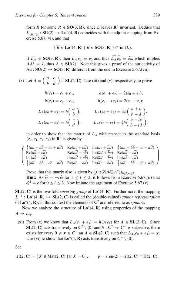
Exercises for Chapter 5: Tangent spaces 389
form R for some R ∈ SO(3,R), since L leaves R3 invariant. Deduce thatL|SU(2) : SU(2)→ Lo◦(4,R) coincides with the adjoint mapping from Ex-ercise 5.67.(vi), and that
{ R ∈ Lo◦(4,R) | R ∈ SO(3,R) } ⊂ im(L).
If L A ∈ SO(3,R), then L A e0 = e0 and thus L A e0 = e0, which impliesAA∗ = I , thus A ∈ SU(2). Note this gives a proof of the surjectivity ofAd : SU(2)→ SO(3,R) different from the one in Exercise 5.67.(vii).
(x) Let A =( a c
b d
)∈ SL(2,C). Use (iii) and (v), respectively, to prove
h(e1) = e0 + e3, h(e1 + e2) = 2(e0 + e1),
h(e2) = e0 − e3, h(e1 − ie2) = 2(e0 + e2);
L A(e0 + e3) = h( a
b
), L A(e0 + e1) = 1
2 h( a + c
b + d
),
L A(e0 − e3) = h( c
d
), L A(e0 + e2) = 1
2 h( a − ic
b − id
),
in order to show that the matrix of L A with respect to the standard basis(e0, e1, e2, e3) in R4 is given by12 (aa + bb + cc + dd) Re(ac + bd) Im(ac + bd) 1
2 (aa + bb − cc − dd)Re(ab + cd) Re(ad + cb) Im(ad + bc) Re(ab − cd)Im(ab + cd) Im(ad + cb) Re(ad − bc) Im(ab − cd)12 (aa − bb + cc − dd) Re(ac − bd) Im(ac − bd) 1
2 (aa − bb − cc + dd)
Prove that this matrix also is given by 1
2 ( tr(el Aem A∗))0≤l,m≤3.Hint: As el = −i el for 1 ≤ l ≤ 3, it follows from Exercise 5.67.(ii) thatel
2 = e for 0 ≤ l ≤ 3. Now imitate the argument of Exercise 5.67.(v).
SL(2,C) is the two-fold covering group of Lo◦(4,R). Furthermore, the mappingL−1 : Lo◦(4,R) → SL(2,C) is called the (double-valued) spinor representationof Lo◦(4,R); in this context the elements of C2 are referred to as spinors.
Now we analyze the structure of Lo◦(4,R) using properties of the mappingA �→ L A.
(xi) From (x) we know that L A(e0 + e3) = h(A e1) for A ∈ SL(2,C). SinceSL(2,C) acts transitively on C2 \ {0} and h : C2 → C+ is surjective, thereexists for every 0 = x ∈ C+ an A ∈ SL(2,C) such that L A(e0 + e3) = x.Use (vi) to show that Lo◦(4,R) acts transitively on C+ \ {0}.
Set
sl(2,C) = { X ∈ Mat(2,C) | tr X = 0 }, p = i su(2) = sl(2,C) ∩ H(2,C).
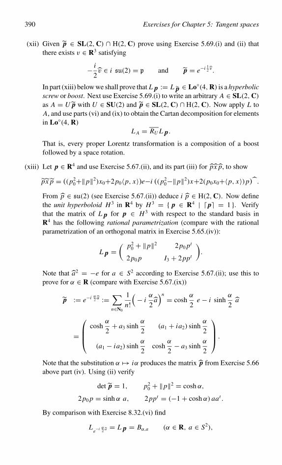
390 Exercises for Chapter 5: Tangent spaces
(xii) Given p ∈ SL(2,C) ∩ H(2,C) prove using Exercise 5.69.(i) and (ii) thatthere exists v ∈ R3 satisfying
− i
2v ∈ i su(2) = p and p = e−i 1
2 v .
In part (xiii) below we shall prove that L p := L p ∈ Lo◦(4,R) is a hyperbolicscrew or boost. Next use Exercise 5.69.(i) to write an arbitrary A ∈ SL(2,C)as A = U p with U ∈ SU(2) and p ∈ SL(2,C) ∩ H(2,C). Now apply L toA, and use parts (vi) and (ix) to obtain the Cartan decomposition for elementsin Lo◦(4,R)
L A = RU L p.
That is, every proper Lorentz transformation is a composition of a boostfollowed by a space rotation.
(xiii) Let p ∈ R4 and use Exercise 5.67.(ii), and its part (iii) for px p, to show
px p = ((p20+‖p‖2)x0+2p0〈p, x〉)e−i ((p2
0−‖p‖2)x+2(p0x0+〈p, x〉)p).From p ∈ su(2) (see Exercise 5.67.(ii)) deduce i p ∈ H(2,C). Now definethe unit hyperboloid H 3 in R4 by H 3 = { p ∈ R4 | ( p) = 1 }. Verifythat the matrix of L p for p ∈ H 3 with respect to the standard basis inR4 has the following rational parametrization (compare with the rationalparametrization of an orthogonal matrix in Exercise 5.65.(iv)):
L p =( p2
0 + ‖p‖2 2p0 pt
2p0 p I3 + 2ppt
).
Note that a2 = −e for a ∈ S2 according to Exercise 5.67.(ii); use this toprove for α ∈ R (compare with Exercise 5.67.(ix))
p := e−i α2 a :=
∑n∈N0
1
n!(− i
α
2a)n = cosh
α
2e − i sinh
α
2a
=
coshα
2+ a3 sinh
α
2(a1 + ia2) sinh
α
2
(a1 − ia2) sinhα
2cosh
α
2− a3 sinh
α
2
.
Note that the substitution α �→ iα produces the matrix p from Exercise 5.66above part (iv). Using (ii) verify
det p = 1, p20 + ‖p‖2 = cosh α,
2p0 p = sinh α a, 2ppt = (−1+ cosh α) aat .
By comparison with Exercise 8.32.(vi) find
Le−i α2 a = L p = Bα,a (α ∈ R, a ∈ S2),
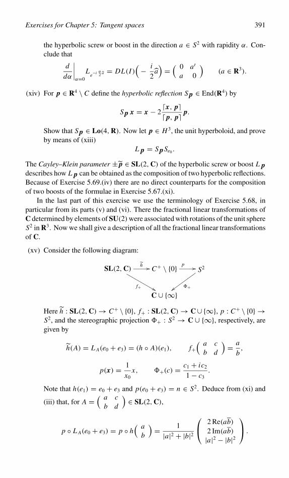
Exercises for Chapter 5: Tangent spaces 391
the hyperbolic screw or boost in the direction a ∈ S2 with rapidity α. Con-clude that
d
dα
∣∣∣∣α=0
Le−i α2 a = DL(I )
(− i
2a)=
( 0 at
a 0
)(a ∈ R3).
(xiv) For p ∈ R4 \ C define the hyperbolic reflection S p ∈ End(R4) by
S p x = x − 2(x, p)( p, p) p.
Show that S p ∈ Lo(4,R). Now let p ∈ H 3, the unit hyperboloid, and proveby means of (xiii)
L p = S pSe0 .
The Cayley–Klein parameter ± p ∈ SL(2,C) of the hyperbolic screw or boost L pdescribes how L p can be obtained as the composition of two hyperbolic reflections.Because of Exercise 5.69.(iv) there are no direct counterparts for the compositionof two boosts of the formulae in Exercise 5.67.(xi).
In the last part of this exercise we use the terminology of Exercise 5.68, inparticular from its parts (v) and (vi). There the fractional linear transformations ofC determined by elements of SU(2)were associated with rotations of the unit sphereS2 in R3. Now we shall give a description of all the fractional linear transformationsof C.
(xv) Consider the following diagram:
SL(2,C) h ��
f+ ������������ C+ \ {0} p �� S2
�+�����������
C ∪ {∞}Here h : SL(2,C)→ C+ \ {0}, f+ : SL(2,C)→ C∪ {∞}, p : C+ \ {0} →S2, and the stereographic projection �+ : S2 → C ∪ {∞}, respectively, aregiven by
h(A) = L A(e0 + e3) = (h ◦ A)(e1), f+( a c
b d
)= a
b,
p(x) = 1
x0x, �+(c) = c1 + ic2
1− c3.
Note that h(e1) = e0 + e3 and p(e0 + e3) = n ∈ S2. Deduce from (xi) and
(iii) that, for A =( a c
b d
)∈ SL(2,C),
p ◦ L A(e0 + e3) = p ◦ h( a
b
)= 1
|a|2 + |b|2
2 Re(ab)2 Im(ab)|a|2 − |b|2
.
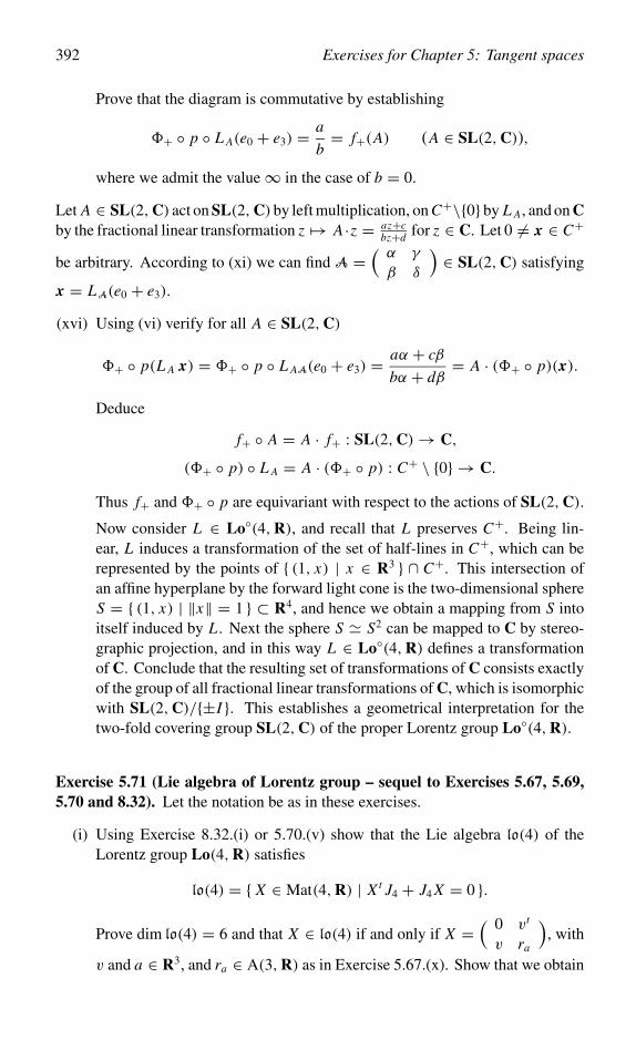
392 Exercises for Chapter 5: Tangent spaces
Prove that the diagram is commutative by establishing
�+ ◦ p ◦ L A(e0 + e3) = a
b= f+(A) (A ∈ SL(2,C)),
where we admit the value∞ in the case of b = 0.
Let A ∈ SL(2,C) act on SL(2,C)by left multiplication, on C+\{0}by L A, and on Cby the fractional linear transformation z �→ A ·z = az+c
bz+d for z ∈ C. Let 0 = x ∈ C+
be arbitrary. According to (xi) we can find A =(α γ
β δ
)∈ SL(2,C) satisfying
x = LA(e0 + e3).
(xvi) Using (vi) verify for all A ∈ SL(2,C)
�+ ◦ p(L A x) = �+ ◦ p ◦ L AA(e0 + e3) = aα + cβ
bα + dβ= A · (�+ ◦ p)(x).
Deduce
f+ ◦ A = A · f+ : SL(2,C)→ C,
(�+ ◦ p) ◦ L A = A · (�+ ◦ p) : C+ \ {0} → C.
Thus f+ and �+ ◦ p are equivariant with respect to the actions of SL(2,C).
Now consider L ∈ Lo◦(4,R), and recall that L preserves C+. Being lin-ear, L induces a transformation of the set of half-lines in C+, which can berepresented by the points of { (1, x) | x ∈ R3 } ∩ C+. This intersection ofan affine hyperplane by the forward light cone is the two-dimensional sphereS = { (1, x) | ‖x‖ = 1 } ⊂ R4, and hence we obtain a mapping from S intoitself induced by L . Next the sphere S � S2 can be mapped to C by stereo-graphic projection, and in this way L ∈ Lo◦(4,R) defines a transformationof C. Conclude that the resulting set of transformations of C consists exactlyof the group of all fractional linear transformations of C, which is isomorphicwith SL(2,C)/{±I }. This establishes a geometrical interpretation for thetwo-fold covering group SL(2,C) of the proper Lorentz group Lo◦(4,R).
Exercise 5.71 (Lie algebra of Lorentz group – sequel to Exercises 5.67, 5.69,5.70 and 8.32). Let the notation be as in these exercises.
(i) Using Exercise 8.32.(i) or 5.70.(v) show that the Lie algebra lo(4) of theLorentz group Lo(4,R) satisfies
lo(4) = { X ∈ Mat(4,R) | Xt J4 + J4 X = 0 }.
Prove dim lo(4) = 6 and that X ∈ lo(4) if and only if X =( 0 vt
v ra
), with
v and a ∈ R3, and ra ∈ A(3,R) as in Exercise 5.67.(x). Show that we obtain
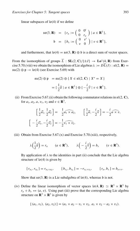
Exercises for Chapter 5: Tangent spaces 393
linear subspaces of lo(4) if we define
so(3,R) = { ra :=( 0 0t
0 ra
)| a ∈ R3 },
b = { bv :=( 0 vt
v 0
)| v ∈ R3 },
and furthermore, that lo(4) = so(3,R)⊕ b is a direct sum of vector spaces.
From the isomorphism of groups L : SL(2,C)/{±I } → Lo◦(4,R) from Exer-cise 5.70.(viii) we obtain the isomorphism of Lie algebras λ := DL(I ) : sl(2,R) =su(2)⊕ p → lo(4) (see Exercise 5.69) with
su(2)⊕ p = su(2)⊕ { X ∈ sl(2,C) | X∗ = X }
= { 1
2a | a ∈ R3 } ⊕ {− i
2v | v ∈ R3 }.
(ii) From Exercise 5.67.(ii) obtain the following commutator relations in sl(2,C),for a1, a2, a, v1, v2 and v ∈ R3,[ 1
2a1,
1
2a2
]= 1
2a1 × a2,
[ 1
2a,− i
2v]= − i
2a × v,
[− i
2v1,− i
2v2
]= −1
2v1 × v2.
(iii) Obtain from Exercise 5.67.(x) and Exercise 5.70.(xiii), respectively,
λ(1
2a)= ra (a ∈ R3), λ
(− i
2v)= bv (v ∈ R3).
By application of λ to the identities in part (ii) conclude that the Lie algebrastructure of lo(4) is given by
[ ra1, ra2 ] = ra1×a2, [ bv1, bv2 ] = −rv1×v2, [ ra, bv ] = ba×v.
Show that so(3,R) is a Lie subalgebra of lo(4), whereas b is not.
(iv) Define the linear isomorphism of vector spaces lo(4,R) � R3 × R3 byra + bv ↔ (a, v). Using part (iii) prove that the corresponding Lie algebrastructure on R3 × R3 is given by
[ (a1, v1), (a2, v2) ] = (a1 × a2 − v1 × v2, a1 × v2 − a2 × v1).
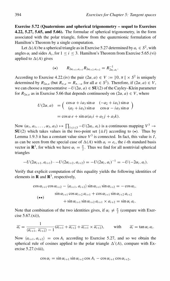
394 Exercises for Chapter 5: Tangent spaces
Exercise 5.72 (Quaternions and spherical trigonometry – sequel to Exercises4.22, 5.27, 5.65, and 5.66). The formulae of spherical trigonometry, in the formassociated with the polar triangle, follow from the quaternionic formulation ofHamilton’s Theorem by a single computation.
Let�(A) be a spherical triangle as in Exercise 5.27 determined by ai ∈ S2, withangles αi and sides Ai , for 1 ≤ i ≤ 3. Hamilton’s Theorem from Exercise 5.65.(vi)applied to �(A) gives
(�) R2αi+1,ai+1 R2αi+2,ai+2 = R−12αi ,ai
.
According to Exercise 4.22.(iv) the pair (2α, a) ∈ V := ] 0, π [ × S2 is uniquelydetermined by R2α,a (but Rπ,a = Rπ,−a for all a ∈ S2). Therefore, if (2α, a) ∈ V ,we can choose a representative−U (2α, a) ∈ SU(2) of the Cayley–Klein parameterfor R2α,a as in Exercise 5.66 that depends continuously on (2α, a) ∈ V , where
U (2α, a) =( cosα + ia3 sin α (−a2 + ia1) sin α
(a2 + ia1) sin α cosα − ia3 sin α
)= cosα e + sin α(a1i + a2 j + a3k).
Now (α1, a1, . . . , α3, a3) �→ ∏1≤i≤3−U (2αi , ai ) is a continuous mapping V 3 →
SU(2) which takes values in the two-point set {±I } according to (�). Thus byLemma 1.9.3 it has a constant value since V 3 is connected. In fact, this value is I ,as can be seen from the special case of �(A) with ai = ei , the i-th standard basisvector in R3, for which we have αi = π
2 . Thus we find for all nontrivial sphericaltriangles
−U (2αi+1, ai+1) · −U (2αi+2, ai+2) = −U (2αi , ai )−1 = −U (−2αi , ai ).
Verify that explicit computation of this equality yields the following identities ofelements in R and R3, respectively,
cosαi+1 cosαi+2 − 〈ai+1, ai+2〉 sin αi+1 sin αi+2 = − cosαi ,
(��)sin αi+1 cosαi+2 ai+1 + cosαi+1 sin αi+2 ai+2
+ sin αi+1 sin αi+2 ai+1 × ai+2 = sin αi ai .
Note that combination of the two identities gives, if αi = π2 (compare with Exer-
cise 5.67.(xi)),
ai = 1
〈ai+1, ai+2〉 − 1(ai+1 + ai+2 + ai+1 × ai+2), with ai = tan αi ai .
Now 〈ai+1, ai+2〉 = cos Ai according to Exercise 5.27, and so we obtain thespherical rule of cosines applied to the polar triangle �′(A), compare with Ex-ercise 5.27.(viii),
cosαi = sin αi+1 sin αi+2 cos Ai − cosαi+1 cosαi+2,
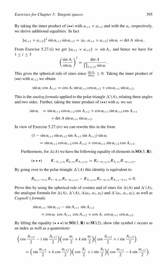
Exercises for Chapter 5: Tangent spaces 395
By taking the inner product of (��) with ai+1 × ai+2 and with the ai , respectively,we derive additional equalities. In fact
‖ai+1 × ai+2‖2 sin αi+1 sin αi+2 = 〈ai , ai+1 × ai+2〉 sin αi = det A sin αi .
From Exercise 5.27.(i) we get ‖ai+1 × ai+2‖ = sin Ai , and hence we have for1 ≤ i ≤ 3 (
sin Ai
sin αi
)2
= det A∏1≤i≤3 sin αi
.
This gives the spherical rule of sines since sin Aisin αi
≥ 0. Taking the inner product of(��) with ai+2 we obtain
sin αi cos Ai+1 = cos Ai sin αi+1 cosαi+2 + cosαi+1 sin αi+2.
This is the analog formula applied to the polar triangle �′(A), relating three anglesand two sides. Further, taking the inner product of (��) with ai we see
sin αi = sin αi+1 cosαi+2 cos Ai+2 + cosαi+1 sin αi+2 cos Ai+1
+ det A sin αi+1 sin αi+2.
In view of Exercise 5.27.(iv) we can rewrite this in the form
(1− sin αi+1 sin αi+2 sin Ai+1 sin Ai+2) sin αi
= sin αi+1 cosαi+2 cos Ai+2 + cosαi+1 sin αi+2 cos Ai+1.
Furthermore, for�(A)we have the following equality of elements in SO(3,R):
(� � �) R−Ai+1,e1 Rαi ,e3 RAi+2,e1 = Rπ−αi+2,e3 RAi ,e1 R−αi+1,e3 .
By going over to the polar triangle �′(A) this identity is equivalent to
Rαi+1−π,e1 Rπ−Ai ,e3 Rπ−αi+2,e1 − RAi+2,e3 Rπ−αi ,e1 RAi+1−π,e3 = 0.
Prove this by using the spherical rule of cosines and of sines for �(A) and �′(A),the analogue formula for �(A), �′(A), �(a1, a3, a2) and �′(a1, a3, a2), as well asCagnoli’s formula
sin αi+1 sin αi+2 − sin Ai+1 sin Ai+2
= cosαi cos Ai+1 cos Ai+2 + cos Ai cosαi+1 cosαi+2.
By lifting the equality (� � �) in SO(3,R) to SU(2), show (the symbol i occurs asan index as well as a quaternion)(
cosAi+1
2− i sin
Ai+1
2
)(cos
αi
2+ k sin
αi
2
)(cos
Ai+2
2+ i sin
Ai+2
2
)=
(sin
αi+2
2+ k cos
αi+2
2
)(cos
Ai
2+ i sin
Ai
2
)(cos
αi+1
2− k sin
αi+1
2
).
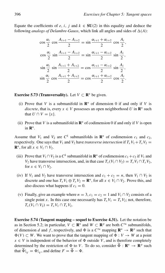
396 Exercises for Chapter 5: Tangent spaces
Equate the coefficients of e, i , j and k ∈ SU(2) in this equality and deduce thefollowing analogs of Delambre-Gauss, which link all angles and sides of �(A):
cosαi
2cos
Ai+1 − Ai+2
2= sin
αi+1 + αi+2
2cos
Ai
2,
cosαi
2sin
Ai+1 − Ai+2
2= sin
αi+1 − αi+2
2sin
Ai
2,
sinαi
2sin
Ai+1 + Ai+2
2= cos
αi+1 − αi+2
2sin
Ai
2,
sinαi
2cos
Ai+1 + Ai+2
2= cos
αi+1 + αi+2
2cos
Ai
2.
Exercise 5.73 (Transversality). Let V ⊂ Rn be given.
(i) Prove that V is a submanifold in Rn of dimension 0 if and only if V isdiscrete, that is, every x ∈ V possesses an open neighborhood U in Rn suchthat U ∩ V = {x}.
(ii) Prove that V is a submanifold in Rn of codimension 0 if and only if V is openin Rn .
Assume that V1 and V2 are Ck submanifolds in Rn of codimension c1 and c2,respectively. One says that V1 and V2 have transverse intersection if Tx V1+Tx V2 =Rn , for all x ∈ V1 ∩ V2.
(iii) Prove that V1∩V2 is a Ck submanifold in Rn of codimension c1+c2 if V1 andV2 have transverse intersection, and, in that case Tx(V1∩V2) = Tx V1∩Tx V2,for x ∈ V1 ∩ V2.
(iv) If V1 and V2 have transverse intersection and c1 + c2 = n, then V1 ∩ V2 isdiscrete and one has Tx V1 ⊕ Tx V2 = Rn , for all x ∈ V1 ∩ V2. Prove this, andalso discuss what happens if c1 = 0.
(v) Finally, give an example where n = 3, c1 = c2 = 1 and V1 ∩ V2 consists of asingle point x . In this case one necessarily has Tx V1 = Tx V2; not, therefore,Tx(V1 ∩ V2) = Tx V1 ∩ Tx V2.
Exercise 5.74 (Tangent mapping – sequel to Exercise 4.31). Let the notation beas in Section 5.2; in particular, V ⊂ Rn and W ⊂ Rp are both C∞ submanifolds,of dimension d and f , respectively, and � is a C∞ mapping Rn → Rp such that�(V ) ⊂ W . We want to prove that the tangent mapping of � : V → W at a pointx ∈ V is independent of the behavior of � outside V , and is therefore completelydetermined by the restriction of � to V . To do so, consider � : Rn → Rp suchthat �|V = �|V , and define F = �−�.
Exercises for Chapter 5: Tangent spaces 397
(i) Verify that the problem is a local one; in such a situation we may assumethat V = N (g, 0), with g : Rn → Rn−d a C∞ submersion. Now applyExercise 4.31 to the component functions Fi : Rn → R, for 1 ≤ i ≤ p, ofF . Conclude that, for every x0 ∈ V , there exist a neighborhood U of x0 inRn and C∞ mappings F (i) : U → Rp, with 1 ≤ i ≤ n − d, such that on U
F =∑
1≤i≤n−d
gi F (i).
(ii) Use Theorem 5.1.2 to prove, for every x ∈ V , the following equality ofmappings:
D�(x) = D�(x) ∈ Lin(Tx V, T�(x)W ).
Exercise 5.75 (“Intrinsic” description of tangent space). Let V be a Ck sub-manifold in Rn of dimension d and let x ∈ V . The definition of Tx V , the tangentspace to V at x , is independent of the description of V as a graph, parametrizedset, or zero-set. Once any such characterization of V has been chosen, however,Theorem 5.1.2 gives a corresponding description of Tx V . We now want to give an“intrinsic” description of Tx V . To find this, begin by assuming φ : Rd ⊃→ Rn andψ : Rd ⊃→ Rn are both Ck embeddings, with image V ∩ U , where U is an openneighborhood of x in Rn . Note that
φ(φ−1(x)) = ψ ◦ (ψ−1 ◦ φ)(φ−1(x)).
(i) Prove by immersivity of ψ in ψ−1(x) that, for two vectors v, w ∈ Rd , theequality of vectors in Rn
Dφ(φ−1(x))v = Dψ(ψ−1(x))w
holds if and only if
w = D(ψ−1 ◦ φ)(φ−1(x))v.
Next, define the coordinatizations κ := φ−1 : V ∩ U → Rd and λ := ψ−1 :V ∩U → Rd .
(ii) Prove
(�)∑
1≤ j≤d
v j D jφ(κ(x)) =∑
1≤k≤d
wk Dkψ(λ(x))
holds if and only if
(��) w = D(λ ◦ κ−1)(κ(x))v.
398 Exercises for Chapter 5: Tangent spaces
Note that v = (v1, . . . , vd) are the coordinates of the vector above in Tx V , withrespect to the basis vectors D jφ(κ(x)) (1 ≤ j ≤ d) for Tx V determined by κ .Condition (�) means that the pairs (v, κ) and (w, λ) represent the same vector inTx V ; and this is evidently the case if and only if (��) holds. Accordingly, we nowdefine the relation∼x on the set Rd × { coordinatizations of a neighborhood of x }by
(v, κ) ∼x (w, λ) ⇐⇒ relation (��) holds.
(iii) Prove that ∼x is an equivalence relation.
Denote the equivalence class of (v, κ) by [v, κ]x , and define Tx V as the collectionof these equivalence classes.
(iv) Verify that addition and scalar multiplication in Tx V
[v, κ]x + [v′, κ]x = [v + v′, κ]x , r [v, κ]x = [rv, κ]xare defined independent of the choice of the representatives; and that theseoperations make Tx V into a vector space.
(v) Prove that αx : Tx V → Tx V is a linear isomorphism, if
αx([v, κ]x) =∑
1≤ j≤d
v j D jφ(κ(x)).
Exercise 5.76 (Dual vector space, cotangent bundle, and differentials – neededfor Exercises 5.77 and 8.46). Let A be a vector space. We define the dual vectorspace A∗ as Lin(A,R).
(i) Prove that A∗∗ is linearly isomorphic with A.
(ii) Assume B is another vector space, and L ∈ Lin(A, B). Prove that the adjointlinear operator L∗ : B∗ → A∗ is a well-defined linear operator if
(L∗µ)(a) = µ(La) (µ ∈ B∗, a ∈ A).
Contrary to Section 2.1, in this case we do not use inner products to definethe adjoint of a linear operator, which explains the different notation.
(iii) Let dim A = d. Prove that dim A∗ = d and conclude that A is linearlyisomorphic with A∗ (in a noncanonical way).Hint: Choose a basis (a1, . . . , ad) for A, and define λ1, . . . , λd ∈ A∗ byλi (a j ) = δi j , for 1 ≤ i, j ≤ d, where δi j stands for the Kronecker delta.Check that (λ1, . . . , λd) forms a basis for A∗.
Exercises for Chapter 5: Tangent spaces 399
Assume that V is a C∞ submanifold in Rn of dimension d. As in Definition 4.7.3a function f : V → R is said to be a C∞ function on V if for every x ∈ V thereexist a neighborhood U of x in Rn , an open set D in Rd , and a C∞ embeddingφ : D → V ∩U such that f ◦ φ : D → R is a C∞ function. Let OV = O be thecollection of all C∞ functions on V .
(iv) Prove by Lemma 4.3.3.(iii) that this definition of O is independent of thechoice of the embeddings φ. Also prove that O is an algebra, for the oper-ations of pointwise addition and multiplication of functions, and pointwisemultiplication by scalars.
Let us assume for the moment that dim V = n; that is, V ⊂ Rn is an open set inRn . Then dim Tx V = n, and therefore Tx V in this case equals Rn , for all x ∈ V . Iff ∈ O, x ∈ V , this gives for the derivative D f (x) of f at x
D f (x) = (D1 f (x), . . . , Dn f (x)) ∈ Lin(Tx V,R).
We now write T ∗x V for the dual vector space of Tx V ; the vector space T ∗x V is alsoknown as the cotangent space of V at x . Consequently D f (x) ∈ T ∗x V . Furthermore,we write T ∗V =∐
x∈V T ∗x V for the disjoint union over all x ∈ V of the cotangentspaces of V at x . Here we ignore the fact that all these cotangent spaces are actuallycopies of the same space Rn , taking for every point x ∈ V a different copy of Rn .Then T ∗V is said to be the cotangent bundle of V . We can now assert that the totalderivative D f is a mapping from the manifold V to the cotangent bundle T ∗V ,
D f : V → T ∗V with D f : x �→ D f (x) ∈ T ∗x V .
We note that, in contrast to the present treatment, in Definition 2.2.2 of the derivativeone does not take the disjoint union of all cotangent spaces (� Rn), but one copyonly of Rn .
For the general case of dim V = d ≤ n we take inspiration from the resultabove. Let x = φ(y), with y ∈ D ⊂ Rd . We then have Tx V = im (Dφ(y)). Givenf ∈ O, x ∈ V , we define
dx f ∈ T ∗x V by dx f ◦ Dφ(y) = D( f ◦ φ)(y) : Rd → R.
The linear functional dx f ∈ T ∗x V is said to be the differential at x of the C∞function f on V .
(v) Check that dx f = D f (x), for all x ∈ V , if dim V = n.
Again we writeT ∗V =
∐x∈V
T ∗x V
for the disjoint union of the cotangent spaces. The reason for taking the disjointunion will now be apparent: the cotangent spaces might differ from each other, andwe do not wish to water this fact down by including into the union just one point
400 Exercises for Chapter 5: Tangent spaces
from among the points lying in each of these different cotangent spaces. Finally,define the differential d f of the C∞ function f on V as the mapping from themanifold V to the cotangent bundle T ∗V , given by
d f : V → T ∗V with d f : x �→ dx f ∈ T ∗x V .
A mapping V → T ∗V that assigns to x ∈ V an element of T ∗x V is said to be asection of the cotangent bundle T ∗V , or, alternatively, a differential form on V .Accordingly, d f is such a section of T ∗V , or a differential form on V . We finallyintroduce, for application in Exercise 5.77, the linear mapping
(�) dx : O → T ∗x V by dx : f �→ dx f (x ∈ V ).
(vi) Once more consider the case dim V = n. Verify that O contains the coordi-nate functions xi : x �→ xi , and that dx xi equals the 1× n matrix having a 1in the i-th column and 0 elsewhere, for x ∈ V and 1 ≤ i ≤ n. Conclude thatfor f ∈ O one has
d f =∑
1≤i≤n
Di f dxi .
Background. In Sections 8.6 – 8.8 we develop a more complete theory of differ-ential forms.
Exercise 5.77 (Algebraic description of tangent space – sequel to Exercise 5.76– needed for Exercise 5.78). The notation is as in that exercise. Let x ∈ V befixed. Then define Mx ⊂ O as the linear subspace of the f ∈ O with f (x) = 0;and define M2
x as the linear subspace in Mx generated by the products f g ∈ Mx ,where f , g ∈Mx .
(i) Check that Mx/M2x is a vector space.
(ii) Verify that dx from (�) in Exercise 5.76 induces dx ∈ Lin(Mx/M2x , T ∗x V )
(that is, M2x ⊂ ker dx ) such that the following diagram is commutative:
Mx T ∗x V
Mx/M2x
�
��
��� ��
���
dx
dx
(iii) Prove that dx ∈ Lin(Mx/M2x , T ∗x V ) is surjective.
Hint: For λ ∈ T ∗x V , consider the (locally defined) affine function f : V →R, given by
f ◦ φ(y′) = λ ◦ Dφ(y)(y′ − y) (y′ ∈ D).
Exercises for Chapter 5: Tangent spaces 401
Finally, we want to prove that dx ∈ Lin(Mx/M2x , T ∗x V ) is a linear isomorphism of
vector spaces, that is, one has (see Exercise 5.76.(i))
Tx V � (Mx/M2x)∗.
Therefore, what we have to prove is ker dx ⊂ M2x . Note that f ◦ φ(y) = 0 if
f ∈Mx .
(iv) Prove that for every f ∈ Mx there exist functions gi ∈ O, with 1 ≤ i ≤ d,such that for y′ ∈ D and g = (g1, . . . , gd),
f ◦ φ(y′) = 〈 g ◦ φ(y′), (y′ − y) 〉.
Hint: Compare with Exercise 4.31.(ii) and with the proof of the FourierInversion Theorem 6.11.6.
(v) Verify that for f ∈ ker dx one has D j ( f ◦ φ)(y) = 0, for 1 ≤ j ≤ d, andconclude by (iv) that this implies ker dx ⊂M2
x .
Background. The importance of this result is that it proves
(�) d = dimx V = dim Tx V = dim T ∗x V = dim(Mx/M2x);
and what is more, the algebra O contains complete information on the tangent spacesTx V . The following serves to illustrate this property.
Let V and V ′ be C∞ submanifolds in Rn and Rn′ of dimension d and d ′,respectively; let O and O′, respectively, be the associated algebras of C∞ functions.As in Definition 4.7.3 we say that a mapping of manifolds � : V → V ′ is a C∞mapping if for every x ∈ V there exist neighborhoods U of x in Rn and U ′ of�(x) inRn′ , open sets D ⊂ Rd and D′ ⊂ Rd ′ , and C∞ coordinatizations κ : V ∩U → Dand κ ′ : V ′ ∩ U ′ → D′, respectively, such that κ ′ ◦ � ◦ κ−1 : D ⊃→ Rd ′ is aC∞ mapping. Given such a mapping �, we have for every x ∈ V an inducedhomomorphism of rings
�∗x :M′�(x) →Mx given by �∗x( f ) = f ◦�.
(vi) Assume that for x ∈ V the mapping �∗x is a homomorphism of rings. Thenprove that � near x is a C∞ diffeomorphism of manifolds.Hint: By means of (�) one readily checks d = d ′. Without loss of generalitywe may assume that κ : V ∩ U → D ⊂ Rd is a C∞ coordinatization withκ(x) = 0, that is, κi ∈ Mx , for 1 ≤ i ≤ d. Consequently, then, there existfunctions λi ∈ M′
�(x) such that λi ◦ � = �∗x(λi ) = κi , for 1 ≤ i ≤ d.Hence λ ◦ � = κ in a neighborhood of x , if λ = (λ1, . . . , λd). Now, letκ ′ : V ′ ∩ U ′ → Rd be a C∞ coordinatization of a neighborhood of �(x).Then
(λ ◦ κ ′−1) ◦ (κ ′ ◦� ◦ κ−1)(κ(x)) = κ(x);
402 Exercises for Chapter 5: Tangent spaces
and so, by the chain rule,
D(λ ◦ κ ′−1)(κ ′(�(x))) ◦ D(κ ′ ◦� ◦ κ−1)(κ(x)) = I.
In particular, D(λ ◦ κ ′−1)(κ ′(�(x))) : Rd → Rd is surjective, and thereforeinvertible. According to the Local Inverse Function Theorem 3.2.4, λ ◦ κ ′−1
locally is a C∞ diffeomorphism; and therefore κ ′ ◦� ◦ κ−1 locally is a C∞diffeomorphism.
Exercise 5.78 (Lie derivative, vector field, derivation and tangent bundle –sequel to Exercise 5.77 – needed for Exercise 5.79). From Exercise 5.77 weknow that, for every x ∈ V , there exists a linear isomorphism
Tx V � (Mx/M2x)∗.
We will now give such an isomorphism in explicit form, in a way independent of thearguments from Exercise 5.77. Note that in Exercise 5.77 functions act on tangentvectors; we now show how tangent vectors act on functions.
We assume Tx V = im (Dφ(y)). For h = Dφ(y)v ∈ Tx V we define
Lx, h : O → R by Lx, h( f ) = dx f (h) = D( f ◦ φ)(y)v.Then Lx, h is called the Lie derivative at x in the direction of the tangent vectorh ∈ Tx V .
(i) Verify that Lx, h : O → R is a linear mapping satisfying
Lx, h( f g) = f (x)Lx, h(g)+ g(x)Lx, h( f ) ( f, g ∈ O).
We now abstract the properties of this Lie derivative in the following definition. Letδx : O → R be a linear mapping with the property
δx( f g) = f (x)δx(g)+ g(x)δx( f ) ( f, g ∈ O);then δx is said to be a derivation at the point x . In particular, therefore, Lx, h is aderivation at x , for all h ∈ Tx V .
(ii) Prove that δx(c) = 0, for every constant function c ∈ O, and conclude that,for every f ∈ O,
δx( f ) = δx( f − f (x)).
This result means that we may assume, without loss of generality, that a derivationat x acts on functions in Mx , instead of those in O.
(iii) Demonstrate
δx( f g) = 0 ( f, g ∈Mx); hence δx |M2x= 0.
Exercises for Chapter 5: Tangent spaces 403
We have, therefore, obtained
δx ∈ Lin(Mx/M2x , R); that is, δx ∈ (Mx/M
2x)∗.
Conversely, we may now conclude that, for a δx ∈ Lin(Mx/M2x , R), there is
exactly one derivation δx : O → R at x such that (with δx acting on representatives)
(�) δx |Mx= δx .
The existence of δx is found as follows. Given f ∈ O, one has f − f (x) ∈ Mx ,and hence we can define
δx( f ) := δx([ f − f (x)]).In particular, therefore, δx(c) = 0, for every constant function c ∈ O. Now, for f ,g ∈ O,
f g = ( f − f (x))(g − g(x))+ f (x)g + g(x) f − f (x)g(x);and because ( f − f (x))(g − g(x)) ∈ M2
x , it follows that
δx( f g) = f (x)δx(g)+ g(x)δx( f ).
In other words, δx is a derivation at x . Because a derivation at x always vanisheson the constant functions, we have that the derivation δx at x is uniquely defined by(�).
Finally, we prove that δx = Lx, X (x), for a unique element X (x) ∈ Tx V . Thisthen yields a linear isomorphism
X (x)↔ Lx, X (x) = δx ↔ δx so that Tx V � (Mx/M2x)∗.
To prove this, note that, as in Exercise 5.77.(iv), one has f − f (x) = 〈g, κ−κ(x)〉,with κ := φ−1.
(iv) Now verify that
δx( f ) =∑
1≤i≤n
gi (x) δx(κi − κi (x)) =∑
1≤i≤n
δx(κi − κi (x))Di ( f ◦ φ)(y)
=∑
1≤i≤n
δx(κi − κi (x) )Lx, ei ( f ) = Lx, X (x)( f ),
where X (x) =∑1≤i≤n δx(κi − κi (x))ei ∈ Tx V .
Next, we want to give a global formulation of the preceding results, that is, for allpoints x ∈ V at the same time. To do so, we define the tangent bundle T V of V by
T V =∐x∈V
Tx V,
404 Exercises for Chapter 5: Tangent spaces
where, as in Exercise 5.76, we take the disjoint union, but now of the tangentspaces. Further define a vector field on V as a section of the tangent bundle, thatis, as a mapping X : V → T V which assigns to x ∈ V an element X (x) ∈ Tx V .Additionally, introduce the Lie derivative L X in the direction of the vector field Xby
L X : O → O with L X ( f )(x) = Lx, X (x)( f ) ( f ∈ O, x ∈ V ).
And finally, define a derivation in O to be
δ ∈ End(O) satisfying δ( f g) = f δ(g)+ gδ( f ).
(v) Now proceed to demonstrate that, for every derivation δ in O, there exists aunique vector field X on V with
δ = L X , that is, δ( f )(x) = L X ( f )(x) ( f ∈ O, x ∈ V ).
We summarize the preceding as follows. Differential forms (sections of the cotan-gent bundle) and vector fields (sections of the tangent bundle) are dual to each other,and can be paired to a function on V . In particular, if d f is the differential of afunction f ∈ O and X is a vector field on V , then
d f (X) = L X ( f ) : V → R with d f (X)(x) = L X ( f )(x) = dx f (X (x)).
Exercise 5.79 (Pullback and pushforward under diffeomorphism – sequel toExercises 3.8 and 5.78). The notation is as in Exercise 5.78. Assume that V andU are both n-dimensional C∞ submanifolds (that is, open subsets) in Rn and that� : V → U is a C∞ diffeomorphism with �(y) = x . We introduce the linearoperator �∗ of pullback under the diffeomorphism � between the linear spaces ofC∞ functions on U and V by (compare with Definition 3.1.2)
�∗ : OU → OV with �∗( f ) = f ◦� ( f ∈ OU ).
Further, let W be open in Rn and let � : W → V be a C∞ diffeomorphism.
(i) Prove that (� ◦�)∗ = �∗ ◦�∗ : OU → OW .
We now define the induced linear operator �∗ of pushforward under the diffeo-morphism � between the linear spaces of derivations in OV and OU by means ofduality, that is
�∗ : Der(V )→ Der(U ), �∗(δ)( f ) = δ(�∗( f )) (δ ∈ Der(V ), f ∈ OU ).
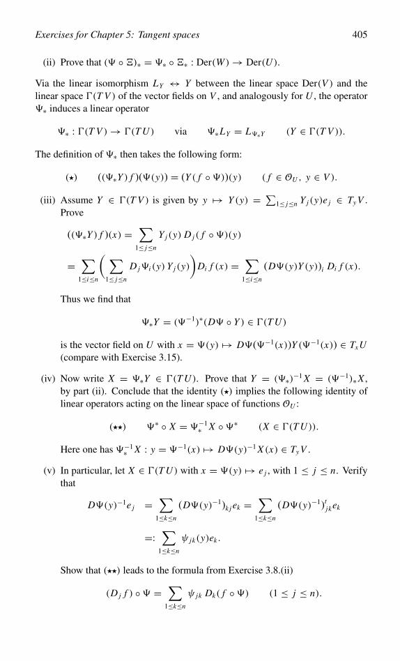
Exercises for Chapter 5: Tangent spaces 405
(ii) Prove that (� ◦�)∗ = �∗ ◦�∗ : Der(W )→ Der(U ).
Via the linear isomorphism LY ↔ Y between the linear space Der(V ) and thelinear space �(T V ) of the vector fields on V , and analogously for U , the operator�∗ induces a linear operator
�∗ : �(T V )→ �(T U ) via �∗LY = L�∗Y (Y ∈ �(T V )).
The definition of �∗ then takes the following form:
(�) ((�∗Y ) f )(�(y)) = (Y ( f ◦�))(y) ( f ∈ OU , y ∈ V ).
(iii) Assume Y ∈ �(T V ) is given by y �→ Y (y) = ∑1≤ j≤n Y j (y)e j ∈ Ty V .
Prove
((�∗Y ) f )(x) =∑
1≤ j≤n
Y j (y) D j ( f ◦�)(y)
=∑
1≤i≤n
( ∑1≤ j≤n
D j�i (y) Y j (y)
)Di f (x) =
∑1≤i≤n
(D�(y)Y (y))i Di f (x).
Thus we find that
�∗Y = (�−1)∗(D� ◦ Y ) ∈ �(T U )
is the vector field on U with x = �(y) �→ D�(�−1(x))Y (�−1(x)) ∈ TxU(compare with Exercise 3.15).
(iv) Now write X = �∗Y ∈ �(T U ). Prove that Y = (�∗)−1 X = (�−1)∗X ,by part (ii). Conclude that the identity (�) implies the following identity oflinear operators acting on the linear space of functions OU :
(��) �∗ ◦ X = �−1∗ X ◦�∗ (X ∈ �(T U )).
Here one has �−1∗ X : y = �−1(x) �→ D�(y)−1 X (x) ∈ Ty V .
(v) In particular, let X ∈ �(T U ) with x = �(y) �→ e j , with 1 ≤ j ≤ n. Verifythat
D�(y)−1e j =∑
1≤k≤n
(D�(y)−1)k j ek =∑
1≤k≤n
(D�(y)−1)tjkek
=:∑
1≤k≤n
ψ jk(y)ek .
Show that (��) leads to the formula from Exercise 3.8.(ii)
(D j f ) ◦� =∑
1≤k≤n
ψ jk Dk( f ◦�) (1 ≤ j ≤ n).
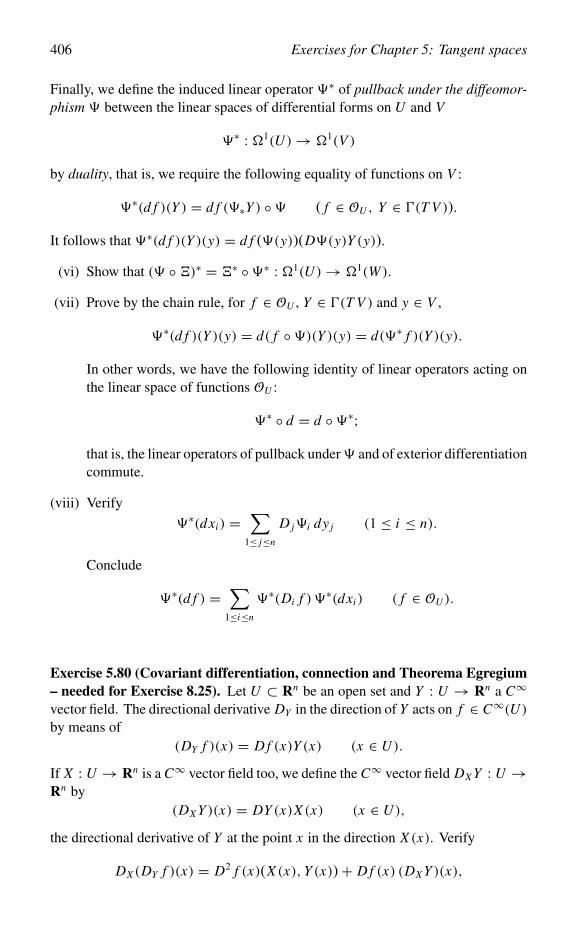
406 Exercises for Chapter 5: Tangent spaces
Finally, we define the induced linear operator �∗ of pullback under the diffeomor-phism � between the linear spaces of differential forms on U and V
�∗ : �1(U )→ �1(V )
by duality, that is, we require the following equality of functions on V :
�∗(d f )(Y ) = d f (�∗Y ) ◦� ( f ∈ OU , Y ∈ �(T V )).
It follows that �∗(d f )(Y )(y) = d f (�(y))(D�(y)Y (y)).
(vi) Show that (� ◦�)∗ = �∗ ◦�∗ : �1(U )→ �1(W ).
(vii) Prove by the chain rule, for f ∈ OU , Y ∈ �(T V ) and y ∈ V ,
�∗(d f )(Y )(y) = d( f ◦�)(Y )(y) = d(�∗ f )(Y )(y).
In other words, we have the following identity of linear operators acting onthe linear space of functions OU :
�∗ ◦ d = d ◦�∗;that is, the linear operators of pullback under� and of exterior differentiationcommute.
(viii) Verify
�∗(dxi ) =∑
1≤ j≤n
D j�i dy j (1 ≤ i ≤ n).
Conclude
�∗(d f ) =∑
1≤i≤n
�∗(Di f )�∗(dxi ) ( f ∈ OU ).
Exercise 5.80 (Covariant differentiation, connection and Theorema Egregium– needed for Exercise 8.25). Let U ⊂ Rn be an open set and Y : U → Rn a C∞vector field. The directional derivative DY in the direction of Y acts on f ∈ C∞(U )
by means of(DY f )(x) = D f (x)Y (x) (x ∈ U ).
If X : U → Rn is a C∞ vector field too, we define the C∞ vector field DX Y : U →Rn by
(DX Y )(x) = DY (x)X (x) (x ∈ U ),
the directional derivative of Y at the point x in the direction X (x). Verify
DX (DY f )(x) = D2 f (x)(X (x), Y (x))+ D f (x) (DX Y )(x),
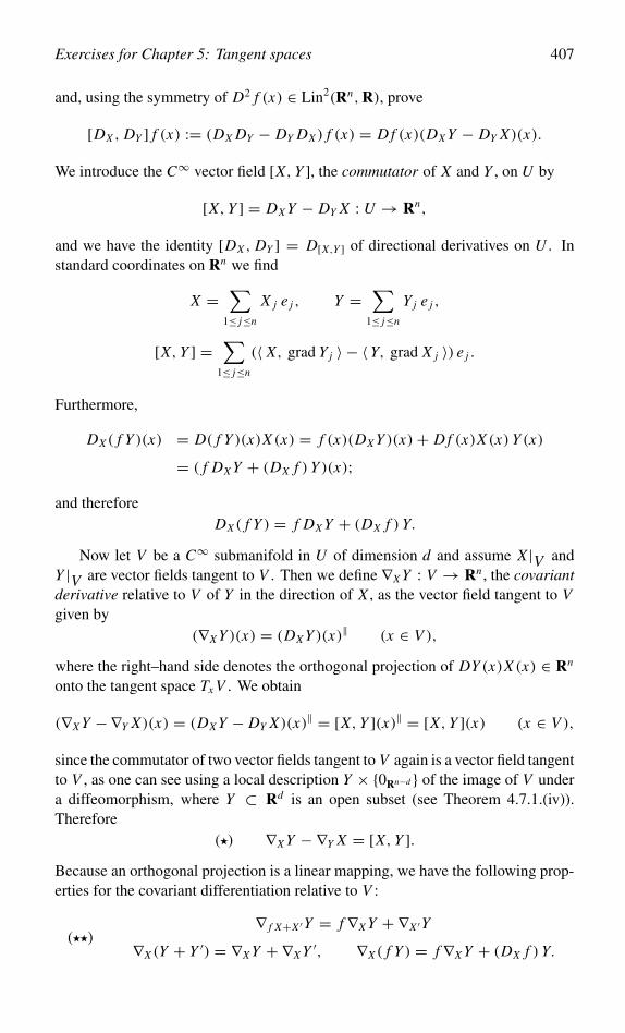
Exercises for Chapter 5: Tangent spaces 407
and, using the symmetry of D2 f (x) ∈ Lin2(Rn,R), prove
[DX , DY ] f (x) := (DX DY − DY DX ) f (x) = D f (x)(DX Y − DY X)(x).
We introduce the C∞ vector field [X, Y ], the commutator of X and Y , on U by
[X, Y ] = DX Y − DY X : U → Rn,
and we have the identity [DX , DY ] = D[X,Y ] of directional derivatives on U . Instandard coordinates on Rn we find
X =∑
1≤ j≤n
X j e j , Y =∑
1≤ j≤n
Y j e j ,
[X, Y ] =∑
1≤ j≤n
(〈 X, grad Y j 〉 − 〈 Y, grad X j 〉) e j .
Furthermore,
DX ( f Y )(x) = D( f Y )(x)X (x) = f (x)(DX Y )(x)+ D f (x)X (x) Y (x)
= ( f DX Y + (DX f ) Y )(x);and therefore
DX ( f Y ) = f DX Y + (DX f ) Y.
Now let V be a C∞ submanifold in U of dimension d and assume X |V andY |V are vector fields tangent to V . Then we define ∇X Y : V → Rn , the covariantderivative relative to V of Y in the direction of X , as the vector field tangent to Vgiven by
(∇X Y )(x) = (DX Y )(x)‖ (x ∈ V ),
where the right–hand side denotes the orthogonal projection of DY (x)X (x) ∈ Rn
onto the tangent space Tx V . We obtain
(∇X Y −∇Y X)(x) = (DX Y − DY X)(x)‖ = [X, Y ](x)‖ = [X, Y ](x) (x ∈ V ),
since the commutator of two vector fields tangent to V again is a vector field tangentto V , as one can see using a local description Y × {0Rn−d } of the image of V undera diffeomorphism, where Y ⊂ Rd is an open subset (see Theorem 4.7.1.(iv)).Therefore
(�) ∇X Y − ∇Y X = [X, Y ].Because an orthogonal projection is a linear mapping, we have the following prop-erties for the covariant differentiation relative to V :
(��)∇ f X+X ′Y = f∇X Y + ∇X ′Y
∇X (Y + Y ′) = ∇X Y +∇X Y ′, ∇X ( f Y ) = f∇X Y + (DX f ) Y.
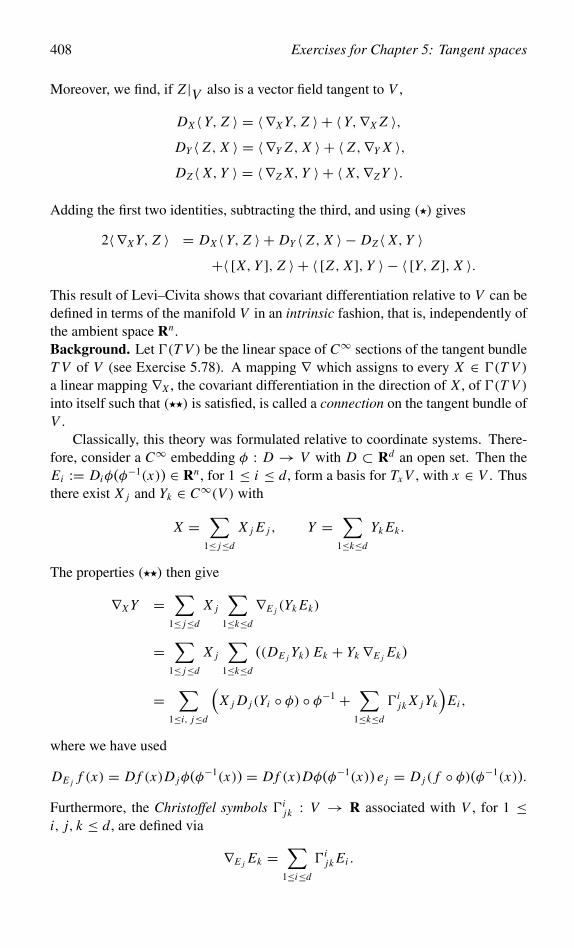
408 Exercises for Chapter 5: Tangent spaces
Moreover, we find, if Z |V also is a vector field tangent to V ,
DX 〈 Y, Z 〉 = 〈∇X Y, Z 〉 + 〈 Y,∇X Z 〉,DY 〈 Z , X 〉 = 〈∇Y Z , X 〉 + 〈 Z ,∇Y X 〉,DZ 〈 X, Y 〉 = 〈∇Z X, Y 〉 + 〈 X,∇Z Y 〉.
Adding the first two identities, subtracting the third, and using (�) gives
2〈 ∇X Y, Z 〉 = DX 〈 Y, Z 〉 + DY 〈 Z , X 〉 − DZ 〈 X, Y 〉+〈 [X, Y ], Z 〉 + 〈 [Z , X ], Y 〉 − 〈 [Y, Z ], X 〉.
This result of Levi–Civita shows that covariant differentiation relative to V can bedefined in terms of the manifold V in an intrinsic fashion, that is, independently ofthe ambient space Rn .Background. Let �(T V ) be the linear space of C∞ sections of the tangent bundleT V of V (see Exercise 5.78). A mapping ∇ which assigns to every X ∈ �(T V )a linear mapping ∇X , the covariant differentiation in the direction of X , of �(T V )into itself such that (��) is satisfied, is called a connection on the tangent bundle ofV .
Classically, this theory was formulated relative to coordinate systems. There-fore, consider a C∞ embedding φ : D → V with D ⊂ Rd an open set. Then theEi := Diφ(φ−1(x)) ∈ Rn , for 1 ≤ i ≤ d, form a basis for Tx V , with x ∈ V . Thusthere exist X j and Yk ∈ C∞(V ) with
X =∑
1≤ j≤d
X j E j , Y =∑
1≤k≤d
Yk Ek .
The properties (��) then give
∇X Y =∑
1≤ j≤d
X j
∑1≤k≤d
∇E j (Yk Ek)
=∑
1≤ j≤d
X j
∑1≤k≤d
((DE j Yk) Ek + Yk ∇E j Ek)
=∑
1≤i, j≤d
(X j D j (Yi ◦ φ) ◦ φ−1 +
∑1≤k≤d
�ijk X j Yk
)Ei ,
where we have used
DE j f (x) = D f (x)D jφ(φ−1(x)) = D f (x)Dφ(φ−1(x)) e j = D j ( f ◦ φ)(φ−1(x)).
Furthermore, the Christoffel symbols �ijk : V → R associated with V , for 1 ≤
i, j, k ≤ d, are defined via
∇E j Ek =∑
1≤i≤d
�ijk Ei .
Exercises for Chapter 5: Tangent spaces 409
Apparently, when differentiating Y covariantly relative to V in the direction of thetangent vector D jφ, one has to correct the Euclidean differentiations D j (Yi ◦φ) bycontributions
∑1≤k≤d �
ijkYk in terms of the Christoffel symbols associated with V .
From DEi E j = (Di D jφ)◦φ−1 we get [Ei , E j ] = 0, and so, for 1 ≤ i, j, k ≤ d,with gi j = 〈 Ei , E j 〉 and (gi j ) = (gi j )
−1,
�ijk =
1
2
∑1≤l≤d
gil(D j (glk ◦ φ)+ Dk(g jl ◦ φ)− Dl(g jk ◦ φ)) ◦ φ−1.
As an example consider the unit sphere S2, which occurs as an image underthe embedding φ(α, θ) = (cosα cos θ, sin α cos θ, sin θ). Then D1 D2φ(α, θ) =−(tan θ)D1φ(α, θ), from which
�112(φ(α, θ)) = − tan θ, �2
12(φ(α, θ)) = 0.
Or, equivalently
�112(x) = �1
21(x) = −x3√
1− x23
, �212(x) = �2
21(x) = 0 (x ∈ S2).
Finally, let d = n − 1 and assume that a continuous choice x �→ n(x) of anormal to V at x ∈ V has been made. Let 1 ≤ i, j ≤ n − 1 and let X be a vectorfield tangent to V , then
DEi DE j X = DEi (∇E j X + 〈 DE j X, n 〉n)= ∇Ei∇E j X + 〈 DE j X, n 〉DEi n + scalar multiple of n
= ∇Ei∇E j X − 〈 X, DE j n 〉DEi n + scalar multiple of n.
Now [DEi , DE j ] = D[Ei ,E j ] = 0. Interchanging the roles of i and j , subtracting,and taking the tangential component, we obtain
(� � �) (∇Ei∇E j − ∇E j∇Ei )X = 〈 X, DE j n 〉DEi n − 〈 X, DEi n 〉DE j n.
Since the left–hand side is defined intrinsically in terms of V , the same is true ofthe right–hand side in (� � �). The latter being trilinear, we obtain for every tripleof vector fields X , Y and Z tangent to V the following, intrinsically defined, vectorfield tangent to V :
〈 X, DY n 〉DZ n − 〈 X, DZ n 〉DY n.
Now apply the preceding to V ⊂ R3. Select Y and Z such that Y (x) and Z(x) forman orthonormal basis for Tx V , for every x ∈ V , and let X = Y . This gives for theGaussian curvature K of the surface V
K = det Dn = 〈 DY n, Y 〉〈 DZ n, Z 〉 − 〈 DY n, Z 〉〈 DZ n, Y 〉.Thus we have obtained Gauss’ Theorema Egregium (egregius = excellent) whichasserts that the Gaussian curvature of V is intrinsic.
410 Exercises for Chapter 5: Tangent spaces
Background. In the special case where dim V = n−1 the identity (� � �) suggeststhat the following mapping, where X , Y and Z are vector fields on V :
(X, Y, Z) �→ R(X, Y )Z = (∇X∇Y − ∇Y∇X − ∇[X,Y ])Zis trilinear over the functions on V , as is also true in general. Hence we can considerR as a mapping which assigns to tangent vectors X (x) and Y (x) ∈ Tx V the mappingZ(x) �→ R(X (x), Y (x))Z(x) belonging to Lin(Tx V, Tx V ); and the mapping actingon X (x) and Y (x) is bilinear and antisymmetric. Therefore R may be consideredas a differential 2-form on V (see the Remark following Proposition 8.1.12) withvalues in Lin (�(T V ), �(T V )); and this justifies calling R the curvature form ofthe connection ∇.
Notation
c complement 8◦ composition 17{·} closure 8∂ boundary 9∂V A boundary of A in V 11× cross product 147∇ nabla or del 59∇X covariant derivative in direction of X 407‖ · ‖ Euclidean norm on Rn 3‖ · ‖Eucl Euclidean norm on Lin(Rn,R p) 39〈 ·, · 〉 standard inner product 2[ ·, · ] Lie brackets 1691A characteristic function of A 34(α)k shifted factorial 180�i
jk Christoffel symbol 408� : U → V Ck diffeomorphism of open subsets U and V of Rn 88�∗ pushforward under diffeomorphism � 270� : V → U inverse mapping of � : U → V 88�∗ pullback under � 88At adjoint or transpose of matrix A 39A complementary matrix of A 41
AV
closure of A in V 11A(n,R) linear subspace of antisymmetric matrices in Mat(n,R) 159ad inner derivation 168Ad adjoint mapping 168Ad conjugation mapping 168arg argument function 88Aut(Rn) group of bijective linear mappings Rn → Rn 28, 38B(a; δ) open ball of center a and radius δ 6Ck k times continuously differentiable mapping 65codim codimension 112D j partial derivative, j-th 47D f derivative of mapping f 43D2 f (a) Hessian of f at a 71
411
412 Notation
d( ·, ·) Euclidean distance 5div divergence 166, 268dom domain space of mapping 108End(Rn) linear space of linear mappings Rn → Rn 38End+(Rn) linear subspace in End(Rn) of self-adjoint operators 41End−(Rn) linear subspace in End(Rn) of anti-adjoint operators 41f −1({·}) inverse image under f 12GL(n,R) general linear group, of invertible matrices 38
in Mat(n,R)grad gradient 59graph graph of mapping 107H(n,C) linear subspace of Hermitian matrices in Mat(n,C) 385I identity mapping 44im image under mapping 108inf infimum 21int interior 7L⊥ orthocomplement of linear subspace L 201lim limit 6, 12Lin(Rn,Rp) linear space of linear mappings Rn → Rp 38Link(Rn,R p) linear space of k-linear mappings Rn → Rp 63Lo◦(4,R) proper Lorentz group 386Mat(n,R) linear space of n × n matrices with coefficients in R 38Mat(p × n,R) linear space of p × n matrices with coefficients in R 38N (c) level set of c 15O = { Oi | i ∈ I } open covering of set 30O(Rn) orthogonal group, of orthogonal operators 73
in End(Rn)
O(n,R) orthogonal group, of orthogonal matrices 124in Mat(n,R)
Rn Euclidean space of dimension n 2Sn−1 unit sphere in Rn 124sl(n,C) Lie algebra of SL(n,C) 385SL(n,R) special linear group, of matrices in Mat(n,R) with 303
determinant 1SO(3,R) special orthogonal group, of orthogonal matrices 219
in Mat(3,R) with determinant 1SO(n,R) special orthogonal group, of orthogonal matrices 302
in Mat(n,R) with determinant 1su(2) Lie algebra of SU(2) 385SU(2) special unitary group, of unitary matrices 377
in Mat(2,C) with determinant 1sup supremum 21Tx V tangent space of submanifold V at point x 134T ∗V cotangent bundle of submanifold V 399T ∗x V cotangent space of submanifold V at point x 399tr trace 39V (a; δ) closed ball of center a and radius δ 8
Index
Abel’s partial summation formula 189Abel–Ruffini Theorem 102Abelian group 169acceleration 159action 238, 366—, group 162—, induced 163addition 2— formula for lemniscatic sine 288adjoint linear operator 39, 398— mapping 168, 380affine function 216Airy function 256Airy’s differential equation 256algebraic topology 307analog formula 395analogs of Delambre-Gauss 396angle 148, 219, 301— of spherical triangle 334angle-preserving 336angular momentum operator 230, 264,
272anti-adjoint operator 41anticommutative 169antisymmetric matrix 41approximation, best affine 44argument function 88associated Legendre function 177associativity 2astroid 324asymptotic expansion 197— expansion, Stirling’s 197automorphism 28autonomous vector field 163axis of rotation 219, 301
ball, closed 8—, open 6basis, orthonormal 3—, standard 3Bernoulli function 190
— number 186— polynomial 187Bernoulli’s summation formula 188,
194best affine approximation 44bifurcation set 289binomial coefficient, generalized 181— series 181binormal 159biregular 160bitangent 327boost 390boundary 9— in subset 11bounded sequence 21Brouwer’s Theorem 20bundle, tangent 322—, unit tangent 323
C1 mapping 51Cagnoli’s formula 395canonical 58Cantor’s Theorem 211cardioid 286, 299Cartan decomposition 247, 385Casimir operator 231, 265, 370catenary 295catenoid 295Cauchy sequence 22Cauchy’s Minimum Theorem 206Cauchy–Schwarz inequality 4— inequality, generalized 245caustic 351Cayley’s surface 309Cayley–Klein parameter 376, 380, 391chain rule 51change of coordinates, (regular) Ck 88characteristic function 34— polynomial 39, 239chart 111Christoffel symbol 408
413
414 Index
circle, osculating 361circles, Villarceau’s 327cissoid, Diocles’ 325Clifford algebra 383— multiplication 379closed ball 8— in subset 10— mapping 20— set 8closure 8— in subset 11cluster point 8— point in subset 10codimension of submanifold 112coefficient of matrix 38—, Fourier 190cofactor matrix 233commutativity 2commutator 169, 217, 231, 407— relation 231, 367compactness 25, 30—, sequential 25complement 8complementary matrix 41completeness 22, 204complex-differentiable 105component function 2— of vector 2composition of mappings 17computer graphics 385conchoid, Nicomedes’ 325conformal 336conjugate axis 330connected component 35connectedness 33connection 408conservation of energy 290continuity 13Continuity Theorem 77continuity, Hölder 213continuous mapping 13continuously differentiable 51contraction 23— factor 23Contraction Lemma 23convergence 6—, uniform 82convex 57coordinate function 19— of vector 2
coordinates, change of, (regular) Ck
88—, confocal 267—, cylindrical 260—, polar 88—, spherical 261coordinatization 111cosine rule 331cotangent bundle 399— space 399covariant derivative 407— differentiation 407covering group 383, 386, 389—, open 30Cramer’s rule 41critical point 60— point of diffeomorphism 92— point of function 128— point, nondegenerate 75— value 60cross product 147— product operator 363curvature form 363, 410— of curve 159—, Gaussian 157—, normal 162—, principal 157curve 110—, differentiable (space) 134—, space-filling 211cusp, ordinary 144cycloid 141, 293cylindrical coordinates 260
D’Alembert’s formula 277de l’Hôpital’s rule 311decomposition, Cartan 247, 385—, Iwasawa 356—, polar 247del 59Delambre-Gauss, analogs of 396DeMorgan’s laws 9dense in subset 203derivation 404— at point 402—, inner 169derivative 43—, directional 47—, partial 47derived mapping 43
Index 415
Descartes’ folium 142diameter 355diffeomorphism, Ck 88—, orthogonal 271differentiability 43differentiable mapping 43—, continuously 51—, partially 47differential 400— at point 399— equation, Airy’s 256— equation, for rotation 165— equation, Legendre’s 177— equation, Newton’s 290— equation, ordinary 55, 163, 177,
269— form 400— operator, linear partial 241— operator, partial 164Differentiation Theorem 78, 84dimension of submanifold 109Dini’s Theorem 31Diocles’ cissoid 325directional derivative 47Dirichlet’s test 189disconnectedness 33discrete 396discriminant 347, 348— locus 289distance, Euclidean 5distributivity 2divergence in arbitrary coordinates
268—, of vector field 166, 268dual basis for spherical triangle 334— vector space 398duality, definition by 404, 406duplication formula for (lemniscatic)
sine 180
eccentricity 330— vector 330Egregium, Theorema 409eigenvalue 72, 224eigenvector 72, 224elimination 125— theory 344elliptic curve 185— paraboloid 297embedding 111
endomorphism 38energy, kinetic 290—, potential 290—, total 290entry of matrix 38envelope 348epicycloid 342equality of mixed partial derivatives 62equation 97equivariant 384Euclidean distance 5— norm 3— norm of linear mapping 39— space 2Euler operator 231, 265Euler’s formula 300, 364— identity 228— Theorem 219Euler–MacLaurin summation formula
194evolute 350excess of spherical triangle 335exponential 55
fiber bundle 124— of mapping 124finite intersection property 32— part of integral 199fixed point 23flow of vector field 163focus 329folium, Descartes’ 142formula, analog 395—, Cagnoli’s 395—, D’Alembert’s 277—, Euler’s 300, 364—, Heron’s 330—, Leibniz–Hörmander’s 243—, Rodrigues’ 177—, Taylor’s 68, 250formulae, Frenet–Serret’s 160forward (light) cone 386Foucault’s pendulum 362four-square identity 377Fourier analysis 191— coefficient 190— series 190fractional linear transformation 384Frenet–Serret’s formulae 160Frobenius norm 39
416 Index
Frullani’s integral 81function of several real variables 12—, C∞, on subset 399—, affine 216—, Airy 256—, Bernoulli 190—, characteristic 34—, complex-differentiable 105—, coordinate 19—, holomorphic 105—, Lagrange 149—, monomial 19—, Morse 244—, piecewise affine 216—, polynomial 19—, positively homogeneous 203, 228—, rational 19—, real-analytic 70—, reciprocal 17—, scalar 12—, spherical 271—, spherical harmonic 272—, vector-valued 12—, zonal spherical 271functional dependence 312— equation 175, 313Fundamental Theorem of Algebra 291
Gauss mapping 156Gaussian curvature 157general linear group 38generalized binomial coefficient 181generator, infinitesimal 163geodesic 361geometric tangent space 135(geometric) tangent vector 322geometric–arithmetic inequality 351Global Inverse Function Theorem 93gradient 59— operator 59— vector field 59Gram’s matrix 39Gram–Schmidt orthonormalization
356graph 107, 203Grassmann’s identity 331, 364great circle 333greatest lower bound 21group action 162, 163, 238—, covering 383, 386, 389
—, general linear 38—, Lorentz 386—, orthogonal 73, 124, 219—, permutation 66—, proper Lorentz 386—, special linear 303—, special orthogonal 302—, special orthogonal, in R3 219—, special unitary 377—, spinor 383
Hadamard’s inequality 152, 356— Lemma 45Hamilton’s Theorem 375Hamilton–Cayley, Theorem of 240harmonic function 265Heine–Borel Theorem 30helicoid 296helix 107, 138, 296Hermitian matrix 385Heron’s formula 330Hessian 71— matrix 71highest weight of representation 371Hilbert’s Nullstellensatz 311Hilbert–Schmidt norm 39Hölder continuity 213Hölder’s inequality 353holomorphic 105holonomy 363homeomorphic 19homeomorphism 19homogeneous function 203, 228homographic transformation 384homomorphism of Lie algebras 170— of rings, induced 401Hopf fibration 307, 383— mapping 306hyperbolic reflection 391— screw 390hyperboloid of one sheet 298— of two sheets 297hypersurface 110, 145hypocycloid 342—, Steiner’s 343, 346
identity mapping 44—, Euler’s 228—, four-square 377—, Grassmann’s 331, 364
Index 417
—, Jacobi’s 332—, Lagrange’s 332—, parallelogram 201—, polarization 3—, symmetry 201image, inverse 12immersion 111— at point 111Immersion Theorem 114implicit definition of function 97— differentiation 103Implicit Function Theorem 100— Function Theorem over C 106incircle of Steiner’s hypocycloid 344indefinite 71index, of function at point 73—, of operator 73induced action 163— homomorphism of rings 401inequality, Cauchy–Schwarz’ 4—, Cauchy–Schwarz’, generalized
245—, geometric–arithmetic 351—, Hadamard’s 152, 356—, Hölder’s 353—, isoperimetric for triangle 352—, Kantorovich’s 352—, Minkowski’s 353—, reverse triangle 4—, triangle 4—, Young’s 353infimum 21infinitesimal generator 56, 163, 239,
303, 365, 366initial condition 55, 163, 277inner derivation 169integral formula for remainder in
Taylor’s formula 67, 68—, Frullani’s 81integrals, Laplace’s 254interior 7— point 7intermediate value property 33interval 33intrinsic property 408invariance of dimension 20— of Laplacian under orthogonal
transformations 230inverse image 12— mapping 55
irreducible representation 371isolated zero 45Isomorphism Theorem for groups 380isoperimetric inequality for triangle
352iteration method, Newton’s 235Iwasawa decomposition 356
Jacobi matrix 48Jacobi’s identity 169, 332— notation for partial derivative 48
k-linear mapping 63Kantorovich’s inequality 352
Lagrange function 149— multipliers 150Lagrange’s identity 332— Theorem 377Laplace operator 229, 263, 265, 270Laplace’s integrals 254Laplacian 229, 263, 265, 270— in cylindrical coordinates 263— in spherical coordinates 264latus rectum 330laws, DeMorgan’s 9least upper bound 21Lebesgue number of covering 210Legendre function, associated 177— polynomial 177Legendre’s equation 177Leibniz’ rule 240Leibniz–Hörmander’s formula 243Lemma, Hadamard’s 45—, Morse’s 131—, Rank 113lemniscate 323lemniscatic sine 180, 287— sine, addition formula for 288, 313length of vector 3level set 15Lie algebra 169, 231, 332— bracket 169— derivative 404— derivative at point 402— group, linear 166Lie’s product formula 171light cone 386limit of mapping 12— of sequence 6
418 Index
linear Lie group 166— mapping 38— operator, adjoint 39— partial differential operator 241— regression 228— space 2linearized problem 98Lipschitz constant 13— continuous 13Local Inverse Function Theorem 92— Inverse Function Theorem over C
105locally isometric 341Lorentz group 386— group, proper 386— transformation 386— transformation, proper 386lowering operator 371loxodrome 338
MacLaurin’s series 70manifold 108, 109— at point 109mapping 12—, C1 51—, k times continuously differentiable
65—, k-linear 63—, adjoint 380—, closed 20—, continuous 13—, derived 43—, differentiable 43—, identity 44—, inverse 55—, linear 38—, of manifolds 128—, open 20—, partial 12—, proper 26, 206—, tangent 225—, uniformly continuous 28—, Weingarten 157mass 290matrix 38—, antisymmetric 41—, cofactor 233—, Hermitian 385—, Hessian 71—, Jacobi 48
—, orthogonal 219—, symmetric 41—, transpose 39Mean Value Theorem 57Mercator projection 339method of least squares 248metric space 5minimax principle 246Minkowski’s inequality 353minor of matrix 41monomial function 19Morse function 244Morse’s Lemma 131Morsification 244moving frame 267multi-index 69Multinomial Theorem 241multipliers, Lagrange 150
nabla 59negative (semi)definite 71neighborhood 8— in subset 10—, open 8nephroid 343Newton’s Binomial Theorem 240— equation 290— iteration method 235Nicomedes’ conchoid 325nondegenerate critical point 75norm 27—, Euclidean 3—, Euclidean, of linear mapping 39—, Frobenius 39—, Hilbert–Schmidt 39—, operator 40normal 146— curvature 162— plane 159— section 162— space 139nullity, of function at point 73—, of operator 73Nullstellensatz, Hilbert’s 311
one-parameter family of lines 299— group of diffeomorphisms 162— group of invertible linear mappings
56— group of rotations 303
Index 419
open ball 6— covering 30— in subset 10— mapping 20— neighborhood 8— neighborhood in subset 10— set 7operator norm 40—, anti-adjoint 41—, self-adjoint 41orbit 163orbital angular momentum quantum
number 272ordinary cusp 144— differential equation 55, 163, 177,
269orthocomplement 201orthogonal group 73, 124, 219— matrix 219— projection 201— transformation 218— vectors 2orthonormal basis 3orthonormalization, Gram–Schmidt
356osculating circle 361— plane 159
℘ function, Weierstrass’ 185paraboloid, elliptic 297parallel translation 363parallelogram identity 201parameter 97—, Cayley–Klein 376, 380, 391parametrization 111—, of orthogonal matrix 364, 375parametrized set 108partial derivative 47— derivative, second-order 61— differential operator 164— differential operator, linear 241— mapping 12— summation formula of Abel 189partial-fraction decomposition 183partially differentiable 47particle without spin 272pendulum, Foucault’s 362periapse 330period 185— lattice 184, 185
periodic 190permutation group 66perpendicular 2physics, quantum 230, 272, 366piecewise affine function 216planar curve 160plane, normal 159—, osculating 159—, rectifying 159Pochhammer symbol 180point of function, critical 128— of function, singular 128—, cluster 8—, critical 60—, interior 7—, saddle 74—, stationary 60Poisson brackets 242polar coordinates 88— decomposition 247— part 247— triangle 334polarization identity 3polygon 274polyhedron 274polynomial function 19—, Bernoulli 187—, characteristic 39, 239—, Legendre 177—, Taylor 68polytope 274positive (semi)definite 71positively homogeneous function 203,
228principal curvature 157— normal 159principle, minimax 246product of mappings 17—, cross 147—, Wallis’ 184projection, Mercator 339—, stereographic 336proper Lorentz group 386— Lorentz transformation 386— mapping 26, 206property, global 29—, local 29pseudosphere 358pullback 406— under diffeomorphism 88, 268, 404
420 Index
pushforward under diffeomorphism270, 404
Pythagorean property 3
quadric, nondegenerate 297quantum number, magnetic 272— physics 230, 272, 366quaternion 382
radial part 247raising operator 371Rank Lemma 113rank of operator 113Rank Theorem 314rational function 19— parametrization 390Rayleigh quotient 72real-analytic function 70reciprocal function 17rectangle 30rectifying plane 159reflection 374regression line 228regularity of mapping Rd ⊃→ Rn 116— of mapping Rn ⊃→ Rn−d 124— of mapping Rn ⊃→ Rn 92regularization 199relative topology 10remainder 67representation, highest weight of 371—, irreducible 371—, spinor 383resultant 346reverse triangle inequality 4revolution, surface of 294Riemann’s zeta function 191, 197Rodrigues’ formula 177— Theorem 382Rolle’s Theorem 228rotation group 303—, in R3 219, 300—, in Rn 303—, infinitesimal 303rule, chain 51—, cosine 331—, Cramer’s 41—, de l’Hôpital’s 311—, Leibniz’ 240—, sine 331—, spherical, of cosines 334
—, spherical, of sines 334
saddle point 74scalar function 12— multiple of mapping 17— multiplication 2Schur complement 304second derivative test 74second-order derivative 63— partial derivative 61section 400, 404—, normal 162segment of great circle 333self-adjoint operator 41semicubic parabola 144, 309semimajor axis 330semiminor axis 330sequence, bounded 21sequential compactness 25series, binomial 181—, MacLaurin’s 70—, Taylor’s 70set, closed 8—, open 7shifted factorial 180side of spherical triangle 334signature, of function at point 73—, of operator 73simple zero 101sine rule 331singular point of diffeomorphism 92— point of function 128singularity of mapping Rn ⊃→ Rn 92slerp 385space, linear 2—, metric 5—, vector 2space-filling curve 211, 214special linear group 303— orthogonal group 302— orthogonal group in R3 219— unitary group 377Spectral Theorem 72, 245, 355sphere 10spherical coordinates 261— function 271— harmonic function 272— rule of cosines 334— rule of sines 334— triangle 333
Index 421
spinor 389— group 383— representation 383, 389spiral 107, 138, 296—, logarithmic 350standard basis 3— embedding 114— inner product 2— projection 121stationary point 60Steiner’s hypocycloid 343, 346— Roman surface 307stereographic projection 306, 336Stirling’s asymptotic expansion 197stratification 304stratum 304subcovering 30—, finite 30subimmersion 315submanifold 109— at point 109—, affine algebraic 128—, algebraic 128submersion 112— at point 112Submersion Theorem 121sum of mappings 17summation formula of Bernoulli 188,
194— formula of Euler–MacLaurin 194supremum 21surface 110— of revolution 294—, Cayley’s 309—, Steiner’s Roman 307Sylvester’s law of inertia 73— Theorem 376symbol, total 241symmetric matrix 41symmetry identity 201
tangent bundle 322, 403— mapping 137, 225— space 134— space, algebraic description 400— space, geometric 135— space, “intrinsic” description 397— vector 134— vector field 163— vector, geometric 322
Taylor polynomial 68Taylor’s formula 68, 250— series 70test, Dirichlet’s 189tetrahedron 274Theorem, Abel–Ruffini’s 102—, Brouwer’s 20—, Cantor’s 211—, Cauchy’s Minimum 206—, Continuity 77—, Differentiation 78, 84—, Dini’s 31—, Euler’s 219—, Fundamental, of Algebra 291—, Global Inverse Function 93—, Hamilton’s 375—, Hamilton–Cayley’s 240—, Heine–Borel’s 30—, Immersion 114—, Implicit Function 100—, Implicit Function, over C 106—, Isomorphism, for groups 380—, Lagrange’s 377—, Local Inverse Function 92—, Local Inverse Function, over C 105—, Mean Value 57—, Multinomial 241—, Newton’s Binomial 240—, Rank 314—, Rodrigues’ 382—, Rolle’s 228—, Spectral 72, 245, 355—, Submersion 121—, Sylvester’s 376—, Weierstrass’ Approximation 216Theorema Egregium 409thermodynamics 290tope, standard (n + 1)- 274topology 10—, algebraic 307—, relative 10toroid 349torsion 159total derivative 43— symbol 241totally bounded 209trace 39tractrix 357transformation, orthogonal 218transition mapping 118
422 Index
transpose matrix 39transversal 172transverse axis 330— intersection 396triangle inequality 4— inequality, reverse 4trisection 326tubular neighborhood 319
umbrella, Whitney’s 309uniform continuity 28— convergence 82uniformly continuous mapping 28unit hyperboloid 390— sphere 124— tangent bundle 323unknown 97
value, critical 60vector field 268, 404
— field, gradient 59— space 2vector-valued function 12Villarceau’s circles 327
Wallis’ product 184wave equation 276Weierstrass’ ℘ function 185— Approximation Theorem 216Weingarten mapping 157Whitney’s umbrella 309Wronskian 233
Young’s inequality 353
Zeeman effect 272zero, simple 101zero-set 108zeta function, Riemann’s 191, 197zonal spherical function 271


![10-1 Lesson 10 Objectives Chapter 4 [1,2,3,6]: Multidimensional discrete ordinates Chapter 4 [1,2,3,6]: Multidimensional discrete ordinates Multidimensional](https://img.pdfslide.us/doc/110x75/5697bff81a28abf838cbf777/10-1-lesson-10-objectives-chapter-4-1236-multidimensional-discrete-ordinates.jpg)