Multidimensional Data-Sets for Sound Applications

Ioannis Tsirikoglou

Master’s Thesis Institute of Sonology

Den Haag May 2012

2

Acknowledgments I would like to thank: My mentor, Paul Berg. Without his help, comments and support this thesis would not

have been realized. All my teachers in the Institute of Sonology: Kees Tazelaar, Richard Barrett, Johan van

Kreij, Peter Pabon, Raviv Ganchrow and Joel Ryan. They all provided me with great knowledge and inspiration.

My good friends Angel Faraldo and Aurimas Bavarskis for reading and commenting on my thesis.

All my colleagues in the Institute of Sonology and my friends (in the Netherlands as well as in Greece).

Finally I would especially like to thank my parents for their support and understanding. © Ioannis Tsirikoglou 2012

3

Contents 1. Introduction ………………………………………………………...……..…5

2. Generating Form …………………………………………………………....8

2.1 In Between Music and Architecture ……………………………………..…..8

2.2 Algorithms, Nature and Morphogenesis ………………......…………..…11

2.3 Formalizing Macro and Micro Structures ………………….................14

2.4 Graphic Representations, Complexity and Intuition .........................18

3. Multidimensional Data Sets ……………………………………………. 23

3.1 Wave Terrain Sythesis ………………………………………………………..24

3.2 Virtual Navigation of Parameter Spaces ……………………………..…..29

3.3 From Instrument Design to Compositional Form. Nomos Alpha. …… 32

3.4 Generative Scores and Worlds ……………………………………………. 37

4. Mapping ……………………………………………………………………..40

4.1 Composing Mappings………………………………………………………....40

4.1.1 General……………………………………………………………………………40

4.1.2 Mapping and Interactivity …………………………………………….……. 42

4.1.3 Mapping and Composition. Composed Instruments ……………….….. 44

4.2 Mapping Strategies ……………………………………………………..….. 46

4.2.1 Mapping with Matrices ……………………………………………… ……… 47

4.2.2 Linear Mapping ............................................................................ 48

4.2.3 Non-Linear Mapping ……………………………………………… ………….49

5. Sculpting Space ……………………………………………………………52

5.1 Spatial Composition…………………………………………………..………..52

4

5.2 Spatial Sound Synthesis………………………………………………………..56

6. ModTools…………………………………………………………………….60

6.1 Concept ………………………………………………………………………….60

6.2 Implementation …………………………………………………………………61

6.2.1 ViMod ……………………………………………………………………………62

6.2.2.KineMod …………………………………………………………………… …..67

6.2.3.MapMods …………………………………………………………………...….69

6.2.4.SpaceMod …….…………………………………………………………….... 71

6.3 Applications …………………………………………………………………....72

6.3.1 SpaceTextures ………………………………………………………………….72

6.3.2 SpaceScrubber …………………………………………………………..……73

Conclusions and further development ……………………………….…. 75

References………………………………………………………………..…....77

Appendix: Contents of accompanying DVD…………………………………..82

5

1. Introduction

The use of algorithms in the arts can be as old as the use of mathematical and logical

abstractions in order to observe and understand the world. Especially relationships between

music and mathematics can already be found in ancient Greece. Some of the concepts of

Pythagoras are still present in music theory. Pythagoras introduced the use of mathematics in

his philosophy, combining the irrational, religious thinking of ancient Greek thought with

mathematical rationalism. Pythagoras was searching for harmony and global proportions in

numbers since “all things are numbers, furnished with numbers or similar to numbers”

(Xenakis 1992, p 202). The Pythagorean tuning, where frequency relationships of all the

intervals are based on a 3:2 ratio, was used for many years and defines the base for the twelve

tone equal temperament. “Musica Universalis” or “Harmony of the spheres" is another

harmonic, mathematical and even religious concept where the proportions in the movements

of celestial bodies, Sun Moon and planets, form a kind of music. This music is not audible,

though this hum or resonance of the planets’ orbital revolutions can affect the quality of life

on earth. Similar concepts, like the Golden Ratio, which combine a rational or mathematical

way of creating proportions with a metaphysical given meaning, have been commonly used

through the centuries in music, architecture and visual arts.

With the development of sciences and especially with the help of computers our

knowledge on the mechanisms of nature goes deeper. We are able to explain very complex

natural phenomena, handle huge amount of information and perform calculations that would

6

be impossible to do by hand. A, similar to Pythagoreans, intellectual approach for the arts (by

using algorithms as basic structures to create proportions and harmonies) is more than present

in our modern culture. Mathematical models constitute inspiration for creating new forms in

music, architecture and visual arts. New geometries, curves, hyper surfaces, dynamical

systems, chaotic functions, fractals, evolutionary systems and genetic algorithms, cellular

automata and formal grammars (like L-Systems) are just some of the various mathematical

models that express the beautiful complexity of nature and have been used in numerous

artistic applications. The human creativity that is hiding behind selecting, combining and

manipulating mathematical models and mapping them to material in order to form new

structures, will always have a metaphysical character, maybe as art itself. Is interesting that

the same algorithms, as being fascinating for their morphologies and their temporal

evolution, have been applied on different sections of art like music and architecture.

Especially in modern architecture the meaning of time is being redefined, fact that brings

architectural form closer to the dynamic character of musical form.

“For a long time architecture was thought of as a solid reality and entity: buildings,

objects, matter, place, and a set of geometric relationships. But recently, architects

have begun to understand their products as liquid, animating their bodies,

hypersurfacing their walls, crossbreeding different locations, experimenting with new

geometries. And this is only the beginning.” (Bouman, 2005, p.22)

Generative architectural design shares common ground with computer music, the

same generative tools are used for both arts, like the Max/Msp/Jitter environment, and

common mathematical models define many of their structural elements. New media research

is giving us impressive three dimensional environments, where visuals, as dynamic

architectural forms, are combined with surround sound in order to create immersive, even

navigable, illusions of new, imaginary, though “naturally” complex, worlds.

Considering the differences in our visual and aural perception, as we are experiencing

architectural and musical structures, several questions are rising about the use of algorithms

for the creation and evolution of form in the arts. How mathematical models are participating

in the emergence and temporal development of form? How nature is involved? What is the

meaning of time in such processes? How new forms can occur? How architectural form is

connected with musical form? How graphic representations (as architectural or visual forms)

7

can help us to formalize sound and how can we use visual manipulations to intuitively act on

sound and handle complexity?

In the second chapter of the thesis an attempt to answer those questions has been

made. Emphasis is given in the works of Iannis Xenakis and other composers that are dealing

with ontological explorations concerning form in algorithmic composition and generative

computer music, as well as Sanford Kwinter’s philosophical ideas on morphogenesis in the

arts. Under this theoretical framework, techniques and compositional ideas that deal with

multidimensional representations of mathematical models and navigation of three

dimensional, or architectural, spaces in order to intuitively control sound material are

presented in the third chapter. The role and the importance of mapping, as a transfer function

to connect basic algorithmic structures with musical parameters, is discussed in the fourth

chapter, as well as some contemporary approaches on mapping using matrices. In the fifth

chapter the use of space for sound applications is investigated and several approaches on

spatial composition and spatial sound synthesis are presented.

Unifying all the above ideas, the result of this research is presented further. A general

set of tools that allow us to design dynamic, immersive sonic sctructures. Those tools have

been designed under a modular approach in the Max/Msp/Jitter programming environment so

they can be combined with any object or existing patch. The basic module is a host for

creating three-dimensional visual representations of mathematical models. Information is

extracted, as we trace those shapes in all possible time scales, and it can be mapped to any

musical parameter using the special mapping modules, as well as can define spatial position

of sounds in 2d or 3d spatial rendering systems. Geometrical transformations and

interpolations allow us to transform those trajectories and accordingly the mapped

parameters. The idea is to extract the special morphologies of different algorithms and their

unique development in time, create patterns in many layers and different time scales, act on

many parameters at the same time and define spatial movements. In this way we can “sculpt”

sounds in space, we can create alive, evolving sonic entities with natural characteristics.

8

2. Generating Form

2.1 In Between Music and Architecture

Seeking for relationships between the use of mathematical models, their graphic

representations and the production of new musical forms in surround sound environments we

unavoidably turn into Iannis Xenakis ideas as his full body of musical and architectural work

deals with such relationships. The intersection between music and architecture in Xenakis

work can help us reveal the concepts that are hiding behind, what inspires him, how spatial

formations - transformations and arrangements of those concepts are participating in

producing new musical forms in (architectural) space and what is the role of mathematics

when dealing with the arts.

Sterken (2007) is pointing two speculations about the intersection of music and

architecture. The first is the intellectual, as introduced by ancient Greek thought and is linked

with the problems of form and structure. In the Renaissance, this combination of rationalism

and metaphysics into searching for global underlying structures, like the theory of ‘harmonic

proportions’, knew his peak as many architects and composers tried to shape architectural or

musical form under the same numerical principles. The second speculation is the

phenomenological, coming from the 18th century aesthetic relativism, where the expressive

quality of art arise from its aesthetic effect and its immersive power. (Sterken, 2007, p.21)

9

Xenakis includes in his work both the intellectual, by trying to establish “universal”

underlying structures coming from new scientific - mathematical theories, and the

phenomenological by combining different structures to form immersive art that surrounds the

listener.

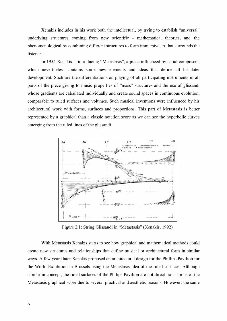
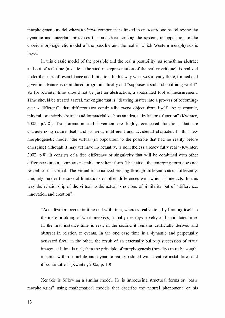
In 1954 Xenakis is introducing “Metastasis”, a piece influenced by serial composers,

which nevertheless contains some new elements and ideas that define all his later

development. Such are the differentiations on playing of all participating instruments in all

parts of the piece giving to music properties of “mass” structures and the use of glissandi

whose gradients are calculated individually and create sound spaces in continuous evolution,

comparable to ruled surfaces and volumes. Such musical inventions were influenced by his

architectural work with forms, surfaces and proportions. This part of Metastasis is better

represented by a graphical than a classic notation score as we can see the hyperbolic curves

emerging from the ruled lines of the glissandi.

Figure 2.1: String Glissandi in “Metastasis” (Xenakis, 1992)

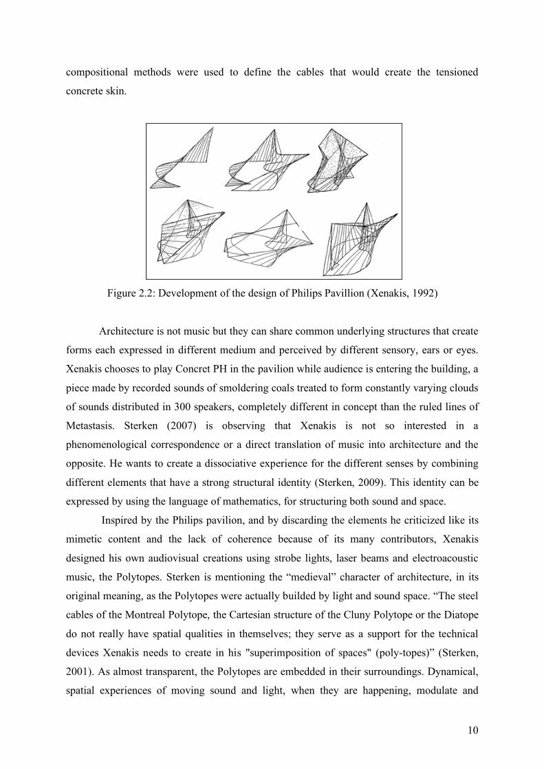
With Metastasis Xenakis starts to see how graphical and mathematical methods could

create new structures and relationships that define musical or architectural form in similar

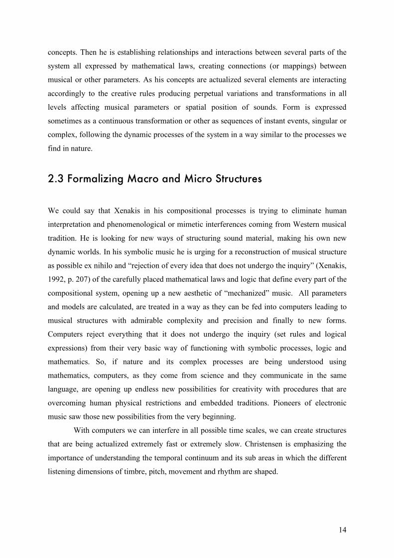
ways. A few years later Xenakis proposed an architectural design for the Phillips Pavilion for

the World Exhibition in Brussels using the Metastasis idea of the ruled surfaces. Although

similar in concept, the ruled surfaces of the Philips Pavilion are not direct translations of the

Metastasis graphical score due to several practical and aesthetic reasons. However, the same

10

compositional methods were used to define the cables that would create the tensioned

concrete skin.

Figure 2.2: Development of the design of Philips Pavillion (Xenakis, 1992)

Architecture is not music but they can share common underlying structures that create

forms each expressed in different medium and perceived by different sensory, ears or eyes.

Xenakis chooses to play Concret PH in the pavilion while audience is entering the building, a

piece made by recorded sounds of smoldering coals treated to form constantly varying clouds

of sounds distributed in 300 speakers, completely different in concept than the ruled lines of

Metastasis. Sterken (2007) is observing that Xenakis is not so interested in a

phenomenological correspondence or a direct translation of music into architecture and the

opposite. He wants to create a dissociative experience for the different senses by combining

different elements that have a strong structural identity (Sterken, 2009). This identity can be

expressed by using the language of mathematics, for structuring both sound and space.

Inspired by the Philips pavilion, and by discarding the elements he criticized like its

mimetic content and the lack of coherence because of its many contributors, Xenakis

designed his own audiovisual creations using strobe lights, laser beams and electroacoustic

music, the Polytopes. Sterken is mentioning the “medieval” character of architecture, in its

original meaning, as the Polytopes were actually builded by light and sound space. “The steel

cables of the Montreal Polytope, the Cartesian structure of the Cluny Polytope or the Diatope

do not really have spatial qualities in themselves; they serve as a support for the technical

devices Xenakis needs to create in his "superimposition of spaces" (poly-topes)” (Sterken,

2001). As almost transparent, the Polytopes are embedded in their surroundings. Dynamical,

spatial experiences of moving sound and light, when they are happening, modulate and

11

transform the given static space. “The space of architecture, the topos, has become an

expressive medium in itself” (Sterken, 2001)

Even without any constructed architectural form, music can still occupy architectural

space and create immersive experiences. Spatial design for musical composition is

characterizing many other works of Xenakis, not only electroacoustic by using speakers, but

also instrumental like the scattered distribution of the orchestra among the listeners in Nomos

Gamma. The use of space, the spatial movement and the “spatial polyphony”, as introduced

with Concret PH and its massive sounds distributed among the 300 speakers of the pavilion,

are “architecturalizing” sound. The relationship between spatial distribution of sound and

architectural design can be more direct since we are dealing with common dimensions.

Sounds moving on virtual geometrical surfaces, new topologies, constellations distributed in

space, surrounding the listener in a dynamic experience, in the three dimensional space we

experience, the architectural space.

“We have to propose in architecture a new space to touch sound as desired. An

architecture that is curved, complex, convertible and in space, for the free movement

and spatial adjustment of sound and soul, (as I had the chance to attempt with Phillips

Pavilion at Brussels in 1958) totally contradictory with any classic solution tasteless

or symmetrical”. (Ξενάκης, 2001) 1

2.2 Algorithms, nature and morphogenesis

Later Xenakis is going even deeper into using mathematical models like the calculus of

probability (Stochastic music) or group theory (Symbolic music) as basic structuring

concepts for his works. Those mathematical or formal concepts provide “a strong identity on

a structural level” and are hidden behind phenomenologically different aspects as spatial

position, structure of musical parameters and, as we saw with Polytopes, even light

compositions and constructed architectural form. This approach of a “general morphology”

(Xenakis, 1985), the search for the invariants and transformations of basic forms and patterns

expressed by mathematical laws is what makes Xenakis work unique. The same structuring

1 Translated from Greek to English by the author

12

processes and ideas characterize in general the aesthetics of contemporary digital - generative

arts, where mathematical models are used as basic structures to define complex new forms.

Erik Christensen in his book The Musical Timespace (1996) presents a theory of

music listening based on the understanding of hearing as a means of survival in a natural

environment, we could say on our perception of natural sound. He is mentioning about

Xenakis:

“The world of natural sound is a multivariable continuum of noises, timbres and

tones, states and events, transitions and transformations, change and regularity.

In the 1950’s and early 60’s, the composers Iannis Xenakis and György Ligeti

began to explore the vast and many - faceted continuum of sound by composing

sonorous states, events and transformations in musical spaces of timbre, intensity and

movement. They changed the direction and scope of contemporary art music in a

crucial way by introducing fundamental innovations in the technique of composition

which permit music to approach the continuum of natural sound, thus bridging a gap

between listening to music and listening to the world” (Christensen, 1996, p. 22)

Therefore mathematical models, probabilities and abstract algebra, are chosen as

basic structures for what they represent in nature, their spatial morphologies and their

development in time. What inspires Xenakis is not the mathematics themselves as abstract

representations but the evolving natural processes or forms they express. Collisions of hail or

rain with hard surfaces, murmuring of pine forests, the song of cicadas in a summer field,

political crowds of dozens or hundreds of thousands of people or geometrical transformations

of shapes (Xenakis, 1992). As complexity in nature is increasingly being mastered by science

the structural elements that are explaining natural phenomena, expressed in mathematical

symbols and relationships, can be applied as “basic morphologies” for the arts resulting to

new, adventurous, complex dynamic forms with natural characteristics and development,

sometimes even unexpected and surprising, as nature itself.

Sanford Kwinter (2002), a theorist of architectural design, who is though touching

many philosophical issues on the creation of form under modern theories in the sciences and

the arts, explains his ideas about “morphogenetic” procedures by rethinking the meaning of

time, ideas extremely similar to Xenakis’ vision about form and criticism of

phenomenological associations. The word “morphogenesis” is used here to describe the

discussed problem “of emergence and evolution of form”. Kwinter is proposing a

13

morphogenetic model where a virtual component is linked to an actual one by following the

dynamic and uncertain processes that are characterizing the system, in opposition to the

classic morphogenetic model of the possible and the real in which Western metaphysics is

based.

In this classic model of the possible and the real a possibility, as something abstract

and out of real time (a static elaborated re -representation of the real or critique), is realized

under the rules of resemblance and limitation. In this way what was already there, formed and

given in advance is reproduced programmatically and “supposes a sad and confining world”.

So for Kwinter time should not be just an abstraction, a spatialized tool of measurement.

Time should be treated as real, the engine that is “drawing matter into a process of becoming-

ever - different”, that differentiates continually every object from itself “be it organic,

mineral, or entirely abstract and immaterial such as an idea, a desire, or a function” (Kwinter,

2002, p.7-8). Transformation and invention are highly connected functions that are

characterizing nature itself and its wild, indifferent and accidental character. In this new

morphogenetic model “the virtual (in opposition to the possible that had no reality before

emerging) although it may yet have no actuality, is nonetheless already fully real” (Kwinter,

2002, p.8). It consists of a free difference or singularity that will be combined with other

differences into a complex ensemble or salient form. The actual, the emerging form does not

resembles the virtual. The virtual is actualized passing through different states “differently,

uniquely” under the several limitations or other differences with which it interacts. In this

way the relationship of the virtual to the actual is not one of similarity but of “difference,

innovation and creation”.

“Actualization occurs in time and with time, whereas realization, by limiting itself to

the mere infolding of what preexists, actually destroys novelty and annihilates time.

In the first instance time is real; in the second it remains artificially derived and

abstract in relation to events. In the one case time is a dynamic and perpetually

activated flow, in the other, the result of an externally built-up succession of static

images…if time is real, then the principle of morphogenesis (novelty) must be sought

in time, within a mobile and dynamic reality riddled with creative instabilities and

discontinuities” (Kwinter, 2002, p. 10)

Xenakis is following a similar model. He is introducing structural forms or “basic

morphologies” using mathematical models that describe the natural phenomena or his

14

concepts. Then he is establishing relationships and interactions between several parts of the

system all expressed by mathematical laws, creating connections (or mappings) between

musical or other parameters. As his concepts are actualized several elements are interacting

accordingly to the creative rules producing perpetual variations and transformations in all

levels affecting musical parameters or spatial position of sounds. Form is expressed

sometimes as a continuous transformation or other as sequences of instant events, singular or

complex, following the dynamic processes of the system in a way similar to the processes we

find in nature.

2.3 Formalizing Macro and Micro Structures

We could say that Xenakis in his compositional processes is trying to eliminate human

interpretation and phenomenological or mimetic interferences coming from Western musical

tradition. He is looking for new ways of structuring sound material, making his own new

dynamic worlds. In his symbolic music he is urging for a reconstruction of musical structure

as possible ex nihilo and “rejection of every idea that does not undergo the inquiry” (Xenakis,

1992, p. 207) of the carefully placed mathematical laws and logic that define every part of the

compositional system, opening up a new aesthetic of “mechanized” music. All parameters

and models are calculated, are treated in a way as they can be fed into computers leading to

musical structures with admirable complexity and precision and finally to new forms.

Computers reject everything that it does not undergo the inquiry (set rules and logical

expressions) from their very basic way of functioning with symbolic processes, logic and

mathematics. So, if nature and its complex processes are being understood using

mathematics, computers, as they come from science and they communicate in the same

language, are opening up endless new possibilities for creativity with procedures that are

overcoming human physical restrictions and embedded traditions. Pioneers of electronic

music saw those new possibilities from the very beginning.

With computers we can interfere in all possible time scales, we can create structures

that are being actualized extremely fast or extremely slow. Christensen is emphasizing the

importance of understanding the temporal continuum and its sub areas in which the different

listening dimensions of timbre, pitch, movement and rhythm are shaped.

15

“The origin of the spatial and temporal experience of the virtual musical timespace is

the perceptual segregation of the temporal continuum in the sub areas of timbre, pitch

height, movement and pulse. Each area represents a specific property of the temporal

continuum. Timbre is the experience of microtemporal change, and pitch height is the

experience of microtemporal regularity. Movement is the experience of

macrotemporal change, and pulse is the experience of macrotemporal regularity.”

(Christensen, 1996, p. 153)

Therefore there are no distinct borders between our perception of rhythm or pitch

height, as for example an oscillator is speeding up. In nature, sounds are occurring under

complex dynamics or force fields. A wave is coming slowly to the shore. Suddenly it breaks

into millions of small particles making a loud noise and one second later small bubbles are

“crackling” making rhythms while they keep moving slowly towards us. If a compositional

system is being thought as a complicated open body of relations or as a force field, then the

resulting pitch heights, timbres, rhythms, spatial movements and larger forms can be

considered nothing more than artifacts of the dynamic processes that are taking place. Basic

morphologies could be used to structure both macro and micro musical time and all the areas

in between leading to a somehow more “natural” approach on musical morphogenesis.

Under this idea, in computer music, instrument or sound design and compositional processes

are merged into one complex system of relationships.

Complexity and non-linearities, with their literal mathematical meaning or as

metaphors, they can be considered important elements for creating new forms. Any creative

“abuse” of a given complex system, by introducing new elements that act on the system or by

reconfiguring its structural interconnections, can give us something new. Within this

approach, extended instrumental techniques, circuit bending and other experimental hardware

and software setups and interventions, glitch culture and even the whole conception of free

improvisation could fall into this category of sound morphogenetic models. Voltages, data or

rapid human perception - action brain processes are exposed into complex networks of forces

/ interactions. Information is traveling through every part of the system, the system is being

constantly transformed and readjusted. Creative nonlinearities, under those dynamic

processes, are shaping musical form as “salient”, as “errors” of a system on crisis, a mutation,

as the ever unexpected and surprising, as the new.

Agostino Di Scipio (2001) is applying his iterated nonlinear functions in different

time scales, revealing their interesting dynamics in different levels. Those functions are

16

coming from dynamical systems theory that is constantly proposing new ways of

understanding the temporal evolution of complex physical systems. He is using them first as

front-end processor for granular synthesis parameters control and later as a “non-standard”

synthesis method that he is calling Functional Iterated Synthesis (FIS). With FIS sounds are

produced by sampling the trajectory of the nth iterate of some nonlinear function. Their

complex dynamic behavior and chaotic self-similar patterns in different time scales give to

the resulting signals properties of acoustic turbulences and other textural sound phenomena

like the sound of the rain, cracking of rocks and icebanks, thunders, electrical intermittent

noises, the sound of the wind, various kinds of “sonorous powders”, burning materials, rocky

sea shores, certain kinds of insects, etc (Di Scipio, 1999). Di Scipio is expressing his ideas

about the new possibilities and aesthetics that computers can offer as well as the unifying

approach on synthesis and composition under the same structural procedures on different

time scales.

“Musicians working with computers usually refer to two separate areas of concern,

namely the creation of large-scale musical structure (computer- assisted composition,

algorithmic music) and the creation of the sounds themselves (sound synthesis and/or

processing)...However, of primary interest was the merging of them, i.e. the blurring

of the clear-cut distinction between the macro-level articulation of musical structure

and the micro-level, timbral properties of sound.

In other words, algorithmic composing was to result not so much in a music of

notes (the “lattice” structure of quantized pitch, duration and intensity values) as in

sound textures and complex sonic gestures defined compositionally by their timbre

and internal development. Such was my method of conceiving “timbre,” here

understood as the emergent sonic morphology, as “musical form” itself, and

ultimately the very object of composing…The idea was that both the micro- and the

macro-level of music would emerge from a hidden, low-level (chaotic) dynamics” (Di

Scipio, 2001, p. 249)

Xenakis and Koenig applied the same concepts even earlier by speeding up their

compositional processes and ideas into the sound signal level. Koenig is proposing SSP

(Sound Synthesis Program), a computer program where the resulted sounds were formed

accordingly to the chance-governed compositional procedures of his previous algorithmic

composition programs Project 1 and Project 2. In SSP waveforms are constructed by

17

interpolated amplitude and time values that are selected following the aleatoric serial

compositional tools of Project 2, like random selection of a given list, random selection with

no repetition, random selection with changing boundaries and more. Koenig saw the new

possibilities of the computer compared to the analog studio and imagined how “instrumental

experience in macro-time (rhythmic relationships among parameter values) could be

transferred to micro-time (timbre formation laws)” (Koenig, 1971), by using the same

functions as a constructional principle. His goal was also to take advantage of the “direct”

communication of computers and his structural processes (or morphogenetic algorithms) in

order to escape from human limitations and classic acoustic instruments, even from the

imitating tension of electronic music to the acoustic paradigm - modeling.

“My aim was to apply the idea of a form-generating principle, as can be studied in

Project 1 and Project 2, to the genesis of sound; the changing sound-field should

represent the development of the form "directly", as it were, without being

communicated by musicians and traditional instruments. The renunciation of this

form of communication entails the renunciation of instrumental sounds, since their

imitation would have been distracting. (Electronic music was similarly radical in its

avant-garde period.)” (Koenig, 1985, p.3)

Horacio Vaggione managed to master this approach on working in multiple layers

and time scales and establish “networks” of sound objects as complex internal relationships

that interact in many ways. His ontological remarks on the perception and creation of music,

especially on music produced using computers and algorithms, are very similar to Kwinter’s

morphogenetic model. He is considering time an irreversible dynamic process (Solomos,

2005). Complexity, as desired for his musical output, is created under a network of

interactions “between previously unrelated time-dimensions”. Those interactions are

concerned with nonlinearities. Vaggione is not interested in a “transposition” of the same

morphological concept in all time scales as he recognizes differences in our perception of

micro and macro time. But he finds those differences as an option for creativity. “It gives us

the possibility to explore the passages between different dimensions, allowing us to articulate

them inside a syntactic network covering the whole spectrum of composable relationships.”

(Vaggione in Budon, 2000, p. 15)

The crucial point is again perpetual differentiation and transformation of multilayered

material in both complementary operating modes, “morphological” (referred to the level of

18

the note or micro-time form) and “parametric” (referred to elements that defining a macro-

time structure) (Vaggione in Budon, 2000, p. 13). Is interesting how he is inspired to

structure macro-time from micro - time operations’ morphologies like modulation techniques

or impulse - response algorithms that are used for digital signal processing. Those

morphological differentiations, “saliences” as he is calling them, of given patterns can be

isolated and used to create new patterns by acting as modulators. In this way patterns of

waveshaping techniques or convolution have been reformulated to be used on notation for

pure instrumental music (Vaggione in Budon, 2000, p. 13).

We are moving towards an extension and a reconsideration of the meaning of musical

gesture. Free from any haptic rate boundaries or other human limitations, gestures can be all

those differentiations “in time” or basic morphologies, morphological order or virtual

elements, that act on a complex musical system forcing it to react in a certain, maybe new,

way. Those elements are diffusing forces that excite or constraint the system in many ways.

Under those complicated procedures of a constant exchange of energy or information, from

and towards the system’s external environment and in between its own elements (depending

on every system’s internal structure), new musical forms can occur. Forms that are

characterized by their micro timbral development and a unique macro structure. We can think

of electric motors on piano strings or a swarm algorithm, hundreds of small bees, exciting a

computer modeled string. The palette of new concepts or basic morphologies, while our

deepening into the mechanisms of nature and our technological achievements are constantly

expanding, is becoming more than rich. The creative possibilities (always under the unique

ability of the human brain to combine, construct, create rules and non-linearities) are endless.

2.4 Graphic Representations, Complexity and Intuition

Graphic representations are commonly used in mathematics and physics to help us express

and understand complex time - space procedures or spatial structures. Human capability of

extracting patterns and relationships out of graphic representations is very advanced. In music

graphic notation is often used when new structures are involved that can not be represented

with classic notation as we saw at the Metastasis score by Iannis Xenakis. Xenakis is often

pointing the use of graphic representations in order to understand the complex mathematical

procedures he is using and to predict the morphologies of the resulting musical forms. Later

he is introducing UPIC (Unité Polyagogique Informatique du CEMAMu) a system that

19

allows to directly translate graphical shapes into musical sound. With UPIC a special

electromagnetic pen is used to draw shapes on a graphical table (like the architect’s). Those

shapes are translated by a computer as waveforms or direct sound pressure curves, envelopes

and larger scores where pitch height is represented in the Y axis and time in the X axis. There

are many editing capabilities. Shapes can be extracted from different levels and used then for

something else. For example a new waveform or an envelope could be extracted from a

global arrangement where many shapes are defined. Several graphic or algorithmic

transformations like rotations and symmetries can be applied, both the computer’s

capabilities and the user’s creativity can be combined under a system that is extremely easy

to handle and explore using only the pen. One important aspect of such a system is the

exploration of musical form by creating and manipulating graphical representations in

different time scales. “It allows to discover things that the books on acoustics don’t tell us

like the importance of modifying the tone and the color of the sound by contractions of time.

The same sounds, heard in different time frames, produce unexpected timbral effects.”

(Xenakis, Brown and Rahn, 1987, p. 27)

Another aspect is the participation of the hand in the drawings in opposition to pure

mathematical and algorithmic solutions. The hand as an extension of the mind, but still an

imperfect tool, can add the desired randomness that breaks up the periodicity and unnatural

perfection of mathematical functions. Xenakis is pointing that the ear and human intelligence

require complexity to be satisfied and that machines and calculations can still not produce

this complexity. “Industrial means are clean, functional, poor. The hand adds inner richness

and charm.” (Xenakis, Brown and Rahn, 1987, p. 23)

This may sounds like is contradicting with the aesthetic of a “mechanized” music.

Xenakis is probably looking for new timbres and structures in the algorithms, although he has

a certain idea about a “natural” complexity that the sounds should have, like acoustic or

environmental sounds that could not be modeled with computers at this time. In general,

complexity of nature and human brain is still far to be modeled in detail by algorithms.

Human interventions, like Xenakis’ handwork in micro and macro structures of his

compositional systems or like Vaggione’s idea of “craftsmanship”, from the conception of a

piece till the final details are the most important for the creation of meaningful, complete and

aesthetically satisfying art. That does not cancel the new possibilities that computers and

algorithms can offer as tools in defining new forms and the new aesthetics established by

using those new tools.

20

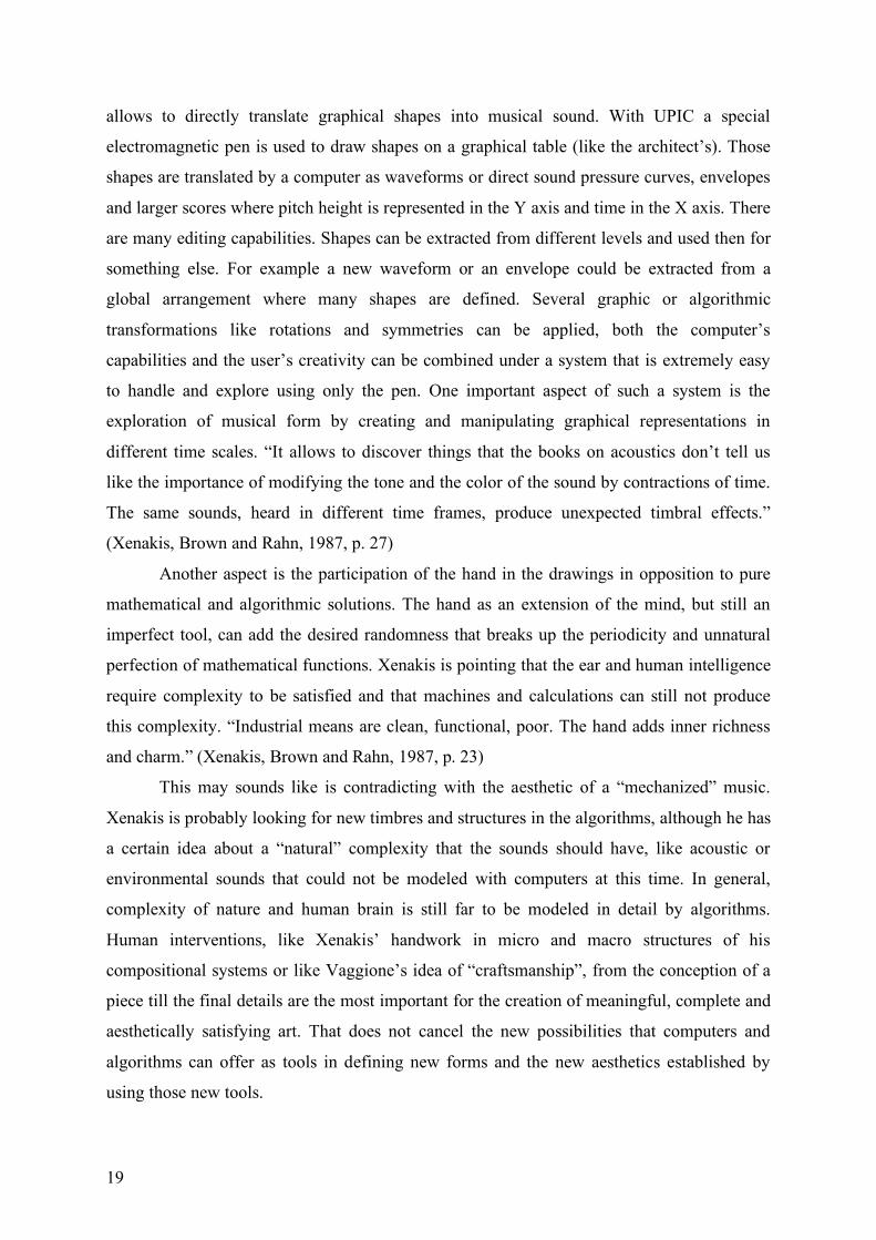
Finally the most important aspect of the UPIC is its intuitive use in real time.

Everybody can use it, doesn’t have to be a composer or a computer specialist, even kids. We

can associate our actions, as we are drawing shapes, with the resulting sound in real time. We

can correct what we don’t like, we can play with time, we can search for new timbres and

instruments, by drawing and listening back, without having to know the complicated

procedures that are taking part in the computer program itself. In this way Xenakis is trying

to propose a new relationship with music, where solfège and music theory knowledge or any

ability to play a physical instrument is not required. With the use of computer and technology

this direct relationship between sound composition and graphical design can be more fun and

can be used for pedagogical purposes as it combines the occupation with mathematics,

geometry, forms and music in a pleasant and creative application.

Figure 2.3: Part of Mycenae-Alpha by Xenakis using the UPIC

The use of graphic representations for shaping musical form is becoming very

common. Envelopes and breakpoint functions are broadly used to express the development of

several musical parameters over time, to define boundary conditions or even to shape spectral

morphologies. An interesting case of shaping musical form is by using tendency masks.

Tendency masks are graphic representations that define the limits of stochastically selected

parameters. They are setting the minimum and maximum of the random values that a

parameter can have and that range varies over time accordingly to the designed shape. James

Tenney has been experimenting with stochastic computer programs. He was trying to add

diversity and “dramatic” development in his forms: “I began to consider what this process of

“shaping” a piece really involved... One question still remained as to the possible usefulness

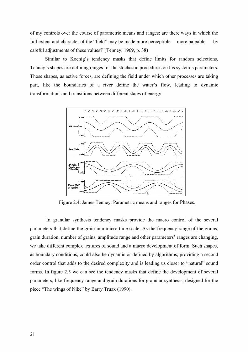
21

of my controls over the course of parametric means and ranges: are there ways in which the

full extent and character of the “field” may be made more perceptible —more palpable — by

careful adjustments of these values?”(Tenney, 1969, p. 38)

Similar to Koenig’s tendency masks that define limits for random selections,

Tenney’s shapes are defining ranges for the stochastic procedures on his system’s parameters.

Those shapes, as active forces, are defining the field under which other processes are taking

part, like the boundaries of a river define the water’s flow, leading to dynamic

transformations and transitions between different states of energy.

Figure 2.4: James Tenney. Parametric means and ranges for Phases.

In granular synthesis tendency masks provide the macro control of the several

parameters that define the grain in a micro time scale. As the frequency range of the grains,

grain duration, number of grains, amplitude range and other parameters’ ranges are changing,

we take different complex textures of sound and a macro development of form. Such shapes,

as boundary conditions, could also be dynamic or defined by algorithms, providing a second

order control that adds to the desired complexity and is leading us closer to “natural” sound

forms. In figure 2.5 we can see the tendency masks that define the development of several

parameters, like frequency range and grain durations for granular synthesis, designed for the

piece “The wings of Nike” by Barry Truax (1990).

22

Figure 2.5: Barry Truax. Tendency masks for “The Wings of Nike”

Many applications, after UPIC, are dealing with similar concepts of intuitive

exploration of complex sound structures by using graphical representations. With the

development of the wavetable lookup technique, graphical approaches on sound synthesis

started to look very promising. As the computers power is increasing, together with the

software development and their Graphical Users Interfaces (GUI), we can handle and

visualize complex data sets in real time. Multidimensional graphical approaches for sound

generation and control appear. Real or generative topologies are traced in Wave Terrain

Synthesis implementations and three-dimensional trajectories are used to intuitively explore

higher dimensional parameter spaces or spatialize sound objects in 3D surround sound

environments. Geometric visualizations and their transformations are providing tools for the

exploration of timbral or other, still unexplored, areas of sound structures. Such examples are

presented in detail in the next chapter. The creation, navigation and manipulation of three-

dimensional virtual environments can lead to new, creative and intuitive, ways of structuring

sound material and handling complexity in musical applications.

23

3. Multidimensional

Data Sets Musical applications using multidimensional data sets have been developed over the years

both in the fields of algorithmic composition and generative sound synthesis. Information can

be extracted by traversing multi-dimensional topologies generated from many different

concepts. Real maps, mathematically derived surfaces, chaotic maps, video color information

are just some examples of multidimensional data sets and each can imprint its unique qualities

while applied onto several musical processes. Dynamic handling of such data sets is also

possible by changing directly parameters that define the used equations, by visual

manipulations of the represented maps and many more. Computer and software development

allows for creation, representation and manipulation of really complex data sets (for example

using matrices or statistical methods).

Aspects of a method for generating sound signals using multidimensional data sets,

conventionally termed Wave Terrain Synthesis, were a great inspiration and starting point for

this research. Firstly because of the (architectural) beauty of the graphic representations of

the participating algorithms, that need to be realized so to understand the complex procedures

24

that are taking part, and how this leads to a visual approach on exploring complex sound

structures. Secondly, because is a generalized method describing (and expanding) many

different sound synthesis methods depending on the selected functions and their dimensions

and how this understanding can lead to a more generalized approach on exploring and

reconstructing musical forms by taming multidimensional spaces.

3.1 Wave Terrain Sythesis

After some ideas and implementations of translating real world topographical maps into

signals for sound generation, Rich Gold (1979) termed as Wave Terrain a virtual

multidimensional surface that can be used for generating audio waveforms and presented the

“Terrain Reader”. Wave Terrain Synthesis is realized by the combination of two independent

structures for generating sound signals. A trajectory signal (or orbit) and a terrain function.

The trajectory is used to create a ‘path’ of coordinates that are used to read from a function of

n variables f (x1,x2,…xn) , the terrain function. Most implementations use terrain functions of

two variables f (x,y) but such systems can be creatively expanded into more dimensions.

Mitsuhashi in his famous article “Audio Signal Synthesis by Functions of Two Variables”

(1982) names this technique as Two-Variable Function Synthesis. The trajectory curve is

defined by n parametric equations that specify the coordinates (x1,x2…xn) as functions of

time (t) so they control the temporal development of the system. For example coordinates x

and y of a 2-dimensional trajectory curve can be defined by the different equations f(t) and

g(t) respectively. There is an infinite number of combinations of equations that can define the

coordinates of a trajectory. Lines, curves or chaotic functions are just some already

implemented examples. The values of the coordinates (x,y) every moment are used to

calculate solutions of the given terrain function f (x,y) that describe the resulting waveform in

time.

25

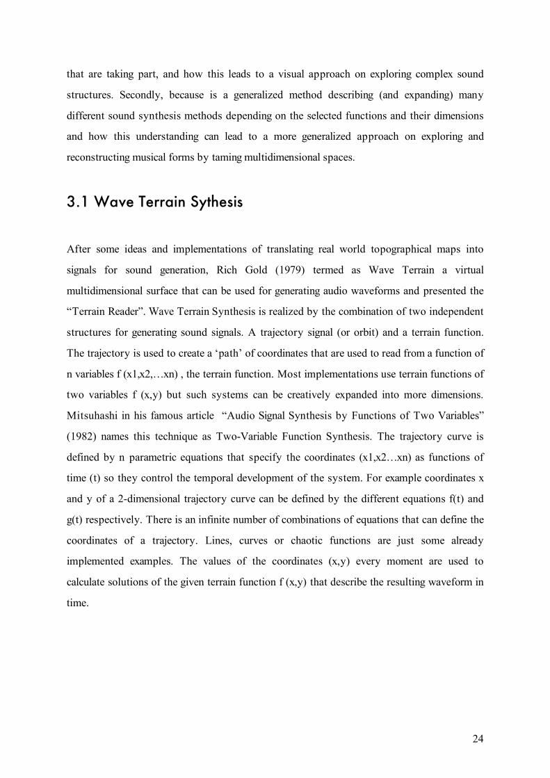
Figure 3.1: An example of Wave Terrain Synthesis

In figure 3.1 we can see an example. A trajectory defined by the parametric equations

x = a sint, y = a sint cost (an Eight Curve) is traversing a surface defined by the equation

f(x,y) = sin(2πx)*cos(2πy).

The resulting signal is defined by the equation f(t) = sin(2π (a sint)) cos(2π (a sint

cost)) with a = 2. We can see that the procedure is similar to Frequency Modulation

Synthesis expanded in more dimensions.

The trajectory function defines the fundamental frequency and temporal development

of the system usually running on high (audible) rates. If it is periodic we perceive a static

spectrum but with even slight modulations of the trajectory we can have dynamic timbral

changes as it reads a different part of the terrain surface. Trajectory functions can be static,

periodic (like various closed curves), quasi-periodic (like spirals), chaotic (like strange

attractors) or even stochastic (like random walks) (James, 2005). Mitsuhashi (1982) suggests

trajectories with both linear and elliptical elements by using the following equations that have

been broadly used for Wave Terrain Synthesis implementations:

26

where fx , fy ,Fx ,Fy are frequencies within the audio range ( 20Hz − 20KHz ) or subaudio

range ( 0 < F < 20Hz,0 < f < 20Hz), φx, φy, ϕx, ϕy are initial phases and Ix(t), Iy(t) behave

as extra modulatable trajectory parameters. While such trajectories lead to more pitched,

periodic and controllable sounds other systems have been implemented using much more

“adventurous" algorithms like Di Scipio’s Functional Iteration Synthesis (2001), where he is

using discrete iterative chaotic functions (see also 2.3), or Choi’s (1994) Chua’s Chaotic

Oscillator digital implementations, where the continuous differential equations of a Chua’s

circuit that display chaotic behavior are used. Chaotic systems usually result to more noisy

and unpredictable sounds with dynamic variation.

Geometric or Affine transformations of the trajectory equations like scaling,

translation and rotation can modify the resulting timbre while we navigate through different

parts of the terrain and by causing phase shifting. Also combinations of equations can be used

for defining the parameters of a trajectory creating additive or multiplicative poly-trajectories

(James 2005) for adding complexity to their temporal development. In this case a periodic

orbit running in an audible rate can be added to another orbit running at a lower rate that

slowly shifts the position of the first.

The terrain function adds complexity to the resulting signal. Approaches to the

terrain function computation include continuous maps and discrete maps. Continuous maps

require an arithmetic approach for constructing the terrain functions using mathematical

models. Algebraic, Trigonometric, Logarithmic/Exponential, Complex, and Composite/Hybrid

mathematical functions (Gold 1978; Mitsuhashi 1982; Mikelson 2000a) have been searched

including fractals, Chebyshev functions and dynamical systems among others. Different

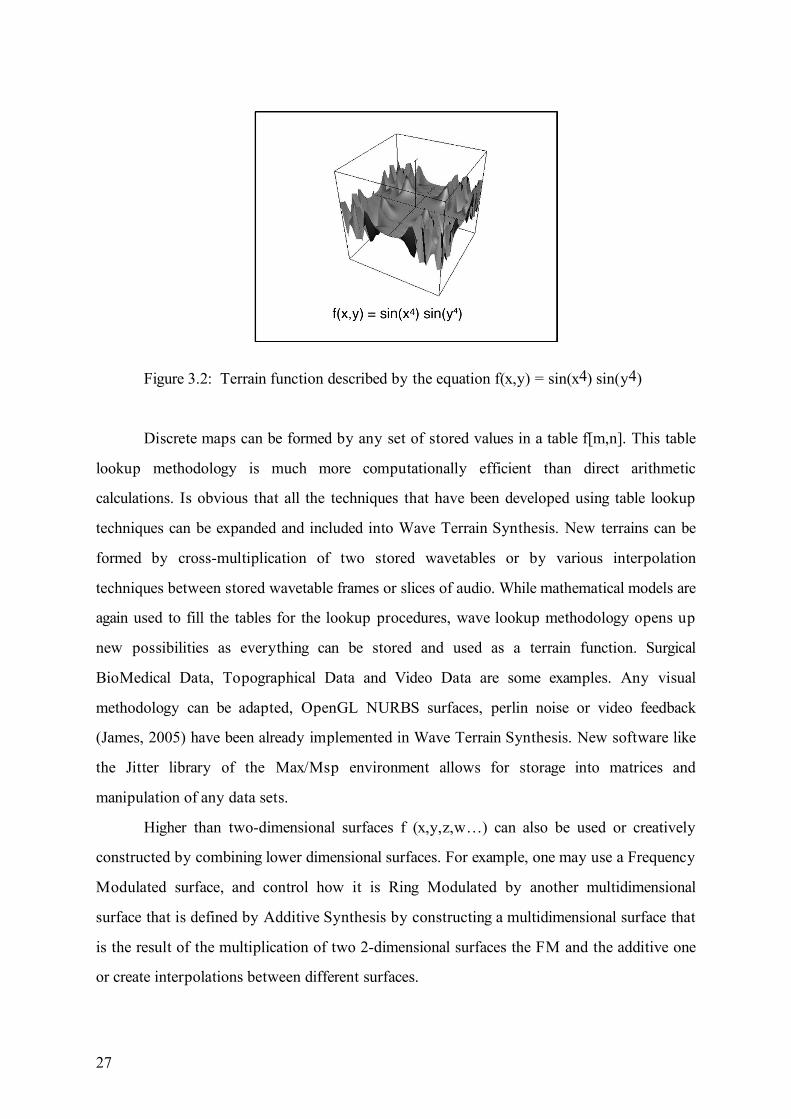
terrain functions imprint their own characteristics on the resulting timbre. In figure 3.2 we can

see a terrain function that is smooth in the center and becoming noisier as we move to the

edges (Mills and de Souza, 1999) given by the equation f(x,y) = sin(x4) sin(y4)

27

Figure 3.2: Terrain function described by the equation f(x,y) = sin(x4) sin(y4)

Discrete maps can be formed by any set of stored values in a table f[m,n]. This table

lookup methodology is much more computationally efficient than direct arithmetic

calculations. Is obvious that all the techniques that have been developed using table lookup

techniques can be expanded and included into Wave Terrain Synthesis. New terrains can be

formed by cross-multiplication of two stored wavetables or by various interpolation

techniques between stored wavetable frames or slices of audio. While mathematical models are

again used to fill the tables for the lookup procedures, wave lookup methodology opens up

new possibilities as everything can be stored and used as a terrain function. Surgical

BioMedical Data, Topographical Data and Video Data are some examples. Any visual

methodology can be adapted, OpenGL NURBS surfaces, perlin noise or video feedback

(James, 2005) have been already implemented in Wave Terrain Synthesis. New software like

the Jitter library of the Max/Msp environment allows for storage into matrices and

manipulation of any data sets.

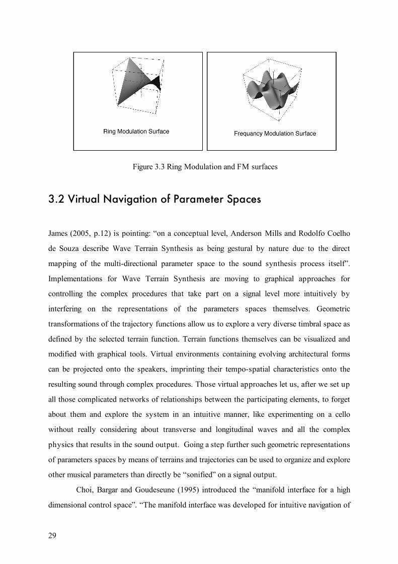
Higher than two-dimensional surfaces f (x,y,z,w…) can also be used or creatively

constructed by combining lower dimensional surfaces. For example, one may use a Frequency

Modulated surface, and control how it is Ring Modulated by another multidimensional

surface that is defined by Additive Synthesis by constructing a multidimensional surface that

is the result of the multiplication of two 2-dimensional surfaces the FM and the additive one

or create interpolations between different surfaces.

28

Dynamic evolution of the terrain functions is also possible for adding even more

complexity and temporal development to the resulting sounds. This can be done by altering

parameters of the surface equations or choosing dynamical systems as surfaces, by visual

effects when we are dealing with video data, “sculpting” surfaces with the use of external

sensors and many other ways. An approach where the timbral evolution is not controlled by

the transformations of the trajectory function but by time varying terrain functions is Scanned

Synthesis developed by Bill Verplank, Max Mathews and Rob Shaw at Interval Research

between 1998 and 2000 (Boulanger, 2000). In Scanned Synthesis a dynamical wavetable that

describes a slowly (in haptic rates) evolving system or a physical model, like a slowly

vibrating string or a two dimensional surface obeying the wave equation, is scanned

periodically by a trajectory function. The pitch is defined by the scanning trajectory when the

evolving timbre of the resulting sounds is defined by the scanned dynamic system. The first

scanned synthesis implementations were realized with Paris Smaragdis’ opcodes for Csound

in 1999. Mikelson (2000b) also implemented dynamically modulated surfaces for terrain

mapping systems in Csound.

We can see that the possibilities for combining all these elements are endless. Using a

different methodology, equations and dimensions, “both the concept as well as the results of

this technique seem to have hovered somewhere within the realms of Wavetable Lookup,

Wavetable Interpolation and Vector Synthesis, Amplitude Modulation Synthesis, Frequency

Modulation Synthesis, Ring Modulation Synthesis, Waveshaping and Distortion Synthesis,

Additive Synthesis, Functional Iteration Synthesis, Scanned Synthesis” (James, 2005, p. 12)

and more.

29

Figure 3.3 Ring Modulation and FM surfaces

3.2 Virtual Navigation of Parameter Spaces

James (2005, p.12) is pointing: “on a conceptual level, Anderson Mills and Rodolfo Coelho

de Souza describe Wave Terrain Synthesis as being gestural by nature due to the direct

mapping of the multi-directional parameter space to the sound synthesis process itself”.

Implementations for Wave Terrain Synthesis are moving to graphical approaches for

controlling the complex procedures that take part on a signal level more intuitively by

interfering on the representations of the parameters spaces themselves. Geometric

transformations of the trajectory functions allow us to explore a very diverse timbral space as

defined by the selected terrain function. Terrain functions themselves can be visualized and

modified with graphical tools. Virtual environments containing evolving architectural forms

can be projected onto the speakers, imprinting their tempo-spatial characteristics onto the

resulting sound through complex procedures. Those virtual approaches let us, after we set up

all those complicated networks of relationships between the participating elements, to forget

about them and explore the system in an intuitive manner, like experimenting on a cello

without really considering about transverse and longitudinal waves and all the complex

physics that results in the sound output. Going a step further such geometric representations

of parameters spaces by means of terrains and trajectories can be used to organize and explore

other musical parameters than directly be “sonified” on a signal output.

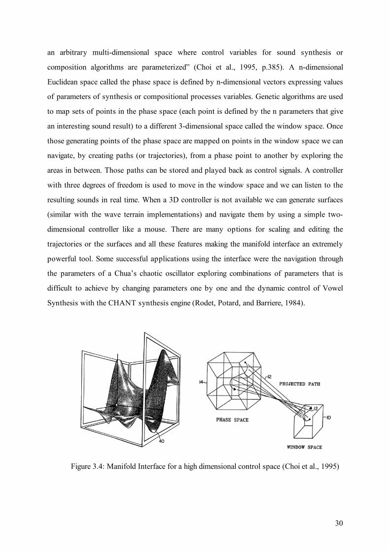
Choi, Bargar and Goudeseune (1995) introduced the “manifold interface for a high

dimensional control space”. “The manifold interface was developed for intuitive navigation of

30

an arbitrary multi-dimensional space where control variables for sound synthesis or

composition algorithms are parameterized” (Choi et al., 1995, p.385). A n-dimensional

Euclidean space called the phase space is defined by n-dimensional vectors expressing values

of parameters of synthesis or compositional processes variables. Genetic algorithms are used

to map sets of points in the phase space (each point is defined by the n parameters that give

an interesting sound result) to a different 3-dimensional space called the window space. Once

those generating points of the phase space are mapped on points in the window space we can

navigate, by creating paths (or trajectories), from a phase point to another by exploring the

areas in between. Those paths can be stored and played back as control signals. A controller

with three degrees of freedom is used to move in the window space and we can listen to the

resulting sounds in real time. When a 3D controller is not available we can generate surfaces

(similar with the wave terrain implementations) and navigate them by using a simple two-

dimensional controller like a mouse. There are many options for scaling and editing the

trajectories or the surfaces and all these features making the manifold interface an extremely

powerful tool. Some successful applications using the interface were the navigation through

the parameters of a Chua’s chaotic oscillator exploring combinations of parameters that is

difficult to achieve by changing parameters one by one and the dynamic control of Vowel

Synthesis with the CHANT synthesis engine (Rodet, Potard, and Barriere, 1984).

Figure 3.4: Manifold Interface for a high dimensional control space (Choi et al., 1995)

31

There are two interesting points described in this work that should be mentioned. The

first is the feedback process when dealing with a musical instrument and the realization of the

“asymptotic” character of the signals transmitted to the instruments from our physical

actions (we could say way of excitation) and the signals arriving to our cognitive system as

transmitted by the instrument through sound waves. We “intuitively” learn how the

instrument responds to different ways of excitation and can associate different actions with

different results without thinking about the complex processes that are taking part while the

sound is produced as previously described. The manifold interface and many more recent

implementations succeed this “intuitive” control of complex electronic instruments by

dimensionality reduction and machine learning algorithms as mapping techniques (mapping

techniques are analyzed in following chapters). The second point to be mentioned is the need

for graphical representations when composing with electronic instruments for helping us to

create our imagined forms. “The breakpoint function has become the composer’s

indispensable visual and conceptual partner” (Choi et al., 1995, p.385). However the linear

connection between a geometric dimension of a break point function and the associated

musical parameter is criticized as it gives many times predictable or uninteresting results. The

manifold approach works also here as many breakpoint functions and non-linearities between

parameters and their geometric representations can easily be controlled dynamically. An

intuitive control of complex processes can be achieved as with acoustic instruments.

Numerous other works extend the manifold idea and the Wave Terrain Synthesis

concept to the visualization, control and exploration of multidimensional complex spaces

(Sedes, Courribet and Thiebaut, 2004; Filatriau, Arfib and Couturier, 2006; Thiebaut, Bello

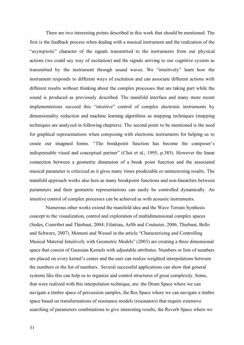
and Schwarz, 2007). Momeni and Wessel in the article “Characterizing and Controlling

Musical Material Intuitively with Geometric Models” (2003) are creating a three dimensional

space that consist of Gaussian Kernels with adjustable attributes. Numbers or lists of numbers

are placed on every kernel’s center and the user can realize weighted interpolations between

the numbers or the list of numbers. Several successful applications can show that general

systems like this can help us to organize and control structures of great complexity. Some,

that were realized with this interpolation technique, are: the Drum Space where we can

navigate a timbre space of percussion samples, the Res Space where we can navigate a timbre

space based on transformations of resonance models (resonators) that require extensive

searching of parameters combinations to give interesting results, the Reverb Space where we

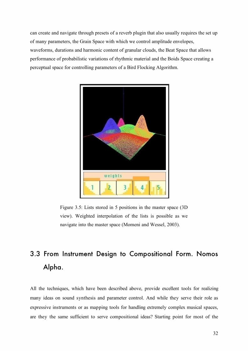
32

can create and navigate through presets of a reverb plugin that also usually requires the set up

of many parameters, the Grain Space with which we control amplitude envelopes,

waveforms, durations and harmonic content of granular clouds, the Beat Space that allows

performance of probabilistic variations of rhythmic material and the Boids Space creating a

perceptual space for controlling parameters of a Bird Flocking Algorithm.

Figure 3.5: Lists stored in 5 positions in the master space (3D

view). Weighted interpolation of the lists is possible as we

navigate into the master space (Momeni and Wessel, 2003).

3.3 From Instrument Design to Compositional Form. Nomos

Alpha.

All the techniques, which have been described above, provide excellent tools for realizing

many ideas on sound synthesis and parameter control. And while they serve their role as

expressive instruments or as mapping tools for handling extremely complex musical spaces,

are they the same sufficient to serve compositional ideas? Starting point for most of the

33

previously described implementations is a controller, a mouse, a keyboard, faders or more

advanced systems, although all controlled by humans and somehow limited to a haptic rate

and to human limitations. This is probably enough for a live performance with a system -

instrument, where features like the instrument’s response to the performer’s actions are

important, but when composing a higher level of structures is essential. Another layer could

work as a replacement for the human gesture, providing organized patterns and their

transformations under new concepts. Concepts that can also derive from algorithms. New

morphologies can be traced in all possible time scales and in multiple layers, imprinting their

special characteristics to the resulting musical structures.

A nice example of creating musical patterns from organized transformations of three

dimensional spatial arrangements (or architectural representations) is Nomos Alpha, a piece

by Iannis Xenakis that could be considered as a composition with multidimensional data sets.

Nomos Alpha for solo cello expresses what Xenakis is describing in Formalized Music as

symbolic music, a compositional method where all the musical relationships are built using

sets theory, abstract algebra and mathematical logic.

“But everything in pure determinism or in less pure determinism is subjected to the

fundamental operational laws of logic, which were disentangled by mathematical

thought under the title of general algebra. These laws operate in isolated states or on

sets of elements with the aid of operations, the most primitive of which are the union,

the intersection and the negation. Equivalence, implication, and quantifications are

elementary relations from which all current science can be constructed.

Music, then, may be defined as an organization of these elementary operations

and relations between sonic entities or between functions of sonic entities” (Xenakis

1992, p.4)

As it is already mentioned in 2.3, Xenakis is proposing a reconstruction of the basic

ideas in musical composition as much possible ex nihilo by using modern axiomatic methods

meaning his scale types or “sieves” and the formation of vector spaces of musical parameters

that are developing under certain rules.

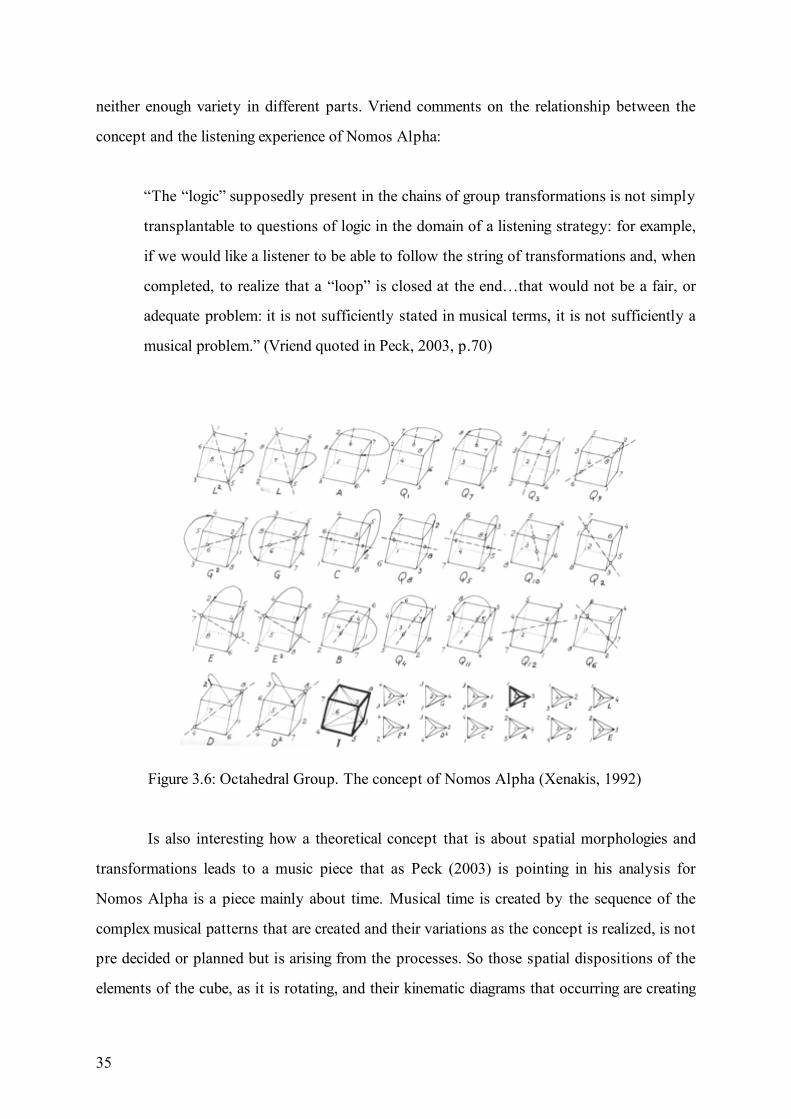
Nomos Alpha is based on the theory of groups of transformations. All musical

34

parameters are described as vector spaces and various mathematical, logical and algebraic,

expressions are defining the laws and the relationships that connect those elements and define

the several musical parts in many ways. Here the 24-element octahedral group isomorphic to

the rotations of a cube determines the musical parts. De Lio separates the processes in

Nomos Alpha in two layers “On level I eight distinct elements are defined for each parameter

and then used to articulate the permutation schemes. In contrast, on level II the sonic

elements seem tied to one another within an unbroken temporal/spatial continuum” (De Lio

quoted in Peck, 2003, p.70).

Analyzing the mathematical and musical elements of all sections and layers of Nomos

Alpha would require a whole book. However we can make some more general thoughts about

the concept, the processes and the musical result. The starting point for all calculations, the

octahedral group of rigid motions (rotational symmetry group) which maps the eight vertices

of a cube, could be considered the main “concept” or “basic structure” and could also be

considered an “architectural” concept as it deals with a geometric object, therefore with

properties of a three dimensional space. All the complex network of laws and connections

between the cube and the vectors which contain the several musical parameters’ symbols

could be considered just mapping functions, that certainly define also compositional decisions

and they are integrated part of the system. When a rotation of the cube is actualized, the

information travels to the related part of this complicated system and a specific output is

realized, a musical form is born. The result doesn’t directly represent the initial concept. The

concept, we could name it virtual according to Kwinter’s theory, sets this complex body of

established relations on motion producing the final result, vectors of musical symbols that are

occupying a different space. The laws are carefully designed so the result will have meaningful

musical properties and forms while the initial idea belongs to a different world; it is expressing

properties of our experienced three-dimensional space. Projections of points in space, as the

cube is rotating in different ways, are leaving traces with characteristic morphologies. Every

differentiation from one point to another and from one moment to another, sometimes taken

as a continuous path and sometimes at selected fragments, is causing irreversible

transformations to the musical parameters, therefore is producing musical form. Mapping

choices are very important for creating complexity and transferring the morphologies of the

concept to the musical output as one to one connections do not guarantee musical meaning,

35

neither enough variety in different parts. Vriend comments on the relationship between the

concept and the listening experience of Nomos Alpha:

“The “logic” supposedly present in the chains of group transformations is not simply

transplantable to questions of logic in the domain of a listening strategy: for example,

if we would like a listener to be able to follow the string of transformations and, when

completed, to realize that a “loop” is closed at the end…that would not be a fair, or

adequate problem: it is not sufficiently stated in musical terms, it is not sufficiently a

musical problem.” (Vriend quoted in Peck, 2003, p.70)

Figure 3.6: Octahedral Group. The concept of Nomos Alpha (Xenakis, 1992)

Is also interesting how a theoretical concept that is about spatial morphologies and

transformations leads to a music piece that as Peck (2003) is pointing in his analysis for

Nomos Alpha is a piece mainly about time. Musical time is created by the sequence of the

complex musical patterns that are created and their variations as the concept is realized, is not

pre decided or planned but is arising from the processes. So those spatial dispositions of the

elements of the cube, as it is rotating, and their kinematic diagrams that occurring are creating

36

differentiations or variations of the musical patterns thus musical time and form. Real time

can be the morphological order in which forms of the different parts are shaped and then

placed the one after the other.

The precision with which all the compositional system of Nomos Alpha is designed,

the strict mathematical laws and calculations for every participating element and the

representation of musical symbols as vectors makes it completely “computerized” and that is

leading to a unique aesthetic result. It could also be mentioned that Nomos Alpha and its

mechanical construction constitutes a challenge for the performers as it is technically very

difficult and includes various extended cello techniques.

This process of composing Nomos Alpha is reminiscent of building the manifold

interface. A familiar virtual three-dimensional space where spatial properties are mapped

through complex procedures to higher dimensional vectors containing representations of

musical parameters. But Nomos Alpha proposes also an initial concept of using this three

dimensional space in an organized way, than “intuitively” navigating into it, limiting the

infinite possibilities of the resulting output and forcing it to be realized under a compositional

idea and quite a “magical” one as every full rotation of the cube places the 8 vertices in their

initial position although a different path is followed. The compositional approach of Nomos

Alpha could also be associated with the Wave Terrain Synthesis technique where affine

transformations of the trajectories’ representations are producing perpetual timbral variations

and transformations. The virtual element of the cube could be replaced with a new, even

dynamic, set of points in 3D space. Those points could be mapped to many musical

parameters by using several, similar to the manifold interface, constructions and affine or

other transformations could be applied on those virtual arrangements to produce different

patterns, variations and transformations. Extending the Wave Terrain Synthesis idea from a

sound synthesis technique to a compositional method we could create dynamic and complex

musical structures, taking advantage of the special morphologies of each trajectory as well as

of the intuitive way to create variations of those structures, by using graphical manipulations.

Trajectories, acting in different time scales, can be a replacement or an extension for musical

gestures and define generative “scores” as basic structures for producing musical form.

37

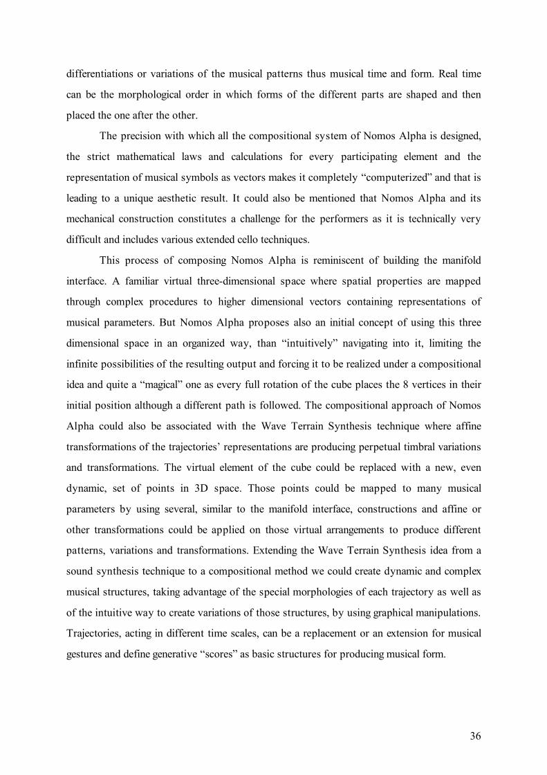
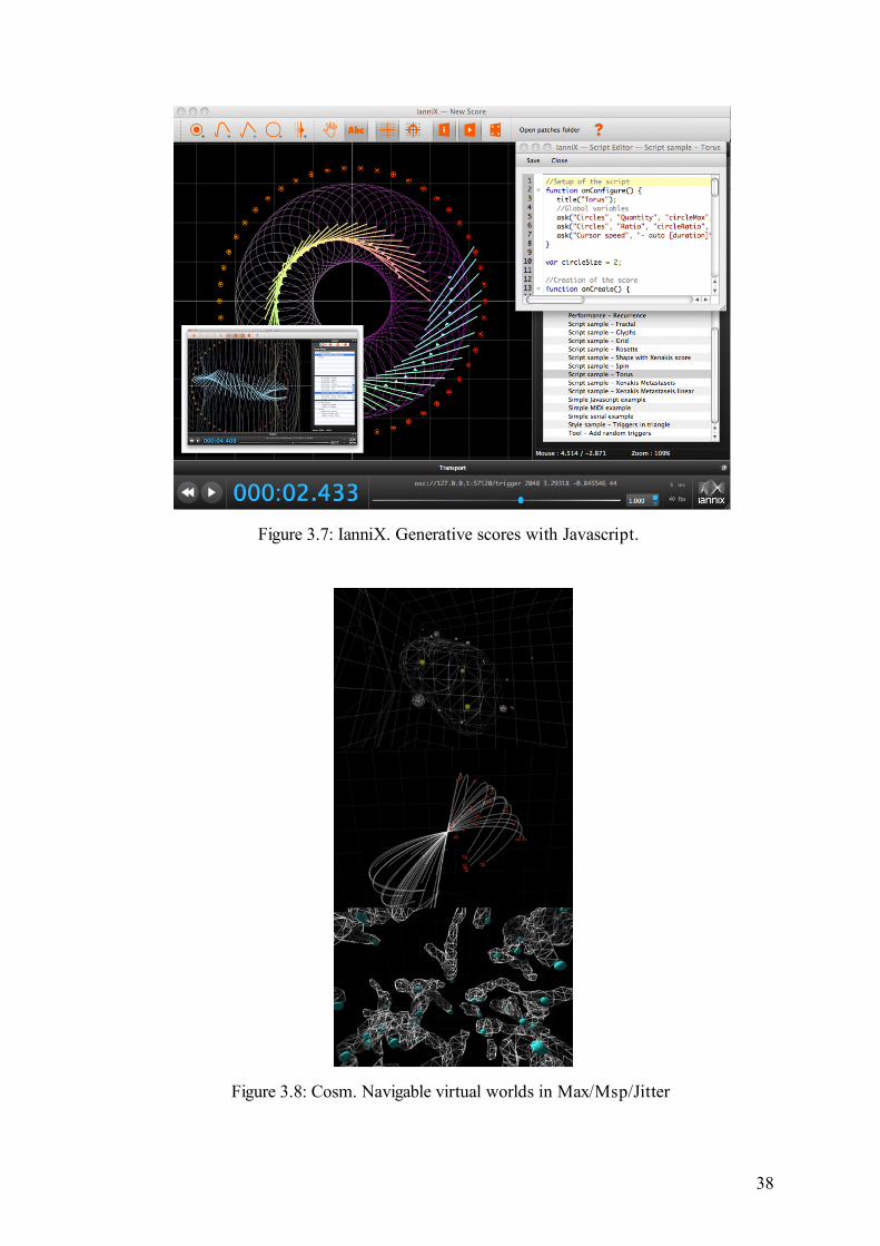
3.4 Generative scores and worlds

IanniX and Cosm are two recent applications where multidimensional virtual environments

can be constructed graphically or algorithmically and navigated in order to create complex

sonic structures and spatial sound experiences.

IanniX (www.iannix.org) is a graphical open source sequencer, inspired by Iannis

Xenakis works. In Iannix we can define “triggers”, as momentary events in space, draw

“curves”, as continuous points in space that define a trajectory, and use “cursors”, elements

that move into space and activate the triggers or read the continuous values of the curves. A

graphical interface allows the visualization and the control of the defined elements. There are

several tools for the design of trajectories; we can use straight lines, polygons, circles and

ellipsis, Bézier curves, text characters and more. Different cursors can be assigned on curves

or trigger momentary events with separate speed adjustments. A general speed of the score

acts like a velocity factor for all cursors so we can accelerate or decelerate the score. One of

the interesting functions of IanniX is the possibility of creating generative scores using

Javascript. In this way really complex trajectory structures can be designed in a relatively

simple manner. Iannix syncs via Open Sound Control (OSC) events and curves to any real-

time environment like Max/Msp, Super Collider or Processing. The created trajectories can

define basic structures for sound synthesis applications but also for video, light shows and

more.

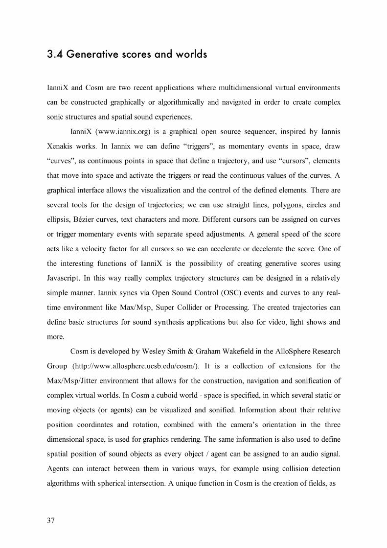
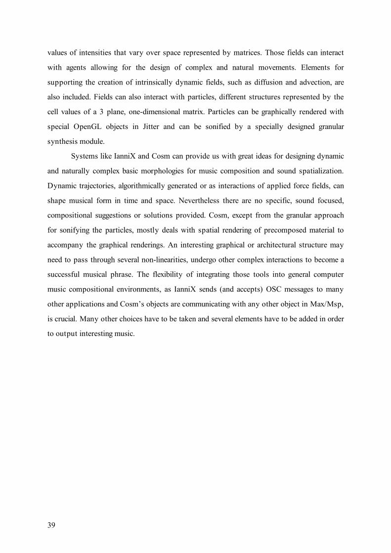
Cosm is developed by Wesley Smith & Graham Wakefield in the AlloSphere Research

Group (http://www.allosphere.ucsb.edu/cosm/). It is a collection of extensions for the

Max/Msp/Jitter environment that allows for the construction, navigation and sonification of

complex virtual worlds. In Cosm a cuboid world - space is specified, in which several static or

moving objects (or agents) can be visualized and sonified. Information about their relative

position coordinates and rotation, combined with the camera’s orientation in the three

dimensional space, is used for graphics rendering. The same information is also used to define

spatial position of sound objects as every object / agent can be assigned to an audio signal.

Agents can interact between them in various ways, for example using collision detection

algorithms with spherical intersection. A unique function in Cosm is the creation of fields, as

38

Figure 3.7: IanniX. Generative scores with Javascript.

Figure 3.8: Cosm. Navigable virtual worlds in Max/Msp/Jitter

39

values of intensities that vary over space represented by matrices. Those fields can interact

with agents allowing for the design of complex and natural movements. Elements for

supporting the creation of intrinsically dynamic fields, such as diffusion and advection, are

also included. Fields can also interact with particles, different structures represented by the

cell values of a 3 plane, one-dimensional matrix. Particles can be graphically rendered with

special OpenGL objects in Jitter and can be sonified by a specially designed granular

synthesis module.

Systems like IanniX and Cosm can provide us with great ideas for designing dynamic

and naturally complex basic morphologies for music composition and sound spatialization.

Dynamic trajectories, algorithmically generated or as interactions of applied force fields, can

shape musical form in time and space. Nevertheless there are no specific, sound focused,

compositional suggestions or solutions provided. Cosm, except from the granular approach

for sonifying the particles, mostly deals with spatial rendering of precomposed material to

accompany the graphical renderings. An interesting graphical or architectural structure may

need to pass through several non-linearities, undergo other complex interactions to become a

successful musical phrase. The flexibility of integrating those tools into general computer

music compositional environments, as IanniX sends (and accepts) OSC messages to many

other applications and Cosm’s objects are communicating with any other object in Max/Msp,

is crucial. Many other choices have to be taken and several elements have to be added in order

to output interesting music.

40

4. Mapping

4.1 Composing Mappings

4.1.1 General

“Music is not dependent on logical constructs unverified by physical experience.

Composers, especially those using computers, have learned—sometimes painfully—

that the formal rigor of a generative function does not guarantee by itself the musical

coherence of a result. Music cannot be confused with (or reduced to) a formalized

discipline” (Vaggione, 2001, p.54)

Vaggione is searching the role of the computer and the algorithms in music composition

processes. The computer and the algorithms as tools, serve their role in a chain of complex

interactions where the composer’s choices, combinations, programming decisions and manual

operations are also inextricably connected. Koenig (1985) refers to interpretation, the

evaluation of an algorithmically generated score by the composer, from the elaboration and

revision of its numbers and symbols to the execution and hearing of the musical output. The

evaluation of the initial concept and compositional ideas, before any calculation has been

made, is integral part of the same interpretation and affects the whole complex system of a

compositional process. A composer can choose algorithms and operations that will serve his

41

concepts and aesthetic choices (that can include the selection of sound sources, instruments or

sound synthesis techniques). Although the transfer from an algorithmic concept to a musical

output may require special treatment, the passage through many other processes, in order to

create a meaningful piece of music. We saw how Nomos Alpha, even if it is all calculated and

“mechanized”, is based on the invention of algorithms (like the sieves) that deal with musical

properties of the symbols and ensure a musical meaning as the basic structuring concept of

the cube belongs to a non musical space.

There are endless possibilities and combinations of connecting information derived

from algorithmic processes or some non-musical concept to musical parameters and they are

depended on the composer’s creativity and taste. While in instrumental composition

(algorithmic or not) those connections are reflected by the composer’s imagination (and

maybe calculations) straight on to the score or the instructions (distribution of instruments,

excitation techniques, pitch - duration arrangements), in computer music have to be explicitly

and precisely defined so to become code. All imagined interconnections from the “virtual”

design to the emerging output have to be parameterized and clearly defined.

When we deal with the translation of form as spatial configurations to musical form

we have to be careful as a direct linear connection can be out of musical context. We saw how

in programs like IanniX a direct and linear translation of the complex trajectories to musical

parameters (like frequency) can be proved to be musically uninteresting. In musical software

design, especially with the development of multitouch surfaces and tablets / smart phones

technologies, one can find plenty of sound applications using multidimensional “composers” -

sequencers. And while most of them may look impressive and provide new creative ways to

organize musical material the sound results (or at least those demonstrated) usually lack of

complexity and expressiveness. Simple pitch and duration connections to vertical and

horizontal dispositions may give interesting results, depending on the design and control of

the interface but they are not going far from the traditional approach in music with “lattice”

structure of quantized pitch, duration and intensity values. The desired complexity and

expressiveness is of course a combination of the control interface design and the synthesis

model itself (and both are compositional choices) so the question is how we can connect

multidimensional control data with complex sound synthesis parameter values. How

formalized information within our familiar fixed three-dimensional space can be used to

42

explore and reform higher (or even lower) dimensional spaces - complex bodies with sonic

characteristics.

4.1.2 Mapping and Interactivity

Mapping, as used in the computer music research field, involves “the liaison or

correspondence between control parameters and sound synthesis parameters” (Hunt,

Wanderley and Kirk, 2000, p.209), the connection between gestures, or structures and audible

results in a musical performance or composition.

A lot of investigation concerning mapping definitions and techniques has been done

mostly for electronic instrument design where the relationships of input gestural data from

the performer and the output sound have to be established. The simple “one to one” mapping

from faders to musical parameters is not sufficient as more complicated control systems and

sound synthesis modules that require the simultaneous control of a large amount of

parameters, are introduced. Software instruments with different control systems (from visual

interfaces to various sensors and human gesture capturing systems), virtual performers -

improvisors that autonomously respond to physical performer’s gestures or environmental

conditions changes and many more, all need a well designed mapping system that define each

instrument’s unique behavior, responsiveness and flexibility. As in acoustic instruments the

human control signals are exciting complex and nonlinear processes on the body of the

instrument, in computer systems an action can trigger many complicated procedures and

affect many parameters at the same time in order to create interesting sounds. Mostly

connected with human - machine interaction investigation, mapping algorithms referred as

‘human and machine agency’ (Paine, 2002) or ‘behavioral objects’ (Bown, Eldridge and Mc

Cormack, 2009). With the goal of giving to software instruments variation and

unpredictability, dynamic systems work as “agents” causing reactions to performers actions.

In the article ‘Understanding Interaction in Contemporary Digital Music: From Instruments

to Behavioral Objects’ (Bown et al. 2009) the potential of interactive systems to facilitate the

creation of dynamic compositional sonic architectures through performance and improvisation

is explored. Some examples of using advanced mapping techniques for interactive instruments

design are: Blackwell and Young’s (2005) live algorithms that reproduce particular

characteristics of human improvisation and can collaborate actively with human performers in

43

real-time performance without a human operator, Di Scipio’s Audible EcoSystemic Interface

(AESI) (2003), that uses cybernetics principles of a bio-ecological kind (energy exchange,

structural closure, organizational openness, system/ external environment coupling) in the

design of signal processing interfaces and Miroslav Spasov’s ENACTIVE (2011), a program

converting a performer/composer’s expressive sonic and kinetic patterns into continuous

variables for driving sound synthesis and processing in real-time by using mapping algorithms

empowered by the iterative equations which generate chaotic attractors.

“Mapping has come to refer to many aspects of the physical gesture-to-sound chain

of control – from signal conditioning to perceptual and cognitive issues related to

causality and expectation in performance.” (Van Nort and Wanderley, 2007, p. 379)

Bown, Eldridge and Mc Cormack (2009) refer to the “acoustic paradigm” to categorize

digital musical systems according to Winkler. Interactive relationships are explored between

the conducted classical orchestra, the string quartet, the traditional jazz combo and a free

improvisation ensemble. These models draw on the established roles of performer,

composition and instrument in performance and use them to signify different modes of

interaction. Continuums are drawn out between unidirectional control and mutual influence,

fixed composition and collaborative improvisation. Those modes of interaction can be the

starting point to evolve ‘new modes of thought based on the computer’s unique capabilities’

(Bown et al, 2009). Under this acoustic paradigm and Rowe’s dichotomies of player vs.

Instrument and score-driven vs. performance-driven paradigms, digital systems can be

categorized and analyzed as software instruments, virtual performers and composed

instruments. By studying these categories and their characteristics useful information can be

extracted but the subject of interactivity and human - machine relationship in real time

performance situations is not to be in detail investigated in this research. What is more

important for realizing algorithmic design for music, is the mapping as a compositional

feature, a field not so broadly investigated as it can be too personal or too general. And while

the borders between those different categories may be blurred under every designer’s personal

choices, the term composed instruments, as systems that merge compositional features and

instruments in a single object, describes better the approaches that are presented and

44

constructed in this work.

4.1.3 Mapping and Composition. Composed Instruments

In algorithmic composition mapping is usually embedded in the design of the driving

algorithms and the musical process, realizing the intention of the composer. This is maybe the

reason why mapping procedures are not investigated independently. According to

Doornbusch (2002, p. 145) “mapping in algorithmic composition is different from mapping in

instrument design because composition is a process of planning and instruments are for

realtime music production”. Nevertheless realtime or dynamic manipulations of the initial

algorithms - structure is not to be excluded from the compositional process. The action /

perception feedback loop that real time computer systems offer can be an important element

for experimenting on sound forms. He also refers to the meaning of musical gesture as the

starting point for a composition, separating it from physical gestures. Musical gesture is a

planned change of musical parameters. “A compositional gesture is the underlying

conception, structure and planning of the musical gesture. As such, a compositional gesture

can be a kind of abstraction of a musical gesture or a group of musical gestures. Thus

compositional gestures can be directly related to (possibly complex) musical gestures,

possibly as an abstraction” (Doornbusch, 2002, p. 145). So mapping is required for

connecting this ‘conceptual domain’ of organized musical gestures to musical parameters.

Different data sets as sonification of formal or mathematical concepts, Markov chains and

many more are excluded from ‘gestures’ revealing the difficulty of generalizing mapping

systems for algorithmic composition. This ‘conceptual domain’ can be integrated in the

‘virtual’. As it has been previously mentioned, gestures can be considered all kinds of

spatiotemporal differentiations in all possible time scales. Then mapping is the technique of

connecting two spaces with different dimensions, the virtual where the conceptual domain is

expressed in a certain x-dimensional space in time, and the actual - soundspace where a y-

dimensional space is created by all the different parameters that define it. Gestures or

trajectories can dynamically form this new space and mapping act as the transfer function in

between.

In composed instruments the sound producing mechanism is decoupled by the control

surface unlike traditional acoustic instruments (Chadabe 2002). Different controllers,

45

generators and the, in between, mapping sections are individual units that can be combined in

any way providing flexible tools for realizing different ideas. This modular approach and the

independence of the different modules allows to the system to be recomposed according to a

new musical intent. The fixed and direct correspondence between the interface and sound

production mechanism is now broken, fact that leads to more open, flexible and complex

systems. Therefore this flexibility requires a more careful design of the different modules and

their interconnections, a common building architecture and general communication standards

have to be established in order to successfully connect and rearrange several modules. Ppooll

(http://ppooll.klingt.org) and the Jamoma modular (Place and Lossius, 2006) are examples of

such systems for the Max/Msp environment. Several modules for data manipulation,

controllers, sound processing and spatialization units can be combined in various structures.

Data and signals can be transferred from one part to another in a creative way. Jamoma

modular contains special designed mapping units that can connect any parameter to another

parameter with additional mathematical functions in between amplifying “behavioral’’

characteristics. Such systems and their special characteristics and structures can be

compositions themselves as they define the starting point of organizing and structuring as

well as realizing musical ideas, according to their special features.

A general mapping model needs to be designed providing flexibility in connecting

complex data and being open for additional “behavioral” features. This flexible design can

“involve several types of machine learning in order to “train” mappings and “induce them out

of interactions” rather than create a priori arbitrary relationships between input and output”

(Salter, Baalman and Moody-Grigsby, 2007). Elements of non - linearity can also interfere,

from square law to chaotic functions and everything we can imagine, distorting, warping and

redesigning the emerging parameter space according to the introduced algorithms in realtime,

adding more dynamic factors for creating new forms that are unfolding in time under certain

“behavioral” aspects. In this way mapping gets his own role as a compositional decision,

rather than just a necessary tool, and becoming art by itself.

46

4.2 Mapping Strategies

Several mapping techniques have been developed over the years. In general mapping strategies

and their implementations are separated in : one-to-one , one-to-many and many-to-one,

depending on the number of control parameters that we have and the number of synthesis

parameters we need to control. Each of those strategies requires a different approach and with

several combinations we can create many - to many mappings. It has been recognized that

such complex mappings are more satisfactory, as a multiparametric control approach models

better the complexity of sound producing mechanisms in acoustic instruments (or natural

sound), than one-to-one mappings (Van Nort and Wanderley, 2006). Mappings can also be

constructed in a way that they are:

• Explicit: Having an analytic description that is precisely

known to the designer.

• Implicit: Based on internal adaptation of a system. (Van Nort and Wanderley, 2006)

Neural networks have been previously used especially for building implicit mapping

systems with unsupervised training capabilities (Cont, Coduys and Henry, 2004). Van Nort

et al. give a mathematical formulation of mapping as a function g between a controller

parameter space ℜn and a sound parameter space ℜm. If the mapping is described by a series

of discrete couples of vectors {Xi, Yi}, where Xi ⊂ ℜn (control parameter space) and Yi ⊂

ℜm (sound parameter space), the mapping can be seen as an interpolation problem, or a

regression problem when the series {Xi, Yi} overdetermines the mapping function with a

factor of uncertainty for each value of the vectors {Xi, Yi} (Van Nort and Wanderley, 2006).

The manifold interface (Choi, Bargar and Goudeseune, 1995) and Momeni and Wessel’s

(2003) models, as they were presented in 3.2, define solutions, under this geometric

interpretation of the problem of mapping. Many other works suggest multi layered mapping

solutions and can be found in the references (Hunt and Kirk, 2000; Van Nort, Wanderley and

47

Depalle, 2004).

Mapping procedures can be also viewed as pattern recognition problems, especially

many-to-few mappings. Common linear and non-linear techniques in statistical and machine

learning methods seem promising for mapping, for example Principal Component Analysis,

Gaussian Mixture Models, Kernel Methods and Support Vector Machines. Though some of

these methods can still be inconvenient for real-time musical applications or they are applied

in a specific type of mapping. A general and modular mapping approach is sought and MnM

toolbox provides an excellent solution.

The MnM ("Mapping is not Music”) toolbox, result of years of investigation into the

complexity of mapping procedures at IRCAM in Paris, consists of a series of Max/Msp

externals and abstractions based on the FTM library and provides practical tools to

implement complex mappings in a relatively intuitive manner (Bevilacqua, Müller and Schnell,

2005). As the FTM library, MnM is freely distributed. In MnM mappings are described as

relatively simple matrix operations.

4.2.1 Mapping with Matrices

A simple mapping operation corresponds to the matrix multiplication:

Y = A*X Eq. 4.1

Where X is considered to be a vector of size n from the controller parameter space, Y

is considered to be a vector of size m from the sound parameter space and A is a m × n

matrix.

A is a n-to-m linear mapping (from ℜn to ℜm). Depending on the length of n

compared to m we can have many-to-few (n ≥ m) or few-to-many (n < m) mappings. A can

be a time - dependent function A(t).

If n ≥ m, A is a projection from the Euclidian space ℜn to a hyperplan in a subspace

ℜm and if m ≥ n, A can be a linear extrapolation of X in a space of higher dimension Y.

The matrix A can be exactly determined by a series of n examples {Xi, Yi}, where 1 ≤

i ≤ n. If the number of example is larger than n, A can be determined by linear regression.

48

With a combination of different matrices more complex mappings can be constructed.

Layered mappings can be defined by series of matrix multiplications (eq 4.2 where the matrix

B can operate in any space),

Y=(A*B*C) *X Eq. 4.2

element by element multiplications can be used (eq 4.3),

Y=(A.*B) *X Eq. 4.3

or any function f can be applied to any element of the matrix(eq 4.4).

Y= [f(aij)]*X Eq. 4.4

With the combination of equations 4.2, 4.3 and 4.4 powerful non-linear mappings can

be designed.

4.2.2 Linear Mapping

The mnm.matmap abstraction (Bevilacqua, Müller and Schnell, 2005), included in the MnM

toolbox, is used as the basic model for realizing general n-to-m multidimensional linear

mappings and as a starting point for constructing more complex non-linear mappings.

The basic matrix multiplication

Y = Ae*Xe Eq. 4.5

(an extension of the equation Y = A*X + B that describes an affine transform) is used, where

Ae is a m × (n+1) matrix (the mapping matrix) and Xe is coming from the initial vector X of

the control space builded as Xe = (x1,…, xn, 1) and has size n+1.

We take k “training examples” sets of existing {Xi, Yi} and create two matrices Xtrain

(of size (n+1)×k formed by concatenating the vectors Xi) and Ytrain (of size m×k formed by

concatenating the vectors Yi).

Using the equation

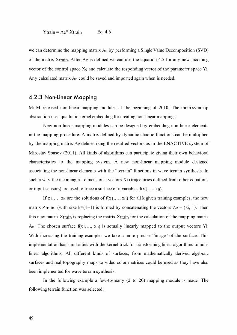
49

Ytrain = Ae* Xtrain Eq. 4.6

we can determine the mapping matrix Ae by performing a Single Value Decomposition (SVD)

of the matrix Xtrain. After Ae is defined we can use the equation 4.5 for any new incoming

vector of the control space Xe and calculate the responding vector of the parameter space Yi.

Any calculated matrix Ae could be saved and imported again when is needed.

4.2.3 Non-Linear Mapping

MnM released non-linear mapping modules at the beginning of 2010. The mnm.svmmap

abstraction uses quadratic kernel embedding for creating non-linear mappings.

New non-linear mapping modules can be designed by embedding non-linear elements

in the mapping procedure. A matrix defined by dynamic chaotic functions can be multiplied

by the mapping matrix Ae delinearizing the resulted vectors as in the ENACTIVE system of

Miroslav Spasov (2011). All kinds of algorithms can participate giving their own behavioral

characteristics to the mapping system. A new non-linear mapping module designed

associating the non-linear elements with the “terrain” functions in wave terrain synthesis. In

such a way the incoming n - dimensional vectors Xi (trajectories defined from other equations

or input sensors) are used to trace a surface of n variables f(x1,…, xn).

If z1,…, zk are the solutions of f(x1,…, xn) for all k given training examples, the new

matrix Ztrain (with size k×(1+1) is formed by concatenating the vectors Ze = (zi, 1). Then

this new matrix Ztrain is replacing the matrix Xtrain for the calculation of the mapping matrix

Ae. The chosen surface f(x1,…, xn) is actually linearly mapped to the output vectors Yi.

With increasing the training examples we take a more precise “image” of the surface. This

implementation has similarities with the kernel trick for transforming linear algorithms to non-

linear algorithms. All different kinds of surfaces, from mathematically derived algebraic

surfaces and real topography maps to video color matrices could be used as they have also

been implemented for wave terrain synthesis.

In the following example a few-to-many (2 to 20) mapping module is made. The

following terrain function was selected:

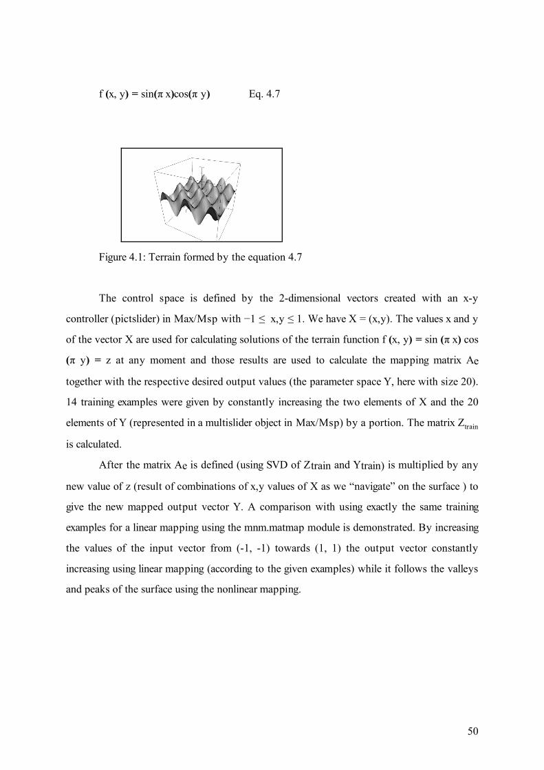
50

f (x, y) = sin(π x)cos(π y) Eq. 4.7

Figure 4.1: Terrain formed by the equation 4.7

The control space is defined by the 2-dimensional vectors created with an x-y

controller (pictslider) in Max/Msp with −1 ≤ x,y ≤ 1. We have X = (x,y). The values x and y

of the vector X are used for calculating solutions of the terrain function f (x, y) = sin (π x) cos

(π y) = z at any moment and those results are used to calculate the mapping matrix Ae

together with the respective desired output values (the parameter space Y, here with size 20).

14 training examples were given by constantly increasing the two elements of X and the 20

elements of Y (represented in a multislider object in Max/Msp) by a portion. The matrix Ztrain

is calculated.

After the matrix Ae is defined (using SVD of Ztrain and Ytrain) is multiplied by any

new value of z (result of combinations of x,y values of X as we “navigate” on the surface ) to

give the new mapped output vector Y. A comparison with using exactly the same training

examples for a linear mapping using the mnm.matmap module is demonstrated. By increasing

the values of the input vector from (-1, -1) towards (1, 1) the output vector constantly

increasing using linear mapping (according to the given examples) while it follows the valleys

and peaks of the surface using the nonlinear mapping.

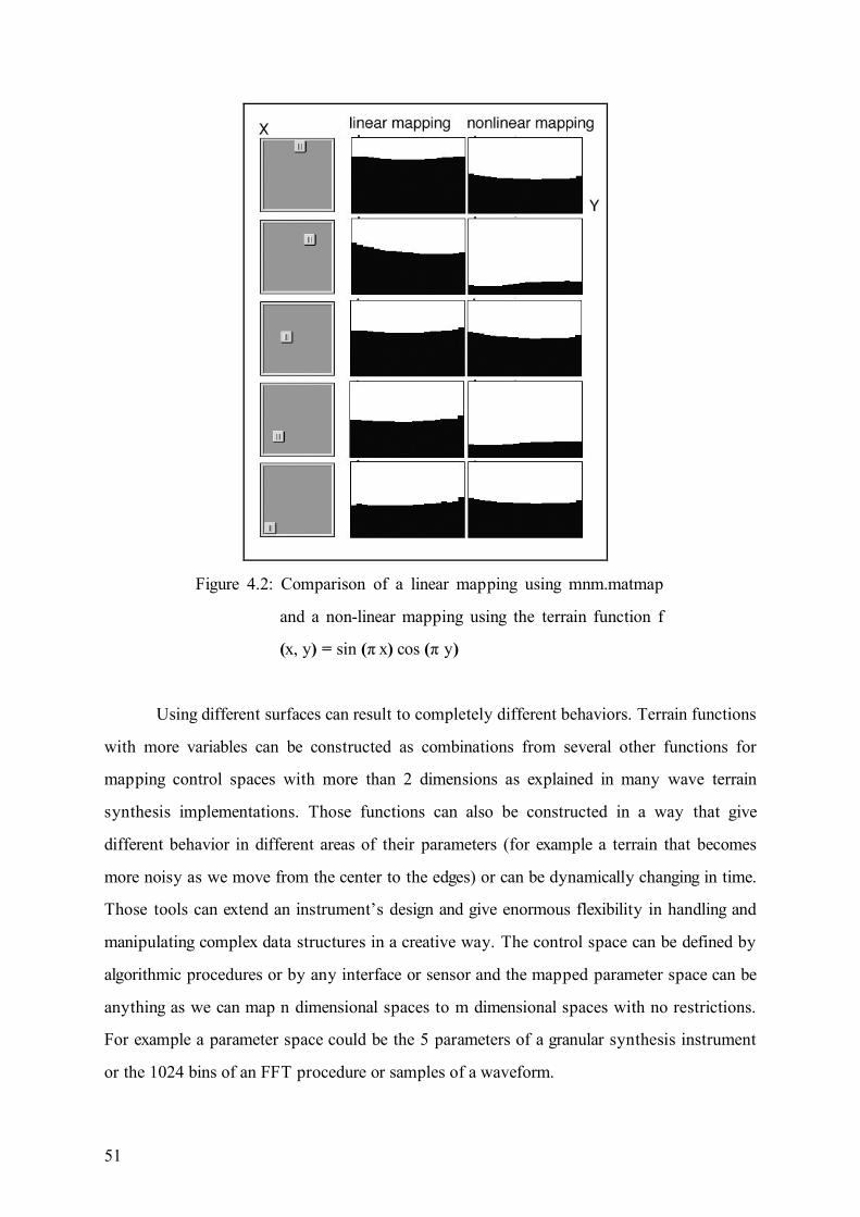
51

Figure 4.2: Comparison of a linear mapping using mnm.matmap

and a non-linear mapping using the terrain function f

(x, y) = sin (π x) cos (π y)

Using different surfaces can result to completely different behaviors. Terrain functions

with more variables can be constructed as combinations from several other functions for

mapping control spaces with more than 2 dimensions as explained in many wave terrain

synthesis implementations. Those functions can also be constructed in a way that give

different behavior in different areas of their parameters (for example a terrain that becomes

more noisy as we move from the center to the edges) or can be dynamically changing in time.

Those tools can extend an instrument’s design and give enormous flexibility in handling and

manipulating complex data structures in a creative way. The control space can be defined by

algorithmic procedures or by any interface or sensor and the mapped parameter space can be

anything as we can map n dimensional spaces to m dimensional spaces with no restrictions.

For example a parameter space could be the 5 parameters of a granular synthesis instrument

or the 1024 bins of an FFT procedure or samples of a waveform.

52

5. Sculpting Space

5.1 Spatial Composition

“I became conscious of a third dimension in the music. I call this phenomenon “sound

projection,” or the feeling given us by certain blocks of sound. Probably I should call

them beams of sound, since the feeling is akin to that aroused by beams of light sent

forth by a powerful searchlight. For the ear - just as for the eye - it gives a sense of

prolongation, a journey into space.” (Varèse, 1936)

Edgar Varèse, already in 1936 expressed the potential for using space as a

compositional parameter interrelated to the rest of musical dimensions like pitch, rhythm and

dynamics. Natural sounds are happening in space therefore the notion of space, reflections,

acoustic properties and spatial positions and movements of sound sources, is always present

in our auditory perception. In instrumental music we can find very old examples of special

space arrangements of instruments or voices. Sound spatialization as a term, includes many

different aspects that could define compositional choices. Positioning of sources, movements

of sounds as choreographies, diffusion of the sound energy, use or simulation of special

acoustics and room ambiences (like reverberation) are some of those aspects (Baalman, 2010).

53

Though, in this work, we are not so much interested in a simulation of existing spaces or

acoustic properties but in formalization of space as structural parameter in musical

composition, and especially in electronic and computer music with the use of new

technologies. Spatialization as a compositional parameter can make more clear dense textures

of sounds, separate simultaneous events into space and make them more perceivable or

animate complicated sonic orbits, adding to the dramatic effect and the immersive experience

of music.

Varèse realized his vision of sound projection with Poème électronique distributed at

the hundreds of speakers of the Philips Pavillion. In 2.1 we saw how Xenakis designed and

used architectural form to project his sounds (in the Phillips Pavilion and later at the

Polytopes), which are traveling on new geometries, resulting to immersive sonic experiences.

The use of technology, microphones, mixing desks and loudspeakers, allowed the design of

imaginary spatial movements beyond the scope of reality. With the development of

computers and hardware, we can create new spatial experiences without having to use a large

amount of loudspeakers or constructed architectural form. New techniques are allowing us to

render spatial movements of many channels of audio and simulate different sound sources in

two-dimensional or three-dimensional speakers’ arrays. Into those several approaches on

spatial sound rendering are included: perception based amplitude panning techniques like

Vector Based Amplitude Panning (VBAP) (Pulkki, 1997) and Distance Based Amplitude

Panning (DBAP) (Lossius, Baltazar and de la Hogue, 2009), techniques that are focusing on a

reconstruction of the sound-field like Wave Field Synthesis (WFS) (Berkhout, de Vries and

Vogel, 1993) and Ambisonics (B-format or Higher Order Ambisonics) (Malham and Myatt,

1995), binaural and transaural techniques or other techniques like Virtual Microphone

Control (ViMiC) (Braasch, 2005).

Each of the above mentioned techniques have different characteristics and maybe is

not suitable for every application. Some of them require a big amount of speakers, some are

working better in hemisphere speakers’ setups (like the VBAP), some require from the

listeners to be in the “sweet spot” and some provide a larger effective area. There are

different assumptions for the nature of the sound sources, the listener’s position and the

placement of loudspeakers. Taking under consideration that a musical work can be played in

different venues, with different available systems, number of loudspeakers and architecture, a

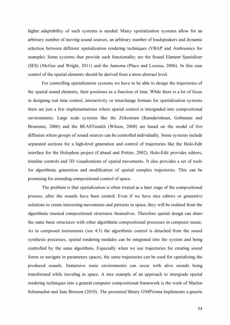
54

higher adaptability of such systems is needed. Many spatialization systems allow for an

arbitrary number of moving sound sources, an arbitrary number of loudspeakers and dynamic

selection between different spatialization rendering techniques (VBAP and Ambisonics for

example). Some systems that provide such functionality are the Sound Element Spatializer

(SES) (McGee and Wright, 2011) and the Jamoma (Place and Lossius, 2006). In this case

control of the spatial elements should be derived from a more abstract level.

For controlling spatialization systems we have to be able to design the trajectories of

the spatial sound elements, their positions as a function of time. While there is a lot of focus

in designing real time control, interactivity or interchange formats for spatialization systems

there are just a few implementations where spatial control is intergraded into compositional

environments. Large scale systems like the Zirkonium (Ramakrishnan, Gobmann and

Brummer, 2006) and the BEASTmulch (Wilson, 2008) are based on the model of live

diffusion where groups of sound sources can be controlled individually. Some systems include

separated sections for a high-level generation and control of trajectories like the Holo-Edit

interface for the Holophon project (Cabaud and Pottier, 2002). Holo-Edit provides editors,

timeline controls and 3D visualizations of spatial movements. It also provides a set of tools

for algorithmic generation and modification of spatial complex trajectories. This can be

promising for extending compositional control of space.

The problem is that spatialization is often treated as a later stage of the compositional

process, after the sounds have been created. Even if we have nice editors or generative

solutions to create interesting movements and patterns in space, they will be isolated from the

algorithmic musical compositional structures themselves. Therefore spatial design can share

the same basic structures with other algorithmic compositional processes in computer music.

As in composed instruments (see 4.3) the algorithmic control is detached from the sound

synthesis processes, spatial rendering modules can be integrated into the system and being

controlled by the same algorithms. Especially when we use trajectories for creating sound

forms or navigate in parameters spaces, the same trajectories can be used for spatializing the

produced sounds. Immersive sonic environments can occur with alive sounds being

transformed while traveling in space. A nice example of an approach to intergrade spatial

rendering techniques into a general computer compositional framework is the work of Marlon

Schumacher and Jean Bresson (2010). The presented library OMPrisma implements a generic

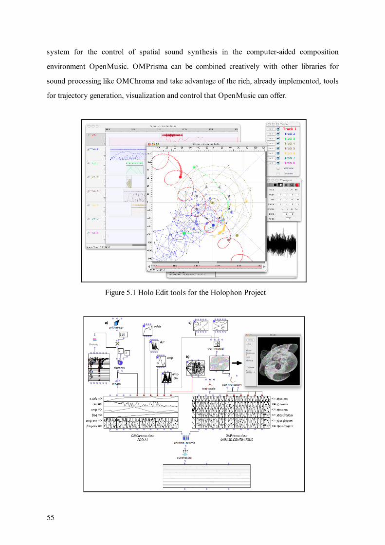
55

system for the control of spatial sound synthesis in the computer-aided composition

environment OpenMusic. OMPrisma can be combined creatively with other libraries for

sound processing like OMChroma and take advantage of the rich, already implemented, tools

for trajectory generation, visualization and control that OpenMusic can offer.

Figure 5.1 Holo Edit tools for the Holophon Project

56

Figure 5.2 Spatial additive synthesis using OMChroma, OMPrisma in OpenMusic

5.2 Spatial Sound Synthesis

In the same way that we can interfere in multiple time scales for sound composition, by using

algorithms and computers, we can introduce spatialization processes also to the micro level of

sounds. Complex spatial morphologies can be created, timbral transformations that occupying

different positions in space or grains of sound where each has his own spatial properties, like

in natural sounds. Schumacher and Bresson (2010) use the term spatial sound synthesis as

sound synthesis processes are extended to the spatial domain.

Examples of spatial sound synthesis can be found in recent researches. Ryan H.

Torchia and Cort Lippe (2004) presented an approach where frequency domain processing is

used to spatialize several spectral components of a sound individually. Extending this

technique of spectral spatialization, the spectral components of a sound can be mapped in

space using the energy of another sound creating a kind of spatial “cross synthesis”. Another

example is Scott Wilson’s Spatial Swarm Granulator (2008) where the spatial position of

individual grains of sound, produced with granular synthesis, is defined by a Reynold’s Boids

algorithm.

DBAP (Lossius, Baltazar and de la Hogue, 2009) can be used as a solution for

dynamic routing of input sources to a spatial layout of effect processes. The way DBAP

works, especially with the introduction of weights for each speaker, which allows for the

distribution of sound sources to specific subsets of speakers, is identical to Momeni and

Wessel’s (2003) system described in 3.2. Instead of assigning loudspeakers positions to

points in space and move in between those points interpolating between amplitude values for

every speaker, we can assign any process. Then we can intuitively navigate into those

parameter spaces and, if combined with DBAP, to their corresponding spatial position. That

helps us to understand the similarities of calculating spatial positions in various rendering

techniques with other sound processing and control procedures. This unifying approach can

lead to the design of interesting spatiotemporal sound arrangements.

Miguel Negrão’s Strategies in Diffused Spatialization (2010) is another great example

57

of using space as a sound synthesis parameter. Negrão names diffuse spatialization:

“the spatialization approaches and techniques that put emphasis on filling the space

with sound, and deal with the sound in space in terms of “volumes” or “areas”, in

such a way that the perception of location becomes extended, and the immersive

qualities are brought to the foreground, making the listener feel that he is inside or

surrounded by one or several sound masses” (Negrão, 2010, p.20)

Negrão associates such arrangements with the feeling of sound produced by natural

phenomena like wind or rain. He built SupaStrings: a network of interconnected physical

modeled strings, with multiple outputs per string, placed in a virtual sound stage, Parameter

Field Synthesis: a grid of stationary sound sources which are using the same synthesis

process and are controlled by time evolving scalar fields and Sine Fields: sine wave oscillators

which are controlled by a frequency scalar field whose frequencies are closely connected to

several points in space. Negrão presented his works using the Wave Field Synthesis system

with impressive results.

In Cosm (see 3.4) spatial positions and movements are connected with the virtual

objects and particles that are participating in the virtual environment using Ambisonics. The

relative position of the object from the camera, and the camera orientation are taken into

account to synthesize directional and distance cues for the spatial rendering. Objects and

particles interact between them or with the created field dynamics creating natural movements

and interactions (like collisions). Especially particles are sonified using granular synthesis.

The same distance filtering settings are used and directional cues are mixed into the same

ambisonic signal busses with the rest of sound/ space objects.

In this research an approach inspired from the Wave Terrain Synthesis technique is

proposed. The idea is to use trajectory functions, as they have been implemented for Wave

Terrain Synthesis, to drive spatial rendering functions in different time scales. Wave Terrain

Synthesis, except a generative sound synthesis method, can also be a transformative technique

for any sound. This kind of spatial Wave Terrain Synthesis is achieved when the trajectory

signals x y and possibly z (if we design three dimensional trajectories) are fed into the spatial

rendering equations. That requires systems for spatialization that work on the signal domain.

In Max/Msp most implementations of spatialization systems, like several VBAP and DBAP

58

objects, are using matrices that are updated in data rates. CICM (Centre de recherche

Informatique et Création Musicale) offers some spatialization objects like vbapan~, ambipan~

and ambicube~ (for two dimensional VBAP spatialization as well as for two and three

dimensional B format Ambisonics respectively) that accept signals as coordinates. There is

not a signal driven three-dimensional VBAP implementation and the ambicube~ works for

predefined number and positions of speakers (a cube setup of 8 speakers). Some quite

successful experiments were made using the vbapan~ object with 8 speakers on a circle. By

using trajectories to control spatial rendering we actually modulate space itself; we use space

as a terrain function to be navigated in low or high rates. We can provide a constant signal in

the spatial rendering system and use the trajectories as a spatial synthesizer. In this case we

loose the extra complexity that the terrain function can give, nevertheless those spatial

oscillators can give a great effect as they occupy large areas around the listeners. We can also

use any sound signal and modulate it into space. Nice results are achieved when we are

speeding up from very low rates to higher rates. The sounds are moving slowly according to

the trajectories’ coordinates, then they start moving faster as well as audible artifacts are

appearing like LFO modulations traveling in space and finally, as we increase further the rate

of the trajectory functions, timbral transformations are occurring with unique spatial

properties. Geometric and other transformations of the trajectories, like rotations and

translations, act on the resulting modulations and timbres while the energy of sound is

transferred to the position in space that the trajectory occupies.

Two dimensional wavetables that are often participating in Wave Terrain Synthesis

implementations, like the 2d.wave~ and jit.peek~ objects in Max/Msp, were also tested.

2d.wave~ is a two-dimensional table lookup object where a given sample is divided into n

rows. One signal X is used to read the samples of the stored waveform and a second signal Y

is defining which row is used for playback. In a similar way, jit.peek~ outputs the values of a

matrix in any position, specified by coordinates given by two signals X and Y. The same

trajectories can be used to simultaneously read the table functions (or terrains) and spatialize

the resulting signals. In this way every sample of the terrain surface is assigned to a particular

position in space and we can navigate onto it in many different ways. The diverse,

multidimensional and exploratory character of Wave Terrain Synthesis can be transferred into

59

musical composition and spatial sound design, opening up new possibilities for creating new

immersive sonic worlds.

60

6. ModTools

6.1 Concept

ModTools is a set of modules implemented in the Max/Msp/Jitter environment. They allow

for generation, visualization, manipulation and navigation of two or three-dimensional

graphical representations of various mathematical models and propose solutions for

multilayered mapping of the extracted information in different parts of complex

compositional systems, including spatial rendering. ViMod is the main module in ModTools.

It provides a host for virtual representations of mathematical models in order to create and

manipulate trajectory functions, as they have been implemented for Wave Terrain Synthesis

and other previously described techniques. Trajectories can be edited and geometrically

transformed in various ways in real time. Multiple “particles” are tracing the trajectory

functions in different time scales. The movement of particles on the trajectory paths can be

considered as the result of complex dynamics. It represents the physics and spatiotemporal

morphology of the trajectory functions. KineMod is another module that extracts information

based on the kinematics and differential geometry of the particles’ movement along the

curves and surfaces of the mathematical models. Position in three dimensions, velocity,

acceleration, curvature and torsion describe the particles’ orbits special morphologies in time

and space and can be used to control any sound parameter. Several linear and non-linear

61

mapping modules (MapMods) have been developed so that information extracted from

ViMod and KineMod can be mapped to higher dimensional sound parameter spaces as

described in 4.2. Finally SpaceMod is a module for spatial rendering that accepts

multilayered data (the particles’ coordinates x y z) for spatialization of individual sound

signals with the ability of dynamic selection of 2d VBAP, 2d B format Ambisonics and 3d B

format Ambisonics with 8 speakers forming a cube.

The purpose of ModTools is to help in the construction of compound computer based

compositional systems/instruments and to provide an intuitive way to create ‘natural’

patterns, development and transformations of complex musical spaces. The modular

architecture of ModTools allows for their combination with other existing patches or any

Max/Msp/Jitter object. Any particular sound synthesis or processing technique is not

implemented in the tools although some possible applications are demonstrated. That serves

the underlying idea of generalizing and unifying several approaches where trajectories and

their geometry are used, as computer generated ‘extended’ gestures, for different purposes

like sound signal generation, navigation of parameter spaces or spatial distribution of sounds.

With the combination of such different elements that are driven from the same algorithms we

could design dynamic complex sounds and patterns with a ‘natural’ development in time and

space and create intuitively navigable, immersive sonic environments. The ModTools could

be used to add dynamic elements and spatiality to old patches or as the basis for constructing

new instruments. By rearranging the modules and adding more elements we can “compose

instruments” that serve different compositional ideas (see 4.1.3) including spatial

composition and spatial sound synthesis.

6.2 Implementation

ModTools have been realized with the help of the FTM & Co library (http://ftm.ircam.fr).

FTM is a shared library for Max/MSP providing a small and simple real-time object system

and optimized services to be used within Max/MSP externals.

The FTM library (Schnell, Borghesi, Schwarz, Bevilacqua and Müller, 2005) is

extending the data type that the regular Max/Msp objects can process and exchange. Vectors

and matrices, which can contain sound, music or gesture data, can be represented and

manipulated in different ways. FTM consists of several classes/objects including matrices,

dictionaries, sequences, break point functions and tuples. For the construction of ModTools

62

the FTM class fmat was mainly used. The FTM fmat class implements a simple two-

dimensional matrix of floating-point values providing methods for inplace matrix

calculations and data import/export.

An important function of FTM is the static or dynamic creation of complex data

structures by using the ftm.mess module. Ftm.mess is an extended Max/Msp message box

that provides the possibility to compose and output messages in a way similar to the classic

Max message box, but it also allows the dynamic evaluation of arithmetic expressions,

function calls and method invocation on FTM objects.

MnM and Gabor are complementary packages included in the FTM & Co library that

contain externals based on FTM. They use fmat as a generic representation for a variety of

algorithms implementing analysis/synthesis, mapping, statistical modeling, machine learning

and information retrieval (see also 4.2). Especially the MnM externals, except of the mapping

abstractions, provide useful tools for advanced matrices and vectors operations as well as for

communication between FTM objects and regular Max/Msp/Jitter objects and data types.

The various modules included into ModTools can be opened as patchers (subpatches

in a main patch) or as bpatchers in Max/Msp/Jitter. In the last case every module’s specially

designed Graphical User Interface will be displayed in the main patch.

6.2.1 ViMod

ViMod is the basic module in ModTools. In figure 6.1 ViMod and its different parts and

functions are demonstrated. The data, as they have been generated from various mathematical

models, is normalized between −1 and 1, and stored into two fmat objects traj1 and traj2.

They consist of matrices with dimensions 2048×3, where each column represents the x, y and

z coordinates of the produced vectors.

Mathematical Models

Various models have been implemented covering different areas of mathematics.

Multidimensional geometry, dynamical systems and stochastic models, as they have been

realized for many sound applications like Wave Terrain Synthesis, can be used to construct a

wide range of trajectory functions with interesting structures and development in time and

space. Most of the provided algorithms are written using the expr object in Max/Msp and the

powerful FTM extended message boxes, which allow for dynamic calculations of

mathematical expressions. In some cases external Max/Msp objects have been used from

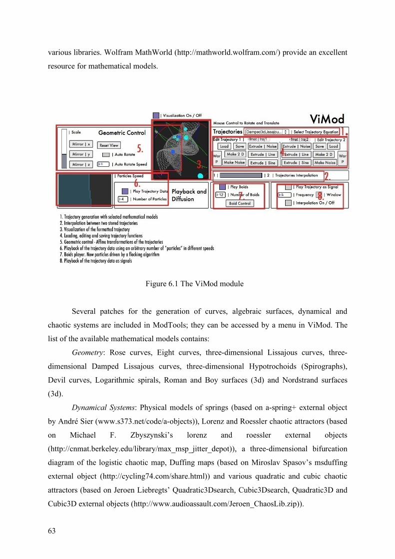
63

various libraries. Wolfram MathWorld (http://mathworld.wolfram.com/) provide an excellent

resource for mathematical models.

Figure 6.1 The ViMod module

Several patches for the generation of curves, algebraic surfaces, dynamical and

chaotic systems are included in ModTools; they can be accessed by a menu in ViMod. The

list of the available mathematical models contains:

Geometry: Rose curves, Eight curves, three-dimensional Lissajous curves, three-

dimensional Damped Lissajous curves, three-dimensional Hypotrochoids (Spirographs),

Devil curves, Logarithmic spirals, Roman and Boy surfaces (3d) and Nordstrand surfaces

(3d).

Dynamical Systems: Physical models of springs (based on a-spring+ external object

by André Sier (www.s373.net/code/a-objects)), Lorenz and Roessler chaotic attractors (based

on Michael F. Zbyszynski’s lorenz and roessler external objects

(http://cnmat.berkeley.edu/library/max_msp_jitter_depot)), a three-dimensional bifurcation

diagram of the logistic chaotic map, Duffing maps (based on Miroslav Spasov’s msduffing

external object (http://cycling74.com/share.html)) and various quadratic and cubic chaotic

attractors (based on Jeroen Liebregts’ Quadratic3Dsearch, Cubic3Dsearch, Quadratic3D and

Cubic3D external objects (http://www.audioassault.com/Jeroen_ChaosLib.zip)).

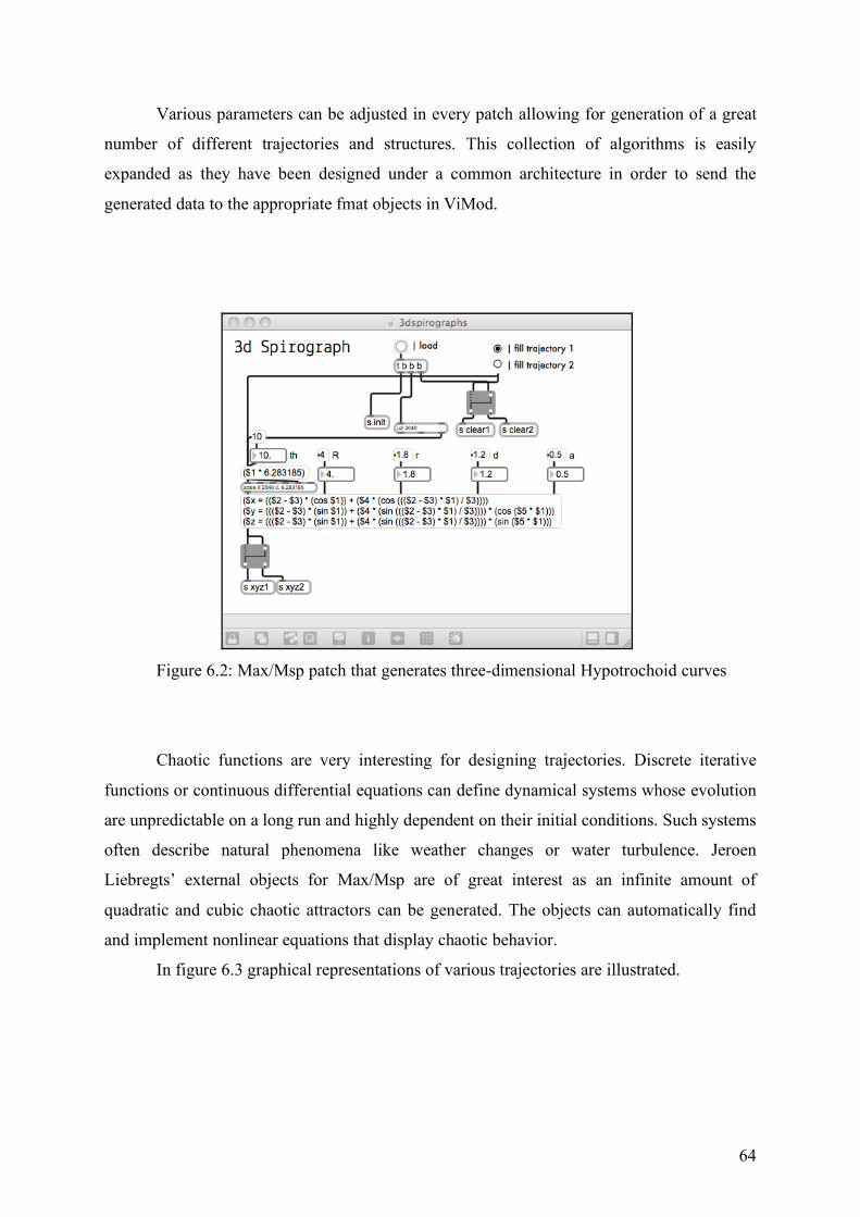
64

Various parameters can be adjusted in every patch allowing for generation of a great

number of different trajectories and structures. This collection of algorithms is easily

expanded as they have been designed under a common architecture in order to send the

generated data to the appropriate fmat objects in ViMod.

Figure 6.2: Max/Msp patch that generates three-dimensional Hypotrochoid curves

Chaotic functions are very interesting for designing trajectories. Discrete iterative

functions or continuous differential equations can define dynamical systems whose evolution

are unpredictable on a long run and highly dependent on their initial conditions. Such systems

often describe natural phenomena like weather changes or water turbulence. Jeroen

Liebregts’ external objects for Max/Msp are of great interest as an infinite amount of

quadratic and cubic chaotic attractors can be generated. The objects can automatically find

and implement nonlinear equations that display chaotic behavior.

In figure 6.3 graphical representations of various trajectories are illustrated.

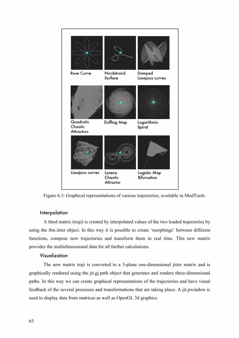
65

Figure 6.3: Graphical representations of various trajectories, available in ModTools.

Interpolation

A third matrix (traji) is created by interpolated values of the two loaded trajectories by

using the ftm.inter object. In this way it is possible to create ‘morphings’ between different

functions, compose new trajectories and transform them in real time. This new matrix

provides the multidimensional data for all further calculations.

Visualization

The new matrix traji is converted to a 3-plane one-dimensional jitter matrix and is

graphically rendered using the jit.gj.path object that generates and renders three-dimensional

paths. In this way we can create graphical representations of the trajectories and have visual

feedback of the several processes and transformations that are taking place. A jit.pwindow is

used to display data from matrices as well as OpenGL 3d graphics.

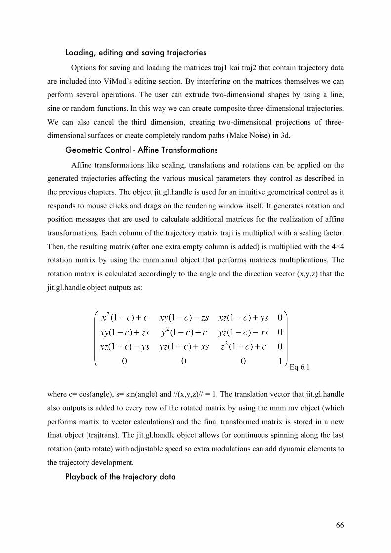
66

Loading, editing and saving trajectories

Options for saving and loading the matrices traj1 kai traj2 that contain trajectory data

are included into ViMod’s editing section. By interfering on the matrices themselves we can

perform several operations. The user can extrude two-dimensional shapes by using a line,

sine or random functions. In this way we can create composite three-dimensional trajectories.

We can also cancel the third dimension, creating two-dimensional projections of three-

dimensional surfaces or create completely random paths (Make Noise) in 3d.

Geometric Control - Affine Transformations

Affine transformations like scaling, translations and rotations can be applied on the

generated trajectories affecting the various musical parameters they control as described in

the previous chapters. The object jit.gl.handle is used for an intuitive geometrical control as it

responds to mouse clicks and drags on the rendering window itself. It generates rotation and

position messages that are used to calculate additional matrices for the realization of affine

transformations. Each column of the trajectory matrix traji is multiplied with a scaling factor.

Then, the resulting matrix (after one extra empty column is added) is multiplied with the 4×4

rotation matrix by using the mnm.xmul object that performs matrices multiplications. The

rotation matrix is calculated accordingly to the angle and the direction vector (x,y,z) that the

jit.gl.handle object outputs as:

Eq 6.1

where c= cos(angle), s= sin(angle) and //(x,y,z)// = 1. The translation vector that jit.gl.handle

also outputs is added to every row of the rotated matrix by using the mnm.mv object (which

performs martix to vector calculations) and the final transformed matrix is stored in a new

fmat object (trajtrans). The jit.gl.handle object allows for continuous spinning along the last

rotation (auto rotate) with adjustable speed so extra modulations can add dynamic elements to

the trajectory development.

Playback of the trajectory data

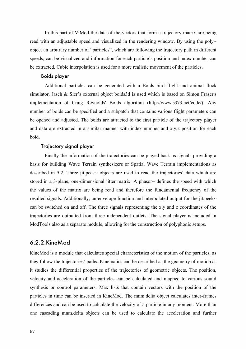
67

In this part of ViMod the data of the vectors that form a trajectory matrix are being

read with an adjustable speed and visualized in the rendering window. By using the poly~

object an arbitrary number of “particles”, which are following the trajectory path in different

speeds, can be visualized and information for each particle’s position and index number can

be extracted. Cubic interpolation is used for a more realistic movement of the particles.

Boids player

Additional particles can be generated with a Boids bird flight and animal flock

simulator. Jasch & Sier’s external object boids3d is used which is based on Simon Fraser's

implementation of Craig Reynolds' Boids algorithm (http://www.s373.net/code/). Any

number of boids can be specified and a subpatch that contains various flight parameters can

be opened and adjusted. The boids are attracted to the first particle of the trajectory player

and data are extracted in a similar manner with index number and x,y,z position for each

boid.

Trajectory signal player

Finally the information of the trajectories can be played back as signals providing a

basis for building Wave Terrain synthesizers or Spatial Wave Terrain implementations as

described in 5.2. Three jit.peek~ objects are used to read the trajectories’ data which are

stored in a 3-plane, one-dimensional jitter matrix. A phasor~ defines the speed with which

the values of the matrix are being read and therefore the fundamental frequency of the

resulted signals. Additionally, an envelope function and interpolated output for the jit.peek~

can be switched on and off. The three signals representing the x,y and z coordinates of the

trajectories are outputted from three independent outlets. The signal player is included in

ModTools also as a separate module, allowing for the construction of polyphonic setups.

6.2.2.KineMod

KineMod is a module that calculates special characteristics of the motion of the particles, as

they follow the trajectories’ paths. Kinematics can be described as the geometry of motion as

it studies the differential properties of the trajectories of geometric objects. The position,

velocity and acceleration of the particles can be calculated and mapped to various sound

synthesis or control parameters. Max lists that contain vectors with the position of the

particles in time can be inserted in KineMod. The mnm.delta object calculates inter-frames

differences and can be used to calculate the velocity of a particle in any moment. More than

one cascading mnm.delta objects can be used to calculate the acceleration and further

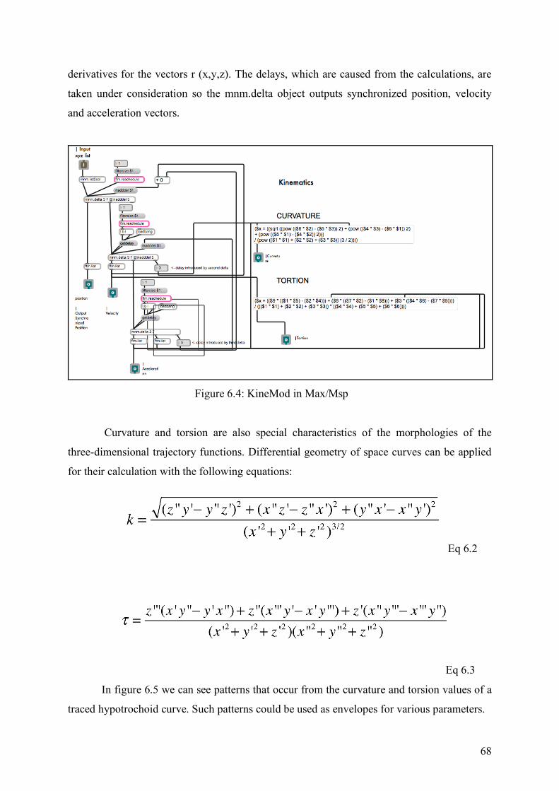
68

derivatives for the vectors r (x,y,z). The delays, which are caused from the calculations, are

taken under consideration so the mnm.delta object outputs synchronized position, velocity

and acceleration vectors.

Figure 6.4: KineMod in Max/Msp

Curvature and torsion are also special characteristics of the morphologies of the

three-dimensional trajectory functions. Differential geometry of space curves can be applied

for their calculation with the following equations:

Eq 6.2

Eq 6.3

In figure 6.5 we can see patterns that occur from the curvature and torsion values of a

traced hypotrochoid curve. Such patterns could be used as envelopes for various parameters.

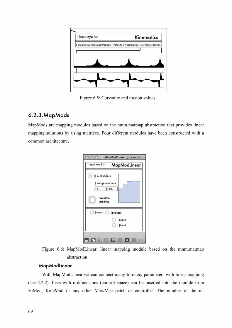
69

Figure 6.5: Curvature and torsion values

6.2.3.MapMods

MapMods are mapping modules based on the mnm.matmap abstraction that provides linear

mapping solutions by using matrices. Four different modules have been constructed with a

common architecture.

Figure 6.6: MapModLinear, linear mapping module based on the mnm.matmap

abstraction

MapModLinear

With MapModLinear we can connect many-to-many parameters with linear mapping

(see 4.2.2). Lists with n-dimensions (control space) can be inserted into the module from

ViMod, KineMod or any other Max/Msp patch or controller. The number of the m-

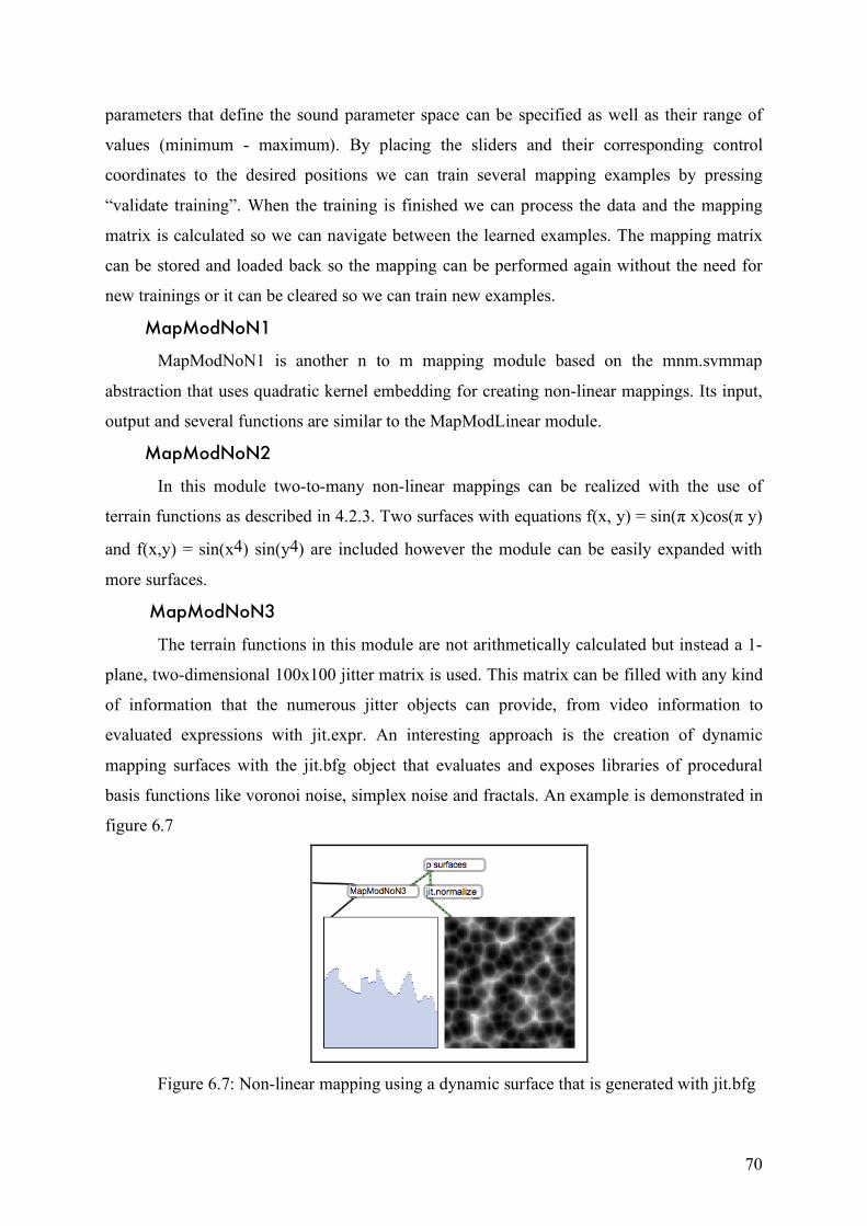
70

parameters that define the sound parameter space can be specified as well as their range of

values (minimum - maximum). By placing the sliders and their corresponding control

coordinates to the desired positions we can train several mapping examples by pressing

“validate training”. When the training is finished we can process the data and the mapping

matrix is calculated so we can navigate between the learned examples. The mapping matrix

can be stored and loaded back so the mapping can be performed again without the need for

new trainings or it can be cleared so we can train new examples.

MapModNoN1

MapModNoN1 is another n to m mapping module based on the mnm.svmmap

abstraction that uses quadratic kernel embedding for creating non-linear mappings. Its input,

output and several functions are similar to the MapModLinear module.

MapModNoN2

In this module two-to-many non-linear mappings can be realized with the use of

terrain functions as described in 4.2.3. Two surfaces with equations f(x, y) = sin(π x)cos(π y)

and f(x,y) = sin(x4) sin(y4) are included however the module can be easily expanded with

more surfaces.

MapModNoN3

The terrain functions in this module are not arithmetically calculated but instead a 1-

plane, two-dimensional 100x100 jitter matrix is used. This matrix can be filled with any kind

of information that the numerous jitter objects can provide, from video information to

evaluated expressions with jit.expr. An interesting approach is the creation of dynamic

mapping surfaces with the jit.bfg object that evaluates and exposes libraries of procedural

basis functions like voronoi noise, simplex noise and fractals. An example is demonstrated in

figure 6.7

Figure 6.7: Non-linear mapping using a dynamic surface that is generated with jit.bfg

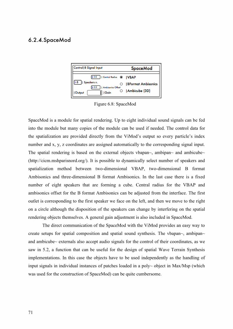
71

6.2.4.SpaceMod

Figure 6.8: SpaceMod

SpaceMod is a module for spatial rendering. Up to eight individual sound signals can be fed

into the module but many copies of the module can be used if needed. The control data for

the spatialization are provided directly from the ViMod’s output so every particle’s index

number and x, y, z coordinates are assigned automatically to the corresponding signal input.

The spatial rendering is based on the external objects vbapan~, ambipan~ and ambicube~

(http://cicm.mshparisnord.org/). It is possible to dynamically select number of speakers and

spatialization method between two-dimensional VBAP, two-dimensional B format

Ambisonics and three-dimensional B format Ambisonics. In the last case there is a fixed

number of eight speakers that are forming a cube. Central radius for the VBAP and

ambisonics offset for the B format Ambisonics can be adjusted from the interface. The first

outlet is corresponding to the first speaker we face on the left, and then we move to the right

on a circle although the disposition of the speakers can change by interfering on the spatial

rendering objects themselves. A general gain adjustment is also included in SpaceMod.

The direct communication of the SpaceMod with the ViMod provides an easy way to

create setups for spatial composition and spatial sound synthesis. The vbapan~, ambipan~

and ambicube~ externals also accept audio signals for the control of their coordinates, as we

saw in 5.2, a function that can be useful for the design of spatial Wave Terrain Synthesis

implementations. In this case the objects have to be used independently as the handling of

input signals in individual instances of patches loaded in a poly~ object in Max/Msp (which

was used for the construction of SpaceMod) can be quite cumbersome.

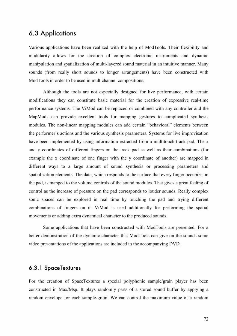
72

6.3 Applications

Various applications have been realized with the help of ModTools. Their flexibility and

modularity allows for the creation of complex electronic instruments and dynamic

manipulation and spatialization of multi-layered sound material in an intuitive manner. Many

sounds (from really short sounds to longer arrangements) have been constructed with

ModTools in order to be used in multichannel compositions.

Although the tools are not especially designed for live performance, with certain

modifications they can constitute basic material for the creation of expressive real-time

performance systems. The ViMod can be replaced or combined with any controller and the

MapMods can provide excellent tools for mapping gestures to complicated synthesis

modules. The non-linear mapping modules can add certain “behavioral” elements between

the performer’s actions and the various synthesis parameters. Systems for live improvisation

have been implemented by using information extracted from a multitouch track pad. The x

and y coordinates of different fingers on the track pad as well as their combinations (for

example the x coordinate of one finger with the y coordinate of another) are mapped in

different ways to a large amount of sound synthesis or processing parameters and

spatialization elements. The data, which responds to the surface that every finger occupies on

the pad, is mapped to the volume controls of the sound modules. That gives a great feeling of

control as the increase of pressure on the pad corresponds to louder sounds. Really complex

sonic spaces can be explored in real time by touching the pad and trying different

combinations of fingers on it. ViMod is used additionally for performing the spatial

movements or adding extra dynamical character to the produced sounds.

Some applications that have been constructed with ModTools are presented. For a

better demonstration of the dynamic character that ModTools can give on the sounds some

video presentations of the applications are included in the accompanying DVD.

6.3.1 SpaceTextures

For the creation of SpaceTextures a special polyphonic sample/grain player has been

constructed in Max/Msp. It plays randomly parts of a stored sound buffer by applying a

random envelope for each sample-grain. We can control the maximum value of a random

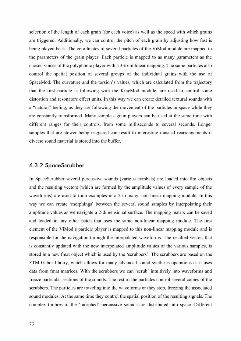
73

selection of the length of each grain (for each voice) as well as the speed with which grains

are triggered. Additionally, we can control the pitch of each grain by adjusting how fast is

being played back. The coordinates of several particles of the ViMod module are mapped to

the parameters of the grain player. Each particle is mapped to as many parameters as the

chosen voices of the polyphonic player with a 3-to-m linear mapping. The same particles also

control the spatial position of several groups of the individual grains with the use of

SpaceMod. The curvature and the torsion’s values, which are calculated from the trajectory

that the first particle is following with the KineMod module, are used to control some

distortion and resonators effect units. In this way we can create detailed textural sounds with

a “natural” feeling, as they are following the movement of the particles in space while they

are constantly transformed. Many sample - grain players can be used at the same time with

different ranges for their controls, from some milliseconds to several seconds. Longer

samples that are slower being triggered can result to interesting musical rearrangements if

diverse sound material is stored into the buffer.

6.3.2 SpaceScrubber

In SpaceScrubber several percussive sounds (various cymbals) are loaded into ftm objects

and the resulting vectors (which are formed by the amplitude values of every sample of the

waveforms) are used to train examples in a 2-to-many, non-linear mapping module. In this

way we can create ‘morphings’ between the several sound samples by interpolating their

amplitude values as we navigate a 2-dimensional surface. The mapping matrix can be saved

and loaded in any other patch that uses the same non-linear mapping module. The first

element of the ViMod’s particle player is mapped to this non-linear mapping module and is

responsible for the navigation through the interpolated waveforms. The resulted vector, that

is constantly updated with the new interpolated amplitude values of the various samples, is

stored in a new fmat object which is used by the ‘scrubbers’. The scrubbers are based on the

FTM Gabor library, which allows for many advanced sound synthesis operations as it uses

data from fmat matrices. With the scrubbers we can ‘scrub’ intuitively into waveforms and

freeze particular sections of the sounds. The rest of the particles control several copies of the

scrubbers. The particles are traveling into the waveforms or they stop, freezing the associated

sound modules. At the same time they control the spatial position of the resulting signals. The

complex timbres of the ‘morphed’ percussive sounds are distributed into space. Different

74

timbres occupy different positions in space when the particles are still while when there is

movement timbral transformations are synchronised with spatial movements. Complex sonic

patterns are shaped with impressive results.

75

Conclusions and further development A theoretical and practical exploration of how multidimensional data sets and their graphical

representations participate in the genesis of musical form has been made. Several ideas and

implementations were studied that dealt with both technology and artistic expression. A

union of them led to the term ‘composed instruments’ to describe the proposed

implementations. A set of tools was designed that allows for the construction of ‘naturally’

complex musical structures and patterns with a dynamic development in time and space.

Several algorithms for the generation of trajectories and surfaces, were examined and

realized, as they have been implemented for Wave Terrain Synthesis and other techniques.

More algorithms could be studied, which may give more interesting structures and

development in time. The solution that was proposed in ViMod, with the use of matrices for

storing the first 2048 values of the generated trajectories, is computationally efficient and

serves the initial idea of creating a host for a diverse collection of algorithms. However, this

solution has several limitations as it does not allow the dynamic control of the algorithms’

generative parameters neither their infinite physical development in time (when they are not

periodic). Similar limitations are present when the trajectories are read as signals. The

distinction between the control data rate and the signal rate processing is always a constrain

on applying algorithmic processes in various time scales. Naturally complex sounds are

achieved when their structuring algorithms are generated on a signal level (like Di Scipio’s

(2001) FIS synthesis method). A different architecture could be designed that takes advantage

of the continuous dynamic development of the algorithms in time. New systems could be

developed which can contain more algorithms for various physical particles’ interactions and

dynamic fields of applied forces. Feedback systems could also be introduced where the

information extracted from the trajectories could be mapped back to some of the generative

76

algorithm’s parameters.

The intuitive geometric control of the trajectories, the interpolations and the affine

transformations, especially the auto rotation function, partially solves this problem of the

periodicity of the trajectories as constant dynamic modulations and new patterns in space and

time are created.

The designed mapping modules provide great solutions for handling complex musical

systems with a large amount of parameters. Further development is also possible by

implementing new algorithms for non-linear mappings that represent dynamic behaviors.

Kernel methods or other statistical modeling techniques can be promising. Additionally, new

techniques can be developed for making the mapping system’s training realization easier.

Finally the unifying approach of using the trajectory functions for both sound

synthesis (or processing) and spatial rendering leads to very interesting results as complex

structures and sonic patterns unfold in time and space like in natural sounds. The case of

Spatial Wave Terrain Synthesis seems to be a promising field for further research. New three-

dimensional spatial rendering systems could be implemented that are controlled by signals. In

this way we could create three-dimensional spatial synthesizers to be used in compositions or

sound art installations.

77

References

Baalman M. A.J. (2010). Spatial Composition Techniques and Sound Spatialisation

Technologies. In Organized Sound, 15, 209-218

Berkhout, A. J., de Vries, D. and Vogel, P. (1993). Acousticcontrol by wave field synthesis.

Journal of the Acoustical Society of America, 93, 2764–2778.

Bevilacqua F., Muller R. & Schnell N. (2005). MnM: a Max/MSP mapping toolbox. In New

Interfaces for Musical Expression, Vancouver, 85-88

Blackwell, T., & Young, M. (2005). Live Algorithms. Retrieved February 15, 2011 from

www.timblackwell.com.

Boulanger, R. (2000). Scanned Synthesis &CSound @ CSounds.com, Retrieved March 12,

2012 from http://www.csounds.com/scanned

Bouman, O. (2005). Architecture, Liquid, Gas. Architectural Design, 75(1), Jan/Feb 2005,

14-22.

Bown, O., Eldridge, A. & McCormack, J. (2009). Understanding Interaction in

Contemporary Digital Music : From Instruments to Behavioural Objects. Organised

Sound 14(2), 188–196.

Braasch, J. (2005). A loudspeaker-based 3D sound projection using Virtual Microphone

Control (ViMiC). In 118th Convention of the Audio Engineering Society. Barcelona,

Spain.

Budon, O. (2000). Composing with Objects, Networks and Time Scales: An Interview with

Horacio Vaggione. Computer Music Journal 24(3), 9–22.

Cabaud, B. and Pottier, L. (2002). Le controle de la spatialisation multi-sources – Nouvelles

fonctionnalites dans Holophon version 2.2. Actes des Journees d’Informatique

Musicale, Marseille, France.

Chadabe, J. (2002). The limitations of mapping as a structural descriptive in electronic

instruments. Proc. of the 2002 Int. Conf. of New Interfaces for Musical Expression,

NIME02.

78

Choi, I. (1994) Interactive Exploration of a Chaotic Oscillator fot Generating Musical Signals

in Real-Time Concert Performance. Journal of the Franklin Institute, Special Issue:

Chaos and Nonlinear Dynamics.

Choi, I., Bargar, R. & Goudeseune, C. (1995). A Manifold Interface for a High Dimensional

Control Space. In Proceedings of the International Computer Music Conference. San

Francisco, California: International Computer Music Association, 181–184.

Christensen, E. (1996) The Musical Timespace. A Theory of Music Listening. Aalborg:

Aalborg University Press.

Cont, A., Coduys, T., Henry, C. (2004). Real-time Gesture Mapping in Pd Environment using

Neural Networks. In Proc.of the International Conference on New Interfaces for

Musical Expression 2004.

Di Scipio, A. (1999). Synthesis of environmental sound textures by iterated nonlinear

functions. Proceedings of the 2nd COST G-6 Workshop on Digital Audio Effects.

Trondheim: NTNU.

Di Scipio, A. (2001). Iterated nonlinear functions as a sound-generating engine. Leonardo,

34(3), 249–54.

Di Scipio, A. (2003). Sound is the Interface: From Interactive to Ecosystemic Signal

Processing. Organised Sound 8(3), 269–277.

Doornbusch, P. (2002). Composers’ views on mapping in algorithmic composition.

Organised Sound, 7(2), 145–156.

Filatriau, J. J., Arfib, D., & Couturier, J. M. (2006). Using visual textures for sonic textures

production and control. Proc. of the 9th Int. Conference on Digital Audio Effects

(DAFx-06), Montreal, Canada, 31-36.

Gold, R. (1979). A Terrain Reader. In C. P. Morgan (Ed.), The BYTE Book of Computer

Music. Byte Publications, Petersborough, NH.

Hunt, A. & Kirk, R. (2000). Mapping strategies for musical performance. In Wanderley and

Battier (eds.) Trends in Gestural Control of Music. Paris: IRCAM, Centre Pompidou.

Hunt, A., Wanderley, M. & Kirk, R. (2000). Towards a Model for Instrumental Mapping in

Expert Musical Interaction. In Proceedings of the 2000 International Computer Music

Conference. San Francisco, International Computer Music Association, 209 - 212.

James, S. G. (2005). Developing a flexible and expressive realtime polyphonic wave terrain

synthesis instrument based on a visual and multidimensional methodology. Master’s

thesis, Edith Cowan University, Perth, Australia.

79

Koenig, G.M. (1971). Summary: Observations on Compositional Theory. Utrecht: Institute of

Sonology

Koenig, G.M. (1985). Programmed Music. Retrieved April 18, 2012 from

http://www.koenigproject.nl/indexe.htm

Kwinter, S. (2002). Architectures of time, toward a theory of the event in modernist culture.

The MIT Press, London, England

Lossius T., Baltazar, P. & de la Hogue T. (2009): DBAP - Distance-Based Amplitude

Panning. In Proceedings of the International Computer Music Conference, Montreal,

17-21

Malham, D.G. & Myatt, A. (1995). 3-D Sound Spatialization using Ambisonic Techniques.

In Computer Music Journal, 19(4), 58-70.

McGee, R. & Wright, M. (2011). Sound Element Spatializer. In Proceedings of the

International Computer Music Conference. Huddersfield, England.

Mikelson, H. (2000a). Terrain Mapping Synthesis. In R. Boulanger (Ed.) The CSound Book:

perspectives in software synthesis, sound design, signal processing, and

programming. Cambridge, Massachusetts: MIT Press.

Mikelson, H. (2000b). Terrain Mapping with Dynamic Surfaces. The Csound Magazine.

Retrieved March 17, 2012 from http://www.csounds.com/ezine/spring2000/synthesis/

Mills, A. & De Souza, R. C. (1999). Gestural Sounds by Means of Wave Terrain Synthesis.

Congresso da Sociedade Brasileira de Computaçãoo XIX.

Mitsuhashi, Y. (1982). Audio Synthesis by Functions of Two Variables. Journal of the Audio

Engineering Society, 30(10), 701-706.

Momeni, A. & Wessel, D. (2003) Characterizing and controlling musical material intuitively

with geometric models In Proc. of the Conference on New Interfaces for Musical

Expression, Montreal, Canada.

Negrao, M. (2010). Strategies in Diffused Spatialization. Master’s thesis, Institute of

Sonology, The Hague.

Paine, G. (2002). Interactivity, Where to from Here? Organised Sound, 7(3), 295–304.

Peck, Robert W.(2003). Toward an interpretation of Xenakis's Nomos alpha. In Perspectives

of New Music, 2003

Place, T. & T. Lossius (2006): Jamoma: A modular standard for structuring patches in Max.

In Proceedings of the International Computer Music Conference 2006. New Orleans,

USA: International Computer Music Association.

80

Pulkki, V. (1997). Virtual sound source positioning using vector base amplitude panning. In

Journal of the Audio Engineering Society, 45(6), 456–466.

Ramakrishnan, C., Gomann, J. & Brummer L.(2006). The ZKM Klangdom. In Proc. of the

2006 conference on New Interfaces for Musical Expression, Paris, 140–143.

Rodet, X., Potard, Y. & Source, J-B. B. (1984). The CHANT Project: From the Synthesis of

the Singing Voice to Synthesis in General. Computer Music Journal, 8(3), 15-31

Salter, C. L., Baalman M. A.J., & Moody-Grigsby, D. (2007). Between Mapping,

Sonification and Composition: Responsive Audio Environments in Live Performance.

In International Computer Music Conference 2007, Copenhagen, Denmark, 27-31

August 2007.

Schumacher, M. & Bresson J. (2010). Spatial Sound Synthesis in Computer-Aided

Composition. In Organised Sound , 15(3), 271–289.

Sedes, A., Courribet B., and Thiebaut J. B. (2004). Visualization of Sound as a control

interface. In Proceedings of the Digital Audio Effects Conference, Naples.

Solomos, M. (2005). An introduction to Horacio Vaggione's musical and theoretical thought.

Contemporary Music Review, 24(4-5), 311-325

Spasov, M. (2011). Music Composition as an Act of Cognition: ENACTIV – interactive

multi-modal composing system. Organised Sound, 16(1), 69–86

Sterken, S. (2001). Towards a Space-Time Art: Iannis Xenakis’s Polytopes. Perspectives of

New Music, 39 (2), 262-273.

Sterken, S. (2007). Music as an Art of Space. Intersections between Music and Architecture

in the Work of Iannis Xenakis. In: Resonance. Essays on the Intersection of Music

and Architecture. Ames (USA): Culcidae Architectural Press.

Sterken, S. (2009). Immersive Strategies in Iannis Xenakis' Polytopes. Oase: Tijdschrift voor

Architectuur (78), 116-125.

Tenney, J. (1969). Computer Music Experiences, 1961-1964. Electronic Music Reports #1,

Utrecht: Institute of Sonology.

Thiebaut, J.-baptiste, Bello, J. P. & Schwarz, D. (2007). How Musical are Images? From

Sound Representation to Image Sonification: An Eco Systemic Approach. New York,

1, 183-187.

Torchia, R. H. and Lippe, C. (2004). Techniques for multichannel real-time spatial

distribution using frequencydomain processing. In Proceedings of the Conference on

New Interfaces for Musical Expression. Hamamatsu, Shizuoka, Japan, 116-119.

81

Truax, B. (1990). Composing with Real-time Granular Sound. Perspectives of New Music,

28(2), 120-134

Vaggione, H. (2001). Some Ontological Remarks about Music Composition Processes.

Computer Music Journal, 25(1), 54–61

Varèse, E. (1936). New York Times, Dec 6, 1936, section L, part N, p.7

Van Nort, D., Wanderley, M. M., Depalle, P. (2004) On the Choice of Mappings Based On

Geometric Properties, In Proc. of the International Conference on New Interfaces for

Musical Expression.

Van Nort, D.& Wanderley, M. (2006). Exploring the Effect of Mapping Trajectories on

Musical Performance. In Proc. 2006 Sound and Music Computing Conference (SMC),

19–24.

Van Nort, D.& Wanderley, M. (2007). Control strategies for navigation of complex sonic

spaces. In NIME '07 Proceedings of the 7th international conference on new

interfaces for musical expression, 379–382.

Wilson, Scott (2008). Spatial Swarm Granulation. In Proceedings of the International

Computer Music Conference. Belfast, Ireland.

Xenakis, I. (1985). Arts/Sciences: Alloys. New York: Pendragon Press.

Xenakis, I., Brown, R. & Source, J. R. (1987). Xenakis on Xenakis. Perspectives of New

Music, 25(1/2), 25th Anniversary Issue, 16-63.

Xenakis, I. (1992). Formalized music. (Rev. ed). New York: Pendragon Press.

Ξενάκης, I. (2001). Κείµενα περί Μουσικής και Αρχιτεκτονικής, Μάκης Σολωµός, επιµ. Τίνα

Πλυτά µτφ. Ψυχογιός, Αθήνα, 2001. – Xenakis, I. Essays on Music and Architecture.

Ed. Makis Solomos, Trans. Tina Plyta. Psichogios, Athens, 2001

82

Appendix

Contents of accompanying DVD

1. A pdf version of this document 2. ModTools for Max/Msp 3. Video demonstrations of SpaceTextures and SpaceGrubbers. (Multi-channel

sound is reduced to stereo) 4. A copy of my composition metaverse:

Title: metaverse Composer: Yiannis Tsirikoglou Date: 2011 Format: 4-channel tape provided in 4 mono files 44.100 Hz, 16 bits; 1st file goes to front left speaker, 2nd to front right, 3rd to rear right, and 4th to rear left. Duration: 13:50 min

‘metaverse is our collective online shared space, created by the convergence of virtually enhanced physical reality and physically persistent virtual space, including the sum of all virtual worlds, augmented reality and the internet. Coming from science fiction the term is also similar to multiverse, a term describing all the multiple possible universes (including the historical universe we consistently experience) that together comprise everything that exists: the entirety of space, time, matter, and energy as well as the physical laws and constants that determine them. Using some sinewaves and my sound card's input noise as raw material i try to create a complex "multiverse" of sound, following Xenakis suggestion for making something out of nothing. Like the creation of our universe. Algorithmically generated trajectories are controlling (using special mapping techniques) various quadrophonic digital synthesis processes in Max/Msp. As laws that lying under all sound processes, or as applied 'feld-forces', those algorithms exist in all possible time-scales, defning the sound objects in many ways, from their micro-structure transformations to their evolution in time and space. Geometry, chaos and probabilities are used to create strange, 'multidimensional' sound sculptures with altered physical characteristics. The form of the whole piece is like a turbulence, a dynamic process where sudden interruptions can occur, elements are defning main objects to become the background, they are disappearing to reappear transformed. The piece is moving between different energy states, tone and noise, movement and stasis.’