Multicomponent-Multiphase Equation of State for …prod.sandia.gov/techlib/access-control.cgi/2001/012619.pdf · Multicomponent-Multiphase Equation of State for Carbon ... or favoring

SANDIA REPORTSAND2001-2619Unlimited ReleasePrinted September 2001

Multicomponent-Multiphase Equation ofState for Carbon

Gerald I. Kerley and Lalit Chhabildas

Prepared bySandia National LaboratoriesAlbuquerque, New Mexico 87185 and Livermore, California 94550

Sandia is a multiprogram laboratory operated by Sandia Corporation,a Lockheed Martin Company, for the United States Department ofEnergy under Contract DE-AC04-94AL85000.

Approved for public release; further dissemination unlimited.

Issued by Sandia National Laboratories, operated for the United States Departmentof Energy by Sandia Corporation.

NOTICE: This report was prepared as an account of work sponsored by an agencyof the United States Government. Neither the United States Government, nor anyagency thereof, nor any of their employees, nor any of their contractors,subcontractors, or their employees, make any warranty, express or implied, orassume any legal liability or responsibility for the accuracy, completeness, orusefulness of any information, apparatus, product, or process disclosed, or representthat its use would not infringe privately owned rights. Reference herein to anyspecific commercial product, process, or service by trade name, trademark,manufacturer, or otherwise, does not necessarily constitute or imply its endorsement,recommendation, or favoring by the United States Government, any agency thereof,or any of their contractors or subcontractors. The views and opinions expressedherein do not necessarily state or reflect those of the United States Government, anyagency thereof, or any of their contractors.

Printed in the United States of America. This report has been reproduced directlyfrom the best available copy.

Available to DOE and DOE contractors fromU.S. Department of EnergyOffice of Scientific and Technical InformationP.O. Box 62Oak Ridge, TN 37831

Telephone: (865)576-8401Facsimile: (865)576-5728E-Mail: [email protected] ordering: http://www.doe.gov/bridge

Available to the public fromU.S. Department of CommerceNational Technical Information Service5285 Port Royal RdSpringfield, VA 22161

Telephone: (800)553-6847Facsimile: (703)605-6900E-Mail: [email protected] order: http://www.ntis.gov/ordering.htm

mailto:[email protected]

mailto:[email protected]

3

SAND2001-2619Unlimited Release

Printed September 2001

Abstract

The PANDA code is used to build a tabular equation of state (EOS) table for carbon. Themodel includes three solid phases (graphite, diamond, and metallic) and a fluid phase mix-ture containing three molecular components (C1, C2, and C3). Separate EOS tables werefirst constructed for each solid phase and for each molecular species in the fluid phase.Next, a mixture/chemical equilibrium model was used to construct a single multicompo-nent EOS table for the fluid phase from those for the individual chemical species. Finally,the phase diagram and multiphase EOS were determined from the Helmholtz free ener-gies. The model gives good agreement with experimental thermophysical data, static com-pression data, known phase boundaries, and shock-wave measurements. This EOS coversa wide range of densities (0 - 100 g/cm3) and temperatures (0 - 1.0×108K). The new EOStable can be accessed through the SNL-SESAME library as material number 7830.

Multicomponent-MultiphaseEquation of State for Carbon

Gerald I. Kerley, ConsultantKerley Technical Services

P.O. Box 709Appomattox, VA 24522-0709

Lalit C. ChhabildasShock Physics Applications Department

Sandia National Laboratories, P.O. Box 5800

Albuquerque, NM 87185-1181

Contents

Contents

Figures .................................................................................................................................5

Symbols and Units ...............................................................................................................6

1. Introduction....................................................................................................................7

1.1 Background..........................................................................................................7

1.2 Scope of Work .....................................................................................................8

2. EOS for Solid Phases.....................................................................................................9

2.1 General.................................................................................................................9

2.2 Graphite .............................................................................................................10

2.3 Diamond ............................................................................................................11

2.4 An Imperfect Form of Diamond........................................................................12

2.5 Metallic Solid ....................................................................................................13

3. EOS for Fluid Phase ....................................................................................................15

3.1 General...............................................................................................................15

3.2 Liquid Perturbation Theory ...............................................................................15

3.3 Monatomic Fluid Species (C1) ..........................................................................16

3.4 Polyatomic Fluid Species (Cn) ..........................................................................17

4. Thermal Electronic Contributions ...............................................................................21

4.1 General...............................................................................................................21

4.2 Basic Theory ......................................................................................................21

4.3 Charge Fluctuations ...........................................................................................22

4.4 Thermal Broadening ..........................................................................................23

4.5 Application to Carbon........................................................................................24

5. Results and Discussion ................................................................................................27

5.1 Multiphase EOS Calculations............................................................................27

5.2 Equilibrium Phase Diagram...............................................................................27

5.3 Melting Data ......................................................................................................29

5.4 Nonequilibrium Behavior ..................................................................................30

5.5 Shock-Wave Behavior .......................................................................................31

5.6 Shock Vaporization............................................................................................33

6. Conclusions and Recommendations ............................................................................35

References..........................................................................................................................37

Distribution ........................................................................................................................43

4 Carbon Equation of State

Figures

Figures

Figure 1. Compression curves for solid carbon phases...................................................10

Figure 2. Entropy vs. temperature for graphite and diamond. ........................................11

Figure 3. Density vs. temperature for graphite and diamond..........................................11

Figure 4. Thermal electronic contributions to entropy and pressure for metallic carbon. ................................................................................................25

Figure 5. Phase diagram for carbon. ...............................................................................28

Figure 6. Isobaric expansion data for carbon..................................................................29

Figure 7. Comparison of phase diagrams for carbon. .....................................................30

Figure 8. Shock-induced phase transitions in carbon. ....................................................31

Figure 9. Hugoniots for carbon at various initial densities. ............................................31

Figure 10. Hugoniot data for carbon aerogel foams .........................................................31

Figure 11. Sound speed for shock-compressed graphite...................................................32

Figure 12. Shock vaporization experiments on carbon. ....................................................33

Carbon Equation of State 5

Symbols and Units

Symbols and Units

ρ density [g/cm3]

V specific volume, [cm3/g]

T temperature [K]

P pressure [GPa]

E specific internal energy [MJ/kg]

A Helmholtz free energy [MJ/kg]

S entropy [MJ/(kg-K)]

β isothermal bulk modulus, [GPa]

EB cohesive energy of solid at zero pressure and temperature [MJ/kg]

ρ0 density of solid at zero pressure and temperature [g/cm3]

β0 bulk modulus of solid at zero pressure and temperature [GPa]

sound velocity [km/s]

shock velocity [km/s]

particle velocity [km/s]

R gas constant [8.31451×10-3 MJ/kg-mole-K]

W atomic or molecular weight [g/mole]

k Boltzmann’s constant [1.38066×10-29 MJ/K]

V 1 ρ⁄=

β ρ P∂ ρ∂⁄( )T=

CS

US

uP


Introduction

1. Introduction

1.1 Background

The unique properties of carbon have made it both a fascinating and an important subjectof experimental and theoretical studies for many years [1]-[4]. The contrast between itsbest-known elemental forms, graphite and diamond, is particularly striking. Graphite isblack, has a rather low density and high compressibility (close to that of magnesium), andis greasy enough to be useful as a lubricant and in pencil leads. Diamond is brilliantlytranslucent, 60% more dense than graphite, less compressible than either tungsten or co-rundum, and its hardness makes it useful for polishing and cutting. This variability inproperties, as well as that observed among the many classes of carbon compounds, arisesbecause of profound differences in electronic structure of the carbon bonds [5].

A number of other solid forms of carbon are known. Pyrolytic graphite [6] is a polycrys-talline material in which the individual crystallites have a structure quite similar to that ofnatural graphite. Fullerite (solid C60), discovered only ten years ago [7], consists of giantmolecules in which the atoms are arranged into pentagons and hexagons on the surface ofa spherical cage. Amorphous carbon [8][9], including carbon black and ordinary soot, is adisordered form of graphite in which the hexagonally bonded layers are randomly orient-ed. Glassy carbons [9][10], on the other hand, have more random structures. Many otherstructures have been discussed [1][9].

Because of its high melting point, low thermal expansion, and high heat capacity, graphiteis often used in structural materials and composites, as in heat shields for space reentry ve-hicles. In addition to its importance as a pure material, there has been considerable interestin carbon because of its formation in the detonation products of explosives and in the de-composition products of hydrocarbons, plastics, and other compounds [11]-[13].

The carbon phase diagram exhibits some interesting features, some of which are still notcompletely understood. In the numerical simulation of dynamic phenomena, it is impor-tant to account for the phase transition from graphite to diamond. However, this transitiondoes not occur at the equilibrium pressure in shock-wave experiments. While a full non-equilibrium model of this transition is not yet available, we have shown that many aspectsof the behavior can be reproduced by treating diamond as an imperfect crystal [11][12].

The high melting point has limited experimental investigations of the liquid phase, butsome information has been obtained using dynamic methods. A recent discussion of themethods and their difficulties is given by Musella, et al. [14]. The graphite-liquidboundary is known to exhibit a temperature maximum at about 5-6 GPa [15]. This featureshows that liquid carbon is less dense than graphite at low pressure but becomes denser asthe pressure is increased, indicating a rather significant change in compressibility. Theconductivity of liquid carbon also depends upon pressure—insulating behavior is ob-served at low pressures, metallic behavior at higher pressures.


Introduction

Carbon does not vaporize at atmospheric pressure; it sublimes at a temperature below thegraphite-liquid-vapor triple point [14]. Analysis of the sublimation data shows that poly-atomic molecules are present in the vapor [16][17].

1.2 Scope of Work

In this work, we use the PANDA code [18] to construct a multicomponent-multiphaseEOS model for carbon that is valid over a wide range of densities and temperatures. Theresults are put into tabular form for use in numerical simulations using the Sandia hydro-code CTH and other codes utilizing the SESAME format [19]-[23].

The model includes three solid phases—graphite, diamond, and metallic solid. Two mod-els are created for diamond—the perfect crystal, used to compute the equilibrium proper-ties, and an imperfect form, used to describe nonequilibrium behavior. The solid modelsare discussed in Section 2.

Our model for the fluid phase (liquid, vapor, and supercritical regions) allows for the ex-istence of several chemical species—the monatomic form C1, which is metallic, and thepolyatomic molecules C2, C3, C4, and C5. The PANDA mixture-chemical equilibriummodel is used to construct a single EOS for the fluid phase. C 3 molecules are shown to beimportant, not only in the vapor phase, but also in the liquid phase at low pressures. Thetransition from C3 to C1 under pressure is found to explain the distinctive character of thegraphite-melting curve. The liquid models are discussed in Section 3.

The models for the metallic solid and liquid also include contributions from thermal elec-tronic excitation and ionization, which become very important at high temperatures. Thesecontributions were calculated using the PANDA ionization equilibrium model. The ver-sion used here, which contains some new features that were not discussed in the originalPANDA manual, is described in Section 4.

Results of the model are discussed in Section 5. Good agreement is obtained with a varietyof experimental information—the phase diagram, shock-wave data, including shock-induced phase transitions, isobaric expansion, sound speed in the shocked state, andshock-vaporization experiments.

Conclusions and recommendations are given in Section 6.


EOS for Solid Phases

2. EOS for Solid Phases

2.1 General

We will consider three solid phases of carbon in this work—graphite, diamond, and metal-lic. We will also consider an imperfect form of diamond, used in treating deviations fromthe equilibrium phase diagram. The thermodynamic functions for the solid phases are ex-pressed as sums of four terms that are assumed to be separable and additive:

, (1)

, (2)

. (3)

The subscripts and denote contributions from the zero-Kelvin curve and lattice vibra-tions, respectively. The subscript denotes the contributions from thermal electronic ex-citations, which were included only for the metallic phase; this term is discussed inSection 2.3. In order to give a consistent energy zero for all three phases, the constants

were chosen according to

, (4)

where is the density of the phase at 298K and ambient pressure, and is itsenthalpy of formation relative to graphite.

The zero-Kelvin curves were fit to the Birch-Murnaghan equation [24],

, (5)

, (6)

where , and , , and are constants. To insure correct asymptotic be-havior at high densities, the PANDA extrapolation formula [18], which is based on Tho-mas-Fermi-Dirac (TFD) theory, was used at high pressures.

The lattice-vibrational terms were computed using the well-known Debye and Einsteinmodels. The equations for these models are given in the PANDA manual [18], and we willlimit the present discussion to points specific to carbon.

P ρ T,( ) Pc ρ( ) Pl ρ T,( ) Pe ρ T,( )+ +=

E ρ T,( ) Ec ρ( ) El ρ T,( ) Ee ρ T,( ) ∆Eb–+ +=

A ρ T,( ) Ec ρ( ) Al ρ T,( ) Ae ρ T,( ) ∆Eb–+ +=

c le

∆Eb

∆Eb Ec ρ298( ) Al ρ298 298,( ) Ae ρ298 298,( )+ +[ ] ∆ Hfo

298( )–=

ρ298 ∆Hfo

298( )

Pc ρ( ) 32---β0 η7 3/ η5 3/–( ) 1 3

4--- η2 3/ 1–( ) β′0 4–( )+=

Ec ρ( )9β0

8ρ0--------- η2 3⁄

1–( )2 1

2--- η2 3/ 1–( ) β′0 4–( ) 1+=

η ρ ρ0⁄= ρ0 β0 β′0



2.2 Graphite

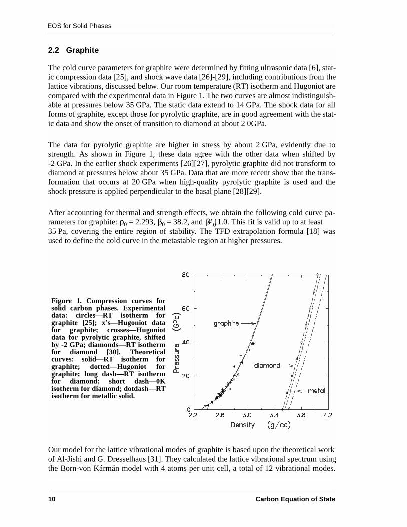
The cold curve parameters for graphite were determined by fitting ultrasonic data [6], stat-ic compression data [25], and shock wave data [26]-[29], including contributions from thelattice vibrations, discussed below. Our room temperature (RT) isotherm and Hugoniot arecompared with the experimental data in Figure 1. The two curves are almost indistinguish-able at pressures below 35 GPa. The static data extend to 14 GPa. The shock data for allforms of graphite, except those for pyrolytic graphite, are in good agreement with the stat-ic data and show the onset of transition to diamond at about 2 0GPa.

The data for pyrolytic graphite are higher in stress by about 2 GPa, evidently due tostrength. As shown in Figure 1, these data agree with the other data when shifted by-2 GPa. In the earlier shock experiments [26][27], pyrolytic graphite did not transform todiamond at pressures below about 35 GPa. Data that are more recent show that the trans-formation that occurs at 20 GPa when high-quality pyrolytic graphite is used and theshock pressure is applied perpendicular to the basal plane [28][29].

After accounting for thermal and strength effects, we obtain the following cold curve pa-rameters for graphite: ρ0 = 2.293, β0 = 38.2, and = 11.0. This fit is valid up to at least35 Pa, covering the entire region of stability. The TFD extrapolation formula [18] wasused to define the cold curve in the metastable region at higher pressures.

Our model for the lattice vibrational modes of graphite is based upon the theoretical workof Al-Jishi and G. Dresselhaus [31]. They calculated the lattice vibrational spectrum usingthe Born-von Kármán model with 4 atoms per unit cell, a total of 12 vibrational modes.

β′0

Figure 1. Compression curves forsolid carbon phases. Experimentaldata: circles—RT isotherm forgraphite [25]; x’s—Hugoniot datafor graphite; crosses—Hugoniotdata for pyrolytic graphite, shiftedby -2 GPa; diamonds—RT isothermfor diamond [30]. Theoreticalcurves: solid—RT isotherm forgraphite; dotted—Hugoniot forgraphite; long dash—RT isothermfor diamond; short dash—0Kisotherm for diamond; dotdash—RTisotherm for metallic solid.



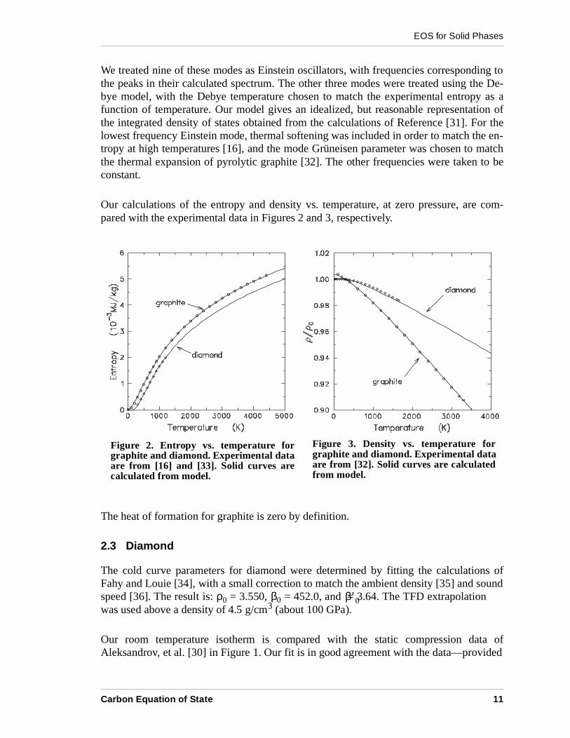
We treated nine of these modes as Einstein oscillators, with frequencies corresponding tothe peaks in their calculated spectrum. The other three modes were treated using the De-bye model, with the Debye temperature chosen to match the experimental entropy as afunction of temperature. Our model gives an idealized, but reasonable representation ofthe integrated density of states obtained from the calculations of Reference [31]. For thelowest frequency Einstein mode, thermal softening was included in order to match the en-tropy at high temperatures [16], and the mode Grüneisen parameter was chosen to matchthe thermal expansion of pyrolytic graphite [32]. The other frequencies were taken to beconstant.

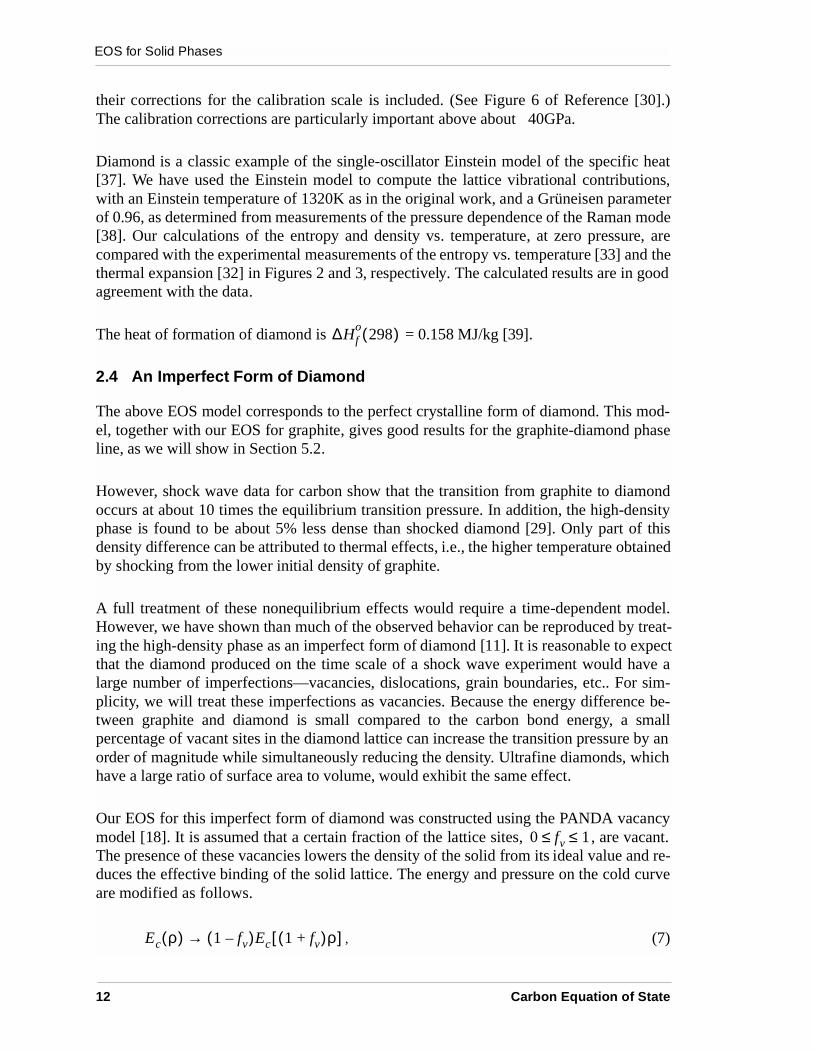
Our calculations of the entropy and density vs. temperature, at zero pressure, are com-pared with the experimental data in Figures 2 and 3, respectively.

The heat of formation for graphite is zero by definition.

2.3 Diamond

The cold curve parameters for diamond were determined by fitting the calculations ofFahy and Louie [34], with a small correction to match the ambient density [35] and soundspeed [36]. The result is: ρ0 = 3.550, β0 = 452.0, and = 3.64. The TFD extrapolationwas used above a density of 4.5 g/cm3 (about 100 GPa).

Our room temperature isotherm is compared with the static compression data ofAleksandrov, et al. [30] in Figure 1. Our fit is in good agreement with the data—provided

Figure 2. Entropy vs. temperature forgraphite and diamond. Experimental dataare from [16] and [33]. Solid curves arecalculated from model.

Figure 3. Density vs. temperature forgraphite and diamond. Experimental dataare from [32]. Solid curves are calculatedfrom model.

β′0



their corrections for the calibration scale is included. (See Figure 6 of Reference [30].)The calibration corrections are particularly important above about 40GPa.

Diamond is a classic example of the single-oscillator Einstein model of the specific heat[37]. We have used the Einstein model to compute the lattice vibrational contributions,with an Einstein temperature of 1320K as in the original work, and a Grüneisen parameterof 0.96, as determined from measurements of the pressure dependence of the Raman mode[38]. Our calculations of the entropy and density vs. temperature, at zero pressure, arecompared with the experimental measurements of the entropy vs. temperature [33] and thethermal expansion [32] in Figures 2 and 3, respectively. The calculated results are in goodagreement with the data.

The heat of formation of diamond is = 0.158 MJ/kg [39].

2.4 An Imperfect Form of Diamond

The above EOS model corresponds to the perfect crystalline form of diamond. This mod-el, together with our EOS for graphite, gives good results for the graphite-diamond phaseline, as we will show in Section 5.2.

However, shock wave data for carbon show that the transition from graphite to diamondoccurs at about 10 times the equilibrium transition pressure. In addition, the high-densityphase is found to be about 5% less dense than shocked diamond [29]. Only part of thisdensity difference can be attributed to thermal effects, i.e., the higher temperature obtainedby shocking from the lower initial density of graphite.

A full treatment of these nonequilibrium effects would require a time-dependent model.However, we have shown than much of the observed behavior can be reproduced by treat-ing the high-density phase as an imperfect form of diamond [11]. It is reasonable to expectthat the diamond produced on the time scale of a shock wave experiment would have alarge number of imperfections—vacancies, dislocations, grain boundaries, etc.. For sim-plicity, we will treat these imperfections as vacancies. Because the energy difference be-tween graphite and diamond is small compared to the carbon bond energy, a smallpercentage of vacant sites in the diamond lattice can increase the transition pressure by anorder of magnitude while simultaneously reducing the density. Ultrafine diamonds, whichhave a large ratio of surface area to volume, would exhibit the same effect.

Our EOS for this imperfect form of diamond was constructed using the PANDA vacancymodel [18]. It is assumed that a certain fraction of the lattice sites, , are vacant.The presence of these vacancies lowers the density of the solid from its ideal value and re-duces the effective binding of the solid lattice. The energy and pressure on the cold curveare modified as follows.

, (7)

∆Hfo

298( )

0 fv 1≤ ≤

Ec ρ( ) 1 fv–( )Ec 1 fv+( )ρ[ ]→



. (8)

The vacancies also make a contribution to the entropy, which is computed by assuming thevacant sites to be randomly distributed. The result is

, (9)

where R is the gas constant and W is the atomic weight.

In the present work, we find that assuming only 3% of the sites to be vacant ( )gives satisfactory agreement with the shock data.

2.5 Metallic Solid

Simple theoretical arguments, together with analogy to the other Group IVA elements (Si,Ge, Sn, and Pb), indicate that carbon should transform to a metallic phase at sufficientlyhigh pressures. However, the transition pressure and structure of this phase have not beenestablished experimentally. There could even be more than one high-pressurephase transition.

Theoretical calculations have been made for many different structures [34][40]-[43]. Ofall that have been considered, the fourfold coordinated structure bc-8 (or Si-III) is by farthe most stable energetically [34]. The sixfold coordinated structures (sc and β-Sn) arehigher in energy and also kinetically unstable. The most highly coordinated structures(fcc, bcc, hcp) are highest in energy.

We assume that the metallic phase is bc-8 in this work. The cold curve parameters weredetermined by fitting the calculations of Fahy and Louie [34]. The result is: ρ0 = 3.656, β0= 440, and = 3.7. (Our value of β0 differs slightly from that given by Fahy and Louie,who used a different formula to fit the EOS in the region near zero pressure.) The TFD ex-trapolation was used above a density of 4.5 g/cm3 (about 100 GPa). Our room temperatureisotherm for the metallic phase is shown in Figure 1.

The lattice vibrational contributions for the bc-8 phase were calculated using the Debyemodel. In the absence of experimental data, the Debye temperature Θ was estimated fromthe sound speed, using the Slater formula with a Poisson’s ratio of 1/3 (Equation 2.1 ofReference [18]); the result was Θ = 1270K. The Grüneisen parameter Γ was estimatedfrom the cold curve, using the Dugdale-MacDonald formula (Equation 4.19 of Reference[18]); the result was Γ = 1.35.

The electronic terms in Equations. (1)-(3) were computed from the ionization equilibriummodel discussed in Section 4.

Pc ρ( ) 1 fv–( )Pc 1 fv+( )ρ[ ] 1 fv+( )⁄→

∆Svac R fv fvln 1 fv–( ) 1 fv–( )ln+⁄[ ] W⁄–=

fv 0.03=

β′0



Fahy and Louie also predicted that the energy of the bc-8 phase is higher than that of dia-mond by 5.5 MJ/kg. After correcting for thermal and zero-point energy terms, we obtain aheat of formation of 5.3 MJ/kg for the bc-8 phase.

As we will show in Section 3.3, the bct-8 cold curve is also used in our model for themonatomic liquid phase. Equations (5) and (6) only define the cold curve in the compres-sion region. The LJ MATCH option in PANDA was used to define the tension region,which is needed for the liquid model. In order to insure the correct value of the binding en-ergy as the density approaches zero, the energy on the cold curve is representedby [18]

for . (10)

This option requires three parameters— , , and . ( , , and are determinedby requiring that the energy, pressure, and first derivative of the pressure are continuous atthe match density.)

The binding energy was determined from the heat of formation for the bct-8 phase and thatfor carbon gas [39], along with thermal and zero-point energy corrections. The result was

= 55.0 MJ/kg. Values for the other two parameters, which are less critical, were ob-tained from those we previously obtained for iron [44], by scaling according to density:

= 3.25, = 0.75.

∆Hfo

298( )

EB

Ec ρ( ) f1ρf2 f3ρ

fLJ– EB+= ρ ρLJ≤

EB ρLJ fLJ f1 f2 f3

EB

ρLJ fLJ


EOS for Fluid Phase

3. EOS for Fluid Phase

3.1 General

Our EOS for the fluid phase—which includes the liquid, gas, and supercritical regions—allows for the existence of several molecular species (Cn, n=1,2,3,...). The EOS for eachspecies is calculated using the PANDA liquid model [18]. The Helmholtz free energy hasthe form

. (11)

Here includes the contributions from the intermolecular forces and the thermal mo-tions of the molecular centers of mass. is the contribution from internal rotational andvibrational degrees of freedom, included only for the polyatomic species. is the contri-bution from thermal electronic excitations, included only for the monatomic and diatomicspecies. The constants were chosen to give the same energy zero as for the solidphases. The other thermodynamic quantities were computed from the usualthermodynamic relations.

After separate EOS tables have been constructed for each chemical species, the PANDAmixture model is used to construct an EOS for the complete system. This model employsthe ideal mixing approximation—the mixture components have equal temperatures andpressures, their volumes are additive, and the entropy of mixing is that for complete ran-domness. The chemical composition is computed from the principle of chemical equilibri-um, i.e., by minimizing the free energy. Hence, the molecular composition varies withdensity and temperature.

3.2 Liquid Perturbation Theory

The first term in Eq. (11), , was calculated using a version of liquid perturbation theorycalled the CRIS model [45][46]. This model has been discussed in detail in previous work,and we will review only a few points here.

The thermodynamic properties of a fluid are determined by the potential energy φ of amolecule in the field of neighboring molecules. The free energy can be written interms of this function by using a perturbation expansion about the properties of an ideal-ized hard-sphere fluid,

, (12)

where N0 is Avogadro’s number and W is the molecular weight. Here is the free energyfor a fluid of hard spheres with diameter σ, and , the first-order correction, is an aver-age of φ over all configurations of the hard sphere fluid. In the CRIS model, the

A ρ T,( ) Aφ ρ T,( ) Avr ρ T,( ) Ae ρ T,( ) ∆Eb–+ +=

AφAvr

Ae

∆Eb

Aφ

Aφ

Aφ ρ T,( ) A0 ρ T σ, ,( ) N0 W⁄( ) φ⟨ ⟩ 0 ∆A+ +=

A0φ⟨ ⟩ 0


EOS for Fluid Phase

hard-sphere diameter σ is defined by a variational principle that minimizes , where includes all corrections to the first two terms. This approach defines the hard-sphere

system having a structure that is closest to that of the real fluid. The corrections are thencomputed from approximate expressions.

The function φ depends upon the intermolecular forces and is related to the zero-Kelvinenergy of the solid phase by

, (13)

where xs denotes the configuration of the neighbors in the solid at density ρ. To calculatethe fluid properties from Eq. (12), φ must be averaged over many configurations of neigh-bors that are different from those of the solid. Since current theories of the electronicstructure of matter are not sufficiently accurate for calculating φ, except for very simplesystems, the CRIS model idealizes the fluid configurations and approximates φ by

(14)

Here ρ is the actual density of the fluid, and ρs is the solid density having the same nearestneighbor distance as that of the given fluid configuration. For this approximation to bevalid, the short-range structure of the solid must be reasonably close to that in the liquid.When several solid structures are possible, one must choose the one that gives the best re-sults for the liquid or adjust the cold curve to fit the data.

3.3 Monatomic Fluid Species (C1)

Since theoretical calculations show that the properties of solid carbon vary markedly withstructure, there is ambiguity as to which cold curve to use in the model for monatomicfluid carbon. However, the fact that liquid carbon exhibits metallic conductivity at pres-sures above ~5 GPa [4] suggests that the cold curve for a metallic solid structure should beused. Of all the structures that have been studied theoretically, only bc-8 has a binding en-ergy of the right magnitude to reproduce the observed melting point when used with thefluid model. In this work, therefore, we have used the same function for the C 1 fluid asfor the bc-8 phase, discussed in Section 2.5. As a result, the energy shift is also thesame as for the bc-8 phase.

As in previous work on liquid metals, the EFAC energy parameter in the CRIS model wasused to “fine tune” the results. We set EFAC = 1.45 MJ/kg (2.6% of the cohesive energy)to match the graphite melting line at high pressures (Section 5.2). As noted in Section 2.5,two parameters in the PANDA LJ MATCH option, which defines the behavior of the zero-Kelvin isotherm in tension, were estimated from those for iron [44].

∆A∆A

Ec ρ( ) N0 W⁄( )φ xs( )=

φ ρ ρs⁄( )Ec ρs( )≈

Ec

Ec∆Eb


EOS for Fluid Phase

The thermal electronic term for the C1 fluid, which is the same as that for the bc-8 solid, isdiscussed in Section 4. for monatomic carbon, since it has no internal degrees offreedom.

3.4 Polyatomic Fluid Species (Cn)

Calculations using our EOS for the C1 fluid, together with the graphite and diamond EOS,give good agreement with experimental data at high pressures. In particular, it reproducesthe negative slope of the graphite melting curve above 6 GPa and the shock data that lie inthe liquid region (Section 5.2). At low pressures, the positive slope of the graphite meltingcurve shows that the liquid is less dense than graphite, which is inconsistent with our mod-el for the C1 fluid. The conductivity of the liquid also decreases at low pressures [4][14].These observations indicate a significant change in the liquid structure at low pressures.Good agreement with the low-pressure data can be obtained when polyatomic moleculesare allowed to form in the liquid.

In calculating thermodynamic properties for the polyatomic species, Eq. (11), the C n mol-ecules were treated as freely rotating, and hence spherically symmetric, in computing thecontributions from center-of-mass motion, . Contributions from the internal rotationsand vibrations, , were computed using the rigid rotator-harmonic oscillator approxima-tion [18], with parameters taken from the JANAF Tables [16]. For C2, the thermal elec-tronic term was also calculated from the energy and degeneracy of the lowest-lyingexcited state [16][18]. The energy shifts were determined from the gas-phase heats offormation [16]. Since all of these parameters can be fixed rather easily, the only challengeis to determine the cold curves needed by the liquid model, for computing .

There are no direct experimental measurements of the cold curves or intermolecular forcesfor Cn molecules, and first-principles quantum-mechanical calculations are beyond thescope of this report—probably beyond the present state of the art. Therefore, we will haveto estimate the cold curves using simple, semi-empirical arguments. As we will show,these arguments demonstrate that C3 is the only important polyatomic species in the liquidphase.

Given the lack of information, it is desirable to minimize the number of parameters used inthe model as much as possible. With this end in mind, the cold curves were represented us-ing the so-called “universal” formula of Rose, et al. [47]. In PANDA, this expression iswritten in the form [18]

, (15)

, (16)

where

Avr 0=

AφAvr

Ae∆Eb

Aφ

Ec ρs( ) EB EB 1 a 0.05a3

+ +( )exp a–( )–=

Pc ρs( ) β0EB ρ0⁄ ρ0 ρs⁄( )1 3/ ρs a 0.15a2– 0.05a3

+( )exp a–( )–=


EOS for Fluid Phase

. (17)

Here , , and are the cohesive energy, density, and bulk modulus of the condensedphase at zero pressure. These parameters were further restricted by requiring that, for giv-en values of and , be chosen to make Eq. (16) extrapolate smoothly into theTFD curve at high pressures. This additional constraint defines a family of cold curves forthe various Cn species, determined only by the two parameters and .

In order to estimate values for the parameters and , we consider next the electronicstructure of a Cn molecule, which has been studied by Pitzer and Clementi [17]. Theyshowed that a conventional chemical valence picture of the bonding is

The molecules are linear, the carbon atoms are doubly bonded (one σ- and one π-bond),and each of the terminal carbon atoms has an unbonded electron pair. In further support ofthis picture, we note that the average bond energies, calculated from the heats of formation[16], are as follows: C2 - 594 kJ, C3 - 661 kJ, C4 - 624 kJ, C5 - 640 kJ. These values are ingood agreement with the typical C-C double bond energy (615 kJ, compared with 347 fora single bond and 812 for a triple bond [5]).

For purposes of comparison, N2, O2, and CO2 have the following structures:

The intermolecular forces in these three compounds are due primarily to interactions be-tween the terminal electrons and the π-electron groups with those on neighboring mole-cules. We have previously obtained values of in the range 0.3-0.4 MJ/kg for thesecompounds. Sensitivity studies demonstrate that such values are much too small to allowformation of Cn molecules in the liquid state.

However, the electronic structure of a Cn molecule differs from that of N2, O2, and CO2 ina very important way—the terminal carbon atoms in Cn are deficient in electrons. Eachterminal carbon is capable of forming two additional covalent bonds, as in the interior ofthe chain, or interacting with surrounding molecules by metallic bonding (delocalizedelectrons). There should be an especially large contribution to the interaction energy fromneighboring molecules aligned along the same axis.

Define to be the average energy of interaction of a Cn molecule with its neighbors.Each atom in the chain will have an energy in the four directions perpendicular to theaxis. Each terminal atom will also have an energy in the parallel direction. Hence

a 3 β0 ρ0EB⁄ ρ0 ρs⁄( )1 3/ 1–[ ]=

EB ρ0 β0

EB ρ0 β0

EB ρ0

EB ρ0

� ��

��

EB

εnεp

εt


EOS for Fluid Phase

, (18)

where the factor of 1/2 is needed because the interaction energy is shared between themolecule and its neighbors and must not be counted twice.

The terminal interaction term should be a significant fraction of the C-C double bond en-ergy. Therefore, we will write , where is an adjustable parameter. If themolecules are freely rotating, the probability is 1/3 that a neighboring molecule will havethe correct orientation to form a bond with a terminal atom. Hence a “nominal” value of would be 0.33. As we will show below, the value 0.40 gives good agreement with themelting temperature. The other interaction term, , should be roughly equal to the energyof interaction between planes in graphite, ~4.2 kJ [48], much smaller than the value of .Using these estimates, together with Equation (18), the binding energy for a Cnmolecule is

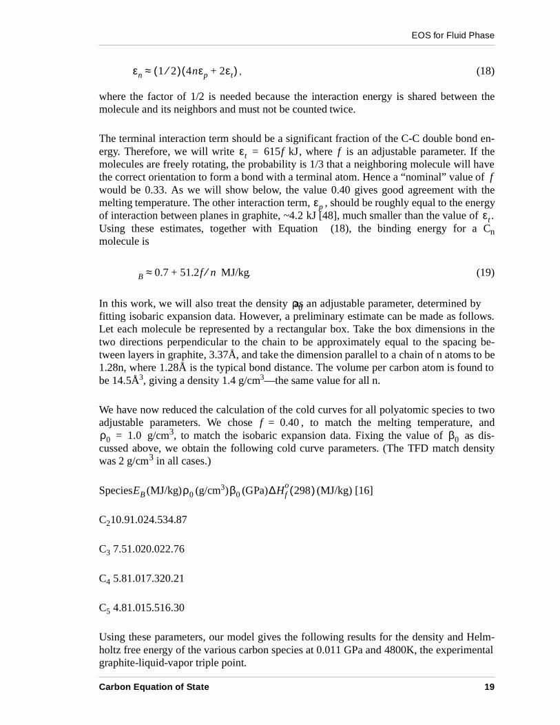
. (19)

In this work, we will also treat the density as an adjustable parameter, determined byfitting isobaric expansion data. However, a preliminary estimate can be made as follows.Let each molecule be represented by a rectangular box. Take the box dimensions in thetwo directions perpendicular to the chain to be approximately equal to the spacing be-tween layers in graphite, 3.37Å, and take the dimension parallel to a chain of n atoms to be1.28n, where 1.28Å is the typical bond distance. The volume per carbon atom is found tobe 14.5Å3, giving a density 1.4 g/cm3—the same value for all n.

We have now reduced the calculation of the cold curves for all polyatomic species to twoadjustable parameters. We chose , to match the melting temperature, and

g/cm3, to match the isobaric expansion data. Fixing the value of as dis-cussed above, we obtain the following cold curve parameters. (The TFD match densitywas 2 g/cm3 in all cases.)

Species (MJ/kg) (g/cm3) (GPa) (MJ/kg) [16]

C210.91.024.534.87

C3 7.51.020.022.76

C4 5.81.017.320.21

C5 4.81.015.516.30

Using these parameters, our model gives the following results for the density and Helm-holtz free energy of the various carbon species at 0.011 GPa and 4800K, the experimentalgraphite-liquid-vapor triple point.

εn 1 2⁄( ) 4nεp 2εt+( )≈

εt 615f kJ= f

f

εpεt

B 0.7 51.2f n⁄ MJ/kg+≈

ρ0

f 0.40=ρ0 1.0= β0

EB ρ0 β0 ∆Hfo

298( )


EOS for Fluid Phase

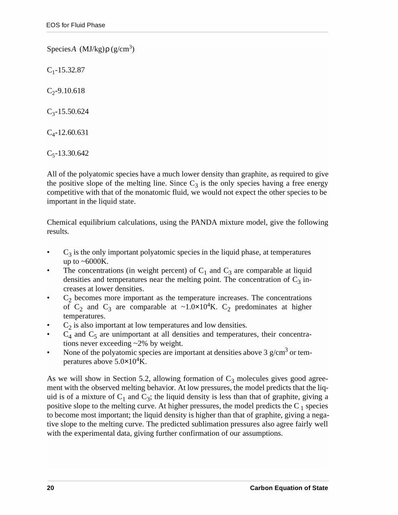
Species (MJ/kg) (g/cm3)

C1-15.32.87

C2-9.10.618

C3-15.50.624

C4-12.60.631

C5-13.30.642

All of the polyatomic species have a much lower density than graphite, as required to givethe positive slope of the melting line. Since C3 is the only species having a free energycompetitive with that of the monatomic fluid, we would not expect the other species to beimportant in the liquid state.

Chemical equilibrium calculations, using the PANDA mixture model, give the followingresults.

• C3 is the only important polyatomic species in the liquid phase, at temperaturesup to ~6000K.

• The concentrations (in weight percent) of C1 and C3 are comparable at liquiddensities and temperatures near the melting point. The concentration of C3 in-creases at lower densities.

• C2 becomes more important as the temperature increases. The concentrationsof C2 and C3 are comparable at ~1.0×104K. C2 predominates at highertemperatures.

• C2 is also important at low temperatures and low densities.• C4 and C5 are unimportant at all densities and temperatures, their concentra-

tions never exceeding ~2% by weight.• None of the polyatomic species are important at densities above 3 g/cm3 or tem-

peratures above 5.0×104K.

As we will show in Section 5.2, allowing formation of C3 molecules gives good agree-ment with the observed melting behavior. At low pressures, the model predicts that the liq-uid is of a mixture of C1 and C3; the liquid density is less than that of graphite, giving apositive slope to the melting curve. At higher pressures, the model predicts the C 1 speciesto become most important; the liquid density is higher than that of graphite, giving a nega-tive slope to the melting curve. The predicted sublimation pressures also agree fairly wellwith the experimental data, giving further confirmation of our assumptions.

A ρ


Thermal Electronic Contributions

4. Thermal Electronic Contributions

4.1 General

At sufficiently high temperatures, excitation of electrons out of the ground state configura-tion makes an important contribution to the thermodynamic properties. In this work, thethermal electronic terms for the metallic phases [subscripted e in Equations. (1)-(3) and(11)] were calculated using the PANDA ionization equilibrium model (IEQ) [18]. TheINFERNO model of Liberman [49] was also used to test the IEQ results at high densities.

The IEQ model used in this work includes two improvements to the average atom approx-imation not discussed in the PANDA manual [18]—corrections for charge fluctuationsand for thermal broadening. Therefore, we will give a brief outline of the theory and howit has been modified. (See Reference [18] for additional discussion.)

4.2 Basic Theory

We consider an element with atomic number and atomic weight . A particular config-uration of this system is specified by giving the populations of the electronic orbitals, eachorbital describing the state of a single electron. To calculate the thermodynamic propertiesof the system, it is necessary to take a thermal average over all configurations of the sys-tem, according to the principles of statistical mechanics.

The PANDA IEQ model uses an average atom approximation to the ionization equilibri-um equations. Like other average atom models, the properties of the system are computedby considering the electronic structure of a single atom. However, this model is unique inthat it explicitly sums over all electronic configurations of the atom instead of consideringa single “average” configuration. The most recent version of the model also includes cor-rections to the average atom approximation that are discussed below.

The electronic contribution to the Helmholtz free energy is given by

, (20)

where , the electronic partition function for an “average ion,” is a sum over all Z+1states of ionization,

. (21)

Z W

Ae RT W⁄( ) qeln–=

qe

qe qz δz uz zaf0 z( )+ +[ ] kT⁄–( )exp

z 0=

Z

∑=



Here is the free energy (per electron) for an electron gas in which there are z free elec-trons per ion. is the partition function and is the ground state energy for an ion ofcharge z. is a correction to the average atom model, which is discussed below.

The ion partitition function is given by

(22)

where and are the statistical weights and energy levels of the ion, and thesum is taken over all configurations of the electrons. These quantities, along with theground state energies , are calculated from a scaling model, using a table of orbital radiiand energies for the ground state configuration of the isolated atom [50], along with cor-rections for ionization and continuum lowering, as discussed in Section 9 ofReference [18].

The IEQ model generates a table of the electronic entropy as a function of density andtemperature. This table is input to the solid or liquid model. The pressure, internal energy,and Helmholtz free energy are computed from the entropy table, using standard thermody-namic relations. For density-temperature points off the table, PANDA uses the TFD mod-el. See Section 8 of Reference [18] for details.

4.3 Charge Fluctuations

The average atom corrections, in Equation (21), are new additions to the IEQ modeland are not discussed in the PANDA manual. One of the approximations in the averageatom model is that charge neutrality holds within an ion sphere. In Reference [51], weshowed that there are fluctuations in the charge within an ion sphere, and we derived ex-pressions for the corrections that are valid in the low-density limit. We showed that satis-factory results can be obtained by taking for z>1. (See Reference [51] for theexplicit formulas for and .)

We have not yet found a rigorous theory of charge fluctuations at high densities. However,the fluctuation terms are expected to become less important as the density increases, be-cause of increased attraction between “holes” and “electrons.” In order to account for thiseffect, the low-density values are modified as follows.

, (23)

where is an input parameter, typically ranging from 0.1 to 1.0. This expression wasmotivated by a model of electrical conductivity data near the metal-insulator transition[52]. A preliminary comparison with the experimental data indicates that it captures theessential features of the physics.

af0

qz uzδz

qz gz n( ) εz n( ) kT⁄–[ ]expn∑=

gz n( ) εz n( )

uz

δz

δz 0≈δ0 δ1

δz δz 150F3ρ W⁄–( )exp→

F3



4.4 Thermal Broadening

Another approximation in the average atom model is that all ion spheres are equal in size.In fact, thermal motions can lead to fluctuations in the sizes of the ion spheres. The latestversion of PANDA includes a correction for this effect.

Consider a configuration of N atoms in which the ion spheres have volumes that fluctuate about the average volume ,

. (24)

It follows that

. (25)

The energy of this configuration can be expressed in terms of volume fluctuation by ex-panding in a Taylor series about the average volume. If is the energy for a single ionsphere of volume ,

, (26)

where we have discarded terms above second-order. The energy derivative in Eq. (26) canbe expressed in terms of the bulk modulus and the sound speed, giving

, where . (27)

The statistical-mechanical average of some quantity over all configurations is

. (28)

To simplify the evaluation of the above integral, we will drop the restriction on the ionsphere volumes, Eq. (25). In that case, the integration over each sphere volume isindependent. Then

v1 v2 … vN, , ,v

v N1–

vi

i 1=

N

∑=

vi v–( )i 1=

N

∑ 0=

e vi( )vi

E e vi( )i∑ Ne v( ) 1

2--- d

2e

dv2

--------

v

vi v–( )2i∑+= =

E E kXB vi v⁄ 1–( )2i∑≈– XB Wcs

22R⁄ 60Wcs

2(Kelvin)= =

Fv1 v2 … vN, , ,

F⟨ ⟩F v1…vN( ) E E–( ) kT⁄[ ]exp v1…d vNd∫

E E–( ) kT⁄[ ]exp v1…d vNd∫-------------------------------------------------------------------------------------------------=



. (29)

Equation (29) is the thermal broadening relation that we use to average the IEQ entropy,calculated from the average atom approximation, over fluctuations in density. In practice,the principal effect of this procedure is to smooth discontinuities that arise when boundlevels are cut off due to pressure ionization. The smoothing effect is particularly importantnear the metal-insulator transition, where the ground state of the atom is pressure-ionized.

In the present version of the model, is taken to be a constant and is treated as an inputparameter. Smaller values of give more smoothing. Using the ambient sound speed forgraphite, a nominal value for carbon is 1.0×104 K. However, a much smaller value is ap-propriate in the metal-insulator transition region, where the sound speed is smaller.

4.5 Application to Carbon

In the present work, the orbital data used in the atomic scaling model were taken fromReference [50], except that the orbital binding energies EA were modified to improve theionization potentials [53] and the energies of the lowest lying excited states [16] predictedby the model. The revisions were as follows (EA in Hartree):

OrbitalEA (old)EA (mod)

1S+ -1.1389e+01 -1.1200e+01

2S+ -7.3326e-01 -7.2000e-01

2P- -3.9904e-01 -4.4000e-01

2P+ -4.4320e-01 -4.2970e-01

The IEQ results were generated using the following parameter settings.

• MX=EFAC=3. MX is the maximum number of electron-hole excitations from theground state, and EFAC is the energy cutoff, relative to the ionization energy, in thesum over excited states. These factors are large enough to include all important contri-butions to the ion partition functions.

• F1=F2=1. We chose the default values for these factors, which are used in thecontinuum-lowering model, because they gave good agreement with the density of themetal-insulator transition obtained using the INFERNO model [49].

• F3=0.1. This constant, used in the average atom corrections, Equation (23), was thesame as we have used in calculations for other metals [52].

• XB=1.0×10-3K. This constant, used in the thermal broadening model, Eq. (29), waschosen to get a reasonable amount of smoothing.

The entropy was computed at 63 densities, , and at 36temperatures, . (The T=0 points were obtained by extrapolation.)

F⟨ ⟩ F v( ) XB v v⁄ 1–( )2T⁄–[ ]exp vd∫ XB v v⁄ 1–( )2

T⁄–[ ]exp vd∫⁄≈

XBXB

1.0 10 10–× ρ 1.0 103× g/cc≤ ≤0 T 1.16 10

8× K≤ ≤



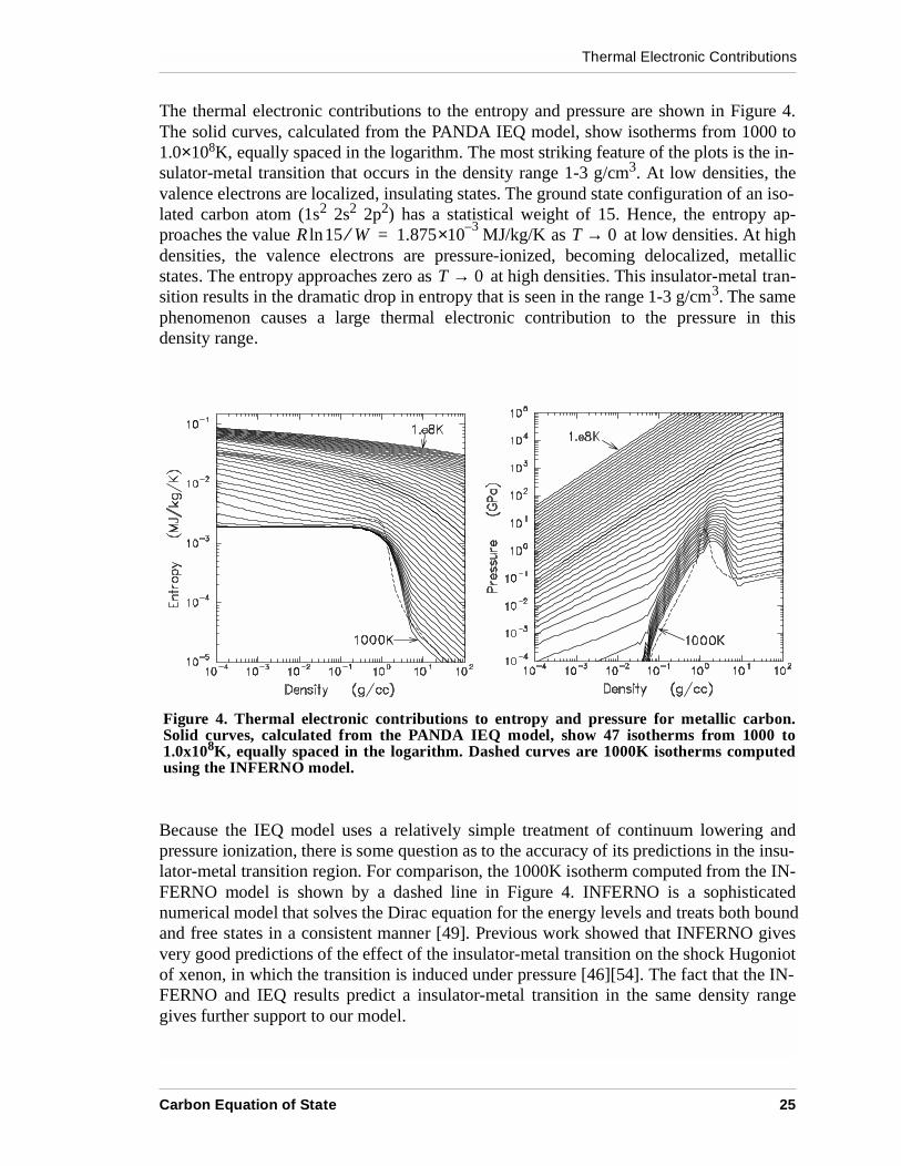
The thermal electronic contributions to the entropy and pressure are shown in Figure 4.The solid curves, calculated from the PANDA IEQ model, show isotherms from 1000 to1.0×108K, equally spaced in the logarithm. The most striking feature of the plots is the in-sulator-metal transition that occurs in the density range 1-3 g/cm3. At low densities, thevalence electrons are localized, insulating states. The ground state configuration of an iso-lated carbon atom (1s2 2s2 2p2) has a statistical weight of 15. Hence, the entropy ap-proaches the value as at low densities. At highdensities, the valence electrons are pressure-ionized, becoming delocalized, metallicstates. The entropy approaches zero as at high densities. This insulator-metal tran-sition results in the dramatic drop in entropy that is seen in the range 1-3 g/cm3. The samephenomenon causes a large thermal electronic contribution to the pressure in thisdensity range.

Because the IEQ model uses a relatively simple treatment of continuum lowering andpressure ionization, there is some question as to the accuracy of its predictions in the insu-lator-metal transition region. For comparison, the 1000K isotherm computed from the IN-FERNO model is shown by a dashed line in Figure 4. INFERNO is a sophisticatednumerical model that solves the Dirac equation for the energy levels and treats both boundand free states in a consistent manner [49]. Previous work showed that INFERNO givesvery good predictions of the effect of the insulator-metal transition on the shock Hugoniotof xenon, in which the transition is induced under pressure [46][54]. The fact that the IN-FERNO and IEQ results predict a insulator-metal transition in the same density rangegives further support to our model.

R 15 W⁄ln 1.8753–×10 MJ/kg/K= T 0→

T 0→

Figure 4. Thermal electronic contributions to entropy and pressure for metallic carbon.Solid curves, calculated from the PANDA IEQ model, show 47 isotherms from 1000 to1.0x108K, equally spaced in the logarithm. Dashed curves are 1000K isotherms computedusing the INFERNO model.



However, there are two differences between INFERNO and IEQ that should be noted.First, INFERNO gives a higher entropy than IEQ at low densities. The INFERNO result isincorrect at low densities because of an error introduced by the average configuration ap-proximation, as explained in Reference [51]. Second, INFERNO predicts a sharper drop inentropy at the transition because it does not include any thermal broadening. For these rea-sons, we consider IEQ to be the more accurate model for carbon, even though it uses amore simplified treatment of continuum lowering and pressure ionization.

Finally, we note that the above results support our assumption that liquid carbon is metal-lic at densities above about 3 g/cm3. At lower densities, the transition seen in the electron-ic structure, along with the formation of molecular species in the liquid state, could beresponsible for the observed drop in thermal conductivity [14].


Results and Discussion

5. Results and Discussion

5.1 Multiphase EOS Calculations

The PANDA MOD MIX option was used to construct a single EOS table for a fluid phasemixture of C1, C2, and C3. (C4 and C5 were not included in the final EOS because theywere found to be unimportant, as discussed in Section 3.4.) In order to eliminate numericalproblems in the mixture model, it was necessary to include Maxwell constructions in theEOS tables for the various species.

Next, the PANDA MOD TRN option was used to compute the phase diagram and con-struct the multiphase EOS, including four phases—graphite, diamond, metallic solid, andthe fluid mixture. The “imperfect” form of diamond was used in making the EOS table, inorder to match the shock data as discussed below.

The mesh used in making the multiphase EOS table included 84 densities in the range, plus a point, and 74 temperatures in the range

. The mesh points were chosen to give good resolution of the phase tran-sitions and other important features of the EOS surface. In order to allow treatment offracture models, a tension region was included at temperatures below the sublimationpoint (TSPALL=3600). Maxwell constructions were included at all higher temperatures,as noted above.

The new EOS table has been added to the SNL-SESAME library (file “sesame”) as mate-rial number 7830.

5.2 Equilibrium Phase Diagram

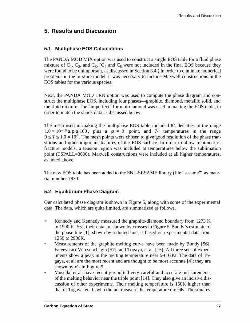
Our calculated phase diagram is shown in Figure 5, along with some of the experimentaldata. The data, which are quite limited, are summarized as follows.

• Kennedy and Kennedy measured the graphite-diamond boundary from 1273 Kto 1900 K [55]; their data are shown by crosses in Figure 5. Bundy’s estimate ofthe phase line [1], shown by a dotted line, is based on experimental data from1250 to 2900K.

• Measurements of the graphite-melting curve have been made by Bundy [56],Fateeva and Vereschchagin [57], and Togaya, et al. [15]. All three sets of exper-iments show a peak in the melting temperature near 5-6 GPa. The data of To-gaya, et al. are the most recent and are thought to be most accurate [4]; they areshown by x’s in Figure 5.

• Musella, et al. have recently reported very careful and accurate measurementsof the melting behavior near the triple point [14]. They also give an incisive dis-cussion of other experiments. Their melting temperature is 150K higher thanthat of Togaya, et al., who did not measure the temperature directly. The squares

1.0 10 10–× ρ 100≤ ≤ ρ 0=0 T 1.0 108×≤ ≤



in Figure 5 show the point of Musella, et al., together with the data of Togaya, etal., shifted by +150K.

• The diamond melting line has not been measured directly. However, it is cur-rently thought that the phase boundary has a positive slope, based on soundspeed measurements of Shaner, et al. [58][59]. We will discuss those experi-ments in Section 5.5.

As seen in Figure 5, our calculated phase diagram agrees quite well with the existing data.Our graphite-diamond boundary deviates slightly from Bundy’s extrapolation [1] at hightemperatures. The reason is that his extrapolation assumes a constant difference in heat ca-pacity between graphite and diamond. Our model, which uses a more sophisticated treat-ment of the lattice vibrational terms, does not make that assumption.

Our calculated melting curve shows the observed behavior—a positive slope at low pres-sures, a maximum near 5 GPa, and a negative slope at high pressures. As noted in Section3.3, one of the parameters in the liquid model (EFAC) was adjusted to match the high-pressure behavior. We chose to match the data of Togaya, et al., shifted by +150K. Thecalculated phase line is within the uncertainties in the experimental data.

The formation of polyatomic molecules, especially C3, plays an essential role in matchingthe distinctive character of the graphite-melting curve. The dashed line in Figure 5 showsthe melting curve obtained when only the monatomic species C1 is allowed to form. Inthat case, the melting curve has a negative slope at all pressures up to the graphite-diamond-liquid triple point. Formation of the polyatomic molecules lowers the density ofthe liquid phase and gives a positive slope at low pressures, in agreement with the ob-served behavior.

Figure 5. Phase diagram forcarbon. Experimental data:crosses [55]; dotted curve [1](extrapolation above 2900K); x’s[15]; squares [14], and data of [15],shifted by +150K. The solid curvesare our calculated boundaries. Thedashed curve is the calculatedmelting curve when molecularspecies are excluded from theliquid phase.



Our model predicts a graphite-liquid-vapor triple point at 0.017 GPa and 4660K, close tothe recent measurements of Musella, et al. (0.011±0.002 GPa and 4800±150K [14]). Oursublimation point is 3800K, in satisfactory agreement with other work [16][60].

5.3 Melting Data

Because it is very difficult to perform experiments on liquid carbon [14], there are no pre-cise measurements of the enthalpy and density changes at the melting point. Baitin, et al.,estimated the enthalpy of fusion to be 10.4 MJ/kg, using the exploding wire technique[61]. Musella, et al., estimated a 45% volume change on melting, based upon the void vol-ume obtained in recovered melted samples [14].

The isobaric expansion experiments of Gathers, et al. [62], also provide some informationabout the melting behavior. Glassy carbon samples, kept at constant pressure by a neutralgas, were resistively heated. The current-voltage data were used to determine the enthalpyas a function of time. The density was determined as a function of time from streak camerameasurements of the sample diameter.

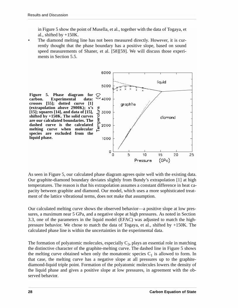
Figure 6 shows the measured enthalpy vs.density for samples at 0.2 and 0.4 GPa. Thesamples had an initial density of 1.83 g/cm3. On heating, the samples first expandslightly, then contract to near the theoreti-cal density at an enthalpy of 7 MJ/kg,which corresponds to a temperature near4000K, below the melting point.

Our calculations of the isobaric experi-ments are compared with the data inFigure 6. (Since the calculations were madefor nonporous graphite, only the resultsabove 7 MJ/kg should be compared withthe data.) According to our model, meltingoccurs at an enthalpy of about 9 MJ/kg.There is a sharp change in slope as the sam-ples enter the mixed phase region, shownby dotted lines. Melting is complete atabout 21 MJ/kg, which corresponds to theupper end of the measurements. The calcu-lated enthalpy of fusion is 12 MJ/kg. The calculated density change is 50%.

It should be noted that the parameter in the model for the polyatomic species(Section 3.4) was chosen to agree with these isobaric data. It may be that forcing suchgood agreement is not justified by the errors and uncertainties in the experimental

Figure 6. Isobaric expansion data forcarbon. Experimental data: circles—0.2GPa, squares—0.4 GPa. Curves arecalculated from our model, the dottedportions showing the mixed phase region.

ρ0



technique. However, the choice we have made is reasonably consistent with the data avail-able at the present time.

5.4 Nonequilibrium Behavior

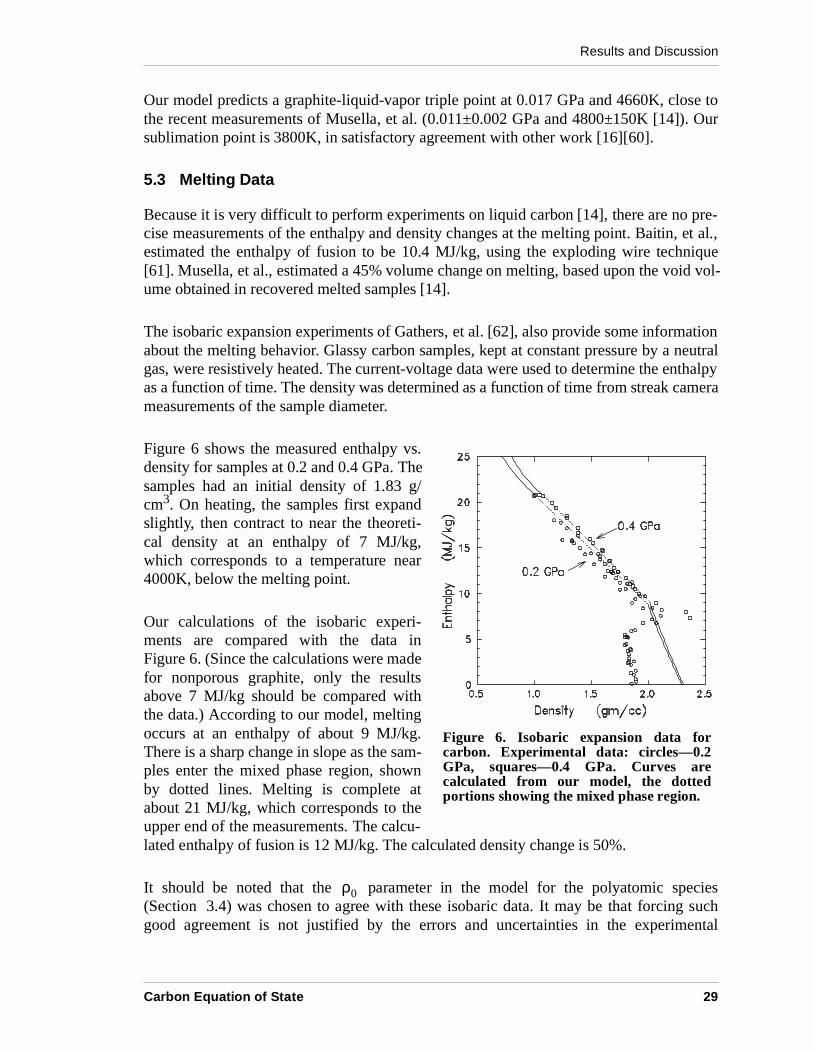
As we have already observed, the transition from graphite to diamond does not occur atthe equilibrium pressure under shock loading conditions. Many aspects of this nonequilib-rium behavior can be described by treating diamond as an imperfect crystal. Our model(Section 2.4) treats this imperfect form of diamond as a crystal containing vacant sites.Because the energy required to create a vacancy is large, compared with the free energydifference between graphite and diamond, creation of 3% vacant sites shifts the transitionpressure by an order of magnitude.

Figure 7 compares the equilibrium and nonequilibrium phase diagrams. In the equilibriumcase, shown by solid curves, the transition from diamond to the metallic solid occurs at apressure of 900 GPa at zero temperature. Because the metallic solid is denser than dia-mond (see Figure 1), the phase line has a negative slope, terminating at the melting curve.The diamond-metal-liquid triple point occurs at 220 GPa and 5400K.

The dashed lines in Figure 7 show howthe phase boundaries shift when diamondis replaced by its imperfect form. The di-amond field of stability is substantiallyreduced. The graphite-diamond transitionpressure is increased, while the diamond-metal transition pressure drops signifi-cantly. In addition, the metallic solid be-comes more stable than diamond at hightemperatures, so that diamond does notintersect the melting curve at any pres-sure. (This possibility was considered byGrover in his sensitivity studies of thecarbon phase diagram [63].)

As we will show below, this nonequilibri-um phase diagram is consistent with theavailable shock wave data for carbon.

Figure 7. Comparison of phase diagrams forcarbon. Solid curves—equilibrium phaselines. Dashed curves—phase lines obtainedwith an “imperfect” diamond phasecontaining 3% vacancies.



5.5 Shock-Wave Behavior

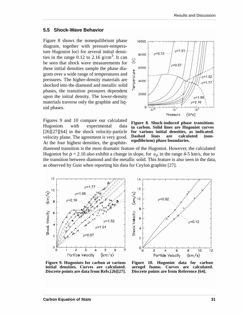
Figure 8 shows the nonequilibrium phasediagram, together with pressure-tempera-ture Hugoniot loci for several initial densi-ties in the range 0.12 to 2.16 g/cm3. It canbe seen that shock wave measurements forthese initial densities sample the phase dia-gram over a wide range of temperatures andpressures. The higher-density materials areshocked into the diamond and metallic solidphases, the transition pressures dependentupon the initial density. The lower-densitymaterials traverse only the graphite and liq-uid phases.

Figures 9 and 10 compare our calculatedHugoniots with experimental data[26][27][64] in the shock velocity-particlevelocity plane. The agreement is very good.At the four highest densities, the graphite-diamond transition is the most dramatic feature of the Hugoniot. However, the calculatedHugoniot for ρ = 2.16 also exhibit a change in slope, for in the range 4-5 km/s, due tothe transition between diamond and the metallic solid. This feature is also seen in the data,as observed by Gust when reporting his data for Ceylon graphite [27].

Figure 8. Shock-induced phase transitionsin carbon. Solid lines are Hugoniot curvesfor various initial densities, as indicated.Dashed lines are calculated (non-equilibrium) phase boundaries.

uP

Figure 9. Hugoniots for carbon at variousinitial densities. Curves are calculated.Discrete points are data from Refs.[26][27].

Figure 10. Hugoniot data for carbonaerogel foams. Curves are calculated.Discrete points are from Reference [64].



As expected from Figure 8, the lower-density carbon Hugoniots does not exhibit thegraphite-diamond phase transition. However, they do exhibit changes in slope that are dueto the melting of graphite. This feature is especially evident in the data for ρ = 1.01 for in the range 4-5 km/s.

Figure 10 shows Hugoniot data for special low-density carbon foams called “aerogels”[64]. These data also extend to higher velocities than those in Figure 9. Except for the twolowest pressure points for ρ = 0.92, all of these data lie in the fluid region. The shock tem-peratures are also quite high, up to 1.5×104K at the highest pressures, where thermal elec-tronic excitations make the most important contribution to the EOS. Our model gives verygood results for these aerogel foams, just as it does for other types of carbon.

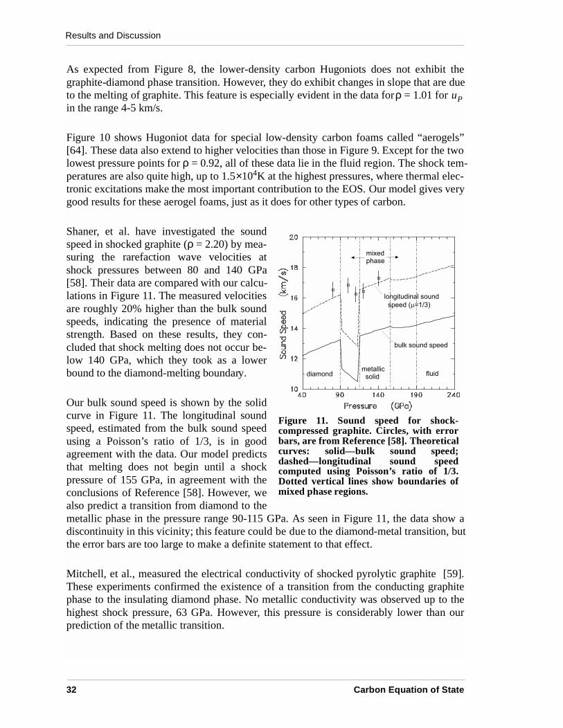
Shaner, et al. have investigated the soundspeed in shocked graphite (ρ = 2.20) by mea-suring the rarefaction wave velocities atshock pressures between 80 and 140 GPa[58]. Their data are compared with our calcu-lations in Figure 11. The measured velocitiesare roughly 20% higher than the bulk soundspeeds, indicating the presence of materialstrength. Based on these results, they con-cluded that shock melting does not occur be-low 140 GPa, which they took as a lowerbound to the diamond-melting boundary.

Our bulk sound speed is shown by the solidcurve in Figure 11. The longitudinal soundspeed, estimated from the bulk sound speedusing a Poisson’s ratio of 1/3, is in goodagreement with the data. Our model predictsthat melting does not begin until a shockpressure of 155 GPa, in agreement with theconclusions of Reference [58]. However, wealso predict a transition from diamond to themetallic phase in the pressure range 90-115 GPa. As seen in Figure 11, the data show adiscontinuity in this vicinity; this feature could be due to the diamond-metal transition, butthe error bars are too large to make a definite statement to that effect.

Mitchell, et al., measured the electrical conductivity of shocked pyrolytic graphite [59].These experiments confirmed the existence of a transition from the conducting graphitephase to the insulating diamond phase. No metallic conductivity was observed up to thehighest shock pressure, 63 GPa. However, this pressure is considerably lower than ourprediction of the metallic transition.

uP

Figure 11. Sound speed for shock-compressed graphite. Circles, with errorbars, are from Reference [58]. Theoreticalcurves: solid—bulk sound speed;dashed—longitudinal sound speedcomputed using Poisson’s ratio of 1/3.Dotted vertical lines show boundaries ofmixed phase regions.



5.6 Shock Vaporization

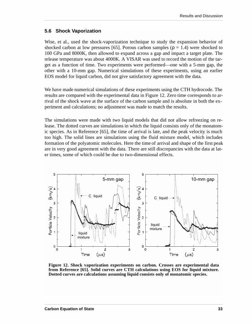
Wise, et al., used the shock-vaporization technique to study the expansion behavior ofshocked carbon at low pressures [65]. Porous carbon samples (ρ = 1.4) were shocked to100 GPa and 8000K, then allowed to expand across a gap and impact a target plate. Therelease temperature was about 4000K. A VISAR was used to record the motion of the tar-get as a function of time. Two experiments were performed—one with a 5-mm gap, theother with a 10-mm gap. Numerical simulations of these experiments, using an earlierEOS model for liquid carbon, did not give satisfactory agreement with the data.

We have made numerical simulations of these experiments using the CTH hydrocode. Theresults are compared with the experimental data in Figure 12. Zero time corresponds to ar-rival of the shock wave at the surface of the carbon sample and is absolute in both the ex-periment and calculations; no adjustment was made to match the results.

The simulations were made with two liquid models that did not allow refreezing on re-lease. The dotted curves are simulations in which the liquid consists only of the monatom-ic species. As in Reference [65], the time of arrival is late, and the peak velocity is muchtoo high. The solid lines are simulations using the fluid mixture model, which includesformation of the polyatomic molecules. Here the time of arrival and shape of the first peakare in very good agreement with the data. There are still discrepancies with the data at lat-er times, some of which could be due to two-dimensional effects.

Figure 12. Shock vaporization experiments on carbon. Crosses are experimental datafrom Reference [65]. Solid curves are CTH calculations using EOS for liquid mixture.Dotted curves are calculations assuming liquid consists only of monatomic species.




Conclusions and Recommendations

6. Conclusions and Recommendations

We have developed a new tabular equation of state for carbon, which includes treatment ofsolid-solid phase transitions, melting, vaporization, chemical reactions, and thermal elec-tronic excitation. The EOS is in good agreement with experimental thermophysical data,static compression data, phase boundaries, and shock-wave measurements.

The new EOS table has been added to the SNL-SESAME library as material number 7830and is available for use in calculations using CTH and other hydrocodes. This EOS coverssuch a wide range of densities (0 - 100 g/cm3) and temperatures (0 - 1.0×108K) that itshould be suitable for virtually any standard hydrocode problem. It is applicable to porouscarbon materials, including aerogels, as well as denser forms.

The new EOS will also play an important role in developing improved EOS tables for avariety of other materials containing carbon—explosive detonation products, the reactionproducts of plastics, polymers, and organic substances, and carbon composites.

We believe that this new EOS is a significant improvement in the modeling of carbon andmaterials containing carbon. However, there are still many issues that deserve additionalinvestigation. In particular, new experimental data on the melting behavior and propertiesof the liquid would be useful to improve the calibration of certain model parameters. Ad-ditional experimental and theoretical work on the properties of polyatomic carbon mole-cules in the liquid phase would be desirable. Finally, development of a time-dependentmodel of the graphite-diamond transition and other nonequilibrium behavior would be anoteworthy achievement.


Conclusions and Recommendations


References

References

[1] F. P. Bundy, ‘‘The P,T Phase and Reaction Diagram for Elemental Carbon, 1979,’’ J.Geophys. Res. 85, 6930-6936 (1980).

[2] P. Gustafson, “An Evaluation of the Thermodynamic Properties and the P,T PhaseDiagram of Carbon,” Carbon 24, 169-176 (1986).

[3] F. P. Bundy, ‘‘Pressure-Temperature Phase Diagram for Elemental Carbon,’’ PhysicaA 156, 169-178 (1989).

[4] F. P. Bundy, W. A. Bassett, M. S. Weathers, R. J. Hemley, H. K. Mao, and A. F. Gon-charov, “The Pressure-Temperature Phase and Transformation Diagram for Carbon;Updated Through 1994,” Carbon 34, 141-153 (1996).

[5] L. Pauling, The Nature of the Chemical Bond (Cornell University Press, Ithaca, N.Y., 1960) 3rd. Ed.

[6] O. L. Blakslee, D. G. Proctor, E. J. Seldin, G. B. Spence, and T. Weng, ‘‘Elastic Con-stants of Compression-Annealed Pyrolytic Graphite,’’ J. Appl. Phys. 41, 3373-3389(1970).

[7] W Krätschmer, L. D. Lamb, K. Fostiropoulos, and D. R. Huffman, “Solid C60: ANew Form of Carbon,” Nature 347, 354-358 (1990).

[8] B. E. Warren, “X-Ray Diffraction in Random Layer Lattices,” Phys. Rev. 59, 693-698 (1941).

[9] J. Robertson, ‘‘Amorphous Carbon,’’ Adv. Phys. 35, 317-374 (1987).

[10] S. K. Das and E. E. Hucke, ‘‘Experimental Measurements on Configurational FreeEnergy Change of the Graphite-Glassy Carbon Equilibrium,’’ Carbon 13, 33-41(1975).

[11] G. I. Kerley, ‘‘Theoretical Equations of State for the Detonation Properties of Explo-sives,'' in Proceedings of the Eighth Symposium (International) on Detonation, edit-ed by J. M. Short, NSWL MP 86-194 (Naval Surface Weapons Center, White Oak,MD, 1986), pp. 540-547.

[12] G. I. Kerley, ‘‘Theoretical Model of Explosive Detonation Products: Tests and Sensi-tivity Studies,'' in Proceedings of the Ninth Symposium (International) on Detona-tion, edited by W. J. Morat, OCNR 113291-7 (Office of the Chief of Naval Research,1990), pp. 443-451.

[13] G. I. Kerley and T. L. Christian-Frear, “Prediction of Explosive Cylinder Tests UsingEquations of State from the PANDA Code,” Sandia National Laboratories reportSAND93-2131, 1993.


References

[14] M. Musella, C. Ronchi, M. Brykin, and M. Sheindlin, “The Molten State of Graph-ite: An Experimental Study,” J. Appl. Phys. 84, 2530-2537 (1998).

[15] M. Togaya, S. Sugiyama, and E. Mizuhara, “Melting Line of Graphite,” in HighPressure Science and Technology - 1993, edited by S. C. Schmidt, J. W; Shaner, G.A. Samara, and M. Ross (AIP Conference Proceedings 309, 1994) pp. 255-258.

[16] M. W. Chase, Jr., C. A. Davies, J. R. Downey, Jr., D. J. Frurip, R. A. McDonald, andA. N. Syverud, “JANAF Thermochemical Tables,” J. Phys. Chem. Reference Data14, Supp. No. 1 (1985).

[17] K. S. Pitzer and E. Clementi, ‘‘Large Molecules in Carbon Vapor,’’ J. Am. Chem.Soc. 81, 4479-4485 (1959).

[18] G. I. Kerley, “User’s Manual for PANDA II: A Computer Code for CalculatingEquations of State,” Sandia National Laboratories report SAND88-2291, 1991.

[19] J. M. McGlaun, F. J. Ziegler, S. L. Thompson, L. N. Kmetyk, and M. G. Elrick,“CTH - User's Manual and Input Instructions,” Sandia National Laboratories reportSAND88-0523, April 1988.

[20] J. M. McGlaun, S. L. Thompson, and M. G. Elrick, “CTH: A Three-DimensionalShock Wave Physics Code,” Int. J. Impact Engng. 10, 351-360 (1990).

[21] J. M. McGlaun, S. L. Thompson, L. N. Kmetyk, and M. G. Elrick, “A Brief Descrip-tion of the Three-Dimensional Shock Wave Physics Code CTH,” Sandia NationalLaboratories report SAND89-0607, July 1990.

[22] E. S. Hertel, Jr. and G. I. Kerley, “CTH EOS Package: Introductory Tutorial,” SandiaNational Laboratories report SAND98-0945, 1998.

[23] E. S. Hertel, Jr. and G. I. Kerley, “CTH Reference Manual: The Equation of StatePackage,” Sandia National Laboratories report SAND98-0947, 1998.

[24] B. K. Godwal, S. K. Sikka, and R. Chidambaram, “Equation of State Theories ofCondensed Matter Up To About 10 TPa,” Phys. Rep. 102, 121-197 (1983).

[25] M. Hanfland, H. Beister, and K. Syassen, ‘‘Graphite Under Pressure: Equation-of-State and First-Order Raman Modes,’’ Phys. Rev. B 39, 12598-12603 (1989).

[26] S. P. Marsh, LASL Shock Hugoniot Data (University of California Press, Berkeley,1980).

[27] W. H. Gust, ‘‘Phase Transition and Shock-Compression Parameters to 120 GPa forThree Types of Graphite and for Amorphous Carbon,’’ Phys. Rev. B 22, 4744-4756(l980).


References

[28] D. J. Erskine and W. J. Nellis, “Shock-Induced Martensitic Transformation of Ori-ented Graphite to Diamond,” Nature, Vol. 349, 317-319 (1991).

[29] D. J. Erskine and W. J. Nellis, “Shock-Induced Martensitic Transformation of High-ly Oriented Graphite to Diamond,” J. Appl. Phys. 71, 4882-4886 (1992).

[30] I. V. Aleksandrov, A. F. Goncharov, A. N. Zisman, and S. M. Stishov, ‘‘Diamond atHigh Pressures: Raman Scattering of Light, Equation of State, and High-PressureScale,’’ Sov. Phys. JETP 66, 384-390 (1988).

[31] R. Al-Jishi and G. Dresselhaus, “Lattic-Dynamical Model for Graphite,” Phys. Rev.B 26, 4514-4522 (1982).

[32] Y. S. Touloukian, R. K. Kirby, R. E. Taylor, and T. Y. R. Lee, ‘‘Thermal Expansion,Nonmetallic Solids,’’ Thermophysical Properties of Matter (IFI/Plenum, New York,1977) Vol. 13.

[33] R. Hultgren, P. D. Desai, D. T. Hawkins, M. Gleiser, K. K. Kelley, and D. D. Wag-man, Selected Values of the Thermodynamic Properties of the Elements (AmericanSociety for Metals, Metals Park, Ohio, 1972).

[34] S. Fahy and S. G. Louie, ‘‘High-Pressure Structural and Electronic Properties ofCarbon,’’ Phys. Rev. B 36, 3373-3385 (1987).

[35] J. F. Cannon, “Behavior of the Elements at High Pressures,” J. Phys. Chem. Refer-ence Data 3, 781-824 (1974).

[36] H. J. McSkimin and P. Andreatch, Jr., “Elastic Moduli of Diamond as a Function ofPressure and Temperature,” J. Appl. Phys. 43, 2944-2948 (1972).

[37] See, for example, C. Kittel, Introduction to Solid State Physics (Wiley, New York,1963), 2nd Ed., pp 122-125.

[38] M. Hanfland, K. Syassen, S. Fahy, S. G. Louie, and M. L. Cohen, ‘‘Pressure Depen-dence of the First-Order Raman Mode in Diamond,’’ Phys. Rev. B 31, 6896-6899(1985).

[39] Handbook of Chemistry and Physics, edited by David R. Lide (CRC Press, Boca Ra-ton, 1996) 77th edition.

[40] M. T. Yin and M. L. Cohen, “Will Diamond Transform under Megabar Pressures?”Phys. Rev. Lett. 50, 2006 (1983).

[41] R. Biswas, R. M. Martin, R. J. Needs, and O. H. Nielsen, “Complex TetrahedralStructures of Silicon and Carbon under Pressure,” Phys. Rev. B 30, 3210-3213(1984).


References

[42] A. Y. Liu, M. L. Cohen, K. C. Hass, and M. A. Tamor, “Structural Properties of aThree-Dimensional All-sp2 Phase of Carbon,” Phys. Rev. B 43, 6742-6745 (1991).

[43] A. Y. Liu and M. L. Cohen, “Theoretical Study of a Hypothetical Metallic Phase ofCarbon,” Phys. Rev. B 45, 4579-4581 (1992).

[44] G. I. Kerley, “Multiphase Equation of State for Iron,” Sandia National Laboratoriesreport SAND93-0027, 1993.

[45] G. I. Kerley, “Perturbation Theory and the Thermodynamic Properties of Fluids II.The CRIS Model,” J. Chem. Phys. 73, 478-486 (1980).

[46] G. I. Kerley, “A Model for the Calculation of Thermodynamic Properties of a FluidUsing Hard-Sphere Perturbation Theory and the Zero-Kelvin Isotherm of the Solid,''in Molecular Based Study of Fluids, edited by J. M. Haile and G. A. Mansoori (Am.Chem. Soc., Washington, DC., 1983) pp. 107-138.

[47] J. H. Rose, J. R. Smith, F. Guinea, and J. Ferrante, “Universal Features of the Equa-tion of State of Metals,” Phys. Rev. B 29, 2963-2969 (1984).

[48] L. A. Girifalco and R. A. Lad, “Energy of Cohesion, Compressibility, and the Poten-tial Energy Functions of the Graphite System,” J. Chem. Phys. 25, 693-697 (1956).

[49] D. A. Liberman, “Self-Consistent Field Model for Condensed Matter,” Phys. Rev. B20, 4981-4989 (1979).

[50] G. I. Kerley, “Atomic Orbital Data for Elements with Atomic Numbers 1 ≤ Z ≤ 103,”Sandia National Laboratories report SAND88-2594, 1988.

[51] G. I. Kerley, “Theory of Ionization Equilibrium: An Approximation for the SingleElement Case,” J. Chem. Phys. 85, 5228-5231 (1986).

[52] G. I. Kerley, “Modification of the Lee-More Conductivity Model: Improved Calcu-lation of Ionization State,” Kerley Publishing Services report KPS99-2, Albuquer-que, NM, February 1999.

[53] R. D. Cowan, The Theory of Atomic Structure and Spectra (University of California,Berkeley, 1981) pp. 12-15.

[54] G. I. Kerley, “Theoretical Model of Liquid Metals,” in Proceedings of the EighthSymposium on Thermophysical Properties, J. V. Sengers (Ed.) (Am. Soc. Mech. En-gineers, New York, NY, 1982) Vol II, pp. 159-164.

[55] C. S. Kennedy and G. C. Kennedy, “The Equilibrium Boundary Between Graphiteand Diamond,” J. Geophys. Res. 81, 2467-2470 (1976).

[56] F. P. Bundy, “Melting of Graphite at Very High Pressure,” J. Chem. Phys. 38,618-630 (1963).


References

[57] N. S. Fateeva and L. F. Vereshchagin, “Concerning the Melting Point of Graphite upto 90 kbar,” JETP Lett. 13, 110-111 (1971).

[58] J. W. Shaner, J. M. Brown, C. A. Swenson, and R. G. McQueen, “Sound Velocity ofCarbon at High Pressures,” J. de Physique 45, C8235-237 (1984).

[59] A. C. Mitchell, J. W. Shaner, and R. N. Keeler, “The Use of Electrical ConductivityExperiments to Study the Phase Diagram of Carbon,” Physica 139, 386-389 (1986).

[60] H. B. Palmer, “On the Equilibrium Vapor Pressure of Graphite and the Temperatureof the Carbon Arc,” Carbon 8, 243-244 (1970).

[61] A. V. Baitin, A. A. Levedev, S. V. Romanenko, V. N. Senchenko, and M. A. Schend-lin, “The Melting Point and Optical Properties of Solid and Liquid Carbon at Pres-sures of Up to 2 kbar,” High Temp. - High Pres. 21, 157-170 (1990).

[62] G. R. Gathers, J. W. Shaner, and D. W. Young, “High-Temperature Carbon Equationof State,” Lawrence Livermore Laboratory report UCRL-51644, September 14,1974.

[63] R. Grover, “Does Diamond Melt?,” J. Chem. Phys. 71, 3824-3829 (1979).

[64] N. C. Holmes, “Shock Compression of Low-Density Foams,” in High Pressure Sci-ence and Technology - 1993, edited by S. C. Schmidt, J. W; Shaner, G. A. Samara,and M. Ross (AIP Conference Proceedings 309, 1994) pp. 153-156.

[65] J. L. Wise, G. I. Kerley, and T. G. Trucano, ‘‘Shock-Vaporization Studies on Zincand Porous Carbon,'' in Shock Waves in Condensed Matter - 1991, edited by S. C.Schmidt, R. D. Dick, J. W. Forbes, and D. G. Tasker (Elsevier, 1992) pp. 61-64.


References


Distribution

Distribution

1 General Dynamics Electric Boat DivisionAttn: Chris Abate, MS D5-47500 Eastern Point RoadGroton, CT 06340-4989

1 New Mexico TechAttn: Robert Abernathy, EMRTCSocorro, NM 87801

1 USAE Waterways Experiment StationAttn: Mark D.Adley3909 Halls Ferry RoadVicksburg, MI 39180-6199

1 California Institute of TechnologySeismological Laboratory 252-21Attn: Thomas J.AhrensPasadena, CA 91125

1 Southwest Research InstituteAttn: Charles E.AndersonP. O. Drawer 28510San Antonio, TX 78228-0510

4 Applied Research Associates, IncAttn: D. E. Grady B. L. Bingham C. Scheffield4300 San Mateo Blvd. NE, Suite A-220Albuquerque, NM 87110

4 Applied Research AssociatesAttn: P. T. Dzwilewski

K. EdquistL. BrownG. Recht

5941 South Middlefield Rd., Suite 100Littleton, CO 80123

1 Kaman Sciences CorporationAttn: Nasit AriP. O. Box 7463Colorado Springs, CO 80933

1 USAE Waterways Experiment StationAttn: Byron J. Armstrong3909 Halls Ferry RdVicksburg, MS 39180

1 U. S. Army ARDECSMCAR-AEE-WWAttn:Ernest L. BakerPicatinny Arsenal, NJ 07806-5000

1 Institute for Defense AnalysesAttn:Bohdan Balko1801 North Beauregard StreetAlexandria, VA 22311

1 Lockheed Martin Launching SystemsVLS Loading DockAttn:Larry Barisciano103 Chesapeake Park PlazaBaltimore, MD 21220-0931

1 Applied Physics LabAttn:Olivier Barnouin-JhaJohn Hopkins RoadLaurel, MD 20723-6099

1 USAE Waterways Experiment StationAttn: Tommy Bevins3909 Halls Ferry RdVicksburg, MS 39180

1 Commander: U.S. Army TACOMAMSTA-TR-R MS 263Attn:Krishan D. BishnoiWarren, MI 48397-5000

1 The University of Texas at AustinInstitute for Advanced TechnologyAttn:Stephan J. Bless4030-2 W. Braker Lane, Suite 200Austin, TX 78712

1 Wright LaboratoryWL/MNSAAttn:Dan BrubakerEglin AFB, FL 32542-5434

1 Hughes Missile Systems Co.Attn:David CampbellBldg 805 MS C4PO Box 11337Tucson AZ, 85734

1 Teledyne Brown EngineeringAttn:Burton S. Chambers IIIM/S 66PO Box 070007Huntsville, AL 35807-7007


Distribution

1 Aerojet Propulsion DivisionAttn: Bounmy Chhouk

Department 5215P.O. Box 13222Sacramento, CA 95813-6000

1 U. S. Army ARDECSMCAR-AEE-WW - Bldg. 3022Attn: Chuck ChinPicatinny Arsenal, NJ 07806-5000

1 NASA Johnson Space CenterAttn: Eric L. ChristiansenMail Code SN3Houston, TX 77058

1 Lockheed Martin Idaho Tech - INELAttn: Henry Chu

M/S 0206P.O. Box 1625Idaho Falls, ID 83415-0206

1 Thiokol CorporationScience & Engineering DivisionAttn: Dwight ClarkMailstop 280P. O. Box 707Brigham City, Utah 84302-0707

1 MEVATECAttn: Steve Clark1525 Perimeter Parkway, Suite 500Huntsville, AL 35806

1 DynaEast CorporationAttn: William Clark3620 Horizon DriveKing of Prussia, PA 19104

1 Talley Defense SystemsAttn: Jon ConnerP.O. Box 849Mesa, Arizona 85211

1 Wright LaboratoryWL/MNMW Bldg. 13Attn: William CookEglin AFB, FL 32542-5434

1 DominicaAttn: Nancy Winfree9813 Admiral DeweyAlbuquerque, NM 87111

1 U. S. Army Natick Research and Development CenterSATNC-IBAttn:Philip CunniffKansas StreetNatick, MA 01760-5019

1 University of IllinoisNCSAAttn:LeRay DandyUrbana Champaign, IL

1 TASC, Inc.Attn:Charles Drutman5500 Walkers Brook DriveReading, MA 01940

1 The Ensign-Bickford CompanyAttn:Kevin Duprey660 Hopmeadow StreetSimsbury, CT 06070-0483

1 Advatech Pacific Inc.Attn: Jay EbersohlPO Box 1376San Bernardino, CA 92402-1376

1 Foils EngineeringAttn:Marshall B. Eck25731 Ridge RoadDamascus, MD 20872

1 Enig Associates, Inc.Attn: Julius W. Enig11120 New Hampshire Ave., Suite 500Silver Spring, MD 20904-2633

1 General DynamicsAttn: James EridonMail Zone 439-01-07P. O. Box 2094Warren, MI 48090-2094

1 Logicon RDAAttn:William R. EspanderP.O. Box 9377Albuquerque, NM 87119-9377

1 University of TexasDepartment of Mechanical EngineeringETC 5.160Attn:Eric P. FahrentholdAustin, TX 78712


Distribution

1 Lockheed Martin Tactical DefenseSystemsAttn: Gregg K. Fenton1210 Massillon RoadAkron, OH 44315-0001

1 Texas A&M UniversityNuclear Engineering Dept.Zachry Building, Room 129Attn: Bruce L. FreemanMail Stop 3133College Station, Texas 77843-3133

1 UDLP MS M443Attn: Jerome Glaser4800 East River RoadMinn., MN 55421

1 Naval EODTechnology DivisionCode 6021AAttn: Richard GoldIndian Head, MD 20640-5070

1 Washington State UniversityDepartment of PhysicsShock Dynamics LaboratoryAttn: Y. M. GuptaPullman, WA 99164-2814

1 S-CubedAttn: Gerry GurtmanP.O. Box 1620La Jolla, Ca.92037

1 Lockheed MartinAttn: Allen HaganMP 5445600 Sand Lake RoadOrlando, FL 32819-8907

1 Naval Facilities Service CenterWaterfront Structures DivisionAttn: Kevin Hager560 Center DrivePort Hueneme, CA 93043

1 Thiokol CorporationScience & Engineering DivisionAttn: Robert L. HatchMailstop 244P. O. Box 707Brigham City, Utah 84302-0707

1 Lockheed Martin Vought SystemsSenior Engineering Specialist - LethalityAttn:Kenneth W. HavensP.O. Box 650003 M/S EM-36Dallas, TX 75265-0003

1 NASA Langley Research CenterAttn:Scott A. HillMail Stop 431Hampton, VA 23681-0001

1 Network Computing Services, Inc.AHPCRCAttn:Tim Holmquist1200 Washington Avenue SouthMinneapolis, MN 55415

1 University of WashingtonDepartment of Aeronautics and AstronauticsAttn:Keith A. Holsapple, FS10Seattle, WA 98195

1 Boeing CorporationAttn:Kevin HousenMS 8H-05, 18.03P. O. Box 3999Seattle, WA 98124

1 U. S. Army MICOMAttn:Scott HowardBldg. 5400, Room B-314Redstone Arsenal, AL 35898-5247

1 AFRL/MNMWAttn:Dr. Molly Hughes101 W. Eglin Blvd. Ste. 135Eglin AFB, FL 32542-6810

1 Texas Tech UniversityDepartment of Mechanical EngineeringAttn:Darryl JamesBox 41021Lubbock, TX 79409-1021

1 Network Computing Services, Inc.AHPCRCAttn:Gordon R. Johnson1200 Washington Avenue SouthMinneapolis, MN 55415

1 USA CRRELAttn: Jerome B. JohnsonPO Box 35170 (Building 4070)Ft. Wainwright, AK 99701


Distribution

1 IIT IndustriesAttn: Sheldon JonesP. O. Box 15012Colorado Springs, CO 80935-5012

15 Kerley Technical ServicesAttn: Gerald I. Kerley, ConsultantP.O. Box 709Appomattox, VA 24522-0709

1 NASA Johnson Space CenterAttn: Justin H. KerrMail Code SN3Houston, TX 77058

1 Rockwell International Corp.Rocketdyne DivisionAttn: Dennis W. Kneff6633 Canoga AvenueCanoga Park, CA 91304

1 PantexAttn: Kurtis KuhrtsBuilding 11-2P. O. Box 30020Amarillo, TX 79177

1 ACTAAttn: Ronald LambertBuilding 7015, Section 3CVandenberg AFB, CA 93437

1 NMSUDepartment of Mechanical EngineeringDepartment 3450Attn: Leslie, Ian H. Box 30001Las Cruces, NM 88003

1 The University of Texas at AustinInstitute for Advanced TechnologyAttn: David Littlefield4030-2 Braker LaneAustin, TX 78759-5329

9 Los Alamos National LaboratoryAttn: J. Boettger, MS B221

R. Gustavsen, MS P952R. S. Hixson, MS P952B. L. Holian, MS J569J. D. Johnson, MS B221J. E. Kennedy, MS P950J. Richey, MS B214S. Sheffield, MS P952

Yasuyuki Horie, MS D413 X-7Doug Faux, MS L-140M. Gerassimenko, MS L-183

Mail Station 5000P.O. Box 1663Los Alamos, NM 87545

1 Boeing North America/Rocketdyne DivisionAttn:N. A. LouieMail Stop EB63PO Box 7922Canoga Park, CA 91309-7922

1 Tracor Aerospace Inc.Mine/Countermine DivisionAttn:Mark Majerus1400 Peoples Plaza, Suite 233Newark, DE 19702

1 Lockheed Martin Missiles SpaceAttn:Erik MathesonOrganization V2-10 Building 157P. O. Box 3504Sunnyvale, CA 94089-3504

1 Air Force Institute of Technology/ENPAttn:Kirk A. Mathews2950 P Street -- Bldg 640Wright-Patterson AFB, OH 45433-7765

1 Naval Surface Warfare CenterCode 614Attn: John McKirgan9500 MacArthur Blvd.West Bethesda, MD 20817-5700

1 PL/WSSDAttn:David F. MedinaKirtland AFB, NM 87117-6008

1 University of ArizonaProfessor of Planetary ScienceAttn:H. J. MeloshTucson, AZ 85721

1 US Army Space & Missile Defense CommandAttn: Robert Becker, SMDC-TC-WLPO Box 1500Huntsville, AL 35807-3801

1 AFRL/MNACAttn:Kenneth B. Milligan101 West Eglin Blvd.Eglin AFB, FL 32542-6810


Distribution

1 Timothy W. MoorePO Box 12273Huntsville, AL 35815

6 Naval Air Warfare CenterAttn: E. Cykowski, C2746

J. GillJ. KandellA. LindforsK. Minnick, C3261P. J. Miller

1 Administrative CircleChina Lake, CA 93555

8 Naval Surface Warfare CenterDahlgren DivisionAttn: J. R. Cogar, G22

R. K. Garrett, Jr, G24M. Hobson, G22W. Holt, G24W. Mock, Jr., G24D. F. Robinson, G24D. Vavrick, G22L. T. Wilson, G24

17320 Dahlgren Rd.Dahlgren, VA 22448

2 Naval Surface Warfare CenterIndian Head DivisionAttn: J. Burns, 4220

G. T. Sutherland, 9230E101 Strauss AvenueIndian Head, MD 20640-5035

1 Concurrent Technologies Corp.Attn: Glenn Nickodemus1450 Scalp Ave.Johnston, PA 15904

1 International Research AssociatesAttn: Dennis L. Orphal4450 Black Ave., Suite EPleasanton, CA 94566

1 UTEPFAST Center for Structural Integrity of Aerospace SystemsAttn: Roberto A. Osegueda500 West University AvenueEl Paso, TX 79968

1 The Aerospace CorporationAttn:R. B. PanM/S: M4/920P. O. Box 92957Los Angeles, CA 90009-2957

1 Wright Laboratory/Armament DirectorateWL/MNSAAttn:Bruce C. PattersonEglin AFB, FL 32542-5434

1 Brookhaven National LaboratoryNational Synchrotron Light SourceAttn:Paul A. MontanezBldg. 725DUpton, NY 11973-5000

1 NASA Langley Research CenterAttn: ,Carl PoteetMS 396Hampton, VA 23681-0001

1 University of Notre DameDepartment of Aerospace and Mechanical EngineeringAttn: Joseph M. Powers372 Fitzpatrick Hall of EngineeringNotre Dame, Indiana 46556-5637

1 Rockwell Science CenterAttn:S. V. Ramakrishnan1049 Camino Dos RiosThousand Oaks, CA 9136

1 KTechAttn:Doug Reeder901 Pennsylvania Ave., N.E.Albuquerque, NM 87110

1 AlliedSignalFederal Manufacturing and Technology GroupAttn:Ted Rupp3500 Trinity Dr., Suite C3Los Alamos, NM 87544

1 NSWC-IHCode 90Attn:Thomas P. Russell101 StraussIndian Head, MD 20640


Distribution

1 AZ TechnologiesAttn: Craig Schmitz4901 Corporate Drive, Suite 101Huntsville, AL 35805

1 University of Alabama in HuntsvilleUniversity of Missouri-RollaCE DepartmentAttn: William SchonbergRolla, MO 65409

1 U. S. Army Corps EngineersCEMRO-ED-SHAttn: William Seipel215 North 17th StreetOmaha, NE 68102

1 LM Aeronautical Systems CompanyDepartment 73-CC2, Zone 0648Attn: Bharat M. Shah86 South Cobb DriveMarrietta, GA 30063

1 California Institute of TechnologyGraduate Aeronautical LaboratoriesAssociate Professor of AeronauticsAttn: Joseph E. ShepherdMS 105-50Pasadena, CA 91125

1 Sverdrup Technology Inc., AEDC GroupAttn: Mark Smith740 Fourth StreetArnold AFB, TN 37389-6001

1 SAICAttn: Wilford Smith4901 Olde Towne Parkway, Suite 200Marietta, GA 30068

1 Air Force Research LaboratoryAttn: Guy C. Spitale3550 Aberdeen Ave SEKirtland AFB, NM 87117-5776

1 Alliant TechSystemsAttn: Frederick Stecher600 2nd Street NE (MN11-2720)Hopkins, MN 55343

1 California Institute of TechnologySeismological Laboratory 252-21Attn: Sarah T. Stewart-MukhopadhyayPasadena, CA 91125

1 Applied Research AssociatesAttn:David J. Stevens1846 Lockhill-Selma Road, Suite 107San Antonio, TX 78213

1 Raytheon TI SystemsWarhead/Fuze Systems ManagerAttn:Stoney StonebrakerPO Box 405 MS 3468Lewisville, TX 75067

1 DyneticsAttn:Allen StultsP.O. Drawer B1000 Explorer Blvd.Huntsville, AL 35814-5050

1 Plattsburgh State UniversityDepartment of PhysicsAttn:Paul P. Szydlik101 Broad StreetPlattsburg, NY 12901-2681

1 46 OG/OGMProject EngineerAttn: Ian S. Talbot205 W. D Ave Suite 241Eglin AFB, FL 32542-6866

1 Oak Ridge National LaboratoryAttn:Rusi TaleyarkhanMS 8058P. O. Box 2009Oak Ridge, TN 37831-8058

1 James L. ThompsonAttn:AMSTA-RSS, Warren, MI 48397-5000

1 U. S. Army Engineering DivisionCEHND-ED-SYAttn: John TiptonP.O. Box 1600Huntsville, AL 35807-4301

1 Battelle Memorial InstituteAttn:Dale Trott201-2693505 King Ave.Columbus, OH 43201-2693


Distribution

8 University of CaliforniaLawrence Livermore National LaboratoryAttn: R.Cauble, MS L-041

N. C. Holmes, MS L-050D. Maiden, MS L-010B. Moran, MS L-170R.M. More, MS L-321W. J. Nellis, MS L-050P. C. Souers, MS L-282D. A. Young, MS L-299

7000 East Ave.P.O. Box 808Livermore, CA 94550

10 U.S. Army Research Laboratory (10)Attn: G. Filbey, Jr., AMSRL-WT-TA

F. GregoryA. D. GuptaK. D. Kimsey, AMSRL-WT-TCP. Kingman, AMSRL-WT-TDR. Lottero, AMSRL-WT-TBH. Meyer, Jr., AMSRL-WT-TAA. Rajendian, SLCBR-TC-ARD. Scheffler, SLCBR-TB-PJ. StarkenbergD. Dandekar

P.O. Box 334, Main StationAberdeen Proving Ground, MD 21005-5066

1 Southwest Research InstituteAttn: James WalkerP. O. Drawer 28510San Antonio, TX 78228-0510

1 CIA/OSWRAttn: John WaltonWashington, DC 20505

1 Military Technology, Inc.Attn: Mitchell D. White6767 Old Madison Pike NWBuilding 2, Suite 200Huntsville, AL 35806

1 Lockheed Martin Shunk WorksDepartment 2512Attn: Dewey WongBuilding 611Palmdale, CA 93599

1 Hughes Aircraft CompanyRadar Systems GroupRE/R2/V524Attn:T. E. WongP.O. Box 92426Los Angeles, CA 90009-2426

1 Svedrup TechnologyAttn:Nick YakaboskiBuilding 260PO Box 1935Eglin AFB, FL 32542

1 Combustion Research and Flow Technology, Inc.Attn:Brian J. YorkPO Box 1150Dublin, PA 18917

1 Naval Research LaboratoryAttn:F. ZerilliWashington,DC 20375

1 MS 0130 J. Polito, 12001 0318 M. B. Boslough, 92121 0321 W. J. Camp, 92001 0819 E. A. Boucheron, 92311 0819 K. G. Budge, 92311 0819 D. E. Carroll, 92311 0819 C. J. Garasi, 92311 0819 A. C. Robinson, 92311 0819 R. M. Summers, 92311 0819 T. G. Trucano, 92111 0819 J. R. Weatherby, 92311 0819 M. K. Wong, 92311 0820 P. Chavez, 92321 0820 R. M. Brannon, 92321 0820 R. E. Cole, 92321 0820 D. Crawford, 92321 0820 A. V. Farnsworth, 92321 0820 M. E. Kipp, 92321 0820 S. A. Silling, 92321 0820 P. A. Taylor, 92321 0834 A. C. Ratzel, 91121 0836 E. S. Hertel, 91161 0836 M. R. Baer, 91001 0836 M. Hobbs, 91161 1033 J. L. Wise, 62111 1168 M. D. Furnish, 16121 1168 C. Deeney, 16121 1178 Doug Bloomquist, 16301 1181 J. R. Asay, 161010 1181 L. C. Chhabildas, 16101 1181 M. Knudson, 1610


Distribution

1 1181 W. D. Reinhart, 16101 1181 C. A. Hall, 16101 1181 J. P. Davis, 16101 1185 Dan Kelly, 154171 1185 Bob Weir, 154171 1185 R. Dukart, 154171 1186 Jeff Lawrence, 16741 1190 J. P. Quintenz, 16001 1191 Keith Matzen, 16701 1194 D. H. McDaniel, 16401 9042 L. E. Voelker, 87421 9042 J. J. Dike, 87431 9042 M. Horstemeyer, 8743

2 0899 Technical Library,96161 0612 Review and Approval Desk,1 4912 for DOE/OSTI1 9018 Central Technical Files, 8945-1


Documents

Multicomponent-Multiphase Equation of State for …prod.sandia.gov/techlib/access-control.cgi/2001/012619.pdf · Multicomponent-Multiphase Equation of State for Carbon ... or favoring