Mon. Not. R. Astron. Soc. 000, 1–12 () Printed 24 January 2013 (MN LATEX style file v2.2)

Multicolour-metallicity Relations from Globular Clustersin NGC4486 (M87)⋆

Juan C. Forte1,2†, Favio R. Faifer2,3,4, E. Irene Vega2,3, Lilia P. Bassino2,3,4,

Analıa V. Smith Castelli2,3,4, Sergio A. Cellone2,3,4, Douglas Geisler51Planetario “Galileo Galilei”, Secretarıa de Cultura, Ciudad Autonoma de Buenos Aires, Argentina2Consejo Nacional de Investigaciones Cientıficas y Tecnicas, Av. Rivadavia 1917, C1033AAJ, Ciudad Autonoma de Buenos Aires, Argentina3Facultad de Ciencias Astronomicas y Geofısicas, Universidad Nacional de La Plata, Paseo del Bosque, B1900FWA, La Plata, Argentina4Instituto de Astrofısica de La Plata (CCT-La Plata, CONICET-UNLP), Paseo del Bosque, B1900FWA, La Plata, Argentina5Departamento de Astronomıa, Universidad de Concepcion, Casilla 160-C, Concepcion, Chile

Accepted ; Received ; in original form

ABSTRACT

We present Gemini griz′ photometry for 521 globular cluster (GC) candidates ina 5.5× 5.5 arcmin field centred 3.8 arcmin to the south and 0.9 arcmin to the west ofthe centre of the giant elliptical galaxy NGC4486. All these objects have previouslypublished (C − T1) photometry. We also present new (C − T1) photometry for 338globulars, within 1.7 arcmin in galactocentric radius, which have (g−z) colours in thephotometric system adopted by the Virgo Cluster Survey of the Advanced Camerafor Surveys of the Hubble Space Telescope (HST). These photometric data are usedto define a self-consistent multicolour grid (avoiding polynomial fits) and preliminar-ily calibrated in terms of two chemical abundance scales. The resulting multicolourcolour-chemical abundance relations are used to test GC chemical abundance distri-butions. This is accomplished by modelling the ten GC colour histograms that can bedefined in terms of the Cgriz ′ bands. Our results suggest that the best fit to the GCobserved colour histograms is consistent with a genuinely bimodal chemical abundancedistribution NGC(Z). On the other side, each (“blue” and “red”) GC subpopulationfollows a distinct colour-colour relation.

Key words: galaxies: star clusters: general – galaxies: globular clusters: – galaxies:haloes

1 INTRODUCTION

Globular clusters (GCs) are tracers of early events in thestar forming history in galaxies. However, a unique inte-grating picture of that history, beyond some tentative ap-proaches, is still missing. A thorough review of several issuesin this context is presented, for example, in Brodie & Strader(2006). Important aspects, that eventually deal with large

⋆ Based on observations obtained at the Gemini Observatory,which is operated by the Association of Universities for Re-search in Astronomy, Inc., under a cooperative agreement withthe NSF on behalf of the Gemini partnership: the National Sci-ence Foundation (United States), the Science and Technology Fa-cilities Council (United Kingdom), the National Research Coun-cil (Canada), CONICYT (Chile), the Australian Research Coun-cil (Australia), Ministerio da Ciencia e Tecnologia (Brazil) andMinisterio de Ciencia, Tecnologıa, e Innovacion Productiva (Ar-gentina).† E-mail: forte@fcaglp.unlp.edu.ar

scale properties of galaxies (see, for example Forte, Vega &Faifer 2012, and references therein) are both the age andchemical abundance distribution of these clusters.

Even though the quality and volume of chemical abun-dance ([Z/H]) data for GCs is steadily growing (Alves-Britoet al. 2011; Usher et al. 2012), a key issue remains as anopen subject: the connection between the GC abundancesand their integrated colours.

Under the common assumption of old ages, GC inte-grated colours should be dominated by chemical abundance(and in a secondary way by age). Evidence in this sense canbe found, for example, in Norris et al. (2008) and, in theparticular case of elliptical galaxies, in Chies-Santos et al.(2012).

A survey of the literature reveals numerous attemptsto link colours and chemical abundance, ranging from linear(Geisler & Forte 1990), quadratic (Harris & Harris 2002;Forte, Faifer & Geisler 2007; Moyano Loyola, Faifer & Forte2010) or quartic dependences (Blakeslee, Cantielo & Peng

c© RAS

2 Forte et al.

2010). A recent contribution about this subject has beenpresented by Usher et al. (2012) who adopt broken line fits.

A clarification of the colour-abundance connection is re-quired, since some non linear relations (e.g. “inflected”) caneventually lead to GC bimodal colour distributions, evenwhen an unimodal chemical abundance distribution is as-sumed (see, for example, Yoon et al. 2011). Since bimodalcolour distributions have often been identified as the re-sult of genuine bimodal chemical abundance distributions,the presence of non linearities would have important conse-quences on the interpretation of the GC chemical abundancedistributions and also on their possible quantitative connec-tions with the diffuse stellar population in a given galaxy.

NGC4486 is a particularly useful galaxy in order torevise the chemical abundance-integrated colour issue dueto its large GC population and relative proximity to theSun, ≈ 16.6 Mpc (Tonry et al. 2001; Blakeslee et al. 2009).This paper presents Gemini griz′ high quality photometryfor a selected field centred 3.9 arcmin from the centre ofthe galaxy, including 521 GC candidates, and new (C − T1)photometry for 338 clusters within a galactocentric radius of1.7 arcmin, which also have (g−z) colours obtained with theAdvanced Camera for Surveys (ACS) of the Hubble SpaceTelescope (HST) (Jordan et al. 2009). On the other side, andaiming at extending the wavelength coverage towards theultraviolet, we combine our Gemini photometry with the Cmagnitudes (Washington system; Harris & Canterna 1977)data presented by Forte et al. (2007, hereafter FFG07). Allthese data sets can be, firstly, mutually connected to define aself consistent multicolour grid, and then calibrated in termsof different chemical abundance scales, aiming at obtaining asimultaneous connection between metallicity and the colourindices grid.

The structure of the paper is as follows. Observationsand data handling are presented in Section 2. The relationbetween the ten colour indices defined by the Cgriz ′ pho-tometry is given in Section 3. This last section also explainsthe connection between those colour indices and others,like (C − T1), (g − z)(ACS), commonly used in extragalacticGCs research. Section 4, presents a preliminary calibrationin terms of chemical abundance using two different empiricalcolour-metallicity scales: Blakeslee et al. (2010), and alter-natively, the scale presented by Usher et al. (2012), that arerefreered to as B10 and U12, respectively, in what follows.As explained in Section 5, the multicolour grid can be usedto define different magnitude curves (or pseudo-spectral dis-tributions) as a function of [Z/H]. These template curves areused to clean the GC candidates photometric sample fromfield interlopers. The analysis of the residuals, in turn, wouldallow the detection of eventual age effects. The obtention ofGCs [Z/H], via multicolor fits, is presented in Section 6.The results of confronting the ten observed GC colour his-tograms with models that adopt each chemical abundancecalibration are described in Section 7.The final conclusionsare given in Section 8.

2 OBSERVATIONS AND DATA HANDLING

The photometric observations presented in this paper werecarried out with the Fred Gillette 8-m Telescope (GeminiNorth) and are part of a program that also includes GMOS

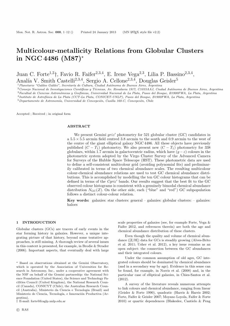
Figure 1. The GMOS field (cyan lines square; 5.5 arcmin on aside) discussed in this work. NGC4486 appears up and to the left.

North is up and East to the left.

Table 1. Observing log of Gemini-GMOS observations.

Date Filter Exposure Airmass Seeing

(sec.) (arcsec)

2010/01/16 g′ 5× 400 1.009 0.632010/01/16-17 r′ 5× 300 1.017 0.602010/01/17 i′ 5× 300 1.147 0.54

2010/01/17 z′ 6× 450 1.080 0.47

spectroscopy of a sample of selected objects that are con-sidered as good GCs candidates (GN-2010A-Q-21; PI: J. C.Forte). The field (5.5 arcmin on a side), centred 3.8 arcmin tothe South and 0.9 arcmin to the West of NGC4486, is shownin Figure 1. The observing log, including dates, filters, ex-posures, mean air mass and composite seeing (FWHM) isgiven in Table 1.

Image processing was performed with the tasks of thepackage gmos within iraf

1. In turn, PSF magnitudes wereobtained with the package daophot within iraf. Theseinstrumental magnitudes were corrected for atmosphericextinction adopting the coefficients given in the Geminiweb pages2, and transformed to the griz′ system usingzero points derived from observations of a standard field(PG123+086), in a way similar to that extensively describedin Faifer et al. (2011). The identification of GC candidates,using both daophot and SExtractor (Bertin & Arnouts1996), also follows the lines described in that paper. The

1 iraf is distributed by the National Optical Astronomy Obser-vatories, which are operated by the Association of Universities for

Research in Astronomy, Inc., under cooperative agreement with

the National Science Foundation.2 http://www.gemini.edu/sciops/instruments/gmos/calibration?q=node/10445

c© RAS, MNRAS 000, 1–12

Multicolour-Metallicity Relations from Globular Clusters in NGC4486 3

Table 2. Cgriz′ photometry errors, in magnitudes.

g′ σg′ σr′ σi′ σz′ σC

20.5 0.011 0.010 0.012 0.019 0.03421.5 0.012 0.010 0.012 0.020 0.03322.5 0.015 0.011 0.014 0.020 0.04523.5 0.027 0.017 0.022 0.035 0.05524.0 0.032 0.021 0.027 0.039 0.070

limiting magnitude of the photometric sample is g′0 ≈ 23.7mag, i.e., ≈ 0.15 mag brighter than the turn-over of theGCs integrated luminosity function (Villegas et al. 2010).The photometric errors, as a function of the g′ magnitudesare given in Table 2.

In what follows we adopt a colour excess E(B − V ) =0.02 mag from the maps by Schlegel, Finkbeiner & Davis(1998), and the interstellar extinction relations given inJordan et al. (2004). The magnitudes and colours, correctedfor interstellar reddening (denoted with the “0” subscript)of our GC sample are given in Table 3.

The 521 GC candidates listed in Table 3 also have(C − T1) photometry obtained with the CTIO Blanco 4-mTelescope and presented in FFG07. The GCs identificationnumbers are from that work. Due to severe incompletenesseffects, data for GCs closer to the galaxy centre were notpublished in FFG07. Among these objects we identified 338that were also observed in the ACS (g−z) colour (Jordan etal. 2009). The photometric values for these GC candidatesare listed in Table 4 where the R.A. and Dec values comefrom this last work.

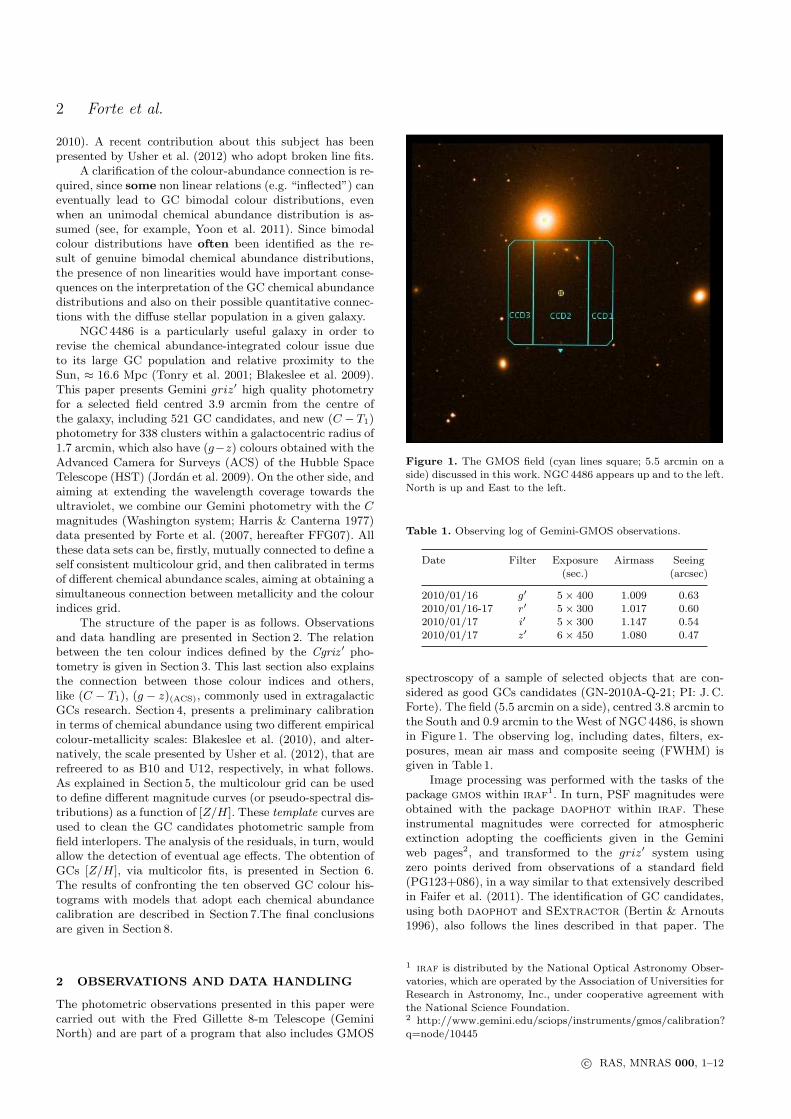
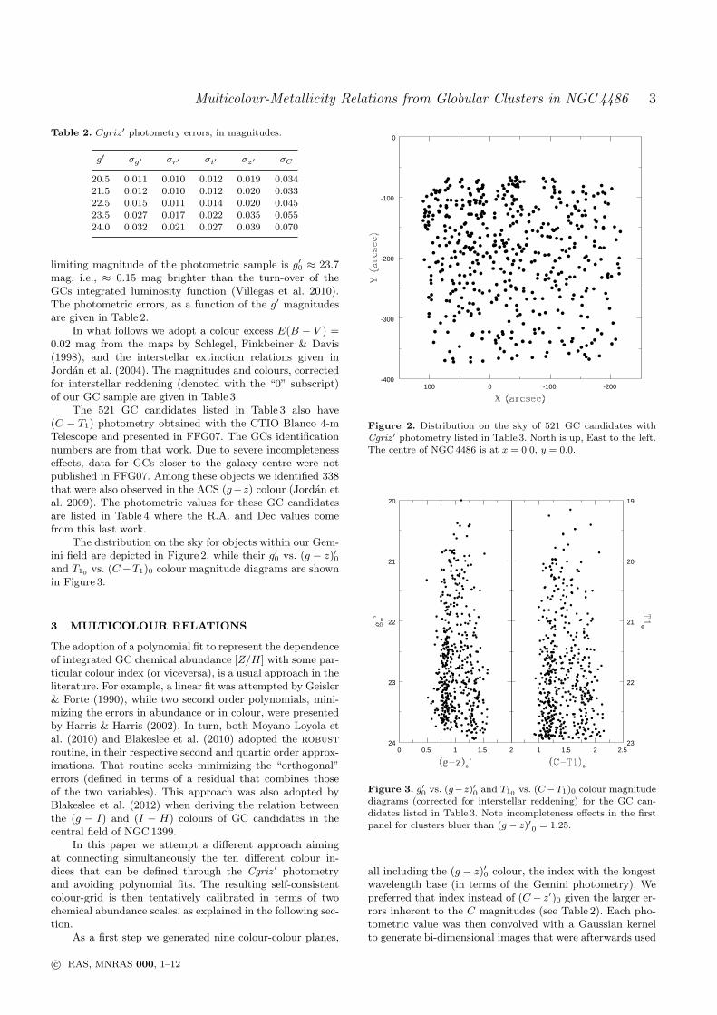
The distribution on the sky for objects within our Gem-ini field are depicted in Figure 2, while their g′0 vs. (g − z)′0and T10 vs. (C−T1)0 colour magnitude diagrams are shownin Figure 3.

3 MULTICOLOUR RELATIONS

The adoption of a polynomial fit to represent the dependenceof integrated GC chemical abundance [Z/H] with some par-ticular colour index (or viceversa), is a usual approach in theliterature. For example, a linear fit was attempted by Geisler& Forte (1990), while two second order polynomials, mini-mizing the errors in abundance or in colour, were presentedby Harris & Harris (2002). In turn, both Moyano Loyola etal. (2010) and Blakeslee et al. (2010) adopted the robust

routine, in their respective second and quartic order approx-imations. That routine seeks minimizing the “orthogonal”errors (defined in terms of a residual that combines thoseof the two variables). This approach was also adopted byBlakeslee et al. (2012) when deriving the relation betweenthe (g − I) and (I − H) colours of GC candidates in thecentral field of NGC1399.

In this paper we attempt a different approach aimingat connecting simultaneously the ten different colour in-dices that can be defined through the Cgriz ′ photometryand avoiding polynomial fits. The resulting self-consistentcolour-grid is then tentatively calibrated in terms of twochemical abundance scales, as explained in the following sec-tion.

As a first step we generated nine colour-colour planes,

100 0 -100 -200-400

-300

-200

-100

0

Figure 2. Distribution on the sky of 521 GC candidates withCgriz ′ photometry listed in Table 3. North is up, East to the left.The centre of NGC4486 is at x = 0.0, y = 0.0.

0 0.5 1 1.5 224

23

22

21

20

1 1.5 2 2.523

22

21

20

19

Figure 3. g′0 vs. (g−z)′0 and T10 vs. (C−T1)0 colour magnitudediagrams (corrected for interstellar reddening) for the GC can-didates listed in Table 3. Note incompleteness effects in the firstpanel for clusters bluer than (g − z)′0 = 1.25.

all including the (g − z)′0 colour, the index with the longestwavelength base (in terms of the Gemini photometry). Wepreferred that index instead of (C− z′)0 given the larger er-rors inherent to the C magnitudes (see Table 2). Each pho-tometric value was then convolved with a Gaussian kernelto generate bi-dimensional images that were afterwards used

c© RAS, MNRAS 000, 1–12

4 Forte et al.

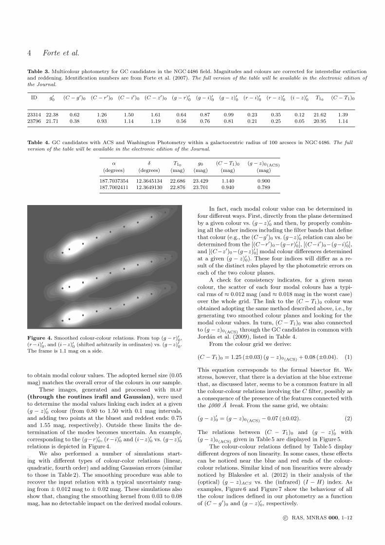
Table 3. Multicolour photometry for GC candidates in the NGC4486 field. Magnitudes and colours are corrected for interstellar extinctionand reddening. Identification numbers are from Forte et al. (2007). The full version of the table will be available in the electronic edition ofthe Journal.

ID g′0 (C − g′)0 (C − r′)0 (C − i′)0 (C − z′)0 (g − r)′0 (g − i)′0 (g − z)′0 (r − i)′0 (r − z)′0 (i− z)′0 T10 (C − T1)0

23314 22.38 0.62 1.26 1.50 1.61 0.64 0.87 0.99 0.23 0.35 0.12 21.62 1.3923796 21.71 0.38 0.93 1.14 1.19 0.56 0.76 0.81 0.21 0.25 0.05 20.95 1.14

Table 4. GC candidates with ACS and Washington Photometry within a galactocentric radius of 100 arcsecs in NGC4486. The full

version of the table will be available in the electronic edition of the Journal.

α δ T10 g0 (C − T1)0 (g − z)0(ACS)

(degrees) (degrees) (mag) (mag) (mag) (mag)

187.7037354 12.3645134 22.686 23.429 1.140 0.900187.7002411 12.3649130 22.876 23.701 0.940 0.789

Figure 4. Smoothed colour-colour relations. From top (g − r)′0,

(r− i)′0, and (i−z)′0 (shifted arbitrarily in ordinates) vs. (g−z)′0.The frame is 1.1 mag on a side.

to obtain modal colour values. The adopted kernel size (0.05mag) matches the overall error of the colours in our sample.

These images, generated and processed with iraf

(through the routines irafil and Gaussian), were usedto determine the modal values linking each index at a given(g − z)′0 colour (from 0.80 to 1.50 with 0.1 mag intervals,and adding two points at the bluest and reddest ends: 0.75and 1.55 mag, respectively). Outside these limits the de-termination of the modes becomes uncertain. An example,corresponding to the (g−r)′0, (r−i)′0 and (i−z)′0 vs. (g−z)′0relations is depicted in Figure 4.

We also performed a number of simulations start-ing with different types of colour-color relations (linear,quadratic, fourth order) and adding Gaussian errors (similarto those in Table 2). The smoothing procedure was able torecover the input relation with a typical uncertainty rang-ing from ± 0.012 mag to ± 0.02 mag. These simulations alsoshow that, changing the smoothing kernel from 0.03 to 0.08mag, has no detectable impact on the derived modal colours.

In fact, each modal colour value can be determined infour different ways. First, directly from the plane determinedby a given colour vs. (g−z)′0 and then, by properly combin-ing all the other indices including the filter bands that definethat colour (e.g., the (C−g′)0 vs. (g−z)′0 relation can also bedetermined from the [(C−r′)0−(g−r)′0], [(C−i′)0−(g−i)′0],and [(C−z′)0−(g−z)′0] modal colour differences determinedat a given (g − z)′0). These four indices will differ as a re-sult of the distinct roles played by the photometric errors oneach of the two colour planes.

A check for consistency indicates, for a given meancolour, the scatter of each four modal colours has a typi-cal rms of ≈ 0.012 mag (and ≈ 0.018 mag in the worst case)over the whole grid. The link to the (C − T1)0 colour wasobtained adopting the same method described above, i.e., bygenerating two smoothed colour planes and looking for themodal colour values. In turn, (C − T1)0 was also connectedto (g − z)0(ACS) through the GC candidates in common withJordan et al. (2009), listed in Table 4.

From the colour grid we derive:

(C − T1)0 = 1.25 (±0.03) (g − z)0(ACS) + 0.08 (±0.04). (1)

This equation corresponds to the formal bisector fit. Westress, however, that there is a deviation at the blue extremethat, as discussed later, seems to be a common feature in allthe colour-colour relations involving the C filter, possibly asa consequence of the presence of the features connected withthe 4000 A break. From the same grid, we obtain:

(g − z)′0 = (g − z)0(ACS) − 0.07 (±0.02). (2)

The relations between (C − T1)0 and (g − z)′0 with(g − z)0(ACS) given in Table 5 are displayed in Figure 5.

The colour-colour relations defined by Table 5 displaydifferent degrees of non linearity. In some cases, these effectscan be noticed near the blue and red ends of the colour-colour relations. Similar kind of non linearities were alreadynoticed by Blakeslee et al. (2012) in their analysis of the(optical) (g − z)ACS vs. the (infrared) (I − H) index. Asexamples, Figure 6 and Figure 7 show the behaviour of allthe colour indices defined in our photometry as a functionof (C − g′)0 and (g − z)′0, respectively.

c© RAS, MNRAS 000, 1–12

Multicolour-Metallicity Relations from Globular Clusters in NGC4486 5

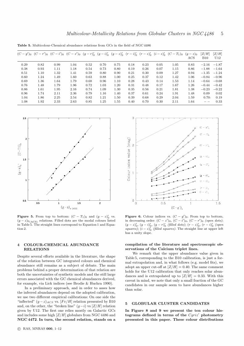
Table 5. Multicolour-Chemical abundance relations from GCs in the field of NGC4486

(C − g′)0 (C − r′)0 (C − i′)0 (C − z′)0 (g − r)′0 (g − i)′0 (g − z)′0 (r − i)′0 (r − z)′0 (i− z)′0 (C − T1)0 (g − z)0 [Z/H] [Z/H]ACS B10 U12

0.29 0.82 0.99 1.04 0.52 0.70 0.75 0.18 0.23 0.05 1.05 0.83 −2.16 −1.870.38 0.93 1.11 1.18 0.54 0.73 0.80 0.19 0.26 0.07 1.15 0.86 −1.88 −1.64

0.51 1.10 1.32 1.41 0.59 0.80 0.90 0.21 0.30 0.09 1.27 0.94 −1.35 −1.240.60 1.24 1.49 1.60 0.63 0.88 1.00 0.25 0.37 0.12 1.42 1.06 −0.84 −0.960.69 1.36 1.64 1.79 0.68 0.96 1.10 0.28 0.43 0.14 1.53 1.14 −0.64 −0.680.76 1.48 1.79 1.96 0.72 1.03 1.20 0.31 0.48 0.17 1.67 1.26 −0.44 −0.42

0.86 1.61 1.95 2.16 0.74 1.09 1.30 0.35 0.56 0.21 1.81 1.38 −0.23 −0.220.96 1.74 2.11 2.36 0.79 1.16 1.40 0.37 0.61 0.24 1.91 1.48 0.09 0.021.04 1.86 2.25 2.54 0.82 1.21 1.50 0.39 0.68 0.29 2.04 1.59 0.70: 0.19

1.08 1.92 2.33 2.63 0.85 1.25 1.55 0.40 0.70 0.30 2.11 1.64 −− 0.33

0.5 1 1.5 20.5

1

1.5

2

2.5

0.5 1 1.5 20.5

1

1.5

2

2.5

Figure 5. From top to bottom: (C − T1)0 and (g − z)′0 vs.(g − z)0(ACS) relations. Filled dots are the modal colours listedin Table 5. The straight lines correspond to Equation 1 and Equa-tion 2.

4 COLOUR-CHEMICAL ABUNDANCERELATIONS

Despite several efforts available in the literature, the shapeof the relation between GC integrated colours and chemicalabundance still remains as a subject of debate. The mainproblems behind a proper determination of that relation areboth the uncertainties of synthetic models and the still largeerrors associated with the GC chemical abundances derived,for example, via Lick indices (see Brodie & Huchra 1990).

In a preliminary approach, and in order to asses howthe inferred abundances depend on the adopted calibration,we use two different empirical calibrations: On one side the“inflected” (g−z)ACS vs. [Fe/H] relation presented by B10and, on the other, the “broken line” (g−i) vs [Z/H] relationgiven by U12. The first one relies mostly on Galactic GCsand includes some high [Z/H] globulars from NGC4486 andNGC4472. In turn, the second relation, stands on a

Figure 6. Colour indices vs. (C − g′)0. From top to bottom,in decreasing order: (C − z′)0, (C − i′)0, (C − r′)0 (open dots);(g − z)′0, (g − i)′0, (g − r)′0 (filled dots); (r − z)′0, (r − i)′0 (opensquares); (i− z)′0 (filled squares). The straight line at upper left

has a unity slope.

compilation of the literature and spectroscopic ob-servations of the Calcium triplet lines.

We remark that the upper abundance value given inTable 5, corresponding to the B10 calibration, is just a for-mal extrapolation and, in what follows (e.g. model fits), weadopt an upper cut-off at [Z/H] = 0.40. The same commentholds for the U12 calibration that only reaches solar abun-dances and is extrapolated up to [Z/H] = 0.33. With thiscaveat in mind, we note that only a small fraction of the GCcandidates in our sample seem to have abundances higherthan solar.

5 GLOBULAR CLUSTER CANDIDATES

In Figure 8 and 9 we present the ten colour his-tograms defined in terms of the Cgriz′ photometrypresented in this paper. These colour distributions

c© RAS, MNRAS 000, 1–12

6 Forte et al.

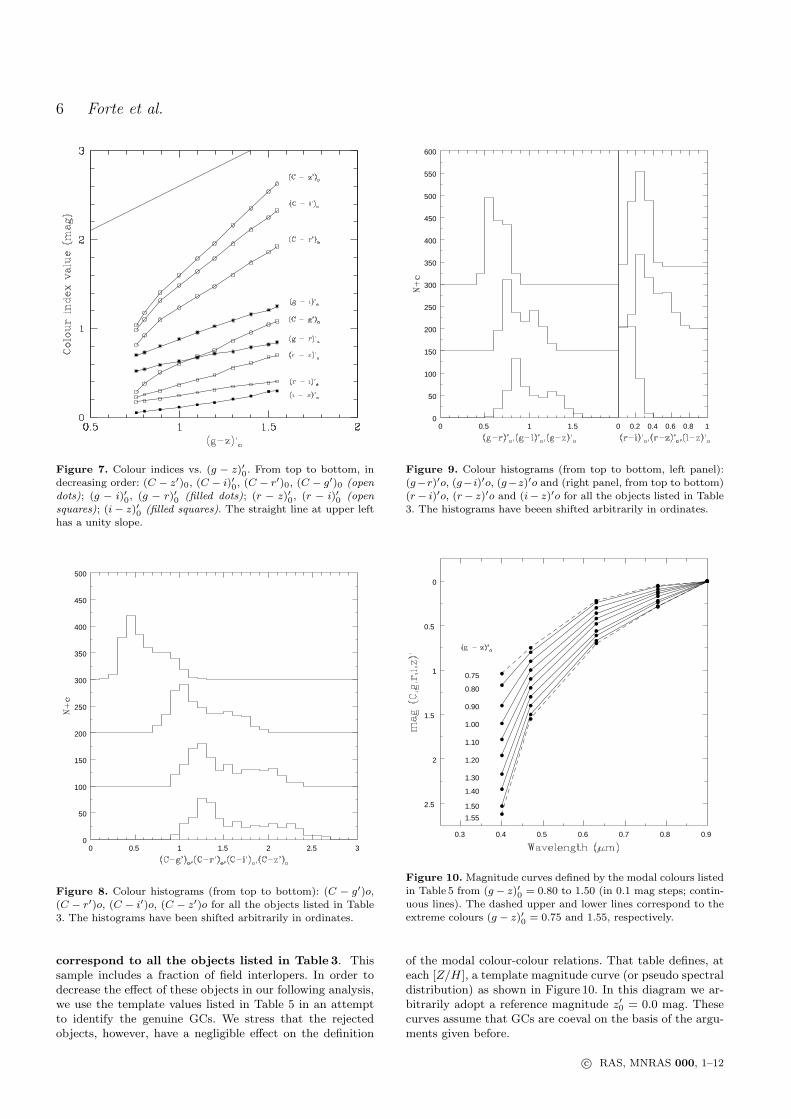
Figure 7. Colour indices vs. (g − z)′0. From top to bottom, indecreasing order: (C − z′)0, (C − i)′0, (C − r′)0, (C − g′)0 (opendots); (g − i)′0, (g − r)′0 (filled dots); (r − z)′0, (r − i)′0 (open

squares); (i− z)′0 (filled squares). The straight line at upper lefthas a unity slope.

0 0.5 1 1.5 2 2.5 30

50

100

150

200

250

300

350

400

450

500

Figure 8. Colour histograms (from top to bottom): (C − g′)o,(C − r′)o, (C − i′)o, (C − z′)o for all the objects listed in Table

3. The histograms have been shifted arbitrarily in ordinates.

correspond to all the objects listed in Table 3. Thissample includes a fraction of field interlopers. In order todecrease the effect of these objects in our following analysis,we use the template values listed in Table 5 in an attemptto identify the genuine GCs. We stress that the rejectedobjects, however, have a negligible effect on the definition

0 0.5 1 1.50

50

100

150

200

250

300

350

400

450

500

550

600

0 0.2 0.4 0.6 0.8 1

Figure 9. Colour histograms (from top to bottom, left panel):(g−r)′o, (g− i)′o, (g−z)′o and (right panel, from top to bottom)(r− i)′o, (r− z)′o and (i− z)′o for all the objects listed in Table

3. The histograms have beeen shifted arbitrarily in ordinates.

0.3 0.4 0.5 0.6 0.7 0.8 0.9

2.5

2

1.5

1

0.5

0

0.75

0.80

0.90

1.00

1.10

1.20

1.30

1.40

1.50

1.55

Figure 10. Magnitude curves defined by the modal colours listedin Table 5 from (g − z)′0 = 0.80 to 1.50 (in 0.1 mag steps; contin-uous lines). The dashed upper and lower lines correspond to theextreme colours (g − z)′0 = 0.75 and 1.55, respectively.

of the modal colour-colour relations. That table defines, ateach [Z/H], a template magnitude curve (or pseudo spectraldistribution) as shown in Figure 10. In this diagram we ar-bitrarily adopt a reference magnitude z′0 = 0.0 mag. Thesecurves assume that GCs are coeval on the basis of the argu-ments given before.

c© RAS, MNRAS 000, 1–12

Multicolour-Metallicity Relations from Globular Clusters in NGC4486 7

19 20 21 22 230

0.05

0.1

0.15

0.2

i’o

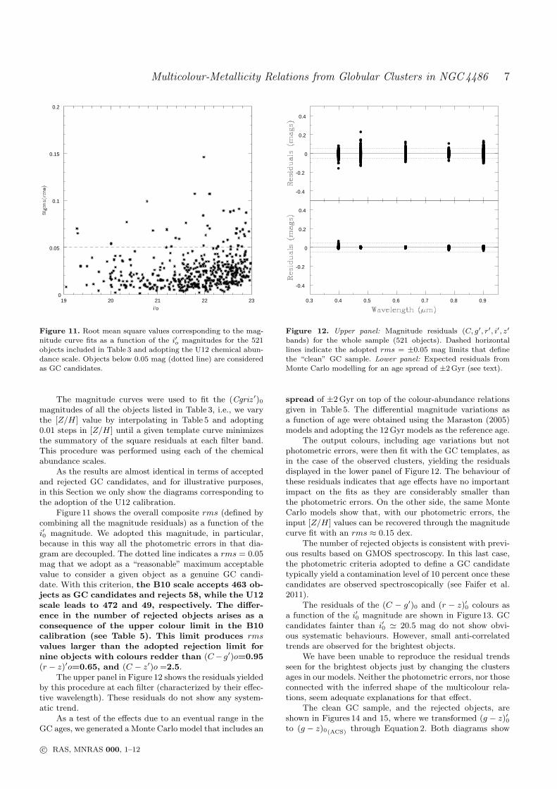
Figure 11. Root mean square values corresponding to the mag-nitude curve fits as a function of the i′o magnitudes for the 521objects included in Table 3 and adopting the U12 chemical abun-

dance scale. Objects below 0.05 mag (dotted line) are considered

as GC candidates.

The magnitude curves were used to fit the (Cgriz ′)0magnitudes of all the objects listed in Table 3, i.e., we varythe [Z/H] value by interpolating in Table 5 and adopting0.01 steps in [Z/H] until a given template curve minimizesthe summatory of the square residuals at each filter band.This procedure was performed using each of the chemicalabundance scales.

As the results are almost identical in terms of acceptedand rejected GC candidates, and for illustrative purposes,in this Section we only show the diagrams corresponding tothe adoption of the U12 calibration.

Figure 11 shows the overall composite rms (defined bycombining all the magnitude residuals) as a function of thei′0 magnitude. We adopted this magnitude, in particular,because in this way all the photometric errors in that dia-gram are decoupled. The dotted line indicates a rms = 0.05mag that we adopt as a “reasonable” maximum acceptablevalue to consider a given object as a genuine GC candi-date. With this criterion, the B10 scale accepts 463 ob-jects as GC candidates and rejects 58, while the U12scale leads to 472 and 49, respectively. The differ-ence in the number of rejected objects arises as aconsequence of the upper colour limit in the B10calibration (see Table 5). This limit produces rmsvalues larger than the adopted rejection limit fornine objects with colours redder than (C−g′)o=0.95(r − z)′o=0.65, and (C − z′)o =2.5.

The upper panel in Figure 12 shows the residuals yieldedby this procedure at each filter (characterized by their effec-tive wavelength). These residuals do not show any system-atic trend.

As a test of the effects due to an eventual range in theGC ages, we generated a Monte Carlo model that includes an

-0.4

-0.2

0

0.2

0.4

0.3 0.4 0.5 0.6 0.7 0.8 0.9

-0.4

-0.2

0

0.2

0.4

Figure 12. Upper panel: Magnitude residuals (C, g′, r′, i′, z′

bands) for the whole sample (521 objects). Dashed horizontallines indicate the adopted rms = ±0.05 mag limits that define

the “clean” GC sample. Lower panel: Expected residuals fromMonte Carlo modelling for an age spread of ±2Gyr (see text).

spread of ±2Gyr on top of the colour-abundance relationsgiven in Table 5. The differential magnitude variations asa function of age were obtained using the Maraston (2005)models and adopting the 12Gyr models as the reference age.

The output colours, including age variations but notphotometric errors, were then fit with the GC templates, asin the case of the observed clusters, yielding the residualsdisplayed in the lower panel of Figure 12. The behaviour ofthese residuals indicates that age effects have no importantimpact on the fits as they are considerably smaller thanthe photometric errors. On the other side, the same MonteCarlo models show that, with our photometric errors, theinput [Z/H] values can be recovered through the magnitudecurve fit with an rms ≈ 0.15 dex.

The number of rejected objects is consistent with previ-ous results based on GMOS spectroscopy. In this last case,the photometric criteria adopted to define a GC candidatetypically yield a contamination level of 10 percent once thesecandidates are observed spectroscopically (see Faifer et al.2011).

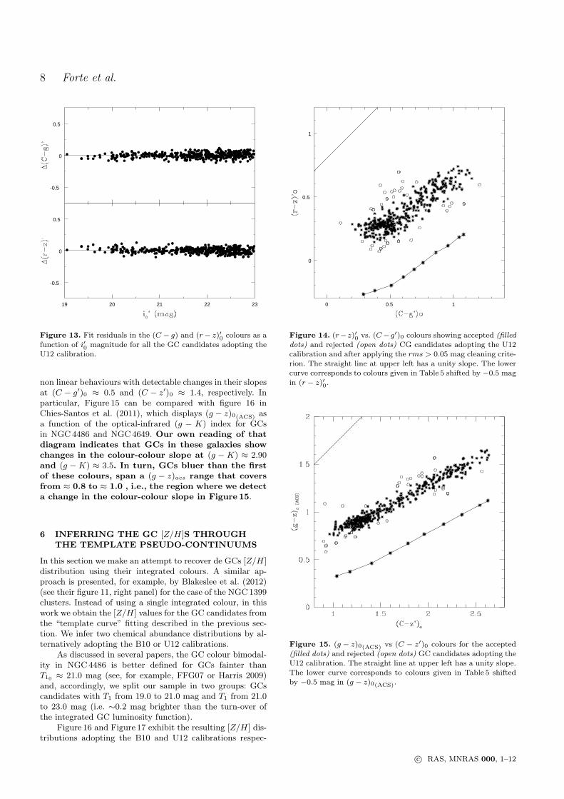
The residuals of the (C − g′)0 and (r − z)′0 colours asa function of the i′0 magnitude are shown in Figure 13. GCcandidates fainter than i′0 ≃ 20.5 mag do not show obvi-ous systematic behaviours. However, small anti-correlatedtrends are observed for the brightest objects.

We have been unable to reproduce the residual trendsseen for the brightest objects just by changing the clustersages in our models. Neither the photometric errors, nor thoseconnected with the inferred shape of the multicolour rela-tions, seem adequate explanations for that effect.

The clean GC sample, and the rejected objects, areshown in Figures 14 and 15, where we transformed (g − z)′0to (g − z)0(ACS) through Equation 2. Both diagrams show

c© RAS, MNRAS 000, 1–12

8 Forte et al.

-0.5

0

0.5

19 20 21 22 23

-0.5

0

0.5

Figure 13. Fit residuals in the (C − g) and (r− z)′0 colours as afunction of i′0 magnitude for all the GC candidates adopting theU12 calibration.

non linear behaviours with detectable changes in their slopesat (C − g′)0 ≈ 0.5 and (C − z′)0 ≈ 1.4, respectively. Inparticular, Figure 15 can be compared with figure 16 inChies-Santos et al. (2011), which displays (g − z)0(ACS) asa function of the optical-infrared (g − K) index for GCsin NGC4486 and NGC4649. Our own reading of thatdiagram indicates that GCs in these galaxies showchanges in the colour-colour slope at (g − K) ≈ 2.90and (g −K) ≈ 3.5. In turn, GCs bluer than the firstof these colours, span a (g − z)acs range that coversfrom ≈ 0.8 to ≈ 1.0 , i.e., the region where we detecta change in the colour-colour slope in Figure 15.

6 INFERRING THE GC [Z/H]S THROUGHTHE TEMPLATE PSEUDO-CONTINUUMS

In this section we make an attempt to recover de GCs [Z/H]distribution using their integrated colours. A similar ap-proach is presented, for example, by Blakeslee et al. (2012)(see their figure 11, right panel) for the case of the NGC1399clusters. Instead of using a single integrated colour, in thiswork we obtain the [Z/H] values for the GC candidates fromthe “template curve” fitting described in the previous sec-tion. We infer two chemical abundance distributions by al-ternatively adopting the B10 or U12 calibrations.

As discussed in several papers, the GC colour bimodal-ity in NGC4486 is better defined for GCs fainter thanT10 ≈ 21.0 mag (see, for example, FFG07 or Harris 2009)and, accordingly, we split our sample in two groups: GCscandidates with T1 from 19.0 to 21.0 mag and T1 from 21.0to 23.0 mag (i.e. ∼0.2 mag brighter than the turn-over ofthe integrated GC luminosity function).

Figure 16 and Figure 17 exhibit the resulting [Z/H] dis-tributions adopting the B10 and U12 calibrations respec-

0 0.5 1

0

0.5

1

Figure 14. (r−z)′0 vs. (C−g′)0 colours showing accepted (filleddots) and rejected (open dots) CG candidates adopting the U12calibration and after applying the rms > 0.05 mag cleaning crite-

rion. The straight line at upper left has a unity slope. The lowercurve corresponds to colours given in Table 5 shifted by −0.5 magin (r − z)′0.

Figure 15. (g − z)0(ACS) vs (C − z′)0 colours for the accepted(filled dots) and rejected (open dots) GC candidates adopting theU12 calibration. The straight line at upper left has a unity slope.The lower curve corresponds to colours given in Table 5 shiftedby −0.5 mag in (g − z)0(ACS).

c© RAS, MNRAS 000, 1–12

Multicolour-Metallicity Relations from Globular Clusters in NGC4486 9

tively and for the two GC groups. In both diagrams thebrightest clusters show distinct behaviours when comparedwith the fainter counterparts. For those GCs the abundancedistributions seem broad and unimodal.

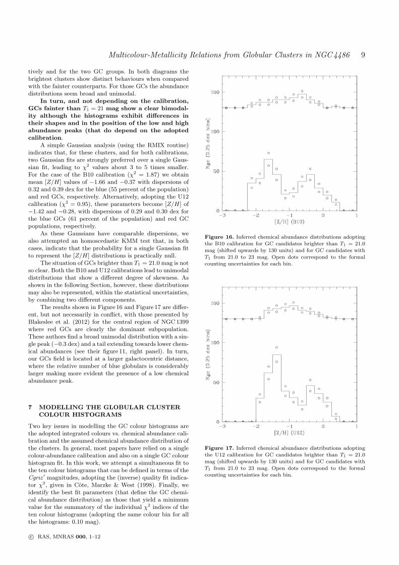
In turn, and not depending on the calibration,GCs fainter than T1 = 21 mag show a clear bimodal-ity although the histograms exhibit differences intheir shapes and in the position of the low and highabundance peaks (that do depend on the adoptedcalibration.

A simple Gaussian analysis (using the RMIX routine)indicates that, for these clusters, and for both calibrations,two Gaussian fits are strongly preferred over a single Gaus-sian fit, leading to χ2 values about 3 to 5 times smaller.For the case of the B10 calibration (χ2 = 1.87) we obtainmean [Z/H] values of −1.66 and −0.37 with dispersions of0.32 and 0.39 dex for the blue (55 percent of the population)and red GCs, respectively. Alternatively, adopting the U12calibration (χ2 = 0.95), these parameters become [Z/H] of−1.42 and −0.28, with dispersions of 0.29 and 0.30 dex forthe blue GCs (61 percent of the population) and red GCpopulations, respectively.

As these Gaussians have comparable dispersions, wealso attempted an homoscedastic KMM test that, in bothcases, indicate that the probability for a single Gaussian fitto represent the [Z/H] distributions is practically null.

The situation of GCs brighter than T1 = 21.0 mag is notso clear. Both the B10 and U12 calibrations lead to unimodaldistributions that show a different degree of skewness. Asshown in the following Section, however, these distributionsmay also be represented, within the statistical uncertainties,by combining two different components.

The results shown in Figure 16 and Figure 17 are differ-ent, but not necessarily in conflict, with those presented byBlakeslee et al. (2012) for the central region of NGC1399where red GCs are clearly the dominant subpopulation.These authors find a broad unimodal distribution with a sin-gle peak (−0.3 dex) and a tail extending towards lower chem-ical abundances (see their figure 11, right panel). In turn,our GCs field is located at a larger galactocentric distance,where the relative number of blue globulars is considerablylarger making more evident the presence of a low chemicalabundance peak.

7 MODELLING THE GLOBULAR CLUSTERCOLOUR HISTOGRAMS

Two key issues in modelling the GC colour histograms arethe adopted integrated colours vs. chemical abundance cali-bration and the assumed chemical abundance distribution ofthe clusters. In general, most papers have relied on a singlecolour-abundance calibration and also on a single GC colourhistogram fit. In this work, we attempt a simultaneous fit tothe ten colour histograms that can be defined in terms of theCgriz ′ magnitudes, adopting the (inverse) quality fit indica-tor χ2, given in Cote, Marzke & West (1998). Finally, weidentify the best fit parameters (that define the GC chemi-cal abundance distribution) as those that yield a minimumvalue for the summatory of the individual χ2 indices of theten colour histograms (adopting the same colour bin for allthe histograms: 0.10 mag).

Figure 16. Inferred chemical abundance distributions adoptingthe B10 calibration for GC candidates brighter than T1 = 21.0mag (shifted upwards by 130 units) and for GC candidates with

T1 from 21.0 to 23 mag. Open dots correspond to the formalcounting uncertainties for each bin.

Figure 17. Inferred chemical abundance distributions adoptingthe U12 calibration for GC candidates brighter than T1 = 21.0

mag (shifted upwards by 130 units) and for GC candidates withT1 from 21.0 to 23 mag. Open dots correspond to the formalcounting uncertainties for each bin.

c© RAS, MNRAS 000, 1–12

10 Forte et al.

Monte Carlo model histograms were obtained followingthe same procedure explained in Forte et al. (2012). First,we generate “seed” globulars with chemical abundances Z(within the range Zi to Zmax) whose numbers are controlledby a given distribution function NGC(Z).

After trying different simple distributions, we concludedas in FFG07, that a double exponential dependence:

NGC(Z) ≈ exp(−Z/Zs) (3)

(where Zs is the scale lenght corresponding to the blueor red GC subpopulation) is the simplest function that al-lows a fit to the colour histograms based on a minimum

number of free parameters. Formally, this approach requiresseven parameters: the ratio of blue to red clusters, and foreach GC subpopulation the Zi and Zmax values as well as thechemical scale lenght Zs. In fact, the free parameters werereduced to five, as the minimum chemical abundance of theblue GCs subpopulation, as well as the maximum chemicalabundance of the red GCs, were set as the lowest and uppervalues in the B10 and U12 calibrations.

The integrated colours for each GC were obtained bylinear interpolation, using the logarithmic abundance as ar-gument, in Table 5.

For each synthetic cluster we also generate an apparentmagnitude g′0, adopting a Gaussian integrated luminosityfunction and according to the parameters given by Ville-gas et al. (2010). These magnitudes were used as input inTable 2 in order to model (also Gaussian) observing errorsthat were added to each colour. Given the relatively shortrange in apparent magnitude, we do not include an explicitdependence of chemical abundance with brightness for theblue globulars (i.e., the “blue tilt” effect; see, for example,Harris 2009).

The parameters that define the chemical abundance dis-tributions and provide the best overall fit to the ten colourhistograms in each case, are listed in Table 6, and the corre-sponding individual and cumulative χ2 indices are given inTable 7 and Table 8.

Even though both models lead to N(GC) values within≈ 1.5 times the formal counting errors of each histogram bin,the U12 calibration yields better fits in terms of the cumu-lative quality index. We remark that this statement is validonly if the bi-exponential parametrization of the chemicalabundance is accepted.

Each of the parameters listed in Table 6 has an associ-ated uncertainty which we define as the parameter variationthat leads to a decrease of the fit quality, indicated by anincrease of ten percent above the mimimum total χ2 valuein the five free parameters space.

Following this, we get typical uncertainties of ± 10 GCsfor each subpopulation; for the blue GCs: ± 0.01 Z⊙ in ZsB

and ± 0.05 Z⊙ in Zmax; and for the red GCs: ± 0.06 Z⊙ inZsR and ± 0.02 Z⊙ in Zi.

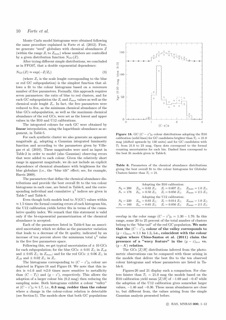
The histograms corresponding to (C − z′)0 colour aredepicted in Figure 18 and Figure 19. We note that this in-dex is ≈1.6 and ≈2.0 times more sensitive to metallicitythan (C − T1) and (g − z′), respectively. This allows theadoption of a larger colour bin (0.2 mag) then reducing thesampling noise. Both histograms exhibit a colour “valley”at (C− z′)0 ≈ 1.7, i.e., 0.3 mag. redder than the colourwhere a change in the colour-colour relation is detectable(see Section 5). The models show that both GC populations

Figure 18. GC (C − z′)0 colour distributions adopting the B10calibration (solid lines) for GC candidates brighter than T1 = 21.0mag (shifted upwards by 130 units) and for GC candidates with

T1 from 21.0 to 23 mag. Open dots correspond to the formalcounting uncertainties for each bin. Dashed lines correspond to

the best fit models given in Table 6.

Table 6. Parameters of the chemical abundance distributions

giving the best overall fit to the colour histograms for GlobularClusters fainter than T1 = 21.

Adopting the B10 calibration:Nb = 200 Zsb = 0.02 Z⊙ Zi = 0.007 Z⊙ Zmax = 1.0 Z⊙

Nr = 178 Zsr = 0.50 Z⊙ Zi = 0.050 Z⊙ Zmax = 2.5 Z⊙

Adopting the U12 calibration:Nb = 220 Zsb = 0.03 Z⊙ Zi = 0.014 Z⊙ Zmax = 1.0 Z⊙

Nr = 160 Zsr = 0.65 Z⊙ Zi = 0.050 Z⊙ Zmax = 2.5 Z⊙

overlap in the color range (C − z′)0 = 1.30 − 1.70. In thisrange, some 20 to 25 percent of the total number of clustersbelong to the “blue tail” of the red GC population.We notethat the (C− z′)0 colour of the valley corresponds to(g− z)0acs ≈ 1.1 to 1.2, i.e., coincident with the colourregion where Chies-Santos et al. (2011) claim thepresence of a ”wavy feature” in the (g − z)acs vs.(g −K) relation.

The GCs [Z/H] distributions inferred from the photo-metric observations can be compared with those arising inthe models that deliver the best fits to the ten observedcolour histograms and whose parameters are listed in Ta-ble 6.

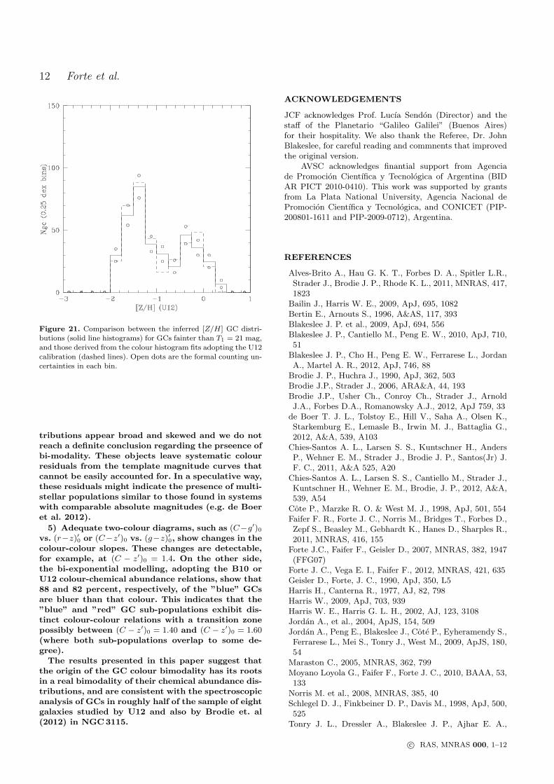
Figures 20 and 21 display such a comparison. For clus-ters fainter than T1 = 21.0 mag the models based on theB10 calibration yield mean [Z/H] of −1.69 and −0.47 whilethe adoption of the U12 calibration gives somewhat largervalues, −1.46 and −0.36. These mean abundances are closeto, but different from, the values arising from the simpleGaussian analysis presented before.

c© RAS, MNRAS 000, 1–12

Multicolour-Metallicity Relations from Globular Clusters in NGC4486 11

Table 7. GC Colour histograms fit χ2 adopting the B10 calibration. First line, GCs brighter than T1 = 21.0 mag; second line: GCs fainterthan T1 = 21.0 mag.

(C − g)′0 (C − r)0′ (C − i)0′ (C − z)0′ (g − r)′0 (g − i)0′ (g − z)′0 (r − i)′0 (r − z)′0 (i− z)′0 Cumulative χ2

0.85 0.64 0.90 0.74 0.61 0.92 0.41 0.08 1.41 1.42 7.980.56 1.18 1.07 1.13 0.84 1.29 1.62 0.41 1.76 1.60 11.46

Table 8. GC Colour histograms fit χ2 adopting the U12 calibration. First line, GCs brighter than T1 = 21.0 mag; second line: GCs fainterthan T1 = 21.0 mag.

(C − g)′0 (C − r)0′ (C − i)0′ (C − z)0′ (g − r)′0 (g − i)0′ (g − z)′0 (r − i)′0 (r − z)′0 (i− z)′0 Cumulative χ2

0.62 0.56 0.61 0.59 0.62 0.59 0.49 0.11 0.58 0.37 5.270.62 0.90 0.61 0.80 1.15 0.56 0.95 0.44 0.77 0.62 7.42

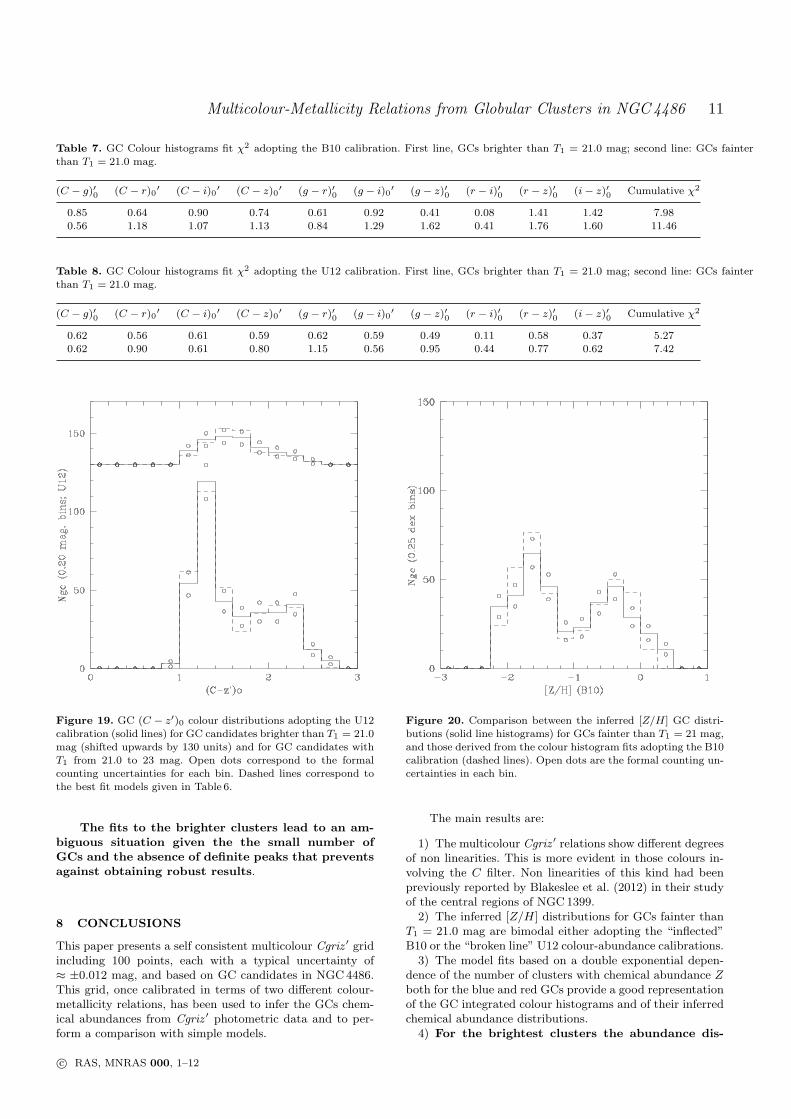
Figure 19. GC (C − z′)0 colour distributions adopting the U12calibration (solid lines) for GC candidates brighter than T1 = 21.0mag (shifted upwards by 130 units) and for GC candidates with

T1 from 21.0 to 23 mag. Open dots correspond to the formalcounting uncertainties for each bin. Dashed lines correspond to

the best fit models given in Table 6.

The fits to the brighter clusters lead to an am-biguous situation given the the small number ofGCs and the absence of definite peaks that preventsagainst obtaining robust results.

8 CONCLUSIONS

This paper presents a self consistent multicolour Cgriz ′ gridincluding 100 points, each with a typical uncertainty of≈ ±0.012 mag, and based on GC candidates in NGC4486.This grid, once calibrated in terms of two different colour-metallicity relations, has been used to infer the GCs chem-ical abundances from Cgriz ′ photometric data and to per-form a comparison with simple models.

Figure 20. Comparison between the inferred [Z/H] GC distri-butions (solid line histograms) for GCs fainter than T1 = 21 mag,and those derived from the colour histogram fits adopting the B10

calibration (dashed lines). Open dots are the formal counting un-

certainties in each bin.

The main results are:

1) The multicolour Cgriz ′ relations show different degreesof non linearities. This is more evident in those colours in-volving the C filter. Non linearities of this kind had beenpreviously reported by Blakeslee et al. (2012) in their studyof the central regions of NGC1399.

2) The inferred [Z/H] distributions for GCs fainter thanT1 = 21.0 mag are bimodal either adopting the “inflected”B10 or the “broken line” U12 colour-abundance calibrations.

3) The model fits based on a double exponential depen-dence of the number of clusters with chemical abundance Zboth for the blue and red GCs provide a good representationof the GC integrated colour histograms and of their inferredchemical abundance distributions.

4) For the brightest clusters the abundance dis-

c© RAS, MNRAS 000, 1–12

12 Forte et al.

Figure 21. Comparison between the inferred [Z/H] GC distri-butions (solid line histograms) for GCs fainter than T1 = 21 mag,and those derived from the colour histogram fits adopting the U12

calibration (dashed lines). Open dots are the formal counting un-

certainties in each bin.

tributions appear broad and skewed and we do notreach a definite conclusion regarding the prseence ofbi-modality. These objects leave systematic colourresiduals from the template magnitude curves thatcannot be easily accounted for. In a speculative way,these residuals might indicate the presence of multi-stellar populations similar to those found in systemswith comparable absolute magnitudes (e.g. de Boeret al. 2012).

5) Adequate two-colour diagrams, such as (C−g′)0vs. (r−z)′0 or (C−z′)0 vs. (g−z)′0, show changes in thecolour-colour slopes. These changes are detectable,for example, at (C − z′)0 = 1.4. On the other side,the bi-exponential modelling, adopting the B10 orU12 colour-chemical abundance relations, show that88 and 82 percent, respectively, of the ”blue” GCsare bluer than that colour. This indicates that the”blue” and ”red” GC sub-populations exhibit dis-tinct colour-colour relations with a transition zonepossibly between (C − z′)0 = 1.40 and (C − z′)0 = 1.60(where both sub-populations overlap to some de-gree).

The results presented in this paper suggest thatthe origin of the GC colour bimodality has its rootsin a real bimodality of their chemical abundance dis-tributions, and are consistent with the spectroscopicanalysis of GCs in roughly half of the sample of eightgalaxies studied by U12 and also by Brodie et. al(2012) in NGC3115.

ACKNOWLEDGEMENTS

JCF acknowledges Prof. Lucıa Sendon (Director) and thestaff of the Planetario “Galileo Galilei” (Buenos Aires)for their hospitality. We also thank the Referee, Dr. JohnBlakeslee, for careful reading and commnents that improvedthe original version.

AVSC acknowledges finantial support from Agenciade Promocion Cientıfica y Tecnologica of Argentina (BIDAR PICT 2010-0410). This work was supported by grantsfrom La Plata National University, Agencia Nacional dePromocion Cientıfica y Tecnologica, and CONICET (PIP-200801-1611 and PIP-2009-0712), Argentina.

REFERENCES

Alves-Brito A., Hau G. K. T., Forbes D. A., Spitler L.R.,Strader J., Brodie J. P., Rhode K. L., 2011, MNRAS, 417,1823

Bailin J., Harris W. E., 2009, ApJ, 695, 1082Bertin E., Arnouts S., 1996, A&AS, 117, 393Blakeslee J. P. et al., 2009, ApJ, 694, 556Blakeslee J. P., Cantiello M., Peng E. W., 2010, ApJ, 710,51

Blakeslee J. P., Cho H., Peng E. W., Ferrarese L., JordanA., Martel A. R., 2012, ApJ, 746, 88

Brodie J. P., Huchra J., 1990, ApJ, 362, 503Brodie J.P., Strader J., 2006, ARA&A, 44, 193Brodie J.P., Usher Ch., Conroy Ch., Strader J., ArnoldJ.A., Forbes D.A., Romanowsky A.J., 2012, ApJ 759, 33

de Boer T. J. L., Tolstoy E., Hill V., Saha A., Olsen K.,Starkemburg E., Lemasle B., Irwin M. J., Battaglia G.,2012, A&A, 539, A103

Chies-Santos A. L., Larsen S. S., Kuntschner H., AndersP., Wehner E. M., Strader J., Brodie J. P., Santos(Jr) J.F. C., 2011, A&A 525, A20

Chies-Santos A. L., Larsen S. S., Cantiello M., Strader J.,Kuntschner H., Wehner E. M., Brodie, J. P., 2012, A&A,539, A54

Cote P., Marzke R. O. & West M. J., 1998, ApJ, 501, 554Faifer F. R., Forte J. C., Norris M., Bridges T., Forbes D.,Zepf S., Beasley M., Gebhardt K., Hanes D., Sharples R.,2011, MNRAS, 416, 155

Forte J.C., Faifer F., Geisler D., 2007, MNRAS, 382, 1947(FFG07)

Forte J. C., Vega E. I., Faifer F., 2012, MNRAS, 421, 635Geisler D., Forte, J. C., 1990, ApJ, 350, L5Harris H., Canterna R., 1977, AJ, 82, 798Harris W., 2009, ApJ, 703, 939Harris W. E., Harris G. L. H., 2002, AJ, 123, 3108Jordan A., et al., 2004, ApJS, 154, 509Jordan A., Peng E., Blakeslee J., Cote P., Eyheramendy S.,Ferrarese L., Mei S., Tonry J., West M., 2009, ApJS, 180,54

Maraston C., 2005, MNRAS, 362, 799Moyano Loyola G., Faifer F., Forte J. C., 2010, BAAA, 53,133

Norris M. et al., 2008, MNRAS, 385, 40Schlegel D. J., Finkbeiner D. P., Davis M., 1998, ApJ, 500,525

Tonry J. L., Dressler A., Blakeslee J. P., Ajhar E. A.,

c© RAS, MNRAS 000, 1–12

Multicolour-Metallicity Relations from Globular Clusters in NGC4486 13

Fletcher A. B., Luppino G. A., Metzger M. R., MooreC. B., 2001, ApJ, 546, 681

Usher C., Forbes D., Brodie J. P., Foster C., Spitler L. R.,Arnold J. A., Romanowsky A. J., Pota V., 2012, MNRAS,426, 1475

Villegas D. et al., 2010, ApJ, 717, 603Yoon S.-J. et al., 2011, ApJ, 743, 150

c© RAS, MNRAS 000, 1–12