Embed Size (px)
Citation preview

Department of Geomatics Engineering
Multichannel Dual Frequency GLONASS Software
Receiver in Combination with GPS L1 C/A (URL: http://www.geomatics.ucalgary.ca/research/publications)
by
Saloomeh Abbasiannik
April 2009
UCGE REPORTS
Number 20286

UNIVERSITY OF CALGARY
Multichannel Dual Frequency GLONASS Software Receiver
in Combination with GPS L1 C/A
by
Saloomeh Abbasiannik
A THESIS
SUBMITTED TO THE FACULTY OF GRADUATE STUDIES
IN PARTIAL FULFILMENT OF THE REQUIREMENTS FOR THE
DEGREE OF MASTER OF SCIENCE
DEPARTMENT OF GEOMATICS ENGINEERING
CALGARY, ALBERTA
April, 2009
© Saloomeh Abbasiannik 2009
ii
Abstract
These days, Global Navigation Satellite System (GNSS) technology plays a critical role
in positioning and navigation applications. Use of GNSS is becoming more of a need to
the public. Therefore, much effort is needed to make the civilian part of the system more
accurate, reliable and available, especially for safety-of-life purposes.
With the recent revitalization of Russian Global Navigation Satellite System
(GLONASS), with a constellation of 20 satellites in February 2009 and the promise of 24
satellites by 2010, it is worthwhile to concentrate on the GLONASS system as a method
of GPS augmentation to achieve more reliable and accurate navigation solutions. The use
of GLONASS, in addition to GPS, provide very significant advantages such as increased
satellite signal observation, and reduced horizontal and vertical dilution of precision
factors. In particular, because of the limited number of GPS satellites, urban canyons and
other locations with restricted visibility, such as forested areas, have problems acquiring
and tracking a sufficient number of GPS signals. However, with the availability of
combined GPS and GLONASS receivers, users will eventually have access to a
48-satellite constellation and the performance in these types of areas will improve
accordingly.

iii
Acknowledgement
The research presented in this thesis could not be completed without the generous and
kind support of some special people. I wish to express my heartfelt gratitude to:
• Dr. Mark Petovello, my supervisor, for his continuous encouragement, guidance,
and patience. He was not only my teacher in subject matter, but also my mentor in
other aspects of my life during my graduate studies. He is my role model in
research and professional career.
• Dr. Gérard Lachapelle, who offered me the opportunity to study in the PLAN
group, for his insight, directions, and support. By providing a comfortable
research environment, he facilitated accomplishing this research. Also, this thesis
is improved using his comments and suggestions as he was in my oral exam
committee.
• Ali Broumandan, who was there whenever I needed help and support. Thanks Ali
for bringing me peace, happiness, encouragement, and constant love.
• My family, who tolerated all the seconds I have been away. This thesis is a
dedication to them and their unconditional love. Thanks for giving me the wings
to fly to pursue my dreams.
• Dr. Kyle O’Keefe and Dr. Michel Fattouche, who were in my M.Sc. oral exam
committee, for their valuable suggestions and comments that improved this thesis.
• PLAN research engineers, Dr. Cillian O'Driscoll and Dr. Daniele Borio for their
generous knowledge sharing, suggestions and helpful pieces of advice.

iv
• PLAN graduate students; Aiden Morrison, Richard Ong, Jared Bancroft, Kannan
Muthuraman, Ashkan Izadpanah, Pejman Kazemi, Florence Macchi and Tao Lin
for beneficial discussions and for graciously sharing their time and knowledge
with me.
• All my friends in Calgary who made my new life here an exciting experience till
now.
I would like to express my apology that I can not mention all the names here. In
summary, I thank every body who had a role in succeeding this thesis and making my
graduate studies a wonderful learning experience.
v
Table of Contents
Abstract ............................................................................................................................... ii Acknowledgement…………………………………………………..……………………………………….……iii Table of Contents.................................................................................................................v List of Tables ................................................................................................................... viii List of Figures and Illustrations .......................................................................................... x List of Symbols ................................................................................................................ xiii List of Abbreviations..................................................................................................…...xiv
CHAPTER ONE: INTRODUCTION..................................................................................1 1.1 Chapter outline...........................................................................................................1 1.2 Background................................................................................................................1 1.3 Literature review........................................................................................................7 1.4 Research objective ...................................................................................................12 1.5 Thesis outline...........................................................................................................12
CHAPTER TWO: GLONASS THEORY .........................................................................14 2.1 Chapter outline.........................................................................................................14 2.2 Historical evolution..................................................................................................14 2.3 Constellation and orbit.............................................................................................18 2.4 Spacecraft description..............................................................................................19
2.4.1 First-generation GLONASS ............................................................................19 2.4.2 GLONASS-M..................................................................................................20 2.4.3 GLONASS-K ..................................................................................................20
2.5 GLONASS signal characteristics.............................................................................21 2.5.1 GLONASS navigation RF signal characteristics ............................................21 2.5.2 GLONASS signal modulation.........................................................................23 2.5.3 GLONASS ranging code.................................................................................24
2.5.3.1 Standard accuracy ranging code ............................................................24 2.5.3.2 High accuracy ranging code ..................................................................26
2.5.4 Intra-system interference .................................................................................26 2.5.5 Power level of the received signal...................................................................27
2.6 GLONASS navigation message...............................................................................28 2.6.1 Super-frame structure ......................................................................................28 2.6.2 Frame structure ................................................................................................28 2.6.3 String structure ................................................................................................31 2.6.4 Navigation message content ............................................................................33
2.7 GLONASS time.......................................................................................................34 2.8 GLONASS reference frame.....................................................................................34
CHAPTER THREE: ACQUISITION ...............................................................................36 3.1 Chapter outline.........................................................................................................36 3.2 GNSS receiver overview .........................................................................................36 3.3 Incoming GNSS signal structure .............................................................................39 3.4 Doppler removal and correlation .............................................................................43
vi
3.4.1 Doppler removal ..............................................................................................43 3.4.2 Correlation.......................................................................................................44
3.5 GNSS signal acquisition ..........................................................................................45 3.5.1 Cell-by-cell search method..............................................................................45 3.5.2 Fast Fourier Transform method.......................................................................47
3.6 GLONASS signal acquisition..................................................................................47 3.6.1 Effect of ranging code .....................................................................................50 3.6.2 Effect of FDMA ..............................................................................................50
3.7 Data collection .........................................................................................................52 3.8 Acquisition results ...................................................................................................54
CHAPTER FOUR: TRACKING.......................................................................................60 4.1 Chapter outline.........................................................................................................60 4.2 Tracking loop overview ...........................................................................................60 4.3 Phase lock loop ........................................................................................................64 4.4 Frequency lock loop.................................................................................................67 4.5 Delay lock loop........................................................................................................69 4.6 Loop filters...............................................................................................................73
4.6.1 Loop order .......................................................................................................73 4.6.2 Loop bandwidth...............................................................................................75
4.7 Tracking loop aiding................................................................................................75 4.8 GLONASS tracking loop.........................................................................................76
4.8.1 GSNRx™.........................................................................................................77 4.8.2 Option file........................................................................................................79 4.8.3 Tracking loop implementation in GSNRx™...................................................81
4.9 Tracking Results ......................................................................................................82 4.9.1 Doppler frequency ...........................................................................................83 4.9.2 Correlator outputs ............................................................................................86 4.9.3 Carrier to noise density estimation (C/N0) ......................................................88 4.9.4 Frequency lock indicator .................................................................................91 4.9.5 Phase lock loop................................................................................................94
CHAPTER FIVE: NAVIGATION SIGNAL PROCESSING...........................................97 5.1 Chapter outline.........................................................................................................97 5.2 GLONASS navigation message structure overview................................................97 5.3 GLONASS navigation message decoding...............................................................99
5.3.1 Bit synchronization..........................................................................................99 5.3.2 String synchronization...................................................................................102 5.3.3 Navigation message decoding .......................................................................107
5.4 Verification ............................................................................................................107 5.4.1 Experiment set-up..........................................................................................108 5.4.2 Acquisition and tracking................................................................................110 5.4.3 Navigation data extraction.............................................................................111 5.4.4 Results ...........................................................................................................112
5.5 Ionosphere-free navigation solution ......................................................................115
CHAPTER SIX: GLONASS+GPS SOFTWARE RECEIVER.......................................118

vii
6.1 Chapter outline.......................................................................................................118 6.2 Differences and similarities of GPS and GLONASS ............................................118 6.3 GPS, GLONASS L1, and GLONASS L2 combination in GSNRx™...................120 6.4 Tracking results......................................................................................................124
6.4.1 C/N0 estimation..............................................................................................125 6.4.2 PLI and FLI ...................................................................................................127
6.5 Navigation solution................................................................................................130 6.5.1 Observations ..................................................................................................131 6.5.2 Ephemeris ......................................................................................................131 6.5.3 Results ...........................................................................................................131
CHAPTER SEVEN: SUMMARY, CONCLUSION, AND RECOMMENDATIONS ..136 7.1 Chapter outline.......................................................................................................136 7.2 Summary................................................................................................................136 7.3 Conclusion .............................................................................................................137 7.4 Recommendation ...................................................................................................140
REFERENCES ................................................................................................................141
viii
List of Tables
Table 1-1 Original and Modernized Signals of GNSS Systems ......................................... 7
Table 2-1 GLONASS and GPS constellation comparison ............................................... 18
Table 2-2 GLONASS standard accuracy ranging code characteristics ............................ 25
Table 3-1 Main differences between GPS and GLONASS affecting acquisition ............ 48
Table 3-2 Acquired GPS L1 signals ................................................................................. 55
Table 3-3 Acquired GLONASS L1 and L2 signals .......................................................... 56
Table 3-4 Example of acquisition process output............................................................. 59
Table 4-1 Common Costas loop discriminators (from Ward et al 2006) ......................... 65
Table 4-2 Common frequency lock loop discriminators (from Ward et al 2006) ............ 68
Table 4-3 Common delay lock loop discriminators (from Ward et al 2006).................... 71
Table 4-4 loop filter characteristics (modified Lachapelle 2007)..................................... 73
Table 4-5 Tracking states summary.................................................................................. 82
Table 4-6 Tracking status in software............................................................................... 83
Table 4-7 Average C/N0 values for L1 and L2 signals ..................................................... 91
Table 5-1 Comparison between GPS and GLONASS navigation message ..................... 98
Table 5-2 Acquired GLONASS signals for 07 Sep 2008 data set .................................. 110
Table 5-3 Ephemeris comparison between NovAtel™ and GSNRx™ receiver ............ 112
Table 5-4 Root Means Square (RMS) position errors for GSNRx™ and NovAtel™ ... 114
Table 5-5 Root Means Square (RMS) position errors for L1 and L2 solution ............... 115
Table 5-6 Mean, RMS, and STD of the positioning errors for L1 and ionosphere-free solution.................................................................................................................... 117
Table 6-1 GPS and GLONASS comparison................................................................... 119
Table 6-2 PRN numbers assigned to GPS, GLONASS L1 and GLONASS L2............. 121
Table 6-3 PRN numbers assigned to GLONASS L1 and GLONASS L2 ...................... 121
ix
Table 6-4 Code offset and carrier Doppler from acquisition process............................. 122
Table 6-5 Average C/N0 for GPS, GLONASS L1 and GLONASS L2 .......................... 126
Table 6-6 RMS value of the position error ..................................................................... 133
x
List of Figures and Illustrations
Figure 2-1 GLONASS Constellation status on 21th of February 2009 ............................. 17
Figure 2-2 GLONASS signal generator (modified Feairheller & Clark 2006) ................ 23
Figure 2-3 Simplified block diagram of standard ranging code generation (from GLONASS ICD 2002) .............................................................................................. 25
Figure 2-4 Relationship between minimum received power level and topocentric elevation angle (from GLONASS ICD 2002)........................................................... 27
Figure 2-5 Frame 1, 2, 3, and 4 structure.......................................................................... 29
Figure 2-6 Frame 5 structure............................................................................................. 29
Figure 2-7 Super-frame structure (from GLONASS ICD 2002) ...................................... 30
Figure 2-8 String structure (from GLONASS ICD 2002) ................................................ 31
Figure 2-9 Block diagram of GLONASS data sequence generation (from GLONASS ICD 2002) ................................................................................................................. 32
Figure 3-1 GNSS receiver overview................................................................................. 38
Figure 3-2 General signal tracking block diagram (modified Petovello & O’Driscoll 2007) ......................................................................................................................... 39
Figure 3-3 Simplified block diagram of a frequency mixer ............................................. 41
Figure 3-4 I and Q signal generation (modified Lachapelle 2007)................................... 42
Figure 3-5 cell-by-cell search diagram (from Ray 2007) ................................................. 46
Figure 3-6 GLONASS acquisition process block diagram............................................... 49
Figure 3-7 GLONASS satellites visibility ........................................................................ 52
Figure 3-8 GPS satellites visibility ................................................................................... 53
Figure 3-9 Data collection set-up...................................................................................... 54
Figure 3-10 GPS satellites elevation................................................................................. 55
Figure 3-11 GLONASS satellites elevation...................................................................... 57
Figure 3-12 Acquisition result for GPS signal with PRN 9.............................................. 57

xi
Figure 3-13 Acquisition result for GLONASS L1 signal at orbital slot 24 ...................... 58
Figure 3-14 Acquisition result for GLONASS L2 signal at orbital slot 24 ...................... 58
Figure 4-1 A general tracking loop (modified Lachapelle 2007) ..................................... 61
Figure 4-2 Generic digital receiver channel block diagram (modified Ward et al 2006, Lachapelle 2007, and Ray 2007)............................................................................... 63
Figure 4-3 Block diagram of carrier tracking loop ........................................................... 66
Figure 4-4 Block diagram of code tracking loop .............................................................. 70
Figure 4-5 Standard code auto-correlation function ......................................................... 72
Figure 4-6 Early-minus-late correlators............................................................................ 72
Figure 4-7 Third order analog loop filter (from Ward et al 2006).................................... 74
Figure 4-8 Carrier aiding of code loop (modified Ward et al 2006)................................. 76
Figure 4-9 Block diagram of GSNRx™ (from Petovello & O’Driscoll 2007) ................ 78
Figure 4-10 Doppler frequency for GLONASS L1 signal transmitted from satellite at orbital slot 24 ............................................................................................................ 84
Figure 4-11 Doppler frequency for GLONASS L2 signal transmitted from satellite at orbital slot 24 ............................................................................................................ 85
Figure 4-12 Doppler frequency tracking for L1 and L2 signal transmitted from GLONASS satellite at orbital slot 24........................................................................ 86
Figure 4-13 Correlator output for GLONASS L1 signal transmitted from GLONASS satellite at orbital slot 24 ........................................................................................... 87
Figure 4-14 Correlator output for GLONASS L2 signal transmitted from GLONASS satellite at orbital slot 24 ........................................................................................... 88
Figure 4-15 C/N0 estimation for GLONASS L1 and L2 signal transmitted from GLONASS satellite at orbital slot 24........................................................................ 90
Figure 4-16 C/N0 value for all the GLONASS L1 and L2 signals tracked....................... 91
Figure 4-17 FLI for GLONASS L1 signal transmitted from GLONASS satellite at orbital slot 24 ............................................................................................................ 92
Figure 4-18 FLI for GLONASS L2 signal transmitted from GLONASS satellite at orbital slot 24 ............................................................................................................ 93
xii
Figure 4-19 L1 and L2 tracking status for satellite at orbital slot 24................................ 94
Figure 4-20 PLI for GLONASS L1 signal transmitted from GLONASS satellite at orbital slot 24. ........................................................................................................... 95
Figure 4-21 PLI for GLONASS L2 signal transmitted from GLONASS satellite at orbital slot 24. ........................................................................................................... 96
Figure 5-1 Bit synchronization status for different GLONASS satellites ...................... 101
Figure 5-2 GLONASS navigation string synchronization algorithm ............................. 106
Figure 5-3 General view of a string structure ................................................................. 107
Figure 5-4 Experiment set-up for verification ................................................................ 108
Figure 5-5 Position error comparison of GSNRx™ (L1) and NovAtel™ (L1)………..……113
Figure 5-6 Position error comparison of L1 and L2 computed using GSNRx™ ........... 114
Figure 5-7 L1 and ionosphere-free positioning comparison........................................... 116
Figure 6-1 C/N0 in combined software receiver for all the GPS, GLONASS L1 and GLONASS L2 signals being tracked ...................................................................... 125
Figure 6-2 C/N0 in combined software receiver.............................................................. 127
Figure 6-3 C/N0 from GPS alone, GLONASS L1 alone and GLONASS L2 alone software receivers ................................................................................................... 128
Figure 6-4 PLI and FLI for GPS signal tracked in the combined and single software receiver.................................................................................................................... 128
Figure 6-5 PLI and FLI for GLONASS L1 signal tracked in the combined and single software receiver ..................................................................................................... 129
Figure 6-6 PLI and FLI for GLONASS L2 signal tracked in the combined and single software receiver ..................................................................................................... 129
Figure 6-7 Navigation solution generation from the combined software receiver ......... 130
Figure 6-8 Positioning error for GPS, GLONASS and GPS+GLONASS ..................... 132
Figure 6-9 VDOP of GPS+GLONASS, GPS only and GLONASS only solutions……….134
Figure 6-10 HDOP of GPS+GLONASS, GPS only and GLONASS only solutions……..134
xiii
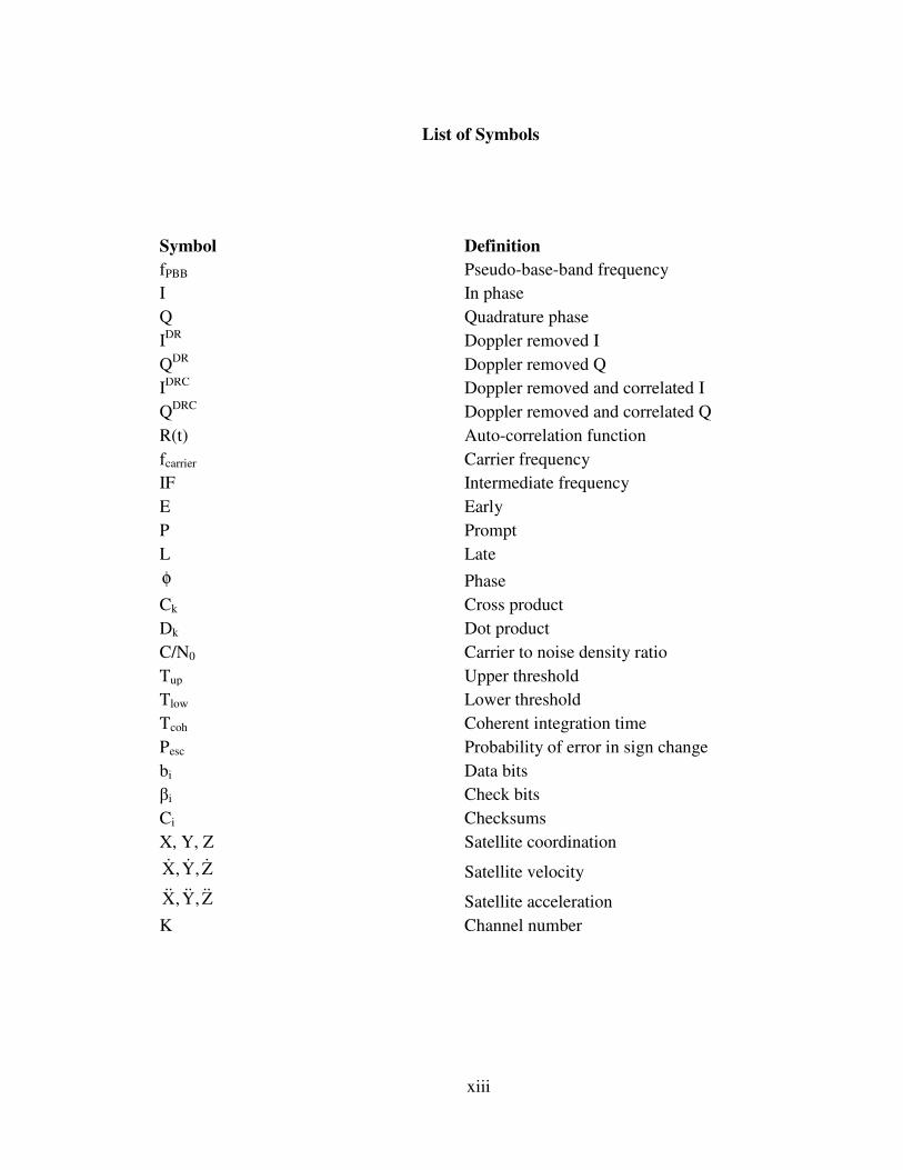
List of Symbols
Symbol Definition
fPBB Pseudo-base-band frequency
I In phase
Q Quadrature phase
IDR Doppler removed I
QDR Doppler removed Q
IDRC Doppler removed and correlated I
QDRC Doppler removed and correlated Q
R(t) Auto-correlation function
fcarrier Carrier frequency
IF Intermediate frequency
E Early
P Prompt
L Late
φ Phase
Ck Cross product
Dk Dot product
C/N0 Carrier to noise density ratio
Tup Upper threshold
Tlow Lower threshold
Tcoh Coherent integration time
Pesc Probability of error in sign change
bi Data bits
βi Check bits
Ci Checksums
X, Y, Z Satellite coordination
X,Y, Zɺ ɺ ɺ Satellite velocity
X,Y, Zɺɺ ɺɺ ɺɺ Satellite acceleration
K Channel number
xiv
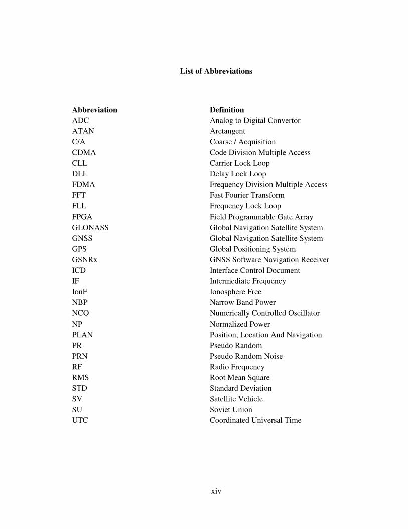
List of Abbreviations
Abbreviation Definition
ADC Analog to Digital Convertor
ATAN Arctangent
C/A Coarse / Acquisition
CDMA Code Division Multiple Access
CLL Carrier Lock Loop
DLL Delay Lock Loop
FDMA Frequency Division Multiple Access
FFT Fast Fourier Transform
FLL Frequency Lock Loop
FPGA Field Programmable Gate Array
GLONASS Global Navigation Satellite System
GNSS Global Navigation Satellite System
GPS Global Positioning System
GSNRx GNSS Software Navigation Receiver
ICD Interface Control Document
IF Intermediate Frequency
IonF Ionosphere Free
NBP Narrow Band Power
NCO Numerically Controlled Oscillator
NP Normalized Power
PLAN Position, Location And Navigation
PR Pseudo Random
PRN Pseudo Random Noise
RF Radio Frequency
RMS Root Mean Square
STD Standard Deviation
SV Satellite Vehicle
SU Soviet Union
UTC Coordinated Universal Time
1
CHAPTER ONE: INTRODUCTION
1.1 Chapter outline
In this Chapter, a general background of GPS and GLONASS systems is reviewed. Then,
the previous works related to this research is discussed. The Chapter continues with
defining the objective of this research. At the end of this Chapter, thesis outline is
presented.
1.2 Background
The Global Positioning System (GPS) provides accurate, continuous, worldwide, three
dimensional position and velocity information to users with the appropriate receiving
equipment (Spilker & Parkinson 1996). The GPS constellation nominally consists of 24
satellites arranged in six orbital planes with four satellites per plane. The satellites operate
in 20,200-km orbits at an inclination of 55°, and each satellite completes the orbit in
approximately 11 hours and 58 minutes. GPS can provide service to an unlimited number
of users. The satellite broadcast navigation data and ranging codes on two frequencies
using a technique called CDMA (Code Division Multiple Access). At the time of writing,
there are only two frequencies in use by the system, called L1 (1,575.42 MHz) and L2
2
(1,227.6 MHz). Each satellite transmits on these frequencies, but with a unique set of
codes compared to the other satellites. Each satellite generates a short code referred to as
the coarse/acquisition or C/A code and a long code denoted as the precision or P(Y) code.
Navigation data provides the means for the receiver to determine the location of the
satellite at the time of signal transmission. The ranging code enables the user’s receiver to
determine the transit time of the signal and hence determine the satellite-to-user range. If
the receiver clock were synchronized with the satellite clock, only three range
measurements would be required. However, a low cost quartz clock is usually employed
in navigation receivers to minimize the cost, complexity, and size of the receiver. Thus,
four measurements are required to determine the user latitude, longitude, height, and
receiver clock offset from internal system time.
The Russian counterpart of GPS is called GLONASS. GLONASS is a radio-based
satellite navigation system, developed by the former Soviet Union and now operated by
Russian Space Forces (Feairheller & Clark 2006).
The purpose of GLONASS is to provide an unlimited number of air, marine, and any
other type of users with all-weather three-dimensional positioning, velocity measuring
and timing anywhere in the world or near-earth space. A completely deployed
GLONASS constellation is composed of 24 satellites in three orbital planes. Eight
satellites are equally spaced in each plane. The satellites operate in circular 19,100-km
orbits at an inclination of 64.8°, and each satellite completes the orbit in approximately
11 hours and 15 minutes (GLONASS ICD 2002).
User equipment measures pseudorange and pseudorange rate of generally four or more
GLONASS satellites.
3
It also receives and processes navigation messages contained within navigation signals of
the satellites. The navigation message describes the position of the satellites. Processing
of the measurements and the navigation messages of the four or more GLONASS
satellites allow users to determine three position coordinates, three velocity vector
constituents, and to refer user time scale to the National Reference of Coordinated
Universal Time UTC (SU). The interface between the space segment and the user
equipment consists of radio links of L-band. At the time of writing, each GLONASS
satellite transmits navigation signals in two sub-bands of L-band (with centre frequency
of L1 ≈ 1.6 GHz and L2 ≈ 1.2 GHz). GLONASS uses FDMA (Frequency Division
Multiple Access) in both L1 and L2 sub-bands. This means that each satellite transmits a
navigation signal and raging code on its own carrier frequency in the L1 and L2 sub-
bands (Feairheller & Clark 2006). Two GLONASS satellites may transmit navigation
signals on the same carrier frequency if they are located in antipodal slots of a single
orbital plane. GLONASS satellites provide two types of ranging code signals in the L1
and L2 sub-bands: standard accuracy signal and high accuracy signal. The standard
accuracy signal is available for any users equipped with proper receivers and having
visible GLONASS system satellites above the horizon (GLONASS ICD 2002).
GLONASS consists of satellites in medium Earth orbit (MEO), a ground control
segment, and user equipment. GLONASS system was designed mainly for military
purposes and was fully deployed in 1995 with a constellation of 24 satellites without any
selective availability for civilian users (Polischuk & Revnivykh 2003). Commitments of
the Russian Government to sustain the free use of GLONASS for the following 10 years
were presented to the world community in 1995. However, between 1995 and the end of
4
1998, due to the lack of the federal budget funding, the GLONASS constellation was
degraded. By the Presidential Decree in 1999, GLONASS was used only in the Ministry
of Defense and Russian Aviation and Space Agency. After the evolution in the GNSS
industry, when Europe introduced Galileo for civilian use and GPS modernization, on
20th August 2001, the Russian Government adopted the long-term program of GLONASS
sustainment, modernization and application. The goal was to give more reliable and
accurate navigation solution in combination with other GNSS systems and to share this
market for civilian users (Polischuk & Revnivykh 2003).
While Russia’s economic problems have slowed its ability to replenish failing or failed
GLONASS satellites with the latest GLONASS-M models, Russia has continued to
update and distribute the public GLONASS Interface Control Document (ICD). The
GLONASS Coordination Scientific Information Center (KNITS), the Scientific and
Production Association of Applied Mechanics (NPO PM) and the Research Institute of
Space Device Engineering (RNII KP) must all agree on changes, additions, and
amendments to the ICD. The current ICD states that GLONASS is made available for all-
weather three-dimensional positioning, velocity measuring, and timing anywhere in the
world or near-earth space (Polischuk & Revnivykh 2003).
The largest GLONASS user community outside the Russian Federation is composed of
academics, engineers, geographers, cartographers, surveyors, and geologists who use
GLONASS for increased accuracy in surveying, mapping, and tracking earth movements
such as volcanoes, earthquakes, and glaciers (Leick 1995).
5
As designed, the ground support segments of GLONASS consists of a number of sites
scattered throughout Russia that control, track, and upload ephemeris, timing
information, and other data to satellites (Feairheller & Clark 2006).
Following the GLONASS modernization process, the second generation of GLONASS
satellites, GLONASS-M, was launched. After completing on-orbit tests, the first
GLONASS-M satellite was marked “healthy” on December 9, 2004, and is now
broadcasting a new civil L2 signal as well as additional GLONASS-M navigation data
that improves the performance of GLONASS significantly (Zinoviev 2005). The property
of having a civil L2 signal is very useful in achieving more reliable and accurate
navigation solution, because of the ability to mitigate ionosphere error in a dual
frequency GNSS systems. Moreover, a narrow band interference that affects L1 may not
affect L2. In total, with the help of the mentioned characteristics and other factors, the
accuracy of GLONASS-M navigation signal is 2-2.5 times better than the original
GLONASS navigation signal (Bartenev et al 2005).
GLONASS is on the way to its revival. The launches of third generation satellites,
GLONASS-K, will begin in 2010. Along with the extended life-time of 12 years,
GLONASS-K will be capable of broadcasting L3 civil signals, on which integrity
information for safety-of-life applications will be available (Zinoviev 2005).
It is clear that a GPS+GLONASS receiver might provide advantages over a single-system
(GPS-only or GLONASS-only) receiver (Ryan 2002), but in this integration, some issues
must be resolved. The most important issues are the differences in coordinate systems
and time reference frames between GPS and GLONASS channels (Zinoviev 2005).
6
GLONASS has better coverage in high latitudes because of its higher orbital inclination.
GPS coverage is superior near the equator (Chachis 2001).
The GPS system has begun the process of modernization to expand its capabilities to
include a new civilian code on the L2 frequency and eventually on the L5 frequency.
GLONASS has launched modernized satellites (GLONASS-M) and a new L3 signal in
GLONASS-K. In the near term, a receiver design will have to weigh the pros and cons of
developing complex hardware chips to take the advantage of the rapidly evolving signal
environment.
A software receiver can utilize the new signals without the need for a new hardware.
Given a suitable front-end, new frequencies and ranging codes can be used simply by
making software changes (Ledvina et al 2006). The software receiver idea is to use an
analog-to-digital converter (ADC) to change the input radio frequency (RF) signals into
digital data at the earliest possible stage in the receiver. In other words, the input signal is
digitized as close to the antenna as possible. Once the signal is digitized, software-based
digital signal processing will be used to obtain and process the digitized received signal.
The primary goal of the software receiver is to minimize the hardware used in a receiver.
A great flexibility can be achieved by using a software receiver (Bao & Tsui 2000a).
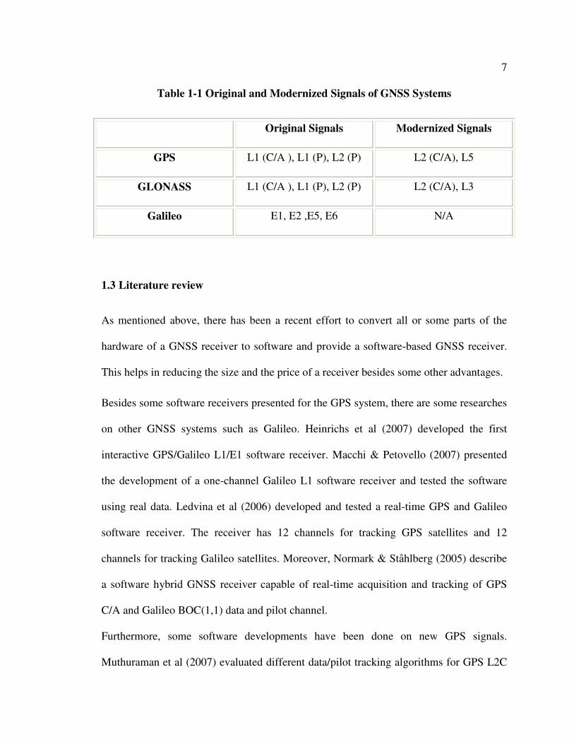
The following table shows the original and modernized signals of GPS, GLONASS, and
Galileo.
7
Table 1-1 Original and Modernized Signals of GNSS Systems
Original Signals Modernized Signals
GPS L1 (C/A ), L1 (P), L2 (P) L2 (C/A), L5
GLONASS L1 (C/A ), L1 (P), L2 (P) L2 (C/A), L3
Galileo E1, E2 ,E5, E6 N/A
1.3 Literature review
As mentioned above, there has been a recent effort to convert all or some parts of the
hardware of a GNSS receiver to software and provide a software-based GNSS receiver.
This helps in reducing the size and the price of a receiver besides some other advantages.
Besides some software receivers presented for the GPS system, there are some researches
on other GNSS systems such as Galileo. Heinrichs et al (2007) developed the first
interactive GPS/Galileo L1/E1 software receiver. Macchi & Petovello (2007) presented
the development of a one-channel Galileo L1 software receiver and tested the software
using real data. Ledvina et al (2006) developed and tested a real-time GPS and Galileo
software receiver. The receiver has 12 channels for tracking GPS satellites and 12
channels for tracking Galileo satellites. Moreover, Normark & Ståhlberg (2005) describe
a software hybrid GNSS receiver capable of real-time acquisition and tracking of GPS
C/A and Galileo BOC(1,1) data and pilot channel.
Furthermore, some software developments have been done on new GPS signals.
Muthuraman et al (2007) evaluated different data/pilot tracking algorithms for GPS L2C

8
signals using a software receiver. Ledvina et al (2005) demonstrated a real-time software
receiver operation for GPS L2 civilian signal. This GPS civilian L1/L2 software receiver
tracks 12 channels in real-time and has a navigation accuracy of 1-3 meters.
Some software receivers can be operated in a microprocessor, a Field-Programmable
Gate Array (FPGA) or Digital Signal Processor (DSP). Itaca is a scientific GNSS
software receiver (Tomatis et al 2007). The input data stream is processed by the
acquisition block, which is based on the Fast Fourier Transform (FFT). The tracking
block implements a coupled loop composed of a second order Costas Phase Lock Loop
(PLL) and a second order Delay Lock Loop (DLL). One advantage of this software is the
ability to monitor the signal at every stage. Since it was a part of Galileo receiver for high
dynamic application, it focuses on the Galileo and GPS more than other GNSS systems.
The software is going to be updated in order to make Itaca a valuable tool for the analysis
of the next generation of GNSS signals (Tomatis et al 2007). Namuru is the name given
to the open GNSS receiver research platform developed at the University of New South
Wales, Australia (Mumford et al 2006). The platform includes three aspects; 1) a custom
circuit board, 2) baseband processor (correlator block) logic design and 3) application
firmware. Both the circuit board and baseband processor designs are available in the
public domain. The custom circuit board has an L1 GPS RF front-end and contains an
Altera ´Cyclone´ FPGA chip, 3-axis accelerometer and various input/output and memory
components. The board has been carefully designed to keep noise around the sensitive RF
front-end as low as possible. This software uses a Frequency Locked Loop (FLL) for
carrier tracking. The cross product discriminator is used and the loop filter is a discrete
second-order filter. Code tracking is achieved with a first-order Delayed Locked Loop
9
(DLL) with carrier aiding. The dot product early-late discriminator is used with
bandwidth of 1 Hz (Mumford et al 2006).
A real-time GPS L1 C/A code software receiver has been implemented on a Digital
Signal Processor (DSP) by Humphreys et al (2006). The receiver exploits FFT-based
technique to perform acquisition. Efficient correlation algorithms and robust tracking
loops enable the receiver to track an equivalent of 43 L1 C/A code channels in real-time.
The FLL is used as a bridge between signal acquisition and Phase Locked Loop (PLL)
tracking. The first-order FLL employs a four-quadrant arctangent discriminator. The PLL
is a variable-bandwidth third-order Costas loop with a decision-directed discriminator
and the DLL is a standard first-order carrier-aided 0.5-Hz-bandwidth code tracking loop
with a dot product discriminator (Humphreys et al 2006). Kovar et al (2004) presented a
software receiver implemented in an FPGA. For this purpose, a two-channel RF unit, a
DSP unit based on FPGA device, and a high power computer unit are used. A powerful
FPGA called Virtex-II Pro from Xilinx is used to integrate all digital processing parts
(Kovar et al 2005). Spelat et al (2006) utilized FPGA and DSP for combined GPS and
Galileo software receiver. Although FPGAs are powerful, they are relatively expensive.
In addition, there is always a limitation for the capacity of the FPGA applied in this
research. It is possible that this FPGA does not have enough capacity for the integrated
GPS, GLONASS, and Galileo systems.
Won et al (2006) presented an efficient and practical way of general purpose high
performance signal tracking software for a multi-frequency GNSS receiver by using a
Maximum likelihood Estimation (MLE) technique. The cost function of the MLE for
estimating signal parameters such as code phase, carrier phase, and Doppler frequency is
10
used to derive a discriminator function for creating error signals from incoming and
reference signals. The designed MLE tracking algorithm is implemented in C++. The use
of C++ with Object-Oriented Programming (OOP) in combination with software
engineering techniques makes it possible to use the tracking software for multiple
frequencies and modulation schemes, for example, to track GPS and Galileo signals using
the same lines of source code. In addition, Petovello & Lachapelle (2006) presented an
efficient new method of Doppler removal and correlation with application to software-
based GNSS receivers.
The Purdue Software Receiver (PSR) is a real-time software GPS receiver developed at
the University of Purdue. The PSR is programmed in C++ and this has made the objects
to encapsulate functions and related data together and to reduce unnecessary copying of
data. The PSR has an FFT acquisition module presented in the code. The early and late
correlations are utilized to generate the early-minus-late (EML) signal, which enables
DLL tracking of the code. The prompt correlation is used directly for FLL/PLL tracking
of the carrier frequency (Heckler & Garrison 2004). The software receiver starts after the
acquisition card in the method proposed by Sharawi & Korniyenko (2007). The raw GPS
data which was collected on rooftop was sent to an RF front-end and then to a data
acquisition card that sampled the data and stored it on a hard drive. The whole software
receiver is provided using Matlab™ code. Although there is a claim on GLONASS
system on this research, no results for GLONASS are presented at the time of writing this
thesis.
The PLAN (Position, Location And Navigation) Group in the Department of Geomatics
Engineering at the University of Calgary developed its first software receiver
11
(GNSS_SoftRx™ ) in 2003 (Ma et al 2004 ). Numerous PLAN Group members (e.g.
Skone et al 2005, Zheng & Lachapelle 2005) have used the post-mission version of this
software for many research projects. The second version of the software was developed
in 2005. In this version, real-time operation capability was achieved by using optimized
algorithm to perform Doppler removal and code correlation (Charkhandeh et al 2006).
This receiver was expanded and optimized for a real-time acquisition method and
interfacing the software with hardware. Inside the recent GPS receiver, a second-order
loop filter DLL is used to track the C/A code of the signals. Carrier tracking is performed
using a second-order loop filter. The decision-directed cross product discriminator has
been implemented for FLL. An FLL-assisted PLL is also implemented in the receiver and
the ATAN carrier phase discriminator is used for the PLL (Charkhandeh et al 2006).
Petovello et al (2008) completed the software receiver in a modular design, wrote it
entirely in C++, and renamed it GSNRx™. This software operates in post-mission mode
and generates pseudorange; Doppler frequency and carrier phase observation for further
processing and generates a stand alone Position, Velocity and Time (PVT) solution.
These are just some examples of the research that have been done on GNSS software
receivers but none of the work mentioned above − either using a pure software receiver
or those implemented in microprocessor, FPGA or DPS − have presented a solution for
GLONASS system.
12
1.4 Research objective
The objective of this research is to develop a combined GPS and GLONASS software
receiver capable of providing a position solution. The software receiver generated in the
PLAN group at the Geomatics Engineering department of the University of Calgary
called GSNRx™ is modified to include the GLONASS system (Petovello et al 2008). To
this end, the following sub-objectives are identified:
1. Providing acquisition and tracking methods for GLONASS L1 and L2 signals,
2. Providing a method to decode GLONASS navigation data, and
3. Combining GLONASS with GPS in order to compute the best position solution
1.5 Thesis outline
In Chapter one, the GLONASS system background was presented. Moreover, the
previous researches in the relevant areas, along with their limitations, were described.
Finally, the objective of this thesis was presented.
In Chapter two, the historical evolution of GLONASS, its constellation and orbits are
discussed in detail. Because of the enhanced number of GLONASS-M satellites launches
and close plan for GLONASS-K satellites launches; these types of GLONASS satellites
are reviewed. The characteristics of GLONASS radio frequency signals including signal
structure, correlation characteristics, ranging code and navigation data bits are explained,
too. The objective of any Global Navigation Satellite System (GNSS) signal processing is
13
generating a local signal which exactly matches the incoming pseudo-base-band signal.
The signal processing procedure is as follows (Lachapelle 2007):
• Signal acquisition in which a local signal is generated and approximately matches
the incoming signal. GLONASS signal acquisition is explained in Chapter three.
• Signal tracking in which a local signal is generated in a way that closely matches
the incoming signal and GLONASS tracking steps are explained in Chapter four
for both GLONASS L1 and GLONASS L2 signals.
• Navigation message demodulation where the navigation data bits are decoded.
GLONASS navigation data demodulation is explained in Chapter five.
The combination of GPS and GLONASS for more accurate and reliable navigation
solution is explained in Chapter six. In the last Chapter, seven, the conclusion and
summary along with the future work are discussed.

14
CHAPTER TWO: GLONASS THEORY
2.1 Chapter outline
This Chapter begins with a short review of GLONASS history. Then, the GLONASS
orbit and constellation is briefly discussed. A short explanation of the legacy generation,
type M generation and type K generation GLONASS spacecraft is presented. The
Chapter continues with GLONASS signal characteristics and in this section the
GLONASS Radio Frequency (RF) signals in L-band, Pseudo Random (PR) ranging
codes, Intra-system interference and signals power level are explained. The GLONASS
navigation message in terms of its content and structure are then explained in detail. At
the end, the GLONASS time system and coordinate frame are discussed.
2.2 Historical evolution
The Soviet military initiated the GLONASS program in the mid-1970s to support military
requirements. The test of the system showed that they could use GLONASS for civilian
users while concurrently meeting the Soviet defense needs. The first GLONASS satellite
was launched in October 1982 and an initial test constellation of four satellites was
deployed by January 1984. However, the Soviet launched ballast payloads, instead of real
15
satellites, to save production costs, while the system was under development (Feairheller
& Clark 2006).
According to Feairheller & Clark 2006, in 1988, the free use of GLONASS navigation
signal was offered. In 1990-1991, after the demise of the Soviet Union, the Russians
tested the GLONASS constellation with 10-12 satellites. During the development, it
became clear that GLONASS signals interfered with radio astronomy observation in the
1610.6-1613.8 MHz band. The international scientific community protested and the
Russians agreed to modify the future GLONASS frequency plan in November 1993. In
April 1994, the Russians initiated the first of seven launches to complete the
constellation. In December 1995, the Russians successfully launched the last set of three
satellites to complete the 24-satellite constellation. In February 1995, these satellites were
declared operational and the constellation was fully populated for the first time. However,
a number of older satellites began to fail and constellation quickly degraded. From 1996
to 2001, the Russians only launched two sets of three satellites. This was insufficient to
maintain the constellation. The constellation degraded to six to eight satellites in 2001. In
August 2001, the Russian government passed Decree Number 587 entitled “Federal
Dedicated Program (FTsP) Global Navigation system-2002-2011.” This decree
established a 10-year program to rebuild the GLONASS program. The GLONASS FTsP
is a comprehensive program to fund the space segment, ground segment, user equipment,
manufacturing industry, transportation application industry, and geodetic application
industry. Under this program, the GLONASS constellation will be replenished with 10-
12 modernized GLONASS-M satellite and 18-27 new lightweight GLONASS-K
16
satellites. The first GLONASS-M satellite was launched in late 2003 (Feairheller & Clark
2006).
Moreover, GLONASS will continue to broadcast FDMA signals at its current frequencies
as well as new ones in the future at L3 (1201-1208 MHz) in CDMA format. Use of
FDMA signals has complicated the design of combined receivers, because all the other
GNSS receivers use CDMA. As a result, this equipment has been more expensive and
typically limited to professional or commercial application. Improved timing and orbit
determination are planned to enable the system to match GPS system performance by
2012. At the time of writing, GLONASS was in the seventh year of its 10-year plan for
rebuilding its constellation. Russia also plans to expand the GLONASS constellation
from the current fully operational capability (FOC) of 24 satellites to 30 satellites at a
minimum. Terrestrial and space-based augmentation systems are also under development
to improve real-time accuracy of GLONASS (GNSS Program Updates 2008).
At the time of writing, there are 20 GLONASS satellites in the constellation of which 19
are GLONASS-M satellites (GLONASS Constellation Status 2009).
Figure 2-1 shows GLONASS constellation status on 21th February 2009 (GLONASS
Constellation Status 2009).

17
Orbital
plane
Orbital
slot
RF
channel
#GC Operation
begins
Comments
2 01 728 20.01.09 In operation
3 05 727 17.01.09 In operation
4 06 795 29.01.04 In operation
6 01 701 08.12.04 Maintenance
7 05 712 07.10.05 In operation
I
8 06 729 12.02.09 In operation
9 -2 722 25.01.08 In operation
(L1 only)
10 04 717 03.04.07 In operation
11 00 723 22.01.08 In operation
13 -2 721 08.02.08 In operation
14 04 715 03.04.07 In operation
15 00 716 12.10.07 In operation
II
17 -1 718 04.12.07 In operation
18 -3 724 26.10.08 In operation
19 03 720 25.11.07 In operation
20 02 719 27.11.07 In operation
21 -1 725 05.11.08 In operation
22 -3 726 13.11.08 In operation
23 03 714 31.08.06 In operation
III
24 02 713 31.08.06 maintenance
Figure 2-1 GLONASS Constellation status on 21th
of February 2009

18
2.3 Constellation and orbit
The GLONASS constellation nominally consists of 21 active satellites plus three active
on-orbit spares. The 24 satellites will be uniformly located in three orbital planes 120°
apart in right ascension. A 21-satellite constellation provides continuous four-satellite
visibility over 97% of the Earth’s surface (Feairheller & Clark 2006). Under the
21-satellite concept, the performance of all 24 satellites will be determined by
GLONASS controllers and the best 21 will be activated. The remaining three will be held
for back up or in reserve.
Each GLONASS satellite is in a 19,100 km altitude circular orbit with an inclination of
64.8°. The orbital period is 11 hours and 15 minutes (GLONASS ICD 2002). The current
orbital configuration and overall system design provide navigation service to users up to
2,000 km above the Earth’s surface (Feairheller & Clark 2006).
Table 2-1 shows the difference between the nominal GPS and GLONASS constellations.
Table 2-1 GLONASS and GPS constellation comparison
GLONASS GPS
Number of satellite 24 24
Number of orbital plane 3 6
Orbital inclination 64.8° 55°
Period of revolution 11 h 15 m 11 h 58 m
Orbital altitude 19,100 km 20,200 km
19
2.4 Spacecraft description
At the time of writing, there are two types of GLONASS spacecraft in the constellation;
the first-generation GLONASS satellite and GLONASS-M satellites. As discussed
earlier, there will also be GLONASS-K satellites in the constellation in the next two
years. A brief explanation of each type is presented here.
2.4.1 First-generation GLONASS
From 1982, the Russians planned to launch the first generation of GLONASS satellites.
Although these are normally referred to as “GLONASS” satellites, the term “first-
generation GLONASS” is used herein to avoid confusion with the proper name of the
GNSS and from the use of “GLONASS satellite” to refer to any combination of satellites
within the system. The primary function of first-generation GLONASS satellites is
recording the satellite ephemeris and almanac data which are uploaded from ground
stations and also controlling of navigation signal formulation. Moreover, the onboard
clock has a critical role in all types of GLONASS satellites. The first-generation
GLONASS spacecraft carry three “Gem” cesium-beam frequency standards (Feairheller
& Clark 2006).
20
2.4.2 GLONASS-M
In 2003, the Russians began launching GLONASS-M satellites, where “M” stands for
“Modernized”. These satellites use more modern electronics and support a number of
new features. In comparison with the previous satellite, GLONASS-M offers some
advantages such as:
• Extended guaranteed life-time (seven vs. three years)
• More stable clock
• Additional GLONASS-M navigation data
• Inter-satellites radio link
One of the advantages of GLONASS-M satellite is the ability to transmit civil L2 signal
(Zinoviev 2005). Moreover, GLONASS-M satellites broadcast new navigation data and
have some differences relative to first-generation GLONASS satellite in both immediate
and non-immediate data. These new navigation data greatly improve overall system
performance (Zinoviev 2005).
2.4.3 GLONASS-K
The Russians plan to start launching the new GLONASS-K satellites in 2010. Currently,
there is a plan to produce 18-27 GLONASS-K satellites. These newer satellites weigh
about half of the GLONASS-M satellites. The lighter satellite will allow the Russians to
launch GLONASS-K satellites six at a time on a single Proton launch vehicle, or two at a
21
time on a Soyuz launch vehicle. GLONASS-K offers some advantages such as
(Feairheller & Clark 2006):
• Longer life-time, namely around 10-12 years
• More stable clock
• Third civil and military signals in the 1201-1208 MHz frequency range
2.5 GLONASS signal characteristics
In GPS, each satellite transmits the ranging code on the same frequency using Code
Division Multiple Access (CDMA). In GLONASS however, each satellite transmits the
same ranging code signal on different frequencies using Frequency Division Multiple
Access (FDMA) technique. Although there are some disadvantages in using an FDMA
technique such as larger and more expensive receivers because of the extra front-end
components to process multiple frequencies, some advantages are available. In particular,
a narrowband interference source that disrupts only one FDMA signal would disrupt all
CDMA signals simultaneously.
2.5.1 GLONASS navigation RF signal characteristics
The interface between space segment and user equipment consists of radio links of
L-band. Each GLONASS satellite transmits a navigation signal in two sub-bands of L-
band referred to as L1 and L2, the frequencies of which are defined by the following
expressions:
22
fk1 = f01 + K.∆f1 2-1
fk2 = f02 + K.∆f2 2-2
where K is the frequency number (frequency channel) of signals transmitted by
GLONASS satellites in the L1 and L2 sub-bands and
a) f01= 1602 MHz; ∆f1= 562.5 kHz, for L1 sub-band
b) f02= 1246 MHz; ∆f2= 437.5 kHz, for L2 sub-band
The channel number K for any particular GLONASS satellite is provided in the almanac
(non-immediate data of navigation message). K is a unique integer for each satellite and
varies from -07 to 13. The plan is to have satellites on opposite sides of the Earth
(antipodal) share the same frequency number.
Carrier frequencies L1 and L2 are generated from a common onboard time/frequency
standard in each satellite. The nominal value of this frequency is equal to 5.0 MHz
(GLONASS ICD 2002).
Figure 2-2 shows a general block diagram for generating GLONASS signals (Feairheller
& Clark 2006). As it is shown, this signal generator is for first-generation GLONASS
satellites which transmit standard accuracy signal on the L1 sub-band only. For
GLONASS-M satellites, standard accuracy signal must be added to the L2 sub-band.
23
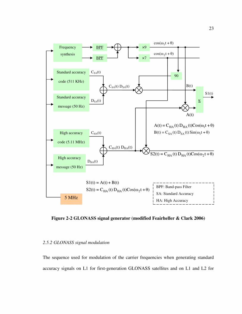
Figure 2-2 GLONASS signal generator (modified Feairheller & Clark 2006)
2.5.2 GLONASS signal modulation
The sequence used for modulation of the carrier frequencies when generating standard
accuracy signals on L1 for first-generation GLONASS satellites and on L1 and L2 for
θ)+tcos(ω1
θ)+tcos(ω2
Standard accuracy
message (50 Hz)
5 MHz
Frequency
synthesis
BPF
BPF
×9
×7
90
Σ
CSA(t)
B(t)
θ)+t(t)Cos(ωD (t)C=S2(t) 2HAHAθ)+t(t)Cos(ωD (t)C=S2(t) 2HAHA
Standard accuracy
code (511 KHz)
High accuracy
message (50 Hz)
High accuracy
code (5.11 MHz)
DSA(t)
CSA(t) DSA(t)
CHA(t)
DHA(t)
CHA(t) DHA(t)
A(t)A(t)
S1(t)
BPF: Band-pass Filter
SA: Standard Accuracy
HA: High Accuracy
B(t) + A(t)=S1(t) B(t) + A(t)=S1(t)
θ)+t(t)Cos(ωD (t)C=S2(t) 2HAHAθ)+t(t)Cos(ωD (t)C=S2(t) 2HAHA
θ)+t(t)Cos(ωD (t)C=A(t) 1HAHAθ)+t(t)Cos(ωD (t)C=A(t) 1HAHA
θ)+tSin(ω (t)D (t)C=B(t) 1SASA
24
GLONASS-M satellites is generated by modulo-2 addition of the flowing three binary
signals:
• Pseudo random (PR) standard accuracy ranging code transmitted at 511 kHz
• Navigation message transmitted at 50 Hz
• 100 Hz auxiliary meander sequence
2.5.3 GLONASS ranging code
GLONASS ranging code is a sequence of the maximum length (M-length) shift register.
GLONASS satellites provide two types of ranging code: standard accuracy and high
accuracy which are discussed in more details in next sections.
2.5.3.1 Standard accuracy ranging code
The standard accuracy signal is available for any users equipped with the proper receivers
and having a sufficient number of visible GLONASS system satellite above the horizon.
In fact, the standard accuracy code is designed for use by civil users worldwide.
(GLONASS ICD 2002).
Standard accuracy ranging code is sampled at the output of the 7th stage of a 9-stage shift
register. The initialization vector to generate this sequence is (111111111). The
generating polynomial which corresponds to the 9-stage shift register is:
G(X) = 1+X5+X9 2-3

25
A simplified block diagram of the standard accuracy ranging code generation is given in
Figure 2-3 (GLONASS ICD 2002).
Figure 2-3 Simplified block diagram of standard ranging code generation (from
GLONASS ICD 2002)
The GLONASS standard accuracy ranging code characteristics are shown in Table 2-2
(Beser & Danaher 1993).
Table 2-2 GLONASS standard accuracy ranging code characteristics
Code type M-length 9-bit shift register
Code rate 0.511 MHz
Code length 511 bits
Repeat rate 1 ms
Super-frame 2.5 minutes
Frame 30 seconds
Navigation message
String 2 seconds
26
The 511-bit code is clocked at 0.511 MHz and repeats every one millisecond. This short
code allows a receiver to search a maximum of 511 code phase shifts and consequently a
quick acquisition is achieved. Each code phase represents approximately 587 m
(Feairheller & Clark 2006).
The standard accuracy ranging code signal consists of a super-frame of 2.5 minutes
containing five frames of 30 second each. Each frame consists of 15 strings, each two
seconds long (Beser & Danaher 1993). More details regarding the navigation message are
given in section 2.6.
2.5.3.2 High accuracy ranging code
The Russians have not publicly published any specifics on high accuracy ranging code.
They have emphatically stated that this code is a military signal, and military signal is not
the interest of this thesis. Interested reader is referred to Feairheller & Clark 2006.
2.5.4 Intra-system interference
This interference is caused by inter-correlation properties of ranging code and FDMA
technique used in GLONASS system. When a navigation signal is transmitted on
frequency channel K=n, then in the receiver there is an interference between this signal
and signals transmitted on frequency channel K=n+1 and K=n-1. However, this
interference is conditional to the simultaneous visibility of the satellites with adjacent
frequencies (GLONASS ICD 2002).
27
2.5.5 Power level of the received signal
If the elevation mask is 5° or more, the power level of received GLONASS signal from
GLONASS satellite at the output of a 3 dBi linearly polarized antenna is not less than
-161 dBW for the L1 sub-band. For GLONASS-M satellites, the power is not less than
-161 dBW for L1 sub-band and not less than -167 dBW for L2 sub-band if the satellite is
observed at an angle of 5° or more (GLONASS ICD 2002). As such, the level of
GLONASS signal on L2 sub-band for GLONASS-M satellite is expected to be lower
than L1. This will have an impact on acquisition and tracking results. In other words,
acquisition and tracking of the L1 signal does not ensure acquisition and tracking of the
L2 signal from the same satellite.
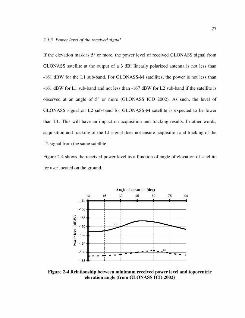
Figure 2-4 shows the received power level as a function of angle of elevation of satellite
for user located on the ground.
Figure 2-4 Relationship between minimum received power level and topocentric
elevation angle (from GLONASS ICD 2002)
28
2.6 GLONASS navigation message
The purpose of the navigation message is to provide users with requisite data for
positioning, timing and planning observations. The navigation message includes
immediate and non-immediate data transmitted at 50 bits per second.
The GLONASS navigation message is generated as continuously repeating super-frames.
A super-frame consists of frames and a frame consists of strings. Each of these units are
explained in detail in next sections.
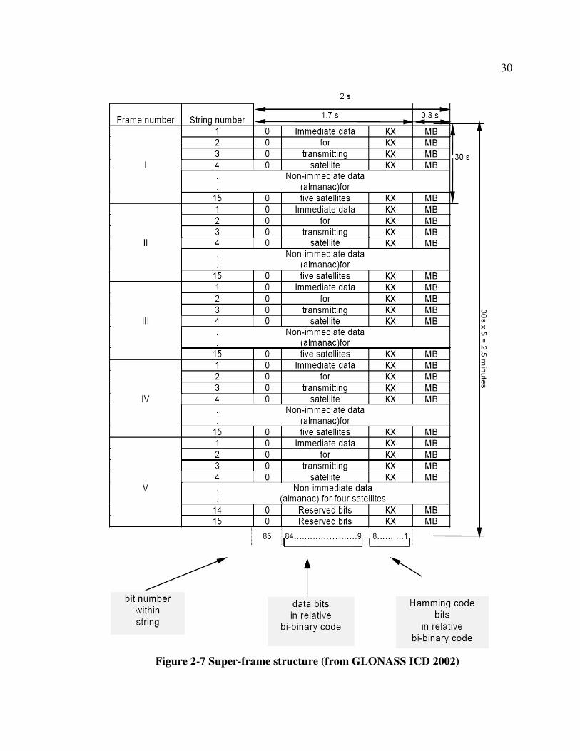
2.6.1 Super-frame structure
Within each super-frame, a total content of non-immediate data (almanac for 24
satellites) and the immediate data (for the satellite being tracked) are transmitted. Each
super-frame consists of five frames and has a duration of 2.5 minutes.
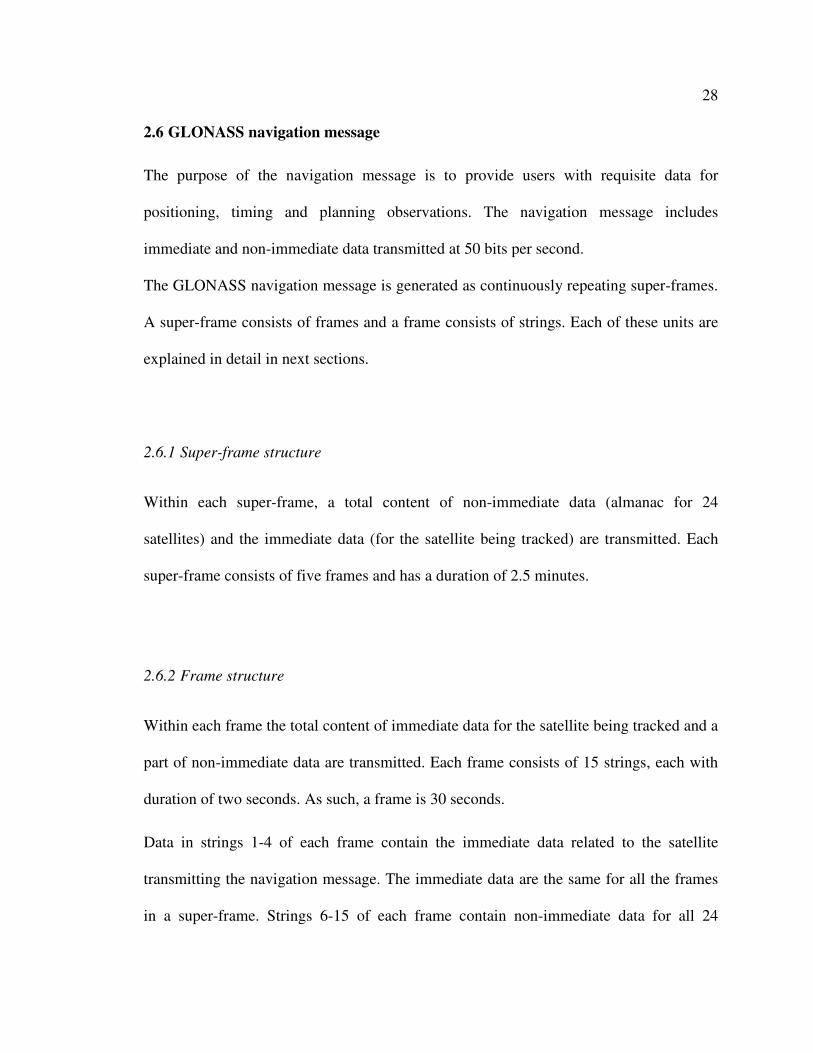
2.6.2 Frame structure
Within each frame the total content of immediate data for the satellite being tracked and a
part of non-immediate data are transmitted. Each frame consists of 15 strings, each with
duration of two seconds. As such, a frame is 30 seconds.
Data in strings 1-4 of each frame contain the immediate data related to the satellite
transmitting the navigation message. The immediate data are the same for all the frames
in a super-frame. Strings 6-15 of each frame contain non-immediate data for all 24
29
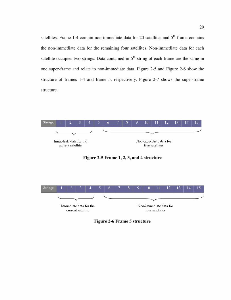
satellites. Frame 1-4 contain non-immediate data for 20 satellites and 5th frame contains
the non-immediate data for the remaining four satellites. Non-immediate data for each
satellite occupies two strings. Data contained in 5th string of each frame are the same in
one super-frame and relate to non-immediate data. Figure 2-5 and Figure 2-6 show the
structure of frames 1-4 and frame 5, respectively. Figure 2-7 shows the super-frame
structure.
Figure 2-5 Frame 1, 2, 3, and 4 structure
Figure 2-6 Frame 5 structure
30
Figure 2-7 Super-frame structure (from GLONASS ICD 2002)
31
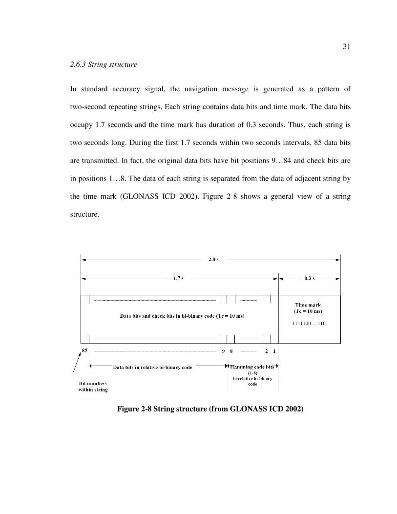
2.6.3 String structure
In standard accuracy signal, the navigation message is generated as a pattern of
two-second repeating strings. Each string contains data bits and time mark. The data bits
occupy 1.7 seconds and the time mark has duration of 0.3 seconds. Thus, each string is
two seconds long. During the first 1.7 seconds within two seconds intervals, 85 data bits
are transmitted. In fact, the original data bits have bit positions 9…84 and check bits are
in positions 1…8. The data of each string is separated from the data of adjacent string by
the time mark (GLONASS ICD 2002). Figure 2-8 shows a general view of a string
structure.
Figure 2-8 String structure (from GLONASS ICD 2002)
32
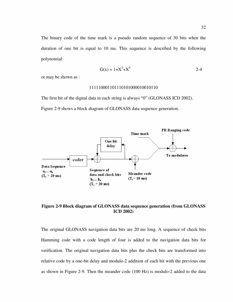
The binary code of the time mark is a pseudo random sequence of 30 bits when the
duration of one bit is equal to 10 ms. This sequence is described by the following
polynomial:
G(x) = 1+X3+X5 2-4
or may be shown as :
111110001101110101000010010110
The first bit of the digital data in each string is always “0” (GLONASS ICD 2002).
Figure 2-9 shows a block diagram of GLONASS data sequence generation.
Figure 2-9 Block diagram of GLONASS data sequence generation (from GLONASS
ICD 2002)
The original GLONASS navigation data bits are 20 ms long. A sequence of check bits
Hamming code with a code length of four is added to the navigation data bits for
verification. The original navigation data bits plus the check bits are transformed into
relative code by a one-bit delay and modulo-2 addition of each bit with the previous one
as shown in Figure 2-9. Then the meander code (100 Hz) is modulo-2 added to the data
33
bits. Because of the effect of meander code, the data bit duration is now 10 ms. Time
mark bits which are 10 ms long are appended to the data bits, thus generating the two-
second long string. The string is sent to the modulator for modulation with standard
accuracy ranging code.
2.6.4 Navigation message content
According to GLONASS ICD 2002, the navigation message includes immediate data and
non-immediate data.
Immediate data relates specifically to the GLONASS satellite broadcasting the data and
includes:
• Difference between onboard time scale of satellite and GLONASS time
• Relative difference between carrier frequency of the satellite and its nominal
value
• Ephemeris parameters
The non-immediate data contain almanac of the system and includes:
• Data on status of all satellites within space segment
• Coarse correction to the onboard time scale of each satellite relative to GLOASS
time
• Orbital parameters of all satellites within space segment
• Correction to GLONASS time relative to UTC (SU)

34
2.7 GLONASS time
GLONASS satellites are equipped with clocks which exhibit a daily instability not worse
than 5×10-13 for first-generation GLONASS satellites and 1×10-14 for the GLONASS-M
satellites. GLONASS time can be defined as (GLONASS ICD 2002):
tGLONASS = UTC(SU) + 03 hours 00 minutes 2-5
To re-compute satellite ephemeris at the moment of measurement in UTC(SU) the
following equation shall be used:
tGLONASS = t + τc + τn (tb) - γn(tb)(t-tb) 2-6
where ‘t’ is time of transmission of the navigation signal in the onboard time scale. ‘τc’ is
the GLONASS time scale correction to UTC (SU) time. ‘τn(tb)’ is the correction to nth
satellite time relative to GLONASS time at time tb. ‘γn(tb)’ is the relative deviation of
predicted carrier frequency value of n-satellite from nominal value at time tb (GLONASS
ICD 2002).
2.8 GLONASS reference frame
Before 1993, GLONASS provided data in the Soviet Geodetic System 1985 (SGS-85).
From August 1993 to September 2007, GLONASS transmitted ephemeris data in the
Earth Parameter System 1990 (PZ-90). PZ-90 is similar in quality to the Earth model
employed in WGS-84 used by GPS (Feairheller & Clark 2006). The origin of this frame
is located at the centre of the Earth’s mass. The Z-axis is directed to the Conventional
Terrestrial Pole as recommended by the International Earth Rotation Service (IERS). The
X-axis is directed to the point of intersection of the Earth’s equatorial plane and the zero
35
meridians. The Y-axis completes coordinate system to the right-handed one (GLONASS
ICD 2002).
In June 2007, Russian government decided on the implementation of PZ-90.02. Thus,
from 20 September 2007, GLONASS satellites broadcast ephemeris information in
PZ-90.02 reference frame. With the new system, the GLONASS orbit accuracy is
improved by 15-25%. To transform PZ-90.02 coordination to ITRF (Inertial Terrestrial
Reference Frame) no rotation is needed but an offset of -36 cm, +8 cm, and +18 cm in the
X,Y and Z directions is required (Revnivykh 2007). On the other hand, the WGS-84
reference frame and ITRF closely match. As such, a transformation from PZ-90.02 to
WGS-84 can be provided.
36
CHAPTER THREE: ACQUISITION
3.1 Chapter outline
In this Chapter a general view of a GNSS receiver is presented. The incoming GNSS
signal structure and the process on it, is explained. Then, the acquisition theory is briefly
discussed and a few acquisition methods are reviewed. The differences between GPS and
GLONASS signals affecting acquisition are highlighted. At the end, a data collection set-
up is described and some acquisition results are presented.
3.2 GNSS receiver overview
The final goal of a GNSS receiver is computing the position and velocity of the receiver
or at least providing some measurements which can be used to compute these values. For
this purpose, the received signals at antenna must be acquired and tracked. After tracking,
navigation message can be extracted and utilized to generate some measurements that are
useful in computing the navigation solution.
Figure 3-1 illustrates a block diagram of a GNSS receiver. The received signal at the
antenna is amplified and then down converted to the desired intermediate frequency (IF).
The down converted signal is sampled and sent to the signal processor block.
Amplification, down conversion and sampling are performed in the radio frequency (RF)
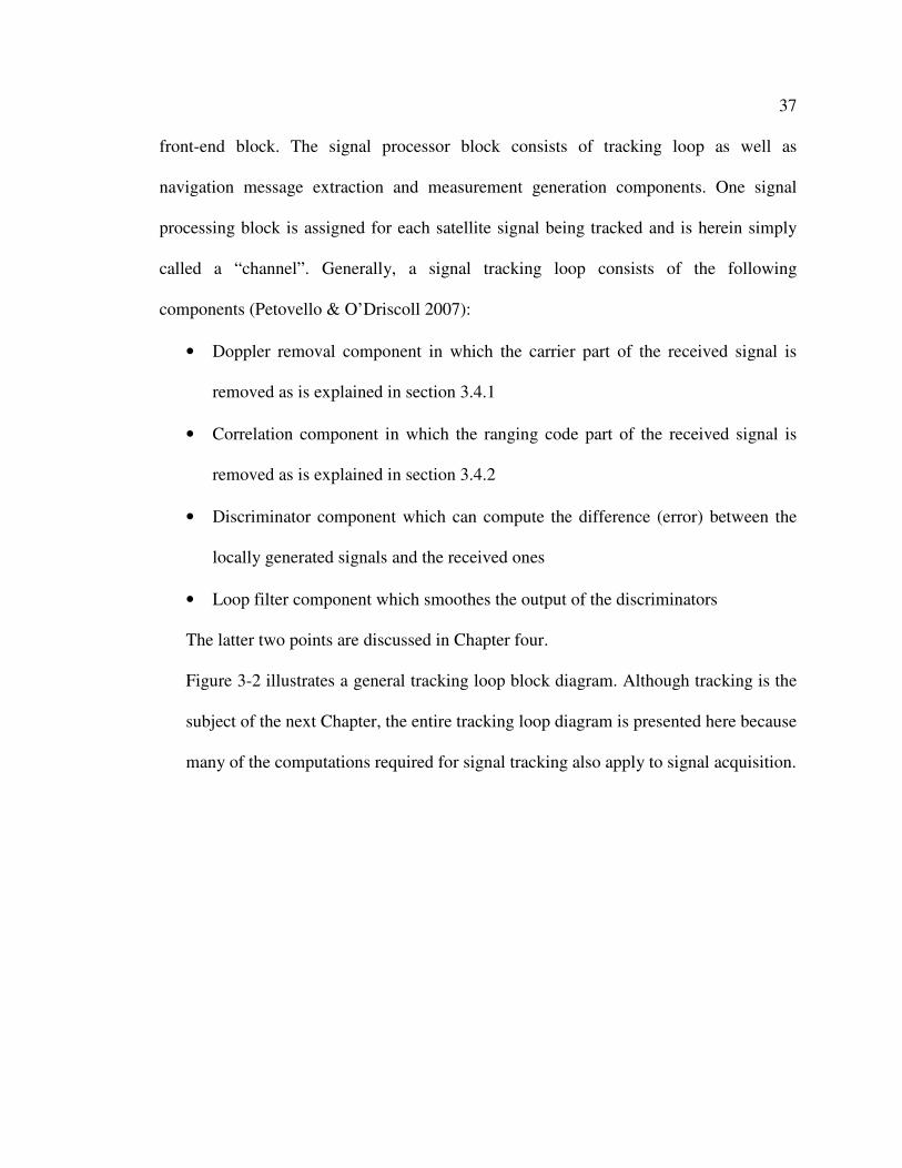
37
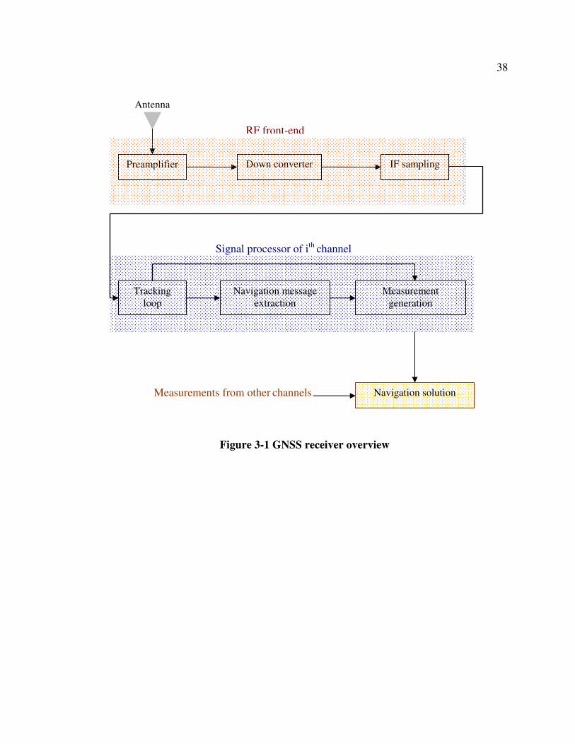
front-end block. The signal processor block consists of tracking loop as well as
navigation message extraction and measurement generation components. One signal
processing block is assigned for each satellite signal being tracked and is herein simply
called a “channel”. Generally, a signal tracking loop consists of the following
components (Petovello & O’Driscoll 2007):
• Doppler removal component in which the carrier part of the received signal is
removed as is explained in section 3.4.1
• Correlation component in which the ranging code part of the received signal is
removed as is explained in section 3.4.2
• Discriminator component which can compute the difference (error) between the
locally generated signals and the received ones
• Loop filter component which smoothes the output of the discriminators
The latter two points are discussed in Chapter four.
Figure 3-2 illustrates a general tracking loop block diagram. Although tracking is the
subject of the next Chapter, the entire tracking loop diagram is presented here because
many of the computations required for signal tracking also apply to signal acquisition.
38
Figure 3-1 GNSS receiver overview
Antenna
Preamplifier Down converter IF sampling
Tracking
loop
Navigation message
extraction
Measurement
generation
Navigation solution
RF front-end
Signal processor of ith channel
Measurements from other channels
39
Figure 3-2 General signal tracking block diagram (modified Petovello & O’Driscoll
2007)
3.3 Incoming GNSS signal structure
In this section, the incoming signal structure is overviewed. Furthermore, the signal
processing steps from the antenna to the sampling is explained.
Generally, a GNSS signal structure can be presented by the following equation
(Lachapelle 2007):
RS(t) A.C(t).D(t).cos(2 f t )= π + φ 3-1
where
• S(t) represents the signal received at the antenna,
• A represents the amplitude of the received signal,
• C(t) represents the received ranging code,
Doppler Removal
Carrier Generation
Correlation
Code Generation
Code Discriminator
Carrier
Loop Filter
Carrier Discriminator
Code Loop Filter
Samples from RF front-end
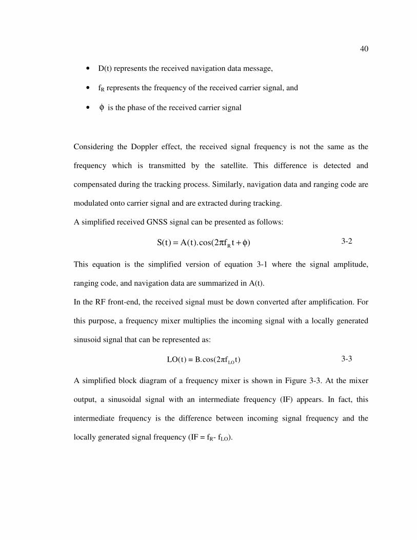
40
• D(t) represents the received navigation data message,
• fR represents the frequency of the received carrier signal, and
• φ is the phase of the received carrier signal
Considering the Doppler effect, the received signal frequency is not the same as the
frequency which is transmitted by the satellite. This difference is detected and
compensated during the tracking process. Similarly, navigation data and ranging code are
modulated onto carrier signal and are extracted during tracking.
A simplified received GNSS signal can be presented as follows:
RS(t) A(t).cos(2 f t )= π + φ 3-2
This equation is the simplified version of equation 3-1 where the signal amplitude,
ranging code, and navigation data are summarized in A(t).
In the RF front-end, the received signal must be down converted after amplification. For
this purpose, a frequency mixer multiplies the incoming signal with a locally generated
sinusoid signal that can be represented as:
LOLO(t) = B.cos(2πf t) 3-3
A simplified block diagram of a frequency mixer is shown in Figure 3-3. At the mixer
output, a sinusoidal signal with an intermediate frequency (IF) appears. In fact, this
intermediate frequency is the difference between incoming signal frequency and the
locally generated signal frequency (IF = fR- fLO).
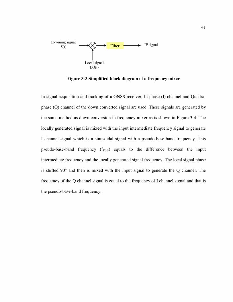
41
Figure 3-3 Simplified block diagram of a frequency mixer
In signal acquisition and tracking of a GNSS receiver, In-phase (I) channel and Quadra-
phase (Q) channel of the down converted signal are used. These signals are generated by
the same method as down conversion in frequency mixer as is shown in Figure 3-4. The
locally generated signal is mixed with the input intermediate frequency signal to generate
I channel signal which is a sinusoidal signal with a pseudo-base-band frequency. This
pseudo-base-band frequency (fPBB) equals to the difference between the input
intermediate frequency and the locally generated signal frequency. The local signal phase
is shifted 90° and then is mixed with the input signal to generate the Q channel. The
frequency of the Q channel signal is equal to the frequency of I channel signal and that is
the pseudo-base-band frequency.
Filter Incoming signal
S(t)
Local signal
IF signal
LO(t)

42
Figure 3-4 I and Q signal generation (modified Lachapelle 2007)
The final step in an RF front-end is to sample the continuous signal with a sampling
frequency fs (= 1/Ts). Therefore, the kth complex samples at the output of RF front-end
are raw
kI and raw
kQ and can be defined as:
raw
k s k k k PBB s
raw
k s k k k PBB s
I = I(kT ) = A .D .C .cos(2 f kT + )
Q = Q(kT ) = A .D .C .sin(2 f kT + )
π φ
π φ
3-4
The superscript “raw” is chosen for these samples because these are unprocessed samples
which are transmitted to the signal processor block for Doppler removal and correlation.
For the purpose of this paper, the data bits are assumed constant during an integration
interval and will therefore be omitted from the following equations
Filter
Down converted
signal
cos(2πfIFt)
In-phase signal
Local signal
90°
Filter Quadra-phase signal
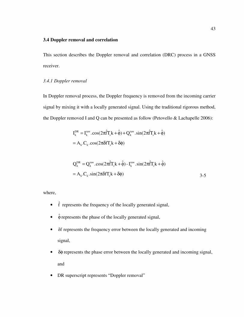
43
3.4 Doppler removal and correlation
This section describes the Doppler removal and correlation (DRC) process in a GNSS
receiver.
3.4.1 Doppler removal
In Doppler removal process, the Doppler frequency is removed from the incoming carrier
signal by mixing it with a locally generated signal. Using the traditional rigorous method,
the Doppler removed I and Q can be presented as follow (Petovello & Lachapelle 2006):
DR raw raw
k k s k s
k k s
DR raw raw
k k s k s
k k s
ˆ ˆˆ ˆI I .cos(2 fT k ) Q .sin(2 fT k )
A .C .cos(2 fT k )
ˆ ˆˆ ˆQ Q .cos(2 fT k ) - I .sin(2 fT k )
A .C .sin(2 fT k )
= π + φ + π + φ
= πδ + δφ
= π + φ π + φ
= πδ + δφ
3-5
where,
• f represents the frequency of the locally generated signal,
• φ represents the phase of the locally generated signal,
• δf represents the frequency error between the locally generated and incoming
signal,
• δφ represents the phase error between the locally generated and incoming signal,
and
• DR superscript represents “Doppler removal”
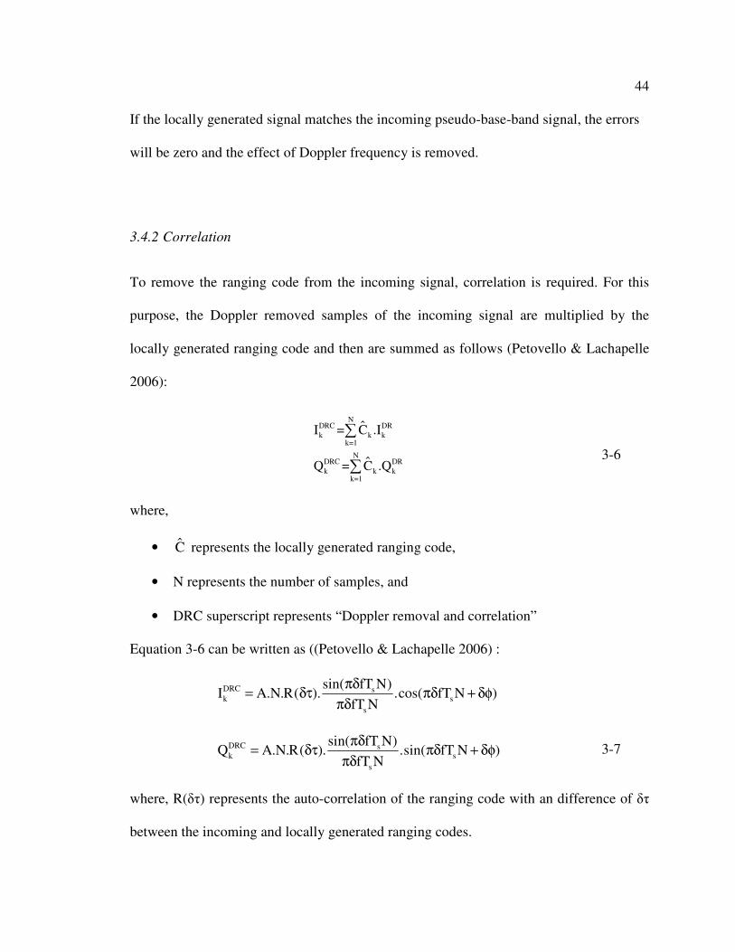
44
If the locally generated signal matches the incoming pseudo-base-band signal, the errors
will be zero and the effect of Doppler frequency is removed.
3.4.2 Correlation
To remove the ranging code from the incoming signal, correlation is required. For this
purpose, the Doppler removed samples of the incoming signal are multiplied by the
locally generated ranging code and then are summed as follows (Petovello & Lachapelle
2006):
NDRC DR
k k kk=1
NDRC DR
k k kk=1
ˆI = C .I
ˆQ = C .Q
∑
∑
3-6
where,
• C represents the locally generated ranging code,
• N represents the number of samples, and
• DRC superscript represents “Doppler removal and correlation”
Equation 3-6 can be written as ((Petovello & Lachapelle 2006) :
DRC sk s
s
DRC sk s
s
sin( fT N)I A.N.R( ). .cos( fT N )
fT N
sin( fT N)Q A.N.R( ). .sin( fT N )
fT N
πδ= δτ πδ + δφ
πδ
πδ= δτ πδ + δφ
πδ
3-7
where, R(δτ) represents the auto-correlation of the ranging code with an difference of δτ
between the incoming and locally generated ranging codes.
45
3.5 GNSS signal acquisition
Acquisition is the process of detecting the presence of a GNSS signal. When the signal is
detected, the necessary parameters can be obtained and passed to the tracking process
described in Chapter four.
A variety of GNSS signal acquisition methods are presented in different references (e.g.
Ward et al 2006; Bao & Tsui 2000b, Van Dierendonck 1996). Bao & Tsui (2000b)
present the cell-by-cell search, the fast Fourier transformation (FFT), and the delay and
multiplication method for GNSS signal acquisition. Each method has some advantages
and disadvantages. For example, the delay and multiplication method is faster than FFT
method but in case of weak signals, it has a lower performance. Therefore, there is a
trade-off between speed and sensitivity. If the signal is strong, the fast-low sensitivity
acquisition method can detect it but if the signal is weak, the FFT method is better able to
find it (Bao & Tsui 2000b). However, in case of weak signals, some other methods are
presented (e.g. O’Driscoll 2007, Psiaki 2001). For the purpose of this work, only the cell-
by-cell search method and FFT method are explained in next sections.
3.5.1 Cell-by-cell search method
In the cell-by-cell search method, the correlation is performed in the time domain, where
the locally generated ranging code is shifted and accumulated for all possible shifts.
Therefore, for GPS signal acquisition, all 1023 C/A ranging code chips are examined.
Typically, code chip is searched in increments of half chip and each code phase value to
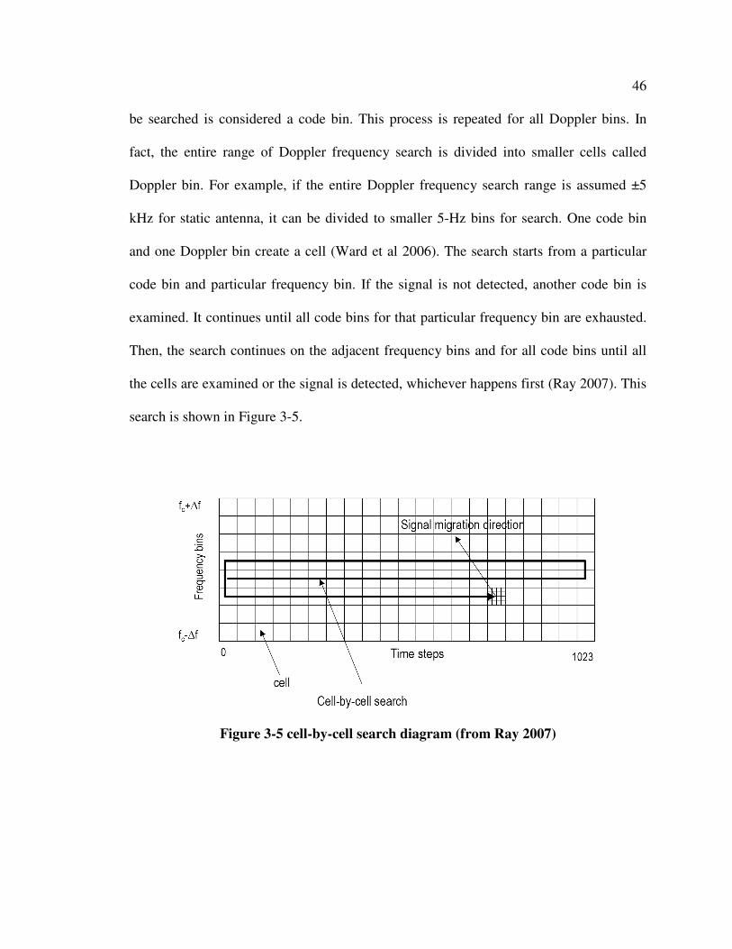
46
be searched is considered a code bin. This process is repeated for all Doppler bins. In
fact, the entire range of Doppler frequency search is divided into smaller cells called
Doppler bin. For example, if the entire Doppler frequency search range is assumed ±5
kHz for static antenna, it can be divided to smaller 5-Hz bins for search. One code bin
and one Doppler bin create a cell (Ward et al 2006). The search starts from a particular
code bin and particular frequency bin. If the signal is not detected, another code bin is
examined. It continues until all code bins for that particular frequency bin are exhausted.
Then, the search continues on the adjacent frequency bins and for all code bins until all
the cells are examined or the signal is detected, whichever happens first (Ray 2007). This
search is shown in Figure 3-5.
Figure 3-5 cell-by-cell search diagram (from Ray 2007)
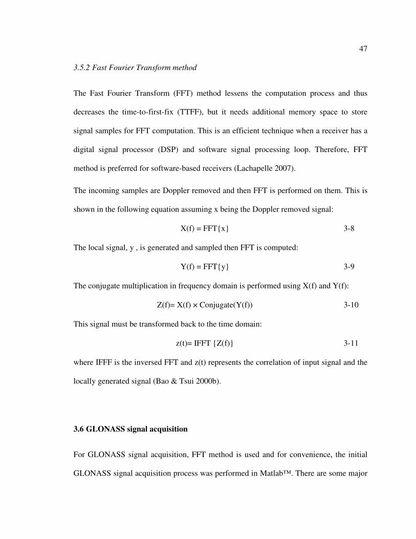
47
3.5.2 Fast Fourier Transform method
The Fast Fourier Transform (FFT) method lessens the computation process and thus
decreases the time-to-first-fix (TTFF), but it needs additional memory space to store
signal samples for FFT computation. This is an efficient technique when a receiver has a
digital signal processor (DSP) and software signal processing loop. Therefore, FFT
method is preferred for software-based receivers (Lachapelle 2007).
The incoming samples are Doppler removed and then FFT is performed on them. This is
shown in the following equation assuming x being the Doppler removed signal:
X(f) = FFT{x} 3-8
The local signal, y , is generated and sampled then FFT is computed:
Y(f) = FFT{y} 3-9
The conjugate multiplication in frequency domain is performed using X(f) and Y(f):
Z(f)= X(f) × Conjugate(Y(f)) 3-10
This signal must be transformed back to the time domain:
z(t)= IFFT {Z(f)} 3-11
where IFFF is the inversed FFT and z(t) represents the correlation of input signal and the
locally generated signal (Bao & Tsui 2000b).
3.6 GLONASS signal acquisition
For GLONASS signal acquisition, FFT method is used and for convenience, the initial
GLONASS signal acquisition process was performed in Matlab™. There are some major
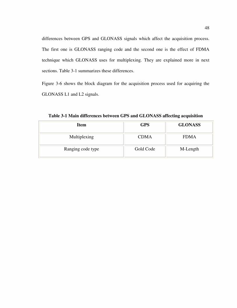
48
differences between GPS and GLONASS signals which affect the acquisition process.
The first one is GLONASS ranging code and the second one is the effect of FDMA
technique which GLONASS uses for multiplexing. They are explained more in next
sections. Table 3-1 summarizes these differences.
Figure 3-6 shows the block diagram for the acquisition process used for acquiring the
GLONASS L1 and L2 signals.
Table 3-1 Main differences between GPS and GLONASS affecting acquisition
Item GPS GLONASS
Multiplexing CDMA FDMA
Ranging code type Gold Code M-Length
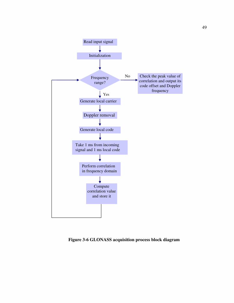
49
Figure 3-6 GLONASS acquisition process block diagram
Read input signal
Initialization
Frequency range?
Generate local carrier
Doppler removal
Yes
Compute correlation value
and store it
Take 1 ms from incoming signal and 1 ms local code
Generate local code
Perform correlation in frequency domain
No Check the peak value of correlation and output its code offset and Doppler
frequency
50
3.6.1 Effect of ranging code
As discussed in section 2.5.3, the GLONASS ranging code is different from GPS ranging
code. In fact, all the GLONASS satellites in the constellation transmit the same ranging
code; however each GPS satellite has a unique ranging code. GPS C/A ranging code
signal belongs to a family of Pseudo Random Noise (PRN) codes which are called Gold
codes. These codes are generated from the product of the output of two maximum length
10-stage shift registers which are driven by a 1.023 MHz clock and each one includes
1023 bits (Spilker 1996). On the other hand, GLONASS ranging code is not a Gold code
but is a maximum length 9-stage shift register sequence. A maximum length sequence is
a type of pseudo random binary sequence which is generated from an m-stage shift
register with linear feedback. In maximum length sequence, an m-stage shift register
produces a sequence with the length of 2m-1. In case of GLONASS ranging code, because
the shift register has nine stages, a 511-bit sequence is generated (29-1= 511). The auto-
correlation of a GLONASS ranging code takes two values: 511 and -1.
For GLONASS signal acquisition, one and only one ranging code must be generated for
all the GLONASS satellites as a replica ranging code.
3.6.2 Effect of FDMA
GLONASS uses Frequency Division Multiple Access technique. This means that each
satellite transmits its own carrier frequency. For this purpose, the carrier frequency with
channel number zero (i.e., 1602.00 MHz) is down converted to intermediate frequency
51
(IF) in the front-end as discussed in section 3.2 and the other GLONASS satellites’
carrier frequencies are generated accordingly:
1or2∆f×K+IF=Carrierf 3-12
where,
• IF is the intermediate frequency,
• K is the channel number, and
• ∆f1or2 is the frequency offset for GLONASS L1 and L2 as is discussed in section
2.5.1.
Considering that each GLONASS satellite is transmitting its own frequency, some of the
Doppler removal and correlation methods which are used for GPS can not be
implemented for GLONASS. For example, in look-up table Doppler removal and
correlation method, the sine and cosine values of the possible phases are generated and
stored in a table (Charkhandeh et al 2006). This provides considerable processing
improvements because the local carrier phase does not need to be generated on the fly.
For GLONASS however, the desired sine and cosine values must either be computed on
the fly which is not efficient for real-time operation, or a separate table must be used for
every GLONASS satellite. Although the latter is possible, it requires considerable
memory requirements and was therefore avoided in this case..
Moreover, in the simultaneous Doppler removal method for GPS presented by Petovello
& Lachapelle (2006), instead of a look-up table, a single frequency table is generated.
Considering that only one locally generated frequency is used for Doppler removal of all
the GPS satellites, it is required that the removal be performed just once for all the
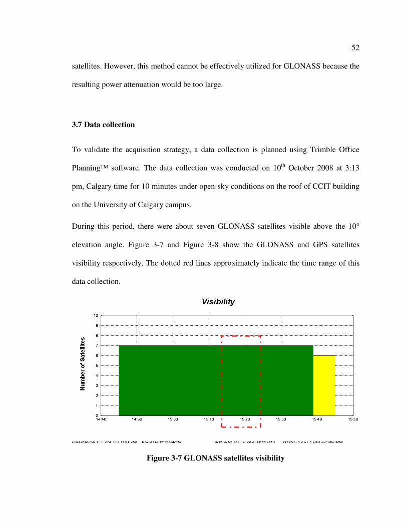
52
satellites. However, this method cannot be effectively utilized for GLONASS because the
resulting power attenuation would be too large.
3.7 Data collection
To validate the acquisition strategy, a data collection is planned using Trimble Office
Planning™ software. The data collection was conducted on 10th October 2008 at 3:13
pm, Calgary time for 10 minutes under open-sky conditions on the roof of CCIT building
on the University of Calgary campus.
During this period, there were about seven GLONASS satellites visible above the 10°
elevation angle. Figure 3-7 and Figure 3-8 show the GLONASS and GPS satellites
visibility respectively. The dotted red lines approximately indicate the time range of this
data collection.
Figure 3-7 GLONASS satellites visibility
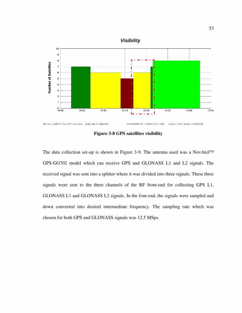
53
Figure 3-8 GPS satellites visibility
The data collection set-up is shown in Figure 3-9. The antenna used was a NovAtel™
GPS-GG702 model which can receive GPS and GLONASS L1 and L2 signals. The
received signal was sent into a splitter where it was divided into three signals. These three
signals were sent to the three channels of the RF front-end for collecting GPS L1,
GLONASS L1 and GLONASS L2 signals. In the font-end, the signals were sampled and
down converted into desired intermediate frequency. The sampling rate which was
chosen for both GPS and GLONASS signals was 12.5 MSps.

54
Figure 3-9 Data collection set-up
3.8 Acquisition results
The GPS signals acquired by the FFT method are presented in Table 3-2. Figure 3-10
shows the elevation angle of each GPS satellite during the data collection period. The L1
signal for all the visible GPS satellites was acquired except G15 and G14 which were
below 10° elevation angle and so weak. Although, the L1 signals for almost all GPS
satellites at elevation angle below 10° were acquired, these signals are weak and during
the tracking process may lose lock.
GLONASS SV GPS SV
Splitter
GPS L1
GLONASS L1
GLONASS L2
RF Front-end
Antenna
date: 10th October 2008
time: 3:13 pm, Calgary time
duration: 10 minutes
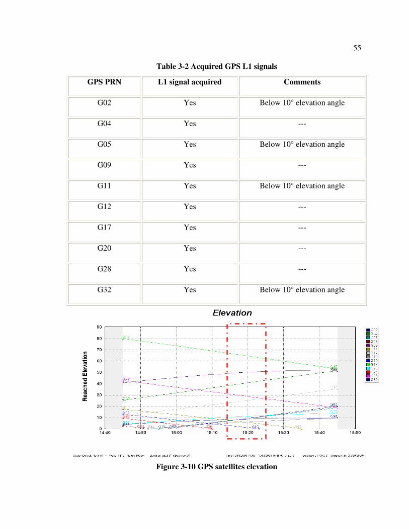
55
Table 3-2 Acquired GPS L1 signals
GPS PRN L1 signal acquired Comments
G02 Yes Below 10° elevation angle
G04 Yes ---
G05 Yes Below 10° elevation angle
G09 Yes ---
G11 Yes Below 10° elevation angle
G12 Yes ---
G17 Yes ---
G20 Yes ---
G28 Yes ---
G32 Yes Below 10° elevation angle
Figure 3-10 GPS satellites elevation

56
Table 3-3 shows the acquired GLONASS L1 and L2 signals. It is noted that the L2 signal
of GLONASS satellite at orbital slot 07 is not acquired because this satellite is in low
elevation and its L1 and L2 signals are weak. Generally, GLONASS L2 signal is weaker
than GLONASS L1 signal as discussed in section 2.5.5. Therefore, although L1 is
acquired, L2 can not be detected in this case.
Figure 3-11 shows the elevation angle of each GLONASS satellite during the data
collection period.
Table 3-3 Acquired GLONASS L1 and L2 signals
Orbital
slot
Channel
Number
L1 signal
acquired
L2 signal
acquired
SV
type
R07 05 Yes No M
R13 -2 Yes Yes M
R15 00 Yes Yes M
R17 -1 Yes Yes M
R23 03 Yes Yes M
R24 02 Yes Yes M
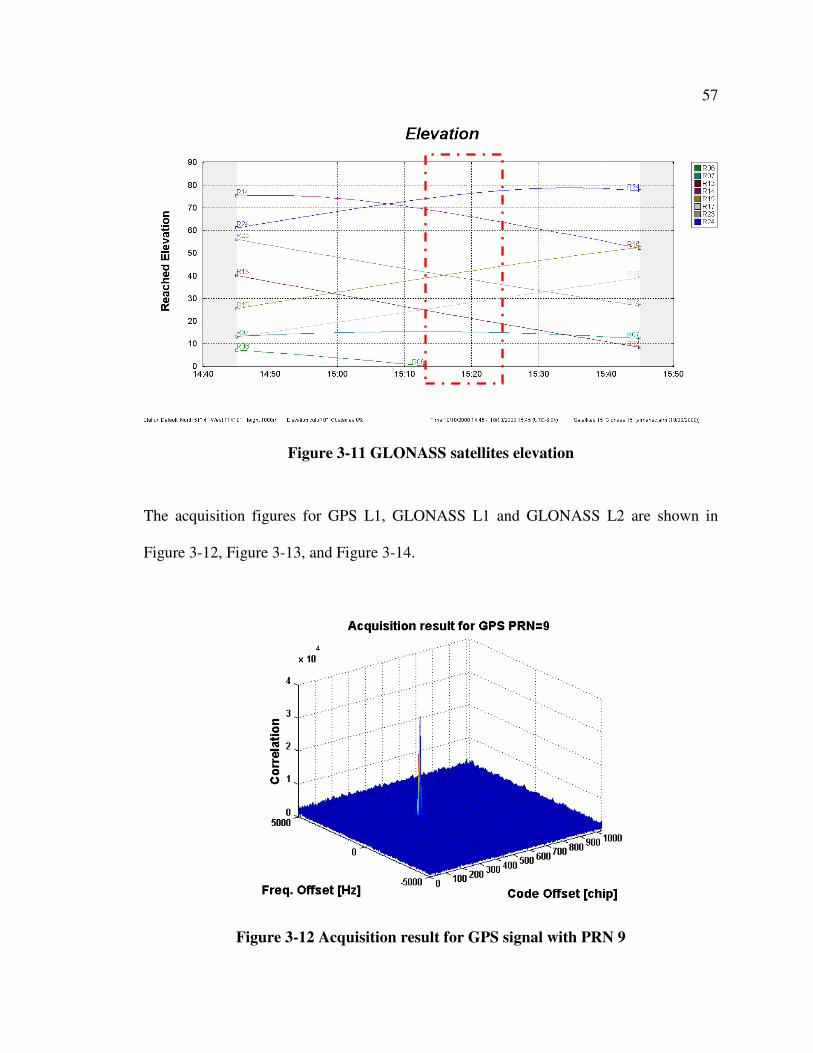
57
Figure 3-11 GLONASS satellites elevation
The acquisition figures for GPS L1, GLONASS L1 and GLONASS L2 are shown in
Figure 3-12, Figure 3-13, and Figure 3-14.
Figure 3-12 Acquisition result for GPS signal with PRN 9

58
Figure 3-13 Acquisition result for GLONASS L1 signal at orbital slot 24
Figure 3-14 Acquisition result for GLONASS L2 signal at orbital slot 24

59
Acquisition results for GLONASS L1 and L2 show that the correlation peak is lower for
GLONASS L2 signal which is related to the power of received L2 signal that is weaker
than L1 signal. However, there are correlation peaks with acceptable power for GPS,
GLONASS L1 and GLONASS L2 which helps in finding the initial value of Doppler
frequency and ranging code offset.
From the acquisition process, code phase offset and Doppler frequency are obtained and
sent to the tracking process. Tracking is discussed in Chapter four. An example of these
values is presented in Table 3-4. These values correspond to the plots above. The code
phase offset for GLONASS L1 and L2 from the same satellite are almost the same. The
ranging code is the same for L1 and L2 signals and these similar values are expected. The
Doppler frequency is proportional to the carrier frequency (Ray 2007), thus the Doppler
frequency for GLONASS L1 and L2 are different.
Table 3-4 Example of acquisition process output
Doppler frequency (HZ) Code offset
(Chips)
GPS PRN 9 825 395.2
GLONASS L1 orbital slot 24 775 2.3
GLONASS L2 orbital slot 24 575 2.3

60
CHAPTER FOUR: TRACKING
4.1 Chapter outline
This Chapter begins with a description of the signal tracking process. Both carrier and
code loops are explained in detail. Phase lock loop, frequency lock loop, and delay lock
loops along with different type of discriminators and loop filters are reviewed. A brief
discussion on tracking loop aiding is presented after that. The Chapter continues with the
introduction of the software which is developed to track GLONASS L1 and L2 signals.
The corresponding modifications to the GPS software receiver are then reviewed. At the
end of the Chapter, some results are presented for the tracked GLONASS L1 and L2
signals.
4.2 Tracking loop overview
The objective of a tracking loop is determining the difference between the locally
generated signal and the incoming pseudo-base-band signal, filtering that estimate and
sending new information to the signal generators. In a tracking loop process, both carrier
and code signals are accurately reproduced inside the receiver. For each carrier and code
portion of the received signal, a tracking loop exists. The code tracking loop is called a
delay lock loop (DLL) and must provide an estimate of code phase of the ranging code
being tracked. The carrier tracking loop is called carrier lock loop (CLL) and it must
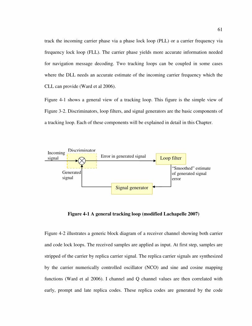
61
track the incoming carrier phase via a phase lock loop (PLL) or a carrier frequency via
frequency lock loop (FLL). The carrier phase yields more accurate information needed
for navigation message decoding. Two tracking loops can be coupled in some cases
where the DLL needs an accurate estimate of the incoming carrier frequency which the
CLL can provide (Ward et al 2006).
Figure 4-1 shows a general view of a tracking loop. This figure is the simple view of
Figure 3-2. Discriminators, loop filters, and signal generators are the basic components of
a tracking loop. Each of these components will be explained in detail in this Chapter.
Figure 4-1 A general tracking loop (modified Lachapelle 2007)
Figure 4-2 illustrates a generic block diagram of a receiver channel showing both carrier
and code lock loops. The received samples are applied as input. At first step, samples are
stripped of the carrier by replica carrier signal. The replica carrier signals are synthesized
by the carrier numerically controlled oscillator (NCO) and sine and cosine mapping
functions (Ward et al 2006). I channel and Q channel values are then correlated with
early, prompt and late replica codes. These replica codes are generated by the code
Loop filter
Signal generator
Discriminator Error in generated signal
“Smoothed” estimate of generated signal error
Generated signal
Incoming signal
62
generator, 2-bit shift register, and the code NCO. In this loop, the code NCO produces
twice the code generator clocking rate (2fco) and sends it to the clock input of the 2-bit
shift register. The code generator clocking rate (fco) is provided by code NCO too. The
2-bit shift register generates two phase-shifted version of the code generated by code
generator (presented by ‘E’ in the diagram). As such, there are three replica codes
designated as early (E), prompt (P), and late (L). If the incoming signal is tracked, the
maximum correlation of the prompt replica code and the incoming signal code is
produced. Under the same circumstance, the correlation of early and late replica codes
with the incoming signal code produces half of the maximum correlation value.
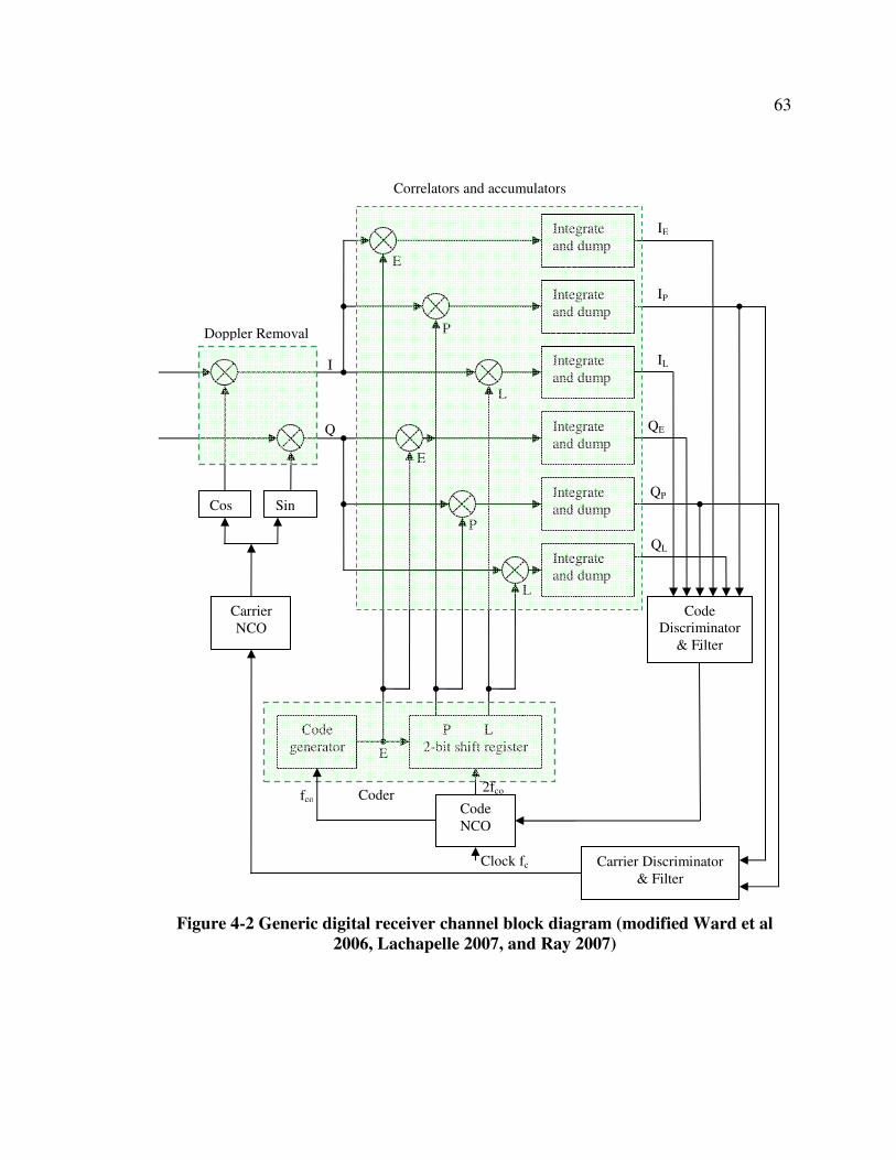
63
Figure 4-2 Generic digital receiver channel block diagram (modified Ward et al
2006, Lachapelle 2007, and Ray 2007)
Integrate
and dump
Integrate
and dump
Integrate
and dump
Sin Cos
Carrier
NCO
Doppler Removal
Code
NCO
Code
generator
P L
2-bit shift register
Integrate
and dump
Integrate
and dump
E
E
P
L
E
P
L
I
Q
Code Discriminator
& Filter
Integrate
and dump
Carrier Discriminator
& Filter
Coder
Correlators and accumulators
IE
IP
IL
QE
QP
QL
Clock fc
fco 2fco
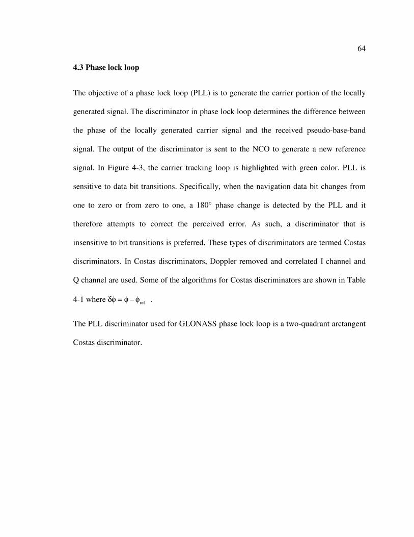
64
4.3 Phase lock loop
The objective of a phase lock loop (PLL) is to generate the carrier portion of the locally
generated signal. The discriminator in phase lock loop determines the difference between
the phase of the locally generated carrier signal and the received pseudo-base-band
signal. The output of the discriminator is sent to the NCO to generate a new reference
signal. In Figure 4-3, the carrier tracking loop is highlighted with green color. PLL is
sensitive to data bit transitions. Specifically, when the navigation data bit changes from
one to zero or from zero to one, a 180° phase change is detected by the PLL and it
therefore attempts to correct the perceived error. As such, a discriminator that is
insensitive to bit transitions is preferred. These types of discriminators are termed Costas
discriminators. In Costas discriminators, Doppler removed and correlated I channel and
Q channel are used. Some of the algorithms for Costas discriminators are shown in Table
4-1 where ref = – δφ φ φ .
The PLL discriminator used for GLONASS phase lock loop is a two-quadrant arctangent
Costas discriminator.

65
Table 4-1 Common Costas loop discriminators (from Ward et al 2006)
Discriminator Output phase error Remarks
Sign(I)×Q
sin( )δφ
• Decision directed Costas
• Near optimal for high SNR
• Least computational burden
I×Q
sin(2 )δφ
• Classic Costas analog discriminator
• Near optimal for low SNR
• Moderate computational burden
Q/I
tan( )δφ
• Suboptimal, but works well for Low and high
SNR
• Higher computational burden
atan(Q/I)
δφ
• Two-quadrant arctangent
• Optimal (Maximum-likelihood estimator) for
both low and high SNR
• Highest computational burden
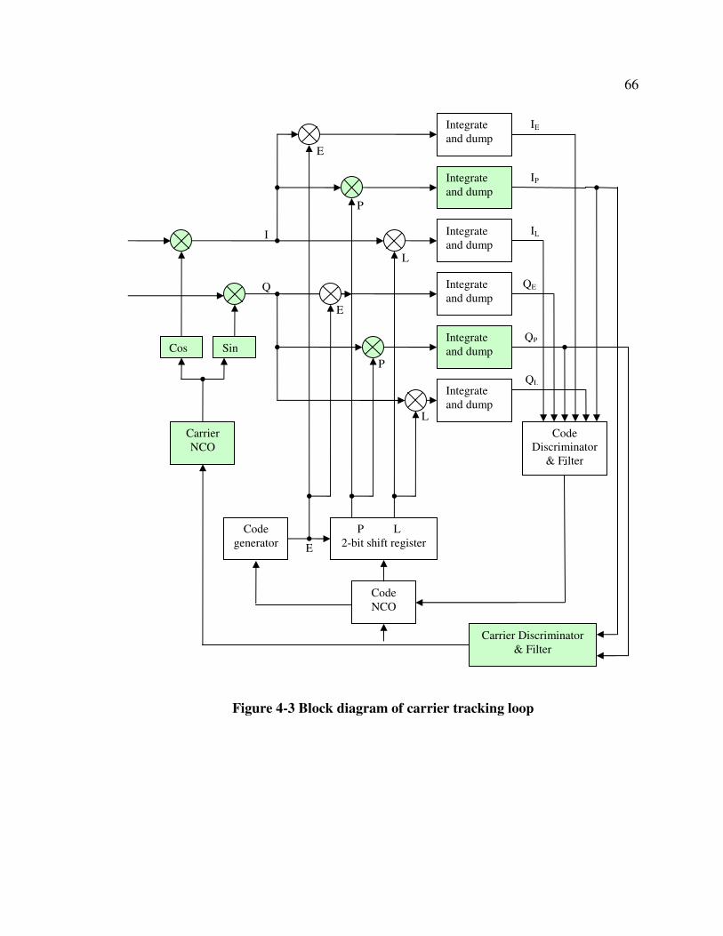
66
Figure 4-3 Block diagram of carrier tracking loop
Integrate
and dump
Integrate
and dump
Integrate
and dump
Sin Cos
Carrier
NCO
Code
NCO
Code
generator
P L
2-bit shift register
Integrate
and dump
Integrate
and dump
E
E
P
L
E
P
L
I
Q
Code Discriminator
& Filter
Integrate
and dump
Carrier Discriminator
& Filter
IE
IP
IL
QE
QP
QL
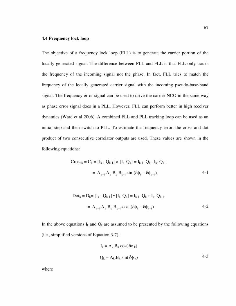
67
4.4 Frequency lock loop
The objective of a frequency lock loop (FLL) is to generate the carrier portion of the
locally generated signal. The difference between PLL and FLL is that FLL only tracks
the frequency of the incoming signal not the phase. In fact, FLL tries to match the
frequency of the locally generated carrier signal with the incoming pseudo-base-band
signal. The frequency error signal can be used to drive the carrier NCO in the same way
as phase error signal does in a PLL. However, FLL can perform better in high receiver
dynamics (Ward et al 2006). A combined FLL and PLL tracking loop can be used as an
initial step and then switch to PLL. To estimate the frequency error, the cross and dot
product of two consecutive correlator outputs are used. These values are shown in the
following equations:
Crossk = Ck = [Ik-1 Qk-1] × [Ik Qk] = Ik-1. Qk - Ik. Qk-1
= k 1 k k k 1 k k 1A .A .B .B .sin ( )− − −δφ − δφ
4-1
Dotk = Dk= [Ik-1 Qk-1] • [Ik Qk] = Ik-1. Qk + Ik. Qk-1.
= k 1 k k k 1 k k 1A .A .B .B .cos ( )− − −δφ − δφ
4-2
In the above equations Ik and Qk are assumed to be presented by the following equations
(i.e., simplified versions of Equation 3-7):
Ik = Ak.Bk.cos( δφ k)
Qk = Ak.Bk.sin( δφ k)
4-3
where
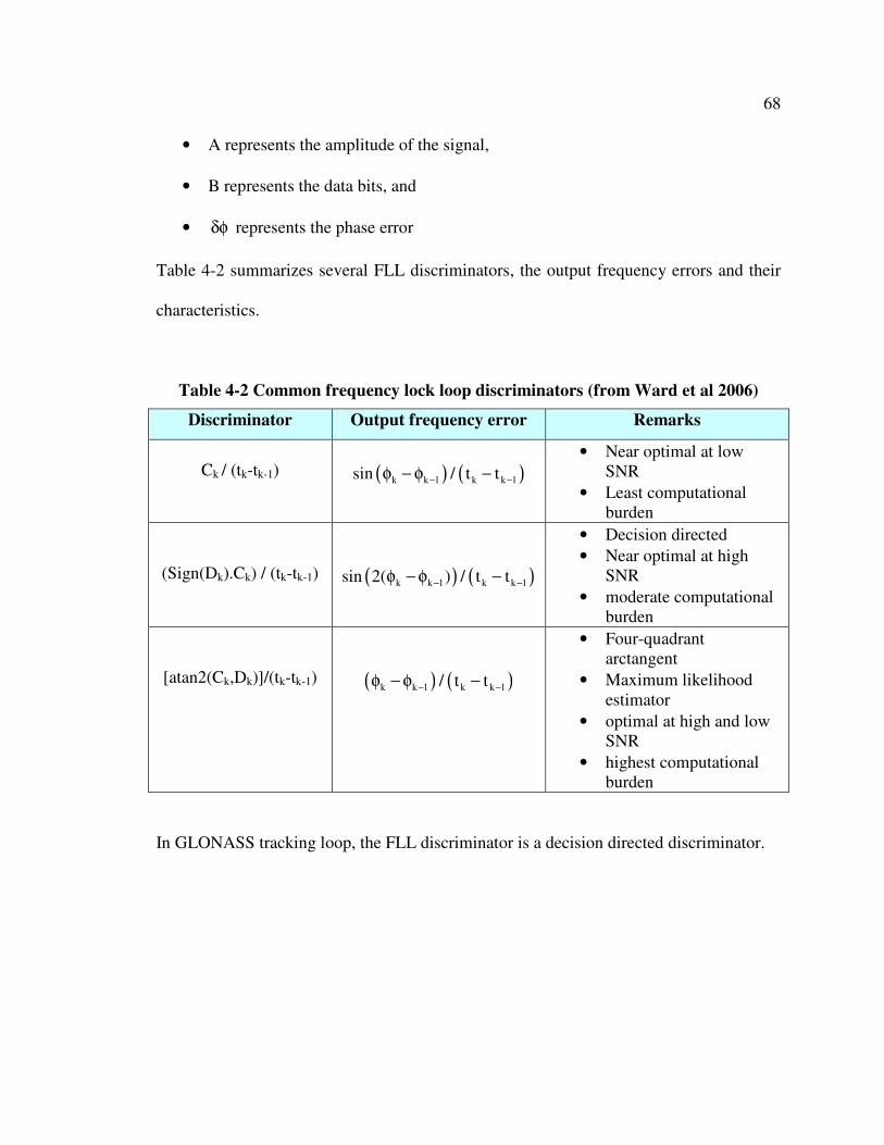
68
• A represents the amplitude of the signal,
• B represents the data bits, and
• δφ represents the phase error
Table 4-2 summarizes several FLL discriminators, the output frequency errors and their
characteristics.
Table 4-2 Common frequency lock loop discriminators (from Ward et al 2006)
Discriminator Output frequency error Remarks
Ck / (tk-tk-1)
( ) ( )k k 1 k k 1sin / t t− −φ − φ −
• Near optimal at low SNR
• Least computational burden
(Sign(Dk).Ck) / (tk-tk-1)
( ) ( )k k 1 k k 1sin 2( ) / t t− −φ − φ −
• Decision directed
• Near optimal at high SNR
• moderate computational burden
[atan2(Ck,Dk)]/(tk-tk-1)
( ) ( )k k 1 k k 1/ t t− −φ − φ −
• Four-quadrant arctangent
• Maximum likelihood estimator
• optimal at high and low SNR
• highest computational burden
In GLONASS tracking loop, the FLL discriminator is a decision directed discriminator.
69
4.5 Delay lock loop
The objective of a delay lock loop (DLL) is to track the standard ranging code of the
received pseudo-base-band signal by generating a local standard ranging code. This loop
consists of correlator, accumulator, DLL discriminator and loop filter as is shown in
Figure 4-4 in yellow color. The inputs to the DLL are Doppler removed samples
modulated with navigation data and ranging code. To remove this ranging code, it is
required to generate three pairs of I and Q values; early (IE, QE), prompt or punctual (IP,
QP), and late (IL, QL), where E, P, and L subscripts stand for early, punctual and late
respectively. Early and late values are typically one chip away from each other and are
half chip spaced from the prompt value (Ward et al 2007).
There are two types of DLL discriminators:
1. Coherent discriminator: where all power is on I channel, implying phase lock is
achieved.
2. Non-coherent discriminator: where phase lock is not required.
Some types of DLL discriminators are presented in Table 4-3. In this table E and L
represent the following equations:
2 2
E EE = I + Q
2 2
L LL = I + Q
4-4
4-5
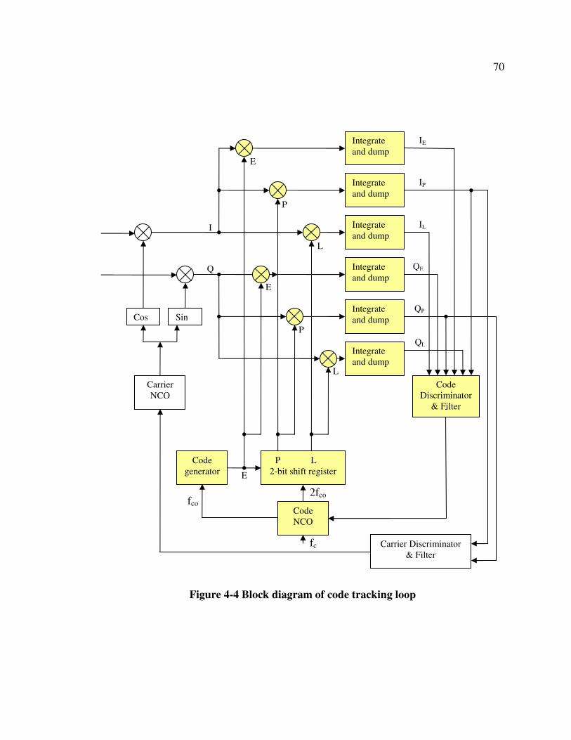
70
Figure 4-4 Block diagram of code tracking loop
Integrate
and dump
Integrate
and dump
Integrate
and dump
Sin Cos
Carrier
NCO
Code
NCO
Code
generator
P L
2-bit shift register
Integrate
and dump
Integrate
and dump
E
E
P
L
E
P
L
I
Q
Code Discriminator
& Filter
Integrate
and dump
Carrier Discriminator
& Filter
IE
IP
IL
QE
QP
QL
fc
fco 2fco
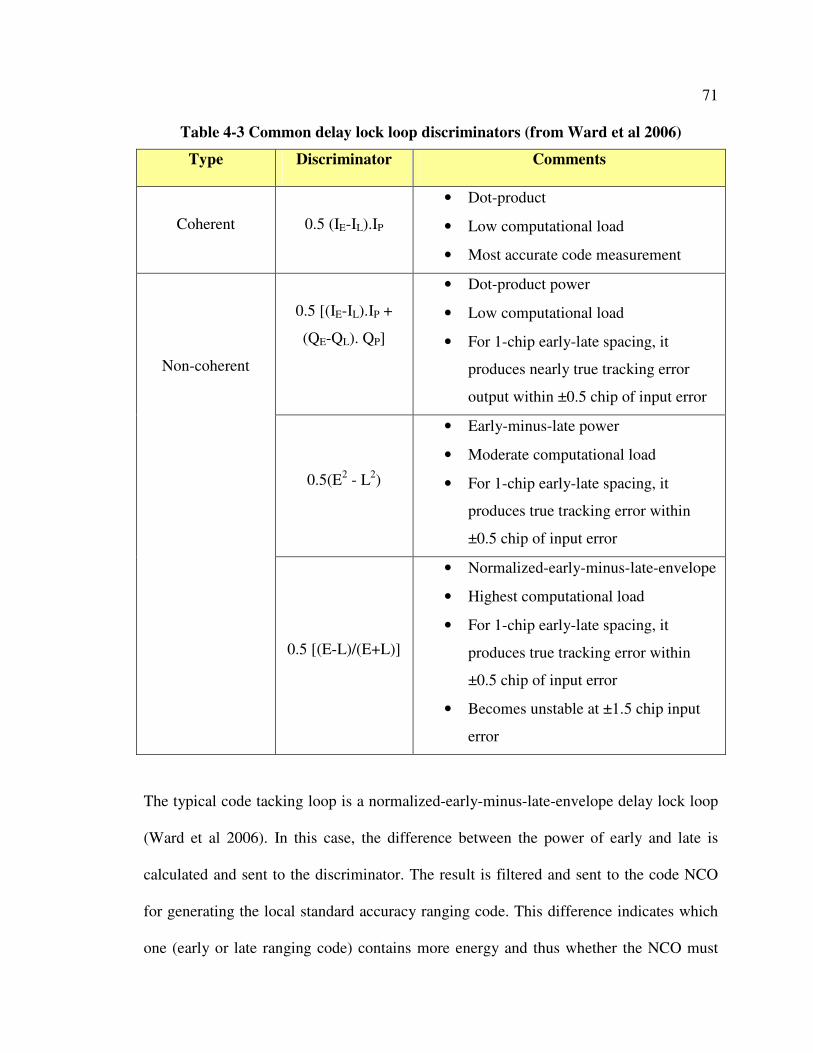
71
Table 4-3 Common delay lock loop discriminators (from Ward et al 2006)
Type Discriminator Comments
Coherent
0.5 (IE-IL).IP
• Dot-product
• Low computational load
• Most accurate code measurement
0.5 [(IE-IL).IP +
(QE-QL). QP]
• Dot-product power
• Low computational load
• For 1-chip early-late spacing, it
produces nearly true tracking error
output within ±0.5 chip of input error
0.5(E2 - L2)
• Early-minus-late power
• Moderate computational load
• For 1-chip early-late spacing, it
produces true tracking error within
±0.5 chip of input error
Non-coherent
0.5 [(E-L)/(E+L)]
• Normalized-early-minus-late-envelope
• Highest computational load
• For 1-chip early-late spacing, it
produces true tracking error within
±0.5 chip of input error
• Becomes unstable at ±1.5 chip input
error
The typical code tacking loop is a normalized-early-minus-late-envelope delay lock loop
(Ward et al 2006). In this case, the difference between the power of early and late is
calculated and sent to the discriminator. The result is filtered and sent to the code NCO
for generating the local standard accuracy ranging code. This difference indicates which
one (early or late ranging code) contains more energy and thus whether the NCO must
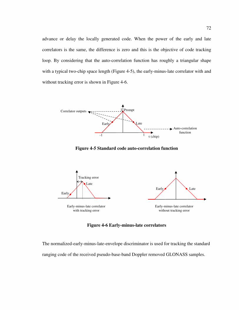
72
advance or delay the locally generated code. When the power of the early and late
correlators is the same, the difference is zero and this is the objective of code tracking
loop. By considering that the auto-correlation function has roughly a triangular shape
with a typical two-chip space length (Figure 4-5), the early-minus-late correlator with and
without tracking error is shown in Figure 4-6.
Figure 4-5 Standard code auto-correlation function
Figure 4-6 Early-minus-late correlators
The normalized-early-minus-late-envelope discriminator is used for tracking the standard
ranging code of the received pseudo-base-band Doppler removed GLONASS samples.
Late
Early
Early Late
Tracking error
Early-minus-late correlator with tracking error
Early-minus-late correlator without tracking error
τ (chip) 1-1
1
Early Late
Prompt
Auto-correlation function
Correlator outputs
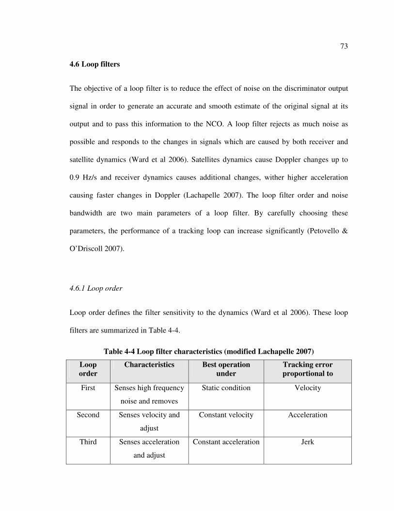
73
4.6 Loop filters
The objective of a loop filter is to reduce the effect of noise on the discriminator output
signal in order to generate an accurate and smooth estimate of the original signal at its
output and to pass this information to the NCO. A loop filter rejects as much noise as
possible and responds to the changes in signals which are caused by both receiver and
satellite dynamics (Ward et al 2006). Satellites dynamics cause Doppler changes up to
0.9 Hz/s and receiver dynamics causes additional changes, wither higher acceleration
causing faster changes in Doppler (Lachapelle 2007). The loop filter order and noise
bandwidth are two main parameters of a loop filter. By carefully choosing these
parameters, the performance of a tracking loop can increase significantly (Petovello &
O’Driscoll 2007).
4.6.1 Loop order
Loop order defines the filter sensitivity to the dynamics (Ward et al 2006). These loop
filters are summarized in Table 4-4.
Table 4-4 Loop filter characteristics (modified Lachapelle 2007)
Loop
order
Characteristics Best operation
under
Tracking error
proportional to
First Senses high frequency
noise and removes
Static condition Velocity
Second Senses velocity and
adjust
Constant velocity Acceleration
Third Senses acceleration
and adjust
Constant acceleration Jerk
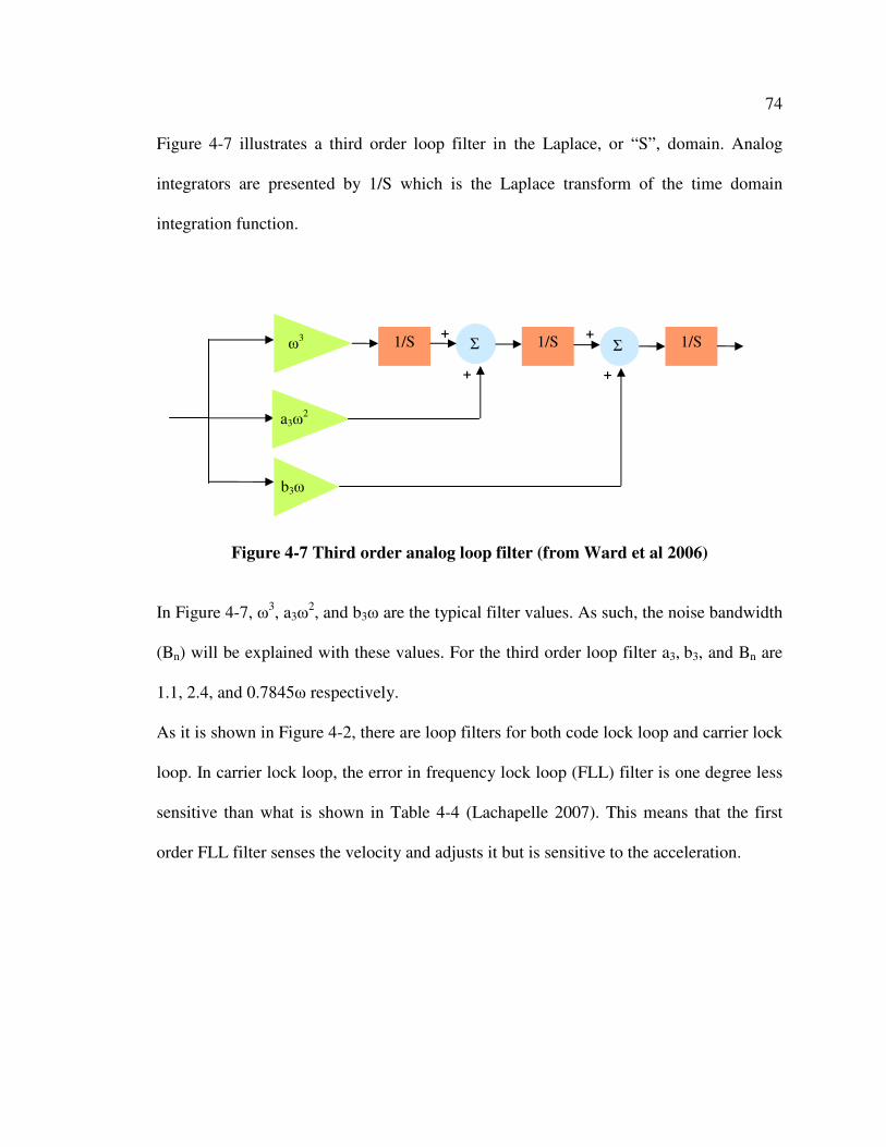
74
Figure 4-7 illustrates a third order loop filter in the Laplace, or “S”, domain. Analog
integrators are presented by 1/S which is the Laplace transform of the time domain
integration function.
Figure 4-7 Third order analog loop filter (from Ward et al 2006)
In Figure 4-7, ω3, a3ω2, and b3ω are the typical filter values. As such, the noise bandwidth
(Bn) will be explained with these values. For the third order loop filter a3, b3, and Bn are
1.1, 2.4, and 0.7845ω respectively.
As it is shown in Figure 4-2, there are loop filters for both code lock loop and carrier lock
loop. In carrier lock loop, the error in frequency lock loop (FLL) filter is one degree less
sensitive than what is shown in Table 4-4 (Lachapelle 2007). This means that the first
order FLL filter senses the velocity and adjusts it but is sensitive to the acceleration.
a3ω2
ω3
b3ω
1/S Σ 1/S Σ 1/S
+
+
+
+
75
4.6.2 Loop bandwidth
The loop bandwidth must be set in a way that rejects as mush noise as possible. On the
other hand, it must be wide enough to contain both satellite and receiver dynamics. For
example, when the receiver is in static condition, the Doppler shift is approximately ±5
kHz, but for moving receiver it can be ±10 kHz or more (Lachapelle 2007). As such, the
bandwidth must be sufficiently wide to pass true signal dynamics unchanged.
4.7 Tracking loop aiding
As discussed above, the loop bandwidth must be sufficiently wide to let actual signal
dynamics pass and also be sufficiently narrow to prevent the noise to pass. Thus, there is
always a compromise between having more noise and true signals. On the other hand, in
some cases, the signal dynamics can be measured externally and removed. Then, the
noise bandwidth can be reduced. This is the concept of tracking loop aiding. Figure 4-8
illustrates the block diagram of the code tacking loop aiding with carrier tracking loop.
The carrier tracking loop is adjusted by a scale factor, then the code loop filter output is
added to it. The result is sent to the code NCO. The scale factor is presented as the
following equation (Ward et al 2006):
Scale factor = c
L
R
f
4-6
where
• Rc represents code chip rate (Hz) plus C/A code Doppler effect, and
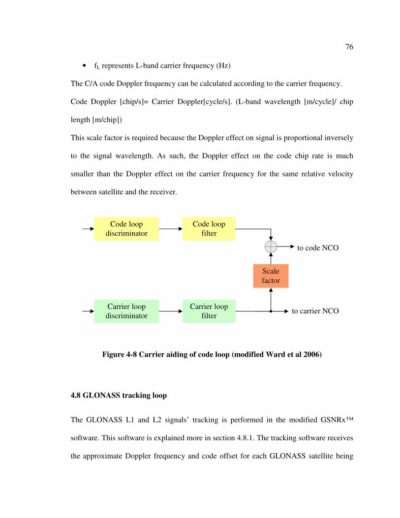
76
• fL represents L-band carrier frequency (Hz)
The C/A code Doppler frequency can be calculated according to the carrier frequency.
Code Doppler [chip/s]= Carrier Doppler[cycle/s]. (L-band wavelength [m/cycle]/ chip
length [m/chip])
This scale factor is required because the Doppler effect on signal is proportional inversely
to the signal wavelength. As such, the Doppler effect on the code chip rate is much
smaller than the Doppler effect on the carrier frequency for the same relative velocity
between satellite and the receiver.
Figure 4-8 Carrier aiding of code loop (modified Ward et al 2006)
4.8 GLONASS tracking loop
The GLONASS L1 and L2 signals’ tracking is performed in the modified GSNRx™
software. This software is explained more in section 4.8.1. The tracking software receives
the approximate Doppler frequency and code offset for each GLONASS satellite being
Code loop
discriminator
Code loop
filter
Carrier loop
discriminator
Carrier loop
filter
Scale
factor
to code NCO
to carrier NCO

77
acquired from the acquisition process explained in Chapter three. The tracking software
uses these parameters to generate some measurements which can be used to generate a
navigation solution.
4.8.1 GSNRx™
GNSS Software Navigation Receiver (GSNRx™) is a C++ class-based GNSS software
receiver program developed in Position, Location And Navigation (PLAN) group at the
University of Calgary (Petovello et al 2008). This software is basically developed for
GPS L1 C/A signal and is capable of processing the raw samples from the RF front-end
and generating measurements to be used in other data processing programs. Also, it can
produce navigation solution in post-mission. GSNRx™ is used as the basis for tracking
GLONASS L1 and L2 signals. A general view of this software receiver is shown in
Figure 4-9.
The software is initialized using an option file in which different parameters can be set by
the user. The fields of the option file that are relevant to this research are explained in
section 4.8.2.
As part of this research, the GSNRx™ software was modified to allow tracking of the
GLONASS L1 and L2 signals for as many GLONASS satellites as possible.

78
Figure 4-9 Block diagram of GSNRx™ (from Petovello & O’Driscoll 2007)
Load option file and initialize the receiver
Read 1 ms of data
End of file?
Exit
Process tracking channel
Process acquisition
channel
Update channel
list
Start
Samples
remaining
Doppler removal &
correlation
Code rollover?
Bit Synch Nav decode
Track status
Time for
loop update Loop update
Exit No Yes
No
No Yes
Yes
79
In GSNRx™ tracking, the received samples are first shifted to baseband (using Doppler
removal) and correlated with the local code. Then, on each code rollover event, bit
synchronization, navigation message decoding and tracking status updates are performed
for each channel (Figure 4-9). Code rollover is an event specific to each tracking channel.
The outputs of the Doppler removal and correlation are accumulated and when the
accumulation period and tracking loop update periods are equal, the tracking loops are
updated (Petovello & O’Driscoll 2007). For GLONASS tracking process, the Doppler
removal and correlation component needs some modification. Different locally generated
frequencies as discussed in section 3.6.2 are needed for each GLONASS satellite.
Moreover, the locally generated ranging code for correlation must be in the format
discussed in section 3.6.1. Considering the effect of meander code, the bit
synchronization for GLONASS is different from GPS which is discussed in Chapter five.
Also, the GLONASS navigation message needs its specific navigation message decoding
algorithm which is explained in Chapter five.
4.8.2 Option file
The details of the relevant options for GLONASS (relative to GPS) are explained below.
The values illustrated are for GLONASS L1 and L2 signals unless stated otherwise.
• Data file: This field contains the name of the raw data file. This file includes a
stream of bytes. Each byte represents a sample from the RF front-end. GLONASS
L1 and L2 feed two different raw files to the option file because of their different
carrier frequencies.
80
• Intermediate frequency: This field represents the intermediate frequency of the
samples in the file presented in data file field. This value is set 4 MHz.
• Sampling rate: this filed represent the sampling rate of the samples in the file
presented in data file field. This value is set 12.5 MSps.
• Maximum coherent integration: This field represents the maximum length of the
coherent integration in a channel. This value is set 10 ms for GLONASS because
the received GLONASS navigation data bit is 10 ms.
• Type of carrier loop: The carrier loop can operate in PLL or FLL-assisted PLL
mode. For GLONASS tracking loop, PLL is chosen.
• PLL bandwidth: As discussed in section 4.8, the loop bandwidth can be fixed or
variable. This field is a space to change the bandwidth of the PLL. For
GLONASS, the bandwidth of PLL is set 15 Hz.
• FLL bandwidth: In this field the bandwidth of FLL can be set. The bandwidth of
FLL is set 8 Hz for GLONASS.
• Initial DLL bandwidth: In this field DLL bandwidth is set before the aiding with
carrier lock loop. This value is set 2 Hz for GLONASS.
• Assisted DLL bandwidth: This field define the DLL bandwidth after aiding with
carrier lock loop. This value is set 0.05 Hz for GLONASS.
• PRN: It indicates the satellite number which is going to be tracked. For
GLONASS, this filed represents the satellites being acquired and are ready to be
tracked. This field must be followed by approximate Doppler frequency (Hz) and
81
code phase (Chips) which are acquired in acquisition process discussed in Chapter
three.
• Doppler: As explained above, this field indicates the Doppler frequency (Hz) of
the satellite being acquired and is passed to this option file for tracking.
• Code phase: This field is dedicated to the code phase (Chips) of the satellite being
acquired and is passed to this option file for tracking. It must follow the PRN and
Doppler fields.
4.8.3 Tracking loop implementation in GSNRx™
The mode of the tracking loop can be reflected by a parameter called tracking state for
each channel. The software uses two indicators called frequency lock indicator (FLI) and
phase lock indicator (PLI) for the transition between tracking states. FLI (Mongredien et
al 2006) and PLI (Van Dierendonck 1995) are defined by the following equations:
2 2
k k
2 2k
k k
D - CFLI =
D + C = cos(4πδfkTcoh)
4-7
( )2 2
k kk k2 2
k k
I - QPLI cos 2
I Q= = δφ
+
4-8
Dk and Ck are explained in section 4.4 and Tcoh is the coherent integration time.
According to the equations 4-7 and 4-8, FLI and PLI range between minus one in the
worse case and positive one in the best case.
Tracking states and a short description for each state is summarized in Table 4-5. To
achieve phase lock loop which is the ultimate goal of a tracking loop, it is required to

82
achieve frequency lock loop at first to avoid false lock in PLL. On the other hand, loss of
lock must be detected. By comparing the FLI and PLI values against different thresholds
(that depend on the current tracking state), the software is able to successfully track
signals in a robust manner.
Table 4-5 Tracking states summary
Tracking state Description
Initialization
• Carrier tracking loop is performed using FLL alone
• Gives time to FLI to converge before being used for
decision making
Wideband FLL
• Carrier tracking loop is performed using FLL alone
• A constant 1-ms integration time is used to maintain ±250
Hz pull-in range
Narrowband FLL • Carrier tracking loop is performed using FLL alone
• Integration time is maximized for fine frequency tracking
FLL-assisted PLL • Carrier tracking loop is performed using FLL-assisted PLL
• DLL aiding with CLL begins
PLL • Carrier tracking loop is performed using PLL
4.9 Tracking Results
In this section, the tracking results for GLONASS L1 and L2 signals are presented beside
the tracking status. The tracking statuses are defined by numbers in the tracking software
as shown in Table 4-6. Presenting tracking status besides each result helps to more easily
explain the result obtained.
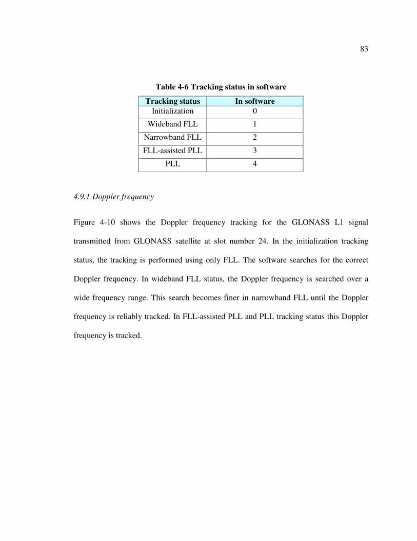
83
Table 4-6 Tracking status in software
Tracking status In software
Initialization 0
Wideband FLL 1
Narrowband FLL 2
FLL-assisted PLL 3
PLL 4
4.9.1 Doppler frequency
Figure 4-10 shows the Doppler frequency tracking for the GLONASS L1 signal
transmitted from GLONASS satellite at slot number 24. In the initialization tracking
status, the tracking is performed using only FLL. The software searches for the correct
Doppler frequency. In wideband FLL status, the Doppler frequency is searched over a
wide frequency range. This search becomes finer in narrowband FLL until the Doppler
frequency is reliably tracked. In FLL-assisted PLL and PLL tracking status this Doppler
frequency is tracked.
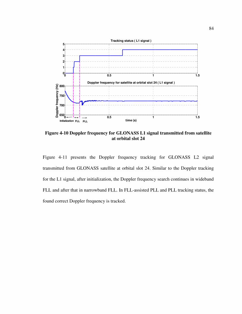
84
0 0.5 1 1.50
1
2
3
4
5Tracking status ( L1 signal )
0 0.5 1 1.5650
700
750
800Doppler frequency for satellite at orbital slot 24 ( L1 signal )
Do
pp
ler
freq
uen
cy (
Hz)
time (s)PLLFLLInitialization
Figure 4-10 Doppler frequency for GLONASS L1 signal transmitted from satellite
at orbital slot 24
Figure 4-11 presents the Doppler frequency tracking for GLONASS L2 signal
transmitted from GLONASS satellite at orbital slot 24. Similar to the Doppler tracking
for the L1 signal, after initialization, the Doppler frequency search continues in wideband
FLL and after that in narrowband FLL. In FLL-assisted PLL and PLL tracking status, the
found correct Doppler frequency is tracked.
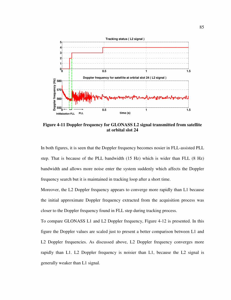
85
0 0.5 1 1.50
1
2
3
4
5Tracking status ( L2 signal )
0 0.5 1 1.5550
560
570
580Doppler frequency for satellite at orbital slot 24 ( L2 signal )
Do
pp
ler
freq
uen
cy (
Hz)
time (s)PLLFLLInitilaization
Figure 4-11 Doppler frequency for GLONASS L2 signal transmitted from satellite
at orbital slot 24
In both figures, it is seen that the Doppler frequency becomes nosier in FLL-assisted PLL
step. That is because of the PLL bandwidth (15 Hz) which is wider than FLL (8 Hz)
bandwidth and allows more noise enter the system suddenly which affects the Doppler
frequency search but it is maintained in tracking loop after a short time.
Moreover, the L2 Doppler frequency appears to converge more rapidly than L1 because
the initial approximate Doppler frequency extracted from the acquisition process was
closer to the Doppler frequency found in FLL step during tracking process.
To compare GLONASS L1 and L2 Doppler frequency, Figure 4-12 is presented. In this
figure the Doppler values are scaled just to present a better comparison between L1 and
L2 Doppler frequencies. As discussed above, L2 Doppler frequency converges more
rapidly than L1. L2 Doppler frequency is noisier than L1, because the L2 signal is
generally weaker than L1 signal.
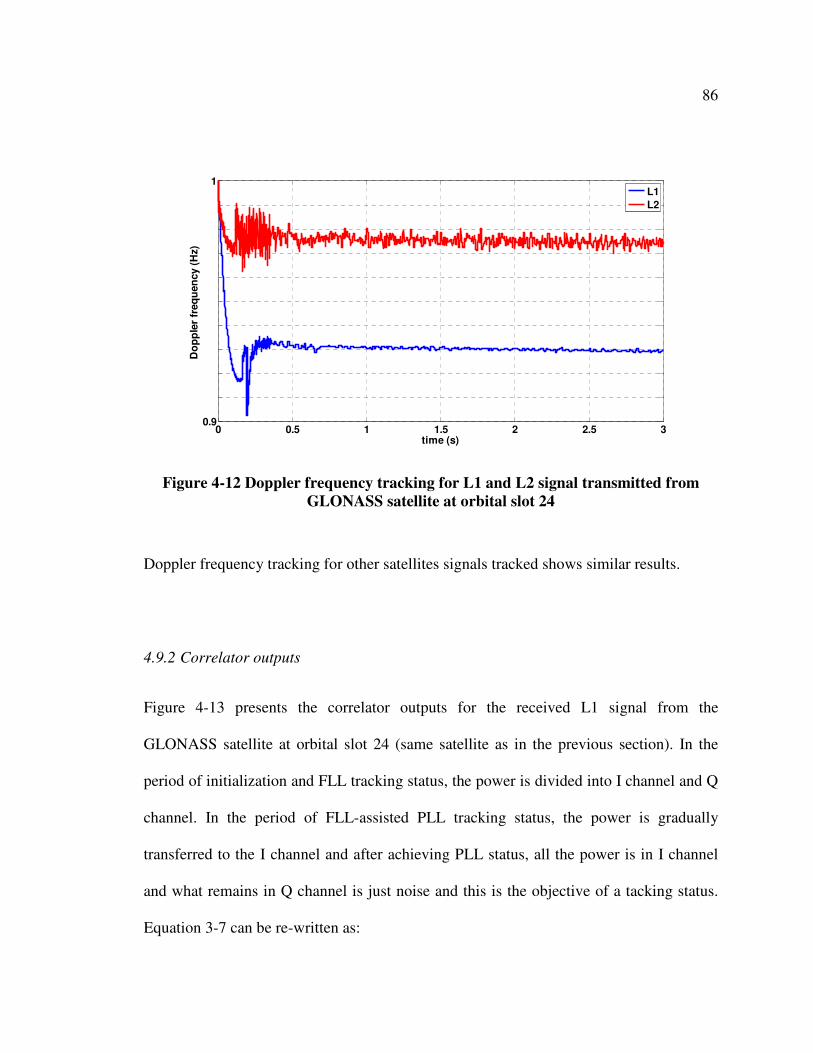
86
0 0.5 1 1.5 2 2.5 30.9
1
time (s)
Do
pp
ler
freq
uen
cy (
Hz)
L1
L2
Figure 4-12 Doppler frequency tracking for L1 and L2 signal transmitted from
GLONASS satellite at orbital slot 24
Doppler frequency tracking for other satellites signals tracked shows similar results.
4.9.2 Correlator outputs
Figure 4-13 presents the correlator outputs for the received L1 signal from the
GLONASS satellite at orbital slot 24 (same satellite as in the previous section). In the
period of initialization and FLL tracking status, the power is divided into I channel and Q
channel. In the period of FLL-assisted PLL tracking status, the power is gradually
transferred to the I channel and after achieving PLL status, all the power is in I channel
and what remains in Q channel is just noise and this is the objective of a tacking status.
Equation 3-7 can be re-written as:
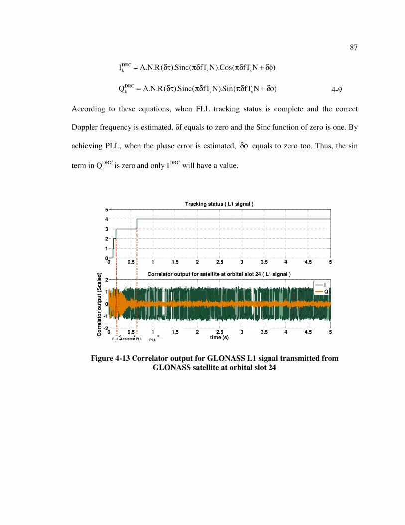
87
DRC
k s s
DRC
k s s
I A.N.R( ).Sinc( fT N).Cos( fT N )
Q A.N.R( ).Sinc( fT N).Sin( fT N )
= δτ πδ πδ + δφ
= δτ πδ πδ + δφ
4-9
According to these equations, when FLL tracking status is complete and the correct
Doppler frequency is estimated, δf equals to zero and the Sinc function of zero is one. By
achieving PLL, when the phase error is estimated, δφ equals to zero too. Thus, the sin
term in QDRC is zero and only IDRC will have a value.
0 0.5 1 1.5 2 2.5 3 3.5 4 4.5 50
1
2
3
4
5Tracking status ( L1 signal )
0 0.5 1 1.5 2 2.5 3 3.5 4 4.5 5-2
-1
0
1
2
time (s)
Co
rrela
tor
ou
tpu
t (S
cale
d) Correlator output for satellite at orbital slot 24 ( L1 signal )
I
Q
PLLFLL-Assisted PLL
Figure 4-13 Correlator output for GLONASS L1 signal transmitted from
GLONASS satellite at orbital slot 24
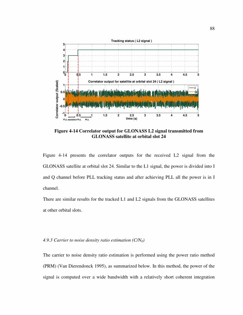
88
0 0.5 1 1.5 2 2.5 3 3.5 4 4.5 50
1
2
3
4
5Tracking status ( L2 signal )
0 0.5 1 1.5 2 2.5 3 3.5 4 4.5 5-1
-0.5
0
0.5
1
time (s)Co
rrela
tor
ou
tpu
t (S
cale
d) Correlator output for satellite at orbital slot 24 ( L2 signal )
I
Q
PLLFLL-assisted PLL
Figure 4-14 Correlator output for GLONASS L2 signal transmitted from
GLONASS satellite at orbital slot 24
Figure 4-14 presents the correlator outputs for the received L2 signal from the
GLONASS satellite at orbital slot 24. Similar to the L1 signal, the power is divided into I
and Q channel before PLL tracking status and after achieving PLL all the power is in I
channel.
There are similar results for the tracked L1 and L2 signals from the GLONASS satellites
at other orbital slots.
4.9.3 Carrier to noise density ratio estimation (C/N0)
The carrier to noise density ratio estimation is performed using the power ratio method
(PRM) (Van Dierendonck 1995), as summarized below. In this method, the power of the
signal is computed over a wide bandwidth with a relatively short coherent integration
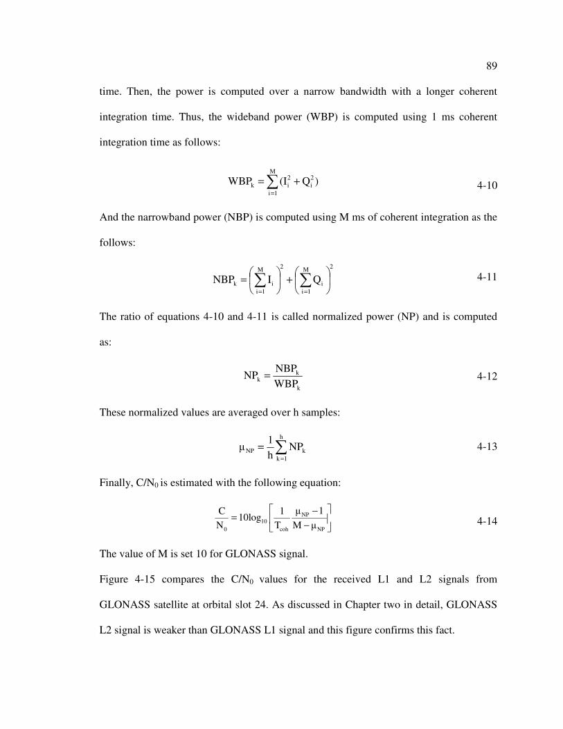
89
time. Then, the power is computed over a narrow bandwidth with a longer coherent
integration time. Thus, the wideband power (WBP) is computed using 1 ms coherent
integration time as follows:
∑=
+=M
1i
2
i
2
ik )Q(IWBP
4-10
And the narrowband power (NBP) is computed using M ms of coherent integration as the
follows:
2M
1i
i
2M
1i
ik QINBP
+
= ∑∑
==
4-11
The ratio of equations 4-10 and 4-11 is called normalized power (NP) and is computed
as:
k
kk
WBP
NBPNP =
4-12
These normalized values are averaged over h samples:
∑=
=h
1k
kNP NPh
1µ
4-13
Finally, C/N0 is estimated with the following equation:
NP10
0 coh NP
µ 1C 110log
N T M µ
−=
−
4-14
The value of M is set 10 for GLONASS signal.
Figure 4-15 compares the C/N0 values for the received L1 and L2 signals from
GLONASS satellite at orbital slot 24. As discussed in Chapter two in detail, GLONASS
L2 signal is weaker than GLONASS L1 signal and this figure confirms this fact.

90
0 0.5 1 1.5 2 2.5 3 3.5 4 4.5 525
30
35
40
45
50
55
60
time (s)
C/N
0(d
B-H
z)
C/N0 for satellite at orbital slot 24
L1
L2
Figure 4-15 C/N0 estimation for GLONASS L1 and L2 signal transmitted from
GLONASS satellite at orbital slot 24
Table 4-7 summarizes the C/N0 values for L1 and L2 signals being tracked. The values in
the table represent average C/N0 values over ten minutes. This table shows that the L2
C/N0 values are lower than L1 values from the same satellite. The differences between L1
and L2 C/N0 value are around 3 dB-Hz for all the satellites except for satellite at orbital
slot 24. L1 signal received from GLONASS satellite at orbital slot 24 is strong.
Figure 4-16 presents the C/N0 values for all the GLONASS L1 and L2 signals. This
figure plus Table 4-7 confirm that L2 signal received from GLONASS satellite at orbital
slot 23 is so weak (with average value of 35 dB-Hz over ten minutes) and the L1 signal
received from GLONASS satellite at orbital slot 24 is the strongest signal.
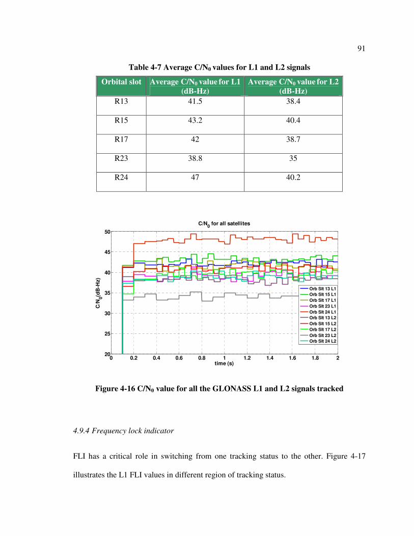
91
Table 4-7 Average C/N0 values for L1 and L2 signals
Orbital slot Average C/N0 value for L1
(dB-Hz)
Average C/N0 value for L2
(dB-Hz)
R13 41.5 38.4
R15 43.2 40.4
R17 42 38.7
R23 38.8 35
R24 47 40.2
0 0.2 0.4 0.6 0.8 1 1.2 1.4 1.6 1.8 220
25
30
35
40
45
50
time (s)
C/N
0(d
B-H
z)
C/N0 for all satellites
Orb Slt 13 L1
Orb Slt 15 L1
Orb Slt 17 L1
Orb Slt 23 L1
Orb Slt 24 L1
Orb Slt 13 L2
Orb Slt 15 L2
Orb Slt 17 L2
Orb Slt 23 L2
Orb Slt 24 L2
Figure 4-16 C/N0 value for all the GLONASS L1 and L2 signals tracked
4.9.4 Frequency lock indicator
FLI has a critical role in switching from one tracking status to the other. Figure 4-17
illustrates the L1 FLI values in different region of tracking status.
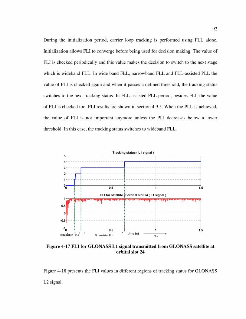
92
During the initialization period, carrier loop tracking is performed using FLL alone.
Initialization allows FLI to converge before being used for decision making. The value of
FLI is checked periodically and this value makes the decision to switch to the next stage
which is wideband FLL. In wide band FLL, narrowband FLL and FLL-assisted PLL the
value of FLI is checked again and when it passes a defined threshold, the tracking status
switches to the next tracking status. In FLL-assisted PLL period, besides FLI, the value
of PLI is checked too. PLI results are shown in section 4.9.5. When the PLL is achieved,
the value of FLI is not important anymore unless the PLI decreases below a lower
threshold. In this case, the tracking status switches to wideband FLL.
0 0.5 1 1.50
1
2
3
4
5Tracking status ( L1 signal )
0 0.5 1 1.5-1
-0.5
0
0.5
1FLI for satellite at orbital slot 24 ( L1 signal )
time (s)FLL-assisted PLLFLL PLLInitialization
Figure 4-17 FLI for GLONASS L1 signal transmitted from GLONASS satellite at
orbital slot 24
Figure 4-18 presents the FLI values in different regions of tracking status for GLONASS
L2 signal.
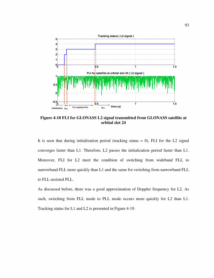
93
0 0.5 1 1.50
1
2
3
4
5Tracking status ( L2 signal )
0 0.5 1 1.5-0.5
0
0.5
1FLI for satellite at orbital slot 24 ( L2 signal )
time (s)FLL-assisted PLL PLLFLLInitialization
Figure 4-18 FLI for GLONASS L2 signal transmitted from GLONASS satellite at
orbital slot 24
It is seen that during initialization period (tracking status = 0), FLI for the L2 signal
converges faster than L1. Therefore, L2 passes the initialization period faster than L1.
Moreover, FLI for L2 meet the condition of switching from wideband FLL to
narrowband FLL more quickly than L1 and the same for switching from narrowband FLL
to FLL-assisted PLL.
As discussed before, there was a good approximation of Doppler frequency for L2. As
such, switching from FLL mode to PLL mode occurs more quickly for L2 than L1.
Tracking status for L1 and L2 is presented in Figure 4-19.
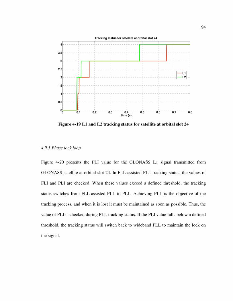
94
0 0.1 0.2 0.3 0.4 0.5 0.6 0.7 0.80
0.5
1
1.5
2
2.5
3
3.5
4
time (s)
Tracking status for satellite at orbital slot 24
L1
L2
Figure 4-19 L1 and L2 tracking status for satellite at orbital slot 24
4.9.5 Phase lock loop
Figure 4-20 presents the PLI value for the GLONASS L1 signal transmitted from
GLONASS satellite at orbital slot 24. In FLL-assisted PLL tracking status, the values of
FLI and PLI are checked. When these values exceed a defined threshold, the tracking
status switches from FLL-assisted PLL to PLL. Achieving PLL is the objective of the
tracking process, and when it is lost it must be maintained as soon as possible. Thus, the
value of PLI is checked during PLL tracking status. If the PLI value falls below a defined
threshold, the tracking status will switch back to wideband FLL to maintain the lock on
the signal.
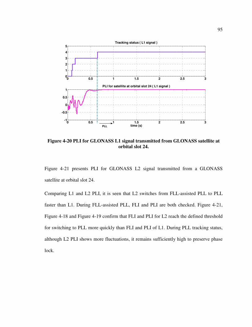
95
0 0.5 1 1.5 2 2.5 30
1
2
3
4
5Tracking status ( L1 signal )
0 0.5 1 1.5 2 2.5 3-1
-0.5
0
0.5
1PLI for satellite at orbital slot 24 ( L1 signal )
time (s)PLL
Figure 4-20 PLI for GLONASS L1 signal transmitted from GLONASS satellite at
orbital slot 24.
Figure 4-21 presents PLI for GLONASS L2 signal transmitted from a GLONASS
satellite at orbital slot 24.
Comparing L1 and L2 PLI, it is seen that L2 switches from FLL-assisted PLL to PLL
faster than L1. During FLL-assisted PLL, FLI and PLI are both checked. Figure 4-21,
Figure 4-18 and Figure 4-19 confirm that FLI and PLI for L2 reach the defined threshold
for switching to PLL more quickly than FLI and PLI of L1. During PLL tracking status,
although L2 PLI shows more fluctuations, it remains sufficiently high to preserve phase
lock.
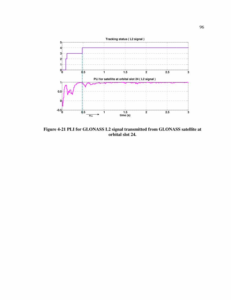
96
0 0.5 1 1.5 2 2.5 30
1
2
3
4
5Tracking status ( L2 signal )
0 0.5 1 1.5 2 2.5 3-0.5
0
0.5
1PLI for satellite at orbital slot 24 ( L2 signal )
time (s)PLL
Figure 4-21 PLI for GLONASS L2 signal transmitted from GLONASS satellite at
orbital slot 24.
97
CHAPTER FIVE: NAVIGATION SIGNAL PROCESSING
5.1 Chapter outline
At the beginning of this Chapter, the GLONASS navigation message structure is
reviewed. After that, GLONASS navigation data bit synchronization is explained. The
Chapter continues with an explanation of the method used for GLONASS navigation
string synchronization. Then, the navigation data decoding is discussed and an
experiment for verification of the whole process is illustrated. Then, the decoded
GLONASS navigation message is compared with the navigation message from a
commercial receiver and some results are presented. At the end of this Chapter, the
ionosphere-free navigation solution is discussed and some results are presented.
5.2 GLONASS navigation message structure overview
The detailed GLONASS navigation message structure is explained in section 2.6.1. A
summary of this section is presented here for convenience. According to GLONASS ICD
(2002), the GLONASS navigation message is generated as a pattern of continuously
repeating “strings” each with duration of two seconds. During the first 1.7 seconds of
each two second interval (at the beginning of each string), 85 bits of navigation data are
transmitted. During the last 0.3 seconds (at the end of each string) the time mark is
transmitted. Navigation data bits are encoded using a Hamming code of length four. In
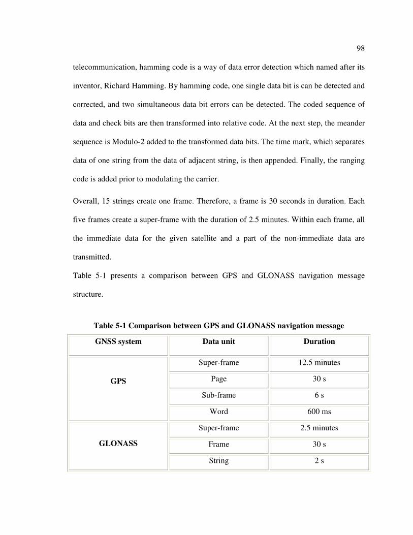
98
telecommunication, hamming code is a way of data error detection which named after its
inventor, Richard Hamming. By hamming code, one single data bit is can be detected and
corrected, and two simultaneous data bit errors can be detected. The coded sequence of
data and check bits are then transformed into relative code. At the next step, the meander
sequence is Modulo-2 added to the transformed data bits. The time mark, which separates
data of one string from the data of adjacent string, is then appended. Finally, the ranging
code is added prior to modulating the carrier.
Overall, 15 strings create one frame. Therefore, a frame is 30 seconds in duration. Each
five frames create a super-frame with the duration of 2.5 minutes. Within each frame, all
the immediate data for the given satellite and a part of the non-immediate data are
transmitted.
Table 5-1 presents a comparison between GPS and GLONASS navigation message
structure.
Table 5-1 Comparison between GPS and GLONASS navigation message
GNSS system Data unit Duration
Super-frame 12.5 minutes
Page 30 s
Sub-frame 6 s
GPS
Word 600 ms
Super-frame 2.5 minutes
Frame 30 s
GLONASS
String 2 s
99
5.3 GLONASS navigation message decoding
GLONASS navigation message is a 50 Hz message which is modulated with a 100 Hz
meander sequence by Modulo-2 addition (GLONASS ICD 2002). The GLONASS
navigation message contains information related to the satellite being tracked and also
information related to the GLONASS constellation. As such, the navigation message
must be decoded to extract this information which is necessary for computing navigation
solution. To this end, the following steps are required:
1. Bit synchronization
2. String synchronization
3. Navigation message decoding
These steps are explained more in the following sections.
5.3.1 Bit synchronization
To decode the navigation message, it is important to find the location of navigation data
bit transition. To determine the data bit transition location, a few methods are proposed
(Rambo 1989, Spilker 1977). The method which is used herein is the histogram method
(Van Deirendonck 1996). In this method, a navigation data bit is divided into shorter
bins. For GLONASS, a 10-ms data bit is divided into 10 1-ms bins. Then, the transitions
between two successive bins are detected. These transitions are recorded in counters (one
counter for each bin). The process continues until one of the three following conditions
occurs:
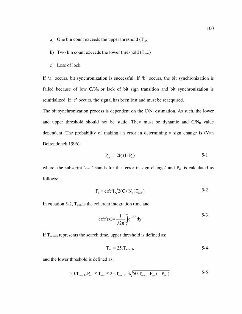
100
a) One bin count exceeds the upper threshold (Tup)
b) Two bin count exceeds the lower threshold (Tlow)
c) Loss of lock
If ‘a’ occurs, bit synchronization is successful. If ‘b’ occurs, the bit synchronization is
failed because of low C/N0 or lack of bit sign transition and bit synchronization is
reinitialized. If ‘c’ occurs, the signal has been lost and must be reacquired.
The bit synchronization process is dependent on the C/N0 estimation. As such, the lower
and upper threshold should not be static. They must be dynamic and C/N0 value
dependent. The probability of making an error in determining a sign change is (Van
Deirendonck 1996):
esc e eP = 2P (1- P ) 5-1
where, the subscript ‘esc’ stands for the ‘error in sign change’ and Pe is calculated as
follows:
e 0 cohP = erfc '[ 2(C / N )T ] 5-2
In equation 5-2, Tcoh is the coherent integration time and
2-y /2
x
1erfc (x)= e dy
2π
∞
′ ∫ 5-3
If Tsearch represents the search time, upper threshold is defined as:
Tup = 25.Tsearch 5-4
and the lower threshold is defined as:
search esc low search search esc esc50.T .P T 25.T -3 50.T .P (1-P )≤ ≤ 5-5

101
Tsearch is defined one second in the software receiver.
For GPS in Tsearch second, there are 25Tsearch data bit transitions in average and for
GLONASS in Tsearch second there are 50 Tsearch data bit transitions in average. As such, if
the counter of a bin shows a value of 25Tsearch or more for GPS and 50Tsearch or more for
GLONASS, the location of data bit transition is defined.
According to the above equations, the upper and lower thresholds are not common
amongst all satellites being tracked.
Figure 5-1 illustrates the bit synchronization for different GLONASS satellites. In this
figure, a status value of one represents the successful bit synchronization.
0.3 0.32 0.34 0.36 0.38 0.4 0.42 0.44 0.46 0.48 0.50
0.2
0.4
0.6
0.8
1
time (s)
Bit synchronization status
Ch# -2
Ch# 0
Ch# -1
Ch# 03
Ch# 02
Figure 5-1 Bit synchronization status for different GLONASS satellites
102
5.3.2 String synchronization
The next step after bit synchronization is finding the location of the string within the
received navigation message. To achieve this synchronization, some of the properties of
the GLONASS navigation message are used.
At the first step, the time mark is checked. Time mark is explained in detail in section
2.6.3. The time mark for GLONASS is roughly equivalent to the preamble for GPS. After
bit synchronization, the time mark pattern or its complement is searched. The
complement must be searched because of the uncertainty on the polarity of the locally
generated carrier signal. If the complement of the time mark is found, all the navigation
data bits must be converted into their complement values. After finding the time mark
pattern or its complement, the received data is checked after two seconds again to check
if the pattern repeats or not. If the location of the time mark is correct, it should repeat
every two seconds.
After finding the location of the time mark, the data bits are converted from 10-ms data
into 20-ms data bits by removing the effect of the 100-Hz meander sequence. In this step,
data bit pairs are converted into one bit (the reverse process of adding the meander
sequence to the data bits).
After having removed the meander code, what remain on the signal are navigation data
bits and the check bits but still it is necessary to retransform from relative code (section
2.6.3). This is done by adding each bit to the previous one by Modulo-2 addition.
Now the data bits are revealed (i.e., bits 9 to 84) but they must be verified with the
checking bits (i.e., bits 1 to 8). Figure 2-8 illustrates the location of these bits well. The

103
algorithm for data verification allows correcting an error in one bit within a string and
detecting (but not correcting) an error in two or more bits within string. To correct one bit
in a string seven checksums are generated (C1…C7) and to detect two-bit error another
checksum (CΣ) is generated. These checksums are generated as follows (GLONASS ICD
2002):
1 1 ii mod 2C =β b ⊕ ∑ 5-6
i = 9, 10, 12, 13, 15, 17, 19, 20, 22, 24, 26, 28, 30, 32, 34, 35, 37, 39, 41, 43,
45, 47, 49, 51, 53, 55, 57, 59, 61, 63, 65, 66, 68, 70, 72, 74, 76, 78, 80, 82, 84
2 2 jj mod 2C =β b ⊕
∑ 5-7
j = 9, 11, 12, 14, 15, 18, 19, 21, 22, 25, 26, 29, 30, 33, 34, 36, 37, 40, 41, 44,
45, 48, 49, 52, 53, 56, 57, 60, 61, 64, 65, 67, 68, 71, 72, 75, 76, 79, 80, 83, 84
3 3 kk mod 2C =β b ⊕ ∑ 5-8
k = 10-12, 16-19, 23-26, 31-34, 38-41, 46-49, 54-57, 62-65, 69-72, 77-80, 85
4 4 ll mod 2C =β b ⊕ ∑ 5-9
l = 13-19, 27-34, 42-49, 58-65, 73-80.
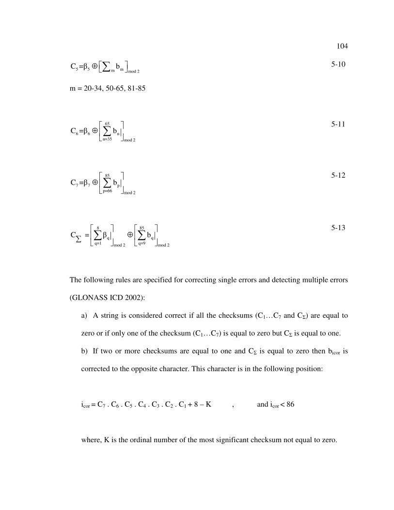
104
5 5 mm mod 2C =β b ⊕ ∑ 5-10
m = 20-34, 50-65, 81-85
65
6 6 n
n=35 mod 2
C =β b
⊕ ∑
5-11
85
7 7 p
p=66 mod 2
C =β b
⊕ ∑
5-12
8 85
q q
q=1 q=9mod 2 mod 2
C = β b
⊕ ∑ ∑ ∑
5-13
The following rules are specified for correcting single errors and detecting multiple errors
(GLONASS ICD 2002):
a) A string is considered correct if all the checksums (C1…C7 and CΣ) are equal to
zero or if only one of the checksum (C1…C7) is equal to zero but CΣ is equal to one.
b) If two or more checksums are equal to one and CΣ is equal to zero then bicor is
corrected to the opposite character. This character is in the following position:
icor = C7 . C6 . C5 . C4 . C3 . C2 . C1 + 8 – K , and icor < 86
where, K is the ordinal number of the most significant checksum not equal to zero.

105
If the icor > 85, it indicates that there is odd number of errors greater than one. Thus,
the data can not be corrected and must be ignored.
c) If at least one of the checksums (C1…C7) is equal to one and CΣ is equal to zero,
or if all the checksums (C1…C7) are equal to zero but CΣ is equal to one, there are
multiple errors and the data must be removed.
When the data verification is passed, the correct navigation data bits are revealed and
information can be extracted from the data bits. The whole process mentioned above is
the reverse process of GLONASS navigation data generation illustrated in Figure 2-9.
Block diagram presented in Figure 5-2 summarizes the method used for GLONASS
string synchronization.

106
Figure 5-2 GLONASS navigation string synchronization algorithm
Search for time mark or its
complement
Search for time
mark after 2 s
Start
End
Remove the data
Report false
data bits
Sting synchronization is achieved
Data bits verification
Transformation from relative code to
sequence of data and check bits
Yes
Remove time mark from the string
Convert the string from 10-ms to 20-ms data bits (remove meander code
effect)
No
No
Yes
Yes
No
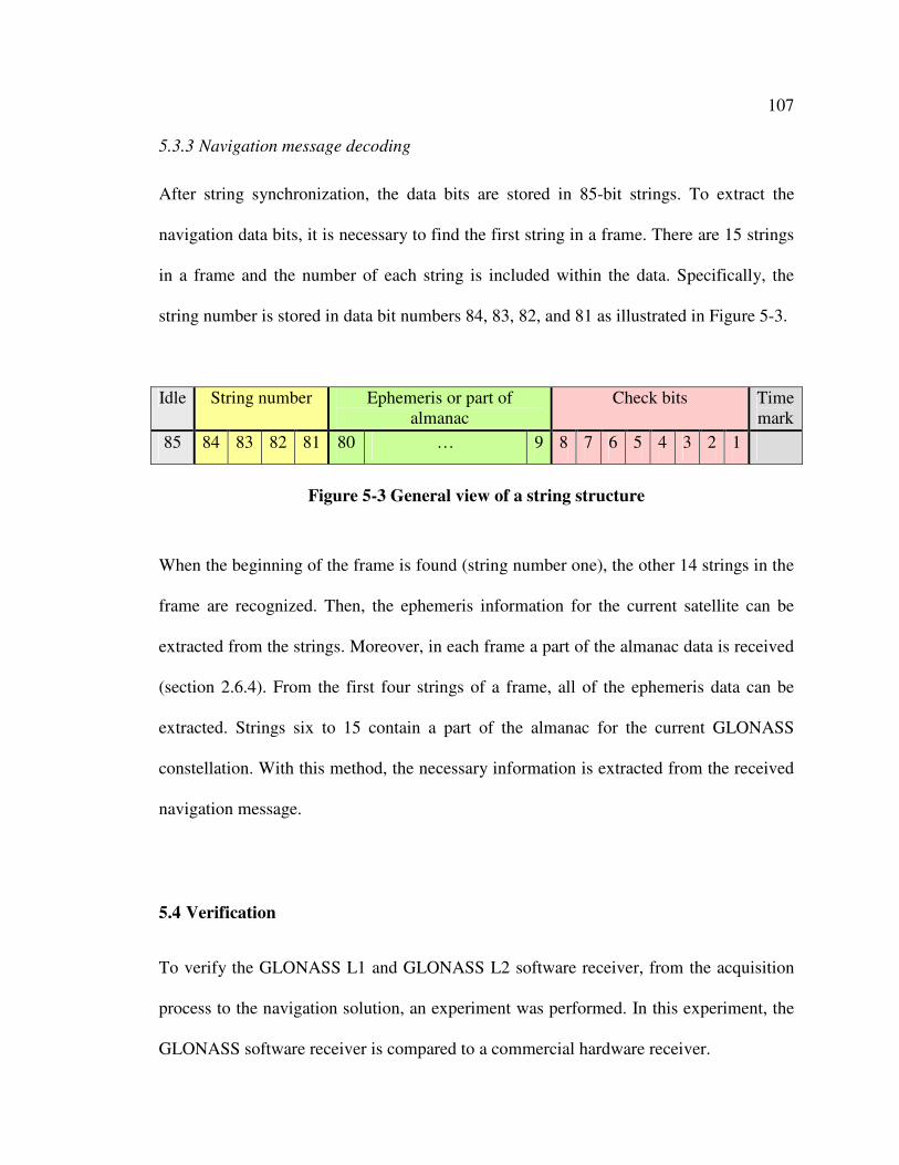
107
5.3.3 Navigation message decoding
After string synchronization, the data bits are stored in 85-bit strings. To extract the
navigation data bits, it is necessary to find the first string in a frame. There are 15 strings
in a frame and the number of each string is included within the data. Specifically, the
string number is stored in data bit numbers 84, 83, 82, and 81 as illustrated in Figure 5-3.
Idle String number Ephemeris or part of almanac
Check bits Time mark
85 84 83 82 81 80 … 9 8 7 6 5 4 3 2 1
Figure 5-3 General view of a string structure
When the beginning of the frame is found (string number one), the other 14 strings in the
frame are recognized. Then, the ephemeris information for the current satellite can be
extracted from the strings. Moreover, in each frame a part of the almanac data is received
(section 2.6.4). From the first four strings of a frame, all of the ephemeris data can be
extracted. Strings six to 15 contain a part of the almanac for the current GLONASS
constellation. With this method, the necessary information is extracted from the received
navigation message.
5.4 Verification
To verify the GLONASS L1 and GLONASS L2 software receiver, from the acquisition
process to the navigation solution, an experiment was performed. In this experiment, the
GLONASS software receiver is compared to a commercial hardware receiver.
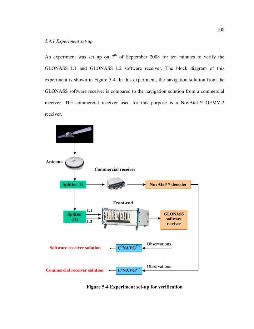
108
5.4.1 Experiment set-up
An experiment was set up on 7th of September 2008 for ten minutes to verify the
GLONASS L1 and GLONASS L2 software receiver. The block diagram of this
experiment is shown in Figure 5-4. In this experiment, the navigation solution from the
GLONASS software receiver is compared to the navigation solution from a commercial
receiver. The commercial receiver used for this purpose is a NovAtel™ OEMV-2
receiver.
Figure 5-4 Experiment set-up for verification
Splitter (I)
L1
Commercial receiver
Antenna
Splitter
(II) L2
GLONASS
software
receiver
Observations
Software receiver solution
Front-end
C3NAVG
2™ Commercial receiver solution
Observations C
3NAVG
2™
NovAtel™ deocder

109
The received signal from the antenna is sent to the splitter (I). One of the signals from the
splitter is sent to the NovAtel™ receiver which was configured to log the raw
measurement data. The other signal from the splitter is sent to yet another splitter (splitter
II). The outputs of the second splitter are defined as L1 and L2 and sent to different RF
input on the front-end.
In this experiment, raw measurement data is collected from the NovAtel™ receiver and
sent to some NovAtel™ decoder software which is capable of generating GLONASS
ephemeris and observation files in post-mission. The ephemeris file contains ephemeris
information for all GLONASS satellites. The observation file contains pseudorange,
carrier phase and Doppler frequency for L1 and L2 signals. These two files are fed into a
software package called C3NAVG2™. This software was developed in the Position,
Location And Navigation (PLAN) group at the department of Geomatics Engineering.
C3NAVG2™
is a C program that processes GPS and/or GLONASS pseudorange data in
both static and kinematic modes. One of the outputs of this software is the position of the
antenna at each epoch. In this way, the position of the antenna determined by the
commercial receiver is calculated.
In parallel with the NovAtel™ data collection, the GLONASS L1 and L2 samples were
logged from the front-end. These samples were then processed by the GLONASS
software receiver (GSNRx™) developed as part of this thesis.
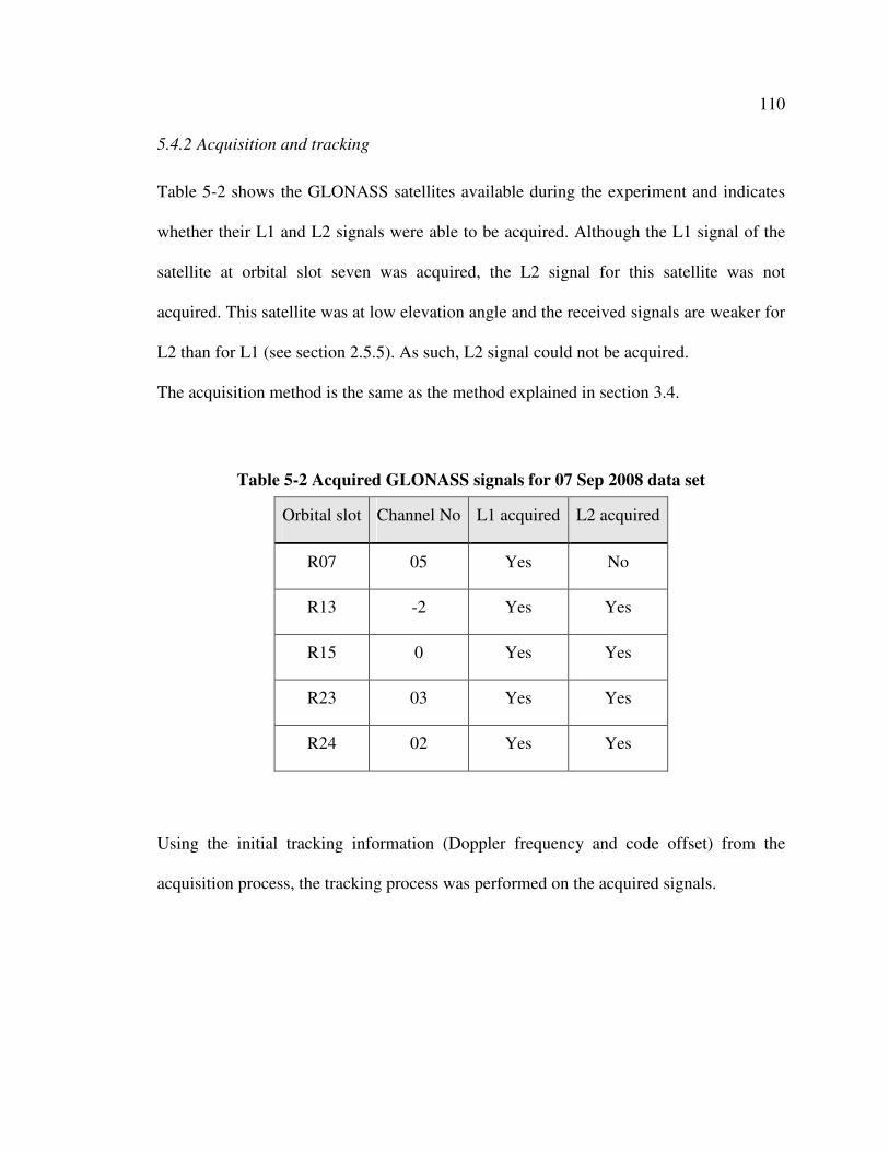
110
5.4.2 Acquisition and tracking
Table 5-2 shows the GLONASS satellites available during the experiment and indicates
whether their L1 and L2 signals were able to be acquired. Although the L1 signal of the
satellite at orbital slot seven was acquired, the L2 signal for this satellite was not
acquired. This satellite was at low elevation angle and the received signals are weaker for
L2 than for L1 (see section 2.5.5). As such, L2 signal could not be acquired.
The acquisition method is the same as the method explained in section 3.4.
Table 5-2 Acquired GLONASS signals for 07 Sep 2008 data set
Orbital slot Channel No L1 acquired L2 acquired
R07 05 Yes No
R13 -2 Yes Yes
R15 0 Yes Yes
R23 03 Yes Yes
R24 02 Yes Yes
Using the initial tracking information (Doppler frequency and code offset) from the
acquisition process, the tracking process was performed on the acquired signals.
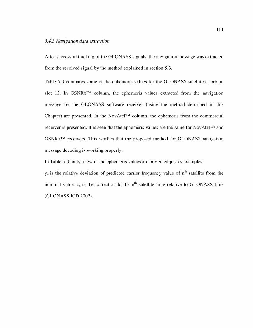
111
5.4.3 Navigation data extraction
After successful tracking of the GLONASS signals, the navigation message was extracted
from the received signal by the method explained in section 5.3.
Table 5-3 compares some of the ephemeris values for the GLONASS satellite at orbital
slot 13. In GSNRx™ column, the ephemeris values extracted from the navigation
message by the GLONASS software receiver (using the method described in this
Chapter) are presented. In the NovAtel™ column, the ephemeris from the commercial
receiver is presented. It is seen that the ephemeris values are the same for NovAtel™ and
GSNRx™ receivers. This verifies that the proposed method for GLONASS navigation
message decoding is working properly.
In Table 5-3, only a few of the ephemeris values are presented just as examples.
γn is the relative deviation of predicted carrier frequency value of nth satellite from the
nominal value. τn is the correction to the nth satellite time relative to GLONASS time
(GLONASS ICD 2002).
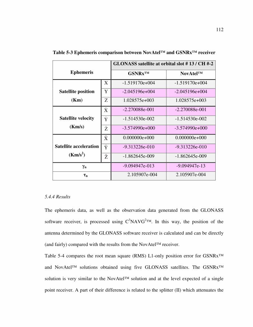
112
Table 5-3 Ephemeris comparison between NovAtel™ and GSNRx™ receiver
GLONASS satellite at orbital slot # 13 / CH #-2
Ephemeris GSNRx™ NovAtel™
X -1.519170e+004 -1.519170e+004
Y -2.045196e+004 -2.045196e+004
Satellite position
(Km) Z 1.028575e+003 1.028575e+003
Xɺ -2.270088e-001 -2.270088e-001
Yɺ -1.514530e-002 -1.514530e-002
Satellite velocity
(Km/s) Zɺ -3.574990e+000 -3.574990e+000
Xɺɺ 0.000000e+000 0.000000e+000
Yɺɺ -9.313226e-010 -9.313226e-010
Satellite acceleration
(Km/s2) Zɺɺ -1.862645e-009 -1.862645e-009
γn -9.094947e-013 -9.094947e-13
τn 2.105907e-004 2.105907e-004
5.4.4 Results
The ephemeris data, as well as the observation data generated from the GLONASS
software receiver, is processed using C3NAVG2™. In this way, the position of the
antenna determined by the GLONASS software receiver is calculated and can be directly
(and fairly) compared with the results from the NovAtel™ receiver.
Table 5-4 compares the root mean square (RMS) L1-only position error for GSNRx™
and NovAtel™ solutions obtained using five GLONASS satellites. The GSNRx™
solution is very similar to the NovAtel™ solution and at the level expected of a single
point receiver. A part of their difference is related to the splitter (II) which attenuates the
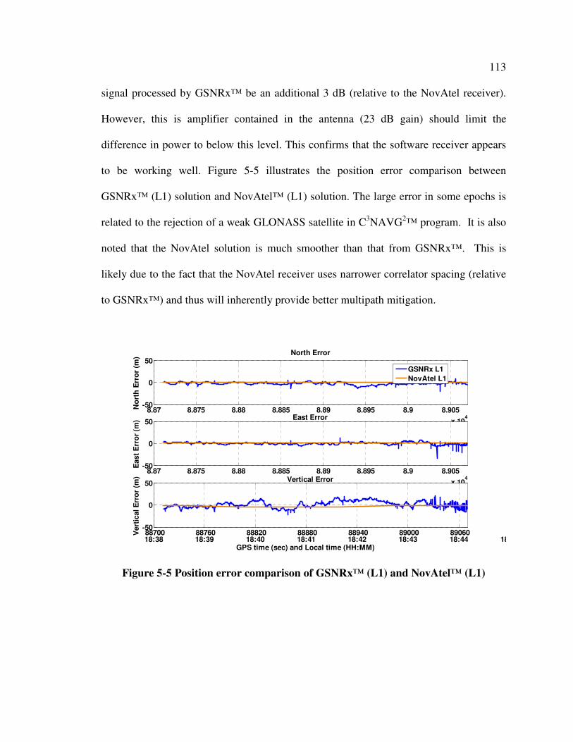
113
signal processed by GSNRx™ be an additional 3 dB (relative to the NovAtel receiver).
However, this is amplifier contained in the antenna (23 dB gain) should limit the
difference in power to below this level. This confirms that the software receiver appears
to be working well. Figure 5-5 illustrates the position error comparison between
GSNRx™ (L1) solution and NovAtel™ (L1) solution. The large error in some epochs is
related to the rejection of a weak GLONASS satellite in C3NAVG2™ program. It is also
noted that the NovAtel solution is much smoother than that from GSNRx™. This is
likely due to the fact that the NovAtel receiver uses narrower correlator spacing (relative
to GSNRx™) and thus will inherently provide better multipath mitigation.
8.87 8.875 8.88 8.885 8.89 8.895 8.9 8.905
x 104
-50
0
50
No
rth
Err
or
(m)
North Error
GSNRx L1
NovAtel L1
8.87 8.875 8.88 8.885 8.89 8.895 8.9 8.905
x 104
-50
0
50
East
Err
or
(m) East Error
88700 88760 88820 88880 88940 89000 89060-50
0
50
Vert
ical E
rro
r (m
) Vertical Error
18:38 18:39 18:40 18:41 18:42 18:43 18:44 18:45GPS time (sec) and Local time (HH:MM)
Figure 5-5 Position error comparison of GSNRx™ (L1) and NovAtel™ (L1)

114
Table 5-4 Root Means Square (RMS) position errors for GSNRx™ and NovAtel™
Solution North East Vertical
GSNRx™ (L1) 2.1 m 2.8 m 7.5 m
NovAtel™ (L1) 0.5 m 1.7 m 2.8 m
Moreover, the position solution results for L1 and L2 from GSNRx™ are shown in
Figure 5-6. The same satellites are tracked in both cases in order to remove any effect due
to different satellite geometry.
8.87 8.88 8.89 8.9 8.91 8.92 8.93
x 104
-20
0
20
No
rth
Err
or
(m) North Error
L1
L2
8.87 8.88 8.89 8.9 8.91 8.92 8.93
x 104
-20
0
20East Error
East
Err
or
(m)
88700 88760 88820 88880 88940 89000 89060 89120 89180 89240 89300-50
0
50
18:38 18:39 18:40 18:41 18:42 18:43 18:44 18:45 18:46 18:47 18:48GPS time (sec) and Local time (HH:MM)
Vertical Error
Vert
ical E
rro
r (m
)
Figure 5-6 Position error comparison of L1 and L2 computed using GSNRx™
Table 5-5 compares the root mean square (RMS) value of the position error for L1-only
and L2-only solutions. This table shows that the RMS position errors for L1-only and L2-
only solutions are approximately the same which is expected under calm ionospheric
condition which was present during the test. For these solutions, only the four satellites
for which the L2 data is available are used (even for L1 solution) in order to avoid effects
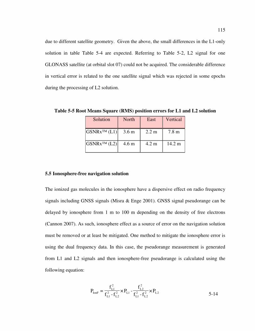
115
due to different satellite geometry. Given the above, the small differences in the L1-only
solution in table Table 5-4 are expected. Referring to Table 5-2, L2 signal for one
GLONASS satellite (at orbital slot 07) could not be acquired. The considerable difference
in vertical error is related to the one satellite signal which was rejected in some epochs
during the processing of L2 solution.
Table 5-5 Root Means Square (RMS) position errors for L1 and L2 solution
Solution North East Vertical
GSNRx™ (L1) 3.6 m 2.2 m 7.8 m
GSNRx™ (L2) 4.6 m 4.2 m 14.2 m
5.5 Ionosphere-free navigation solution
The ionized gas molecules in the ionosphere have a dispersive effect on radio frequency
signals including GNSS signals (Misra & Enge 2001). GNSS signal pseudorange can be
delayed by ionosphere from 1 m to 100 m depending on the density of free electrons
(Cannon 2007). As such, ionosphere effect as a source of error on the navigation solution
must be removed or at least be mitigated. One method to mitigate the ionosphere error is
using the dual frequency data. In this case, the pseudorange measurement is generated
from L1 and L2 signals and then ionosphere-free pseudorange is calculated using the
following equation:
2 2
L1 L2
2 2 2 2IonF L1 L2
L1 L2 L1 L2
f fP = × P - ×P
f - f f - f
5-14
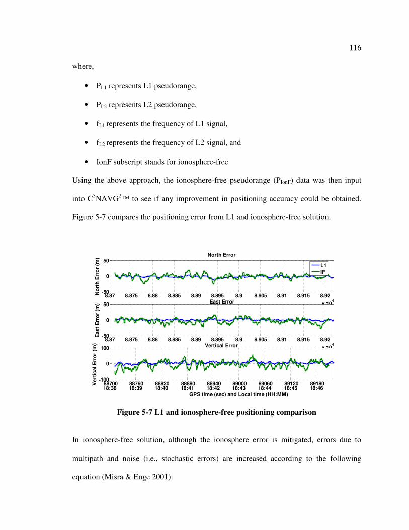
116
where,
• PL1 represents L1 pseudorange,
• PL2 represents L2 pseudorange,
• fL1 represents the frequency of L1 signal,
• fL2 represents the frequency of L2 signal, and
• IonF subscript stands for ionosphere-free
Using the above approach, the ionosphere-free pseudorange (PIonF) data was then input
into C3NAVG2™ to see if any improvement in positioning accuracy could be obtained.
Figure 5-7 compares the positioning error from L1 and ionosphere-free solution.
8.87 8.875 8.88 8.885 8.89 8.895 8.9 8.905 8.91 8.915 8.92
x 104
-50
0
50
No
rth
Err
or
(m)
North Error
L1
IF
8.87 8.875 8.88 8.885 8.89 8.895 8.9 8.905 8.91 8.915 8.92
x 104
-50
0
50East Error
East
Err
or
(m)
88700 88760 88820 88880 88940 89000 89060 89120 89180-100
0
100
18:38 18:39 18:40 18:41 18:42 18:43 18:44 18:45 18:46
GPS time (sec) and Local time (HH:MM)
Vertical Error
Vert
ical E
rro
r (m
)
Figure 5-7 L1 and ionosphere-free positioning comparison
In ionosphere-free solution, although the ionosphere error is mitigated, errors due to
multipath and noise (i.e., stochastic errors) are increased according to the following
equation (Misra & Enge 2001):
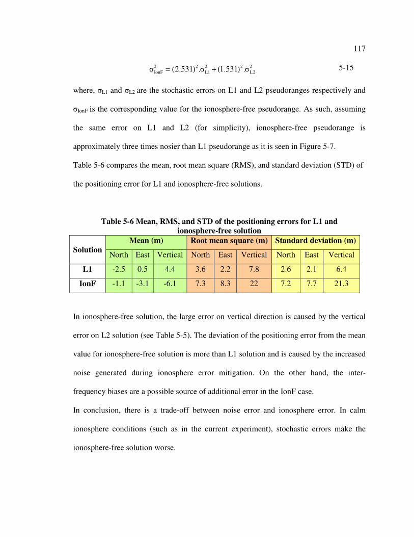
117
2 2 2 2 2
IonF L1 L2σ = (2.531) .σ + (1.531) .σ 5-15
where, σL1 and σL2 are the stochastic errors on L1 and L2 pseudoranges respectively and
σIonF is the corresponding value for the ionosphere-free pseudorange. As such, assuming
the same error on L1 and L2 (for simplicity), ionosphere-free pseudorange is
approximately three times nosier than L1 pseudorange as it is seen in Figure 5-7.
Table 5-6 compares the mean, root mean square (RMS), and standard deviation (STD) of
the positioning error for L1 and ionosphere-free solutions.
Table 5-6 Mean, RMS, and STD of the positioning errors for L1 and
ionosphere-free solution
Mean (m) Root mean square (m) Standard deviation (m)
Solution North East Vertical North East Vertical North East Vertical
L1 -2.5 0.5 4.4 3.6 2.2 7.8 2.6 2.1 6.4
IonF -1.1 -3.1 -6.1 7.3 8.3 22 7.2 7.7 21.3
In ionosphere-free solution, the large error on vertical direction is caused by the vertical
error on L2 solution (see Table 5-5). The deviation of the positioning error from the mean
value for ionosphere-free solution is more than L1 solution and is caused by the increased
noise generated during ionosphere error mitigation. On the other hand, the inter-
frequency biases are a possible source of additional error in the IonF case.
In conclusion, there is a trade-off between noise error and ionosphere error. In calm
ionosphere conditions (such as in the current experiment), stochastic errors make the
ionosphere-free solution worse.

118
CHAPTER SIX: GLONASS+GPS SOFTWARE RECEIVER
6.1 Chapter outline
The objective of this Chapter is to present a software receiver capable of simultaneously
tracking GPS L1, GLONASS L1 and GLONASS L2 signals (herein termed a “combined
software receiver”) and providing navigation solution. To begin, there is a brief
discussion on the differences and similarities of GPS and GLONASS systems. The
Chapter continues with the explanation of the required modifications in GSNRx™. The
Chapter concludes some results from the combined software receiver compared with the
results from single (GPS alone, GLONASS L1 alone and GLONASS L2 alone) software
receivers. At the end of the Chapter, positioning for the combined software receiver is
presented and compared to the single systems.
For simplicity, the term “GPS” is used instead of “GPS L1” throughout the Chapter.
6.2 Differences and similarities of GPS and GLONASS
As discussed in Chapter one, the GLONASS system can be used to augment GPS system.
With the recent revitalization of GLONASS (constellation status shown in Figure 2-1),
the combination of GPS and GLONASS helps achieving more reliable and accurate
navigation solutions. Combination of GLONASS L1 and GLONASS L2 helps reducing
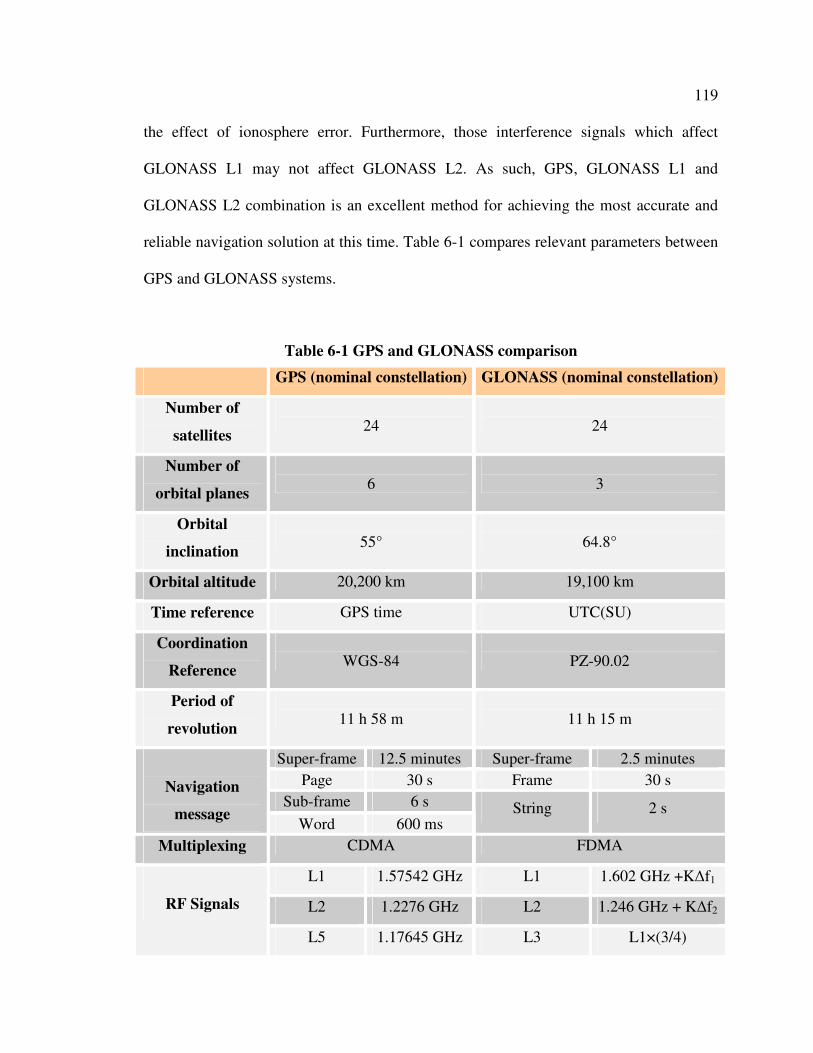
119
the effect of ionosphere error. Furthermore, those interference signals which affect
GLONASS L1 may not affect GLONASS L2. As such, GPS, GLONASS L1 and
GLONASS L2 combination is an excellent method for achieving the most accurate and
reliable navigation solution at this time. Table 6-1 compares relevant parameters between
GPS and GLONASS systems.
Table 6-1 GPS and GLONASS comparison
GPS (nominal constellation) GLONASS (nominal constellation)
Number of
satellites
24
24
Number of
orbital planes
6
3
Orbital
inclination
55°
64.8°
Orbital altitude 20,200 km 19,100 km
Time reference GPS time UTC(SU)
Coordination
Reference
WGS-84
PZ-90.02
Period of
revolution
11 h 58 m
11 h 15 m
Super-frame 12.5 minutes Super-frame 2.5 minutes
Page 30 s Frame 30 s
Sub-frame 6 s
Navigation
message Word 600 ms
String 2 s
Multiplexing CDMA FDMA
L1 1.57542 GHz L1 1.602 GHz +K∆f1
L2 1.2276 GHz L2 1.246 GHz + K∆f2
RF Signals
L5 1.17645 GHz L3 L1×(3/4)
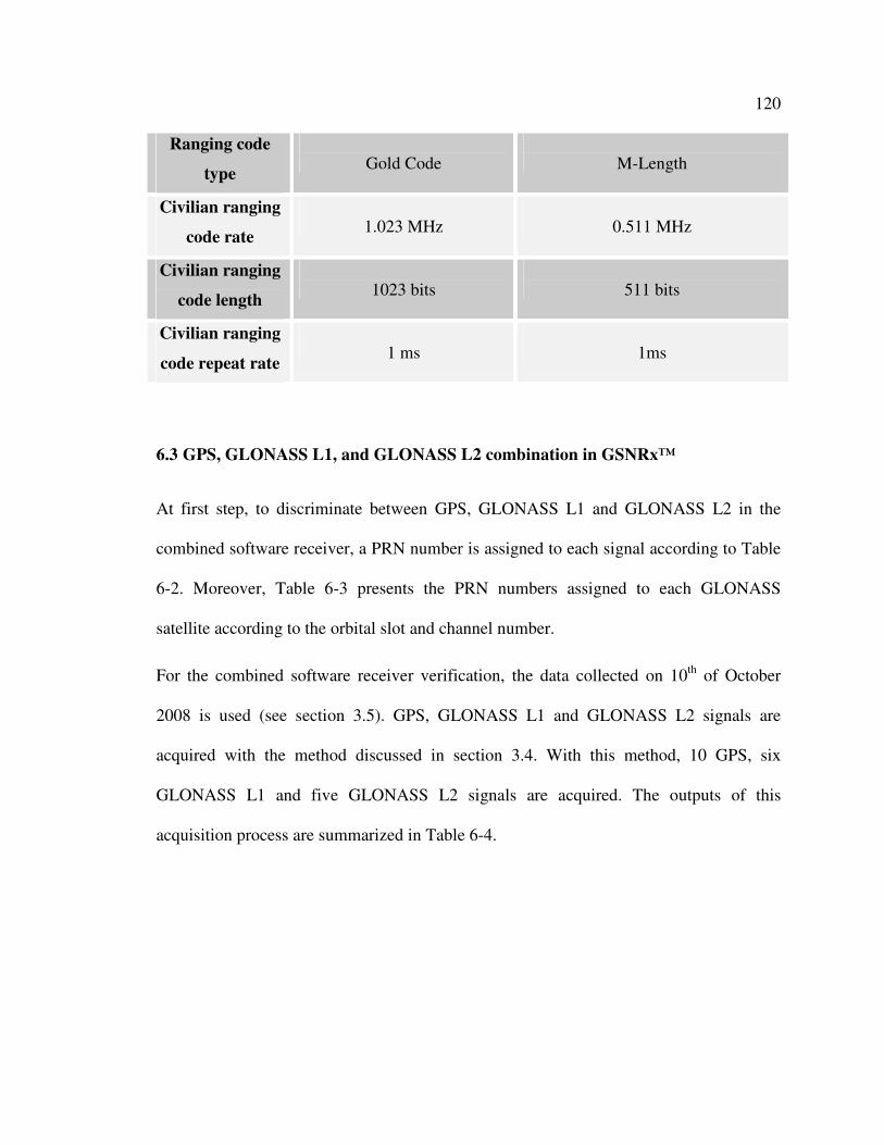
120
Ranging code
type
Gold Code
M-Length
Civilian ranging
code rate
1.023 MHz
0.511 MHz
Civilian ranging
code length
1023 bits
511 bits
Civilian ranging
code repeat rate
1 ms
1ms
6.3 GPS, GLONASS L1, and GLONASS L2 combination in GSNRx™
At first step, to discriminate between GPS, GLONASS L1 and GLONASS L2 in the
combined software receiver, a PRN number is assigned to each signal according to Table
6-2. Moreover, Table 6-3 presents the PRN numbers assigned to each GLONASS
satellite according to the orbital slot and channel number.
For the combined software receiver verification, the data collected on 10th of October
2008 is used (see section 3.5). GPS, GLONASS L1 and GLONASS L2 signals are
acquired with the method discussed in section 3.4. With this method, 10 GPS, six
GLONASS L1 and five GLONASS L2 signals are acquired. The outputs of this
acquisition process are summarized in Table 6-4.
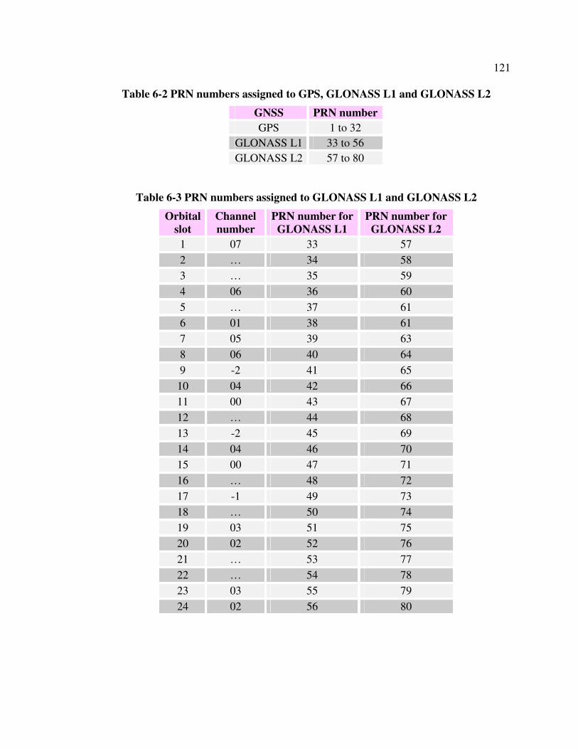
121
Table 6-2 PRN numbers assigned to GPS, GLONASS L1 and GLONASS L2
GNSS PRN number
GPS 1 to 32
GLONASS L1 33 to 56
GLONASS L2 57 to 80
Table 6-3 PRN numbers assigned to GLONASS L1 and GLONASS L2
Orbital
slot
Channel
number
PRN number for
GLONASS L1
PRN number for
GLONASS L2
1 07 33 57
2 … 34 58
3 … 35 59
4 06 36 60
5 … 37 61
6 01 38 61
7 05 39 63
8 06 40 64
9 -2 41 65
10 04 42 66
11 00 43 67
12 … 44 68
13 -2 45 69
14 04 46 70
15 00 47 71
16 … 48 72
17 -1 49 73
18 … 50 74
19 03 51 75
20 02 52 76
21 … 53 77
22 … 54 78
23 03 55 79
24 02 56 80
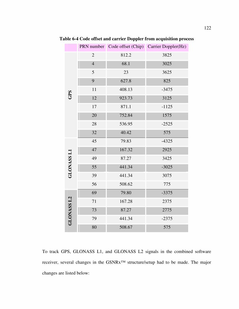
122
Table 6-4 Code offset and carrier Doppler from acquisition process
PRN number Code offset (Chip) Carrier Doppler(Hz)
2 812.2 3825
4 68.1 3025
5 23 3625
9 627.8 825
11 408.13 -3475
12 923.73 3125
17 871.1 -1125
20 752.84 1575
28 536.95 -2525
GP
S
32 40.42 575
45 79.83 -4325
47 167.32 2925
49 87.27 3425
55 441.34 -3025
39 441.34 3075 GL
ON
AS
S L
1
56 508.62 775
69 79.80 -3375
71 167.28 2375
73 87.27 2775
79 441.34 -2375
GL
ON
AS
S L
2
80 508.67 575
To track GPS, GLONASS L1, and GLONASS L2 signals in the combined software
receiver, several changes in the GSNRx™ structure/setup had to be made. The major
changes are listed below:
123
1. Input samples: the software must be able to read real samples from three input
files, namely one for GPS, one for GLONASS L1 and one for GLONASS L2.
2. Intermediate frequency: GPS intermediate frequency is different from GLONASS
intermediate frequency. As such, according to the PRN number, the correct
intermediate frequency must be generated within the software. For GPS, the
intermediate frequency is 4.42 MHz and for GLONASS is 4 MHz.
3. Maximum coherent integration time: This value can be extended to 20 ms for
GPS and to 10 ms for GLONASS because the received GLONASS navigation
data bit is 10 ms.
4. PRN number: presented in Table 6-2, the PRN numbers should be different for
GPS, GLONASS L1 and GLONASS L2.
5. Ranging code: the software must be capable of generating both the GPS and
GLONASS standard ranging codes, as appropriate, for the satellite signal being
tracked.
6. Bit synchronization: referring to section 5.3.1, one GLONASS navigation data bit
is divided into 10 1-ms bins for bit synchronization; however a GPS navigation
data bit is divided into 20 1-ms bins. This difference must be considered in the
software for bit synchronization.
Initial tracking information (initial carrier Doppler and initial code offset) are fed into the
software with an option file as explained in section 4.8.2. Other parameters not listed
above remain the same for both GPS and GLONASS. For example, the sample rate is

124
12.5 MSps for GPS, GLONASS L1 and GLONASS L2. Also, the selected tracking loop
bandwidths are the same.
The main difference between GLONASS L1 and GLONASS L2 is the final intermediate
frequency. It means that 4 MHz intermediate frequency is, in fact, the centre frequency.
The final intermediate frequency is generated according to the channel number of each
acquired GLONASS signal as follows:
Final intermediate frequency for GLONASS = 4 MHz + K×∆f1or2
where K is the channel number and ∆f is different for GLONASS L1 and GLONASS L2
signals (section 2.5.1).
Some of the tracking results are presented in the next section.
6.4 Tracking results
The combined software receiver is capable of tracking GPS, GLONASS L1 and
GLONASS L2 satellites using the initial tracking information presented in Table 6-4.
In this section C/N0 estimation, FLI and PLI results are presented for a single software
receiver and the combined software receiver for GPS, GLONASS L1 and GLONASS L2
signals.
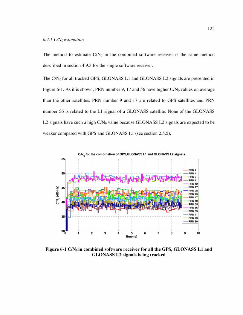
125
6.4.1 C/N0 estimation
The method to estimate C/N0 in the combined software receiver is the same method
described in section 4.9.3 for the single software receiver.
The C/N0 for all tracked GPS, GLONASS L1 and GLONASS L2 signals are presented in
Figure 6-1. As it is shown, PRN number 9, 17 and 56 have higher C/N0 values on average
than the other satellites. PRN number 9 and 17 are related to GPS satellites and PRN
number 56 is related to the L1 signal of a GLONASS satellite. None of the GLONASS
L2 signals have such a high C/N0 value because GLONASS L2 signals are expected to be
weaker compared with GPS and GLONASS L1 (see section 2.5.5).
0 1 2 3 4 5 6 7 8 9 1030
35
40
45
50
55
time (s)
C/N
0 (
dB
-Hz)
C/N0 for the combination of GPS,GLONASS L1 and GLONASS L2 signals
PRN 2
PRN 4
PRN 9
PRN 11
PRN 12
PRN 17
PRN 28
PRN 45
PRN 47
PRN 49
PRN 55
PRN 56
PRN 69
PRN 71
PRN 73
PRN 80
Figure 6-1 C/N0 in combined software receiver for all the GPS, GLONASS L1 and
GLONASS L2 signals being tracked
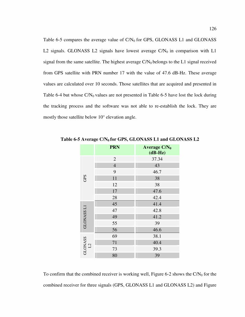
126
Table 6-5 compares the average value of C/N0 for GPS, GLONASS L1 and GLONASS
L2 signals. GLONASS L2 signals have lowest average C/N0 in comparison with L1
signal from the same satellite. The highest average C/N0 belongs to the L1 signal received
from GPS satellite with PRN number 17 with the value of 47.6 dB-Hz. These average
values are calculated over 10 seconds. Those satellites that are acquired and presented in
Table 6-4 but whose C/N0 values are not presented in Table 6-5 have lost the lock during
the tracking process and the software was not able to re-establish the lock. They are
mostly those satellite below 10° elevation angle.
Table 6-5 Average C/N0 for GPS, GLONASS L1 and GLONASS L2
PRN Average C/N0
(dB-Hz)
2 37.34
4 43
9 46.7
11 38
12 38
17 47.6
GP
S
28 42.4
45 41.4
47 42.8
49 41.2
55 39
GL
ON
AS
S L
1
56 46.6
69 38.1
71 40.4
73 39.3
GL
ON
AS
S
L2
80 39
To confirm that the combined receiver is working well, Figure 6-2 shows the C/N0 for the
combined receiver for three signals (GPS, GLONASS L1 and GLONASS L2) and Figure
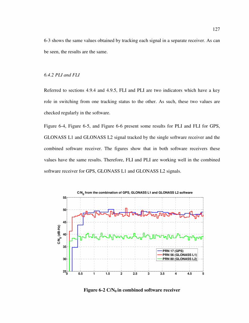
127
6-3 shows the same values obtained by tracking each signal in a separate receiver. As can
be seen, the results are the same.
6.4.2 PLI and FLI
Referred to sections 4.9.4 and 4.9.5, FLI and PLI are two indicators which have a key
role in switching from one tracking status to the other. As such, these two values are
checked regularly in the software.
Figure 6-4, Figure 6-5, and Figure 6-6 present some results for PLI and FLI for GPS,
GLONASS L1 and GLONASS L2 signal tracked by the single software receiver and the
combined software receiver. The figures show that in both software receivers these
values have the same results. Therefore, FLI and PLI are working well in the combined
software receiver for GPS, GLONASS L1 and GLONASS L2 signals.
0 0.5 1 1.5 2 2.5 3 3.5 4 4.5 525
30
35
40
45
50
55
C/N
0 (
dB
-Hz)
C/N0 from the combination of GPS, GLONASS L1 and GLONASS L2 software
PRN 17 (GPS)
PRN 56 (GLONASS L1)
PRN 80 (GLONASS L2)
Figure 6-2 C/N0 in combined software receiver
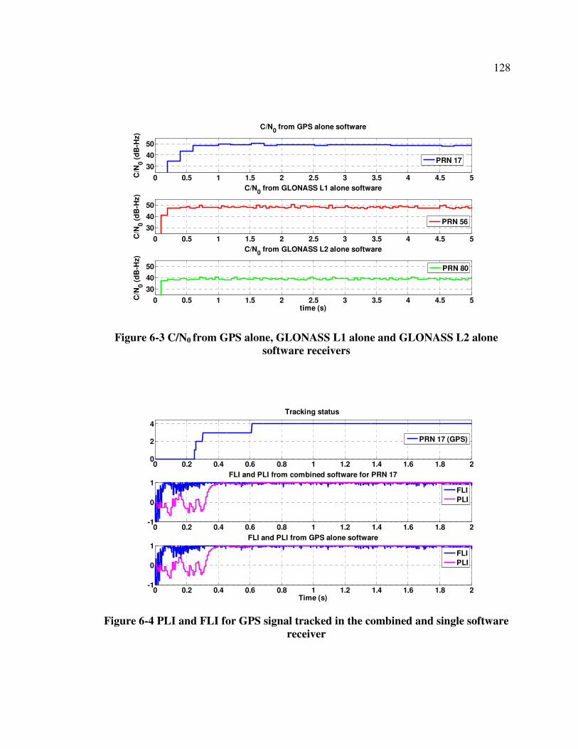
128
0 0.5 1 1.5 2 2.5 3 3.5 4 4.5 5
30
40
50
C/N0 from GPS alone software
C/N
0 (
dB
-Hz)
PRN 17
0 0.5 1 1.5 2 2.5 3 3.5 4 4.5 5
30
40
50
C/N
0 (
dB
-Hz)
C/N0 from GLONASS L1 alone software
PRN 56
0 0.5 1 1.5 2 2.5 3 3.5 4 4.5 5
30
40
50
time (s)
C/N
0 (
dB
-Hz)
C/N0 from GLONASS L2 alone software
PRN 80
Figure 6-3 C/N0 from GPS alone, GLONASS L1 alone and GLONASS L2 alone
software receivers
0 0.2 0.4 0.6 0.8 1 1.2 1.4 1.6 1.8 20
2
4
Tracking status
PRN 17 (GPS)
0 0.2 0.4 0.6 0.8 1 1.2 1.4 1.6 1.8 2-1
0
1FLI and PLI from combined software for PRN 17
FLI
PLI
0 0.2 0.4 0.6 0.8 1 1.2 1.4 1.6 1.8 2-1
0
1FLI and PLI from GPS alone software
Time (s)
FLI
PLI
Figure 6-4 PLI and FLI for GPS signal tracked in the combined and single software
receiver
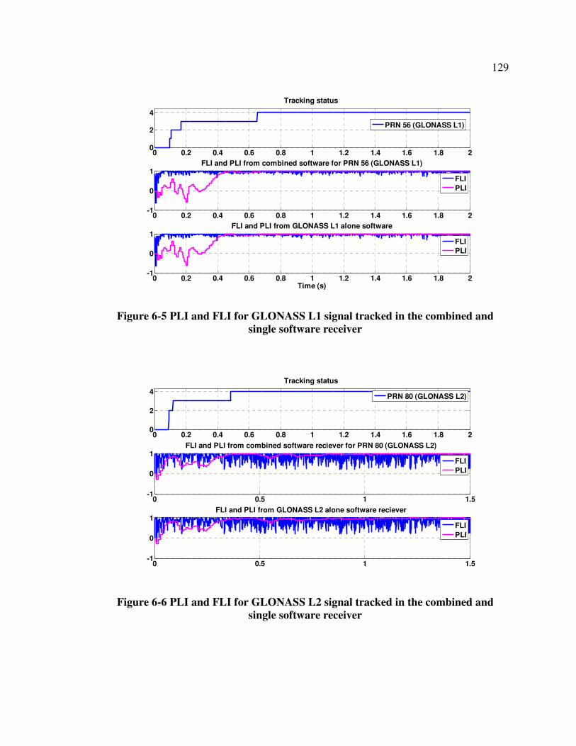
129
0 0.2 0.4 0.6 0.8 1 1.2 1.4 1.6 1.8 20
2
4
Tracking status
PRN 56 (GLONASS L1)
0 0.2 0.4 0.6 0.8 1 1.2 1.4 1.6 1.8 2-1
0
1FLI and PLI from combined software for PRN 56 (GLONASS L1)
FLI
PLI
0 0.2 0.4 0.6 0.8 1 1.2 1.4 1.6 1.8 2-1
0
1FLI and PLI from GLONASS L1 alone software
Time (s)
FLI
PLI
Figure 6-5 PLI and FLI for GLONASS L1 signal tracked in the combined and
single software receiver
0 0.2 0.4 0.6 0.8 1 1.2 1.4 1.6 1.8 20
2
4
Tracking status
PRN 80 (GLONASS L2)
0 0.5 1 1.5-1
0
1FLI and PLI from combined software reciever for PRN 80 (GLONASS L2)
FLI
PLI
0 0.5 1 1.5-1
0
1FLI and PLI from GLONASS L2 alone software reciever
FLI
PLI
Figure 6-6 PLI and FLI for GLONASS L2 signal tracked in the combined and
single software receiver
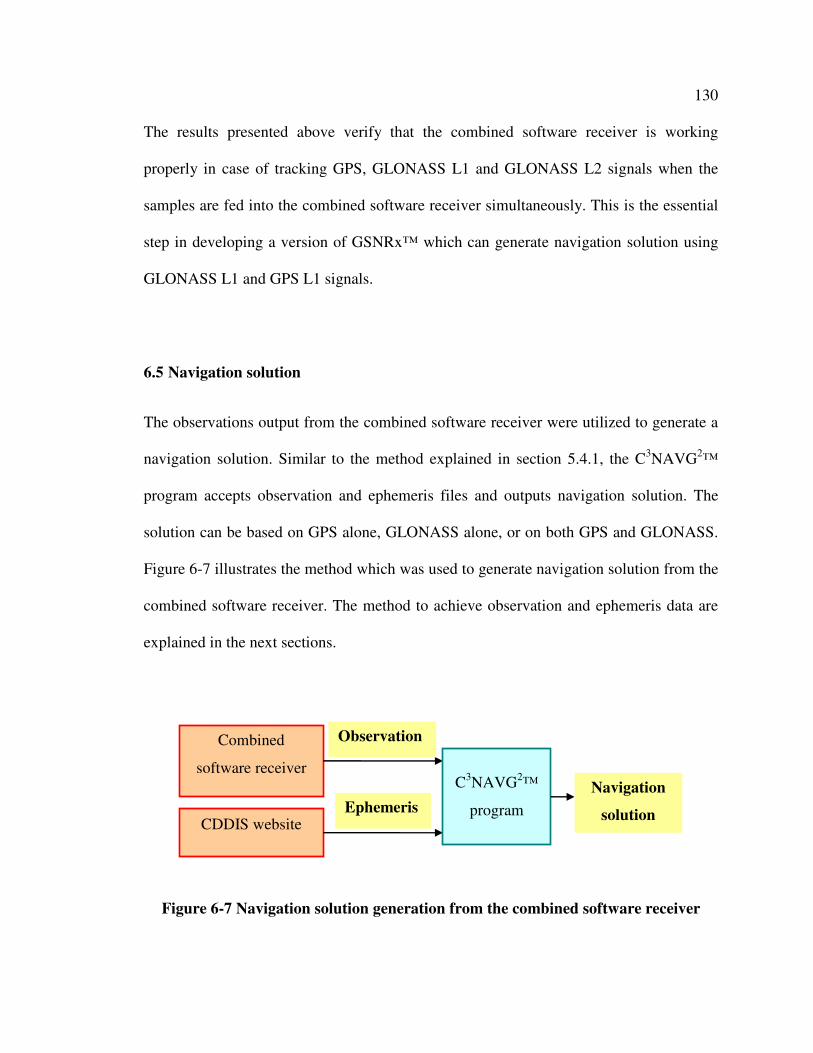
130
The results presented above verify that the combined software receiver is working
properly in case of tracking GPS, GLONASS L1 and GLONASS L2 signals when the
samples are fed into the combined software receiver simultaneously. This is the essential
step in developing a version of GSNRx™ which can generate navigation solution using
GLONASS L1 and GPS L1 signals.
6.5 Navigation solution
The observations output from the combined software receiver were utilized to generate a
navigation solution. Similar to the method explained in section 5.4.1, the C3NAVG2™
program accepts observation and ephemeris files and outputs navigation solution. The
solution can be based on GPS alone, GLONASS alone, or on both GPS and GLONASS.
Figure 6-7 illustrates the method which was used to generate navigation solution from the
combined software receiver. The method to achieve observation and ephemeris data are
explained in the next sections.
Figure 6-7 Navigation solution generation from the combined software receiver
Combined
software receiver
CDDIS website
C3NAVG2™
program
Observation
Ephemeris
Navigation
solution
131
6.5.1 Observations
The combined software receiver can generate the observation for both GPS and
GLONASS L1 and if necessary GLONASS L2. For the purpose of this section, only the
observation from GPS and GLONASS L1 are generated. In case of simplicity, the term
“GLONASS” is used instead of “GLONASS L1” from now on. The main concern in
generation of the observations for the combined GPS and GLONASS is the time
difference between GPS and GLONASS system (see section 2.7).
6.5.2 Ephemeris
Although GLONASS ephemeris can be extracted from the navigation message using the
algorithm explained in section 5.3.3, for the sake of simplicity, the ephemeris data for
GLONASS L1 and GPS L1 signals on 10th of October 2008 was acquired separately from
the NASA’s Archive of Geodesy Data (CDDIS 2008) website. After being unzipped and
conversion from RINEX format, GPS and GLONASS ephemeris were combined in a
single file and fed into the C3NAVG2™.
6.5.3 Results
Positioning results from the combined software receiver is compared to the positioning
results from a GPS alone and GLONASS alone software receiver in Figure 6-8.

132
5.0846 5.0848 5.085 5.0852 5.0854 5.0856 5.0858 5.086 5.0862 5.0864
x 105
-20
0
20North Error
No
rth
Err
or
(m)
GPS+GLONASS
GPS
GLONASS
5.0846 5.0848 5.085 5.0852 5.0854 5.0856 5.0858 5.086 5.0862 5.0864
x 105
-20
0
20East Error
East
Err
or
(m)
508510 508570 5086300
10
20
30Vertical Error
Vert
ical E
rro
r (m
)
15:14 15:15 15:16 15:17
GPS time (sec) and Local time (HH:MM)
Figure 6-8 Positioning error for GPS, GLONASS and GPS+GLONASS
According to the figure, the combination of GPS and GLONASS solution shows similar
result to the GPS alone solution. In the combined solution, seven GPS and five
GLONASS satellites are involved. On the other hand, in the C3NAVG2™ program, GPS
and GLONASS are weighted differently and more weight is on GPS (pseudorange noise
assumed to be 2 m for GPS and 4 m for GLONASS). As such, it is expected that the
combined solution will closely approximate the GPS alone results. The positioning result
for GLONASS alone solution is far from the other two GPS alone and GPS plus
GLONASS solutions.
Table 6-6 compares the root mean square (RMS) values of the position error for GPS
alone, GLONASS alone and GPS plus GLONASS solutions.
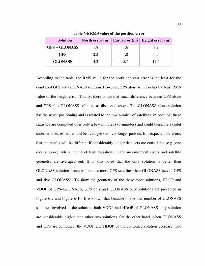
133
Table 6-6 RMS value of the position error
Solution North error (m) East error (m) Height error (m)
GPS + GLONASS 1.8 1.6 7.2
GPS 2.3 1.8 6.5
GLONASS 4.2 5.7 12.5
According to the table, the RMS value for the north and east error is the least for the
combined GPS and GLONASS solution. However, GPS alone solution has the least RMS
value of the height error. Totally, there is not that much difference between GPS alone
and GPS plus GLONASS solution, as discussed above. The GLONASS alone solution
has the worst positioning and is related to the low number of satellites. In addition, these
statistics are computed over only a few minutes (~3 minutes) and could therefore exhibit
short term biases that would be averaged out over longer periods. It is expected therefore,
that the results will be different if considerably longer data sets are considered (e.g., one
day or more), where the short term variations in the measurement errors and satellite
geometry are averaged out. It is also noted that the GPS solution is better than
GLONASS solution because there are more GPS satellites than GLONASS (seven GPS
and five GLONASS). To show the geometry of the these three solutions, HDOP and
VDOP of GPS+GLONASS, GPS only and GLONASS only solutions are presented in
Figure 6-9 and Figure 6-10. It is shown that because of the low number of GLONASS
satellites involved in the solution; both VDOP and HDOP of GLONASS only solution
are considerably higher than other two solutions. On the other hand, when GLONASS
and GPS are combined, the VDOP and HDOP of the combined solution decrease. The

134
steps of changes in DOP values are related to the increase in the number of the satellites
involved in the solution.
508460 508520 508580 5086401
1.2
1.4
1.6
1.8
2
2.2
2.4
2.6
2.8
3
15:14 15:15 15:16 15:17GPS time (sec) and Local time (HH:MM)
VDOP
VD
OP
GPS+GLONASS
GPS
GLONASS
Figure 6-9 VDOP of GPS+GLONASS, GPS only and GLONASS only solutions
508460 508520 508580 5086400.8
1
1.2
1.4
1.6
1.8
2
2.2
2.4
2.6
15:14 15:15 15:16 15:17GPS time (sec) and Local time (HH:MM)
HDOP
HD
OP
GPS+GLONASS
GPS
GLONASS
Figure 6-10 HDOP of GPS+GLONASS, GPS only and GLONASS only solutions
135
Finally, with 20 GLONASS satellites in the constellation in February 2009, more
GLONASS signals can be acquired, tracked and utilized in navigation solution and better
results are predicted.

136
CHAPTER SEVEN: SUMMARY, CONCLUSION, AND RECOMMENDATIONS
7.1 Chapter outline
In this Chapter, the research presented throughout this thesis is summarized. The
conclusions of this research are presented and possible future work in this field of
research is recommended.
7.2 Summary
At the beginning, the GLONASS L1, GLONASS L2 and GPS L1 samples were collected
using three channels of an RF front-end on 10th of October 2008. The antenna used for
this purpose is capable of receiving GPS L1/L2 and GLONASS L1/L2 signals.
The collected samples were acquired using software implemented in Matlab™. This
software was utilized to acquire GPS L1, GLONASS L1 and GLONASS L2 signals.
With the mentioned data set, 10 GPS, six GLONASS L1 and five GLONASS L2 signals
were acquired. Through the acquisition process, the initial tracking information including
initial carrier Doppler frequency and ranging code offset for all the acquired signals were
extracted.
137
After implementing required modifications in GSNRx™, the software was made able to
track GLONASS L1 and GLONASS L2 signals for as many channels as possible.
Acceptable tracking results showed that tracking process has been accomplished
successfully. Moreover, this software was modified in a way that is capable of decoding
GLONASS L1 and GLOANSS L2 navigation message. To verify the GLONASS
software receiver, the navigation solution from this software was compared with the
navigation solution from a commercial receiver. Comparison between the navigation
solutions of the software receiver and the commercial receiver confirmed that the
GLONASS software receiver was working properly. In addition, tracking both L1 and L2
GLONASS signals allowed for the removal of the effect of ionosphere error.
Considering the differences and similarities of GPS and GLONASS systems in addition
to GLONASS L1 and GLONASS L2 signals, necessary modifications was implemented
in the software receiver to provide a GPS plus GLONASS software receiver. The
combined (GPS L1 + GLONASS L1 + GLONASS L2) version of the GSNRx™ is
capable of reading three files containing GPS L1, GLONASS L1 and GLONASS L2
samples, tracking their signals and providing navigation solution.
7.3 Conclusion
Some of the conclusions from this research are presented here:
1. The FFT acquisition algorithm which is commonly used for GPS could also be
used for GLONASS by modification of the relevant parameters. FFT method is
capable of detecting weak signals which is proper for GLONASS L2 signals but
138
still is relatively slow in terms of computation. All the GLONASS signals from
healthy satellites visible during the data collection were acquired by this method.
2. The tracking algorithm applied to GPS signal is applicable to GLONASS L1 and
GLONASS L2 signals as well after updating relevant parameters. The promising
results from Doppler frequency, correlator outputs, C/N0 values, FLI and PLI for
both GLONASS L1 and L2 signals confirmed that the tracking process is working
properly for all the acquired GLONASS L1 and GLONASS L2 signals.
3. A new algorithm (relative to GPS) for decoding GLONASS navigation message
was developed because GPS navigation message structure is completely different
from GLONASS navigation message structure. Following the implementation, the
algorithm was verified by comparing the extracted ephemeris information with
the extracted ephemeris from a commercial receiver.
4. The GLONASS L1-only software receiver is working well. This is confirmed by
comparing the navigation solution from the GLONASS L1-only solution of the
software receiver (GSNRx™) with the navigation solution from NovAtel™
receiver. With a small difference in the RMS value of the positioning error, both
solutions showed similar results in case of north, east and height errors.
5. The GLONASS L2-only software receiver is working well. This is confirmed by
comparing the navigation solution from the GLONASS L1-only and GLONASS
L2-only solutions of GSNRx™. There is a small difference in case of north and
east positioning error but a considerable difference in vertical error which is
related to the rejections of one of the GLONASS L2 signals in some epochs of L2
solution processing.
139
6. Taking the advantage of receiving civilian navigation message on GLONASS L2
signal from GLONASS satellites type M facilitates mitigation of the ionosphere
effect on pseudorange. By implementing ionosphere removal algorithm on the
pseudorange, although the ionosphere error is mitigated, the stochastic errors
increase. As such, the positioning error from the ionosphere-free solution became
worse than the positioning error from L1-only solution. Therefore, there is a
compromise between mitigation of the ionosphere error and increasing stochastic
errors.
7. For a combined GPS and GLONASS software receiver, the similarities of these
two systems helps in tracking the signals and providing navigation solution;
however, the differences must be considered and applied to the software. The
performance of the combined software receiver tracking is checked by comparing
the tracking results of the GPS, GLONASS L1 and GLONASS L2 from the
combined software receiver with the tracking results of GPS-only, GLONASS
L1-only and GLONASS L2-only. The results confirmed that the combined
software receiver is properly tacking three types of signals simultaneously.
8. The navigation solution from the combined software receiver is compared with
the navigation solution from GPS-only and GLONASS-only software receiver.
Because of the small number of GLONASS satellites involved in the navigation
solution relative to the number of GPS satellites and also because of the different
weighting of the systems in the C3NAVG2™ program, the combined navigation
solution tend to follow the navigation solution of GPS-only solution. GLONASS-
140
only solution shows the worse positioning results compared to GPS and
GPS+GLONASS solution because of the small number of GLONASS satellites.
7.4 Recommendations
The following are some of the recommendation for future work on this research:
1. By launching the new generation of GLONASS satellites, GLONASS-K, a third
civil signal (L3) will be added to pervious L1 and L2 signals. As such, expanding
the software receiver to support the new signal is recommended.
2. It is worthy to investigate the performance of the combined software receiver in
kinematics mode. All the data collection set-up during this research was in static
mode. Although no significant differences in performance are expected, it would
still be worth confirming overall performance.
3. Expanding the GPS L1 + GLONASS L1 + GLONASS L2 software receiver in a
way that can track signals from other GNSS systems such as Galileo will provide
the opportunity of tracking more signals and increasing accuracy and reliability
of the navigation solution.
4. Considering the properties of GLONASS ranging codes, the cross-correlation
errors that affect GPS do not affect GLONASS. As such, GLONASS software
receiver can be used for tracking weaker signals.
5. More advanced architectures such as vector tracking and/or ultra-tight integration
with inertial sensors can be applied.
141
REFERENCES
Bao, J., and Y. Tsui (2000a) Fundamentals of Global Positioning System Receivers: a
Software Approach, John Wiley & Sons, Inc., pp.4
Bao, J. and Y. Tsui (2000b) Fundamentals of Global Positioning System Receivers: a
Software Approach, John Wiley & Sons, Inc., pp. 133
Bartenev V., V.E. Kosenko, V.D. Zvonar, V.E. Chebotaryov (2005) “Space vehicle
GLONASS-M. Peculiarities of goal designing,” 10th International Conference on System
Analysis, Controlling and Navigation, Eupatoria, 3-10 July
Bazlov, Y., V.F. Galazin, B.L. Kaplan, V.G. Maksimov, V.P. Rogozin (2006) GLONASS
to GPS: a new coordinate transformation, GPS world, January, Vol. 10, No. 1, pp.54-58
Beser, J., and J. Danaher (1993) “The 3S Navigation R-100 Family of Integrated
GPS/GLONASS Receivers: Description and Performance Results,” in the Proceedings of
Institute of Navigation National Technical Meeting, 20-22 January, San Francisco CA,
pp.25-45
Cannon, M.E. (2007) Satellite Positioning, ENGO 465 Lecture Notes, Department of
Geomatics Engineering, The University of Calgary, Chapter 6, pp.204

142
CDDIS (2008) NASA’s Archive of Geodesy Data, http://cddis.nasa.gov/
gnss_datasum.html, last access 10 February 2009
Chachis, G.C (2001) “Navigation Professional. Public Policy Positions on GLONASS,”
in the Proceedings of Institute of Navigation 57th Annual Meeting/CIGTF 20th Biennial
Guidance Test Symposium, 11-13 June, Albuquerque NM, pp.109-120
Charkhandeh, S., M.G. Petovello and G. Lachapelle (2006) “Performance Testing of a
Real-Time Software-Based GPS Receiver for x86 Processors,” in Proceedings of ION
GNSS, 26-29 September, Forth Worth TX, pp2313- 2320, U.S. Institute of Navigation,
Fairfax VA
Directorate-General Energy and Transport (2008) Official Documents, http://
ec.europa.eu/dgs/energy_transport/galileo/documents/official_en.htm, last accessed 15
January, 2008
Feairheller, S. and R. Clark (2006) Other Satellite Navigation Systems, Understanding
GPS Principles and Applications, E.D. Kaplan and C. J. Hegarty, eds, Norwood, MA,
Artech House, Inc.,Chapter 11
GLONASS ICD (2002), http://www.GLONASS-ianc.rsa.ru, last accessed 3 February,
2008
143
GLONASS.it (2008) GLONASS System, http://www.GLONASS.it, last accessed 30 June,
2008
GLONASS Constellation Status (2009), http://www.glonass-ianc.rsa.ru, last accessed 21
February 2009
GNSS Program Updates (2008), Institute of Navigation Newsletter, Volume 18, Number
1, Spring 2008, pp.12-13
GPS+Reference Manual (2007) GLONASS Overview, www.novatel.com/ Documents/
Manuals/GPS+Reference.pdf, Chapter 5, last accessed 15 January, 2008
Heckler, G.W., and J. L. Garrison (2004) “Architecture of a Reconfigurable Software
Receiver”, in the Proceedings of Institute of Navigation GPS 2004, 21-24 September,
Long Beach CA, pp.947-955, U.S. Institute of Navigation, Fairfax VA
Heinrichs, G., M. Restle, C. Dreischer, and T. Pany (2007) “NavX®-NSR – A Novel
Galileo/GPS Navigation Software Receiver,” in the Proceedings of Institute of
Navigation GNSS, 25-28 September, Fort Worth TX, pp.231-235, U.S. Institute of
Navigation, Fairfax VA

144
Humphreys, T.D., M. L. Psiaki, P.M. Kintner, Jr., and B.M. Ledvina (2006) “GNSS
Receiver Implementation on a DSP: Status, Challenges, and Prospects,” in the
Proceedings of Institute of Navigation GNSS, 26-29 September, Fort Worth TX, pp.2370-
2382, U.S. Institute of Navigation, Fairfax VA
Inside GNSS (2007) China Compass, http://www.insidegnss.com/aboutcompass, last
access January 15, 2008
Kovar, P., F. Vejrazka, L. seidl, and P. Lacmarik (2004) “Implementation of the
GLONASS Signal-Processing Algorithm to the Experimental GNSS Receiver” in the
European Navigation Conference Proceeding, 16-19 May, Rotterdam The Netherlands
Kovar, P., F. Vejrazka, L. seidl, and P. Lacmarik (2005) “GNSS Receiver for GLONASS
signal reception” in IEEE A&E System Magazine, December 2005, pp.21-23
Lachapelle, G. (2007) Advanced GNSS Theory, ENGO 625 Lecture Notes. Deparctment
of Geomatics Engineering, University of Calgary, Chapter 3
Ledvina, B.M, M.L. Psiaki, D.J. Sheinfeld, A.P. Ceruti, S.P. Powel, and P.M. Kintner
(2004) “ A Real-Time GPS Civilian L1/L2 Software Receiver," in the Proceeding Of
Institute of Navigation GPS 2004, 21-24 September, Long beach CA, pp.986-1005, U.S.
Institute of Navigation, Fairfax VA
145
Ledvina, B.M., M. Psiaki, T.E. Humphreys, S.P. Powel, and P.N Kintner (2005) “A Real-
Time Software Receiver Tracking of GPS L2 Civilian Signals Using a Hardware
Simulator,” in the Proceeding of Institute of Navigation GPS 2005, 13-16 September,
Long beach CA, pp.1598-1610, U.S. Institute of Navigation, Fairfax VA
Ledvina, B.M., M. Psiaki, T.E. Humphreys, S.P. Powel, and P.N Kintner (2006) “A Real-
Time Software Receiver for the GPS and Galileo L1 Signal,” in the Proceedings of
Institute of Navigation GPS/GNSS ,26-29 September, Forth Worth TX, pp.2321-2333,
U.S. Institute of Navigation, Fairfax VA
Leick, A. (1995) GPS satellite surveying (2nd ed.), New York NY, John Wiley & Sons
Ma, C., G. Lachapelle, and M.E. Cannon (2004) “Implementation of a Software
Receiver,” in the Proceedings of Institute of Navigation GPS 2004, 21-24 September,
Long Beach CA, pp.882-893, U.S. Institute of Navigation, Fairfax VA
Macchi, F. and M.G. Petovello (2007) “Development of a One Channel Galileo L1
Software Receiver and Testing Using Real Data,” in the Proceedings of Institute of
Navigation GNSS, 25-28 September, Fort Worth TX, pp.2256-2296, U.S. Institute of
Navigation, Fairfax VA
Misra, P. and P. Enge (2001) Global Positioning System Signals, Measurement and
Performance, Lincoln, MA, Ganga-Jamuna Press, pp. 141
146
Mitrikas, V.V., S.G. Revnivykh, and E.V. Bykhanov (1998) "WGS84/PZ90
Transformation Parameters Determination Based on Laser and Ephemeris Long-Term
GLONASS Orbital Data Processing", in the Proceedings of the 11th
International
Workshop on Laser Ranging, Deggendorf, Germany, September 21-25, p. 279
Mumford, P.J, K. Parkinson, and A. Dempster (2006) “The Namuru Open GNSS
Research Receiver ,” in the Proceedings of Institute of Navigation GNSS, 26-29
September, Fort Worth TX, pp.2847-2855, U.S. Institute of Navigation, Fairfax VA
Muthuraman, K., S. K. Shanmugam, and G. Lachapelle (2007) “Evaluation of Data/Pilot
Tracking Algorithms for GPS L2C Signals Using Software Receiver,” in the Proceedings
of Institute of Navigation GNSS, 25-28 September, Fort Worth TX, pp.2499-2509, U.S.
Institute of Navigation, Fairfax VA
NAVIGADGET (2007) Navigation Satellite Wars, http:// www.navigadget.com
/index.php/2007/04/10/navigation-satellite-wars/, last accessed January, 2008
Normark, P.L., and C. Ståhlberg (2005) “Hybrid GPS/Galileo Real-time Software
Receiver, ” in the Proceeding of Institute of Navigation GPS 2005, 13-16 September,
Long beach CA, pp.1906-1613, U.S. Institute of Navigation, Fairfax VA
147
O’Driscoll, C. (2007) Performance Analysis of the Parallel Acquisition of Weak GPS
Signals, PhD Thesis, National University of Ireland, (Available at
http://plan.geomatics.ucalgary.ca/)
Parkinson, B. W. (1996) Introduction and Heritage of NAVSTAR, the Global Positioning
System; Global Positioning System: Theory And Application, .B. Parkinson and J. J.
Spilker Jr., eds., volume 1, American Institute of Aeronautics and Astronautics, Inc.,
Washington D.C., USA, Chapter 1
Petovello, M.G., and G. Lachapelle (2006) “An Efficient New Method of Doppler
Removal and Correlation with Application to Software-Based GNSS Receivers,” in the
Proceedings of the 19th International Technical Meeting of the Satellite Division of the
Institute of Navigation ION GNSS, September 26 - 29, Fort Worth, Texas, pp.2407–2417
Petovello, M.G. and C. O’Driscoll (2007) GSNRx™ Algorithm design Document,
Position, Location And Navigation (PLAN) Group, Department of Geomatics
Engineering, The University of Calgary, Canada
Petovello, M.G., C. O’Driscoll, G. Lachapelle, D. Borio, and H. Murtaza (2008)
“Architecture and Benefits of an Advanced GNSS Software Receiver,” in the Proceeding
of International Symposium on GPS/GNSS 2008, November 11-14, 2008, Tokyo, Japan
148
Polischuk, G. and S. Revnivykh (2004) Status and Development of GLONASS, available
at www.sciencedirect.com, last access April, 2008
Psiaki, M.L.(2001)“Block acquisition of weak GPS signals in a software receiver,” In the
Proceedings of the 14th International Technical Meeting of the Satellite Division of the
Institute of Navigation GPS 2001, 11-14 September, pp. 2838–2870. Institute of
Navigation, Salt Lake City, Utah,
Rambo, J.C. (1989) “Receiver Processing Software Design of the Rockwell International
DoD Standard GPS Receivers,” in the proceedings of the Institute of Navigation GPS 89,
27-29 September, Colorado Springs, CO
Ray, J.K. (2007) Advanced GNSS Receiver Technology, ENGO 638 Course Notes,
Department of Geomatics Engineering, University of Calgary, Canada, pp.54-83
Revnivykh, S.G. (2007) “GLONASS Status, Development and Application,”
International Committee on Global Navigation Satellite System (ICG) Second meeting,
September 4-7, 2007, Bangalore, India
Ryan, S. (2002) Augmentation of DGPS for Marine Navigation, PhD thesis, Department
of Geomatics Engineering, University of Calgary, Canada, Chapter seven (Available at
http://plan.geomatics.ucalgary.ca)
149
Satellite on the net (2008) Launch Schedule, www.satelliteonthenet.co.uk , last access
April 2008
Sharawi, M.S., and O.V. Korniyenko (2007) “Software Defined Radios: A Software GPS
Receiver Example,” in IEEE/ACS International Conference on Computer Systems and
Applications, 13-16 May, Amman, Jordan, pp.562 – 565
Skone, S., G. Lachapelle, D. Yao, W. Yu and R. Watson (2005) “Investigating the Impact
of Ionospheric Scintillation using a GPS Software Receiver,” in the Proceedings of
Institute of Navigation GNSS 2005, 13-16 September, Long Beach CA, U.S. Institute of
Navigation, Fairfax VA
Spelat, M., F. Dovis, G. Girau, and P. Mulassano (2006) “ A Flexible FPGA/DSP Board
for GNSS Receivers Design ” , appears in Research in Microelectronics and Electronics
2006 Ph. D., Otranto, pp.77-80
Spilker J.J. Jr., and B.W. Parkinson (1996) Overview of GPS Operation and Design, B.
Parkinson and J. J. Spilker Jr., eds., Global Positioning System: Theory And Applications,
volume 1, Chapter 2, American Institute of Aeronautics and Astronautics, Inc.,
Washington D.C., USA.
Spilker, J.J., Jr. (1977), Digital communication by Satellite, Prentice Hall, Englewood
Cliffs, NJ, Chapter 12, pp.347-357
150
Tomatis, A., F. Dovis, M. Pini, and M. Fantino (2007) “ITACA: a Scientific GNSS
Software Receiver for Innovation Creation and Testing,” in theProceedings of Institute of
Navigation GNSS, 25-28 September, Fort Worth TX, pp.2723-2730, U.S. Institute of
Navigation, Fairfax VA
Van Dierendonck, A.J. (1995) GPS Receivers, Global Positioning System: Theory and
Application, B.W. Parkinson and J.J. Spilker, Jr., volume 1, American Institute of
Aeronautics and Astronautics, Chapter 8
Ward, P.W., J.W. Betz and C.J. Hegarty (2006) Satellite Signal Acquisition, Tracking,
and Data Demodulation, Understanding GPS Principles and Applications, E. D. Kaplan
and C.J. Hegarty, Norwood, MA, Artech House, Chapter 5
Won, J., P. Thomas, and B. Eissfeller (2006) “Design of a Unified MLE Tracking for
GPS/Galileo Software Receivers,” in the Proceedings of Institute of Navigation GNSS,
26-29 September, Fort Worth TX, pp.2396-2406, U.S. Institute of Navigation, Fairfax
VA
Zheng, B. and G. Lachapelle (2005) “GPS Software Enhancements for Indoor Use,” in
the Proceedings of Institute of Navigation GPS 2005, Long Beach CA, 13-16 September,
U.S. Institute of Navigation, Fairfax VA
151
Zinoviev, A.E (2005) “Using GLONASS in Combined GNSS Receivers: Current Status,”
in the Proceedings of Institute of Navigation GPS/GNSS, 13-16 September 2005, Long
Beach CA, pp.1046-1057, U.S. Institute of Navigation, Fairfax VA