Embed Size (px)
Citation preview
Multiband and Small Size Fractal Square Koch Antenna Design for
UHF/SHF Application
LM
Dilara Khatun
k
A project submitted
in partial fulfillment of the requirement for the degree of M.Sc. in
Electrical and Electronic Engineering
ri - Ur
E..r,•k& J9
Khulna University of Engineering & Technology
'I Khulna 920300, Bangladesh
October 2013
Declaration
This is to certify that the project work entitled "Multiband and Small Size Fractal Square
Koch Antenna Design for UHF/SHF Application" has been carried out by DILARA
KHATUN in the Department of Electrical and Electronic Engineering, Khulna University
of Engineering & Technology, Khulna, Bangladesh. The above project work or any part of
this work has not been submitted anywhere for the award of any degree or diploma.
L3
Signature of Supervisor Vthuci hct
Signature of Candidate (3, I 0 20 I 3

Approval
This is to certify that the project work submitted by DILARA KHATUN entitled
Multiband and Small Size Fractal Square Koch Antenna Design for UHF/SHF
Application" has been approved by the board of examiners for the partial fulfillment of the
requirements for the degree of M.Sc. in the Department of Electrical and Electronic
Engineering, Khulna University of Engineering & Technology, Khulna, Bangladesh in
October, 2013.
BOARD OF EXAMINERS
I.
Prof. Dr. Md. Shahjahan Department of EEE Khulna University of Engineering & Technology
Head Department of EEE Khulna University of Engineering & Technology
Prof. Dr. Md. Abdus Samad Department of EEE Khulna University of Engineering & Technology
4.
Prof. Dr. Md. Nurunnabi Mollah Department of EEE Khulna University of Engineering & Technology
Chairman (Supervisor)
Member
Member
Member
5. _____
Prof. Dr. Md. Maniruzzaman Member Department of ECE Khulna University, Khulna-9208

Acknowledgement I-
It's my pleasure to express the greatest and deepest gratitude to the supreme of the
universe, the almighty Allah, to whom all praises go for enabling me to complete my
project work.
T wuthà like to express my indebtedness to my respected supervisor, Dr. Md. Shahjahan,
Professor, Department of Electrical and Electronic Engineering, Khulna University of
Engineering & Technology, Khulna, for his continuous guidance, keen interest, strong
inspiration, time to time help and constructive criticism to carry on the project work.
Without his guidance, probing questions and limitless support, I wouldn't have completed
this journey.
I also would like to express my humble gratitude to all the respected teachers of EEE
discipline for their effective and fruitful inspiration.
At last but not the least, I am grateful to my parents for their true love. Most importantly,
without their love, continuous support and patience, this project would not have been
possible.
Dilara Khatun
iv
Abstract
There exists various types of antennas for various purposes, but the interest in this area is
increasing day by day. There have been ever growing demands for antenna designs that
possess the highly desirable properties: compact size, low profile, multi-band, wide
bandwidth, high gain, improved SWR etc. Fractal antennas can be used to meet these
demands. This paper represents the analysis and design of multiband square Koch fractal
dipole antenna, where it is shown that as the iterations are increased, the band of
frequencies also increase and the antenna is also compact in size. The designed antenna
has operating frequencies for first iteration are of 496 MHz and 1430 MHz, and for second
iteration are of 460 MHz, 1248 MHz, 1926 MHz and 4390 MHz with acceptable
bandwidth, which has useful applications in U}I1F/SHF. The radiation characteristics,
SWR, reflection-coefficient, input impedance and gain of the proposed antenna are
described with 4NEC2 Software package. Here, the antenna is placed in the XY-plane for
the first iteration and in YZ-plane for the second iteration.
V
Contents
I
MA
Page
Title Page i
Declaration
Approval
Acknowledgement iv
Abstract V
Contents vi
List of Tables ix
List of Figures x
List of Abbreviations xi
Nomenclature xii
Chapter-i Introduction
1.1 Introduction 1
1.2 Objective of the project 2
1.3 Outline of the project 2
Chapter-2 Antenna Theory
2.1 Introduction 3
2.2 Classification of antennas 4
2.2.1 Antenna classification on frequency basis 4
2.2.2 Antenna classification on aperture basis 4
1 Wire antenna 5
Inverted-F antenna 5
2 Horn antenna 6
3 Parabolic antenna 6
4 Microstrip Patch antenna 7
2.2.3 Antenna classification on polarization basis 8
1 Linearly polarized antenna 8
2 Circularly polarized antenna 8
2.2.4 Antenna classification on radiation pattern basis 8
1 Isotropic antenna 8
vi
.41
2 Omnidirectional antenna 9
3 Directional antenna 10
4 Hemispherical antenna 10
2.2.5 Fractal antenna 11
2.3 Antenna properties 11
2.3.1 Operating frequency 12
2.3.2 Wavelength 12
2.3.3 VSWR 12
2.3.4 Return Loss 12
2.3.5 Bandwidth 13
2.3.6 Antenna Radiation Pattern 13
2.3.7 Impedance 14
2.3.8 Radiation Resistance 15
2.3.9 Antenna Efficiency 15
Chapter-3 Fractals and Fractal Antennas
3.1 Introduction 16
3.2 Definition of Fractal 16
3.3 Dimension of Fractal 17
3.4 Fractal Antenna 18
3.5 Features of Fractal Antenna 18
3.5.1 Multibandl Wideband performance 19
3.5.2 Compact Size 19
3.5.3 Cost Effective 20
3.6 Advantages and Disadvantages 20
3.7 Different Fractal Antennas 21
3.7.1 Fractal Wire Antennas 21
1. Koch Fractal 21
Square Koch Fractal 21
Triangular Koch Curve 22
3.7.2 Fractal Patch antennas 23
1. The Sierpinski Triangle 23
VII
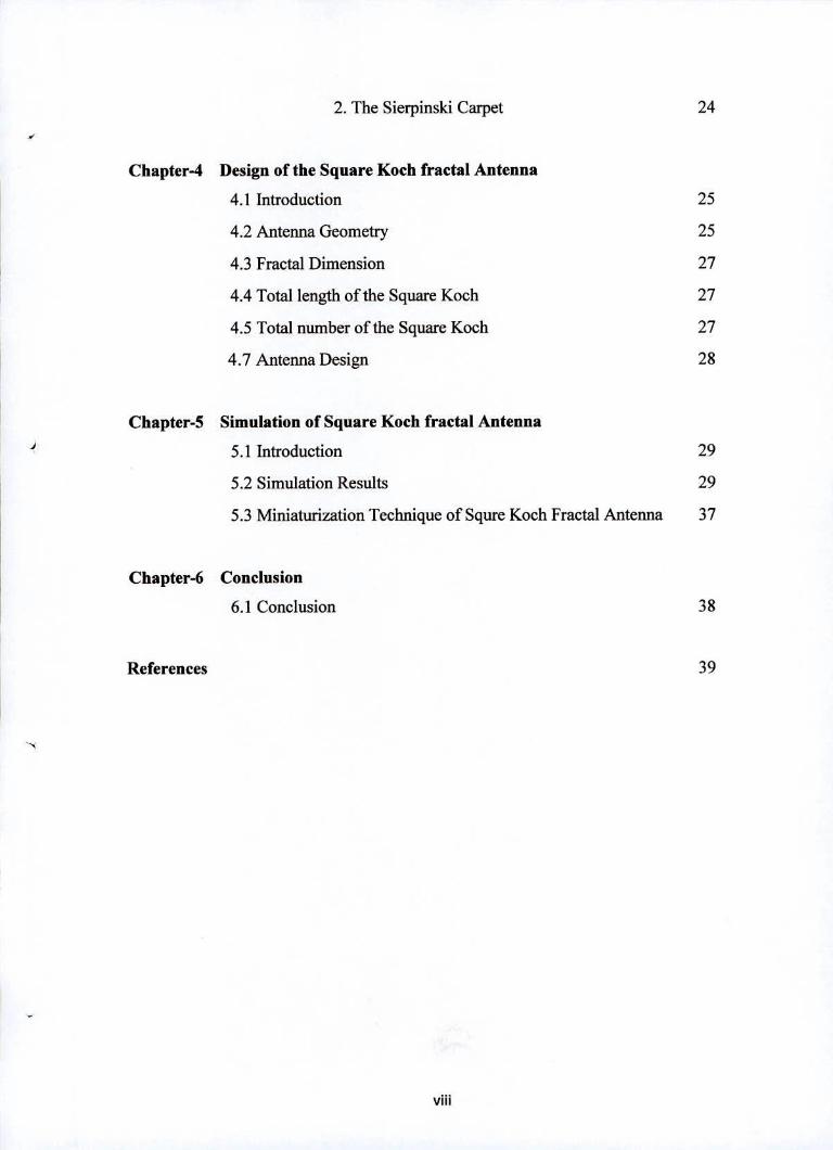
2. The Sierpinski Carpet 24
Chapter4 Design of the Square Koch fractal Antenna
4.1 Introduction 25
4.2 Antenna Geometry 25
4.3 Fractal Dimension 27
4.4 Total length of the Square Koch 27
4.5 Total number of the Square Koch 27
4.7 Antenna Design 28
Chapter-5 Simulation of Square Koch fractal Antenna
5.1 Introduction 29
5.2 Simulation Results 29
5.3 Miniaturization Technique of Squre Koch Fractal Antenna 37
Chapter-6 Conclusion
6.1 Conclusion 38
References 39
VIII
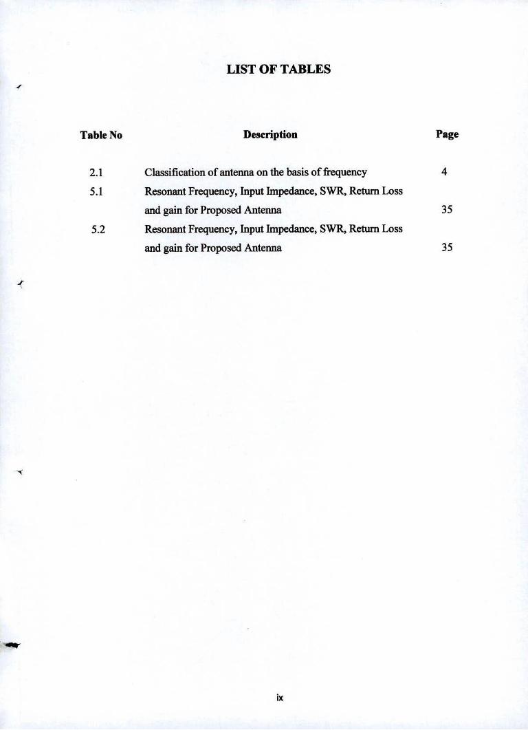
LIST OF TABLES
Table No Description Page
2.1 Classification of antenna on the basis of frequency 4
5.1 Resonant Frequency, Input Impedance, SWR, Return Loss
and gain for Proposed Antenna 35
5.2 Resonant Frequency, Input hnpedance, SWR, Return Loss
and gain for Proposed Antenna 35
Ix
A
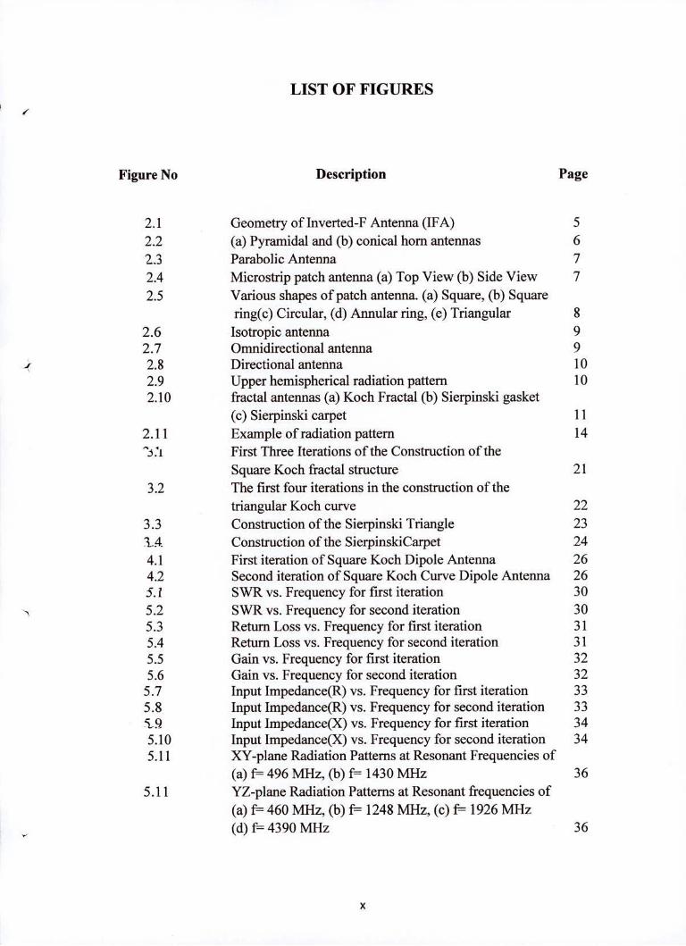
LIST OF FIGURES
Figure No Description Page
2.1 Geometry of Inverted-F Antenna (IFA) 5 2.2 (a) Pyramidal and (b) conical horn antennas 6 2.3 Parabolic Antenna 7 2.4 Microstrip patch antenna (a) Top View (b) Side View 7 2.5 Various shapes of patch antenna. (a) Square, (b) Square
ring(c) Circular, (d) Annular ring, (e) Triangular 8 2.6 Isotropic antenna 9 2.7 Omnidirectional antenna 9 2.8 Directional antenna 10 2.9 Upper hemispherical radiation pattern 10 2.10 fractal antennas (a) Koch Fractal (b) Sierpinski gasket
(c) Sierpinski carpet 11 2.11 Example of radiation pattern 14 'i .i First Three Iterations of the Construction of the
Square Koch fractal structure 21 3.2 The first four iterations in the construction of the
triangular Koch curve 22 3.3 Construction of the Sierpinski Triangle 23 14. Construction of the SierpinskiCarpet 24 4.1 First iteration of Square Koch Dipole Antenna 26 4.2 Second iteration of Square Koch Curve Dipole Antenna 26 5.1 SWR vs. Frequency for first iteration 30 5.2 SWR vs. Frequency for second iteration 30 5.3 Return Loss vs. Frequency for first iteration 31 5.4 Return Loss vs. Frequency for second iteration 31 5.5 Gain vs. Frequency for first iteration 32 5.6 Gain vs. Frequency for second iteration 32 5.7 Input Impedance(R) vs. Frequency for first iteration 33 5.8 Input Impedance(R) vs. Frequency for second iteration 33
Input Impedance(X) vs. Frequency for first iteration 34 5.10 Input Impedance(X) vs. Frequency for second iteration 34 5.11 XY-plane Radiation Patterns at Resonant Frequencies of
(a) f 496 MHz, (b) f= 1430 MHz 36 5.11 YZ-plane Radiation Patterns at Resonant frequencies of
(a) f= 460 MHz, (b) f= 1248 MHz, (c) f= 1926 MHz (d)f4390 MHz 36
I,
x
LIST OF ABBREVIATIONS
IFS Iterated Function System
FBR Front to-Back Ratio
VSWR Voltage Standing Wave Ratio
MOM Methods of Moments
FBW Frequency Bandwidth
MIMO Multi-Input Multi-Output
UHF Ultra High Frequency
SHF Super High Frequency
HPBW Half Power Beamwidth
FNBW First Null Beamwidth
x
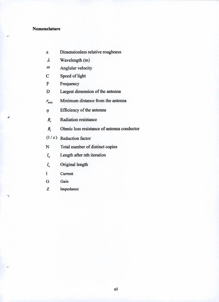
Nomenclature
Dimensionless relative roughness
Wavelength (m)
Anglular velocity
C Speed of light
F Frequency
D Largest dimension of the antenna
rmn Minimum distance from the antenna
77 Efficiency of the antenna
R Radiation resistance
R, Ohmic loss resistance of antenna conductor
(I / ii) Reduction factor
N Total number of distinct copies
l, Length after nth iteration
10 Original length
I Current
G Gain
Z Impedance
XII
CHAPTER 1
Introduction
1.1 Introduction
With the advance of wireless communication; wideband, multiband and low profile
antennas are in great demand for both commercial and military applications. This has
initiated antenna research in various directions, one of which uses fractal shaped antenna
1 elements [1]. Several fractal geometries have been introduced for antenna applications
with varying degrees of success in improving antenna characteristics. Some of these
geometries have been particularly useful in reducing the size of the antenna, while other
designs aim at incorporating multi-band characteristics [2].
The term 'Fractal' [4] was first introduced by Benoit Mandelbrot to classify the structure
whose dimensions were not whole numbers. Mandelbrot defined fractal as a fragmented
geometric shape that can be subdivided in parts, each of which is a reduced-size copy of
the whole. In the mathematics, fractals are a class of complex geometric shapes commonly
exhibit the property of self-similarity, such that small portion of it can be viewed as a
reduced scale replica of the whole.
Since the pioneering work of Mandelbrot and others, a wide variety of applications for
fractals has been found in many branches of science and engineering. One of the most
promising areas of fractal is its application to antenna theory and design [3]. These are low
profile antennas with moderate gain and can be made operative at multiple frequency
bands and hence are multi-functional.
The Simplest example of antenna using fractal geometry is given by the Swedish
mathematician H. von Koch in 1904, which is known as Koch fractal.
1

In this project a wire square Koch fractal antenna is designed based on the first and second
iterations of square Koch curve geometry [4] .Here, it is shown that as the iterations are
increased, the band of frequencies also increase and the antenna is also compact in size
[5].
1.2 Objective of the Project
The main purposes of the project work are given below:
To design the multiband and miniaturized [24] square Koch fractal antenna.
To show that as the iterations are increased, the band of frequencies also -d
increases.
To plot Return loss versus frequency, SWR versus frequency, Gain versus
frequency, Input Impedance versus frequency and radiation pattern of
square Koch fractal antenna.
1.3 Outline of the Project
Chapter 1 explains the introduction of the project and describes the objective of this
project.
Chapter 2 discusses the different types of antennas and antenna properties.
Chapter 3 discusses the fundamental concepts of fractal, fractal dimension, advantages and
disadvantages of fractal antenna, features of fractal antenna, different types of fractal
antennas, application of fractal antenna etc.
Chapter 4 discusses the design of square Koch fractal antenna and antenna geometry of the
proposed antenna.
Chapter 5 presents the simulated result of square Koch fractal antenna.
Chapter 6 highlights the overall conclusion of the project.
2
CHAPTER 2
Antenna Theory
2.1 Introduction
An antenna [2] is a transducer designed to transmit or receive radio waves which are a
class of electromagnetic waves. In other words, antennas convert radio frequency
electrical currents into electromagnetic waves and vice versa.
By definition, an antenna is a device used to transform an RF signal, traveling on a
conductor, into an electromagnetic wave in free space. The IEEE Standard (IEEE Std 145-
1983) defmes the antenna or aerial as "a means for radiating or receiving radio waves". In
other words it is a transitional structure between free space and a guiding device that is
made to efficiently radiate and receive radiated electromagnetic waves. Antennas are
commonly used in radio, television broadcasting, cell phones, radar, and other systems
involving the use of electromagnetic waves.
In some sense the first antenna dates from 1887, when Heinrich Hertz designed brilliant
set of wireless experiments to test James Clerk Maxwell's hypothesis. Hertz used a flat
dipole for a transmitting antenna and a single turn loop for a receiving antenna. For the
next fifty years antenna technology was based on radiating elements configured out of
wires and generally supported by wooden poles. These "wire "antennas were the mainstay
of the radio pioneers, including: (1) Galileo Marconi, (2) Edwin Howard Armstrong and
(3) Lee deforest. Each of these engineers has been called the Father of the Radio. The first
generation antennas were narrowband and were often used to increase directivity.
Development of the array culminated in the work of Hidetsu Yagi and Shintaro Uda
(1926). During this period broadband antennas were also developed. The Yagi-Uda
antenna remained king until after the war. Then during the 1950s and 1960s research at the
University of Illinois culminated in the development of a class of antennas that became
3
11
known as frequency independent. These have performance that is periodic in a logarithmic
fashion and have come to be known as "log-periodic" antennas. In recent years, fractal
antennas are coming out smaller, cheaper and more reliable.
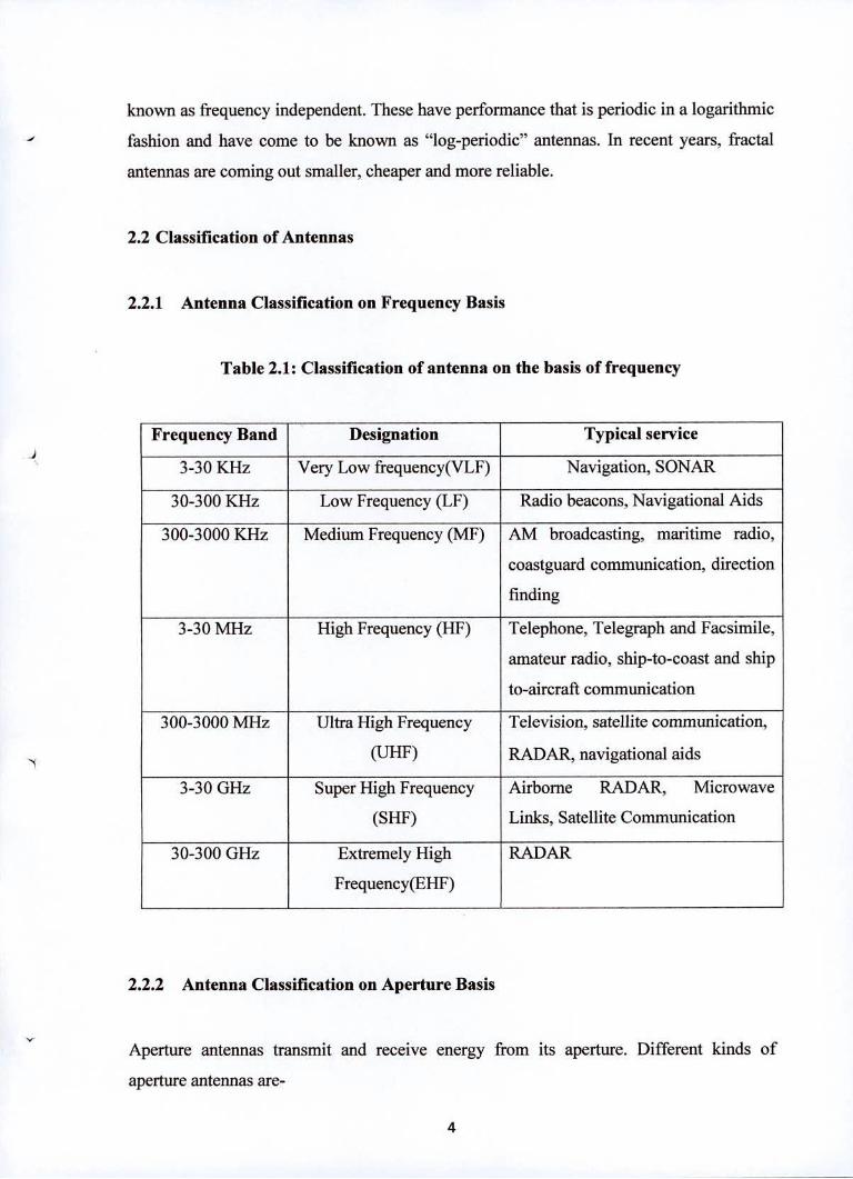
2.2 Classification of Antennas
2.2.1 Antenna Classification on Frequency Basis
Table 2.1: Classification of antenna on the basis of frequency
Frequency Band Designation Typical service
3-30 KHz Very Low frequency(VLF) Navigation, SONAR
30-300 KHz Low Frequency (LF) Radio beacons, Navigational Aids
300-3000 KHz Medium Frequency (MF) AM broadcasting, maritime radio,
coastguard communication, direction
finding
3-30 MHz High Frequency (HF) Telephone, Telegraph and Facsimile,
amateur radio, ship-to-coast and ship
to-aircraft communication
300-3000 MHz Ultra High Frequency Television, satellite communication,
(UHF) RADAR, navigational aids
3-30 GHz Super High Frequency Airborne RADAR, Microwave
(SHF) Links, Satellite Communication
30-300 GHz Extremely High RADAR
Frequency(EHF)
2.2.2 Antenna Classification on Aperture Basis
Aperture antennas transmit and receive energy from its aperture. Different kinds of
aperture antennas are-
4
Wire antenna
Horn antenna
Parabolic antenna
Microstrip patch antenna
1. Wire Antenna
A wire antenna is simply a straight wire of length 2/2 (dipole antenna) and 2/4
(monopole antenna), where 2 is the transmitted signal wavelength. A wire antenna can be
a loop antenna such as circular loop, rectangular loop etc. Basically all vertical radiators
are come into wire antenna categories.
. Inverted-F Antenna
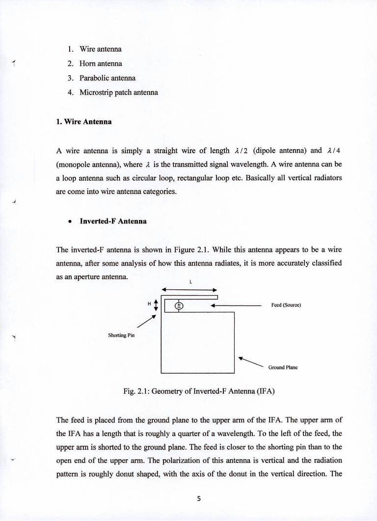
The inverted-F antenna is shown in Figure 2.1. While this antenna appears to be a wire
antenna, after some analysis of how this antenna radiates, it is more accurately classified
as an aperture antenna. L
4
Hj 4 Feed (Source)
7 Shorting Pin
Ground Plane
Fig. 2.1: Geometry of Inverted-F Antenna (IFA)
The feed is placed from the ground plane to the upper arm of the IFA. The upper arm of
the IFA has a length that is roughly a quarter of a wavelength. To the left of the feed, the
upper arm is shorted to the ground plane. The feed is closer to the shorting pin than to the
open end of the upper arm. The polarization of this antenna is vertical and the radiation
pattern is roughly donut shaped, with the axis of the donut in the vertical direction. The
ground plane should be at least as wide as the IFA length (L), and the ground plane should
-d be at least lambdal4 in height. If the height of the ground plane is smaller, the bandwidth
and efficiency will decrease. The height of the IFA (H) should be a small fraction of a
wavelength.
Horn Antenna
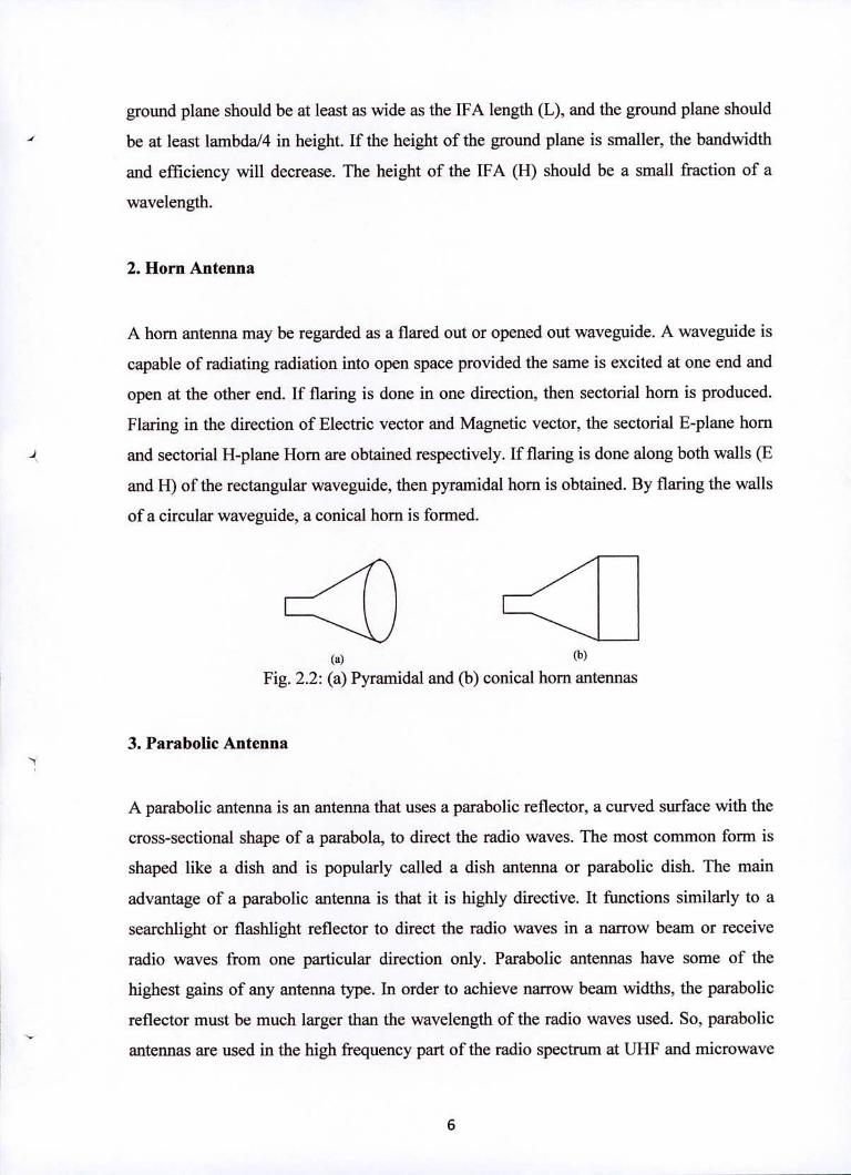
A horn antenna may be regarded as a flared out or opened out waveguide. A waveguide is
capable of radiating radiation into open space provided the same is excited at one end and
open at the other end. If flaring is done in one direction, then sectorial horn is produced.
Flaring in the direction of Electric vector and Magnetic vector, the sectorial E-plane horn
J and sectorial H-plane Horn are obtained respectively. If flaring is done along both walls (E
and H) of the rectangular waveguide, then pyramidal horn is obtained. By flaring the walls
of a circular waveguide, a conical horn is formed.
(a) (b)
Fig. 2.2: (a) Pyramidal and (b) conical horn antennas
Parabolic Antenna
A parabolic antenna is an antenna that uses a parabolic reflector, a curved surface with the
cross-sectional shape of a parabola, to direct the radio waves. The most common form is
shaped like a dish and is popularly called a dish antenna or parabolic dish. The main
advantage of a parabolic antenna is that it is highly directive. It functions similarly to a
searchlight or flashlight reflector to direct the radio waves in a narrow beam or receive
radio waves from one particular direction only. Parabolic antennas have some of the
highest gains of any antenna type. In order to achieve narrow beam widths, the parabolic
reflector must be much larger than the wavelength of the radio waves used. So, parabolic
antennas are used in the high frequency part of the radio spectrum at UHF and microwave
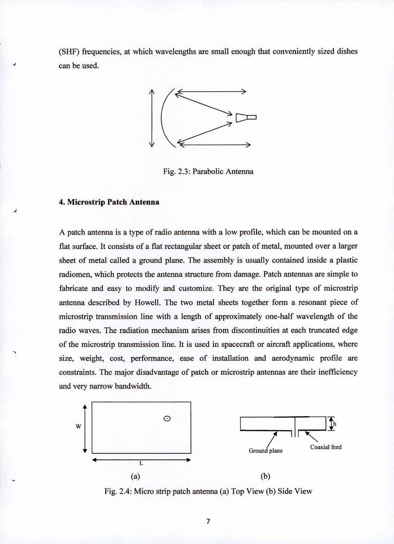
(SHF) frequencies, at which wavelengths are small enough that conveniently sized dishes .1 can be used.
Fig. 2.3: Parabolic Antenna
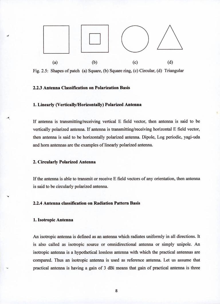
4. Microstrip Patch Antenna -J
A patch antenna is a type of radio antenna with a low profile, which can be mounted on a
flat surface. It consists of a flat rectangular sheet or patch of metal, mounted over a larger
sheet of metal called a ground plane. The assembly is usually contained inside a plastic
radiomen, which protects the antenna structure from damage. Patch antennas are simple to
fabricate and easy to modify and customize. They are the original type of microstrip
antenna described by Howell. The two metal sheets together form a resonant piece of
microstrip transmission line with a length of approximately one-half wavelength of the
radio waves. The radiation mechanism arises from discontinuities at each truncated edge
of the microstrip transmission line. It is used in spacecraft or aircraft applications, where
size, weight, cost, performance, ease of installation and aerodynamic profile are
constraints. The major disadvantage of patch or microstrip antennas are their inefficiency
and very narrow bandwidth.
WI
MO
Ground plane Coaxial feed
L 10
(a) (b)
Fig. 2.4: Micro strip patch antenna (a) Top View (b) Side View
7
-d
In CA (a) (b) (c) (d)
Fig. 2.5: Shapes of patch (a) Square, (b) Square ring, (c) Circular, (d) Triangular
2.2.3 Antenna Classification on Polarization Basis
Linearly (Vertically/Horizontally) Polarized Antenna
If antenna is transmitting/receiving vertical E field vector, then antenna is said to be
vertically polarized antenna. If antenna is transmitting/receiving horizontal E field vector,
then antenna is said to be horizontally polarized antenna. Dipole, Log periodic, yagi-uda
and horn antennas are the examples of linearly polarized antenna.
Circularly Polarized Antenna
If the antenna is able to transmit or receive E field vectors of any orientation, then antenna
is said to be circularly polarized antenna.
2.2.4 Antenna classification on Radiation Pattern Basis
1. Isotropic Antenna
An isotropic antenna is defined as an antenna which radiates uniformly in all directions. It
is also called as isotropic source or omnidirectional antenna or simply unipole. An
isotropic antenna is a hypothetical lossless antenna with which the practical antennas are
compared. Thus an isotropic antenna is used as reference antenna. Let us assume that
practical antenna is having a gain of 3 dBi means that gain of practical antenna is three
-J
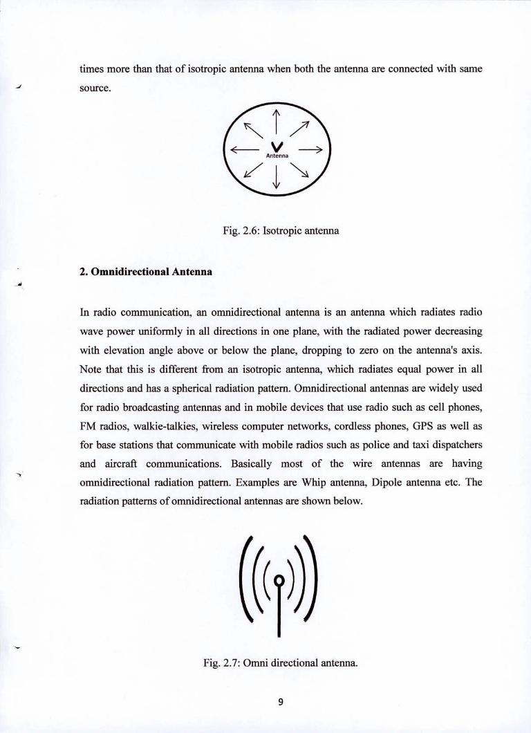
times more than that of isotropic antenna when both the antenna are connected with same
-I source.
Antenna
Fig. 2.6: Isotropic antenna
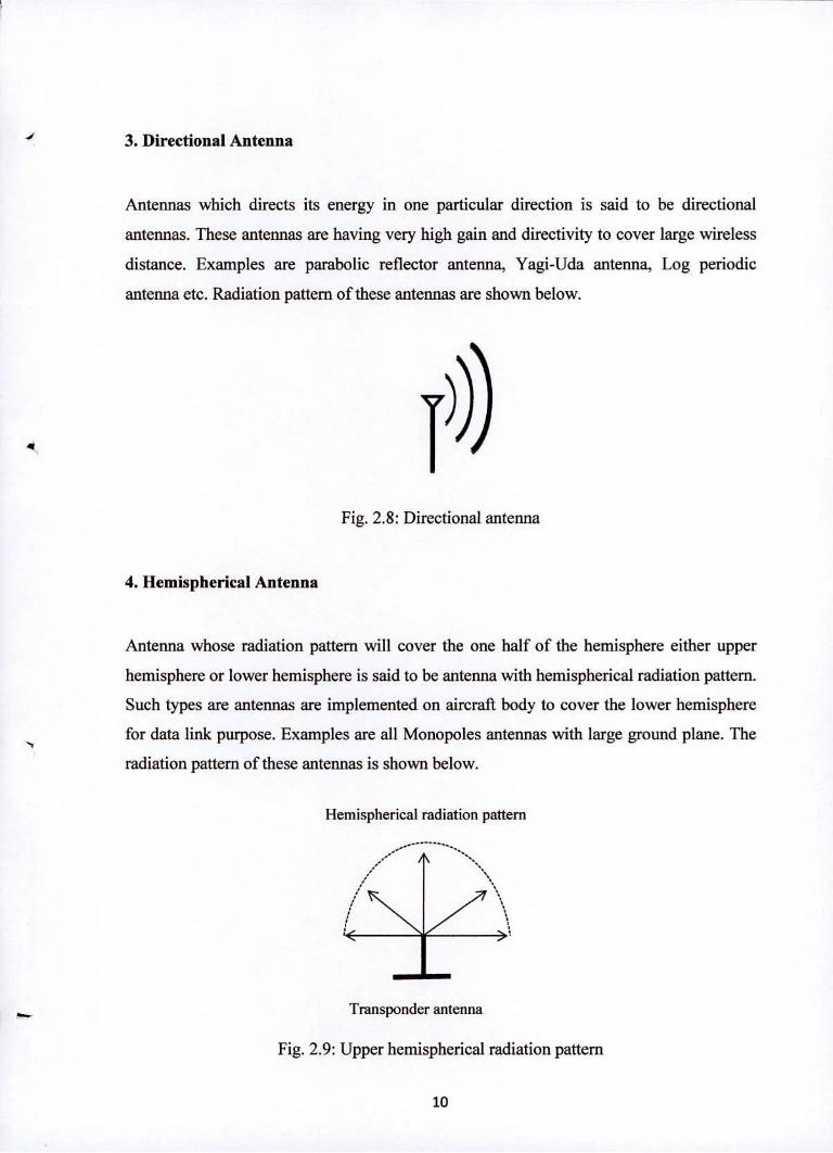
2. Omnidirectional Antenna
In radio communication, an omnidirectional antenna is an antenna which radiates radio
wave power uniformly in all directions in one plane, with the radiated power decreasing
with elevation angle above or below the plane, dropping to zero on the antenna's axis.
Note that this is different from an isotropic antenna, which radiates equal power in all
directions and has a spherical radiation pattern. Omnidirectional antennas are widely used
for radio broadcasting antennas and in mobile devices that use radio such as cell phones,
FM radios, walkie-talkies, wireless computer networks, cordless phones, GPS as well as
for base stations that communicate with mobile radios such as police and taxi dispatchers
and aircraft communications. Basically most of the wire antennas are having
omnidirectional radiation pattern. Examples are Whip antenna, Dipole antenna etc. The
radiation patterns of omnidirectional antennas are shown below.
Fig. 2.7: Omni directional antenna.
ft-
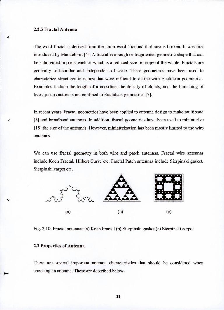
.41 3. Directional Antenna
Antennas which directs its energy in one particular direction is said to be directional
antennas. These antennas are having very high gain and directivity to cover large wireless
distance. Examples are parabolic reflector antenna, Yagi-Uda antenna, Log periodic
antenna etc. Radiation pattern of these antennas are shown below.
4
Fig. 2.8: Directional antenna
4. Hemispherical Antenna
Antenna whose radiation pattern will cover the one half of the hemisphere either upper
hemisphere or lower hemisphere is said to be antenna with hemispherical radiation pattern.
Such types are antennas are implemented on aircraft body to cover the lower hemisphere
11 for data link purpose. Examples are all Monopoles antennas with large ground plane. The
radiation pattern of these antennas is shown below.
Hemispherical radiation pattern
Transponder antenna
Fig. 2.9: Upper hemispherical radiation pattern
10
2.2.5 Fractal Antenna
I
The word fractal is derived from the Latin word 'fractus' that means broken. It was first
introduced by Mandeibrot [4]. A fractal is a rough or fragmented geometric shape that can
be subdivided in parts, each of which is a reduced-size [6] copy of the whole. Fractals are
generally self-similar and independent of scale. These geometries have been used to
characterize structures in nature that were difficult to define with Euclidean geometries.
Examples include the length of a coastline, the density of clouds, and the branching of
trees, just as nature is not confined to Euclidean geometries [7].
In recent years, Fractal geometries have been applied to antenna design to make multiband
) [8] and broadband antennas. In addition, fractal geometries have been used to miniaturize
[15] the size of the antennas. However, miniaturization has been mostly limited to the wire
antennas.
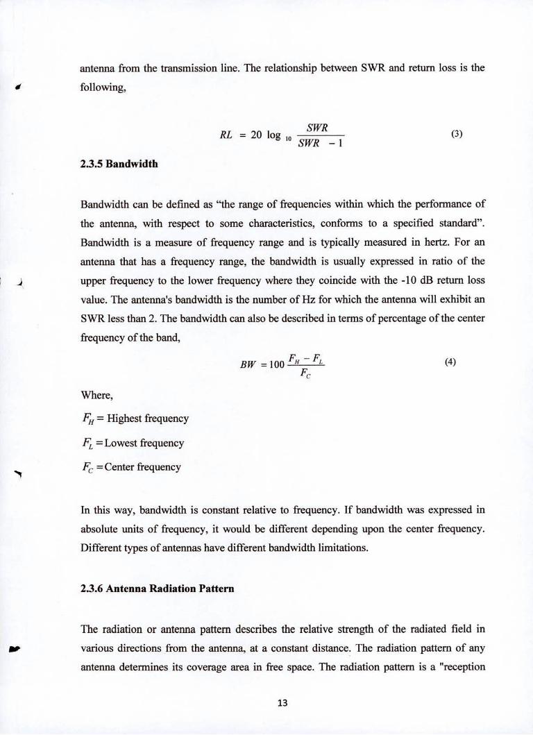
We can use fractal geometry in both wire and patch antennas. Fractal wire antennas
include Koch Fractal, Hilbert Curve etc. Fractal Patch antennas include Sierpinski gasket,
Sierpinski carpet etc.
(a) (b) (c)
Fig. 2.10: Fractal antennas (a) Koch Fractal (b) Sierpinski gasket (c) Sierpinski carpet
2.3 Properties of Antenna
There are several important antenna characteristics that should be considered when
choosing an antenna. These are described below-
11

2.3.1 Operating Frequency
PA
The operating frequency is the frequency range through which the antenna will meet all
functional specifications. It depends on the structure of the antenna in which each antenna
types has its own characteristic towards a certain range of frequency. The operating
frequency can be tuned by adjusting the electrical length of the antenna.
2.3.2 Wavelength
We often refer to antenna size relative to wavelength. For example, a half-wave dipole,
which is approximately a half-wavelength long. Wavelength is the distance that a radio
wave will travel during one cycle. The formula for wavelength is-
2 =
f (1)
Where,
2 = wavelength
C = speed of light
f = frequency
2.3.3 VSWR
VSWR determines the matching properties of antenna. It indicates that how much
efficiently antenna is transmitting/receiving electromagnetic wave over particular band of
frequencies. The VSWR is given by,
VSWR = 1+sII (2)
2.3.4 Return Loss
The return loss is another way of expressing mismatch. It is a logarithmic ratio measured
in dB that compares the power reflected by the antenna to the power that is fed into the
12
antenna from the transmission line. The relationship between SWR and return loss is the
I following,
RL = 20 log 10 SWR
(3) SWR —I
2.3.5 Bandwidth
Bandwidth can be defined as "the range of frequencies within which the performance of
the antenna, with respect to some characteristics, conforms to a specified standard".
Bandwidth is a measure of frequency range and is typically measured in hertz. For an
antenna that has a frequency range, the bandwidth is usually expressed in ratio of the
upper frequency to the lower frequency where they coincide with the -10 dB return loss
value. The antenna's bandwidth is the number of Hz for which the antenna will exhibit an
SWR less than 2. The bandwidth can also be described in terms of percentage of the center
frequency of the band,
BW = 100 F,, - F, (4)
F
Where,
= Highest frequency
Pj = Lowest frequency
F. =Nf
Center frequency
In this way, bandwidth is constant relative to frequency. If bandwidth was expressed in
absolute units of frequency, it would be different depending upon the center frequency.
Different types of antennas have different bandwidth limitations.
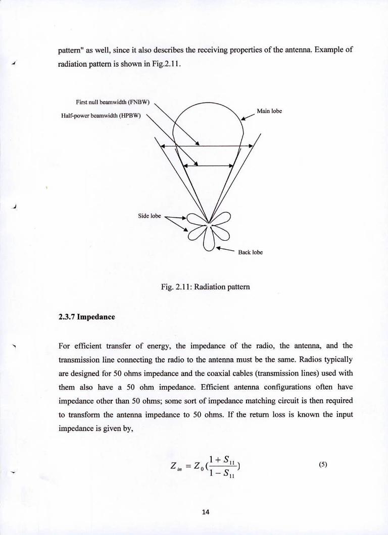
2.3.6 Antenna Radiation Pattern
The radiation or antenna pattern describes the relative strength of the radiated field in
AW various directions from the antenna, at a constant distance. The radiation pattern of any
antenna determines its coverage area in free space. The radiation pattern is a "reception
13
Pli
Half-power beamwidth (IIPBW)
First null beamwidth (FNBW'
Sid
pattern" as well, since it also describes the receiving properties of the antenna. Example of
radiation pattern is shown in Fig.2. 11.
lain lobe
Fig. 2.11: Radiation pattern
2.3.7 Impedance
For efficient transfer of energy, the impedance of the radio, the antenna, and the
transmission line connecting the radio to the antenna must be the same. Radios typically
are designed for 50 ohms impedance and the coaxial cables (transmission lines) used with
them also have a 50 ohm impedance. Efficient antenna configurations often have
impedance other than 50 ohms; some sort of impedance matching circuit is then required
to transfonn the antenna impedance to 50 ohms. If the return loss is known the input
impedance is given by,
z in =Z0( 1+ S11
) (5)
14

2.3.8 Radiation Resistance
4
The radiation resistance is a hypothetical resistance and does not correspond to a real
resistor present in the antenna but to the resistance of space coupled via the beam to the
antenna terminals. Antenna presents impedance at its terminals,
Z A =RA +jX A (6)
Where,
R A = Rr + R1
-J
Rr = Radiation resistance
Ry = Ohmic loss resistance of antenna conductor
2.3.9 Antenna Efficiency (i7 )
The efficiency of antenna is defined as the ratio of power radiated to the total input power
supplied to the antenna and is denoted by i.
Antenna Efficiency, i =Power RadiatedlTotal Input Power.
In terms of resistances,
71=[Rr /(Rr +Ri )]*100 (7)
Where,
R,. = Radiation resistance
14 = Ohmic loss resistance of antenna conductor
15

CHAPTER 3
-I
Fractals and Fractal Antennas
3.1 Introduction
The word fractal is derived from the Latin word 'fractus' that means broken, fragmented,
fractional or irregular. The term 'Fractal' [4] was first introduced by Benoit Mandeibrot to
classify the structure whose dimensions were not whole numbers. A fractal is a rough or
fragmented geometric shape that can be subdivided in parts, each of which is a reduced-
size copy of the whole. Fractals are generally self-similar and independent of scale.
Examples are- length of a coastline, density of clouds and branching of trees, just as nature
is not confined to Euclidean geometries.
The geometry of the fractal antenna encourages its study both as a multiband [9] solution
and also as a small antenna. First, the self similar property to operate in a similar way at
several wavelengths. Second, the space- filling properties of fractals allow fractal shaped
small antennas [19] to better take advantage of the small surrounding space.
3.2 Definition of Fractal
Mandeibrot defines the term fractal in several ways. A fractal is a set for which the
Hausdorif Besicovich dimension strictly exceeds its topological dimension. Every set
having non-integer dimension is a fractal [10]. Fractal objects have some unique
geometrical properties. This are-
A complex structure at any level of magnification.
A non-integer dimension. We know that the dimension of lines, squares,
and cubes are respectively 1, 2, and 3. The dimension of a fractal may be
1.342.
16
Self-similar antenna [14] (which contains many copies of itself at several
scales) to operate in a similar way at several wavelengths. That is, the
antenna should keep similar radiation parameters through several bands.
Space- filling properties [15] of some fractal shapes (the fractal dimension)
might allow fractal shaped small antennas to better take advantage of the
small surrounding space that means an infinite long curve in a finite area.
3.3 Dimension of Fractal
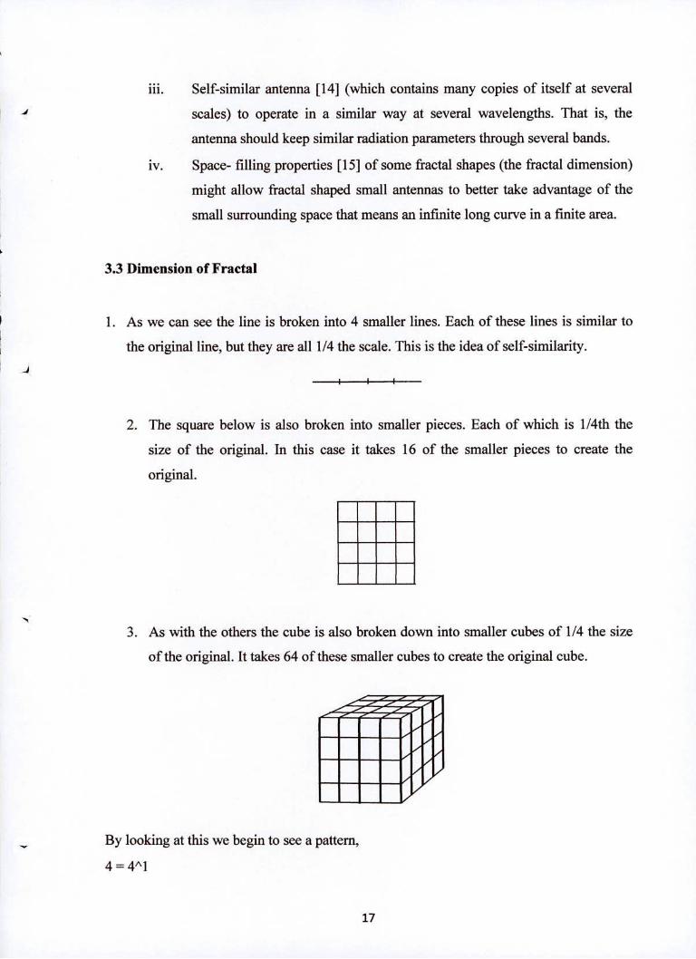
1. As we can see the line is broken into 4 smaller lines. Each of these lines is similar to
the original line, but they are all 1/4 the scale. This is the idea of self-similarity.
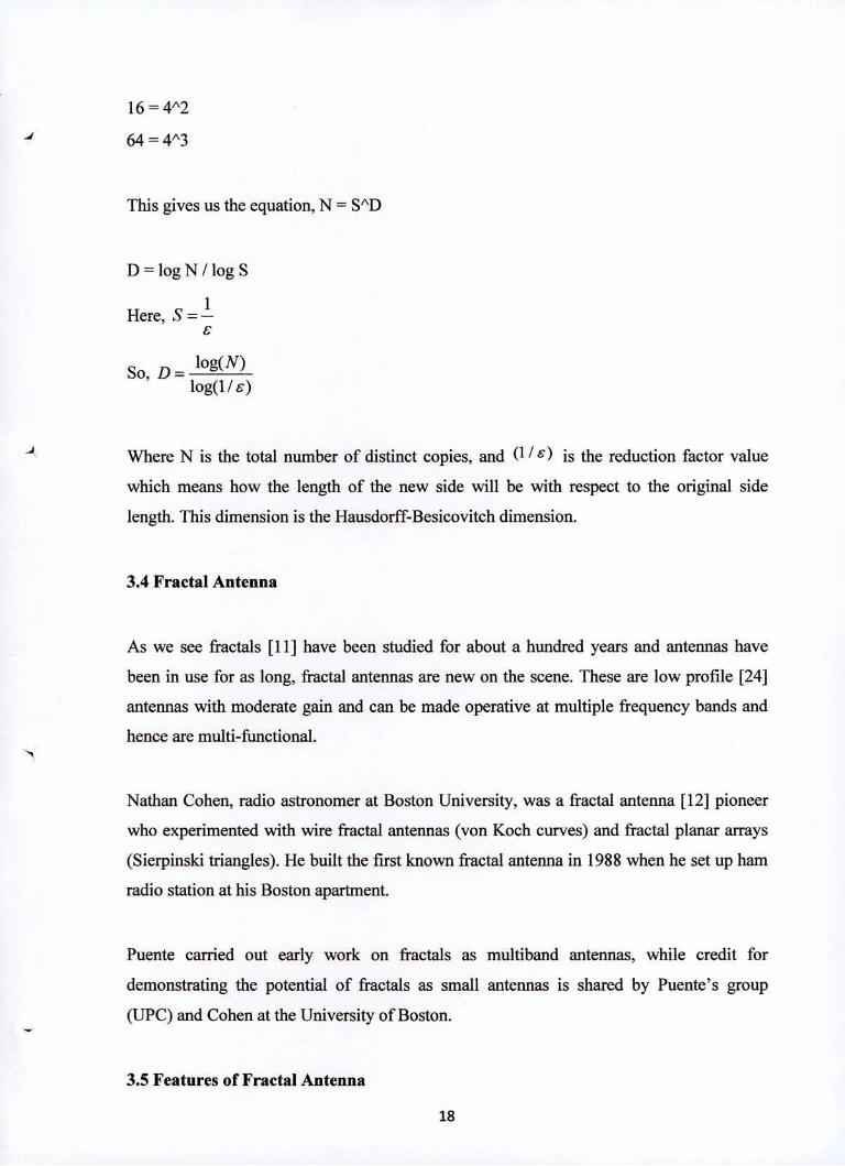
The square below is also broken into smaller pieces. Each of which is 1/4th the
size of the original. In this case it takes 16 of the smaller pieces to create the
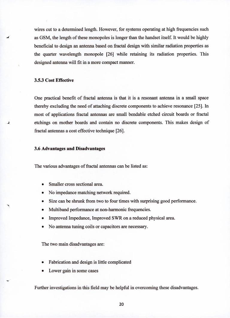
original. No ••ii I-. •.Ii As with the others the cube is also broken down into smaller cubes of 1/4 the size
of the original. It takes 64 of these smaller cubes to create the original cube.
By looking at this we begin to see a pattern,
44A1
17
-I
16 = 4A2
-I 64=4'3
This gives us the equation, N = SAD
D = log N / log S
Here, S =
l So, D=
og(N) log(1/e)
Where N is the total number of distinct copies, and 0 / ) is the reduction factor value
which means how the length of the new side will be with respect to the original side
length. This dimension is the Hausdorff-Besicovitch dimension.
3.4 Fractal Antenna
As we see fractals [11] have been studied for about a hundred years and antennas have
been in use for as long, fractal antennas are new on the scene. These are low profile [24]
antennas with moderate gain and can be made operative at multiple frequency bands and
hence are multi-fimctional.
Nathan Cohen, radio astronomer at Boston University, was a fractal antenna [12] pioneer
who experimented with wire fractal antennas (von Koch curves) and fractal planar arrays
(Sierpinski triangles). He built the first known fractal antenna in 1988 when he set up ham
radio station at his Boston apartment.
Puente carried out early work on fractals as multiband antennas, while credit for
demonstrating the potential of fractals as small antennas is shared by Puente's group
(UPC) and Cohen at the University of Boston.
3.5 Features of Fractal Antenna
18

3.5.1 Multiband/ Wideband Performance
-I
It has been found that for an antenna, to work well for all frequencies, it should be:
Symmetrical: This means that the figure looks the same as its mirror image.
. Self-similar: This means that parts of the figure are small copies of the whole
figure.
These two properties are very common for fractals and thus make fractals [13] ideal for
design of wideband and multiband antennas [16].
Application:
In modem wireless communications more and more systems are introduced which
integrate many technologies and are often required to operate at multiple frequency bands.
Examples of systems using a multi-band antenna are varieties of common wireless
networking cards used in laptop computers. These can communicate on 802.11 b networks
at 2.4 GHz and 802.1 Ig networks at 5 GHz.
3.5.2 Compact Size
Another requirement by the compact wireless systems for antenna design is the compact
size. The fractional dimension and space filling property of fractal shapes allow the fractal
shaped antennas to utilize the small surrounding space effectively [19]. This also
overcomes the limitation of performance of small classical antennas.
Application:
The fractal antenna technology can be applied to cellular handsets. Because fractal antenna
is more compact, it fit more easily in the receiver package. Currently, many cellular
handsets use quarter wavelength monopoles which are essentially sections of radiating
19
wires cut to a determined length. However, for systems operating at high frequencies such
as GSM, the length of these monopoles is longer than the handset itself. It would be highly
beneficial to design an antenna based on fractal design with similar radiation properties as
the quarter wavelength monopole [26] while retaining its radiation properties. This
designed antenna will fit in a more compact manner.
3.5.3 Cost Effective
One practical benefit of fractal antenna is that it is a resonant antenna in a small space
thereby excluding the need of attaching discrete components to achieve resonance [25]. In
most of applications fractal antennas are small bendable etched circuit boards or fractal
etchings on mother boards and contain no discrete components. This makes design of
fractal antennas a cost effective technique [26].
3.6 Advantages and Disadvantages
The various advantages of fractal antennas can be listed as:
. Smaller cross sectional area.
No impedance matching network required.
. Size can be shrunk from two to four times with surprising good performance.
Multiband performance at non-harmonic frequencies.
. Improved Impedance, Improved SWR on a reduced physical area.
. No antenna tuning coils or capacitors are necessary.
The two main disadvantages are:
Fabrication and design is little complicated
• Lower gain in some cases
Further investigations in this field may be helpflil in overcoming these disadvantages.
20
3.7 Different Fractal Antennas
Fractal antennas can take on various shapes and forms depending on the different fractal
geometries. Some of the different types of fractal antennas are:
3.7.1 Fractal Wire Antennas
1. Koch Fractal
Square Koch Fractal
Construction
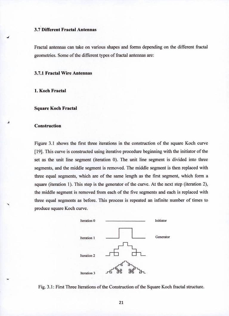
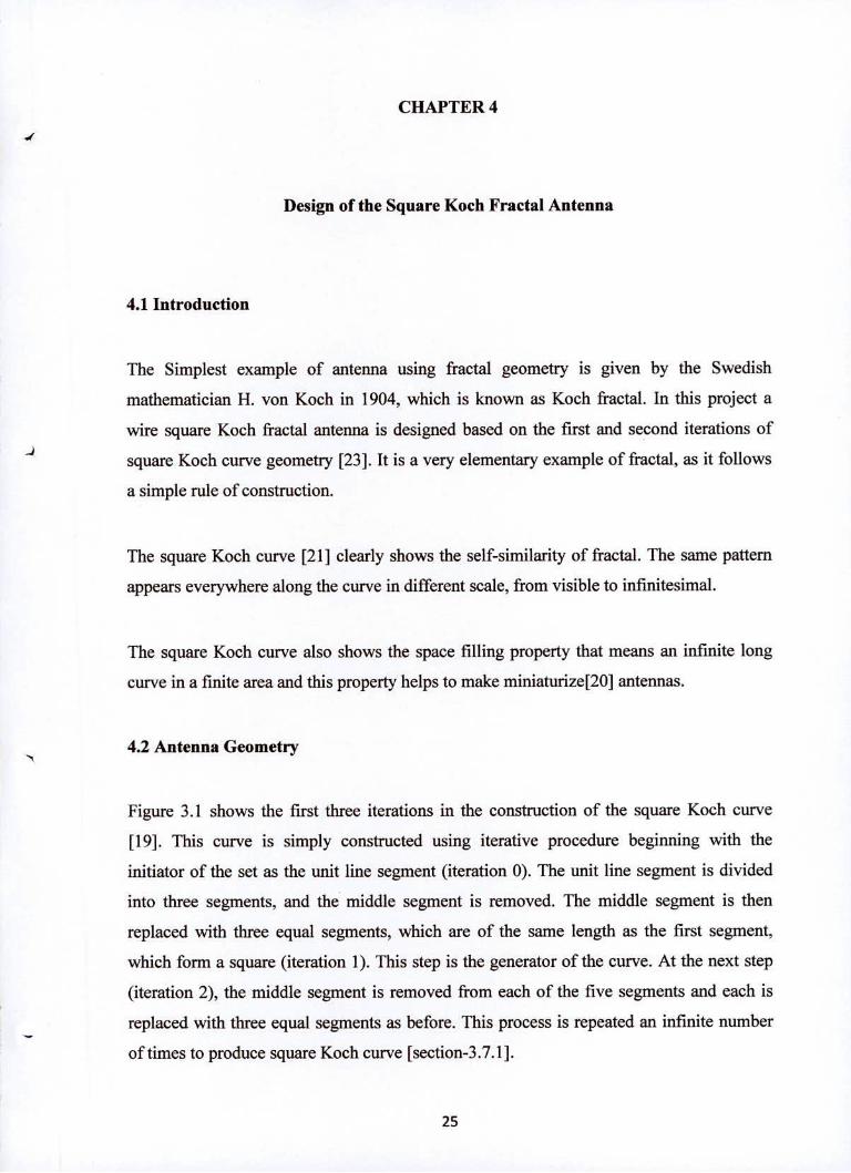
Figure 3.1 shows the first three iterations in the construction of the square Koch curve
[19]. This curve is constructed using iterative procedure beginning with the initiator of the
set as the unit line segment (iteration 0). The unit line segment is divided into three
segments, and the middle segment is removed. The middle segment is then replaced with
three equal segments, which are of the same length as the first segment, which form a
square (iteration 1). This step is the generator of the curve. At the next step (iteration 2),
the middle segment is removed from each of the five segments and each is replaced with
three equal segments as before. This process is repeated an infinite number of times to
produce square Koch curve.
Iteration 0 Initiator
Iteration I Generator
Iteration 2
Iteration 3
Fig. 3.1: First Three Iterations of the Construction of the Square Koch fractal structure.
21
J

Dimension of Square Koch Fractal
N = 5 (Each segment is replaced by 3 new segments)
s = (Each new segment is one third the length of the previous segment)
s=+=3
d = 12g(5)
= 1.46 log( 3)
Triangular Koch Curve
Construction
Start with a straight line. The straight line is divided into 3 equal parts, and the middle part
is replaced by two linear segments at angles 600 and 1200. Then Repeat the stepsi and 2 to
the four line segments. Further iterations will generate the following curves.
Iteration 0 Initiator
Iteration I Generator
Iteration 2
Iteration 3
Fig. 3.2: The first four iterations in the construction of the triangular Koch curve
Dimension of Triangular Koch Fractal
N =4 (Each segment is replaced by 4 new segments)
22
FA
(Each new segment is one third the length of the previous segment)
s=--=3
d = log( 4)
= 1.26 log( 3)
3.7.2 Fractal Patch antennas
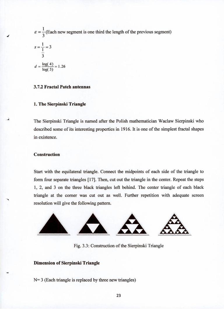
1. The Sierpinski Triangle
The Sierpinski Triangle is named after the Polish mathematician Waclaw Sierpinski who
described some of its interesting properties in 1916. It is one of the simplest fractal shapes
in existence.
Construction
Start with the equilateral triangle. Connect the midpoints of each side of the triangle to
form four separate triangles [17]. Then, cut out the triangle in the center. Repeat the steps
1, 2, and 3 on the three black triangles left behind. The center triangle of each black
triangle at the corner was cut out as well. Further repetition with adequate screen
resolution will give the following pattern.
Fig. 3.3: Construction of the Sierpinski Triangle
Dimension of Sierpinski Triangle
N= 3 (Each triangle is replaced by three new triangles)
23
= -- (Each segment is one-half the original segment) 2
s=2
d = log(3)
= 1.58 log( 2)
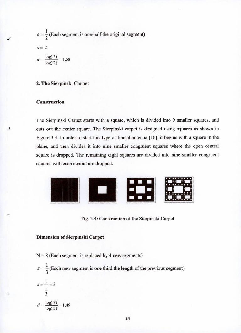
2. The Sierpinski Carpet
Construction
The Sierpinski Carpet starts with a square, which is divided into 9 smaller squares, and
-j cuts out the center square. The Sierpinski carpet is designed using squares as shown in
Figure 3.4. In order to start this type of fractal antenna [16], it begins with a square in the
plane, and then divides it into nine smaller congruent squares where the open central
square is dropped. The remaining eight squares are divided into nine smaller congruent
squares with each central are dropped.
........i
...
Fig. 3.4: Construction of the Sierpinski Carpet
Dimension of Sierpinski Carpet
N = 8 (Each segment is replaced by 4 new segments)
= -(Each new segment is one third the length of the previous segment)
d = Iog( 8) = 1.89
log( 3)
24
CHAPTER 4
Design of the Square Koch Fractal Antenna
4.1 Introduction
The Simplest example of antenna using fractal geometry is given by the Swedish
mathematician H. von Koch in 1904, which is known as Koch fractal. In this project a
wire square Koch fractal antenna is designed based on the first and second iterations of
square Koch curve geometry [23]. It is a very elementary example of fractal, as it follows
a simple rule of construction.
The square Koch curve [21] clearly shows the self-similarity of fractal. The same pattern
appears everywhere along the curve in different scale, from visible to infinitesimal.
The square Koch curve also shows the space filling property that means an infinite long
curve in a finite area and this property helps to make miniaturize[20] antennas.
4.2 Antenna Geometry
Figure 3.1 shows the first three iterations in the construction of the square Koch curve
[19]. This curve is simply constructed using iterative procedure beginning with the
initiator of the set as the unit line segment (iteration 0). The unit line segment is divided
into three segments, and the middle segment is removed. The middle segment is then
replaced with three equal segments, which are of the same length as the first segment,
which form a square (iteration 1). This step is the generator of the curve. At the next step
(iteration 2), the middle segment is removed from each of the five segments and each is
replaced with three equal segments as before. This process is repeated an infinite number
of times to produce square Koch curve [section-3 .7.1].
25
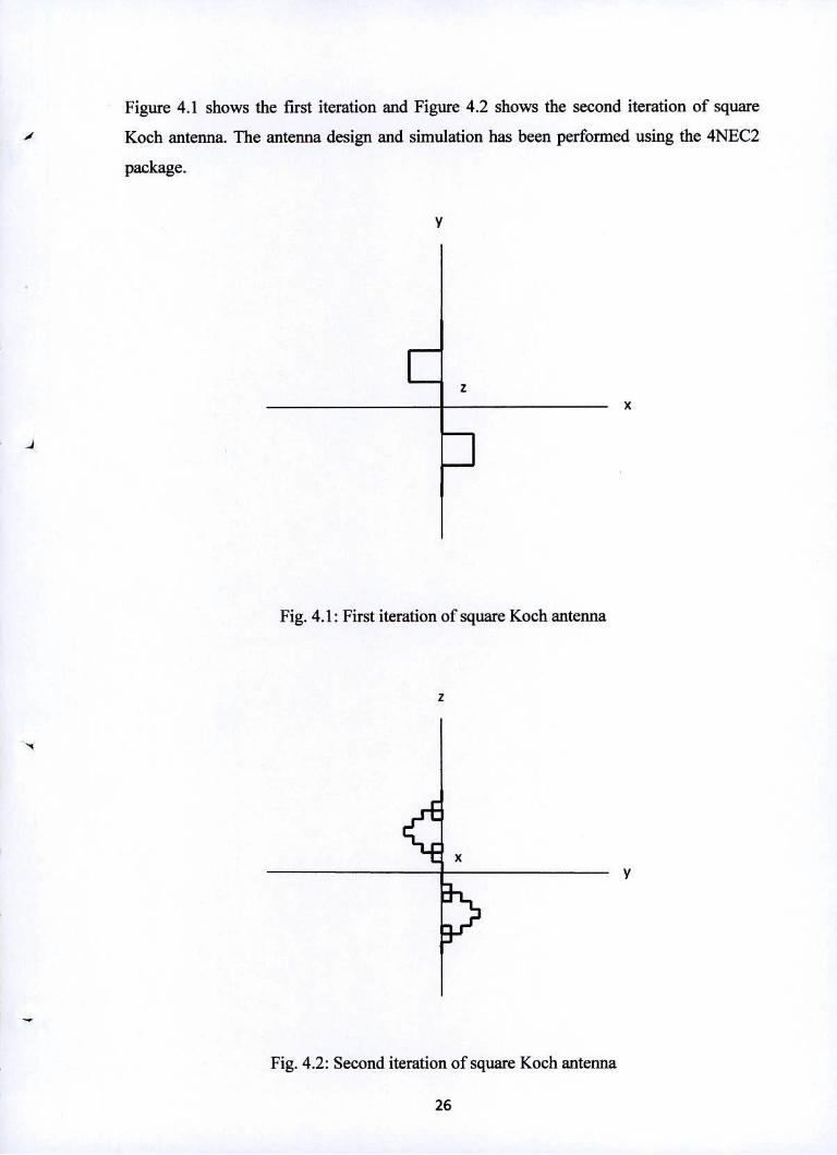
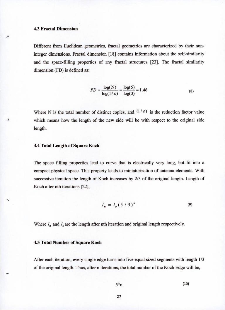
Figure 4.1 shows the first iteration and Figure 4.2 shows the second iteration of square
Af Koch antenna. The antenna design and simulation has been performed using the 4NEC2
package.
VA
-a
x
Fig. 4.1: First iteration of square Koch antenna
Fig. 4.2: Second iteration of square Koch antenna
26
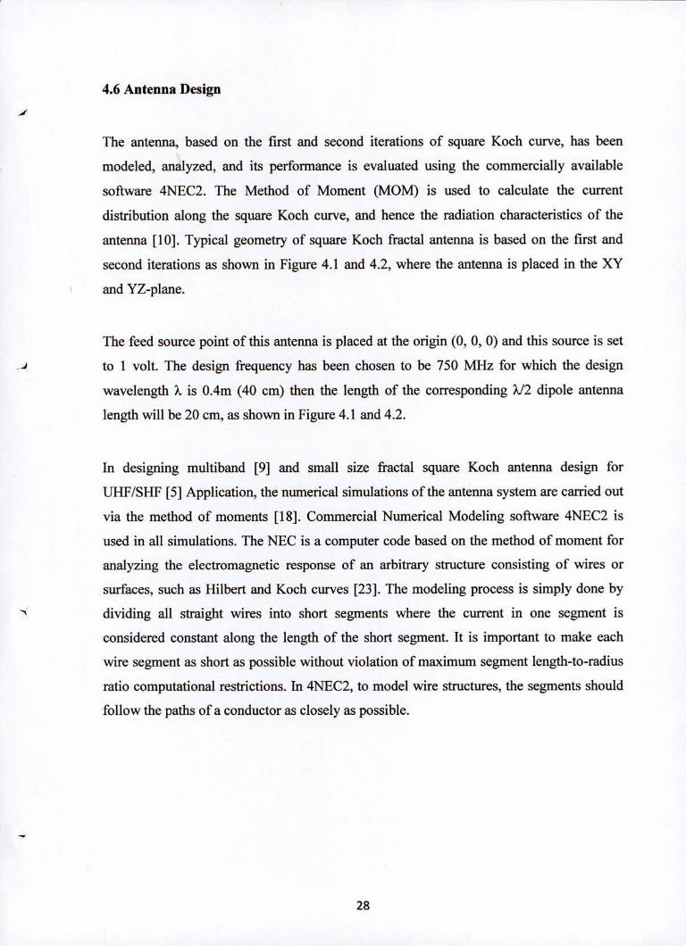
4.3 Fractal Dimension
Different from Euclidean geometries, fractal geometries are characterized by their non-
integer dimensions. Fractal dimension [18] contains information about the self-similarity
and the space-filling properties of any fractal structures [23]. The fractal similarity
dimension (FD) is defined as:
FD= log(N) Iog(5) 146
(8) log(1/s) Iog(3)
Where N is the total number of distinct copies, and 0 / ) is the reduction factor value
which means how the length of the new side will be with respect to the original side
length.
4.4 Total Length of Square Koch
The space filling properties lead to curve that is electrically very long, but fit into a
compact physical space. This property leads to miniaturization of antenna elements. With
successive iteration the length of Koch increases by 2/3 of the original length. Length of
Koch after nth iterations [22],
= 1(5 / 3) fl (9)
Where 1, and l are the length after nth iteration and original length respectively.
4.5 Total Number of Square Koch
After each iteration, every single edge turns into five equal sized segments with length 1/3
of the original length. Thus, after n iterations, the total number of the Koch Edge will be,
5A (10)
27
4.6 Antenna Design
A
The antenna, based on the first and second iterations of square Koch curve, has been
modeled, analyzed, and its perfonnance is evaluated using the commercially available
software 4NEC2. The Method of Moment (MOM) is used to calculate the current
distribution along the square Koch curve, and hence the radiation characteristics of the
antenna [10]. Typical geometry of square Koch fractal antenna is based on the first and
second iterations as shown in Figure 4.1 and 4.2, where the antenna is placed in the XY
and YZ-plane.
The feed source point of this antenna is placed at the origin (0, 0, 0) and this source is set
-J to 1 volt. The design frequency has been chosen to be 750 MHz for which the design
wavelength ?. is 0.4m (40 cm) then the length of the corresponding ?J2 dipole antenna
length will be 20 cm, as shown in Figure 4.1 and 4.2.
In designing multiband [9] and small size fractal square Koch antenna design for
UHF/SHF [5] Application, the numerical simulations of the antenna system are carried out
via the method of moments [18]. Commercial Numerical Modeling software 4NEC2 is
used in all simulations. The NEC is a computer code based on the method of moment for
analyzing the electromagnetic response of an arbitrary structure consisting of wires or
surfaces, such as Hilbert and Koch curves [23]. The modeling process is simply done by
dividing all straight wires into short segments where the current in one segment is
considered constant along the length of the short segment. It is important to make each
wire segment as short as possible without violation of maximum segment length-to-radius
ratio computational restrictions. In 4NEC2, to model wire structures, the segments should
follow the paths of a conductor as closely as possible.
28
CHAPTER 5
Simulation of Square Koch Fractal Antenna
5.1 Introduction
This chapter represents the simulation of multiband square Koch fractal antenna, where it
is shown that as the iterations are increased the bands of frequencies also increase and the
size is also reduced. The designed antenna has operating frequencies for first iteration are
of 496 MHz and 1430 MHz, and for second iteration are of 460 MHz, 1248 MHz, 1926
MHz and 4390 MHz with acceptable bandwidth, which has useful applications in
UHF/SHF. The radiation characteristics, SWR, return loss, input impedance, and gain of
the proposed antenna are described with 4NEC2 software package. Here, the antenna is
placed in the XY-plane for first iteration and in YZ-plane for second iteration.
Figure 3.1 shows the first three iterations in the construction of the square Koch curve
[19]. This curve is constructed using iterative procedure beginning with the initiator as the
unit line segment (iteration 0). The unit line segment is divided into three segments, and
the middle segment is removed. The middle segment is then replaced with three equal
segments, which are of the same length as the first segment, which form a square (iteration
1). At the next step (iteration 2), the middle segment is removed from each of the five
segments and each is replaced with three equal segments as before. This process is
repeated an infinite number of times to produce square Koch curve [section-3 .9.1].
5.2 Simulation Results
In this work, Method of Moment simulation code (NEC) is used to perform a detailed
study of SWR, reflection coefficient, input impedance, gain and radiation pattern
characteristics of the square Koch antenna in a free space.
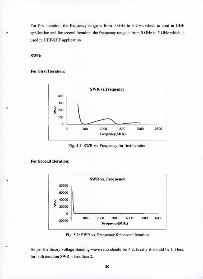
For first iteration, the frequency range is from 0 GHz to 3 GHz which is used in UHF
application and for second iteration, the frequency range is from 0 GHz to 5 GHz which is
used in UHF/SHF application.
SWR:
For First Iteration:
SWR vs.Frequency
400
300
PE 200
(I)
100
0
0 500 1000 1500 2000 2500
Frequency(MHz)
Fig. 5.1: SWR vs. Frequency for first iteration
For Second Iteration:
SWR vs. Frequency
80000
60000
40000
rIi 20000
0
w -20000 1000 2000 3000 4000 5000 6000
Frequency(MHz)
Fig. 5.2: SWR vs. Frequency for second iteration
As per the theory voltage standing wave ratio should be S 2. Ideally it should be 1. Here,
for both iteration SWR is less than 2.
30
iii.
Frequency(MHz)
10 r,)
j o -10
-20
-30
-40
1
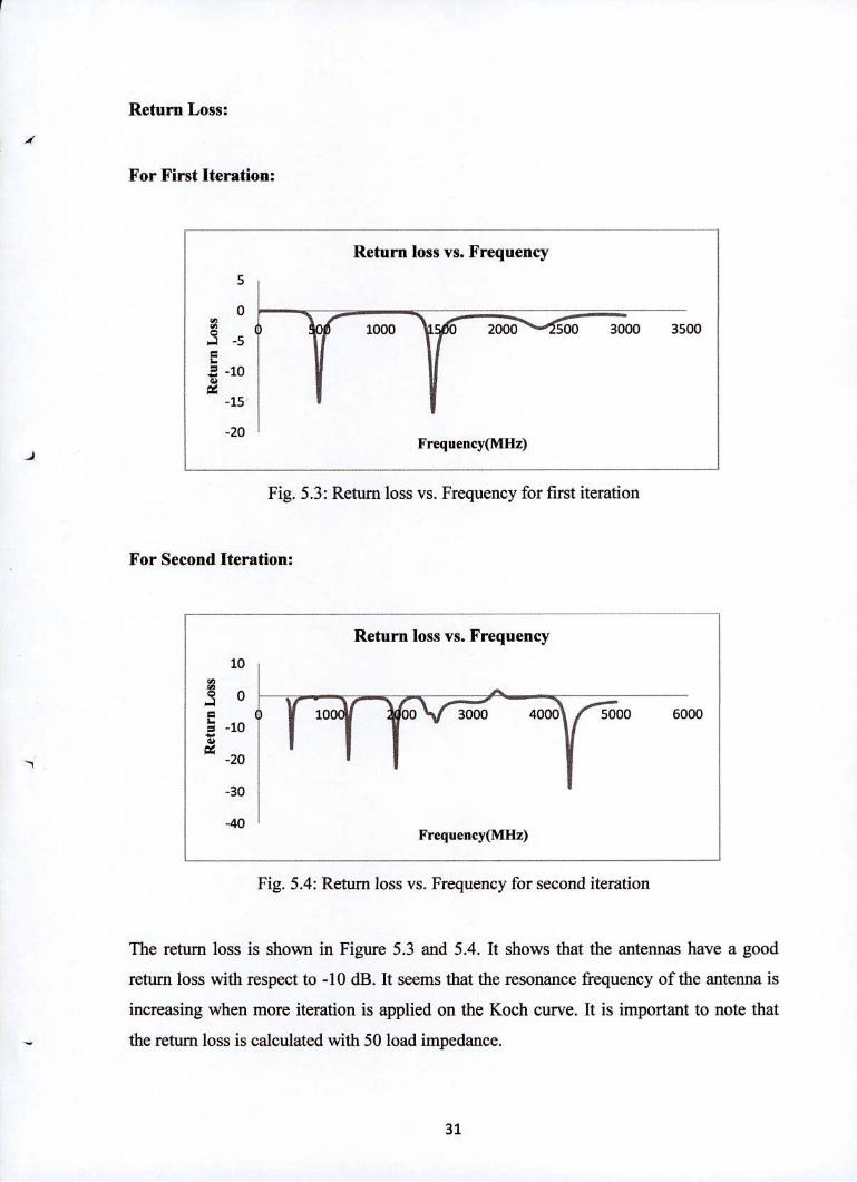
Return Loss:
For First Iteration:
Return loss vs. Frequency
(i000 - \dr 2000 500 3000 3500
-15
-20 Frequency(MHz)
Fig. 5.3: Return loss vs. Frequency for first iteration
For Second Iteration:
Return loss vs. Frequency
A
Fig. 5.4: Return loss vs. Frequency for second iteration
The return loss is shown in Figure 5.3 and 5.4. It shows that the antennas have a good
return loss with respect to -10 dB. It seems that the resonance frequency of the antenna is
increasing when more iteration is applied on the Koch curve. It is important to note that
the return loss is calculated with 50 load impedance.
31
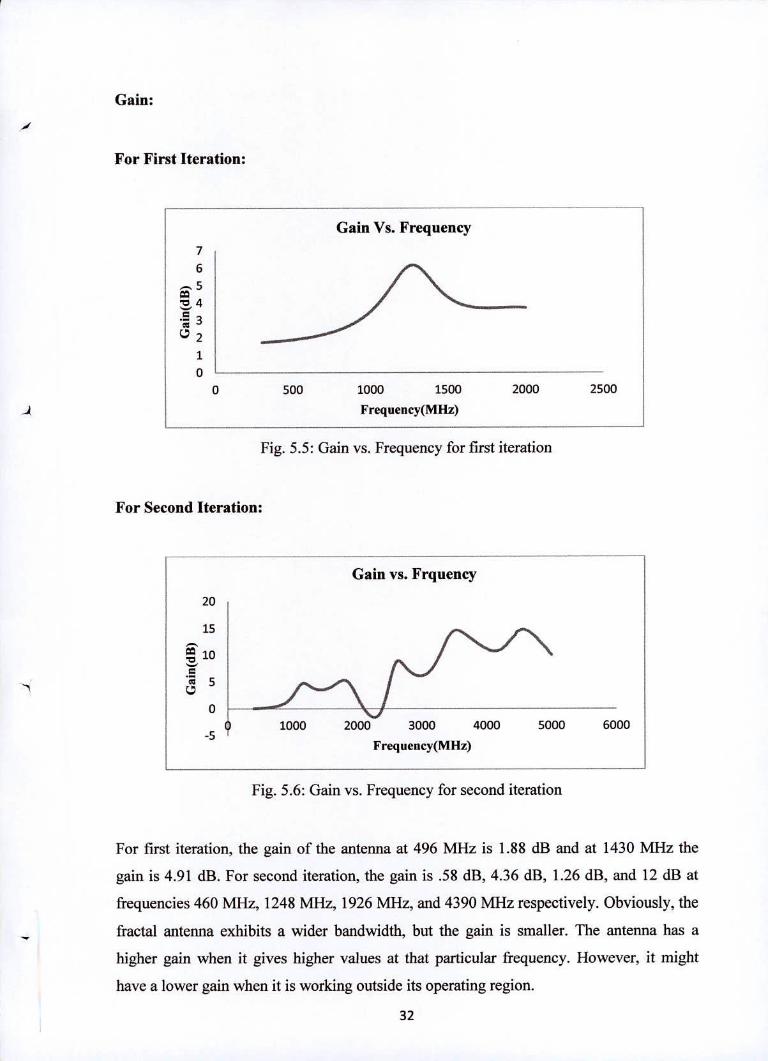
Gain:
A
For First Iteration:
Gain Vs. Frequency
0 500 1000 1500 2000 2500
Frequency(MHz)
Fig. 5.5: Gain vs. Frequency for first iteration
For Second Iteration:
Gain vs. Frquency
20
15
10
0
-5 I,
Frequency(MHz)
Fig. 5.6: Gain vs. Frequency for second iteration
For first iteration, the gain of the antenna at 496 MHz is 1.88 dB and at 1430 MHz the
gain is 4.91 dB. For second iteration, the gain is .58 dB, 4.36 dB, 1.26 dB, and 12 dB at
frequencies 460 MHz, 1248 MHz, 1926 MHz, and 4390 MHz respectively. Obviously, the
fractal antenna exhibits a wider bandwidth, but the gain is smaller. The antenna has a
higher gain when it gives higher values at that particular frequency. However, it might
have a lower gain when it is working outside its operating region.
32
ECEI
Frequency(MHz)
5000
CZ 4000
3000
2000
•.:: 1000 = 0
-1000
'1
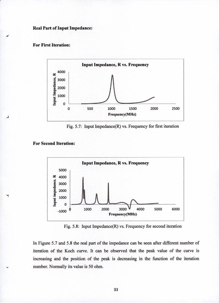
Real Part of Input Impedance:
For First Iteration:
Input Impedance, R vs. Frequency
4000
1
2000 CL
1000
=
0 500 1000 1500 2000 2500
J Frequency(MHz)
Fig. 5.7: Input Impedance(R) vs. Frequency for first iteration
For Second Iteration:
Input Impedance, R vs. Frequency
Fig. 5.8: Input Impedance(R) vs. Frequency for second iteration
In Figure 5.7 and 5.8 the real part of the impedance can be seen after different number of
iteration of the Koch curve. It can be observed that the peak value of the curve is
increasing and the position of the peak is decreasing in the function of the iteration
number. Normally its value is 50 ohm.
33
'I'll"]
1000
0
-1000
-2000
I,IIIi1 -J Frequency(MHz)
Frequency(MHz)
3000
< 2000
1000
E -1000
-2000
-3000
I
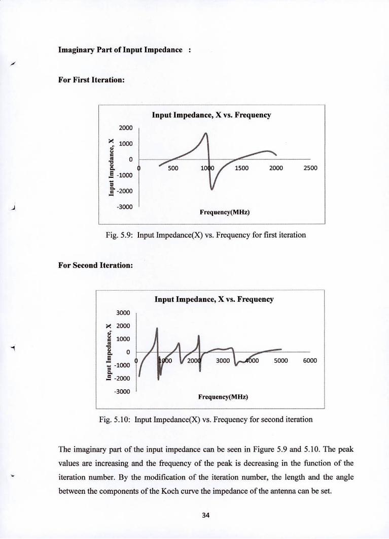
Imaginary Part of Input Impedance
For First Iteration:
Input Impedance, X vs. Frequency
Fig. 5.9: Input Impedance(X) vs. Frequency for first iteration
For Second Iteration:
Input Impedance, X vs. Frequency
Fig. 5.10: Input Impedance(X) vs. Frequency for second iteration
The imaginary part of the input impedance can be seen in Figure 5.9 and 5.10. The peak
values are increasing and the frequency of the peak is decreasing in the function of the
iteration number. By the modification of the iteration number, the length and the angle
between the components of the Koch curve the impedance of the antenna can be set.
34
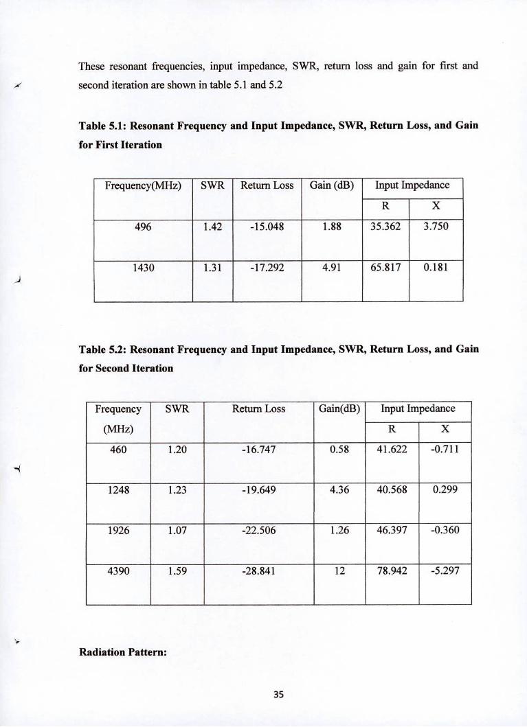
These resonant frequencies, input impedance, SWR, return loss and gain for first and
.41 second iteration are shown in table 5.1 and 5.2
Table 5.1: Resonant Frequency and Input Impedance, SWR, Return Loss, and Gain
for First Iteration
Frequency(MHz) SWR Return Loss Gain (dB) Input Impedance
R X
496 1.42 -15.048 1.88 35.362 3.750
1430 1.31 -17.292 4.91 65.817 0.181
Table 5.2: Resonant Frequency and Input Impedance, SWR, Return Loss, and Gain
for Second Iteration
Frequency
(MHz)
SWR Return Loss Gain(dB) Input Impedance
R X
460 1.20 -16.747 0.58 41.622 -0.711
1248 1.23 -19.649 4.36 40.568 0.299
1926 1.07 -22.506 1.26 46.397 -0.360
4390 1.59 -28.841 12 78.942 -5.297
Radiation Pattern:
35
J
F
'I
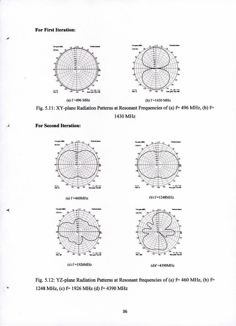
For First Iteration:
1:. T.l.q 11 r YSeCS ila I
42
75
rT
•-.s..:3
7"
21, ...: .
p_ 91
IS Im u is .1 PS. IkS 114 is i
(a) f =496 MHz (b) f1430 MHz
Fig. 5.11: XY-plane Radiation Patterns at Resonant Frequencies of (a) f= 496 MHz, (b) f=
1430 MHz
For Second Iteration:
T.i9.4 0Z
11418*
has
IW
165 065
(a) f =460MHz
Y..14d ii...
lt%MN.
14
TTT'
0360 PS- 80 60 ISO
165
(C) f =1926MHz
02
75
US
165
(d)f =4390MHz
Fig. 5.12: YZ-plane Radiation Patterns at Resonant frequencies of(a) f 460 MHz, (b) f 3.. 1248 MHz, (c) f= 1926 MHz (d) f 4390 MHz
36
The analysis for radiation patterns for Fractal Koch antennas for the first and second
/ iterations is discussed in Fig. 5.11 and 5.12. The radiation pattern for the 1st iteration at
496 MHz and 1430 MHz is depicted in Figure 5.11 and the radiation patterns for second
iteration at 460 MHz, 1248 MHz, 1926 MHz and 4390 MHz are shown in Figure 5.12.
The measured radiation patterns show that the antennas are linearly polarized.
The simulation results show that this antenna can be efficiently operated as a multiband
antenna. The proposed antenna has two resonance bands for first iteration at frequencies of
496 MHz and 1430 MHz. Also the antenna has four resonance bands for second iteration
at frequencies 460 MHz, 1248 MHz, 1926 MHz and 4390 MHz. From this, we can say
that, as the iterations are increased, the band of frequencies also increase. At these
frequencies the antenna has SWR<2, Return loss is less than -10. The gains at these
frequencies are also acceptable.
5.3 Miniaturization Technique of Square Koch Fractal Antenna
With successive iteration the length of Koch increases by 2/3 of the original length.
Length of Koch after nth iterations,
l = 1(5 /3 (Ii)
Where l and 1 are the length after nth iteration and original length respectively. And,
after nth iterations, the total number of the Koch Edge will be
5An (12)
By using the above two formulas, the miniaturization of square Koch fractal can be
calculated.
37
CHAPTER 6
/
Conclusion
6.1 Conclusion
In this project, the square Koch fractal antenna based on the first and second iterations is
investigated and its performance is evaluated. The simulation results show that this
antenna can be efficiently operated as a multiband antenna and it is also compact in size.
The proposed antenna has two resonance bands for first iteration at frequencies of 496
MHz and 1430 MHz. Also the antenna has four resonance bands for second iteration at
frequencies 460 MHz, 1248 MHz, 1926 MHz, and 4390 MHz. From this, we can say that,
as the iterations are increased, the band of frequencies also increase but the physical length
does not increase. At these frequencies the antenna has SWR<2, Return loss is less than -
10. The gains at these frequencies are also acceptable. The radiation pattern is very
uniform in all directions. And the antenna has the required band for UHF/SHF. So, this
antenna can operate as a small multiband antenna in the TJHF/SHF applications.
38

REFERENCES
B.B. Mandeibrot, "The Fractal geometry of Nature," New York, 1983.
Balanis C.A., "Antenna Theory: Analysis and Design", Second Edition, New
York, John Wiley& Sons, Inc., 2003.
K.D Prasad, "Antennas & wave propagation", ISBN no. 81-7634-025-4, third
edition.
Jibrael, F. J.: Miniature Dipole Antenna Based on the Fractal Square Koch Curve,
European Journal of Scientific Research, Vol. 21, No.4, 2008, pp. 700-706.
Zainud-Deen, S. H., Malirat, H. A., Awadalla, K. H.: Fractal Antenna for Passive
UHF RFID Applications, Progress In Electromagnetic Research B, Vol. 16, 2009,
pp. 209-228.
Mirzapour, B. and H. R. Hassani, Size reduction and bandwidth enhancement of
snowflake fractal antenna," Microwaves, Antennas &Propagation, lET, 180-187,
Mar. 2008.
D. H. Werner and S. Ganguly, "An Overview of Fractal Antennas Engineering
Research", IEEE Antennas and Propagation Magazine, vol. 45, no. 1, pp. 38-57,
February 2003.
T. Tiehong and Z. Zheng, " A Novel Multiband Antenna: Fractal Antenna",
Electronic letter, Proceedings of ICCT —2003, pp: 1907-1910.
Lee. Y., Yeo. J., Mittra R., Ganguly S. and Tenbarge J., "Fractal and Multiband
Communication Antennas", IEEE Conf. on Wireless Communication Technology,
pp. 273-274, 2003. fr
39
Cohen N., "Fractal Antennas: Part I", Communications Quarterly, summer, pp. 7-
1 22, 1995.
Cohen N., "Fractal Antennas: Part 2", Communications Quarterly, summer, pp. 53-
66, 1996.
Kravchenko V.F., "The theory of fractal antenna arrays", Antenna Theory and
Techniques IVth Inter. Conf., Vol. 1, pp. 183- 189, 2003.
Gianvittorio, J., Fractal antenna: Design, characterization, and Progress In
Electromagnetics Research, PIER 100, 2010.
) Nima Bayatmaku, Parisa Lotfi, Mohammadnaghi Azarmanesh, Member, IEEE,
and Saber Soltani," Design of Simple Multiband Patch Antenna For Mobile
Communication Applications Using New E-Shape Fractal", IEEE antennas and
wireless propagation letters, vol. 10, 2011.
Gianviffwb J.P. and Rahmat-Samii Y., "Fractals Antennas: A novel Antenna
Miniaturization Technique, and Applications", IEEE Antennas and Propagation
Magazine, Vol. 44, pp. 20- 36, 2002.
A 16. Kuem C. Hwang, "A Modified Sierpinski Fractal Antenna for Multiband
Application" proceedings of the IEEE Antennas and Propagation Letters, Vol.
6, 2007.
Yeo J. and Mittra R., "Modified Sierpinski Gasket Patch Antenna for Multiband
Applications", IEEE International Symp. On Antennas and Propagation Digest,
2001.
K.J. Vinoy, K.A. Jose, and V.K. Varadan, "Multiband characteristics and fractal
dimension of dipole antennas with Koch curve geometry," IEEE 2002 AP-S Inter.
Symp., 2002.
40
Puente C., Romeu J., Pous R., Ramias J. and Hijazo A., "Small but long Koch
fractal monopole", lEE Electronic Letters, Vol. 34, 1, pp. 9-10, 1998.
C.P. Baliarda, J. Romeu, and A. Cardama, "The Koch monopole: A small fractal
antenna," IEEE Trans. Ant. Propagat., vol. 48 pp. 1773-1781, 2000.
S.H Zainud-Deen, K.H. Awadalla S.A. Khamis and N.d. El-shalaby, March 16-18,
2004. Radiation and Scattering from Koch Fractal Antennas. 21st National Radio
Science Conference (NRSC), B8 - 1-9.
JAMIL, A., YUSOFF, M.Z., YAHYA, N. Small Koch fractal antennas for wireless
local area network. In Proceedings of the International Conference on
Communication Systems ICCS 2010. Singapore: National University of Singapore,
2010, p. 104-108.
BEST, S.R. On the resonant properties of the Koch fractal and other wire
monopole antennas. IEEE Antennas and Wireless Propagation Letter, 2002, vol. 1,
no. 1, p. 74-76.
JAMIL, A., YUSOFF, M.Z., YAHYA, N. Small Koch fractal antennas for wireless
local area network. In Proceedings of the International Conference on
Communication Systems ICCS 2010. Singapore: National University of Singapore,
2010, p. 104-108.
www. fractus. com, 2000.
www. fractenna. corn, 2000.
01
41
![A RECONFIGURABLE U-KOCH MICROSTRIP ANTENNA FOR … · geometries, and that Koch fractal antennas are multiband structures. The authors of [10] related multiple resonant frequencies](https://img.pdfslide.us/doc/110x75/5e764ec1b5799e0f2317c4ff/a-reconfigurable-u-koch-microstrip-antenna-for-geometries-and-that-koch-fractal.jpg)


![Multiband Monopole Antenna with Sector-Nested Fractalfractal antennas in recent years include Sierpinski fractal antenna[8], Koch fractal antenna [9] and Minkowski antenna [10] . In](https://img.pdfslide.us/doc/110x75/5e76c468024e970eb01c097c/multiband-monopole-antenna-with-sector-nested-fractal-fractal-antennas-in-recent.jpg)
![FRACTAL KOCH MULTIBAND TEXTILE ANTENNA … · Koch fractal antenna is able to reduce size up to 7% for flrst iteration and up to 26% for series iteration [19]. Koch fractal-slotted](https://img.pdfslide.us/doc/110x75/5fb1830efc40811fac69fceb/fractal-koch-multiband-textile-antenna-koch-fractal-antenna-is-able-to-reduce-size.jpg)