Embed Size (px)
Citation preview

MULTIAGENT MOVING TARGET SEARCH
IN FULLY VISIBLE GRID ENVIRONMENTS WITH NO SPEED DIFFERENCE
CAN EROGUL
DECEMBER 2006
MULTIAGENT MOVING TARGET SEARCH
IN FULLY VISIBLE GRID ENVIRONMENTS WITH NO SPEED DIFFERENCE
A THESIS SUBMITTED TO
THE GRADUATE SCHOOL OF NATURAL AND APPLIED SCIENCES
OF
MIDDLE EAST TECHNICAL UNIVERSITY
BY
CAN EROGUL
IN PARTIAL FULFILLMENT OF THE REQUIREMENTS
FOR
THE DEGREE OF MASTER OF SCIENCE
IN
COMPUTER ENGINEERING
DECEMBER 2006

Approval of the Graduate School of Natural and Applied Sciences
Prof. Dr. Canan OZGEN
Director
I certify that this thesis satisfies all the requirements as a thesis for the degree of
Master of Science.
Prof. Dr. Ayse KIPER
Head of Department
This is to certify that we have read this thesis and that in our opinion it is fully
adequate, in scope and quality, as a thesis for the degree of Master Of Science.
Prof. Dr. Faruk POLAT
Supervisor
Examining Committee Members
Assoc. Prof. Dr. Gokturk UCOLUK (METU,CENG)
Prof. Dr. Faruk POLAT (METU,CENG)
Assoc. Prof. Dr. Ismail Hakkı TOROSLU (METU,CENG)
Asist. Prof. Dr. Afsar SARANLI (METU,EE)
Dr. Onur Tolga SEHITOGLU (METU,CENG)

I hereby declare that all information in this document has been obtained and pre-
sented in accordance with academic rules and ethical conduct. I also declare that,
as required by these rules and conduct, I have fully cited and referenced all material
and results that are not original to this work.
Name, Lastname : Can Erogul
Signature :
iii
Abstract
MULTIAGENT MOVING TARGET SEARCH
IN FULLY VISIBLE GRID ENVIRONMENTS WITH NO SPEED
DIFFERENCE
Erogul, Can
M.Sc., Department of Computer Engineering
Supervisor: Prof. Dr. Faruk Polat
December 2006, 59 pages
In this thesis, a new real-time multi-agent moving target pursuit algorithm and
a moving target algorithm are developed and implemented. The environment is a
grid world, in which a coordinated team of agents cooperatively blocks the possible
escape routes of an intelligent target in real-time.
Most of the moving target search algorithms presume that the agents are faster
than the targets, so the pursuit is sure to end in favor of the agents. In this work, we
relax this assumption and assume that all the moving objects have the same speed.
This means that the agents must find a new approach for success in the pursuit,
other than just chasing the targets. When the search agents and the moving targets
are moving with the same speed, we need more than one search agent which can
coordinate with the other agents to capture the target.
Agents are allowed to communicate with each other.
We propose a multi-agent search algorithm for this problem. To our best knowl-
edge, there is no alternative algorithm designed based on these assumptions. The
proposed algorithm is compared to the modified versions of its counterparts (A*,
MTS and its derivatives) experimentally.
iv

Keywords: Multi-Agent Moving Target Search, Moving Target Search, Real-Time
Search.
v
Oz
TAMAMI GORULEN GRID ORTAMDA COKLU-AJANLA AYNI
HIZDAKI HAREKETLI HEDEF TAKIBI
Erogul, Can
Yuksek Lisans, Bilgisayar Muhendisligi Bolumu
Tez Yoneticisi: Prof. Dr. Faruk Polat
Aralık 2006, 59 sayfa
Bu calısmada, yeni bir coklu ajan hareketli hedef kovalama algoritması ve hareketli
hedef algoritması gelistirilecektir. Ortam olarak grid dunyası kullanılacak, bu ortam-
daki koordineli ajan takımı hareketli hedefin olası kacıs guzergahlarını kapatmak icin
gercek zamanda plan yapacaktır.
Cogu hareketli hedef arama algoritması ajanların hedeflerden daha hızlı oldugunu
varsayar, bu da takibin ajanların lehine sonlanmasına yol acar. Bu calısmadaki ana
amacımız, bu varsayımı hafifletmektir. Hedeflerin de ajanların da aynı hızda gittigini
varsayarsak, ajanların hedeflerini yakalamak icin hedefleri kovalamaktan baska yeni
bir yaklasım bulmaları gerekir. Bu kosullarda kovalama isini esgudum icinde yuruten
birden fazla ajana ihtiyac dogar.
Ajanlar arasında iletisim serbesttir.
Bu problem icin bir coklu ajan arama algoritması oneriyoruz. Bildigimiz kadarıyla
bu varsayımlara dayanarak tasarlanmıs baska bir algoritma bulunmamaktadır. O-
nerilen algoritma, ona karsı gelen diger algoritmaların turevleri ile (A*, MTS ve
turevleri) deneysel olarak karsılastırılacaktır.
vi

Anahtar Kelimeler: Coklu-Ajan Hareketli Hedef Takibi, Hareketli Hedef Arama,
Gercek Zamanlı Arama.
vii

To my family.
viii

Acknowledgments
I would like to thank my supervisor Prof. Dr. Faruk Polat for his patience and
guidance during the development of my thesis.
I would like to thank my brother Umut Erogul, for his ideas and support.
I would like to also thank Cagatay Undeger for his help and ideas.
Finally, I would like to thank my parents and my aunt Dicle Erogul for their under-
standing and support.
ix
Table of Contents
Plagiarism . . . . . . . . . . . . . . . . . . . . . . . . . . . . . . . . . . . . . . . . . . . . . . . . . . . . . . . . . . . . iii
Abstract . . . . . . . . . . . . . . . . . . . . . . . . . . . . . . . . . . . . . . . . . . . . . . . . . . . . . . . . . . . . . . iv
Oz . . . . . . . . . . . . . . . . . . . . . . . . . . . . . . . . . . . . . . . . . . . . . . . . . . . . . . . . . . . . . . . . . . . . . . vi
Acknowledgments . . . . . . . . . . . . . . . . . . . . . . . . . . . . . . . . . . . . . . . . . . . . . . . . . . . ix
Table of Contents . . . . . . . . . . . . . . . . . . . . . . . . . . . . . . . . . . . . . . . . . . . . . . . . . . . x
List of Tables . . . . . . . . . . . . . . . . . . . . . . . . . . . . . . . . . . . . . . . . . . . . . . . . . . . . . . . . xii
List of Figures . . . . . . . . . . . . . . . . . . . . . . . . . . . . . . . . . . . . . . . . . . . . . . . . . . . . . . . xiv
List of Algorithms . . . . . . . . . . . . . . . . . . . . . . . . . . . . . . . . . . . . . . . . . . . . . . . . . . xv
CHAPTER
1 Introduction . . . . . . . . . . . . . . . . . . . . . . . . . . . . . . . . . . . . . . . . . . . . . . . . . . . . . . 1
1.1 Motivations . . . . . . . . . . . . . . . . . . . . . . . . . . . . . . . . . 1
1.2 Goals of this Study . . . . . . . . . . . . . . . . . . . . . . . . . . . . . 2
1.3 Outline of the Thesis . . . . . . . . . . . . . . . . . . . . . . . . . . . . 3
2 Related Work . . . . . . . . . . . . . . . . . . . . . . . . . . . . . . . . . . . . . . . . . . . . . . . . . . . . 5
2.1 A* . . . . . . . . . . . . . . . . . . . . . . . . . . . . . . . . . . . . . . 6
2.2 Real-Time A* . . . . . . . . . . . . . . . . . . . . . . . . . . . . . . . . 7
x
2.3 Learning Real-Time A* . . . . . . . . . . . . . . . . . . . . . . . . . . 9
2.4 Dynamic A* . . . . . . . . . . . . . . . . . . . . . . . . . . . . . . . . . 9
2.5 Moving Target Search . . . . . . . . . . . . . . . . . . . . . . . . . . . 12
2.6 Multi-Agent Real-Time A* . . . . . . . . . . . . . . . . . . . . . . . . 13
2.7 Multi-Agent Moving Target Search . . . . . . . . . . . . . . . . . . . . 14
3 Multi-Agent Moving Target Pursuit . . . . . . . . . . . . . . . . . . . . . . . . . . 16
3.1 Problem Description . . . . . . . . . . . . . . . . . . . . . . . . . . . . 16
3.2 Agent Design . . . . . . . . . . . . . . . . . . . . . . . . . . . . . . . . 17
3.2.1 Moving Target Algorithm . . . . . . . . . . . . . . . . . . . . . 17
3.2.2 Coordinated Agent Algorithm . . . . . . . . . . . . . . . . . . . 20
4 Experimental Results . . . . . . . . . . . . . . . . . . . . . . . . . . . . . . . . . . . . . . . . . . . . 24
4.1 Test Environment . . . . . . . . . . . . . . . . . . . . . . . . . . . . . . 24
4.2 Test Results . . . . . . . . . . . . . . . . . . . . . . . . . . . . . . . . . 26
5 Conclusion and Future Work . . . . . . . . . . . . . . . . . . . . . . . . . . . . . . . . . . 54
5.1 Conclusion . . . . . . . . . . . . . . . . . . . . . . . . . . . . . . . . . 54
5.2 Future Work . . . . . . . . . . . . . . . . . . . . . . . . . . . . . . . . 55
5.2.1 Future Work on The Environment Properties . . . . . . . . . . 55
5.2.2 Future Work on The Target Algorithm . . . . . . . . . . . . . . 55
5.2.3 Future Work on The Agent Algorithm . . . . . . . . . . . . . . 56
References . . . . . . . . . . . . . . . . . . . . . . . . . . . . . . . . . . . . . . . . . . . . . . . . . . . . . . . . . . . . 58
xi
List of Tables
4.1 Hand-Crafted Map Test Results . . . . . . . . . . . . . . . . . . . . . . 33
4.2 Test Results Of Generated Maps with Smaller Obstacles (x:10, y:10
Obstacle:10%) . . . . . . . . . . . . . . . . . . . . . . . . . . . . . . . . 36
4.3 Test Results Of Generated Maps with Smaller Obstacles (x:10, y:10
Obstacle:20%) . . . . . . . . . . . . . . . . . . . . . . . . . . . . . . . . 37
4.4 Test Results Of Generated Maps with Smaller Obstacles (x:10, y:10
Obstacle:30%) . . . . . . . . . . . . . . . . . . . . . . . . . . . . . . . . 38
4.5 Test Results Of Generated Maps with Smaller Obstacles (x:20, y:20
Obstacle:10%) . . . . . . . . . . . . . . . . . . . . . . . . . . . . . . . . 39
4.6 Test Results Of Generated Maps with Smaller Obstacles (x:20, y:20
Obstacle:20%) . . . . . . . . . . . . . . . . . . . . . . . . . . . . . . . . 40
4.7 Test Results Of Generated Maps with Smaller Obstacles (x:20, y:20
Obstacle:30%) . . . . . . . . . . . . . . . . . . . . . . . . . . . . . . . . 41
4.8 Test Results Of Generated Maps with Smaller Obstacles (x:30, y:30
Obstacle:10%) . . . . . . . . . . . . . . . . . . . . . . . . . . . . . . . . 42
4.9 Test Results Of Generated Maps with Smaller Obstacles (x:30, y:30
Obstacle:20%) . . . . . . . . . . . . . . . . . . . . . . . . . . . . . . . . 43
4.10 Test Results Of Generated Maps with Smaller Obstacles (x:30, y:30
Obstacle:30%) . . . . . . . . . . . . . . . . . . . . . . . . . . . . . . . . 44
4.11 Test Results Of Generated Maps with Bigger Obstacles (x:10, y:10
Obstacle:10%) . . . . . . . . . . . . . . . . . . . . . . . . . . . . . . . . 45
4.12 Test Results Of Generated Maps with Bigger Obstacles (x:10, y:10
Obstacle:20%) . . . . . . . . . . . . . . . . . . . . . . . . . . . . . . . . 46
4.13 Test Results Of Generated Maps with Bigger Obstacles (x:10, y:10
Obstacle:30%) . . . . . . . . . . . . . . . . . . . . . . . . . . . . . . . . 47
xii
4.14 Test Results Of Generated Maps with Bigger Obstacles (x:20, y:20
Obstacle:10%) . . . . . . . . . . . . . . . . . . . . . . . . . . . . . . . . 48
4.15 Test Results Of Generated Maps with Bigger Obstacles (x:20, y:20
Obstacle:20%) . . . . . . . . . . . . . . . . . . . . . . . . . . . . . . . . 49
4.16 Test Results Of Generated Maps with Bigger Obstacles (x:20, y:20
Obstacle:30%) . . . . . . . . . . . . . . . . . . . . . . . . . . . . . . . . 50
4.17 Test Results Of Generated Maps with Bigger Obstacles (x:30, y:30
Obstacle:10%) . . . . . . . . . . . . . . . . . . . . . . . . . . . . . . . . 51
4.18 Test Results Of Generated Maps with Bigger Obstacles (x:30, y:30
Obstacle:20%) . . . . . . . . . . . . . . . . . . . . . . . . . . . . . . . . 52
4.19 Test Results Of Generated Maps with Bigger Obstacles (x:30, y:30
Obstacle:30%) . . . . . . . . . . . . . . . . . . . . . . . . . . . . . . . . 53
xiii
List of Figures
1.1 Which path would you chose for H2? . . . . . . . . . . . . . . . . . . . 3
2.1 MAMTS: Belief sets (left) and filtered belief set (right) . . . . . . . . 15
3.1 The Mid-Point Explanation . . . . . . . . . . . . . . . . . . . . . . . . 21
3.2 MAMTP Example . . . . . . . . . . . . . . . . . . . . . . . . . . . . . 22
4.1 A Long Path . . . . . . . . . . . . . . . . . . . . . . . . . . . . . . . . 29
4.2 Success Ratio of the Algorithms over The Obstacle Ratio on 10 X 10
Maps with Smaller Obstacles . . . . . . . . . . . . . . . . . . . . . . . 30
4.3 Success Ratio of the Algorithms over The Obstacle Ratio on 20 X 20
Maps with Smaller Obstacles . . . . . . . . . . . . . . . . . . . . . . . 30
4.4 Success Ratio of the Algorithms over The Obstacle Ratio on 30 X 30
Maps with Smaller Obstacles . . . . . . . . . . . . . . . . . . . . . . . 31
4.5 Success Ratio of the Algorithms over The Obstacle Ratio on 10 X 10
Maps with Bigger Obstacles . . . . . . . . . . . . . . . . . . . . . . . . 31
4.6 Success Ratio of the Algorithms over The Obstacle Ratio on 20 X 20
Maps with Bigger Obstacles . . . . . . . . . . . . . . . . . . . . . . . . 32
4.7 Success Ratio of the Algorithms over The Obstacle Ratio on 30 X 30
Maps with Bigger Obstacles . . . . . . . . . . . . . . . . . . . . . . . . 32
xiv
List of Algorithms
1 A* . . . . . . . . . . . . . . . . . . . . . . . . . . . . . . . . . . . . . . 7
2 RTA* . . . . . . . . . . . . . . . . . . . . . . . . . . . . . . . . . . . . 8
3 LRTA* . . . . . . . . . . . . . . . . . . . . . . . . . . . . . . . . . . . 9
4 D* Lite Second Version . . . . . . . . . . . . . . . . . . . . . . . . . . 11
5 MTS . . . . . . . . . . . . . . . . . . . . . . . . . . . . . . . . . . . . 12
6 Moving Target Algorithm . . . . . . . . . . . . . . . . . . . . . . . . . 19
7 Multi-Agent Moving Target Pursuit Algorithm . . . . . . . . . . . . . 23
xv
Chapter 1
Introduction
1.1 Motivations
If you were a kid, playing a simple computer game (e.g. pacman variations), and
watching some agents chasing you, you wouldn’t be amazed by the artificial intelli-
gence or the coordination of the agents, because the non-cheating agents (which use
the current algorithms in literature) wouldn’t try to corner you, or cut your way, they
will simply chase you. Clearly, the games we play today are not that boring. The
games don’t need to be fair, they need to be fun, so if your way has to be cut by some
agent, then an agent is created on your way, or an existing agent gets teleported to
your possible future path. Generally the artificial intelligence in the computer games
cheats more, when the difficulty of the game is set to a higher level. We are interested
in non-cheating algorithms, which can get similar satisfying results.
The paths mentioned above are computed by the path planning algorithms. The
classic search algorithms, such as A*, RTA* and MTS, cannot get satisfying results
on the problem mentioned above. These algorithms compute paths between a start
node and a target node according to distance values, which can be determined by
search (expensive) or by heuristics (inaccurate). The agents may not have enough
time to make an optimal decision, they may have to decide on the next step in the
shortest possible time. The algorithms that determine the next move in such a short
time are called real-time search algorithms. A* algorithm computes the whole path
before making the first move, where real-time search algorithms such as Real-Time
A* plans its next move and executes it. Most path search algorithms are designed
for stationary targets, but in computer games and many other domains, the targets
may be moving.
1
Moving target search algorithms assume that the agents move faster than the
target, to guarantee the capture of the target. Without this assumption, the target
can evade capture. This is natural when there is only one agent. But if there were
multiple agents (even 2 is enough in 8 neighborhood grid domain) controlled by
humans, who have the full view of the grid map, no target would be able to elude the
capture, even if they had the same speed. Unfortunately the algorithms that exist
today are not capable enough to take advantage of multiple agents.
1.2 Goals of this Study
The aim of this thesis is to develop a multi-agent search algorithm, which takes advan-
tage of cooperation among the team members for intervening the possible alternative
paths of the moving target. We propose a coordinated hunter algorithm, in which an
agent computes the shortest path to the target, but if there is another agent closer
to the mid-point of that path, that agent can guard the path in question, therefore
our agent searches for other alternative paths.
The environment is assumed to be a planar grid, and all of the agents have full
vision of the grid and the coordinates of the other agents. Maps with different sizes
and obstacle ratios were randomly generated in addition to the hand-crafted maps, on
which more distinctive tests could be run for the cooperation of the agents. Agents
are initially located at the same corner of the map, and the target is positioned
randomly. The proposed algorithm is compared with A* and MTS derivatives.
The ultimate goal is to obtain shorter paths and shorter run times in the overall
simulation instead of shorter computation time per turn.
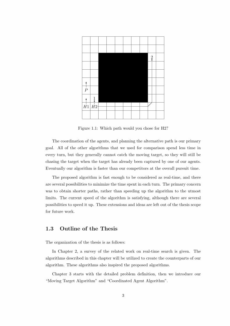
Consider the case given in Figure 1.1: Assume that all agents move at the same
speed, i.e., move concurrently. There are two agents H1 and H2, and a single target
P . Traditional path search algorithms such as A*, RTA* would propose to move
upward for both H1 and H2. However the best strategy for hunters is to move in
opposite directions around the obstacle to capture the target, instead of just chasing
the target. Any human would follow this simple strategy without hesitation. However
if the hunters are controlled with the algorithms in the literature, the second hunter
H2 follows the target just like its partner, chasing the target step by step, they will
continue to cycle around the obstacle forever. Even MAMTS algorithm, which is the
algorithm with the maximum cooperation currently in the literature, goes up to the
node 1.
2
P
6
H1 H26 6
1
¡¡
62
Figure 1.1: Which path would you chose for H2?
The coordination of the agents, and planning the alternative path is our primary
goal. All of the other algorithms that we used for comparison spend less time in
every turn, but they generally cannot catch the moving target, so they will still be
chasing the target when the target has already been captured by one of our agents.
Eventually our algorithm is faster than our competitors at the overall pursuit time.
The proposed algorithm is fast enough to be considered as real-time, and there
are several possibilities to minimize the time spent in each turn. The primary concern
was to obtain shorter paths, rather than speeding up the algorithm to the utmost
limits. The current speed of the algorithm is satisfying, although there are several
possibilities to speed it up. These extensions and ideas are left out of the thesis scope
for future work.
1.3 Outline of the Thesis
The organization of the thesis is as follows:
In Chapter 2, a survey of the related work on real-time search is given. The
algorithms described in this chapter will be utilized to create the counterparts of our
algorithm. These algorithms also inspired the proposed algorithms.
Chapter 3 starts with the detailed problem definition, then we introduce our
“Moving Target Algorithm” and “Coordinated Agent Algorithm”.
3

In Chapter 4, the test environment is described, and the comparisons with other
algorithms are given in detail.
Finally, Chapter 5 summarizes the thesis and gives the conclusion. Possible im-
provement ideas to the proposed algorithms are given in the future work section.
4
Chapter 2
Related Work
There are algorithms in the literature that are designed for moving target search
problem, but do not involve cooperation (e.g. MTS described in Section 2.5), and
there are algorithms that are capable of cooperation, but they are not designed for
moving target search problem (e.g. MARTA* described in Section 2.6). In order
to test our algorithm against the existing ones, we combined the algorithms in the
literature so that they can overcome our problem.
There is only one algorithm designed specifically for the Multi-agent Moving
Target problem in the literature. It is Multi-agent Moving Target Search algorithm
described in Section 2.7, but this algorithm lacks cooperation when the agents know
the target’s position. Its deficiency is illustrated in the previous chapter. Therefore,
as already stated, we combined the regular algorithms in the literature.
The original algorithms that may be used for comparison are not designed for
this problem. Therefore they cannot utilize the advantage of being a team of agents.
Although the extended versions of the algorithms give better results than the original
ones, their cooperation level is also low. This ends up in a disappointing performance,
which lets the target evade. We should declare that it was not fair to use the men-
tioned algorithms and their extended versions for comparison, since we are relaxing
their assumptions, but we have no other alternatives.
The algorithms described here, are the core algorithms of the real-time search
domain, so they have been utilized and inspired the development of our algorithm.
Extended versions of the algorithms will be introduced later.
5
2.1 A*
The best known form of best-first search [1] is called A* [1, 2]. The nodes are
evaluated by combining g(n), the cost to reach that node, and h(n), the estimated
cost of the cheapest path from n to the goal. A heuristic function is used for this
estimation.
Path Score F: f(n) = g(n) + h(n) where
• g(n) = the movement cost to move from the starting point to a given square
on the grid (n), following the path generated to get there.
• h(n) = the estimated movement cost to move from that given square (n) on
the grid to the final destination. This value is called the heuristic value.
A* computes the whole path at the beginning before moving, so it is called an
off-line search algorithm. Therefore A* needs frequent replanning in partially visible
or dynamic environments (when an obstacle appears on the precomputed path, re-
planning is mandatory). A* is not suitable for large dynamic environments because
of the time requirement of the algorithm.
Generally heap data structure is used in A* implementations. The open list
mentioned in Algorithm 1 is stored in a heap, and the list is kept sorted on each
insert operation with a worst case complexity of log(n) where n is the length of the
list.
In worst case, A* algorithm expands all of the nodes in the grid, so the worst case
complexity of A* algorithm is O(w ∗ h) where w is the width and h is the height of
the grid.
In moving target search problem, the agent positions are constantly changing,
forcing this algorithm to replan the whole path at each turn.
6
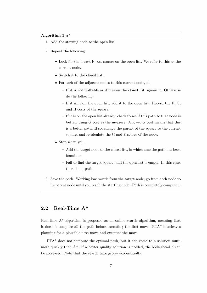
Algorithm 1 A*
1. Add the starting node to the open list
2. Repeat the following:
• Look for the lowest F cost square on the open list. We refer to this as the
current node.
• Switch it to the closed list.
• For each of the adjacent nodes to this current node, do
– If it is not walkable or if it is on the closed list, ignore it. Otherwise
do the following.
– If it isn’t on the open list, add it to the open list. Record the F, G,
and H costs of the square.
– If it is on the open list already, check to see if this path to that node is
better, using G cost as the measure. A lower G cost means that this
is a better path. If so, change the parent of the square to the current
square, and recalculate the G and F scores of the node.
• Stop when you:
– Add the target node to the closed list, in which case the path has been
found, or
– Fail to find the target square, and the open list is empty. In this case,
there is no path.
3. Save the path. Working backwards from the target node, go from each node to
its parent node until you reach the starting node. Path is completely computed.
2.2 Real-Time A*
Real-time A* algorithm is proposed as an online search algorithm, meaning that
it doesn’t compute all the path before executing the first move. RTA* interleaves
planning for a plausible next move and executes the move.
RTA* does not compute the optimal path, but it can come to a solution much
more quickly than A*. If a better quality solution is needed, the look-ahead d can
be increased. Note that the search time grows exponentially.
7
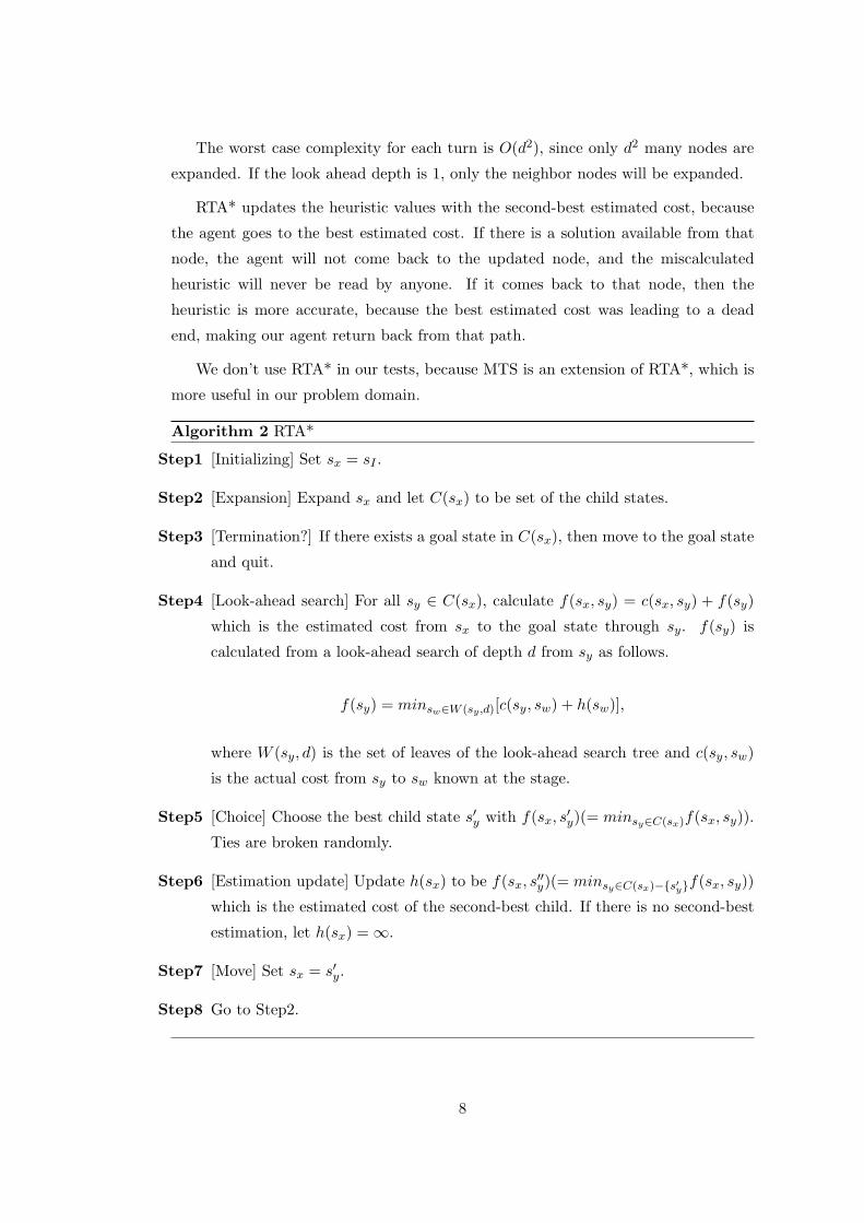
The worst case complexity for each turn is O(d2), since only d2 many nodes are
expanded. If the look ahead depth is 1, only the neighbor nodes will be expanded.
RTA* updates the heuristic values with the second-best estimated cost, because
the agent goes to the best estimated cost. If there is a solution available from that
node, the agent will not come back to the updated node, and the miscalculated
heuristic will never be read by anyone. If it comes back to that node, then the
heuristic is more accurate, because the best estimated cost was leading to a dead
end, making our agent return back from that path.
We don’t use RTA* in our tests, because MTS is an extension of RTA*, which is
more useful in our problem domain.
Algorithm 2 RTA*
Step1 [Initializing] Set sx = sI .
Step2 [Expansion] Expand sx and let C(sx) to be set of the child states.
Step3 [Termination?] If there exists a goal state in C(sx), then move to the goal state
and quit.
Step4 [Look-ahead search] For all sy ∈ C(sx), calculate f(sx, sy) = c(sx, sy) + f(sy)
which is the estimated cost from sx to the goal state through sy. f(sy) is
calculated from a look-ahead search of depth d from sy as follows.
f(sy) = minsw∈W (sy,d)[c(sy, sw) + h(sw)],
where W (sy, d) is the set of leaves of the look-ahead search tree and c(sy, sw)
is the actual cost from sy to sw known at the stage.
Step5 [Choice] Choose the best child state s′y with f(sx, s′y)(= minsy∈C(sx)f(sx, sy)).
Ties are broken randomly.
Step6 [Estimation update] Update h(sx) to be f(sx, s′′y)(= minsy∈C(sx)−{s′y}f(sx, sy))
which is the estimated cost of the second-best child. If there is no second-best
estimation, let h(sx) =∞.
Step7 [Move] Set sx = s′y.
Step8 Go to Step2.
8
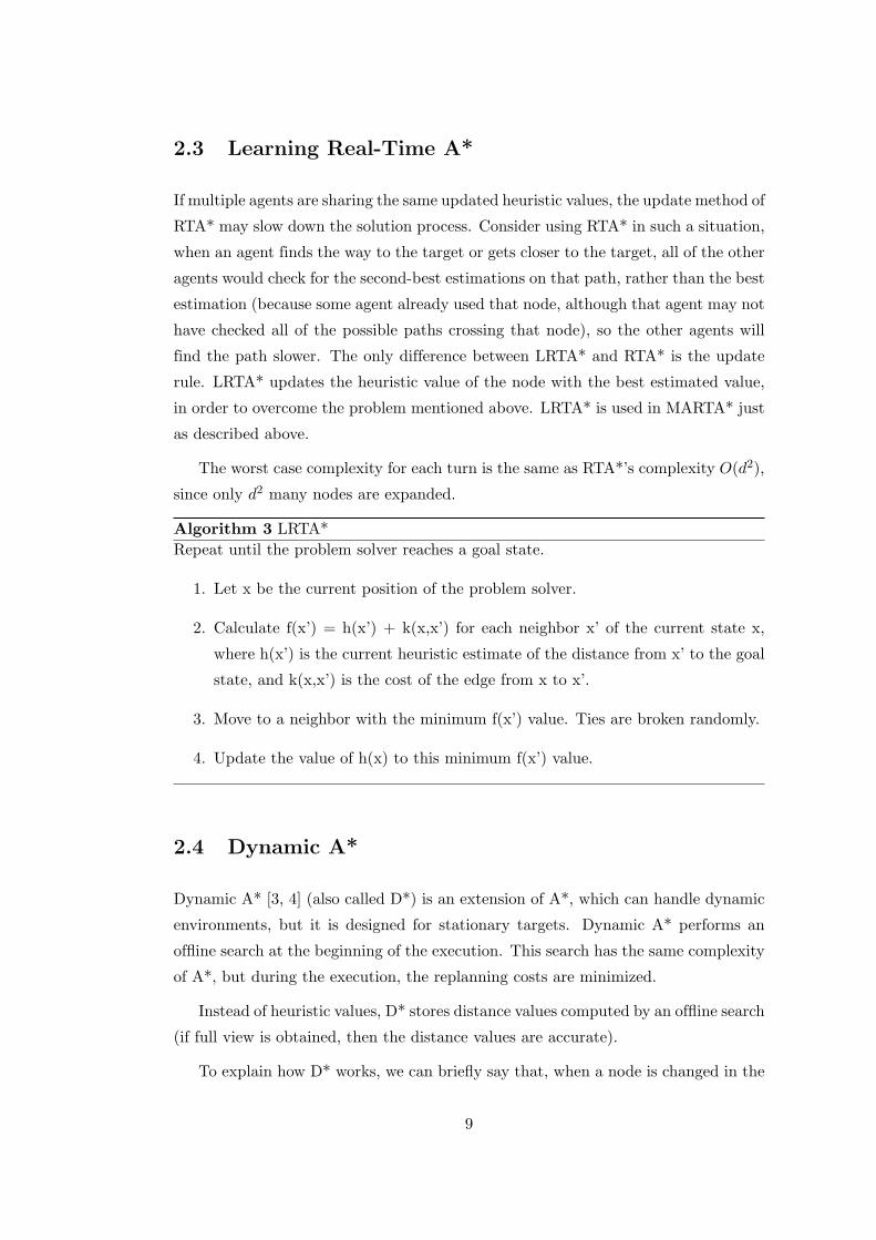
2.3 Learning Real-Time A*
If multiple agents are sharing the same updated heuristic values, the update method of
RTA* may slow down the solution process. Consider using RTA* in such a situation,
when an agent finds the way to the target or gets closer to the target, all of the other
agents would check for the second-best estimations on that path, rather than the best
estimation (because some agent already used that node, although that agent may not
have checked all of the possible paths crossing that node), so the other agents will
find the path slower. The only difference between LRTA* and RTA* is the update
rule. LRTA* updates the heuristic value of the node with the best estimated value,
in order to overcome the problem mentioned above. LRTA* is used in MARTA* just
as described above.
The worst case complexity for each turn is the same as RTA*’s complexity O(d2),
since only d2 many nodes are expanded.
Algorithm 3 LRTA*Repeat until the problem solver reaches a goal state.
1. Let x be the current position of the problem solver.
2. Calculate f(x’) = h(x’) + k(x,x’) for each neighbor x’ of the current state x,
where h(x’) is the current heuristic estimate of the distance from x’ to the goal
state, and k(x,x’) is the cost of the edge from x to x’.
3. Move to a neighbor with the minimum f(x’) value. Ties are broken randomly.
4. Update the value of h(x) to this minimum f(x’) value.
2.4 Dynamic A*
Dynamic A* [3, 4] (also called D*) is an extension of A*, which can handle dynamic
environments, but it is designed for stationary targets. Dynamic A* performs an
offline search at the beginning of the execution. This search has the same complexity
of A*, but during the execution, the replanning costs are minimized.
Instead of heuristic values, D* stores distance values computed by an offline search
(if full view is obtained, then the distance values are accurate).
To explain how D* works, we can briefly say that, when a node is changed in the
9
environment (it was assumed to be empty, but now there is an obstacle), D* checks
the validity of the distance value with the distance values of the neighbors of the
changing node. If a distance value is not valid anymore (because of the change in the
grid), that distance is recalculated (by a partial search).
When all of the distance values of the neighbors of the changed node is valid, D*
continues to execute the moves.
The computed path is optimal in the sense that the path which seems to be the
shortest path is computed. That path may turn out to have obstacles on the road,
so it may not be optimal.
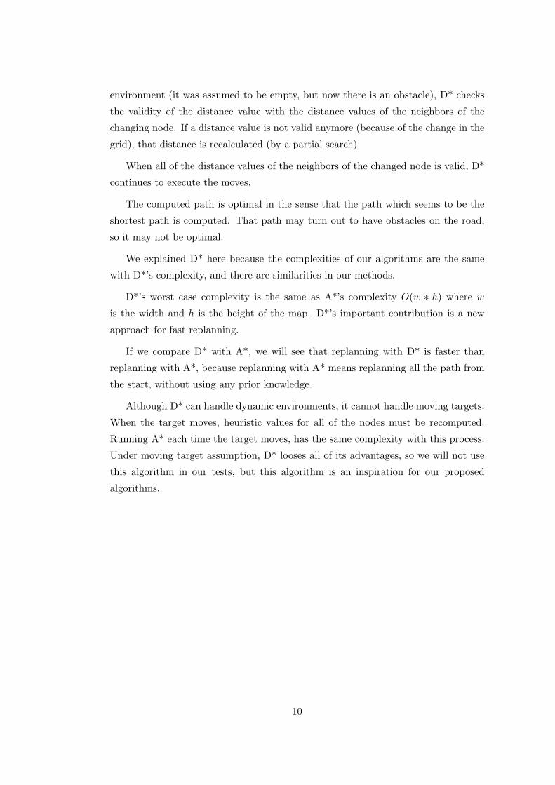
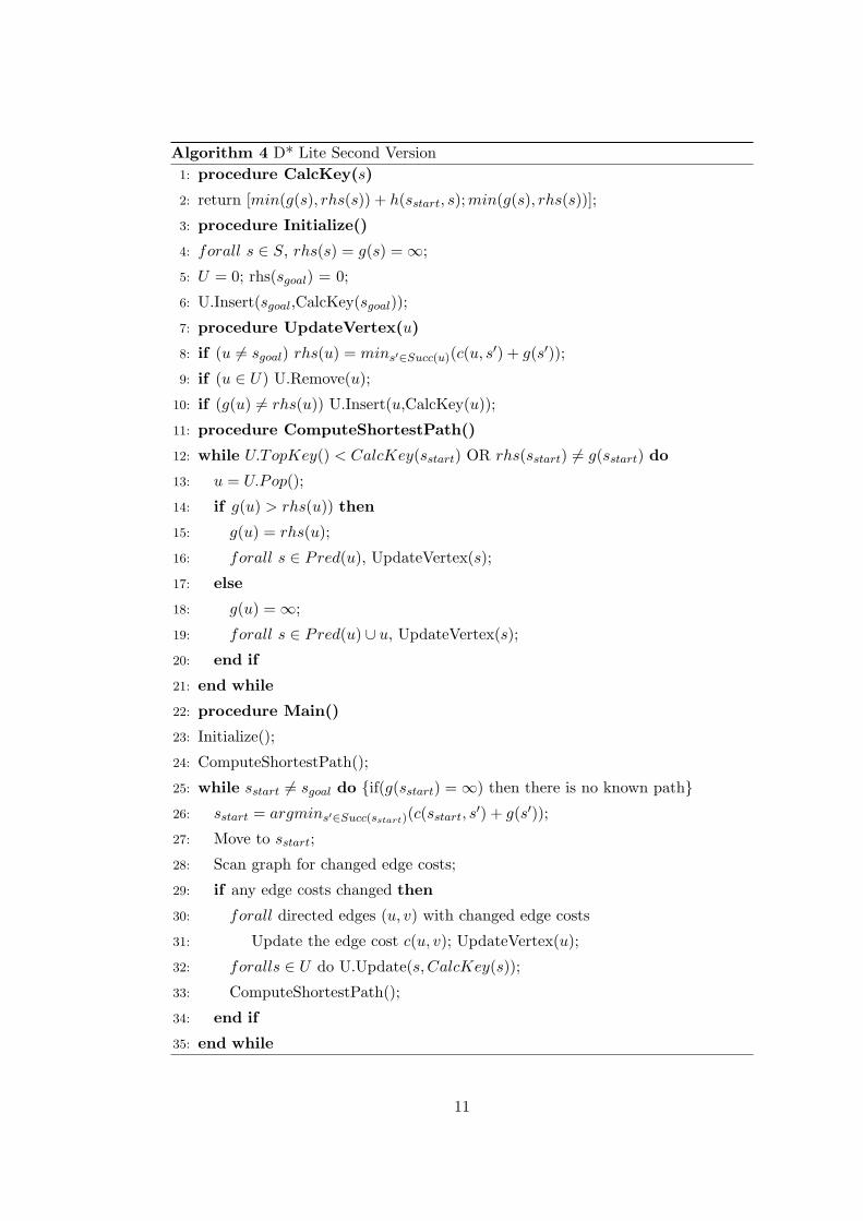
We explained D* here because the complexities of our algorithms are the same
with D*’s complexity, and there are similarities in our methods.
D*’s worst case complexity is the same as A*’s complexity O(w ∗ h) where w
is the width and h is the height of the map. D*’s important contribution is a new
approach for fast replanning.
If we compare D* with A*, we will see that replanning with D* is faster than
replanning with A*, because replanning with A* means replanning all the path from
the start, without using any prior knowledge.
Although D* can handle dynamic environments, it cannot handle moving targets.
When the target moves, heuristic values for all of the nodes must be recomputed.
Running A* each time the target moves, has the same complexity with this process.
Under moving target assumption, D* looses all of its advantages, so we will not use
this algorithm in our tests, but this algorithm is an inspiration for our proposed
algorithms.
10
Algorithm 4 D* Lite Second Version1: procedure CalcKey(s)
2: return [min(g(s), rhs(s)) + h(sstart, s);min(g(s), rhs(s))];
3: procedure Initialize()
4: forall s ∈ S, rhs(s) = g(s) =∞;
5: U = 0; rhs(sgoal) = 0;
6: U.Insert(sgoal,CalcKey(sgoal));
7: procedure UpdateVertex(u)
8: if (u 6= sgoal) rhs(u) = mins′∈Succ(u)(c(u, s′) + g(s′));
9: if (u ∈ U) U.Remove(u);
10: if (g(u) 6= rhs(u)) U.Insert(u,CalcKey(u));
11: procedure ComputeShortestPath()
12: while U.TopKey() < CalcKey(sstart) OR rhs(sstart) 6= g(sstart) do
13: u = U.Pop();
14: if g(u) > rhs(u)) then
15: g(u) = rhs(u);
16: forall s ∈ Pred(u), UpdateVertex(s);
17: else
18: g(u) =∞;
19: forall s ∈ Pred(u) ∪ u, UpdateVertex(s);
20: end if
21: end while
22: procedure Main()
23: Initialize();
24: ComputeShortestPath();
25: while sstart 6= sgoal do {if(g(sstart) =∞) then there is no known path}26: sstart = argmins′∈Succ(sstart)(c(sstart, s
′) + g(s′));
27: Move to sstart;
28: Scan graph for changed edge costs;
29: if any edge costs changed then
30: forall directed edges (u, v) with changed edge costs
31: Update the edge cost c(u, v); UpdateVertex(u);
32: foralls ∈ U do U.Update(s, CalcKey(s));
33: ComputeShortestPath();
34: end if
35: end while
11
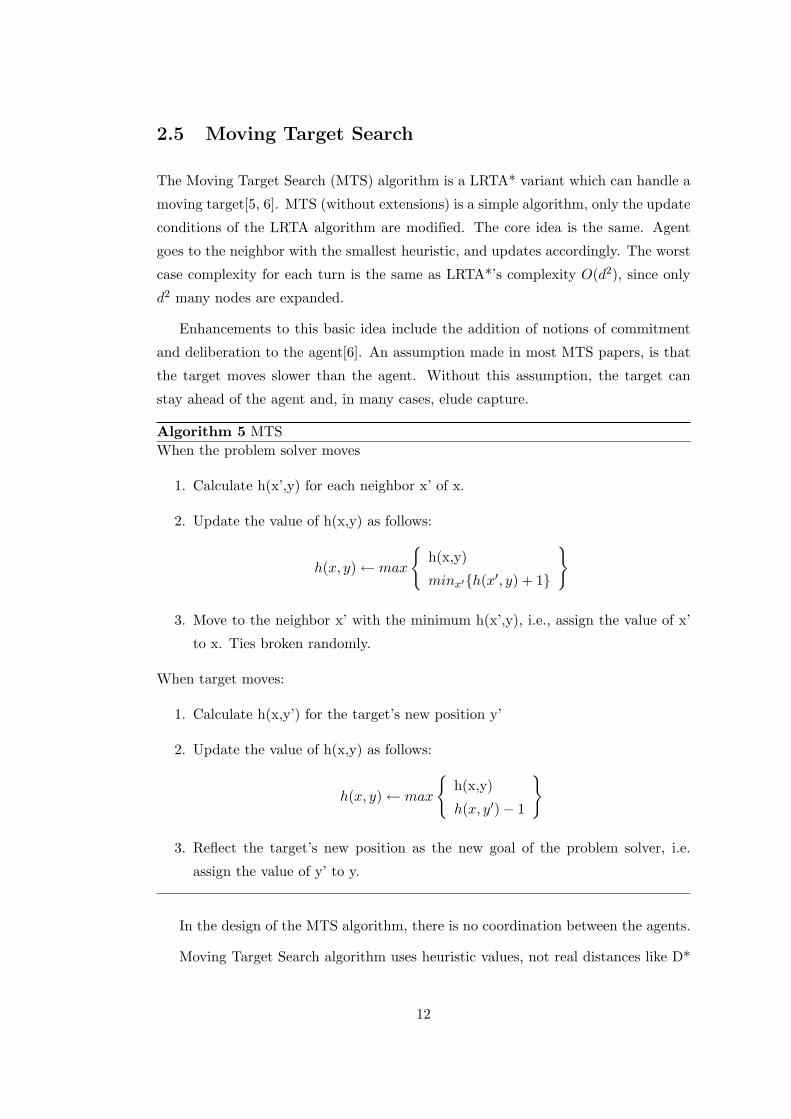
2.5 Moving Target Search
The Moving Target Search (MTS) algorithm is a LRTA* variant which can handle a
moving target[5, 6]. MTS (without extensions) is a simple algorithm, only the update
conditions of the LRTA algorithm are modified. The core idea is the same. Agent
goes to the neighbor with the smallest heuristic, and updates accordingly. The worst
case complexity for each turn is the same as LRTA*’s complexity O(d2), since only
d2 many nodes are expanded.
Enhancements to this basic idea include the addition of notions of commitment
and deliberation to the agent[6]. An assumption made in most MTS papers, is that
the target moves slower than the agent. Without this assumption, the target can
stay ahead of the agent and, in many cases, elude capture.
Algorithm 5 MTSWhen the problem solver moves
1. Calculate h(x’,y) for each neighbor x’ of x.
2. Update the value of h(x,y) as follows:
h(x, y)← max
{h(x,y)
minx′{h(x′, y) + 1}
}
3. Move to the neighbor x’ with the minimum h(x’,y), i.e., assign the value of x’
to x. Ties broken randomly.
When target moves:
1. Calculate h(x,y’) for the target’s new position y’
2. Update the value of h(x,y) as follows:
h(x, y)← max
{h(x,y)
h(x, y′)− 1
}
3. Reflect the target’s new position as the new goal of the problem solver, i.e.
assign the value of y’ to y.
In the design of the MTS algorithm, there is no coordination between the agents.
Moving Target Search algorithm uses heuristic values, not real distances like D*
12
algorithm. Using heuristic values takes less computation time each turn, but since the
values are not accurate (they converge too slowly) the agent’s path doesn’t look like an
intelligently planned path, because of the oscillation during the heuristic depression.
In order to get rid of heuristic depression, deliberation extension is developed for
Moving Target Search. To achieve shorter paths, we prefer to use real distances in
our tests, knowing that more time will be spent.
2.6 Multi-Agent Real-Time A*
Multi-Agent Real-Time A* [7] is a multi-agent version of RTA* where multiple agents
concurrently search and move to find a solution. The aim is to improve the quality
of the solution by increasing the number of agents engaged in the search. MARTA
is originally designed for stationary targets, so there is no search for any alternative
escape route, by which the target can evade. In MARTA algorithm, every agent
performs a modified RTA algorithm, and a LRTA algorithm simultaneously. The
heuristic values updated by the LRTA algorithm is shared between the agents. So
the heuristic conversion becomes faster with multiple agents, but every agent also
maintains their local heuristic table updated by the RTA algorithm, so that the
search time does not increase because of LRTA.
When an agent is trying to choose its next step by comparing the f values of
its neighbors, there may be more than one best node. In regular RTA* versions,
ties are broken randomly, but in MARTA, the organizational strategies are taken
into consideration in ties. If there is still a tie condition, then those ties are broken
randomly.
MARTA has 2 organizational strategies: repulsion and attraction.
Repulsion is expected to strengthen the discovering effect by scattering agents in
a wider search space. In contrast, attraction is expected to strengthen the learning
effect by making agents update estimated costs in a smaller search space more ac-
tively. When there are 2 nodes, whose f values are the same, MARTA with repulsion
chooses the node which is further away from the other agents, where MARTA with
attraction chooses the node which is closer to the other agents. Repulsion is used
in grid domains, where the discovering effect is more important than the learning
effect. Attraction is used in domains like 8-puzzle problem, where the learning effect
is more important than the discovering effect.
13
The worst case complexity for each turn is the same as LRTA*’s complexity
O(d2), since only d2 many nodes are expanded. If tie condition arises in a turn, the
distances between the other agents and the nodes in the tie condition are computed.
Generally the agent number is a small number, which is not necessary to mention
in the complexity calculations. Extreme numbers of agents are not usual in this
domain, so it may be neglected. To be accurate we should mention that the distance
computation in tie condition increases the worst case complexity to O(d2 ∗ a) where
a is the agent number. There are d2 expanded nodes, but the computation for each
node includes a− 1 distance computations.
Although this algorithm is not designed for our problem domain, we will combine
this algorithm’s repulsion cooperation technique with other algorithms (A* and MTS)
to create new algorithms for comparison.
2.7 Multi-Agent Moving Target Search
In [8] Goldenberg et al. proposed an algorithm for Multi-Agent Moving Target Search
problem. The original design of the MAMTS algorithm is capable of handling the
environments with partial visibility and partial communication.
MAMTS algorithm maintains a belief set for the target position. In each turn,
the belief set is updated with the possible positions of the target. If the target is
detected, the belief set is cleared. If the target is not in sight, the new possible
positions of the target are added to the belief set. The beliefs that turn out to be
wrong are eliminated. Then the belief set is filtered to find the corner nodes of
the belief set. These filtered corner nodes will be called as the filtered belief set.
The agents select their goals from this filtered belief set. Each agent computes the
minimum(distance to belief − (minimum distance between the belief and the other
agents)) for all of the possible goal nodes, and the node with the minimum value
is set as the goal of that agent. The goal selection step is the cooperation method
of MAMTS algorithm. Every agent selects its goal cooperatively. After the goal is
selected any search algorithm can be performed to navigate to the goal. The choice
of the algorithm is left to the implementer.
Figure 2.1 (left) illustrates the different belief sets. The agent (A) sees the target
(T) and then both of them move twice. The belief set is represented by the shaded
squares.
14
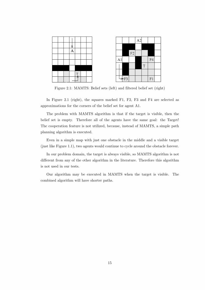
Figure 2.1: MAMTS: Belief sets (left) and filtered belief set (right)
In Figure 2.1 (right), the squares marked F1, F2, F3 and F4 are selected as
approximations for the corners of the belief set for agent A1.
The problem with MAMTS algorithm is that if the target is visible, then the
belief set is empty. Therefore all of the agents have the same goal: the Target!
The cooperation feature is not utilized, because, instead of MAMTS, a simple path
planning algorithm is executed.
Even in a simple map with just one obstacle in the middle and a visible target
(just like Figure 1.1), two agents would continue to cycle around the obstacle forever.
In our problem domain, the target is always visible, so MAMTS algorithm is not
different from any of the other algorithm in the literature. Therefore this algorithm
is not used in our tests.
Our algorithm may be executed in MAMTS when the target is visible. The
combined algorithm will have shorter paths.
15
Chapter 3
Multi-Agent Moving Target
Pursuit
3.1 Problem Description
The following paragraphs describe the experimental domain used in this thesis. The
domain can be extended to be more realistic. However, even the simplified domain
used here is quite challenging. The assumptions that can be relaxed are explained in
the future works section, in detail.
The test domain has the following properties:
1. Agents and target: There are multiple agents pursuing a single moving target.
The number of agents differs between 2 to 4 in our tests.
2. Grid: The grid is m ∗ n in size and it is static. All agents and the target have
complete knowledge of the grid topology. These assumptions can be relaxed.
Two types of grids are generated for testing:
• Maps with random obstacles
• Hand-crafted maps
Maps with random obstacles are classified in two groups. The maps with big
obstacles, and the ones with small obstacles.
3. Moves: The target and the agents can move horizontally, vertically or diagonally
(8 neighborhood grid domain). All the moves have the same cost. Although
16
this property is not realistic, it is easier to implement, easier to simulate and
already used in some computer games like Civilization and its derivatives[9].
This assumption can be changed. Diagonal moves may cost more, but this envi-
ronment configuration is in favor of the algorithms that we use for comparison.
The tie condition has a higher probability when all the possible moves have the
same cost.
Generally, nodes in the MTS tests have 4 neighbors (diagonal moves are not
permitted). But with this configuration, the pursuit gets longer, and when the
target and the agent move with the same speed, depending on the grid topology,
it may be impossible for one agent to catch the target. The target doesn’t even
need an obstacle to move forever in a loop.
4. At each time step, the target moves first, then the agents next.
5. Multiple agents are allowed to occupy the same square at any instance in time.
6. Starting position: Agents start at the same corner of the map, next to each
other. Target is positioned randomly.
7. Vision and communication: The agents and target are given full vision in our
experiments, so every one has complete information. Everyone knows the posi-
tions of the other agents and the target. Communication is allowed between all
agents. We choose to give every one, all the information, to get better results.
8. Objective: The multiple agents have to capture the target in the fewest possible
moves. Capture is defined as being on the same square with the target.
3.2 Agent Design
Calculating real distances takes more time, but gives us better paths and even the
total processing time may be smaller, just like D* may be faster than RTA*. Both
of the algorithms proposed below are not RTA* derivatives, they are much similar to
A* and D*.
3.2.1 Moving Target Algorithm
In order to test our agent algorithms, we need a good target algorithm, because
the pursuit length and success is heavily dependant on the targets decisions. Simple
17
algorithms like avoiding (going the opposite direction of the nearest agent) or random
behavior are insufficient for our tests. We need a successfully escaping target to test
the cooperation of the agents. To perform more realistic tests we required a target
algorithm, which can survive as long as it could.
Ties are broken randomly. This random effect changes the escape route, and
therefore changes the survival length of the target. While traveling to that location,
the agent positions change, making us repeat this computation in every turn, so that
the target does not go to the corner of the map, and stay there unless it is cornered.
It moves to a new position while the agents are getting closer. When the target is
cornered, it finds the location which it will survive the longest, and waits in that spot
(some dead end in the grid).
After we choose the best location for the target, we do not check if there is a safe
path from the current location to the target location, because we only expand safe
nodes, so there is a safe path. Therefore the algorithm runs fast when the target is
cornered, because there is limited number of safe nodes to expand.
The algorithm computes the shortest paths for all of the agents, so the worst
case complexity of a turn is O(n ∗m ∗ a), where a is the total number of agents and
the target. This data is shared with the agents for purposes of speed, and cached
for future use. Since the grid is static and fully visible, the cached values can be
trusted in the future turns, no extra check or maintenance is needed. The target
algorithm does not need to compute all of this data. It is calculated for all of the
agents including the target. The target only needs the distance values to its positions,
so if we want to compute the complexity of the target only, the complexity would be
O(n ∗m).
If all of the agent positions are met before (the distances were cached), the com-
putation of the shortest paths complexity is O(1) for that turn. This is the best
case for the shortest paths computation. In this case, the rest of the target decision
method becomes the important variable for the algorithms complexity. In the worst
case, the target would expand half of the open nodes, which gives us the complexity
of O(n ∗m). Best case would occur when the target is cornered, where one turn is
left before the capture and the target don’t have any safe node, so there will be no
computation, which gives us the complexity of O(1).
Although our target algorithm is not capable of detecting cycles, and using them,
it is a good runner. Since their speeds are the same with the agent, the target does not
18
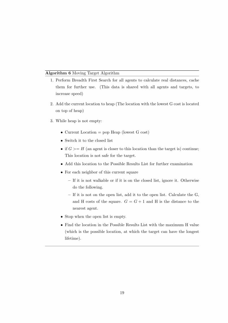
Algorithm 6 Moving Target Algorithm
1. Perform Breadth First Search for all agents to calculate real distances, cache
them for further use. (This data is shared with all agents and targets, to
increase speed)
2. Add the current location to heap (The location with the lowest G cost is located
on top of heap)
3. While heap is not empty:
• Current Location = pop Heap (lowest G cost)
• Switch it to the closed list
• if G >= H (an agent is closer to this location than the target is) continue;
This location is not safe for the target.
• Add this location to the Possible Results List for further examination
• For each neighbor of this current square
– If it is not walkable or if it is on the closed list, ignore it. Otherwise
do the following.
– If it is not on the open list, add it to the open list. Calculate the G,
and H costs of the square. G = G + 1 and H is the distance to the
nearest agent.
• Stop when the open list is empty.
• Find the location in the Possible Results List with the maximum H value
(which is the possible location, at which the target can have the longest
lifetime).
19
get stuck, if it cycles around an obstacle. On many tests this target algorithm evaded
the capture of the known agent algorithms. After some time over these successful
escapes, all of the agents were following the target on the same direction. There was
absolutely no coordination between the agents.
Possible Improvements
If the map has long paths with dead ends, the algorithm may choose to go to that
dead end, although there is a cyclic path which it can take and survive longer. This
property of the algorithm needs improvement.
3.2.2 Coordinated Agent Algorithm
We now present our Coordinated Agent Algorithm: named as Multi-Agent Moving
Target Pursuit, which is the main contribution of this thesis.
Here, how it works: Consider a path between an agent and a target. We calculate
the midpoint of that path. If the agent is the closest agent to the calculated point,
then it is the most suitable agent to guard the related path. In order to find the
most suitable path for an agent, we compute the paths to the target. Since we know
the real distances, this computation is easy. We perform a derivative of A* search.
When we are at the midpoint of a path, we check whether the referred agent is the
closest agent to that point. If our agent is the closest one, we stop computation,
setting the goal of the agent as this point, and the agent moves to its appropriate
neighbor, which will lead to that midpoint. We don’t need to check the rest of the
path, because we use the real values, so we know there is a path to the target with
the specified length. We also do not need to check for the other agents for the rest
of the path. There may be agents closer to the nodes in the rest of the path, but it
does not mean that those agents can guard the path better than our agent.
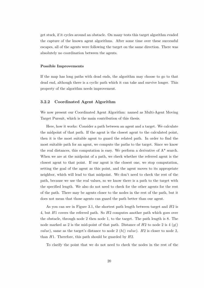
As you can see in Figure 3.1, the shortest path length between target and H2 is
4, but H1 covers the referred path. So H2 computes another path which goes over
the obstacle, through node 2 then node 1, to the target. The path length is 8. The
node marked as 2 is the mid-point of that path. Distance of H2 to node 2 is 4 (g()
value), same as the target’s distance to node 2 (h() value). H2 is closer to node 2,
than H1. Therefore, this path should be guarded by H2.
To clarify the point that we do not need to check the nodes in the rest of the
20
P
1
2
-
H2¡¡µ
H1 -
Figure 3.1: The Mid-Point Explanation
path; lets check for a node that is beyond the mid-point (e.g. node marked as 1) on
the computed path of H2, and see how it will mislead us. H1 is closer to the node
marked as 1 (5 < 6) than H2. Although H1 is closer, it is obvious that he cannot
guard that path, better than H2. Therefore, the nodes beyond the midpoint should
not be checked for the closest agent, because this information does not mean that
those agents can guard those paths, since the target may be closer to that point than
all of the agents.
We make this calculation at every turn. If the agent does not recompute and
follow its precomputed path, the time spent at each turn will be reduced, but the
total distance and the number of turns will increase.
If the agent cannot find any path, meaning either there is no path, or the other
agents are already guarding all of the paths, then the agent may be considered un-
needed. In such a case the agent may stop, but instead of stopping, we let our agent
follow the shortest path to the target. Although there is another agent already guard-
ing the related route, our agent, as a second one, may come in handy at the same
route.
Consider the case: if the target starts to cycle around an obstacle, it would be
impossible for only one agent guarding that route, to succeed on his own. When the
target completes the tour around the obstacle, he may start to walk on the path,
once guarded by the agent, who has fallen behind now. At that point, the second
agent, who choose this path instead of stopping, would start to run towards the target
(since the first agent would be closing the other direction). If the agent followed the
shortest path, instead of stopping, he would be closer to the target. Hence when an
agent cannot find an alternative path to guard, we let him follow the shortest path,
which is already guarded. This behavior takes an insignificant computation time,
but it may shorten the overall pursuit time significantly.
Different agents should not try to guard the same escape route, but it is difficult
21
P
6
H2 H1¡¡µ
(a) H2 is not needed
P
6
H26
H1 -
(b) H2 is needed
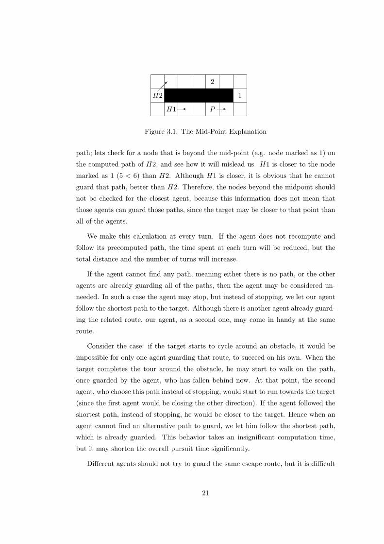
Figure 3.2: MAMTP Example
to differentiate the routes, especially if you are using heuristic values, which does not
utilize the grid information. Two agents may have planned two different paths, but
one of them may be able to guard both of those paths without changing its original
path. If there is an obstacle separating the paths, then both of those agents may be
necessary for guarding those paths.
As you can see in Figure 3.2(a) the agent H1 cornered the target P , so H2 cannot
find a path that H1 does not guard. Heuristic values are valid for this grid, because
there isn’t any obstacle in the map.
If there were an obstacle separating the paths, the heuristic values become un-
sound. As you can see in Figure 3.2(b) the agent H1 couldn’t corner the target P
just by himself, and H2 computes a path that H1 cannot guard. The agent positions
and the target position are the same, but an obstacle changes the paths.
The heuristic functions cannot utilize environmental information. If we used
heuristic values instead of real distances, H2 would not be able to find any alternative
escape route in Figure 3.2(b) (even if there is one, which he should guard), so he would
choose to follow the other agent, since this is the shortest path.
The complexity of our agent algorithm is similar to the target algorithm. It
also needs to compute the shortest paths to other agents. Therefore the worst case
complexity is O(n ∗m ∗ a). If all the paths are already in the cache, then the rest of
the method has a worst case (target is too far, expanded node number is written in
terms of n ∗m) complexity of O(n ∗m) and a best case (the target is about to be
captured) complexity of O(1).
22
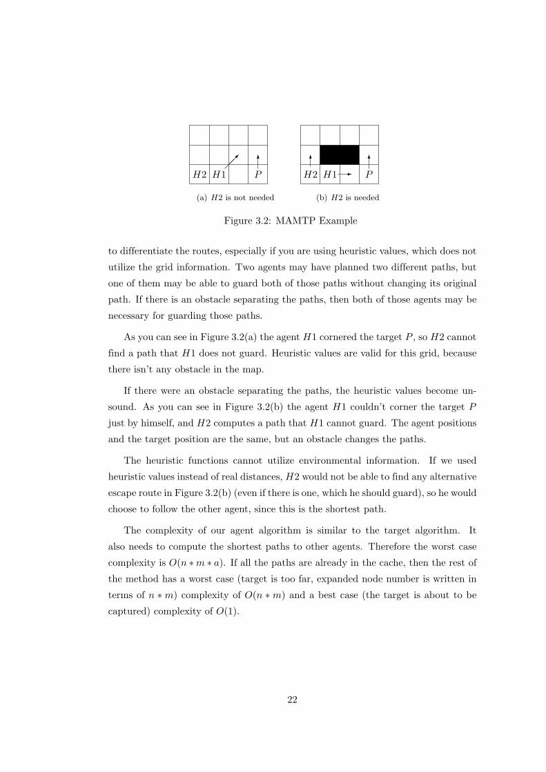
Algorithm 7 Multi-Agent Moving Target Pursuit AlgorithmRequire: si {Initial location} target {Target Location}1: for all agents do
2: if Real Distances of agent location is not calculated yet then
3: Calculate Real Distances from this agent to other points of the grid
4: end if
5: end for
6: Heap.push(si,RealDistanceToPrey(si),0) {Arguments: Location, H, G}7: while Heap 6= Empty do
8: {Let x be the Current Location}9: x⇐ PopHeap() {Location with the lowest F (= G + H) value is popped}
10: x is closed
11: if x = target then
12: break {Path found}13: end if
14: if G >= H then {This is the midpoint between the target and the agent}15: if this agent is the closest agent to this mid-point then
16: break {Path found}17: end if
18: end if
19: for all Neighbors of x do {Let the neighbor be N}20: if N is not valid OR not walkable OR on the closed list then
21: continue
22: end if
23: if N is not opened already then
24: Open N
25: Set x as the parent of N {Parents are used to find the path}26: Heap.push(N ,RealDistanceToPrey(N),x.G+1)
27: end if
28: end for
29: end while
30: if No path Found then
31: Follow the path to the target
32: else if Path found then
33: Follow the path
34: end if
23
Chapter 4
Experimental Results
4.1 Test Environment
Our target algorithm is used for planning the target movement. The computation
of the target’s escape route is affected by random criterions and the agent positions
which are also affected by random values. Since the path lengths and the pur-
suit success rate is strongly dependant on the targets escape route, a few test runs
would not be enough for making decisions. Therefore, we have run each environment
configuration (same map, with same initial agent positions and same initial target
position) 100 times, and it can be seen from the results that the algorithms doesn’t
always give the same result.
Length limit for the maximum pursuit is set as 10 ∗ (n + m). If the target is still
alive after the limit has passed, we stop the execution.
Hand-crafted maps have different map sizes varying from 10x10 to 35x35. The
randomly generated maps have sizes of 10x10, 20x20, and 30x30, with obstacle ratios
of 10%, 20%, and 30%. The randomly generated maps are grouped in two classes: the
maps with big obstacles and the ones small obstacles (independent from the obstacle
ratio). The maps with small obstacles are generated with 1x1 building blocks of
obstacles. The maps with bigger obstacles are generated with 2x2 building blocks of
obstacles. The obstacle ratios are the same. In the maps with small obstacles, the
obstacles are scattered around the grid. They are more dispersed. The obstacles in
the other maps are united, they form bigger obstacles.
We have 10 maps for each random configuration of maps. As a total, we have 180
random generated maps (90 maps with smaller obstacles and 90 maps with bigger
obstacles), and 30 hand generated maps. We have run each algorithm a hundred
24
times on each map, so as a total we executed 105000 runs.
Since we want to test the coordination between the agents, we want to eliminate
the chance effects in our tests. We also require the best performance from our target,
so that any effect caused by the deficiency of the target algorithm would be elimi-
nated. It was mentioned that our target algorithm has a weakness about the dead
ends. Even only one agent may be enough for capture on maps with long dead ends.
These maps are not appropriate for testing the coordination between the agents.
In order to gain the maximum performance from our target algorithm, specific
maps, which do not contain dead ends at the corners, are generated. By this strategy,
we force our target to make use of the cycles in the map.
If the agents are placed far from each other, they guard different escape routes
without cooperating. Therefore agents are placed at the same corner of the map, so
that they have to cooperate to guard different escape routes. The target is placed
somewhere in the middle of the map. (This does not affect the result significantly.
The locations and the results differ slightly)
The test metrics used in the tests are: average path length over all of the runs,
average path length over the successful runs, success rate of the algorithm, and total
CPU time spent during the pursuits (both successful and unsuccessful ones).
In the calculation of the average path length over all of the runs, the maximum
limit is used as the path length, at which the agents fail to capture the target. So
when the success rate is 0%, the result becomes 100 ∗ 10 ∗ (n + m), which appears
to be too large. Since most of the current algorithms have a low success rate in the
tests, we choose to print the average path length over the successful runs instead
of average path length over all of the runs in the tables, in order to achieve better
perception.
The average path length over all of the runs, may be a metric, which can be used
on its own. But the average path length over the successful runs may be mislead-
ing without the success rate. Since some algorithms are successful only in a small
percentage of the runs, in which the path lengths may be short. These algorithms
may seem to be better than the other algorithms in terms of average path length
over successful runs, but the other algorithms perform better than these algorithms.
According to the target’s moves, and the random effect, the pursuit may become a
short one, and these algorithms may capture the target only in these short runs. But
since the other algorithms with higher success ratios, are also successful in longer
25
pursuits, their average pursuit length gets higher. Therefore, this metric should be
considered together with the success ratio of the algorithms.
Finally, the test algorithms used in the tests are:
Multi-Agent Moving Target Pursuit: Our algorithm that we introduced in Sec-
tion 3.2.2. (Abbreviated as MAMTP in some small figures)
MTS: Regular Moving Target Search algorithm, described in Section 2.5.
MTS with Repulsion: Since there is no coordination between the agents in regu-
lar MTS algorithm, we modified the MTS algorithm and added the same repulsion
organization strategy used in MARTA*. So there is minimal cooperation between
the agents (which is insufficient). When there are possible neighbor nodes with equal
distances to the target, the agent prefers the path which is further from the other
agents. (Abbreviated as MTSRep in some small figures)
A*: This is the regular A* algorithm, described in Section 2.1. The agents
compute all of the path again after each move.
A* with Repulsion: Since there is no coordination between the agents in regular
A* algorithm, we modified the A* algorithm and added the same repulsion organi-
zation strategy used in MARTA*. (Abbreviated as Arep in some small figures)
4.2 Test Results
If the map does not have any dead ends that the target may fall into (which is the
case in the test maps), coordination between the agents is mandatory for the capture.
As predicted before the algorithms in the literature that we used for comparison
cannot utilize the advantage of multi-agents as good as they should. As a result they
cannot capture the target in most of the hand made maps. The average success ratios
are given in the lines of the Table 4.1.
The obvious result of the tests is that the proposed algorithm has a higher success
ratio in all of the tests. Our algorithm successfully captured the target in all of
the tests run on the generated maps. In Table 4.1 you can see that our algorithm
failed on some of the tests run on two hand-crafted maps (11 and 19), but the other
algorithms had a lower success ratio on the same maps, so our algorithm can still be
called successful on these maps. Since the agents have the same speed as the targets,
there are maps that are not solvable by just 2 agents, but this was not the reason of
26
the mentioned failures.
When we take a closer look at the failures, we recognize that our algorithm has
a handicap. Although stopping is an option for our agents, it is never chosen. Our
algorithm always computes a path, and move on that path, but there are times that
an agent must stop, and wait for the other agent to get closer to the target. In the
above-mentioned failures, we realize that the agents who are closer to the target,
always chases without stopping, and the other agents try to block the alternative
escape route. But before an agent can block a route, the target heads for another
route, so the agent goes for the other route, but he is always late. (When he is not
late, that run is among the successful ones)
Although our algorithm did not fail in all of the test runs of a map, a special
map can be crafted on which our algorithm will always fail. This situation is not a
common situation, so a situation like this didn’t come up in a randomly generated
map. But improvement is needed, so that the success rates and also the path lengths
will be improved.
Our algorithm seems to have longer path lengths than MTS-Repulsion on some
tests These results can be seen in Table 4.2 on maps 7 & 10 and on the average.
On maps with 10% obstacle ratio with small obstacles, our algorithm is not needed.
Even A* algorithm can capture the target. We can see that cooperation is not needed
in this test case. When we take a closer look at these tests, we see that the target
cannot hide behind any obstacle. There is no obstacle big enough which the target can
utilize. The target goes to the further corner of the map, and waits for the capture.
But if the obstacles are bigger with the same map size and the same obstacle ratio,
the success ratio of the other algorithms start to fall. This can be seen in Figure 4.5
and Table 4.11. So we can see even if the obstacle ratio is 10%, if the target can
find obstacles big enough to utilize, he can evade capture, but it could not evade our
algorithm in any of the randomly generated maps.
As the obstacle ratio increases, we follow that the success rates of other algorithms
start falling. This tendency is obvious in Figure 4.2. When the obstacle ratio is 30%,
A* fails with a percentage of 66%, and regular MTS, performs better than the A*-
Repulsion. When we investigate, we see that A* and A* repulsion can always follow
the target. But this ability is not always useful. Although MTS tries to do the
same, it cannot follow as good as A*. The mistakes that MTS makes in the chase
becomes an advantage for MTS. The A* and A*-Repulsion agents follow almost the
same paths with their team mates. MTS agents cannot follow the same path. Even
27
on the tests that failed, they generally split up, without any purpose. The heuristics
depressions of MTS become an advantage over A* variations.
Figures 4.5 through 4.7 shows us that as the map size increases, the success rates
of other algorithms fall, while our algorithm’s success rate is independent of these
parameters. The other algorithms can succeed better in small maps with few scat-
tered obstacles, and they start to fail as the map grows, the obstacle ratio increases,
and the obstacles become bigger. So our algorithm is needed, because the other
algorithms only succeed in a small amount of maps.
The regular MTS algorithm, which can suffer from heuristic depressions, may
solve some of the problems above with a little help of luck. Since this algorithm cannot
chase the target closely, because of the heuristic depressions, the agents may be set
apart from each other, without an effort of cooperation. Sometimes this separation
of the agents may result in cornering the target. In the tests MTS performed even
better than the A* with Repulsion. But, we should state that this result is not to be
trusted. This is not a planned outcome of the algorithm, therefore not reliable, it is
highly aleatory, and the total pursuit paths are much higher than other algorithms.
MTS-Repulsion naturally takes more advantage of these split ups. So it performs
better than the other algorithms in the literature. Naturally A* performs the worst
in all of the test cases.
Although the MTS algorithms split up, this behavior is not planned according to
the target, so MTS-Repulsion cannot perform as good as MAMTP.
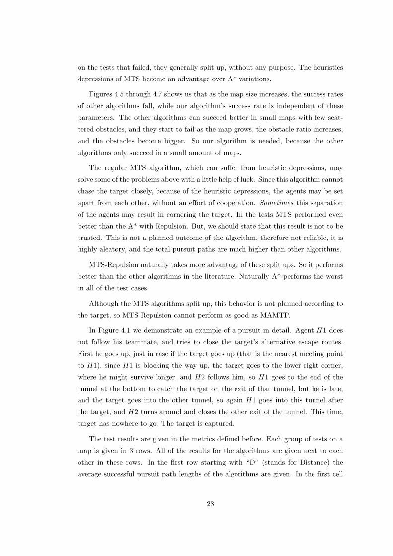
In Figure 4.1 we demonstrate an example of a pursuit in detail. Agent H1 does
not follow his teammate, and tries to close the target’s alternative escape routes.
First he goes up, just in case if the target goes up (that is the nearest meeting point
to H1), since H1 is blocking the way up, the target goes to the lower right corner,
where he might survive longer, and H2 follows him, so H1 goes to the end of the
tunnel at the bottom to catch the target on the exit of that tunnel, but he is late,
and the target goes into the other tunnel, so again H1 goes into this tunnel after
the target, and H2 turns around and closes the other exit of the tunnel. This time,
target has nowhere to go. The target is captured.
The test results are given in the metrics defined before. Each group of tests on a
map is given in 3 rows. All of the results for the algorithms are given next to each
other in these rows. In the first row starting with “D” (stands for Distance) the
average successful pursuit path lengths of the algorithms are given. In the first cell
28
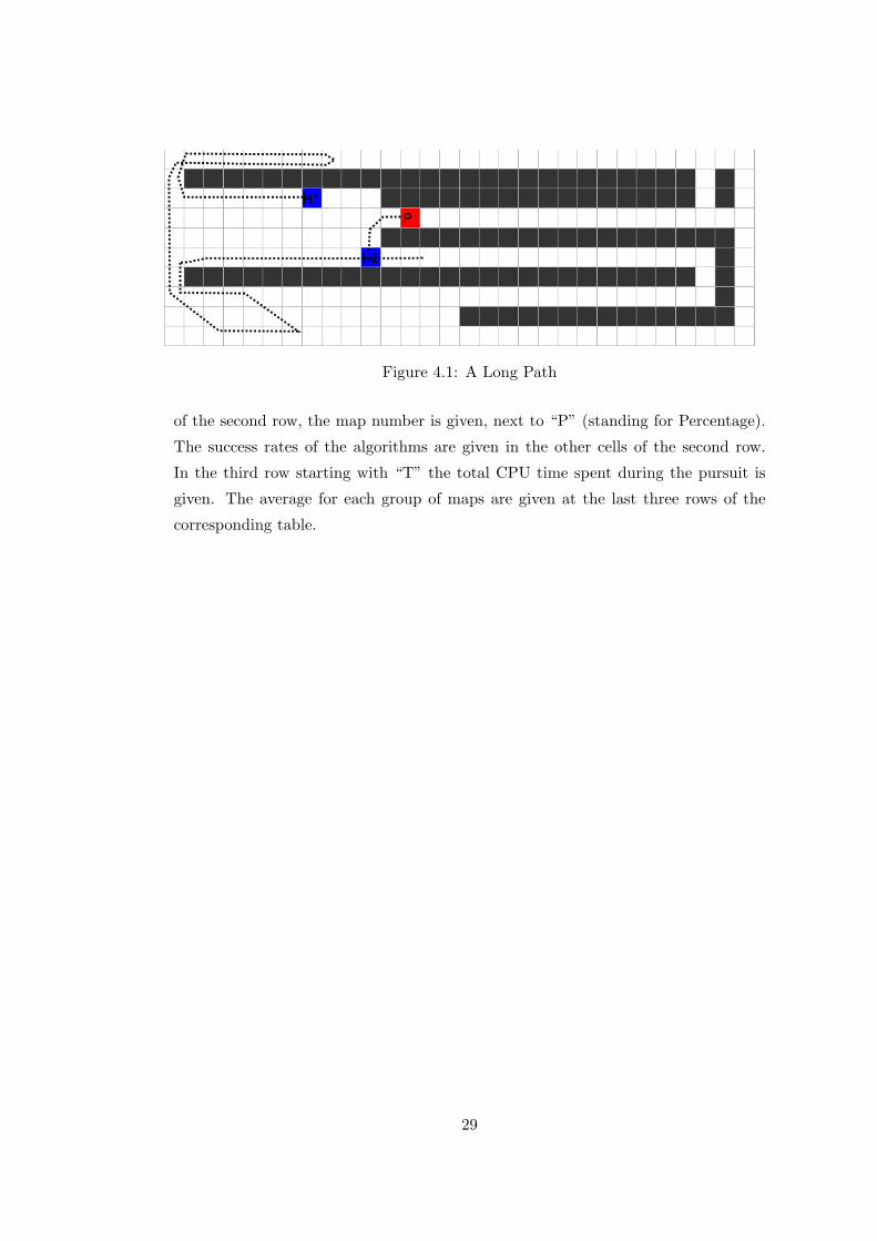
Figure 4.1: A Long Path
of the second row, the map number is given, next to “P” (standing for Percentage).
The success rates of the algorithms are given in the other cells of the second row.
In the third row starting with “T” the total CPU time spent during the pursuit is
given. The average for each group of maps are given at the last three rows of the
corresponding table.
29
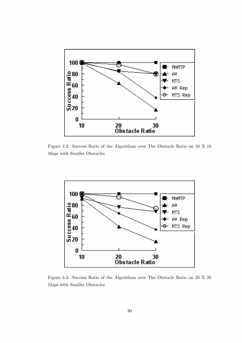
Figure 4.2: Success Ratio of the Algorithms over The Obstacle Ratio on 10 X 10
Maps with Smaller Obstacles
Figure 4.3: Success Ratio of the Algorithms over The Obstacle Ratio on 20 X 20
Maps with Smaller Obstacles
30
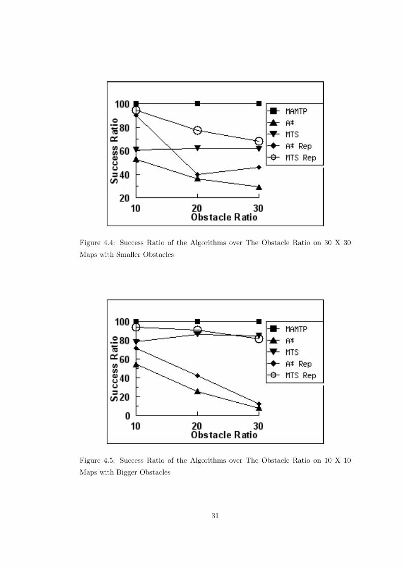
Figure 4.4: Success Ratio of the Algorithms over The Obstacle Ratio on 30 X 30
Maps with Smaller Obstacles
Figure 4.5: Success Ratio of the Algorithms over The Obstacle Ratio on 10 X 10
Maps with Bigger Obstacles
31
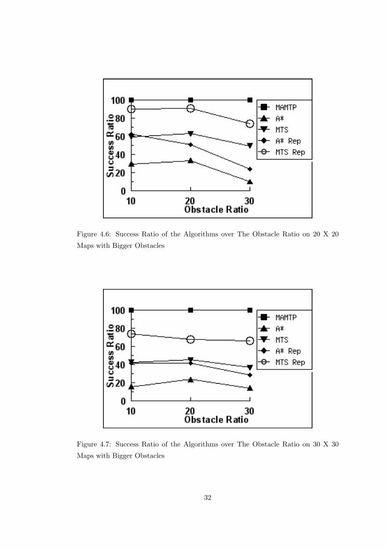
Figure 4.6: Success Ratio of the Algorithms over The Obstacle Ratio on 20 X 20
Maps with Bigger Obstacles
Figure 4.7: Success Ratio of the Algorithms over The Obstacle Ratio on 30 X 30
Maps with Bigger Obstacles
32
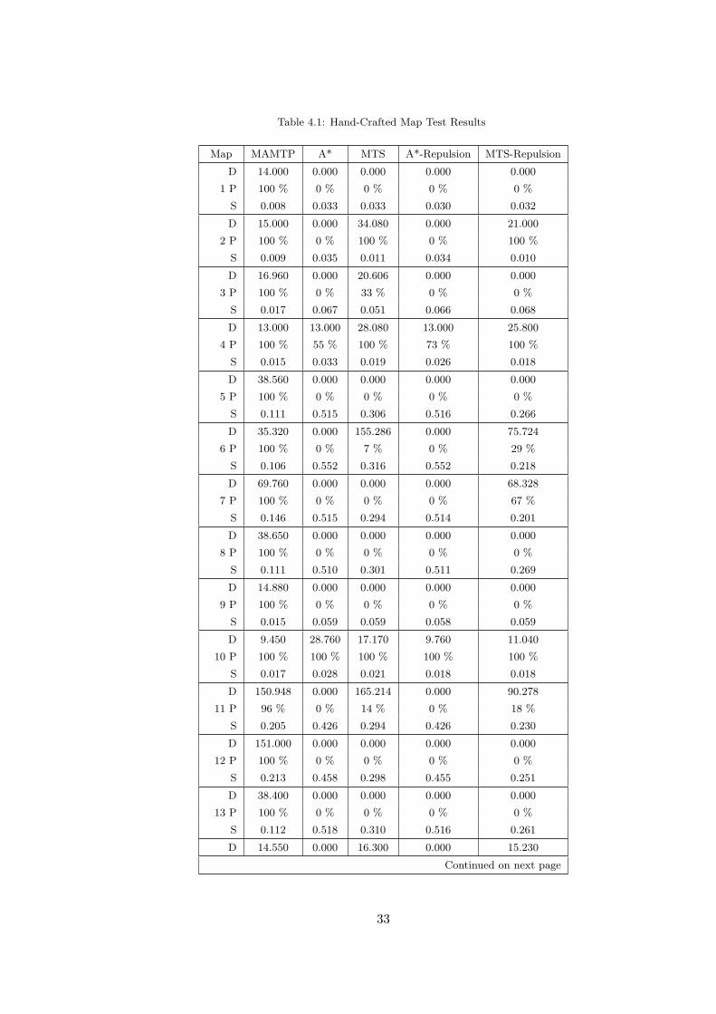
Table 4.1: Hand-Crafted Map Test Results
Map MAMTP A* MTS A*-Repulsion MTS-Repulsion
D 14.000 0.000 0.000 0.000 0.000
1 P 100 % 0 % 0 % 0 % 0 %
S 0.008 0.033 0.033 0.030 0.032
D 15.000 0.000 34.080 0.000 21.000
2 P 100 % 0 % 100 % 0 % 100 %
S 0.009 0.035 0.011 0.034 0.010
D 16.960 0.000 20.606 0.000 0.000
3 P 100 % 0 % 33 % 0 % 0 %
S 0.017 0.067 0.051 0.066 0.068
D 13.000 13.000 28.080 13.000 25.800
4 P 100 % 55 % 100 % 73 % 100 %
S 0.015 0.033 0.019 0.026 0.018
D 38.560 0.000 0.000 0.000 0.000
5 P 100 % 0 % 0 % 0 % 0 %
S 0.111 0.515 0.306 0.516 0.266
D 35.320 0.000 155.286 0.000 75.724
6 P 100 % 0 % 7 % 0 % 29 %
S 0.106 0.552 0.316 0.552 0.218
D 69.760 0.000 0.000 0.000 68.328
7 P 100 % 0 % 0 % 0 % 67 %
S 0.146 0.515 0.294 0.514 0.201
D 38.650 0.000 0.000 0.000 0.000
8 P 100 % 0 % 0 % 0 % 0 %
S 0.111 0.510 0.301 0.511 0.269
D 14.880 0.000 0.000 0.000 0.000
9 P 100 % 0 % 0 % 0 % 0 %
S 0.015 0.059 0.059 0.058 0.059
D 9.450 28.760 17.170 9.760 11.040
10 P 100 % 100 % 100 % 100 % 100 %
S 0.017 0.028 0.021 0.018 0.018
D 150.948 0.000 165.214 0.000 90.278
11 P 96 % 0 % 14 % 0 % 18 %
S 0.205 0.426 0.294 0.426 0.230
D 151.000 0.000 0.000 0.000 0.000
12 P 100 % 0 % 0 % 0 % 0 %
S 0.213 0.458 0.298 0.455 0.251
D 38.400 0.000 0.000 0.000 0.000
13 P 100 % 0 % 0 % 0 % 0 %
S 0.112 0.518 0.310 0.516 0.261
D 14.550 0.000 16.300 0.000 15.230
Continued on next page
33
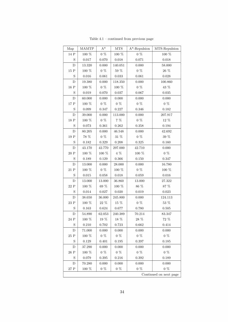
Table 4.1 – continued from previous page
Map MAMTP A* MTS A*-Repulsion MTS-Repulsion
14 P 100 % 0 % 100 % 0 % 100 %
S 0.017 0.070 0.018 0.071 0.018
D 13.320 0.000 140.051 0.000 58.000
15 P 100 % 0 % 59 % 0 % 26 %
S 0.016 0.061 0.033 0.061 0.028
D 19.380 0.000 118.350 0.000 100.860
16 P 100 % 0 % 100 % 0 % 43 %
S 0.019 0.070 0.037 0.067 0.035
D 60.000 0.000 0.000 0.000 0.000
17 P 100 % 0 % 0 % 0 % 0 %
S 0.099 0.347 0.227 0.346 0.182
D 39.000 0.000 113.000 0.000 207.917
18 P 100 % 0 % 7 % 0 % 12 %
S 0.073 0.361 0.262 0.358 0.194
D 80.205 0.000 46.548 0.000 42.692
19 P 78 % 0 % 31 % 0 % 39 %
S 0.182 0.329 0.208 0.325 0.160
D 43.170 42.770 297.000 42.710 0.000
20 P 100 % 100 % 4 % 100 % 0 %
S 0.189 0.129 0.366 0.150 0.347
D 13.000 0.000 28.000 0.000 16.780
21 P 100 % 0 % 100 % 0 % 100 %
S 0.015 0.058 0.018 0.059 0.016
D 13.000 13.000 36.860 13.000 27.322
22 P 100 % 69 % 100 % 86 % 87 %
S 0.014 0.027 0.020 0.019 0.023
D 38.650 36.000 245.800 0.000 124.113
23 P 100 % 22 % 15 % 0 % 53 %
S 0.163 0.624 0.677 0.780 0.505
D 54.890 62.053 240.389 70.214 83.347
24 P 100 % 19 % 18 % 28 % 72 %
S 0.210 0.702 0.723 0.662 0.414
D 71.000 0.000 0.000 0.000 0.000
25 P 100 % 0 % 0 % 0 % 0 %
S 0.129 0.401 0.195 0.397 0.185
D 37.290 0.000 0.000 0.000 0.000
26 P 100 % 0 % 0 % 0 % 0 %
S 0.079 0.395 0.216 0.392 0.189
D 70.280 0.000 0.000 0.000 0.000
27 P 100 % 0 % 0 % 0 % 0 %
Continued on next page
34
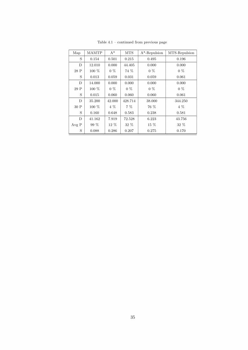
Table 4.1 – continued from previous page
Map MAMTP A* MTS A*-Repulsion MTS-Repulsion
S 0.154 0.501 0.215 0.495 0.196
D 12.010 0.000 44.405 0.000 0.000
28 P 100 % 0 % 74 % 0 % 0 %
S 0.013 0.059 0.031 0.059 0.061
D 14.000 0.000 0.000 0.000 0.000
29 P 100 % 0 % 0 % 0 % 0 %
S 0.015 0.060 0.060 0.060 0.061
D 35.200 42.000 428.714 38.000 344.250
30 P 100 % 4 % 7 % 76 % 4 %
S 0.160 0.648 0.583 0.238 0.581
D 41.162 7.919 72.528 6.223 43.756
Avg P 99 % 12 % 32 % 15 % 32 %
S 0.088 0.286 0.207 0.275 0.170
35
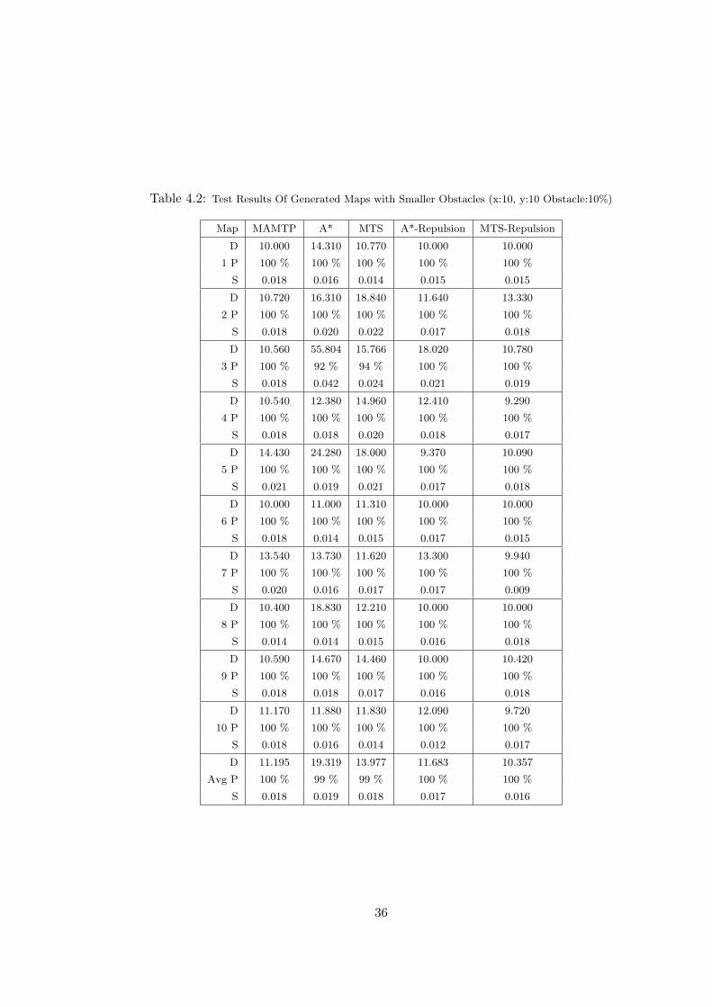
Table 4.2: Test Results Of Generated Maps with Smaller Obstacles (x:10, y:10 Obstacle:10%)
Map MAMTP A* MTS A*-Repulsion MTS-Repulsion
D 10.000 14.310 10.770 10.000 10.000
1 P 100 % 100 % 100 % 100 % 100 %
S 0.018 0.016 0.014 0.015 0.015
D 10.720 16.310 18.840 11.640 13.330
2 P 100 % 100 % 100 % 100 % 100 %
S 0.018 0.020 0.022 0.017 0.018
D 10.560 55.804 15.766 18.020 10.780
3 P 100 % 92 % 94 % 100 % 100 %
S 0.018 0.042 0.024 0.021 0.019
D 10.540 12.380 14.960 12.410 9.290
4 P 100 % 100 % 100 % 100 % 100 %
S 0.018 0.018 0.020 0.018 0.017
D 14.430 24.280 18.000 9.370 10.090
5 P 100 % 100 % 100 % 100 % 100 %
S 0.021 0.019 0.021 0.017 0.018
D 10.000 11.000 11.310 10.000 10.000
6 P 100 % 100 % 100 % 100 % 100 %
S 0.018 0.014 0.015 0.017 0.015
D 13.540 13.730 11.620 13.300 9.940
7 P 100 % 100 % 100 % 100 % 100 %
S 0.020 0.016 0.017 0.017 0.009
D 10.400 18.830 12.210 10.000 10.000
8 P 100 % 100 % 100 % 100 % 100 %
S 0.014 0.014 0.015 0.016 0.018
D 10.590 14.670 14.460 10.000 10.420
9 P 100 % 100 % 100 % 100 % 100 %
S 0.018 0.018 0.017 0.016 0.018
D 11.170 11.880 11.830 12.090 9.720
10 P 100 % 100 % 100 % 100 % 100 %
S 0.018 0.016 0.014 0.012 0.017
D 11.195 19.319 13.977 11.683 10.357
Avg P 100 % 99 % 99 % 100 % 100 %
S 0.018 0.019 0.018 0.017 0.016
36
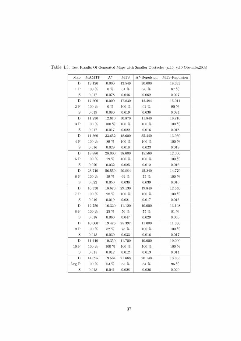
Table 4.3: Test Results Of Generated Maps with Smaller Obstacles (x:10, y:10 Obstacle:20%)
Map MAMTP A* MTS A*-Repulsion MTS-Repulsion
D 13.120 0.000 12.549 30.000 18.333
1 P 100 % 0 % 51 % 26 % 87 %
S 0.017 0.078 0.046 0.062 0.027
D 17.500 0.000 17.830 12.484 15.011
2 P 100 % 0 % 100 % 62 % 90 %
S 0.019 0.080 0.019 0.036 0.024
D 11.230 12.610 30.870 11.840 16.710
3 P 100 % 100 % 100 % 100 % 100 %
S 0.017 0.017 0.022 0.016 0.018
D 11.360 33.652 18.600 35.440 13.960
4 P 100 % 89 % 100 % 100 % 100 %
S 0.016 0.029 0.018 0.023 0.019
D 18.880 28.000 38.600 15.560 12.000
5 P 100 % 79 % 100 % 100 % 100 %
S 0.020 0.032 0.025 0.012 0.016
D 23.740 56.559 20.884 45.240 14.770
6 P 100 % 59 % 69 % 75 % 100 %
S 0.022 0.050 0.038 0.039 0.016
D 16.330 18.673 29.130 19.840 12.540
7 P 100 % 98 % 100 % 100 % 100 %
S 0.019 0.019 0.021 0.017 0.015
D 12.750 16.320 11.120 10.000 13.198
8 P 100 % 25 % 50 % 75 % 81 %
S 0.018 0.060 0.047 0.029 0.030
D 10.600 19.476 25.397 11.000 11.830
9 P 100 % 82 % 78 % 100 % 100 %
S 0.018 0.030 0.033 0.016 0.017
D 11.440 10.350 11.700 10.000 10.000
10 P 100 % 100 % 100 % 100 % 100 %
S 0.015 0.012 0.012 0.013 0.014
D 14.695 19.564 21.668 20.140 13.835
Avg P 100 % 63 % 85 % 84 % 96 %
S 0.018 0.041 0.028 0.026 0.020
37
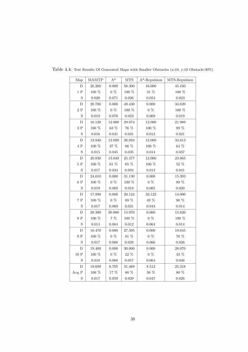
Table 4.4: Test Results Of Generated Maps with Smaller Obstacles (x:10, y:10 Obstacle:30%)
Map MAMTP A* MTS A*-Repulsion MTS-Repulsion
D 26.260 0.000 58.300 16.000 45.160
1 P 100 % 0 % 100 % 31 % 100 %
S 0.020 0.071 0.026 0.054 0.023
D 20.780 0.000 49.430 0.000 34.620
2 P 100 % 0 % 100 % 0 % 100 %
S 0.019 0.070 0.023 0.069 0.019
D 16.120 12.000 29.974 12.000 21.989
3 P 100 % 63 % 76 % 100 % 89 %
S 0.016 0.031 0.031 0.013 0.021
D 13.940 12.000 26.894 12.000 34.813
4 P 100 % 37 % 66 % 100 % 64 %
S 0.015 0.045 0.035 0.014 0.037
D 20.830 13.049 25.477 12.000 23.865
5 P 100 % 61 % 65 % 100 % 52 %
S 0.017 0.034 0.034 0.013 0.041
D 24.010 0.000 31.130 0.000 15.393
6 P 100 % 0 % 100 % 0 % 89 %
S 0.019 0.069 0.018 0.065 0.020
D 17.890 0.000 20.124 33.122 14.000
7 P 100 % 0 % 89 % 49 % 90 %
S 0.017 0.069 0.021 0.044 0.014
D 20.390 30.000 15.970 0.000 15.620
8 P 100 % 7 % 100 % 0 % 100 %
S 0.014 0.064 0.012 0.064 0.014
D 16.470 0.000 27.395 0.000 19.645
9 P 100 % 0 % 81 % 0 % 76 %
S 0.017 0.068 0.028 0.066 0.026
D 19.400 0.000 30.000 0.000 28.070
10 P 100 % 0 % 22 % 0 % 43 %
S 0.018 0.068 0.057 0.064 0.046
D 19.609 6.705 31.469 8.512 25.318
Avg P 100 % 17 % 80 % 38 % 80 %
S 0.017 0.059 0.029 0.047 0.026
38
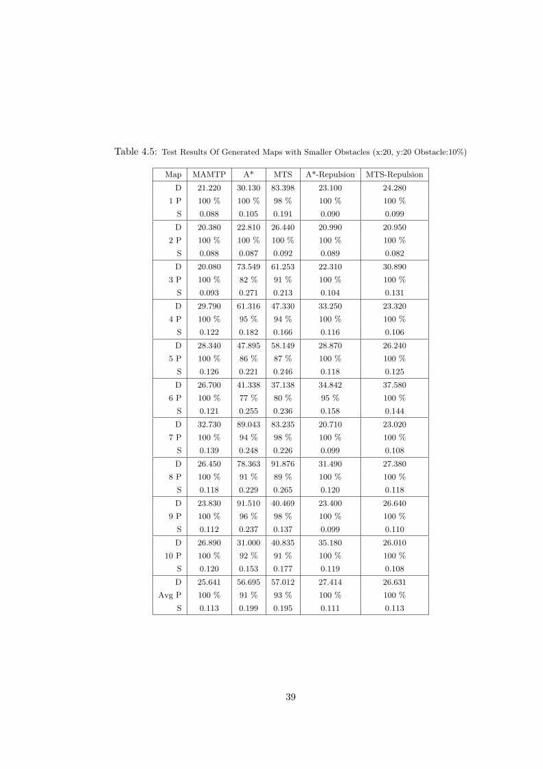
Table 4.5: Test Results Of Generated Maps with Smaller Obstacles (x:20, y:20 Obstacle:10%)
Map MAMTP A* MTS A*-Repulsion MTS-Repulsion
D 21.220 30.130 83.398 23.100 24.280
1 P 100 % 100 % 98 % 100 % 100 %
S 0.088 0.105 0.191 0.090 0.099
D 20.380 22.810 26.440 20.990 20.950
2 P 100 % 100 % 100 % 100 % 100 %
S 0.088 0.087 0.092 0.089 0.082
D 20.080 73.549 61.253 22.310 30.890
3 P 100 % 82 % 91 % 100 % 100 %
S 0.093 0.271 0.213 0.104 0.131
D 29.790 61.316 47.330 33.250 23.320
4 P 100 % 95 % 94 % 100 % 100 %
S 0.122 0.182 0.166 0.116 0.106
D 28.340 47.895 58.149 28.870 26.240
5 P 100 % 86 % 87 % 100 % 100 %
S 0.126 0.221 0.246 0.118 0.125
D 26.700 41.338 37.138 34.842 37.580
6 P 100 % 77 % 80 % 95 % 100 %
S 0.121 0.255 0.236 0.158 0.144
D 32.730 89.043 83.235 20.710 23.020
7 P 100 % 94 % 98 % 100 % 100 %
S 0.139 0.248 0.226 0.099 0.108
D 26.450 78.363 91.876 31.490 27.380
8 P 100 % 91 % 89 % 100 % 100 %
S 0.118 0.229 0.265 0.120 0.118
D 23.830 91.510 40.469 23.400 26.640
9 P 100 % 96 % 98 % 100 % 100 %
S 0.112 0.237 0.137 0.099 0.110
D 26.890 31.000 40.835 35.180 26.010
10 P 100 % 92 % 91 % 100 % 100 %
S 0.120 0.153 0.177 0.119 0.108
D 25.641 56.695 57.012 27.414 26.631
Avg P 100 % 91 % 93 % 100 % 100 %
S 0.113 0.199 0.195 0.111 0.113
39
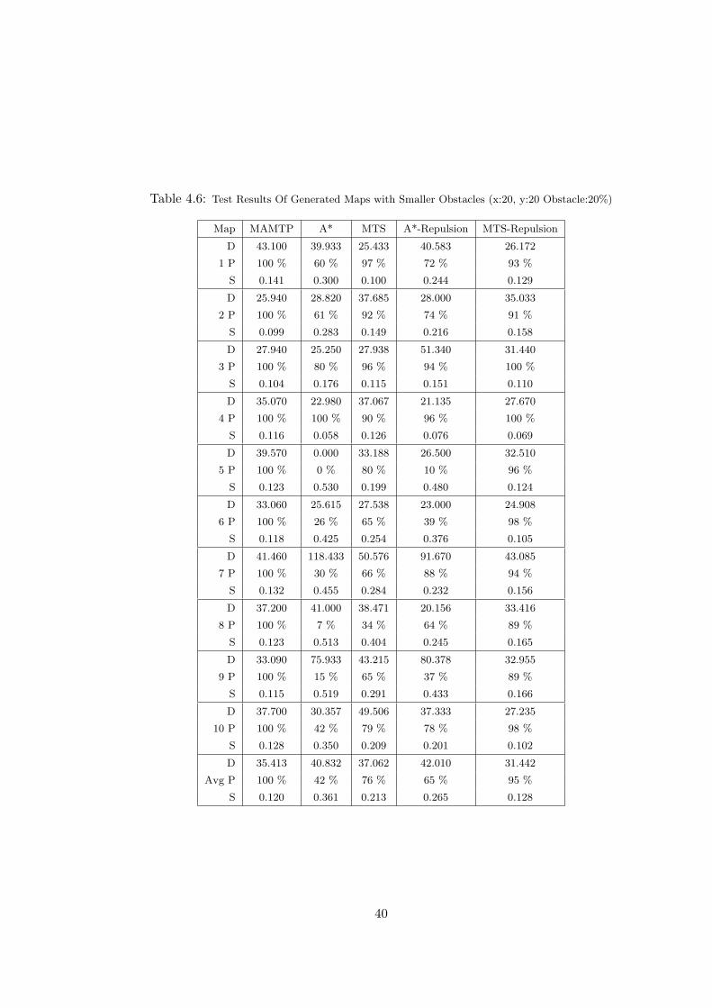
Table 4.6: Test Results Of Generated Maps with Smaller Obstacles (x:20, y:20 Obstacle:20%)
Map MAMTP A* MTS A*-Repulsion MTS-Repulsion
D 43.100 39.933 25.433 40.583 26.172
1 P 100 % 60 % 97 % 72 % 93 %
S 0.141 0.300 0.100 0.244 0.129
D 25.940 28.820 37.685 28.000 35.033
2 P 100 % 61 % 92 % 74 % 91 %
S 0.099 0.283 0.149 0.216 0.158
D 27.940 25.250 27.938 51.340 31.440
3 P 100 % 80 % 96 % 94 % 100 %
S 0.104 0.176 0.115 0.151 0.110
D 35.070 22.980 37.067 21.135 27.670
4 P 100 % 100 % 90 % 96 % 100 %
S 0.116 0.058 0.126 0.076 0.069
D 39.570 0.000 33.188 26.500 32.510
5 P 100 % 0 % 80 % 10 % 96 %
S 0.123 0.530 0.199 0.480 0.124
D 33.060 25.615 27.538 23.000 24.908
6 P 100 % 26 % 65 % 39 % 98 %
S 0.118 0.425 0.254 0.376 0.105
D 41.460 118.433 50.576 91.670 43.085
7 P 100 % 30 % 66 % 88 % 94 %
S 0.132 0.455 0.284 0.232 0.156
D 37.200 41.000 38.471 20.156 33.416
8 P 100 % 7 % 34 % 64 % 89 %
S 0.123 0.513 0.404 0.245 0.165
D 33.090 75.933 43.215 80.378 32.955
9 P 100 % 15 % 65 % 37 % 89 %
S 0.115 0.519 0.291 0.433 0.166
D 37.700 30.357 49.506 37.333 27.235
10 P 100 % 42 % 79 % 78 % 98 %
S 0.128 0.350 0.209 0.201 0.102
D 35.413 40.832 37.062 42.010 31.442
Avg P 100 % 42 % 76 % 65 % 95 %
S 0.120 0.361 0.213 0.265 0.128
40
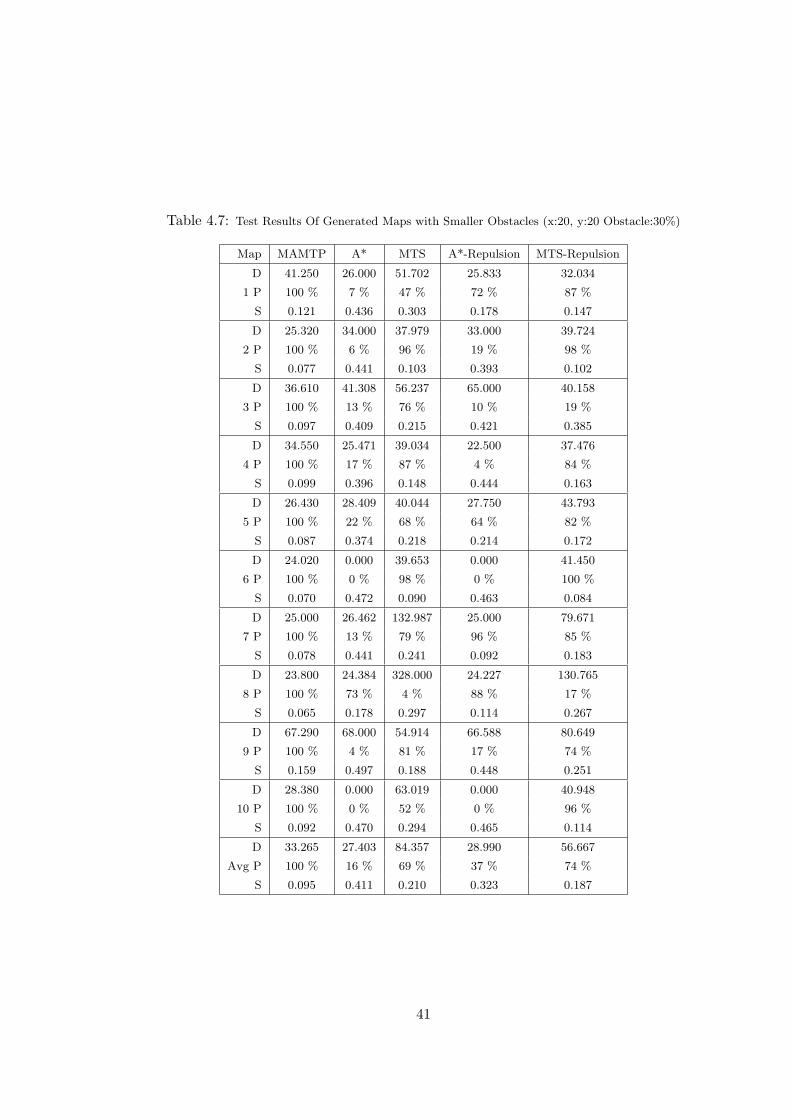
Table 4.7: Test Results Of Generated Maps with Smaller Obstacles (x:20, y:20 Obstacle:30%)
Map MAMTP A* MTS A*-Repulsion MTS-Repulsion
D 41.250 26.000 51.702 25.833 32.034
1 P 100 % 7 % 47 % 72 % 87 %
S 0.121 0.436 0.303 0.178 0.147
D 25.320 34.000 37.979 33.000 39.724
2 P 100 % 6 % 96 % 19 % 98 %
S 0.077 0.441 0.103 0.393 0.102
D 36.610 41.308 56.237 65.000 40.158
3 P 100 % 13 % 76 % 10 % 19 %
S 0.097 0.409 0.215 0.421 0.385
D 34.550 25.471 39.034 22.500 37.476
4 P 100 % 17 % 87 % 4 % 84 %
S 0.099 0.396 0.148 0.444 0.163
D 26.430 28.409 40.044 27.750 43.793
5 P 100 % 22 % 68 % 64 % 82 %
S 0.087 0.374 0.218 0.214 0.172
D 24.020 0.000 39.653 0.000 41.450
6 P 100 % 0 % 98 % 0 % 100 %
S 0.070 0.472 0.090 0.463 0.084
D 25.000 26.462 132.987 25.000 79.671
7 P 100 % 13 % 79 % 96 % 85 %
S 0.078 0.441 0.241 0.092 0.183
D 23.800 24.384 328.000 24.227 130.765
8 P 100 % 73 % 4 % 88 % 17 %
S 0.065 0.178 0.297 0.114 0.267
D 67.290 68.000 54.914 66.588 80.649
9 P 100 % 4 % 81 % 17 % 74 %
S 0.159 0.497 0.188 0.448 0.251
D 28.380 0.000 63.019 0.000 40.948
10 P 100 % 0 % 52 % 0 % 96 %
S 0.092 0.470 0.294 0.465 0.114
D 33.265 27.403 84.357 28.990 56.667
Avg P 100 % 16 % 69 % 37 % 74 %
S 0.095 0.411 0.210 0.323 0.187
41
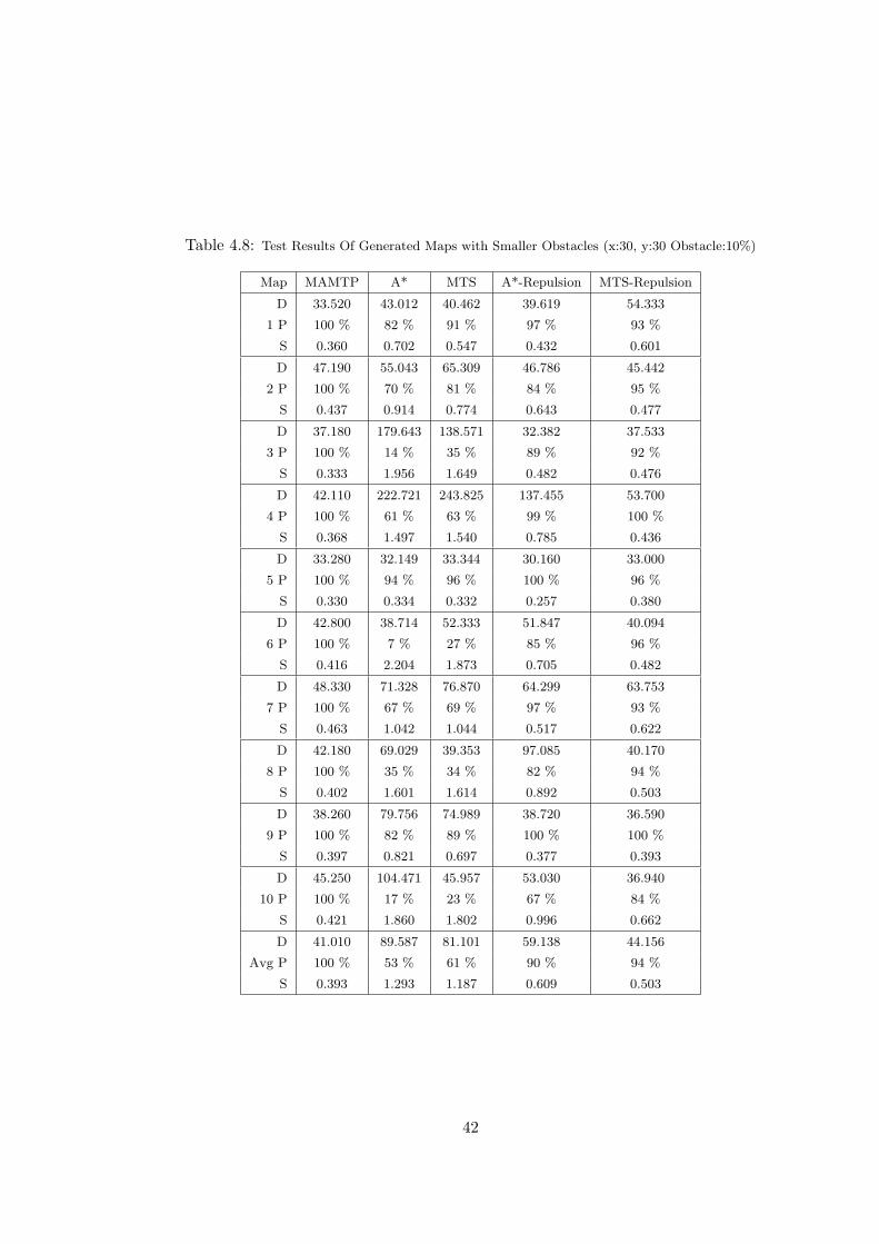
Table 4.8: Test Results Of Generated Maps with Smaller Obstacles (x:30, y:30 Obstacle:10%)
Map MAMTP A* MTS A*-Repulsion MTS-Repulsion
D 33.520 43.012 40.462 39.619 54.333
1 P 100 % 82 % 91 % 97 % 93 %
S 0.360 0.702 0.547 0.432 0.601
D 47.190 55.043 65.309 46.786 45.442
2 P 100 % 70 % 81 % 84 % 95 %
S 0.437 0.914 0.774 0.643 0.477
D 37.180 179.643 138.571 32.382 37.533
3 P 100 % 14 % 35 % 89 % 92 %
S 0.333 1.956 1.649 0.482 0.476
D 42.110 222.721 243.825 137.455 53.700
4 P 100 % 61 % 63 % 99 % 100 %
S 0.368 1.497 1.540 0.785 0.436
D 33.280 32.149 33.344 30.160 33.000
5 P 100 % 94 % 96 % 100 % 96 %
S 0.330 0.334 0.332 0.257 0.380
D 42.800 38.714 52.333 51.847 40.094
6 P 100 % 7 % 27 % 85 % 96 %
S 0.416 2.204 1.873 0.705 0.482
D 48.330 71.328 76.870 64.299 63.753
7 P 100 % 67 % 69 % 97 % 93 %
S 0.463 1.042 1.044 0.517 0.622
D 42.180 69.029 39.353 97.085 40.170
8 P 100 % 35 % 34 % 82 % 94 %
S 0.402 1.601 1.614 0.892 0.503
D 38.260 79.756 74.989 38.720 36.590
9 P 100 % 82 % 89 % 100 % 100 %
S 0.397 0.821 0.697 0.377 0.393
D 45.250 104.471 45.957 53.030 36.940
10 P 100 % 17 % 23 % 67 % 84 %
S 0.421 1.860 1.802 0.996 0.662
D 41.010 89.587 81.101 59.138 44.156
Avg P 100 % 53 % 61 % 90 % 94 %
S 0.393 1.293 1.187 0.609 0.503
42
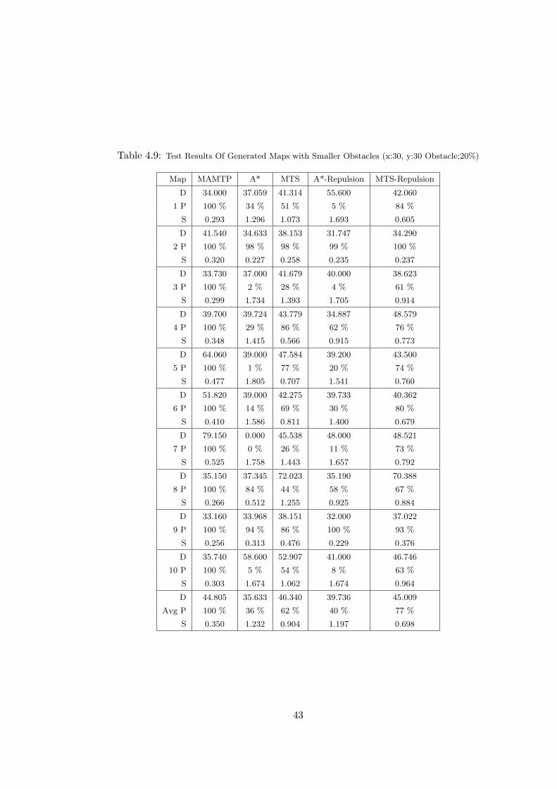
Table 4.9: Test Results Of Generated Maps with Smaller Obstacles (x:30, y:30 Obstacle:20%)
Map MAMTP A* MTS A*-Repulsion MTS-Repulsion
D 34.000 37.059 41.314 55.600 42.060
1 P 100 % 34 % 51 % 5 % 84 %
S 0.293 1.296 1.073 1.693 0.605
D 41.540 34.633 38.153 31.747 34.290
2 P 100 % 98 % 98 % 99 % 100 %
S 0.320 0.227 0.258 0.235 0.237
D 33.730 37.000 41.679 40.000 38.623
3 P 100 % 2 % 28 % 4 % 61 %
S 0.299 1.734 1.393 1.705 0.914
D 39.700 39.724 43.779 34.887 48.579
4 P 100 % 29 % 86 % 62 % 76 %
S 0.348 1.415 0.566 0.915 0.773
D 64.060 39.000 47.584 39.200 43.500
5 P 100 % 1 % 77 % 20 % 74 %
S 0.477 1.805 0.707 1.541 0.760
D 51.820 39.000 42.275 39.733 40.362
6 P 100 % 14 % 69 % 30 % 80 %
S 0.410 1.586 0.811 1.400 0.679
D 79.150 0.000 45.538 48.000 48.521
7 P 100 % 0 % 26 % 11 % 73 %
S 0.525 1.758 1.443 1.657 0.792
D 35.150 37.345 72.023 35.190 70.388
8 P 100 % 84 % 44 % 58 % 67 %
S 0.266 0.512 1.255 0.925 0.884
D 33.160 33.968 38.151 32.000 37.022
9 P 100 % 94 % 86 % 100 % 93 %
S 0.256 0.313 0.476 0.229 0.376
D 35.740 58.600 52.907 41.000 46.746
10 P 100 % 5 % 54 % 8 % 63 %
S 0.303 1.674 1.062 1.674 0.964
D 44.805 35.633 46.340 39.736 45.009
Avg P 100 % 36 % 62 % 40 % 77 %
S 0.350 1.232 0.904 1.197 0.698
43
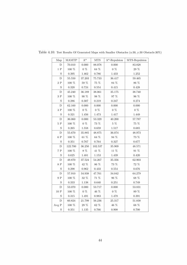
Table 4.10: Test Results Of Generated Maps with Smaller Obstacles (x:30, y:30 Obstacle:30%)
Map MAMTP A* MTS A*-Repulsion MTS-Repulsion
D 70.010 0.000 88.078 0.000 83.828
1 P 100 % 0 % 64 % 0 % 29 %
S 0.395 1.462 0.786 1.433 1.252
D 55.550 37.203 75.733 36.417 59.465
2 P 100 % 59 % 75 % 84 % 86 %
S 0.320 0.724 0.554 0.415 0.428
D 45.240 36.189 38.061 35.175 38.740
3 P 100 % 90 % 98 % 97 % 96 %
S 0.286 0.307 0.219 0.247 0.274
D 62.160 0.000 0.000 0.000 0.000
4 P 100 % 0 % 0 % 0 % 0 %
S 0.321 1.456 1.473 1.417 1.449
D 36.060 0.000 53.329 40.200 57.787
5 P 100 % 0 % 73 % 5 % 75 %
S 0.265 1.558 0.659 1.517 0.685
D 55.670 35.885 48.875 36.074 48.973
6 P 100 % 61 % 64 % 94 % 73 %
S 0.351 0.767 0.764 0.327 0.677
D 122.700 36.250 102.537 35.909 48.571
7 P 100 % 8 % 41 % 11 % 91 %
S 0.625 1.481 1.153 1.439 0.420
D 49.870 37.524 54.267 35.356 62.903
8 P 100 % 42 % 86 % 73 % 72 %
S 0.298 0.962 0.433 0.554 0.676
D 57.910 34.938 47.761 34.042 64.279
9 P 100 % 32 % 71 % 96 % 68 %
S 0.333 1.138 0.640 0.251 0.749
D 53.070 0.000 53.717 0.000 53.831
10 P 100 % 0 % 46 % 0 % 89 %
S 0.315 1.491 0.983 1.478 0.391
D 60.824 21.799 56.236 25.317 51.838
Avg P 100 % 29 % 62 % 46 % 68 %
S 0.351 1.135 0.766 0.908 0.700
44
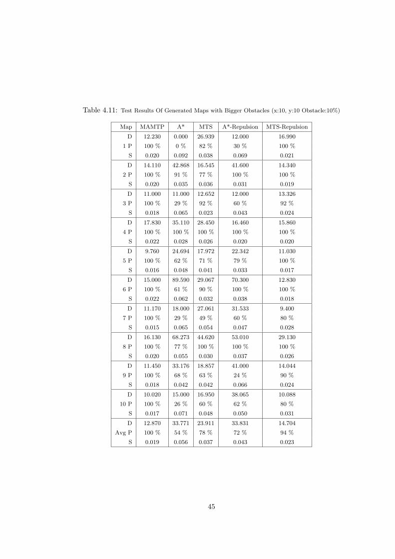
Table 4.11: Test Results Of Generated Maps with Bigger Obstacles (x:10, y:10 Obstacle:10%)
Map MAMTP A* MTS A*-Repulsion MTS-Repulsion
D 12.230 0.000 26.939 12.000 16.990
1 P 100 % 0 % 82 % 30 % 100 %
S 0.020 0.092 0.038 0.069 0.021
D 14.110 42.868 16.545 41.600 14.340
2 P 100 % 91 % 77 % 100 % 100 %
S 0.020 0.035 0.036 0.031 0.019
D 11.000 11.000 12.652 12.000 13.326
3 P 100 % 29 % 92 % 60 % 92 %
S 0.018 0.065 0.023 0.043 0.024
D 17.830 35.110 28.450 16.460 15.860
4 P 100 % 100 % 100 % 100 % 100 %
S 0.022 0.028 0.026 0.020 0.020
D 9.760 24.694 17.972 22.342 11.030
5 P 100 % 62 % 71 % 79 % 100 %
S 0.016 0.048 0.041 0.033 0.017
D 15.000 89.590 29.067 70.300 12.830
6 P 100 % 61 % 90 % 100 % 100 %
S 0.022 0.062 0.032 0.038 0.018
D 11.170 18.000 27.061 31.533 9.400
7 P 100 % 29 % 49 % 60 % 80 %
S 0.015 0.065 0.054 0.047 0.028
D 16.130 68.273 44.620 53.010 29.130
8 P 100 % 77 % 100 % 100 % 100 %
S 0.020 0.055 0.030 0.037 0.026
D 11.450 33.176 18.857 41.000 14.044
9 P 100 % 68 % 63 % 24 % 90 %
S 0.018 0.042 0.042 0.066 0.024
D 10.020 15.000 16.950 38.065 10.088
10 P 100 % 26 % 60 % 62 % 80 %
S 0.017 0.071 0.048 0.050 0.031
D 12.870 33.771 23.911 33.831 14.704
Avg P 100 % 54 % 78 % 72 % 94 %
S 0.019 0.056 0.037 0.043 0.023
45

Table 4.12: Test Results Of Generated Maps with Bigger Obstacles (x:10, y:10 Obstacle:20%)
Map MAMTP A* MTS A*-Repulsion MTS-Repulsion
D 15.960 0.000 40.438 54.588 18.790
1 P 100 % 0 % 73 % 51 % 100 %
S 0.020 0.078 0.043 0.053 0.020
D 12.000 14.420 57.060 13.000 27.120
2 P 100 % 100 % 100 % 90 % 100 %
S 0.018 0.017 0.029 0.023 0.020
D 11.420 0.000 79.877 0.000 57.025
3 P 100 % 0 % 81 % 0 % 80 %
S 0.018 0.076 0.040 0.075 0.045
D 12.000 0.000 39.146 0.000 25.000
4 P 100 % 0 % 89 % 0 % 27 %
S 0.017 0.079 0.029 0.079 0.062
D 13.000 0.000 61.160 0.000 35.530
5 P 100 % 0 % 100 % 0 % 100 %
S 0.019 0.080 0.036 0.079 0.027
D 14.000 65.632 39.917 32.000 39.600
6 P 100 % 57 % 72 % 88 % 100 %
S 0.018 0.053 0.039 0.027 0.025
D 13.000 0.000 34.520 0.000 23.420
7 P 100 % 0 % 100 % 0 % 100 %
S 0.017 0.077 0.021 0.077 0.020
D 11.520 11.742 14.020 11.350 12.680
8 P 100 % 89 % 100 % 100 % 100 %
S 0.017 0.020 0.013 0.012 0.013
D 20.880 0.000 38.253 0.000 20.610
9 P 100 % 0 % 75 % 0 % 100 %
S 0.020 0.078 0.037 0.077 0.019
D 12.770 11.000 15.083 22.022 11.620
10 P 100 % 11 % 72 % 93 % 100 %
S 0.017 0.073 0.034 0.023 0.015
D 13.655 10.279 41.947 13.296 27.140
Avg P 100 % 26 % 86 % 42 % 91 %
S 0.018 0.063 0.032 0.053 0.027
46
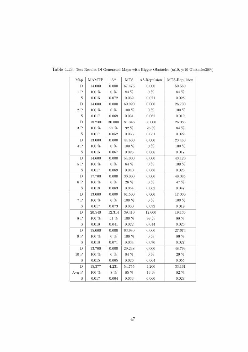
Table 4.13: Test Results Of Generated Maps with Bigger Obstacles (x:10, y:10 Obstacle:30%)
Map MAMTP A* MTS A*-Repulsion MTS-Repulsion
D 14.000 0.000 67.476 0.000 50.560
1 P 100 % 0 % 84 % 0 % 84 %
S 0.015 0.072 0.032 0.071 0.028
D 14.000 0.000 69.920 0.000 26.700
2 P 100 % 0 % 100 % 0 % 100 %
S 0.017 0.069 0.031 0.067 0.019
D 18.230 30.000 81.348 30.000 26.083
3 P 100 % 27 % 92 % 28 % 84 %
S 0.017 0.052 0.033 0.051 0.022
D 13.000 0.000 44.680 0.000 23.460
4 P 100 % 0 % 100 % 0 % 100 %
S 0.015 0.067 0.025 0.066 0.017
D 14.600 0.000 54.000 0.000 43.120
5 P 100 % 0 % 64 % 0 % 100 %
S 0.017 0.069 0.040 0.066 0.023
D 17.700 0.000 36.000 0.000 49.085
6 P 100 % 0 % 26 % 0 % 47 %
S 0.018 0.063 0.054 0.062 0.047
D 13.000 0.000 61.500 0.000 17.000
7 P 100 % 0 % 100 % 0 % 100 %
S 0.017 0.073 0.030 0.072 0.019
D 20.540 12.314 39.410 12.000 19.136
8 P 100 % 51 % 100 % 98 % 88 %
S 0.018 0.041 0.022 0.014 0.023
D 15.000 0.000 63.980 0.000 27.674
9 P 100 % 0 % 100 % 0 % 86 %
S 0.018 0.071 0.034 0.070 0.027
D 13.700 0.000 29.238 0.000 48.793
10 P 100 % 0 % 84 % 0 % 29 %
S 0.015 0.065 0.026 0.064 0.055
D 15.377 4.231 54.755 4.200 33.161
Avg P 100 % 8 % 85 % 13 % 82 %
S 0.017 0.064 0.033 0.060 0.028
47
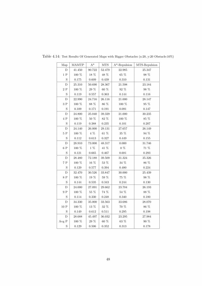
Table 4.14: Test Results Of Generated Maps with Bigger Obstacles (x:20, y:20 Obstacle:10%)
Map MAMTP A* MTS A*-Repulsion MTS-Repulsion
D 41.450 90.722 52.479 22.985 25.347
1 P 100 % 18 % 48 % 65 % 98 %
S 0.175 0.609 0.439 0.310 0.131
D 25.310 50.690 28.367 21.598 23.184
2 P 100 % 29 % 60 % 92 % 98 %
S 0.119 0.557 0.363 0.144 0.116
D 22.990 24.716 26.116 21.000 28.147
3 P 100 % 88 % 86 % 100 % 95 %
S 0.109 0.171 0.191 0.091 0.147
D 24.800 25.040 39.329 21.000 30.235
4 P 100 % 50 % 82 % 100 % 85 %
S 0.119 0.388 0.235 0.101 0.207
D 24.140 26.000 29.131 27.657 26.149
5 P 100 % 4 % 61 % 35 % 94 %
S 0.112 0.613 0.327 0.449 0.155
D 28.910 73.000 48.317 0.000 31.746
6 P 100 % 1 % 41 % 0 % 71 %
S 0.121 0.665 0.467 0.681 0.293
D 28.480 72.188 39.509 31.324 35.326
7 P 100 % 16 % 53 % 34 % 86 %
S 0.129 0.577 0.394 0.480 0.224
D 32.470 30.526 33.847 30.000 25.439
8 P 100 % 19 % 59 % 75 % 98 %
S 0.144 0.535 0.343 0.244 0.130
D 24.000 27.091 29.662 23.704 26.193
9 P 100 % 55 % 74 % 54 % 88 %
S 0.114 0.330 0.248 0.340 0.180
D 34.330 35.000 33.563 33.686 28.070
10 P 100 % 13 % 32 % 70 % 86 %
S 0.149 0.612 0.511 0.295 0.198
D 28.688 45.497 36.032 23.295 27.984
Avg P 100 % 29 % 60 % 63 % 90 %
S 0.129 0.506 0.352 0.313 0.178
48
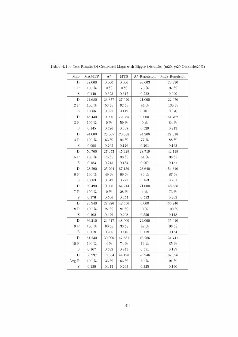
Table 4.15: Test Results Of Generated Maps with Bigger Obstacles (x:20, y:20 Obstacle:20%)
Map MAMTP A* MTS A*-Repulsion MTS-Repulsion
D 38.000 0.000 0.000 20.603 23.330
1 P 100 % 0 % 0 % 73 % 97 %
S 0.140 0.623 0.317 0.222 0.099
D 24.680 23.377 27.620 21.000 22.670
2 P 100 % 53 % 92 % 94 % 100 %
S 0.086 0.327 0.119 0.101 0.070
D 43.430 0.000 72.085 0.000 51.762
3 P 100 % 0 % 59 % 0 % 84 %
S 0.145 0.526 0.338 0.529 0.213
D 24.000 25.365 26.638 24.208 27.818
4 P 100 % 63 % 94 % 77 % 88 %
S 0.098 0.265 0.126 0.201 0.163
D 56.700 27.053 45.429 28.719 42.719
5 P 100 % 75 % 98 % 64 % 96 %
S 0.183 0.215 0.134 0.267 0.151
D 23.290 25.204 67.159 23.640 54.310
6 P 100 % 49 % 69 % 86 % 87 %
S 0.083 0.342 0.273 0.153 0.201
D 59.490 0.000 64.214 71.000 48.658
7 P 100 % 0 % 28 % 4 % 73 %
S 0.176 0.566 0.454 0.553 0.263
D 25.940 27.926 42.556 0.000 35.240
8 P 100 % 27 % 81 % 0 % 100 %
S 0.102 0.426 0.208 0.556 0.118
D 36.210 24.617 48.000 24.000 35.010
9 P 100 % 60 % 33 % 92 % 96 %
S 0.118 0.266 0.416 0.118 0.134
D 51.230 30.000 47.581 49.286 31.741
10 P 100 % 4 % 74 % 14 % 85 %
S 0.167 0.582 0.243 0.551 0.189
D 38.297 18.354 44.128 26.246 37.326
Avg P 100 % 33 % 63 % 50 % 91 %
S 0.130 0.414 0.263 0.325 0.160
49

Table 4.16: Test Results Of Generated Maps with Bigger Obstacles (x:20, y:20 Obstacle:30%)
Map MAMTP A* MTS A*-Repulsion MTS-Repulsion
D 61.980 0.000 0.000 0.000 0.000
1 P 100 % 0 % 0 % 0 % 0 %
S 0.171 0.525 0.529 0.518 0.528
D 34.130 0.000 69.745 0.000 35.510
2 P 100 % 0 % 47 % 0 % 96 %
S 0.108 0.494 0.338 0.502 0.120
D 30.000 32.724 0.000 30.802 367.188
3 P 100 % 29 % 0 % 96 % 32 %
S 0.086 0.405 0.326 0.109 0.321
D 43.030 26.000 102.116 24.533 60.510
4 P 100 % 10 % 86 % 45 % 96 %
S 0.115 0.473 0.237 0.312 0.154
D 30.370 0.000 173.667 0.000 106.297
5 P 100 % 0 % 9 % 0 % 74 %
S 0.098 0.479 0.277 0.477 0.217
D 30.700 53.000 192.936 57.000 116.878
6 P 100 % 4 % 78 % 3 % 98 %
S 0.105 0.505 0.259 0.511 0.177
D 31.960 28.368 144.754 27.896 101.570
7 P 100 % 57 % 65 % 96 % 86 %
S 0.104 0.275 0.326 0.101 0.223
D 26.220 0.000 61.721 0.000 66.820
8 P 100 % 0 % 86 % 0 % 100 %
S 0.084 0.471 0.170 0.465 0.136
D 30.450 0.000 294.490 0.000 161.783
9 P 100 % 0 % 51 % 0 % 69 %
S 0.103 0.516 0.472 0.517 0.348
D 51.340 0.000 93.569 0.000 73.419
10 P 100 % 0 % 72 % 0 % 86 %
S 0.151 0.541 0.290 0.530 0.223
D 37.018 14.009 113.300 14.023 108.997
Avg P 100 % 10 % 49 % 24 % 74 %
S 0.112 0.468 0.322 0.404 0.245
50
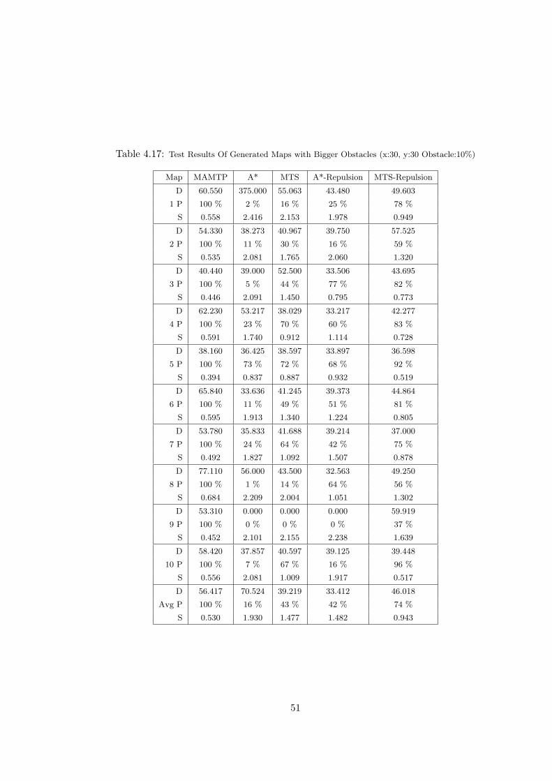
Table 4.17: Test Results Of Generated Maps with Bigger Obstacles (x:30, y:30 Obstacle:10%)
Map MAMTP A* MTS A*-Repulsion MTS-Repulsion
D 60.550 375.000 55.063 43.480 49.603
1 P 100 % 2 % 16 % 25 % 78 %
S 0.558 2.416 2.153 1.978 0.949
D 54.330 38.273 40.967 39.750 57.525
2 P 100 % 11 % 30 % 16 % 59 %
S 0.535 2.081 1.765 2.060 1.320
D 40.440 39.000 52.500 33.506 43.695
3 P 100 % 5 % 44 % 77 % 82 %
S 0.446 2.091 1.450 0.795 0.773
D 62.230 53.217 38.029 33.217 42.277
4 P 100 % 23 % 70 % 60 % 83 %
S 0.591 1.740 0.912 1.114 0.728
D 38.160 36.425 38.597 33.897 36.598
5 P 100 % 73 % 72 % 68 % 92 %
S 0.394 0.837 0.887 0.932 0.519
D 65.840 33.636 41.245 39.373 44.864
6 P 100 % 11 % 49 % 51 % 81 %
S 0.595 1.913 1.340 1.224 0.805
D 53.780 35.833 41.688 39.214 37.000
7 P 100 % 24 % 64 % 42 % 75 %
S 0.492 1.827 1.092 1.507 0.878
D 77.110 56.000 43.500 32.563 49.250
8 P 100 % 1 % 14 % 64 % 56 %
S 0.684 2.209 2.004 1.051 1.302
D 53.310 0.000 0.000 0.000 59.919
9 P 100 % 0 % 0 % 0 % 37 %
S 0.452 2.101 2.155 2.238 1.639
D 58.420 37.857 40.597 39.125 39.448
10 P 100 % 7 % 67 % 16 % 96 %
S 0.556 2.081 1.009 1.917 0.517
D 56.417 70.524 39.219 33.412 46.018
Avg P 100 % 16 % 43 % 42 % 74 %
S 0.530 1.930 1.477 1.482 0.943
51
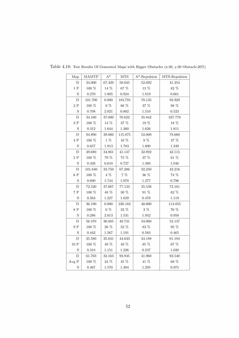
Table 4.18: Test Results Of Generated Maps with Bigger Obstacles (x:30, y:30 Obstacle:20%)
Map MAMTP A* MTS A*-Repulsion MTS-Repulsion
D 34.000 67.429 58.045 52.692 41.354
1 P 100 % 14 % 67 % 13 % 82 %
S 0.270 1.805 0.924 1.819 0.661
D 101.700 0.000 183.791 70.135 92.929
2 P 100 % 0 % 86 % 37 % 98 %
S 0.708 2.021 0.802 1.510 0.523
D 34.160 37.000 76.622 35.842 327.778
3 P 100 % 14 % 37 % 19 % 18 %
S 0.312 1.644 1.360 1.626 1.811
D 94.890 39.000 115.875 52.000 78.660
4 P 100 % 1 % 16 % 9 % 47 %
S 0.657 1.913 1.783 1.800 1.349
D 49.680 34.861 41.147 32.892 42.115
5 P 100 % 79 % 75 % 37 % 61 %
S 0.426 0.610 0.727 1.380 1.046
D 101.840 33.750 67.286 32.250 42.216
6 P 100 % 4 % 7 % 36 % 74 %
S 0.690 1.744 1.870 1.277 0.796
D 72.520 37.667 77.133 35.538 72.161
7 P 100 % 48 % 30 % 91 % 62 %
S 0.564 1.227 1.629 0.476 1.119
D 36.190 0.000 226.182 40.000 114.855
8 P 100 % 0 % 33 % 3 % 76 %
S 0.286 2.013 1.531 1.942 0.958
D 56.470 36.885 48.731 34.060 52.137
9 P 100 % 26 % 52 % 83 % 95 %
S 0.442 1.567 1.191 0.583 0.465
D 35.580 35.041 44.633 34.188 61.194
10 P 100 % 49 % 49 % 85 % 67 %
S 0.318 1.151 1.226 0.537 1.020
D 61.703 32.163 93.945 41.960 92.540
Avg P 100 % 24 % 45 % 41 % 68 %
S 0.467 1.570 1.304 1.295 0.975
52
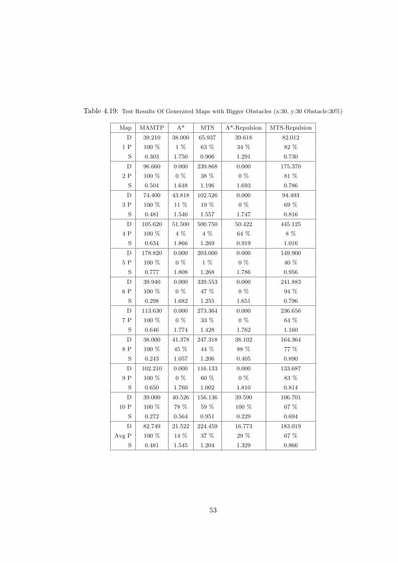
Table 4.19: Test Results Of Generated Maps with Bigger Obstacles (x:30, y:30 Obstacle:30%)
Map MAMTP A* MTS A*-Repulsion MTS-Repulsion
D 39.210 38.000 65.937 39.618 82.012
1 P 100 % 1 % 63 % 34 % 82 %
S 0.303 1.750 0.906 1.291 0.730
D 96.660 0.000 239.868 0.000 175.370
2 P 100 % 0 % 38 % 0 % 81 %
S 0.504 1.648 1.196 1.693 0.786
D 74.400 43.818 102.526 0.000 94.493
3 P 100 % 11 % 19 % 0 % 69 %
S 0.481 1.540 1.557 1.747 0.816
D 105.620 51.500 500.750 50.422 445.125
4 P 100 % 4 % 4 % 64 % 8 %
S 0.634 1.866 1.269 0.919 1.016
D 178.820 0.000 203.000 0.000 149.900
5 P 100 % 0 % 1 % 0 % 40 %
S 0.777 1.808 1.268 1.786 0.956
D 39.940 0.000 339.553 0.000 241.883
6 P 100 % 0 % 47 % 0 % 94 %
S 0.298 1.682 1.255 1.651 0.796
D 113.630 0.000 273.364 0.000 236.656
7 P 100 % 0 % 33 % 0 % 64 %
S 0.646 1.774 1.428 1.762 1.160
D 38.000 41.378 247.318 38.102 164.364
8 P 100 % 45 % 44 % 88 % 77 %
S 0.243 1.057 1.206 0.405 0.890
D 102.210 0.000 116.133 0.000 133.687
9 P 100 % 0 % 60 % 0 % 83 %
S 0.650 1.760 1.002 1.810 0.814
D 39.000 40.526 156.136 39.590 106.701
10 P 100 % 78 % 59 % 100 % 67 %
S 0.272 0.564 0.951 0.229 0.694
D 82.749 21.522 224.459 16.773 183.019
Avg P 100 % 14 % 37 % 29 % 67 %
S 0.481 1.545 1.204 1.329 0.866
53
Chapter 5
Conclusion and Future Work
5.1 Conclusion
As shown in the test results, and mentioned before, there was no algorithm specifically
designed for the multi-agent moving target search environment, but there are a lot of
possibilities. The results show us there is a fertile research field for multi-agent envi-
ronment and moving target search problem. A few new algorithms for our problem,
that can be used for comparison with our algorithm, are expected to be available
soon in the near future.
When there exists more algorithms that can be applied to this problem, we will
be able to make more meaningful comparisons.
Although other algorithms spend less time at each turn, the paths computed are
not good enough. Our algorithm can plan the alternative paths, which is demon-
strated in Figure 1.1, and therefore our algorithm is faster than its counterparts in
terms of the overall pursuit time.
A successful target algorithm is developed. It can elude capture from the known
algorithms of today (all single agent search algorithms, and multi-agent moving target
search), except the one agent algorithm, which we developed. Both of our algorithms
give good results, but not as good as human controlled agents or targets.
Human controlled targets may elude the capture, or postpone it as much as they
could, while the target algorithm fails under the same circumstances. With the same
conditions human controlled agents would capture the human controlled target, and
this shows us the necessity of improvement for both of our algorithms. They are not
optimum in any sense.
54
Moving targets, and multi-agent coordination fields offer endless possibilities of
new ideas.
5.2 Future Work
5.2.1 Future Work on The Environment Properties
To define a more realistic environment the assumptions can be relaxed:
• There may be multiple targets (the agents will need more time to choose a goal,
and all of the team members may not have the same goal in this definition)
• The diagonal moves have the same cost as other moves. Realistic costs for
moves can be tested.
• Simultaneous movement of agents can be implemented.
• Partially visible grid and dynamic grid environments can be handled. If our
algorithm is inserted into the pursuit part of MAMTS algorithm, the problem
will be solved. These properties will just make the average complexity of the
algorithm closer to the worst case complexity.
5.2.2 Future Work on The Target Algorithm
The target algorithm does not detect cycles, so instead of cycling around an obstacle,
it may prefer to get into a long dead end, calculating it will survive longer in that
dead end. If this property can be added to the algorithm, we may have a more
realistic target algorithm (with much more human like behavior)
Current target algorithm cannot evade the current agent algorithm, but a human
controlled target can evade the agents. It is obvious that our target cannot find the
optimum escape route.
An improvement of speed might be achieved by eliminating computation at every
turn, and aiming at the location which is computed during the last turn (similar to
the “commitment to goal” extension of MTS). This improvement will degrade the
evasion path quality, and therefore left as a future work.
Also commitment to goal extension might improve the path quality instead of
computation time. The new goal for the target can be recalculated each turn, but
55
the goal node computed in the last turn can be chosen only if it is still in the group
of best possibilities. If it is not one of the best solutions, then a new goal will be
selected. This method will not improve the computation time, but it will remove the
possible oscillation of the target, which is caused by the selection of different goals in
different directions in each turn, even though goal nodes in the same direction exists.
Therefore this method will improve the evasion path quality.
5.2.3 Future Work on The Agent Algorithm
Although the current agent algorithm is fast enough to be considered as real-time,
there are endless possibilities to speed it up. This is the primary objective of the
future works.
Possible ideas to speed up the algorithm’s time spent at each turn are as follows:
• The first idea would be to cache the calculated paths, and use it for some
time. This will reduce the time used at each turn dramatically. The paths
might get longer, so this idea has to be improved. If we can find a simple
condition that may tell us the necessity of the recomputation of the path, then
this improvement would not end up with longer pursuit paths.
• Using state abstraction in maps would decrease the complexity arguments of
our algorithm [10] [11]. If you don’t have an abstraction of the map already
(which is generally the case) calculating the state abstraction will have some
overhead, so it should be analyzed if the overhead is worth the time it costs.
Even simple abstractions will speed up our algorithm, so it is not critical to
calculate good abstractions.
Another improvement possibility is to achieve shorter paths:
• The current algorithm is not performing optimally. Human controlled agents
capture the targets faster than our algorithm. Even though it means more
calculations and more time, we can still improve our algorithm to obtain shorter
paths by close coordination of the agents.
• These agents may not be able to catch some human controlled targets, while
human controlled agents can. So we do not claim that our algorithm plans the
optimum path to capture a moving target. The coordination of the agents may
be improved.
56
• In the current agent algorithm when we find another agent, which is closer
to the midpoint of the path in process, we search for another path. But the
other agent which is closer to the midpoint, may have already planned to guard
another path. Before we search for another path, there may be a simple check
to detect if that agent really guards the path that is in process.
57
References
[1] S. Russell and P. Norving. Artificial Intelligence: a modern approach. Prentice
Hall, 1995.
[2] N. J. Nilsson. Problem Solving Methods in Artificial Intelligence. McGraw-Hill,
New York, 1971.
[3] Sven Koenig and Maxim Likhachev. D*lite. In Eighteenth national conference
on Artificial intelligence, pages 476–483, Menlo Park, CA, USA, 2002. American
Association for Artificial Intelligence.
[4] Sven Koenig and Maxim Likhachev. Fast replanning for robot navigation in
unknown terrain. IEEE Transactions on Robotics, 21(3):354–363, 2005.
[5] Toru Ishida and Richard E. Korf. Moving target search. In Proceedings of the
International Joint Conference on Artificial Intelligence IJCAI, pages 204–211,
1991.
[6] Toru Ishida and Richard E. Korf. Moving-target search: A real-time search for
changing goals. IEEE Transactions on Pattern Analysis and Machine Intelli-
gence, 17(6):609–619, 1995.
[7] Ken-ichi Teranishi Yasuhiko Kitamura and Shoji Tatsumi. Organizational strate-
gies for multiagent real-time search. In ICMAS, pages 150–156, 1996.
[8] X. Wu M. Goldenberg, A. Kovarksy and J. Schaeffer. Multiple agents moving
target search. In Proceedings of the International Joint Conference on Artificial
Intelligence IJCAI, pages 1538–1538, 2003.
[9] Freeciv A free clone of the Famous Strategy Game Civilization.
http://www.freeciv.org, last date accessed: 2007, 8 January.
[10] Vadim Bulitko, Nathan Sturtevant, and Maryia Kazakevich. Speeding up learn-
ing in real-time search via automatic state abstraction. In Proceedings of the
58
International Joint Conference on Artificial Intelligence (IJCAI), Workshop on
Planning and Learning in A Priori Unknown or Dynamic Domains, pages 55 –
61, Edinburgh, UK, 2005.
[11] Vadim Bulitko and Nathan Sturtevant. State abstraction for real-time moving
target pursuit: A pilot study. In Proceedings of the National Conference on
Artificial Intelligence (AAAI), Workshop on Learning For Search, pages 72–79,
Boston, Massachusetts, 2006.
[12] Sviatoslav Braynov Ramachandra Kota and James Llinas. Multi-agent moving
target search in a hazy environment. In Integration of Knowledge Intensive
Multi-Agent Systems, pages 275– 278, 2003.
[13] Toru Ishida. Real-time search for autonomous agents and multiagent systems.
Autonomous Agents and Multi-Agent Systems, 1(2):139–167, 1998.
[14] Patrick Lester. A star tutorial for beginners.
http://www.policyalmanac.org/games/aStarTutorial.htm, last date accessed:
2007, 8 January.
[15] Richard E. Korf. Real-time heuristic search. Artif. Intell., 42(2-3):189–211, 1990.
[16] M. Yokoo and Y. Kitamura. Multiagent real-time a* with selection: Introducing
competition in cooperative search. International Conference on Multi-Agent
Systems (ICMAS-96), pages 409–416, 1996.
59