Embed Size (px)
Citation preview

1
Multi-year Long-term Load Forecast for Area
Distribution Feeders based on Selective Sequence
Learning
Ming Donga, Jian Shi
b ,Qingxin Shi
c,*
a: Dept. of Grid Reliability, Alberta Electric System Operator; T2P 0L4, AB, Canada
b: Dept. of Electrical and Computer Engineering, University of Houston; TX 77204-4005, USA
c: Dept. of Electrical Engineering and Computer Science, The University of Tennessee; TN 37996,
USA
*: Corresponding author email: [email protected]
Abstract - Area feeder long-term load forecast (LTLF) is one of the most critical forecasting tasks in electric
distribution utility companies. Cost effective system upgrades can only be planned out based on accurate
feeder LTLF results. However, the commonly used top-down and bottom-up LTLF methods fail to combine
area and feeder information and cannot effectively deal with component-level LTLF. The previous research
effort on hybrid approach that aims to combine top-down and bottom-up approaches is very limited. The
recent work only focuses on the forecast of the next one-year and uses a one-fit-all model for all area feeders.
In response, this paper proposes a novel selective sequence learning method that can convert a multi-year
LTLF problem to a multi-timestep sequence prediction problem. The model learns how to predict sequence
values as well as the best-performing sequential configuration for each feeder. In addition, unsupervised
learning is introduced to automatically group feeders based on load compositions ahead of learning to
further enhance the performance. The proposed method was tested on an urban distribution system in
Canada and compared with many conventional methods and the existing hybrid forecasting method. It
achieves the best forecasting accuracy measured by three metrics AMAPE, RMSE and R-squared. It also
proves the feasibility of applying sequence learning to multi-year component-level load forecast.
KEY WORDS: Long-term Load Forecast, Multi-timestep Sequence Prediction, Unsupervised learning

2
1. Introduction
For electric distribution utility companies, area feeder long-term load forecast (LTLF) is the task of
forecasting all feeders’ peak demand in a geographic area for the next few years. This problem is a
component-level LTLF problem. The task is especially important because its results are used as the direct
input for assessing the distribution system’s power delivery capacity during normal operation as well as the
restoration capability during contingencies. It is the foundation of distribution system planning work. Only
based on accurate feeder load forecast results, distribution utility companies can plan long-term infrastructure
upgrades or modifications in a cost-effective way [1-2].
In order to forecast the load growth in a planning area, most utility companies either employ top-down or
bottom-up methods. However these methods fail to combine both area-level and component-level
information together and hence often fail to accurately forecast component-level load such as all the
distribution feeders that are located in the same area. Very limited effort has been put into researching hybrid
methods that aim to combine the processes of top-down and bottom-up forecast. In response, this paper
proposes a novel hybrid method that can effectively address this important forecasting problem.
This paper is organized as follows: in the beginning, it systematically reviews the previous top-down,
bottom-up and hybrid methods used for LTLF. Based on detailed analysis and comparison, the paper
proposes a new method that integrates the uses of unsupervised learning and selective sequence learning. A
flowchart is given and following the flowchart, the paper discusses the unsupervised learning techniques for
automatic feeder grouping. It then briefly introduces the area and feeder features to be used in the subsequent
sequence learning step. In the sequence learning section, this paper systematically reviews the non-gated
Recurrent Neural Network (RNN) and gated RNN based sequence learning models as well as three types of
sequential configurations and their required dataset format. Section 7 explains the selective learning process
for best-performing sequential configuration. In Section 8, the approach is applied to a large urban grid in
Canada and discussed with case studies. Multiple conventional methods and the existing hybrid forecasting
method are implemented on the same dataset and compared to the proposed method by using three
performance metrics. The proposed method shows the best forecast accuracy and demonstrates the full
feasibility of using sequence learning models for multi-year component-level load forecast.
2. Literature Review
In recent years, there have been a lot of research works on short-term load forecast (STLF) problems [3-9].
For example, [6] improves the forecasting accuracy of daily enterprise electricity consumption by using

3
random forest and ensemble empirical mode decomposition; [7] proposes the method of using dynamic mode
decomposition for short-term load forecast; [8] proposes the method of using a structure-calibrated support
vector regression approach to forecast daily natural gas consumption; [9] proposes the method of using
ensemble neuro-fuzzy model for short-term load forecast.
However, the research for component-level LTLF such as area feeder LTLF is rarely seen. According to
[10], LTLF methods can be categorized into three approaches: top-down, bottom up and hybrid. The
commonly used top-down and bottom-up LTLF approaches cannot effectively deal with component-level
LTLF such as area feeder LTLF due to the following reasons:
Top-down approach is based on area features such as area economy, demographics, weather and historical
area loading. Previously, some methods directly apply univariate regression models to analyze historical
area loading and its long-term trend [11-13]; some other methods apply multivariate regression models to
analyze long-term relationship between area loading and other area features [14-17]. The results produced
by these methods can reflect the area characteristics but cannot be directly applied to each component
such as an individual feeder or transformer because strong variation exists at the component level. It is
unrealistic to assume all components simply follow the area behaviour. As a result, for component-level
LTLF, top-down approach is often subjectively used only to ensure that the component-level forecast
results do not contradict with the area characteristics [10].
Bottom-up approach is based on customer load information at the component level. The gathering of
customer load information can be conducted through utility surveys, customer interviews and/or
analyzing area development plans. For example, for a distribution feeder, major customers’ long-term
load information such as expected sizes of new loads, load maturation plan and/or long-term production
plan can be collected, summarized and estimated to be yearly loading change and added to the current
base feeder loading. Opposite to the top-down approach, this approach overly relies on the customer
information and lacks the necessary understanding of long-term area behaviour. After all, it is very
common for customers to overestimate or underestimate their load plans due to insufficient understanding
of the area long-term economics.
As can be seen from above, top-down approach and bottom-up approach fail to combine area and feeder
information and therefore cannot effectively use all the information for component-level LTLF. On the other
hand, the research on hybrid forecasting approach that aims to combine top-down and bottom-up forecasting
and overcome their drawbacks is very limited: [18] proposed a model to forecast individual household load
that can be statistically adjusted by area features. For area feeder LTLF, [19] is the only found publication

4
that made an attempt to combine the use of area features and feeder features. However, it has the following
major drawbacks:
It only focuses on the forecast of next one-year. However, in real application, planning engineers often
need to forecast 3-5 years ahead. [19] did not propose a sound methodology and test the forecasting
performance for multi-year forecast. It is therefore very limited in its real application value.
It adopts a one-fit-all model for all area feeders regardless of the feeder type. However, in a planning area,
there can be many different types of feeders such as residential-heavy feeders and commercial-heavy
feeders. They can react to area economic and weather features in different ways. For example, a
residential-heavy feeder is often less sensitive to economic conditions compared to feeders that have more
commercial and industrial loads. Relying on one governing model for all feeders could lead to forecasting
errors.
To address the above two major drawbacks, this paper made the following contributions, for the purpose of
establishing a truly functional hybrid multi-year long-term load forecast method for area distribution feeders:
It systematically studies different sequential configurations. Three types of sequential configurations were
discussed: Single-year Recursive, Single-year with Interval and Multi-year Ahead. These sequential
configurations can convert a multi-year LTLF problem to a multi-timestep sequence prediction problem
and made multi-year component-level load forecast feasible.
It proposes a novel selection mechanism that can learn, register and apply the best sequential configuration
for each feeder in an area. This contribution can significantly improve the forecasting performance;
It proposes the idea of applying unsupervised learning techniques to automatically group feeders into
different groups first and then establish a set of sequence learning models for each group of feeders. This
contribution reduces the accuracy loss caused by one-fit-all models.
The overall methodology of the proposed method is discussed in Section 3.
3. Overall Methodology
As discussed, the proposed method aims to effectively incorporate area and feeder level features in
different historical years for the forecast of feeder peak demand in multiple years ahead. The structure of the
proposed method is shown in Figure 1.

5
Figure 1. Workflow of the proposed method
In the beginning, all target feeders in a planning area are clustered into different groups by their load
composition characteristics. Then feeder features are constructed and fed into the Virtual Feeder Conversion
(VFC) module to eliminate data noises resulted from historical load transfer events [19]; in parallel, area
economic and temperature features go through Principal Component Analysis (PCA) to reduce dimensions.
In the end, processed area features and feeder features are combined to construct three different sequential
datasets, corresponding to the Single-year Recursive, Single-year with Interval and Multi-year Ahead
sequential configurations. For each cluster of feeders, models under the three sequential configurations are
trained separately. Then for each feeder in the planning area, the best-performing sequential model is learned
through a special evaluation mechanism discussed in Section 7 and gets registered for this feeder. Finally, for
future forecast, three types of sequential configuration models trained for each cluster will be selected
alternatively for different feeders to achieve the best overall forecasting accuracy.
4. Unsupervised Learning for Feeders
Different from supervised learning, unsupervised learning learns from data that is not pre-labeled [22]. It
analyzes the commonalities between data points and groups similar data points together. In the proposed

6
method, feeders in one area will be clustered based on the feeder load composition. Typically, each feeder
contains residential, commercial and industrial loads. These three types of loads mix on a feeder according
to certain percentages. Because each type of load responds to economy and temperature in different ways,
our method first groups feeders with similar load compositions so that different prediction models can be
established subsequently for each group of feeders. This step can enhance the prediction accuracy and is
compared with treating all feeders in an area as only one group in Section 8.
K-Means clustering with Silhouette Analysis is chosen as the unsupervised learning method. K-Means
clustering is a widely used method and has great efficiency and simplicity [23]. It requires only one input
parameter K which is the expected number of clusters. To optimize the clustering performance, this paper
further explains the use of Silhouette analysis as a clustering quality evaluation method to help select K [24].
4.1 Feeder Load Composition
Generally, there could be three types of loads on feeders: residential, commercial and industrial loads.
Some feeders such as dedicated feeders may have only one type of loads while more commonly, many
feeders contain more than one type. Feeder load composition can be described by the percentages of each
type of loads. Residential load percentage R, commercial load percentage C and industrial load percentage I
comply with:
R+C+I=1 (1)
Therefore, to reduce the dimensionality and complexity of clustering, only two percentage numbers are
required to characterize a feeder’s composition. This means clustering can be performed on a 2-D basis. For
example, we assume R and C are selected. R can be calculated by:
∑∑
where is the summer/winter peak load of the feeder in historical year; is the loading of residential
load at the feeder’s peaking time in historical year; n is the total number of residential loads on this
feeder; N is the number of historical years used for learning.
Similarly, commercial peak load percentage of a feeder is calculated by:
∑∑

7
where is the loading of commercial load at the feeder’s peaking time in historical year; is the
total number of commercial loads on this feeder.
After the above calculations, a feeder can be characterized with a vector (R,C).
4.2 K-means Clustering
Mathematically, K-Means clustering is described as below: given a set of data points ( , , …, ),
where each data point is a q-dimensional real vector, K-Means clustering aims to group data points
into K (≤ ) clusters = { , , …, } so as to minimize the within-cluster variances of . Formally, the
objective function is defined as:
∑ ∑‖ ‖
∑| |
where is the mean of data points in cluster [23]. The steps of K-Means are described in Algorithm 1.
To signify the numerical differences, the raw and percentage numbers can be further normalized
using Min-Max normalization [22]:
where is the raw percentage number of residential load on feeder; and are the
minimum and maximum values of all feeders’ residential load percentage. Feature can be normalized in
the same way.
Algorithm 1: K-Means Clustering
Input: D={ } # dataset contains n data points
K # expected number of clusters
Output: K clusters
1: Randomly initialize K centroids for clusters to
2: while stopping criterion not reached
3: for i 1 to n
4: Assign to its nearest cluster by measuring the distance between and the centroid
5: end for
6: for j 1 to K
7: mean (
8: end for
9:end while

8
The distance between any two feeders and can be calculated using standard Euclidean distance as
below [22]:
√
where ,
, ,
are the normalized load composition features for two feeders and .
4.3 Clustering Quality Evalution and Determination of Parameter K
Silhouette analysis as a clustering quality evaluation method can be used to determine the optimal
parameter K from an initial range of K values [24]. In this analysis, Silhouette coefficient is used as an
index to evaluate clustering quality. For a given data point , its can be mathematically calculated
following the steps below:
{
| | ∑
| |∑
where | | is the number of members in cluster (i.e. cardinality); is any other cluster in the dataset;
data point v belongs to ; is the Euclidean distance between two data points measured by (6).
Equation (7) evaluates both the compactness and separation of produced clusters by K-means: for
compactness, is the average distance of data point r to all other points in the same cluster . It reflects
the intra-cluster compactness; is the smallest average distance of to all points in every other cluster that
does not contain . It reflects the inter-cluster separation. A big indicates a large inter-cluster separation
seen from point ; in the end, combines and A good intra-cluster compactness and inter-cluster
separation together will results in a big .
(7) is the calculation for any single data point r. To evaluate the clustering quality of the entire dataset,
average Silhouette coefficient is used and is given as below [24]:
∑
where is total number of data points in this dataset.
The steps of using Silhouette analysis to determine optimal cluster number K are given as follows:

9
Algorithm 2: Silhouette Analysis
Input: D={ } # dataset contains m data points
K {1 } # Initial range for K
Output: Optimal cluster number
1: for i 1 to N
2: Apply K-means clustering (assuming K=i)
3: Calculate for each x D
4: Calculate for D
5: end for
6: K with maximum
Through K-means clustering and Silhouette analysis, a number of feeders can be grouped automatically
based on their load compositions. An example of clustering 300 feeders to 4 clusters is shown in Figure 2.
Figure 2. Example of clustering 300 feeders to 4 clusters by load composition features
5. Feature Selection and Processing
As a hybrid LTLF approach, both area features (top-down) and feeder features (bottom-up) are
incorporated into modelling. By employing domain knowledge, useful raw features related to distribution
feeder LTLF are selected. They need to be processed before fed into the sequence learning step.
5.1 Area Features
Area features describe the overall drivers in the planning area. Typical area features are listed in Table 1.
The economic and demographic features have been explained in detail in the previous work [19]. “Extreme

10
Temperature Above Average” feature is the difference between maximum (summer)/minimum (winter)
temperature of the current year and the historical average such as the 10-year average [25-26].
Table 1: Area Features
Feature Name Category
Real GDP Growth (%) Economy
Total Employment Growth (%) Economy
Industrial Production Index Economy
Commodity Price Economy
Population Growth (%) Demographics
Net Migration Demographics
Number of Housing Starts Demographics
Extreme Temperature Above Average Temperature
5.2 Feeder Load Features
Feeder load features describe the detailed feeder-level load information.
Major Customer Net Load Change: this feature is the estimated net load change of all major customers
on the feeder between any two years. Utility companies usually have special teams that conduct surveys,
interview customers, study developer/city development plans or rely on external consultants to collect
such information. The aggregated net change is the summation of all estimated load changes from major
customers on the feeder. It should be noted that this paper focuses on the forecasting method itself and
treats such information as given input for the discussed methodology.
Distributed Energy Resource (DER) and Electrical Vehicle (EV) Adoption Change: similar to Major
Customer Net Load Change, DER and EV can be considered in certain planning areas with high
concentrations. Future DER and EV annual adoption can be forecasted in separate tasks [27-28]. In this
paper, they are treated as given input for the discussed methodology.
Base Peak Demand: the current summer or winter peak demand is used as the base demand. It provides
a baseline while most of other area and feeder load features focus on the change from the current year to
the forecast year.
5.3 Principal Component Analysis for Area Features
Many economic and demograhic area features are highly correlated. To improve the prediction accuracy,
PCA shall be applied to reduce the dimensionality. This process has been explained in detail in [19].
5.4 Virtual Feeder Conversion for Feeder Features
When dealing with long-term historical feeder loading data, it is inevitable to encounter load transfer
events which can suddenly disrupt the original trend of feeder loading and introduce interference. [19]

11
proposed the idea of combining two or more feeders with load transfer events to one virtual feeder so that
the transfers between them can be ignored. This processing technique can effectively eliminate the data
noise caused by load transfers and continues to be used in this research.
6. Sequence Learning for LTLF
This section briefly reviews the theory of sequence learning models. We start from non-gated RNN and
go on to explain gated RNN. Three different sequential configurations as well as their dataset formats are
also discussed.
6.1 Non-gated RNN
As shown in Figure 3, a RNN is a group of feed-forward neural networks (FNN) connected in series.
Hidden neurons of the FNN at a previous time step are connected with the hidden neurons of the FNN at the
following time step. This can make hidden state at the last time step pass into the current time step.
is then combined with the current input to produce the current hidden state through trained
weights and . This process continues to the next time step until the end of the sequence. In this unique
way, RNN is able to make use of historical information and does not treat one time step as an isolated point.
This made RNN suitable for forecasting tasks such as word prediction and load forecast where the output of
current time step is not only related to the current input but also previous time steps. An unfolded RNN
structure is shown in Figure 3.
Figure 3. Illustration of an unfolded RNN structure
In spite of the obvious advantages, the training of non-gated RNN can be unstable due to an intrinsic
problem called vanishing/exploding gradient [29-30]. During back propagation of RNN, gradient value may
become too small to drive the network update or too large to stabilize the training. This problem leads to the
invention of gated RNNs which successfully solve the vanishing/exploding gradient problem through
sophisticated gate controls [30-31]. In recent years, gated RNNs have replaced non-gated RNN as the
industry standard.
12
6.2 Gated RNN
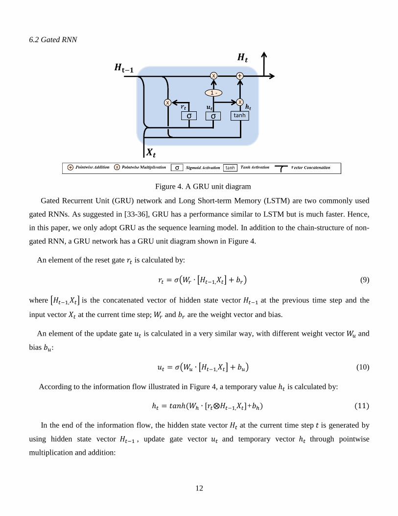
Figure 4. A GRU unit diagram
Gated Recurrent Unit (GRU) network and Long Short-term Memory (LSTM) are two commonly used
gated RNNs. As suggested in [33-36], GRU has a performance similar to LSTM but is much faster. Hence,
in this paper, we only adopt GRU as the sequence learning model. In addition to the chain-structure of non-
gated RNN, a GRU network has a GRU unit diagram shown in Figure 4.
An element of the reset gate is calculated by:
( [ ] ) (9)
where [ ] is the concatenated vector of hidden state vector at the previous time step and the
input vector at the current time step and are the weight vector and bias.
An element of the update gate is calculated in a very similar way, with different weight vector and
bias
( [ ] ) (10)
According to the information flow illustrated in Figure 4, a temporary value is calculated by:
+
In the end of the information flow, the hidden state vector at the current time step is generated by
using hidden state vector , update gate vector and temporary vector through pointwise
multiplication and addition:

13
(12)
Through (9)-(12), hidden state is updated from one time step to the next until the end of the sequence.
6.3 Sequential Configurations
A RNN can be implemented in different sequential configurations [30-31]. For the multi-year forecast
problem discussed in this paper, there are three suitable sequential configurations: Single-year Recursive,
Single-year with Interval and Multi-year Ahead. A 3-year load forecast is used as an example in here for
illustration purpose. The schematics of the three sequential configurations are shown in Figure 5.
Figure 5. Three different sequential configurations
The theoretical differences of these configurations lie in the network loss functions. For all neural
networks, network loss is converted to gradient and drives the training of neural network through back
propagation and mathematic chain-rule [22]. Here, Mean Absolute Error (MAE) is chosen to calculate the
network loss.
The Single-year Recursive configuration has been used in [19] and only forecasts the next one-year. This
means in order to forecast multiple years ahead, for example the next 3 years, the model has to be used
recursively: the first forecast year is firstly forecasted and then is used as a known input to forecast the
second forecast year ; similarly, is then used to forecast the third forecast year . Although this
configuration has a good performance for forecasting the first forecast year, the error may become larger for
later years especially when applying this configuration for a longer forecast window. This is because the
forecasted values are recursively used as input and the error can get accumulated as the forecast moves into
later years. This issue becomes more prominent if the feature fluctuation between neighbouring years is
large. The loss function of Single-year Recursive configuration is:

14
∑|
|
where is the training batch size; is the first forecast year ’s actual peak demand in record in the
training batch; is the first forecast year ’s forecasted peak demand in record in the training batch.
Different from the Single-year Recursive configurations, the Single-year with Interval configuration
directly forecasts a specific future year in the forecast window. When it is used to forecast the first forecast
year, it is equivalent to applying the Single-year Recursive configuration because the yearly interval is zero.
However, it becomes different for forecasting later years in the forecast window: for later years, the area and
feeder features between the forecast year and the current year are summed up to reflect the total change over
the interval years. Then the forecast year is directly forecasted. Compared to Single-year Recursive
configuration, applying this configuration is not a recursive process and can reduce error in many cases. The
trade-off is that for a forecast window of years, models need to be trained to forecast every different
year in the forecast window. The loss function for Single-year with Interval configuration is:
∑|
|
where is the training batch size;
is the forecast year’s actual peak demand in record in the
training batch;
is the forecast year’s forecasted peak demand in record in the training batch.
The example in Figure 5 shows the scenario when (i.e. forecasting the third forecast year); when
(i.e. forecasting the first forecast year), (14) is equivalent to (13).
Compared to the first two configurations, the Multi-year Ahead configuration outputs the results of
multiple years in the forecast window all at once. The advantage is its great efficiency and emphasis on the
holistic accuracy of the forecast window. On the other hand, it does not utilize the forecasted area and feeder
features in all future years (after the first forecast year). Using less information is not necessarily bad when
the accuracy of some information such as customer load information or far-out economic forecast cannot be
guaranteed. Its loss function is:
∑ ∑ |
|

15
where is the training batch size; is year’s actual peak demand in record in the training batch;
is year’s forecasted peak demand in record in the training batch; is the length of forecast window in
number of years. Different from and , measures the average error of the entire forecast window.
6.4 Sequential Datasets
To fit into the above three RNN sequential configurations, data records must be grouped by a fixed
number of time steps following specific formats. This is different from traditional single-row datasets that
are commonly used for other types of supervised learning methods. Table 2 to Table 4 are examples for
Single-year Recursive, Single-year with Interval and Multi-year Ahead configurations.
Table 2 shows a dataset example for Single-year Recursive configuration. Data record ID 21 is taken as
an example for explanation: in this record, the goal focuses on the forecast of 2011’s peak load by using the
previous-years’ base peak demand in 2008, 2009 and 2010 as well as the yearly economic and temperature
features in 2009, 2010 and 2011. EP1 and EP2 are the processed economic-population growth features after
applying PCA. ETAA is the “Extreme Temperature Above Average” feature and MCNLC is the “Major
Customer Net Load Change” feature as mentioned in Section 5. The third year 2011 is the forecast year and
its actual peak demand is also included in the training record.
Table 2: Dataset Example for Single-year Recursive Configuration
Data
Record
ID
Feeder
ID
Input
Year
Base Peak
Demand
Yearly Features Actual Peak
Demand
(Forecast Year) EP1 EP2 ETAA
MCNLC
… … … … … … … … …
21
0050 2009 433 A -0.64 0.44 0.7℃ 42 A 550 A
(2011) 0050 2010 502 A -0.16 0.31 -1.3℃ 34 A
0050 2011 554 A 0.33 -0.31 3.4℃ 0 A
22
0050 2010 502 A -0.16 0.31 -1.3℃ 34 A 521 A
(2012) 0050 2011 554 A 0.33 -0.31 3.4℃ 0 A
0050 2012 550 A -0.06 -0.17 -2.2℃ -21 A
… … … … … … … … …
Similarly, Table 3 shows a dataset example for Single-year with Interval configuration. Different from
Single-year Recursive configuration, the two data records aim to forecast 2012 and 2013 instead of the last
input year 2011; Table 4 shows a dataset example for Multi-year Ahead configuration. Taking data record
ID 35 as an example, the goal is not only to forecast 2011’s peak load but also the peak load in 2012 and
2013. The loss function takes all three years’ errors into consideration and is therefore less biased if 2011’s
loading experienced an unusual change. Compared to Single-year Recursive configuration, its focus on year
2011 is weaker as the goal is not only to forecast 2011 but also 2012 and 2013 all at once.

16
Table 3: Dataset Example for Single-year with Interval Configuration
Data
Record
ID
Feeder
ID
Input
Year
Base Peak
Demand
Yearly Features Actual Peak
Demand
(Forecast Year) EP1 EP2 ETAA
MCNLC
… … … … … … … … …
67
0050 2009 433 A -0.64 0.44 0.7℃ 42 A 521 A
(2012) 0050 2010 502 A -0.16 0.31 -1.3℃ 34 A
0050 2011 554 A 0.29 -0.50 -2.2℃ -21 A
68
0050 2009 433 A -0.64 0.44 0.7℃ 42 A 537 A
(2013) 0050 2010 502 A -0.16 0.31 -1.3℃ 34 A
0050 2011 554 A 0.07 0.28 1.8℃ 20 A
… … … … … … … … …
Table 4: Dataset Example for Multi-year Ahead Configuration
Data
Record
ID
Feeder
ID
Input
Year
Base Peak
Demand
Yearly Features Actual Peak
Demand
(Forecast Year) EP1 EP2 ETAA
MCNLC
… … … … … … … … …
35
0050 2009 433 A -0.64 0.44 0.7℃ 42 A 550 A (2011)
0050 2010 502 A -0.16 0.31 -1.3℃ 34 A 521 A (2012)
0050 2011 554 A 0.33 -0.31 3.4℃ 0 A 537 A (2013)
36
0050 2010 502 A -0.16 0.31 -1.3℃ 34 A 521 A (2012)
0050 2011 554 A 0.33 -0.31 3.4℃ 0 A 537 A (2013)
0050 2012 550 A -0.06 -0.17 -2.2℃ -21 A 549 A (2014)
… … … … … … … … …
7. Learning of Best-performing Sequential Configuration
For different feeders, the three sequential configurations presented in Section 6 may have different
performances depending on the input information. For example, the Single-year Recursive configuration
places all emphasis on the next one-year and can be accurate if the external drivers and customer load
information (including assumed values for future years) are accurate; Single-year with Interval configuration
can be effective when dealing with feeders with large yearly fluctuations as it reduces the error from the
recursive process; Multi-year Ahead configuration can be more accurate for saturated feeders which are less
sensitive to external drivers or feeders with less accurate customer load information.
However, it is challenging to manually analyze each feeder’s characteristics and picks the best-
performing sequential configuration for each feeder. This paper proposes an automatic way of learning the
best-performing Sequential Configuration for individual feeders based on historical data. Figure 6 shows a
training set example with 20-year data. The goal is to produce a three-year window forecast. This window
slides from the fourth year to eighteenth year and for each slide, a MAE is calculated for each sequential
configuration. Therefore, it produces in total 15 MAEs for performance evaluation.
17
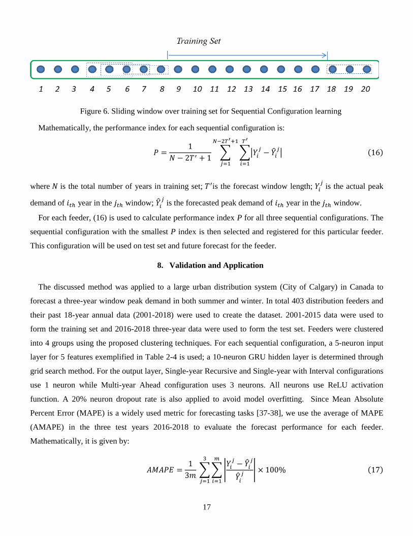
Figure 6. Sliding window over training set for Sequential Configuration learning
Mathematically, the performance index for each sequential configuration is:
∑ ∑|
|
where is the total number of years in training set; is the forecast window length; is the actual peak
demand of year in the window; is the forecasted peak demand of year in the window.
For each feeder, (16) is used to calculate performance index P for all three sequential configurations. The
sequential configuration with the smallest P index is then selected and registered for this particular feeder.
This configuration will be used on test set and future forecast for the feeder.
8. Validation and Application
The discussed method was applied to a large urban distribution system (City of Calgary) in Canada to
forecast a three-year window peak demand in both summer and winter. In total 403 distribution feeders and
their past 18-year annual data (2001-2018) were used to create the dataset. 2001-2015 data were used to
form the training set and 2016-2018 three-year data were used to form the test set. Feeders were clustered
into 4 groups using the proposed clustering techniques. For each sequential configuration, a 5-neuron input
layer for 5 features exemplified in Table 2-4 is used; a 10-neuron GRU hidden layer is determined through
grid search method. For the output layer, Single-year Recursive and Single-year with Interval configurations
use 1 neuron while Multi-year Ahead configuration uses 3 neurons. All neurons use ReLU activation
function. A 20% neuron dropout rate is also applied to avoid model overfitting. Since Mean Absolute
Percent Error (MAPE) is a widely used metric for forecasting tasks [37-38], we use the average of MAPE
(AMAPE) in the three test years 2016-2018 to evaluate the forecast performance for each feeder.
Mathematically, it is given by:
∑∑|
|

18
where is the number of feeders in the planning area; is the actual peak demand of feeder in year
(starting in 2016); is the forecasted peak demand of feeder in year.
In addition to AMAPE, two auxiliary metrics RMSE and (R-squared) are also used for performance
measurement [22,38]. Mathematically, they are given as below
√∑
∑ ( )
∑ ( )
where is the actual peak demand of testing record; is the predicted value corresponding to ; is
the average actual peak demand of all testing records; is the total number of testing records in three
years.
When , the prediction matches exactly with the actual every time in the test; when , the
performance is equivalent to always using the average of all actual values as prediction every time in the test;
if the prediction accuracy is even worse than blindly using the average of actual values, can become a
negative value. Different from AMAPE, RMSE and use absolute errors instead of percentage error for
performance measurement. As a result, their values can be affected by the absolute magnitude of power
demand and may not always align with AMAPE in comparison. This phenomenon has been observed in
Section 8.4.
8.1 Effect of Selective Sequence Learning
To test the effect of the proposed selective sequence learning (SSL) method, the proposed method is
compared to using only single sequential configurations for all feeders in summer and winter. The results
are shown in Figure 7.
19
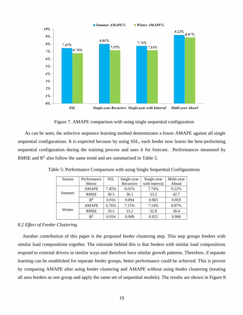
Figure 7. AMAPE comparison with using single sequential configuration
As can be seen, the selective sequence learning method demonstrates a lower AMAPE against all single
sequential configurations. It is expected because by using SSL, each feeder now learns the best-performing
sequential configuration during the training process and uses it for forecast. Performances measured by
RMSE and also follow the same trend and are summarized in Table 5.
Table 5: Performance Comparison with using Single Sequential Configurations
Season Performance
Metric
SSL Single-year
Recursive
Single-year
with Interval
Multi-year
Ahead
Summer AMAPE 7.45% 8.01% 7.74% 9.22%
RMSE 30.5 36.1 33.2 42.7
0.916 0.894 0.903 0.859
Winter AMAPE 6.76% 7.15% 7.14% 8.87%
RMSE 29.5 33.2 32.8 38.4
0.934 0.908 0.922 0.868
8.2 Effect of Feeder Clustering
Another contribution of this paper is the proposed feeder clustering step. This step groups feeders with
similar load compositions together. The rationale behind this is that feeders with similar load compositions
respond to external drivers in similar ways and therefore have similar growth patterns. Therefore, if separate
learning can be established for separate feeder groups, better performance could be achieved. This is proven
by comparing AMAPE after using feeder clustering and AMAPE without using feeder clustering (treating
all area feeders as one group and apply the same set of sequential models). The results are shown in Figure 8.

20
Figure 8. AMAPE comparison with and without feeder clustering
Performances measured by RMSE and also follow the same trend and are summarized in Table 6.
Table 6: Performance Comparison with and without Feeder Clustering
Season Performance Metric With Clutering Without Clustering
Summer AMAPE 7.45% 8.24%
RMSE 30.5 37.9
0.916 0.887
Winter AMAPE 6.76% 7.33%
RMSE 29.5 33.8
0.934 0.894
8.3 Comparison with Conventional Models
In the end, the proposed model was compared to various other models specified as below. To ensure
fairness, the same feature processing techniques discussed in Section 5 are also used for conventional
models. The hyper parameters for hidden layers used in the neural network based models are tuned through
grid search method.
Bottom-up model: as discussed in Section 2, this is the method to build a feeder load forecast based on
major customer load information. Mathematically, the “Major Customer Net Load Change” feature
from 2016 to 2018 was gathered and added to the previous year’s peak demand recursively to
approximately estimate the following year’s peak demand.
ARIMA model: for each feeder, its peak demand data between 2001 and 2015 was fed into an ARIMA
model for training. ARIMA (2,0,0) was chosen after experiments because it gave the best forecast result
among different ARIMA order parameters for the dataset. Then the peak demand values between 2016
and 2018 were calculated recursively.

21
One-input year recursive FNN (ORF): for each feeder, only one-input year’s features are used for
forecast. The features are the same as used in the proposed method, i.e. “Previous-Year Peak Demand”,
EP1, EP2, “Extreme Temperature over Average” and “Major Customer Net Load Change”. A
traditional FNN model is used, with a 5-neuron input layer, two 6-neuron hidden layers and a 1-neuron
output layer. Peak demand values between 2016 and 2018 were forecasted recursively.
Three-input year recursive FNN (TRF): a traditional FNN model is used to incorporate all the features
from three input years (in total 15 features) to forecast the third year’s peak demand. The FNN has a 15-
neuron input layer, two 10-neuron hidden layers and a 1-neuron output layer. Peak demand values
between 2016 and 2018 were forecasted recursively. The main difference between this method and the
proposed many-to-one sequence prediction is that it uses the FNN structure instead of RNN structure.
Three-input year non-recursive FNN (TNF): a traditional FNN model is used to incorporate all the
features from three input years (in total 15 features) to forecast the three forecast years’ peak demand.
The FNN has a 15-neuron input layer, two 12-neuron hidden layers and a 3-neuron output layer
representing peak demands in three years. Peak demand values between 2016 and 2018 were forecasted
all at the same time. The main difference between this method and the proposed shifted many-to-many
sequence prediction is that it uses the FNN structure instead of RNN structure.
Figure 9. AMAPE comparison with conventional models
The comparison is summarized in Figure 9. As can be seen, the proposed method outperforms all 5 non-
sequence prediction based conventional methods. Performances measured by RMSE and also follow the
same trend and are summarized in Table 7.

22
Table 7: Performance Comparison with Conventional Models
Season Performance Metric SSL Bottom-up ARIMA ORF TRF TNF
Summer AMAPE 7.45% 15.68% 13.44% 11.39% 10.04% 10.63%
RMSE 30.5 66.5 58.8 54.1 44.6 46.3
0.916 0.616 0.745 0.772 0.830 0.796
Winter AMAPE 6.76% 14.30% 11.91% 10.20% 9.25% 10.06%
RMSE 29.5 63.4 50.6 48.7 42.1 45.2
0.934 0.687 0.756 0.793 0.859 0.848
The superior performance of the proposed method (SSL) against other methods can be understood from
four perspectives: it effectively uses both area features and feeder features. In comparison, the bottom-up
and ARIMA methods can only use one aspect of information; it effectively use multiple historical years of
data for forecast. In comparison, ORF can only use one-year data; it uses a GRU based sequential learning
model. In comparison, TRF and TNF are based on regular FNN models and this network structure cannot
analyze the relationship of different years (timesteps); furthermore, the proposed method uses unsupervised
learning to pre-classify feeder types and selects the best sequential configuration for each feeder.
8.4 Performance in Each Cluster
As discussed above, the 403 feeders in the planning area were grouped into 4 clusters by load
composition. This section discusses the testing results for each cluster. The number of members in each
cluster, the load composition features of each cluster’s centroid and the 2016-2018 average loadings are
provided in Table 8.
Table 8: Cluster Composition
Feeder
Cluster ID ( ) of
Cluster Centroid
Number of
Cluster Members
Average Summer
Loading (A) Average Winter
Loading (A) 1 (77%,15%) 122 338 386
2 (30%,48%) 97 271 303
3 (21%,19%) 48 374 392
4 (27%,31%) 136 270 319
As can be seen from the second column in Table 8, the feeders in Cluster 1 have significantly more
residential load than commercial and industrial load; the feeders in Cluster 2 have more commercial load
than residential and industrial load; the feeders in Cluster 3 have significantly more industrial load than
residential and commercial load; the feeders in Cluster 4 have more balanced load types than in the other
three clusters, with comparable amount of residential, commercial and industrial load. The summer and
winter forecasting accuracies of these clusters measured by AMAPE are presented in Figure 10. It is shown
that Cluster 3 has relatively higher forecasting error. This is probably because Cluster 3 is industrial load
heavy and industrial load can fluctuate more drastically between years and operate in a more random pattern.

23
Figure 10. AMAPE comparison of different feeder clusters
Table 9: Performance Comparison with Different Clusters
Season Performance Metric Cluster 1 Cluster 2 Cluster 3 Cluster 4
Summer AMAPE 7.34% 7.01% 8.78% 7.46%
RMSE 31.3 23.1 41.2 28.2
0.829 0.870 0.708 0.840
Winter AMAPE 6.52% 6.30% 7.73% 6.95%
RMSE 30.1 21.7 38.1 28.6
0.850 0.929 0.783 0.862
However, it is noticed that RMSE and in Table 9 do not completely align with the observed trend
of AMAPE between different clusters. The exception is on Cluster 1 and Cluster 4: although Cluster
4’s AMAPE is slightly higher than Cluster 1, its performance measured by RMSE and is slightly
better than Cluster 1. This is because Cluster 4’s average loading is lower than Cluster 1 and results in
smaller absolute errors. Since RMSE and use absolute errors as shown in equation (18) and (19),
when the AMAPE difference between two clusters is small but the average loading difference is large,
the absolute error based comparison may not necessarily align with percentage based comparison
(AMAPE).
Furthermore, the numbers of sequential configurations registered within each cluster are checked and
summarized in Table 10.
Table 10: Best-performing Sequential Configurations Selected in Each Cluster
Feeder Cluster
ID
Number of
Cluster Members
Single-year
Recursive
Single-year
with Interval
Multi-year
Ahead
1 122 5 66 51
2 97 14 44 39
3 48 6 40 2
4 136 48 68 20
Total 403 73 218 112

24
As can be seen from Table 10, overall the least selected best-performing sequential configuration is the
Single-year Recursive Configuration. This is within expectation because this configuration suffers from the
recursive error for multi-year forecast; the most selected best-performing sequential configuration is the
Single-year with Interval Configuration. It is significantly better than the other two configurations,
especially for Cluster 3 when the load fluctuation between years is large due to its heavy industry load
presence; the Multi-year Ahead Configuration performs better when residential load is heavier in the
composition. This could be due to the fact that residential load is often more stable and less sensitive to
external economic drivers in later years.
8.5 Error Progression in Forecast Window
Figure 11. Performance comparison of different feeder clusters
The proposed method has been applied to the 403 feeders in the area in the testing period 2016-2018.
Figure 11 shows the AMAPE progression over the three-year forecast window for the feeder groups under
each best-performing configuration indicated in Table 6. It is found that the AMAPE for Single-year
Recursive configuration increases quickly in year 2 and year 3. This is again due to the recursive nature of
this configuration. In comparison, the other two configurations are much more stable. The AMAPE of
Single-year with Interval configuration only rises slightly because the area economic forecast itself is less
accurate in the later years of the forecast window. The AMAPE of Multi-year Ahead configuration is quite
stable because it is trained based on the overall accuracy of all three years in the forecast window and does
not rely on area features in the later years of the forecast window.
8.6 Application Resutls For Next 5 Years
In the end, the above models established based on historical data are applied to forecast the feeder peaks
of the next 5 years (2019 to 2023) in the same area. The average feeder peaks in 4 clusters for the next 5

25
years in summer and winter are presented in Figure 12. All 4 clusters of feeders experience load growth in
the next 5 years. Table 11 summarizes the average growth rates of the 5 years in both summer and winter.
Figure 12. Average forecast results for the next 5 years by feeder clusters
Table 11: Application Resutls For Next 5 Years
Feeder Cluster
ID
Summer Average
Growth Rate (%)
Winter Average
Growth Rate (%)
1 3.56 3.10
2 6.33 6.70
3 3.00 4.03
4 4.95 3.76
As Table 11 indicates, the growth of Cluster 2 (commercial heavy) is more rapid than the other 3 clusters
due to more expected commercial load developments in the area in the forecasting years. For example, a
major commercial development expected to energize in 2023 winter will increase the cluster loading
significantly. The gathered customer net load changes that are going to occur at different time points are
incorporated by the proposed model for different feeders and affect their loading growths over the
forecasting years. Also, it is observed that the winter loadings are generally higher than the summer loadings
across all clusters. This is because the tested planning area in Canada is a typical winter peaking system that
has more electricity consumed in winter months for heating purpose and the same load can consume
electricity differently between summer and winter seasons.
9. Conclusions and Discussions
This paper thoroughly discussed a novel method that can effectively forecast peak load of distribution
feeders in an area over multiple years in the future. Compared to the commonly used top-down and bottom-
up LTLF methods, as a hybrid forecasting method, the proposed method can seamlessly integrate top-down
area features and bottom-up feeder features to improve forecasting accuracy; also, compared to the existing
hybrid forecasting approach for area feeder LTLF, the proposed method:
uses sequential learning with three different sequential configurations to convert a multi-year LTLF
problem to a multi-timestep sequence prediction problem.

26
uses a novel configuration selection mechanism that can learn, register and apply the best sequential
configuration for each feeder in an area.
uses unsupervised learning techniques to automatically group feeders into different groups and
establish a set of sequence learning models for each group of feeders.
The proposed method was tested on a large urban distribution system in Canada. The results suggest:
Learning and applying best-performing sequential configurations for different feeders accordingly
provides better forecasting performance than applying single sequential configuration across all
feeders in a planning area;
Using clustering to help establish different learning models for different feeder groups in a planning
area can improve forecasting performance;
The proposed method successfully combines the top-down and bottom-up features in multiple
historical years for multi-year ahead LTLF. It proves the feasibility of converting a multi-year LTLF
problem to a multi-timestep sequence prediction problem.
The proposed method outperforms various conventional methods and the existing hybrid forecasting
method for the discussed problem.
In the future, when available, the proposed method should be tested on other area feeder datasets. The
research can also be expanded to other types of component-level energy forecasting problems such as
metering data forecast in a community. From the methodology improvement perspective, rather than using
PCA for feature engineering, other non-linear dimensionality reduction methods such as T-SNE, auto-
encoding as well as different feature selection methods can be considered and compared on the performance
in the future.
References
[1] H. L. Willis, Power Distribution Planning Reference Book, CRC press, 1997.
[2] F. Elkarmi, ed., Power System Planning Technologies and Applications: Concepts, Solutions and
Management, IGI Global, 2012.

27
[3] B. Stephen, X. Tang, P. R. Harvey, S. Galloway and K. I. Jennett, “Incorporating practice theory in sub-
profile models for short term aggregated residential load forecasting,” IEEE Transactions on Smart Grid,
vol. 8, no. 4, pp. 1591-1598, July 2017.
[4] Y. Wang, Q. Chen, M. Sun, C. Kang and Q. Xia, “An ensemble forecasting method for the aggregated
load with subprofiles,” IEEE Transactions on Smart Grid, vol. 9, no. 4, pp. 3906-3908, July 2018.
[5] Y. Goude, R. Nedellec and N. Kong, “Local short and middle term electricity load forecasting with semi-
parametric additive models,” IEEE Transactions on Smart Grid, vol. 5, no. 1, pp. 440-446, Jan. 2014.
[6] C. Li, Y. Tao, W. Ao, S. Yang and Y. Bai, “Improving forecasting accuracy of daily enterprise
electricity consumption using a random forest based on ensemble empirical mode decomposition,” Energy,
vol.165, pp. 1220-1227. .2018.
[7] X. Kong, C. Li, C. Wang, Y. Zhang and J. Zhang, “Short-term electrical load forecasting based on error
correction using dynamic mode decomposition,” Applied Energy, vol.261, p.114368, 2020.
[8] Y. Bai and C. Li, “Daily natural gas consumption forecasting based on a structure-calibrated support
vector regression approach”, Energy and Buildings, vol.127, pp.571-579, 2016.
[9] M. Malekizadeh, H. Karami, M. Karimi, A. Moshari and M. J. Sanjari, “Short-term load forecast using
ensemble neuro-fuzzy model,” Energy, vol.196, p.117127, 2020
[10] W. Simpson and D. Gotham, “Standard approaches to load forecasting and review of Manitoba Hydro
load forecast for needs for and alternatives To (NFAT),” The Manitoba Public Utilities Board, Winnipeg,
MB, Canada. [Online] http://www.pub.gov.mb.ca/nfat/pdf/load_forecast_simpson_gotham.pdf.
[11] T. Al-Saba and I. El-Amin, “Artificial neural networks as applied to long-term demand forecasting,”
Artificial Intelligence in Engineering, vol. 13, no. 2, pp.189-197, 1999.
[12] M. Askari and A. Fetanat, “Long-term load forecasting in power system: Grey system prediction-based
models,” Journal of Applied Sciences, vol. 11, no.16, pp. 3034-3038, 2011.
[13] F. Kong and G. Song, “Middle-long power load forecasting based on dynamic grey prediction and
support vector machine,” International Journal of Advanced Computer Technology, vol. 4, no. 5, pp. 148-156,
2012.

28
[14] L. Ekonomou, “Greek long-term energy consumption prediction using artificial neural networks,”
Energy, vol. 35, no. 2, pp.512-517, 2010.
[15] J. Wang, L. Li, D. Niu and Z. Tan, “An annual load forecasting model based on support vector
regression with differential evolution algorithm,” Applied Energy, vol. 94, pp.65-70, 2012.
[16] D. Burillo, M. V. Chester, S. Pincetl, E. D. Fournier and J. Reyna, “Forecasting peak electricity demand
for Los Angeles considering higher air temperatures due to climate change,” Applied Energy, vol. 236, pp.1-9,
2019.
[17] R. J. Hyndman and S. Fan, “Density forecasting for long-term peak electricity demand,” IEEE
Transactions on Power Systems, vol. 25, no. 2, pp. 1142-1153, May 2010.
[18] K. Train, J. Herriges and R. Windle, “Statistically adjusted engineering models of end-use load curves,”
Energy, vol. 10, no.10, pp. 1103-1111, 1985.
[19] M. Dong and L. S. Grumbach, “A Hybrid Distribution Feeder Long-Term Load Forecasting Method
Based on Sequence Prediction,” IEEE Transactions on Smart Grid, vol. 11, no. 1, pp. 470-482, Jan. 2020.
[20] R. Sun and C. L. Giles, “Sequence learning: from recognition and prediction to sequential decision
making,” IEEE Intelligent Systems, vol.16, no.4, pp. 67-70, July-Aug. 2001.
[21] M. Dong, “A Data-driven Long-term Dynamic Rating Estimating Method for Power Transformers,”
IEEE Transactions on Power Delivery, DOI: 10.1109/TPWRD.2020.2988921.
[22] I. H. Witten, E. Frank, M. A. Hall and C. J. Pal, Data Mining: Practical Machine Learning Tools and
Techniques, Morgan Kaufmann, 2016.
[23] J. A. Hartigan and M. A. Wong, “Algorithm AS 136: A K-means clustering algorithm,” Applied
Statistics, vol. 28, no. 1, pp. 100-108, 1979.
[24] P. J. Rousseeuw, “Silhouettes: a graphical aid to the interpretation and validation of cluster analysis,”
Journal of Computational and Applied Mathematics, vol. 20, pp.53-65, 1987.
[25] “Electricity use during cold snaps,” Hydro Quebec, Montreal, QB, Canada. [Online]
http://www.hydroquebec.com/residential/customer-space/electricity- use/winter-electricity-consumption.html.
[26] “Historical Climate Data,” Government of Canada, Canada. [Online] http://climate.weather.gc.ca/.
[27] “Distributed Energy Resources Customer Adoption Modeling with Combined Heat and Power
Application,” Berkeley Lab, Berkeley, CA, USA. [Online] https://escholarship.org/uc/item/874851f9.

29
[28] A. Soltani-Sobh, K. Heaslip, A. Stevanovic, R. Bosworth and D. Radivojevic, “Analysis of the Electric
Vehicles Adoption over the United States,” Transportation Research Procedia, vol.22, pp. 203-212, Jan.2017.
[29] J. F. Kolen and S. C. Kremer, “Gradient flow in recurrent nets: the difficulty of learning long-term
dependencies,” A Field Guide to Dynamical Recurrent Networks , IEEE, 2001.
[30] S. Hochreiter and J. Schmidhuber, “Long short-term memory,” Neural Computation, vol. 9, pp.1735-
1780, 1997.
[31] I. Sutskever, O. Vinyals and Q. V. Le. “Sequence to sequence learning with neural networks,” Advances
in Neural Information Processing Systems, pp. 3104-3112, 2014.
[32] K. Cho, B. Van Merriënboer, C. Gulcehre, D. Bahdanau, F. Bougares, H. Schwenk and Y. Bengio,
“Learning phrase representations using RNN encoder-decoder for statistical machine translation,” arXiv
Preprint, arXiv:1406.1078, 2014.
[33] J. Chung, C. Gulcehre, K. Cho and Y. Bengio, “Empirical evaluation of gated recurrent neural networks
on sequence modeling,” arXiv Preprint, arXiv:1412.3555, 2014.
[34] Y. Wang, M. Liu, Z. Bao and S. Zhang, “Short-term load forecasting with multi-source data using gated
recurrent unit neural networks,” Energies, vol. 11, no.5, p.1138, 2018
[35] M. Afrasiabi, M. Mohammadi, M. Rastegar and A. Kargarian, “Probabilistic deep neural network price
forecasting based on residential load and wind speed predictions,” IET Renewable Power Generation, vol. 13,
no. 11, pp. 1840-1848, 2019.
[36] X. Gao, X. Li, B. Zhao, W. Ji, X. Jing and Y. He, “Short-term electricity load forecasting model based
on EMD-GRU with feature selection,” Energies, vol. 12, no. 6, p.1140, 2019.
[37] K. B. Sahay and M. M. Tripathi, “Day ahead hourly load forecast of PJM electricity market and ISO
New England market by using artificial neural network,” IEEE ISGT 2014, Washington, DC, pp. 1-5, 2014.
[38] J. S. Armstrong and F. Collopy, “Error measures for generalizing about forecasting methods: empirical
comparisons,” International Journal of Forecasting, vol.8, no.1, pp.69-80,1992.