Multi-view 3D Object Reconstruction arXiv:1604.00449v1 [cs ... · 3D-R2N2 3 (a) Images of objects we wish to reconstruct (b) Overview of the network Fig.1. (a) Some sample images

3D-R2N2: A Unified Approach for Single andMulti-view 3D Object Reconstruction

Christopher B. Choy Danfei Xu? JunYoung Gwak?

Kevin Chen Silvio Savarese

Stanford University{chrischoy, danfei, jgwak, kchen92, ssilvio}@stanford.edu

Abstract. Inspired by the recent success of methods that employ shapepriors to achieve robust 3D reconstructions, we propose a novel recurrentneural network architecture that we call the 3D Recurrent Reconstruc-tion Neural Network (3D-R2N2). The network learns a mapping fromimages of objects to their underlying 3D shapes from a large collectionof synthetic data [1]. Our network takes in one or more images of an ob-ject instance from arbitrary viewpoints and outputs a reconstruction ofthe object in the form of a 3D occupancy grid. Unlike most of the previ-ous works, our network does not require any image annotations or objectclass labels for training or testing. Our extensive experimental analysisshows that our reconstruction framework i) outperforms the state-of-the-art methods for single view reconstruction, and ii) enables the 3D recon-struction of objects in situations when traditional SFM/SLAM methodsfail (because of lack of texture and/or wide baseline).

Keywords: multi-view, reconstruction, recurrent neural network

1 Introduction

Rapid and automatic 3D object prototyping has become a game-changing in-novation in many applications related to e-commerce, visualization, and archi-tecture, to name a few. This trend has been boosted now that 3D printing isa democratized technology and 3D acquisition methods are accurate and effi-cient [2]. Moreover, the trend is also coupled with the diffusion of large scalerepositories of 3D object models such as ShapeNet [1].

Most of the state-of-the-art methods for 3D object reconstruction, however,are subject to a number of restrictions. Some restrictions are that: i) objectsmust be observed from a dense number of views; or equivalently, views musthave a relatively small baseline. This is an issue when users wish to reconstructthe object from just a handful of views or ideally just one view (see Fig. 1(a));ii) objects’ appearances (or their reflectance functions) are expected to be Lam-bertian (i.e. non-reflective) and the albedos are supposed be non-uniform (i.e.,rich of non-homogeneous textures).

? indicates equal contribution.

arX

iv:1

604.

0044

9v1

[cs

.CV

] 2

Apr

201

6

2 C. B. Choy, D. Xu, J. Gwak, K. Chen, and S. Savarese

These restrictions stem from a number of key technical assumptions. Onetypical assumption is that features can be matched across views [3,4,5,6] ashypothesized by the majority of the methods based on SFM or SLAM [7,8]. It hasbeen demonstrated (for instance see [9]) that if the viewpoints are separated bya large baseline, establishing (traditional) feature correspondences is extremelyproblematic due to local appearance changes or self-occlusions. Moreover, lackof texture on objects and specular reflections also make the feature matchingproblem very difficult [10,11].

In order to circumvent issues related to large baselines or non-Lambertian sur-faces, 3D volumetric reconstruction methods such as space carving [12,13,14,15]and their probabilistic extensions [16] have become popular. These methods,however, assume that the objects are accurately segmented from the backgroundor that the cameras are calibrated, which is not the case in many applications.

A different philosophy is to assume that prior knowledge about the objectappearance and shape is available. The benefit of using priors is that the ensuingreconstruction method is less reliant on finding accurate feature correspondencesacross views. Thus, shape prior-based methods can work with fewer images andwith fewer assumptions on the object reflectance function as shown in [17,18].The shape priors are typically encoded in the form of simple 3D primitives asdemonstrated by early pioneering works [19,20] or learned from rich reposito-ries of 3D CAD models [21,22,23], whereby the concept of fitting 3D modelsto images of faces was explored to a much larger extent [24,25,26]. Sophisti-cated mathematical formulations have also been introduced to adapt 3D shapemodels to observations with different degrees of supervision [27] and differentregularization strategies [28].

This paper is in the same spirit as the methods discussed above, but with akey difference. Instead of trying to match a suitable 3D shape prior to the obser-vation of the object and possibly adapt to it, we use deep convolutional neuralnetworks to learn a mapping from observations to their underlying 3D shapes ofobjects from a large collection of training data. Inspired by early works that usedmachine learning to learn a 2D-to-3D mapping for scene understanding [29,30],data driven approaches have been recently proposed to solve the daunting prob-lem of recovering the shape of an object from just a single image [31,32] for agiven number of object categories. In our approach, however, we leverage for thefirst time the ability of deep neural networks to automatically learn, in a mereend-to-end fashion, the appropriate intermediate representations from data torecover approximated 3D object reconstructions from as few as a single imagewith minimal supervision.

Inspired by the success of Long Short-Term Memory (LSTM) [33] networks [34,35]as well as recent progress in single-view 3D reconstruction using ConvolutionalNeural Networks [36,37], we propose a novel architecture that we call the 3DRecurrent Reconstruction Neural Network (3D-R2N2). The network takes in oneor more images of an object instance from different viewpoints and outputs areconstruction of the object in the form of a 3D occupancy grid, as illustrated inFig. 1(b). Note that in both training and testing, our network does not require

3D-R2N2 3

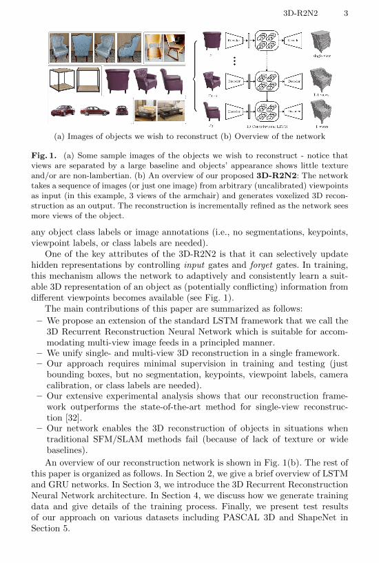
(a) Images of objects we wish to reconstruct (b) Overview of the network

Fig. 1. (a) Some sample images of the objects we wish to reconstruct - notice thatviews are separated by a large baseline and objects’ appearance shows little textureand/or are non-lambertian. (b) An overview of our proposed 3D-R2N2: The networktakes a sequence of images (or just one image) from arbitrary (uncalibrated) viewpointsas input (in this example, 3 views of the armchair) and generates voxelized 3D recon-struction as an output. The reconstruction is incrementally refined as the network seesmore views of the object.

any object class labels or image annotations (i.e., no segmentations, keypoints,viewpoint labels, or class labels are needed).

One of the key attributes of the 3D-R2N2 is that it can selectively updatehidden representations by controlling input gates and forget gates. In training,this mechanism allows the network to adaptively and consistently learn a suit-able 3D representation of an object as (potentially conflicting) information fromdifferent viewpoints becomes available (see Fig. 1).

The main contributions of this paper are summarized as follows:

– We propose an extension of the standard LSTM framework that we call the3D Recurrent Reconstruction Neural Network which is suitable for accom-modating multi-view image feeds in a principled manner.

– We unify single- and multi-view 3D reconstruction in a single framework.– Our approach requires minimal supervision in training and testing (just

bounding boxes, but no segmentation, keypoints, viewpoint labels, cameracalibration, or class labels are needed).

– Our extensive experimental analysis shows that our reconstruction frame-work outperforms the state-of-the-art method for single-view reconstruc-tion [32].

– Our network enables the 3D reconstruction of objects in situations whentraditional SFM/SLAM methods fail (because of lack of texture or widebaselines).

An overview of our reconstruction network is shown in Fig. 1(b). The rest ofthis paper is organized as follows. In Section 2, we give a brief overview of LSTMand GRU networks. In Section 3, we introduce the 3D Recurrent ReconstructionNeural Network architecture. In Section 4, we discuss how we generate trainingdata and give details of the training process. Finally, we present test resultsof our approach on various datasets including PASCAL 3D and ShapeNet inSection 5.


2 Recurrent Neural Network

In this section we provide a brief overview of Long Short-Term Memory (LSTM)networks and a variation of the LSTM called Gated Recurrent Units (GRU).

Long Short-Term Memory Unit. One of the most successful implemen-tations of the hidden states of an RNN is the Long Short Term Memory (LSTM)unit [33]. An LSTM unit explicitly controls the flow from input to output, allow-ing the network to overcome the vanishing gradient problem [33,38]. Specifically,an LSTM unit consists of four components: memory units (a memory cell anda hidden state), and three gates which control the flow of information from theinput to the hidden state (input gate), from the hidden state to the output(output gate), and from the previous hidden state to the current hidden state(forget gate). More formally, at time step t when a new input xt is received, theoperation of an LSTM unit can be expressed as:

it = σ(Wixt + Uiht−1 + bi) (1)

ft = σ(Wfxt + Ufht−1 + bf ) (2)

ot = σ(Woxt + Uoht−1 + bo) (3)

st = ft � st−1 + it � tanh(Wsxt + Usht−1 + bs) (4)

ht = ot � tanh(st) (5)

it, ft, ot refer to the input gate, the output gate, and the forget gate, respec-tively. st and ht refer to the memory cell and the hidden state, respectively. Weuse � to denote element-wise multiplication and the subscript t to refer to anactivation at time t. W(·), U(·) are matrices that transform the current input xtand the previous hidden state ht−1, respectively, and b(·) represents the biases.

Gated Recurrent Unit. A variation of the LSTM unit is the Gated Re-current Unit (GRU) proposed by Cho et al. [39]. An advantage of the GRU isthat there are fewer computations compared to the standard LSTM. In a GRU,an update gate controls both the input and forget gates. Another difference isthat a reset gate is applied before the nonlinear transformation. More formally,

ut = σ(WuT xt + Uu ∗ ht−1 + bf ) (6)

rt = σ(WiT xt + Ui ∗ ht−1 + bi) (7)

ht = (1− ut)� ht−1 + ut � tanh(Whxt + Uh(rt � ht−1) + bh) (8)

ut, rt, ht represent the update gate, the reset gate, and the hidden state re-spectively. We follow the same notations as LSTM for matrices and biases.

3 3D Recurrent Reconstruction Neural Network

In this section, we introduce a novel architecture named the 3D Recurrent Re-construction Network (3D-R2N2), which builds upon the standard LSTM andGRU. The goal of the network is to perform both single- and multi-view 3D

3D-R2N2 5

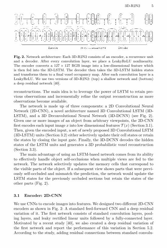
Fig. 2. Network architecture: Each 3D-R2N2 consists of an encoder, a recurrence unitand a decoder. After every convolution layer, we place a LeakyReLU nonlinearity.The encoder converts a 127 × 127 RGB image into a low-dimensional feature whichis then fed into the 3D-LSTM. The decoder then takes the 3D-LSTM hidden statesand transforms them to a final voxel occupancy map. After each convolution layer is aLeakyReLU. We use two versions of 3D-R2N2: (top) a shallow network and (bottom)a deep residual network [40].

reconstructions. The main idea is to leverage the power of LSTM to retain pre-vious observations and incrementally refine the output reconstruction as moreobservations become available.

The network is made up of three components: a 2D Convolutional NeuralNetwork (2D-CNN), a novel architecture named 3D Convolutional LSTM (3D-LSTM), and a 3D Deconvolutional Neural Network (3D-DCNN) (see Fig. 2).Given one or more images of an object from arbitrary viewpoints, the 2D-CNNfirst encodes each input image x into low dimensional features T (x) (Section 3.1).Then, given the encoded input, a set of newly proposed 3D Convolutional LSTM(3D-LSTM) units (Section 3.2) either selectively update their cell states or retainthe states by closing the input gate. Finally, the 3D-DCNN decodes the hiddenstates of the LSTM units and generates a 3D probabilistic voxel reconstruction(Section 3.3).

The main advantage of using an LSTM-based network comes from its abilityto effectively handle object self-occlusions when multiple views are fed to thenetwork. The network selectively updates the memory cells that correspond tothe visible parts of the object. If a subsequent view shows parts that were previ-ously self-occluded and mismatch the prediction, the network would update theLSTM states for the previously occluded sections but retain the states of theother parts (Fig. 2).

3.1 Encoder: 2D-CNN

We use CNNs to encode images into features. We designed two different 2D-CNNencoders as shown in Fig. 2: A standard feed-forward CNN and a deep residualvariation of it. The first network consists of standard convolution layers, pool-ing layers, and leaky rectified linear units followed by a fully-connected layer.Motivated by a recent study [40], we also created a deep residual variation ofthe first network and report the performance of this variation in Section 5.2.According to the study, adding residual connections between standard convolu-


tion layers effectively improves and speeds up the optimization process for verydeep networks. The deep residual variation of the encoder network has identitymapping connections after every 2 convolution layers except for the 4th pair. Tomatch the number of channels after convolutions, we use a 1× 1 convolution forresidual connections. The encoder output is then flattened and passed to a fullyconnected layer which compresses the output into a 1024 dimensional featurevector.

3.2 Recurrence: 3D Convolutional LSTM

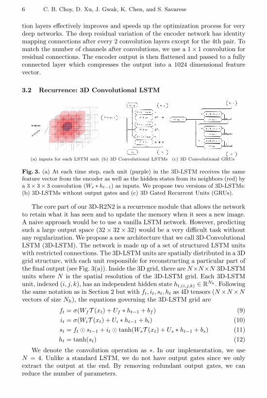
(a) inputs for each LSTM unit (b) 3D Convolutional LSTMs (c) 3D Convolutional GRUs

Fig. 3. (a) At each time step, each unit (purple) in the 3D-LSTM receives the samefeature vector from the encoder as well as the hidden states from its neighbors (red) bya 3× 3× 3 convolution (Ws ∗ ht−1) as inputs. We propose two versions of 3D-LSTMs:(b) 3D-LSTMs without output gates and (c) 3D Gated Recurrent Units (GRUs).

The core part of our 3D-R2N2 is a recurrence module that allows the networkto retain what it has seen and to update the memory when it sees a new image.A naive approach would be to use a vanilla LSTM network. However, predictingsuch a large output space (32× 32× 32) would be a very difficult task withoutany regularization. We propose a new architecture that we call 3D-ConvolutionalLSTM (3D-LSTM). The network is made up of a set of structured LSTM unitswith restricted connections. The 3D-LSTM units are spatially distributed in a 3Dgrid structure, with each unit responsible for reconstructing a particular part ofthe final output (see Fig. 3(a)). Inside the 3D grid, there are N×N×N 3D-LSTMunits where N is the spatial resolution of the 3D-LSTM grid. Each 3D-LSTMunit, indexed (i, j, k), has an independent hidden state ht,(i,j,k) ∈ RNh . Followingthe same notation as in Section 2 but with ft, it, st, ht as 4D tensors (N×N×Nvectors of size Nh), the equations governing the 3D-LSTM grid are

ft = σ(WfT (xt) + Uf ∗ ht−1 + bf ) (9)

it = σ(WiT (xt) + Ui ∗ ht−1 + bi) (10)

st = ft � st−1 + it � tanh(WsT (xt) + Us ∗ ht−1 + bs) (11)

ht = tanh(st) (12)

We denote the convolution operation as ∗. In our implementation, we useN = 4. Unlike a standard LSTM, we do not have output gates since we onlyextract the output at the end. By removing redundant output gates, we canreduce the number of parameters.

3D-R2N2 7

Intuitively, this configuration forces a 3D-LSTM unit to handle the mismatchbetween a particular region of the predicted reconstruction and the ground truthmodel such that each unit learns to reconstruct one part of the voxel space in-stead of contributing to the reconstruction of the entire space. This configurationalso endows the network with a sense of locality so that it can selectively updateits prediction about the previously occluded part of the object. We visualize suchbehavior in the appendix.

Moreover, a 3D Convolutional LSTM unit restricts the connections of its hid-den state to its spatial neighbors. For vanilla LSTMs, all elements in the hiddenlayer ht−1 affect the current hidden state ht, whereas a spatially structured 3DConvolutional LSTM only allows its hidden states ht,(i,j,k) to be affected by itsneighboring 3D-LSTM units for all i, j, and k. More specifically, the neighboringconnections are defined by the convolution kernel size. For instance, if we use a3×3×3 kernel, an LSTM unit is only affected by its immediate neighbors. Thisway, the units can share weights and the network can be further regularized.

In Section 2, we also described the Gated Recurrent Unit (GRU) as a varia-tion of the LSTM unit. We created a variation of the 3D-Convolutional LSTMusing Gated Recurrent Unit (GRU). More formally, a GRU-based recurrencemodule can be expressed as

ut = σ(WfxT (xt) + Uf ∗ ht−1 + bf ) (13)

rt = σ(WixT (xt) + Ui ∗ ht−1 + bi) (14)

ht = (1− ut)� ht−1 + ut � tanh(WhT (xt) + Uh ∗ (rt � ht−1) + bh) (15)

3.3 Decoder: 3D Deconvolutional Neural Network

After receiving an input image sequence x1, x2, · · · , xT , the 3D-LSTM passesthe hidden state hT to a decoder, which increases the hidden state resolution byapplying 3D convolutions, non-linearities, and 3D unpooling [41] until it reachesthe target output resolution.

As with the encoders, we propose a simple decoder network with 5 convo-lutions and a deep residual version with 4 residual connections followed by afinal convolution. After the last layer where the activation reaches the targetoutput resolution, we convert the final activation V ∈ RNvox×Nvox×Nvox×2 tothe occupancy probability p(i,j,k) of the voxel cell at (i, j, k) using voxel-wisesoftmax.

3.4 Loss: 3D Voxel-wise Softmax

The loss function of the network is defined as the sum of voxel-wise cross-entropy. Let the final output at each voxel (i, j, k) be Bernoulli distributions[1− p(i,j,k), p(i,j,k)], where the dependency on input X = {xt}t∈{1,...,T} is omit-ted, and let the corresponding ground truth occupancy be y(i,j,k) ∈ {0, 1}, then

L(X , y) =∑i,j,k

y(i,j,k) log(p(i,j,k)) + (1− y(i,j,k)) log(1− p(i,j,k)) (16)


4 Implementation

Data augmentation: In training, we used 3D CAD models for generatinginput images and ground truth voxel occupancy maps. We first rendered theCAD models with a transparent background and then augmented the inputimages with random crops from the PASCAL VOC 2012 dataset [42]. Also, wetinted the color of the models and randomly translated the images. Note thatall viewpoints were sampled randomly.Training: In training the network, we used variable length inputs ranging fromone image to an arbitrary number of images. More specifically, the input length(number of views) for each training example within a single mini-batch was keptconstant, but the input length of training examples across different mini-batchesvaried randomly. This enabled the network to perform both single- and multi-view reconstruction. During training, we computed the loss only at the end of aninput sequence in order to save both computational power and memory. On theother hand, during test time we could access the intermediate reconstructionsat each time step by extracting the hidden states of the LSTM units.Network: The input image size was set to 127 × 127. The output voxelizedreconstruction was of size 32 × 32 × 32. The networks used in the experimentswere trained for 60, 000 iterations with a batch size of 36 except for [Res3D-GRU-3] (See Table 1), which needed a batch size of 24 to fit in an NVIDIA Titan XGPU. For the LeakyReLU layers, the slope of the leak was set to 0.1 throughoutthe network. For deconvolution, we followed the unpooling scheme presentedin [41]. We used Theano [43] to implement our network and used Adam [44] forthe SGD update rule.

5 Experiments

In this section, we validate and demonstrate the capability of our approach withseveral experiments using the datasets described in Section 5.1. First, we showthe results of different variations of the 3D-R2N2 (Section 5.2). Next, we comparethe performance of our network on the PASCAL 3D [45] dataset with that ofa state-of-the-art method by Kar et al. [32] for single-view real-world imagereconstruction (Section 5.3). Then we show the network’s ability to performmulti-view reconstruction on the ShapeNet dataset [1] and the Online Productsdataset [46] (Section 5.4, Section 5.5). Finally, we compare our approach with aMulti View Stereo method on reconstructing objects with various texture levelsand viewpoint sparsity (Section 5.6).

5.1 Dataset

ShapeNet: The ShapeNet dataset is a collection of 3D CAD models that areorganized according to the WordNet hierarchy. We used a subset of the ShapeNetdataset which consists of 50,000 models and 13 major categories (see Table 5(c)for a complete list). We split the dataset into training and testing sets, with 4/5

3D-R2N2 9

for training and the remaining 1/5 for testing. We refer to these two datasets asthe ShapeNet training set and testing set throughout the experiments section.PASCAL 3D: The PASCAL 3D dataset is composed of PASCAL 2012 detec-tion images augmented with 3D CAD model alignment [45].Online Products: The dataset [46] contains images of 23,000 items sold online.MVS and SFM methods fail on these images due to ultra-wide baselines. Sincethe dataset does not have the ground-truth 3D CAD models, we only used thedataset for qualitative evaluation.MVS CAD Models: To compare our method with a Multi View Stereo method[47], we collected 4 different categories of high-quality CAD models. All CADmodels have texture-rich surfaces and were placed on top of a texture-rich paperto aid the camera localization of the MVS method.

Metrics: We used two metrics in evaluating the reconstruction quality. The pri-mary metric was the voxel Intersection-over-Union (IoU) between a 3D voxelreconstruction and its ground truth voxelized model. More formally,

IoU =∑i,j,k

[I(p(i,j,k) > t)I(y(i,j,k))

]/∑i,j,k

[I(I(p(i,j,k) > t) + I(y(i,j,k))

)](17)

where variables are defined in Section 3.4. I(·) is an indicator function andt is a voxelization threshold. Higher IoU values indicate better reconstructions.We also report the cross-entropy loss (Section 3.4) as a secondary metric. Lowerloss values indicate higher confidence reconstructions.

5.2 Network Structures Comparison

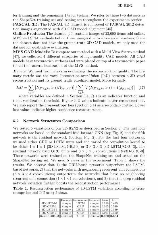
We tested 5 variations of our 3D-R2N2 as described in Section 3. The first fournetworks are based on the standard feed-forward CNN (top Fig. 2) and the fifthnetwork is the residual network (bottom Fig. 2). For the first four networks,we used either GRU or LSTM units and and varied the convolution kernel tobe either 1 × 1 × 1 [3D-LSTM/GRU-3] or 3 × 3 × 3 [3D-LSTM/GRU-3]. Theresidual network used GRU units and 3 × 3 × 3 convolutions [Res3D-GRU-3].These networks were trained on the ShapeNet training set and tested on theShapeNet testing set. We used 5 views in the experiment. Table 1 shows theresults. We observe that 1) the GRU-based networks outperform the LSTM-based networks, 2) that the networks with neighboring recurrent unit connections(3 × 3 × 3 convolutions) outperform the networks that have no neighboringrecurrent unit connection (1× 1× 1 convolutions), and 3) that the deep residualnetwork variation further boosts the reconstruction performance.

Table 1. Reconstruction performance of 3D-LSTM variations according to cross-entropy loss and IoU using 5 views.

Encoder Recurrence Decoder Loss IoU3D-LSTM-1 simple LSTM simple 0.116 0.4993D-GRU-1 simple GRU simple 0.105 0.540

3D-LSTM-3 simple LSTM simple 0.106 0.5393D-GRU-3 simple GRU simple 0.091 0.592

Res3D-GRU-3 residual GRU residual 0.080 0.634


5.3 Single Real-World Image Reconstruction

We evaluated the performance of our network in single-view reconstruction usingreal-world images, comparing the performance with that of a recent methodby Kar et al. [32]. To make a quantitative comparison, we used images fromthe PASCAL VOC 2012 dataset [42] and its corresponding 3D models from thePASCAL 3D+ dataset [45]. We ran the experiments with the same configurationas Kar et al. except that we allow the Kar et al. method to have ground-truthobject segmentation masks and keypoint labels as additional inputs for bothtraining and testing.

Input Ground Truth Ours Kar et al. [32] Input Ground Truth Ours Kar et al. [32]

(a)

Input Ground Truth Ours Kar et al. [32] Input Ground Truth Ours Kar et al. [32]

(b)

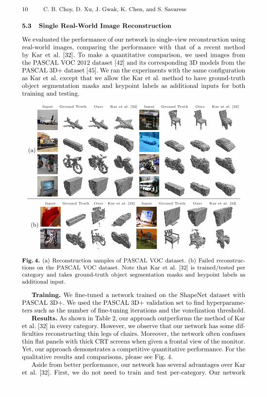
Fig. 4. (a) Reconstruction samples of PASCAL VOC dataset. (b) Failed reconstruc-tions on the PASCAL VOC dataset. Note that Kar et al. [32] is trained/tested percategory and takes ground-truth object segmentation masks and keypoint labels asadditional input.

Training. We fine-tuned a network trained on the ShapeNet dataset withPASCAL 3D+. We used the PASCAL 3D+ validation set to find hyperparame-ters such as the number of fine-tuning iterations and the voxelization threshold.

Results. As shown in Table 2, our approach outperforms the method of Karet al. [32] in every category. However, we observe that our network has some dif-ficulties reconstructing thin legs of chairs. Moreover, the network often confusesthin flat panels with thick CRT screens when given a frontal view of the monitor.Yet, our approach demonstrates a competitive quantitative performance. For thequalitative results and comparisons, please see Fig. 4.

Aside from better performance, our network has several advantages over Karet al. [32]. First, we do not need to train and test per-category. Our network

3D-R2N2 11

trains and reconstructs without knowing the object category. Second, our net-work does not require object segmentation masks and keypoint labels as addi-tional inputs. Kar et al. does demonstrate the possibility of testing on a wildunlabeled image by estimating the segmentation and keypoints. However, ournetwork outperforms their method tested with ground truth labels.

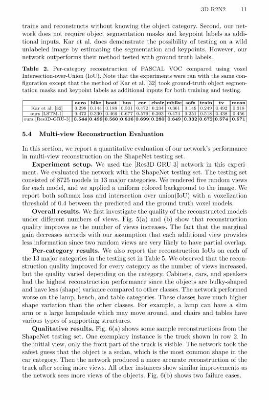
Table 2. Per-category reconstruction of PASCAL VOC compared using voxelIntersection-over-Union (IoU). Note that the experiments were ran with the same con-figuration except that the method of Kar et al. [32] took ground-truth object segmen-tation masks and keypoint labels as additional inputs for both training and testing.

aero bike boat bus car chair mbike sofa train tv meanKar et al. [32] 0.298 0.144 0.188 0.501 0.472 0.234 0.361 0.149 0.249 0.492 0.318ours [LSTM-1] 0.472 0.330 0.466 0.677 0.579 0.203 0.474 0.251 0.518 0.438 0.456

ours [Res3D-GRU-3] 0.544 0.499 0.560 0.816 0.699 0.280 0.649 0.332 0.672 0.574 0.571

5.4 Multi-view Reconstruction Evaluation

In this section, we report a quantitative evaluation of our network’s performancein multi-view reconstruction on the ShapeNet testing set.

Experiment setup. We used the [Res3D-GRU-3] network in this experi-ment. We evaluated the network with the ShapeNet testing set. The testing setconsisted of 8725 models in 13 major categories. We rendered five random viewsfor each model, and we applied a uniform colored background to the image. Wereport both softmax loss and intersection over union(IoU) with a voxelizationthreshold of 0.4 between the predicted and the ground truth voxel models.

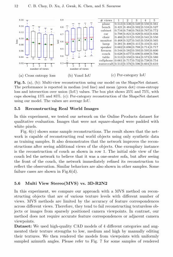
Overall results. We first investigate the quality of the reconstructed modelsunder different numbers of views. Fig. 5(a) and (b) show that reconstructionquality improves as the number of views increases. The fact that the marginalgain decreases accords with our assumption that each additional view providesless information since two random views are very likely to have partial overlap.

Per-category results. We also report the reconstruction IoUs on each ofthe 13 major categories in the testing set in Table 5. We observed that the recon-struction quality improved for every category as the number of views increased,but the quality varied depending on the category. Cabinets, cars, and speakershad the highest reconstruction performance since the objects are bulky-shapedand have less (shape) variance compared to other classes. The network performedworse on the lamp, bench, and table categories. These classes have much highershape variation than the other classes. For example, a lamp can have a slimarm or a large lampshade which may move around, and chairs and tables havevarious types of supporting structures.

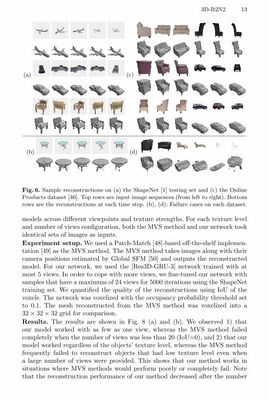
Qualitative results. Fig. 6(a) shows some sample reconstructions from theShapeNet testing set. One exemplary instance is the truck shown in row 2. Inthe initial view, only the front part of the truck is visible. The network took thesafest guess that the object is a sedan, which is the most common shape in thecar category. Then the network produced a more accurate reconstruction of thetruck after seeing more views. All other instances show similar improvements asthe network sees more views of the objects. Fig. 6(b) shows two failure cases.


1 2 3 4 5

number of views

0.02

0.04

0.06

0.08

0.10

0.12

0.14

0.16

loss

1 2 3 4 5

number of views

0.3

0.4

0.5

0.6

0.7

0.8

0.9

IoU

(a) Cross entropy loss (b) Voxel IoU

# views 1 2 3 4 5plane 0.513 0.536 0.549 0.556 0.561bench 0.421 0.484 0.502 0.516 0.527

cabinet 0.716 0.746 0.763 0.767 0.772car 0.798 0.821 0.829 0.833 0.836

chair 0.466 0.515 0.533 0.541 0.550monitor 0.468 0.527 0.545 0.558 0.565

lamp 0.381 0.406 0.415 0.416 0.421speaker 0.662 0.696 0.708 0.714 0.717firearm 0.544 0.582 0.593 0.595 0.600couch 0.628 0.677 0.690 0.698 0.706table 0.513 0.550 0.564 0.573 0.580

cellphone 0.661 0.717 0.732 0.738 0.754watercraft 0.513 0.576 0.596 0.604 0.610

(c) Per-category IoU

Fig. 5. (a), (b): Multi-view reconstruction using our model on the ShapeNet dataset.The performance is reported in median (red line) and mean (green dot) cross-entropyloss and intersection over union (IoU) values. The box plot shows 25% and 75%, withcaps showing 15% and 85%. (c): Per-category reconstruction of the ShapeNet datasetusing our model. The values are average IoU.

5.5 Reconstructing Real World Images

In this experiment, we tested our network on the Online Products dataset forqualitative evaluation. Images that were not square-shaped were padded withwhite pixels.

Fig. 6(c) shows some sample reconstructions. The result shows that the net-work is capable of reconstructing real world objects using only synthetic dataas training samples. It also demonstrates that the network improves the recon-structions after seeing additional views of the objects. One exemplary instanceis the reconstruction of couch as shown in row 1. The initial side view of thecouch led the network to believe that it was a one-seater sofa, but after seeingthe front of the couch, the network immediately refined its reconstruction toreflect the observation. Similar behaviors are also shown in other samples. Somefailure cases are shown in Fig.6(d).

5.6 Multi View Stereo(MVS) vs. 3D-R2N2

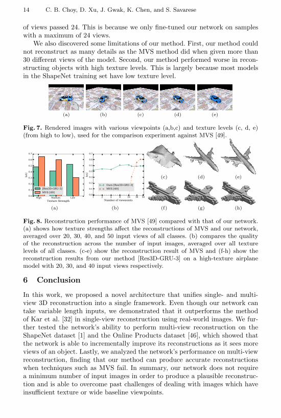
In this experiment, we compare our approach with a MVS method on recon-structing objects that are of various texture levels with different number ofviews. MVS methods are limited by the accuracy of feature correspondencesacross different views. Therefore, they tend to fail reconstructing textureless ob-jects or images from sparsely positioned camera viewpoints. In contrast, ourmethod does not require accurate feature correspondences or adjacent cameraviewpoints.Dataset: We used high-quality CAD models of 4 different categories and aug-mented their texture strengths to low, medium and high by manually editingtheir textures. We then rendered the models from viewpoints with uniformlysampled azimuth angles. Please refer to Fig. 7 for some samples of rendered

3D-R2N2 13

(a) (c)

(b) (d)

Fig. 6. Sample reconstructions on (a) the ShapeNet [1] testing set and (c) the OnlineProducts dataset [46]. Top rows are input image sequences (from left to right). Bottomrows are the reconstructions at each time step. (b), (d): Failure cases on each dataset.

models across different viewpoints and texture strengths. For each texture leveland number of views configuration, both the MVS method and our network tookidentical sets of images as inputs.

Experiment setup. We used a Patch-Match [48]-based off-the-shelf implemen-tation [49] as the MVS method. The MVS method takes images along with theircamera positions estimated by Global SFM [50] and outputs the reconstructedmodel. For our network, we used the [Res3D-GRU-3] network trained with atmost 5 views. In order to cope with more views, we fine-tuned our network withsamples that have a maximum of 24 views for 5000 iterations using the ShapeNettraining set. We quantified the quality of the reconstructions using IoU of thevoxels. The network was voxelized with the occupancy probability threshold setto 0.1. The mesh reconstructed from the MVS method was voxelized into a32× 32× 32 grid for comparison.

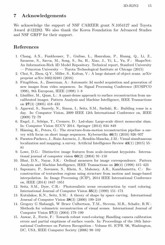
Results. The results are shown in Fig. 8 (a) and (b). We observed 1) thatour model worked with as few as one view, whereas the MVS method failedcompletely when the number of views was less than 20 (IoU=0), and 2) that ourmodel worked regardless of the objects’ texture level, whereas the MVS methodfrequently failed to reconstruct objects that had low texture level even whena large number of views were provided. This shows that our method works insituations where MVS methods would perform poorly or completely fail. Notethat the reconstruction performance of our method decreased after the number


of views passed 24. This is because we only fine-tuned our network on sampleswith a maximum of 24 views.

We also discovered some limitations of our method. First, our method couldnot reconstruct as many details as the MVS method did when given more than30 different views of the model. Second, our method performed worse in recon-structing objects with high texture levels. This is largely because most modelsin the ShapeNet training set have low texture level.

(a) (b) (c) (d) (e)

Fig. 7. Rendered images with various viewpoints (a,b,c) and texture levels (c, d, e)(from high to low), used for the comparison experiment against MVS [49].

(c) (d) (e)

(a) (b) (f) (g) (h)

Fig. 8. Reconstruction performance of MVS [49] compared with that of our network.(a) shows how texture strengths affect the reconstructions of MVS and our network,averaged over 20, 30, 40, and 50 input views of all classes. (b) compares the qualityof the reconstruction across the number of input images, averaged over all texturelevels of all classes. (c-e) show the reconstruction result of MVS and (f-h) show thereconstruction results from our method [Res3D-GRU-3] on a high-texture airplanemodel with 20, 30, and 40 input views respectively.

6 Conclusion

In this work, we proposed a novel architecture that unifies single- and multi-view 3D reconstruction into a single framework. Even though our network cantake variable length inputs, we demonstrated that it outperforms the methodof Kar et al. [32] in single-view reconstruction using real-world images. We fur-ther tested the network’s ability to perform multi-view reconstruction on theShapeNet dataset [1] and the Online Products dataset [46], which showed thatthe network is able to incrementally improve its reconstructions as it sees moreviews of an object. Lastly, we analyzed the network’s performance on multi-viewreconstruction, finding that our method can produce accurate reconstructionswhen techniques such as MVS fail. In summary, our network does not requirea minimum number of input images in order to produce a plausible reconstruc-tion and is able to overcome past challenges of dealing with images which haveinsufficient texture or wide baseline viewpoints.

3D-R2N2 15

7 Acknowledgements

We acknowledge the support of NSF CAREER grant N.1054127 and ToyotaAward #122282. We also thank the Korea Foundation for Advanced Studiesand NSF GRFP for their support.

References

1. Chang, A.X., Funkhouser, T., Guibas, L., Hanrahan, P., Huang, Q., Li, Z.,Savarese, S., Savva, M., Song, S., Su, H., Xiao, J., Yi, L., Yu, F.: ShapeNet:An Information-Rich 3D Model Repository. Technical report, Stanford University— Princeton University — Toyota Technological Institute at Chicago (2015)

2. Choi, S., Zhou, Q.Y., Miller, S., Koltun, V.: A large dataset of object scans. arXivpreprint arXiv:1602.02481 (2016)

3. Fitzgibbon, A., Zisserman, A.: Automatic 3d model acquisition and generation ofnew images from video sequences. In: Signal Processing Conference (EUSIPCO1998), 9th European, IEEE (1998) 1–8

4. Lhuillier, M., Quan, L.: A quasi-dense approach to surface reconstruction from un-calibrated images. Pattern Analysis and Machine Intelligence, IEEE Transactionson 27(3) (2005) 418–433

5. Agarwal, S., Snavely, N., Simon, I., Seitz, S.M., Szeliski, R.: Building rome in aday. In: Computer Vision, 2009 IEEE 12th International Conference on, IEEE(2009) 72–79

6. Engel, J., Schops, T., Cremers, D.: Lsd-slam: Large-scale direct monocular slam.In: Computer Vision–ECCV 2014. Springer (2014) 834–849

7. Haming, K., Peters, G.: The structure-from-motion reconstruction pipeline–a sur-vey with focus on short image sequences. Kybernetika 46(5) (2010) 926–937

8. Fuentes-Pacheco, J., Ruiz-Ascencio, J., Rendon-Mancha, J.M.: Visual simultaneouslocalization and mapping: a survey. Artificial Intelligence Review 43(1) (2015) 55–81

9. Lowe, D.G.: Distinctive image features from scale-invariant keypoints. Interna-tional journal of computer vision 60(2) (2004) 91–110

10. Bhat, D.N., Nayar, S.K.: Ordinal measures for image correspondence. PatternAnalysis and Machine Intelligence, IEEE Transactions on 20(4) (1998) 415–423

11. Saponaro, P., Sorensen, S., Rhein, S., Mahoney, A.R., Kambhamettu, C.: Re-construction of textureless regions using structure from motion and image-basedinterpolation. In: Image Processing (ICIP), 2014 IEEE International Conferenceon, IEEE (2014) 1847–1851

12. Seitz, S.M., Dyer, C.R.: Photorealistic scene reconstruction by voxel coloring.International Journal of Computer Vision 35(2) (1999) 151–173

13. Kutulakos, K.N., Seitz, S.M.: A theory of shape by space carving. InternationalJournal of Computer Vision 38(3) (2000) 199–218

14. Gregory G Slabaugh, W Bruce Culbertson, T.M., Stevens, M.R., Schafer, R.W.:Methods for volumetric reconstruction of visual scenes. International Journal ofComputer Vision 57(3) (2004) 179–199

15. Anwar, Z., Ferrie, F.: Towards robust voxel-coloring: Handling camera calibrationerrors and partial emptiness of surface voxels. In: Proceedings of the 18th Inter-national Conference on Pattern Recognition - Volume 01. ICPR ’06, Washington,DC, USA, IEEE Computer Society (2006) 98–102


16. Broadhurst, A., Drummond, T.W., Cipolla, R.: A probabilistic framework forspace carving. In: Computer Vision, 2001. ICCV 2001. Proceedings. Eighth IEEEInternational Conference on. Volume 1., IEEE (2001) 388–393

17. Dame, A., Prisacariu, V.A., Ren, C.Y., Reid, I.: Dense reconstruction using 3dobject shape priors. In: Computer Vision and Pattern Recognition (CVPR), 2013IEEE Conference on. (2013)

18. Bao, Y., chandraker, M., Lin, Y., Savarese, S.: Dense object reconstruction usingsemantic priors. In: Proceedings of the IEEE International Conference on Com-puter Vision and Pattern Recognition. (2013)

19. Lawrence, G.R.: Machine perception of three-dimensional solids. Ph. D. Thesis(1963)

20. Nevatia, R., Binford, T.O.: Description and recognition of curved objects. ArtificialIntelligence 8(1) (1977) 77–98

21. Zia, M.Z., Stark, M., Schiele, B., Schindler, K.: Detailed 3d representations forobject modeling and recognition, TPAMI (2013)

22. Rock, J., Gupta, T., Thorsen, J., Gwak, J., Shin, D., Hoiem, D.: Completing 3dobject shape from one depth image. In: Proceedings of the IEEE Conference onComputer Vision and Pattern Recognition. (2015) 2484–2493

23. Bongsoo Choy, C., Stark, M., Corbett-Davies, S., Savarese, S.: Enriching objectdetection with 2d-3d registration and continuous viewpoint estimation. In: TheIEEE Conference on Computer Vision and Pattern Recognition (CVPR). (June2015)

24. Blanz, V., Vetter, T.: Face recognition based on fitting a 3d morphable model.Pattern Analysis and Machine Intelligence, IEEE Transactions on 25(9) (2003)1063–1074

25. Matthews, I., Xiao, J., Baker, S.: 2d vs. 3d deformable face models: Representa-tional power, construction, and real-time fitting. International journal of computervision 75(1) (2007) 93–113

26. Kemelmacher-Shlizerman, I., Basri, R.: 3d face reconstruction from a single imageusing a single reference face shape. Pattern Analysis and Machine Intelligence,IEEE Transactions on 33(2) (2011) 394–405

27. Prisacariu, V.A., Segal, A.V., Reid, I.: Simultaneous monocular 2d segmenta-tion, 3d pose recovery and 3d reconstruction. In: Computer Vision–ACCV 2012.Springer (2012) 593–606

28. Sandhu, R., Dambreville, S., Yezzi, A., Tannenbaum, A.: A nonrigid kernel-basedframework for 2d-3d pose estimation and 2d image segmentation. Pattern Analysisand Machine Intelligence, IEEE Transactions on 33(6) (2011) 1098–1115

29. Saxena, A., Sun, M., Ng, A.Y.: Make3d: Learning 3d scene structure from a singlestill image. IEEE Trans. Pattern Anal. Mach. Intell. 31(5) (may 2009) 824–840

30. Hoiem, D., Efros, A.A., Hebert, M.: Automatic photo pop-up. ACM transactionson graphics (TOG) 24(3) (2005) 577–584

31. Vicente, S., Carreira, J., Agapito, L., Batista, J.: Reconstructing pascal voc. In:The IEEE Conference on Computer Vision and Pattern Recognition (CVPR).(2014)

32. Kar, A., Tulsiani, S., Carreira, J., Malik, J.: Category-specific object reconstructionfrom a single image. In: Computer Vision and Pattern Recognition (CVPR), 2015IEEE Conference on, IEEE (2015) 1966–1974

33. Hochreiter, S., Schmidhuber, J.: Long short-term memory. Neural Comput. 9(8)(November 1997) 1735–1780

34. Sundermeyer, M., Schluter, R., Ney, H.: Lstm neural networks for language mod-eling. In: INTERSPEECH. (2012) 194–197

3D-R2N2 17

35. Sutskever, I., Vinyals, O., Le, Q.V.: Sequence to sequence learning with neuralnetworks. In: Advances in neural information processing systems. (2014) 3104–3112

36. Eigen, D., Puhrsch, C., Fergus, R.: Depth map prediction from a single imageusing a multi-scale deep network. In: Advances in Neural Information ProcessingSystems 27. (2014)

37. Liu, F., Shen, C., Lin, G.: Deep convolutional neural fields for depth estimationfrom a single image. In: Proc. IEEE Conf. Computer Vision and Pattern Recog-nition. (2015)

38. Bengio, Y., Simard, P., Frasconi, P.: Learning long-term dependencies with gradi-ent descent is difficult. IEEE Transactions on Neural Networks 5(2) (Mar 1994)157–166

39. Cho, K., van Merrienboer, B., Gulcehre, C., Bahdanau, D., Bougares, F., Schwenk,H., Bengio, Y.: Learning Phrase Representations using RNN Encoder-Decoder forStatistical Machine Translation. ArXiv e-prints (2014)

40. He, K., Zhang, X., Ren, S., Sun, J.: Deep Residual Learning for Image Recognition.ArXiv e-prints (December 2015)

41. A.Dosovitskiy, J.T.Springenberg, T.Brox: Learning to generate chairs with convo-lutional neural networks. In: IEEE International Conference on Computer Visionand Pattern Recognition (CVPR). (2015)

42. Everingham, M., Van Gool, L., Williams, C., Winn, J., Zisserman, A.: The pascalvisual object classes challenge 2012 (2011)

43. Bergstra, J., Breuleux, O., Bastien, F., Lamblin, P., Pascanu, R., Desjardins, G.,Turian, J., Warde-Farley, D., Bengio, Y.: Theano: a CPU and GPU math expres-sion compiler. In: Proceedings of the Python for Scientific Computing Conference(SciPy). (June 2010)

44. Kingma, D., Ba, J.: Adam: A Method for Stochastic Optimization. ArXiv e-prints(2014)

45. Xiang, Y., Mottaghi, R., Savarese, S.: Beyond pascal: A benchmark for 3d objectdetection in the wild. In: Applications of Computer Vision (WACV), 2014 IEEEWinter Conference on, IEEE (2014) 75–82

46. Song, H.O., Xiang, Y., Jegelka, S., Savarese, S.: Deep metric learning via liftedstructured feature embedding. ArXiv e-prints (2015)

47. : Cg studio (2016) [Online; accessed 14-March-2016].48. Barnes, C., Shechtman, E., Finkelstein, A., Goldman, D.: Patchmatch: A random-

ized correspondence algorithm for structural image editing. ACM Transactions onGraphics-TOG 28(3) (2009) 24

49. : Openmvs: open multi-view stereo reconstruction library (2015) [Online; accessed14-March-2016].

50. Moulon, P., Monasse, P., Marlet, R.: Global fusion of relative motions for ro-bust, accurate and scalable structure from motion. In: Proceedings of the IEEEInternational Conference on Computer Vision. (2013) 3248–3255

Documents

Multi-view 3D Object Reconstruction arXiv:1604.00449v1 [cs ... · 3D-R2N2 3 (a) Images of objects we wish to reconstruct (b) Overview of the network Fig.1. (a) Some sample images