Embed Size (px)
Citation preview

MULTI-TERMINAL SECRECY AND SOURCE CODING
A DISSERTATION
SUBMITTED TO THE DEPARTMENT OF ELECTRICAL
ENGINEERING
AND THE COMMITTEE ON GRADUATE STUDIES
OF STANFORD UNIVERSITY
IN PARTIAL FULFILLMENT OF THE REQUIREMENTS
FOR THE DEGREE OF
DOCTOR OF PHILOSOPHY
Yeow-Khiang Chia
December 2011

http://creativecommons.org/licenses/by-nc/3.0/us/
This dissertation is online at: http://purl.stanford.edu/jh787xk7499
© 2011 by Yeow Khiang Chia. All Rights Reserved.
Re-distributed by Stanford University under license with the author.
This work is licensed under a Creative Commons Attribution-Noncommercial 3.0 United States License.
ii

I certify that I have read this dissertation and that, in my opinion, it is fully adequatein scope and quality as a dissertation for the degree of Doctor of Philosophy.
Abbas El-Gamal, Primary Adviser
I certify that I have read this dissertation and that, in my opinion, it is fully adequatein scope and quality as a dissertation for the degree of Doctor of Philosophy.
Thomas Cover
I certify that I have read this dissertation and that, in my opinion, it is fully adequatein scope and quality as a dissertation for the degree of Doctor of Philosophy.
Itschak Weissman
Approved for the Stanford University Committee on Graduate Studies.
Patricia J. Gumport, Vice Provost Graduate Education
This signature page was generated electronically upon submission of this dissertation in electronic format. An original signed hard copy of the signature page is on file inUniversity Archives.
iii

Yeow-Khiang Chia
I certify that I have read this dissertation and that, in my opinion, it
is fully adequate in scope and quality as a dissertation for the degree
of Doctor of Philosophy.
(Abbas El Gamal) Principal Adviser
I certify that I have read this dissertation and that, in my opinion, it
is fully adequate in scope and quality as a dissertation for the degree
of Doctor of Philosophy.
(Tsachy Weissman)
I certify that I have read this dissertation and that, in my opinion, it
is fully adequate in scope and quality as a dissertation for the degree
of Doctor of Philosophy.
(Thomas Cover)
Approved for the University Committee on Graduate Studies
Preface
Network Information Theory is a branch of Information Theory that aims to address
the fundamental limits of communications in a multiple user setting and when several
sources of information are available. While a complete theory is still lacking, tools and
techniques developed to address research problems in Network Information Theory
have started to make an impact on other fields.
In this thesis, we present results in two sub-areas in Network Information The-
ory. The first area, Information-Theoretic Secrecy, involves an application of Network
Information Theory techniques to a secret communication setting, where a message
is to be kept hidden from an eavesdropper. We consider two generalizations of the
classical wiretap channel, where a sender wishes to communicate to a receiver over
a noisy broadcast channel in the presence of an eavesdropper. The first generaliza-
tion considers the setting where we have more than one receiver or more than one
eavesdropper. The second setting considers the case where the transmission occurs
over a broadcast channel with state - a channel model that can serve a base model
for communicating over fast fading channels found in wireless communications.
In the second part of this thesis, we turn our attention to the area of multi-terminal
source coding. In particular, we investigate the Cascade Source Coding problem
where a source node has a source sequence that it wishes to send to an intermediate
node over a rate limited link, and also to an end node that the intermediate node
can communicate with over a rate limited link. We investigate the optimum coding
schemes under different assumptions on the side information available at the nodes,
or operational restrictions on the reconstruction process.

Acknowledgements
I am grateful to my adviser Professor Abbas El Gamal, who taught me most of what
I know about Network Information Theory through our interactions, his EE476 class
and his upcoming book on this subject. In addition, he has also taught me most of
what I know about research in general. The breath and depth of his research work is
inspiring, and I hope that I will be able to emulate it someday.
I am also grateful to my co-adviser Professor Tsachy Weissman, who has also
taught me a lot about Information Theory. I had the pleasure of learning about
universal schemes in Information Theory from his EE477 class, and about the rela-
tionship between estimation, mutual information and divergence through our joint
work. I have also benefited much from his group meetings.
Some of the fun times I had in Stanford were in Professor Thomas Cover’s research
seminars, and I thank him for giving me the opportunity to attend his research
seminars, where I got to know many interesting puzzles, facets of Information Theory,
Mathematics, sports and life in general. The insights and ideas I obtained from his
research seminars are too broad to list out, but just to name one, I think I now know
how to gamble in certain situations, such as when I am faced with a Saint Petersburg’s
Paradox.
I have benefited greatly from my interactions with the past and present students
at the Information Systems Laboratory and I thank them for it. In particular, I
would like to thank Idoia Ochoa Alvarez, Himanshu Asnani, Bernd Bandemer, Bob-
bie Glen Chern, Paul Cuff, Shirin Jalali, Young-Han Kim, Joseph Koo, Gowtham
Kumar, Alexandros Manolakos, Taesup Moon, Vinith Misra, Chandra Nair, Albert
No, Haim Permuter, Han-I Su, Kartik Venkat and Lei Zhao. I would also like to

thank Kelly, our group’s administrative assistant, for her efficiency and knowledge in
various administrative matters.
My experience in Stanford has been greatly enriched by several visiting students
and researchers. I would like to thank the visitors, especially Rajiv Soundararajan
and Majid Khormuji, for many interesting discussions. I was also fortunate to be able
to visit Professor Zhang Lin’s group at Tsinghua University for research exchange,
and I would like to thank Professor Zhang Lin and his students for hosting me.
Outside of research, I was fortunate to make some good friends in Stanford and,
in particular, I would like to thank Vijay Chandrasekhar, Issac Lim, Christopher
Philips, Lieven Verslegers, Karthik Vijayraghavan and Yang Wang for their friendship
and times we spent together.
Finally, and most importantly, I thank my wife, Hwee-Hoon, for her constant
encouragement, love and support, without which my journey in Stanford would not
have been possible.

Contents
Preface
Acknowledgements
1 Introduction 1
1.1 Information-Theoretic Secrecy . . . . . . . . . . . . . . . . . . . . . . 1
1.2 Cascade Source Coding . . . . . . . . . . . . . . . . . . . . . . . . . . 5
2 3 Receivers Wiretap channel 8
2.1 Introduction to 3-receivers Wiretap Channel . . . . . . . . . . . . . . 8
2.2 Definitions and Problem Setup . . . . . . . . . . . . . . . . . . . . . . 11
2.2.1 2-Receivers, 1-Eavesdropper . . . . . . . . . . . . . . . . . . . 11
2.2.2 1-Receiver, 2-Eavesdroppers . . . . . . . . . . . . . . . . . . . 12
2.3 2-receiver wiretap channel . . . . . . . . . . . . . . . . . . . . . . . . 13
2.4 2-receivers, 1-eavesdropper wiretap channel . . . . . . . . . . . . . . . 16
2.4.1 Asymptotic perfect secrecy . . . . . . . . . . . . . . . . . . . . 17
2.4.2 2-Receivers, 1-Eavesdropper with Common Message . . . . . . 28
2.5 1-receiver, 2-eavesdroppers wiretap channel . . . . . . . . . . . . . . . 35
2.6 Summary of Chapter . . . . . . . . . . . . . . . . . . . . . . . . . . . 42
3 Wiretap Channel with state 44
3.1 Introduction to Wiretap Channel with Causal State Information . . . 44
3.2 Problem Definition . . . . . . . . . . . . . . . . . . . . . . . . . . . . 46
3.3 Summary of Main Results . . . . . . . . . . . . . . . . . . . . . . . . 47
3.4 Proof of Theorem 3.1 . . . . . . . . . . . . . . . . . . . . . . . . . . . 55
3.5 Proof of Theorem 3.2 . . . . . . . . . . . . . . . . . . . . . . . . . . . 68
3.6 Summary of Chapter . . . . . . . . . . . . . . . . . . . . . . . . . . . 70
4 Cascade and Triangular Source Coding 71
4.1 Introduction to Cascade and Triangular Source Coding . . . . . . . . 71
4.2 Problem Definition . . . . . . . . . . . . . . . . . . . . . . . . . . . . 75
4.2.1 Cascade and Triangular Source coding . . . . . . . . . . . . . 75
4.2.2 Two way Cascade and Triangular Source Coding . . . . . . . 76
4.3 Main results . . . . . . . . . . . . . . . . . . . . . . . . . . . . . . . . 77
4.3.1 Cascade Source Coding . . . . . . . . . . . . . . . . . . . . . . 78
4.3.2 Triangular Source Coding . . . . . . . . . . . . . . . . . . . . 81
4.3.3 Two Way Cascade Source Coding . . . . . . . . . . . . . . . . 84
4.3.4 Two Way Triangular Source Coding . . . . . . . . . . . . . . . 90
4.4 Quadratic Gaussian Distortion Case . . . . . . . . . . . . . . . . . . . 94
4.4.1 Quadratic Gaussian Cascade Source Coding . . . . . . . . . . 94
4.4.2 Quadratic Gaussian Triangular Source Coding . . . . . . . . . 96
4.4.3 Quadratic Gaussian Two Way Source Coding . . . . . . . . . 98
4.5 Triangular Source Coding with a helper . . . . . . . . . . . . . . . . . 106
4.6 Summary of Chapter . . . . . . . . . . . . . . . . . . . . . . . . . . . 109
5 Causal Cascade and Triangular S.C. 111
5.1 Introduction to Cascade and Triangular Source Coding with causality
constraints . . . . . . . . . . . . . . . . . . . . . . . . . . . . . . . . . 111
5.2 Problem Definition . . . . . . . . . . . . . . . . . . . . . . . . . . . . 112
5.2.1 Causal Cascade and Triangular Source coding with same side
information at first 2 nodes . . . . . . . . . . . . . . . . . . . 113
5.2.2 Lossless Causal Cascade Source Coding . . . . . . . . . . . . . 114
5.3 Causal Cascade and Triangular Source coding with same side informa-
tion at first 2 nodes . . . . . . . . . . . . . . . . . . . . . . . . . . . . 115
5.3.1 Causal Cascade Source Coding . . . . . . . . . . . . . . . . . 115
5.3.2 Causal Triangular Source Coding . . . . . . . . . . . . . . . . 118

5.4 Lossless Causal Cascade Source Coding . . . . . . . . . . . . . . . . . 119
5.5 Summary of Chapter . . . . . . . . . . . . . . . . . . . . . . . . . . . 124
6 Conclusions 125
A Proofs for Chapter 2 127
A.1 Proof of Lemma 2.1 . . . . . . . . . . . . . . . . . . . . . . . . . . . . 127
A.2 Evaluation for example . . . . . . . . . . . . . . . . . . . . . . . . . . 129
A.3 Proof of Theorem 2.2 . . . . . . . . . . . . . . . . . . . . . . . . . . . 133
A.4 Converse for Proposition 2.2 . . . . . . . . . . . . . . . . . . . . . . . 135
A.5 Proof of Proposition 2.3 . . . . . . . . . . . . . . . . . . . . . . . . . 136
A.6 Proof of Proposition 2.4 . . . . . . . . . . . . . . . . . . . . . . . . . 138
B Proofs for Chapter 3 143
B.1 Proof of Proposition 3.1 . . . . . . . . . . . . . . . . . . . . . . . . . 143
B.2 Proof of Proposition 3.2 . . . . . . . . . . . . . . . . . . . . . . . . . 147
B.3 Proof of Proposition 3.3 . . . . . . . . . . . . . . . . . . . . . . . . . 149
C Proofs for Chapter 4 151
C.1 Achievability proof of Theorem 4.1 . . . . . . . . . . . . . . . . . . . 151
C.2 Achievability proof of Theorem 4.2 . . . . . . . . . . . . . . . . . . . 154
C.3 Achievability proof of Theorem 4.3 . . . . . . . . . . . . . . . . . . . 156
C.4 Achievability proof of Theorem 4.4 . . . . . . . . . . . . . . . . . . . 158
C.5 Cardinality Bounds . . . . . . . . . . . . . . . . . . . . . . . . . . . . 158
C.6 Alternative characterizations of rate distortion regions in Corollar-
ies 4.1 and 4.2 . . . . . . . . . . . . . . . . . . . . . . . . . . . . . . . 160
C.7 Proof of Converse for Triangular source coding with helper . . . . . . 162
Bibliography 165

List of Tables

List of Figures
1.1 Wiretap Channel: The encoder wishes to send a message to the decoder
so that the decoder receives the message with high probability, while
keeping it secret from the eavesdropper. Specifically, we require that
limn→∞ I(M ;Zn) = 0. . . . . . . . . . . . . . . . . . . . . . . . . . . 2
1.2 Special case of setting consider in Chapter 2. Here, we wish to send a
confidential message to both decoders 1 (Y n1 ) and 2 (Y n
2 ) while keeping
it secret from the eavesdropper. . . . . . . . . . . . . . . . . . . . . . 3
1.3 Wiretap channel with State . . . . . . . . . . . . . . . . . . . . . . . 4
1.4 Cascade source coding setting . . . . . . . . . . . . . . . . . . . . . . 5
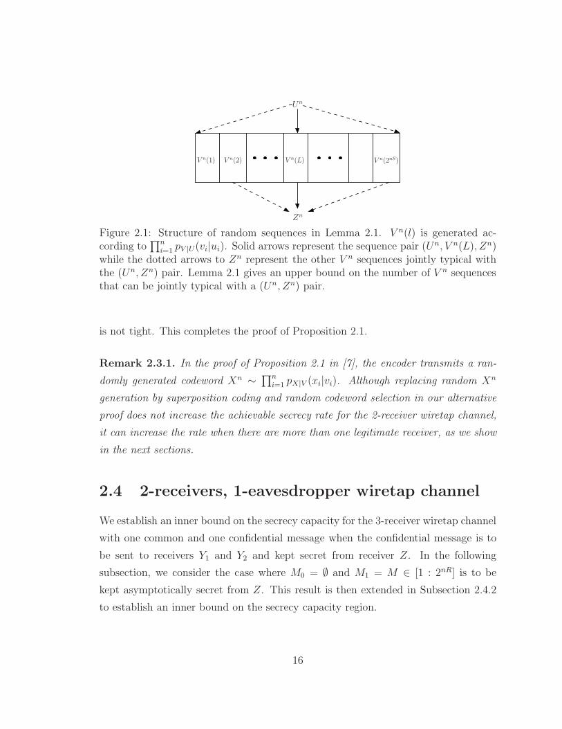
2.1 Structure of random sequences in Lemma 2.1. V n(l) is generated ac-
cording to∏n
i=1 pV |U(vi|ui). Solid arrows represent the sequence pair
(Un, V n(L), Zn) while the dotted arrows to Zn represent the other V n
sequences jointly typical with the (Un, Zn) pair. Lemma 2.1 gives an
upper bound on the number of V n sequences that can be jointly typical
with a (Un, Zn) pair. . . . . . . . . . . . . . . . . . . . . . . . . . . . 16
2.2 Multilevel broadcast channel . . . . . . . . . . . . . . . . . . . . . . . 20
3.1 Wiretap channel with State . . . . . . . . . . . . . . . . . . . . . . . 45
3.2 Example . . . . . . . . . . . . . . . . . . . . . . . . . . . . . . . . . . 49
3.3 Encoding in block j. . . . . . . . . . . . . . . . . . . . . . . . . . . . 52
4.1 Cascade source coding setting . . . . . . . . . . . . . . . . . . . . . . 72
4.2 Triangular source coding setting. . . . . . . . . . . . . . . . . . . . . 72

4.3 Setup for two way cascade source coding. . . . . . . . . . . . . . . . . 74
4.4 Setup for two way triangular source coding. . . . . . . . . . . . . . . 74
4.5 Extended Quadratic Gaussian Two Way source coding . . . . . . . . 99
4.6 Setup for analysis of achievability of backward rates . . . . . . . . . . 101
4.7 Triangular Source Coding with a helper . . . . . . . . . . . . . . . . . 106
5.1 Triangular source coding setting. If R3 = 0, this setting reduces to the
Cascade setting . . . . . . . . . . . . . . . . . . . . . . . . . . . . . . 114
5.2 Lossless Cascade Source Coding Setting . . . . . . . . . . . . . . . . . 114
C.1 Cascade source coding setting for the optimization problem in Corol-
lary 4.1. X1 and X2 are lossy reconstructions of A+B. . . . . . . . . 161
C.2 Cascade source coding setting for the optimization problem in Corol-
lary 4.1. X1 and X2 are lossy reconstructions ofX and Z is independent
X . . . . . . . . . . . . . . . . . . . . . . . . . . . . . . . . . . . . . . 161

Chapter 1
Introduction
Network Information Theory studies the fundamental limits of communications over
a network of nodes. While we still do not have a complete theory, many signifi-
cant advances have been made, and coding techniques developed to address network
information theoretic problems have started to make an impact on other fields.
In this thesis, we present some results in Network Information Theory. As the
title of the thesis suggests, our focus is on two sub-fields in this area: Information-
Theoretic Secrecy and Multi-terminal source coding. In the next two sections, we
give an informal introduction to these two areas and the problems and results that
will be presented in the subsequent chapters.
1.1 Information-Theoretic Secrecy
The first topic, Information Theoretic Secrecy, spanning Chapters 2 and 3, involves an
interesting twist to the traditional Broadcast channel problem [13, Chapters 5 and 8]
considered in Network Information Theory. Instead of transmitting at as high a rate
as possible to both decoders, we consider the problem of transmitting a message to
one decoder while keeping it secret from the second decoder. This problem setting,
known as the wiretap channel and summarized in Figure 1.1, was first introduced
by Wyner [36]. He considered the problem of transmitting a message, M , at as
high a rate as possible to one decoder (the legitimate receiver) while keeping the
1
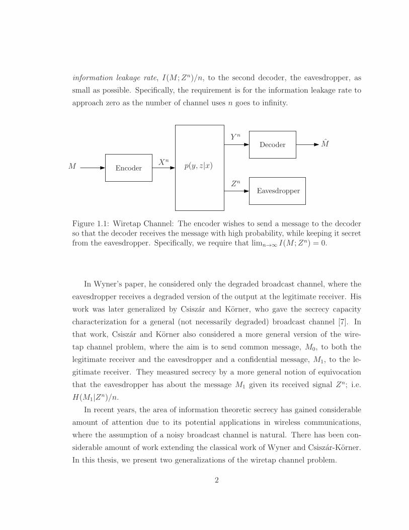
information leakage rate, I(M ;Zn)/n, to the second decoder, the eavesdropper, as
small as possible. Specifically, the requirement is for the information leakage rate to
approach zero as the number of channel uses n goes to infinity.
EncoderM
MDecoder
Eavesdropper
Y n
Zn
p(y, z|x)Xn
Figure 1.1: Wiretap Channel: The encoder wishes to send a message to the decoderso that the decoder receives the message with high probability, while keeping it secretfrom the eavesdropper. Specifically, we require that limn→∞ I(M ;Zn) = 0.
In Wyner’s paper, he considered only the degraded broadcast channel, where the
eavesdropper receives a degraded version of the output at the legitimate receiver. His
work was later generalized by Csiszar and Korner, who gave the secrecy capacity
characterization for a general (not necessarily degraded) broadcast channel [7]. In
that work, Csiszar and Korner also considered a more general version of the wire-
tap channel problem, where the aim is to send common message, M0, to both the
legitimate receiver and the eavesdropper and a confidential message, M1, to the le-
gitimate receiver. They measured secrecy by a more general notion of equivocation
that the eavesdropper has about the message M1 given its received signal Zn; i.e.
H(M1|Zn)/n.
In recent years, the area of information theoretic secrecy has gained considerable
amount of attention due to its potential applications in wireless communications,
where the assumption of a noisy broadcast channel is natural. There has been con-
siderable amount of work extending the classical work of Wyner and Csiszar-Korner.
In this thesis, we present two generalizations of the wiretap channel problem.
2
CHAPTER 1. INTRODUCTION 3
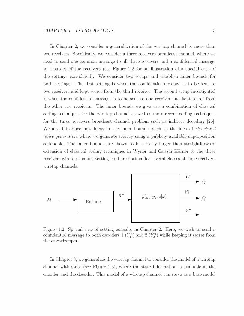
In Chapter 2, we consider a generalization of the wiretap channel to more than
two receivers. Specifically, we consider a three receivers broadcast channel, where we
need to send one common message to all three receivers and a confidential message
to a subset of the receivers (see Figure 1.2 for an illustration of a special case of
the settings considered). We consider two setups and establish inner bounds for
both settings. The first setting is when the confidential message is to be sent to
two receivers and kept secret from the third receiver. The second setup investigated
is when the confidential message is to be sent to one receiver and kept secret from
the other two receivers. The inner bounds we give use a combination of classical
coding techniques for the wiretap channel as well as more recent coding techniques
for the three receivers broadcast channel problem such as indirect decoding [26].
We also introduce new ideas in the inner bounds, such as the idea of structured
noise generation, where we generate secrecy using a publicly available superposition
codebook. The inner bounds are shown to be strictly larger than straightforward
extension of classical coding techniques in Wyner and Csiszar-Korner to the three
receivers wiretap channel setting, and are optimal for several classes of three receivers
wiretap channels.
EncoderMp(y1, y2, z|x)Xn
M
M
Y n1
Y n2
Zn
Figure 1.2: Special case of setting consider in Chapter 2. Here, we wish to send aconfidential message to both decoders 1 (Y n
1 ) and 2 (Y n2 ) while keeping it secret from
the eavesdropper.
In Chapter 3, we generalize the wiretap channel to consider the model of a wiretap
channel with state (see Figure 1.3), where the state information is available at the
encoder and the decoder. This model of a wiretap channel can serve as a base model
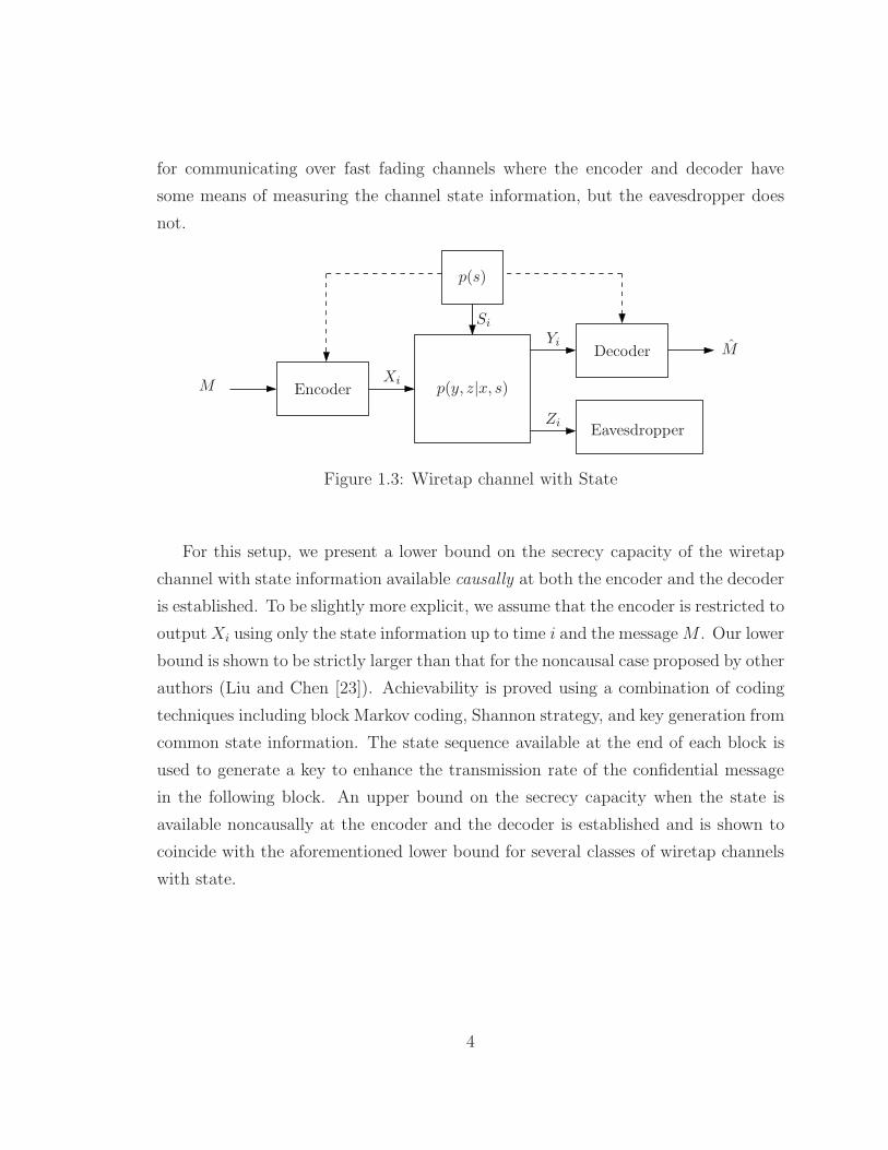
for communicating over fast fading channels where the encoder and decoder have
some means of measuring the channel state information, but the eavesdropper does
not.
MXi
Si
Yi
Zi
M
Encoder
Decoder
Eavesdropper
p(s)
p(y, z|x, s)
Figure 1.3: Wiretap channel with State
For this setup, we present a lower bound on the secrecy capacity of the wiretap
channel with state information available causally at both the encoder and the decoder
is established. To be slightly more explicit, we assume that the encoder is restricted to
outputXi using only the state information up to time i and the messageM . Our lower
bound is shown to be strictly larger than that for the noncausal case proposed by other
authors (Liu and Chen [23]). Achievability is proved using a combination of coding
techniques including block Markov coding, Shannon strategy, and key generation from
common state information. The state sequence available at the end of each block is
used to generate a key to enhance the transmission rate of the confidential message
in the following block. An upper bound on the secrecy capacity when the state is
available noncausally at the encoder and the decoder is established and is shown to
coincide with the aforementioned lower bound for several classes of wiretap channels
with state.
4
CHAPTER 1. INTRODUCTION 5
1.2 Cascade Source Coding
The next area in Network Information Theory that we will be discussing in this
thesis is in the area of multi-terminal source coding, spanning Chapters 4 and 5.
While this is a classical area of research in Network Information Theory, there are
still a number of interesting open problems, both of practical and theoretical interest.
One such problem is the problem of Cascade Source Coding with side information.
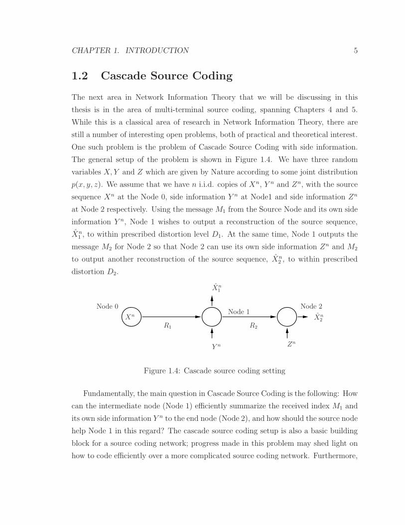
The general setup of the problem is shown in Figure 1.4. We have three random
variables X, Y and Z which are given by Nature according to some joint distribution
p(x, y, z). We assume that we have n i.i.d. copies of Xn, Y n and Zn, with the source
sequence Xn at the Node 0, side information Y n at Node1 and side information Zn
at Node 2 respectively. Using the message M1 from the Source Node and its own side
information Y n, Node 1 wishes to output a reconstruction of the source sequence,
Xn1 , to within prescribed distortion level D1. At the same time, Node 1 outputs the
message M2 for Node 2 so that Node 2 can use its own side information Zn and M2
to output another reconstruction of the source sequence, Xn2 , to within prescribed
distortion D2.
Xn
Y n Zn
R1 R2
Xn1
Xn2
Node 0Node 1
Node 2
Figure 1.4: Cascade source coding setting
Fundamentally, the main question in Cascade Source Coding is the following: How
can the intermediate node (Node 1) efficiently summarize the received index M1 and
its own side information Y n to the end node (Node 2), and how should the source node
help Node 1 in this regard? The cascade source coding setup is also a basic building
block for a source coding network; progress made in this problem may shed light on
how to code efficiently over a more complicated source coding network. Furthermore,
it also has potential practical applications, such as in peer to peer video compression
and transmission over a network, where each node may have side information, such
as previous video frames, about a video to be sent from the source.
When the side informations at Nodes 1 and 2 are absent, the optimum rate-
distortion region can be characterized [39]. When side information is present, this
problem is in general a difficult one. Nevertheless, several interesting partial results
have appeared in recent years characterizing the rate-distortion region under different
settings (see [33], [8], [27], [16], [15], [31]). In Chapter 4, we focus on cases where
the statistical structure on the source and side informations allows us to show the
optimality of some coding schemes. In particular, we consider the Cascade Source
Coding problem, and a generalized version of the Cascade Source Coding problem, the
Triangular Source Coding problem, where the same side information (Y ) is available
at both the source node and Node 1, and the side information available at Node 2
is a degraded version of the side information at the source node and Node 1. We
characterize the rate-distortion region for these problems. For the Cascade setup, we
showed that, at Node 1, decoding and re-binning the codeword sent by the source
node for Node 2 is optimum. We then extend our results to the Two way Cascade
and Triangular setting, where the source node is interested in lossy reconstruction
of the side information at Node 2 via a rate limited link from Node 2 to the source
node. We characterize the rate distortion regions for these settings. Complete explicit
characterizations for all settings are also given in the Quadratic Gaussian case. We
then conclude the chapter with two further extensions: A triangular source coding
problem with a helper, and an extension of our Two Way Cascade setting in the
Quadratic Gaussian case.
In Chapter 5, we consider Cascade and Triangular Source Coding with side in-
formations and causal reconstruction at the end node (Node 2). Here, Node 2 is
constrained to reconstruct the symbol X2i using only the side information from time
1 up to i. This setup of causal source coding (and reconstruction) was first intro-
duced in [34], and motivation for considering this setting can be found in that paper.
Essentially, this problem is motivated by source coding systems that are constrained
to operate with limited or no delay. Source coding systems with encoder and decoder
6

CHAPTER 1. INTRODUCTION 7
delay constraints form a subclass of schemes in the setting proposed by [34], since
their setting only imposes delay restrictions on the decoder. Results and bounds in
that paper therefore serve as bounds on the limits of performance for source coding
systems with delay constraints. Our results in Chapter 5 serve as a partial gener-
alization of the results in that paper to the Cascade and Triangular Source Coding
setting. When the side information at the source and intermediate nodes are the
same, we characterize the rate distortion regions for both the cascade and triangu-
lar source coding problems. The difference between this setting and that found in
Chapter 4 is that the degraded side information assumption is no longer necessary for
characterization of the rate-distortion region. Instead, we impose a causality restric-
tion. We then move on to consider the general cascade setting with causal lossless
reconstruction at the end node. For this setting, we characterize the rate region when
the sources satisfy a positivity condition, or when a Markov chain holds.

Chapter 2
Three receivers broadcast channels
with common and confidential
messages
2.1 Introduction to 3-receivers Wiretap Channel
As mentioned in Chapter 1, the wiretap channel was first introduced in the seminal
paper by Wyner [36]. He considered a 2-receiver broadcast channel where sender X
wishes to communicate a message to receiver Y while keeping it secret from the other
receiver (eavesdropper) Z. Wyner showed that the secrecy capacity when the channel
to the eavesdropper is a degraded version of the channel to the legitimate receiver is
Cs = maxp(x)
(I(X ; Y )− I(X ;Z)).
The main coding idea is to randomly generate 2n(I(X:Y )) xn sequences and partition
them into 2nR message bins, where R < I(X ; Y ) − I(X ;Z). To send a message, a
sequence from the message bin is randomly selected and transmitted. The legitimate
receiver uniquely decodes the codeword and hence the message with high probability,
while the message is kept asymptotically secret from the eavesdropper provided R <
CS.
8

CHAPTER 2. 3 RECEIVERS WIRETAP CHANNEL 9
This result was extended by Csiszar and Korner [7] to general (non-degraded)
2-receiver broadcast channels with common and confidential messages. They estab-
lished the secrecy capacity region, which is the optimal tradeoff between the common
and private message rates and the eavesdropper’s private message equivocation rate.
In the special case of no common message, their result yields the secrecy capacity for
the general wiretap channel,
Cs = maxp(v)p(x|v)
(I(V ; Y )− I(V ;Z)).
The achievability idea is to use Wyner’s wiretap channel coding for the channel from
V to Y by randomly selecting a vn codeword from the message bin and then sending
a random sequence Xn generated according to∏n
i=1 pX|V (xi|vi).
The work in [7] has been extended in several directions by considering different
message demands and secrecy scenarios, e.g., see [22], [3]. However, with some notable
exceptions such as [18] and [10], extending the result of Csiszar and Korner to general
discrete memoryless broadcast channels with more than two receivers has remained
open, since even the capacity region without secrecy constraints for the 3-receiver
broadcast channel with degraded message sets is not known in general. The secrecy
setup for the 3-receiver broadcast channel also has close connections to the compound
wiretap channel model (see [21, Chapter 3] and references therein). Recently, Nair
and El Gamal [26] showed that the straightforward extension of the Korner–Marton
capacity region for the 2-receiver broadcast channel with degraded message sets to
more than 3 receivers is not optimal. They established an achievable rate region for
the general 3-receiver broadcast channel and showed that it can be strictly larger than
the straightforward extension of the Korner–Marton region.
In this chapter, we establish inner and outer bounds on the secrecy capacity region
for the 3-receivers broadcast channel with common and confidential messages. We
consider two setups.
• 2-receiver, 1-eavesdropper : Here the confidential message is to be sent to two
receivers and kept secret from the third receiver (eavesdropper).
• 1-receiver, 2-eavesdroppers : In this setup the confidential message is to be sent
to one receiver and kept secret from the other two receivers.
To illustrate the main coding idea in our new inner bound for the 2-receiver, 1-
eavesdropper setup, consider the special case where a message M ∈ [1 : 2nR] is to be
sent reliably to receivers Y1 and Y2 and kept asymptotically secret from eavesdropper
Z. A straightforward extension of the Csiszar–Korner [7] result for the 2-receiver
wiretap channel yields the lower bound on the secrecy capacity
CS ≥ maxp(v)p(x|v)
min {I(V ; Y1)− I(V ;Z), I(V ; Y2)− I(V ;Z)} . (2.1)
Now, suppose Z is a degraded version of Y1, then from Wyner’s wiretap result, we
know that (I(V ; Y1) − I(V ;Z)) ≤ (I(X ; Y1) − I(X ;Z)) for all p(v, x). However, no
such inequality holds in general for the second term under the minimum. As a special
case of the inner bound in Theorem 2.1, we show that the rate obtained by replacing
V by X only in the first term in (2.1) is achievable, that is, we establish the lower
bound
CS ≥ maxp(v)p(x|v)
min {I(X ; Y1)− I(X ;Z), I(V ; Y2)− I(V ;Z)} . (2.2)
To prove achievability of (2.2), we again randomly generate 2n(I(V ;Y2)−δ) vn sequences
and partition them into 2nR bins, where R = (I(V ; Y2) − I(V ;Z)). For each vn
sequence, we randomly and conditionally independently generate 2nI(X;Z|V ) xn se-
quences. The vn and xn sequences are revealed to all parties, including the eaves-
dropper. To send a message m, the encoder randomly chooses a vn sequence from bin
m. It then randomly chooses an xn sequence from the codebook for the selected vn
sequence (instead of randomly generating an Xn sequence as in the Csiszar–Korner
scheme) and transmits it. Receiver Y2 decodes vn directly, while receiver Y1 decodes v
n
indirectly through xn [26]. In Section 2.3, we show through an example that this new
lower bound can be strictly larger than the extended Csiszar–Korner lower bound.
We then show in Theorem 2.1 that this lower bound can be generalized further via
Marton coding.
The rest of the chapter is organized as follows. In the next section we present
10
CHAPTER 2. 3 RECEIVERS WIRETAP CHANNEL 11
needed definitions. In Section 2.3, we provide an alternative proof of achievability for
the Csiszar–Korner 2-receiver wiretap channel that uses superposition coding and ran-
dom codeword selection instead of random generation of the transmitted codeword.
This technique is used in subsequent sections to establish the new inner bounds for
the 3-receiver setups. In Section 2.4, we present the inner bound for the 2-receiver, 1-
eavesdropper case. We show that this inner bound is tight for the reversely degraded
product broadcast channel and when the eavesdropper is less noisy than both legiti-
mate receivers. In Section 2.5, we present inner and outer bounds for the 1-receiver,
2-eavesdropper setup for 3-receiver multilevel broadcast channel [4]. We show that
the bounds coincide in several special cases.
2.2 Definitions and Problem Setup
Consider a 3-receiver discrete memoryless broadcast channel with input alphabet X ,
output alphabets Y1,Y2,Y3 and conditional pmfs p(y1, y2, y3|x). We investigate the
following two setups.
2.2.1 2-Receivers, 1-Eavesdropper
Here the confidential message is to be sent to receivers Y1 and Y2 and is to be kept
secret from the eavesdropper Y3 = Z). A (2nR0, 2nR1, n) code for this scenario consists
of: (i) two messages (M0,M1) uniformly distributed over [1 : 2nR0 ]× [1 : 2nR1]; (ii) an
encoder that randomly generates a codeword Xn(m0, m1) according to the conditional
pmf p(xn|m0, m1); and (iii) 3 decoders; the first decoder assigns to each received
sequence yn1 an estimate (M01, M11) ∈ [1 : 2nR0] × [1 : 2nR1] or an error message, the
second decoder assigns to each received sequence yn2 an estimate (M02, M12) ∈ [1 :
2nR0]× [1 : 2nR1] or an error message, and the third decoder assigns to each received
sequence zn an estimate M03 ∈ [1 : 2nR0 ] or an error message. The probability of
error for this scenario is defined as
P(n)e1 = P
{
M0j 6= M0 for j = 1, 2, 3 or M1j 6= M1for j = 1, 2}
.
The equivocation rate at receiver Z, which measures the amount of uncertainty re-
ceiver Z has about message M1, is defined as H(M1|Zn)/n.
A secrecy rate tuple (R0, R1, Re) is said to be achievable if
limn→∞
P(n)e1 = 0, and
lim infn→∞
1
nH(M1|Z
n) ≥ Re.
The secrecy capacity region is the closure of the set of achievable rate tuples
(R0, R1, Re).
For this setup, we also consider the special case of asymptotic perfect secrecy, where
no common message is to be sent to Z and a confidential message, M ∈ [1 : 2nR], is
to be sent to Y1 and Y2 only. The probability of error is as defined above with R0 = 0
and R1 = R. A secrecy rate R is said to be achievable if there exists a sequence of
(2nR, n) codes such that
limn→∞
P(n)e1 = 0, and
lim infn→∞
1
nH(M |Zn) ≥ R.
The secrecy capacity, CS, is the supremum of all achievable rates.
2.2.2 1-Receiver, 2-Eavesdroppers
In this setup, the confidential message is to be sent to receiver Y1 and kept secret
from eavesdroppers Y2 = Z2 and Y3 = Z3. A (2nR0 , 2nR1, n) code consists of the
same message sets and encoding function as in the 2-receiver, 1-eavesdropper case.
The first decoder assigns to each received sequence yn1 an estimate (M01, M1) ∈ [1 :
2nR0] × [1 : 2nR1 ] or an error message, the second decoder assigns to each received
sequence zn2 an estimate M02 ∈ [1 : 2nR0] or an error message, and the third decoder
assigns to each received sequence zn3 an estimate M03 ∈ [1 : 2nR0] or an error message.
12
CHAPTER 2. 3 RECEIVERS WIRETAP CHANNEL 13
The probability of error is
P(n)e2 = P{M0j 6= M0for j = 1, 2, 3or M1 6= M1}.
The equivocation rates at the two eavesdroppers are H(M1|Zn2 )/n and H(M1|Z
n3 )/n,
respectively.
A secrecy rate tuple (R0, R1, Re2, Re3) is said to be achievable if
limn→∞
P(n)e2 = 0,
lim infn→∞
1
nH(M1|Z
nj ) ≥ Rej , j = 2, 3.
The secrecy capacity region is the closure of the set of achievable rate tuples (R0, R1, Re2, Re3).
For simplicity of presentation, we consider only the special class of multilevel broad-
cast channels [4].
2.3 2-receiver wiretap channel
We first revisit the 2-receiver wiretap channel, where a confidential message is to
be sent to the legitimate receiver Y and kept secret from the eavesdropper Z. The
secrecy capacity for this case is a special case of the secrecy capacity region for the
broadcast channel with common and confidential messages established in [7].
Proposition 2.1. The secrecy capacity of the 2-receiver wiretap channel is
CS = maxp(v,x)
(I(V ; Y )− I(V ;Z)).
In the following, we provide a new proof of achievability for this result in which
the second randomization step in the original proof is replaced by a random codeword
selection from a public superposition codebook. As we will see, this proof technique
allows us to use indirect decoding to establish new inner bounds for the 3-receiver
wiretap channels.
Proof of Achievability for Proposition 2.1:
Fix p(v, x). Randomly and independently generate sequences vn(l0), l0 ∈ [1 : 2nR],
each according to∏n
i=1 pV (vi). Partition the set [1 : 2nR] into 2nR bins B(m) =
[(m − 1)2n(R−R) + 1 : m2n(R−R)], m ∈ [1 : 2nR]. For each l0 ∈ [1 : 2nR], randomly
and conditionally independently generate sequences xn(l0, l1), l1 ∈ [1 : 2nR1 ], each
according to∏n
i=1 pX|V (xi|vi). The codebook {(vn(l0), xn(l0, l1))} is revealed to all
parties. To send the message m, an index L0 ∈ B(m) is selected uniformly at random
(as in Wyner’s original proof). The encoder then randomly and independently selects
an index L1 and transmits xn(L0, L1). Receiver Y decodes L0 by finding the unique
index l0 such that (vn(l0), yn) ∈ T
(n)ǫ . By the law of large numbers and the packing
lemma [13, Chapter 3], the average probability of error approaches zero as n → ∞ if
R < (V ; Y )− δ(ǫ).
We now show that I(M ;Zn|C) ≤ nδ(ǫ). Considering the mutual information
between Zn and M , averaged over the random codebook C, we have
I(M ;Zn|C) = I(M,L0, L1;Zn|C)− I(L0, L1;Z
n|M, C)
(a)
≤ I(Xn;Zn|C)−H(L0, L1|M, C) +H(L0, L1|M,Zn, C)
≤n∑
i=1
I(Xi;Zi|C)− n(R− R)− nR1 +H(L0, L1|M,Zn, C)
≤ nI(X ;Z)− n(R + R1 − R) +H(L0|M,Zn, C) +H(L1|L0, Zn, C).
(2.3)
(a) follows since (M,L0, L1, C) → Xn → Zn from the discrete memoryless property
of the channel. The last step follows from follows since H(Zi|C) ≤ H(Zi) = H(Z)
and H(Zi|Xi, C) =∑
C p(C)p(xi|C)H(Z|xi, C) =∑
C p(C)p(vi|C)H(Z|xi) = H(Z|X)
It remains to upper bound H(L0|M,Zn, C) and H(L1|L0, Zn, C). By symmetry of
14
CHAPTER 2. 3 RECEIVERS WIRETAP CHANNEL 15
codebook construction, we have
H(L0|M,Zn, C) = 2−nR
2nR∑
m=1
H(L0|M = m,Zn, C)
= H(L0|Zn,M = 1, C),
H(L1|L0, Zn, C) = 2−nR
∑
l0
H(L1|L0 = l0, Zn, C)
= H(L1|L0 = 1, vn(1), Zn, C).
To further bound these terms, we use the following key lemma.
Lemma 2.1. Let (U, V, Z) ∼ p(u, v, z), S ≥ 0 and ǫ > 0. Let Un be a random
sequence distributed according to∏n
i=1 pU(ui). Let V n(l), l ∈ [1 : 2nS], be a set of
random sequences that are conditionally independent given Un and each distributed
according to∏n
i=1 pV |U(vi|ui), and let C = {Un, V n(1), V n(2), . . . V n(2nS)}. Let L ∈
[1 : 2nS] be a random index with an arbitrary probability mass function. Then, if
P{(Un, V n(L), Zn) ∈ T(n)ǫ } → 1 as n → ∞ and S > I(V ;Z|U) + δ(ǫ), there exists a
δ′(ǫ) > 0, where δ′(ǫ) → 0 as ǫ → 0, such that, for n sufficiently large,
H(L|Zn, Un, C) ≤ n(S − I(V ;Z|U)) + nδ′(ǫ).
The proof of this lemma is given in Appendix A.1. An illustration of the random
sequence structure is given in Figure 2.1.
Now, returning to (2.3), we note that P{(V n(L0), Xn(L0, L1), Z
n) ∈ T(n)ǫ } → 1 as
n → ∞ by law of large numbers. Hence, we can apply Lemma 2.1 to obtain
H(L0|Zn,M = 1, C) ≤ n(R− R)− nI(V ;Z) + nδ(ǫ), (2.4)
H(L1|L0 = 1, V n, Zn, C) ≤ n(R1 − I(X ;Z|V )) + nδ(ǫ), (2.5)
if R−R > I(V ;Z) + δ(ǫ) and R1 > I(X ;Z|V ) + δ(ǫ). Substituting from inequalities
(2.4) and (2.5) into (2.3) shows that I(M ;Zn|C) ≤ 2nδ(ǫ). We then recover the
original asymptotic secrecy rate by noting that the constraint of R1 > I(X ;Z|V )+δ(ǫ)
Un
Zn
V n(1) V n(2) V n(2nS)V n(L)
Figure 2.1: Structure of random sequences in Lemma 2.1. V n(l) is generated ac-cording to
∏ni=1 pV |U(vi|ui). Solid arrows represent the sequence pair (Un, V n(L), Zn)
while the dotted arrows to Zn represent the other V n sequences jointly typical withthe (Un, Zn) pair. Lemma 2.1 gives an upper bound on the number of V n sequencesthat can be jointly typical with a (Un, Zn) pair.
is not tight. This completes the proof of Proposition 2.1.
Remark 2.3.1. In the proof of Proposition 2.1 in [7], the encoder transmits a ran-
domly generated codeword Xn ∼∏n
i=1 pX|V (xi|vi). Although replacing random Xn
generation by superposition coding and random codeword selection in our alternative
proof does not increase the achievable secrecy rate for the 2-receiver wiretap channel,
it can increase the rate when there are more than one legitimate receiver, as we show
in the next sections.
2.4 2-receivers, 1-eavesdropper wiretap channel
We establish an inner bound on the secrecy capacity for the 3-receiver wiretap channel
with one common and one confidential message when the confidential message is to
be sent to receivers Y1 and Y2 and kept secret from receiver Z. In the following
subsection, we consider the case where M0 = ∅ and M1 = M ∈ [1 : 2nR] is to be
kept asymptotically secret from Z. This result is then extended in Subsection 2.4.2
to establish an inner bound on the secrecy capacity region.
16

CHAPTER 2. 3 RECEIVERS WIRETAP CHANNEL 17
2.4.1 Asymptotic perfect secrecy
We establish the following lower bound on secrecy capacity for the case where a
confidential message is to be sent to receivers Y1 and Y2 and kept secret from the
eavesdropper Z.
Theorem 2.1. The secrecy capacity of the 2-receiver, 1-eavesdropper setup with one
confidential message and asymptotic secrecy is lower bounded as follows
CS ≥ min {I(V0, V1; Y1|Q)− I(V0, V1;Z|Q), I(V0, V2; Y2|Q)− I(V0, V2;Z|Q)}
for some p(q, v0, v1, v2, x) = p(q, v0)p(v1, v2|v0)p(x|v1, v2, v0) such that I(V1, V2;Z|V0) ≤
I(V1;Z|V0) + I(V2;Z|V0)− I(V1;V2|V0).
In addition to superposition coding and the new coding idea discussed in the
previous section, Theorem 2.1 also uses Marton coding [24].
For clarity, we first establish the following Corollary.
Corollary 2.1. The secrecy capacity for the 2-receiver, 1-eavesdropper with one con-
fidential message and asymptotic secrecy is lower bounded as follows
CS ≥ maxp(q)p(v|q)p(x|v)
min {I(X ; Y1|Q)− I(X ;Z|Q), I(V ; Y2|Q)− I(V ;Z|Q)} .
Remark 2.4.1. Consider the case where X → Y1 → Z form a Markov chain. Then,
we can show that Theorem 2.1 reduces to Corollary 2.1, i.e., the achievable secrecy
rate is not increased by using Marton coding when X → Y1 → Z (or X → Y2 → Z by
symmetry) form a Markov chain. To see this, note that (I(X ; Y1|Q)− I(X ;Z|Q)) ≥
(I(V1, V0; Y1|Q) − I(V1, V0;Z|Q)) for all V1 if X → Y1 → Z. Next, note that we can
set V = (V0, V2) in Corollary 2.1 to obtain the rate in Theorem 2.1.
Proof of Corollary 2.1:
Codebook generation
Randomly and independently generate the time-sharing sequence qn according to∏n
i=1 pQ(qi). Next, randomly and conditionally independently generate 2nR sequences
vn(l0), l0 ∈ [1 : 2nR], each according to∏n
i=1 pV |Q(vi|qi). Partition the set [1 : 2nR]
into 2nR equal size bins B(m), m ∈ [1 : 2nR]. For each l0, conditionally independently
generate sequences xn(l0, l1), l1 ∈ [1 : 2nR1], each according to∏n
i=1 pX|V (xi|vi).
Encoding
To send a message m ∈ [1 : 2nR], randomly and independently choose an index
L0 ∈ C(m) and an index L1 ∈ [1 : 2nR1 ], and send xn(L0, L1).
Decoding
Assume without loss of generality that L0 = 1 and m = 1. Receiver Y2 finds L0, and
hence m, via joint typicality decoding. By the law of large number and the packing
lemma, the probability of error approaches zero as n → ∞ if
R < I(V ; Y2|Q)− δ(ǫ).
Receiver Y1 finds L0 (and hence m) via indirect decoding. That is, it declares
that L0 is sent if it is the unique index such that (qn, vn(L0), xn(L0, l1), Y
n1 ) ∈ T
(n)ǫ
for some l1 ∈ [1 : 2nR1 ]. To analyze the average probability of error P(E), define the
error events
E10 = {(Qn, Xn(1, 1), Y n1 ) /∈ T (n)
ǫ },
E11 = {(Qn, Xn(l0, l1), Yn1 ) ∈ T (n)
ǫ for some l0 6= 1}.
Then, by union of events bound the probability of error is upper bounded as
P(E) ≤ P{E10}+ P{E11}.
18
CHAPTER 2. 3 RECEIVERS WIRETAP CHANNEL 19
Now by law of large numbers, P{E10} → 0 as n → ∞. Next consider
P{E11} ≤∑
l0 6=1
∑
l1
P
{
(Qn, V n(l0), Xn(l0, l1), Y
n1 )
∈ T(n)ǫ
}
≤∑
l0 6=1
∑
l1
2−n(I(V,X;Y1|Q)−δ(ǫ))
≤ 2n(R+R1−I(V,X;Y1|Q)+δ(ǫ)).
Hence, P{E11} → 0 as n → ∞ if
R + R1 < I(X ; Y1|Q)− δ(ǫ).
Analysis of equivocation rate
To bound the equivocation rate term H(M |Zn, C), we proceed as before and show
that the I(M ;Zn|C) ≤ 2nδ(ǫ). Note that the only difference between this case and
the analysis for the 2-receiver case in Section 2.2 is the addition of the time-sharing
random variable Q. Since
P{(Qn, V n(L0), Xn(L0, L1), Z
n) ∈ T(n)ǫ } → 1 as n → ∞, we can apply Lemma 2.1
(with the addition of the time sharing random variable). Following the analysis in
Section 2.2, it is easy to see that I(M ;Zn|C) ≤ 2nδ(ǫ) if
R− R > I(V ;Z|Q) + δ(ǫ),
R1 > I(X ;Z|V ) + δ(ǫ).
Finally, using Fourier–Motzkin elimination on the set of inequalities completes the
proof of achievability.
Before proving Theorem 2.1, we show through an example that the lower bound
in Corollary 2.1 can be strictly larger than the rate of the straightforward extension
of the Csiszar–Korner scheme to the 2-receiver, 1-eavesdropper setting,
RCK = maxp(q)p(v|q)p(x|v)
min {I(V ; Y1|Q)− I(V ;Z|Q), I(V ; Y2|Q)− I(V ;Z|Q)} . (2.6)
Note that Theorem 2.1 includes RCK as a special case (through setting V0 = V1 =
V2 = V in Theorem 2.1).
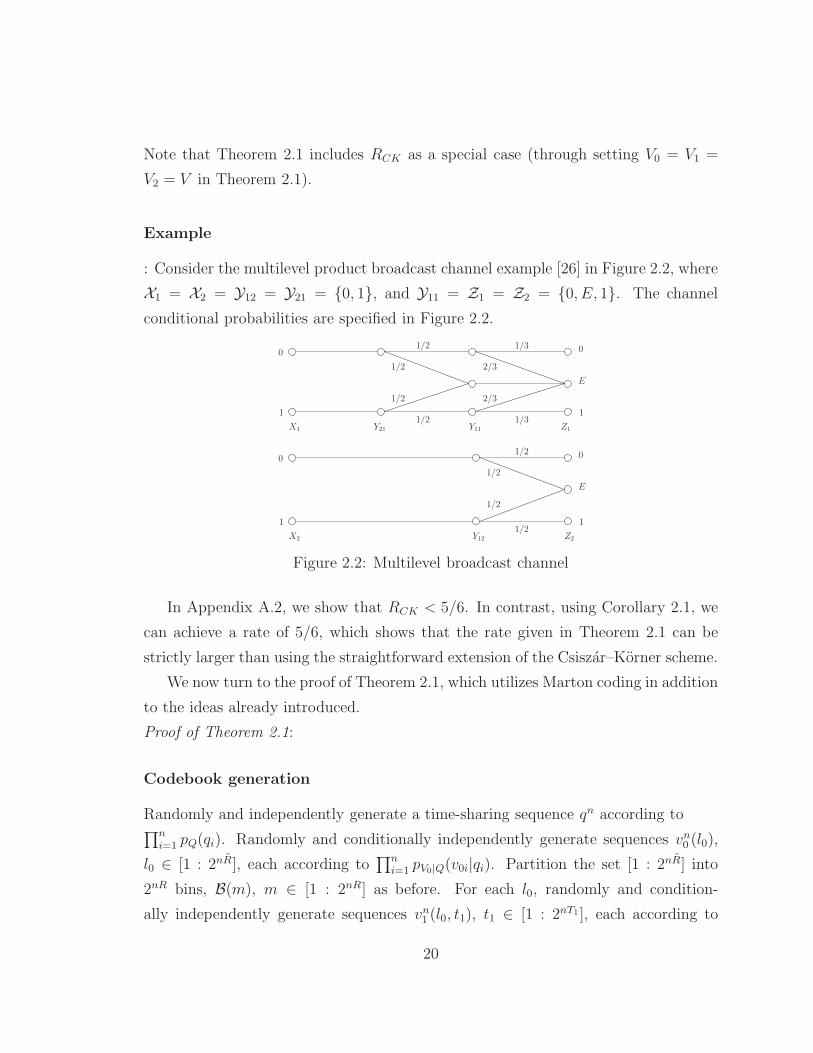
Example
: Consider the multilevel product broadcast channel example [26] in Figure 2.2, where
X1 = X2 = Y12 = Y21 = {0, 1}, and Y11 = Z1 = Z2 = {0, E, 1}. The channel
conditional probabilities are specified in Figure 2.2.
1/2
1/2
1/3
1/3
1/2
1/2
2/3
2/3
1/2
1/2
1/2
1/2
0
00
0
1
1
1
1
E
E
Y21 Y11
Y12 Z2
Z1X1
X2
Figure 2.2: Multilevel broadcast channel
In Appendix A.2, we show that RCK < 5/6. In contrast, using Corollary 2.1, we
can achieve a rate of 5/6, which shows that the rate given in Theorem 2.1 can be
strictly larger than using the straightforward extension of the Csiszar–Korner scheme.
We now turn to the proof of Theorem 2.1, which utilizes Marton coding in addition
to the ideas already introduced.
Proof of Theorem 2.1:
Codebook generation
Randomly and independently generate a time-sharing sequence qn according to∏n
i=1 pQ(qi). Randomly and conditionally independently generate sequences vn0 (l0),
l0 ∈ [1 : 2nR], each according to∏n
i=1 pV0|Q(v0i|qi). Partition the set [1 : 2nR] into
2nR bins, B(m), m ∈ [1 : 2nR] as before. For each l0, randomly and condition-
ally independently generate sequences vn1 (l0, t1), t1 ∈ [1 : 2nT1 ], each according to
20
CHAPTER 2. 3 RECEIVERS WIRETAP CHANNEL 21
∏ni=1 pV1|V0(v1i|v0i). Partition the set [1 : 2nT1 ] into 2nR1 equal size bins, B(l0, l1).
Similarly, for each l0, generate sequences vn2 (l0, t2), t2 ∈ [1 : 2nT2], each according to∏n
i=1 pV2|V0(v2i|v0i), and partition [1 : 2nT1] into 2nR2 equal size bins, B(l0, l2).
Encoding
To send message m, the encoder first randomly chooses an index L0 ∈ B(m). It then
randomly chooses a product bin indices (L1, L2) and selects a jointly typical sequence
pair (vn1 (L0, t1(L0, L1)), vn2 (L0, t2(L0, L2)) in the product bin. If there is more than
one such pair, pick one of them uniformly at random. An error event occurs if no
such pair is found, in which case, the encoder picks the indices t1 ∈ B(L0, L1) and
t2 ∈ B(L0, L2) uniformly at random. This encoding step succeeds with probability of
error that approaches zero as n → ∞, if [14]
R1 + R2 < T1 + T2 − I(V1;V2|V0)− δ(ǫ).
Finally, the encoder generates a codeword Xn at random according to∏n
i=1 pX|V0,V1,V2(xi|v0i, v1i, v2i) and transmits it.
Decoding and analysis of the probability of error
Receiver Y1 decodes L0 and hencem indirectly by finding the unique index l0 such that
(vn0 (l0), vn1 (l0, t1), y
n1 ) ∈ T
(n)ǫ for some t1 ∈ [1 : 2nT1]. Similarly, receiver Y2 finds L0
(and hence m) indirectly by finding the unique index l0 such that (vn0 (l0), vn2 (l0, T2)) ∈
T(n)ǫ for some l2 ∈ [1 : 2nT2]. Following the analysis given earlier, it is easy to see that
these steps succeed with probability of error that approaches zero as n → ∞ if
R + T1 < I(V0, V1; Y1|Q)− δ(ǫ),
R + T2 < I(V0, V1; Y2|Q)− δ(ǫ).
Analysis of equivocation rate
A codebook C induces a joint pmf on (M,L0, L1, L2, Vn0 , V
n1 , V
n2 , Z
n) of the form
p(m, l0, l1, l2, vn0 , v
n1 , v
n2 z
n|c) = 2−n(R+R1+R2)p(vn0 , vn1 , v
n2 |l0, l1, l2, c).
∏ni=1 pZ|V0,V1,V2
(zi|v0i, v1i, v2i). We again analyze the mutual information between M
and (Zn, Qn), averaged over codebooks.
I(M ;Zn, Qn|C) = I(M ;Zn|Qn, C)
= I(T1(L0, L1), T2(L0, L1), L0,M ;Zn|Qn, C)
− I(T1(L0, L1), T2(L0, L2), L0;Zn|M,Qn, C)
≤ I(V n0 , V
n1 , V
n2 ;Z
n|Qn, C)− I(L0;Zn|M,Qn, C)
− I(T1(L0, L1), T2(L0, L2);Zn|L0, Q
n, C)
≤ nI(V0, V1, V2;Z|Q)−H(L0|M,Qn, C) +H(L0|M,Qn, Zn, C)
− I(T1(L0, L1), T2(L0, L2);Zn|L0, Q
n, C) + nδ(ǫ). (2.7)
In the last step, we bound the term I(V n0 , V
n1 , V
n2 ;Z
n|Qn, C) by the following argu-
ment, which is an extension of a similar argument in [36]. For simplicity of notation,
let V = (V0, V1, V2). We wish to show that I(V n;Zn|Qn, C) ≤ nI(V ;Z)+nδ(ǫ). Note
that X is generated according to p(xi|vi). Define E = 1 if (qn, vn, zn) are not jointly
typical and 0 otherwise, and N(v) = |{Vi : Vi = v}|. Then,
I(V n;Zn|C, Qn) ≤ 1 + P(E = 0)I(V ;Zn|C, E = 0, Qn)
+ P(E = 1)I(V ;Zn|C, E = 1, Qn)
≤ 1 + P(E = 0)I(V ;Zn|C, E = 0, Qn)
+ P(E = 1)n log |Z| − P(E = 1)H(Zn|C, V n, Qn, E = 1)
= 1 + P(E = 0)(H(Zn|C, E = 0, Qn)−H(Zn|C, V n, Qn)
+ P(E = 1)n log |Z|.
22
CHAPTER 2. 3 RECEIVERS WIRETAP CHANNEL 23
Note that H(Zn|C, E = 0, Qn) ≤ nH(Z|Q) + nδ(ǫ). For H(Zn|C, V n, Qn, E = 0) =
H(Zn|C, V n, E = 0), we have
H(Zn|C, E = 0, V n) ≥∑
c,vn∈T(n)ǫ
P(V n = vn, C = c)H(Zn|C = c, V n = vn)
=∑
c,vn∈T(n)ǫ
P(V n = vn, C = c).
(
n∑
i=1
H(Zi|C = c, V n = vn, Z i−1)
)
(a)=
∑
c,vn∈T(n)ǫ
P(V n = vn, C = c)
n∑
i=1
H(Zi|Vi = vi)
=∑
c,vn∈T(n)ǫ
P(V n = vn, C = c)∑
v∈V
N(v)H(Z|V = v)
(b)
≥∑
c,vn∈T(n)ǫ
P(V n = vn, C = c).
(
∑
v∈V
n(p(v)− δ(ǫ))H(Z|V = v)
)
≥ nH(Z|V )− nδ′(ǫ),
where (a) follows since given Vi, Xi is generated randomly according to p(xi|vi) and
since the channel is memoryless, Zi is independent of all other random variables, and
(b) follows since vn is typical, which implies that N(v) ≥ np(v)−nδ(ǫ). Finally, since
the coding scheme satisfies the encoding constraints, the proof is completed by noting
that P(E = 1) → 0 as n → ∞ by the law of large numbers and the mutual covering
lemma in [13, Chapter 9]).
We now bound each remaining terms in inequality (2.7) separately. Note that
H(L0|M,Qn, C) = n(R −R), (2.8)
H(L0|M,Qn, Zn, C)(a)
≤ n(S0 − R− I(V0;Z|Q)) + nδ(ǫ), (2.9)
where (a) follows by similar steps to the proof of Corollary 2.1 and application of
Lemma 2.1, which holds if P{(Qn, V n0 (L0), Z
n) ∈ T(n)ǫ } → 1 as n → ∞ and S0−R ≥
I(V0;Z|Q) + δ(ǫ). The first condition follows since
P
{
(
Qn, V n0 (L0), V
n1 (L0, T1(L0, L1)), V
n2 (L0, T2(L0, L2)), Z
n)
∈ T (n)ǫ
}
→ 1
as n → ∞. Next, consider
I(T1(L0, L1), T2(L0, L2);Zn|L0, Q
n, C)
= H(T1(L0, L1), T2(L0, L2)|L0, Qn, C)−H(T1(L0, L1), T2(L0, L2)|L0, Q
n, Zn, C)
(a)= H(T1(L0, L1), T2(L0, L2), L1, L2|L0, Q
n, C)
−H(T1(L0, L1), T2(L0, L2)|L0, Qn, Zn, C)
≥ H(L1, L2|L0, Qn, C)−H(T1(L0, L1)|L0, Q
n, Zn, C)
−H(T2(L0, L2)|L0, Qn, Zn, C), (2.10)
where (a) holds since given the codebook C and L0, (L1, L2) is a deterministic function
of (T1(L0, L1), T2(L0, L2)). Now,
H(L1, L2|L0, Qn, C) = n(R1 + R2), (2.11)
H(T1(L0, L1)|L0, Qn, Zn, C)
(b)
≤ n(T1 − I(V1;Z|V0) + δ(ǫ)), (2.12)
H(T2(L0, L2)|L0, Qn, Zn, C)
(c)
≤ n(T2 − I(V2;Z|V0) + δ(ǫ)), (2.13)
where (b) and (c) come from the following analysis. First consider
H(T1(L0, L1)|L0, Qn, Zn, C) = H(T1(L0, L1)|v
n0 (L0), Q
n, Zn, L0, C)
≤ H(T1(L0, L1)|Vn0 , Z
n, C).
We now upper bound the term H(T1(L0, L1)|Vn0 , Z
n, C).
Since
P
{
(
Qn, V n0 (L0), V
n1 (L0, T1(L0, L1)), V
n2 (L0, T2(L0, L2)), Z
n)
∈ T (n)ǫ
}
→ 1
24
CHAPTER 2. 3 RECEIVERS WIRETAP CHANNEL 25
as n → ∞, P{(V n0 (L0), V
n1 (L0, T1(L0, L1)), Z
n) ∈ T(n)ǫ } → 1 as n → ∞. We can
therefore apply Lemma 1 to obtain
H(T1(L0, L1)|L0, Qn, Zn, C) ≤ n(T1 − I(V1;Z|V0))
+ nδ(ǫ),
if T1 > I(V1;Z|V0) + δ(ǫ).
The term H(T2(L0, L2)(L0, L2)|L0, Qn, Zn, C) can be bound using the same steps
to give
H(T2(L0, L2)|L0, Qn, Zn, C) ≤ n(T2 − I(V2;Z|V0)) + nδ(ǫ),
if T2 > I(V2;Z|V0) + δ(ǫ).
Substituting from (2.11), (2.12), and (2.13) into (2.10) yields
I(T1(L0, L1), T2(L0, L2);Zn|L0, Q
n, C) ≥ n(R1 + R2)− n(T1 − I(V1;Z|V0) + δ(ǫ))
− n(T2 − I(V2;Z|V0) + δ(ǫ)). (2.14)
Substituting inequality (2.14), together with (2.8) and (2.9) into (2.7) then yields
I(M ;Zn|Qn, C) ≤ n(I(V1, V2;Z|V0) + T1 + T2 − R1 − R2)
− n(I(V1;Z|V0)− I(V2;Z|V0) + 3δ(ǫ)).
Hence, I(M ;Zn|Qn, C) ≤ 6nδ(ǫ) if
I(V1, V2;Z|V0) + T1 + T2 − R1 − R2 − I(V1;Z|V0)− I(V2;Z|V0) ≤ 3nδ(ǫ).
In summary, the rate constraints arising from analysis of equivocation are
S0 − R > I(V0;Z|Q),
T1 > I(V1;Z|V0),
T2 > I(V2;Z|V0),
T1 + T2 − R1 − R2 ≤ I(V1;Z|V0) + I(V2;Z|V0)− I(V1, V2;Z|V0).
Applying Fourier-Motzkin elimination gives
R < I(V0, V1; Y1|Q)− I(V0, V1;Z|Q),
R < I(V0, V2; Y2|Q)− I(V0, V2;Z|Q),
2R < I(V0, V1; Y1|Q) + I(V0, V2; Y2|Q)− 2I(V0;Z|Q)− I(V1;V2|V0)
for some p(q, v0, v1, v2, x) = p(q, v0)p(v1, v2|v0)p(x|v1, v2, v0) such that I(V1, V2;Z|V0) ≤
I(V1;Z|V0) + I(V2;Z|V0)− I(V1;V2|V0).
The proof of Theorem 2.1 is then completed by observing that the third inequality
is redundant. This is seen by summing the first two inequalities to yield
2R ≤ I(V0, V1; Y1|Q)− I(V0, V1;Z|Q) + I(V0, V2; Y2|Q)− I(V0, V2;Z|Q)
= I(V0, V1; Y1|Q)− I(V0, V1;Z|Q) + I(V0, V2; Y2|Q)
− 2I(V0;Z|Q)− I(V1;Z|V0)− I(V2;Z|V0).
This inequality is at least as tight as the third inequality because of the constraint
on the pmf. This completes the proof of Theorem 2.1.
Special Cases:
We consider several special cases in which the inner bound in Theorem 2.1 is tight.
26
CHAPTER 2. 3 RECEIVERS WIRETAP CHANNEL 27
Reversely Degraded Product Broadcast Channel
As an example of Theorem 2.1, consider the reversely degraded product broadcast
channel with sender X = (X1, X2 . . . , Xk), receivers Yj = (Yj1, Yj2 . . . , Yjk) for j =
1, 2, 3, and conditional probability mass functions p(y1, y2, z|x) =∏k
l=1 p(y1l, y2l, zl|xl).
In [18], the following lower bound on secrecy capacity is established
CS ≥ minj∈{1,2}
k∑
l=1
[I(Ul; Yjl)− I(Ul;Zl)]+. (2.15)
for some p(u1, . . . , uk, x) =∏k
l=1 p(ul)p(xl|ul). Furthermore, this lower bound is
shown to be optimal when the channel is reversely degraded (with Ul = Xl), i.e.,
when each sub-channel is degraded but not necessarily in the same order. We can
show that this result is a special case of Theorem 2.1. Define the sets of l in-
dexes: C = {l : I(Ul; Y1l) − I(Ul;Zl) ≥ 0, I(Ul; Y2l) − I(Ul;Zl) ≥ 0}, A = {l :
I(Ul; Y1l) − I(Ul;Zl) ≥ 0} and B = {l : I(Ul; Y2l) − I(Ul;Zl) ≥ 0}. Now, setting
V0 = {Ul : l ∈ C}, V1 = {Ul : l ∈ A}, and V2 = {Ul : l ∈ B} in the rate expression
of Theorem 2.1 yields (2.15). Note that the constraint in Theorem 2.1 is satisfied for
this choice of auxiliary random variables. The expanded equations are as follows:
I(V1, V2;Z|V0) = I(UA, UB;Z|UC)
= I(UA\C , UB\C ;Z\C)
= I(UA\C ;Z,A\C) + I(UB\C ;Z,B\C)
= I(V1;Z|V0) + I(V2;Z|V0),
I(V0, V1; Y1)− I(V0, V1;Z) = I(UA; Y1,A)− I(UA;ZA),
I(V0, V1; Y1)− I(V0, V1;Z) = I(UB; Y1,A)− I(UB;ZB),
I(V1;V2|V0) = I(UA\C ;UB\C) = 0.

Receivers Y1 and Y2 are less noisy than Z
Recall that in a 2-receiver broadcast channel, a receiver Y is said to be less noisy [20]
than a receiver Z if I(U ; Y ) ≥ I(U ;Z) for all p(u, x). In this case, we have
CS = maxp(x)
min {I(X ; Y1)− I(X ;Z), I(X ; Y2)− I(X ;Z)} .
To show achievability, we set Q = ∅ and V0 = V1 = V2 = V3 = X in Theorem 2.1. The
converse follows similar steps to the converse for Proposition 2.2 in Subsection 2.4.2
given in Appendix A.4 and we omit it here.
2.4.2 2-Receivers, 1-Eavesdropper with Common Message
As a generalization of Theorem 2.1, consider the setting with both common and
confidential messages, where we are interested in achieving some equivocation rate
for the confidential message rather than asymptotic secrecy. For this setting we can
establish the following inner bound on the secrecy capacity region.
Theorem 2.2. An inner bound to the secrecy capacity region of the 2-receiver, 1-
eavesdropper broadcast channel with one common and one confidential messages is
given by the set of rate tuples (R0, R1, Re) such that
R0 < I(U ;Z),
R0 +R1 < I(U ;Z) + min {I(V0, V1; Y1|U)− I(V1;Z|V0),
I(V0, V2; Y2|U)− I(V2;Z|V0)} ,
R0 +R1 < min {I(V0, V1; Y1)− I(V1;Z|V0), I(V0, V2; Y2)− I(V2;Z|V0)} ,
Re ≤ R1,
Re < min {I(V0, V1; Y1|U)− I(V0, V1;Z|U), I(V0, V2; Y2|U)− I(V0, V2;Z|U)} ,
R0 +Re < min {I(V0, V1; Y1)− I(V1, V0;Z|U), I(V0, V2; Y2)− I(V2, V0;Z|U)} ,
R0 + 2Re < I(V0, V1; Y1) + I(V0, V2; Y2|U)− I(V1;V2|V0)− 2I(V0;Z|U),
R0 + 2Re < I(V0, V2; Y2) + I(V0, V1; Y1|U)− I(V1;V2|V0)− 2I(V0;Z|U),
28
CHAPTER 2. 3 RECEIVERS WIRETAP CHANNEL 29
R0 +R1 + 2Re < I(V0, V2; Y2|U)− I(V2;Z|V0) + I(V0, V1; Y1) + I(V0, V2; Y2|U)
− I(V1;V2|V0)− 2I(V0;Z|U),
R0 +R1 + 2Re < I(V0, V1; Y1|U)− I(V1;Z|V0) + I(V0, V2; Y2) + I(V0, V1; Y1|U)
− I(V1;V2|V0)− 2I(V0;Z|U),
for some p(u, v0, v1, v2, x) = p(u)p(v0|u)p(v1, v2|v0)p(x|v0, v1, v2) such that I(V1, V2;Z|V0) ≤
I(V1;Z|V0) + I(V2;Z|V0)− I(V1;V2|V0).
Note that if we discard the equivocation rate constraints and set V0 = V1 = V2 =
X , this inner bound reduces to the straightforward extension of the Korner–Marton
degraded message set capacity region for the 3 receivers case [26, Corollary 1].
If we take V0 = V1 = V2 = V and Y1 = Y2 = Y , then we obtain the region
consisting of all rate pairs (R0, R1) such that
R0 < I(U ;Z), (2.16)
R0 +R1 < I(U ;Z) + I(V ; Y |U),
R0 +R1 < I(V ; Y ),
Re ≤ R1,
Re < I(V ; Y |U)− I(V ;Z|U),
R0 +Re < I(V ; Y )− I(V ;Z|U) (2.17)
for some p(u, v, x) = p(u)p(v|u)p(x|v).
This region provides an equivalent characterization of the secrecy capacity region
of the 2-receiver broadcast channel with confidential messages [7]. To see this, note
that if we tighten the first inequality to R0 ≤ min{I(U ;Z), I(U ; Y )}, the last in-
equality becomes redundant and the region reduces to the original characterization
in [7].
Proof of Theorem 2.2:
The proof of Theorem 2.2 involves rate splitting for R1(= R′1 + R′′
1). We first
establish an inner bound without rate splitting. The proof with rate splitting is given
in Appendix A.3.
Codebook generation
Fix p(u, v0, v1, v2, x) and let Rr ≥ 0 be such that R1 − Re + Rr ≥ I(V0;Z|U) + δ(ǫ).
Randomly and independently generate sequences un(m0), m0 ∈ [1 : 2nR0], each ac-
cording to∏n
i=1 pU(ui). For each m0, randomly and conditionally independently
generate sequences vn0 (m0, m1, mr), (m1, mr) ∈ [1 : 2n(R1+Rr)], each according to∏n
i=1 pV0|U(v0i|ui). For each (m0, m1, mr), generate sequences vn1 (m0, m1, mr, t1), t1 ∈
[1 : 2nT1 ], each according to∏n
i=1 pV1|V0(v1i|v0i), and partition the set [1 : 2nT1] into
2nR1 equal size bins B(m0, m1, mr, l1). Similarly, for each (m0, m1, mr), randomly gen-
erate sequences vn2 (m0, m1, mr, t2), t2 ∈ [1 : 2nT2 ] each according to∏n
i=1 pV2|V0(v2i|v0i)
and partition the set [1 : 2nT2 ] into 2nR2 bins B(m0, m1, mr, l2).
Encoding
To send a message pair (m0, m1), the encoder first chooses a random index mr ∈
[1 : 2nRr ] and then the sequence pair (un(m0), vn0 (m1, mr, m0)). It then randomly
chooses a product bin indices (L1, L2) and selects a jointly typical sequence pair
(vn1 (m0, m1, mr, t1(L1)), vn2 (m0, m1, mr, t2(L2)) in it. If there is more than one such
pair, it randomly and uniformly pick a pair from the set of jointly typical pairs. An
error event occurs if no such pair is found, in which case, the encoder picks the indices
t1 ∈ B(L0, L1) and t2 ∈ B(L0, L2) uniformly at random. As with Theorem 2.1, the
probability of error approaches zero as n → ∞ if
R1 + R2 < T1 + T2 − I(V1;V2|V0)− δ(ǫ).
Finally, it generates a codewordXn at random according to∏n
i=1 pX|V0,V1.V2(xi|v0i, v1i, v2i).
30
CHAPTER 2. 3 RECEIVERS WIRETAP CHANNEL 31
Decoding and analysis of the probability of error
Receiver Y1 finds (m0, m1) indirectly by looking for the unique (m0, l0) such that
(un(m0), vn0 (m0, l0), v
n1 (m0, l0, l1)) ∈ T
(n)ǫ for some l1 ∈ [1 : 2nT1]. Similarly, receiver
Y2 finds (m0, m1) indirectly by looking for the unique (m0, l0) such that
(un(m0), vn0 (m0, l0), v
n1 (m0, l0, l2)) ∈ T
(n)ǫ for some l2 ∈ [1 : 2nT2]. Receiver Z finds m0
directly by decoding U . These steps succeed with probability of error approaching
zero as n → ∞ if
R0 +R1 + T1 +Rr < I(V0, V1; Y1)− δ(ǫ),
R1 + T1 +Rr < I(V0, V1; Y1|U)− δ(ǫ),
R0 +R1 + T2 +Rr < I(V0, V1; Y2)− δ(ǫ),
R1 + T2 +Rr < I(V0, V1; Y2|U)− δ(ǫ),
R0 < I(U ;Z)− δ(ǫ).
Analysis of equivocation rate
We consider the equivocation rate averaged over codes. We will show that a part of
the message M1p can be kept asymptotically secret from the eavesdropper as long as
rate constraints on Re and R1 are satisfied. Let R1 = R1p +R1c and Re = R1p.
H(M1|Zn, C) ≥ H(M1p|Z
n,M0, C)
= H(M1p)− I(M1p;Zn|M0, C) (2.18)
(a)
≥ H(M1p)− 3nδ(ǫ)
= n(R1 − I(V0;Z|U))− 3nδ(ǫ).
This implies that Re ≤ R1 − I(V0;Z|U)− 3δ(ǫ) is achievable.
To prove step (a), consider
I(M1p;Zn|M0, C) = I(T1(L1), T2(L2),M1p,M1c,Mr;Z
n|M0, C)
− I(T1(L1), T2(L2),M1c,Mr;Zn|M1p,M0, C)
(b)
≤ I(V n0 , V
n1 , V
n2 ;Z
n|M0, C)− I(M1c,Mr;Zn|M1p,M0, C)
− I(T1(L1), T2(L2);Zn|M1,M0,Mr, C)
(c)
≤ I(V n0 , V
n1 , V
n2 ;Z
n|Un, C)− I(M1c,Mr;Zn|M1p,M0, C)
− I(T1(L1), T2(L2);Zn|M1,M0,Mr, C)
≤ nI(V0, V1, V2;Z|U) + nδ(ǫ)−H(M1c,Mr|M1p, Un, C)
+H(M1c,Mr|M1p,M0, Zn, C)
− I(T1(L1), T2(L2);Zn|M1,M0,Mr, C)
≤ nI(V0, V1, V2;Z|U) + nδ(ǫ)− n(R1 −Re +Rr)
+H(M1c,Mr|M1p,M0, Zn, C)
− I(T1(L1), T2(L2);Zn|M1,M0,Mr, C),
where (b) follows by the data processing inequality and (c) follows by the observation
that Un is a function of (C,M0) and (C,M0) → (C, Un, V n) → Zn. Following the
analysis of the equivocation rate terms in Theorem 2.1 and using Lemma 1, the
remaining terms can be bounded by
H(M1c,Mr|M1p,M0, Zn, C) ≤ H(M1c,Mr|M1p, U
n, Zn)
≤ n(R1 −Re +Rr)− nI(V0;Z|U) + nδ(ǫ),
I(T1(L1), T2(L2);Zn|M1,M0,Mr, C) = H(T1(L1), T2(L2)|M1,M0,Mr, C)
−H(T1(L1), T2(L2)|M1,M0,Mr, C, Zn)
(a)
≥ n(R1 + R2)
−H(T1(L1), T2(L2)|M1,M0,Mr, C, Zn)
(b)= n(R1 + R2)
−H(T1(L1), T2(L2)|Mr,M1,M0, Vn0 , C, Z
n)
≥ n(R1 + R2)−H(T1(L1), T2(L2)|Vn0 , Z
n)
≥ n(R1 + R2 − T1 − T2) + n(I(V1;Z|V0)
+ I(V2;Z|V0))− 2nδ(ǫ),
32
CHAPTER 2. 3 RECEIVERS WIRETAP CHANNEL 33
if T1 > I(V1;Z|V0) + δ(ǫ), and T2 > I(V2;Z|V0) + δ(ǫ). Step (a) follows the same
observation as in the proof of Theorem 2.1, i.e. given (M1,M0,Mr, C), (L1, L2) is a
deterministic function of (T1(L1), T2(L2)). Step (b) follows from the observation that
V n0 is a function of (C,M0,M1).
Thus, we have
I(M1p;Zn|M0, C) ≤ I(V1, V2;Z|V0)− I(V1;Z|V0)− I(V2;Z|V0)
+ n(T1 + T2 − R1 − R2) + 4nδ(ǫ).
Hence, I(M1p;Zn|M0, C) ≤ 7nδ(ǫ) if
I(V1;V2;Z|V0) + T1 + T2 − R1 − R2 − I(V1;Z|V0)− I(V2;Z|V0) ≤ 3nδ(ǫ).
Substituting back into (2.18) shows that
H(M1|Zn, C) ≥ n(R1 − I(V0;Z|U)− 5nδ(ǫ).
The rate constraints due to equivocation are
Re ≤ R1,
Rr ≥ 0,
R1 −Re + Rr > I(V0;Z|U),
T1 > I(V1;Z|V0),
T2 > I(V2;Z|V0),
T1 + T2 − R1 − R2 ≤ I(V1;Z|V0) + I(V2;Z|V0)
− I(V1;V2;Z|V0).
Using Fourier-Motzkin elimination then gives us an inner bound for the case without
rate splitting. The proof with rate splitting on R1 is given in Appendix A.3.
Special Case:
We show that the inner bound in Theorem 2.2 is tight when both Y1 and Y2 are less
noisy than Z.
Proposition 2.2. When both Y1 and Y2 are less noisy than Z, the 2-receiver, 1-
eavesdropper secrecy capacity region is the set of rate tuples (R0, R1, Re) such that
R0 ≤ I(U ;Z),
R1 ≤ min{I(X ; Y1|U), I(X ; Y2|U)},
Re ≤ [min {R1, I(X ; Y1|U)− I(X ;Z|U),
I(X ; Y2|U)− I(X ;Z|U)}]+
for some p(u, x), where [x]+ = x if x ≥ 0 and 0 otherwise.
Achievability follows by setting V0 = V1 = V2 = X in Theorem 2.2 and using the
fact that Y1 and Y2 are less noisy than Z, which allows us to assume without loss
of generality that R0 ≤ min{I(U ;Z), I(U ; Y1), I(U ; Y2)}. The set of inequalities then
reduce to
R0 < I(U ;Z),
R0 +R1 < I(U ;Z) + min{I(X ; Y1|U), I(X ; Y2|U)},
Re ≤ R1,
Re < min {I(X ; Y1|U)− I(X ;Z|U), I(X ; Y2|U)− I(X ;Z|U)} .
Since the region in Proposition 2.2 is a subset of the above region, we have established
the achievability part of the proof. Achievability in this case, however, is a straight-
forward extension of Csiszar and Korner and does not require Marton coding. For the
converse, we use the identification Ui = (M0, Zi−1). With this identification, the R0
inequality follows trivially. The R1 and Re inequalities follow from standard methods
and a technique in [26, Proposition 11]. The details are given in Appendix A.4.
34
CHAPTER 2. 3 RECEIVERS WIRETAP CHANNEL 35
2.5 1-receiver, 2-eavesdroppers wiretap channel
We now consider the case where the confidential message M1 is to be sent only to
Y1 and kept hidden from the eavesdroppers Z2 and Z3. All three receivers Y1, Z2, Z3
require a common message M0. For simplicity, we only consider the special case of
multilevel broadcast channel [4], where p(y1, z2, z3|x) = p(y1, z3|x)p(z2|y1). In [26], it
was shown that the capacity region (without secrecy) is the set of rate pairs (R0, R1)
such that
R0 < min{I(U ;Z2), I(U3;Z3)},
R1 < I(X ; Y1|U),
R0 +R1 < I(U3;Z3) + I(X ; Y1|U3)
for some p(u)p(u3|u)p(x|u3). We extend this result to obtain inner and outer bounds
on the secrecy capacity region.
Proposition 2.3. An inner bound to the secrecy capacity region of the 1-receiver,
2-eavesdropper multilevel broadcast channel with common and confidential messages
is is given by the set of rate tuples (R0, R1, Re2, Re3) such that
R0 < min{I(U ;Z2), I(U3;Z3)},
R1 < I(V ; Y1|U),
R0 +R1 < I(U3;Z3) + I(V ; Y1|U3),
Re2 < min{R1, I(V ; Y1|U)− I(V ;Z2|U)},
Re2 < [I(U3;Z3)−R0 − I(U3;Z2|U)]+ + I(V ; Y1|U3)− I(V ;Z2|U3),
Re3 < min{R1, [I(V ; Y1|U3)− I(V ;Z3|U3)]+},
Re2 +Re3 < R1 + I(V ; Y1|U3)− I(V ;Z2|U3),
for some p(u, u3, v, x) = p(u)p(u3|u)p(v|u3)p(x|v).
It can be shown that setting Y1 = Z2 = Y and Z3 = Z gives an alternative
characterization of the secrecy capacity of the broadcast channel with confidential
messages.
Proof of achievability : We break down the proof of Proposition 2.3 into four cases
and give the analysis of the first case in detail. The analyses for the rest of the cases
are similar and we therefore we only provide a sketch in Appendix A.5. Furthermore,
in all cases, we assume that R1 ≥ min{I(V ; Y1|U3) − I(V ;Z2|U3), [I(V ; Y1|U3) −
I(V ;Z3|U3)]+}. It is easy to see from our proof that if this inequality does not
hold, then we achieve equivocation rates of Re2 = Re3 = R1 for any rate pair(R0, R1)
satisfying the inequalities in the proposition. The four cases are:
Case 1
I(U3;Z3)−R0−I(U3;Z2|U) ≥ 0, I(V ; Y1|U3)−I(V ;Z2|U3) ≤ I(V ; Y1|U3)−I(V ;Z3|U3)
and Re3 ≥ I(V ; Y1|U3)− I(V ;Z2|U3);
Case 2
I(U3;Z3)−R0−I(U3;Z2|U) ≥ 0, I(V ; Y1|U3)−I(V ;Z2|U3) ≤ I(V ; Y1|U3)−I(V ;Z3|U3)
and Re3 ≤ I(V ; Y1|U3)− I(V ;Z2|U3);
Case 3
I(U3;Z3)−R0−I(U3;Z2|U) ≥ 0, I(V ; Y1|U3)−I(V ;Z2|U3) ≥ I(V ; Y1|U3)−I(V ;Z3|U3).
In this case, since we consider only the case of R1 ≥ I(V ; Y1|U3) − I(V ;Z3|U3), we
will see that an equivocation rate of Re3 = I(V ; Y1|U3)−I(V ;Z3|U3) can be achieved;
Case 4
I(U3;Z3)− R0 − I(U3;Z2|U) ≤ 0.
36
CHAPTER 2. 3 RECEIVERS WIRETAP CHANNEL 37
Now, consider Case 1, where I(U3;Z3) − R0 − I(U3;Z2|U) ≥ 0, I(V ; Y1|U3) −
I(V ;Z2|U3) ≤ I(V ; Y1|U3)− I(V ;Z3|U3) and Re3 ≥ I(V ; Y1|U3)− I(V ;Z2|U3).
Codebook generation
Fix p(u, u3, v, x) = p(u)p(u3|u)p(v|u3)p(x|v). Let R1 = Ro10+Rs
10+R′11+R′′
11+Ro11. Let
Rr0 ≥ 0 and Rr
1 ≥ 0 be the randomization rates introduced by the encoder. These are
not part of the message rate. Let R10 = Ro10+Rs
10+Rr0 and R11 = R′
11+R′′11+Ro
11+Rr1.
Randomly and independently generate sequences un(m0), m0 ∈ [1 : 2nR0], each ac-
cording to∏n
i=1 pU(ui). For each m0, randomly and conditionally independently gen-
erate sequences un3(m0, l0), l0 ∈ [1 : 2nR10 ], each according to
∏ni=1 pU3|U(u3i|ui). For
each (m0, l0), randomly and conditionally independently generate sequences vn(m0, l0, l1),
l1 ∈ [1 : 2nR11 ], each according to∏n
i=1 pV |U3(vi|u3i).
Encoding
To send a message (m0, m1), we split m1 into sub-messages with the corresponding
rates given in the codebook generation step and generate the randomization messages
(mr10, m
r11) uniformly at random from the set [1 : 2nR
r0 ]× [1 : 2nR
r1 ]. We then select the
sequence vn(m0, l0, l1) corresponding to (m0, m1, mr10, m
r11) and send Xn generated
according to∏n
i=1 pX|V (xi|vi(l1, l0, m0)).
Decoding and analysis of the probability of error
Receiver Y1 finds (m0, m1) by decoding (U, U3, V ), Z2 finds m0 by decoding U , and Z3
finds m0 indirectly through (U, U3). The probability of error goes to zero as n → ∞
if
R0 < I(U ;Z2)− δ(ǫ),
R0 +Ro10 +Rr
0 +Rs10 < I(U3;Z3)− δ(ǫ),
Rs10 +Ro
10 +Rr0 < I(U3; Y1|U)− δ(ǫ),
R′11 +R′′
11 +Ro11 +Rr
1 < I(V ; Y1|U3)− δ(ǫ).
Analysis of equivocation rates
We show that the following equivocation rates are achievable.
Re2 = Rs10 +R′
11 − δ(ǫ),
Re3 = R′11 +R′′
11 − δ(ǫ).
It is straightforward to show that the stated equivocation rate Re3 is achievable if
Rr1 +Ro
11 > I(V ;Z3|U3) + δ(ǫ).
The analysis of the H(M1|Zn2 , C) term is slightly more involved. Consider
I(Ms10,M
′11;Z
n2 |M0, C) = I(L0, L1;Z
n2 |C,M0)− I(L0, L1;Z
n2 |C,M0,M
s10,M
′11)
≤ I(V n;Zn2 |C, U
n)− I(L0;Zn2 |C,M0,M
s10,M
′11)
− I(L1;Zn2 |C,M0, L0,M
′11)
≤ nI(V ;Z2|U)− I(L0;Zn2 |C,M0,M
s10,M
′11)
− I(L1;Zn2 |C,M0, L0,M
′11).
Now consider the second and third terms. We have
I(L0;Zn2 |C,M0,M
s10,M
′11) = H(L0|C,M0,M
s10,M
′11)−H(L0|C,M0,M
s10,M
′11, Z
n2 , U
n)
≥ n(R10 −Rs10)−H(L0|C,M
s10, Z
n2 , U
n)
≥ n(I(U3;Z2|U)− δ(ǫ)).
The last step follows from Lemma 2.1, which holds if
R10 − Rs10 = Ro
10 +Rr0
> I(U3;Z2|U) + δ(ǫ).
38
CHAPTER 2. 3 RECEIVERS WIRETAP CHANNEL 39
For the third term, we have
I(L1;Zn2 |C,M0, L0,M
′11) = H(L1|C,M0, L0,M
′11)−H(L1|C,M0, L0,M
′11, Z
n2 , U
n)
≥ n(R11 − R′11)−H(L1|C,M
′11, Z
n2 , U
n)
≥ n(R11 − R′11)− n(R11 −R′
11)− n(I(V ;Z2|U3) + δ(ǫ)).
In the last step, we again apply Lemma 2.1, which holds if
R′′11 +Ro
11 +Rr1 > I(V ;Z|U3) + δ(ǫ).
In summary, the inequalities for Case 1 are as follows:
Decoding Constraints : (with R0 ≤ I(U ;Z2) omitted since this inequality appears
in the final rate-equivocation region and does not contain the auxiliary rates to be
eliminated.)
R0 +Ro10 +Rr
0 +Rs10 < I(U3;Z3),
Rs10 +Ro
10 +Rr0 < I(U3; Y1|U),
R′11 +R′′
11 +Ro11 +Rr
1 < I(V ; Y1|U3).
Equivocation rate constraints :
Ro10 +Rr
o > I(U3;Z2|U),
R′′11 +Rr
1 +Ro11 > I(V ;Z2|U3),
Rr1 +Ro
11 > I(V ;Z3|U3).
Greater than or equal to zero constraints :
Ro10, R
o0, R
′11, R
′′11, R
n1 , R
r0 ≥ 0.
Equality constraints :
R1 = Ro10 +Rs
10 +R′11 +R′′
11 +Ro11,
Re2 = Rs10 +R′
11,
Re3 = R′11 +R′′
11.
Applying Fourier-Motzkin elimination yields the rate-equivocation region for Case
one. Sketch of achievability for the other cases are given in Appendix A.5.
We now establish an outer bound and use it to show that the inner bound in
Proposition 2.3 is tight in several special cases. In contrast to the case with no
secrecy constraint [26], the assumption of a stochastic encoder makes it difficult to
match our inner and outer bounds in general.
Proposition 2.4. An outer bound on the secrecy capacity of the multilevel 3-receiver
broadcast channel with one common and one confidential messages is given by the set
of rate tuples (R0, R1, Re2, Re3) such that
R0 ≤ min{I(U ;Z2), I(U3;Z3)},
R1 ≤ I(V ; Y1|U),
R0 +R1 ≤ I(U3;Z3) + I(V ; Y1|U3),
Re2 ≤ I(X ; Y1|U)− I(X ;Z2|U),
Re2 ≤ [I(U3;Z3)−R0 − I(U3;Z2|U)]+ + I(X ; Y1|U3)− I(X ;Z2|U3),
Re3 ≤ [I(V ; Y1|U3)− I(V ;Z3|U3)]+
for some p(u, u3, v, x) = p(u)p(u3|u)p(v|u3)p(x|v).
Proof of this Proposition uses a combination of standard converse techniques from
[12], [11], and [7] and given in Appendix A.6.
Remark 2.5.1. As we can see in the inequalities governing Re2 in both the inner
and outer bounds, there is a tradeoff between the common message rate and the equiv-
ocation rate at receiver Z2. A higher common message rate limits the number of
40
CHAPTER 2. 3 RECEIVERS WIRETAP CHANNEL 41
codewords that can be generated to confuse the eavesdropper.
Special Cases
Using Propositions 2.3 and 2.4, we can establish the secrecy capacity region for the
following special cases.
Y1 more capable than Z3 and Z3 more capable than Z2: If Y1 is more capable [12]
than Z3 and Z3 is more capable than Z2, the capacity region is given by:
R0 ≤ min{I(U ; Y2), I(U3;Z3)},
R1 ≤ I(X ; Y1|U),
R0 +R1 ≤ I(U3;Z3) + I(X ; Y1|U3),
Re2 ≤ I(X ; Y1|U)− I(X ;Z2|U),
Re2 ≤ [I(U3;Z3)−R0 − I(U3;Z2|U)]+ + I(X ; Y1|U3)− I(X ;Z2|U3),
Re3 ≤ I(X ; Y1|U3)− I(X ;Z3|U3)
for some p(u, u3, x) = p(u)p(u3|u)p(x|u3).
Achievability follows directly from Proposition 2.3 by setting V = X and observing
that since Z3 is more capable than Z2, the inequality Re2+Re3 ≤ R1+ I(X ; Y1|U3)−
I(X ;Z2|U3) is redundant since I(X ; Y1|U3)−I(X ;Z2|U3) ≥ I(X ; Y1|U3)−I(X ;Z3|U3)
from the more capable condition. For the converse, from Proposition 2.4, observe that
since Y1 is more capable than Z3, we have
I(V ; Y1|U3)− I(V ;Z3|U3) = I(V,X ; Y1|U3)− I(V,X ;Z3|U3)
− I(X ; Y1|V ) + I(X ;Z3|V )
≤ I(X ; Y1|U3)− I(X ;Z3|U3).
One eavesdropper : Here, we consider the two scenarios where either Z2 or Z3
is an eavesdropper and the other receiver is neutral, i.e., there is no constraint on
its equivocation rate, but it still decodes a common message. The secrecy capacity
regions for these two scenarios are as follows. Proofs are omitted since these results
follow from straightforward applications of Propositions 2.3 and 2.4.
Z3 is neutral : The secrecy capacity region is the set of rate tuples (R0, R1, Re2) such
that
R0 ≤ min{I(U ; Y2), I(U3;Z3)},
R1 ≤ I(X ; Y1|U),
R0 +R1 ≤ I(U3;Z3) + I(X ; Y1|U3),
Re2 ≤ I(X ; Y1|U)− I(X ;Z2|U),
Re2 ≤ [I(U3;Z3)− R0 − I(U3;Z2|U)]+ + I(X ; Y1|U3)− I(X ;Z2|U3)
for some p(u, u3, x) = p(u)p(u3|u)p(x|u3).
Z2 is neutral : The secrecy capacity region is the set of rate tuples (R0, R1, Re3) such
that
R0 ≤ min{I(U ;Z2), I(U3;Z3)},
R1 ≤ I(V ; Y1|U),
R0 +R1 ≤ I(U3;Z3) + I(V ; Y1|U3),
Re3 ≤ [I(V ; Y1|U3)− I(V ;Z3|U3)]+
for some p(u, u3, v, x) = p(u)p(u3|u)p(v|u3)p(x|v).
2.6 Summary of Chapter
We presented inner and outer bounds on the secrecy capacity region of the 3-receiver
broadcast channel with common and confidential messages that are strictly larger than
straightforward extensions of the Csiszar–Korner 2-receiver region. We considered
the 2-receiver, 1-eavesdropper and the 1-receiver, 2-eavesdroppers cases. For the
first case, we showed that additional superposition encoding, whereby a codeword is
picked at random from a pre-generated codebook can increase the achievable rate by
allowing the legitimate receiver to indirectly decode the message without sacrificing
42

CHAPTER 2. 3 RECEIVERS WIRETAP CHANNEL 43
secrecy. A general lower bound on the secrecy capacity is then obtained by combining
superposition encoding and indirect decoding with Marton coding. This lower bound
is shown to be tight for the reversely degraded product channel and when both Y1
and Y2 are less noisy than the eavesdropper. The lower bound was generalized in
Theorem 2.2 to obtain an inner bound on the secrecy capacity region for the 2-
receiver, 1 eavesdropper case. For the case where both Y1 and Y2 are less noisy than
the eavesdropper, we again show that our inner bound gives the secrecy capacity
region.
We then established inner and outer bounds on the secrecy capacity region for
the 1-receiver, 2-eavesdroppers multilevel wiretap channel. The inner bound and
outer bounds are shown to be tight for several special cases. In the results for both
setups, we observe a tradeoff between the common message rate and the eavesdropper
equivocation rates. A higher common message rate limits the number of codewords
that can be generated to confuse the eavesdroppers about the confidential message. In
addition, in the second setup, a higher common message rate can potentially reduce
the equivocation rate of one eavesdropper while leaving the equivocation rate at the
other eavesdropper unchanged.
Chapter 3
Wiretap Channel with Causal
State Information
3.1 Introduction to Wiretap Channel with Causal
State Information
Consider the 2-receiver wiretap channel with state depicted in Figure 3.1. The sender
X wishes to communicate a message reliably to the legitimate receiver Y while keep-
ing it asymptotically secret from the eavesdropper Z. The secrecy capacity for this
channel can be defined under various scenarios of state information availability at the
encoder and the decoder. When the state information is not available at either party,
the problem reduces to the classical wiretap channel for the channel averaged over
the state and the secrecy capacity is known [36], [7]. When the state is available only
at the decoder, the problem reduces to the wiretap channel with augmented receiver
(Y, S). The interesting cases to consider therefore are when the state information
is available at the encoder and may or may not be available at the decoder. This
raises the question of how the encoder and the decoder can make use of the state
information to increase the secrecy rate. This model is a generalization of the wire-
tap channel with shared secret key in [40] and can be used also as a base model for
secret communication over fast fading channels in which the sender and the receiver
44
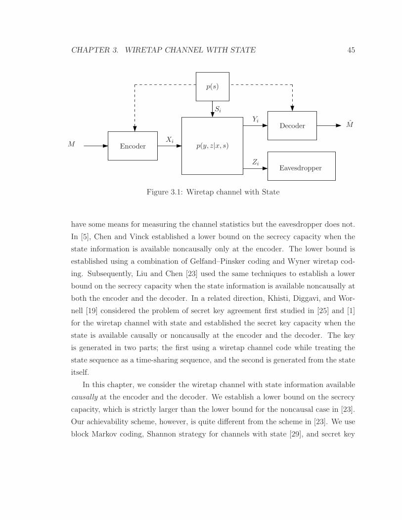
CHAPTER 3. WIRETAP CHANNEL WITH STATE 45
MXi
Si
Yi
Zi
M
Encoder
Decoder
Eavesdropper
p(s)
p(y, z|x, s)
Figure 3.1: Wiretap channel with State
have some means for measuring the channel statistics but the eavesdropper does not.
In [5], Chen and Vinck established a lower bound on the secrecy capacity when the
state information is available noncausally only at the encoder. The lower bound is
established using a combination of Gelfand–Pinsker coding and Wyner wiretap cod-
ing. Subsequently, Liu and Chen [23] used the same techniques to establish a lower
bound on the secrecy capacity when the state information is available noncausally at
both the encoder and the decoder. In a related direction, Khisti, Diggavi, and Wor-
nell [19] considered the problem of secret key agreement first studied in [25] and [1]
for the wiretap channel with state and established the secret key capacity when the
state is available causally or noncausally at the encoder and the decoder. The key
is generated in two parts; the first using a wiretap channel code while treating the
state sequence as a time-sharing sequence, and the second is generated from the state
itself.
In this chapter, we consider the wiretap channel with state information available
causally at the encoder and the decoder. We establish a lower bound on the secrecy
capacity, which is strictly larger than the lower bound for the noncausal case in [23].
Our achievability scheme, however, is quite different from the scheme in [23]. We use
block Markov coding, Shannon strategy for channels with state [29], and secret key
agreement from state information, which builds on the work in [19]. However, un-
like [19], we are not directly interested in the size of the secret key, but rather in using
the secret key generated from the state sequence in one transmission block to increase
the secrecy rate in the following block. This block Markov scheme causes additional
information leakage through the correlation between the secret key generated in a
block and the received sequences at the eavesdropper in subsequent blocks. We show
that this leakage is asymptotically negligible. Although a similar block Markov cod-
ing scheme was used in [2] to establish the secrecy capacity of the degraded wiretap
channel with rate limited secure feedback, in their setup no information about the
key is leaked to the eavesdropper because the feedback link is assumed to be secure.
We also establish an upper bound on the secrecy capacity of the wiretap channel with
state information available noncausally at the encoder and decoder. We show that
the upper bound coincides with the aforementioned lower bound for several classes
of channels. Thus, the secrecy capacity for these classes does not depend on whether
the state information is known causally or noncausally at the encoder.
The rest of the chapter is organized as follows. In Section 3.2, we provide the
needed definitions. In Section 3.3, we summarize and discuss the main results in
this chapter. The proofs of the lower and upper bounds are detailed in Sections 3.4
and 3.5, respectively.
3.2 Problem Definition
Consider a discrete memoryless wiretap channel (DM-WTC) with discrete memoryless
state (DM)
(X ×S, p(y, z|x, s)p(s),Y ,Z) that consists of a finite input alphabet X , finite output
alphabets Y , Z, a finite state alphabet S, a collection of conditional pmfs p(y, z|x, s)
on Y × Z, and a pmf p(s) on the state alphabet S. The sender X wishes to send a
confidential message M ∈ [1 : 2nR] to the receiver Y while keeping it secret from the
eavesdropper Z with either causal or noncausal state information available at both
the encoder and decoder.
A (2nR, n) code for the DM-WTC with causal state information at the encoder
46
CHAPTER 3. WIRETAP CHANNEL WITH STATE 47
and decoder consists of: (i) a message set [1 : 2nR], (ii) an encoder that generates a
symbol Xi(m) according to a conditional pmf p(xi|m, si, xi−1) for i ∈ [1 : n]; and a
decoder that assigns an estimate M or an error message to each received sequence pair
(yn, sn). We assume that the message M is uniformly distributed over the message
set. The probability of error is defined as P(n)e = P{M 6= M}. The information
leakage rate at the eavesdropper Z, which measures the amount of information about
M that leaks out to the eavesdropper, is defined as RL = 1nI(M ;Zn). A secrecy
rate R is said to be achievable if there exists a sequence of codes with P(n)e → 0
and RL → 0 as n → ∞. The secrecy capacity CS−CSI is the supremum of the set of
achievable rates.
We also consider the case when the state information is available noncausally at the
encoder. The only change in the above definitions is that the encoder now generates a
codeword Xn(m) according to a conditional pmf p(xn|m, sn), i.e., a random mapping
that depends on the entire state sequence instead of just the past and present state
sequence. The secrecy capacity for this scenario is denoted by CS−NCSI.
3.3 Summary of Main Results
We present the results in this chapter. The proofs of these results are given in the
following two sections and in the Appendix.
Lower Bound
The main result in this chapter is the following lower bound on the secrecy capacity
of the DM-WTC with state information available causally at both the encoder and
decoder.
Theorem 3.1. The secrecy capacity of the DM-WTC with state information available
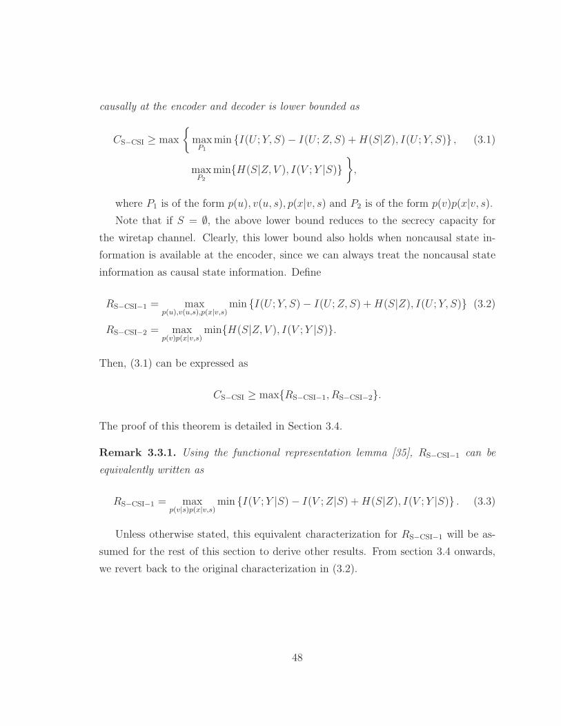
causally at the encoder and decoder is lower bounded as
CS−CSI ≥ max
{
maxP1
min {I(U ; Y, S)− I(U ;Z, S) +H(S|Z), I(U ; Y, S)} , (3.1)
maxP2
min{H(S|Z, V ), I(V ; Y |S)}
}
,
where P1 is of the form p(u), v(u, s), p(x|v, s) and P2 is of the form p(v)p(x|v, s).
Note that if S = ∅, the above lower bound reduces to the secrecy capacity for
the wiretap channel. Clearly, this lower bound also holds when noncausal state in-
formation is available at the encoder, since we can always treat the noncausal state
information as causal state information. Define
RS−CSI−1 = maxp(u),v(u,s),p(x|v,s)
min {I(U ; Y, S)− I(U ;Z, S) +H(S|Z), I(U ; Y, S)} (3.2)
RS−CSI−2 = maxp(v)p(x|v,s)
min{H(S|Z, V ), I(V ; Y |S)}.
Then, (3.1) can be expressed as
CS−CSI ≥ max{RS−CSI−1, RS−CSI−2}.
The proof of this theorem is detailed in Section 3.4.
Remark 3.3.1. Using the functional representation lemma [35], RS−CSI−1 can be
equivalently written as
RS−CSI−1 = maxp(v|s)p(x|v,s)
min {I(V ; Y |S)− I(V ;Z|S) +H(S|Z), I(V ; Y |S)} . (3.3)
Unless otherwise stated, this equivalent characterization for RS−CSI−1 will be as-
sumed for the rest of this section to derive other results. From section 3.4 onwards,
we revert back to the original characterization in (3.2).
48

CHAPTER 3. WIRETAP CHANNEL WITH STATE 49
In [23], the authors established the following lower bound for the noncausal case
CS−NCSI ≥ maxp(u|s)p(x|u,s)
(I(U ; Y, S)−max{I(U ;Z), I(U ;S)}) (3.4)
= maxp(u|s)p(x|u,s)
min {I(U ; Y |S)− I(U ;Z|S) + I(S;U |Z), I(U ; Y |S)} .
From (3.3), RS−CSI−1 is clearly at least as large as this lower bound. Hence, our lower
bound (3.1) is at least as large as this lower bound (3.4). We now show that the lower
bound (3.4) is as large as RS−CSI−1.
Fix V ∈ [0 : |V| − 1], p(v|s), and p(x|v, s) in RS−CSI−1. Let U ∈ [0 : |V||S| − 1] in
bound (3.4). Define the conditional probability mass functions: For u = v + s|V|, let
p(u|s) = p(v|s), p(x|u, s) = p(x|v, s), and let p(u|s) = p(x|u, s) = 0 otherwise. Under
this mapping, it is easy to see that H(S|Z, U) = 0 and the other terms in (3.4) reduce
to those in RS−CSI−1.
The following shows that our lower bound (3.1) can be strictly larger than (3.4).
Example: Consider the channel in Figure 3.2, where X ,Y ,Z,S ∈ {0, 1}, p(y, z|x, s) =
p(y, z|x), and the conditional pmf defined in the figure. The state S with entropy
H(S) = 1−H(0.1) is observed by both X and Y .
0.1
0.1
00
11
X Z Y
S
Figure 3.2: Example
By setting V = X independent of S and P{X = 1} = P{X = 0} = 0.5 in
RS−CSI−2, we obtain RS−CSI−2 ≥ 1−H(0.1).
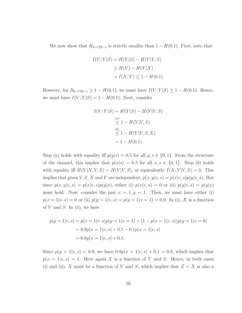
We now show that RS−CSI−1 is strictly smaller than 1−H(0.1). First, note that
I(V ; Y |S) = H(Y |S)−H(Y |V, S)
≤ H(Y )−H(Y |X)
= I(X ; Y ) ≤ 1−H(0.1).
However, for RS−CSI−1 ≥ 1 −H(0.1), we must have I(V ; Y |S) ≥ 1 −H(0.1). Hence,
we must have I(V ; Y |S) = 1−H(0.1). Next, consider
I(V ; Y |S) = H(Y |S)−H(Y |V, S)
(a)
≤ 1−H(Y |V, S)
(b)
≤ 1−H(Y |V, S,X)
= 1−H(0.1).
Step (a) holds with equality iff p(y|s) = 0.5 for all y, s ∈ {0, 1}. From the structure
of the channel, this implies that p(x|s) = 0.5 for all x, s ∈ {0, 1}. Step (b) holds
with equality iff H(Y |X, V, S) = H(Y |V, S), or equivalently I(X ; Y |V, S) = 0. This
implies that given V, S,X and Y are independent, p(x, y|v, s) = p(x|v, s)p(y|v, s). But
since p(x, y|v, s) = p(x|v, s)p(y|x), either (i) p(x|v, s) = 0 or (ii) p(y|v, s) = p(y|x)
must hold. Now, consider the pair x = 1, y = 1. Then, we must have either (i)
p(x = 1|v, s) = 0 or (ii) p(y = 1|v, s) = p(y = 1|x = 1) = 0.9. In (i), X is a function
of V and S. In (ii), we have
p(y = 1|v, s) = p(x = 1|v, s)p(y = 1|x = 1) + (1− p(x = 1|v, s))p(y = 1|x = 0)
= 0.9p(x = 1|v, s) + 0.1− 0.1p(x = 1|v, s)
= 0.8p(x = 1|v, s) + 0.1.
Since p(y = 1|v, s) = 0.9, we have 0.8p(x = 1|v, s) + 0.1 = 0.9, which implies that
p(x = 1|v, s) = 1. Here again X is a function of V and S. Hence, in both cases
(i) and (ii), X must be a function of V and S, which implies that Z = X is also a
50
CHAPTER 3. WIRETAP CHANNEL WITH STATE 51
function of V and S. Using the fact that p(x|s) = p(z|s) = 0.5 for all x, s, we have
I(V ;Z|S) = H(Z|S)−H(Z|V, S)
= H(X|S)
= 1.
The first expression in RS−CSI−1 is then upper bounded by
I(V ; Y |S)− I(V ;Z|S) +H(S|Z) ≤ I(V ; Y |S)− I(V ;Z|S) +H(S)
= 1−H(0.1)− 1 + 1−H(0.1)
= 1− 2H(0.1) < 1−H(0.1).
This shows that RS−CSI−1 < RS−CSI−2.
The proof of Theorem 3.1 is detailed in Section 3.4. To illustrate the main ideas,
we outline the proof for the characterization of RS−CSI−1 in (3.2) for the case when
I(U ; Y, S) − I(U ;Z, S) > 0. Our coding scheme involves the transmission of b − 1
independent messages over b n-transmission blocks. We split each message Mj , j ∈
[2 : b], into two independent messages Mj0 ∈ [1 : 2nR0] and Mj1 ∈ [1 : 2nR1] with
R0 +R1 = R. Codebook generation consists of two steps. The first is the generation
of the message codebook. We randomly generate sequences un(l), l ∈ [1 : 2nI(U ;Y,S)],
and partition the set of indices [1 : 2nI(U ;Y,S)] into 2nR0 equal size bins. The indices in
each bin are further partitioned into 2nR1 equal size sub-bins C(m0, m1). The second
step is to generate the key codebook. We randomly bin the set of state sequences
sn into 2nRK bins B(k). The key Kj−1 used in block j is the bin index of the state
sequence S(j − 1) in block j − 1.
To send message Mj , Mj1 is encrypted using the key Kj−1 to obtain M ′j1 = Mj1⊕
Kj−1. A codeword un(L) is selected uniformly at random from sub-bin C(Mj0,Mj1⊕
Kj−1) and transmitted using Shannon’s strategy as depicted in Figure 3.3. The
decoder uses joint typicality decoding together with its knowledge of the key to decode
message Mj at the end of block j. Finally, at the end of block j, the encoder and the
decoder declare the bin index Kj of the state sequence s(j) as the key to be used in
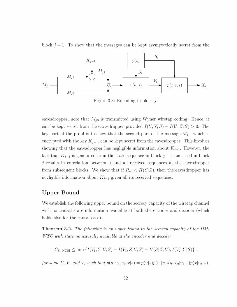
block j + 1. To show that the messages can be kept asymptotically secret from the
Mj
Mj1
Mj0
M ′j1
Kj−1
Ui
ViXi
p(s)
v(u, s) p(x|v, s)
Si
Si
Figure 3.3: Encoding in block j.
eavesdropper, note that Mj0 is transmitted using Wyner wiretap coding. Hence, it
can be kept secret from the eavesdropper provided I(U ; Y, S)− I(U ;Z, S) > 0. The
key part of the proof is to show that the second part of the message Mj1, which is
encrypted with the key Kj−1, can be kept secret from the eavesdropper. This involves
showing that the eavesdropper has negligible information about Kj−1. However, the
fact that Kj−1 is generated from the state sequence in block j − 1 and used in block
j results in correlation between it and all received sequences at the eavesdropper
from subsequent blocks. We show that if RK < H(S|Z), then the eavesdropper has
negligible information about Kj−1 given all its received sequences.
Upper Bound
We establish the following upper bound on the secrecy capacity of the wiretap channel
with noncausal state information available at both the encoder and decoder (which
holds also for the causal case).
Theorem 3.2. The following is an upper bound to the secrecy capacity of the DM-
WTC with state noncausally available at the encoder and decoder
CS−NCSI ≤ min {I(V1; Y |U, S)− I(V1;Z|U, S) +H(S|Z, U), I(V2; Y |S)} .
for some U, V1 and V2 such that p(u, v1, v2, x|s) = p(u|s)p(v1|u, s)p(v2|v1, s)p(x|v2, s).
52

CHAPTER 3. WIRETAP CHANNEL WITH STATE 53
The cardinality of the auxiliary random variables can be upper bounded by |U| ≤
|S|(|X |+ 1), |V1| ≤ |U||S|(|X |+ 1) and |V2| ≤ |V1||U||S||X |.
The proof of this theorem is given in Section 3.5.
Secrecy Capacity Results
We show that the upper bound in Theorem 3.2 coincides with the lower bound in
Theorem 3.1 for the following cases.
Class of less noisy channels
We show that Theorems 3.1 and 3.2 are also tight when I(U ; Y |S) ≥ I(U ;Z|S) for
every U such that (U, S) → (X,S) → (Y, Z) form a Markov chain, i.e., when Y is
less noisy than Z (see [20]) for every state s ∈ S [20].
Theorem 3.3. The secrecy capacity for the DM-WTC with the state information
available causally or noncausally at the encoder and decoder when Y is less noisy
than Z is
CS−CSI = CS−NCSI
= maxp(x|s)
min {I(X ; Y |S)− I(X ;Z|S) +H(S|Z), I(X ; Y |S)} .
Consider the special case when p(y, z|x, s) = p(y, z|x) and Z is a degraded version
of Y , then Theorem 3.3 specializes to the secrecy capacity for the wiretap channel
with a key [40]
CS−CSI = CS−NCSI
= maxp(x)
min {I(X ; Y )− I(X ;Z) +H(S), I(X ; Y )} .
Achievability for Theorem 3.3 follows directly from Theorem 3.1 by setting V =
X and observing RS−CSI−1 ≥ RS−CSI−2 since Y is less noisy than Z. Hence, the
achievability scheme for RS−CSI−1 is optimal for this class of channels. To establish
the converse, we use the less noisy assumption to strengthen the first inequality in
Theorem 3.2 as follows
I(V1; Y |U, S)− I(V1;Z|U, S) +H(S|Z, U) ≤ I(V1; Y |U, S)− I(V1;Z|U, S) +H(S|Z)
(a)
≤ I(V1; Y |S)− I(V1;Z|S) +H(S|Z)
(b)
≤ I(X ; Y |S)− I(X ;Z|S) +H(S|Z),
where (a), (b) follow from the less noisy assumption. The proof of the second inequal-
ity follows by the data processing inequality, which yields I(V2; Y |S) ≤ I(X ; Y |S).
Channel is independent of state and eavesdropper is less noisy than re-
ceiver
Next, consider the case where p(y, z|x, s) = p(y, z|x) and the eavesdropper Z is less
noisy than Y , that is, I(U ;Z) ≥ I(U ; Y ) for every U such that U → X → (Y, Z).
Then, the capacity of this special class of channels is
CS−CSI = CS−NCSI = maxp(x)
min{H(S), I(X ; Y )}.
Achievability follows by setting V = X independent of S. We note that the scheme
here is basically a “one-time pad” scheme where the message that is transmitted is
scrambled with a key generated from the state sequence. Here, the secrecy capacity
is achieved by RS−CSI−2, and hence, RS−CSI−2 ≥ RS−CSI−1. The example we gave to
illustrate the fact that RS−CSI−2 can be larger than RS−CSI−1 is a special case of this
class of channels. The converse follows from Theorem 3.2 and the observation that
since Z is less noisy than Y and p(y, z|x, s) = p(y, z|x),
I(V1; Y |U, S)− I(V1;Z|U, S) +H(S|Z, U) ≤ H(S|Z, U)
≤ H(S),
54
CHAPTER 3. WIRETAP CHANNEL WITH STATE 55
and I(V2; Y |S) ≤ I(X ; Y ).
Specific mutual information constraints
Following the lines of [5], we can show that Theorems 3.1 and 3.2 are tight for the
following two special cases. The achievability scheme for RS−CSI−1 is optimal for
both special cases.
(i) If there exists a V ∗ such that maxp(v|s)p(x|v,s)(I(V ; Y |S)−I(V ;Z|S)+H(S|Z)) =
I(V ∗; Y |S) − I(V ∗;Z|S) + H(S|Z) and I(V ∗; Y |S) − I(V ∗;Z|S) + H(S|Z) ≤
I(V ∗; Y |S), then the secrecy capacity is CS−CSI = CS−NCSI = I(V ∗; Y |S) −
I(V ∗;Z|S) +H(S|Z).
(ii) If there exists a V ′ such that maxp(v|s)p(x|v,s) I(V ; Y |S) = I(V ′; Y |S) and I(V ′; Y |S) ≤
I(V ′; Y |S)−I(V ′;Z|S)+H(S|Z), then the secrecy capacity is CS−CSI = CS−NCSI =
I(V ′; Y |S).
3.4 Proof of Theorem 3.1
We prove achievability of RS−CSI−1 and RS−CSI−2 separately. The proof of forRS−CSI−1
is split into Cases 1 and 2 while RS−CSI−2 is proved in Case 3.
Case 1: RS−CSI−1 with I(U ; Y, S) > I(U ;Z, S)
Codebook generation
Split messageMj into two independent messagesMj0 ∈ [1 : 2nR0 ] andMj1 ∈ [1 : 2nR1 ],
thus R = R0 +R1. Let R ≥ R. The codebook generation consists of two parts.
Message codeword generation: Randomly and independently generate sequences
un(l), l ∈ [1 : 2nR], each according to∏n
i=1 pU(ui) and partition the set of indices
[1 : 2nR] into 2nR0 equal-size bins C(m0), m0 ∈ [1 : 2nR0 ]. Further partition the
indices within each bin C(m0) into 2nR1 equal size sub-bins, C(m0, m1), m1 ∈ [1 :
2nR1]. Hence, l ∈ C(m0, m1) if and only if (m0 + m1 − 1 − 1)2n(R−R0−R1) + 1 ≤ l ≤
(m0 +m1)2n(R−R0−R1).
Key codebook generation: Randomly and uniformly partition the set of sn se-
quences into 2nRK bins B(k), k ∈ [1 : 2nRK ].
Both codebooks are revealed to all parties.
Encoding
We send b− 1 messages over b n-transmission blocks. In the first block, we randomly
select an index L ∈ C(m10, m′11). The encoder then computes vi = v(ui(L), si) and
transmits a randomly generated symbol Xi ∼ p(xi|si, vi) for i ∈ [1 : n]. At the end
of the first block, the encoder and the decoder declare k1 ∈ [1 : 2nRK ] such that
s(1) ∈ B(k1) as the key to be used in block 2.
Encoding in block j ∈ [2 : b] proceeds as follows. To send messagemj = (mj0, mj1)
and given key kj−1, the encoder computes m′j1 = mj1 ⊕ kj−1. To ensure secrecy, we
must have R1 ≤ RK [28]. The encoder then randomly selects an index L such that
L ∈ C(mj0, m′j1). It then computes vi = v(ui(L), si) and transmits a randomly
generated symbol Xi ∼ p(xi|si, vi) for i ∈ [(j − 1)n+ 1 : jn].
Decoding and analysis of the probability of error
At the end of block j, the decoder declares that l is sent if it is the unique index
such that (un(l),Y(j),S(j)) ∈ T(n)ǫ , otherwise it declares an error. It then finds the
index pair (mj0, m′j1) such that l ∈ C(mj0, m
′j1). Finally, it recovers mj1 by computing
mj1 = (m′j1 − kj−1)mod 2nRK .
To analyze the probability of error, let ǫ′′ > ǫ′ > ǫ > 0 and define the following
events for every j ∈ [2 : b]:
E(j) = {Mj 6= Mj},
E1(j) = {(Un(L),S(j)) /∈ T nǫ′ },
E2(j) = {(Un(L),S(j),Y(j)) /∈ T nǫ′′},
E3(j) = {(Un(l),S(j),Y(j)) ∈ T nǫ′′ for some l 6= L}.
56

CHAPTER 3. WIRETAP CHANNEL WITH STATE 57
The probability of error is upper bounded as
P(E) = P{∪bj=2E(j)} ≤
b∑
j=2
P(E(j)).
Each probability of error term can be upper bounded as
P(E(j)) ≤ P(E1(j)) + P(E2(j) ∩ E c1(j)) + P(E3(j) ∩ E c
2(j)).
Now, P(E1(j)) → 0 as n → ∞ by the law of large numbers (LLN) since P{(Un(L) ∈
T(n)ǫ )} → 1 as n → ∞ and S(j) ∼
∏ni=1 pS(si) =
∏ni=1 pS|U(si|ui) by independence.
The term P(E2(j) ∩ E c1(j)) → 0 as n → ∞ by LLN since (Un(L),S(j) ∈ T n
e′ and
Y n ∼∏n
i=1 pY |U, S(yi|ui, si). For the last term, consider
P(E3(j) ∩ E c2(j)) =
∑
l
p(l)P(E3(j) ∩ E c2(j)|L = l).
Note that L is independent of the transmission codebook sequences (un(l), l ∈ [1 :
2nR]) and the current state sequence S(j). Therefore, by the packing lemma [13,
Lecture 3], P(E3(j) ∩ E c2(j)|L = l) → 0 as n → ∞ if R < I(U ; Y, S)− δ(ǫ′′). Hence,
P(E3(j) ∩ E c2(j)) → 0 as n → ∞ if R < I(U ; Y, S)− δ(ǫ′′).
Analysis of the information leakage rate
Let Z(j) denote the eavesdropper’s received sequence in block j ∈ [1 : b] and Zj =
(Z(1), . . . ,Z(j)). We will need the following two results.
Proposition 3.1. If RK < H(S|Z) − 4δ(ǫ) and R ≥ I(U ;Z, S) + δ(ǫ), then the
following holds for every j ∈ [1 : b].
1. H(Kj|C) ≥ n(RK − δ(ǫ)).
2. I(Kj;Z(j)|C) ≤ n(δ′(ǫ) + δ′′(ǫ)). .
3. I(Kj;Zj |C) ≤ nδ′′′(ǫ), where δ′(ǫ) → 0, δ′′(ǫ) → 0 and δ′′′(ǫ) → 0 as ǫ → 0.
The proof of this proposition is given in Appendix B.1.
The second result is Lemma 2.1 from Chapter 2, which we restate here for conve-
nience.
Lemma 3.1. Let (U, V, Z) ∼ p(u, v, z), R ≥ 0, and ǫ > 0. Let Un be a random
sequence distributed according to∏n
i=1 pU(ui). Let V n(l), l ∈ [1 : 2nR], be a set of
random sequences that are conditionally independent given Un and each distributed
according to∏n
i=1 pV |U(vi|ui). Define C = {Un, V n(l)}. Let L ∈ [1 : 2nR] be a
random index distributed according to an arbitrary pmf. Then, if P{(Un, V n(L), Zn) ∈
T(n)ǫ } → 1 as n → ∞ and R > I(V ;Z|U) + δ(ǫ), there exists a δ′(ǫ) > 0, where
δ′(ǫ) → 0 as ǫ → 0, such that, for n sufficiently large, H(L|Zn, Un, C) ≤ n(R −
I(V ;Z|U)) + nδ′(ǫ).
We are now ready to upper bound the leakage rate averaged over codes. Consider
I(M2,M3, . . . ,Mb;Zb|C) =
b∑
j=2
I(Mj ;Zb|C,M b
j+1)
(a)
≤b∑
j=2
I(Mj ;Zb|C,S(j),M b
j+1)
(b)=
b∑
j=2
I(Mj ;Zj|C,S(j)),
where (a) follows by the independence of Mj and (S(j),M bj+1), and (b) follows by
the Markov Chain relationship (Zbj+1,M
bj+1, C) → (Zj ,S(j), C) → (Mj, C). Hence, it
suffices to upper bound each individual term I(Mj ;Zj|C,S(j)). Consider
I(Mj ;Zj|C,S(j)) = I(Mj0,Mj1;Z
j |C,S(j))
= I(Mj0,Mj1;Zj−1|C,S(j)) + I(Mj0,Mj1;Z(j)|C,S(j),Z
j−1).
58
CHAPTER 3. WIRETAP CHANNEL WITH STATE 59
Note that the first term is equal to zero by the independence of Mj and past trans-
missions, the codebook, and state sequence. For the second term, we have
I(Mj0,Mj1;Z(j)|C,S(j),Zj−1) = I(Mj0;Z(j)|C,S(j),Z
j−1)
+ I(Mj1;Z(j)|C,Mj0,S(j),Zj−1).
We now bound each term separately. Consider the first term
I(Mj0;Z(j)|C,S(j),Zj−1) = I(Mj0, L;Z(j)|C,S(j),Z
j−1)
− I(L;Z(j)|C,Mj0,S(j),Zj−1)
≤ I(Un;Z(j)|C,S(j),Zj−1)−H(L|C,Mj0,S(j),Zj−1)
+H(L|C,Z(j),Mj0,S(j))
≤n∑
i=1
(H(Zi(j)|C,Si(j))−H(Zi(j)|C, Ui,Si(j)))
−H(L|C,Mj0,S(j),Zj−1) +H(L|C,Z(j),Mj0,S(j))
(a)
≤ nI(U ;Z|S)−H(L|C,Mj0,S(j),Zj−1)
+H(L|C,Z(j),Mj0,S(j))
(b)
≤ nI(U ;Z|S)−H(L|C,Mj0,S(j),Zj−1)
+ n(R −R0 − I(U ;Z, S) + δ′(ǫ))
(c)= n(R− R0)−H(L|C,Mj0,S(j),Z
j−1) + nδ′(ǫ)
= n(R −R0)−H(Mj1 ⊕Kj−1|C,Mj0,S(j),Zj−1)
−H(L|C,Mj0,S(j),Zj−1,Mj1 ⊕Kj−1) + nδ′(ǫ)
≤ n(R− R0)−H(Mj1 ⊕Kj−1|C,Mj0,S(j), Kj−1,Zj−1)
− n(R− R0 −RK) + nδ′(ǫ)
(d)= nRK −H(Mj1 ⊕Kj−1|C,Mj0,S(j), Kj−1) + nδ′(ǫ)
= nRK −H(Mj1|C,Mj0,S(j), Kj−1) + nδ′(ǫ)
= nδ′(ǫ),
where (a) follows from the fact that H(Zi(j)|C,Si(j)) ≤ H(Zi(j)|Si(j)) = H(Z|S)
and H(Zi(j)|C, Ui,Si(j)) = H(Z|U, S). Step (b) follows by Lemma 3.1 which requires
that (i) P{(Un(L),S(j),Z(j)) ∈ T(n)ǫ } → 1 as n → ∞, and (ii) R−R0 > I(U ;Z, S)+
δ(ǫ); (i) can be established using the same steps as in the analysis of probability of
error. Step (c) follows by the independence of U and S. Step (d) follows by the Markov
Chain relationship (Zj−1,Mj0,S(j)) → (Kj−1,Mj0,S(j)) → (Mj1 ⊕Kj−1,Mj0,S(j)).
The last step follows by the fact that Mj1 is independent of (C,Mj0,S(j), Kj−1) and
uniformly distributed over [1 : 2nRK ].
Next, consider the second term
I(Mj1;Z(j)|C,Mj0,S(j),Zj−1) ≤ I(Mj1, L;Z(j)|C,Mj0,S(j),Z
j−1)
− I(L;Z(j)|C,Mj0,Mj1,S(j),Zj−1)
≤ I(Un;Z(j)|C,Mj0,S(j),Zj−1)
−H(L|C,Mj0,Mj1,S(j),Zj−1)
+H(L|C,Mj0,Mj1,S(j),Zj)
(a)
≤ nI(U ;Z|S)−H(L|C,Mj0,Mj1,S(j),Zj−1)
+H(L|C,Mj0,Mj1,S(j),Zj)
(b)
≤ nI(U ;Z|S)−H(L|C,Mj0,Mj1,S(j),Zj−1)
+ n(R− R0)− nI(U ;Z, S) + nδ′(ǫ)
= n(R− R0)−H(L|C,Mj0,Mj1,S(j),Zj−1)
+ nδ′(ǫ),
where (a) follows from the same steps used in bounding I(Mj0;Z(j)|C,S(j),Zj−1) and
(b) follows from Lemma 3.1, which requires the same condition R−R0 > I(U ;Z, S)+
δ(ǫ). Next consider
H(L|C,Mj0,Mj1,S(j),Zj−1) = H(Mj1 ⊕Kj−1|C,Mj0,Mj1,S(j),Z
j−1)
+H(L|C,Mj0,Mj1,Mj1 ⊕Kj−1,S(j),Zj−1)
= H(Kj−1|C,Mj0,Mj1,S(j),Zj−1)
60
CHAPTER 3. WIRETAP CHANNEL WITH STATE 61
+ n(R− R0 − RK)
= H(Kj−1|C,Zj−1) + n(R− R0 −RK).
From Proposition 3.1, H(Kj−1|C,Zj−1) ≥ n(RK − δ(ǫ)− δ′′′(ǫ)), which implies that
I(Mj1;Z(j)|C,Mj0,S(j),Zj−1) ≤ n(δ(ǫ) + δ′(ǫ)) + nδ′′′(ǫ).
This completes the analysis of the information leakage rate.
Rate analysis
From the analysis of probability of error and information leakage rate, we see that
the rate constraints are
R < I(U ; Y, S)− δ(ǫ),
R−R0 > I(U ;Z, S) + δ(ǫ),
RK < H(S|Z)− 4δ(ǫ),
R0 +R1 ≤ R,
R1 ≤ RK ,
R = R0 +R1,
R ≥ 0, R0 ≥ 0, R1 ≥ 0, RK ≥ 0.
Using Fourier-Motzkin elimination (e.g., see Lecture 6 of [13]), we obtain
R < maxp(u),v(u,s),p(x|s,v)
min {I(U ; Y, S)− I(U ;Z, S) +H(S|Z), I(U ; Y, S)}
(a)= max
p(u),v(u,s),p(x|s,v)min {I(V ; Y |S)− I(V ;Z|S) +H(S|Z), I(V ; Y |S)} ,
where (a) follows by the independence of U and S and the fact that V is a function
of U and S.
Case 2: RS−CSI−1 with I(U ; Y, S) ≤ I(U ;Z, S)
In this case, only part of the key generated from the previous block is used to encrypt
the message transmitted to the eavesdropper. The other part of the key is used to
generate additional uncertainty about the message sent at the eavesdropper to ensure
that a sufficiently large secret key rate is achieved in the current block. Note that we
only need to consider the case where H(S|Z)− (I(U ;Z, S)− I(U ; Y, S)) > 0.
Codebook generation
Codebook generation again consists of two parts.
Message codebook generation: Let R ≥ Rd and R ≤ R − Rd. Randomly and
independently generate sequences un(l), l ∈ [1 : 2nR], each according to∏n
i=1 pU(ui)
and partition the set of indices [1 : 2nR] into 2nRd equal-size bins C(md), md ∈
[1 : 2nRd]. We further partition the set of indices in each bin C(md) into sub-bins,
C(md, m), m ∈ [1 : 2nR].
Key codebook generation: We randomly bin the set of sn ∈ Sn sequences into 2nRK
bins B(k), k ∈ [1 : 2nRK ].
Encoding
We send b− 1 messages over b n-transmission blocks. In the first block, we randomly
select an index L. The encoder then computes vi = v(ui(L), si), i ∈ [1 : n], and
transmits a randomly generates sequence Xn according to∏n
i=1 pX|S,V (xi|si, vi). At
the end of the first block, the encoder and decoder declare k1 ∈ [1 : 2nRK ] such that
s(1) ∈ B(k1) as the key to be used in block 2.
Encoding in block j ∈ [2 : b] is as follows. We split the key kj−1 into two indepen-
dent parts, Kj−1,d and Kj−1,m at rates Rd and R, respectively. To send message mj ,
the encoder computes m′ = mj ⊕ k(j−1)m. This requires that RK ≥ R +Rd. The en-
coder then randomly selects an index L ∈ C(k(j−1)d, m′). At time i ∈ [(j−1)n+1 : jn],
it computes vi = (ui(L), si), i ∈ [1 : n], and transmits a randomly generated sequence
Xn according to∏n
i=1 pX|S,V (xi|si, vi).
62
CHAPTER 3. WIRETAP CHANNEL WITH STATE 63
Decoding and analysis of the probability of error
At the end of block j, the decoder declares that l is sent if it is the unique index such
that (un(l),Y(j),S(j)) ∈ T(n)ǫ and l ∈ C(k(j−1)d). Otherwise, it declares an error. It
then finds the index m′ such that un(l) ∈ C(k(j−1)d, m′). Finally, it recovers mj by
computing mj = (m′ − k(j−1)m)mod 2nR . Following similar steps to the analysis for
Case 1, it can be shown that Pe → 0 as n → ∞ if R− Rd < I(U ; Y, S)− δ(ǫ).
Analysis of the information leakage rate
Following the same steps as for Case 1, we can show that it suffices to upper bound
the terms I(Mj ;Z(j)|C,S(j),Zj−1) for j ∈ [2 : b]. Define M ′
j = Mj ⊕ K(j−1)m and
consider
I(Mj ;Z(j)|C,S(j),Zj−1) = H(Mj)−H(Mj |C,S(j),Z
j)
≤ H(Mj)−H(Mj|C,S(j), K(j−1)d,M′j,Z
j)
= H(Mj)−H(Mj |C, K(j−1)d,M′j ,Z
j−1)
= H(Mj)−H(Mj |C,Zj−1, K(j−1)d)
−H(M ′j |C,Z
j−1, K(j−1)d,Mj) +H(M ′j|C,Z
j−1, K(j−1)d)
= nR −H(Mj) +H(M ′j|C,Z
j−1, K(j−1)d)
−H(M ′j|C,Z
j−1, K(j−1)d,Mj)
≤ nR−H(K(j−1)m|C,Zj−1, K(j−1)d).
Next, we show that
I(K(j−1)m;Zj−1|C, K(j−1)d) ≤ nδ′′′(ǫ), (3.5)
H(K(j−1)m|C, K(j−1)d) ≥ n(RK −Rd − δ(ǫ)), (3.6)
which implies
I(Mj ;Z(j)|C,S(j),Zj−1) ≤ nR − n(RK − Rd) + n(δ′′′(ǫ) + δ(ǫ)).

Hence, the rate of information leakage tends to zero as n → ∞ if R ≤ RK − Rd. To
prove (3.5) and (3.6), we need the following.
Proposition 3.2. If R > I(U ;Z, S) + δ(ǫ) and RK < H(S|Z) − 4δ(ǫ), then for all
j ∈ [1 : b],
1. H(Kj|C) ≥ n(RK − δ(ǫ)).
2. I(Kj;Z(j)|C) ≤ n(δ(ǫ) + δ′(ǫ) + δ′′(ǫ)).
3. I(Kj;Zj |C) ≤ nδ′′′(ǫ), where δ′(ǫ) → 0, δ′′(ǫ) → 0 and δ′′′(ǫ) → 0 as ǫ → 0.
The proof of this proposition is given in Appendix B.2.
Part 3 of Proposition 3.2 implies (3.5) since
I(Kj−1;Zj−1|C) = I(K(j−1)d, K(j−1)m;Z
j−1|C)
= I(K(j−1)d;Zj−1|C) + I(K(j−1)m;Z
j−1|C, K(j−1)d).
Part 1 of Proposition 3.2 implies (3.6) sinceH(K(j−1)|C) = H(K(j−1)m, K(j−1)d|C) ≥
n(RK − δ(ǫ)), which implies that H(K(j−1)m|C, K(j−1)d) ≥ n(RK − Rd − δ(ǫ)).
Rate analysis
The following rate constraints are necessary for Case 2.
R > I(U ;Z, S) + δ(ǫ),
R −Rd < I(U ; Y, S)− δ(ǫ),
R ≤ R− Rd,
RK < H(S|Z)− 4δ(ǫ),
R ≤ RK −Rd,
R ≥ 0, RK ≥ 0, Rd ≥ 0, R ≥ 0.
Using Fourier Motzkin elimination, we obtain
R < maxp(u),v(u,s),p(x|s,v)
min {I(U ; Y, S)− I(U ;Z, S) +H(S|Z), I(U ; Y, S)}
64
CHAPTER 3. WIRETAP CHANNEL WITH STATE 65
= maxp(u),v(u,s),p(x|s,v)
min {I(V ; Y |S)− I(V ;Z|S) +H(S|Z), I(V ; Y |S)} .
Case 3: RS−CSI−2
Achievability of RS−CSI−2 uses the same techniques as Case 2 for RS−CSI−1. However,
here the key generated in a block is used only to encrypt the message in the follow-
ing block. The eavesdropper may be able to decode the message transmitted in a
block, which would reduce the key rate generated at the end of that block. This is
compensated for by the fact that the entire key is used for encryption. The code-
book generation, encoding and analysis of probability of error and equivocation are
therefore similar to that in Case 2.
As an outline, in each block, we generate a key Kj of size 2nH(S|V,Z). In the next
block, we encrypt the message Mj+1 using Kj to obtain M ′j+1 = Mj+1 ⊕ Kj. A
codeword V n(M ′j+1) is then selected from a codebook of size less than 2nI(V ;Y,S). This
codeword is then transmitted by generating Xi according to pX(Vi, Si) for i ∈ [1 : n].
The decoder first decodes M ′j+1 using (Y(j + 1),S(j + 1)) and then decrypts the
message using Mj+1 = (M ′j+1 −Kj)mod 2nRK .
Remark 3.4.1. An important difference between the schemes for achieving RS−CSI−1
and RS−CSI−2 is that the transmitted codeword in the scheme for RS−CSI−1 can be
kept secret from the eavesdropper through a combination of Wyner wiretap coding and
encryption of the codebook using the secret key. This fact was made clear in Case 2 of
the proof, where part of the key was explicitly used to encrypt the codebook instead of
the message. On the other hand, no effort was made to keep the transmitted codeword
secret from the eavesdropper in the scheme for RS−CSI−2. Hence, one cannot assume
that the eavesdropper has no information about the codeword sent. As such, we did
not use the Shannon strategy as in Figure 3.1 in the encoding part for RS−CSI−2. If
we had used the Shannon strategy, we would have obtained the expression
R′S−CSI−2 = max
p(u),v(u,s),p(x|s,v){H(S|Z, U), I(U ; Y, S)}
= maxp(u),v(u,s),p(x|s,v)
{H(S|Z, U), I(V ; Y |S)}.
The first term in R′S−CSI−2, H(S|Z, U), is the rate of the secret key rate generated
assuming that the eavesdropper knows the transmitted codeword. As a result of this
term, R′S−CSI−2 is simply a special case of our original RS−CSI−2 expression, where
we maximized the rate over p(v) (V independent of S). This is in contrast to the
equivalent characterization of RS−CSI−1 in (3.3), where we were able to perform the
maximization of the rate over p(v|s).
We now turn to the proof of achievability of RS−CSI−2.
Codebook generation
Codebook generation again consists of two parts.
Message codebook generation: Randomly and independently generate sequences
vn(l), l ∈ [1 : 2nR], each according to∏n
i=1 pV (vi).
Key codebook generation: Set RK = R. Randomly bin the set of sn ∈ Sn sequences
into 2nRK bins B(k), k ∈ [1 : 2nRK ].
Encoding
We send b− 1 messages over b n-transmission blocks. In the first block, we randomly
select an index L ∈ [1 : 2nR]. The encoder then selects vn(L) transmits a randomly
generated sequence Xn according to∏n
i=1 pX|S,V (xi|si, vi). At the end of the first
block, the encoder and the decoder declare the index k1 ∈ [1 : 2nRK ] such that
s(1) ∈ B(k1) as the key to be used in block 2.
Encoding in block j ∈ [2 : b] is as follows. To send message mj , the encoder
computes the encrypted message m′ = mj⊕kj−1. It then selects the sequence vn(m′).
At time i ∈ [(j − 1)n + 1 : jn], it transmits a randomly generated sequence Xn
according to∏n
i=1 pX|S,V (xi|si, vi).
Decoding and analysis of the probability of error
At the end of block j, the decoder declares that m′ is sent if it is the unique index such
that (vn(m′),Y(j),S(j)) ∈ T(n)ǫ . Otherwise, it declares an error. It then recovers mj
66
CHAPTER 3. WIRETAP CHANNEL WITH STATE 67
by computing mj = (m′ − kj−1)mod 2nRK . Following similar steps to the analysis for
Case 1, it can be shown that the probability of error tends to zero as n → ∞ if
R < I(V ; Y, S)− δ(ǫ).
Analysis of the information leakage rate
Following the same steps as for Case 1, we can show that it suffices to upper bound
the terms I(Mj ;Z(j)|C,S(j),Zj−1) for j ∈ [2 : b]. Consider
I(Mj;Z(j)|C,S(j),Zj−1) = H(Mj)−H(Mj |C,S(j),Z
j)
≤ H(Mj)−H(Mj|C,S(j),Mj ⊕Kj−1,Zj)
= H(Mj)−H(Mj |C,Mj ⊕Kj−1,Zj−1)
= H(Mj)−H(Mj ⊕Kj−1,Mj |C,Zj−1)
+H(Mj ⊕Kj−1|C,Zj−1)
≤ nR−H(Mj|C,Zj−1)
−H(Mj ⊕Kj−1|C,Zj−1,Mj) + nR
= nR −H(Kj−1|C,Zj−1).
Next, we show that
I(Kj−1;Zj−1|C) ≤ nδ′′(ǫ), (3.7)
H(Kj−1|C) ≥ n(RK − δ(ǫ)). (3.8)
which would imply
I(Mj ;Z(j)|C,S(j),Zj−1) ≤ n(δ′′(ǫ) + δ(ǫ)).
To prove (3.7) and (3.8), we will use the following.
Proposition 3.3. If RK < H(S|Z, V )− 4δ(ǫ), then for all j ∈ [1 : b],
1. H(Kj|C) ≥ n(RK − δ(ǫ)).
2. I(Kj;Z(j)|C) ≤ nδ′(ǫ).
3. I(Kj;Zj |C) ≤ nδ′′(ǫ), where δ′(ǫ) → 0 and δ′′(ǫ) → 0 as ǫ → 0.
The proof of this proposition is given in Appendix B.3. It is clear that equa-
tions (3.7) and (3.8) are implied by Proposition 3.3, which completes the analysis of
information leakage rate.
Rate analysis
The following rate constraints are necessary for Case 3.
R = RK ,
R < I(V ; Y, S)− δ(ǫ),
RK < H(S|Z, V )− 4δ(ǫ),
RK ≥ 0, R ≥ 0.
Using Fourier Motzkin elimination, these constraints imply the achievability of
R < maxp(v)p(x|s,v)
min{H(S|Z, V ), I(V ; Y |S)}.
3.5 Proof of Theorem 3.2
For any sequence of codes with probability of error and leakage rate that approach
zero as n → ∞, consider
nR = H(M)
(a)
≤ I(M ; Y n, Sn) + nǫn
(b)
≤ I(M ; Y n, Sn)− I(M ;Zn) + 2nǫn
=
n∑
i=1
(
I(M ; Yi, Si|Yni+1, S
ni+1)− I(M ;Zi|Z
i−1))
+ 2nǫn
68
CHAPTER 3. WIRETAP CHANNEL WITH STATE 69
(c)=
n∑
i=1
(
I(M,Z i−1; Yi, Si|Yni+1, S
ni+1)− I(M,Y n
i+1, Sni+1;Zi|Z
i−1))
+ 2nǫn
(d)=
n∑
i=1
(
I(M ; Yi, Si|Yni+1, S
ni+1, Z
i−1)− I(M ;Zi|Yni+1, S
ni+1, Z
i−1))
+ 2nǫn
(e)=
n∑
i=1
(I(V1i; Yi, Si|Ui)− I(V1i;Zi|Ui)) + 2nǫn
=
n∑
i=1
(I(V1i; Yi, Si|Ui)− I(V1i;Zi, Si|Ui) + I(V1i;Si|Zi, Ui)) + 2nǫn
≤n∑
i=1
(I(V1i; Yi, Si|Ui)− I(V1i;Zi, Si|Ui) +H(Si|Zi, Ui)) + 2nǫn
≤n∑
i=1
(I(V1i; Yi|Ui, Si)− I(V1i;Zi, Si|Ui, Si) +H(Si|Zi, Ui)) + 2nǫn
(f)= n(I(V1; Y |U, S)− I(V1;Z|U, S)) + nH(S|Z, U) + 2nǫn,
where (a) follows by Fano’s inequality; (b) follows by the secrecy condition; (c)
and (d) follow by the Csiszar sum identity; (e) follows by the identifications Ui =
(Y ni+1, S
ni+1, Z
i−1) and V1i = (M,Y ni+1, S
ni+1, Z
i−1); and (f) follows by using the time-
sharing random variable Q and defining U = (UQ, Q), V1 = (V1Q, Q), S = SQ, Y = YQ
and Z = ZQ.
For the second upper bound, we have
nR ≤ I(M ; Y n, Sn) + nǫn
(a)= I(M ; Y n|Sn) + nǫn
=n∑
i=1
I(M ; Yi|Sn, Y n
i+1)
≤n∑
i=1
I(M,Y ni+1, Z
i−1, Sni+1, S
i−1; Yi|Si)
(b)=
n∑
i=1
I(V2i; Yi|Si)
= nI(V2Q; Y |S,Q)

(c)
≤ nI(V2; Y |S),
where (a) follows by the independence of M and Sn; (b) follows by the identification
V2i = (M,Y ni+1, Z
i−1, Sni+1, S
i−1); and (c) follows by defining V2 = (V2Q, Q). The
bounds on cardinality of the auxiliary random variables follow from standard tech-
niques (e.g., see [13, Appendix C]).
3.6 Summary of Chapter
We established bounds on the secrecy capacity of the wiretap channel with state
information causally available at the encoder and the decoder. We showed that our
lower bound can be strictly larger than the best known lower bound for the noncausal
state information case. The upper bound holds when the state information is available
noncausally at the encoder and the decoder. We showed that the bounds are tight
for several classes of wiretap channels with state.
As we have seen, the secrecy capacity for several special classes of the wiretap
channels with state available at both the encoder and the decoder does not depend
on whether the state is available causally or noncausally. An interesting question to
explore is whether this observation holds in general for our setup.
We used key generation from state information to improve the message transmis-
sion rate. It may be possible to extend this idea to the case when the state information
is available only at the encoder. This case, however, is not straightforward to analyze
since it would be necessary for the encoder to reveal some state information to the
decoder (and hence partially to the eavesdropper) in order to agree on a secret key,
which would reduce the wiretap coding part of the rate.
70
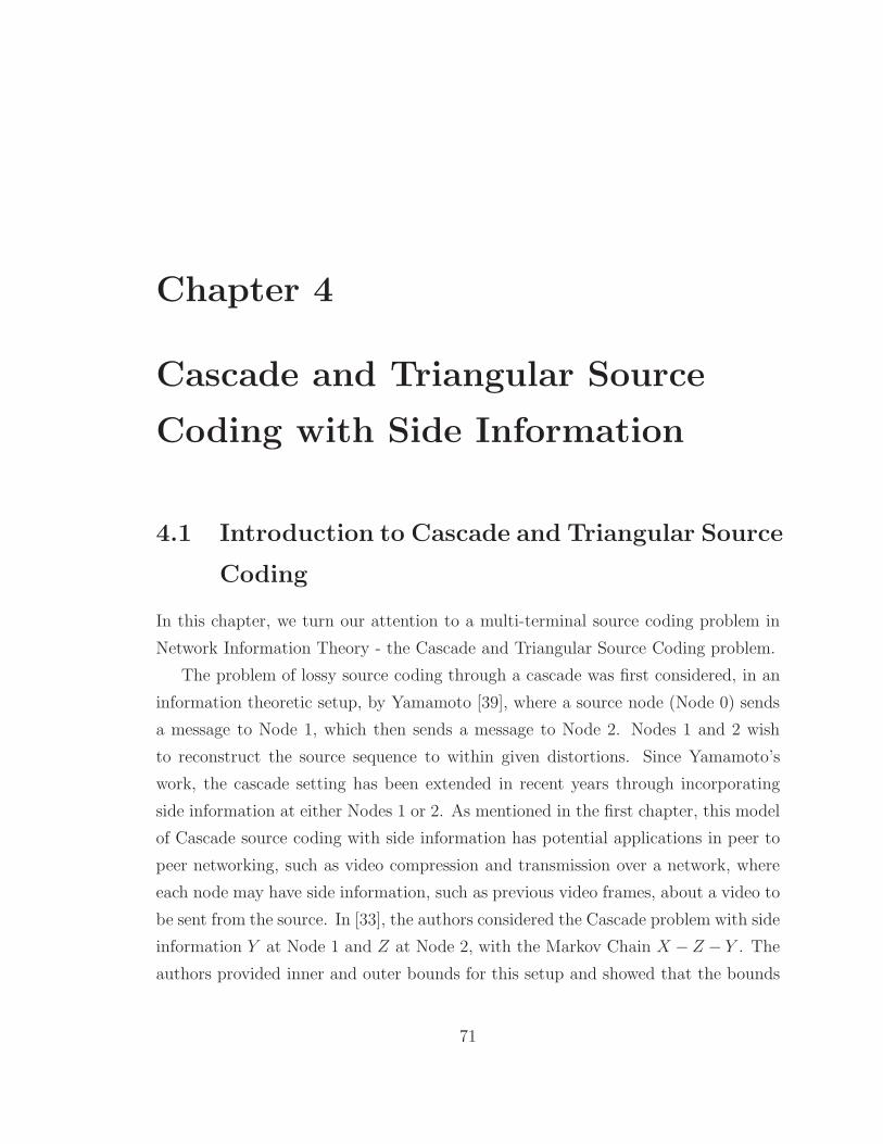
Chapter 4
Cascade and Triangular Source
Coding with Side Information
4.1 Introduction to Cascade and Triangular Source
Coding
In this chapter, we turn our attention to a multi-terminal source coding problem in
Network Information Theory - the Cascade and Triangular Source Coding problem.
The problem of lossy source coding through a cascade was first considered, in an
information theoretic setup, by Yamamoto [39], where a source node (Node 0) sends
a message to Node 1, which then sends a message to Node 2. Nodes 1 and 2 wish
to reconstruct the source sequence to within given distortions. Since Yamamoto’s
work, the cascade setting has been extended in recent years through incorporating
side information at either Nodes 1 or 2. As mentioned in the first chapter, this model
of Cascade source coding with side information has potential applications in peer to
peer networking, such as video compression and transmission over a network, where
each node may have side information, such as previous video frames, about a video to
be sent from the source. In [33], the authors considered the Cascade problem with side
information Y at Node 1 and Z at Node 2, with the Markov Chain X −Z − Y . The
authors provided inner and outer bounds for this setup and showed that the bounds
71
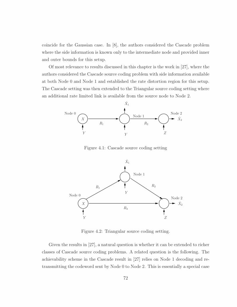
coincide for the Gaussian case. In [8], the authors considered the Cascade problem
where the side information is known only to the intermediate node and provided inner
and outer bounds for this setup.
Of most relevance to results discussed in this chapter is the work in [27], where the
authors considered the Cascade source coding problem with side information available
at both Node 0 and Node 1 and established the rate distortion region for this setup.
The Cascade setting was then extended to the Triangular source coding setting where
an additional rate limited link is available from the source node to Node 2.
X
Y Y Z
R1 R2
X1
X2
Node 0Node 1
Node 2
Figure 4.1: Cascade source coding setting
X
Y
Y
Z
R1R2
R3
X1
X2
Node 0
Node 1
Node 2
Figure 4.2: Triangular source coding setting.
Given the results in [27], a natural question is whether it can be extended to richer
classes of Cascade source coding problems. A related question is the following. The
achievability scheme in the Cascade result in [27] relies on Node 1 decoding and re-
transmitting the codeword sent by Node 0 to Node 2. This is essentially a special case
72

CHAPTER 4. CASCADE AND TRIANGULAR SOURCE CODING 73
of the decode and re-bin scheme where Node 1 decodes and re-bins the codeword sent
by Node 0 to Node 2. When is this decode and re-bin scheme optimum and what is
the statistical structure of the sources and network topology required for this scheme
to be optimum? In this chapter, we extend the Cascade and Triangular source coding
setting in [27] to include additional side information Z at Node 2, with the constraint
that the Markov chain X − Y −Z holds. Under the Markov constraint, we establish
the rate distortion regions for both the Cascade and Triangular setting. The Cascade
and Triangular settings are shown in Figures 4.1 and 4.2, respectively. In the Cascade
case, we show that, at Node 1, the decode and re-bin scheme is optimum. To the best
of our knowledge, this is the first lossy source coding setting where the decode and
re-bin scheme at the Cascade is shown to be optimum. (In [16], the decode and re-bin
scheme was shown to be optimum for some classes of source statistics in a lossless
setting.) The decode and re-bin appears to rely quite heavily on the fact that the side
information at Node 2 is degraded: Since Node 1 can decode any codeword intended
for Node 2, there is no need for Node 0 to send additional information for Node 1
to relay to Node 2 on the R1 link. Node 0 can therefore tailor the transmission for
Node 1 and rely on Node 1 to decode and minimize the rate required on the R2 link.
We also extend our results to two way source coding through a cascade, where Node
0 wishes to obtain a lossy version of Z through a rate limited link from Node 2 to
Node 0. This setup generalizes the (two rounds) two way source coding result found
in [17]1. The Two Way Cascade Source Coding and Two Way Triangular Source
Coding are given in Figures 4.3 and 4.4, respectively.
The rest of this chapter is as follows. In section 4.2, we provide the formal defi-
nitions and problem setup. In section 4.3, we present and prove our results for the
aforementioned settings. In section 4.4, we consider the Quadratic Gaussian case. We
show that Gaussian auxiliary random variables suffice to exhaust the rate distortion
regions and their parameters may be found through solving a tractable low dimen-
sional optimization problem. We also showed that our Quadratic Gaussian settings
may be transformed into equivalent settings in [27] where explicit characterizations
1 [17] considered multiple rounds. In this chapter, we consider only two rounds and when wemention the results in [17], we mean the two rounds version of the results
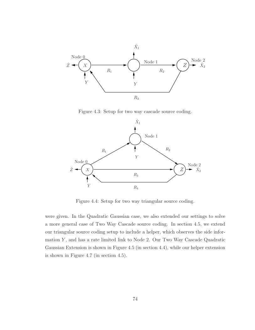
X
Y Y
R1 R2
R3
X1
X2ZZ
Node 0Node 1 Node 2
Figure 4.3: Setup for two way cascade source coding.
X
Y
Y
R1R2
R3
R4
X1
X2ZZ
Node 0
Node 1
Node 2
Figure 4.4: Setup for two way triangular source coding.
were given. In the Quadratic Gaussian case, we also extended our settings to solve
a more general case of Two Way Cascade source coding. In section 4.5, we extend
our triangular source coding setup to include a helper, which observes the side infor-
mation Y , and has a rate limited link to Node 2. Our Two Way Cascade Quadratic
Gaussian Extension is shown in Figure 4.5 (in section 4.4), while our helper extension
is shown in Figure 4.7 (in section 4.5).
74
CHAPTER 4. CASCADE AND TRIANGULAR SOURCE CODING 75
4.2 Problem Definition
In this section, we give formal definitions for the setups under consideration. The
source sequences under consideration, {Xi ∈ X , i = 1, 2, . . .}, {Yi ∈ Y , i = 1, 2, . . .}
and {Zi ∈ Z, i = 1, 2, . . .}, are drawn from finite alphabets X , Y and Z respectively.
For any i ≥ 1, the random variables (Xi, Yi, Zi) are independent and identically
distributed according to p(x, y, z) = p(x)p(y|x)p(z|y); i.e. X−Y −Z. The distortion
measure between sequences is defined in the usual way. Let d : X × X → [0,∞).
Then,
d(xn, xn) :=1
n
n∑
i=1
d(xi, xi).
4.2.1 Cascade and Triangular Source coding
We give formal definition for the Triangular source coding setting (Figure 4.2). The
Cascade setting follows from specializing the definitions for the Triangular setting by
setting R3 = 0. A (n, 2nR1 , 2nR2, 2nR3) code for the Triangular setting consists of 3
encoders
f1 (at Node 0) : X n ×Yn → M1 ∈ [1 : 2nR1],
f2 (at Node 1) : Yn × [1 : 2nR1] → M2 ∈ [1 : 2nR2 ],
f3 (at Node 0) : X n ×Yn → M3 ∈ [1 : 2nR3],
and 2 decoders
g1 (at Node 1) : Yn × [1 : 2nR1 ] → X n1 ,
g2 (at Node 2) : Zn × [1 : 2nR2 ]× [1 : 2nR3 ] → X n2 .
Given (D1, D2), a (R1, R2, R3, D1, D2) rate-distortion tuple for the triangular source
coding setting is said to be achievable if, for any ǫ > 0, and n sufficiently large, there
exists a (n, 2nR1 , 2nR2, 2nR3) code for the Triangular source coding setting such that
E
[
1
n
n∑
i=1
dj(Xi, Xj,i)
]
≤ Dj + ǫ, j=1,2,
where Xn1 = g1(Y
n, f1(Xn, Y n)) and Xn
2 = g2(Zn, f2(Y
n, f1(Xn, Y n)), f3(X
n, Y n)).
The rate-distortion region, R(D1, D2), is defined as the closure of the set of all
achievable rate-distortion tuples.
Cascade Source coding
The Cascade source coding setting corresponds to the case where R3 = 0.
4.2.2 Two way Cascade and Triangular Source Coding
We give formal definitions for the more general Two way Triangular source coding set-
ting shown in Figure 4.4. A (n, 2nR1, 2nR2, 2nR3, 2nR4) code for the Triangular setting
consists of 4 encoders
f1 (at Node 0) : X n ×Yn → M1 ∈ [1 : 2nR1],
f2 (at Node 1) : Yn × [1 : 2nR1] → M2 ∈ [1 : 2nR2 ],
f3 (at Node 0) : X n ×Yn → M3 ∈ [1 : 2nR3],
f4 (at Node 2) : Zn × [1 : 2nR2 ]× [1 : 2nR3] → M4 ∈ [1 : 2nR4 ],
and 3 decoders
g1 (at Node 1) : Yn × [1 : 2nR1 ] → X n1 ,
g2 (at Node 2) : Zn × [1 : 2nR2 ]× [1 : 2nR3 ] → X n2 ,
g3 (at Node 0) : X n × Yn × [1 : 2nR4 ] → Zn.
Given (D1, D2, D3), a (R1, R2, R3, R4, D1, D2, D3) rate-distortion tuple for the two
76
CHAPTER 4. CASCADE AND TRIANGULAR SOURCE CODING 77
way triangular source coding setting is said to be achievable if, for any ǫ > 0, and n
sufficiently large, there exists a (n, 2nR1 , 2nR2, 2nR3, 2nR4) code for the two way trian-
gular source coding setting such that
E
[
1
n
n∑
i=1
dj(Xi, Xj,i)
]
≤ Dj + ǫ, j=1,2 and,
E
[
1
n
n∑
i=1
d3(Zi, Zi)
]
≤ Dj + ǫ,
where Xn1 = g1(Y
n, f1(Xn, Y n)), Xn
2 = g2(Zn, f2(Y
n, f1(Xn, Y n)), f3(X
n, Y n)) and
Zn = g3(Xn, Y n, f4(Z
n, f2(Yn, f1(X
n, Y n)), f3(Xn, Y n))).
The rate-distortion region, R(D1, D2, D3), is defined as the closure of the set of
all achievable rate-distortion tuples.
Two way Cascade Source coding
The Two way Cascade source coding setting corresponds to the case where R3 = 0.
In the special case of Two way Cascade setting, we will use R3, rather than R4, to
denote the rate from Node 2 to Node 0.
4.3 Main results
In this section, we present our main results, which are single letter characterizations
of the rate-distortion regions for the four settings introduced in section 4.2. The
single letter characterizations for the Cascade source coding setting, Triangular source
coding setting, Two way Cascade source coding setting and Two way Triangular
source coding setting are given in Theorems 4.1, 4.2, 4.3 and 4.4, respectively. While
Theorems 4.1 to 4.3 can be derived as special cases of Theorem 4.4, for clarity and
to illustrate the development of the main ideas, we will present Theorems 4.1 to 4.4
separately. In each of the Theorems, we will present a sketch of the achievability proof
and proof of the converse. Details of the achievability proofs for Theorems 4.1-4.4
are given in Appendix C. Proofs of the cardinality bounds for the auxiliary random
variables appearing in the Theorems are given in Appendix C.5. In each of the
Theorems presented, the achievability scheme does not require the Markov structure
X−Y −Z, and hence, they can be used even if the sources do not satisfy the Markov
condition. The Markov condition is required for us to prove the converse.
4.3.1 Cascade Source Coding
Theorem 4.1. Rate Distortion region for Cascade source coding
R(D1, D2) for the Cascade source coding setting defined in section 4.2 is given by the
set of all rate tuples (R1, R2) satisfying
R2 ≥ I(U ;X, Y |Z),
R1 ≥ I(X ; X1, U |Y )
for some p(x, y, z, u, x1) = p(x)p(y|x)p(z|y)p(u|x, y)p(x1|x, y, u) and function g2 : U×
Z → X2 such that
E dj(X, Xj) ≤ Dj , j=1,2.
The cardinality of U is upper bounded by |U| ≤ |X ||Y|+ 3.
If Z = ∅, this region reduces to the Cascade source coding region given in [27]. If
Y = X , this setup reduces to the well-known Wyner-Ziv setup [38].
The coding scheme follows from a combination of techniques used in [27] and a
new idea of decoding and re-binning at the Cascade node (Node 1). Node 0 generates
a description Un intended for Nodes 1 and 2. Node 1 decodes Un and then re-bins it
to reduce the rate of communicating Un to Node 2 based on its side information. In
addition, Node 0 generates Xn1 to satisfy the distortion requirement at Node 1. We
now give a sketch of achievability and a proof of the converse.
Sketch of Achievability
We first generate 2n(I(X,Y ;U)+ǫ) Un sequences according to∏n
i=1 p(ui). For each un
and yn sequences, we generate 2n(I(Xn1 ;X|U,Y )+ǫ) Xn
1 sequences according to∏n
i=1 p(xi|ui, yi).
Partition the set of Un sequences into 2n(I(U ;X|Y )+2ǫ) bins, B1(m10). Separately and
78
CHAPTER 4. CASCADE AND TRIANGULAR SOURCE CODING 79
independently, partition the set of Un sequences into 2n(I(U ;X,Y |Z)+2ǫ) bins, B2(m2),
m2 ∈ [1 : 2n(I(U ;X,Y |Z)+2ǫ)].
Given xn, yn, Node 0 looks for a jointly typical codeword un; that is, (un, xn, yn) ∈
T(n)ǫ . If there are more than one, it selects a codeword uniformly at random from
the set of jointly typical codewords. This operation succeeds with high probability
since there are 2n(I(X,Y ;U)+ǫ) Un sequences. Node 0 then looks for a xn1 that is jointly
typical with un, xn, yn. This operation succeeds with high probability since there
are 2n(I(X1;X|U,Y )+ǫ) xn1 sequences. Node 0 then sends out the bin index m10 such
that un ∈ B1(m10) and the index corresponding to xn1 . This requires a total rate of
R1 = I(U ;X|Y ) + I(X1;X|U, Y ) + 3ǫ.
At Node 1, it recovers un by looking for the unique un sequence in B1(m10) such
that (un, yn) ∈ T(n)ǫ . Since there are only 2n(I(X,Y ;U)−I(U ;X|Y )−ǫ) = 2n(I(U ;Y )−ǫ) se-
quences in the bin, this operation succeeds with high probability. Node 1 reconstructs
xn as xn1 . Node 1 then sends out m2 such that un ∈ B2(m2). This requires a rate of
R2 = I(U ;X, Y |Z) + 2ǫ.
At Node 2, note that since U − (X, Y ) − Z, the sequences (Un, Xn, Y n, Zn) are
jointly typical with high probability. Node 2 looks for the unique un in B2(m2)
such that (un, zn) ∈ T(n)ǫ . From the Markov Chain U − (X, Y ) − Z, I(U ;X, Y ) −
I(U ;X, Y |Z) = I(U ;Z). Hence, this operation succeeds with high probability since
there are only 2n(I(U ;Z)−ǫ) un sequences in the bin. It then reconstructs using x2i =
g2(ui, zi) for i ∈ [1 : n].
Proof of Converse. Given a (n, 2nR1, 2nR2 , D1, D2) code, define
Ui = (X i−1, Y i−1, Z i−1, Zni+1,M2). We have the following.
nR2 ≥ H(M2)
≥ H(M2|Zn)
= I(Xn, Y n;M2|Zn)
=n∑
i=1
I(Xi, Yi;M2|Zn, X i−1, Y i−1)
=n∑
i=1
(
H(Xi, Yi|Zn, X i−1, Y i−1)−H(Xi, Yi|Z
n, X i−1, Y i−1,M2))
=
n∑
i=1
(H(Xi, Yi|Zi)−H(Xi, Yi|Zi, Ui))
=n∑
i=1
I(Xi, Yi;Ui|Zi).
Next,
nR1 ≥ H(M1)
≥ H(M1|Yn, Zn)
= H(M1,M2|Yn, Zn)
= I(Xn;M1,M2|Yn, Zn)
=
n∑
i=1
I(Xi;M1,M2|Xi−1, Y n, Zn)
=n∑
i=1
(
H(Xi|Xi−1, Y n, Zn)−H(Xi|X
i−1, Y n, Zn,M1,M2))
=
n∑
i=1
(
H(Xi|Yi, Zi)−H(Xi|Xi−1, Y n, Zn,M1,M2)
)
(a)=
n∑
i=1
(
H(Xi|Yi)−H(Xi|Xi−1, Y n, X1i, Z
n,M1,M2))
≥n∑
i=1
(
H(Xi|Yi)−H(Xi|X1i, Yi, Ui))
=
n∑
i=1
I(Xi; X1i, Ui|Yi).
Step (a) follows from the Markov assumption X − Y − Z and the fact that X1i is
a function of (Y n,M2). Next, let Q be a random variable uniformly distributed over
[1 : n] and independent of (Xn, Y n, Zn). We note that XQ = X , YQ = Y , ZQ = Z
80
CHAPTER 4. CASCADE AND TRIANGULAR SOURCE CODING 81
and
R2 ≥ I(XQ, YQ;UQ|Q,ZQ)
= I(XQ, YQ;UQ, Q|ZQ)
= I(X, Y ;UQ, Q|Z),
R1 ≥ I(XQ; X1Q, UQ|YQ, Q)
= I(X ; X1Q, UQ, Q|Y ).
Defining U = (UQ, Q) and X1Q = X1 then completes the proof. The existence of
the reconstruction function g2 follows from the definition of U . The Markov Chains
U − (X, Y )−Z and Z− (U,X, Y )− X1 required to factor the probability distribution
stated in the Theorem also follow from definitions of U and X1.
We now extend Theorem 4.1 to the Triangular Source coding setting.
4.3.2 Triangular Source Coding
Theorem 4.2. Rate Distortion Region for Triangular Source Coding
R(D1, D2) for the Triangular source coding setting defined in section 4.2 is given by
the set of all rate tuples (R1, R2, R3) satisfying
R1 ≥ I(X ; X1, U |Y ),
R2 ≥ I(X, Y ;U |Z),
R3 ≥ I(X, Y ;V |U,Z)
for some p(x, y, z, u, v, x1) = p(x)p(y|x)p(z|y)p(u|x, y)p(x1|x, y, u)p(v|x, y, u) and func-
tion g2 : U × V × Z → X2 such that
E dj(X, Xj) ≤ Dj , j=1,2.
The cardinalities for the auxiliary random variables can be upper bounded by |U| ≤
|X ||Y|+ 4 and |V| ≤ (|X ||Y|+ 4)(|X ||Y|+ 1).
If Z = ∅, this region reduces to the Triangular source coding region given in [27].
The proof of the Triangular case follows that of the Cascade case, with the ad-
ditional step of Node 0 generating an additional description V n that is intended for
Node 2. This description is then binned to reduce the rate, with the side information
at Node 2 being Un and Zn. Node 2 first decodes Un and then V n.
Sketch of Achievability
The Achievability proof is an extension of that in Theorem 4.1. The additional
step we have here is that we generate 2n(I(V ;X,Y |U)+ǫ) V n sequences according to∏n
i=1 p(vi|ui) for each un sequence, and bin these sequences to 2n(I(V ;X,Y |U,Z)+2ǫ) bins,
B3(m3), m3 ∈ [1 : 2nR3]. To send from Node 0 to Node 2, Node 0 first finds a vn
sequence that is jointly typical with (un, xn, yn). This operation succeeds with high
probability since we have 2n(I(V ;X,Y |U)+ǫ) vn sequences. We then send out m3, the bin
number for vn. At Node 2, from the probability distribution, we have the Markov
Chain (V, U)− (X, Y )− Z. Hence, the sequences are jointly typical with high prob-
ability. Node 2 reconstructs by looking for unique vn ∈ B3(m3) such that (un, vn, zn)
are jointly typical. This operation succeeds with high probability since the number
of sequences in B3(m3) is 2n(I(V ;Z|U)−ǫ). Node 2 then reconstructs using the function
g2.
Proof of Converse. The converse is proved in two parts. In the first part, we derive
the required inequalities and in the second part, we show that the joint probability
distribution can be restricted to the form stated in the Theorem.
Given a (n, 2nR1, 2nR2, 2nR3 , D1, D2) code, define Ui = (X i−1, Y i−1, Z i−1, Zni+1,M2)
and Vi = (Ui,M3). We omit proof of the R1 and R2 inequalities since it follows the
same steps as in Theorem 4.1. We have
nR1 ≥n∑
i=1
I(Xi; X1i, Ui|Yi),
nR2 ≥n∑
i=1
I(Xi, Yi;Ui|Zi).
82
CHAPTER 4. CASCADE AND TRIANGULAR SOURCE CODING 83
For R3, we have
nR3 ≥ H(M3)
≥ H(M3|M2, Zn)
= I(Xn, Y n;M3|M2, Zn)
=
n∑
i=1
(
H(Xi, Yi|M2, Zn, X i−1, Y i−1)−H(Xi, Yi|M2,M3, Z
n, X i−1, Y i−1)
=n∑
i=1
(H(Xi, Yi|Ui, Zi)−H(Xi, Yi|Ui, Vi, Zi))
=
n∑
i=1
I(Xi, Yi;Vi|Ui, Zi).
Next, let Q be a random variable uniformly distributed over [1 : n] and independent
of (Xn, Y n, Zn). Defining U = (UQ, Q), V = (VQ, Q) and X1Q = X1 then gives us the
bounds stated in Theorem 4.2. The existence of the reconstruction function g2 follows
from the definition of U and V . Next, from the definitions of U , V and X1, we note the
following Markov relation: (U, V, X1)− (X, Y )−Z. The joint probability distribution
can then be factored as p(x, y, z, u, v, x1) = p(x, y, z)p(u|x, y)p(x1, v|x, y, u).
We now show that it suffices to restrict the joint probability distributions to the
form
p(x, y, z)p(u|x, y)p(x1|x, y, u)p(v|x, y, u) using a method in [27, Lemma 5]. The ba-
sic idea is that since the inequalities derived rely on p(x1, v|x, y, u) only through the
marginals p(x1|x, y, u) and p(v|x, y, u), we can obtain the same bounds even when the
probability distribution is restricted to the form p(x, y, z)p(u|x, y)p(x1|x, y, u)p(v|x, y, u).
Fix a joint distribution p(x, y, z)p(u|x, y)p(x1, v|x, y, u) and let p(v|x, y, u) and
p(x1|x, y, u) be the induced conditional distributions. Note that
p(x, y, z)p(u|x, y)p(x1, v|x, y, u) and p(x, y, z)p(u|x, y)p(x1|x, y, u)p(v|x, y, u) have the
same marginals p(x, y, z, u, v) and p(x, y, z, u, x1), and the Markov condition (U, V, X1)−
(X, Y )− Z continues to hold under p(x, y, z)p(u|x, y)p(x1|x, y, u)p(v|x, y, u).
Finally, note that the rate and distortion constraints given in Theorem 4.2 depends
on the joint distribution only through the marginals p(x, y, z, u, v) and p(x, y, z, u, x1).
It therefore suffices to restrict the probability distributions to the form
p(x, y, z)p(u|x, y)p(x1|x, y, u)p(v|x, y, u).
4.3.3 Two Way Cascade Source Coding
We now extend the source coding settings to include the case where Node 0 requires
a lossy version of Z. We first consider the Two Way Cascade Source coding setting
defined in section 4.2 (we will use R3 to denote the rate on the link from Node 2 to
Node 0). In the forward part, the achievable scheme consists of using the achievable
scheme for the Cascade source coding case. Node 2 then sends back a description of
Zn to Node 0, with Xn, Y n, Un1 as side information at Node 0. For the converse, we
rely on the techniques introduced and also on a technique for establishing Markovity
of random variables found in [17].
Theorem 4.3. Rate Distortion Region for Two Way Cascade Source Coding
R(D1, D2, D3) for Two Way Cascade Source Coding is given by the set of all rate
tuples (R1, R2, R3) satisfying
R1 ≥ I(X ; X1, U1|Y ),
R2 ≥ I(U1;X, Y |Z),
R3 ≥ I(U2;Z|U1, X, Y ),
for some p(x, y, z, u1, u2, x1) = p(x)p(y|x)p(z|y)p(u1|x, y)p(x1|u1, x, y)p(u2|z, u1) and
functions g2 : U1 ×Z → X2 and g3 : U1 × U2 × X × Y → Z such that
E(dj(X, Xj)) ≤ Dj , j = 1, 2
E(d3(Z, Z)) ≤ D3.
The cardinalities for the auxiliary random variables can be upper bounded by |U1| ≤
|X ||Y|+ 5 and |U2| ≤ |U1|(|Z|+ 1).
If Y = X , this region reduces to the result for two way (two rounds only) source
coding found in [17].
84
CHAPTER 4. CASCADE AND TRIANGULAR SOURCE CODING 85
Sketch of Achievability
The forward path (R1 and R2) follows from the Cascade source coding case in
Theorem 4.1. The reverse direction follows by the following. For each un1 , we
generate 2n(I(U2;Z|U1)+ǫ) un2 sequences according to
∏ni=1 p(u2i|u1i) and bin them to
2n(I(U2;Z|U1,X,Y )+2ǫ) bins, B3(m3), m3 ∈ [1 : 2nR3]. Node 2 finds a un2 sequence that is
jointly typical with (un1 , z
n). Since there are 2n(I(U2;Z|U1)+ǫ) sequences, this operation
succeeds with high probability. It then sends out the bin index m3, which the jointly
typical vn sequence is in. At Node 0, it recovers un2 by looking for the unique sequence
in B3(m3) such that (un1 , u
n2 , x
n, yn) are jointly typical. From the Markov condition
U2 − (U1, Z)− (X, Y ) and the Markov Lemma [32], the sequences are jointly typical
with high probability. Next, since there are only 2n(I(U2;X,Y |U1)−ǫ) sequences in the
bin, the probability that we do not find the unique (correct) sequence goes to zero
with n. Finally, Node 0 reconstructs using the function g3.
Proof of Converse. Given a (n, 2nR1, 2nR2 , 2nR3, D1, D2, D3) code, define
U1i = (M2, Xi−1, Y i−1, Zn
i+1) and U2i = M3. Note that unlike Theorems 4.1 and 4.2,
U1i does not contain Z i−1. We have
nR1 ≥ H(M1)
≥ H(M1|Yn, Zn)
= H(M1,M2|Yn, Zn)
= I(Xn;M1,M2|Yn, Zn)
=n∑
i=1
I(Xi;M1,M2|Xi−1, Y n, Zn)
=
n∑
i=1
(
H(Xi|Xi−1, Y n, Zn)−H(Xi|X
i−1, Y n, Zn,M1,M2))
=n∑
i=1
(
H(Xi|Yi, Zi)−H(Xi|Xi−1, Y n, Zn,M1,M2)
)
(a)=
n∑
i=1
(
H(Xi|Yi)−H(Xi|Xi−1, Y n, Zn,M1,M2)
)
(b)=
n∑
i=1
(
H(Xi|Yi)−H(Xi|Xi−1, X1i, Y
n, Zn,M1,M2))
≥n∑
i=1
(
H(Xi|Yi)−H(Xi|X1i, Yi, U1i))
=n∑
i=1
I(Xi; X1i, U1i|Yi),
where step (a) follows from the Markov assumption Xi−Yi−Zi and step (b) follows
from X1i being a function of (Y n,M1).
Consider now R2
nR2 = H(M2)
≥ H(M2|Zn)
= I(M2;Xn, Y n|Zn)
=n∑
i=1
(
H(Xi, Yi|Zn, X i−1, Y i−1)−H(Xi, Yi|Z
n, X i−1, Y i−1,M2))
≥n∑
i=1
I(Xi, Yi;U1i|Zi).
Next, consider R3
nR3 = H(M3)
≥ H(M3|Xn, Y n)
≥ I(M3;Zn|Xn, Y n)
= H(Zn|Xn, Y n)−H(Zn|Xn, Y n,M3)
= H(Zn|Xn, Y n)−H(Zn|Xn, Y n,M2,M3)
≥n∑
i=1
(
H(Zi|Xi, Yi)−H(Zi|Zni+1, X
i, Y i,M2,M3))
=n∑
i=1
I(Zi;U1i, U2i|Xi, Yi)
86
CHAPTER 4. CASCADE AND TRIANGULAR SOURCE CODING 87
=n∑
i=1
I(Zi;U2i|Xi, Yi, U1i),
where the last step follows from the Markov relation Zi− (Xi, Yi)−U1i which we will
now prove, together with other Markov relations between the random variables. The
first two Markov relations below are used for factoring the joint probability distri-
bution while Markov relations three and four are used for establishing the distortion
constraints. We will use the following lemma from [17].
Lemma 4.1. Let A1, A2, B1, B2 be random variables with joint probability mass func-
tions mf p(a1, a2, b1, b2) = p(a1, b1)p(a2, b2). Let M1 be a function of (A1, A2) and M2
be a function of (B1, B2, M1). Then,
I(A2;B1|M1, M2, A1, B2) = 0, (4.1)
I(B1; M1|A1, B2) = 0, (4.2)
I(A2; M2|M1, A1, B2) = 0. (4.3)
Now, let us show the following Markov relations:
1. Zi − (Xi, Yi)− (U1i, X1i): To establish this relation, we show that
I(Zi;U1i, X1i|Xi, Yi) = 0.
I(Zi; X1i, U1i|Xi, Yi) = I(Zi; X1i,M2, Xi−1, Y i−1, Zn
i+1|Xi, Yi)
≤ I(Zi; X1i,M2, Xi−1, Y i−1, Xn
i+1, Yni+1, Z
ni+1|Xi, Yi)
= I(Zi;Xi−1, Y i−1, Xn
i+1, Yni+1, Z
ni+1|Xi, Yi)
= 0.
2. U2i − (Zi, U1i)− (X1i, Xi, Yi): Note that U2i = M3. Consider
I(Xi, Xi, Yi;U2i|Zi, U1i) ≤ I(Xi, Xni , Y
ni ;M3|Z
ni , X
i−1, Y i−1,M2)
= I(Xni , Y
ni ;M3|Z
ni , X
i−1, Y i−1,M2).
Now, using Lemma 1, set A1 = (X i−1, Y i−1), B1 = Z i−1, A2 = (Xni , Y
ni ),
B2 = (Zni ), M2 = M3 and M1 = M2. Then, using the third expression in the
Lemma, we see that I(Xni , Y
ni ;M3|Z
ni , X
i−1, Y i−1,M2) = 0.
3. Z i−1 − (U1i, Zi)− (Xi, Yi): Consider
I(Xi, Yi;Zi−1|U1i, Zi) ≤ I(Xn
i , Yni ;Z
i−1|X i−1, Y i−1, Zni ,M2)
= H(Z i−1|X i−1, Y i−1, Zni ,M2)−H(Z i−1|Xn, Y n, Zn
i ,M2)
≤ H(Z i−1|X i−1, Y i−1, Zni )−H(Z i−1|Xn, Y n, Zn
i )
= H(Z i−1|X i−1, Y i−1)−H(Z i−1|X i−1, Y i−1)
= 0.
4. (Xni+1, Y
ni+1)− (U1i, U2i, Xi, Yi)− Zi: Consider
I(Xni+1, Y
ni+1;Zi|U1i, U2i, Xi, Yi) ≤ I(Xn
i+1, Yni+1;Z
i|M2,M3, Zni+1, X
i, Y i).
Applying the first expression in the Lemma with A2 = (Xni+1, Y
ni+1), A1 =
(X i, Y i), B1 = Z i and B2 = Zni+1 gives I(Xn
i+1, Yni+1;Zi|U1i, U2i, Xi, Yi) = 0.
Distortion constraints
We show that the auxiliary definitions satisfy the distortion constraints by showing
the existence of functions x∗2i(U1i, Zi) and z∗i (U1i, U2i, Xi, Yi) such that
E(d2(Xi, x∗2i(U1i, Zi))) ≤ E(d2(Xi, x2i(M2, Z
n))) (4.4)
E(d3(Zi, z∗i (U1i, U2i, Xi, Yi))) ≤ E(d3(Xi, z3i(M3, X
n, Y n, Zn))), (4.5)
where x2i(M2, Zn) and zi(M3, X
n, Y n) are the original reconstruction functions.
To prove the first expression (4.4), we have
E(d2(Xi, x2i(M2, Zn))) =
∑
p(xi, yi, zn, m2)d2(xi, x2i(m2, zn))
(a)=∑
(
p(u1i, zi)p(xi, yi|u1i, z
i)d2(xi, x′2i(u1i, zi, z
i−1)))
=∑
(
p(u1i, zi, zi−1)p(xi, yi|u1i, zi)d2(xi, x
′2i(u1i, zi, z
i−1)))
,
88
CHAPTER 4. CASCADE AND TRIANGULAR SOURCE CODING 89
where (a) follows from defining x′2i(u1i, zi, z
i−1) = x2i(m2, zn) for all xi−1, yi−1 and the
last step follows from the Markov relation Z i−1 − (U1i, Zi) − (Xi, Yi). Finally, defin-
ing (zi−1)∗ = argminzi−1
∑
xi,yip(xi, yi|u1i, zi)d2(xi, x
′2i(u1i, zi, z
i−1)) and x∗2i(u1i, zi) =
x′2i(u1i, zi, (z
i−1)∗) gives us
E(d2(Xi, x2i(M2, Zn)))
=∑
p(u1i, zi, zi−1)
(
∑
xi,yi
(
p(xi, yi|u1i, zi)d2(xi, x′2i(u1i, zi, z
i−1)))
)
≥∑
p(u1i, zi, zi−1)d2(xi, x
∗2i(u1i, zi))
= E(d2(Xi, x∗2i(U1i, Zi))).
To prove the second expression (4.5), we follow similar steps. Considering the
expected distortion, we have
E(d3(Zi, zi(M3, Xn, Y n)))
=∑
p(zni , xn, yn, m3)d3(zi, zi(m3, x
n, yn))
=∑
(
p(u1i, u2i, xi, yi, xni+1, y
ni+1)p(zi|u1i, u2i, xi, yi, x
ni+1, y
ni+1).
d3(zi, z′3i(u1i, u2i, xi, yi, x
ni+1, y
ni+1))
)
=∑
(
p(u1i, u2i, xi, yi, xni+1, y
ni+1)p(zi|u1i, u2i, xi, yi).
d3(zi, z′i(u1i, u2i, xi, yi, x
ni+1, y
ni+1))
)
,
where the last step uses Markov relation 4. The rest of the proof is omitted since it
uses the same steps as the proof for the first distortion constraint.
Finally, using the standard time sharing random variable Q as before and defining
U1 = (U1Q, Q), U2 = U2Q, X1 = X1Q, we obtain the required outer bound for the rate-
distortion region. The bound for the distortions follow from defining inequalities 4.4
and 4.5. We show the rest of the proof for D2 and omit the proof for D3 since it
follows similar steps. Defining x∗2(u1, zi) = x∗
2Q(u1Q, zi), we have
E(d2(X, x∗2(U1, Z))) = EQ E(d2(X, x∗
2(U1, Z))|Q)
=1
n
n∑
i=1
E(d2(Xi, x∗2i(U1i, Zi)))
≤1
n
n∑
i=1
E(d2(Xi, x2i(M2, Zn))
≤ D2.
We now turn to the final case of Two Way Triangular Source Coding.
4.3.4 Two Way Triangular Source Coding
Theorem 4.4. Rate Distortion Region for Two Way Triangular Source Coding
R(D1, D2, D3) for Two Way Triangular Source Coding is given by the set of all rate
tuples (R1, R2, R3, R4) satisfying
R1 ≥ I(X ; X1, U1|Y ), (4.6)
R2 ≥ I(X, Y ;U1|Z), (4.7)
R3 ≥ I(X, Y ;V |Z, U1), (4.8)
R4 ≥ I(U2;Z|U1, V,X, Y ), (4.9)
for some p(x, y, z, u1, u2, v, x1) = p(x)p(y|x)p(z|y)p(u1|x, y)p(x1|x, y, u1).
p(v|x, y, u1)p(u2|z, u1, v) and functions g2 : U1 ×V ×Z → X2 and g3 : U1 ×U2 ×V ×
X × Y → Z such that
E(d1(X, X1)) ≤ D1, (4.10)
E(d2(X, X2)) ≤ D2, (4.11)
E(d3(Z, Z)) ≤ D3. (4.12)
The cardinalities for the auxiliary random variables are upper bounded by |U1| ≤
|X ||Y|+ 6, |V| ≤ |U1|(|X ||Y|+ 3) and |U2| ≤ |U1||V|(|Z|+ 1).
Sketch of Achievability
90
CHAPTER 4. CASCADE AND TRIANGULAR SOURCE CODING 91
The forward direction (R1, R2, R3) for Two-Way triangular source coding follows
the procedure in Theorem 4.2. For the reverse direction (R4), it follows Theorem 4.3
with (U1, V ) replacing the role of U1 in Theorem 4.3.
Proof of Converse. Given a (n, 2nR1 , 2nR2, 2nR3, 2nR4, D1, D2, D3) code, define U1i =
(M2, Xi−1, Y i−1, Zn
i+1), U2i = M4 and Vi = (M3, U1i). The R1 and R2 bounds follow
the same steps as in Theorem 3. For R3, we have
nR3 ≥ H(M3)
≥ H(M3|M2, Zn)
= I(Xn, Y n;M3|M2, Zn)
=
n∑
i=1
(
H(Xi, Yi|M2, Zn, X i−1, Y i−1)−H(Xi, Yi|M2,M3, Z
n, X i−1, Y i−1))
≥n∑
i=1
(H(Xi, Yi|Ui, Zi)−H(Xi, Yi|U1i, Vi, Zi))
=n∑
i=1
I(Xi, Yi;Vi|U1i, Zi).
Next, consider
nR4 = H(M4)
≥ H(M4|Xn, Y n)
≥ I(M4;Zn|Xn, Y n)
= H(Zn|Xn, Y n)−H(Zn|Xn, Y n,M4)
= H(Zn|Xn, Y n)−H(Zn|Xn, Y n,M2,M3,M4)
≥n∑
i=1
H(Zi|Xi, Yi)−H(Zi|Zni+1, X
i, Y i,M2,M3,M4)
=
n∑
i=1
I(Zi;U1i, Vi, U2i|Xi, Yi)
=n∑
i=1
I(Zi;U2i|Xi, Yi, Vi, U1i),
where the last step follows from the Markov relation Zi − (Xi, Yi) − (Vi, U1i) which
we will now prove together with other Markov relations between the random vari-
ables. The first 2 Markov relations are for factoring the probability distribution while
Markov relations 3 and 4 are for establishing the distortion constraints.
Markov Relations
1. Zi − (Xi, Yi)− (U1i, Vi, X1i): To establish this relation, we show that
I(Zi; X1i, U1i, Vi|Xi, Yi) = 0.
I(Zi; X1i, U1i, Vi|Xi, Yi)
= I(Zi; X1i,M3,M2, Xi−1, Y i−1, Zn
i+1|Xi, Yi)
≤ I(Zi; X1i,M3,M2, Xi−1, Y i−1, Xn
i+1, Yni+1, Z
ni+1|Xi, Yi)
= I(Zi;Xi−1, Y i−1, Xn
i+1, Yni+1, Z
ni+1|Xi, Yi)
= 0.
2. U2i − (Zi, U1i, Vi)− (X1i, Xi, Yi): Consider
I(Xi, Xi, Yi;U2i|Zi, U1i, Vi) ≤ I(Xi, Xni , Y
ni ;M4|Z
ni , X
i−1, Y i−1,M2,M3)
= I(Xni , Y
ni ;M4|Z
ni , X
i−1, Y i−1,M2,M3).
Now, using Lemma 1, set A1 = (X i−1, Y i−1), B1 = Z i−1, A2 = (Xni , Y
ni ),
B2 = (Zni ), M2 = M4 and M1 = M2. Then, using the third expression in the
Lemma, we see that I(Xni , Y
ni ;M4|Z
ni , X
i−1, Y i−1,M2) = 0.
3. Z i−1 − (U1i, Vi, Zi)− (Xi, Yi): Consider
I(Xi, Yi;Zi−1|U1i, Vi, Zi) ≤ I(Xn
i , Yni ;Z
i−1|X i−1, Y i−1, Zni ,M2,M3)
=(
H(Z i−1|X i−1, Y i−1, Zni ,M2,M3)
−H(Z i−1|Xn, Y n, Zni ,M2,M3)
)
≤ H(Z i−1|X i−1, Y i−1, Zni )−H(Z i−1|Xn, Y n, Zn
i )
= H(Z i−1|X i−1, Y i−1)−H(Z i−1|X i−1, Y i−1)
92
CHAPTER 4. CASCADE AND TRIANGULAR SOURCE CODING 93
= 0.
4. (Xni+1, Y
ni+1)− (U1i, U2i, Vi, Xi, Yi)− Zi: Consider
I(Xni+1, Y
ni+1;Zi|U1i, U2i, Vi, Xi, Yi) ≤ I(Xn
i+1, Yni+1;Z
i|M2,M3,M4, Zni+1, X
i, Y i).
Applying the first expression in the Lemma with A2 = (Xni+1, Y
ni+1), A1 =
(X i, Y i), B1 = Z i and B2 = Zni+1 gives I(Xn
i+1, Yni+1;Zi|U1i, U2i, Xi, Yi) = 0.
Distortion Constraints
The proof of the distortion constraints is omitted since it follows similar steps to
the Two Way Cascade Source Coding case, with the new Markov relations 3 and 4,
and (U1i, Vi) replacing U1i in the proof.
Using the standard time sharing random variable Q as before and defining U1 =
(U1Q, Q), U2 = U2Q, X1 = X1Q and V = VQ we obtain an outer bound for the rate-
distortion region for some probability distribution of the form p(x, y, z, u1, u2, v, x1) =
p(x, y, z)p(u1|x, y)p(x1, v|x, y, u1)p(u2|z, u1, v). It remains to show that it suffices to
consider probability distributions of the form p(x, y, z)p(u1|x, y)p(x1|x, y, u1).
p(v|x, y, u1)p(u2|z, u1, v). This follows similar steps to proof of Theorem 2. Let
p1 = p(x, y, z)p(u1|x, y)p(x1, v|x, y, u1)p(u2|z, u1, v),
p2 = (p(x, y, z)p(u1|x, y)p(x1|x, y, u1)p(v|x, y, u1)p(u2|z, u1, v)) ,
where p(x1|x, y, u1) and p(v|x, y, u1) are the marginals induced by p1. Next, note
that R1, R2, R3, R4 and the distortion constraints depend on p1 only through the
marginals p(x, y, z, u1, u2, v) and p(x, y, z, u1, x1). Since these marginals are the same
for p1 and p2, the rate and distortion constraints are unchanged. Finally, note that
the Markov relations 1 and 2 implied by p1 continues to hold under p2. This completes
the proof of the converse.
4.4 Quadratic Gaussian Distortion Case
In this section, we evaluate the rate-distortion regions when (X, Y, Z) are jointly
Gaussian and the distortion is measured in terms of the mean square error. We will
assume, without loss of generality, that X = A+B+Z, Y = B+Z and Z = Z, where
A, B and Z are independent, zero mean Gaussian random variables with variances σ2A,
σ2B and σ2
Z respectively. While the results in section 4.3 were proven only for discrete
memoryless sources, the extension to the Quadratic Gaussian case is standard and
can be found in for example [37] and [13, Lecture 3].
4.4.1 Quadratic Gaussian Cascade Source Coding
Corollary 4.1. Quadratic Gaussian Cascade Source Coding
First, we note that if R2 < 12log
σ2A+σ2
B
D2, then the distortion constraint D2 cannot
be met. Hence, given D1, D2 > 0 and R2 ≥ max{12log
σ2A+σ2
B
D2, 0}, the rate distortion
region for Quadratic Gaussian Cascade Source Coding is characterized by the smallest
rate R1 such that (D1, D2, R1, R2) are achievable, which is
R1 = max
{
1
2log
σ2A
D1
,1
2log
σ2A
σ2A|U,B
}
,
where U = α∗A + β∗B + Z∗, Z∗ ∼ N(0, σ2Z∗), with α∗, β∗ and σ2
Z∗ achieving the
maximum in the following optimization problem:
maximize σ2A|U,B
subject to R2 ≥1
2log
σ2U
σ2Z∗
D2 ≥ σ2A+B|U
The optimization problem given in the corollary can be solved following analysis
in [27]. In our proof of the corollary, we will show that the rate distortion region
obtained is the same as the case when the degraded side information Z is available
to all nodes.
94
CHAPTER 4. CASCADE AND TRIANGULAR SOURCE CODING 95
Converse. Consider the case when the side information Z is available to all nodes.
Without loss of generality, we can subtract the side information away from X and
Y to obtain a rate distortion problem involving only A + B and B at Node 0, B at
Node 1 and no side information at Node 2. Characterization of this class of Quadratic
Gaussian Cascade source coding problem has been carried out in [27] and following
the analysis therein, we can show that the rate distortion region is given by the region
in Corollary 4.1.
Achievability. We evaluate Theorem 4.1 using Gaussian auxiliaries random variables.
Let U ′ = α∗X+(β∗−α∗)Y +Z∗ = α∗A+β∗(B+Z)+Z∗ and V be a Gaussian random
variable that we will specify in the proof. We now rewrite R1 = I(X ;U ′, X1|Y ) as
R1 = I(X ;U ′, V |Y ) with X1 = V + E(X|U ′, Y ), V independent of U ′ and Y . Let
g2(U′, Z) = E(X|U ′, Z). Evaluating R1 and R2 using this choice of auxiliaries, we
have
R1 = I(X ;U ′, V |Y )
= h(A +B + Z|B + Z)− h(X|U ′, V, Y )
=1
2log
σ2A
σ2X|U ′,V,Y
,
R2 = I(X, Y ;U ′|Z)
= h(U ′|Z)− h(U ′|X, Y, Z)
=1
2log
σ2α∗A+β∗B+Z∗
σ2Z∗
=1
2log
σ2U
σ2Z∗
.
Next, we have
σ2X|U ′,Y = σ2
A+B+Z|α∗A+β∗(B+Z)+Z∗,B+Z
= σ2A|α∗A+Z∗,B+Z
= σ2A|α∗A+Z∗
= σ2A|U,B.
If σ2X|U ′,Y = σ2
A|U,B ≤ D1, we set V = 0 to obtain R1 =12log
σ2A
σ2X|U′,Y
. If σ2X|U ′,Y > D1,
then we choose V = X−E(X|U ′, Y )+Z2 where Z2 ∼ N(0, D1σ2X|U ′,Y /(σ
2X|U ′,Y −D1))
so that σ2X|U ′,V,Y = D1 and obtain R1 =
12log
σ2A
D1. Therefore,
R1 = max{12log
σ2A
D1, 12log
σ2A
σ2A|U,B
}.
Finally, we show that this choice of random variables satisfy the distortion con-
straints. For D1, note that since E(X − X1)2 = σ2
X|U ′,V,Y , the distortion constraint
D1 is always satisfied. For the second distortion constraint, we have
E(X − X2)2 = σ2
X|U ′,Z
= σ2A+B|α∗A+β∗(B+Z)+Z∗,Z
= σ2A+B|α∗A+β∗B+Z∗,Z
= σ2A+B|α∗A+β∗B+Z∗
= σ2A+B|U
≤ D2.
Hence, our choice of auxiliary U ′ and V satisfies the rate distortion region and
distortion constraints given in the corollary, which completes our proof.
4.4.2 Quadratic Gaussian Triangular Source Coding
Corollary 4.2. Quadratic Gaussian Triangular Source Coding
Given D1, D2 > 0 and R2, R3 ≥ 0, R2 + R3 ≥ 12log
σ2A+σ2
B
D2, the rate distortion region
for Quadratic Gaussian Triangular Source Coding is characterized by the smallest R1
for which (D1, D2, R1, R2, R3) is achievable, which is
R1 = max
{
1
2log
σ2A
D1,1
2log
σ2A
σ2A|U,B
}
,
where U = α∗A + β∗B + Z∗, Z ∼ N(0, σ2Z∗), with α∗, β∗ and σ2
Z∗ satisfying the
following optimization problem.
maximize σ2A|U,B
96
CHAPTER 4. CASCADE AND TRIANGULAR SOURCE CODING 97
subject to R2 ≥1
2log
σ2U
σ2Z∗
22R3D2 ≥ σ2A+B|U
As with Corollary 4.1, the optimization problem given this corollary can be solved
following analysis in [27].
Converse. The converse uses the same approach as Corollary 4.1. Consider the case
when the side information Z is available to all nodes. Without loss of generality, we
can subtract the side information away from X and Y to obtain a rate distortion
problem involving only A+B and B at Node 0, B at Node 1 and no side information
at Node 2. Characterization of this class of Quadratic Gaussian Triangular source
coding problem has been carried out in [27] and following the analysis therein, we
can show that the rate distortion region is given by the region in Corollary 4.2.
Achievability. We evaluate Theorem 4.2 using Gaussian auxiliary random variables.
Let U ′ = α∗X + (β∗ − α∗)Y + Z∗ = α∗A+ β∗(B + Z) + Z∗ and V ′ = X + ηU ′ + Z3,
Z3 ∼ N(0, σ2Z3). Following the analysis in Corollary 4.1, the inequalities for the rates
are
R1 = max
{
1
2log
σ2A
D1,1
2log
σ2A
σ2A|U,B
}
,
R2 ≥1
2log
σ2U
σ2Z∗
,
R3 ≥ I(X, Y ;V |Z, U ′) = I(X ;V ′|Z, U ′)
=1
2log
σ2X|Z,U ′
σ2X|Z,U ′,V ′
.
As with Corollary 4.1, the distortion constraint D1 is satisfied with an appropriate
choice of X1. For the distortion constraint D2, we have
D2 ≥ σ2X|Z,U ′,V ′.
Next, note that we can assume equality for R3, since we can adjust η and σ2Z3
so that inequality is met. Since this operation can will only decrease σ2X|Z,U ′,V ′ , the
distortion constraint D2 will still be met. Therefore, setting R3 =12log
σ2X|Z,U′
σ2X|Z,U′,V ′
, we
have
D2 ≥ σ2X|Z,U ′,V ′
=σ2X|Z,U ′
22R3.
Since σ2X|Z,U ′ = σ2
A+B|U , this completes the proof of achievability.
Remark: As alternative characterizations, we show in Appendix C.6 that the Cascade
and Triangular settings in Corollaries 4.1 and 4.2 can be transformed into equivalent
problems in [27] where explicit characterizations of the rate distortion regions were
given.
4.4.3 Quadratic Gaussian Two Way Source Coding
It is straightforward to extend Corollaries 4.1 and 4.2 to Quadratic Gaussian Two Way
Cascade and Triangular Source Coding using the observation that in the Quadratic
Gaussian case, side information at the encoder does not reduce the required rate.
Therefore, the backward rate from Node 2 to Node 0 is always lower bounded by12log
σ2Z|B+Z
D3. This rate (and distortion constraint D3) can be achieved by simply
encoding Z. We therefore state the following corollary without proof.
Corollary 4.3. Quadratic Gaussian Two Way Triangular Source Coding
GivenD1, D2, D3 > 0, R2, R3 ≥ 0, R2+R3 ≥12log
σ2A+σ2
B
D2and R4 ≥ max{1
2log
σ2Z|Y
D3, 0},
the rate distortion region for Quadratic Gaussian Two Way Triangular Source Coding
is characterized by the smallest R1 for which (R1, R2, R3, R4, D1, D2, D3) is achievable,
which is
R1 = max
{
1
2log
σ2A
D1,1
2log
σ2A
σ2A|U,B
}
,
98
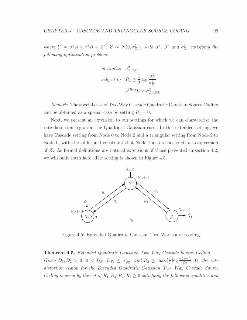
CHAPTER 4. CASCADE AND TRIANGULAR SOURCE CODING 99
where U = α∗A + β∗B + Z∗, Z ∼ N(0, σ2Z∗), with α∗, β∗ and σ2
Z∗ satisfying the
following optimization problem.
maximize σ2A|U,B
subject to R2 ≥1
2log
σ2U
σ2Z∗
22R3D2 ≥ σ2A+B|U
Remark: The special case of TwoWay Cascade Quadratic Gaussian Source Coding
can be obtained as a special case by setting R3 = 0.
Next, we present an extension to our settings for which we can characterize the
rate-distortion region in the Quadratic Gaussian case. In this extended setting, we
have Cascade setting from Node 0 to Node 2 and a triangular setting from Node 2 to
Node 0, with the additional constraint that Node 1 also reconstructs a lossy version
of Z. As formal definitions are natural extensions of those presented in section 4.2,
we will omit them here. The setting is shown in Figure 4.5.
X, Y
Y
Z
R1R2
R3R4
R5
X1, Z1
X2
Z2
Node 0
Node 1
Node 2
Figure 4.5: Extended Quadratic Gaussian Two Way source coding
Theorem 4.5. Extended Quadratic Gaussian Two Way Cascade Source Coding
Given D1, D2 > 0, 0 < DZ1, DZ2 ≤ σ2Z|Y and R2 ≥ max{1
2log
σ2A+σ2
B
D2, 0}, the rate
distortion region for the Extended Quadratic Gaussian Two Way Cascade Source
Coding is given by the set of R1, R3, R4, R5 ≥ 0 satisfying the following equalities and
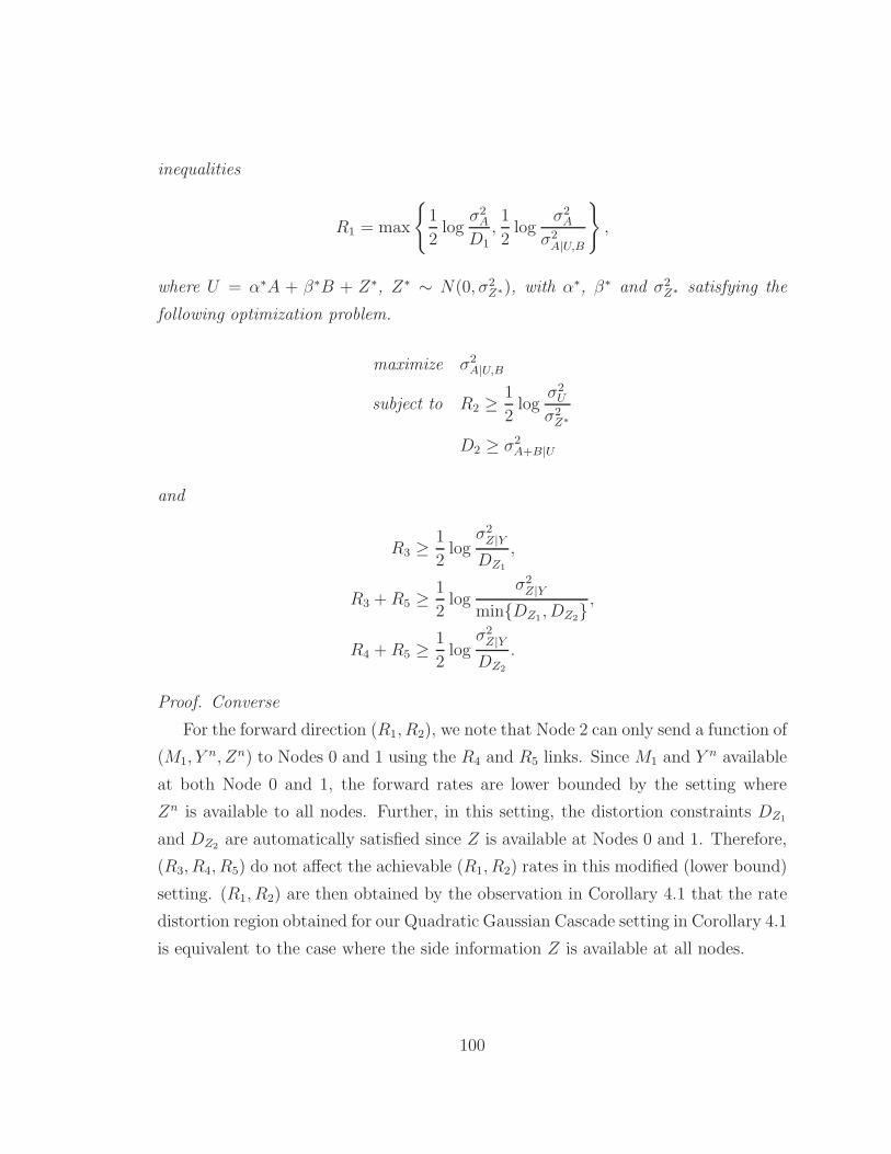
inequalities
R1 = max
{
1
2log
σ2A
D1
,1
2log
σ2A
σ2A|U,B
}
,
where U = α∗A + β∗B + Z∗, Z∗ ∼ N(0, σ2Z∗), with α∗, β∗ and σ2
Z∗ satisfying the
following optimization problem.
maximize σ2A|U,B
subject to R2 ≥1
2log
σ2U
σ2Z∗
D2 ≥ σ2A+B|U
and
R3 ≥1
2log
σ2Z|Y
DZ1
,
R3 +R5 ≥1
2log
σ2Z|Y
min{DZ1 , DZ2},
R4 +R5 ≥1
2log
σ2Z|Y
DZ2
.
Proof. Converse
For the forward direction (R1, R2), we note that Node 2 can only send a function of
(M1, Yn, Zn) to Nodes 0 and 1 using the R4 and R5 links. Since M1 and Y n available
at both Node 0 and 1, the forward rates are lower bounded by the setting where
Zn is available to all nodes. Further, in this setting, the distortion constraints DZ1
and DZ2 are automatically satisfied since Z is available at Nodes 0 and 1. Therefore,
(R3, R4, R5) do not affect the achievable (R1, R2) rates in this modified (lower bound)
setting. (R1, R2) are then obtained by the observation in Corollary 4.1 that the rate
distortion region obtained for our Quadratic Gaussian Cascade setting in Corollary 4.1
is equivalent to the case where the side information Z is available at all nodes.
100
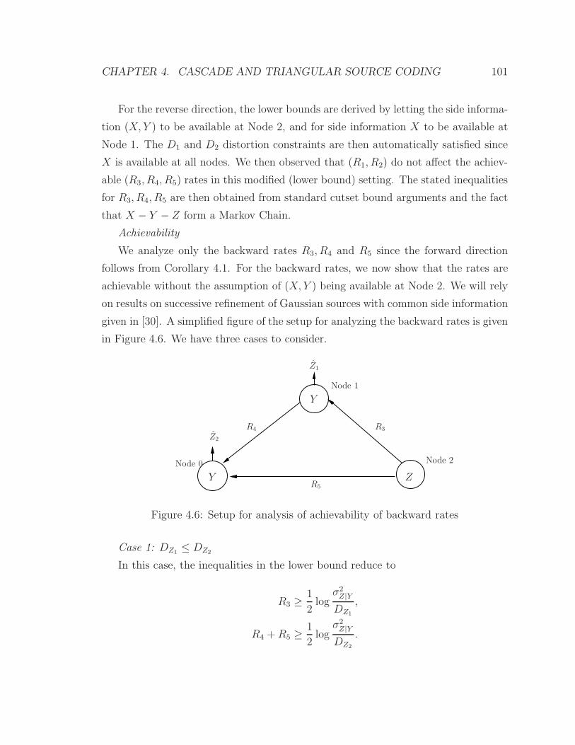
CHAPTER 4. CASCADE AND TRIANGULAR SOURCE CODING 101
For the reverse direction, the lower bounds are derived by letting the side informa-
tion (X, Y ) to be available at Node 2, and for side information X to be available at
Node 1. The D1 and D2 distortion constraints are then automatically satisfied since
X is available at all nodes. We then observed that (R1, R2) do not affect the achiev-
able (R3, R4, R5) rates in this modified (lower bound) setting. The stated inequalities
for R3, R4, R5 are then obtained from standard cutset bound arguments and the fact
that X − Y − Z form a Markov Chain.
Achievability
We analyze only the backward rates R3, R4 and R5 since the forward direction
follows from Corollary 4.1. For the backward rates, we now show that the rates are
achievable without the assumption of (X, Y ) being available at Node 2. We will rely
on results on successive refinement of Gaussian sources with common side information
given in [30]. A simplified figure of the setup for analyzing the backward rates is given
in Figure 4.6. We have three cases to consider.
Y
Y
Z
R3R4
R5
Z1
Z2
Node 0
Node 1
Node 2
Figure 4.6: Setup for analysis of achievability of backward rates
Case 1: DZ1 ≤ DZ2
In this case, the inequalities in the lower bound reduce to
R3 ≥1
2log
σ2Z|Y
DZ1
,
R4 +R5 ≥1
2log
σ2Z|Y
DZ2
.
From the successive refinement results in [30], we can show that the following rates
are achievable
R3 = I(U1, U2, U3;Z|Y ),
R4 = I(U2;Z|Y ),
R5 = I(U3;Z|Y, U2)
for some conditional distribution F (U1, U2, U3|Z), Z1(U1, U2, U3, Y ) and Z2(U1, U2, Y )
satisfying the distortion constraints. Now, for fixed R4 ≤ 12log
σ2Z|Y
DZ2, choose D′(≥
DZ2) such that R4 = 12log
σ2Z|Y
D′ . We now choose the auxiliary random variables and
reconstruction functions in the following manner. Define Q(x) :=xσ2
Z|Y
σ2Z|Y
−x.
U1 = Z +W1 where W1 ∼ N(0, Q(DZ1)),
U3 = U1 +W3 where W3 ∼ N(0, Q(DZ2)−Q(DZ1)),
U2 = U3 +W2 where W2 ∼ N(0, Q(D′)−Q(DZ2)),
Z1 = E(Z|U1, Y ),
Z2 = E(Z|U3, Y ).
From this choice of auxiliary random variables, it is easy to verify the following
R3 = I(U1, U2, U3;Z|Y )
= I(U1;Z|Y )
=1
2log
σ2Z|Y
DZ1
,
R4 = I(U2;Z|Y )
=1
2log
σ2Z|Y
D′,
R4 +R5 = I(U2;Z|Y ) + I(U3;Z|Y, U2)
= I(U3, U2;Z|Y )
102
CHAPTER 4. CASCADE AND TRIANGULAR SOURCE CODING 103
=1
2log
σ2Z|Y
DZ2
,
E(Z − Z1)2 = DZ1 ,
E(Z − Z2)2 = DZ2 .
Case 2: DZ1 > DZ2, R3 ≥ R4
In this case, the active inequalities are
R3 ≥1
2log
σ2Z|Y
DZ1
,
R4 +R5 ≥1
2log
σ2Z|Y
DZ2
.
From [30], the following rates are achievable
R3 = I(U1, U2;Z|Y ),
R4 = I(U2;Z|Y ),
R5 = I(U3, U1;Z|Y, U2).
First, assume R3 ≤ 12log
σ2Z|Y
DZ2. Choose DZ2 ≤ D′ ≤ D′′ ≤ DZ1. We choose the
auxiliary random variables and reconstruction functions as follows.
U3 = Z +W3 where W3 ∼ N(0, Q(DZ2)),
U1 = U3 +W1 where W1 ∼ N(0, Q(D′)−Q(DZ2)),
U2 = U1 +W2 where W2 ∼ N(0, Q(D′′)−Q(D′)),
Z1 = E(Z|U1, Y ),
Z2 = E(Z|U3, Y ).
From this choice of auxiliary random variables, it is easy to verify the following
R3 = I(U1, U2;Z|Y )
= I(U1;Z|Y )
=1
2log
σ2Z|Y
D′,
R4 = I(U2;Z|Y )
=1
2log
σ2Z|Y
D′′,
R4 +R5 = I(U2;Z|Y ) + I(U3, U1;Z|Y, U2)
= I(U3, U1, U2;Z|Y )
= I(U3;Z|Y )
=1
2log
σ2Z|Y
DZ2
,
E(Z − Z1)2 = D′ ≤ DZ1 ,
E(Z − Z2)2 = DZ2.
Next, consider R3 > 12log
σ2Z|Y
DZ2and R4 > 1
2log
σ2Z|Y
DZ2. Then, it is easy to see from
our achievability scheme that we can obtain R′4 < R4, R
′3 < R3 and R5 = 0 by setting
D′ = D′′ = DZ2 . Finally, consider the case where R3 >12log
σ2Z|Y
DZ2and R4 ≤
12log
σ2Z|Y
DZ2.
Then, we observe from our achievability scheme that we can achieve R′3 =
12log
σ2Z|Y
DZ2<
R3 for any R4 and R5 satisfying the inequalities by setting D′ = DZ2.
Case 3: DZ1 > DZ2, R3 < R4
In this case, the active inequalities are
R3 ≥1
2log
σ2Z|Y
DZ1
,
R3 +R5 ≥1
2log
σ2Z|Y
DZ2
.
We first consider the case where R3 ≤ 12log
σ2Z|Y
DZ2. We exhibit a scheme for which
R′4 = R3 (< R4) and still satisfies the constraints. This procedure is done by letting
U2 in case 2 to be equal to U1. For DZ2 ≤ D′ ≤ DZ1, define the auxiliary random
104
CHAPTER 4. CASCADE AND TRIANGULAR SOURCE CODING 105
variables and reconstruction functions as follows.
U3 = Z +W3 where W3 ∼ N(0, Q(DZ2)),
U1 = U3 +W1 where W1 ∼ N(0, Q(D′)−Q(DZ2)),
Z1 = E(Z|U1, Y ),
Z2 = E(Z|U3, Y ).
Then, we have the following.
R3 = I(U1;Z|Y )
=1
2log
σ2Z|Y
D′,
R′4 = I(U1;Z|Y )
=1
2log
σ2Z|Y
D′,
R3 +R5 = I(U1;Z|Y ) + I(U3;Z|Y, U1)
= I(U3, U1;Z|Y )
= I(U3;Z|Y )
=1
2log
σ2Z|Y
DZ2
,
E(Z − Z1)2 = D′ ≤ DZ1 ,
E(Z − Z2)2 = DZ2 .
Finally, we note that in the case where R3 > 12log
σ2Z|Y
DZ2, we can always achieve
R′3 =
12log
σ2Z|Y
DZ2, R′
4 =12log
σ2Z|Y
DZ2and R′
5 = 0 by letting D′ = DZ2 .
Remark 1: The Two-way Cascade source coding setup given in section 4.2 can
be obtained as a special case by setting R3 = R4 = 0 and DZ1 → ∞.
Remark 2: The rate distortion region is the same regardless of whether Node
2 sends first, or Node 0 sends first. This observation follows from (i) our result in
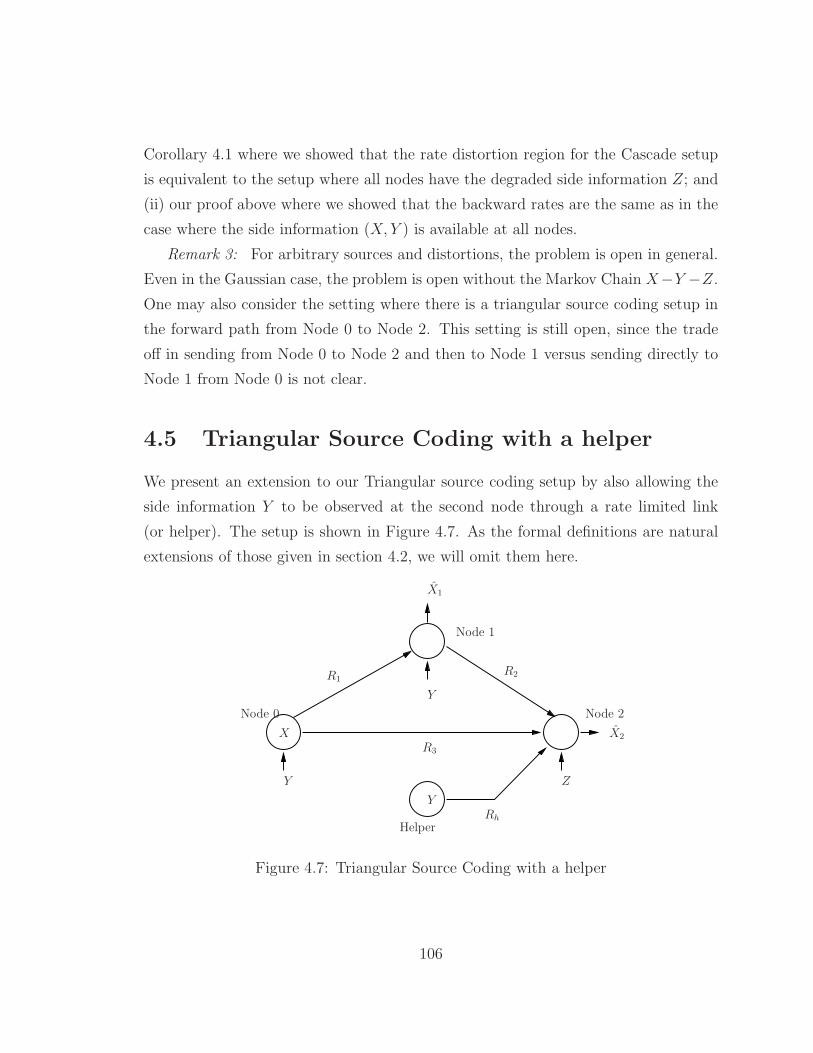
Corollary 4.1 where we showed that the rate distortion region for the Cascade setup
is equivalent to the setup where all nodes have the degraded side information Z; and
(ii) our proof above where we showed that the backward rates are the same as in the
case where the side information (X, Y ) is available at all nodes.
Remark 3: For arbitrary sources and distortions, the problem is open in general.
Even in the Gaussian case, the problem is open without the Markov Chain X−Y −Z.
One may also consider the setting where there is a triangular source coding setup in
the forward path from Node 0 to Node 2. This setting is still open, since the trade
off in sending from Node 0 to Node 2 and then to Node 1 versus sending directly to
Node 1 from Node 0 is not clear.
4.5 Triangular Source Coding with a helper
We present an extension to our Triangular source coding setup by also allowing the
side information Y to be observed at the second node through a rate limited link
(or helper). The setup is shown in Figure 4.7. As the formal definitions are natural
extensions of those given in section 4.2, we will omit them here.
X
Y
Y
Y
Z
R1R2
R3
Rh
X1
X2
Node 0
Node 1
Node 2
Helper
Figure 4.7: Triangular Source Coding with a helper
106
CHAPTER 4. CASCADE AND TRIANGULAR SOURCE CODING 107
Theorem 4.6. The rate distortion region for Triangular source coding with a helper
is given by the set of rate tuples
R1 ≥ I(X ; X1, U1|Y, Uh),
R2 ≥ I(U1;X, Y |Z, Uh),
R3 ≥ I(X, Y ;U2|U1, Uh, Z),
Rh ≥ I(Uh; Y |Z).
for some p(x, y, z, u1, u2, uh, x1) = p(x)p(y|x)p(z|y)p(uh|y)p(u|x, y, uh).
p(x1|x, y, u1, uh)p(u2|x, y, u1, uh) and function g2 : U1 × U2 × Uh × Z → X2 such that
E dj(Xj, Xj) ≤ Dj , j=1,2.
We give a proof of the converse in Appendix C.7. As the achievability techniques
used form a straightforward extension of the techniques described in Appendix C, we
give only a sketch of achievability.
Sketch of Achievability. The achievability follows that of Triangular source coding,
with an additional step of generating a lossy description of Y n. The codebook gener-
ation consists of the following steps
• Generate 2n(I(Y ;Uh)+ǫ) Unh sequences according to
∏ni=1 p(uhi). Partition the set
of Unh sequences into 2n(I(Uh;Y |Z)+2ǫ) bins, Bh(mh), mh ∈ [1 : 2n(I(Uh;Y |Z)+2ǫ)].
• Generate 2n(I(X,Y,Uh;U1)+ǫ) Un1 sequences according to
∏ni=1 p(u1i). Partition the
set of Un1 sequences into 2n(I(U1;X|Y,Uh)+2ǫ) bins, B1(m10). Separately and in-
dependently, partition the set of Un sequences into 2n(I(U1;X,Y |Z,Uh)+2ǫ) bins,
B2(m2), m2 ∈ [1 : 2n(I(U ;X,Y |Z)+2ǫ)].
• For each (un1 , u
nh, y
n) sequence, generate 2n(I(Xn1 ;X|U1,Y,Uh)+ǫ) Xn
1 sequences ac-
cording to∏n
i=1 p(xi|u1i, uhi, yi).
• Generate 2n(I(U2;X,Y |Uh,U1)+ǫ) Un2 sequences according to
∏ni=1 p(u2i|u1i, uhi) for
each (un1 , u
nh) sequence, and partition these sequences to 2n(I(U2;X,Y |U1,Uh,Z)+2ǫ)
bins, B3(m3).
Encoding consists of the following steps
• Helper node: The helper node (and Nodes 0 and 1) looks for a unh sequence such
that (unh, y
n) ∈ T(n)ǫ . This step succeeds with high probability since there are
2n(I(Y ;Uh)+ǫ) Unh sequences. The helper then sends out the bin index mh such
that unh ∈ B(mh). The sequences (un
h, xn, yn, zn) are jointly typical with high
probability due to the Markov Chain (X,Z)− Y − Uh.
• Node 0: Given (xn, yn, unh) ∈ T
(n)ǫ , Node 0 looks for a jointly typical codeword
un1 . This operation succeeds with high probability since there are 2n(I(X,Y,Uh;U1)+ǫ)
Un1 sequences. Node 0 then looks for a xn
1 that is jointly typical with (un1 , x
n, yn, unh).
This operation succeeds with high probability since there are 2n(I(X1;X|U1,Uh,Y )+ǫ)
xn1 sequences.
• Node 0 also finds a un2 sequence that is jointly typical with (un
1 , unh, x
n, yn). This
operation succeeds with high probability since we have 2n(I(U2;X,Y |U1,Uh)+ǫ) vn
sequences.
• Node 0 then sends out the bin index m10 such that un1 ∈ B1(m10) and the index
corresponding to xn1 to Node 1. This requires a total rate of R1 = I(U ;X|Y ) +
I(Xn1 ;X|U, Y ) + 3ǫ to Node 1. Node 0 also sends out the bin index m3 such
that un2 ∈ B(m3) to Node 2. This requires a rate of I(U2;X, Y |U1, Uh, Z) + 2ǫ.
• Node 1 decodes the codeword un1 and forwards the index m2 such that un
1 ∈
B(m2) to Node 2. This requires a rate of I(U1;X, Y |Z, Uh) + 2ǫ.
Decoding consists of the following steps
• Node 1: Node 1 reconstructs un1 by looking for the unique Un
1 sequence in
B1(m10) such that (Un1 , U
nh , Y
n) ∈ T(n)ǫ . Since there are only
2n(I(X,Y,Uh;U1)−I(U1;X|Y,Uh)−ǫ) = 2n(I(U1;Uh,Y )−ǫ) sequences in the bin, this operation
succeeds with high probability. Node 1 reconstructs Xn as Xn1 (m10, m11). Since
the sequence (Xn1 , X
n) are jointly typical with high probability, the expected
distortion constraint is satisfied.
108
CHAPTER 4. CASCADE AND TRIANGULAR SOURCE CODING 109
• Node 2: We note that since (U1, U2, Uh, X)− Y − Z, the sequences
(Unh , U
n1 , U
n2 , X
n, Y n, Zn) are jointly typical with high probability. Decoding at
node 2 consists of the following steps
1. Node 2 first looks for unh in Bh(mh) such that (un
h, zn) ∈ T
(n)ǫ . This op-
eration succeeds with high probability since there are only 2n(I(Uh;Z)−ǫ unh
sequences in the bin.
2. It then looks for un1 in B2(m2) such that (un
h, un1 , z
n) ∈ T(n)ǫ . Since
I(U1;X, Y, Uh) − I(U1;X, Y |Z, Uh) = I(U1;Z, Uh) by the Markov Chain
Z− (X, Y, Uh)−U1, this operation succeeds with high probability as there
are only 2n(I(U1;Z,Uh)−ǫ un1 sequences in the bin.
3. Finally, it looks for un2 in B3(m3) such that (un
h, un1 , u
n2 , z
n) ∈ T(n)ǫ . Since
I(U2;X, Y |Uh, U1)−I(U2;X, Y |Z, Uh, U1) = I(U2;Z|U1, Uh) by the Markov
Chain Z−(X, Y, Uh, U1)−U2, this operation succeeds with high probability
as there are only 2n(I(U2;Z|U1,Uh)−ǫ un2 sequences in the bin.
4. Node 2 then reconstructs using the function x2i = g2(u1i, u2i, uhi, zi) for
i ∈ [1 : n]. Since the sequences (Xn, Zn, Un1 , U
n2 , U
nh ) are jointly typical
with high probability, the expected distortion constraint is satisfied.
4.6 Summary of Chapter
Rate distortion regions for the cascade, triangular, two-way cascade and two-way
triangular source coding settings were established. Decoding part of the description
intended for Node 2 and then re-binning it was shown to be optimum for our Cascade
and Triangular settings. We also extended our Triangular setting to the case where
there is an additional rate constrained helper, which observes Y , for Node 2. In the
Quadratic Gaussian case, we showed that the auxiliary random variables can be taken
to be jointly Gaussian and that the rate-distortion regions obtained for the Cascade
and Triangular setup were equivalent to the setting where the degraded side informa-
tion is available at all nodes. This observation allows us to transform our Cascade

and Triangular settings into equivalent settings for which explicit characterizations
are known. Characterizations of the rate distortion regions for the Quadratic Gaus-
sian cases were also established in the form of tractable low dimensional optimization
programs. Our Two Way Cascade Quadratic Gaussian setting was extended to solve
a more general two way cascade scenario. The case of generally distributed X, Y, Z,
without the degradedness assumption, remains open.
110
Chapter 5
Causal Cascade and Triangular
Source Coding
5.1 Introduction to Cascade and Triangular Source
Coding with causality constraints
This chapter is a continuation of Chapter 4 where we introduced the Cascade and
Triangular Source Coding problems. In that chapter, we characterized the rate-
distortion regions for a variety of settings when the side information at Node 2 is
degraded with respect to the side informations at Nodes 0 and 1. The intuition we
gained from the results and analysis is that the decode and re-bin scheme is usually
optimum when the side information at Node 2 is “poorer” in some sense. This idea
of poorer quality side information was made precise in the previous chapter when we
assumed a Markov condition on the side informations. In this chapter, we will see
another notion of “poorer” quality side information at Node 2 which would allow us
to establish further results for the Cascade and Triangular Source Coding problems.
Therefore, this chapter will focus on other conditions for the Cascade and Trian-
gular settings for which we can establish the rate distortion regions. In this chapter,
we look at the case of causal reconstruction at the end node (Node 2), where Node
2 is constrained to reconstruct the symbol X2i using only the side information from
111
time 1 up to i. This setup of causal source coding (and reconstruction) was first intro-
duced in [34], and motivation for considering this setting can be found in that paper.
Essentially, this problem is motivated by source coding systems that are constrained
to operate with limited or no delay. Source coding systems with encoder and decoder
delay constraints form a subclass of schemes in the setting proposed by [34], since
their setting only imposes delay restrictions on the decoder. Results and bounds in
that paper therefore serve as bounds on the limits of performance for source coding
systems with delay constraints. In [31], this setup was extended to the Gu-Effros
cascade source coding problem [15] when causal reconstruction is required at the end
node.
This chapter also considers the setting of causal reconstruction at the end node,
and we derive more general results for both the cascade and triangular source coding
cases. We begin by providing formal definitions and problem statements in section 5.2.
In section 5.3, we consider the problem of Causal Cascade and Triangular Source
Coding with the same side information Y available at the first 2 nodes (the Source
Node, Node 0, and the intermediate node, Node 1) and side information Z available
at Node 2. We characterize the rate distortion regions for these settings and recover
as a special case, the rate distortion region for the Gu-Effros network. In section 5.4,
we consider the problem of (near) lossless source coding through a cascade with side
informations Y and Z available at Nodes 1 and 2 respectively. We establish the
optimum rate region when the positivity condition [34] p(x, y, z) > 0 for all x, y, z
holds; or when the sources form a Markov chain X − Y − Z.
5.2 Problem Definition
Formal definitions of Causal Cascade and Triangular Source Coding are similar to
the formal definitions given in Chapter 4, but for completeness, and also because we
have are introducing new settings as well, we give the formal definitions for the setups
under consideration in this chapter.
112
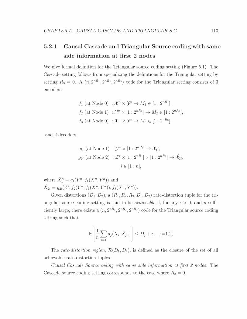
CHAPTER 5. CAUSAL CASCADE AND TRIANGULAR S.C. 113
5.2.1 Causal Cascade and Triangular Source coding with same
side information at first 2 nodes
We give formal definition for the Triangular source coding setting (Figure 5.1). The
Cascade setting follows from specializing the definitions for the Triangular setting by
setting R3 = 0. A (n, 2nR1 , 2nR2, 2nR3) code for the Triangular setting consists of 3
encoders
f1 (at Node 0) : X n ×Yn → M1 ∈ [1 : 2nR1],
f2 (at Node 1) : Yn × [1 : 2nR1] → M2 ∈ [1 : 2nR2 ],
f3 (at Node 0) : X n ×Yn → M3 ∈ [1 : 2nR3],
and 2 decoders
g1 (at Node 1) : Yn × [1 : 2nR1] → X n1 ,
g2i (at Node 2) : Z i × [1 : 2nR2 ]× [1 : 2nR3] → X2i,
i ∈ [1 : n],
where Xn1 = g1(Y
n, f1(Xn, Y n)) and
X2i = g2i(Zi, f2(Y
n, f1(Xn, Y n)), f3(X
n, Y n)).
Given distortions (D1, D2), a (R1, R2, R3, D1, D2) rate-distortion tuple for the tri-
angular source coding setting is said to be achievable if, for any ǫ > 0, and n suffi-
ciently large, there exists a (n, 2nR1 , 2nR2, 2nR3) code for the Triangular source coding
setting such that
E
[
1
n
n∑
i=1
dj(Xi, Xj,i)
]
≤ Dj + ǫ, j=1,2,
The rate-distortion region, R(D1, D2), is defined as the closure of the set of all
achievable rate-distortion tuples.
Causal Cascade Source coding with same side information at first 2 nodes : The
Cascade source coding setting corresponds to the case where R3 = 0.
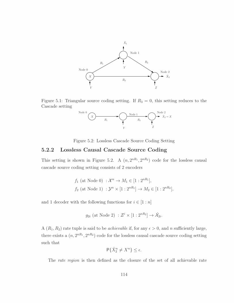
X
Y
Y
Z
R1R2
R3
X1
X2
Node 0
Node 1
Node 2
Figure 5.1: Triangular source coding setting. If R3 = 0, this setting reduces to theCascade setting
X
Y Z
R1 R2
X2 = X
Node 0Node 1
Node 2
Figure 5.2: Lossless Cascade Source Coding Setting
5.2.2 Lossless Causal Cascade Source Coding
This setting is shown in Figure 5.2. A (n, 2nR1, 2nR2) code for the lossless causal
cascade source coding setting consists of 2 encoders
f1 (at Node 0) : X n → M1 ∈ [1 : 2nR1 ],
f2 (at Node 1) : Yn × [1 : 2nR1] → M2 ∈ [1 : 2nR2 ],
and 1 decoder with the following functions for i ∈ [1 : n]
g2i (at Node 2) : Z i × [1 : 2nR2 ] → X2i.
A (R1, R2) rate tuple is said to be achievable if, for any ǫ > 0, and n sufficiently large,
there exists a (n, 2nR1, 2nR2) code for the lossless causal cascade source coding setting
such that
P{Xn2 6= Xn} ≤ ǫ.
The rate region is then defined as the closure of the set of all achievable rate
114
CHAPTER 5. CAUSAL CASCADE AND TRIANGULAR S.C. 115
tuples.
5.3 Causal Cascade and Triangular Source coding
with same side information at first 2 nodes
In this section, we present our results for the first setting described in 5.2.1, which are
single letter characterizations of the rate-distortion regions for both the Triangular
and Cascade Source coding settings. In Theorems 5.1 and 5.2, we will present only
proofs of the converses. The achievability schemes are similar to the schemes presented
in Chapter 4, but with slight modifications to account for the assumption of causal
reconstruction. Due to the similarities, we omit the proof of achievability here and
only mention the two differences that arise in the causal setting:
• In the Causal Cascade setting, Node 2 decodes its intended codeword Un with-
out making use of its side information Zn. Hence, the binning rate at Node 1
has to be higher, which is reflected the rate distortion regions. Similarly, for the
Causal Triangular Source Coding case, Node 2 decodes its intended codewords
V n and Un without making use of the side information Zn.
• At every time i ∈ [1 : n], Node 2 outputs X2i(Un(i), Zi) in the Causal Cascade
case and X2i(Un(i), V n(i), Zi) in the Causal Triangular Source Coding case.
5.3.1 Causal Cascade Source Coding
Theorem 5.1. R(D1, D2) for the Cascade source coding setting defined in section 5.2.1
is given by the set of all rate tuples (R1, R2) satisfying
R1 ≥ I(X ; X1, U |Y ),
R2 ≥ I(U ;X, Y )
for some
p(x, y, z, u, x1) = p(x, y, z)p(u|x, y)p(x1|x, y, u) and function g2 : U × Z → X2 such
that
E dj(X, Xj) ≤ Dj , j=1,2.
The cardinality of U is bounded by |U| ≤ |X ||Y|+ 3.
Remark 1: If Y = X , this setup reduces to the case of causal Wyner-Ziv source
coding discussed in [34].
Remark 2: If Z = ∅, then the case of causal source coding at Node 2 is the same as
noncausal source coding at Node 2. Therefore, Theorem 5.1 reduces to the equivalent
result in [27] when Z = ∅.
Remark 3: Let Y = ∅, X = (X, Y ), d1(X, X1) = d1(X, X) and d2(X, Y ) =
d2(Y , Y ), then we recover the Gu-Effros network [15] with causal source coding at
the end node, which shows that the result in [31] is a special case of Theorem 5.1.
Proof of Converse. Given a
(n, 2nR1, 2nR2) code satisfying the distortion constraints (D1, D2), define Ui =
(X i−1, Y i−1, Z i−1,M2). We have the following.
nR2 ≥ H(M2) = I(Xn, Y n;M2)
=n∑
i=1
I(Xi, Yi;M2|Xi−1, Y i−1)
(a)=
n∑
i=1
(
H(Xi, Yi|Zi−1, X i−1, Y i−1)−H(Xi, Yi|Z
i−1, X i−1, Y i−1,M2))
=n∑
i=1
H(Xi, Yi)−H(Xi, Yi|Ui)
=
n∑
i=1
I(Xi, Yi;Ui).
Step (a) follows from the Markov Chain Z i−1− (X i−1, Y i−1,M2)− (Xi, Yi) which can
be shown by considering
I(Xi, Yi;Zi−1|X i−1, Y i−1,M2) ≤ H(Z i−1|X i−1, Y i−1)−H(Z i−1|Xn, Y n,M2)
116
CHAPTER 5. CAUSAL CASCADE AND TRIANGULAR S.C. 117
= H(Z i−1|X i−1, Y i−1)−H(Z i−1|X i−1, Y i−1) = 0.
Next,
nR1 ≥ H(M1) ≥ H(M1|Yn)
= H(M1,M2|Yn) = I(Xn;M1,M2|Y
n)
=n∑
i=1
I(Xi;M1,M2|Xi−1, Y n)
=
n∑
i=1
(
H(Xi|Yi)−H(Xi|Xi−1, Y n,M1,M2)
)
(a)=
n∑
i=1
(
H(Xi|Yi)−H(Xi|Xi−1, Y n, Z i−1,M1,M2)
)
(b)=
n∑
i=1
(
H(Xi|Yi)−H(Xi|Xi−1, Y n, X1i, Z
i−1,M1,M2))
≥n∑
i=1
H(Xi|Yi)−H(Xi|X1i, Yi, Ui)
=n∑
i=1
I(Xi; X1i, Ui|Yi).
(a) follows from the Markov Chain Z i−1 − (X i−1, Y i−1,M2) − (Xi, Yi) which can
be established using the same technique as that in showing the Markov Chain for
the bound for R2. (b) follows from the fact that X1i is a function of Y n and M1.
Next, the proof is completed in the usual manner by letting Q be a random variable
uniformly distributed over [1 : n] and independent of (Xn, Y n, Zn). We note that
XQ = X , YQ = Y , ZQ = Z and defining U = (UQ, Q) and X1Q = X1 then completes
the proof. The existence of the reconstruction function g2 follows from the definition
of U and the assumption of causal source coding at Node 2. The Markov Chain
(U, X1)− (X, Y )− Z also follows from definitions of U and X1.
5.3.2 Causal Triangular Source Coding
Theorem 5.2. R(D1, D2) for the Triangular source coding setting defined in sec-
tion 5.2.1 is given by the set of all rate tuples (R1, R2, R3) satisfying
R1 ≥ I(X ; X1, U |Y ),
R2 ≥ I(X, Y ;U),
R3 ≥ I(X, Y ;V |U)
for some p(x, y, z, u, v, x1) =
p(x, y, z)p(u|x, y)p(x1|x, y, u)p(v|x, y, u) and function g2 : U ×V ×Z → X2 such that
E dj(X, Xj) ≤ Dj , j=1,2.
The cardinalities for the auxiliary random variables can be upper bounded by |U| ≤
|X ||Y|+ 4 and |V| ≤ (|X ||Y|+ 4)(|X ||Y|+ 1).
Similar to the Cascade case, if Z = ∅, this region reduces to the Triangular source
coding region given in [27].
Proof of Converse. The converse is proved in two parts. In the first part, the re-
quired inequalities are derived and in the second part, we need to show that the joint
probability distribution can be restricted to the form stated in the Theorem. Proof
for the first part is given, while for the second part, the proof follows similar lines to
a technique in [27, Lemma 5] and we refer readers to it.
Given a (n, 2nR1, 2nR2 , 2nR3) code satisfying the distortion constraints (D1, D2),
define Ui = (X i−1, Y i−1, Z i−1,M2) and Vi = M3. We omit proof of the R1 and R2
inequalities since it follows the same steps as in Theorem 5.1. For R3, we have
nR3 ≥ H(M3) ≥ I(Xn, Y n;M3|M2)
(a)=
n∑
i=1
(
H(Xi, Yi|M2, Xi−1, Y i−1)−H(Xi, Yi|M2,M3, X
i−1, Y i−1, Z i−1))
118
CHAPTER 5. CAUSAL CASCADE AND TRIANGULAR S.C. 119
≥n∑
i=1
H(Xi, Yi|Ui)−H(Xi, Yi|Ui, Vi)
=
n∑
i=1
I(Xi, Yi;Vi|Ui).
(a) follows from the Markov Chain Z i−1 − (M2,M3, Xi−1, Y i−1) − (Xi, Yi). Now,
let Q be a random variable uniformly distributed over [1 : n] and independent of
(Xn, Y n, Zn). We then obtain the bounds stated in Theorem 5.2 by defining U =
(UQ, Q), V = (VQ, Q) and X1Q = X1. The existence of the reconstruction function
g2i for i ∈ [1 : n] follows from the definition of U , V and the assumption of causal
reconstruction. Next, from the definitions of U , V and X1, we note the following
Markov relation: (U, V, X1) − (X, Y ) − Z. The joint probability distribution can
then be factored as p(x, y, z, u, v, x1) = p(x, y, z)p(u|x, y)p(x1, v|x, y, u). Proof of this
second part is omitted here.
5.4 Lossless Causal Cascade Source Coding
In this section, we present results for the setting described in 5.2.2. The case when a
positivity condition is satisfied is presented in Theorem 5.3, while the case ofX−Y −Z
forming a Markov Chain is presented in Theorem 5.4.
Theorem 5.3. Let p(x, y, z) > 0 for all x ∈ X , y ∈ Y , z ∈ Z. Then, the rate region
for lossless cascade source coding setting defined in section 5.2.2 is given by the set
of (R1, R2) satisfying
R1 ≥ H(X|Y ),
R2 ≥ H(X).
Remark: This result extends the result in [34]. It shows that the side information
at the end node does not help when the positivity condition holds. Xn has to be
communicated to both Node 1 and Node 2, without the use of side information Zn.
It is clear that we can generalize this theorem slightly by requiring lossy reconstruction
at the Node 1. The rate region remains unchanged as R1 ≥ H(X|Y ) implies that we
can satisfy the distortion constraint since Xn is recovered (near) losslessly at Node 1.
Proof: We give a proof of converse, since the achievability is straightforward. The
converse follows from cutset bound arguments. We first obtain a lower bound on
R1 by cutset arguments and relaxing the lossless requirement to Hamming distortion
with D ≥ 0. Let X2i be a function of M1, Yn, Z i and the distortion measure be
Hamming distortion. Then, defining Ui = (Y n/i, Z i−1,M1), we have
R1(D) ≥ H(M1) ≥ I(M1;Xn|Y n)
=
n∑
i=1
H(Xi|Yi)−H(Xi|Xi−1, Y n,M1)
=n∑
i=1
H(Xi|Yi)−H(Xi|Xi−1, Y n, Z i−1,M1)
≥n∑
i=1
I(Xi;Ui|Yi).
(a) follows from the Markov Chain Z i−1 − (X i−1, Y n,M1)−Xi. The lower bound is
then obtained following standard procedures and the observation that U−X−(Y, Z).
We have
R1(D) ≥ minU−X−(Y,Z):E d(X,X2(U,Y,Z))≤D
I(X ;U |Y ).
Setting D = 0 and following the procedure in [34], we can show that the lower bound
reduces to
R1 ≥ minU−X−(Y,Z):H(X|U,Y,Z)=0
I(X ;U |Y ).
We now show that the above expression is lower bounded by H(X|Y ), thereby giving
us the required lower bound for R1. To show this, first take (u, x) such that p(u|x) > 0
and p(u) > 0. We note that such a pair always exists since p(x) > 0 from positivity
condition and p(u) =∑
x p(x)p(u|x) > 0. Now, we show that p(u|x′) = 0 for all
x′ 6= x.
120
CHAPTER 5. CAUSAL CASCADE AND TRIANGULAR S.C. 121
First, note that since p(u) > 0, there exists (y, z) such that p(u, y, z) > 0. But
since H(X|U, Y, Z) = 0, we must have H(X|U = u, Y = y, Z = z) = 0. Hence,
p(x|u, y, z) is either 0 or 1. But since p(x|u, y, z) ≥ p(x, u, y, z) = p(x, y, z)p(u|x) > 0
by positivity condition, we have p(x|u, y, z) = 1 and hence, p(x′|u, y, z) = 0. Since
p(x′|u, y, z) ≥ p(x′, u, y, z) = p(x′, y, z)p(u|x′) = 0 and p(x′, y, z) > 0, p(u|x′) = 0 for
all x′ 6= x. Therefore, p(x|u) = 1 for every u such that p(u) > 0 and some x ∈ X .
This result implies that
H(X|Y, U) ≤ H(X|U)
=∑
u
p(u)H(X|U = u) = 0.
Hence, R1 ≥ minU−X−(Y,Z):H(X|U,Y,Z)=0 I(X ;U |Y ) ≥ H(X|Y ).
Lower Bound on R2
We now turn to proving the required lower bound for R2.
Proof. From cutset argument and following similar procedure as that for R1, we can
show the following lower bound for R2,
R2 ≥ minU−(X,Y )−Z:H(X|Z,U)=0
I(X, Y ;U).
The auxiliary U used in the lower bound can be taken as U = (UQ, Q), where UQ =
(ZQ−1,M2) and Q is a random variable uniformly distributed over [1 : n], independent
of other random variables. We now show that this expression is lower bounded by
H(X) following similar arguments to that forR1. Take (u, x) such that p(u|x) > 0 and
p(u) > 0 as before. Since p(u) > 0, there exists at least one z such that p(u, z) > 0.
Hence, we have H(X|U = u, Z = z) = 0 from the condition that H(X|U,Z) =
0. Therefore, p(x|z, u) is either 0 or 1. Next, we have p(x|u, z) ≥ p(x, u, z) =∑
y p(x, y, z, u) =∑
y p(x, y, z)p(u|x, y). Now, since p(y|x) > 0 for all (x, y) and
p(u|x) =∑
y p(y|x)p(u|x, y) > 0, there must exist a y such that p(u|x, y) > 0. Hence,
p(x|u, z) > 0 from p(u|x, y) > 0 and p(x, y, z) > 0, which implies that p(x|u, z) = 1
and p(x′|u, z) = 0 for x′ 6= x.
Since p(x′|u, z) ≥ p(x′, u, z) =∑
y p(x′, y, z)p(u|x′, y) = 0 and p(x′, y, z) > 0 for
all y by positivity, we have that p(u|x′, y) = 0 for all y, which implies that p(u|x′) =∑
y p(y|x′)p(u|x′, y) = 0. We therefore have p(u) =
∑
x′′ p(x′′)p(u|x′′) = p(u, x).
Hence, p(x|u) = 1 for some x ∈ X and every u such that p(u) > 0. Finally, the proof
is completed by observing that
minU−(X,Y )−Z:H(X|U,Z)=0
I(X, Y ;U) ≥ minU−(X,Y )−Z:H(X|U,Z)=0
H(X)−H(X|U)
= H(X).
Theorem 5.4 (Markov chain X − Y − Z). For the
lossless cascade source coding setting defined in section 5.2.2, if X − Y − Z form a
Markov chain, then the rate region for lossless causal source coding is given by
R1 ≥ H(X|Y ),
R2 ≥ I(X, Y ;U)
for some p(u|x, y) such that H(X|U,Z) = 0.
Remark: Unlike the case when noncausal side information Zn is available at the
end node, the case of X − Z − Y forming a Markov Chain is, to the best of our
knowledge, still open for the case of causal reconstruction at the end node.
Achievability sketch: Fix p(u|x, y) such that H(X|U,Z) = 0. We first describe
Xn to Node 1, which can be done using a rate of H(X|Y )+ δ1(ǫ). Node 1 then codes
for the end node using a lossy source code with Hamming distortion and distortion,
D = 0. Node 1 carries out this step out by covering (Xn, Y n) with Un, which requires
a rate of I(U ;X, Y ) + δ2(ǫ). Node 2 then reconstructs Xi by X2i = g2i(Ui, Zi). It
remains to show that this procedure yields a code with vanishing block probability
of error. First, consider (xn, zn, un(m2)) ∈ T(n)ǫ . Then, pX,Z,U(xi, zi, ui) > 0 for all
i ∈ [1 : n]. From the condition H(X|U,Z) = 0, we see that xi(ui, zi) = xi for
i ∈ [1 : n]. Next, let 0 < ǫ′ < ǫ and define the following error events
P(E1) := P((Xn, Y n) /∈ T(n)ǫ′ ),
122
CHAPTER 5. CAUSAL CASCADE AND TRIANGULAR S.C. 123
P(E2) := P(Xn1 (Y
n) 6= Xn) (at Node 1),
P(E3) := P((Un(M2), Xn1 , Y
n, Zn) /∈ T (n)ǫ ).
Then, the probability of “error” is upper bounded by
P(E) ≤ P(E1) + P(E2 ∩ E c1) + P(E3 ∩ (E2 ∪ E1)
c).
P(E1) → 0 as n → ∞ by law of large numbers; P(E2 ∩ E c1) → 0 as n → ∞ since R1 =
H(X|Y )+δ1(ǫ) and P(E3∩(E2∪E1)c) → 0 as n → ∞ because R2 = I(U ;X, Y )+δ2(ǫ)
and by the conditional typicality lemma [13, Lecture 2], since U − (X, Y )− Z.
On E c, note that Xn1 = Xn and (Un(M2), X
n1 , Z
n) = (Un(M2), Xn, Zn) ∈ T (n)
ǫ .
Hence,
P(Xn2 6= Xn|E c) = 0,
which implies that P(Xn2 6= Xn) ≤ P(E). Since P(E) → 0 as n → ∞, this establishes
the achievability of the rate region.
Converse Sketch: As the proof of converse for this case is relatively straightforward
and is similar to that in Theorem 5.3, we give only a sketch.
The lower bound for R1 is established using straightforward cutset arguments and
the Markov Chain assumption X − Y − Z:
Given a (n, 2nR1, 2nR2) code, we have
nR1 ≥ H(M1)
= I(M ;Xn)
≥ I(Xn;M |Y n, Zn)
(a)= H(Xn|Y n, Zn)−H(Xn|Y n,M1,M2, Z
n)
(b)
≥ H(Xn|Y n, Zn)− nǫn
(c)= nH(X|Y )− nǫn.
(a) follows fromM2 being a function of Y n,M1; (b) follows from Fano’s inequality and
the assumption of vanishing block error probability at Node 2; (c) follows from the
i.i.d nature of the source and the side information, and the Markov Chain X−Y −Z.
The lower bound for R2 is established using procedures similar to those used in
establishing the lower bounds for R1 and R2 in Theorem 5.3. We therefore omit the
proof here.
5.5 Summary of Chapter
In this chapter, we considered the cascade and triangular source coding with side
information and causal reconstruction at the end node. When the side information at
the source and intermediate nodes are the same, we characterized the rate distortion
regions for both the cascade and triangular source coding problems. For the cascade
setting with causal lossless reconstruction at the end node, we characterized the rate
region when the sources satisfy a positivity condition, or when a Markov chain holds.
124
Chapter 6
Conclusions
In this thesis, we discussed two sub-areas in Network Information Theory and pre-
sented results for both these areas: Information-Theoretic Secrecy and Multi-terminal
Source Coding.
In the area of Information-Theoretic Secrecy, we looked at two generalizations of
the Wiretap Channel. We first generalized the wiretap channel to more than one
legitimate receiver and to more than one eavesdropper. Inner bounds were given for
the various settings considered and were shown to be optimum for several classes of
three receivers wiretap channels. An interesting idea developed in the inner bounds
was the idea of structured noise generation, where we generate secrecy through a
publicly available superposition codebook. We then looked at a generalization of the
wiretap channel to a wiretap channel with state setup, where both the sender and the
legitimate receiver has access to the channel state information causally. We developed
a new inner bound to the secrecy capacity for this setting and showed that the inner
bound can be strictly larger than previously developed inner bound, which also uses
the more restrictive assumption of noncausal state information at the sender. The
main idea (and difference) in our inner bound is to use the state information as a key
in a block Markov setting to increase the secret message transmission rate.
The second part of the thesis deals with the Cascade and Triangular Source Coding
problem, where we first characterized the rate-distortion regions for both the Cascade
and Triangular Source Coding under an assumption on the statistical structure of the
125

source and side informations. Specifically, we showed that when we have the same side
information at the source node and the intermediate node, and a degraded version
of the side information at the end node, an optimal coding scheme is the decode and
re-bin coding scheme, where, at the intermediate node, we decode the codeword that
was meant for the end node and re-bin it to reduce the transmission rate. We then
extended our analysis to several other related settings. Next, motivated by the idea
that the decode and re-bin scheme is usually optimum when the side information at
Node 2 is poorer in some sense, we consider the Cascade and Triangular Source Coding
problem when we restrict the reconstruction at the end node to causal reconstruction.
When the side information at the source and intermediate nodes are the same, we
characterized the rate distortion regions for both the cascade and triangular source
coding problems, without the degradedness assumption. For the cascade setting with
causal lossless reconstruction at the end node, we characterized the rate region when
the sources satisfy a positivity condition, or when a Markov chain holds.
126
Appendix A
Proofs for Chapter 2
A.1 Proof of Lemma 2.1
First, define N(Un, Zn) = |{k ∈ [1 : 2nS] : (Un, V n(k), Zn) ∈ T(n)ǫ }|. Next, we
define the following “error” events. Let E1(Un, Zn) = 1 if {N(Un, Zn) ≥ (1 +
δ1(ǫ))2n(S−I(V ;Z|U)+δ(ǫ))} and E1 = 0 otherwise. Let E = 0 if (Un, V n(L), Zn) ∈ T
(n)ǫ
and E1(Un, Zn, L) = 0, and E = 1 otherwise. We now show that if S ≥ I(V ;Z|U) +
δ(ǫ), then P{E = 1} → 0 as n → ∞. By the union of events bound,
P{E = 1} ≤ P{(Un, V n(L), Zn) /∈ T (n)ǫ }+ P{E1(U
n, Zn, L) = 1}.
The first term tends to zero as n → ∞ by assumption. The second term is bounded
as follows. Define A(un, zn) as the event (E1(un, Zn) = 1) ∩ (Zn = zn)
P{E1(Un, Zn) = 1} =
∑
un∈T(n)ǫ
p(un)P{(E1(Un, Zn) = 1)|Un = un}
=∑
un∈T(n)ǫ
∑
zn∈T(n)ǫ (Z|U)
p(un)P{An(un, zn)|Un = un}
≤∑
un∈T(n)ǫ
p(un).
(
∑
zn∈T(n)ǫ (Z|U)
P{(E1(un, zn) = 1)|Un = un}
)
.
127
Now, P{E1(un, zn) = 1|Un = un} = P{N(un, zn) ≥ (1 + δ1(ǫ))2
n(S−I(V ;Z|U)+δ(ǫ))|Un =
un}. Define Xk = 1 if (un, V n(k), zn) ∈ T(n)ǫ and 0, otherwise. We note that Xk,
k ∈ [1 : 2nS], are i.i.d. Bernoulli p random variables, where 2−n(I(V ;Z|U)+δ(ǫ)) ≤ p ≤
2−n(I(V ;Z|U)−δ(ǫ)). We have
P
{(
N(un, zn)
≥ (1 + δ1(ǫ))2n(S−I(V ;Z|U)+δ(ǫ))
)
| Un = un
}
≤ P
2nS∑
k=1
Xk ≥ (1 + δ1(ǫ))2nSp
|Un = un
.
Applying the Chernoff Bound (e.g., see [13, Appendix B]), we have
P
2nS∑
k=1
Xk ≥ (1 + δ1(ǫ))2nSp|Un = un
≤ exp(−2nSpδ21(ǫ)/4)
≤ exp(−2n(S−I(V ;Z|U)−δ(ǫ))δ21(ǫ)/4).
Hence,
P{E1(Un, Zn) = 1} ≤
∑
un∈T(n)ǫ
p(un).
(
∑
zn∈T(n)ǫ (Z|U)
exp(−2n(S−I(V ;Z|U)−δ(ǫ))δ21(ǫ)/4)
)
≤ 2n log |Z| exp(−2n(S−I(V ;Z|U)−δ(ǫ))δ21(ǫ)/4),
which tends to zero as n → ∞ if S > I(V ;Z|U) + δ(ǫ).
We are now ready to bound H(L|C, Zn, Un). Consider
H(L,E|C, Un, Zn) ≤ 1 + P{E = 1}H(L|C, E = 1, Un, Zn)
+ P{E = 0}H(L|C, E = 0, Un, Zn)
≤ 1 + P{E = 1}nS + log((1 + δ1(ǫ))2n(S−I(V ;Z|U)+δ(ǫ)))
≤ n(S − I(V ;Z|U) + δ′(ǫ)).
This completes the proof of the lemma.
128
APPENDIX A. PROOFS FOR CHAPTER 2 129
A.2 Evaluation for example
We first give an upper bound for the extended Csiszar–Korner lower bound.
Fact : The extended Csiszar and Korner lower bound in (2.6) for the channel
shown in Figure 2.2 is upper bounded by
RCK ≤ min {I(X1; Y11)− I(X1;Z1) + I(V2; Y12|Q2)− I(V2;Z2|Q2), I(X1; Y21)
−I(X1;Z1)− I(V2;Z2|Q2)} .
for some p(x1)p(q2, v2)p(x2|v2).
Proof. From (2.6), we have
R ≤ maxp(q)p(v|q)p(x|v)
min {I(V ; Y1|Q)− I(V ;Z|Q), I(V ; Y2|Q)− I(V ;Z|Q)} .
Consider the first bound for RCK.
I(V ; Y1|Q)− I(V ;Z|Q) = I(V ; Y11, Y12|Q)− I(V ;Z1|Q)− I(V ;Z2|Q,Z1)
≤ I(V ; Y11, Y12, Z1|Q)− I(V ;Z1|Q)− I(V ;Z2|Q,Z1)
= I(V ; Y11, Y12|Q,Z1)− I(V ;Z2|Q,Z1)
= I(V ; Y11|Q,Z1, Y12) + I(V ; Y12|Q,Z1)− I(V ;Z2|Q,Z1)
= I(V ; Y11, Z1|Q, Y12)− I(V ;Z1|Q, Y12) + I(V ; Y12|Q,Z1)
− I(V ;Z2|Q,Z1)
(a)= I(V ; Y11|Q, Y12)− I(V ;Z1|Q, Y12) + I(V ; Y12|Q,Z1)
− I(V ;Z2|Q,Z1)
≤ I(V ′; Y11|Q)− I(V ′;Z1|Q) + I(V ; Y12|Q,Z1)
− I(V ;Z2|Q,Z1).
(a) follows from the structure of the channel which gives the Markov condition
(Q, Y12, V )− Y11 − Z1. The last step follows from defining V ′ = (V, Y12) and the fact
that Z1 is a degraded version of Y11.
Consider now the second bound.
RCK ≤ I(V ; Y2|Q)− I(V ;Z|Q)
= I(V ; Y21|Q)− I(V ;Z1|Q)− I(V ;Z2|Q,Z1)
≤ I(V ′; Y21|Q)− I(V ′;Z1|Q)− I(V ;Z2|Q,Z1).
Combining the bounds, we have
RCK ≤ min {I(V ′; Y11|Q)− I(V ′;Z1|Q) + I(V ; Y12|Q,Z1)− I(V ;Z2|Q,Z1), (A.1)
I(V ′; Y21|Q)− I(V ′;Z1|Q)− I(V ;Z2|Q,Z1)}
for some p(q)p(v|q)p(x1, x2|v). Now, we note that the terms I(V ′; Y11|Q)−I(V ′;Z1|Q)
and I(V ′; Y21|Q)− I(V ′;Z1|Q) depends only on the marginal distribution
p(q)p(v′|q)p(x1|v′)p(y21, y11, z1|x1). Similarly, defineQ′ = (Q,Z1), the terms I(V ; Y12|Q
′)−
I(V ;Z2|Q′) and I(V ;Z2|Q
′) depends only on the marginal distribution
p(q′, v, x2)p(y12, z2|x2). Therefore, we can further upper bound RCK by
RCK ≤ maxmin {I(V1; Y11|Q1)− I(V1;Z1|Q1) + I(V2; Y12|Q2)− I(V2;Z2|Q2),
I(V1; Y21|Q1)− I(V1;Z1|Q1)− I(V2;Z2|Q2)} ,
where the maximum is over p(q1)p(v1|q1)p(x1|v1) and p(q2)p(v2|q2)p(x2|v2)1. We now
further simplify this bound as follows.
RCK ≤ maxmin {I(V1; Y11|Q1)− I(V1;Z1|Q1) + I(V2; Y12|Q2)− I(V2;Z2|Q2),
I(V1; Y21|Q1)− I(V1;Z1|Q1)− I(V2;Z2|Q2)} ,
≤ maxmin {I(X1; Y11)− I(X1;Z1) + I(V2; Y12|Q2)− I(V2;Z2|Q2),
I(X1; Y21)− I(X1;Z1)− I(V2;Z2|Q2)} ,
where the maximum is now over distributions of the form p(x1) and p(q2)p(v2|q2)p(x2|v2).
1To see that this bound is at least as large as the previous bound in (A.1), set V1 = V ′, Q1 = Q,V2 = (V,Q′) and Q2 = Q′ in this bound to recover the previous bound
130
APPENDIX A. PROOFS FOR CHAPTER 2 131
The last step follows from the fact that Z1 is degraded with respect to both Y21 and
Y11.
Next, we evaluate this upper bound. We will make use of the entropy relation-
ship [6]: H(ap, 1− p, (1− a)p) = H(p, 1− p) + pH(a, 1− a). First consider the terms
for the first channel components,
(I(X1; Y11) − I(X1;Z1)) and (I(X1; Y21) − I(X1;Z1)). Letting P{X1 = 0} = γ and
evaluating the individual expressions, we obtain
I(X1; Y21) = H(γ, 1− γ),
I(X1; Y11) = H
(
γ
2,1
2,1− γ
2
)
− 1
=1
2H(γ, 1− γ),
I(X1;Z1) = H
(
γ
6,5
6,5(1− γ)
6
)
−H
(
1
6,5
6
)
=1
6H(γ, 1− γ).
This gives
I(X1; Y21)− I(X1;Z1) =5
6H(γ, 1− γ),
I(X1; Y11)− I(X1;Z1) =1
3H(γ, 1− γ).
Note that both expressions are maximized by setting γ = 1/2, which yields
RCK ≤ min
{
1
3+ I(V2; Y12|Q2)− I(V2;Z2|Q2),
5
6− I(V2;Z2|Q2)
}
. (A.2)
Next, we consider the second channel component terms. Let αi = p(q2i), βj,i =
p(v2j |q2i), P{X2 = 0|V2 = v2j} = µj, and P{V2 = v2j} = νj , then
I(V2;Z2|Q2) =∑
i
αiH
(
∑
j βj,iµj
2,1
2,
∑
j βj,i(1− µj)
2
)
−∑
j
νjH
(
µj
2,1
2,(1− µj)
2
)
=1
2
∑
i
αiH
(
∑
j
βj,iµj,∑
j
βj,i(1− µj)
)
−1
2
∑
j
νjH (µj, (1− µj)) ,
I(V2; Y12|Q2) =∑
i
αiH
(
∑
j
βj,iµj,∑
j
βj,i(1− µj)
)
−∑
j
νjH (µj , (1− µj)) .
This implies that
I(V2; Y12|Q2)− I(V2;Z2|Q2) =1
2
∑
i
αiH
(
∑
j
βj,iµj ,∑
j
βj,i(1− µj)
)
−1
2
∑
j
νjH (µj, (1− µj)) .
Comparing the above expressions, we see that I(V2;Z2|Q2) = 0 implies that I(V2; Y12|Q2)−
I(V2;Z2|Q2) = 0. This, together with (A.2), implies that RCK is strictly less than
5/6.
In comparison, consider the new lower bound in Corollary 2.1. Setting V = X1
and X1 and X2 independent Bernoulli 1/2, we have
I(X1, X2; Y11, Y12)− I(X1, X2;Z1, Z2) = I(X1; Y11)− I(X1;Z1) + I(X2; Y12)− I(X2;Z2)
=1
3+
1
2=
5
6,
I(V ; Y2)− I(V ;Z) = I(X1; Y21)− I(X1;Z1, Z2)
= I(X1; Y21)− I(X1;Z1)
=5
6.
Thus, R = 5/6 is achievable using the new scheme, which shows that the our lower
bound can be strictly larger than the extended Csiszar and Korner lower bound. In
fact, R = 5/6 is the capacity for this example since the channel is a special case of the
reversely degraded broadcast channel considered in [18] and we can use the converse
result therein to show that CS ≤ 5/6.
132
APPENDIX A. PROOFS FOR CHAPTER 2 133
A.3 Proof of Theorem 2.2
Using Fourier–Motzkin elimination on the rate constraints gives the following region.
R0 < I(U ;Z),
R1 < min {I(V0, V1; Y1|U)− I(V1;Z|V0), I(V0, V2; Y2|U)− I(V2;Z|V0)} ,
2R1 < I(V0, V1; Y1|U) + I(V0, V2; Y2|U)− I(V1;V2|V0), (A.3)
R0 +R1 < min {I(V0, V1; Y1)− I(V1;Z|V0), I(V0, V2; Y2)− I(V2;Z|V0)} ,
R0 + 2R1 < I(V0, V1; Y1) + I(V0, V2; Y2|U)− I(V1;V2|V0), (A.4)
R0 + 2R1 < I(V0, V2; Y2) + I(V0, V1; Y1|U)− I(V1;V2|V0), (A.5)
2R0 + 2R1 < I(V0, V1; Y1) + I(V0, V2; Y2)− I(V1;V2|V0), (A.6)
Re ≤ R1,
Re < min {I(V0, V1; Y1|U)− I(V0, V1;Z|U), I(V0, V2; Y2|U)− I(V0, V2;Z|U)} ,
2Re < I(V0, V1; Y1|U) + I(V0, V2; Y2|U)− I(V1;V2|V0)− 2I(V0;Z|U), (A.7)
R0 +Re < min {I(V0, V1; Y1)− I(V1, V0;Z|U), I(V0, V2; Y2)− I(V2, V0;Z|U)} ,
R0 + 2Re < I(V0, V1; Y1) + I(V0, V2; Y2|U)− I(V1;V2|V0)− 2I(V0;Z|U),
R0 + 2Re < I(V0, V2; Y2) + I(V0, V1; Y1|U)− I(V1;V2|V0)− 2I(V0;Z|U),
2R0 + 2Re < I(V0, V1; Y1) + I(V0, V2; Y2)− I(V1;V2|V0)− 2I(V0;Z|U), (A.8)
with the constraint of I(V1, V2;Z|V0) ≤ I(V1;Z|V0) + I(V2;Z|V0) − I(V1;V2|V0) on
the set of possible probability distributions. Due to this constraint, the numbered
inequalities in the above region are redundant.
We now complete the proof by using rate splitting. This is equivalent to letting
R1 = R′′1 , R0 = Rn
0 +R′1 in the above region and letting the new rates be Rn
0 for the
common message and Rn1 = R′
1+R′′11 for the private message. Using Fourier-Motzkin
to eliminate the auxiliary rates R′1 and R′′
1 then results in the following region.
R0 < I(U ;Z),
R0 +R1 < I(U ;Z) + min {I(V0, V1; Y1|U)− I(V1;Z|V0),
I(V0, V2; Y2|U)− I(V2;Z|V0)} ,
R0 +R1 < min {I(V0, V1; Y1)− I(V1;Z|V0), I(V0, V2; Y2)− I(V2;Z|V0)} ,
Re ≤ R1,
Re < min {I(V0, V1; Y1|U)− I(V0, V1;Z|U), I(V0, V2; Y2|U)− I(V0, V2;Z|U)} ,
R0 +Re < min {I(V0, V1; Y1)− I(V1, V0;Z|U), I(V0, V2; Y2)− I(V2, V0;Z|U)} ,
R0 + 2Re < I(V0, V1; Y1) + I(V0, V2; Y2|U)− I(V1;V2|V0)− 2I(V0;Z|U),
R0 + 2Re < I(V0, V2; Y2) + I(V0, V1; Y1|U)− I(V1;V2|V0)− 2I(V0;Z|U),
R0 +R1 +Re < min {I(V0, V1; Y1|U)− I(V1;Z|V0), I(V0, V2; Y2|U)− I(V2;Z|V0)}
+min {I(V0, V1; Y1)− I(V1, V0;Z|U), I(V0, V2; Y2)− I(V2, V0;Z|U)} ,
R0 +R1 + 2Re < min {I(V0, V1; Y1|U)− I(V1;Z|V0), I(V0, V2; Y2|U)− I(V2;Z|V0)}
+ I(V0, V1; Y1) + I(V0, V2; Y2|U)
− I(V1;V2|V0)− 2I(V0;Z|U),
R0 +R1 + 2Re < min {I(V0, V1; Y1|U)− I(V1;Z|V0), I(V0, V2; Y2|U)− I(V2;Z|V0)}
+ I(V0, V2; Y2) + I(V0, V1; Y1|U)− I(V1;V2|V0)− 2I(V0;Z|U).
Eliminating redundant inequalities then results in
R0 < I(U ;Z),
R0 +R1 < I(U ;Z) + min {I(V0, V1; Y1|U)− I(V1;Z|V0),
I(V0, V2; Y2|U)− I(V2;Z|V0)} ,
R0 +R1 < min {I(V0, V1; Y1)− I(V1;Z|V0), I(V0, V2; Y2)− I(V2;Z|V0)} ,
Re ≤ R1,
Re < min {I(V0, V1; Y1|U)− I(V0, V1;Z|U), I(V0, V2; Y2|U)− I(V0, V2;Z|U)} ,
134
APPENDIX A. PROOFS FOR CHAPTER 2 135
R0 +Re < min {I(V0, V1; Y1)− I(V1, V0;Z|U), I(V0, V2; Y2)− I(V2, V0;Z|U)} ,
R0 + 2Re < I(V0, V1; Y1) + I(V0, V2; Y2|U)− I(V1;V2|V0)− 2I(V0;Z|U),
R0 + 2Re < I(V0, V2; Y2) + I(V0, V1; Y1|U)− I(V1;V2|V0)− 2I(V0;Z|U),
R0 +R1 + 2Re < I(V0, V2; Y2|U)− I(V2;Z|V0) + I(V0, V1; Y1) + I(V0, V2; Y2|U)
− I(V1;V2|V0)− 2I(V0;Z|U),
R0 +R1 + 2Re < I(V0, V1; Y1|U)− I(V1;Z|V0) + I(V0, V2; Y2) + I(V0, V1; Y1|U)
− I(V1;V2|V0)− 2I(V0;Z|U).
A.4 Converse for Proposition 2.2
The R1 inequalities follow from a technique used in [26, Proposition 11]. We provide
the proof here for completeness.
nR1 ≤∑
i
I(M1; Y1i|M0, Yn1,i+1) + nǫn
≤∑
i
I(M1; Y1i|M0, Yn1,i+1, Z
i−1) +∑
i
I(Z i−1; Y1i|M0, Yn1,i+1) + nǫn
(a)
≤∑
i
I(M1, Yn1,i+1; Y1i|M0, Z
i−1)−∑
i
I(Y n1,i+1; Y1i|M0, Z
i−1)
+∑
i
I(Y n1,i+1;Zi|M0, Z
i−1) + nǫn
(b)
≤∑
i
I(Xi; Y1i|M0, Zi−1) + nǫn
=∑
i
I(Xi; Y1i|Ui) + nǫn,
where (a) follows by the Csiszar sum lemma; and (b) follows by the assumption that
Y1 is less noisy than Z and the data processing inequality. The other inequality
involving Y2 and Z can be shown in a similar fashion.
We now turn to the Re inequalities. The fact that Re ≤ R1 is trivial. We show
the other 2 inequalities. We have
nRe ≤ I(M1; Yn1 |M0)− I(M1;Z
n|M0) + nǫn
=
n∑
i=1
(
I(M1; Y1i|M0, Yn1,i+1)− I(M1;Zi|M0, Z
i−1))
+ nǫn
(a)=
n∑
i=1
(
I(M1, Zi−1; Y1i|M0, Y
n1,i+1)− I(M1, Y
n1,i+1;Zi|M0, Z
i−1))
+ nǫn
(b)=
n∑
i=1
(
I(M1; Y1i|M0, Yn1,i+1, Z
i−1)− I(M1;Zi|M0, Zi−1, Y n
1,i+1))
+ nǫn
(c)
≤n∑
i=1
(
I(M1, Yn1,i+1; Y1i|M0, Z
i−1)− I(M1, Yn1,i+1;Zi|M0, Z
i−1))
+ nǫn
(d)
≤n∑
i=1
(I(Xi; Y1i|Ui)− I(Xi;Zi|Ui)) + nǫn,
where (a) and (b) follow by the Csiszar sum lemma; (c) follows by the less noisy
assumption; (d) follows by the less noisy assumption and the fact that conditioned on
(M0, Zi−1), (M1, Y
ni+1) → Xi → (Y1i, Zi). The second inequality involving I(X ; Y2|U)−
I(X ;Z|U) can be proved in a similar manner. Finally, applying the independent ran-
domization variable Q ∼ Unif[1 : n], i.e. uniformly distributed over [1 : n], and
defining U = (UQ, Q), X = XQ, Y1 = Y1Q, Y2 = Y2Q and Z = ZQ then completes the
proof.
A.5 Proof of Proposition 2.3
In cases two to four, the codebook generation, encoding and decoding procedures are
the same as Case 1, but with different rate definitions. We therefore do not repeat
these steps here.
Case 2 : Assume that I(U3;Z3)−R0−I(U3;Z2|U) ≥ 0, I(V ; Y1|U3)−I(V ;Z2|U3) ≤
I(V ; Y1|U3)− I(V ;Z3|U3) and Re3 ≤ I(V ; Y1|U3)− I(V ;Z2|U3).
In this case, using the definitions of the split message and randomization rates as
136
APPENDIX A. PROOFS FOR CHAPTER 2 137
in case 1, we see that we can achieve Re3 = I(V ; Y1|U3) − I(V ;Z2|U3) by defining
R′11 = I(V ; Y1|U3)− I(V ;Z2|U3) and R′′
11 = 0. The equivocation rate constraints now
are
Ro10 +Rr
o > I(U3;Z2|U),
Rr1 +Ro
11 > I(V ;Z2|U3).
Performing Fourier-Motzkin elimination as before then yields the rate-equivocation
region given in Case 2.
Case 3 : Assume that I(U3;Z3)−R0−I(U3;Z2|U) ≥ 0, I(V ; Y1|U3)−I(V ;Z2|U3) ≥
I(V ; Y1|U3)− I(V ;Z3|U3)
In this case, since we consider only the case of R1 ≥ I(V ; Y1|U3) − I(V ;Z3|U3), an
equivocation rate of Re3 = I(V ; Y1|U3) − I(V ;Z3|U3) can be achieved by setting
R′11 = I(V ; Y1|U3)− I(V ;Z3|U3). The constraints for this case are as follow.
Decoding Constraints :
R0 +Ro10 +Rr
0 +Rs10 < I(U3;Z3),
Rs10 +Ro
10 +Rr0 < I(U3; Y1|U),
R′11 +R′′
11 +Ro11 +Rr
1 < I(V ; Y1|U3).
Equivocation rate constraints :
Ro10 +Rr
o > I(U3;Z2|U),
R′′11 +Rr
1 +Ro11 > I(V ;Z3|U3),
Rr1 +Ro
11 > I(V ;Z2|U3).
Greater than or equal to zero constraints :
Ro10, R
o0, R
′11, R
′′11, R
r1, R
r0 ≥ 0.
Equality constraints :
R1 = Ro10 +Rs
10 +R′11 +R′′
11 +Ro11,
Re2 = Rs10 +R′
11 +R′′11,
Re3 = R′11,
R′11 = I(V ; Y1|U3)− I(V ;Z3|U3).
Performing Fourier-Motzkin elimination then results in the rate-equivocation re-
gion for Case 3.
Case 4 : Assume that I(U3;Z3) − R0 − I(U3;Z2|U) ≤ 0. In this case, note that
Re2 ≤ min{R1, I(V ; Y1|U3)−I(V ;Z2|U3)} and can be achieved using only the V n layer
of codewords. We setRs10 = 0 in this case. If I(V ; Y1|U3)−I(V ;Z2|U3) ≤ I(V ; Y1|U3)−
I(V ;Z3|U3), then Re2 = I(V ; Y1|U3)− I(V ;Z2|U3) and Re3 = min{R1, I(V ; Y1|U3)−
I(V ;Z3|U3)} are achievable. If I(V ; Y1|U3)−I(V ;Z2|U3) ≥ I(V ; Y1|U3)−I(V ;Z3|U3),
then Re3 = I(V ; Y1|U3)− I(V ;Z3|U3) and Re2 = min{R1, I(V ; Y1|U3)− I(V ;Z2|U3)}
are achievable.
A.6 Proof of Proposition 2.4
As in [26], we establish bounds for the channel from X to (Y1, Z2) and for the channel
from X to (Y1, Z3).
The X to (Y1, Z2) bound : We first prove bounds on R0 and R1. Define the auxiliary
random variables Ui = (M0, Yi−11 ), U3i = (M0, Y
i−11 , Zn
3,i+1), and Vi = (M1,M0, Zn3,i+1, Y
i−11 )
for i = 1, 2, . . . , n. Then, following the steps of the converse proof in [11], it is straight-
forward to show that
R0 ≤1
n
n∑
i=1
I(Ui;Z2i) + ǫn,
R1 ≤1
n
n∑
i=1
(I(Vi; Y1i|Ui)) + ǫn,
where ǫn → 0 with n.
138
APPENDIX A. PROOFS FOR CHAPTER 2 139
To bound Re2, first consider
H(M1|Zn2 )
(a)
≤ H(M1|Zn2 ,M0) + nǫn
(b)= H(M1)− I(M1;Z
n2 |M0) + nǫn
(c)
≤ I(M1; Yn1 |M0)− I(M1;Z
n2 |M0) + nǫn
=n∑
i=1
(
I(M1; Y1i|M0, Yi−11 )− I(M1;Z2i|M0, Z
i−12 )
)
+ nǫn
(d)
≤n∑
i=1
(
I(Xi; Y1i|M0, Yi−11 )− I(Xi;Z2i|M0, Z
i−12 )
)
+ nǫn
=
n∑
i=1
(
I(Xi; Y1i|Ui)−H(Z2i|M0, Zi−12 ) +H(;Z2i|M0, Z
i−12 , Xi)
)
+ nǫn
(e)
≤n∑
i=1
(
I(Xi; Y1i|Ui)−H(Z2i|M0, Zi−12 , Y i−1) +H(Z2i|M0, Z
i−12 , Y i−1, Xi)
)
+ nǫn
(f)=
n∑
i=1
(I(Xi; Y1i|Ui)− I(Xi;Z2i|Ui)) + nǫn,
where (a) and (c) follow by Fano’s inequality, (b) follows by the independence of M1
and M0. (d), (e) and (f) follows by degradation of the channel from X → Y1 → Z2,
which implies Z i−12 → Y i−1
1 → Xi → Y1i → Z2i by physical degradedness. For the
next inequality, we use the fact that a stochastic encoder p(xn|M0,M1) can be treated
as a deterministic mapping of (M0,M1) and an independent randomization variable
W onto Xn.
nR0 + nRe2 = H(M0) +H(M1|Zn2 )
(a)
≤ H(M0) +H(M1|Zn2 ,M0) + nǫn
= I(M0;Zn3 ) +H(M1|M0)−H(M1|M0) +H(M1|Z
n2 ,M0) + nǫn
= I(M0;Zn3 ) + I(M1; Y
n1 |M0)− I(M1;Z
n2 |M0) + nǫn
(b)
≤ I(M0;Zn3 ) + I(M1,W ; Y n
1 |M0)− I(M1,W ;Zn2 |M0) + nǫn
(c)
≤n∑
i=1
(I(U3i;Z3i) + I(Xi; Y1i|U3i))− I(M1,W ;Zn2 |M0) + nǫn
(d)
≤n∑
i=1
(I(U3i;Z3i) + I(Xi; Y1i|U3i))−n∑
i=1
H(Z2i|M0, Yi−11 )
+n∑
i=1
H(Z2i|M1,M0,W, Z i−12 ) + nǫn
(e)=
n∑
i=1
(I(U3i;Z3i) + I(Xi; Y1i|U3i))−n∑
i=1
H(Z2i|M0, Yi−11 )
+n∑
i=1
H(Z2i|M1,M0,W, Y i−11 ) + nǫn
=
n∑
i=1
(I(U3i;Z3i) + I(Xi; Y1i|U3i))−n∑
i=1
I(M1,W,M0;Z2i|M0, Yi−11 )
+ nǫn
(f)=
n∑
i=1
(I(U3i;Z3i) + I(Xi; Y1i|U3i))−n∑
i=1
I(Xi;Z2i|M0, Yi−11 ) + nǫn
=
n∑
i=1
(I(U3i;Z3i) + I(Xi; Y1i|U3i))−n∑
i=1
I(Xi;Z2i|Ui) + nǫn,
where (a) follows by Fano’s inequality and H(M0|Zn2 ) ≤ nǫn; (b) follows by degra-
dation of the channel from X → (Y1, Z2); (c) by Csiszar sum applied to the first two
terms (see for e.g. [7]); (d) follows by the fact that conditioning reduces entropy; (e)
follows by the Markov relation: Z i−12 → Y i−1
1 → (M0,M1,W ) → Z2i; (f) follows by
the fact that Xi if a function of (M0,M1,W ). This chain of inequalities implies that
Re2 ≤1
n
n∑
i=1
(I(U3i;Z3i)− I(U3i;Z2i|Ui))− R0
+1
n
n∑
i=1
(I(Xi; Y1i|U3i)− I(Xi;Z2i|U3i)) + ǫn
≤
[
1
n
n∑
i=1
(I(U3i;Z3i)− I(U3i;Z2i|Ui))− R0
]+
140
APPENDIX A. PROOFS FOR CHAPTER 2 141
+1
n
n∑
i=1
(I(Xi; Y1i|U3i)− I(Xi;Z2i|U3i)) + ǫn.
Finally, we arrive at single letter expressions by introducing the time-sharing ran-
dom variable Q ∼ Unif[1 : n], i.e. uniformly distributed over [1 : n], indepen-
dent of (M0,M1, X, Y1, Z2, Z3,W ), and defining UQ = (M0, YQ−11 ), U = (UQ, Q),
VQ = (M1, U, Zn2,Q+1), Y1 = Y1Q and Z2 = Z2Q to obtain the following bounds
R0 ≤ I(U ;Z2) + ǫn,
R1 ≤ I(V ; Y1|U) + ǫn,
Re2 ≤ (I(X ; Y1|U)− I(X ;Z2|U)) + ǫn,
Re2 ≤ [I(U3;Z3)−R0 − I(U3;Z2|U)]+ + I(X ; Y1|U3)− I(X ;Z2|U3) + ǫn.
The X → (Y1, Z3) bound : The inequalities involving X → (Y1, Z3) follow standard
converse techniques. First, applying the proof techniques from [12], we obtain the
following bounds for the rates
R0 ≤ min
{
1
n
n∑
i=1
I(U3i;Z3i),1
n
n∑
i=1
I(U3i; Y1i)
}
+ ǫn,
R0 +R1 ≤1
n
n∑
i=1
(I(Vi; Y1i|U3i) + I(U3i;Z3i)) + ǫn.
We now turn to the second secrecy bound,
H(M1|Zn3 ) ≤ H(M1,M0|Z
n3 ) = H(M1|Z
n3 ,M0) +H(M0|Z
n3 )
(a)
≤ H(M1|Zn3 ,M0) + nǫn
(b)
≤ H(M1|Zn3 ,M0)−H(M1|Y
n1 ,M0) + nǫn
= I(M1; Yn1 |M0)− I(M1;Z
n3 |M0) + nǫn,
where (a) and (b) follow by Fano’s inequality. Using the Csiszar sum lemma, we can
obtain the following
H(M1|Zn3 ) ≤
n∑
i=1
(
I(M1; Y1i|M0, Yi−11 )− I(M1;Z3i|M0, Z
n3,i+1)
)
+ nǫn
(a)=
n∑
i=1
(
I(M1, Zn3,i+1; Y1i|M0, Y
i−11 )− I(M1, Y
i−11 ;Z3i|M0, Z
n3,i+1)
)
+ nǫn
(b)=
n∑
i=1
(
I(M1; Y1i|M0, Yi−11 , Zn
3,i+1)− I(M1;Z3i|M0, Zn3,i+1, Y
i−11 )
)
+ nǫn
=
n∑
i=1
(I(Vi; Y1i|U3i)− I(Vi;Z3i|U3i)) + nǫn,
where both (a) and (b) are obtained using the the Csiszar sum lemma. Applying the
independent randomization variable Q ∼ Unif[1 : n], i.e. uniformly distributed over
[1 : n], we obtain
R0 ≤ min{I(U3;Z3), I(U3; Y1)}+ ǫn,
R0 +R1 ≤ I(U3;Z3) + I(V ; Y1|U3) + ǫn,
Re3 ≤ I(V ; Y1|U3)− I(V ;Z3|U3) + ǫn,
where U3Q = (M0, YQ−11 , Zn
3,Q+1), U3 = (U3Q, Q), Y1 = Y1Q and Z3 = Z3Q. This
completes the proof of the outer bound.
142
Appendix B
Proofs for Chapter 3
B.1 Proof of Proposition 3.1
1) The proof of this part follows largely from Lemma 2 in Lecture 22 of [13]. For
completeness, we give the proof here. Consider
H(Kj|C) ≥ P{Sn ∈ T (n)ǫ }H(Kj|C,S(j) ∈ T (n)
ǫ )
≥ (1− ǫ′n)H(Kj|C,S(j) ∈ T (n)ǫ ).
Let P (kj) be the random pmf of Kj given {S(j) ∈ T(n)ǫ }, where the randomness is
induced by the random bin assignment (codebook) C.
By symmetry, P (kj), kj ∈ [1 : 2nRK ], are identically distributed. We express P (1)
in terms of a weighted sum of indicator functions as
P (1) =∑
sn∈T(n)ǫ
p(sn)
P{Sn ∈ T(n)ǫ }
· I{sn∈B(1)}.
It can be easily shown that
EC(P (1)) = 2−nRK ,
Var(P (1))
143
= 2−nRK (1− 2−nRK)∑
xn∈T(n)ǫ
(
p(sn)
P{S(j) ∈ T(n)ǫ }
)2
≤ 2−nRK2n(H(S)+δ(ǫ)) 2−2n(H(S)−δ(ǫ))
(1− ǫ′n)2
≤ 2−n(RK+H(S)−4δ(ǫ))
for sufficiently large n.
By the Chebyshev inequality,
P{|P (1)− E(P (1))| ≥ ǫE(P (1))} ≤Var(P (1))
(ǫE(P (1)))2
≤2−n(H(S)−RK−4δ(ǫ))
ǫ2.
Note that if RK < H(S)− 4δ(ǫ), this probability → 0 as n → ∞. Now, by symmetry
H(K1|C,S(j) ∈ T (n)ǫ ) = 2nRK E(P (1)) log(1/P (1)))
≥ 2nRK P{|P (1)− E(P (1))| < ǫ2−nRK}.
E(
P (1) log(1/P (1))∣
∣ |P (1)− E(P (1))| < ǫ2−nRK)
≥
(
1−2−n(H(S)−RK−4δ(ǫ))
ǫ2
)
.(nRK(1− ǫ)− (1− ǫ) log(1 + ǫ))
≥ n(RK − δ(ǫ))
for sufficiently large n and RK < H(S)− 4δ(ǫ).
Thus, we have shown that if RK < H(S)− 4δ(ǫ), H(Kj|C) ≥ n(RK − δ(ǫ)) for n
sufficiently large. This completes the proof of part 1 of Proposition 3.1. Note now
that since H(S|Z) ≤ H(S), the same results also holds if RK ≤ H(S|Z)− 4δ(ǫ).
2) We need to show that if RK < H(S|Z) − 3δ(ǫ), then I(Kj;Z(j)|C) ≤ 2nδ(ǫ)
for every j ∈ [1 : b]. We have
I(Kj;Z(j)|C) = I(S(j);Z(j)|C)− I(S(j);Z(j)|Kj, C).
144
APPENDIX B. PROOFS FOR CHAPTER 3 145
We analyze the terms separately. For the first term, we have
I(S(j);Z(j)|C) = I(S(j), L;Z(j)|C)− I(L;Z(j)|S(j), C)
≤ I(Un,S(j);Z(j)|C)−H(L|S(j), C) +H(L|C,S(j),Z(j))
≤ nI(U, S;Z)−H(L|S(j), C) +H(L|C,S(j), Zn)
(a)
≤ nI(U, S;Z)−H(L|S(j), C) + n(R − I(U ;Z, S) + δ′(ǫ))
= nR −H(Mj0|C)−H(Mj1 ⊕Kj−1|C,Mj0)
−H(L|Mj0,Mj1 ⊕Kj−1, C) + nI(S;Z) + nδ′(ǫ)
≤ nR− nR0 −H(Mj1 ⊕Kj−1|C,Mj0, Kj−1)
− n(R− R0 −RK) + nI(S;Z) + nδ′(ǫ)
= nRK −H(Mj1|C,Mj0, Kj−1) + nI(S;Z) + nδ′(ǫ)
= n(I(S;Z) + δ′(ǫ)),
where step (a) follows by applying Lemma 3.1, which holds since R−R0 > I(U ;Z, S)+
δ(ǫ) and P((Un(L),S(j),Z(j)) ∈ T(n)ǫ ) → 1 as n → ∞. For the second term we have
I(S(j);Z(j)|Kj, C) = H(S(j)|Kj, C)−H(S(j)|Z(j), Kj, C)
= H(S(j), Kj|C)−H(Kj|C)−H(S(j)|Z(j), Kj, C)
≥ nH(S)− nRK −H(S(j)|Z(j), Kj, C)
≥ n(H(S)− RK)−H(S(j)|Z(j), Kj)
(b)
≥ n(H(S)−RK)− n(H(S|Z)−RK + δ′′(ǫ))
= nI(S;Z)− nδ′(ǫ),
where (b) follows by showing that H(S(j)|Z(j), Kj) ≤ n(H(S|Z)−RK + δ(ǫ)). This
requires the condition RK < H(S|Z) − 3δ(ǫ). Combining the bounds for the 2 ex-
pressions gives I(Kj ;Z(j)|C) ≤ n(δ′(ǫ) + δ′′(ǫ)).
Proof of step (b): Give an arbitrary ordering to the set of all state sequences sn with
S(j) = sn(T ) for some T ∈ [1 : 2n log |S|]. Hence, H(S(j)|Z(j), K) = H(T |K,Z(j)).
From the coding scheme, we know that P{(sn(T ),Z(j)) ∈ T(n)ǫ } → 1 as n → ∞.
Note here that T is random and corresponds to the realization of Sn.
Now, fix T = t, Z(j) = zn, K = k and define N(zn, k, t) = |l ∈ [1 : |T(n)ǫ (S)|] :
(sn(l), zn) ∈ T(n)ǫ , l 6= t, sn(l) ∈ B(k)|. For zn /∈ T
(n)ǫ , N(zn, k, t) = 0. For zn ∈ T
(n)ǫ ,
it is easy to show that
|T(n)ǫ (S|Z)| − 1
2nRK≤ E(N(zn, k, t)) ≤
|T(n)ǫ (S|Z)|
2nRK,
Var(N(zn, k, t)) ≤|T
(n)ǫ (S|Z)|
2nRK.
By the Chebyshev inequality,
P{N(zn, k, t) ≥ (1 + ǫ)E(N(zn, k, t))} ≤Var(N(zn, k, t))
(ǫE(N(zn, k, t)))2
≤2−n(H(S|Z)−3δ(ǫ)−RK )
ǫ2.
Note that P{N(zn, k, t) ≥ (1+ǫ)E(N(zn, k, t))} → 0 as n → ∞ ifR < H(S|Z)−3δ(ǫ).
Now, define the following events
E1 = {(S(j),Z(j)) /∈ T (n)ǫ },
E2 = {N(Z(j), K, T ) ≥ (1 + ǫ)E(N(Z(j), K, T ))}.
Let E = 0 if E c1 ∩ E c
2 occurs and 1 otherwise. We have
P(E = 1) ≤ P(E1) + P(E2)
≤∑
(zn,sn(t))∈T(n)ǫ , k
(p(zn, t, k)P {N(zn, k, t) ≥ (1 + ǫ)E(N(zn, k, t))})
+ P(E1) + P{(sn(T ),Z(j)) /∈ T (n)ǫ }.
P{(sn(T ),Z(j)) /∈ T(n)ǫ } = P(E1) and P(E1) → 0 as n → ∞ by the coding scheme.
For the second term, P{N(zn, k, t) ≥ (1 + ǫ)E(N(zn, k, t))} → 0 as n → ∞ if R <
H(S|Z)− 3δ(ǫ). Hence, P(E = 1) → 0 as n → ∞ if if R < H(S|Z)− 3δ(ǫ).
146

APPENDIX B. PROOFS FOR CHAPTER 3 147
We can now bound H(T |K,Zn) by
H(T |K,Zn) ≤ 1 + P(E = 1)H(T |K,Zn, E = 1)
+H(T |K,Zn, E = 0)
≤ n(H(S|Z)− RK + δ(ǫ)).
This completes the proof of part 2.
3) To upper bound I(Kj ;Zj|C), we use an induction argument assuming that
I(Kj−1;Zj−1|C) ≤ nδj−1(ǫ), where δj−1(ǫ) → 0 as ǫ → 0. Note that the proof for
j = 2 follows from part 2. Consider
I(Kj;Zj |C) = I(Kj;Z(j)|C) + I(Kj ;Z
j−1|C,Z(j))
(a)
≤ n(δ′(ǫ) + δ′′(ǫ)) + I(Kj;Zj−1|C,Z(j))
= H(Zj−1|C,Z(j))−H(Zj−1|C,Z(j), Kj) + n(δ′(ǫ) + δ′′(ǫ))
≤ H(Zj−1|C)−H(Zj−1|C, Kj−1,Z(j), Kj) + n(δ′(ǫ) + δ′′(ǫ))
(b)= H(Zj−1|C)−H(Zj−1|C, Kj−1) + n(δ′(ǫ) + δ′′(ǫ))
= I(Kj−1;Zj−1|C) + n(δ′(ǫ) + δ′′(ǫ))
(c)
≤ nδj−1(ǫ) + n(δ′(ǫ) + δ′′(ǫ)),
where (a) follows from part 2 of the Proposition; (b) follows from the Markov Chain
relation Zj−1 → Kj−1 → (Z(j), Kj); (c) follows from the induction hypothesis. This
completes the proof since the last line implies that there exists a δ′′′(ǫ), where δ′′′(ǫ) →
0 as ǫ → 0, that upper bounds I(Kj ;Zj|C) for j ∈ [1 : b].
B.2 Proof of Proposition 3.2
1) We first show that if RK < H(S) − 4δ(ǫ), then H(Kj|C) ≥ n(RK − δ(ǫ)). This
is done in the same manner as for part 1 of Proposition 3.1. The proof is therefore
omitted.
2) We need to show that if RK < H(S|Z) − 3δ(ǫ), then I(Kj;Z(j)|C) ≤ 2nδ(ǫ)
for every j ∈ [1 : b]. We have
I(Kj;Z(j)|C) = I(S(j);Z(j)|C)− I(S(j);Z(j)|Kj, C).
We analyze the terms separately. For the first term, we have
I(S(j);Z(j)|C) = I(S(j), L;Z(j)|C)− I(L;Z(j)|S(j), C)
≤ I(Un,S(j);Z(j)|C)−H(L|S(j), C) +H(L|C,S(j),Z(j))
≤ nI(U, S;Z)−H(L|S(j), C) +H(L|C,S(j), Zn)
(a)
≤ nI(U, S;Z)−H(L|C) + n(R − I(U ;Z, S) + δ′(ǫ))
= nR −H(K(j−1)d|C)−H(K(j−1)m ⊕Mj |C) + nI(S;Z)
−H(L|K(j−1)m ⊕Mj , K(j−1)d) + nδ′(ǫ)
(b)
≤ n(R− Rd − R− R +Rd +R + δ(ǫ) + δ′(ǫ)) + nI(S;Z)
= n(I(S;Z) + δ(ǫ) + δ′(ǫ)),
where step (a) follows by applying Lemma 1, which holds by the condition R >
I(U ;Z, S)+ δ(ǫ) and the fact that P((Un(L),S(j),Z(j)) ∈ T(n)ǫ ) → 1 as n → ∞ from
the encoding scheme. Step (b) follows from part 1 of Proposition 3.2: H(Kj−1|C) ≥
n(RK−δ(ǫ)), which implies thatH(K(j−1)d|C) ≥ n(Rd−δ(ǫ)). Note that we implicitly
assumed j ≥ 2. The case of j = 1 is straightforward since H(L|C) = nR by the fact
that we transmit a codeword picked uniformly at random.
The proof that I(S(j);Z(j)|Kj, C) ≥ nI(S;Z)− nδ′′(ǫ) follows the same steps as
the proof of part 2 of Proposition 3.1 and requires the same condition that RK <
H(S|Z)− 3δ(ǫ).
3) This part is proved in the same manner as part 3 of Proposition 3.1.
148

APPENDIX B. PROOFS FOR CHAPTER 3 149
B.3 Proof of Proposition 3.3
1) We first show that if RK < H(S)− 4δ(ǫ), then H(Kj|C) ≥ n(RK − δ(ǫ)). This is
done in the same manner as part 1 of Proposition 3.1. The proof is therefore omitted.
2) We need to show that if RK < H(S|Z, V )− 3δ(ǫ), then I(Kj;Z(j)|C) ≤ nδ(ǫ)
for every j ∈ [1 : b]. Consider
I(Kj;Z(j)|C) ≤ I(Kj;Z(j), Un|C)
= I(S(j);Z(j), Un|C)− I(S(j);Z(j), Un|Kj , C).
We analyze each term separately. For the first term, we have
I(S(j);Z(j), V n|C) = I(S(j);Z(j)|V n, C)
=n∑
i=1
(H(Zi(j)|C, Vn,Zi−1(j))−H(Zi(j)|C, V
n,S(j),Zi−1(j)))
≤n∑
i=1
(H(Zi(j)|C, Vi)−H(Zi(j)|C, Vi,Si(j)))
≤ n(H(Z|V )−H(Z|V, S))
= nI(Z;S|V ) = nI(Z, V ;S).
For the second term, we have
I(S(j);Z(j), V n|Kj, C) = H(S(j)|Kj, C)−H(S(j)|Z(j), V n, Kj, C)
= H(S(j), Kj|C)−H(Kj|C)−H(S(j)|Z(j), V n, Kj, C)
≥ nH(S)− nRK −H(S(j)|Z(j), V n, Kj, C)
≥ n(H(S)− RK)−H(S(j)|Z(j), V n, Kj)
(b)
≥ n(H(S)−RK)− n(H(S|Z, V )−RK + δ′(ǫ))
= nI(S;Z, V )− nδ′(ǫ),

The proof of step (b) follows the same steps as in the proof of part 2 of Proposi-
tion 3.1. We can show that step (b) holds if RK < H(S|Z, V )− 3δ(ǫ).
Combining the two terms then give the required upper bound which completes
the proof of Part 2.
3) This part is proved in the same manner as part 3 of Proposition 3.1.
150
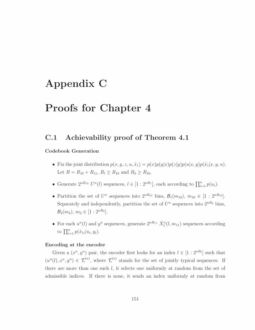
Appendix C
Proofs for Chapter 4
C.1 Achievability proof of Theorem 4.1
Codebook Generation
• Fix the joint distribution p(x, y, z, u, x1) = p(x)p(y|x)p(z|y)p(u|x, y)p(x1|x, y, u).
Let R = R10 +R11, Rl ≥ R10 and R2 ≥ R10.
• Generate 2nR10 Un(l) sequences, l ∈ [1 : 2nR1 ], each according to∏n
i=1 p(ui).
• Partition the set of Un sequences into 2nR10 bins, B1(m10), m10 ∈ [1 : 2nR10 ].
Separately and independently, partition the set of Un sequences into 2nR2 bins,
B2(m2), m2 ∈ [1 : 2nR2].
• For each un(l) and yn sequences, generate 2nR11 Xn1 (l, m11) sequences according
to∏n
i=1 p(x1i|ui, yi).
Encoding at the encoder
Given a (xn, yn) pair, the encoder first looks for an index l ∈ [1 : 2nRl] such that
(un(l), xn, yn) ∈ T (n)ǫ , where T (n)
ǫ stands for the set of jointly typical sequences. If
there are more than one such l, it selects one uniformly at random from the set of
admissible indices. If there is none, it sends an index uniformly at random from
151
[1 : 2nRl]1. Next, it finds the index m11 such that (x1(l, m11), un(m10), x
n, yn) ∈ T(n)ǫ .
As before, if there is more than one, it selects one uniformly at random from the set
of admissible indices. If there is none, it sends an index uniformly at random from
[1 : 2nR11 ]. Finally, it sends out (m10, m11), where m10 is the bin index such that
un(l) ∈ B1(m10). The total rate required is R.
Decoding and reconstruction at Node 1
Given (m10, m11), Node 1 looks for the unique l such that (un(l), yn) ∈ T(n)ǫ and
un(l) ∈ B1(l). It reconstructs xn as xn(l, m11). If it failed to find a unique one, or if
there is more than one, it outputs l = 1 and performs the reconstruction as before.
Encoding at Node 1
Node 1 sends an index m2 such that un(l) ∈ B2(m2). This requires a rate of R2.
Decoding and reconstruction at Node 2
Node 2 looks for the index l such that (un(l), yn) ∈ T(n)ǫ and l ∈ B2(m2). It then
reconstructs xn according to x2i = g2(un(l)i, zi) for i ∈ [1 : n]. If there is no such
index, it reconstructs using l = 1.
Analysis of expected distortion
Using the typical average lemma in [13, Lecture 2] and following the analysis
in [13, Lecture 3], it suffices to analyze the probability of “error”; i.e. the probability
that the chosen sequences will not be jointly typical with the source sequences. Let L
and M11 be the chosen indices at the encoder. Note that these define the bin indices
M10 and M2. Let M2 be the chosen index at Node 1. Define the following error
events:
1. E0 := {(Xn, Y n) /∈ T(n)ǫ }
2. E1 := {(Un(l), Xn, Y n) /∈ T(n)ǫ } for all l ∈ [1 : 2nRl]
3. E2 := {(Un(l), Xn, Y n, Zn) /∈ T(n)ǫ } for all l ∈ [1 : 2nRl]
4. E3 := {(Un(L), Xn(L,m11), Xn, Y n) /∈ T
(n)ǫ } for all m11 ∈ [1 : 2nR11]
1For simplicity, we assume randomized encoding, but it is easy to see that the randomizedencoding employed our proofs can be incorporated as part of the (random) codebook generationstage.
152

APPENDIX C. PROOFS FOR CHAPTER 4 153
5. E4 := {(Un(l), Y n) ∈ T(n)ǫ } for some l 6= L and Un(l) ∈ B1(M10)
6. E5(M2) := {(Un(l), Zn) ∈ T(n)ǫ } for some l 6= L and Un(l) ∈ B2(M2)
We can then bound the probability of error as
Pe ≤ P{5⋃
i=0
Ei} =∑
P{Ei ∩ (i−1⋂
j=0
E cj )}.
• P{E0} → 0 as n → ∞ by Law of Large Numbers (LLN).
• By the covering lemma in [13, Lecture 3], P{E1 ∩ E c0} → 0 as n → ∞ if
Rl > I(U ;X, Y ) + δ(ǫ).
• P{E2 ∩E c1 ∩E c
0} → 0 as n → ∞ by the Markov relation U − (X, Y )−Z and the
conditional joint typicality lemma [13, Lecture 2].
• By the covering lemma in [13, Lecture 3], P{E3 ∩ (⋂2
j=0 Ecj} → 0 as n → ∞ if
R11 > I(X1;X|U, Y ) + δ(ǫ).
• From the analysis of the Wyner-Ziv Coding scheme (see [36] or [13, Lecture
12]), P{E4 ∩ (⋂3
j=0 Ecj} → 0 as n → ∞ if
Rl −R10 < I(U ; Y )− δ(ǫ).
• For the last term, we have
P{E5(M2) ∩ (4⋂
j=0
E cj )}=P{E5(M2) ∩ (
4⋂
j=0
E cj ) ∩ {M2 6= M2}}
+ P{E5(M2) ∩ (
4⋂
j=0
E cj ) ∩ {M2 = M2}}
(a)= P{E5(M2) ∩ (
4⋂
j=0
E cj ) ∩ {M2 = M2}}
= P{E5(M2) ∩ (
4⋂
j=0
E cj ) ∩ {M2 = M2}}
≤ P{E5(M2) ∩ E c2}.
Step (a) follows from the observation that (⋂4
j=0 Ecj ) ∩ {M2 6= M2} = ∅. The
analysis of the probability of error therefore reduces to the analysis for the
equivalent Wyner-Ziv setup with Z as the side information at Node 2. Hence,
P{E5(M2) ∩ (⋂4
j=0 Ecj )} → 0 as n → ∞ if
Rl −R2 < I(U ;Z)− δ(ǫ).
Eliminating Rl in the aforementioned inequalities then gives us the required rate re-
gion.
C.2 Achievability proof of Theorem 4.2
As the achievability proof for the Triangular Source Coding Case follows that of
the Cascade Source Coding Case closely, we will only include the additional steps
required for generating R3 and analysis of probability of error at Node 2. The steps
for generating R1 and R2, and for reconstruction at Node 1 are the same as the
Cascade setup.
Codebook Generation
• Fix p(x, y, z, u, v, x1) = p(x)p(y|x)p(z|y)p(u|x, y)p(x1|x, y, u)p(v|x, y, u).
• For each un(l), generate V n(l3), l3 ∈ [1 : 2nR3], according to∏n
i=1 p(vi|ui).
Partition the set of vn sequences into 2nR3 bins, B3(m3).
Encoding
154

APPENDIX C. PROOFS FOR CHAPTER 4 155
• Given a sequence (xn, yn) and un(l) found through the steps in the Cascade
Source Coding setup, the encoder looks for an index l3 such that (un, vn(l, l3), xn, yn) ∈
T(n)ǫ . If it finds more than one, it selects one uniformly at random from the set
of admissible indices. If it finds none, it outputs an index uniformly at random
from [1 : 2nR3 ]. The encoder then sends out m3 such that L3 ∈ B3(m3).
Decoding
The additional decoding step is in decoding L3. Node 2 looks for the unique l3
such that (un(l), vn(l, l3), zn) ∈ T
(n)ǫ and vn(l3) ∈ B3(M3). If there is none or more
than one, it outputs m3 = 1.
Analysis of Distortion
Let L, M11 and M3 be the indices chosen by the encoder. Note that these fix the
indices M10 and M2. We follow similar analysis as in the Cascade case, with the same
definitions for error events E0 to E5. We also require the following additional error
events:
7) E6 := {(Un(L), V n(L, L3), Xn, Y n) /∈ T
(n)ǫ }.
8) E7 := {(Un(L), V n(L, L3), Xn, Y n, Zn) /∈ T
(n)ǫ }.
9) E8(L) := {(Un(L), V n(L, l3), Zn) ∈ T
(n)ǫ } for some l3 6= L3 and l3 ∈ B3(M3).
To bound the probability of error, we have the following additional terms
• By the covering lemma, P(E6 ∩ E c2) → 0 as n → ∞ if
R3 > I(V ;X, Y |U) + δ(ǫ).
• P(E7 ∩ E c6) → 0 as n∞ from the Markov condition (V, U)− (X, Y )−Z and the
conditional joint typicality lemma.
• P{E8(L) ∩ E c5(M2) ∩ E c
7 ∩ (⋂4
j=0 Ecj ))}. We have
P{E8(L) ∩ E c5(M2) ∩ E c
7 ∩ (
4⋂
j=0
E cj )}

= P{E8(L) ∩ E c5(M2) ∩ E c
7 ∩ (4⋂
j=0
E cj ) ∩ {M2 = M2}}
+ P{E8(L) ∩ E c5(M2) ∩ E c
7 ∩ (
4⋂
j=0
E cj ) ∩ {M2 6= M2}}
= P{E8(L) ∩ E c5(M2) ∩ E c
7 ∩ (
4⋂
j=0
E cj ) ∩ {M2 = M2}}
= P
{
E8(L) ∩ E c5(M2) ∩ E c
7 ∩ (4⋂
j=0
E cj ) ∩ {M2 = M2}
}
≤ P{E8(L) ∩ E c5(M2) ∩ E c
7}
(a)= P{E8(L) ∩ E c
5(M2) ∩ E c7 ∩ {L = L}}
= P{E8(L) ∩ E c5(M2) ∩ E c
7 ∩ {L = L}}
≤ P{E8(L) ∩ E c7}.
(a) follows from the observation that E c5(M2) ∩ E c
7 ∩ {L 6= L} = ∅. It remains
to bound P{E8(L) ∩ E c7}. Note that the analysis of this term is equivalent to
analyzing the setup where Un is the side information at Node 0 and (Un, Zn) is
the side information at Node 2. Hence, P{E8(L) ∩ E c7} → 0 as n → ∞ if
R3 − R3 < I(V ;Z|U)− δ(ǫ).
We then obtain the rate region by eliminating R3 and Rl.
C.3 Achievability proof of Theorem 4.3
As with the case for the Triangular setting, the proof for this case follows the Cascade
setting closely. We will therefore include only the additional steps. We have a change
of notation from the Cascade setting. We will use U1 instead of U .
Codebook Generation
156
APPENDIX C. PROOFS FOR CHAPTER 4 157
• Fix p(x, y, z, u1, u2, x1) = p(x, y, z)p(u1|x, y)p(x1|u1, x, y)p(u2|z, u1).
• For each un1(l), generate 2nR3 Un
2 (l3) sequences, l ∈ [1 : 2nR3], each according to∏n
i=1 p(u2i|u1i). Partition the set of Un2 into 2nR3 bins, B3(m3).
Encoding
The additional encoding step is at Node 2. Node 2 looks for an index L3 such that
(un1(L), u
n2 (L, L3), Z
n) ∈ T(n)ǫ . As before, if it finds more than one, it selects an index
uniformly at random from the set of admissible indices. If it finds none, it outputs
an index uniformly at random from [1 : 2nR3 ]. It then outputs the bin index m3 such
that L3 ∈ B3(m3).
Decoding
Additional decoding is required at Node 0. Node 0 looks the index l3 such that
(un1(l), u
n2(l, l3), x
n, yn) ∈ T(n)ǫ and l3 ∈ B3(m3).
Analysis of distortion
Let ECascade denote the event that an error occurs in the forward Cascade path.
In addition, we define the following error events.
• ETW−1(L) := {(Un1 (L), U
n2 (L, l3), Z
n) /∈ T(n)ǫ for all l3 ∈ [1 : 2nR3 ]}.
• ETW−2(L) := {(Un1 (L), U
n2 (L, L3), Z
n, Xn, Y n) /∈ T (n)ǫ }.
• ETW−3(L) := {(Un1 (L), U
n2 (L, l3), X
n, Y n) ∈ T(n)ǫ for some l3 ∈ B3(M3), l3 6=
L3}.
• P(ETW−1(L) ∩ E cCascade) = P(ETW−1(L) ∩ E c
Cascade) → 0 as n → ∞ if
R3 > I(U2;Z|U1) + δ(ǫ).
• P(ETW−2(L) ∩ E cCascade) = P(ETW−2(L) ∩ E c
Cascade) → 0 as n → ∞ by the strong
Markov Lemma [32].
• P(ETW−3(L) ∩ E cCascade) = P(ETW−3(L) ∩ E c
Cascade) → 0 as n → ∞ if
R3 − R3 < I(U2;X, Y |U1)− δ(ǫ).

Finally, eliminating R3 and Rl gives us the required rate region.
C.4 Achievability proof of Theorem 4.4
The achievability proof for Two Way Triangular source coding combines the proofs
of the Triangular source coding case and the Two-way cascade case. As it is largely
similar to these proofs, we will not repeat it here. We will just mention that the
codebook generation, encoding, decoding and analysis of distortion for the forward
path from Node 0 to Node 2 follows that of the Triangular source coding case, while
codebook generation, encoding, decoding and analysis of distortion for the reverse
path from Node 2 to Node 0 follows that of the Two-way Cascade source coding case,
with (U2, V ) taking the role of U2.
C.5 Cardinality Bounds
We provide cardinality bounds for Theorems 4.1-4.4 stated in Chapter 4. The main
tool we will use is the Fenchel-Eggleston-Caratheodory Theorem [9].
Proof of cardinality bound for Theorem 4.1
For each x, y, we have
fj(pX,Y |U(x, y|u)) =∑
u
p(u)p(x, y|u) = p(x, y).
We therefore have |X ||Y|−1 continuous functions of p(x, y|u). These set of equations
preserves the distribution p(x, y) and hence, by Markovity, p(x, y, z). Next, observe
that the following are similarly continuous functions of p(x, y|u)
I(U ;X, Y |Z) = H(X, Y |Z)−H(X, Y, Z|U) +H(Z|U),
I(X ; X1, U |Y ) = H(X|Y )−H(X|U) +H(X, X1, Y |U),
E d1(X, X1) =∑
x,x
p(x, x1)d(x, x1),
158
APPENDIX C. PROOFS FOR CHAPTER 4 159
E d2(X, X2) =∑
x,y,u
p(x, y, u)d(x, g2(x, u)),
These equations give us 4 additional continuous functions and hence, by Fenchel-
Eggleston-Caratheodory Theorem, there exists a U ′ with cardinality of |X ||Y|+3 such
that all the constraints are satisfied. Note that this construction does not preserve
p(x1), but this does not change the rate-distortion region since the associated rate
and distortion are preserved.
Proof of cardinality bound for Theorem 4.2
We will first give a bound for the cardinality of U . We look at the following
continuous functions of p(x, y|u).
fj(pX,Y |U(x, y|u)) =∑
u
p(u)p(x, y|u) = p(x, y), ∀x, y
I(U ;X, Y |Z) = H(X, Y |Z)−H(X, Y, Z|U) +H(Z|U),
I(X ; X1, U |Y ) = H(X|Y )−H(X|U) +H(X, X1, Y |U),
I(X, Y ;V |U,Z) = H(X, Y, Z|U)−H(Z|U)−H(X, Y, V, Z|U) +H(V, Z|U),
E d1(X, X1) =∑
x,x
p(x, x1)d(x, x1),
E d2(X, X2) =∑
x,y,u,v
p(x, y, u, v)d(x, g2(x, u)).
From these equations, there exists a U ′ with |U ′| ≤ |X ||Y|+4 such that the equations
are satisfied. Note that the new U ′ induces a new V ′. For each U ′ = u, consider the
following continuous functions of p(x, y|u, v)
p(x, y|u) =∑
v
p(v|u)p(x, y|v, u),
I(X, Y ;V |U = u, Z) = H(X, Y |U = u, Z)−H(X, Y |V, U = u, Z),
E(d2(X, X2)|U = u) =∑
x,y,v
p(x, y, v|u)d(x, g2(x, u)).
From this set of equations, we see that for each U ′ = u, it suffices to consider V ′
such that |V ′| ≤ |X ||Y| + 1. Hence, the overall cardinality bound on V is |V| ≤

(|X ||Y|+ 4)(|X ||Y|+ 1). The joint p(x, y, z) is preserved due to the Markov Chain
(V, U)− (X, Y )− Z.
Proof of cardinality bound for Theorem 4.3
The cardinality bounds on U1 follows similar analysis as in the Cascade source
coding case. The proof is therefore omitted. For each U1 = u1, the following are
continuous functions of p(z|u2, u1),
p(z|u1) =∑
u2
p(u2|u1)p(z|u2, u1),
I(U2;Z|U1 = u1, X, Y ) = H(Z|U1 = u1, X, Y )−H(Z|U1 = u1, U2, X, Y ),
E(d3(Z, Z)|U1 = u1) =∑
x,y,z,u2
(p(x, y, z, u2|u1)d(z, g3(x, y, u1, u2))) .
From this set of equations, we see that for each U1 = u1, it suffices to consider U ′2 such
that |U ′2| ≤ |Z|+1. Hence, the overall cardinality bound on U2 is |U2| ≤ |U1|(|Z|+1).
The joint p(x, y, z) is preserved due to the Markov Chains U1 − (X, Y ) − Z and
U2 − (Z, U1)− (X, Y ).
Proof of cardinality bound for Theorem 4.4
The cardinality bounds follow similar steps to those for the first 3 theorems. For
the cardinality bound for |U2|, we find a cardinality bound for each U1 = u1 and
V = v. Details of the proof are omitted.
C.6 Alternative characterizations of rate distor-
tion regions in Corollaries 4.1 and 4.2
In this appendix, we show that the rate distortion regions in Corollaries 4.1 and 4.2
can alternatively be characterized by transforming them into equivalent problems
found in [27], where explicit characterizations were given. We focus on the Cascade
case (Corollary 4.1), since the Triangular case follows by the same analysis.
Figure C.1 shows the Cascade source coding setting which the optimization prob-
lem in Corollary 4.1 solves.
160
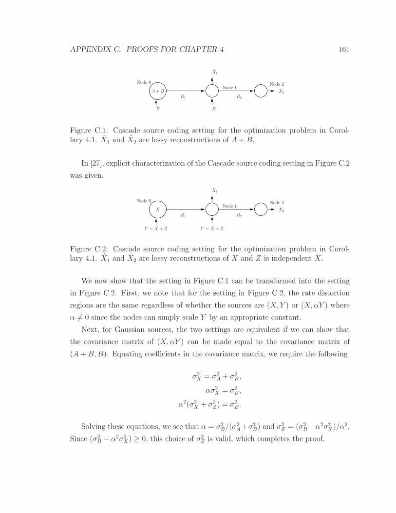
APPENDIX C. PROOFS FOR CHAPTER 4 161
A +B
BB
R1 R2
X1
X2
Node 0Node 1
Node 2
Figure C.1: Cascade source coding setting for the optimization problem in Corol-lary 4.1. X1 and X2 are lossy reconstructions of A+B.
In [27], explicit characterization of the Cascade source coding setting in Figure C.2
was given.
X
Y = X + ZY = X + Z
R1 R2
X1
X2
Node 0Node 1
Node 2
Figure C.2: Cascade source coding setting for the optimization problem in Corol-lary 4.1. X1 and X2 are lossy reconstructions of X and Z is independent X .
We now show that the setting in Figure C.1 can be transformed into the setting
in Figure C.2. First, we note that for the setting in Figure C.2, the rate distortion
regions are the same regardless of whether the sources are (X, Y ) or (X,αY ) where
α 6= 0 since the nodes can simply scale Y by an appropriate constant.
Next, for Gaussian sources, the two settings are equivalent if we can show that
the covariance matrix of (X,αY ) can be made equal to the covariance matrix of
(A+B,B). Equating coefficients in the covariance matrix, we require the following
σ2X = σ2
A + σ2B,
ασ2X = σ2
B,
α2(σ2X + σ2
Z) = σ2B.
Solving these equations, we see that α = σ2B/(σ
2A+σ2
B) and σ2Z = (σ2
B−α2σ2X)/α
2.
Since (σ2B − α2σ2
X) ≥ 0, this choice of σ2Z is valid, which completes the proof.
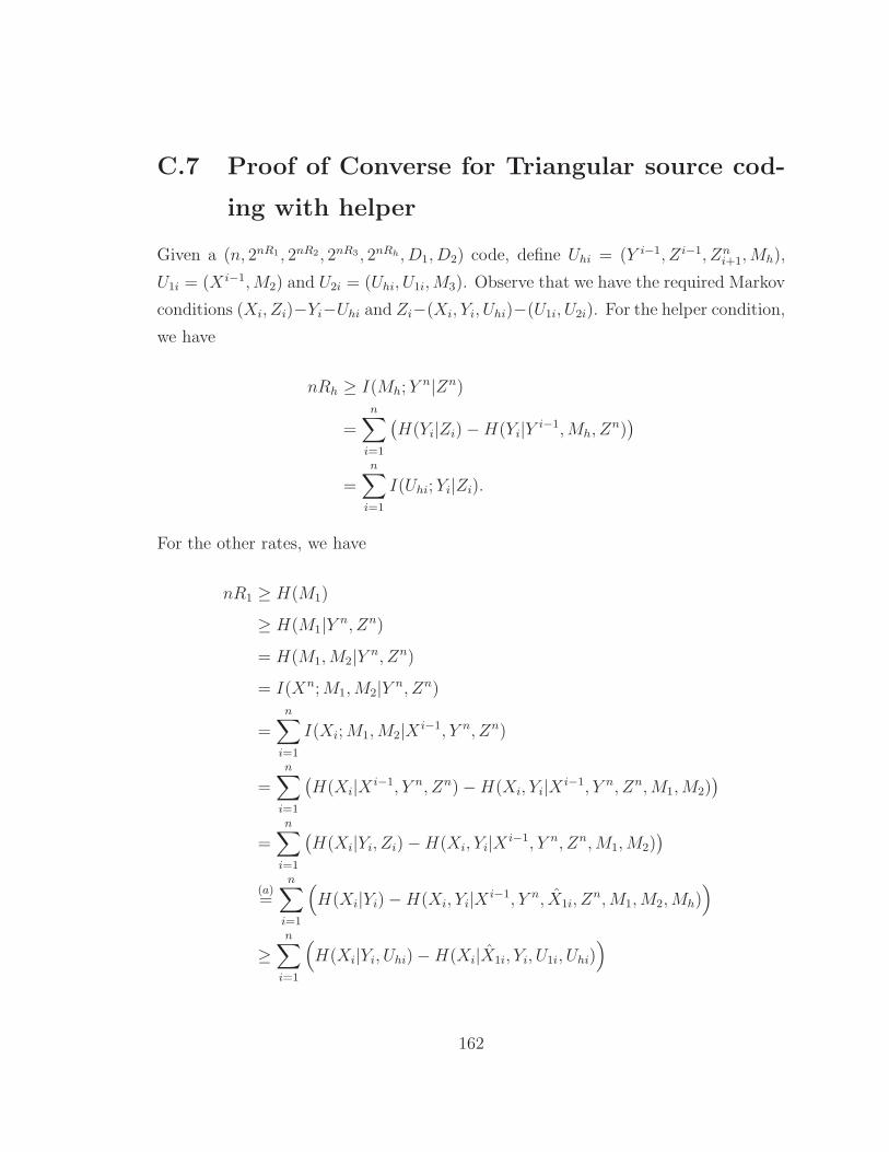
C.7 Proof of Converse for Triangular source cod-
ing with helper
Given a (n, 2nR1, 2nR2, 2nR3 , 2nRh, D1, D2) code, define Uhi = (Y i−1, Z i−1, Zni+1,Mh),
U1i = (X i−1,M2) and U2i = (Uhi, U1i,M3). Observe that we have the required Markov
conditions (Xi, Zi)−Yi−Uhi and Zi−(Xi, Yi, Uhi)−(U1i, U2i). For the helper condition,
we have
nRh ≥ I(Mh; Yn|Zn)
=
n∑
i=1
(
H(Yi|Zi)−H(Yi|Yi−1,Mh, Z
n))
=
n∑
i=1
I(Uhi; Yi|Zi).
For the other rates, we have
nR1 ≥ H(M1)
≥ H(M1|Yn, Zn)
= H(M1,M2|Yn, Zn)
= I(Xn;M1,M2|Yn, Zn)
=n∑
i=1
I(Xi;M1,M2|Xi−1, Y n, Zn)
=
n∑
i=1
(
H(Xi|Xi−1, Y n, Zn)−H(Xi, Yi|X
i−1, Y n, Zn,M1,M2))
=n∑
i=1
(
H(Xi|Yi, Zi)−H(Xi, Yi|Xi−1, Y n, Zn,M1,M2)
)
(a)=
n∑
i=1
(
H(Xi|Yi)−H(Xi, Yi|Xi−1, Y n, X1i, Z
n,M1,M2,Mh))
≥n∑
i=1
(
H(Xi|Yi, Uhi)−H(Xi|X1i, Yi, U1i, Uhi))
162
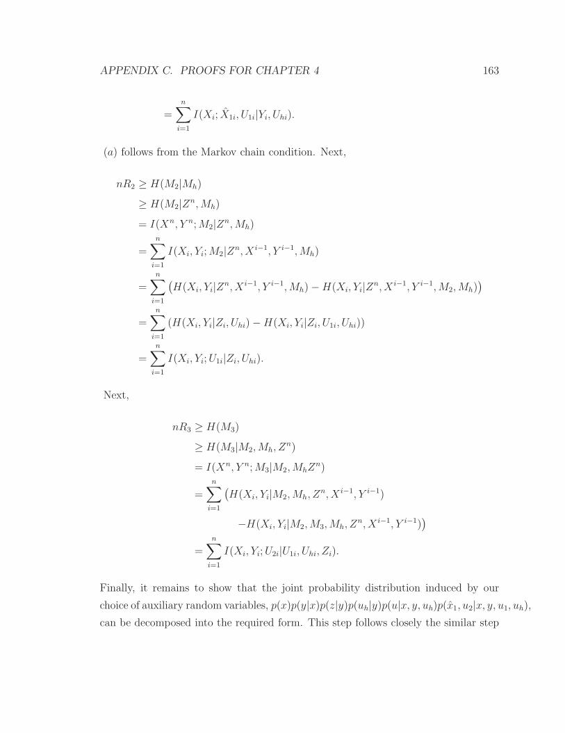
APPENDIX C. PROOFS FOR CHAPTER 4 163
=n∑
i=1
I(Xi; X1i, U1i|Yi, Uhi).
(a) follows from the Markov chain condition. Next,
nR2 ≥ H(M2|Mh)
≥ H(M2|Zn,Mh)
= I(Xn, Y n;M2|Zn,Mh)
=
n∑
i=1
I(Xi, Yi;M2|Zn, X i−1, Y i−1,Mh)
=
n∑
i=1
(
H(Xi, Yi|Zn, X i−1, Y i−1,Mh)−H(Xi, Yi|Z
n, X i−1, Y i−1,M2,Mh))
=n∑
i=1
(H(Xi, Yi|Zi, Uhi)−H(Xi, Yi|Zi, U1i, Uhi))
=
n∑
i=1
I(Xi, Yi;U1i|Zi, Uhi).
Next,
nR3 ≥ H(M3)
≥ H(M3|M2,Mh, Zn)
= I(Xn, Y n;M3|M2,MhZn)
=
n∑
i=1
(
H(Xi, Yi|M2,Mh, Zn, X i−1, Y i−1)
−H(Xi, Yi|M2,M3,Mh, Zn, X i−1, Y i−1)
)
=n∑
i=1
I(Xi, Yi;U2i|U1i, Uhi, Zi).
Finally, it remains to show that the joint probability distribution induced by our
choice of auxiliary random variables, p(x)p(y|x)p(z|y)p(uh|y)p(u|x, y, uh)p(x1, u2|x, y, u1, uh),
can be decomposed into the required form. This step follows closely the similar step

in the proof of Theorem 4.2, which we therefore omit.
164

Bibliography
[1] Rudolph Ahlswede and Imre Csiszar. Common randomness in information theory
and cryptography—I: Secret sharing. IEEE Trans. Inf. Theory, 39(4), 1993.
[2] Ehsan Ardestanizadeh, Massimo Franceschetti, Tara Javidi, and Young Han
Kim. Wiretap channel with rate-limited feedback. IEEE Trans. Inf. Theory,
55(12):5353–5361, December 2009.
[3] G. Bagherikaram, A. S. Motahari, and A. K. Khandani. The secrecy rate region of
the broadcast channel. In 46th Annual Allerton Conference on Communication,
Control and Computing, Sept 2008.
[4] S. Borade, L. Zheng, and M. Trott. Multilevel broadcast networks. In Interna-
tional Symposium on Information Theory, 2007.
[5] Yanling Chen and A. J. Han Vinck. Wiretap channel with side information.
IEEE Trans. Inf. Theory, 54(1):395–402, 2006.
[6] T. Cover and J. Thomas. Elements of Information Theory 2nd edition. Wiley
Interscience, July 2006.
[7] I. Csiszar and J. Korner. Broadcast channels with confidential messages. IEEE
Trans. Inf. Theory, IT-24:339–348, May 1978.
[8] Paul Cuff, Han-I Su, and Abbas El Gamal. Cascade multiterminal source cod-
ing. In ISIT’09: Proceedings of the 2009 IEEE international conference on Sym-
posium on Information Theory, pages 1199–1203, Piscataway, NJ, USA, 2009.
IEEE Press.
165
[9] H. G. Eggleston. Convexity. Cambridge: Cambridge University Press, 1958.
[10] E. Ekrem and S. Ulukus. Secrecy capacity of a class of broadcast channels with an
eavesdropper. EURASIP Journal on Wireless Communications and Networking,
Oct 2009.
[11] Abbas El Gamal. The feedback capacity of degraded broadcast channels (cor-
resp.). IEEE Transactions on Information Theory, 24(3):379–381, May 1978.
[12] Abbas El Gamal. The capacity of a class of broadcast channels. IEEE Trans.
Info. Theory, 25(2):166–169, Mar 1979.
[13] Abbas El Gamal and Young Han Kim. Network Information Theory. Cambridge
University Press, 1st edition, 2011.
[14] Abbas El Gamal and E. C. van der Meulen. A proof of marton’s coding theorem
for the discrete memoryless broadcast channel. IEEE Transactions on Informa-
tion Theory, 27(1):120–121, 1981.
[15] W. H. Gu and M. Effros. Source coding for a simple multi-hop network. In IEEE
International Symposium on Information Theory, ISIT, pages 2335–2339, June
28- July 3 2005.
[16] P. Ishwar and S. S. Pradhan. A relay-assisted distributed source coding problem,.
In ITA Workshop, 2008.
[17] Amiram H. Kaspi. Two-way source coding with a fidelity criterion. IEEE Trans.
Inf. Theory, 31(6):735–740, 1985.
[18] A. Khisti, A. Tchamkerten, and G.W. Wornell. Secure broadcasting over fading
channels. IEEE Trans. Info. Theory, 54(6):2453–2469, June 2008.
[19] Ashish Khisti, Suhas N. Diggavi, and Gregory W. Wornell. Secret key agree-
ment using asymmetry in channel state knowledge. In Proc. IEEE International
Symposium on Information Theory, pages 2286–2290, Seoul, South Korea, July
2009.
166
BIBLIOGRAPHY 167
[20] J. Korner and K. Marton. Comparison of two noisy channels. In Topics in
Information Theory (Second Colloq., Keszthely, 1975), pages 411–423, 1977.
[21] Yingbin Liang, H. V. Poor, and Shlomo Shamai. Information theoretic secu-
rity. Foundations and Trends in Communications and Information Theory, 5(4–
5):355–580, 2008.
[22] Ruoheng Liu, I. Maric, P. Spasojevic, and R. D. Yates. Discrete memoryless
interference and broadcast channels with confidential messages: Secrecy rate
regions. IEEE Trans. Info. Theory, 54(6):2493–2507, June 2008.
[23] Wei Liu and Biao Chen. Wiretap channel with two-sided state information. In
Proc. 41st Asilomar Conf. Signals, Systems and Comp., pages 893–897, Pacific
Grove, CA, November 2007.
[24] Katalin Marton. A coding theorem for the discrete memoryless broadcast chan-
nel. IEEE Trans. Info. Theory, 25(3):306–311, May 1979.
[25] Ueli M. Maurer. Secret key agreement by public discussion from common infor-
mation. IEEE Trans. Inf. Theory, 39(3):733–742, 1993.
[26] Chandra Nair and Abbas El Gamal. The capacity region of a class of 3-receiver
broadcast channels with degraded message sets. IEEE Trans. Info. Theory, 2008.
Submitted. Available online at http://arxiv.org/abs/0712.3327.
[27] Haim Permuter and Tsachy Weissman. Cascade and triangular source coding
with side information at the first two nodes. Online at ArXiv: arXiv:1001.1679v.
[28] Claude E. Shannon. Communication theory of secrecy systems. Bell Systems
Tech. J., 28:656–715, 1949.
[29] Claude E. Shannon. Channels with side information at the transmitter. IBM J.
Res. Develop., 2:289–293, 1958.
[30] Yossef Steinberg and Neri Merhav. On successive refinement for the wyner-ziv
problem, ccit rep. 419, ee pub. 1358. Technical report, Technion Department of
Electrical Engineering, 2003.
[31] R. Timo and B.N. Vellambi. Two lossy source coding problems with causal side-
information. In IEEE International Symposium on Information Theory, ISIT,
pages 1040–1044, June 28- July 3 2009.
[32] S.-Y. Tung. Multiterminal source coding. PhD thesis, Cornell University, Itahca,
NY, 1978.
[33] D. Vasudevan, C. Tian, and S. N. Diggavi. Lossy source coding for a cascade
communication system with side informations. In Proceeding of Allerton confer-
ence on Communication, Control and Computing, 2006.
[34] Tsachy Weissman and Abbas El Gamal. Source coding with limited-look-ahead
side information at the decoder. IEEE Trans. Inf. Theory, 52(12):5218–5239,
2006.
[35] F. M. J. Willems and E. C. van der Meulen. The discrete memoryless multiple-
access channel with cribbing encoders. IEEE Trans. Inf. Theory, 31(3):313–327,
1985.
[36] A. D. Wyner. The wire-tap channel. Bell System Technical Journal, 54(8):1355–
1387, 1975.
[37] A. D.Wyner. The rate-distortion function for source coding with side information
at the decoder-ii: General sources. Information and Control, (38:60-80), 1978.
[38] A. D. Wyner and J. Ziv. The rate-distortion function for source coding with side
information at the decoder. IEEE Trans. Inf. Theor., 22(1):1–10, 1976.
[39] H. Yamamoto. Source coding theory for cascade and branching communication
systems. IEEE Trans. Inf. Theory, 27:299–308, 1981.
[40] Hirosuke Yamamoto. Rate-distortion theory for the Shannon cipher system.
IEEE Trans. Inf. Theory, 43(3):827–835, 1997.
168