Abstract of “A Multi-Scale Model of Brain White-Matter Structure and Its Fitting Method for Dif-

fusion MRI” by Jadrian Miles, Ph.D., Brown University, May 2015.

This dissertation describes three primary contributions to the field of medical imaging: (1) a math-

ematical model (“Blockhead”) of the macroscopic and microscopic structure of the white matter of

the human brain; (2) a technique for computing the parameters of such a model from MRI scans

of a given subject; and (3) an application of existing statistical tools to compare instances of any

different tissue models according to their accuracy and parsimony with respect to MR images of the

subject. The Blockhead model has both discrete and continuous parameters. As such the fitting

method demonstrates a novel synthesis of techniques from combinatorial and numerical optimiza-

tion: namely, the inclusion of short gradient-descent steps into the neighborhood of a local-search

solver. The thesis of this work is that this multi-scale tissue model admits of an instance that, for

certain inputs with simple geometry, has better fit to the input (in the sense of accuracy and parsi-

mony) than current voxel-oriented techniques. Furthermore the fitting method is capable, in some

circumstances, of computing this model instance. The dissertation also details the shortcomings of

this model and proposes future refinements to better represent realistic tissue geometry.

A Multi-Scale Model of Brain White-Matter Structure and Its Fitting Method for Diffusion MRI

by

Jadrian Miles

B. S., Duke University, 2006

Sc. M., Brown University, 2008

A dissertation submitted in partial fulfillment of the

requirements for the Degree of Doctor of Philosophy

in the Department of Computer Science at Brown University

Providence, Rhode Island

May 2015

© Copyright 2015 by Jadrian Miles

This dissertation by Jadrian Miles is accepted in its present form by

the Department of Computer Science as satisfying the dissertation requirement

for the degree of Doctor of Philosophy.

DateDavid H. Laidlaw, Director

Recommended to the Graduate Council

DateJohn F. Hughes, Reader

DateBen Raphael, Reader

DatePeter J. Basser, Reader

NIH

Approved by the Graduate Council

DatePeter Weber

Dean of the Graduate School

iii

Acknowledgements

This dissertation is dedicated in memory of my grandfather, Jere Myers. I continue to aspire to his

kindness, patience, enthusiasm, and giving spirit.

It is also dedicated to Providence, Rhode Island, my home for seven years during my graduate

studies. Providence had a transformative influence on my life; I can’t imagine another place that

could have shaped, inspired, and nurtured me as much as this city did.

I am grateful for the support and guidance of countless people in my journey to, through, and out

the other side of graduate school. My advisor, David Laidlaw, has been a friend and mentor since

I met him, and I deeply appreciate his advice and prodding throughout my work, as well as his

purposeful forbearance as I chose my own directions in research and life. I thank my dissertation

committee: Spike Hughes, Ben Raphael, and particularly Peter Basser, whose active involvement,

encouragement, and feedback greatly improved my work. Thanks also to Erik Sudderth for helpful

feedback on statistical methods; and to the Brown CS astaff and tstaff for their help over many

years, particularly Lauren Clarke, Dawn Reed, and Genie deGouveia. I thank my early professors

Dan Teague and Robert Duvall, who opened my eyes to the academic path I’ve traveled. I thank

my Providence communities, in particular the graduate students of Brown across disciplines, my

colleagues and students at New Urban Arts, and every artist and musician whose work touched my

life at Building 16, AS220, Pronk, RISD, Brown, 186 Carpenter, and so on. I should refrain from

naming all of the mentors, family, and friends who have supported and encouraged me through this

endeavor (among so many others), but here’s a sampling: Jonathan, Ken, Linda, Elsie, Adj, Nick,

Suzy, Andreas, Ryan, Sean, Erin, Frank, Pippin, and David G. I hope I can pass on what you’ve

given to me.

v

vi

Contents

1 Introduction and Background 1

1.1 Overview . . . . . . . . . . . . . . . . . . . . . . . . . . . . . . . . . . . . . . . . . . 1

1.1.1 Terminology . . . . . . . . . . . . . . . . . . . . . . . . . . . . . . . . . . . . 4

1.2 Brain Structure . . . . . . . . . . . . . . . . . . . . . . . . . . . . . . . . . . . . . . . 5

1.3 Diffusion MRI . . . . . . . . . . . . . . . . . . . . . . . . . . . . . . . . . . . . . . . . 6

1.4 Microstructure Modeling . . . . . . . . . . . . . . . . . . . . . . . . . . . . . . . . . . 9

1.4.1 Incorporating More Data into Microstructure Fitting . . . . . . . . . . . . . . 11

1.5 Macrostructure Modeling . . . . . . . . . . . . . . . . . . . . . . . . . . . . . . . . . 12

1.6 Noise Properties of Diffusion MRI . . . . . . . . . . . . . . . . . . . . . . . . . . . . 13

1.6.1 Estimating the Noise Level of MR Images . . . . . . . . . . . . . . . . . . . . 15

1.7 Comparison of Diffusion Models . . . . . . . . . . . . . . . . . . . . . . . . . . . . . . 15

1.7.1 Rician Log-Likelihood . . . . . . . . . . . . . . . . . . . . . . . . . . . . . . . 16

1.7.2 Foreground Masking . . . . . . . . . . . . . . . . . . . . . . . . . . . . . . . . 16

2 The “Blockhead” Model of White-Matter Structure 19

2.1 Introduction . . . . . . . . . . . . . . . . . . . . . . . . . . . . . . . . . . . . . . . . . 19

2.2 Methods . . . . . . . . . . . . . . . . . . . . . . . . . . . . . . . . . . . . . . . . . . . 19

2.2.1 Model . . . . . . . . . . . . . . . . . . . . . . . . . . . . . . . . . . . . . . . . 19

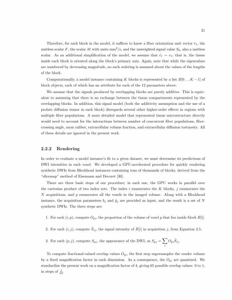
2.2.2 Rendering . . . . . . . . . . . . . . . . . . . . . . . . . . . . . . . . . . . . . . 21

2.2.3 Computing the AIC . . . . . . . . . . . . . . . . . . . . . . . . . . . . . . . . 22

2.2.4 Numerical Optimization . . . . . . . . . . . . . . . . . . . . . . . . . . . . . . 22

2.3 Evaluation . . . . . . . . . . . . . . . . . . . . . . . . . . . . . . . . . . . . . . . . . . 26

2.3.1 Model-Instance Comparison . . . . . . . . . . . . . . . . . . . . . . . . . . . . 27

2.4 Results and Discussion . . . . . . . . . . . . . . . . . . . . . . . . . . . . . . . . . . . 28

2.4.1 DT vs. CSD . . . . . . . . . . . . . . . . . . . . . . . . . . . . . . . . . . . . 28

2.4.2 DT vs. Blockhead Oracle . . . . . . . . . . . . . . . . . . . . . . . . . . . . . 31

2.4.3 DT vs. Gradient-Descent Blockhead Fit . . . . . . . . . . . . . . . . . . . . . 31

2.5 Conclusions . . . . . . . . . . . . . . . . . . . . . . . . . . . . . . . . . . . . . . . . . 35

3 Discrete–Continuous Optimization 37

3.1 Introduction . . . . . . . . . . . . . . . . . . . . . . . . . . . . . . . . . . . . . . . . . 37

3.2 Methods . . . . . . . . . . . . . . . . . . . . . . . . . . . . . . . . . . . . . . . . . . . 37

vii

3.2.1 Local Search Moves . . . . . . . . . . . . . . . . . . . . . . . . . . . . . . . . 37

3.2.2 Search Metaheuristics . . . . . . . . . . . . . . . . . . . . . . . . . . . . . . . 39

3.2.3 Initialization . . . . . . . . . . . . . . . . . . . . . . . . . . . . . . . . . . . . 41

3.2.4 Termination . . . . . . . . . . . . . . . . . . . . . . . . . . . . . . . . . . . . . 41

3.3 Evaluation . . . . . . . . . . . . . . . . . . . . . . . . . . . . . . . . . . . . . . . . . . 41

3.4 Results and Discussion . . . . . . . . . . . . . . . . . . . . . . . . . . . . . . . . . . . 42

3.4.1 Wrong Numbers of Blocks . . . . . . . . . . . . . . . . . . . . . . . . . . . . . 44

3.4.2 Incorrect Fiber Orientation . . . . . . . . . . . . . . . . . . . . . . . . . . . . 44

3.4.3 Curved Geometry . . . . . . . . . . . . . . . . . . . . . . . . . . . . . . . . . 46

3.5 Conclusions . . . . . . . . . . . . . . . . . . . . . . . . . . . . . . . . . . . . . . . . . 50

4 Physical-Phantom Experiments 51

4.1 Introduction . . . . . . . . . . . . . . . . . . . . . . . . . . . . . . . . . . . . . . . . . 51

4.2 Methods and Evaluation . . . . . . . . . . . . . . . . . . . . . . . . . . . . . . . . . . 51

4.3 Results and Discussion . . . . . . . . . . . . . . . . . . . . . . . . . . . . . . . . . . . 53

4.4 Conclusions . . . . . . . . . . . . . . . . . . . . . . . . . . . . . . . . . . . . . . . . . 55

5 Conclusions and Open Problems 57

5.1 Optimization . . . . . . . . . . . . . . . . . . . . . . . . . . . . . . . . . . . . . . . . 57

5.2 Tissue Modeling . . . . . . . . . . . . . . . . . . . . . . . . . . . . . . . . . . . . . . 57

5.3 Open Questions . . . . . . . . . . . . . . . . . . . . . . . . . . . . . . . . . . . . . . . 58

Bibliography 61

viii

List of Figures

1.1 Illustrations from Gray’s Anatomy of some major white-matter fascicles . . . . . . . 2

1.2 An axial block-face photograph of the brain, and a cartoon of a neuron . . . . . . . 5

1.3 Two diffusion-weighted MR images of the same brain . . . . . . . . . . . . . . . . . . 7

1.4 Stejskal–Tanner diffusion signal as a function of b . . . . . . . . . . . . . . . . . . . . 8

1.5 Visualizations of common models of anisotropic diffusion . . . . . . . . . . . . . . . . 9

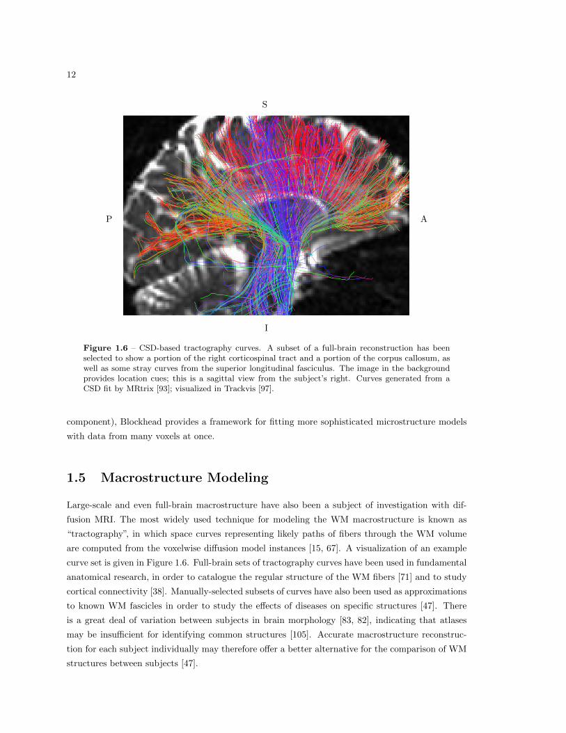
1.6 CSD-based tractography curves . . . . . . . . . . . . . . . . . . . . . . . . . . . . . . 12

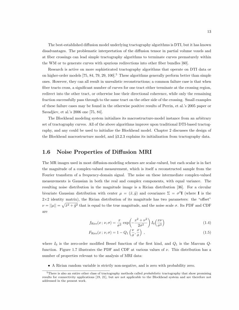
1.7 The PDF and CDF of the Rician distribution . . . . . . . . . . . . . . . . . . . . . . 14

2.1 The eight computational phantoms . . . . . . . . . . . . . . . . . . . . . . . . . . . . 24

2.2 Initial Blockhead instances for gradient descent . . . . . . . . . . . . . . . . . . . . . 25

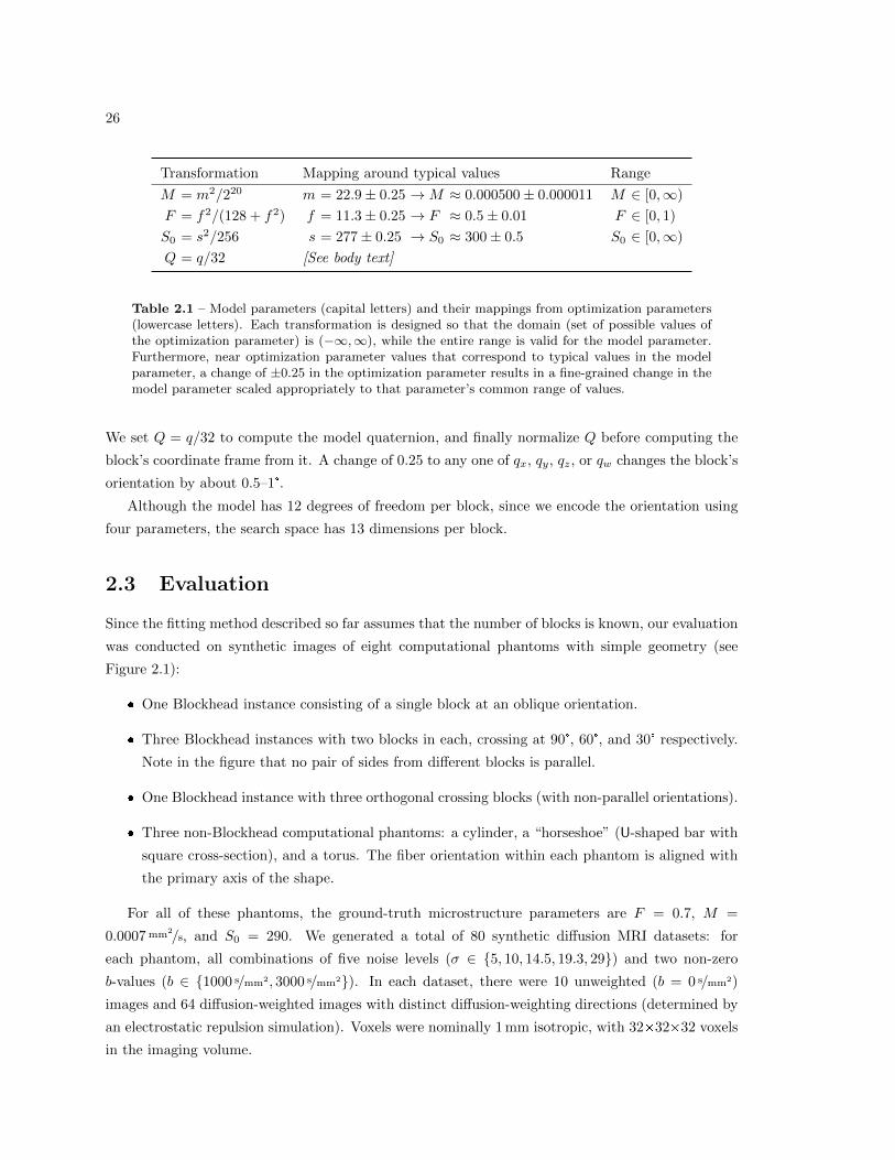
2.3 Model-fit comparison for voxelwise models . . . . . . . . . . . . . . . . . . . . . . . . 29

2.4 Model-fit comparison for DT and Blockhead oracles . . . . . . . . . . . . . . . . . . 30

2.5 −log(L) image for Blockhead oracle of a crossing-fiber subject . . . . . . . . . . . . . 31

2.6 Blockhead gradient-descent fits for several challenging subjects . . . . . . . . . . . . 32

2.7 Model-fit comparison for DT and Blockhead gradient-descent fit . . . . . . . . . . . 33

3.1 Model-fit comparison for DT and Blockhead discrete–continuous fit . . . . . . . . . . 43

3.2 Blockhead discrete–continuous fits with the wrong number of blocks . . . . . . . . . 45

3.3 Blockhead discrete–continuous fits with incorrect fiber orientation . . . . . . . . . . 47

3.4 Unsuccessful fits on curved-geometry phantoms . . . . . . . . . . . . . . . . . . . . . 48

3.5 Successful fits on curved-geometry phantoms . . . . . . . . . . . . . . . . . . . . . . 49

4.1 DWIs of the Fiber Cup phantom . . . . . . . . . . . . . . . . . . . . . . . . . . . . . 52

4.2 Initial Blockhead model instance . . . . . . . . . . . . . . . . . . . . . . . . . . . . . 53

4.3 Blockhead discrete–continuous fits for Fiber Cup datasets . . . . . . . . . . . . . . . 54

5.1 A whole specimen of the occipitofrontal fasciculus . . . . . . . . . . . . . . . . . . . 59

ix

List of Tables

2.1 Model parameters and their mappings from optimization parameters . . . . . . . . . 26

2.2 SNR at various noise levels . . . . . . . . . . . . . . . . . . . . . . . . . . . . . . . . 27

2.3 Basic measures of the experimental subjects . . . . . . . . . . . . . . . . . . . . . . . 28

2.4 Model-fit comparison on the singleton subject . . . . . . . . . . . . . . . . . . . . . . 33

3.1 Summary of discrete–continuous optimization experiments . . . . . . . . . . . . . . . 42

4.1 Basic measures of the Fiber Cup phantom images . . . . . . . . . . . . . . . . . . . . 52

x

List of Algorithms

3.1 Selecting a random local-search move . . . . . . . . . . . . . . . . . . . . . . . . . . . 40

xi

xii

Chapter 1

Introduction and Background

This dissertation describes “Blockhead”, a novel system for modeling human brain-tissue structure,

which comprises a mathematical model and its associated fitting method. The input to this system

is a set of images gathered from a brain scan of a particular modality, namely diffusion MRI. Brain

tissue has structural features both above and below the resolution of the input images, leading to a

challenging modeling problem with both discrete and continuous properties. Blockhead models the

tissue at both scales, and uses local search to iteratively adjust all model parameters. This chapter

reviews material related to brain anatomy, diffusion MRI, and statistics, as well as related work in

tissue modeling.

1.1 Overview

Blockhead focuses on modeling brain tissue, in particular the white matter. The other primary type

of neural tissue, the grey matter, does the majority of the cognitive processing, is located on the

surface of the brain and in certain interior structures, and has historically been the primary subject

of neuroscience investigation. The white matter, on the other hand, is located entirely in the interior,

and is relatively less well-studied. (White matter and grey matter are also found elsewhere in nervous

system, but here we focus only on the brain.) The white matter is made up of billions of long, thin

axons: projections of neurons, each about a micron in diameter and up to several centimeters long.

These axons act as biological wires, connecting different regions of grey matter to each other and

to the body. Axons that originate near each other in one location, and terminate near each other

somewhere else, tend to follow the same path through the brain. In this way, higher-level structures

called “tracts” arise that consist of hundreds of thousands of aligned axons. Similar tracts group

together into “fascicles”, which may be millimeters in diameter and therefore visible to the naked

eye. Anatomists have known of many fascicles in the brain for more than a century (see Figure 1.1).

Before the mid-1990s, however, the only ways to study the anatomical structure of the white matter

were dissection and histology. In the case of human brains, of course, these are ex-vivo techniques:

they require the subject to be deceased.

More recently, a non-invasive imaging technique called “diffusion-weighted magnetic resonance

imaging”, or “diffusion MRI”, has enabled the indirect, in-vivo observation of white-matter structure.

Diffusion MRI measures, at a chosen location and in a chosen direction, bulk properties of the random

1

2

(a) Gray’s 718 — A coronal section of the brain showing white and grey matter.

(b) Gray’s 751 — A sagittal section of the brain showing major white-matter fascicles.

Figure 1.1 – Plates from the 1918 edition of Gray’s Anatomy [35].

3

motion of water molecules. Since the fibrous structure of the white matter affects the motion of water

molecules differently in different directions, diffusion MRI is sensitive to the local orientation and

composition of white-matter fibers. In 1994, Basser, et al. [14] described diffusion tensor imaging, the

first and still most widely used model for interpreting diffusion MRI data and correlating it to white-

matter structure. Since then, many efforts have been made to improve techniques for interpreting

diffusion MRI data in terms of white-matter structure; this dissertation is one such effort.

The output of a diffusion MRI scan is a set of so-called “diffusion-weighted images” (DWIs),

which are the principal inputs to the algorithms described herein. Each DWI is a raster volume—

that is, a regular three-dimensional grid of voxels, the volumetric analogue of pixels; see Figure 1.3

for two example images. Each voxel in a DWI corresponds to a small volume (usually a cube

approximately 2 mm on a side) in the space inside the MRI scanner. Models of white-matter structure

derived from diffusion MRI therefore generally separate into two regimes: “macrostructure” models

that explicitly describe structures larger than a voxel, and “microstructure” models that describe

statistical summaries (such as the mean or a simple distribution) of the structural properties of

populations of axons in volumes about the size of a voxel. In this context, the macrostructure of

the white matter is the shape, orientation, and position of tracts and fascicles. The microstructure

of the white matter includes all the structural properties of individual axons—their trajectories,

diameters, spacing, permeability, etc.—described in aggregate.

While most previous approaches in this field have focused on only one or the other of these

regimes, the Blockhead model combines macrostructure and microstructure into a single represen-

tation. In this model, each discrete macrostructure element (defined by a surface representation of

its boundary) also stores a statistical description of the microstructure properties throughout its

volume that affect its image in the sensor.

The Blockhead fitting method is a local-search optimization over a virtual space of candidate

model instances. The fundamental requirement of local search is the ability to evaluate an objective

function for a given model instance. The objective function used in the present work is the Akaike

information criterion, a statistical measure that balances model parsimony against accuracy of pre-

dictions. The values to be predicted in this case are MRI signals: a perfectly accurate model would

predict exactly the signal values that make up the input images. The Blockhead fitter uses a novel

GPU-accelerated renderer to compute a “synthetic image” of the diffusion MRI signals predicted by

a given model instance.

The chapters of this dissertation build on each other as follows:

� The remainder of Chapter 1 provides background and context for this work: the mechanism

and noise properties of diffusion MRI, biological observations and modeling considerations for

white-matter microstructure and macrostructure, and statistical tools for evaluating tissue

model instances.

� Chapter 2 describes the Blockhead model of white-matter macrostructure and microstruc-

ture, a numerical optimization method for its parameters under some strong assumptions, and

experiments that demonstrate the feasibility of the fitting and evaluation methods.

4

� Chapter 3 relaxes the assumptions from the previous chapter and presents a hybrid discrete–

continuous optimization method for the Blockhead model, followed by further experiments.

� Chapter 4 applies the discrete–continuous optimization method to fitting the Blockhead model

to a physical phantom.

� Chapter 5 includes closing remarks regarding the advantages and limitations of the Blockhead

model, as well as proposals for future refinements and discussion of open problems.

1.1.1 Terminology

Throughout this document, certain terms will be used with specific intended meanings. These may

not correspond to the meanings understood in other documents within the brain-modeling literature

or in other fields of study or contexts. However, they are used consistently within this text, and the

meanings described here apply only within this text.

“Macrostructure” denotes white-matter fiber trajectories at the millimeter scale as well as the

morphology of the gross segments of brain tissue: coherent white-matter structures and contiguous

volumes of grey matter or cerebrospinal fluid. “WM”, “GM”, and “CSF” respectively refer to these

tissue and fluid types. The scope of this work is restricted to the brain, and therefore WM and GM

refer specifically to the white matter and grey matter of the brain; the spinal cord also contains these

tissues, but is excluded from this work. The terms “axon”, “fiber”, “tract”, and “fascicle” refer to

the levels of the anatomical hierarchy of the white matter of a real brain, in order of increasing size.

“Microstructure” denotes the characteristics of the white matter on a sub-millimeter level, including

details of fluid exchange, fluid self-diffusion, and cell geometry. “Model” denotes a mathematical

model—a set of parameters and a consistent interpretation thereof—while an “instance” of that

model is a particular set of values assigned to the parameters.

A “phantom” is a synthetic structure used as a subject for imaging or image analysis; phan-

toms enable a broad array of experiments because they provide known ground truth. A “physical

phantom” is an actual object that is placed in the scanner and imaged, whereas a “computational

phantom” is a geometrical model instance used to generate synthetic images.

When describing location and orientation in the brain, special terminology is used. “Posterior”

and “anterior” mean “back” and “front”, respectively; “inferior” and “superior” mean “bottom” and

“top”; and, in this work, “left” and “right” are from the subject’s perspective. These terms may

also be used as adjectives to describe relative position: “anterior”, for example, may mean “toward

the front”. The three orientations of axis-aligned planes also have special names. A “sagittal” plane

divides the left-right axis and is parallel to the other two axes; the “mid-sagittal” plane divides the

face, head, and brain into symmetrical halves. A “coronal” plane divides the posterior-anterior axis;

a coronal plane through the ears, for example, would divide the face from the back of the head.

An “axial”, “transverse”, or “horizontal” plane divides the inferior-superior axis; when the subject

is standing and looking straight ahead, an axial plane is parallel to the ground.

5

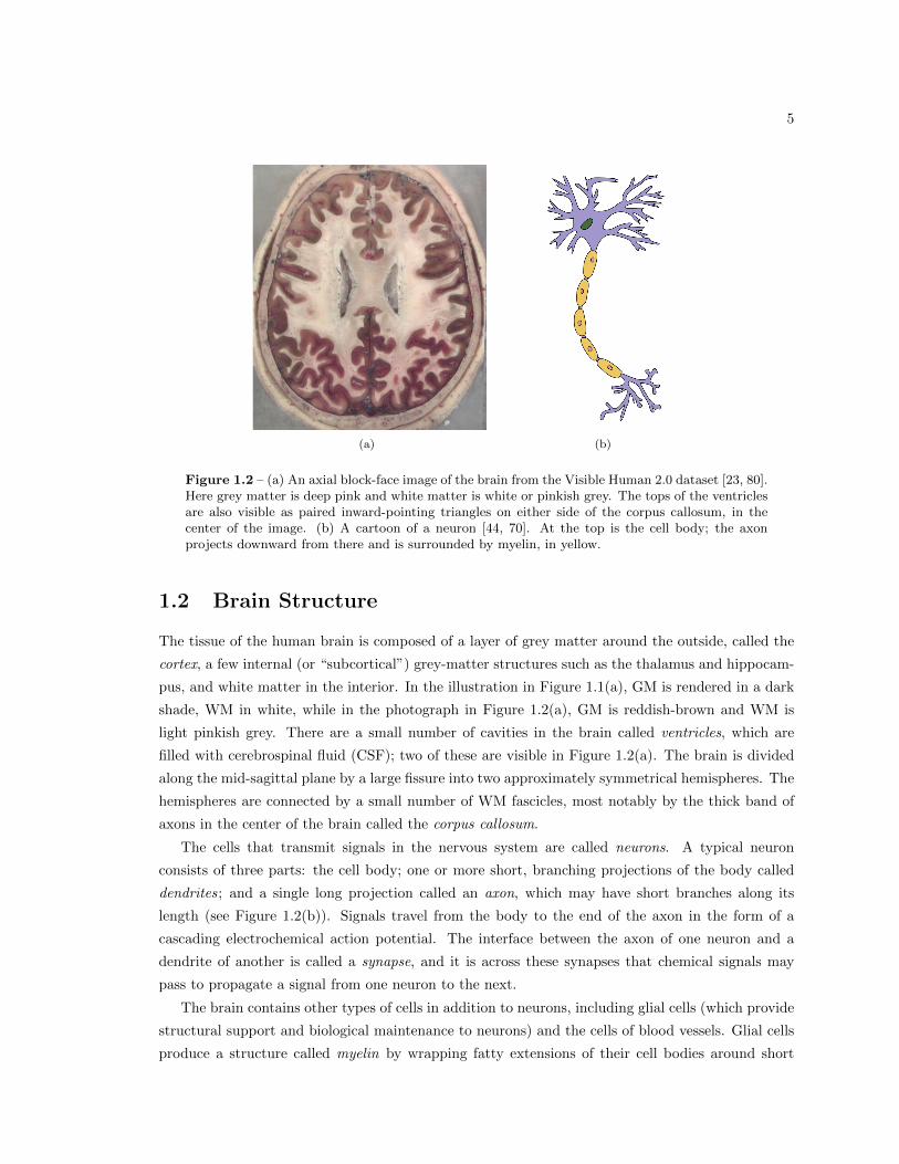
(a) (b)

Figure 1.2 – (a) An axial block-face image of the brain from the Visible Human 2.0 dataset [23, 80].Here grey matter is deep pink and white matter is white or pinkish grey. The tops of the ventriclesare also visible as paired inward-pointing triangles on either side of the corpus callosum, in thecenter of the image. (b) A cartoon of a neuron [44, 70]. At the top is the cell body; the axonprojects downward from there and is surrounded by myelin, in yellow.

1.2 Brain Structure

The tissue of the human brain is composed of a layer of grey matter around the outside, called the

cortex, a few internal (or “subcortical”) grey-matter structures such as the thalamus and hippocam-

pus, and white matter in the interior. In the illustration in Figure 1.1(a), GM is rendered in a dark

shade, WM in white, while in the photograph in Figure 1.2(a), GM is reddish-brown and WM is

light pinkish grey. There are a small number of cavities in the brain called ventricles, which are

filled with cerebrospinal fluid (CSF); two of these are visible in Figure 1.2(a). The brain is divided

along the mid-sagittal plane by a large fissure into two approximately symmetrical hemispheres. The

hemispheres are connected by a small number of WM fascicles, most notably by the thick band of

axons in the center of the brain called the corpus callosum.

The cells that transmit signals in the nervous system are called neurons. A typical neuron

consists of three parts: the cell body; one or more short, branching projections of the body called

dendrites; and a single long projection called an axon, which may have short branches along its

length (see Figure 1.2(b)). Signals travel from the body to the end of the axon in the form of a

cascading electrochemical action potential. The interface between the axon of one neuron and a

dendrite of another is called a synapse, and it is across these synapses that chemical signals may

pass to propagate a signal from one neuron to the next.

The brain contains other types of cells in addition to neurons, including glial cells (which provide

structural support and biological maintenance to neurons) and the cells of blood vessels. Glial cells

produce a structure called myelin by wrapping fatty extensions of their cell bodies around short

6

segments of certain axons. A so-called “myelinated” axon is wrapped in myelin along its entire

length (except for small gaps between adjacent myelin segments), forming a myelin sheath that

increases the propagation rate of the nerve signals along that axon.

Each axon in the WM of the brain is a projection of a neuronal body in one location and

terminates in another location, typically several centimeters away. The body of a neuron that

transmits signals from a grey-matter site is located close to the interface between the white matter

and the grey matter at that site. The distal (far) end of an axon that transmits signals to a grey-

matter site is similarly located close to the WM/GM boundary at that site. Thus, apart from glial

cells, blood vessels, and other cells, the white matter is primarily composed of axons.

If two neuronal bodies near each other have axons that terminate near each other, the axons tend

to stay near each other along their lengths, and hence white-matter fibers arise from great numbers

of locally parallel axons that connect different sites together. Individual axons in the human brain

white matter typically range from 0.5µm to 20µm in diameter [6], while fiber diameters are on the

millimeter scale.

In a given white-matter fiber, axonal membranes and myelin sheaths are oriented approximately

parallel to each other. Within each axon, the nanoscale fibers of the neuron’s cytoskeleton are also

aligned parallel to the axon itself. All these structures hinder or restrict the random motion of water

molecules both inside and outside the cells, making water diffuse faster along the fiber axis than

across it. Diffusion MRI analysis exploits this orientational dependence (or “anisotropy”) to detect

structural properties of the white matter [18].

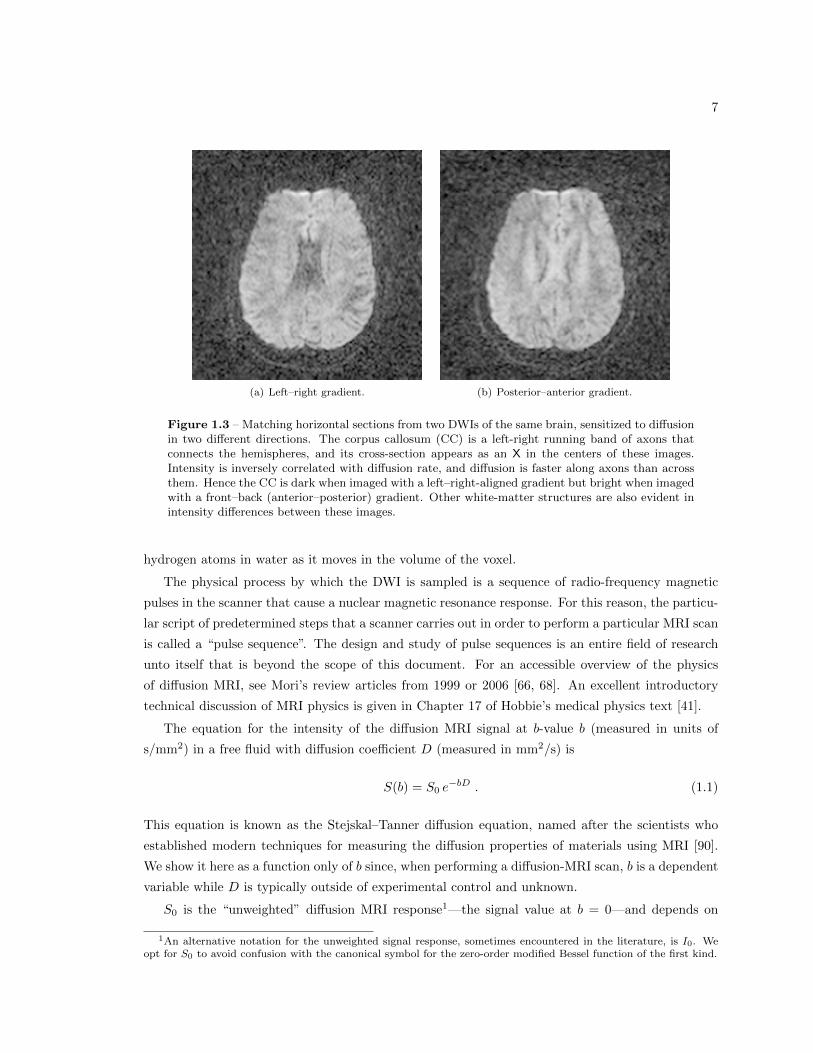
1.3 Diffusion MRI

Each diffusion-weighted image (DWI) that results from a diffusion MRI scan measures water self-

diffusion in a chosen direction and over a chosen time scale. “Self-diffusion” of water molecules

specifically means their diffusion in the absence of a chemical gradient, or simply the diffusion of

water molecules in an environment of water, with no net flux. The value in a particular voxel in this

DWI is a noisy measurement related to the average diffusion (in this direction and over this time

scale) of all water molecules in the volume of the voxel. Each DWI has two imaging parameters

associated with it: a b-value, which is related to the time scale, and a diffusion gradient vector, which

dictates the direction. Each DWI in a diffusion MRI acquisition may have a different b-value and

gradient vector. Some example DWIs are given in Figure 1.3. For reasons explained below, there are

almost always at least 7 DWIs in an acquisition, often as many as 70, and sometimes many more.

Let us consider an example acquisition with n DWIs, and a small volume the size of a voxel

surrounding a single point in the interior of the brain. This volume has n diffusion measurements

associated with it: one for the corresponding voxel in each DWI. Therefore a properly co-registered

set of DWIs may be conceived of as a single raster volume whose value in each voxel is a length-n

vector, rather than as n separate scalar-valued raster volumes. Each of the n components of the

vector in each voxel is a physical measurement of a magnetic resonance response from the nuclei of

7

(a) Left–right gradient. (b) Posterior–anterior gradient.

Figure 1.3 – Matching horizontal sections from two DWIs of the same brain, sensitized to diffusionin two different directions. The corpus callosum (CC) is a left-right running band of axons thatconnects the hemispheres, and its cross-section appears as an X in the centers of these images.Intensity is inversely correlated with diffusion rate, and diffusion is faster along axons than acrossthem. Hence the CC is dark when imaged with a left–right-aligned gradient but bright when imagedwith a front–back (anterior–posterior) gradient. Other white-matter structures are also evident inintensity differences between these images.

hydrogen atoms in water as it moves in the volume of the voxel.

The physical process by which the DWI is sampled is a sequence of radio-frequency magnetic

pulses in the scanner that cause a nuclear magnetic resonance response. For this reason, the particu-

lar script of predetermined steps that a scanner carries out in order to perform a particular MRI scan

is called a “pulse sequence”. The design and study of pulse sequences is an entire field of research

unto itself that is beyond the scope of this document. For an accessible overview of the physics

of diffusion MRI, see Mori’s review articles from 1999 or 2006 [66, 68]. An excellent introductory

technical discussion of MRI physics is given in Chapter 17 of Hobbie’s medical physics text [41].

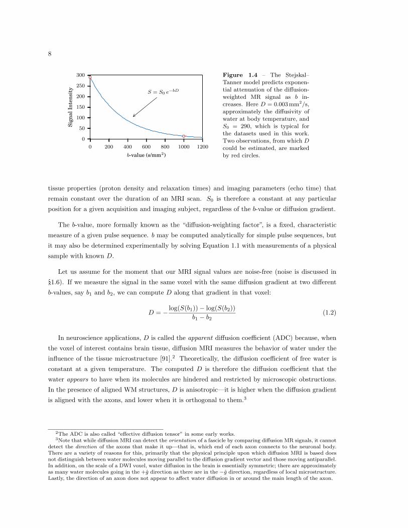
The equation for the intensity of the diffusion MRI signal at b-value b (measured in units of

s/mm2) in a free fluid with diffusion coefficient D (measured in mm2/s) is

S(b) = S0 e−bD . (1.1)

This equation is known as the Stejskal–Tanner diffusion equation, named after the scientists who

established modern techniques for measuring the diffusion properties of materials using MRI [90].

We show it here as a function only of b since, when performing a diffusion-MRI scan, b is a dependent

variable while D is typically outside of experimental control and unknown.

S0 is the “unweighted” diffusion MRI response1—the signal value at b = 0—and depends on

1An alternative notation for the unweighted signal response, sometimes encountered in the literature, is I0. Weopt for S0 to avoid confusion with the canonical symbol for the zero-order modified Bessel function of the first kind.

8

0 200 400 600 800 1000 1200

b-value (s/mm2)

0

50

100

150

200

250

300Si

gnal

Inte

nsit

y

S = S0 e−bD

Figure 1.4 – The Stejskal–Tanner model predicts exponen-tial attenuation of the diffusion-weighted MR signal as b in-creases. Here D = 0.003 mm2/s,approximately the diffusivity ofwater at body temperature, andS0 = 290, which is typical forthe datasets used in this work.Two observations, from which Dcould be estimated, are markedby red circles.

tissue properties (proton density and relaxation times) and imaging parameters (echo time) that

remain constant over the duration of an MRI scan. S0 is therefore a constant at any particular

position for a given acquisition and imaging subject, regardless of the b-value or diffusion gradient.

The b-value, more formally known as the “diffusion-weighting factor”, is a fixed, characteristic

measure of a given pulse sequence. b may be computed analytically for simple pulse sequences, but

it may also be determined experimentally by solving Equation 1.1 with measurements of a physical

sample with known D.

Let us assume for the moment that our MRI signal values are noise-free (noise is discussed in

§1.6). If we measure the signal in the same voxel with the same diffusion gradient at two different

b-values, say b1 and b2, we can compute D along that gradient in that voxel:

D = − log(S(b1))− log(S(b2))

b1 − b2(1.2)

In neuroscience applications, D is called the apparent diffusion coefficient (ADC) because, when

the voxel of interest contains brain tissue, diffusion MRI measures the behavior of water under the

influence of the tissue microstructure [91].2 Theoretically, the diffusion coefficient of free water is

constant at a given temperature. The computed D is therefore the diffusion coefficient that the

water appears to have when its molecules are hindered and restricted by microscopic obstructions.

In the presence of aligned WM structures, D is anisotropic—it is higher when the diffusion gradient

is aligned with the axons, and lower when it is orthogonal to them.3

2The ADC is also called “effective diffusion tensor” in some early works.3Note that while diffusion MRI can detect the orientation of a fascicle by comparing diffusion MR signals, it cannot

detect the direction of the axons that make it up—that is, which end of each axon connects to the neuronal body.There are a variety of reasons for this, primarily that the physical principle upon which diffusion MRI is based doesnot distinguish between water molecules moving parallel to the diffusion gradient vector and those moving antiparallel.In addition, on the scale of a DWI voxel, water diffusion in the brain is essentially symmetric; there are approximatelyas many water molecules going in the +g direction as there are in the −g direction, regardless of local microstructure.Lastly, the direction of an axon does not appear to affect water diffusion in or around the main length of the axon.

9

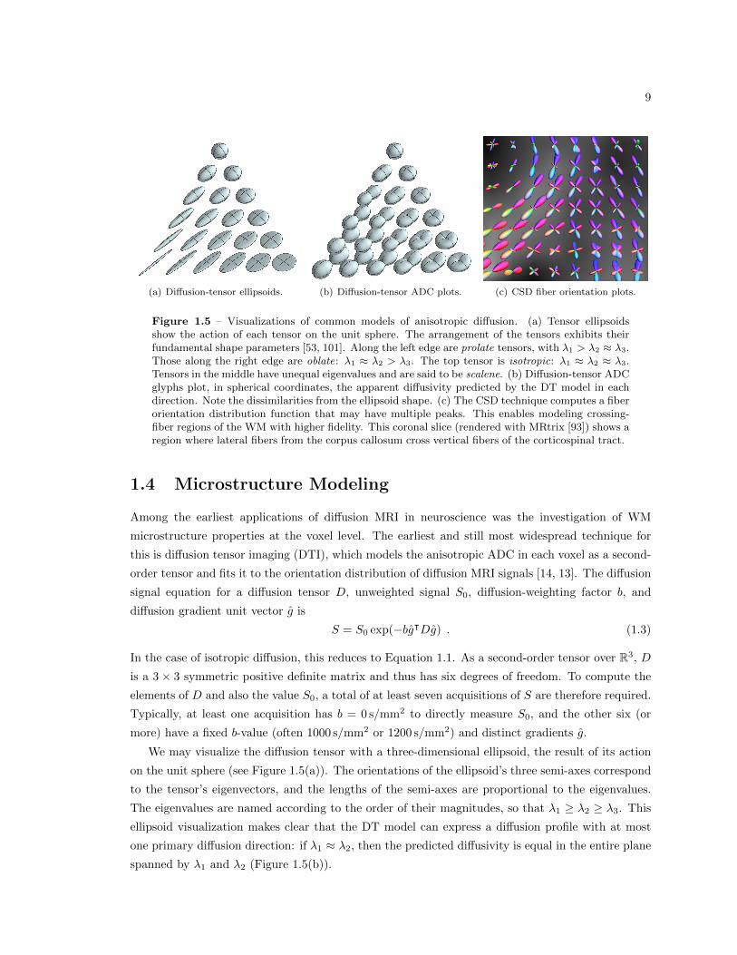
(a) Diffusion-tensor ellipsoids. (b) Diffusion-tensor ADC plots. (c) CSD fiber orientation plots.

Figure 1.5 – Visualizations of common models of anisotropic diffusion. (a) Tensor ellipsoidsshow the action of each tensor on the unit sphere. The arrangement of the tensors exhibits theirfundamental shape parameters [53, 101]. Along the left edge are prolate tensors, with λ1 > λ2 ≈ λ3.Those along the right edge are oblate: λ1 ≈ λ2 > λ3. The top tensor is isotropic: λ1 ≈ λ2 ≈ λ3.Tensors in the middle have unequal eigenvalues and are said to be scalene. (b) Diffusion-tensor ADCglyphs plot, in spherical coordinates, the apparent diffusivity predicted by the DT model in eachdirection. Note the dissimilarities from the ellipsoid shape. (c) The CSD technique computes a fiberorientation distribution function that may have multiple peaks. This enables modeling crossing-fiber regions of the WM with higher fidelity. This coronal slice (rendered with MRtrix [93]) shows aregion where lateral fibers from the corpus callosum cross vertical fibers of the corticospinal tract.

1.4 Microstructure Modeling

Among the earliest applications of diffusion MRI in neuroscience was the investigation of WM

microstructure properties at the voxel level. The earliest and still most widespread technique for

this is diffusion tensor imaging (DTI), which models the anisotropic ADC in each voxel as a second-

order tensor and fits it to the orientation distribution of diffusion MRI signals [14, 13]. The diffusion

signal equation for a diffusion tensor D, unweighted signal S0, diffusion-weighting factor b, and

diffusion gradient unit vector g is

S = S0 exp(−bgᵀDg) . (1.3)

In the case of isotropic diffusion, this reduces to Equation 1.1. As a second-order tensor over R3, D

is a 3 × 3 symmetric positive definite matrix and thus has six degrees of freedom. To compute the

elements of D and also the value S0, a total of at least seven acquisitions of S are therefore required.

Typically, at least one acquisition has b = 0 s/mm2 to directly measure S0, and the other six (or

more) have a fixed b-value (often 1000 s/mm2 or 1200 s/mm2) and distinct gradients g.

We may visualize the diffusion tensor with a three-dimensional ellipsoid, the result of its action

on the unit sphere (see Figure 1.5(a)). The orientations of the ellipsoid’s three semi-axes correspond

to the tensor’s eigenvectors, and the lengths of the semi-axes are proportional to the eigenvalues.

The eigenvalues are named according to the order of their magnitudes, so that λ1 ≥ λ2 ≥ λ3. This

ellipsoid visualization makes clear that the DT model can express a diffusion profile with at most

one primary diffusion direction: if λ1 ≈ λ2, then the predicted diffusivity is equal in the entire plane

spanned by λ1 and λ2 (Figure 1.5(b)).

10

Though the diffusion tensor model does not directly represent the microstructure, the orienta-

tion of its principal eigenvector is correlated with the local axon orientation, and other structural

properties affect the tensor as well [68]. To quantify these effects, researchers developed a variety of

measures of the diffusion tensor, including the popular tensor invariant called “fractional anisotropy”

(FA) [16]. Especially in clinically-oriented research, voxelwise analysis with DTI, and particularly

FA, continues to be the most common use of the technology [55, 62, 52, 34].

However, the diffusion tensor model has widely acknowledged disadvantages. In partial-volume

voxels (where crossing fibers, or distinct fiber populations or tissue types, coexist in the same voxel),

a single tensor cannot express the diffusion characteristics of the multiple tissue populations. Even

in single-population voxels, the tensor fit is sensitive to image resolution and other acquisition

parameters [3, 76, 96, 4]. FA and other anisotropy measures also suffer from ambiguous interpretation

in terms of actual tissue properties. Demyelination, axon dropout, and mixed fiber populations, for

example, can all cause a decrease in anisotropy [68].

Numerous researchers have developed alternative techniques for interpreting diffusion signals in

each voxel, in an attempt to overcome the shortcomings of the diffusion-tensor model. Some fit

multiple tensors [20, 42, 74], while others compute higher-order representations or decompositions of

the diffusion profile, from which useful measures may be derived [5, 32, 96, 40, 99]. One such model,

which we use as a baseline for comparison throughout this dissertation, is constrained spherical

deconvolution (CSD) [94, 92, 95]. CSD estimates an orientation distribution function for the fibers

in each voxel and represents it in a spherical harmonic basis. This fiber orientation distribution

(FOD) may have multiple peaks, representing distinct crossing fiber populations (see Figure 1.5(c)).

CSD computes the FOD by first estimating, from the DWIs, the signal profile of a single-fiber

population in a known orientation. It then deconvolves the observed signals in each voxel by the

single-fiber profile to arrive at the FOD. Although the assumption that all fiber populations have the

same signal profile does not accurately reflect reality, CSD is a successful technique for distinguishing

crossing fiber populations and produces good results when used as input for higher-level modeling

of macrostructure (see Figure 1.6).

Another class of appealing approaches are the so-called compartment models. These models

directly represent the microstructural properties of the tissue in each sample. Parameters include

orientation of the axon population, diffusion coefficients of the intra- and extracellular fluid, volume

fractions of the various fluid compartments, axon diameter or “caliber” (or a distribution thereof),

and fluid exchange between compartments [89, 11, 9, 10, 6, 104]. In order to fit these models, various

assumptions have been made for each—most often that the fibers are oriented in a single, known

direction—and none incorporate all the parameters listed. In the general case of full-brain diffusion

MRI, however, fiber orientation at each point is not known.

There is evidence that microstructure models must take into account these and other aspects of

the WM microenvironment to accurately explain the diffusion signal and to provide scientifically

useful interpretations of the data. Axon caliber affects nerve signal conduction speed [81], making

it an important property to be modeled as well. Axon calibers are known to vary widely within

11

the volume of a single voxel in most regions of the WM, implying a need to model a distribution of

calibers, not just a single value [10]. Nilsson, et al. argued that multi-compartment microstructure

models must include fluid exchange [69]. Furthermore, not only do many regions exist where fiber

tracts cross, axons even within a single tract exhibit some variability in orientation [51], a property

that has not yet been incorporated into any microstructure model. As the list of desirable parameters

in a microstructure model grows, the system to be solved grows more underdetermined relative to

the number of diffusion MRI measurements available in a single voxel.

1.4.1 Incorporating More Data into Microstructure Fitting

WM axons that terminate inside the brain do so, in healthy brains, only within grey matter [85, 77],

and therefore the number and identity of axons in the cross-section of a non-branching fascicle is

conserved along its length within the brain white matter. The law of large numbers dictates that

the distribution of microstructural properties of a population of axons within a fascicle, sampled

at the resolution of diffusion MRI, changes smoothly along the length of the fascicle, even if the

microstructure of each individual axon may change abruptly over a short length scale.4

This observation suggests a practical remedy to the theoretical limitations of current microstruc-

ture models. If it were possible to identify the DWI voxels that image only a particular given fascicle,

one could fit a single microstructure model to all the observations in these voxels. More generally,

one could fit a smooth function over space that produced values for the microstructure model pa-

rameters. As long as the function had sufficiently few degrees of freedom, there would be a higher

ratio of number of samples to number of fit parameters, versus fitting the model independently in

each relevant voxel.

Regularizing the solution of a diffusion model is one way to implicitly construct such a function.

Many examples of previous work on regularization exist, both for the diffusion tensor model [27, 72,

98, 73] and for higher-order models [26, 84, 28]. All of these, however, assume the diffusion field is

smooth in all directions across the entire image volume; that is, when fitting the model in a given

voxel in one fascicle, data from a voxel in a different fascicle affect the fit as much as those from a voxel

an equal distance away in the same fascicle do. This necessarily leads to blurring of the boundaries

between fascicles and between the WM and GM, and therefore exacerbates partial-volume issues

and the limited resolution of diffusion MRI.

The Blockhead model introduced in this work, however, defines a smooth microstructure function

independently within each macrostructure component, leaving macrostructure boundaries sharp at

sub-voxel resolution. The Blockhead solution technique optimizes the model’s fit to the image data

by simultaneously solving for the geometric parameters of the macrostructure and the continuous

parameters of the smooth microstructure functions. While the microstructure model used in the cur-

rent implementation is quite rudimentary (a single prolate diffusion tensor for each macrostructure

4This principle holds only if the microstructural changes of axons are spatially independent. If many neighboringaxons had the same abrupt change in their individual microstructures at the same location, there would be a large-scale discontinuity in microstructure properties at that location. However, this phenomenon is not typically observedwithin individual fascicles of the white matter.

12

S

P A

I

Figure 1.6 – CSD-based tractography curves. A subset of a full-brain reconstruction has beenselected to show a portion of the right corticospinal tract and a portion of the corpus callosum, aswell as some stray curves from the superior longitudinal fasciculus. The image in the backgroundprovides location cues; this is a sagittal view from the subject’s right. Curves generated from aCSD fit by MRtrix [93]; visualized in Trackvis [97].

component), Blockhead provides a framework for fitting more sophisticated microstructure models

with data from many voxels at once.

1.5 Macrostructure Modeling

Large-scale and even full-brain macrostructure have also been a subject of investigation with dif-

fusion MRI. The most widely used technique for modeling the WM macrostructure is known as

“tractography”, in which space curves representing likely paths of fibers through the WM volume

are computed from the voxelwise diffusion model instances [15, 67]. A visualization of an example

curve set is given in Figure 1.6. Full-brain sets of tractography curves have been used in fundamental

anatomical research, in order to catalogue the regular structure of the WM fibers [71] and to study

cortical connectivity [38]. Manually-selected subsets of curves have also been used as approximations

to known WM fascicles in order to study the effects of diseases on specific structures [47]. There

is a great deal of variation between subjects in brain morphology [83, 82], indicating that atlases

may be insufficient for identifying common structures [105]. Accurate macrostructure reconstruc-

tion for each subject individually may therefore offer a better alternative for the comparison of WM

structures between subjects [47].

13

The best-established diffusion model underlying tractography algorithms is DTI, but it has known

disadvantages. The problematic interpretation of the diffusion tensor in partial volume voxels and

at fiber crossings can lead simple tractography algorithms to terminate curves prematurely within

the WM or to generate curves with spurious redirections into other fiber bundles [60].

Research is active on more sophisticated tractography algorithms that operate on DTI data or

on higher-order models [75, 84, 79, 29, 100].5 These algorithms generally perform better than simple

ones. However, they can all result in unrealistic reconstructions; a common failure case is that when

fiber tracts cross, a significant number of curves for one tract either terminate at the crossing region,

redirect into the other tract, or otherwise lose their directional coherence, while only the remaining

fraction successfully pass through to the same tract on the other side of the crossing. Small examples

of these failure cases may be found in the otherwise positive results of Perrin, et al.’s 2005 paper or

Savadjiev, et al.’s 2006 one [75, 84].

The Blockhead modeling system initializes its macrostructure-model instance from an arbitrary

set of tractography curves. All of the above algorithms improve upon traditional DTI-based tractog-

raphy, and any could be used to initialize the Blockhead model. Chapter 2 discusses the design of

the Blockhead macrostructure model, and §3.2.3 explains its initialization from tractography data.

1.6 Noise Properties of Diffusion MRI

The MR images used in most diffusion-modeling schemes are scalar-valued, but each scalar is in fact

the magnitude of a complex-valued measurement, which is itself a reconstructed sample from the

Fourier transform of a frequency-domain signal. The noise on these intermediate complex-valued

measurements is Gaussian in both the real and complex components, with equal variance. The

resulting noise distribution in the magnitude image is a Rician distribution [36]. For a circular

bivariate Gaussian distribution with center µ = (x, y) and covariance Σ = σ2I (where I is the

2×2 identity matrix), the Rician distribution of its magnitude has two parameters: the “offset”

ν = ||µ|| =√x2 + y2 that is equal to the true magnitude, and the noise scale σ. Its PDF and CDF

are

fRice(x ; ν, σ) =x

σ2exp

(−x

2 + ν2

2σ2

)I0

(xνσ2

)(1.4)

FRice(x ; ν, σ) = 1−Q1

(νσ,x

σ

), (1.5)

where I0 is the zero-order modified Bessel function of the first kind, and Q1 is the Marcum Q-

function. Figure 1.7 illustrates the PDF and CDF at various values of ν. This distribution has a

number of properties relevant to the analysis of MRI data:

� A Rician random variable is strictly non-negative, and is zero with probability zero.

5There is also an entire other class of tractography methods called probabilistic tractography that show promisingresults for connectivity applications [19, 21], but are not applicable to the Blockhead system and are therefore notaddressed in the present work.

14

0 2 4 6 8

0.0

0.2

0.4

0.6 ν = 0.0

ν = 0.5

ν = 1.0

ν = 2.0

ν = 4.0

0 2 4 6 8

0.0

0.2

0.4

0.6

0.8

1.0

ν = 0.0

ν = 0.5

ν = 1.0

ν = 2.0

ν = 4.0

Figure 1.7 – The PDF and CDF of the Rician distribution with σ = 1 at various values of ν. Notethat for other values of σ the CDF is merely scaled horizontally by σ, and so the PDF is scaledhorizontally by σ and vertically by σ−1. The ν = 0 case reduces to the Rayleigh distribution.

� The distribution has a positive bias; its mean is always greater than the true signal value ν,

and the bias increases dramatically at low ν/σ.

� The distribution depends nonlinearly on ν, unlike Gaussian noise, which is purely additive.

As mentioned in §1.3, an algebraically appealing method for fitting the one-dimensional Stejskal–

Tanner signal equation, S(b) = S0e−bD, is to sample S at two values of b, take the natural log, and

solve for D:

D ≈ − log(S(b1))− log(S(b2))

b1 − b2(1.6)

However, when our signal values are sampled from a real acquisition, their values include noise

and this approach is inappropriate. Even if the noise were Gaussian, taking the log would introduce

heteroskedasticity and skew into the random variables. The positive bias of Rician noise exacer-

bates this issue. Similar concerns arise when fitting anisotropic diffusion models such as diffusion

tensors, and the proper remedy is nonlinear fitting with noise estimation. A variety of investigators

have demonstrated the effects of Rician noise on anisotropic diffusion signals, derived measures of

the diffusion tensor, and the performance of various linear and nonlinear diffusion-tensor fitting

algorithms [17, 57, 45, 46].

Throughout this dissertation we call σ the “noise scale” or “noise level”, and use it as the funda-

mental measure of image noise, in contrast to the commonly-reported signal-to-noise ratio (SNR).

Since the diffusion signal varies depending on the orientation of the imaging gradient relative to

the local orientation of the microstructure, there is no single SNR value that describes the noise

context for model-fitting. Jones and Basser demonstrated that, because of this orientational varia-

tion in SNR, a fixed noise level affects ADC estimation differently along different orientations [46].

Furthermore, different experimental protocols may use different echo times (sometimes chosen to

achieve a particular maximum b-value [49]), leading to different unweighted intensities S0 for the

same subject. We therefore see the noise level as a more precisely-defined and more useful noise

15

measure than SNR. Its scale must be understood relative to the observed signal intensities of the

imaging subject, which must also be reported. See §2.3 for a table of equivalent SNRs at various

noise levels in various contexts.

The optimization method used in the Blockhead modeling system pays particular attention to

the Rician noise distribution of diffusion MR images. §1.7 presents the relevant statistical theory.

In addition to unavoidable imprecision and bias due to noise, practical DWI acquisitions often

also exhibit inaccuracy due to imaging artifacts. These artifacts include distortion, ghosting, and

blurring, which result from eddy curents, uneven magnetic susceptibility, subject motion, or inherent

tradeoffs in the use of accelerated acquisition techniques such as echo-planar imaging [12, 61, 48].

The present work does not address these types of inaccuracy in the input data.

1.6.1 Estimating the Noise Level of MR Images

For MR images, the true signal in open air is effectively zero. The observed image intensities in the

background of a DWI may therefore be assumed to have ν = 0, provided that background artifacts

(often due to eddy currents or subject motion [61]) have either been suppressed or masked out. In

this regime, the Rician distribution reduces to a Rayleigh distribution, with PDF and CDF

fRayl(x ; σ) =x

σ2exp

(− x2

2σ2

)(1.7)

FRayl(x ; σ) = 1− exp

(− x2

2σ2

). (1.8)

The method of moments provides an unbiased estimator of the noise scale for a Rayleigh distribution.

For B background samples sj , j ∈ [1, B],

σ =√∑

s2j/2B , (1.9)

under the assumption that the noise is spatially uniform [36]. Throughout this work we assume that

a large number of background voxels have been sampled before any other processing is done, and

therefore that a fairly accurate estimate of the noise scale is known. Conservative, semi-automated

selection of background voxels by histogram segmentation was sufficient for the experiments pre-

sented here, but more sophisticated schemes exist to provide consistency in larger experiments [88].

1.7 Comparison of Diffusion Models

As noted above, a variety of models exist to represent white-matter tissue as measured by diffusion

MRI, and this dissertation presents an alternative model. Every model necessarily makes a tradeoff

between accuracy—how well it predicts the observed DWI signals—and parsimony—how few degrees

of freedom it uses to express the structure in question. We wish to balance these considerations in

a quantitative comparison of any given pair of model instances, to objectively evaluate different

16

models and fitting techniques without encouraging under- or over-fitting.

For a model instance with k degrees of freedom and likelihood L measured from n sample

observations, we may compute the Akaike information criterion (AIC) as

A(k, n, L) = 2k − 2 log(L) +2k(k + 1)

n− k − 1. (1.10)

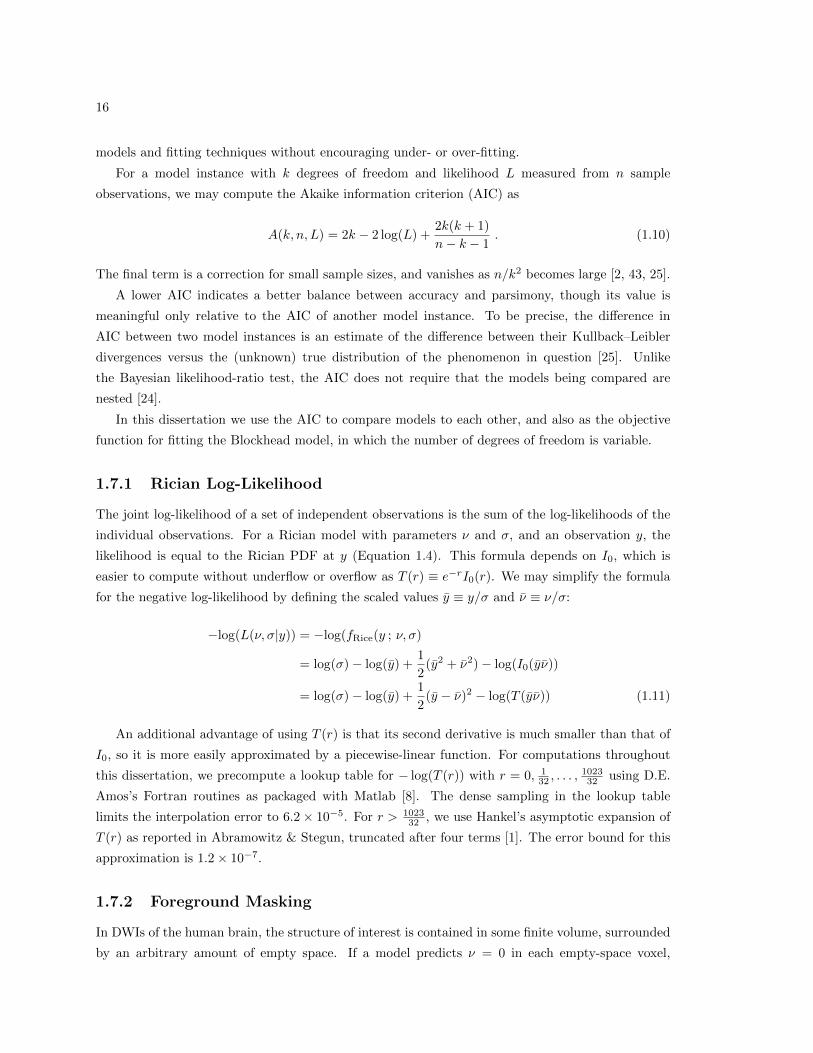
The final term is a correction for small sample sizes, and vanishes as n/k2 becomes large [2, 43, 25].

A lower AIC indicates a better balance between accuracy and parsimony, though its value is

meaningful only relative to the AIC of another model instance. To be precise, the difference in

AIC between two model instances is an estimate of the difference between their Kullback–Leibler

divergences versus the (unknown) true distribution of the phenomenon in question [25]. Unlike

the Bayesian likelihood-ratio test, the AIC does not require that the models being compared are

nested [24].

In this dissertation we use the AIC to compare models to each other, and also as the objective

function for fitting the Blockhead model, in which the number of degrees of freedom is variable.

1.7.1 Rician Log-Likelihood

The joint log-likelihood of a set of independent observations is the sum of the log-likelihoods of the

individual observations. For a Rician model with parameters ν and σ, and an observation y, the

likelihood is equal to the Rician PDF at y (Equation 1.4). This formula depends on I0, which is

easier to compute without underflow or overflow as T (r) ≡ e−rI0(r). We may simplify the formula

for the negative log-likelihood by defining the scaled values y ≡ y/σ and ν ≡ ν/σ:

−log(L(ν, σ|y)) = −log(fRice(y ; ν, σ)

= log(σ)− log(y) +1

2(y2 + ν2)− log(I0(yν))

= log(σ)− log(y) +1

2(y − ν)2 − log(T (yν)) (1.11)

An additional advantage of using T (r) is that its second derivative is much smaller than that of

I0, so it is more easily approximated by a piecewise-linear function. For computations throughout

this dissertation, we precompute a lookup table for − log(T (r)) with r = 0, 132 , . . . ,

102332 using D.E.

Amos’s Fortran routines as packaged with Matlab [8]. The dense sampling in the lookup table

limits the interpolation error to 6.2× 10−5. For r > 102332 , we use Hankel’s asymptotic expansion of

T (r) as reported in Abramowitz & Stegun, truncated after four terms [1]. The error bound for this

approximation is 1.2× 10−7.

1.7.2 Foreground Masking

In DWIs of the human brain, the structure of interest is contained in some finite volume, surrounded

by an arbitrary amount of empty space. If a model predicts ν = 0 in each empty-space voxel,

17

the expected value of the negative log-likelihood for each observation is (log(σ2/2) + 2 + γ)/2 ≈log(σ) + 0.942, where γ is the Euler-Mascheroni constant.

If there were N acquisitions (distinct DWIs) in the input, increasing the number of empty voxels

by ∆e would increase the −2 log(L) term of the AIC by about N∆e · (2 log(σ) + 1.884) regardless of

model. Many models (such as DT and CSD) use a fixed number of model parameters in each voxel,

regardless of the structure there. For these models, increasing the number of empty voxels by ∆e

would also drive up the 2k term (for example, by 14∆e in the DT model). The Blockhead model,

on the other hand, uses no parameters to represent empty voxels, so the 2k term would remain

the same. (The correction term for DT’s AIC would also grow relative to the correction term for

Blockhead.) Therefore one could easily manipulate the results of an AIC comparison to favor the

Blockhead model, simply by increasing the imaging volume to include more empty voxels.

To protect against this effect, we assume that every input image is accompanied by a “foreground

mask” that excludes all but a small number of empty voxels. (The excluded empty voxels are used

to estimate σ as in §1.6.1.) In all comparison between model instances in the evaluation sections

of this dissertation, we compute the AIC only over the set of voxels marked as foreground by this

mask.

However, the optimization processes described in §2.2.4 and §3.2 also involve computing the AIC

for various alternative instances of the Blockhead model. For these AIC computations, we include

in the foreground set all additional voxels that overlap with foreground tissue structures explicitly

represented by the model instance itself. Otherwise, two model instances that are identical in the

masked foreground would be indistinguishable to the optimzation algorithm, even if one of them

included spurious structures outside of the mask.

18

Chapter 2

The “Blockhead” Model of White-

Matter Structure

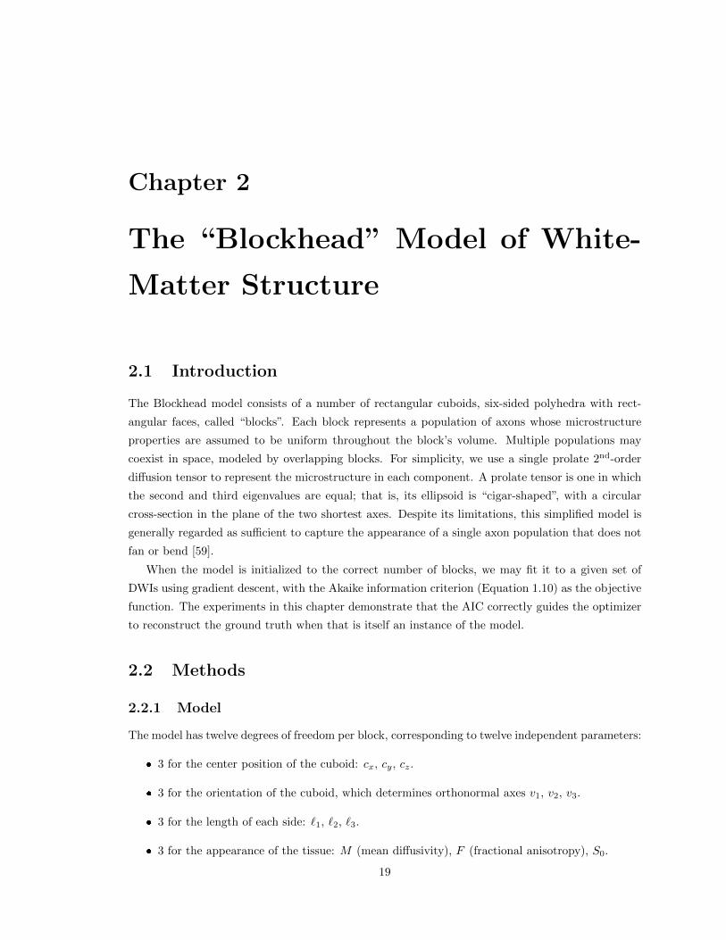
2.1 Introduction

The Blockhead model consists of a number of rectangular cuboids, six-sided polyhedra with rect-

angular faces, called “blocks”. Each block represents a population of axons whose microstructure

properties are assumed to be uniform throughout the block’s volume. Multiple populations may

coexist in space, modeled by overlapping blocks. For simplicity, we use a single prolate 2nd-order

diffusion tensor to represent the microstructure in each component. A prolate tensor is one in which

the second and third eigenvalues are equal; that is, its ellipsoid is “cigar-shaped”, with a circular

cross-section in the plane of the two shortest axes. Despite its limitations, this simplified model is

generally regarded as sufficient to capture the appearance of a single axon population that does not

fan or bend [59].

When the model is initialized to the correct number of blocks, we may fit it to a given set of

DWIs using gradient descent, with the Akaike information criterion (Equation 1.10) as the objective

function. The experiments in this chapter demonstrate that the AIC correctly guides the optimizer

to reconstruct the ground truth when that is itself an instance of the model.

2.2 Methods

2.2.1 Model

The model has twelve degrees of freedom per block, corresponding to twelve independent parameters:

� 3 for the center position of the cuboid: cx, cy, cz.

� 3 for the orientation of the cuboid, which determines orthonormal axes v1, v2, v3.

� 3 for the length of each side: `1, `2, `3.

� 3 for the appearance of the tissue: M (mean diffusivity), F (fractional anisotropy), S0.

19

20

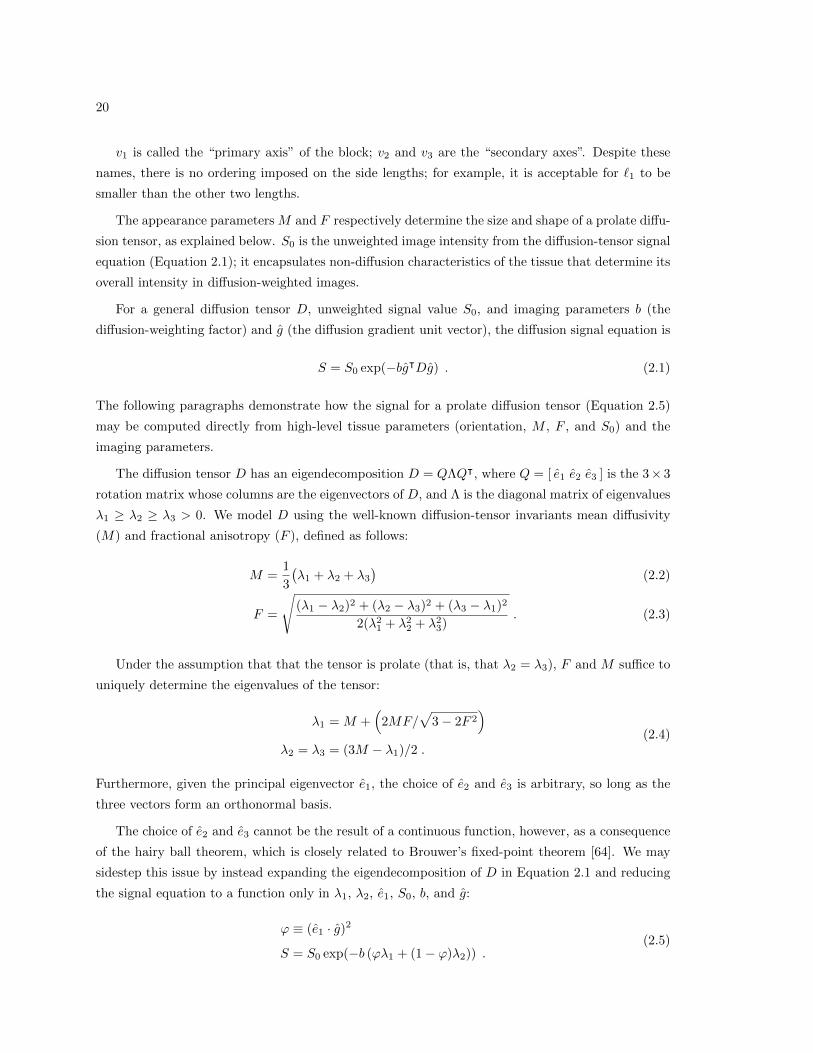
v1 is called the “primary axis” of the block; v2 and v3 are the “secondary axes”. Despite these

names, there is no ordering imposed on the side lengths; for example, it is acceptable for `1 to be

smaller than the other two lengths.

The appearance parameters M and F respectively determine the size and shape of a prolate diffu-

sion tensor, as explained below. S0 is the unweighted image intensity from the diffusion-tensor signal

equation (Equation 2.1); it encapsulates non-diffusion characteristics of the tissue that determine its

overall intensity in diffusion-weighted images.

For a general diffusion tensor D, unweighted signal value S0, and imaging parameters b (the

diffusion-weighting factor) and g (the diffusion gradient unit vector), the diffusion signal equation is

S = S0 exp(−bgᵀDg) . (2.1)

The following paragraphs demonstrate how the signal for a prolate diffusion tensor (Equation 2.5)

may be computed directly from high-level tissue parameters (orientation, M , F , and S0) and the

imaging parameters.

The diffusion tensor D has an eigendecomposition D = QΛQᵀ, where Q = [ e1 e2 e3 ] is the 3× 3

rotation matrix whose columns are the eigenvectors of D, and Λ is the diagonal matrix of eigenvalues

λ1 ≥ λ2 ≥ λ3 > 0. We model D using the well-known diffusion-tensor invariants mean diffusivity

(M) and fractional anisotropy (F ), defined as follows:

M =1

3

(λ1 + λ2 + λ3

)(2.2)

F =

√(λ1 − λ2)2 + (λ2 − λ3)2 + (λ3 − λ1)2

2(λ21 + λ22 + λ23). (2.3)

Under the assumption that that the tensor is prolate (that is, that λ2 = λ3), F and M suffice to

uniquely determine the eigenvalues of the tensor:

λ1 = M +(

2MF/√

3− 2F 2)

λ2 = λ3 = (3M − λ1)/2 .(2.4)

Furthermore, given the principal eigenvector e1, the choice of e2 and e3 is arbitrary, so long as the

three vectors form an orthonormal basis.

The choice of e2 and e3 cannot be the result of a continuous function, however, as a consequence

of the hairy ball theorem, which is closely related to Brouwer’s fixed-point theorem [64]. We may

sidestep this issue by instead expanding the eigendecomposition of D in Equation 2.1 and reducing

the signal equation to a function only in λ1, λ2, e1, S0, b, and g:

ϕ ≡ (e1 · g)2

S = S0 exp(−b (ϕλ1 + (1− ϕ)λ2)) .(2.5)

21

Therefore, for each block in the model, it suffices to know a fiber orientation unit vector e1, the

unitless scalar F , the scalar M with units mm2/s, and the unweighted signal value S0, also a unitless

scalar. As an additional simplification of the model, we assume that e1 = v1; that is, the tissue

inside each block is oriented along the block’s primary axis. Again, note that while the eigenvalues

are numbered by decreasing magnitude, no such ordering is assumed about the values of the lengths

of the block.

Computationally, a model instance containing K blocks is represented by a list B[0 . . .K − 1] of

block objects, each of which has an attribute for each of the 12 parameters above.

We assume that the signals produced by overlapping blocks are purely additive. This is equiv-

alent to assuming that there is no exchange between the tissue compartments represented by the

overlapping blocks. In addition, this signal model (both the additivity assumption and the use of a

prolate diffusion tensor in each block) disregards several other higher-order effects in regions with

multiple fiber populations. A more detailed model that represented tissue microstructure directly

would need to account for the interactions between number of concurrent fiber populations, fiber-

crossing angle, axon caliber, extracellular volume fraction, and extracellular diffusion tortuosity. All

of these details are ignored in the present work.

2.2.2 Rendering

In order to evaluate a model instance’s fit to a given dataset, we must determine its predictions of

DWI intensities in each voxel. We developed a GPU-accelerated procedure for quickly rendering

synthetic DWIs from Blockhead instances containing tens of thousands of blocks, derived from the

“slicemap” method of Eisemann and Decoret [30].

There are three basic steps of our procedure; in each one, the GPU works in parallel over

the cartesian product of two index sets. The index i enumerates the K blocks, j enumerates the

N acquisitions, and p enumerates all the voxels in the imaged volume. Along with a Blockhead

instance, the acquisition parameters bj and gj are provided as input, and the result is a set of N

synthetic DWIs. The three steps are:

1. For each (i, p), compute Opi, the proportion of the volume of voxel p that lies inside block B[i].

2. For each (i, j), compute Sij , the signal intensity of B[i] in acquisition j, from Equation 2.5.

3. For each (p, j), compute Spj , the appearance of the DWI, as Spj =∑i

OpiSij .

To compute fractional-valued overlap values Opi, the first step supersamples the render volume

by a fixed magnification factor in each dimension. As a consequence, the Opi are quantized. We

standardize the present work on a magnification factor of 4, giving 65 possible overlap values: 0 to 1,

in steps of 164 .

22

2.2.3 Computing the AIC

Given a set of N input DWIs, along with the imaging parameters that produced them (bj and gj

for j = 0 . . . N − 1), we wish to evaluate how well some Blockhead instance predicts these observed

images. The method of our evaluation is the Akaike information criterion, or AIC.

If we consider only voxel p of acquisition j in isolation, there is a noisy observed signal value ypj at

this location in the input DWIs, and the model predicts the underlying noise-free signal as Spj . For

the purpose of computing the likelihood here, ν = Spj and we assume that σ is known (cf. §1.6.1).

The number of model degrees of freedom is k = 12K, giving an overall objective value of

A = 2k − 2

∑j

∑p

log(L(Spj , σ|ypj))

+2k(k + 1)

n− k − 1. (2.6)

As explained in §1.7.2, the voxels p under consideration are only those marked as foreground by

the input mask, or that overlap with one or more blocks. We designate the number of foreground

voxels as P ≡∑

p 1, and therefore the number of observations is n = NP .

2.2.4 Numerical Optimization

We wish to determine a Blockhead instance that minimizes the AIC for a given input set of DWIs.

For simplicity, let us assume for now that we know K, the correct number of blocks to represent

the structure under consideration.1 Then each model instance is a point in a high-dimensional

continuous parameter space, over which we seek the global minimum of an objective function f (the

AIC). The search space has 13K dimensions, as explained at the end of this section.

The standard approach for such a problem is gradient descent, or some variation on it; this will

at least find a local minimum. Variants of gradient descent generally consist of two stages, repeated

alternately until convergence. In each iteration, we have a current candidate model instance x.

The first stage is direction-picking, in which a vector v is chosen as the search direction. Second is

line-searching, in which we evaluate f(x+ αv) for some values α, searching for smaller values of f .

Eventually we settle on a desirable value for α, update the candidate instance to x+αv, and return

to the direction-picking stage. We will call one direction-picking step, followed by one line search,

an “adjustment iteration” in this and subsequent chapters.

Line-searching typically involves two sub-stages: exponentially growing α until the evaluated

points bracket a minimum on the line, followed by a search for the minimum within the bracket. In

particular, we initialize α to 0.25 (see below) and search for a bracket by multiplying or dividing it

by the golden ratio. We then subdivide the bracketed interval by the golden ratio, analogously to

binary search, as motivated in Numerical Recipes [78].

Because we do not have a closed form for f in terms of the model parameters, we cannot com-

pute the gradient directly. Furthermore, every objective-function evaluation is relatively expensive;

1The next chapter deals with estimating the correct number of blocks during fitting.

23

despite the GPU-accelerated rendering and careful pruning of unnecessary renders in unchanged

subvolumes, the function still takes on the order of 0.1 s to compute on average. Therefore it is

advantageous to be conservative with the number of function evaluations during optimization.

Rather than estimating the gradient over all 13K dimensions in each direction-picking stage, we

instead select a random block and compute the gradient over a random subset of the dimensions

corresponding to that block’s parameters. In addition, we save function evaluations by using only

a two-point estimate of the partial derivative in each dimension, when possible. On average, we

estimate the derivative in 6.5 dimensions, and do only 1.5 new function evaluations per estimate,

for a total of 9.75 expected function evaluations per estimate of the gradient.

In the line-search stage, we negate and normalize the estimated gradient, and then limit our-

selves to a budget of 6 additional function evaluations. This restricts the total distance (in the

parameterized search space) between any consecutive pair of model instances to 0.25ϕ6 ≈ 4.5.

Limiting the distance traveled in any single line search is important, in order to prevent any

single block from “outpacing” the others. It also naıvely approximates the benefits of conjugate-

gradient optimization. If every iteration reached a minimum in the line-search step, then the gradient

at that minimum, and therefore the next line-search direction, would be orthogonal to the line.

This situation would result in a zigzagging sequence of short steps with high total length, and the

pathological cases that cause this behavior become more likely as the dimensionality of the search

space increases [78]. By instead holding back from aggressively minimizing in each line-search step,

we allow the optimization to correct its search direction more frequently, and avoid wasting additional

function evaluations on small improvements early in the optimization.

Search Dimensions

Because of the quantization of the overlap values Opi at 4Ö magnification, it is possible to translate

an axis-aligned block by up to 1⁄4 of a voxel width in a single dimension without changing the

synthetic DWIs. Therefore the optimizer works in units of voxel widths, and treats 0.25 as the

natural scale of the search space. The “center position” and “side length” model parameters are

correctly scaled to this size, but the other parameters need to be manipulated for correct scaling.

In addition, it is preferable that our search space be infinite in each dimension, but some model

parameters have limited ranges. Therefore we define seven specialized optimization parameters, each

with a transformation that maps the search domain (−∞,∞) to the correct range, with a scaling

that is appropriate for the corresponding model parameter. The transformations are summarized in

Table 2.1. The optimization parameters m, f , and s respectively correspond to the mean diffusivity

M , the fractional anisotropy F , and the unweighted signal S0.

The orientation of the block has three degrees of freedom, but there are many ways to param-

eterize an orientation. We opt to use a unit quaternion, which has the advantage over, e.g., Euler

angles that it avoids gimbal lock: the effect of a small change in any single component of a unit

quaternion is fairly consistent regardless of the values of the other parameters [86, 87]. There are

four corresponding optimization parameters, the components of a quaternion q: q = 〈qx, qy, qz, qw〉.

24

(a) Singleton. (b) 90° cross. (c) 60° cross.

(d) 30° cross. (e) 3-way cross (“3X”).

(f) Cylinder. (g) Horseshoe (“U”). (h) Torus.

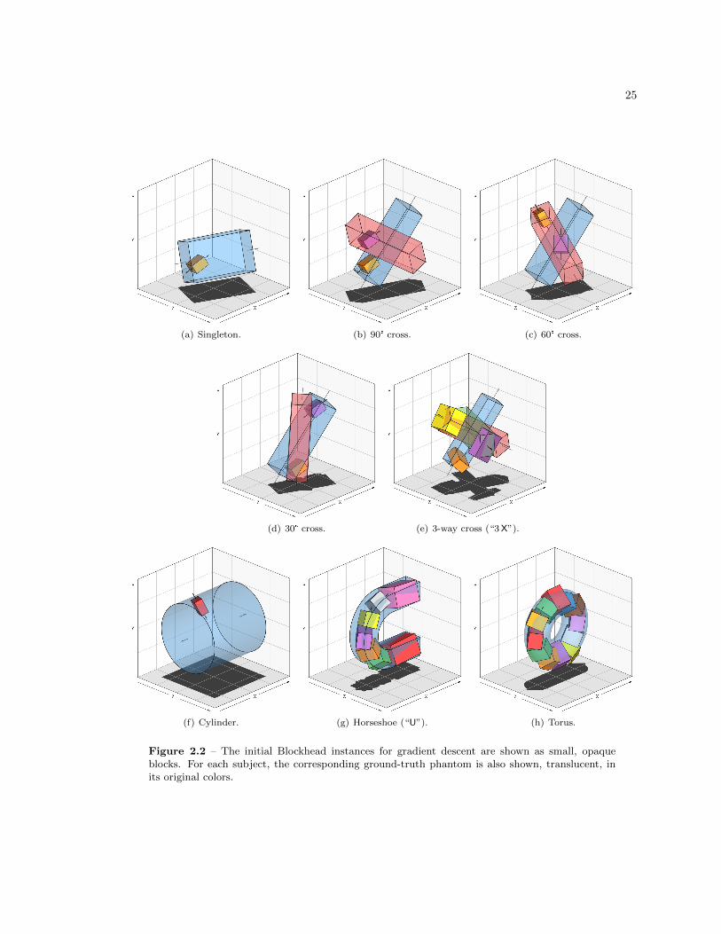
Figure 2.1 – The eight computational phantoms used in this evaluation. The different colors serveonly to distinguish the components. Black arrows extending off the ends indicate the fiber direction;for the horseshoe and torus phantoms, the fibers are oriented along the long, bending axis of theshape. (a)–(e) are instances of the Blockhead model, while (f)–(h) have curving geometry thatcannot be expressed by Blockhead. Note that the volume of the cylinder is approximately 3 timesthe total volume of any other phantom.

25

(a) Singleton. (b) 90° cross. (c) 60° cross.

(d) 30° cross. (e) 3-way cross (“3X”).

(f) Cylinder. (g) Horseshoe (“U”). (h) Torus.

Figure 2.2 – The initial Blockhead instances for gradient descent are shown as small, opaqueblocks. For each subject, the corresponding ground-truth phantom is also shown, translucent, inits original colors.

26

Transformation Mapping around typical values Range

M = m2/220 m = 22.9± 0.25 →M ≈ 0.000500± 0.000011 M ∈ [0,∞)

F = f2/(128 + f2) f = 11.3± 0.25 → F ≈ 0.5± 0.01 F ∈ [0, 1)

S0 = s2/256 s = 277± 0.25 → S0 ≈ 300± 0.5 S0 ∈ [0,∞)

Q = q/32 [See body text]

Table 2.1 – Model parameters (capital letters) and their mappings from optimization parameters(lowercase letters). Each transformation is designed so that the domain (set of possible values ofthe optimization parameter) is (−∞,∞), while the entire range is valid for the model parameter.Furthermore, near optimization parameter values that correspond to typical values in the modelparameter, a change of ±0.25 in the optimization parameter results in a fine-grained change in themodel parameter scaled appropriately to that parameter’s common range of values.

We set Q = q/32 to compute the model quaternion, and finally normalize Q before computing the

block’s coordinate frame from it. A change of 0.25 to any one of qx, qy, qz, or qw changes the block’s

orientation by about 0.5–1°.

Although the model has 12 degrees of freedom per block, since we encode the orientation using

four parameters, the search space has 13 dimensions per block.

2.3 Evaluation

Since the fitting method described so far assumes that the number of blocks is known, our evaluation

was conducted on synthetic images of eight computational phantoms with simple geometry (see

Figure 2.1):

� One Blockhead instance consisting of a single block at an oblique orientation.

� Three Blockhead instances with two blocks in each, crossing at 90°, 60°, and 30° respectively.

Note in the figure that no pair of sides from different blocks is parallel.

� One Blockhead instance with three orthogonal crossing blocks (with non-parallel orientations).

� Three non-Blockhead computational phantoms: a cylinder, a “horseshoe” (U-shaped bar with

square cross-section), and a torus. The fiber orientation within each phantom is aligned with

the primary axis of the shape.

For all of these phantoms, the ground-truth microstructure parameters are F = 0.7, M =

0.0007 mm2/s, and S0 = 290. We generated a total of 80 synthetic diffusion MRI datasets: for

each phantom, all combinations of five noise levels (σ ∈ {5, 10, 14.5, 19.3, 29}) and two non-zero

b-values (b ∈ {1000 s/mm2, 3000 s/mm2}). In each dataset, there were 10 unweighted (b = 0 s/mm2)

images and 64 diffusion-weighted images with distinct diffusion-weighting directions (determined by

an electrostatic repulsion simulation). Voxels were nominally 1 mm isotropic, with 32Ö32Ö32 voxels

in the imaging volume.

27

b = 0 b = 1000 b = 3000⊥ ‖ ⊥ ‖ ⊥ ‖

Signal (S) : 290 290 203.3 72.3 99.9 4.49

SNR @ σ =

5.0 : 58 58 40.7 14.5 20.0 0.90

10.0 : 29 29 20.3 7.2 10.0 0.4514.5 : 20 20 14.0 5.0 6.9 0.3119.3 : 15 15 10.5 3.7 5.2 0.2329.0 : 10 10 7.0 2.5 3.4 0.15

Table 2.2 – SNR at various noise levels, for synthetic tissue with S0 = 290, M = 0.0007 mm2/s,

F = 0.7. The columns labeled “⊥” are for diffusion signals measured perpendicular to the fiberorientation; “‖” means parallel to the fiber orientation.

To evaluate sensitivity to noise, we also generated noise-free (σ = 0) synthetic DWIs of each

phantom for each b-value.

Since SNR is a more familiar, albeit less useful, measure of noise than σ (see §1.6), Table 2.2

summarizes the equivalent SNR for these synthetic datasets in DWIs where g is perpendicular or

parallel to the fiber orientation, at all three relevant b-values.

2.3.1 Model-Instance Comparison

Established Models

To provide a baseline of comparison, we fit two well-established models from the literature to each

dataset. First, we used Wang, et al.’s Diffusion Toolkit software to fit diffusion tensors [97]. Second,

we used constrained spherical deconvolution, as implemented in Tournier, et al.’s MRtrix software,

to estimate the fiber orientation distribution function in each voxel [92, 93] We will refer to these

models, respectively, as “DT” and “CSD”. Both these models fit a single mathematical object (tensor

or orientation distribution) in each voxel. However, the single orientation distribution computed by

CSD in each voxel may have multiple peaks, representing multiple fiber populations in that voxel.

In order to predict signal values, the DT model requires 7 degrees of freedom per voxel: one for

S0 and six for the tensor itself. For the CSD model, we set the harmonic order lmax = 4, which

is standard for typical acquisitions [92]. At this harmonic order, the CSD model has 4 degrees of

freedom to represent the single-fiber signal profile, plus 29 degrees of freedom per voxel: one for S0,

and 1 + 5 + 9 + 13 = 28 for even spherical harmonic amplitudes of the fiber orientation distribution.

Oracle Instances

The first five phantoms are themselves instances of the Blockhead model. We constructed “oracle

fits” for these subjects simply by duplicating the ground-truth instances. These represent the best

possible fit achievable for the Blockhead model, and are elements of the feasible search space for

28

Single 90° 60° 30° 3X Cyl U Torus

# vox (P ) 3666 4027 3889 3353 3466 11416 3332 4440# obs (n) 271284 297998 287786 248122 256484 844784 246568 328560DT df (k) 25662 28189 27223 23471 24262 79912 23324 31080

CSD df (k) 102652 112760 108896 93888 97052 319652 93300 124324BH df (k) 12 24 24 24 36 12 84 144

Table 2.3 – Basic measures of the experimental subjects. The variable names given in the firstcolumn are discussed in §1.7 and §2.2.3. P is the number of foreground voxels; n = PN is the totalnumber of observations, where N = 74 for every acquisition. The final rows show the number ofmodel degrees of freedom (k) for DT, CSD, and the Blockhead instances fit by gradient descent.

any fitting method. Therefore they provide an additional baseline for comparison to automatically-

generated fits.

Gradient-Descent Fit

We ran the gradient-descent optimizer on datasets for all eight test subjects at both b-values and noise

levels 14.5 and 29. For the first five subjects (whose underlying structures are Blockhead instances),

we initialized the optimizer with the correct number of blocks. Each initial block partially overlapped

a corresponding block in the ground truth, but was oblique to it and much smaller, with an average

edge length of 4.5 mm.

The initial instance for the cylinder subject was also a single small block, overlapping with

the cylinder but oblique to it. For the other three subjects, the initial instances were hand-built

arrangements of blocks that roughly matched the shaped of the target structure. For the horseshoe,

we used seven initial blocks; for the torus, 12 blocks. See Figure 2.2 for pictures of the initial states

relative to the ground truth.

The appearance parameters for all initial blocks were S0 = 318, M = 0.0011 mm2/s, and F = 0.5.

2.4 Results and Discussion

2.4.1 DT vs. CSD

For every tested dataset, the difference in AIC values between CSD and DT fits is positive (Fig-

ure 2.3(a)). These results indicate that DT provides a more informative fit than CSD. DT’s advan-

tage over CSD narrows under particular circumstances: datasets containing fibers crossing at large

angles, imaged with low noise and high b-values.

The AIC balances model accuracy (measured by negative log-likelihood, −log(L)) against par-

simony (measured by the terms involving degrees of freedom and sample counts, k and n). Smaller

values of −log(L) indicate a more accurate fit. As discussed in §1.7.1, the joint log-likelihood of an

entire model instance is the sum of the log-likelihood for each observation: each signal measurement

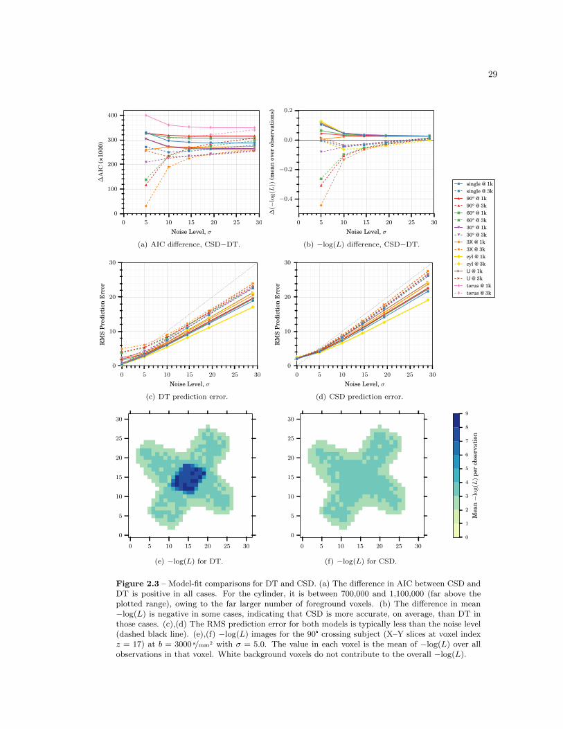
29

0 5 10 15 20 25 30

Noise Level, σ

0

100

200

300

400

∆A

IC�(�×

�1�0�0�0

�)

single @ 1ksingle @ 3k�9�0�° @ 1k�9�0�° @ 3k�6�0�° @ 1k�6�0�° @ 3k�3�0�° @ 1k�3�0�° @ 3k3X @ 1k3X @ 3kcyl @ 1kcyl @ 3kU @ 1kU @ 3ktorus @ 1ktorus @ 3k

(a) AIC difference, CSD−DT.

0 5 10 15 20 25 30

Noise Level, σ

−0.4

−0.2

0.0

0.2

∆(−

log(L

))(m

ean

over

obse

rvat

ions

)

single @ 1ksingle @ 3k�9�0�° @ 1k�9�0�° @ 3k�6�0�° @ 1k�6�0�° @ 3k�3�0�° @ 1k�3�0�° @ 3k3X @ 1k3X @ 3kcyl @ 1kcyl @ 3kU @ 1kU @ 3ktorus @ 1ktorus @ 3k

(b) −log(L) difference, CSD−DT.

0 5 10 15 20 25 30

Noise Level, σ

0

100

200

300

400

∆A

IC�(�×

�1�0�0�0

�)

single @ 1ksingle @ 3k�9�0�° @ 1k�9�0�° @ 3k�6�0�° @ 1k�6�0�° @ 3k�3�0�° @ 1k�3�0�° @ 3k3X @ 1k3X @ 3kcyl @ 1kcyl @ 3kU @ 1kU @ 3ktorus @ 1ktorus @ 3k

0 5 10 15 20 25 30

Noise Level, σ

0

10

20

30

RM

SP

redi

ctio

nE

rror

single @ 1ksingle @ 3k�9�0�° @ 1k�9�0�° @ 3k�6�0�° @ 1k�6�0�° @ 3k�3�0�° @ 1k�3�0�° @ 3k3X @ 1k3X @ 3kcyl @ 1kcyl @ 3kU @ 1kU @ 3ktorus @ 1ktorus @ 3k

(c) DT prediction error.

0 5 10 15 20 25 30

Noise Level, σ

0

10

20

30

RM

SP

redi

ctio

nE

rror

single @ 1ksingle @ 3k�9�0�° @ 1k�9�0�° @ 3k�6�0�° @ 1k�6�0�° @ 3k�3�0�° @ 1k�3�0�° @ 3k3X @ 1k3X @ 3kcyl @ 1kcyl @ 3kU @ 1kU @ 3ktorus @ 1ktorus @ 3k

(d) CSD prediction error.

0 5 10 15 20 25 30

0

5

10

15

20

25

30

0

1

2

3

4

5

6

7

8

9

Mea

n−l

og(L

)pe

rob

serv

atio

n

(e) −log(L) for DT.

0 5 10 15 20 25 30

0

5

10

15

20

25

30

0

1

2

3

4

5

6

7

8

9

Mea

n−l

og(L

)pe

rob

serv

atio

n

(f) −log(L) for CSD.

0 5 10 15 20 25 30

0

5

10

15

20

25

30

0

1

2

3

4

5

6

7

8

9

Mea

n−l

og(L

)pe

rob

serv

atio

n

Figure 2.3 – Model-fit comparisons for DT and CSD. (a) The difference in AIC between CSD andDT is positive in all cases. For the cylinder, it is between 700,000 and 1,100,000 (far above theplotted range), owing to the far larger number of foreground voxels. (b) The difference in mean−log(L) is negative in some cases, indicating that CSD is more accurate, on average, than DT inthose cases. (c),(d) The RMS prediction error for both models is typically less than the noise level(dashed black line). (e),(f) −log(L) images for the 90° crossing subject (X–Y slices at voxel indexz = 17) at b = 3000 s/mm2 with σ = 5.0. The value in each voxel is the mean of −log(L) over allobservations in that voxel. White background voxels do not contribute to the overall −log(L).

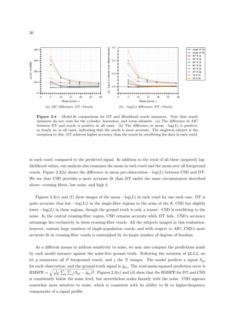
30

0 5 10 15 20 25 30

Noise Level, σ

0

100

200

300

400

∆A

IC�(�×

�1�0�0�0

�)

single @ 1ksingle @ 3k�9�0�° @ 1k�9�0�° @ 3k�6�0�° @ 1k�6�0�° @ 3k�3�0�° @ 1k�3�0�° @ 3k3X @ 1k3X @ 3k

(a) AIC difference, DT−Oracle.

0 5 10 15 20 25 30

Noise Level, σ

0.0

0.2

0.4

0.6

∆(−

log(L

))(m

ean

over

obse

rvat

ions

)

single @ 1ksingle @ 3k�9�0�° @ 1k�9�0�° @ 3k�6�0�° @ 1k�6�0�° @ 3k�3�0�° @ 1k�3�0�° @ 3k3X @ 1k3X @ 3k

(b) −log(L) difference, DT−Oracle.

0 5 10 15 20 25 30

Noise Level, σ

0

100

200

300

400

∆A

IC�(�×

�1�0�0�0

�)

single @ 1ksingle @ 3k�9�0�° @ 1k�9�0�° @ 3k�6�0�° @ 1k�6�0�° @ 3k�3�0�° @ 1k�3�0�° @ 3k3X @ 1k3X @ 3k

Figure 2.4 – Model-fit comparisons for DT and Blockhead oracle instances. Note that oracleinstances do not exist for the cylinder, horseshoe, and torus datasets. (a) The difference in AICbetween DT and oracle is positive in all cases. (b) The difference in mean −log(L) is positive,or nearly so, in all cases, indicating that the oracle is more accurate. The singleton subject is theexception to this: DT achieves higher accuracy than the oracle by overfitting the data in each voxel.

in each voxel, compared to the predicted signal. In addition to the total of all these (negated) log-

likelihood values, our analysis also examines the mean in each voxel and the mean over all foreground

voxels. Figure 2.3(b) shows the difference in mean per-observation −log(L) between CSD and DT.

We see that CSD provides a more accurate fit than DT under the same circumstances described

above: crossing fibers, low noise, and high b.

Figures 2.3(e) and (f) show images of the mean −log(L) in each voxel for one such case. DT is

quite accurate (has low −log(L)) in the single-fiber regions in the arms of the X. CSD has slightly

lower −log(L) in these regions, though the ground truth is only a tensor—CSD is overfitting to the

noise. In the central crossing-fiber region, CSD remains accurate while DT fails. CSD’s accuracy

advantage lies exclusively in these crossing-fiber voxels. All the subjects imaged in this evaluation,

however, contain large numbers of single-population voxels, and with respect to AIC, CSD’s more

accurate fit in crossing-fiber voxels is outweighed by its larger number of degrees of freedom.

As a different means to address sensitivity to noise, we may also compare the predictions made

by each model instance against the noise-free ground truth. Following the notation of §2.2.2, we

let p enumerate all P foreground voxels, and j the N images. The model predicts a signal Spj

for each observation, and the ground-truth signal is ypj . The root-mean-squared prediction error is

RMSPE =√

1PN

∑p

∑j(Spj − ypj)2. Figures 2.3(c) and (d) show that the RMSPE for DT and CSD

is consistently below the noise level, but nevertheless scales linearly with the noise. CSD appears

somewhat more sensitive to noise, which is consistent with its ability to fit to higher-frequency

components of a signal profile.

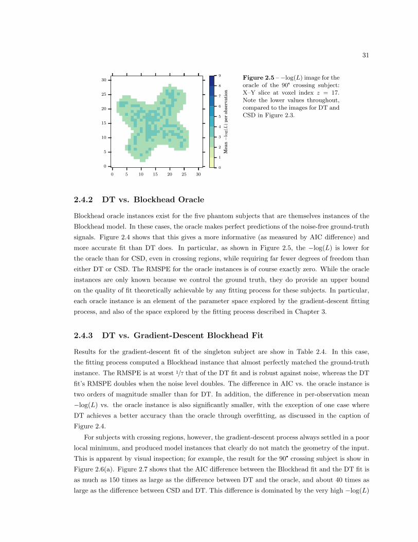
31

0 5 10 15 20 25 30

0

5

10

15

20

25

30

0

1

2

3

4

5

6

7

8

9

Mea

n−l

og(L

)pe

rob

serv

atio

n

Figure 2.5 – −log(L) image for theoracle of the 90° crossing subject:X–Y slice at voxel index z = 17.Note the lower values throughout,compared to the images for DT andCSD in Figure 2.3.

2.4.2 DT vs. Blockhead Oracle

Blockhead oracle instances exist for the five phantom subjects that are themselves instances of the

Blockhead model. In these cases, the oracle makes perfect predictions of the noise-free ground-truth

signals. Figure 2.4 shows that this gives a more informative (as measured by AIC difference) and

more accurate fit than DT does. In particular, as shown in Figure 2.5, the −log(L) is lower for

the oracle than for CSD, even in crossing regions, while requiring far fewer degrees of freedom than

either DT or CSD. The RMSPE for the oracle instances is of course exactly zero. While the oracle

instances are only known because we control the ground truth, they do provide an upper bound

on the quality of fit theoretically achievable by any fitting process for these subjects. In particular,

each oracle instance is an element of the parameter space explored by the gradient-descent fitting

process, and also of the space explored by the fitting process described in Chapter 3.

2.4.3 DT vs. Gradient-Descent Blockhead Fit

Results for the gradient-descent fit of the singleton subject are show in Table 2.4. In this case,

the fitting process computed a Blockhead instance that almost perfectly matched the ground-truth

instance. The RMSPE is at worst 1/7 that of the DT fit and is robust against noise, whereas the DT

fit’s RMSPE doubles when the noise level doubles. The difference in AIC vs. the oracle instance is

two orders of magnitude smaller than for DT. In addition, the difference in per-observation mean

−log(L) vs. the oracle instance is also significantly smaller, with the exception of one case where

DT achieves a better accuracy than the oracle through overfitting, as discussed in the caption of

Figure 2.4.

For subjects with crossing regions, however, the gradient-descent process always settled in a poor

local minimum, and produced model instances that clearly do not match the geometry of the input.

This is apparent by visual inspection; for example, the result for the 90° crossing subject is show in

Figure 2.6(a). Figure 2.7 shows that the AIC difference between the Blockhead fit and the DT fit is

as much as 150 times as large as the difference between DT and the oracle, and about 40 times as

large as the difference between CSD and DT. This difference is dominated by the very high −log(L)

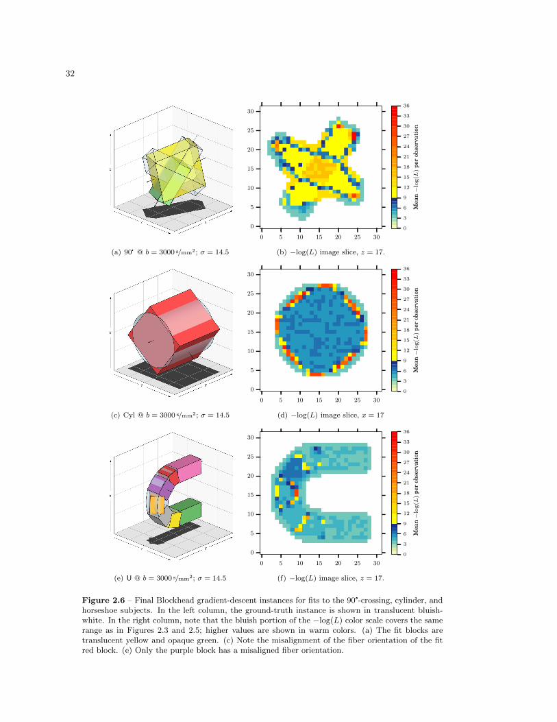
32

(a) 90° @ b = 3000 s/mm2; σ = 14.5

0 5 10 15 20 25 30

0

5

10

15

20

25

30

0

3

6

9

12

15

18

21

24

27

30

33

36

Mea

n−l

og(L

)pe

rob

serv

atio

n

(b) −log(L) image slice, z = 17.

(c) Cyl @ b = 3000 s/mm2; σ = 14.5

0 5 10 15 20 25 30

0

5

10

15

20

25

30

0

3

6

9

12

15

18

21

24

27

30

33

36

Mea

n−l

og(L

)pe

rob

serv

atio

n(d) −log(L) image slice, x = 17

(e) U @ b = 3000 s/mm2; σ = 14.5

0 5 10 15 20 25 30

0

5

10

15

20

25

30

0

3

6

9

12

15

18

21

24

27

30

33

36

Mea

n−l

og(L

)pe

rob

serv

atio

n

(f) −log(L) image slice, z = 17.

Figure 2.6 – Final Blockhead gradient-descent instances for fits to the 90°-crossing, cylinder, andhorseshoe subjects. In the left column, the ground-truth instance is shown in translucent bluish-white. In the right column, note that the bluish portion of the −log(L) color scale covers the samerange as in Figures 2.3 and 2.5; higher values are shown in warm colors. (a) The fit blocks aretranslucent yellow and opaque green. (c) Note the misalignment of the fiber orientation of the fitred block. (e) Only the purple block has a misaligned fiber orientation.

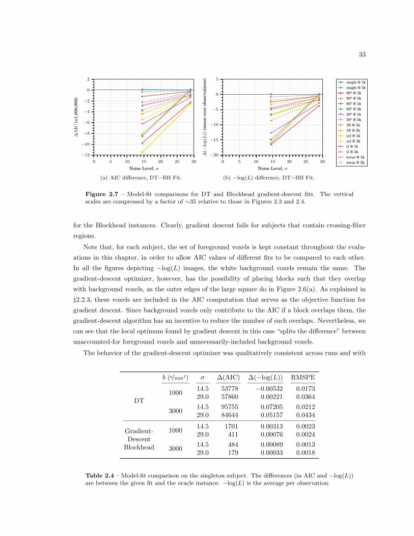
33

0 5 10 15 20 25 30

Noise Level, σ

−12

−10

−8

−6

−4

−2

0

2∆

AIC

�(��1�,

�0�0�0�,

�0�0�0�)

single @ 1ksingle @ 3k�9�0�° @ 1k�9�0�° @ 3k�6�0�° @ 1k�6�0�° @ 3k�3�0�° @ 1k�3�0�° @ 3k3X @ 1k3X @ 3kcyl @ 1kcyl @ 3kU @ 1kU @ 3ktorus @ 1ktorus @ 3k

(a) AIC difference, DT−BH Fit.

0 5 10 15 20 25 30

Noise Level, σ

−20

−15

−10

−5

0

5

∆(−

log(L

))(m

ean

over

obse

rvat

ions

)

single @ 1ksingle @ 3k�9�0�° @ 1k�9�0�° @ 3k�6�0�° @ 1k�6�0�° @ 3k�3�0�° @ 1k�3�0�° @ 3k3X @ 1k3X @ 3kcyl @ 1kcyl @ 3kU @ 1kU @ 3ktorus @ 1ktorus @ 3k

(b) −log(L) difference, DT−BH Fit.

0 5 10 15 20 25 30

Noise Level, σ

−12

−10

−8

−6

−4

−2

0

2

∆A

IC�(�×

�1�,�0�0

�0�,�0�0

�0�)

single @ 1ksingle @ 3k�9�0�° @ 1k�9�0�° @ 3k�6�0�° @ 1k�6�0�° @ 3k�3�0�° @ 1k�3�0�° @ 3k3X @ 1k3X @ 3kcyl @ 1kcyl @ 3kU @ 1kU @ 3ktorus @ 1ktorus @ 3k

Figure 2.7 – Model-fit comparisons for DT and Blockhead gradient-descent fits. The verticalscales are compressed by a factor of ∼35 relative to those in Figures 2.3 and 2.4.

for the Blockhead instances. Clearly, gradient descent fails for subjects that contain crossing-fiber

regions.

Note that, for each subject, the set of foreground voxels is kept constant throughout the evalu-

ations in this chapter, in order to allow AIC values of different fits to be compared to each other.

In all the figures depicting −log(L) images, the white background voxels remain the same. The

gradient-descent optimizer, however, has the possibility of placing blocks such that they overlap

with background voxels, as the outer edges of the large square do in Figure 2.6(a). As explained in

§2.2.3, these voxels are included in the AIC computation that serves as the objective function for

gradient descent. Since background voxels only contribute to the AIC if a block overlaps them, the

gradient-descent algorithm has an incentive to reduce the number of such overlaps. Nevertheless, we

can see that the local optimum found by gradient descent in this case “splits the difference” between

unaccounted-for foreground voxels and unnecessarily-included background voxels.

The behavior of the gradient-descent optimizer was qualitatively consistent across runs and with

b (s/mm2) σ ∆(AIC) ∆(−log(L)) RMSPE

DT1000

14.5 53778 −0.00532 0.017329.0 57860 0.00221 0.0364

300014.5 95755 0.07205 0.021229.0 84644 0.05157 0.0434

Gradient-Descent

Blockhead

100014.5 1701 0.00313 0.002329.0 411 0.00076 0.0024

300014.5 484 0.00089 0.001329.0 179 0.00033 0.0018

Table 2.4 – Model-fit comparison on the singleton subject. The differences (in AIC and −log(L))are between the given fit and the oracle instance. −log(L) is the average per observation.

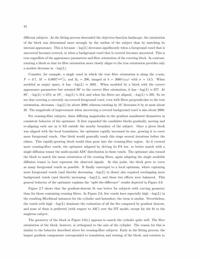
34

different subjects. As the fitting process descended the objective-function landscape, the orientation

of the block was determined more strongly by the outline of the subject than by matching its

internal appearance. This is because −log(L) decreases signifincatly when a foreground voxel that is

uncovered becomes covered, or when a background voxel that is covered becomes uncovered. This is

true regardless of the appearance parameters and fiber orientation of the covering block. In contrast,

rotating a block so that its fiber orientation more closely aligns to the true orientation provides only

a modest decrease in −log(L).

Consider, for example, a single voxel in which the true fiber orientation is along the x-axis,

F = 0.7, M = 0.0007 mm2/s, and S0 = 290, imaged at b = 3000 s/mm2 with σ = 14.5. When

modeled as empty space, it has −log(L) ≈ 2691. When modeled by a block with the correct

appearance parameters but oriented 90° to the correct fiber orientation, it has −log(L) ≈ 677. At

80°, −log(L) ≈ 674; at 10°, −log(L) ≈ 314; and when the fibers are aligned, −log(L) ≈ 295. So we

see that covering a currently un-covered foreground voxel, even with fibers perpendicular to the true

orientation, decreases −log(L) by about 2000, whereas rotating by 10° decreases it by at most about

20. The magnitude of improvement when uncovering a covered background voxel is also about 2000.

For crossing-fiber subjects, these differing magnitudes in the gradient manifested themselves in

consistent behavior of the optimizer. It first expanded the candidate blocks gradually, moving and

re-aligning each one as it fell outside the nearby boundary of the subject. Once a given block

was aligned with the local boundaries, the optimizer rapidly increased its size, growing it to cover

more foreground voxels. One block would generally reach this stage several iterations before the

others. This rapidly-growing block would then grow into the crossing-fiber region. As it covered

more crossing-fiber voxels, the optimizer adapted by driving its FA low, to better match with a

single diffusion tensor the multi-modal ADC distribution in these voxels. The optimizer also turned

the block to match the mean orientation of the crossing fibers, again adapting the single available

diffusion tensor to best represent the observed signals. At this point, the block grew to cover

as many foreground voxels as possible. It finally converged to a local optimum, where capturing

more foreground voxels (and thereby decreasing −log(L) in those) also required overlapping more

background voxels (and thereby increasing −log(L)), and these two effects were balanced. This

general behavior of the optimizer explains the “split-the-difference” results depicted in Figure 2.6.

Figure 2.7 shows that the gradient-descent fit was better for subjects with curving geometry

than for those containing crossing fibers. In Figure 2.6, few voxels have especially high −log(L) in

the resulting Blockhead instances for the cylinder and horseshoe; the torus is similar. Nevertheless,

the voxels with high −log(L) dominate the evaluation of all the fits computed by gradient descent,

and none of them is preferred (with respect to AIC) over the DT model, except for the fit to the

singleton subject.

The geometry of the block in Figure 2.6(c) appears to match the cylinder quite well. The fiber

orientation of the block, however, is orthogonal to the axis of the cylinder. The reason for this is

similar to the behavior described above for crossing-fiber subjects. Early in the fitting process, the

largest gradient components corresponded to translation and resizing of the block, and rotation to

35

align its outline with the outline of the subject. Once the geometry was well-aligned to that of the

subject, however, rotating the block by a small angle to better align the fiber orientation would

have incurred an enormous increase in −log(L) due to the covering effects discussed above. As a

consequence, the optimizer was stuck with misaligned fibers. In the end, the optimizer adapted

to this incorrect orientation by setting FA to 0, thereby minimizing (as best as possible) the total

inaccuracy of the signal predictions. This poor orientation match is evident in the high −log(L) in

the interior seen in Figure 2.6(d).

In all three examples displayed in Figure 2.6, the optimizer fit the outlines of the subjects quite

precisely. The teal block in (a), for example, aligns very closely to the true geometry of the subject,

even though it is oblique to the voxel grid. Similar results were achieved for the horseshoe in (e),

although its flat faces fall precisely on voxel boundaries.

2.5 Conclusions

The experimental results for Blockhead oracles show that, for synthetic subjects with rectangular

geometry, Blockhead model instances can have a far higher-quality fit (in terms both of accuracy and

parsimony) than is achievable with DT or CSD. Even subjects with curving geometry can be roughly

modeled by Blockhead instances, with inaccuracies clustered near the boundary. This suggests that

generalizations of the Blockhead model, allowing for more diverse geometry, could possibly overcome

some of the shortcomings of the current cuboid-based implementation, while still being amenable to

automatic fitting.

When initialized with the correct number of blocks, gradient descent can precisely match the

local sub-voxel geometry of the subject. It does, however, get caught in attraction basins for poor

local optima, and performs especially poorly when attempting to model subjects containing crossing

fibers.

The algorithm presented in Chapter 3 is motivated by the observations that the correct num-

ber of blocks is not, in general, known a priori, and that gradient descent alone is insufficient to

grow candidate blocks through crossing-fiber regions. This algorithm automatically fits Blockhead

model instances without knowing the number of blocks in advance. It also avoids or escapes local

minima that can trap the naıve gradient-descent optimizer, by starting with many small blocks and

progressively joining, splitting, adding, or deleting them while also adjusting their parameters.

36

Chapter 3

Discrete–Continuous Optimization

3.1 Introduction

The previous chapter discussed adjusting a Blockhead model instance when the correct number

of blocks is known. In general, however, this number must be determined as part of the fitting

process. Combinatorial optimization is the apparent discipline to consult when confronting a search

task that involves discrete values like the presence or absence of any given block. However, it is

challenging to incorporate the continuous geometry and appearance parameters of each block into

classical combinatorial-optimization strategies.

This chapter describes a method for applying local search to this mixed discrete–continuous

optimization problem. This method is compatible with standard local-search metaheuristics that

help the search reach better local optima. The experiments in this chapter demonstrate that a

fully-automatic solver can often reconstruct the ground-truth structure when this structure is an

instance of the Blockhead model. For datasets with curved geometry, the experiments reveal how

the fitting system deals with the limitations of the model.

3.2 Methods

3.2.1 Local Search Moves

As in Chapter 2, we use the Akaike information criterion (AIC; Equation 1.10) as our objective

function for optimization of Blockhead model instances. Due to the continuity properties of the

AIC, and the relatively unstructured nature of our problem otherwise, we selected local search as

our optimization strategy.

Local search iteratively explores the model space by evaluating a sequence of candidate model

instances (or optimization “states”). For a given state, a “move” is an operation that generates a

new state by modifying the old one. In any application of local search, the implementer’s primary

design decision is the selection of the set of legal moves. For the Blockhead problem, we wish to

support the following classes of moves:

37

38

� Add a block at a given location.

� Delete a set of blocks.

� Merge a set of blocks into one block.

� Split a single block in two along a plane parallel to one of its sides.

� Adjust the continuous parameters of a single block, as in Chapter 2.

Many classic combinatorial optimization problems may be usefully formulated as the selection

of an optimal subset of a finite “universe” of fixed elements. For the traveling salesperson problem,

for example, the universe is all edges of a graph; for the knapsack problem, it’s a set of items that

could go in the knapsack. The universe of the Blockhead fitting problem is therefore all possible

blocks: an infinite set. Restricting this to only those blocks that are distinguishable by our rendering

algorithm makes the universe finite, but it is still impractically large to compute.

Our solution is to instead generate elements of the universe on the fly, as they are needed for

inclusion in candidate instances. The fitting algorithm maintains an ever-growing list of immutable

blocks, which we call the “known universe”, consisting of all blocks that have ever been members of

any explored model instance. When a newly-explored state includes new blocks, these are appended

to the end of the list, so that the index of each block remains fixed once it is in the list. A given

model instance is then a subset of this known universe: blocks included in it are said to be “active”

for that instance, and the rest are “inactive”. These active blocks may be specified by a binary mask

over the known universe, called the instance’s “active list”. Implicitly, all blocks not in the known

universe are inactive for all model instances so far explored.

Moving from one state to another is therefore equivalent to copying the active list, appending

zero or more new blocks to the known universe, and modifying zero or more entries in the new active

list (“marking” blocks as active or inactive). The five moves above are implemented as follows:

� Add a block: Append this block to the known universe and mark it active.

� Delete a set of blocks: Mark them inactive.

� Merge a set of blocks: Create a new block—the result of the virtual merger. Append this

new block to the known universe, mark it active, and mark the old blocks inactive.

� Split a block: Create two new blocks—the result of the virtual split. Append them both to

the known universe, mark them active, and mark the old block inactive.

� Adjust continuous parameters of a block: Copy the old block and do one “adjustment iter-

ation” on it (see §2.2.4). Append the adjusted block to the known universe. Mark it active,

and mark the old block inactive.

The Add and Merge moves merit further explanation. To add a block at a particular location,

we fit its appearance parameters to the DWI profile in the voxel at that location, and initialize its

39

geometry to a voxel-sized cube. We then perform one adjustment iteration on this new block, to

allow it to better fit its local environment.

To merge a set of blocks, we compute the volume-weighted mean of their appearance parameters,

tissue orientations, and center positions. We then construct a new block with that mean appearance,

and with geometry that encompasses all the original blocks. After deactivating the original blocks

and activating the merged block, we perform five adjustment iterations on the merged block. This

entire operation is considered a single Merge move.

3.2.2 Search Metaheuristics

In local search, the set of all states reachable in one move from a given state is called that state’s

“neighborhood”. Standard greedy local search requires evaluating the objective function for every

element of the neighborhood, and then selecting the optimal state from these as the next candidate.

The neighborhood defined by the moves above, however, is enormous: there are an infinite

number of possible blocks to add, there are exponentially many block subsets that could be deleted

or merged, there are an infinite number of splitting positions along the length of a single block, and

each active block may be adjusted along 8191 nonempty subsets of the 13 continuous optimization

dimensions. Clearly it is impossible to exhaustively search this infinite neighborhood when selecting

the next move.

In addition, choosing moves greedily would cause the system to rapidly converge to a poor local

minimum. Instead we adopt a blend of metaheuristics from the local-search literature to achieve

convergence on relatively good model instances with moderate search times.

Simulated Annealing

Simulated annealing is a well-established local search metaheuristic, derived from the Metropolis–

Hastings algorithm, that behaves stochastically based on a simulated “temperature” [54, 63, 39].

At high temperatures, the optimizer explores the model space broadly, and can escape poor local

minima.

In each iteration of the algorithm, the optimizer provisionally explores a randomly-selected neigh-

boring state. If the objective function decreases, this state is accepted as the new candidate. If it

increases, the move may still be accepted, with a probability depending on the magnitude of the

increase, relative to the current temperature. We use a probability p = exp(−∆E/T ), where ∆E

is the increase in objective function, and T is the unitless virtual temperature. We use an initial

temperature of 20, exponentially cooling with a half-life of 2000 iterations.

To contextualize this choice of temperature, we need to know about the typical scale of ∆E. A

Split move increases k (the number of degrees of freedom) by 12, leaving the predicted DWIs (and

therefore log-likelihood) unchanged. Therefore it increases the AIC by a bit more than 24, and so a

Split move is accepted with 30% probability at T = 20, 9% at T = 10, and 0.8% at T = 5.

Algorithm 3.1 describes the procedure for picking random moves.

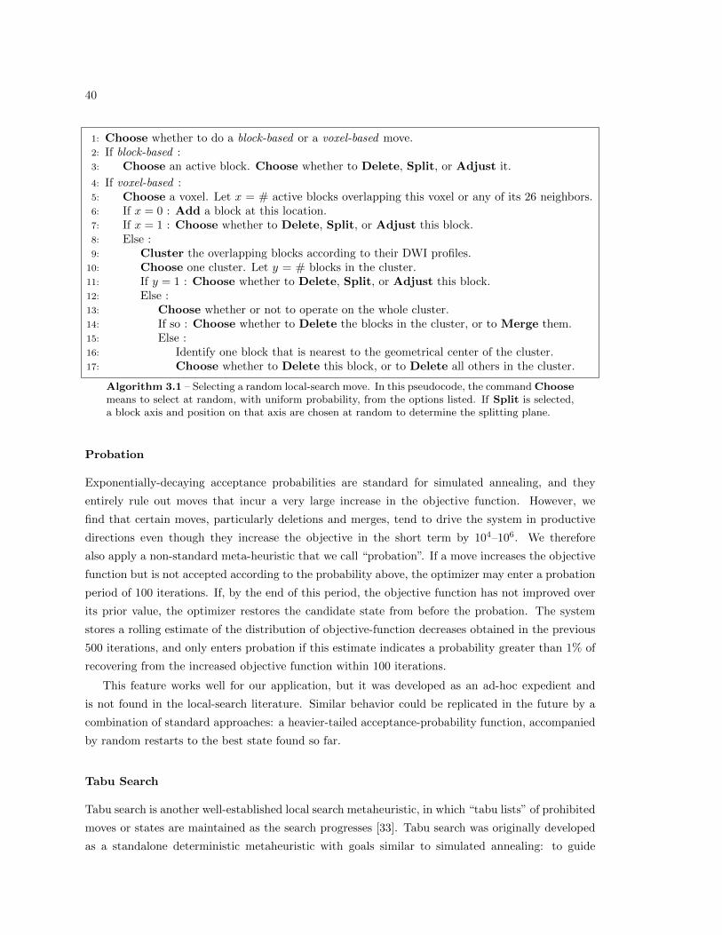
40

1: Choose whether to do a block-based or a voxel-based move.2: If block-based :3: Choose an active block. Choose whether to Delete, Split, or Adjust it.

4: If voxel-based :5: Choose a voxel. Let x = # active blocks overlapping this voxel or any of its 26 neighbors.6: If x = 0 : Add a block at this location.7: If x = 1 : Choose whether to Delete, Split, or Adjust this block.8: Else :9: Cluster the overlapping blocks according to their DWI profiles.

10: Choose one cluster. Let y = # blocks in the cluster.11: If y = 1 : Choose whether to Delete, Split, or Adjust this block.12: Else :13: Choose whether or not to operate on the whole cluster.14: If so : Choose whether to Delete the blocks in the cluster, or to Merge them.15: Else :16: Identify one block that is nearest to the geometrical center of the cluster.17: Choose whether to Delete this block, or to Delete all others in the cluster.

Algorithm 3.1 – Selecting a random local-search move. In this pseudocode, the command Choosemeans to select at random, with uniform probability, from the options listed. If Split is selected,a block axis and position on that axis are chosen at random to determine the splitting plane.

Probation

Exponentially-decaying acceptance probabilities are standard for simulated annealing, and they

entirely rule out moves that incur a very large increase in the objective function. However, we

find that certain moves, particularly deletions and merges, tend to drive the system in productive

directions even though they increase the objective in the short term by 104–106. We therefore

also apply a non-standard meta-heuristic that we call “probation”. If a move increases the objective

function but is not accepted according to the probability above, the optimizer may enter a probation

period of 100 iterations. If, by the end of this period, the objective function has not improved over

its prior value, the optimizer restores the candidate state from before the probation. The system

stores a rolling estimate of the distribution of objective-function decreases obtained in the previous

500 iterations, and only enters probation if this estimate indicates a probability greater than 1% of

recovering from the increased objective function within 100 iterations.

This feature works well for our application, but it was developed as an ad-hoc expedient and

is not found in the local-search literature. Similar behavior could be replicated in the future by a

combination of standard approaches: a heavier-tailed acceptance-probability function, accompanied

by random restarts to the best state found so far.

Tabu Search

Tabu search is another well-established local search metaheuristic, in which “tabu lists” of prohibited

moves or states are maintained as the search progresses [33]. Tabu search was originally developed

as a standalone deterministic metaheuristic with goals similar to simulated annealing: to guide

41

local search to explore a more diverse range of states by sometimes accepting moves that increase

the objective function in the short term. However, tabu search may also be applied in concert

with simulated annealing, despite the latter’s stochastic nature. We maintain tabu lists of recently

rejected moves, thereby preventing the simulated-annealing optimizer from repeatedly attempting

the same move after it fails once. The prohibition on rejected moves expires after 50 iterations.

This feature becomes important as the number of blocks decreases late in the optimization.

3.2.3 Initialization

In order to begin the search somewhat near a local optimum, we automatically generate the initial

model instance from pre-existing diffusion-based tissue-modeling techniques. We use Tournier, et al.’s

MRtrix software to perform multi-direction tractography [92, 93], and then sparsify the resulting

set of curves by culling redundant elements, using the method of Zhang, et al. [103]. The culling

method computes the dissimilarity between two curves as the mean of all pointwise minimum dis-

tances that are above a specific threshold. We use a threshold of 0.2 mm and cull the curves so that

the dissimilarity of each pair of curves is above 0.75 mm.

Given this decimated curve set, we construct a sort of “macaroni necklace” of small blocks along

each curve. We split each curve into segments 3 voxel-widths long, and align a single block (2 voxel-

widths wide in the orthogonal directions) along it. Each block has default appearance parameters

S0 = 300, M = 0.001 mm2/s, and F = 0.5, which are similar to the values found for white matter

imaged in clinical studies, but not identical to the values used in our computational phantoms.

3.2.4 Termination

The optimizer has two termination conditions: a convergence criterion, and an absolute limit on the

total number of iterations. If the system runs for 1500 iterations without improving the objective

function by more than 0.1, we consider this a signal of convergence and terminate. We also terminate

the system after 50,000 iterations total (approximately 13 hours, at one second per iteration on

average). In either case, at termination we return the model instance with the lowest objective value

found so far.

3.3 Evaluation

We evaluated the discrete–continuous fitting method on images of the eight subjects specified in

the previous chapter (§2.3), at two noise levels (σ ∈ {14.5, 29}) and two non-zero b-values (b ∈{1000 s/mm2, 3000 s/mm2}), again with 10 unweighted images and 64 diffusion-weighted images. Each

component of the test subjects had appearance values S0 = 290, M = 0.0007 mm2/s, and F = 0.7.

See Figure 2.1 for images of the test subjects.

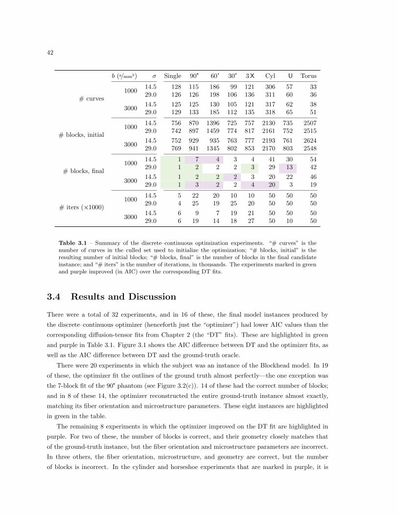
42

b (s/mm2) σ Single 90° 60° 30° 3X Cyl U Torus

# curves1000

14.5 128 115 186 99 121 306 57 3329.0 126 126 198 106 136 311 60 36

300014.5 125 125 130 105 121 317 62 3829.0 129 133 185 112 135 318 65 51

# blocks, initial1000

14.5 756 870 1396 725 757 2130 735 250729.0 742 897 1459 774 817 2161 752 2515

300014.5 752 929 935 763 777 2193 761 262429.0 769 941 1345 802 853 2170 803 2548

# blocks, final1000

14.5 1 7 4 3 4 41 30 5429.0 1 2 2 2 3 29 13 42

300014.5 1 2 2 2 3 20 22 4629.0 1 3 2 2 4 20 3 19

# iters (Ö1000)1000

14.5 5 22 20 10 10 50 50 5029.0 4 25 19 25 20 50 50 50

300014.5 6 9 7 19 21 50 50 5029.0 6 19 14 18 27 50 10 50

Table 3.1 – Summary of the discrete–continuous optimization experiments. “# curves” is thenumber of curves in the culled set used to initialize the optimization; “# blocks, initial” is theresulting number of initial blocks; “# blocks, final” is the number of blocks in the final candidateinstance; and “# iters” is the number of iterations, in thousands. The experiments marked in greenand purple improved (in AIC) over the corresponding DT fits.

3.4 Results and Discussion

There were a total of 32 experiments, and in 16 of these, the final model instances produced by

the discrete–continuous optimizer (henceforth just the “optimizer”) had lower AIC values than the

corresponding diffusion-tensor fits from Chapter 2 (the “DT” fits). These are highlighted in green

and purple in Table 3.1. Figure 3.1 shows the AIC difference between DT and the optimizer fits, as

well as the AIC difference between DT and the ground-truth oracle.

There were 20 experiments in which the subject was an instance of the Blockhead model. In 19

of these, the optimizer fit the outlines of the ground truth almost perfectly—the one exception was

the 7-block fit of the 90° phantom (see Figure 3.2(c)). 14 of these had the correct number of blocks;

and in 8 of these 14, the optimizer reconstructed the entire ground-truth instance almost exactly,

matching its fiber orientation and microstructure parameters. These eight instances are highlighted

in green in the table.

The remaining 8 experiments in which the optimizer improved on the DT fit are highlighted in

purple. For two of these, the number of blocks is correct, and their geometry closely matches that

of the ground-truth instance, but the fiber orientation and microstructure parameters are incorrect.

In three others, the fiber orientation, microstructure, and geometry are correct, but the number

of blocks is incorrect. In the cylinder and horseshoe experiments that are marked in purple, it is

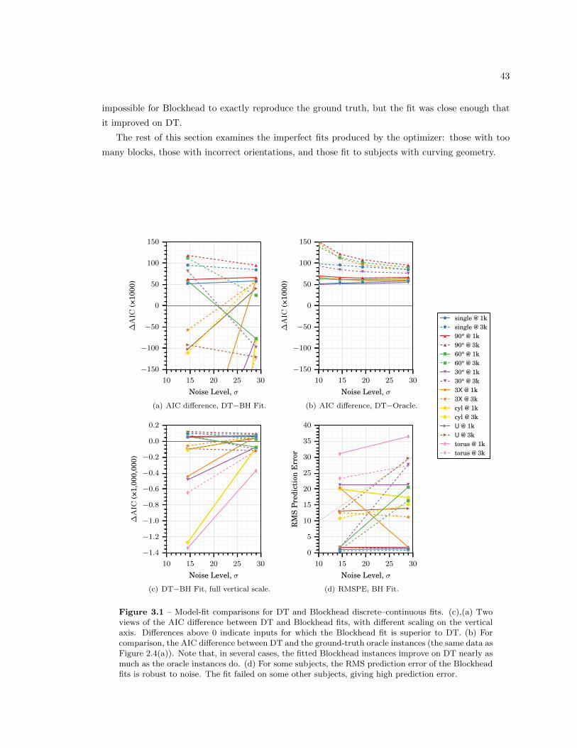
43

impossible for Blockhead to exactly reproduce the ground truth, but the fit was close enough that

it improved on DT.

The rest of this section examines the imperfect fits produced by the optimizer: those with too

many blocks, those with incorrect orientations, and those fit to subjects with curving geometry.

10 15 20 25 30

Noise Level, σ

−150

−100

−50

0

50

100

150

∆A

IC�(�×

�1�0�0�0

�)

single @ 1ksingle @ 3k�9�0�° @ 1k�9�0�° @ 3k�6�0�° @ 1k�6�0�° @ 3k�3�0�° @ 1k�3�0�° @ 3k3X @ 1k3X @ 3kcyl @ 1kcyl @ 3kU @ 1kU @ 3ktorus @ 1ktorus @ 3k

(a) AIC difference, DT−BH Fit.

10 15 20 25 30

Noise Level, σ

−150

−100

−50

0

50

100

150

∆A

IC�(�×

�1�0�0�0

�)

single @ 1ksingle @ 3k�9�0�° @ 1k�9�0�° @ 3k�6�0�° @ 1k�6�0�° @ 3k�3�0�° @ 1k�3�0�° @ 3k3X @ 1k3X @ 3k

(b) AIC difference, DT−Oracle.

0 5 10 15 20 25 30

Noise Level, σ

0

100

200

300

400

∆A

IC�(�×

�1�0�0�0

�)

single @ 1ksingle @ 3k�9�0�° @ 1k�9�0�° @ 3k�6�0�° @ 1k�6�0�° @ 3k�3�0�° @ 1k�3�0�° @ 3k3X @ 1k3X @ 3kcyl @ 1kcyl @ 3kU @ 1kU @ 3ktorus @ 1ktorus @ 3k

10 15 20 25 30

Noise Level, σ

−1.4

−1.2

−1.0

−0.8

−0.6

−0.4

−0.2

0.0

0.2

∆A

IC�(�×

�1�,�0�0

�0�,�0�0

�0�)

single @ 1ksingle @ 3k�9�0�° @ 1k�9�0�° @ 3k�6�0�° @ 1k�6�0�° @ 3k�3�0�° @ 1k�3�0�° @ 3k3X @ 1k3X @ 3kcyl @ 1kcyl @ 3kU @ 1kU @ 3ktorus @ 1ktorus @ 3k

(c) DT−BH Fit, full vertical scale.

10 15 20 25 30

Noise Level, σ

0

5

10

15

20

25

30

35

40

RM

SP

redi

ctio

nE

rror

single @ 1ksingle @ 3k�9�0�° @ 1k�9�0�° @ 3k�6�0�° @ 1k�6�0�° @ 3k�3�0�° @ 1k�3�0�° @ 3k3X @ 1k3X @ 3kcyl @ 1kcyl @ 3kU @ 1kU @ 3ktorus @ 1ktorus @ 3k

(d) RMSPE, BH Fit.

Figure 3.1 – Model-fit comparisons for DT and Blockhead discrete–continuous fits. (c),(a) Twoviews of the AIC difference between DT and Blockhead fits, with different scaling on the verticalaxis. Differences above 0 indicate inputs for which the Blockhead fit is superior to DT. (b) Forcomparison, the AIC difference between DT and the ground-truth oracle instances (the same data asFigure 2.4(a)). Note that, in several cases, the fitted Blockhead instances improve on DT nearly asmuch as the oracle instances do. (d) For some subjects, the RMS prediction error of the Blockheadfits is robust to noise. The fit failed on some other subjects, giving high prediction error.

44

3.4.1 Wrong Numbers of Blocks

Figure 3.2 shows three fits for which the −log(L) is low, and the fiber orientation in the fit model

instances corresponds to the ground truth, but the number of blocks is incorrect. We observe that,

as long as the outlines of the fit model instance match those of the ground truth, fairly significant

geometry errors can occur with negligible impact on AIC or −log(L).

Figure 3.2(a) (the 60° phantom, fit at b = 1000 s/mm2 and σ = 14.5) shows two examples of the

most common and benign geometry error: a structure that should be represented by one block,

which is instead split along the fiber axis into two blocks. Note that there are four blocks in this

figure: both of the true single-block structures are represented by two blocks. The faces of the split

blocks are precisely aligned, and the other faces of these blocks are aligned to the true outline of

the imaged subject. The appearance parameters in each block vary slightly, as they are overfitted

to the signals in the regions that they cover. The solver could have merged each of these two pairs,

incurring a temporary increase in AIC due to mismatching appearance. In this case, however, the

system had settled too strongly into the local minimum of these splits and did not accept any merge

moves. In 19 of the 20 experiments with Blockhead-based ground truth, the outlines of the ground-

truth instance were reconstructed exactly, just as they are here, though other mistakes decreased

the quality of the fit for some.

The one exception to the precise reconstruction of subject outlines is shown in Figure 3.2(c):

the 90° phantom, fit at b = 1000 s/mm2 and σ = 14.5. Here, seven blocks were used to reconstruct

a subject that in truth contained only two. The green and yellow blocks have very low S0 values,

so they barely contribute to the signal for this model instance; they are also the ones that fall

outside the outlines of the ground-truth instance. The orange, purple, and grey blocks have nearly

identical appearance parameters, and are aligned parallel to each other; they provide an example of

a slightly less common geometry error: splitting one block parallel to the fiber axis. This geometrical

characteristic appeared in a number of fits to the subjects with curving geometry. Since the Merge

move works only on two blocks at a time, merging either the purple or grey block with the orange

one would have incurred a temporary increase in AIC, as the merged block would overlap with the

remaining small slab, driving up the signal value in that region.

Figure 3.2(e) (90° phantom, at b = 3000 s/mm2, σ = 29.0) shows the least common geometry

error. Two blocks, a yellow one and an orange one, overlap almost exactly with each other. Their

microstructure parameters are very different, but the sum of their signal contributions matches the

ground truth. The current implementation of merging simply averages the microstructure param-

eters of the two input blocks, so a merger of the yellow and orange blocks in this case would have

higher −log(L).

3.4.2 Incorrect Fiber Orientation

Figure 3.3 shows three fits in which the geometry of the subject was recovered well, but the fiber

orientations of some blocks are incorrect. In Figure 3.3(a) (60° phantom, at b = 1000 s/mm2 and

45

(a) 60° @ b = 1000 s/mm2, σ = 14.5.

0 5 10 15 20 25 30

0

5

10

15

20

25

30

0

1

2

3

4

5

6

7

8

9

Mea

n−l

og(L

)pe

rob

serv

atio

n

(b) −log(L) image slice, z = 17.

(c) 90° @ b = 1000 s/mm2, σ = 14.5.

0 5 10 15 20 25 30

0

5

10

15

20

25

30

0

1

2

3

4

5

6

7

8

9

Mea

n−l

og(L

)pe

rob

serv

atio

n

(d) −log(L) image slice, z = 17.

(e) 90° @ b = 3000 s/mm2, σ = 29.0.

0 5 10 15 20 25 30

0

5

10

15

20

25

30

0

1

2

3

4

5

6

7

8

9M

ean−l

og(L

)pe

rob

serv

atio

n

(f) −log(L) image slice, z = 17.

Figure 3.2 – Blockhead discrete–continuous fits with the wrong number of blocks. All three of thesefits had lower AIC values than the corresponding DT fits. Note the light-blue −log(L) images; theDWIs of these instances almost exactly match the ground truth, and therefore have nearly optimal−log(L) values.

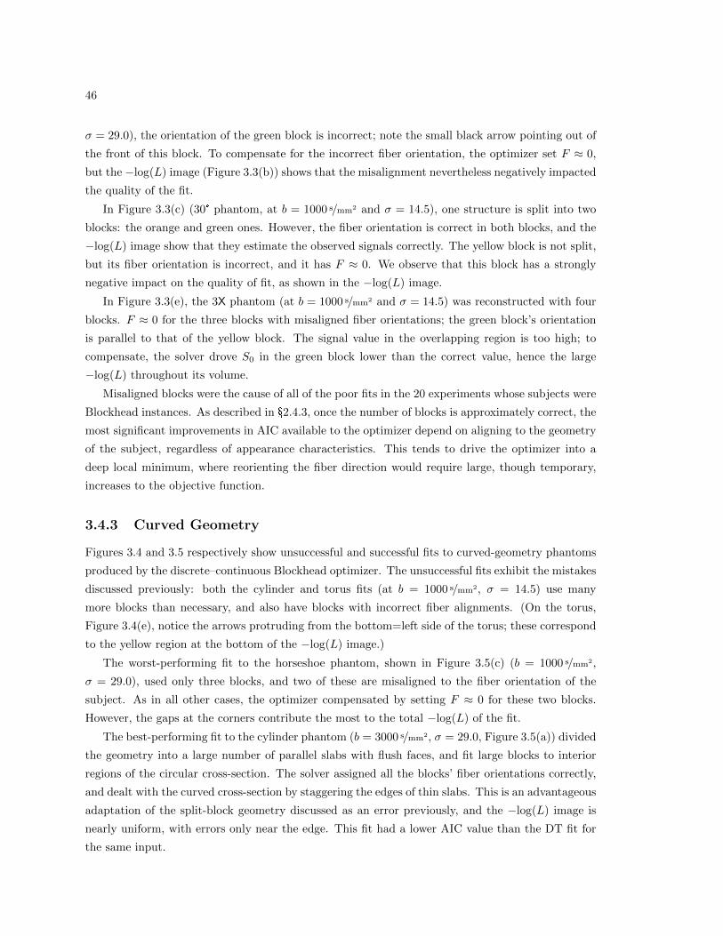
46

σ = 29.0), the orientation of the green block is incorrect; note the small black arrow pointing out of

the front of this block. To compensate for the incorrect fiber orientation, the optimizer set F ≈ 0,

but the −log(L) image (Figure 3.3(b)) shows that the misalignment nevertheless negatively impacted

the quality of the fit.

In Figure 3.3(c) (30° phantom, at b = 1000 s/mm2 and σ = 14.5), one structure is split into two

blocks: the orange and green ones. However, the fiber orientation is correct in both blocks, and the

−log(L) image show that they estimate the observed signals correctly. The yellow block is not split,

but its fiber orientation is incorrect, and it has F ≈ 0. We observe that this block has a strongly

negative impact on the quality of fit, as shown in the −log(L) image.

In Figure 3.3(e), the 3X phantom (at b = 1000 s/mm2 and σ = 14.5) was reconstructed with four

blocks. F ≈ 0 for the three blocks with misaligned fiber orientations; the green block’s orientation

is parallel to that of the yellow block. The signal value in the overlapping region is too high; to

compensate, the solver drove S0 in the green block lower than the correct value, hence the large

−log(L) throughout its volume.

Misaligned blocks were the cause of all of the poor fits in the 20 experiments whose subjects were

Blockhead instances. As described in §2.4.3, once the number of blocks is approximately correct, the

most significant improvements in AIC available to the optimizer depend on aligning to the geometry

of the subject, regardless of appearance characteristics. This tends to drive the optimizer into a

deep local minimum, where reorienting the fiber direction would require large, though temporary,

increases to the objective function.

3.4.3 Curved Geometry

Figures 3.4 and 3.5 respectively show unsuccessful and successful fits to curved-geometry phantoms

produced by the discrete–continuous Blockhead optimizer. The unsuccessful fits exhibit the mistakes

discussed previously: both the cylinder and torus fits (at b = 1000 s/mm2, σ = 14.5) use many

more blocks than necessary, and also have blocks with incorrect fiber alignments. (On the torus,

Figure 3.4(e), notice the arrows protruding from the bottom=left side of the torus; these correspond

to the yellow region at the bottom of the −log(L) image.)

The worst-performing fit to the horseshoe phantom, shown in Figure 3.5(c) (b = 1000 s/mm2,

σ = 29.0), used only three blocks, and two of these are misaligned to the fiber orientation of the

subject. As in all other cases, the optimizer compensated by setting F ≈ 0 for these two blocks.

However, the gaps at the corners contribute the most to the total −log(L) of the fit.

The best-performing fit to the cylinder phantom (b = 3000 s/mm2, σ = 29.0, Figure 3.5(a)) divided

the geometry into a large number of parallel slabs with flush faces, and fit large blocks to interior

regions of the circular cross-section. The solver assigned all the blocks’ fiber orientations correctly,

and dealt with the curved cross-section by staggering the edges of thin slabs. This is an advantageous

adaptation of the split-block geometry discussed as an error previously, and the −log(L) image is

nearly uniform, with errors only near the edge. This fit had a lower AIC value than the DT fit for

the same input.

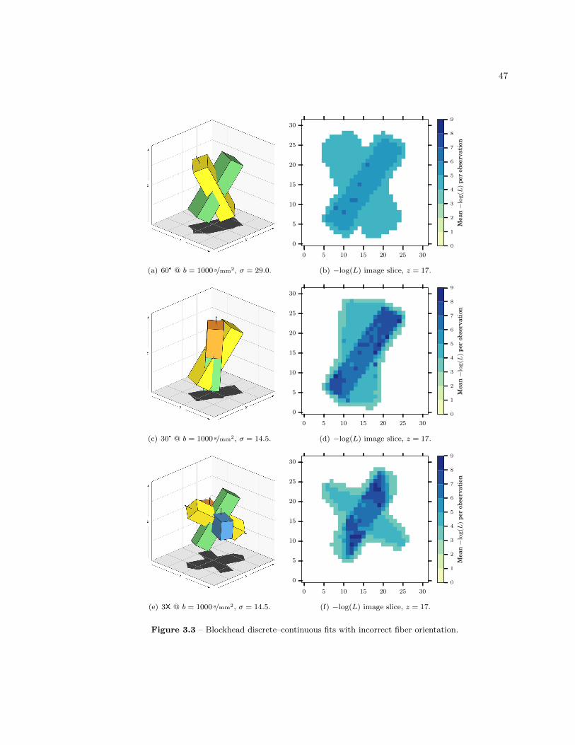
47

(a) 60° @ b = 1000 s/mm2, σ = 29.0.

0 5 10 15 20 25 30

0

5

10

15

20

25

30

0

1

2

3

4

5

6

7

8

9

Mea

n−l

og(L

)pe

rob

serv

atio

n

(b) −log(L) image slice, z = 17.

(c) 30° @ b = 1000 s/mm2, σ = 14.5.

0 5 10 15 20 25 30

0

5

10

15

20

25

30

0

1

2

3

4

5

6

7

8

9

Mea

n−l

og(L

)pe

rob

serv

atio

n

(d) −log(L) image slice, z = 17.

(e) 3X @ b = 1000 s/mm2, σ = 14.5.

0 5 10 15 20 25 30

0

5

10

15

20

25

30

0

1

2

3

4

5

6

7

8

9M

ean−l

og(L

)pe

rob

serv

atio

n

(f) −log(L) image slice, z = 17.

Figure 3.3 – Blockhead discrete–continuous fits with incorrect fiber orientation.

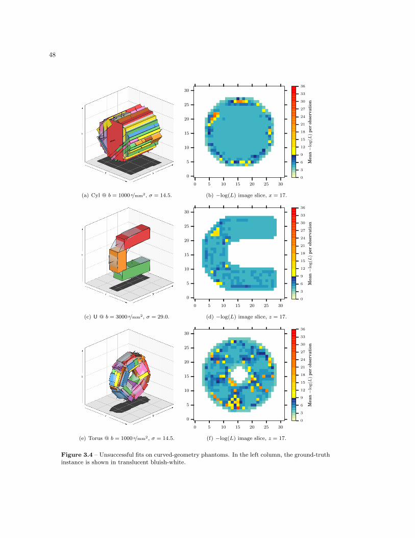
48

(a) Cyl @ b = 1000 s/mm2, σ = 14.5.

0 5 10 15 20 25 30

0

5

10

15

20

25

30

0

3

6

9

12

15

18

21

24

27

30

33

36

Mea

n−l

og(L

)pe

rob

serv

atio

n

(b) −log(L) image slice, x = 17.

(c) U @ b = 3000 s/mm2, σ = 29.0.

0 5 10 15 20 25 30

0

5

10

15

20

25

30

0

3

6

9

12

15

18

21

24

27

30

33

36

Mea

n−l

og(L

)pe

rob

serv

atio

n(d) −log(L) image slice, z = 17.

(e) Torus @ b = 1000 s/mm2, σ = 14.5.

0 5 10 15 20 25 30

0

5

10

15

20

25

30

0

3

6

9

12

15

18

21

24

27

30

33

36

Mea

n−l

og(L

)pe

rob

serv

atio

n

(f) −log(L) image slice, z = 17.

Figure 3.4 – Unsuccessful fits on curved-geometry phantoms. In the left column, the ground-truthinstance is shown in translucent bluish-white.

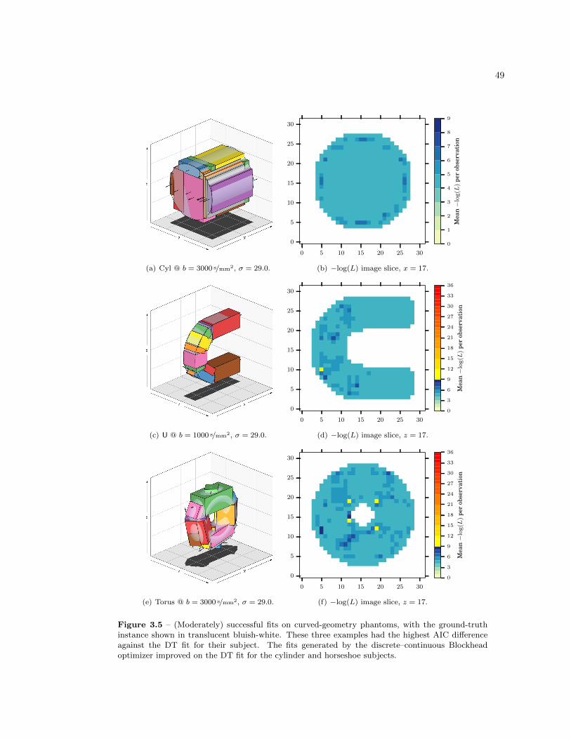
49

(a) Cyl @ b = 3000 s/mm2, σ = 29.0.

0 5 10 15 20 25 30

0

5

10

15

20

25

30

0

1

2

3

4

5

6

7

8

9

Mea

n−l

og(L

)pe

rob

serv

atio

n

(b) −log(L) image slice, x = 17.

(c) U @ b = 1000 s/mm2, σ = 29.0.

0 5 10 15 20 25 30

0

5

10

15

20

25

30

0

3

6

9

12

15

18

21

24

27

30

33

36

Mea

n−l

og(L

)pe

rob

serv

atio

n

(d) −log(L) image slice, z = 17.

(e) Torus @ b = 3000 s/mm2, σ = 29.0.

0 5 10 15 20 25 30

0

5

10

15

20

25

30

0

3

6

9

12

15

18

21

24

27

30

33

36

Mea

n−l

og(L

)pe

rob

serv

atio

n

(f) −log(L) image slice, z = 17.

Figure 3.5 – (Moderately) successful fits on curved-geometry phantoms, with the ground-truthinstance shown in translucent bluish-white. These three examples had the highest AIC differenceagainst the DT fit for their subject. The fits generated by the discrete–continuous Blockheadoptimizer improved on the DT fit for the cylinder and horseshoe subjects.

50

The best-fit horseshoe example (b = 1000 s/mm2, σ = 29.0, Figure 3.5(c)) also improved on DT’s

AIC value. Here the fiber orientations are again correct throughout. The optimizer adapted in two

ways to the curving main axis. On the top part of the curve, it segmented the subject’s geometry

orthogonal to its axis, and represented each segment with one block. On the bottom part of the

curve, it found a larger, keystone-shaped segment, but represented it with two blocks (the red and

blue ones) arranged in parallel circumferential layers.

The best-fit torus example (b = 3000 s/mm2, σ = 29.0, Figure 3.5(e)) did not improve over DT, and

though the −log(L) image appears nearly uniform, there are scattered high-error voxels throughout

the volume. In this case the solver again used fewer blocks than are probably necessary to avoid

leaving large gaps or going outside the boundary of the ground-truth subject.

3.5 Conclusions

The mixed discrete–continuous local-search optimizer described in this chapter successfully recov-

ered the ground-truth model instances in 8 experiments. In many other experiments, it made a

single consistent error of misaligning the fiber orientation in a block, due to the stronger influence

that geometry exerts over the fitting process. This observation suggests a future development: an

additional discrete “Fiber Swap” move, which would exchange the order of the axes of a block, mak-

ing the fibers point in a different direction. This move would allow the optimizer to easily correct

fiber-orientation mistakes, even late in the optimization process.

The optimizer also fit curving geometry relatively well, finding solutions in 2 out of 12 experiments

that had quality (in the sense of AIC value) superior to that of the corresponding diffusion-tensor fits.

It adapted to the restrictive, hard-angled geometry of the Blockhead model in three ways: staggering

parallel blocks to give a “stairstepped” outline, arranging sequences of short blocks at small angles

to each other along curving-fiber regions, and splitting curving-fiber regions parallel to the fiber

axis, placing shorter blocks on the inside of the curve and longer blocks on the outside. Minor

modifications to the geometry model could enable the solver to fit these instances even better. Some

possibilities include allowing the primary ends of each block (the faces orthogonal to the primary

axis) to tilt, allowing the cross-section to be a superellipse, allowing the cross-sectional area to vary

along the length of the block, and composing block shapes with constructive solid geometry.

The partial success of the optimizer, despite the restrictive geometry of the model and the in-

complete tuning of the search metaheuristics, demonstrates that the AIC is an appropriate objective

function for this problem. Furthermore, this chapter describes a novel adaptation of the contin-

uous aspects of the Blockhead modeling problem: the concepts of an “adjustment iteration” and

an expanding “known universe” of solution components. This approach allows standard tools of

combinatorial optimization, such as simulated annealing, to be applied to a modeling problem that

has both discrete and continuous characteristics.

Chapter 4

Physical-Phantom Experiments

4.1 Introduction

The previous two chapters described experiments aimed at fitting a Blockhead model instance to

synthetic images of computational phantoms with highly regular geometry. In this chapter we briefly

examine the behavior of the system when attempting to fit to real diffusion-weighted MR images

of a physical phantom. This demonstrates the modeling system’s behavior when confronted with

a low-resolution, low-SNR image of a structure with varied morphology, for which we nevertheless

know the ground-truth structure.

4.2 Methods and Evaluation

The “Fiber Cup” phantom was developed as a tractography benchmark by Fillard et al. in 2009 [31].

This physical phantom consists of a 14 cm-diameter disk-shaped polyurethane housing, holding thou-

sands of impermeable acrylic fibers, each 20µm thick. The structure has five fiber bundles that

exhibit bending, crossing, kissing, and fanning geometries, arranged in a configuration that roughly

mimics a mid-coronal section through the human brain.

Fillard et al. scanned the phantom and made diffusion-weighted images publicly available in

several datasets, differing by non-zero b-value and voxel size. Each dataset consists of 130 images in

total: two repetitions of an acquisition with one unweighted image and 64 images diffusion-weighted

in distinct gradient directions. We used two datasets, with b ∈ {1500 s/mm2, 2000 s/mm2}, 3 mm

isotropic voxels, and 64Ö64Ö3 voxels in the imaging volume. For simplicity, in this chapter we refer

to these as the “low-b” and “high-b” datasets, respectively. The estimated noise level in the images

was 8.4. Table 4.1 shows various measures of the two datasets, and Figure 4.1 shows example DWIs.

We used the discrete–continuous optimization technique described in Chapter 3 to fit Blockhead

model instances to the two datasets, with the Akaike information criterion as the objective function.

To initialize the search, we first computed multi-direction, CSD-based tractography curves with

MRtrix [92, 93], sparsified them by the method of Zhang, et al. [103], broke the curves into 9 mm

segments, and finally constructed one block for each segment. Figure 4.2 shows the initial model

instance for the low-b dataset.

51

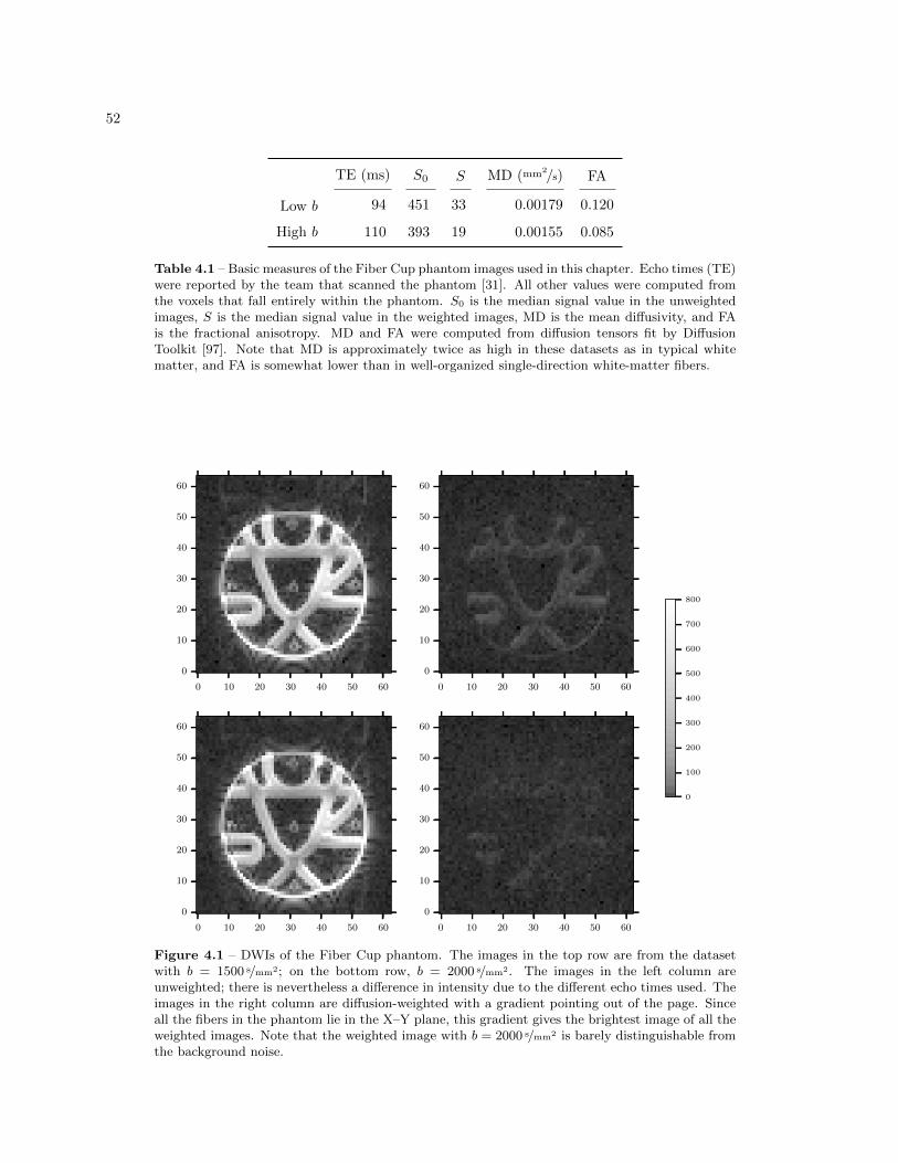
52

TE (ms) S0 S MD (mm2/s) FA

Low b 94 451 33 0.00179 0.120

High b 110 393 19 0.00155 0.085

Table 4.1 – Basic measures of the Fiber Cup phantom images used in this chapter. Echo times (TE)were reported by the team that scanned the phantom [31]. All other values were computed fromthe voxels that fall entirely within the phantom. S0 is the median signal value in the unweightedimages, S is the median signal value in the weighted images, MD is the mean diffusivity, and FAis the fractional anisotropy. MD and FA were computed from diffusion tensors fit by DiffusionToolkit [97]. Note that MD is approximately twice as high in these datasets as in typical whitematter, and FA is somewhat lower than in well-organized single-direction white-matter fibers.

0 10 20 30 40 50 60

0

10

20

30

40

50

60

0

100

200

300

400

500

600

700

800

0 10 20 30 40 50 60

0

10

20

30

40

50

60

0

100

200

300

400

500

600

700

800

0 10 20 30 40 50 60

0

10

20

30

40

50

60

0

100

200

300

400

500

600

700

800

0 10 20 30 40 50 60

0

10

20

30

40

50

60

0

100

200

300

400

500

600

700

800

0 10 20 30 40 50 60

0

10

20

30

40

50

60

0

100

200

300

400

500

600

700

800

Figure 4.1 – DWIs of the Fiber Cup phantom. The images in the top row are from the datasetwith b = 1500 s/mm2; on the bottom row, b = 2000 s/mm2. The images in the left column areunweighted; there is nevertheless a difference in intensity due to the different echo times used. Theimages in the right column are diffusion-weighted with a gradient pointing out of the page. Sinceall the fibers in the phantom lie in the X–Y plane, this gradient gives the brightest image of all theweighted images. Note that the weighted image with b = 2000 s/mm2 is barely distinguishable fromthe background noise.

53

Figure 4.2 – InitialBlockhead model instancefor the low-b Fiber Cupdataset. There are a totalof 907 blocks.

As a baseline for comparison, we also used Diffusion Toolkit to compute diffusion-tensor model

fits for the two datasets. We computed a mask with 2253 voxels containing signals from the phantom

fibers, which we used both for comparison between model fits and also as the foreground mask for

the discrete–continuous optimization.

We modified the input data slightly, padding the image volumes on both sides in the Z direction

with a layer of pure Rician noise 9 mm (3 voxels) thick. Without this modification, candidate

Blockhead instances with components that erroneously extended out of the plane of the subject

would have incurred no penalty in the objective function. All of these added voxels were masked

out, so they did not factor into the AIC measurements of the DT model.

4.3 Results and Discussion

The optimization process had limited success modeling the curving and intersecting geometry of

the Fiber Cup phantom. For both datasets, the diffusion-tensor model had a far superior fit, in

terms of Akaike information criterion: the AIC was higher for the Blockhead fits by 6.5× 106 in the

low-b dataset, and by 3.1 × 106 in the high-b dataset. This is a discrepancy 2–4 times as large as

that between DT and the most poorly-scoring automatic Blockhead fits in Chapter 3 (those for the

Cylinder and Torus datasets; c.f. Figure 3.1).

Figure 4.3 shows the final Blockhead instances produced for the two datasets. Two modest

successes of the fitting method may be observed:

� There are no blocks that go significantly out of the plane of the phantom. As observed

previously, the 3-D “silhouette” of the subject forms the strongest signal for the solver, leading

it to construct blocks that match flat faces of the subject when they are present.

� The final Blockhead instance generally succeeded in modeling isolated straight segments of

tracts, including the near-vertical one on the left side of the phantom, the lowest of the three

branches on the right side, and also (in the low-b dataset) several others around the 90° crossing

at the bottom. The fit instance uses only one or two blocks to model each of these structures,

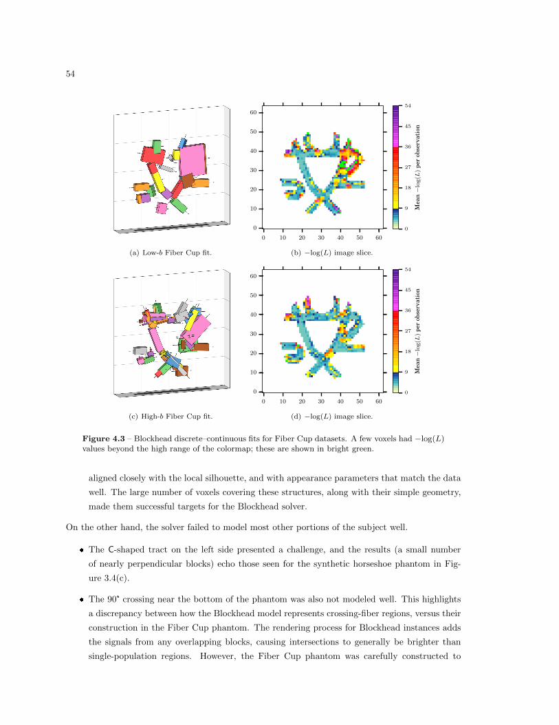
54

(a) Low-b Fiber Cup fit.

0 10 20 30 40 50 60

0

10

20

30

40

50

60

0

9

18

27

36

45

54

Mea

n−l

og(L

)pe

rob

serv

atio

n

(b) −log(L) image slice.

(c) High-b Fiber Cup fit.

0 10 20 30 40 50 60

0

10

20

30

40

50

60

0

9

18

27

36

45

54

Mea

n−l

og(L

)pe

rob

serv

atio

n(d) −log(L) image slice.

Figure 4.3 – Blockhead discrete–continuous fits for Fiber Cup datasets. A few voxels had −log(L)values beyond the high range of the colormap; these are shown in bright green.

aligned closely with the local silhouette, and with appearance parameters that match the data

well. The large number of voxels covering these structures, along with their simple geometry,

made them successful targets for the Blockhead solver.

On the other hand, the solver failed to model most other portions of the subject well.

� The C-shaped tract on the left side presented a challenge, and the results (a small number

of nearly perpendicular blocks) echo those seen for the synthetic horseshoe phantom in Fig-

ure 3.4(c).

� The 90° crossing near the bottom of the phantom was also not modeled well. This highlights

a discrepancy between how the Blockhead model represents crossing-fiber regions, versus their

construction in the Fiber Cup phantom. The rendering process for Blockhead instances adds

the signals from any overlapping blocks, causing intersections to generally be brighter than

single-population regions. However, the Fiber Cup phantom was carefully constructed to

55

ensure that the cross-sectional density of the acrylic fibers remained constant (at about 1900

fibers per mm2) throughout, including crossing regions. This required removing half or a third

of the fibers from each crossing region. While axons in real white-matter tissue terminate only

at the ends of tracts, this was the only practical way to handle crossing-fiber regions with

incompressible acrylic fibers. In Figure 4.1, it can be observed that the unweighted signal

in the 90° crossing region is slightly lower than in the surrounding regions, contrary to the

rendered result for two crossing Blockhead blocks.

� For both datasets, the solver used one large block to cover both of the upper branches on

the right side. In the low-b dataset, this one block extended even further upward, covering

the top of the steepest tract as well as the rightmost portion of the horizontal tract, and

the intersection of these two. The −log(L) images show that this was not a successful fit,

particularly in the low-b case.

� In other regions, the solver attempted either to model large portions of subtly varying geometry

with a small number of blocks, or failed to combine small “shard” blocks into larger ones. This

is again consistent with the failure modes observed in Chapter 3 for curving geometry.

4.4 Conclusions

The results for the Fiber Cup phantom highlight many of the same shortcomings of the Blockhead

model remarked upon in §3.5. Only structures with a rectilinear shape can be modeled well by a

Blockhead model instance; in all other cases, the solver adapts in a small number of ways to attempt

to represent more complicated structures. However, with high noise and large voxels relative to the

size of the structures of interest, the optimization method tends to obscure fine detail. This failure

case is an additional challenge on the way to modeling real brain structures with a Blockhead-like

model: many important white-matter tracts in the human brain are just millimeters wide.

56

Chapter 5

Conclusions and Open Problems

5.1 Optimization

Modeling coherent, multi-voxel structures with the Blockhead model is an example of an optimization

problem that has both discrete and continuous properties, and in which the number of model degrees

of freedom must also be optimized. The experiments in Chapters 2 and 3 demonstrate that the

Akaike information criterion (AIC) is an appropriate objective function for such a task. Minimizing

AIC leads to model instances that not only balance accuracy and parsimony, but also have low error

versus the unknown ground truth. The AIC is also a compelling objective function because it requires

no subjective choices with regard to weighting parameters, energy functions, or regularization terms,

and because it is an appropriate statistical tool for comparing the quality of fit for instances of diverse

models, including those that are not candidates in the optimization process.

The Blockhead optimization method demonstrates one approach to unifying the tools of discrete

and continuous optimization in a way that is amenable to standard combinatorial search metaheuris-

tics. The notable characteristics of this approach include:

� We formalize the search problem as the selection of a subset of an infinite universe of immutable

discrete components. Any given subset corresponds to a unique model instance.

� Rather than attempt to represent the entire universe of the search space, as the search proceeds,

we represent only the “known universe”: the union of all candidate subsets so far.

� The search neighborhood around a candidate instance includes not only discrete moves, but

single steps of various adjustments to continuous parameters as well.

� Continuous moves do not modify existing elements of the known universe. Instead, the outcome

of a continuous move is that a new element is appended to the known universe.

5.2 Tissue Modeling

Neuroscientists and other researchers interested in brain white-matter structure typically think of

this tissue in terms of its anatomical components, the fascicles. When relying on diffusion MRI to

57

58

investigate the white matter non-invasively, these researchers therefore commonly have the task of

identifying one or more fascicles of interest in their data, in order to then compare them between

subjects, longitudinally over time, or between hemispheres of the same subject. Quantitative com-

parisons are often made between derived properties of the representations of these fascicles, including

fiber length, fascicle volume, and indicators of tissue integrity. Various researchers have attempted

to develop algorithms for the automatic segmentation of fascicles of interest [65, 58, 37], but in

practice, selection is almost always performed manually from tractography data, based on expert

anatomical knowledge [67]. This causes a significant labor burden in large studies, and also impacts

the stability and repeatability of results.

The Blockhead model presented in this dissertation is a rudimentary implementation of a general

proposed strategy for modeling the white matter, with the goal of supporting the automatic seg-

mentation and quantification of structures of interest. The two fundamental characteristics of this

strategy are that each model instance is composed of several distinct geometrical components, and

that each component contains a smooth function defined over its interior volume that determines

its microstructure properties (and thereby its appearance in synthetic DWIs). Ideally, the model

instance would support easy selection of structures of interest either by having each component

correspond to an individual fascicle in the true anatomy of the subject, or by storing associations

between components to indicate that they represent different portions of the same fascicle.

In the current Blockhead model, the geometrical components are rectangular cuboids, with no

representation of shared membership in the same fascicle. The microstructure properties represented

in each cuboid are the fractional anisotropy and mean diffusivity of a prolate diffusion tensor, along

with the unweighted diffusion signal S0; these are constant throughout the cuboid’s volume. Despite

the restrictive nature of this model, it exhibits some advantages over other models described in

Chapter 1, which serve as evidence that a more sophisticated model of this sort could have further

advantages.

In particular, the fitted Blockhead instances shown in Chapter 3 have a relatively small number

of components, each with a significant area when displayed on a two-dimensional screen. From

the perspective of human-computer interaction, this presents an easier selection task than manual

selection of tractography curves. Furthermore, the volume of each block is well-defined, in contrast

to a set of one-dimensional tractography curves in space. Finally, each set of microstructure param-

eters is fit against a large number of signal samples, leading to the noise-invariant RMSPE among

successful fits reported in Figure 3.1(d).

5.3 Open Questions

In addition to its mixture of discrete and continuous properties, another challenging aspect of the

Blockhead modeling problem is that the objective function is relatively expensive to compute, since

each function evaluation involves rendering synthetic DWIs. There is a diverse literature on op-

timization with expensive objective functions [22, 50, 102]. Combining these techniques with the

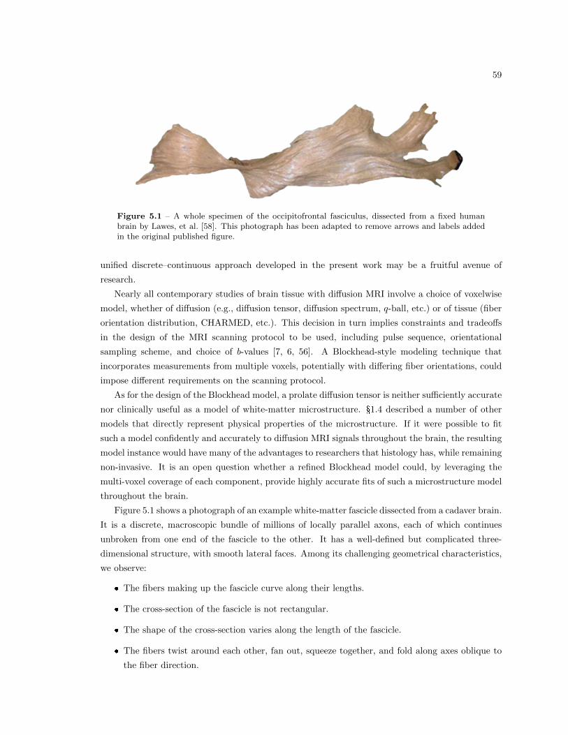
59

Figure 5.1 – A whole specimen of the occipitofrontal fasciculus, dissected from a fixed humanbrain by Lawes, et al. [58]. This photograph has been adapted to remove arrows and labels addedin the original published figure.

unified discrete–continuous approach developed in the present work may be a fruitful avenue of

research.

Nearly all contemporary studies of brain tissue with diffusion MRI involve a choice of voxelwise

model, whether of diffusion (e.g., diffusion tensor, diffusion spectrum, q-ball, etc.) or of tissue (fiber

orientation distribution, CHARMED, etc.). This decision in turn implies constraints and tradeoffs

in the design of the MRI scanning protocol to be used, including pulse sequence, orientational

sampling scheme, and choice of b-values [7, 6, 56]. A Blockhead-style modeling technique that

incorporates measurements from multiple voxels, potentially with differing fiber orientations, could

impose different requirements on the scanning protocol.

As for the design of the Blockhead model, a prolate diffusion tensor is neither sufficiently accurate

nor clinically useful as a model of white-matter microstructure. §1.4 described a number of other

models that directly represent physical properties of the microstructure. If it were possible to fit

such a model confidently and accurately to diffusion MRI signals throughout the brain, the resulting

model instance would have many of the advantages to researchers that histology has, while remaining

non-invasive. It is an open question whether a refined Blockhead model could, by leveraging the

multi-voxel coverage of each component, provide highly accurate fits of such a microstructure model

throughout the brain.

Figure 5.1 shows a photograph of an example white-matter fascicle dissected from a cadaver brain.

It is a discrete, macroscopic bundle of millions of locally parallel axons, each of which continues

unbroken from one end of the fascicle to the other. It has a well-defined but complicated three-

dimensional structure, with smooth lateral faces. Among its challenging geometrical characteristics,

we observe:

� The fibers making up the fascicle curve along their lengths.

� The cross-section of the fascicle is not rectangular.

� The shape of the cross-section varies along the length of the fascicle.

� The fibers twist around each other, fan out, squeeze together, and fold along axes oblique to

the fiber direction.

60

� The structure as a whole branches into three fiber bundles near the right end.

� The ends of the fascicle appear, at this length scale, not to be orthogonal to the fibers.

Accounting for all these natural geometrical properties in a Blockhead-style model, while still

maintaining a representation whose optimization is computationally tractable, is an open problem.

Possible avenues of investigation include generalizing the shape that each component can take on,

and possibly also associating neighboring components as being part of the same fascicle.

A more sophisticated representation of macrostructure geometry would also interact numerically

with the microstructure model. Consider a surface in space that intersects the fascicle and is locally

orthogonal to every axon. Call the intersection of this surface with the volume of the fascicle a “cross-

section”. (This is one possible generalization to the idea of a cross-section in a fibrous structure with

such complicated geometry.) Since each axon continues unbroken from one end of the fascicle to the

other, the number of axons passing through any two cross-sections must be equal. If the area of two

cross-sections is different, however, this implies that either the diameters or the packing density of

the axons within the cross-sections must differ. Incorporating this interaction between parameters

into an optimization system for a refined Blockhead model is an additional open problem.

Both the promising results demonstrated for the simplistic Blockhead implementation, and also

the variety of incremental changes that could improve the model, suggest the potential for later

iterations of this work to contribute meaningfully to research in numerical optimization as well as

white-matter tissue modeling.

Bibliography

[1] Milton Abramowitz and Irene A. Stegun. Handbook of Mathematical Functions. National

Bureau of Standards, 10th edition, 1972.

[2] Hirotugu Akaike. A New Look at the Statistical Model Identification. IEEE Transactions on

Automatic Control, 19(6):716—-723, 1974.

[3] Andrew L. Alexander, Khader M. Hasan, Mariana Lazar, Jay S. Tsuruda, and Dennis L.

Parker. Analysis of Partial Volume Effects in Diffusion-Tensor MRI. Magnetic Resonance in

Medicine, 45(5):770–780, 2001.

[4] Daniel C. Alexander. An Introduction to Computational Diffusion MRI: The Diffusion Tensor

and Beyond. In Joachim Weickert and Hans Hagen, editors, Visualization and Processing of

Tensor Fields, pages 83–106. Springer, Berlin, 2005.

[5] Daniel C. Alexander. Multiple-Fiber Reconstruction Algorithms for Diffusion MRI. Annals of

the New York Academy of Sciences, 1064:113–33, December 2005.

[6] Daniel C. Alexander. A General Framework for Experiment Design in Diffusion MRI and

Its Application in Measuring Direct Tissue-Microstructure Features. Magnetic Resonance in

Medicine, 60(2):439–448, 2008.

[7] Daniel C. Alexander and Gareth J. Barker. Optimal Imaging Parameters for Fiber-Orientation

Estimation in Diffusion MRI. NeuroImage, 27(2):357–67, August 2005.

[8] D. E. Amos. A Portable Package for Bessel Functions of a Complex Argument and Nonnegative

Order. ACM Transactions on Mathematical Software, 12(3):265–273, 1986.

[9] Yaniv Assaf and Peter J. Basser. Composite Hindered and Restricted Model of Diffusion

(CHARMED) MR Imaging of the Human Brain. NeuroImage, 27:48–58, 2005.

[10] Yaniv Assaf, Tamar Blumenfeld-Katzir, Yossi Yovel, and Peter J. Basser. AxCaliber: A

Method for Measuring Axon Diameter Distribution from Diffusion MRI. Magnetic Resonance

in Medicine, 59(6):1347–54, June 2008.

[11] Yaniv Assaf, Raisa Z. Freidlin, Gustavo K. Rohde, and Peter J. Basser. New Modeling and

Experimental Framework to Characterize Hindered and Restricted Water Diffusion in Brain

White Matter. Magnetic Resonance in Medicine, 52(5):965–978, 2004.

61

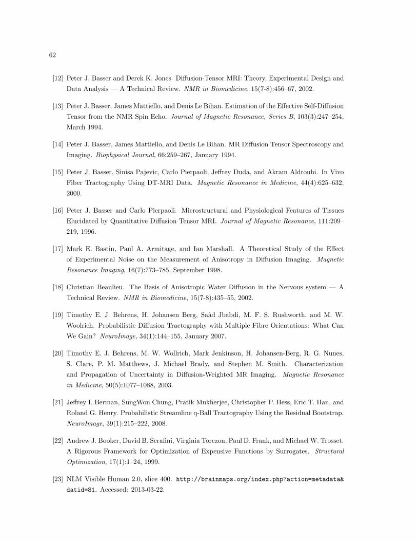
62

[12] Peter J. Basser and Derek K. Jones. Diffusion-Tensor MRI: Theory, Experimental Design and

Data Analysis — A Technical Review. NMR in Biomedicine, 15(7-8):456–67, 2002.

[13] Peter J. Basser, James Mattiello, and Denis Le Bihan. Estimation of the Effective Self-Diffusion

Tensor from the NMR Spin Echo. Journal of Magnetic Resonance, Series B, 103(3):247–254,

March 1994.

[14] Peter J. Basser, James Mattiello, and Denis Le Bihan. MR Diffusion Tensor Spectroscopy and

Imaging. Biophysical Journal, 66:259–267, January 1994.

[15] Peter J. Basser, Sinisa Pajevic, Carlo Pierpaoli, Jeffrey Duda, and Akram Aldroubi. In Vivo

Fiber Tractography Using DT-MRI Data. Magnetic Resonance in Medicine, 44(4):625–632,

2000.

[16] Peter J. Basser and Carlo Pierpaoli. Microstructural and Physiological Features of Tissues

Elucidated by Quantitative Diffusion Tensor MRI. Journal of Magnetic Resonance, 111:209–

219, 1996.

[17] Mark E. Bastin, Paul A. Armitage, and Ian Marshall. A Theoretical Study of the Effect

of Experimental Noise on the Measurement of Anisotropy in Diffusion Imaging. Magnetic

Resonance Imaging, 16(7):773–785, September 1998.

[18] Christian Beaulieu. The Basis of Anisotropic Water Diffusion in the Nervous system — A

Technical Review. NMR in Biomedicine, 15(7-8):435–55, 2002.

[19] Timothy E. J. Behrens, H. Johansen Berg, Saad Jbabdi, M. F. S. Rushworth, and M. W.

Woolrich. Probabilistic Diffusion Tractography with Multiple Fibre Orientations: What Can

We Gain? NeuroImage, 34(1):144–155, January 2007.

[20] Timothy E. J. Behrens, M. W. Wollrich, Mark Jenkinson, H. Johansen-Berg, R. G. Nunes,

S. Clare, P. M. Matthews, J. Michael Brady, and Stephen M. Smith. Characterization

and Propagation of Uncertainty in Diffusion-Weighted MR Imaging. Magnetic Resonance

in Medicine, 50(5):1077–1088, 2003.

[21] Jeffrey I. Berman, SungWon Chung, Pratik Mukherjee, Christopher P. Hess, Eric T. Han, and

Roland G. Henry. Probabilistic Streamline q-Ball Tractography Using the Residual Bootstrap.

NeuroImage, 39(1):215–222, 2008.

[22] Andrew J. Booker, David B. Serafini, Virginia Torczon, Paul D. Frank, and Michael W. Trosset.

A Rigorous Framework for Optimization of Expensive Functions by Surrogates. Structural

Optimization, 17(1):1–24, 1999.

[23] NLM Visible Human 2.0, slice 400. http://brainmaps.org/index.php?action=metadata&

datid=81. Accessed: 2013-03-22.

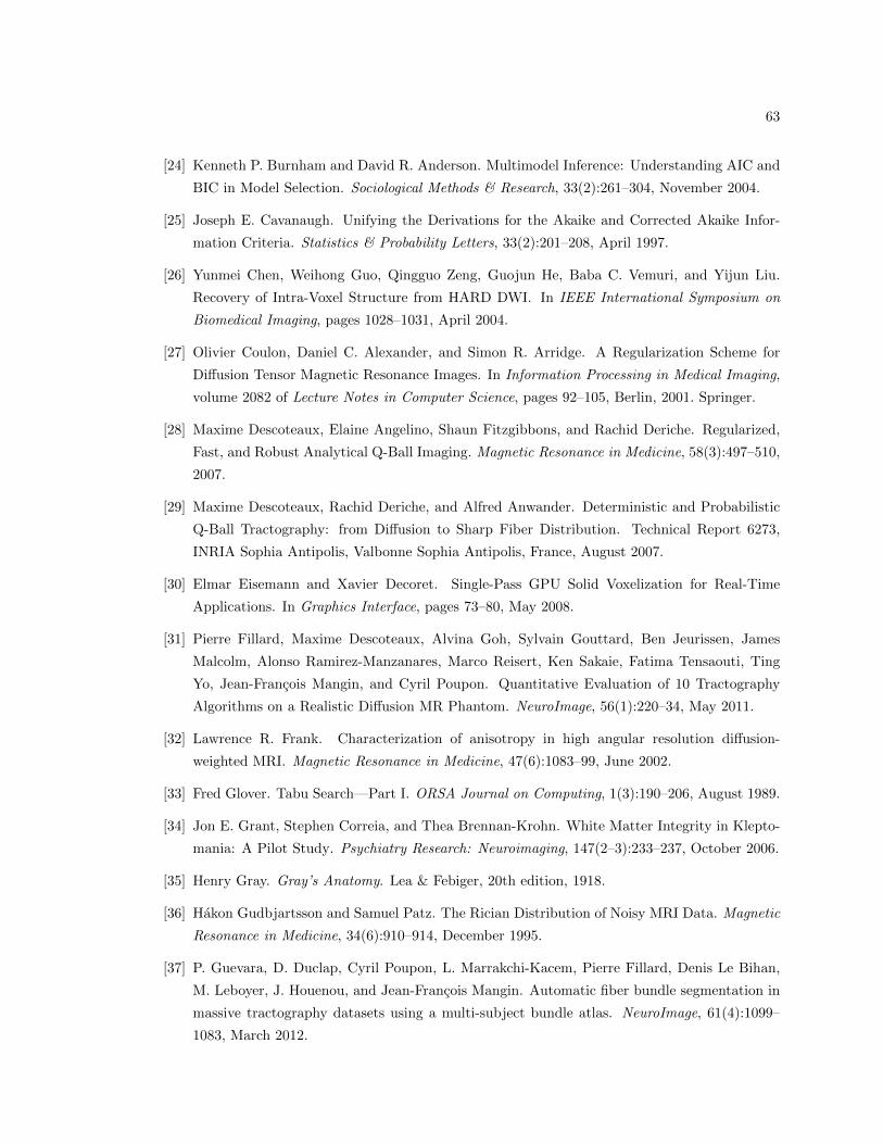
63

[24] Kenneth P. Burnham and David R. Anderson. Multimodel Inference: Understanding AIC and

BIC in Model Selection. Sociological Methods & Research, 33(2):261–304, November 2004.

[25] Joseph E. Cavanaugh. Unifying the Derivations for the Akaike and Corrected Akaike Infor-

mation Criteria. Statistics & Probability Letters, 33(2):201–208, April 1997.

[26] Yunmei Chen, Weihong Guo, Qingguo Zeng, Guojun He, Baba C. Vemuri, and Yijun Liu.

Recovery of Intra-Voxel Structure from HARD DWI. In IEEE International Symposium on

Biomedical Imaging, pages 1028–1031, April 2004.

[27] Olivier Coulon, Daniel C. Alexander, and Simon R. Arridge. A Regularization Scheme for

Diffusion Tensor Magnetic Resonance Images. In Information Processing in Medical Imaging,

volume 2082 of Lecture Notes in Computer Science, pages 92–105, Berlin, 2001. Springer.

[28] Maxime Descoteaux, Elaine Angelino, Shaun Fitzgibbons, and Rachid Deriche. Regularized,

Fast, and Robust Analytical Q-Ball Imaging. Magnetic Resonance in Medicine, 58(3):497–510,

2007.

[29] Maxime Descoteaux, Rachid Deriche, and Alfred Anwander. Deterministic and Probabilistic

Q-Ball Tractography: from Diffusion to Sharp Fiber Distribution. Technical Report 6273,

INRIA Sophia Antipolis, Valbonne Sophia Antipolis, France, August 2007.

[30] Elmar Eisemann and Xavier Decoret. Single-Pass GPU Solid Voxelization for Real-Time

Applications. In Graphics Interface, pages 73–80, May 2008.

[31] Pierre Fillard, Maxime Descoteaux, Alvina Goh, Sylvain Gouttard, Ben Jeurissen, James

Malcolm, Alonso Ramirez-Manzanares, Marco Reisert, Ken Sakaie, Fatima Tensaouti, Ting

Yo, Jean-Francois Mangin, and Cyril Poupon. Quantitative Evaluation of 10 Tractography

Algorithms on a Realistic Diffusion MR Phantom. NeuroImage, 56(1):220–34, May 2011.

[32] Lawrence R. Frank. Characterization of anisotropy in high angular resolution diffusion-

weighted MRI. Magnetic Resonance in Medicine, 47(6):1083–99, June 2002.

[33] Fred Glover. Tabu Search—Part I. ORSA Journal on Computing, 1(3):190–206, August 1989.

[34] Jon E. Grant, Stephen Correia, and Thea Brennan-Krohn. White Matter Integrity in Klepto-

mania: A Pilot Study. Psychiatry Research: Neuroimaging, 147(2–3):233–237, October 2006.

[35] Henry Gray. Gray’s Anatomy. Lea & Febiger, 20th edition, 1918.

[36] Hakon Gudbjartsson and Samuel Patz. The Rician Distribution of Noisy MRI Data. Magnetic

Resonance in Medicine, 34(6):910–914, December 1995.

[37] P. Guevara, D. Duclap, Cyril Poupon, L. Marrakchi-Kacem, Pierre Fillard, Denis Le Bihan,

M. Leboyer, J. Houenou, and Jean-Francois Mangin. Automatic fiber bundle segmentation in

massive tractography datasets using a multi-subject bundle atlas. NeuroImage, 61(4):1099–

1083, March 2012.

64

[38] Patric Hagmann, Leila Cammoun, Xavier Gigandet, Reto Meuli, Christopher J. Honey,

Van Jay Wedeen, and Olaf Sporns. Mapping the Structural Core of Human Cerebral Cor-

tex. PLoS Biology, 6(7):1479–1493, 2008.

[39] W. K. Hasting. Monte Carlo Sampling Methods Using Markov Chains and Their Applications.

Biometrica, 57(1):97—-109, 1970.

[40] Christopher P. Hess, Pratik Mukherjee, Eric T. Han, Duan Xu, and Daniel B. Vigneron. Q-

Ball Reconstruction of Multimodal Fiber Orientations Using the Spherical Harmonic Basis.

Magnetic Resonance in Medicine, 56(1):104–117, 2006.

[41] Russell K. Hobbie. Magnetic Resonance Imaging. In Intermediate Physics for Medicine and

Biology, chapter 17, pages 492–517. Springer-Verlag, New York, 3rd edition, 1997.

[42] Tim Hosey, Guy Williams, and Richard Ansorge. Inference of Multiple Fiber Orientations in

High Angular Resolution Diffusion Imaging. Magnetic Resonance in Medicine, 54(6):1480–

1489, 2005.

[43] Clifford M. Hurvich and Chih-Ling Tsai. Regression and Time Series Model Selection in Small

Samples. Biometrika, 76(2):297–307, June 1989.

[44] Quasar Jarosz. Diagram of a neuron. https://commons.wikimedia.org/wiki/File:Neuron_

Hand-tuned.svg. Accessed: 2013-03-22.

[45] Derek K. Jones. The Effect of Gradient Sampling Schemes on Measures Derived from Diffusion

Tensor MRI: A Monte Carlo Study. Magnetic Resonance in Medicine, 51(4):807–15, April

2004.

[46] Derek K. Jones and Peter J. Basser. “Squashing Peanuts and Smashing Pumpkins”: How

Noise Distorts Diffusion-Weighted MR Data. Magnetic Resonance in Medicine, 52(5):979–93,

November 2004.

[47] Derek K. Jones, Marco Catani, Carlo Pierpaoli, Suzanne J. C. Reeves, Sukhwinder S. Shergill,

Michael O’Sullivan, Pasha Golesworthy, Phillip McGuire, Mark A. Horsfield, Andrew Sim-

mons, Steven C. R. Williams, and Robert J. Howard. Age Effects on DIffusion Tensor Magnetic

Resonance Imaging Tractography Measures of Frontal Cortex Connections in Schizophrenia.

Human brain mapping, 27(3):230–8, March 2006.

[48] Derek K. Jones and Mara Cercignani. Twenty-Five Pitfalls in the Analysis of Diffusion MRI

Data. NMR in Biomedicine, 23(7):803–20, August 2010.

[49] Derek K. Jones, Mark A. Horsfield, and Andrew Simmons. Optimal Strategies for Measuring

Diffusion in Anisotropic Systems by Magnetic Resonance Imaging. Magnetic Resonance in

Medicine, 42(3):515–25, September 1999.

65

[50] Donald R. Jones, Matthias Schonlau, and J. Welch, William. Efficient Global Optimization of

Expensive Black-Box Functions. Journal of Global Optimization, 13(4):455–492, 1998.

[51] Jason A. Kaufman, Eric T. Ahrens, David H. Laidlaw, Song Zhang, and John M. Allman.

Anatomical Analysis of an Aye-aye Brain (Daubentonia madagascariensis, Primates: Prosimii)

Combining Histology, Structural Magnetic Resonance Imaging, and Diffusion-Tensor Imaging.

Anatomical Record, 287A(1):1026–1037, November 2005.

[52] Minue J. Kim, In Kyoon Lyoo, Seog Ju Kim, Minyoung Sim, Namkug Kim, Namhee Choi,

Do-Un Jeong, Julie Covell, and Perry F. Renshaw. Disrupted White Matter Tract Integrity

of Anterior Cingulate in Trauma Survivors. Neuroreport, 16(10):1049–1053, July 2005.

[53] Gordon Kindlmann. Visualization and Analysis of Diffusion Tensor Fields. PhD thesis, Uni-

versity of Utah, 2004.

[54] Scott Kirkpatrick, C. Daniel Gelatt, and Mario P. Vecchi. Optimization by Simulated Anneal-

ing. Science, 220(4598):671—-680, 1983.

[55] Marek Kubicki, Robert McCarley, Carl-Fredrik Westin, Hae-Jeong Park, Stephan Maier, Ron

Kikinis, Ferenc A. Jolesz, and Martha E. Shenton. A Review of Diffusion Tensor Imaging

Studies in Schizophrenia. Journal of Psychiatric Research, 41(1-2):15–30, 2007.

[56] Li-Wei Kuo, Jyh-Horng Chen, Van Jay Wedeen, and Wen-Yih Isaac Tseng. Optimization of

diffusion spectrum imaging and q-ball imaging on clinical MRI system. NeuroImage, 41(1):7–

18, May 2008.

[57] Frederik Bernd Laun, Lothar Rudi Schad, Jan Klein, and Bram Stieltjes. How Background

Noise Shifts Eigenvectors and Increases Eigenvalues in DTI. Magnetic Resonance Materials

in Physics, Biology, and Medicine, 22(3):151–8, June 2009.

[58] I. Nigel C. Lawes, Thomas R. Barrick, Vengadasalam Murugam, Natalia Spierings, David R.

Evans, Marie Song, and Chris A. Clark. Atlas-Based Segmentation of White Matter Tracts

of the Human Brain Using Diffusion Tensor Tractography and Comparison with Classical

Dissection. NeuroImage, 39(1):62–79, January 2008.

[59] Mariana Lazar, Jong Hoon Lee, and Andrew L. Alexander. Axial Asymmetry of Water Diffu-

sion in Brain White Matter. Magnetic Resonance in Medicine, 54(4):860–7, October 2005.

[60] Mariana Lazar, David M. Weinstein, Jay S. Tsuruda, Khader M. Hasan, Konstantinos Ar-

fanakis, M. Elizabeth Meyerand, Benham Badie, Howard A. Rowley, Victor Haughton, Aaron

Field, and Andrew L. Alexander. White Matter Tractography Using Diffusion Tensor Deflec-

tion. Human Brain Mapping, 18(4):306–321, 2003.

[61] Denis Le Bihan, Cyril Poupon, Alexis Amadon, and Franck Lethimonnier. Artifacts and

Pitfalls in Diffusion MRI. Journal of Magnetic Resonance Imaging, 24(3):478–88, September

2006.

66

[62] Kelvin O. Lim, Maj Hedehus, Michael Moseley, Alexander J. de Crespigny, Edith V. Sullivan,

and Adolf Pfefferbaum. Compromised White Matter Tract Integrity in Schizophrenia Inferred

From Diffusion Tensor Imaging. Archives of General Psychiatry, 56(4):367–374, April 1999.

[63] Nicholas Metropolis, Arianna W. Rosenbluth, Marshall N. Rosenbluth, Augusta H. Teller,

and Edward Teller. Equation of State Calculations by Fast Computing Machines. Journal of

Chemical Physics, 21(6):1087–1092, 1953.

[64] John Milnor. Analytic Proofs of the “Hairy Ball Theorem” and the Brouwer Fixed Point

Theorem. The American Mathematical Monthly, 85(7):521—-524, 1978.

[65] Bart Moberts, Anna Vilanova, and Jarke J. van Wijk. Evaluation of Fiber Clustering Methods

for Diffusion Tensor Imaging. In IEEE Visualization, pages 65–72, 2005.

[66] Susumu Mori and Peter B. Barker. Diffusion Magnetic Resonance Imaging: Its Principle and

Applications. Anatomical Record, 257(3):102–9, June 1999.

[67] Susumu Mori and Peter C. M. van Zijl. Fiber Tracking: Principles and Strategies — A

Technical Review. NMR in Biomedicine, 15(7–8):468–480, 2002.

[68] Susumu Mori and Jiangyang Zhang. Principles of Diffusion Tensor Imaging and Its Applica-

tions to Basic Neuroscience Research. Neuron, 51(5):527–539, September 2006.

[69] Markus Nilsson, Jimmy Latt, Emil Nordh, Ronnie Wirestam, Freddy Sta hlberg, and Sara

Brockstedt. On the Effects of a Varied Diffusion Time In Vivo: Is the Diffusion in White

Matter Restricted? Journal of Magnetic Resonance Imaging, 27(2):176–187, 2009.

[70] U. S. National Institutes of Health, National Cancer Institute. SEER training modules,

Anatomy & Physiology. http://training.seer.cancer.gov/anatomy/nervous/tissue.

html. Accessed: 2014-11-02.

[71] Kenichi Oishi, Karl Zilles, Katrin Amunts, Andreia Faria, Hangyi Jiang, Xin Li, Kazi Akhter,

Kegang Hua, Roger Woods, Arthur W. Toga, G. Bruce Pike, Pedro Rosa-Neto, Alan C. Evans,

Jiangyang Zhang, Hao Huang, Michael I. Miller, Peter C. M. van Zijl, John Mazziotta, and

Susumu Mori. Human Brain White Matter Atlas: Identification and Assignment of Common

Anatomical Structures in Superficial White Matter. NeuroImage, 43(3):447–457, 2008.

[72] Sinisa Pajevic, Akram Aldroubi, and Peter J. Basser. A Continuous Tensor Field Approxima-

tion of Discrete DT-MRI Data for Extracting Microstructural and Architectural Features of

Tissue. Journal of Magnetic Resonance, 154(1):85–100, January 2002.

[73] Ofer Pasternak, Nir Sochen, and Yaniv Assaf. Variational Regularization of Multiple Diffusion

Tensor Fields. In Joachim Weickert and Hans Hagen, editors, Visualization and Processing of

Tensor Fields, pages 165–176. Springer, Berlin, 2005.

67

[74] Sharon Peled, Ola Friman, Ferenc Jolesz, and Carl-Fredrik Westin. Geometrically Constrained

Two-Tensor Model for Crossing Tracts in DWI. Journal of Magnetic Resonance Imaging,

24(9):1263–70, November 2006.

[75] Muriel Perrin, Cyril Poupon, Yann Cointepas, Bernard Rieul, N. Golestani, C. Pallier, Denis

Riviere, Andre Constantinesco, Denis Le Bihan, and Jean-Francois Mangin. Fiber Tracking

in q-Ball Fields Using Regularized Particle Trajectories. In Information Processing in Med-

ical Imaging, volume 3565 of Lecture Notes in Computer Science, pages 52–63, Berlin, 2005.

Springer.

[76] Carlo Pierpaoli and Peter J. Basser. Toward a Quantitative Assessment of Diffusion

Anisotropy. Magnetic Resonance in Medicine, 36(6):893–906, December 1996.

[77] Cyril Poupon, Chris A. Clark, Vincent Frouin, Jean Regis, I. Bloch, Denis Le Bihan, and

Jean-Francois Mangin. Regularization of Diffusion-Based Direction Maps for the Tracking of

Brain White Matter Fascicles. NeuroImage, 12(2):184–195, 2000.

[78] William H. Press, Saul A. Teukolsky, William T. Vetterling, and Brian P. Flannery. Min-

imization or Maximization of Functions. In Numerical Recipes, chapter 10, pages 487–562.

Cambridge University Press, 3rd edition, 2007.

[79] Arish A. Qazi, Alireza Radmanesh, Lauren O’Donnell, Gordon Kindlmann, Sharon Peled,

Stephen Whalen, Carl-Fredrik Westin, and Alexandra J. Gobly. Resolving Crossings in the

Corticospinal Tract by Two-Tensor Streamline Tractography: Method and Clinical Assessment

Using fMRI. NeuroImage, 2009.

[80] Peter Ratiu, Berend Hillen, Jack Glaser, and Donald P. Jenkins. Visible Human 2.0—The

Next Generation. Studies in Health Technology and Informatics, 94:275–81, 2003.

[81] J. M. Ritchie. On the Relation Between Fibre Diameter and Conduction Velocity in Myelinated

Nerve Fibres. Royal Society of London, Series B, Biological Sciences, 217(1206):29–35, 1982.

[82] Denis Riviere, Jean-Francois Mangin, Dimitri Papadopoulos-Orfanos, Jean-Marc Martinez,

Vincent Frouin, and Jean Regis. Automatic Recognition of Cortical Sulci of the Human Brain

Using a Congregation of Neural Networks. Medical Image Analysis, 6(2):77–92, 2002.

[83] P. E. Roland, Stefan Geyer, Katrin Amunts, Thorsten Schormann, Axel Schleicher, Alek-

sander Malikovic, and Karl Zilles. Cytoarchitectural Maps of the Human Brain in Standard

Anatomical Space. Human Brain Mapping, 5(4):222–227, 1997.

[84] Peter Savadjiev, Jennifer S.W. Campbell, G. Bruce Pike, and Kaleem Siddiqi. 3D Curve

Inference for Diffusion MRI Regularization and Fibre Tractography. Medical Image Analysis,

10(5):799–813, 2006.

68

[85] Jeremy D. Schmahmann and Deepak N. Pandya. Fiber Pathways of the Brain. Oxford Uni-

versity Press, New York, 2006.

[86] Ken Shoemake. Animating Rotation with Quaternion Curves. ACM SIGGRAPH, 19(3):245–

254, July 1985.

[87] Ken Shoemake. Quaternions. Technical report, University of Pennsylvania, 1993.

[88] Jan Sijbers, Dirk Poot, Arnold J. den Dekker, and Wouter Pintjens. Automatic Estimation of

the Noise Variance from the Histogram of a Magnetic Resonance Image. Physics in Medicine

and Biology, 52(5):1335–1348, March 2007.

[89] Greg J. Stanisz, Graham A. Wright, R. Mark Henkelman, and Aaron Szafer. An Analyti-

cal Model of Restricted Diffusion in Bovine Optic Nerve. Magnetic Resonance in Medicine,

37(1):103–111, 1997.

[90] Edward O. Stejskal and John E. Tanner. Spin Diffusion Measurements: Spin Echoes in the

Presence of a Time-Dependent Field Gradient. Journal of Chemical Physics, 42(1):288–292,

January 1965.

[91] John E. Tanner. Transient Diffusion in a System Partitioned by Permeable Barriers. Applica-

tion to NMR Measurements with a Pulsed Field Gradient. The Journal of Chemical Physics,

69(4):1748, August 1978.

[92] Jacques-Donald Tournier, Fernando Calamante, and Alan Connelly. Robust Determination

of the Fibre Orientation Distribution in Diffusion MRI: Non-Negativity Constrained Super-

Resolved Spherical Deconvolution. NeuroImage, 35(4):1459–1472, 2007.

[93] Jacques-Donald Tournier, Fernando Calamante, and Alan Connelly. MRtrix: Diffusion Trac-

tography in Crossing Fiber Regions. International Journal of Imaging Systems and Technology,

22(1):53–66, March 2012.

[94] Jacques-Donald Tournier, Fernando Calamante, David G. Gadian, and Alan Connelly. Direct

Estimation of the Fiber Orientation Density Function from Diffusion-Weighted MRI Data

using Spherical Deconvolution. NeuroImage, 23(3):1176–85, November 2004.

[95] Jacques-Donald Tournier, Chun-Hung Yeh, Fernando Calamante, Kuan-Hung Cho, Alan Con-

nelly, and Ching-Po Lin. Resolving Crossing Fibres Using Constrained Spherical Deconvolu-

tion: Validation Using Diffusion-Weighted Imaging Phantom Data. NeuroImage, 42(2):617–25,

August 2008.

[96] David S. Tuch. Q-Ball Imaging. Magnetic Resonance in Medicine, 52(6):1358–1372, 2004.

[97] Ruopeng Wang, Thomas Benner, Alma Gregory Sorensen, and Van Jay Wedeen. Diffusion

Toolkit: A Software Package for Diffusion Imaging Data Processing and Tractography. In

International Society for Magnetic Resonance in Medicine, page 3720, 2007.

69

[98] Zhizhou Wang, Baba C. Vemuri, Yunmei Chen, and Thomas H. Mareci. A Constrained

Variational Principle for Direct Estimation and Smoothing of the Diffusion Tensor Field from

Complex DWI. IEEE Transactions on Medical Imaging, 23(8):930–939, August 2004.

[99] Van Jay Wedeen, Patric Hagmann, Wen-Yih Isaac Tseng, Timothy G. Reese, and Robert M.

Weisskoff. Mapping Complex Tissue Architecture with Diffusion Spectrum Magnetic Reso-

nance Imaging. Magnetic Resonance in Medicine, 54(6):1377–86, December 2005.

[100] Van Jay Wedeen, Ruopeng Wang, Jeremy D. Schmahmann, Thomas Benner, Wen-Yih Isaac

Tseng, Guangping Dai, Deepak N. Pandya, Patric Hagmann, Helen E. D’Arceuil, and Alexan-

der J. de Crespigny. Diffusion Spectrum Magnetic Resonance Imaging (DSI) Tractography of

Crossing Fibers. NeuroImage, 41(4):1267–1277, 2008.

[101] Carl-Fredrik Westin, S. E. Maier, H. Mamata, A. Nabavi, F. A. Jolesz, and Ron Kikinis.

Processing and visualization for diffusion tensor MRI. Medical Image Analysis, 6(2):93–108,

June 2002.

[102] Stefan Martin Wild. Derivative-Free Optimization Algorithms for Computationally Expensive

Functions. PhD thesis, Cornell University, 2009.

[103] Song Zhang, Cagatay Demiralp, and David H. Laidlaw. Visualizing Diffusion Tensor MR Im-

ages Using Streamtubes and Streamsurfaces. IEEE Transactions on Visualization and Com-

puter Graphics, 9(4):454–462, October 2003.

[104] Wenjin Zhou and David H. Laidlaw. An Analytical Model of Diffusion and Exchange of

Water in White Matter from Diffusion-MRI and its Application in Measuring Axon Radii. In

International Society for Magnetic Resonance in Medicine, page 263, 2009.

[105] Z. Zuo, X. Wang, N. Chen, J. Luo, Y. Zhuo, D. Shen, K. Li, and R. Xue. Establishing Proba-

bilistic Chinese Human Brain Templates using HAMMER Elastic Registration Algorithm. In

International Society for Magnetic Resonance in Medicine, 2009.