HAL Id: hal-00401727https://hal.archives-ouvertes.fr/hal-00401727

Submitted on 17 Jan 2017

HAL is a multi-disciplinary open accessarchive for the deposit and dissemination of sci-entific research documents, whether they are pub-lished or not. The documents may come fromteaching and research institutions in France orabroad, or from public or private research centers.

L’archive ouverte pluridisciplinaire HAL, estdestinée au dépôt et à la diffusion de documentsscientifiques de niveau recherche, publiés ou non,émanant des établissements d’enseignement et derecherche français ou étrangers, des laboratoirespublics ou privés.

Distributed under a Creative Commons Attribution - NonCommercial - NoDerivatives| 4.0International License

Multi-scale domain decomposition method for largescale structural analysis with a zooming technique :

Application to plate assemblyAhmad Mobasher Amini, David Dureisseix, Patrice Cartraud

To cite this version:Ahmad Mobasher Amini, David Dureisseix, Patrice Cartraud. Multi-scale domain decompositionmethod for large scale structural analysis with a zooming technique : Application to plate assem-bly. International Journal for Numerical Methods in Engineering, Wiley, 2009, 79 (4), pp.417-443.10.1002/nme.2565. hal-00401727

Multi-scale domain decomposition method for large scale structural

analysis with a zooming technique: Application to plate assembly

A. Mobasher Amini1, D. Dureisseix2, and P. Cartraud1

1GeM, Ecole Centrale de Nantes / CNRS UMR 6183, 1 rue de la Noe, BP 92101, F-44321Nantes CEDEX 3, FRANCE

2LMGC, Universite Montpellier 2 / CNRS UMR 5508, CC048, Place E. Bataillon, F-34095Montpellier CEDEX 5, FRANCE

Abstract

This article is concerned with a multi-scale domain decomposition method, based on the FETI-DPsolver, for large-scale structural elastic analysis and suited to problems that exhibit structural hetero-geneities, such as plate assemblies in the presence of structural details. In this approach once a partitionof the global fine mesh into subdomains has been performed (all subdomains possess a fine mesh) andto optimize the computational time, the fine mesh is preserved only in the zones of interest (with localphenomena due to discontinuity, hole, etc.) while the remaining subdomains are replaced by numericalhomogenized coarse elements. Indeed, the multi-scale aspect is introduced by the description of sub-domains with either a fine or a coarse scale mesh. As a result, an extension of the FETI-DP domaindecomposition method is proposed in this article (called herein FETI-DP micro-macro) that allows thesimultaneous usage of different discretizations: fine (microscopic) mesh for subdomains in zones of inter-est and coarse (macroscopic or homogenized) mesh for the complementary part of the structure. Usingthis strategy raises the problem of the determination of the stiffness of coarse subdomains, and of theincompatible finite element connection between fine and coarse subdomains. Two approaches (colloca-tion and Mortar) are presented and compared. The article ends with patch tests, and some numericalexamples in 2D and 3D. The obtained numerical results exemplify the efficiency and capability of theFETI-DP micro-macro approach and reveal that the Mortar approach is more accurate, at constant cost,than the collocation approach.

This is the preprint of the following article: Ahmad Mobasher Amini, David Dureisseix, PatriceCartraud, Multi-scale domain decomposition method for large scale structural analysis with a zoomingtechnique: Application to plate assembly, International Journal for Numerical Methods in Engineer-ing 79(4):417-443, Wiley, 2009, DOI: 10.1002/nme.2565, which has been published in final form athttp://doi.org/10.1002/nme.2565

Keywords: Domain Decomposition Method, FETI-DP, Multi-scale, homogenization, structural hetero-geneities, Mortar method

1 INTRODUCTION

The structural design of complex structures now often relies on finite element simulations. In the case of alarge structure with small-size structural details, the finite element analysis is a difficult problem. To obtaina solution for the whole structure as well as a good accuracy near the structural details, a model with a finemesh is required; this approach leads to a huge global finite element model with a large number of unknownsthat is difficult to solve.

In the last years, many researches have been conducted to develop efficient numerical methods those arecapable of solving large-scale problems. The direct sparse (out-of-core) solvers are robust, efficient and arealready employed in several commercial finite element codes. These solvers need large memory resources andhave a limited parallel scalability. The classical iterative solvers (Jacobi, Gauss Seidel, Conjugate Gradient,

1

etc. [1]) are excellent from the memory usage point of view and can be easily parallelized [2]. But, theirefficiency depends on the type of problem considered, and are not the most suited methods for mechanicalengineering problems that are often ill-conditioned. Multigrid methods, see [3, 4], take advantage of usingdifferent description levels within an iterative approach (sometimes, coarse levels can be built automatically,as in smoothed aggregation methods [5]). Usually the coarsening ratio between two successive levels issomehow small; this leads to the use of many different levels to bridge the gap between microscopic andmacroscopic scales.

An alternative choice is the domain decomposition methods (DDM), which combine advantages of bothdirect and iterative solvers. The main idea is based on the splitting of a large-scale domain into severalsubdomains with either overlapping or non-overlapping interfaces. For domain decomposition methods withnon-overlapping interfaces, three approaches have been intensively studied. Based on parameters chosen onthe interfaces, to enforce the continuity between the neighboring subdomains, these approaches are namedas the primal, dual and mixed domain decomposition method, respectively [6]. The primal method choosesdisplacements as interface unknowns (Balancing Domain Decomposition method, or BDD, [7]). The dualmethod chooses interface forces as unknowns (classically dealt with as Lagrange multipliers in the FETI, [8]family of algorithms). In the mixed method where the interfaces play a major role, both displacements andforces are unknowns (LATIN method, [9], and in a less extend [10, 11]).

Dual-primal FETI (FETI-DP) [12, 13] is the latest generation of the FETI methods that preserves thenumerical and parallel scalability of the original FETI and FETI-2 [14] methods for second and fourth-orderproblems. This method also uses Lagrange multipliers to satisfy the continuity constraints on the interfaces.Indeed, instead of introducing the coefficients for rigid body modes in the original FETI and the second setof Lagrange multipliers in FETI-2, it chooses some ‘corner node’ degrees of freedom as basic unknowns sothat each subdomain is non-singular [15]. The coarse problem of FETI-DP, which is essential for reachingscalability properties, is also sparser than the coarse problem of the method FETI or FETI-2. These featuresmake FETI-DP method much more robust and applicable for implementation than its previous versions. Thenumerical experiments show that it also delivers better computational performance for most cases [12, 13].

In the domain decomposition method based iterative solvers, a direct sparse solver is used as the localsolver in each subdomain. During this step, local forward and backward substitutions consume somehow alarge percentage of the total CPU time. The total number of local resolutions depends almost linearly onthe number of subdomains when the Dirichlet optimal preconditioner is used.

Therefore, the computational cost can be optimized by reducing the time spent in the local resolutionstep. In this article, we propose a method using the macro (homogenized) description of the subdomainswhich are not directly in the zones of interest. This algorithm requires a preliminary local homogenizationstep on the fine mesh of the subdomains, and removes unnecessary local factorizations on every subdomainin the coarse zones. Additionally, this algorithm reduces the size of the interface condensed problem andremoves the unnecessary forward and backward substitution steps in the coarse zone, to save computationalcost. Nevertheless, an overhead due to the numerical homogenization step is introduced by this strategy.This overhead is problem dependent, but in general, for large scale problems, it is acceptable and does notprevent savings of overall CPU time costs.

In the framework of domain decomposition method with incompatible meshes, several approaches havealready been proposed in the literature, see e.g. [16], [17], [18] and references herein. However, in these works,the point was the coupling of different discretizations across subdomain interface. In this article, starting witha domain decomposition with matching interface, non-matching interfaces arise from the homogenization ofsubdomains. This method is called FETI-DP micro-macro throughout this article, and is developed in anelasticity framework.

For this purpose, this article is organized as follows. In Section 2, the general framework of the FETI-DP method is briefly recalled. In Section 3, the main steps of the FETI-DP micro-macro approach arepresented. Section 4 introduces the essentials of two connection methods (collocation and Mortar) andSection 5 concerns the determination of the macro (homogenized) stiffness of the macro zone. Section 6presents the new interface problem of the FETI-DP micro-macro approach with two discretization scales forthe subdomains. In Section 7, the method is validated with patch tests, and several examples and resultsare discussed. Finally, Section 8 concludes the article and suggests several future works.

2

2 DOMAIN DECOMPOSITION APPROACH

2.1 Selection of a domain decomposition method

Domain decomposition methods are both efficient and flexible tools for structural analysis [19, 2]. When thesize of the model increases, the iterative resolution methods, e.g. conjugate gradient (CG) method, can beused to solve the problem. They often allow a parallel treatment of the resolution phase. This article is notconcerned with the parallelization of the resolution, but focus on the modularity of the methods, especiallyfor coupling different subdomains that may have been modeled with different discretization levels.

The different versions of the FETI method (FETI-1 [8], FETI-2 [14], FETI-DP [12, 13]) belongs to thefamily of the non-overlapping domain decomposition methods with Lagrange multipliers. These methodshave been developed as iterative solvers for large-scale systems of equations in structural analysis, obtainedby using the finite element method. Among all the domain decomposition methods that were presented byseveral authors, the FETI-DP method is chosen here as a basis of development for the following reasons.Usually with a multi-scale domain decomposition method, the reference problem is split into subdomainsand the coarse space problem is numerically built from this fine scale description. The coarse problem canbe discrete by nature, and is not always related to any finite element model.

Within a micro-macro approach, as detailed in 3, the coarse nodes of the FETI-DP method may be usedto define a coarse subdomain, which constitutes a structural homogenization of the detailed subdomain. Inthat way, the coarse compatibility of displacements are ensured automatically between neighboring coarsesubdomains.

2.2 Basic FETI-DP method

In this Section, the FETI-DP method, as presented in [12, 13] is briefly reviewed to keep this article self-contained, and to define the notations that will be used hereafter.

Let us consider the domain Ω, partitioned into a set of Ns non-overlapping subdomains Ωs. Thesubdomain-related nodes are classified into three groups: corner nodes (c), non-corner interface nodes (b)and the remaining internal nodes (i), as well as their related degrees of freedom, see Figure 1.

corner node (c)

interface node

(b)

internal node (i)

Ω4 Ω5 Ω6

Ω1 Ω2 Ω3

Figure 1: Classification of the subdomain nodes

The assembled stiffness matrix Ks, the solution vector us and the loading vector fs on each subdomaincan be split as follows:

Ks =

Ksii Ks

ib Ksic

Ksbi Ks

bb Ksbc

Ksci Ks

cb Kscc

, us =

usiusbusc

, fs =

fsifsbfsc

(1)

Denoting with uc the global vector of corner degrees of freedom, the global vector of degrees of freedom,

3

u, and the subdomain-related vector of non-corner degrees of freedom, usr, are defined as:

u =

[uruc

]=

u1r

.

.

.uNsr

uc

, usr =

[usiusb

](2)

Using these notations, one can also split the subdomain stiffness matrix into:

Ks =

[Ksrr Ks

rc

KsT

rc Kscc

](3)

Moreover, the continuity of the global solution is enforced at corner nodes. Two mapping matrices, Bsr andLsc, are introduced to locate the corresponding degrees of freedom. Here, Bsr are signed boolean matriceslocating the non-corner degrees of freedom of the subdomain Ωs that belongs to the global interface, and Lscare localization matrices that give the corner degrees of freedom of each subdomain, from the global vectorof corner degrees of freedom: usc = Lscuc.

Expressing the equilibrium equation for each subdomain in a global variational form leads to:

Ksrru

sr +Ks

rcLscuc +Bs

T

r λ = fsr for s=1, ... , NsNs∑s=1

LsT

c KsT

rc usr +

Ns∑s=1

LsT

c KsccL

scuc =

Ns∑s=1

LsT

c fsc = fc(4)

with Lagrange multipliers λ on the global interface, that traduce forces used to enforce the interface continuitycondition:

Ns∑s=1

Bsrusr = 0 (5)

To guaranty the non-singularity of the Ksrr, it is important that each subdomain contains at least three

non colinear corner nodes, [15].With the above equations and after some algebraic transformations, the following dual-primal problem

is obtained (using Lagrange multipliers λ, and primal corner displacement uc, as unknowns):[FIrr FIrcFTIrc −K?

cc

] [λuc

]=

[dr−f?c

](6)

where

FIrr =

Ns∑s=1

BsrKs−1

rr BsT

r FIrc =

Ns∑s=1

BsrKs−1

rr KsrcL

sc

dr =

Ns∑s=1

BsrKs−1

rr fsr f?c = fc −Ns∑s=1

LsT

c KsT

rc Ks−1

rr fsr

Kcc =

Ns∑s=1

LsT

c KsccL

sc

K?cc = Kcc −

Ns∑s=1

(KsrcL

sc)TKs−1

rr (KsrcL

sc)

(7)

By condensing uc on λ in the equation (6), the following symmetric positive definite dual interfaceproblem is obtained:

FIλ = Dr (8)

4

with:FI = FIrr + FIrcK

?−1

cc FTIrc

Dr = dr − FIrcK?−1

cc f?c(9)

The interface problem (8) is usually not solved by a direct method. Since in this case, the matrix FIand the vector Dr should be assembled and for large-scale problems, assembling the interface problem canrequire unaffordable storage and computational resources. Moreover, assembling and solving the interfaceproblem in a direct way would be a bottleneck for the parallel performance of the method.

The FETI-DP method can be viewed as the transformation of the global problem Ku = f , into theinterface problem (8), and a resolution with a iterative, e.g. conjugate gradient (CG), algorithm. Thismethod does not need to explicitly assemble the interface operators (9). The main cost lies in the factorizationof the subdomain matrices Ks

rr, and the use of matrix-vector products. Each matrix-vector product can beefficiently performed using subdomain by subdomain sparse matrix-vector product and local forward andbackward substitutions.

From an implementation point of view, solving the interface problem (8) leads to the following steps:

• step 1:

δk = FIrrλk =

Ns∑s=1

BsrKs−1

rr BsT

r λk (10)

• step 2:

δk ← δk + FIrcK?−1

cc FTIrcλk (11)

Step 1 is the same as for the FETI method (local computation on each subdomain and assembling). Step2 can be presented in three sub-steps as follows:

• Step 2.1:

yk = FTIrcλk =

Ns∑s=1

LsT

c KsT

rc Ks−1

rr BsT

r λk (12)

• Step 2.2: Solve K?ccx

k = yk to get xk

• Step 2.3:

zk = FIrcxk =

Ns∑s=1

BsrKs−1

rr KsrcL

scxk (13)

Steps 2.1 and 2.3 correspond to local computations in each subdomain. The product Ks−1

rr BsT

r λk is already

performed in Step 1 and the product Ks−1

rr Ksrc is pre-computed in a preliminary step, when constructing K?

cc.Step 2.2 is the coarse space resolution of the mutilevel domain decomposition. This problem is solved at eachiteration, for which it propagates globally the information among all the subdomains. Such a global problemis mandatory to reach scalability [20]. Note that for 3D problems arising for second-order partial differentialequations, to recover scalability, an enrichment of the coarse space of FETI-DP method is required [12].The matrix K?

cc is sparse; its pattern is that of a stiffness matrix obtained by considering only the coarsesuper-elements defined on coarse nodes on each subdomain.

3 FETI-DP MICRO-MACRO DESCRIPTION

Depending on the problem and on the design process, if a global fine mesh is available, it can be splittedartificially into subdomains. In such a case, if a classical domain decomposition method is applied, eachsubdomain possesses its own fine mesh, which are compatible on the interface. When the local effects (stressconcentration, discontinuity, etc.) are limited to few zones, this approach can be improved, since a quite large

percentage of the CPU time is consumed by the local resolution on subdomains, i.e. computation of Ks−1

rr qk

where qk is a vector in equations (10), (12) and (13). The detailed analysis of the CPU time profiles depends

5

on the number of subdomains, the size of the coarse problem, and the selection of the preconditioner. SomeCPU time reports can be found in [14] and [21]. According to these references, 55 % to 65 % of the totalCPU time is consumed by local resolutions. The reduction of these computations will therefore significantlyimprove the computational performance.

A multi-scale domain decomposition approach with different levels of discretization in subdomains isproposed herein: one considers the fine mesh only into the subdomains with local effects that the designerdecided to check. The subdomains in zones of interest are therefore meshed finely (microscopic level) and sub-domains located in the remaining areas of the structure are described with a coarse mesh only (macroscopicor homogenized level), see Figure 2.

macro zone micro zone

coarse node

micro-macro

interface

micro-micro

interface

b)

a)

macro-macro

interface

Figure 2: Different levels of description: a) fine meshes in all the subdomains b) mixing fine and coarsedescriptions

In order to develop a multi-scale domain decomposition method, one has to tackle three issues: (i) thechoice of the micro and macro zones, (ii) the connection of fine and coarse meshes (incompatible meshconnection) on the subdomain interfaces and (iii) the determination of the macro stiffness.

It must be mentioned that in this work, the choice of the fine and coarse mesh is not automated, butrely on the expertise of the user. An important feature, not developed herein, is the possibility of switchingthe zoomed areas of interest on-the-fly during the analysis. Since the process is iterative, it won’t need tobe restarted from scratch, but would be designed in an adaptive framework. This aspect of the approach iscurrently under development. The issues (ii) and (iii) will be addressed in next Sections.

4 FINE AND COARSE MESH CONNECTION METHOD

The classical FETI-DP method is based on the perfect continuity of the displacement field on the interface,(5). When different discretizations in the subdomains are considered, the problem of incompatible connection

6

of meshes appears at the micro-macro interface and the interface connections have to be reformulated, seeFigure 2.

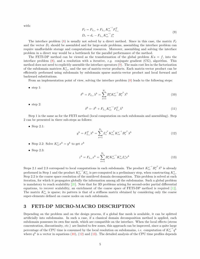
Let us consider two neighbouring subdomains Ωf and Ωc (fine and coarse, respectively) that are connectedon a local interface Γ, see Figure 3. Along this interface, the coarse subdomain shares only two corner nodes,which are common to the finely meshed subdomain.

fine mesh

side (f)

coarse mesh

side (c)

Ωf Ωc

Γ nf nodes

Figure 3: Interface of fine and coarse mesh

As a general rule, the mesh connection on the interface Γ, consists in satisfying the following continuityequation:

∀x ∈ Γ = Ωf ∩ Ωc, ufb (x) = ucb(x) (14)

where ufb (x) and ucb(x) are the continuous displacement fields on the fine and coarse sides of the interface Γ.

On the fine side, the continuous displacement field, ufb (x), is defined from the underlying fine mesh andthe shape functions of the corresponding elements. On the coarse side, the coarse element is built from anhomogenization process, and is defined with its coarse nodes. In order to define a continuous displacementfield on this coarse element, the shape functions corresponding to a classical finite element are used. In thiswork, since plate assemblies are considered, discrete Kirchhoff elements will be used, i.e. DKT or DKQ, seeAppendix 1. With these shape functions, the displacement vectors ucr and ucb are denoted as:

ucr = Ccucc

ucb = LcrCcucc

(15)

where Cc is the matrix of shape function values (interpolation matrix) on the coarse subdomain at thelocation of the fine mesh nodes, ucc is the displacement vector of subdomain Ωc at the coarse nodes and Lcr isthe localization matrix that restrict the degrees of freedom on the global incompatible interface, the cornernodes being excluded.

Several methods were presented in the literature to connect two incompatible meshes, such as collocation[22], Mortar [23], interface element method [24] as well as other approach discussed in [25]. The weak relationfor continuity of the displacement field at the subdomain interface can be written as follow:∫

Γ

w(x).(ufb (x)− ucb(x))dΓ = 0 (16)

where w is a weighting function. Different choices of w correspond to different types of connection.A micro-macro interpretation of the displacement fields is presented hereafter to guide the modeling

choice. For this purpose, the displacement field on the fine mesh is divided in two parts: a macroscopic part(ufMb ) and a microscopic part (ufmb ), as follow:

ufb (x) = ufMb (x) + ufmb (x) (17)

A classical choice consists to define the macro part (ufMb ) as the interpolation of the coarse field at the nodesof the fine mesh on the interface (ucb).

ufMb (x) = ucb(x) (18)

7

From Equations (17),(18), it can be seen that the connection between fine and coarse meshes amounts todefine locality constraints for the microscopic part of the displacement. Several approaches are discussedin [26], where macro and micro scales are superposed in the localization zone. In the work presented inthis paper, micro and macro scales are separated. Moreover, the approach is embedded in the FETI-DPframework. As a consequence, due to the strong continuity at the corner nodes, the microscopic field ufmbhas to be zero on these nodes.

Two types of connection are discussed here, which are based on the displacements (kinematic) and Mortar(static) approach.

4.1 Collocation method

The simplest way to satisfy the equation (16) consists of using the weighting function, w, as Dirac (δ)functions on the all nodes of the fine mesh side of the interface. Such a procedure will be called ‘collocation’.

This approach enforces the equality of the fine displacement field on one side, with the interpolation ofthe coarse displacement field on the other side:

ufb (xi) = ucb(xi) for i=1 to nf (19)

where nf is the number of interior interface nodes on the fine mesh side, see Figure 3.Taking into account (17) and (18), it yields for the microscopic displacement vector:

ufmb = 0 (20)

i.e. for all interior interface nodes on the fine mesh side, the micro displacement is null. Finally, fromufb = Bfr u

fr and using (15), the continuity equation (19) on the interface can be written in matrix form as:

Afufr = Dcucc (21)

where:Af = Bfr

Dc = LcrCc(22)

and ur, ub and uc are subdomain, interface and coarse nodes displacement vectors, respectively.

4.2 Mortar method

The Mortar method introduced in [23] is one rigorous and popular approach to enforce a weak continuity ofthe displacement field (16) at non-matching discrete interfaces. Within the framework of Mortar methods,the weighting function, w, plays the role of a Lagrange multiplier field, and a key point of the method is thespace of these Lagrange multipliers which has to be chosen carefully [27, 28]. A usual choice is a modifiedfinite element trace space of the coarsest mesh [27], with modifications concerning the end nodes of theinterface [23], which are here the coarse nodes shared by the two subdomains, see e.g. [18]. In the casestudied here with a coarse subdomain interface with only two nodes, if the shape functions are linear, theLagrange multiplier has to be taken as a constant.

For plate elements used in this work, the shape functions used for membrane degrees of freedom arelinear, while for bending the interpolation can be linear, quadratic, or cubic, see Appendix 1. However, forsake of simplicity, the Lagrange multiplier is chosen as a constant for each type of degree of freedom, oneach interface between two subdomains. It leads us to an average displacement connecting method on theinterface.

In this case, the displacement fields on the two sides of the interface satisfy the following relation:∫Γ

(ufb (x)− ucb(x))dΓ = 0 (23)

Here the same assumption are made as in (18), i.e. the macro displacement part of the fine side equalsthe interpolation of the coarse displacement fields on the coarse interface side. Therefore, with consideringequation (17), one obtains: ∫

Γ

ufmb (x)dΓ = 0 (24)

8

i.e. the average of the micro displacement part, ufmb , is null on the interface. It is recalled here that the

micro displacement ufmb is null at the corner node locations.The discretization of the gluing condition (23) leads to the linear constraint of the degrees of freedom on

two sides of the interface. The following notation is used again:

ufb (x) = N(x)ufb = N(x)Bfr ufr (x)

ucr = Ccucc

ucb(x) = N(x)Lcrucr = N(x)LcrCcu

cc

(25)

where for sake of simplicity, the continuous displacement fields, ufb (x) and ucb(x), are approximated usingpiecewise linear finite element shape function, N(x), defined on the interface fine mesh side.

Note that once the coarse displacement field has been interpolated (with matrix Cc), the same discretiza-tions are obtained for the coarse and fine sides of the interface. Therefore, the shape functions Nf and N c

on the two sides of the interface are the same and are denoted N .By substituting (25) in the equation (23), one obtains the following equation:∫

Γ

[N(x)Bfr ufr −N(x)LcrCcu

cc]dΓ = 0 (26)

And in the matrix form, it yields:

Afufr = Dcucc (27)

withAf = HBfr

Dc = HLcrCc

H =

∫Γ

N(x)dΓ

(28)

where H denotes the integral of the shape function on the interface.Disregarding the choice of the connection method, collocation or Mortar, the relation between the degrees

of freedom on the two sides of the interface can be put in similar forms (21) and (27). This relation is usedfor managing the incompatible interface constraints by domain decomposition method in the next Section.

5 Numerical homogenization of a finely meshed subdomain

In the previous section, two connection methods between incompatible displacement fields on the interfacebetween non-matching subdomains were presented. In this section, we are concerned with the determinationof an homogenized stiffness for coarse subdomains.

It is recalled there that the starting point of the method is a domain decomposition of the structurefrom subdomains with a fine mesh, compatible on the interface. Then, macro zones are chosen, and theircorresponding subdomains are described only from their coarse nodes, see Figure 2. When a subdomain isdiscretized at a macroscopic (homogenized) scale, a macroscopic stiffness should be associated to it. Thiscan be deduced from its fine discretization in a preliminary stage.

The critical step of any homogenization method lies in the localization step and concerns the way amacroscopic field loading is applied to the microscopic level. A main difficulty is the definition of suitedboundary conditions to be applied to the microscopic field on the micro domain. These boundary conditionscorrespond to a modeling of the loadings applied by the neighboring subdomains. Therefore, to ensure con-sistency of the FETI-DP micro-macro approach, the previous assumptions used for connection (collocationor Mortar) are applied again. These assumptions can be explained in the framework of homogenizationmethods. Thus, for the collocation approach, since the micro displacement field is supposed to be zero onthe subdomain boundary, this approach amounts to the strain approach of the Hill-Mandel method [29].For the Mortar method, the micro displacement field is constrained to be zero at the corner nodes. Theother boundary degrees of freedom are associated with a Lagrange multiplier which is constant. Thus there

9

are similarities with the stress approach of the Hill-Mandel method [29], in which uniform stress boundaryconditions are considered.

For a subdomain s, these boundary conditions were given by equations (15) and (19) (collocation) andequation (26) (Mortar) respectively, when fine and coarse mesh connection was treated. Since in the homog-enization process only one domain with a fine mesh is considered, they can be written in the general formof the equation (21) and (27) as follows:

Asusr = Dsusc (29)

Moreover, the internal degrees of freedom, which are free of any loading, are condensed statically on thecoarse ones. In this way, it is possible to derive a macro stiffness only defined on the coarse degrees offreedom. This homogenized stiffness is thus of a kinematic or static type, depending on the assumption usedfor the localization process.

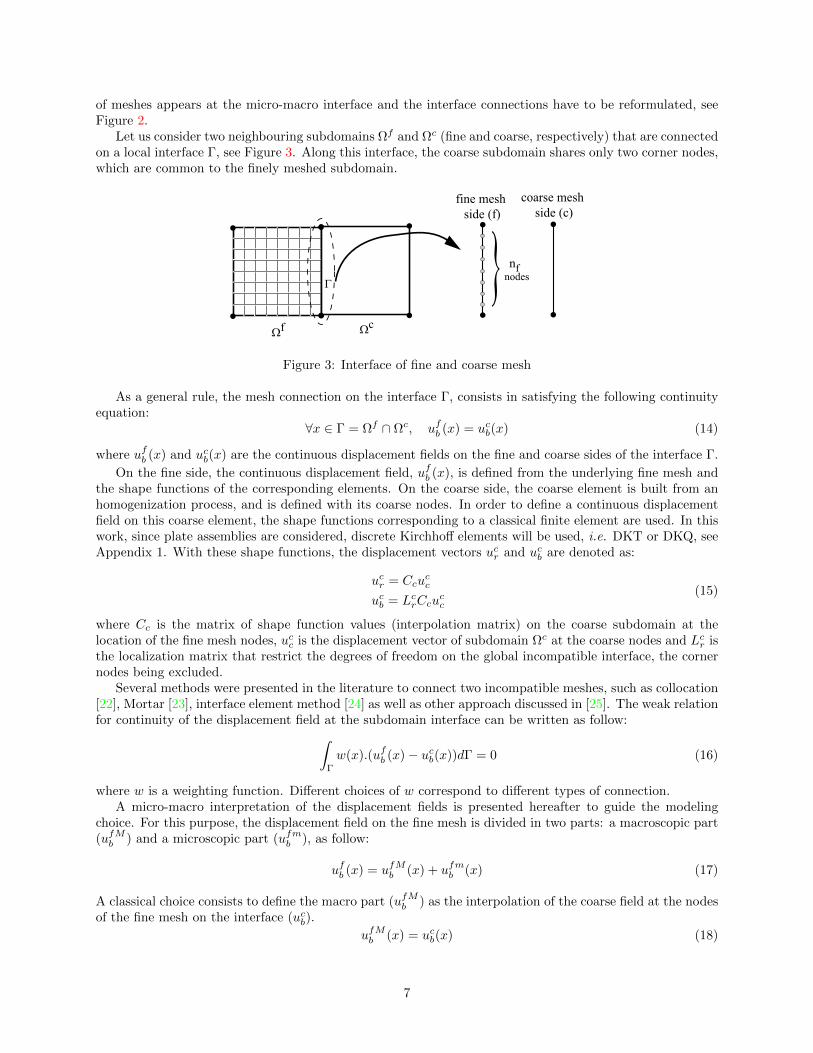
For each subdomain s, omitting the superscript s for simplification in the following, and considering theboundary conditions (29) on all the boundary of the subdomain, the equilibrium equation of this subdomainis:

∀ui, ub, uc, Aub = Duc,

uiubuc

T (

Kii Kib Kic

Kbi Kbb Kbc

Kci Kcb Kcc

uiubuc

− fifbfc

) = 0 (30)

where i, b and c still represent the subdomain internal, interface (non-corner) and corner degrees offreedom, respectively. One can enforce the boundary conditions by Lagrange multipliers in the equilibriumequations, which leads to:

Kii Kib Kic 0Kbi Kbb Kbc AT

Kci Kcb Kcc −DT

0 A −D 0

uiubucµ

−fifbfc0

= 0 (31)

The macroscopic stiffness on the corner degrees of freedom of the subdomain is obtained by condensing theinternal degrees of freedom ui, then in a second stage, ub and µ onto the coarse degrees of freedom uc.

As a result, one obtains the following expression for the macroscopic (homogenized) stiffness KH and themacroscopic (homogenized) consistent generalized force fH from the equilibrium equation (31):

KHuc = fH (32)

where:KH = (K?

cc + K?cbK

?−1

bb K?bc)

fH = f?c + K?cbK

?−1

bb f?b (33)

with:K?cc = K?

cc −K?cbK

?−1

bb K?bc

K?cb = DT +K?

cbK?−1

bb AT

K?bb = AK?−1

bb AT

f?c = f?c −K?cbK

?−1

bb f?b

f?b = AK?−1

bb f?b

(34)

and the terms obtained from the first condensation are:

K?cc = Kcc −KciK

−1ii Kic

K?cb = Kcb −KciK

−1ii Kib

K?bb = Kbb −KbiK

−1ii Kib

f?c = fc −KciK−1ii fi

f?b = fb −KbiK−1ii fb

(35)

These notations will be used in next Section to derive the new interface problem of the FETI-DP micro-macro approach.

10

6 FETI-DP MICRO-MACRO FORMULATION

Up to this point, three types of subdomain connections on the interface can be encountered, see Figure 2:

• connection of two subdomains with compatible fine meshes,

• connection of two subdomains with compatible coarse meshes,

• connection of the subdomains with incompatible fine and coarse meshes.

The first one is classical in FETI-DP method and the second one is satisfied automatically, since the coarsenodes are common between several subdomains. For the third one, the two methods (collocation and Mortar)presented previously, can be used. The different connections on the interfaces, once assembled for the wholeproblem, are:

Ns∑s=1

Bsrusr = 0 micro-micro connections

Ns∑s=1

(Asusr −Dsusc) = 0 micro-macro connections

(36)

Here, the formulation of the FETI-DP micro-macro method is presented by using the connections (36),the consistent macro stiffness matrix KH , and the generalized force vector fH , (33).

This can be achieved by introducing a second set of Lagrange multipliers, µ, for micro-macro interface,in addition to the classical Lagrange multipliers, λ, for micro-micro interface.

The unconstrained equilibrium equation for all the subdomains now reads:

∀usr, usc = Lscuc,∑s∈Nsf

[usrLscuc

]T ([Ksrr Ks

rc

Kscr Ks

cc

] [usrLscuc

]−[fsrfsc

])+∑s∈Nsc

(Lscuc)T (Ks

HLscuc − fsH) = 0 (37)

where Nsf and Nsc are the sets of subdomains with fine and coarse mesh, respectively.It should be noted that usr contains all degrees of freedom of a subdomain, other than the corners degrees

of freedom. So, for the macro subdomains, the degrees of freedom are restricted to usc.Using the interface continuity condition (36) in equation (37), it leads to:

Ksrru

sr +Ks

rcLscuc = fsr −Bs

T

r λ−AsT

µ for s=1, ... , Nsf (38)

and:

∑s∈Nsf

LsT

c Kscru

sr +

∑s∈Nsf

LsT

c KsccL

sc +

∑s∈Nsc

LsT

c KsHL

sc

uc =

∑s∈Nsf

LsT

c fsc +∑s∈Nsc

LsT

c fsH

+∑s∈Nsf

LsT

c DsT µ (39)

From equation (38) it follows that:

usr = Ks−1

rr (fsr −BsT

r λ−AsT

µ−KsrcL

scuc) (40)

Substituting equation (40) into equation (39) leads after some algebraic transformations to the new dual-primal interface problem with three unknowns (two Lagrange multipliers, λ and µ, and a primal displacementuc): −K?

cc Fcl FcmFlc Fll FlmFmc Fml Fmm

ucλµ

=

−f?cdldm

(41)

11

where:K?cc =

∑s∈Nsf

LsT

c KsccL

sc +

∑s∈Nsc

LsT

c KsHL

sc −

∑s∈Nsf

LsT

c KscrK

s−1

rr KsrcL

sc

Fll =∑s∈Nsf

BsrKs−1

rr BsT

r

Fmm =∑s∈Nsf

AsKs−1

rr AsT

andFcl =

∑s∈Nsf

LsT

c KscrK

s−1

rr BsT

r

Fcm =∑s∈Nsf

LsT

c (KscrK

s−1

rr AsT

+DsT )

Flm =∑s∈Nsf

BsrKs−1

rr AsT

and finally

f?c =∑s∈Nsf

LsT

c fsc +∑s∈Nsc

LsT

c F sH −∑s∈Nsf

LsT

c KscrK

s−1

rr fsr

dl =∑s∈Nsf

BsrKs−1

rr fsr

dm =∑s∈Nsf

AsKs−1

rr fsr

7 SOLUTION METHOD AND NUMERICAL EXAMPLES

Several approaches, in the context of substructure based iterative solver, already dealt with additionalconstraints with additional Lagrange multipliers, such as the incorporation of linear multipoint constraints[16, 17], and for FETI-DP formulation with Mortar constraints [30, 18].

Numerous techniques (outer iterations on µ, simultaneous iterations on λ and µ and outer iterations onλ) presented in [17, 16, 31], are used for solving the resulting problem (41).

In this article, the topic concerns mainly the modularity of the method. Therefore, the method ofsimultaneous iterations on λ and µ is chosen, which is the direct extension of the FETI-DP method, to solvethe interface problem (41) of the FETI-DP micro-macro method.

In a first step, the consistency of the FETI-DP micro-macro method is checked with patch tests. Afterthat, in the second step, several numerical examples (cantilever beam in bending, infinite plate with a holein traction and bending, etc.) are presented. Throughout the numerical examples, the results are comparedeither to an analytical solution or to a numerical reference solution (obtained with a classical finite elementmethod, with a fine mesh in all subdomains).

Two categories of FETI-DP micro-macro methods are considered in the following, according to theassumptions used for the connection of the fine and coarse mesh and the homogenization of the coarse mesh.A static approach where the Mortar method is used, and a kinematic one if the collocation approach ischosen. It is recalled at this point that collocation corresponds to the strain approach of the Hill-Mandelhomogenization theory, while the Mortar method presents similarities with the stress approach, see section5.

The first results of this approach were presented in [32] and [33].

7.1 Patch tests

Before applying the FETI-DP micro-macro method to different examples, one has to validate the two mainfeatures of the method, i.e. the connection between fine and coarse subdomains and the homogenizationused to derive the coarse subdomain stiffness. To this end, patch tests are now considered, with a uniform

12

state of stress and strain, and a membrane or bending loading. The examples are presented in Figure 4, witha pure traction and a pure bending case, in 2D and 3D respectively, and displacement boundary conditionsin order to prevent any rigid body displacement.

Exemple in bending

X

Y

Exemple in traction

X

Z Y

u=0v=0w=0 v=0

w=0

w=0

u=0v=0

v=0

Figure 4: Patch test with one subdomain

In a first step, the problem is solved using only one coarse domain. Its macro stiffness is computed fromthe static or kinematic homogenization of a fine mesh, as detailed in section 5. In both cases, and for themembrane and bending patch tests, the analytical displacement solution is recovered, up to the machineprecision for floating point computations.

X

Y

X

Y

Z

Figure 5: Patch test with an heterogeneous domain decomposition

In a second step, the same problems are considered, using the FETI-DP micro-macro proposed in thisarticle. Thus, an heterogeneous domain decomposition is studied, with fine and coarse subdomains, as shownin Figure 5. Fine mesh is used in the subdomain located in the center, while the others are described as acoarse subdomain with the macro stiffness obtained from homogenization of a fine mesh similar to that ofthe central domain. Once again, the analytical displacement solution is obtained, for membrane and bendingloadings, and for both types of methods, kinematic or static.

It can be noticed that the analytical solution of the problems studied in this section exhibits a uniformstate of stress (generalized stress for the bending case) and a zero micro displacement on the interface,according to the definition of equations (17) and (18). These situations are fully compatible with assumptionsused for the homogenization and connection between micro and macro subdomains, see equations (20) and(24). Therefore, it is logical that the the FETI-DP micro-macro approach passes the patch test.

More complicated examples will be considered in the following sections, in order to assess the approxi-mations of the FETI-DP micro-macro method, due to the homogenization of coarse subdomains and to theconnections between coarse and fine subdomains.

7.2 End loaded cantilever beam

In this subsection, an end-loaded cantilever beam, depicted in Figure 6, is studied. The loading consists ina parabolic shear force P and a linear traction force repartition at the end of the beam as follows:

• the shear forces (−P ) and (+P ) in y direction, with a parabolic distribution defined by (43), areimposed at two ends of the beam (at x = 0 and x = L, −H2 < y < H

2 ),

13

• at x = L, a linear force density in the x direction leads to a resultant bending moment (−M = −PL)in z direction, to balance the structure.

Displacement boundary conditions are also imposed at few nodes in order to prevent any rigid body motion,see Figure 6. The overall beam equilibrium provides the reactions which correspond to the force repartitionshown in Figure 6. The goal of this example is to study the global response of structure by FETI-DPmicro-macro method.

X

Y

par

abo

lic

forc

e

H

L

PP

M

O

A

X

Y

H

O

A

Figure 6: 2D cantilever beam in bending

This problem is bi-dimensional (plane stress) and the analytical solution is given e.g. in [34]. Thedisplacement is:

u(x, y) = −PyEI

[1

2(L2 − x2) +

(2 + ν)

6

(y2 − H2

4

)]v(x, y) = − P

EI

[L3

3− L2x

2+x3

6+

(4 + 5ν)

24H2(L− x) +

ν

2xy2] (42)

The stresses are given by:

σxx(x, y) =P

Ixy

σyy(x, y) = 0

σxy(x, y) =P

I

(H2

8− y2

2

) (43)

For the computations, the data used are, for the material parameters: Young’s modulus E = 1 GPa andPoisson’s ratio ν = 0.3. For the beam geometry, a unit thickness is considered, H = 4 m and L = 8 m. Theloading parameters are P = 7.5 × 105 N and M = 6 × 106 N.m, respectively. Finally the moment of inertiais I = H3/12.

In this example, the stress state is not uniform on the interface and in addition the micro displacement isnot zero on the micro-macro interface. These two conditions will check the homogenization and micro-macroconnection in the situation more severe than the patch test.

Let us consider the deflection in vertical direction at the point A, see Figure 6, for the two types of meshconnection and homogenization. For different number of subdomains, one consider half of them equippedwith a fine mesh, see Figure 7. The results are compared with the solution obtained with the uniformfine discretization (with a displacement −2.78× 10−2 m), see Figure 8, while the analytic reference value is−2.81× 10−2 m.

It can be seen that the FETI-DP micro-macro solution is in very good agreement with the analyticalsolution, even with a very small number of subdomains (one coarse and one fine). In the case of 8 subdomains(4 coarse and 4 fine subdomains) the relative difference on the global displacement of the point A is 3 % forthe kinematic case and 1.5 % for the static case.

14

A

A

A

Fine and coarse meshFine mesh

Figure 7: Decomposition in subdomains and micro-macro mesh (beam bending)

2 4 8

Dis

pla

cem

en

t (m

)

-3.20

-3.10

-3.00

-2.90

-2.80

-2.70

-2.60

-2.50

-2.40

-2.30

Number of subdomains

Kinematics approachStatic approachReference

x10-2

Figure 8: 2D beam with bending: displacement of the node A

15

7.3 An infinite plate with a hole in traction — plane stress study

The FETI-DP micro-macro method has been assessed in the previous example regarding overall results. Theobjective of the next example is to study the ability of the method to provide a good approximation of localresults. To this end, the example of a plate in traction with a circular hole is considered, see Figure 9. Largestress gradients are expected around the hole, and the method will be used limiting the subdomains witha fine discretization in the vicinity of this stress concentration zone, other zones being modeled with coarse(homogenized) mesh.

P

L

HP

eθer

a

AB

x

y

θ

Figure 9: Plate with a hole in traction and decomposition in subdomains

The plate is subjected to a uniform tension, P , in the x direction. The analytical solution in the case ofan infinite plate is presented in [34]. The stresses are given by the following relations:

σrr =P

2[(1− a2

r2) + (1− 4a2

r2+

3a4

r4) cos(2θ)]

σθθ =P

2[(1 +

a2

r2)− (1 +

3a4

r4) cos(2θ)]

σrθ =P

2[(1 +

2a2

r2− 3a4

r4) sin(2θ)]

(44)

where r and θ are the polar coordinates and the angle θ is measured from the positive x axis in the counter-clockwise direction. The maximum values of stress occur on the hole boundary and are given by:

σθθ(B) = σθθ(θ =π

2) = 3P

σθθ(A) = σθθ(θ = 0) = −P(45)

This analysis is based on the plane stress assumption. The isotropic material parameters are: Young’smodulus E = 210 GPa, and Poisson’s ration ν = 0.3. The following parameters are used for the plategeometry: L = 2.1 m , H = 2.1 m, r = 0.07 m and a unit thickness. The load value is p = 100 kN.

The parameters for the FETI-DP micro-macro method are 7× 7 subdomains, which means that the holediameter is close to half the subdomain length, see Figure 9. As a first step, the subdomain containing thehole is the only subdomain with a fine mesh. Since the studied plate is not infinite, a numerical referencesolution is computed with a fine mesh in all the subdomains. The FETI-DP micro-macro solution is thencompared to numerical and analytical reference solutions.

In order to assess the difference between the solution of the FETI-DP micro-macro method (with subscriptnum) and numerical reference solution (with subscript ref), we can define a relative energy norm of the error

16

3.78E−05 3.23E−02 6.46E−02 9.69E−02 0.13 0.16 0.19 0.23 0.26 0.29 0.32 0.36 0.39 0.42

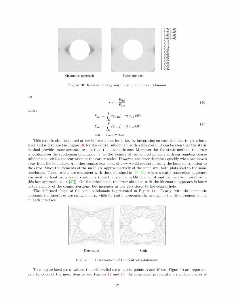
Kinematics approach Static approach

Figure 10: Relative energy norm error, 1 micro subdomain

as:

rΩ =Edif

Eref(46)

where:

Edif =

∫Ω

ε(udif) : σ(udif)dΩ

Eref =

∫Ω

ε(uref) : σ(uref)dΩ

udif = unum − uref

(47)

This error is also computed at the finite element level, i.e. by integrating on each element, to get a localerror and is displayed in Figure 10, for the central subdomain with a fine mesh. It can be seen that the staticmethod provides more accurate results than the kinematic one. Moreover, for the static method, the erroris localized on the subdomain boundary, i.e. in the vicinity of the connection zone with surrounding coarsesubdomains, with a concentration at the corner nodes. However, the error decreases quickly when one movesaway from the boundary. An other comparison point of view would consist in using the local contribution tothe error. Since the elements of the mesh are approximatively of the same size, both plots lead to the sameconclusion. These results are consistent with those obtained in [35, 36], where a static connection approachwas used, without using corner continuity (note that such an additional constraint can be also prescribed inthis last approach, as in [37]). On the other hand, the error obtained with the kinematic approach is lowerin the vicinity of the connection zone, but increases as one gets closer to the central hole.

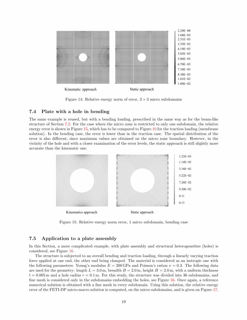
The deformed shape of the same subdomain is presented in Figure 11. Clearly, with the kinematicapproach the interfaces are straight lines, while for static approach, the average of the displacement is nullon each interface.

Kinematics Static

Figure 11: Deformation of the central subdomain

To compare local stress values, the orthoradial stress at the points A and B (see Figure 9) are reported,as a function of the mesh density, see Figures 12 and 13. As mentioned previously, a significant error is

17

obtained with the kinematic approach, while satisfactory results are given by the static approach, even ifthe size of the micro zone is only twice the hole diameter.

Str

ess

at n

od

e A

(M

Pa)

-1.2

-1.1

-1.0

-0.9

-0.8

-0.7

-0.6

6 x 6 12 x 12 20 x 20

Number of elements per subdomain

Kinematics approach

Static approach

Reference analytic

Reference numeric

-0.5

-0.4

-0.3

x 10+2

Figure 12: Infinite plate: stress at node A (σθθ)

Str

ess

at n

od

e B

(M

Pa)

2.0

2.2

2.4

2.6

2.8

3.0

3.2

6 x 6 12 x 12 20 x 20

Number of elements per subdomain

x 10+2

Kinematics approach

Static approach

Reference analytic

Reference numeric

Figure 13: Infinite plate: stress at node B (σθθ)

It can also be checked that for both methods, the error rapidly decreases when the size of the micro zoneincreases. Thus, for this problem and 7 × 7 subdomains again, the micro zone is now extended to 3 × 3subdomains at the center of the plate (instead of 1 in the previous example). The errors obtained with theFETI-DP micro-macro method are given in Figure 14, and are significantly smaller than those obtained withonly one micro subdomain, see Figure 10. For the kinematic method, the error still reaches its maximumvalue in the vicinity of the hole boundary.

18

2.29E−08

1.68E−03

2.51E−03

3.35E−03

4.19E−03

5.03E−03

5.86E−03

6.70E−03

7.54E−03

8.38E−03

1.01E−02

1.09E−02

Kinematic approach Static approach

Figure 14: Relative energy norm of error, 3× 3 micro subdomains

7.4 Plate with a hole in bending

The same example is reused, but with a bending loading, prescribed in the same way as for the beam-likestructure of Section 7.2. For the case where the micro zone is restricted to only one subdomain, the relativeenergy error is shown in Figure 15, which has to be compared to Figure 10 for the traction loading (membranesolution). In the bending case, the error is lower than in the traction case. The spatial distribution of theerror is also different, since maximum values are obtained on the micro zone boundary. However, in thevicinity of the hole and with a closer examination of the error levels, the static approach is still slightly moreaccurate than the kinematic one.

1.23E−03

1.14E−02

3.18E−02

5.22E−02

7.26E−02

9.30E−02

0.11

0.13

Kinematics approach Static approach

Figure 15: Relative energy norm error, 1 micro subdomain, bending case

7.5 Application to a plate assembly

In this Section, a more complicated example, with plate assembly and structural heterogeneities (holes) isconsidered, see Figure 16.

The structure is subjected to an overall bending and traction loading, through a linearly varying tractionforce applied at one end, the other end being clamped. The material is considered as an isotropic one withthe following parameters: Young’s modulus E = 200 GPa and Poisson’s ration ν = 0.3. The following dataare used for the geometry: length L = 3.0 m, breadth B = 2.0 m, height H = 2.0 m, with a uniform thicknesst = 0.005 m and a hole radius r = 0.1 m. For this study, the structure was divided into 36 subdomains, andfine mesh is considered only in the subdomains embedding the holes, see Figure 16. Once again, a referencenumerical solution is obtained with a fine mesh in every subdomain. Using this solution, the relative energyerror of the FETI-DP micro-macro solution is computed, on the micro subdomains, and is given on Figure 17.

19

L

B

H

A

Figure 16: Plate assembly subjected to an overall bending and traction loading (left), subdomains with fineand coarse meshes (right)

As previously, the accuracy of both static and kinematic approaches is satisfactory. For the static approach,the error is mainly located close to the coarse nodes, and decreases rapidly to a small value in the vicinityof the hole. The reverse is obtained for the kinematic approach.

5.03E−06

5.39E−03

1.08E−02

1.62E−02

2.15E−02

2.69E−02

3.23E−02

3.77E−02

4.31E−02

4.85E−02

5.38E−02

5.92E−02

6.46E−02

7.00E−02

StaticKinematics

Figure 17: Relative energy norm of error, plate assembly

8 CONCLUSIONS

In this article, a multi-scale extension of the FETI-DP method was presented for large-scale structuralanalysis. With this method, called FETI-DP micro-macro, different discretization scales can be used inthe subdomains, thanks to an homogenization step. Starting from a classical domain decomposition withmatching interfaces, most of the subdomains are homogenized, and the original mesh (fine mesh) is keptonly in the zones where local phenomena with high stress gradients are expected. One can then optimizethe computation time.

20

Two methods have been proposed for the connection of micro and macro subdomains on the interface: acollocation approach and a method which can be viewed as a limit case of the Mortar method. The interfacecontinuity is written in a weak sense, while corner continuity is enforced in a strong sense, due to the FETI-DP framework. These methods contrast with other connection approaches where the continuity is writtenon macro interface quantities, which are not classical degrees of freedom, see e.g. [35, 36]. In the sameway, two homogenization methods of the macro subdomains have been presented, with a localization processconsistent with the assumptions made for the connection process. Therefore, two FETI-DP micro-macroapproaches can be defined. Both were validated by using the patch tests.

The other numerical examples have shown that accurate results can be obtained from the proposedmethods. For a given problem, it turns out that the results are sensitive to the size of the micro zone. In thecase of a problem with structural heterogeneities, it means that the micro zone has to be large enough aroundthem. Both static and kinematic approaches exhibit errors in the vicinity of the incompatible interfaces.However, for the static approach, this can be considered as a boundary layer effect, since the error decreasesaway from the interfaces. The reverse is obtained for the kinematic approach. Thus, the static approachprovides more accurate results and appears to be more efficient than the kinematic one.

Concerning outlooks on this study, from a user point of view, automatic assessment of the error due tothe discretization [38] and to the scale description [39] would be of particular interest, as an indication todecide to change the scale modeling. This decision could also be done as an interactive way, during iterationsof the scheme to reach an adequate error level on the areas of interest. Obviously, the scale description isnot limited to two levels. A third level of description could also be used, for instance for a very local analysisof fatigue or crack propagation risk, which could also be performed with coupling the plate model with a 3Dmodel at the finest level.

Another interesting aspect to pursue this work is to adapt a specific preconditioner for the method ofsimultaneous iterations on λ and µ to solve the interface problem (see section 7). Several procedures havebeen proposed in the literature [17], that could be tested on the problem we are interested herein.

Appendix 1The stiffness matrix of the coarse elements are obtained from homogenization of a fine mesh. However, in

order to connect coarse element with surrounding micro subdomain, a continuous displacement field has tobe defined on its boundary. To this end, shape functions corresponding to a classical finite element (coarseelement) are chosen.

For the membrane behavior, a linear interpolation, is a good approximation for the in-plane displacements.But for the bending case with a Discrete Kirchhoff Triangle (DKT) and/or a Discrete Kirchhoff Quadrilateral(DKQ) plate element, the interpolation functions are cubic for the out-of-plane displacement w, quadraticfor the rotation denoted with θn, and linear for the rotation denoted with θt (t is the in-plane direction ofthe element edge, and n is the in-plane normal to the edge) [40], see Figure 18.

i

j

n

tz

θn

θt

Cubic Quadratic Linearwi wjθni θnj θti θtj

Figure 18: interpolation of the coarse field on the interface

Acknowledgements. The first author gratefully acknowledges the support of Iran’s Ministry of Science,Research and Technology and SFERE exchange program in France for financial supporting during his thesis.

21

References

[1] Y. Saad. Iterative Methods for Sparse Linear Systems. PWS Publishing Company, 1996.

[2] C. Farhat and F.-X. Roux. Implicit parallel processing in structural mechanics. Computational Me-chanics Advances, 2:1–121, 1994.

[3] I. Parsons and J. Hall. The multigrid method in solid mechanics: Part I, algorithm description andbehaviour. International Journal for Numerical Methods in Engineering, 29:719–737, 1990.

[4] I. Parsons and J. Hall. The multigrid method in solid mechanics: Part II, practical applications.International Journal for Numerical Methods in Engineering, 29:739–753, 1990.

[5] P. Vanek, M. Brezina, and J. Mandel. Convergence of algebraic multigrid based on smoothed aggrega-tion. Numerische Mathematik, 88:559–579, 2001.

[6] P. Gosselet and C. Rey. Non-overlapping domain decomposition methods in structural mechanics.Archives of Computational Methods in Engineering, 11-4:1–59, 2005.

[7] J. Mandel. Balancing domain decomposition. Communications in Applied Numerical Methods, 9:233–241, 1993.

[8] Ch. Farhat and F.-X. Roux. A method of finite element tearing and interconnecting and its parallelsolution algorithm. International Journal for Numerical Methods in Engineering, 32(6):1205–1227, 1991.

[9] L. Champaney, J.-Y. Cognard, D. Dureisseix, and P. Ladeveze. Large scale applications on parallelcomputers of a mixed domain decomposition method. Computational Mechanics, 19(4):253–263, 1997.

[10] K. C. Park, M. R. Justino, and C. A. Felippa. An algebraically partitioned FETI method for parallelstructural analysis: Algorithm description. International Journal for Numerical Methods in Engineering,40(15):2717–2737, 1997.

[11] D. J. Rixen, Ch. Farhat, R. Tezaur, and J. Mandel. Theoretical comparison of the FETI and algebraicallypartitioned FETI methods, and performance comparisons with a direct sparse solver. InternationalJournal for Numerical Methods in Engineering, 46:501–533, 1999.

[12] Ch. Farhat, M. Lesoinne, and K. Pierson. A scalable dual-primal domain decomposition method.Numerical Linear Algebra with Applications, 7:687–714, 2000.

[13] Ch. Farhat, M. Lesoinne, P. Le Tallec, K. Pierson, and D. Rixen. FETI-DP: A dual-primal unifiedFETI method – Part I: A faster alternative to the two-level FETI method. International Journal forNumerical Methods in Engineering, 50(7):1523–1544, 2001.

[14] Ch. Farhat, P. S. Chen, J. Mandel, and F.-X. Roux. The two-level FETI method – Part II: Extensionto shell problems, parallel implementation and performance results. Computer Methods in AppliedMechanics and Engineering, 155:153–180, 1998.

[15] M. Lesoinne. A FETI-DP corner selection algorithm for three-dimensional problems. In 14th Interna-tional Conference on Domain Decomposition Methods, pages 421–428, Mexico, 2002.

[16] Ch. Farhat, C. Lacour, and D. Rixen. Incorporation of linear multipoint constraints in substructurebased iterative solvers. Part 1: A numerically scalable algorithm. International Journal for NumericalMethods in Engineering, 43(6):997–1016, 1998.

[17] H. Bavestrello, Ph. Avery, and Ch. Farhat. Incorporation of linear multipoint constraints in domain-decomposition-based iterative solvers – Part II: Blending FETI-DP and mortar methods and assemblingfloating substructures. Computer Methods in Applied Mechanics and Engineering, 196:1347–1368, 2007.

[18] H. Kim. A FETI-DP formulation for compressible elasticity with mortar constraints. Lecture Notes inComputational Science and Engineering, 55:383–390, 2007.

22

[19] P. Le Tallec. Domain decomposition methods in computational mechanics. In Computational MechanicsAdvances, volume 1. North-Holland, 1994.

[20] J. H. Bramble, J. E. Pasciak, and A. H. Schatz. The construction of preconditioners for elliptic problemsby substructuring, I. Mathematics of Computation, 47(175):103–134, 1986.

[21] J. Sun, P. Michaleris, A. Gupta, and P. Raghavan. A fast implementation of the FETI-DP method:FETI-DP-RBS-LNA and applications on large scale problems with localized non linearities. Interna-tional Journal for Numerical Methods in Engineering, 63:833–858, 2005.

[22] D. Rixen. Substructuring and dual methods in structural analysis. Phd thesis, Universite de Liege,Faculte des Sciences Appliquees, 1997.

[23] C. Bernardi, Y. Maday, and A. Patera. A new nonconforming approach to domain decomposition: Themortar element method. College de France Seminar, pages 13–51, 1994.

[24] H. Kim. Interface element method (IEM) for a partitioned system with non-matching interfaces. Com-puter Methods in Applied Mechanics and Engineering, 191:3165–3194, 2002.

[25] P.-A. Guidault and T. Belytschko. On the L2 and H1 couplings for an overlapping domain decomposi-tion method using Lagrange multipliers. International Journal for Numerical Methods in Engineering,70:322–350, 2007.

[26] A. Hund and E. Ramm. Locality constraints within multiscale model for non-linear material behaviour.International Journal for Numerical Methods in Engineering, 70:1613–1632, 2007.

[27] B. Herry, L. Di Valentin, and A. Combescure. An approach to the connection between subdomains withnon-matching meshes for transient mechanical analysis. International Journal for Numerical Methodsin Engineering, 55(8):973–1003, 2002.

[28] P. Hauret and M. Oritz. BV estimates for mortar methods in linear elasticity. Computer Methods inApplied Mechanics and Engineering, 195:4783–4793, 2006.

[29] P. Suquet. Elements of homogenization for inelastic solid mechanics. In E. Sanchez-Palencia andA. Zaoui, editors, Homogenization Techniques for Composite Media, volume 272 of Lecture Notes inPhysics, pages 193–278. Springer-Verlag, Berlin, 1985.

[30] N. Dokeva. Scalable mortar methods for ellipic problems on many subregions. Phd thesis, Faculty ofthe graduate school University of Southern California, 2006.

[31] D. Rixen. Extended preconditioners for the FETI method applied to constrained problems. InternationalJournal for Numerical Methods in Engineering, 54:1–26, 2002.

[32] A. Mobasher Amini, D. Dureisseix, P. Cartraud, and N. Buannic. Multi-scale domain decompositionmethod for structural analysis of a passenger ship. In ECCOMAS Thematic Conference: Marine 2007— Computational Methods in Marine Engineering, Barcelona (Spain), june 2007.

[33] A. Mobasher Amini, D. Dureisseix, P. Cartraud, and N. Buannic. Analyse d’un navire a passagers avecune methode de decomposition de domaine a plusieurs echelles. In 8e Colloque National en Calcul desStructures, Giens, mai 2007. 6 p.

[34] S. Timoshenko and J. Goodier. Theory of elasticity. Mac Graw-Hill, third edition, 1970.

[35] P.-A. Guidault. Une strategie de calcul pour les structures fissurees : analyse locale-globale et approchemultiechelle pour la fissuration. PhD thesis, ENS Cachan, 2005.

[36] P.-A. Guidault, O. Allix, and J.-P. Navarro. A two-scale approach with homogenization for the compu-tation of cracked structures. Computers and Structures, 85(17-18):1360–1371, 2007.

[37] P. Alart and D. Dureisseix. A scalable multiscale LATIN method adapted to nonsmooth discrete media.Computer Methods in Applied Mechanics and Engineering, 197(5):319–331, 2008.

23

[38] P. Ladeveze and J.-P. Pelle. Mastering Calculations in Linear and Nonlinear Mechanics. Springer, 2004.

[39] J. T. Oden, K. Vemaganti, and N. Moes. Hierarchical modelling of heterogeneous solids. ComputerMethods in Applied Mechanics and Engineering, 172:3–25, 1999.

[40] J. Batoz and G. Dhatt. Modelisation des structures par elements finis, volume 2 – Poutres et Plaques.Hermes, Paris, 1993.

24