Ecological Complexity 22 (2015) 93–101

Original Research Article

Multi-scale comparison of topographic complexity indices in relationto plant species richness

Fangyuan Yu a,*, Tiejun Wang a,*, Thomas A. Groen a, Andrew K. Skidmore a, Xuefei Yang b,Yuying Geng c, Keping Ma c

a Department of Natural Resources, Faculty of Geo-Information Science and Earth Observation, University of Twente, Enschede 7500 AE, The Netherlandsb Laboratory of Biogeography and Biodiversity, Kunming Institute of Botany, Chinese Academy of Sciences, Kunming 650204, Chinac State Key Laboratory of Vegetation and Environmental Change, Institute of Botany, Chinese Academy of Sciences, Beijing 100093, China

A R T I C L E I N F O

Article history:

Received 8 September 2014

Received in revised form 7 February 2015

Accepted 9 February 2015

Available online 18 March 2015

Keywords:

Rhododendron

Biodiversity

Grain size

DEM

China

Topographic complexity

A B S T R A C T

Topographic complexity is a key component of habitat, which has been linked to increased species

richness in many ecological communities. It can be measured in various ways and it is unclear whether

these different measurements are mutually comparable when they relate to plant species richness at

different spatial scales. Using a densely sampled set of observations for Rhododendrons (406 species and

13,126 georeferenced records) as a test case, we calculated eight topographic complexity indices from a

250-m resolution digital elevation model and examined their correlations with Rhododendron species

richness in China at seven spatial scales: grain sizes 0.058, 0.18, 0.258, 0.58, 1.08, 1.58, and 2.08. Our results

showed that the eight topographic complexity indices were moderately to highly correlated with each

other, and the relations between each pair of indices decreased with increasing grain size. However, with

an increase in grain size, there was a higher correlation between topographic complexity indices and

Rhododendron species richness. At finer scales (i.e. grain size � 18), the standard deviation of elevation

and range of elevation had significantly stronger correlations with Rhododendron species richness than

other topographic complexity indices. Our findings indicate that different topographic complexity

indices may have positive correlations with plant species richness. Moreover, the topographic

complexity–species richness associations could be scale-dependent. In our case, the correlations

between topographic complexity and Rhododendron species richness tended to be stronger at coarse-

grained macro-habitat scales. We therefore suggest that topographic complexity index may serve as

good proxy for studying the pattern of plant species richness at continental to global levels. However,

choosing among topographic complexity indices must be undertaken with caution because these indices

respond differently to grain sizes.

� 2015 Elsevier B.V. All rights reserved.

Contents lists available at ScienceDirect

Ecological Complexity

jo ur n al ho mep ag e: www .e lsev ier . c om / lo cate /ec o co m

1. Introduction

Topographic complexity is a key component of habitat that hasbeen linked to species richness in many ecological communities,including terrestrial plants (Simpson, 1964; Bruun et al., 2006;Moeslund et al., 2013a; Stein et al., 2014). From the geomorpho-metric perspective, topography is always associated with eleva-tion, slope, aspect, and curvature, which in turn affect the waterand energy budgets of a location. This influences plant speciesdistribution and richness indirectly. Specifically, air temperature,atmospheric pressure, wind speed, season length, snow drift, snow

* Corresponding author at: PO Box 217, 7500 AE Enschede, The Netherlands.

Tel.: +31 53 4874227; fax: +31 53 4874388.

E-mail addresses: f.yu@utwente.nl (F. Yu), t.wang@utwente.nl (T. Wang).

http://dx.doi.org/10.1016/j.ecocom.2015.02.007

1476-945X/� 2015 Elsevier B.V. All rights reserved.

depth (Litaor et al., 2008), fog frequency (Svenning, 2001;Eiserhardt et al., 2011), and even human land use change withelevation (Franklin, 1998; Korner, 2007). Slope (gradient) affectsthe overland and subsurface flow velocity and runoff rate as well asthe soil water content (Gosz and Sharpe, 1989; Bispo et al., 2012),while terrain curvature is related to soil migration processes, wateraccumulation, and the movement of minerals and organicsubstances through the soil.

Many studies have used ‘‘topographic complexity’’ as a measureof topographic heterogeneity or even habitat heterogeneity, whichin turn have served as a proxy when exploring the determinants ofplant distribution and diversity patterns (Nichols et al., 1998; Kreftet al., 2006, 2010; Stein et al., 2014). The elevation range hasfrequently been used to express topographic complexity. Forexample, its effect has been demonstrated on palm speciesrichness (Kreft et al., 2006), mainland pteridophyte and seed

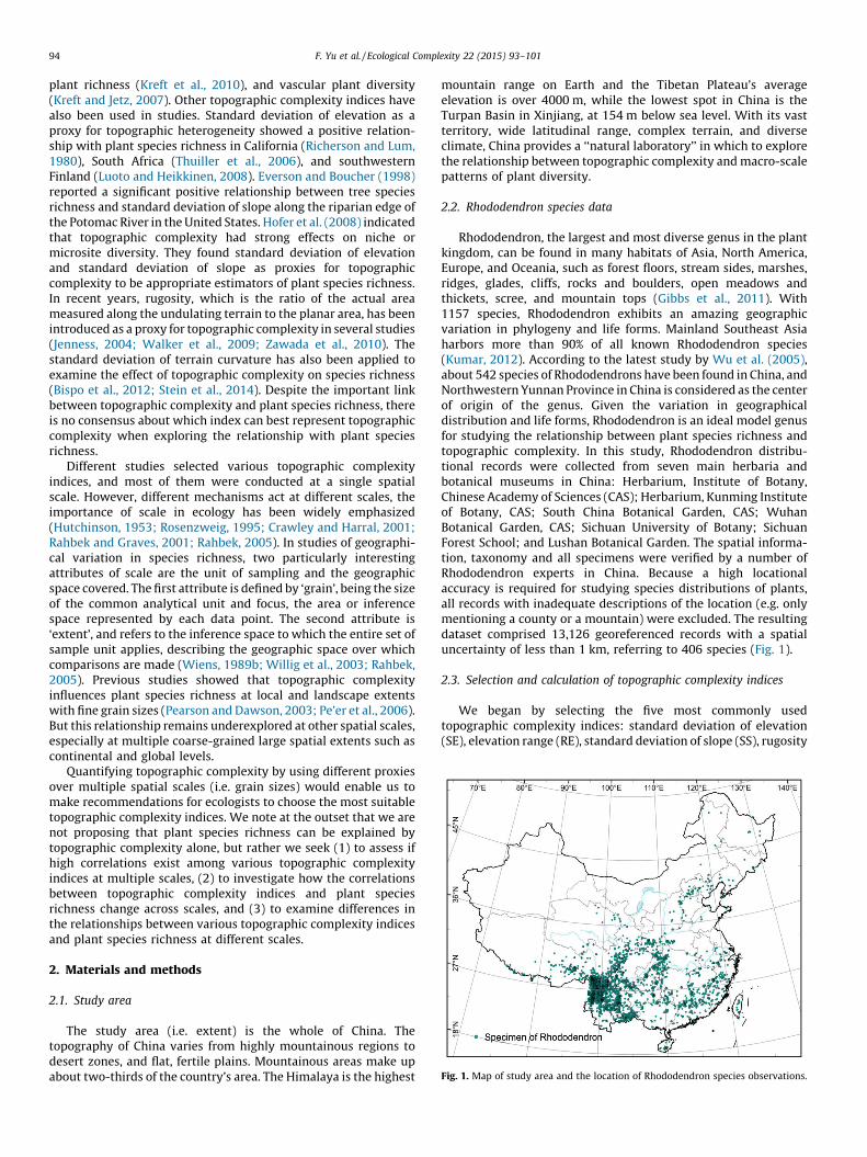
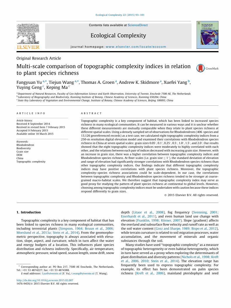
Fig. 1. Map of study area and the location of Rhododendron species observations.

F. Yu et al. / Ecological Complexity 22 (2015) 93–10194

plant richness (Kreft et al., 2010), and vascular plant diversity(Kreft and Jetz, 2007). Other topographic complexity indices havealso been used in studies. Standard deviation of elevation as aproxy for topographic heterogeneity showed a positive relation-ship with plant species richness in California (Richerson and Lum,1980), South Africa (Thuiller et al., 2006), and southwesternFinland (Luoto and Heikkinen, 2008). Everson and Boucher (1998)reported a significant positive relationship between tree speciesrichness and standard deviation of slope along the riparian edge ofthe Potomac River in the United States. Hofer et al. (2008) indicatedthat topographic complexity had strong effects on niche ormicrosite diversity. They found standard deviation of elevationand standard deviation of slope as proxies for topographiccomplexity to be appropriate estimators of plant species richness.In recent years, rugosity, which is the ratio of the actual areameasured along the undulating terrain to the planar area, has beenintroduced as a proxy for topographic complexity in several studies(Jenness, 2004; Walker et al., 2009; Zawada et al., 2010). Thestandard deviation of terrain curvature has also been applied toexamine the effect of topographic complexity on species richness(Bispo et al., 2012; Stein et al., 2014). Despite the important linkbetween topographic complexity and plant species richness, thereis no consensus about which index can best represent topographiccomplexity when exploring the relationship with plant speciesrichness.

Different studies selected various topographic complexityindices, and most of them were conducted at a single spatialscale. However, different mechanisms act at different scales, theimportance of scale in ecology has been widely emphasized(Hutchinson, 1953; Rosenzweig, 1995; Crawley and Harral, 2001;Rahbek and Graves, 2001; Rahbek, 2005). In studies of geographi-cal variation in species richness, two particularly interestingattributes of scale are the unit of sampling and the geographicspace covered. The first attribute is defined by ‘grain’, being the sizeof the common analytical unit and focus, the area or inferencespace represented by each data point. The second attribute is‘extent’, and refers to the inference space to which the entire set ofsample unit applies, describing the geographic space over whichcomparisons are made (Wiens, 1989b; Willig et al., 2003; Rahbek,2005). Previous studies showed that topographic complexityinfluences plant species richness at local and landscape extentswith fine grain sizes (Pearson and Dawson, 2003; Pe’er et al., 2006).But this relationship remains underexplored at other spatial scales,especially at multiple coarse-grained large spatial extents such ascontinental and global levels.

Quantifying topographic complexity by using different proxiesover multiple spatial scales (i.e. grain sizes) would enable us tomake recommendations for ecologists to choose the most suitabletopographic complexity indices. We note at the outset that we arenot proposing that plant species richness can be explained bytopographic complexity alone, but rather we seek (1) to assess ifhigh correlations exist among various topographic complexityindices at multiple scales, (2) to investigate how the correlationsbetween topographic complexity indices and plant speciesrichness change across scales, and (3) to examine differences inthe relationships between various topographic complexity indicesand plant species richness at different scales.

2. Materials and methods

2.1. Study area

The study area (i.e. extent) is the whole of China. Thetopography of China varies from highly mountainous regions todesert zones, and flat, fertile plains. Mountainous areas make upabout two-thirds of the country’s area. The Himalaya is the highest

mountain range on Earth and the Tibetan Plateau’s averageelevation is over 4000 m, while the lowest spot in China is theTurpan Basin in Xinjiang, at 154 m below sea level. With its vastterritory, wide latitudinal range, complex terrain, and diverseclimate, China provides a ‘‘natural laboratory’’ in which to explorethe relationship between topographic complexity and macro-scalepatterns of plant diversity.

2.2. Rhododendron species data

Rhododendron, the largest and most diverse genus in the plantkingdom, can be found in many habitats of Asia, North America,Europe, and Oceania, such as forest floors, stream sides, marshes,ridges, glades, cliffs, rocks and boulders, open meadows andthickets, scree, and mountain tops (Gibbs et al., 2011). With1157 species, Rhododendron exhibits an amazing geographicvariation in phylogeny and life forms. Mainland Southeast Asiaharbors more than 90% of all known Rhododendron species(Kumar, 2012). According to the latest study by Wu et al. (2005),about 542 species of Rhododendrons have been found in China, andNorthwestern Yunnan Province in China is considered as the centerof origin of the genus. Given the variation in geographicaldistribution and life forms, Rhododendron is an ideal model genusfor studying the relationship between plant species richness andtopographic complexity. In this study, Rhododendron distribu-tional records were collected from seven main herbaria andbotanical museums in China: Herbarium, Institute of Botany,Chinese Academy of Sciences (CAS); Herbarium, Kunming Instituteof Botany, CAS; South China Botanical Garden, CAS; WuhanBotanical Garden, CAS; Sichuan University of Botany; SichuanForest School; and Lushan Botanical Garden. The spatial informa-tion, taxonomy and all specimens were verified by a number ofRhododendron experts in China. Because a high locationalaccuracy is required for studying species distributions of plants,all records with inadequate descriptions of the location (e.g. onlymentioning a county or a mountain) were excluded. The resultingdataset comprised 13,126 georeferenced records with a spatialuncertainty of less than 1 km, referring to 406 species (Fig. 1).

2.3. Selection and calculation of topographic complexity indices

We began by selecting the five most commonly usedtopographic complexity indices: standard deviation of elevation(SE), elevation range (RE), standard deviation of slope (SS), rugosity

F. Yu et al. / Ecological Complexity 22 (2015) 93–101 95

(RU), and standard deviation of curvature (SC). These five indicesdepict topography from different perspectives and have been usedas proxies for topographic complexity in previous studiesexploring the underlying mechanisms of plant species richness.In addition to these indices, we included two less studied butpotentially important topographic complexity indices: slope range(SR) and the compound terrain complexity index (CTCI). SRexpresses the variability of slope, which affects the velocity of bothsurface and subsurface flow and hence soil water content, erosionpotential, soil formation, and many other important processes(Gallant and Wilson, 2000). CTCI, deduced from four indices(standard deviation of elevation, elevation range, total curvature,and rugosity) is a synthetic index that comprises different featuresof topography and so can be used to evaluate several aspects oftopographic complexity simultaneously (Lu et al., 2007). Our studyis the first to test the relationship between CTCI and plant speciesrichness.

Principal component analysis (PCA) is one of the most commonmethods for detecting multi-collinearity in a variable set and toreduce the number of variables in data analysis (Austin, 2002;Svenning et al., 2010; Wang et al., 2012; Barbosa et al., 2014). It canbe used to select the variables that contain the most information.Based on the results of a principal component analysis of the sixfundamental topographic complexity indices (i.e. SE, RE, SS, RS, SC,and RU), we adopted the first principal component which accountsfor over 80% of the variance in the data as a new topographiccomplexity index (i.e. PCA) in our study. The definition andequations of all above-mentioned eight indices are given in Table 1.

The Digital Elevation Model (DEM) used to calculate thetopographic complexity indices was derived from the USGS GlobalMulti-Resolution Terrain Elevation Data 2010 (http://topotools.cr.usgs.gov/gmted_viewer/), with a spatial resolution of 250 m. Slopewas computed using the Slope Tool in the spatial analysis moduleof ArcGIS 10.0 (ESRI, Inc., Redlands, California, USA). The terraincurvature (hereafter referred to as ‘‘curvature’’), total curvature,and rugosity were calculated with the DEM Surface Tool, anextension for ArcGIS10.0 (http://www.jennessent.com/arcgis/surface_area.htm). Subsequently, using elevation, slope, andcurvature as primary input data and the Zonal Statistics Tool inArcGIS 10.0 we calculated the standard deviation of elevation,range of elevation, standard deviation of slope, range of slope, andstandard deviation of curvature. Lastly, we calculated CTCI withthe algorithm developed by Lu et al. (2007). Maps of topographiccomplexity indices in China with a grain size of 0.58 are displayed

Table 1Description of topographic complexity indices.

Index Unit Abbr. Definition

Standard deviation of

elevation

m SE A measure of the variability of el

the circular window. It measures

of the landscape at the coarser

Range of elevation m RE Arithmetic difference between t

and minimum elevations

Standard deviation of

slope

degree SS Standard deviation of slope

Range of slope degree RS A measure of the ‘‘relief of slope’

Standard deviation of

curvature

radians per

square meter

SC Description the variation of the

that surface is merely flat or hil

Rugosity – RU The ratio of surface area (As) to

(Ap); describes how wrinkled a

Compound terrain

complexity index

– CTCI Weights four indices that depict

complexity from different persp

Principal component

analysis

– PCA The first principal component o

fundamental topographic compl

(i.e. SE, RE, SS, RS, SC and RU)

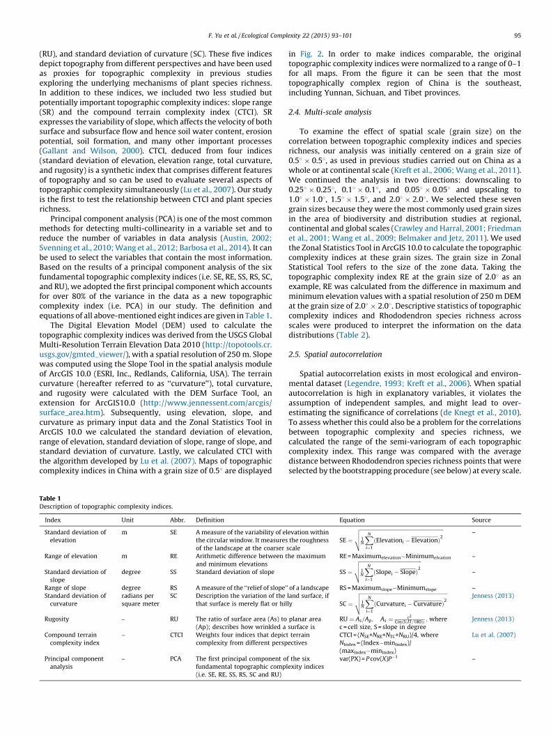
in Fig. 2. In order to make indices comparable, the originaltopographic complexity indices were normalized to a range of 0–1for all maps. From the figure it can be seen that the mosttopographically complex region of China is the southeast,including Yunnan, Sichuan, and Tibet provinces.

2.4. Multi-scale analysis

To examine the effect of spatial scale (grain size) on thecorrelation between topographic complexity indices and speciesrichness, our analysis was initially centered on a grain size of0.58 � 0.58, as used in previous studies carried out on China as awhole or at continental scale (Kreft et al., 2006; Wang et al., 2011).We continued the analysis in two directions: downscaling to0.258 � 0.258, 0.18 � 0.18, and 0.058 � 0.058 and upscaling to1.08 � 1.08, 1.58 � 1.58, and 2.08 � 2.08. We selected these sevengrain sizes because they were the most commonly used grain sizesin the area of biodiversity and distribution studies at regional,continental and global scales (Crawley and Harral, 2001; Friedmanet al., 2001; Wang et al., 2009; Belmaker and Jetz, 2011). We usedthe Zonal Statistics Tool in ArcGIS 10.0 to calculate the topographiccomplexity indices at these grain sizes. The grain size in ZonalStatistical Tool refers to the size of the zone data. Taking thetopographic complexity index RE at the grain size of 2.08 as anexample, RE was calculated from the difference in maximum andminimum elevation values with a spatial resolution of 250 m DEMat the grain size of 2.08 � 2.08. Descriptive statistics of topographiccomplexity indices and Rhododendron species richness acrossscales were produced to interpret the information on the datadistributions (Table 2).

2.5. Spatial autocorrelation

Spatial autocorrelation exists in most ecological and environ-mental dataset (Legendre, 1993; Kreft et al., 2006). When spatialautocorrelation is high in explanatory variables, it violates theassumption of independent samples, and might lead to over-estimating the significance of correlations (de Knegt et al., 2010).To assess whether this could also be a problem for the correlationsbetween topographic complexity and species richness, wecalculated the range of the semi-variogram of each topographiccomplexity index. This range was compared with the averagedistance between Rhododendron species richness points that wereselected by the bootstrapping procedure (see below) at every scale.

Equation Source

evation within

the roughness

scale

SE ¼

ffiffiffiffiffiffiffiffiffiffiffiffiffiffiffiffiffiffiffiffiffiffiffiffiffiffiffiffiffiffiffiffiffiffiffiffiffiffiffiffiffiffiffiffiffiffiffiffiffiffiffiffiffiffiffiffiffiffiffiffiffiffiffiffiffi1N

XN

i¼1

ðElevationi � ElevationÞ2vuut

–

he maximum RE = Maximumelevation�Minimumelvation –

SS ¼

ffiffiffiffiffiffiffiffiffiffiffiffiffiffiffiffiffiffiffiffiffiffiffiffiffiffiffiffiffiffiffiffiffiffiffiffiffiffiffiffiffiffiffiffiffiffiffiffi1N

XN

i¼1

ðSlopei � SlopeÞ2vuut –

’ of a landscape RS = Maximumslope�Minimumslope –

land surface, if

ly SC ¼

ffiffiffiffiffiffiffiffiffiffiffiffiffiffiffiffiffiffiffiffiffiffiffiffiffiffiffiffiffiffiffiffiffiffiffiffiffiffiffiffiffiffiffiffiffiffiffiffiffiffiffiffiffiffiffiffiffiffiffiffiffiffiffiffiffiffiffiffi1N

XN

i¼1

ðCurvaturei � CurvatureÞ2vuut

Jenness (2013)

planar area

surface is

RU ¼ As=Ap; As ¼ c2

CosðSðP=180ÞÞ ; where

c = cell size, S = slope in degree

Jenness (2013)

terrain

ectives

CTCI = (NSE+NRE+NTC+NRU)/4, where

NIndex = (Index�minIndex)/

(maxIndex�minIndex)

Lu et al. (2007)

f the six

exity indices

var(PX) = P cov(X)P�1 –

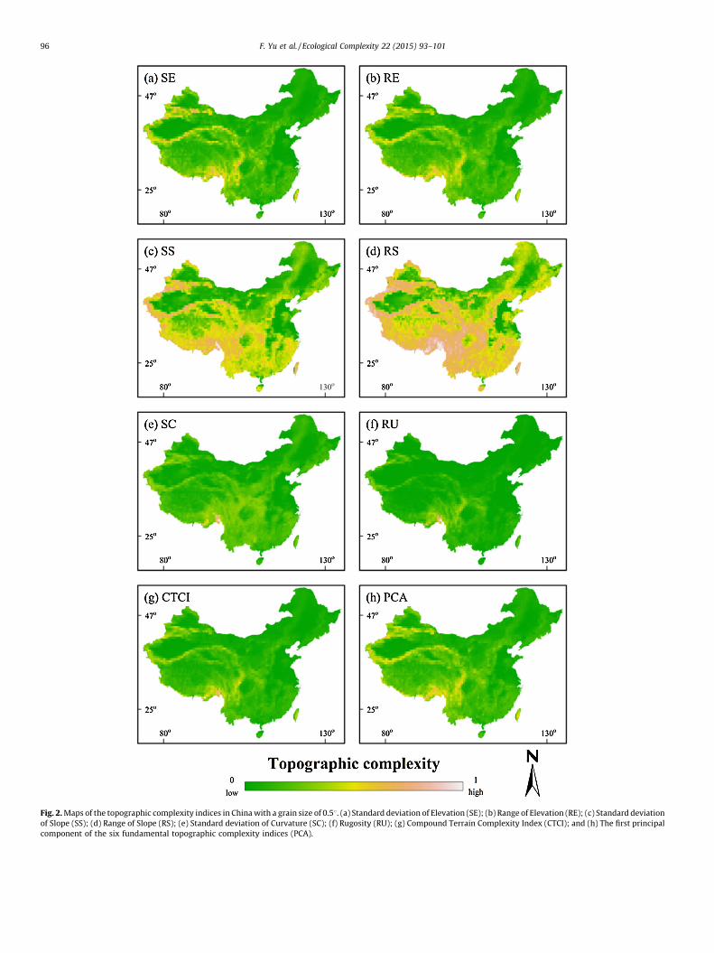
Fig. 2. Maps of the topographic complexity indices in China with a grain size of 0.58. (a) Standard deviation of Elevation (SE); (b) Range of Elevation (RE); (c) Standard deviation

of Slope (SS); (d) Range of Slope (RS); (e) Standard deviation of Curvature (SC); (f) Rugosity (RU); (g) Compound Terrain Complexity Index (CTCI); and (h) The first principal

component of the six fundamental topographic complexity indices (PCA).

F. Yu et al. / Ecological Complexity 22 (2015) 93–10196

Table 2Summary of statistics (mean � SD) of the eight topographic complexity indices and the species richness (SP) of Rhododendrons at grain sizes of 0.058, 0.18, 0.258, 0.58, 1.08, 1.58, and

2.08.

Index Scale

0.058 0.18 0.258 0.58 1.08 1.58 2.08

SE 221.92 � 128.51 287.47 � 162.83 334.35 � 187.08 335.22 � 192.66 341.17 � 202.14 376.55 � 262.76 384.52 � 261.62

RE 981.28 � 524.80 1330.32 � 676.34 1702.65 � 830.76 1913.36 � 980.98 2148.86 � 1120.15 2443.87 � 1320.96 2636.32 � 1400.22

SS 8.52 � 2.44 8.97 � 2.21 9.23 � 2.20 9.15 � 2.35 8.98 � 2.56 9.02 � 2.72 8.85 � 2.86

RS 41.99 � 10.90 46.97 � 10.05 51.61 � 9.55 54.07 � 9.53 56.11 � 9.66 58.18 � 10.07 58.87 � 10.49

SC 0.08 � 0.03 0.08 � 0.03 0.08 � 0.03 0.07 � 0.03 0.07 � 0.03 0.06 � 0.03 0.06 � 0.03

RU 1.08 � 0.06 1.08 � 0.06 1.07 � 0.06 1.06 � 0.05 1.05 � 0.04 1.05 � 0.04 1.04 � 0.04

CTCI 0.11 � 0.06 0.14 � 0.07 0.15 � 0.09 0.16 � 0.10 0.17 � 0.11 0.17 � 0.11 0.19 � 0.12

PCA 2.96 � 2.20 2.91 � 2.12 2.48 � 2.04 1.89 � 2.00 1.26 � 1.91 1.05 � 1.98 0.72 � 2.00

SP 3.28 � 5.07 3.96 � 5.99 5.81 � 8.52 8.05 � 12.20 11.18 � 16.08 14.21 � 20.12 19.10 � 27.97

For abbreviations of topographic complexity indices, see Table 1.

F. Yu et al. / Ecological Complexity 22 (2015) 93–101 97

2.6. Statistical analysis

Pearson’s correlation coefficient (r) was calculated for everycombination of topographic complexity indices and betweentopographic complexity indices and Rhododendron species rich-ness. To increase the stability and reliability of the correlations, weapplied a bootstrapping procedure to calculate an averagecorrelation from 500 bootstrapped samples, each consisting of100 sampling units (Pattengale et al., 2009). We fixed the samplingsize at 100 because at the coarsest grain size (2.08) this was themaximum number of pixels available, given the spatial extent(China) of the study. By fixing the sample size over all scales,possible changes observed between the bootstrapped correlationsmay be attributed to the scale rather than to the variation insample size between scales.

To compare the correlations between all combinations oftopographic complexity indices and between Rhododendronspecies richness and topographic complexity indices at differentscales, a Games-Howell post hoc test after a one-way ANOVAwas used. All statistical analyses were implemented in the Rsoftware environment (version 2.15.3, R Development CoreTeam).

Fig. 3. Cross-correlation matrix of eight topographic complexity indic

3. Results

3.1. Spatial correlation of topographic complexity indices at multiple

scales

The eight topographic complexity indices were moderately tohighly correlated with each other (Fig. 3). The correlations betweeneach pair of indices decreased with increasing grain size. Ingeneral, higher correlations can be found between SE, RE, and CTCI.By contrast, RU and SC had lower correlations with other indices.

3.2. Correlation between topographic complexity indices and

Rhododendron species richness across scales

The average correlations from 500 repeated bootstrappinganalyses showed that the eight topographic complexity indiceshad significantly positive correlations with Rhododendron speciesrichness from 0.258 to 2.08, but no significant correlations at scalesof 0.058 and 0.18. With an increase in grain size, the associationbetween the eight topographic complexity indices and Rhododen-dron species richness changed (Table 3). Two groups of indicesemerged. The first was the ‘‘elevation group’’ (SE and RE): its

es at different scales. All correlations are significant at p < 0.01.

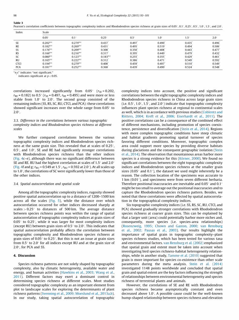
Table 3Pearson’s correlation coefficients between topographic complexity indices and Rhododendron species richness at grain sizes of 0.058, 0.18, 0.258, 0.58, 1.08, 1.58, and 2.08.

Index Scale

0.058 0.18 0.258 0.58 1.08 1.58 2.08

SE 0.202n.s 0.279n.s 0.437* 0.497* 0.490* 0.435* 0.496*

RE 0.182n.s 0.269n.s 0.431* 0.495* 0.519* 0.494* 0.506*

SS 0.176n.s 0.209n.s 0.308* 0.350* 0.408* 0.443* 0.477*

RS 0.166n.s 0.216n.s 0.317* 0.395* 0.449* 0.479* 0.432*

SC 0.080n.s 0.123n.s 0.183n.s 0.255* 0.355* 0.429* 0.461*

RU 0.165n.s 0.222n.s 0.312* 0.386* 0.471* 0.549* 0.592*

CTCI 0.194n.s 0.279n.s 0.408* 0.459* 0.497* 0.510* 0.549*

PCA 0.181n.s 0.252n.s 0.368* 0.439* 0.490* 0.524* 0.548*

‘‘n.s’’ indicates ‘‘not significant.’’* indicates significant at p < 0.05.

F. Yu et al. / Ecological Complexity 22 (2015) 93–10198

correlations increased significantly from 0.058 (rSE = 0.202,rRE = 0.182) to 0.58 (rSE = 0.497, rRE = 0.495) and were more or lessstable from 1.08 to 2.08. The second group consisted of theremaining indices (SS, RS, SC, RU, CTCI, and PCA): these correlationsshowed significant increases over the whole range from 0.058 to2.08.

3.3. Difference in the correlations between various topographic

complexity indices and Rhododendron species richness at different

scales

We further compared correlations between the varioustopographic complexity indices and Rhododendron species rich-ness at the same grain size. This revealed that at scales of 0.258,0.58, and 1.08, SE and RE had significantly stronger correlationswith Rhododendron species richness than the other indices(Fig. 4c–e), although there was no significant difference betweenSE and RE. RU had the highest correlation at scales of 1.58 and 2.08(Fig. 4f and g; rRU = 0.549 at 1.58, rRU = 0.592 at 2.08). At all scales upto 1.08, the correlations of SC were significantly lower than those ofthe other indices.

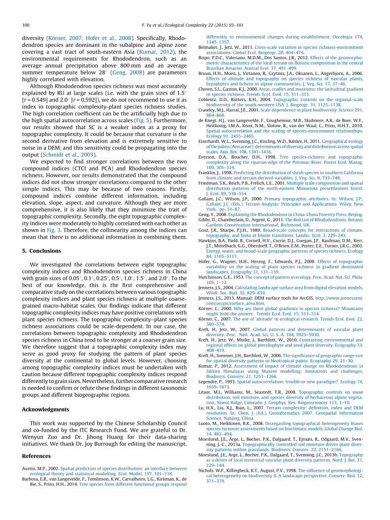
3.4. Spatial autocorrelation and spatial scale

Among all the topographic complexity indices, rugosity showedpositive spatial autocorrelation up to a distance of 1200–1500 kmacross all the scales (Fig. 5), while the distance over whichautocorrelation occurred for other indices decreased sharply atscales > 0.258 to distances of 500 km. The average distancebetween species richness points was within the range of spatialautocorrelation of topographic complexity indices at grain sizes of0.058 to 0.258, while it was larger for most complexity indices(except RU) between grain sizes of 0.58 to 2.08. This indicates thatspatial autocorrelation probably affects the correlation betweentopographic complexity and Rhododendron species richness atgrain sizes of 0.058 to 0.258. But this is not an issue at grain sizesfrom 0.58 to 2.08 for all indices except RU and at the grain size of2.08, for PCA and SS.

4. Discussion

Species richness patterns are not solely shaped by topographiccomplexity, also by climatic heterogeneity, available water andenergy, and human activities (Hawkins et al., 2003; Wang et al.,2011). Different factors may exert a dominant control indetermining species richness at different scales. Most studiesconsidered topographic complexity as an important element fromplot to landscape scales for exploring the determinants of plantrichness patterns (Svenning et al., 2009; Moeslund et al., 2013a,b).In our study, taking spatial autocorrelation of topographic

complexity indices into account, the positive and significantcorrelations between the eight topographic complexity indices andRhododendron species richness in China across large grain sizes(i.e. 0.58, 1.08, 1.58, and 2.08) indicate that topographic complexityinfluences plant species richness at regional to continental scalesas well, which is in accordance with previous studies (Coblentz andRiitters, 2004; Kreft et al., 2006; Eiserhardt et al., 2011). Thepositive correlations can be a consequence of the combined effectof different mechanisms, including promotion of species coexis-tence, persistence and diversification (Stein et al., 2014). Regionswith more complex topographic conditions have steep climaticand habitat gradients promoting spatial turnover of speciesfavoring different conditions. Moreover, topographic complexarea could support more species by providing diverse habitatsduring glaciations and the consequent geographic isolation (Steinet al., 2014). The observation that mountainous areas harbor morespecies is a strong evidence for this (Korner, 2000). We found nosignificant correlations between the eight topographic complexityindices and Rhododendron species richness at the smaller grainsizes (0.058 and 0.18), the dataset we used might inherently be areason. The collection location of the specimens was accurate to1 km (0.018), and specimens were from seven different herbaria.Therefore positional inaccuracies are inevitable and 0.058 and 0.18might be too small to average out the positional inaccuracies and tocapture the Rhododendron species richness pattern. Besides, wenoted that these correlations were affected by spatial autocorrela-tion in the topographical complexity indices.

Six topographic complexity indices (i.e. SS, RS, SC, RU, CTCI, andPCA) showed gradually stronger correlations with Rhododendronspecies richness at coarser grain sizes. This can be explained bythat a larger unit (area) could potentially harbor more niches and,consequently, more species (i.e. species-area relationships)(Rosenzweig, 1995; Chown and Gaston, 2000; van Rensburget al., 2002; Pausas et al., 2003). Our results highlight theimportance of spatial grain in topographic complexity–plantspecies richness studies, which has been tested for various taxaand environmental factors. van Rensburg et al. (2002) emphasizedthat spatial grain and extent must be taken into account wheninvestigating bird species richness-habitat heterogeneity relation-ships, while in another study, Tamme et al. (2010) suggested thatgrain is more important for species co-existence than other scaleparameters during the meta analysis. Stein et al. (2014)investigated 1148 points worldwide and concluded that spatialgrain and spatial extent are the key factors influencing the strengthof relationships between environmental heterogeneity and speciesrichness of terrestrial plants and animals.

However, the correlations of SE and RE with Rhododendronspecies richness became asymptotically constant and evendecreased above 1.08. A possible cause could be the well-knownhump-shaped relationship between species richness and elevation

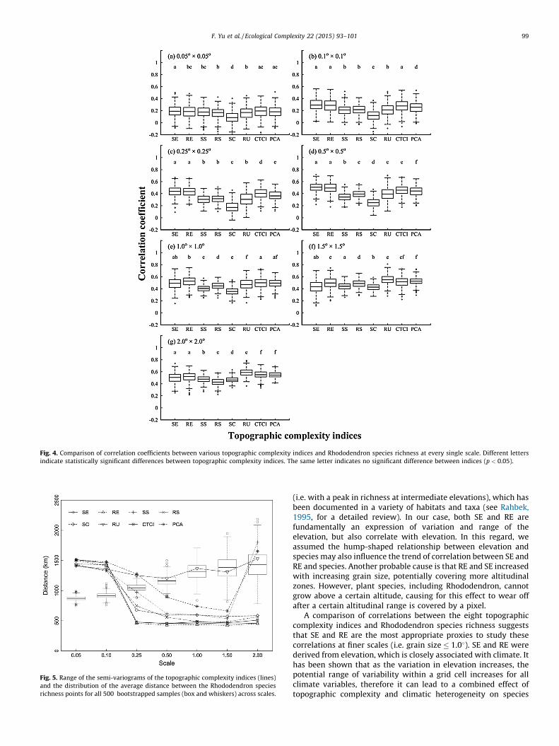
Fig. 5. Range of the semi-variograms of the topographic complexity indices (lines)

and the distribution of the average distance between the Rhododendron species

richness points for all 500 bootstrapped samples (box and whiskers) across scales.

Fig. 4. Comparison of correlation coefficients between various topographic complexity indices and Rhododendron species richness at every single scale. Different letters

indicate statistically significant differences between topographic complexity indices. The same letter indicates no significant difference between indices (p < 0.05).

F. Yu et al. / Ecological Complexity 22 (2015) 93–101 99

(i.e. with a peak in richness at intermediate elevations), which hasbeen documented in a variety of habitats and taxa (see Rahbek,1995, for a detailed review). In our case, both SE and RE arefundamentally an expression of variation and range of theelevation, but also correlate with elevation. In this regard, weassumed the hump-shaped relationship between elevation andspecies may also influence the trend of correlation between SE andRE and species. Another probable cause is that RE and SE increasedwith increasing grain size, potentially covering more altitudinalzones. However, plant species, including Rhododendron, cannotgrow above a certain altitude, causing for this effect to wear offafter a certain altitudinal range is covered by a pixel.

A comparison of correlations between the eight topographiccomplexity indices and Rhododendron species richness suggeststhat SE and RE are the most appropriate proxies to study thesecorrelations at finer scales (i.e. grain size � 1.08). SE and RE werederived from elevation, which is closely associated with climate. Ithas been shown that as the variation in elevation increases, thepotential range of variability within a grid cell increases for allclimate variables, therefore it can lead to a combined effect oftopographic complexity and climatic heterogeneity on species

F. Yu et al. / Ecological Complexity 22 (2015) 93–101100

diversity (Korner, 2007; Hofer et al., 2008). Specifically, Rhodo-dendron species are dominant in the subalpine and alpine zonecovering a vast tract of south-eastern Asia (Kumar, 2012), theenvironmental requirements for Rhododendron, such as anaverage annual precipitation above 800 mm and an averagesummer temperature below 288 (Geng, 2008) are parametershighly correlated with elevation.

Although Rhododendron species richness was most accuratelyexplained by RU at large scales (i.e. with the grain sizes of 1.58[r = 0.549] and 2.08 [r = 0.592]), we do not recommend to use it asindex in topographic complexity-plant species richness studies.The high correlation coefficient can be the artificially high due tothe high spatial autocorrelation across scales (Fig. 5). Furthermore,our results showed that SC is a weaker index as a proxy fortopographic complexity. It could be because that curvature is thesecond derivative from elevation and is extremely sensitive tonoise in a DEM, and this sensitivity could be propagating into theoutput (Schmidt et al., 2003).

We expected to find stronger correlations between the twocompound indices (CTCI and PCA) and Rhododendron speciesrichness. However, our results demonstrated that the compoundindices did not show stronger correlations compared to the othersimple indices. This may be because of two reasons. Firstly,compound indices combine different information, includingelevation, slope, aspect, and curvature. Although they are morecomprehensive, it is also likely that they minimize the trait oftopographic complexity. Secondly, the eight topographic complex-ity indices were moderately to highly correlated with each other asshown in Fig. 3. Therefore, the collinearity among the indices canmean that there is no additional information in combining them.

5. Conclusions

We investigated the correlations between eight topographiccomplexity indices and Rhododendron species richness in Chinawith grain sizes of 0.058, 0.18, 0.258, 0.58, 1.08, 1.58, and 2.08. To thebest of our knowledge, this is the first comprehensive andcomparative study on the correlations between various topographiccomplexity indices and plant species richness at multiple coarse-grained macro-habitat scales. Our findings indicate that differenttopographic complexity indices may have positive correlations withplant species richness. The topographic complexity–plant speciesrichness associations could be scale-dependent. In our case, thecorrelations between topographic complexity and Rhododendronspecies richness in China tend to be stronger at a coarser grain size.We therefore suggest that a topographic complexity index mayserve as good proxy for studying the pattern of plant speciesdiversity at the continental to global levels. However, choosingamong topographic complexity indices must be undertaken withcaution because different topographic complexity indices responddifferently to grain sizes. Nevertheless, further comparative researchis needed to confirm or refute these findings in different taxonomicgroups and different biogeographic regions.

Acknowledgments

This work was supported by the Chinese Scholarship Counciland co-funded by the ITC Research Fund. We are grateful to Dr.Wenyun Zuo and Dr. Jihong Huang for their data-sharinginitiatives. We thank Dr. Joy Burrough for editing the manuscript.

References

Austin, M.P., 2002. Spatial prediction of species distribution: an interface betweenecological theory and statistical modelling. Ecol. Model. 157, 101–118.

Barbosa, E.R., van Langevelde, F., Tomlinson, K.W., Carvalheiro, L.G., Kirkman, K., deBie, S., Prins, H.H., 2014. Tree species from different functional groups respond

differently to environmental changes during establishment. Oecologia 174,1345–1357.

Belmaker, J., Jetz, W., 2011. Cross-scale variation in species richness-environmentassociations. Global Ecol. Biogeogr. 20, 464–474.

Bispo, P.D.C., Valeriano, M.D.M., Dos Santos, J.R., 2012. Effects of the geomorpho-metric characteristics of the local terrain on floristic composition in the centralBrazilian Amazon. Austral Ecol. 37, 491–499.

Bruun, H.H., Moen, J., Virtanen, R., Grytnes, J.A., Oksanen, L., Angerbjorn, A., 2006.Effects of altitude and topography on species richness of vascular plants,bryophytes and lichens in alpine communities. J. Veg. Sci. 17, 37–46.

Chown, S.L., Gaston, K.J., 2000. Areas, cradles and museums: the latitudinal gradientin species richness. Trends Ecol. Evol. 15, 311–315.

Coblentz, D.D., Riitters, K.H., 2004. Topographic controls on the regional-scalebiodiversity of the south-western USA. J. Biogeogr. 31, 1125–1138.

Crawley, M.J., Harral, J.E., 2001. Scale dependence in plant biodiversity. Science 291,864–868.

de Knegt, H.J., van Langevelde, F., Coughenour, M.B., Skidmore, A.K., de Boer, W.F.,Heitkonig, I.M.A., Knox, N.M., Slotow, R., van der Waal, C., Prins, H.H.T., 2010.Spatial autocorrelation and the scaling of species-environment relationships.Ecology 91, 2455–2465.

Eiserhardt, W.L., Svenning, J.C., Kissling, W.D., Balslev, H., 2011. Geographical ecologyof the palms (Arecaceae): determinants of diversity and distributions across spatialscales. Ann. Bot. 108, 1391–1416.

Everson, D.A., Boucher, D.H., 1998. Tree species-richness and topographiccomplexity along the riparian edge of the Potomac River. Forest Ecol. Manag.109, 305–314.

Franklin, J., 1998. Predicting the distribution of shrub species in southern Californiafrom climate and terrain-derived variables. J. Veg. Sci. 9, 733–748.

Friedman, S.K., Reich, P.B., Frelich, L.E., 2001. Multiple scale composition and spatialdistribution patterns of the north-eastern Minnesota presettlement forest.J. Ecol. 89, 538–554.

Gallant, J.C., Wilson, J.P., 2000. Primary topographic attributes. In: Wilson, J.P.,Gallant, J.C. (Eds.), Terrain Analysis: Principles and Applications. Wiley, NewYork, pp. 51–87.

Geng, Y., 2008. Explaining the Rhododendron in China. China Forestry Press, Beijing.Gibbs, D., Chamberlain, D., Argent, G., 2011. The Red List of Rhododendrons. Botanic

Gardens Conservation International, Richmond, UK.Gosz, J.R., Sharpe, P.J.H., 1989. Broad-scale concepts for interactions of climate,

topography, and biota at biome transitions. Landsc. Ecol. 3, 229–243.Hawkins, B.A., Field, R., Cornell, H.V., Currie, D.J., Guegan, J.F., Kaufman, D.M., Kerr,

J.T., Mittelbach, G.G., Oberdorff, T., O’Brien, E.M., Porter, E.E., Turner, J.R.G., 2003.Energy, water, and broad-scale geographic patterns of species richness. Ecology84, 3105–3117.

Hofer, G., Wagner, H.H., Herzog, F., Edwards, P.J., 2008. Effects of topographicvariability on the scaling of plant species richness in gradient dominatedlandscapes. Ecography 31, 131–139.

Hutchinson, G.E., 1953. The concept of pattern in ecology. Proc. Acad. Nat. Sci. Phila.105, 1–12.

Jenness, J.S., 2004. Calculating landscape surface area from digital elevation models.Wildl. Soc. Bull. 32, 829–839.

Jenness, J.S., 2013. Manual: DEM surface tools for ArcGIS, http://www.jennessent.com/arcgis/surface_area.htm.

Korner, C., 2000. Why are there global gradients in species richness? Mountainsmight hold the answer. Trends Ecol. Evol. 15, 513–514.

Korner, C., 2007. The use of ‘altitude’ in ecological research. Trends Ecol. Evol. 22,569–574.

Kreft, H., Jetz, W., 2007. Global patterns and determinants of vascular plantdiversity. Proc. Natl. Acad. Sci. U. S. A. 104, 5925–5930.

Kreft, H., Jetz, W., Mutke, J., Barthlott, W., 2010. Contrasting environmental andregional effects on global pteridophyte and seed plant diversity. Ecography 33,408–419.

Kreft, H., Sommer, J.H., Barthlott, W., 2006. The significance of geographic range sizefor spatial diversity patterns in Neotropical palms. Ecography 29, 21–30.

Kumar, P., 2012. Assessment of impact of climate change on Rhododendrons inSikkim Himalayas using Maxent modelling: limitations and challenges.Biodivers. Conserv. 21, 1251–1266.

Legendre, P., 1993. Spatial autocorrelation: trouble or new paradigm? Ecology 74,1659–1673.

Litaor, M.I., Williams, M., Seastedt, T.R., 2008. Topographic controls on snowdistribution, soil moisture, and species diversity of herbaceous alpine vegeta-tion, Niwot Ridge, Colorado. J. Geophys. Res. Biogeosciences 113, 1–10.

Lu, H.X., Liu, X.J., Bian, L., 2007. Terrain complexity: definition, index and DEMresolution. In: Chen, J. (Ed.), Geoinformatics 2007. Geospatial InformationScience, Nanjing, China.

Luoto, M., Heikkinen, R.K., 2008. Disregarding topographical heterogeneity biasesspecies turnover assessments based on bioclimatic models. Global Change Biol.14, 483–494.

Moeslund, J.E., Arge, L., Bøcher, P.K., Dalgaard, T., Ejrnæs, R., Odgaard, M.V., Sven-ning, J.-C., 2013a. Topographically controlled soil moisture drives plant diver-sity patterns within grasslands. Biodivers. Conserv. 22, 2151–2166.

Moeslund, J.E., Arge, L., Bocher, P.K., Dalgaard, T., Svenning, J.C., 2013b. Topographyas a driver of local terrestrial vascular plant diversity patterns. Nord. J. Bot. 31,129–144.

Nichols, W.F., Killingbeck, K.T., August, P.V., 1998. The influence of geomorphologi-cal heterogeneity on biodiversity II. A landscape perspective. Conserv. Biol. 12,371–379.

F. Yu et al. / Ecological Complexity 22 (2015) 93–101 101

Pattengale, N., Alipour, M., Bininda-Emonds, O.P., Moret, B.E., Stamatakis, A., 2009.How many bootstrap replicates are necessary? In: Batzoglou, S. (Ed.), Researchin Computational Molecular Biology. Springer Berlin Heidelberg, pp. 184–200.

Pausas, J.G., Carreras, J., Ferre, A., Font, X., 2003. Coarse-scale plant species richnessin relation to environmental heterogeneity. J. Veg. Sci. 14, 661–668.

Pe’er, G., Heinz, S.K., Frank, K., 2006. Connectivity in heterogeneous landscapes:analyzing the effect of topography. Landsc. Ecol. 21, 47–61.

Pearson, R.G., Dawson, T.P., 2003. Predicting the impacts of climate change on thedistribution of species: are bioclimate envelope models useful? GlobalEcol. Biogeogr. 12, 361–371.

Rahbek, C., 1995. The elevational gradient of species richness: a uniform pattern.Ecography 18, 200–205.

Rahbek, C., 2005. The role of spatial scale and the perception of large-scale species-richness patterns. Ecol. Lett. 8, 224–239.

Rahbek, C., Graves, R.G., 2001. Multiscale assessment of patterns of avian speciesrichness. Proc. Natl. Acad. Sci. U. S. A. 98, 4534–4539.

Richerson, P.J., Lum, K., 1980. Patterns of plant-species diversity in California –relation to weather and topography. Am. Nat. 116, 504–536.

Rosenzweig, M.L., 1995. Species diversity in space and time. Cambridge UniversityPress, New York.

Schmidt, J., Evans, I.S., Brinkmann, J., 2003. Comparison of polynomial models forland surface curvature calculation. Int. J. Geogr. Inf. Sci. 17, 797–814.

Simpson, G.G., 1964. Species density of North American recent mammals. Syst. Zool.13, 57–73.

Stein, A., Gerstner, K., Kreft, H., Arita, H., 2014. Environmental heterogeneity as auniversal driver of species richness across taxa, biomes and spatial scales.Ecol. Lett. 17, 866–880.

Svenning, J.-C., Fitzpatrick, M.C., Normand, S., Graham, C.H., Pearman, P.B., Iverson,L.R., Skov, F., 2010. Geography, topography, and history affect realized-to-potential tree species richness patterns in Europe. Ecography 33, 1070–1080.

Svenning, J.C., 2001. On the role of microenvironmental heterogeneity in theecology and diversification of neotropical rain-forest palms (Arecaceae).Bot. Rev. 67, 1–53.

Svenning, J.C., Harlev, D., Sorensen, M., Balslev, H., 2009. Topographic and spatialcontrols of palm species distributions in a montane rain forest, southernEcuador. Biodivers. Conserv. 18, 219–228.

Tamme, R., Hiiesalu, I., Laanisto, L., Szava-Kovats, R., Partel, M., 2010. Environmentalheterogeneity, species diversity and co-existence at different spatial scales.J. Veg. Sci. 21, 796–801.

Thuiller, W., Midgley, G.F., Rouget, M., Cowling, R.M., 2006. Predicting patterns ofplant species richness in megadiverse South Africa. Ecography 29, 733–744.

van Rensburg, B.J., Chown, S.L., Gaston, K.J., 2002. Species richness, environmentalcorrelates, and spatial scale: a test using South African birds. Am. Nat. 159,566–577.

Walker, B.K., Jordan, L.K.B., Spieler, R.E., 2009. Relationship of reef fish assemblagesand topographic complexity on southeastern Florida coral reef habitats. J. Coast.Res. 25, 39–48.

Wang, Z., Brown, J.H., Tang, Z., Fang, J., 2009. Temperature dependence, spatial scale,and tree species diversity in eastern Asia and North America. Proc. Natl. Acad.Sci. U. S. A. 106, 13388–13392.

Wang, Z.H., Fang, J.Y., Tang, Z.Y., Lin, X., 2011. Patterns, determinants and models ofwoody plant diversity in China. Proc. Royal Soc. B Biol. Sci. 278, 2122–2132.

Wang, Z.H., Rahbek, C., Fang, J.Y., 2012. Effects of geographical extent on thedeterminants of woody plant diversity. Ecography 35, 1160–1167.

Wiens, J.A., 1989b. Spatial scaling in ecology. Funct. Ecol. 3, 385–397.Willig, M.R., Kaufman, D.M., Stevens, R.D., 2003. Latitudinal gradients of biodiversity:

pattern, process, scale, and synthesis. Ann. Rev. Ecol. Evol. Syst. 34, 273–309.Wu, Z.Y., Peter, H.R., Hong, D.Y., 2005. Flora of China. Science Press, Beijing.Zawada, D.G., Piniak, G.A., Hearn, C.J., 2010. Topographic complexity and roughness

of a tropical benthic seascape. Geophys. Res. Lett. 37, 1–6.