University of Nevada,Reno

Multi-Resolution Deformation in Out-of-CoreTerrain Rendering

A thesis submitted in partial fulfillment of therequirements for the degree of Master of Science

with a major in Computer Science.

by

William E. Brandstetter III

Dr. Frederick C. Harris, Jr./Thesis Advisor

December, 2007

We recommend that the thesisprepared under our supervision by

WILLIAM E. BRANDSTETTER III

entitled

Multi-Resolution Deformation in Out-Of-Core Terrain Rendering

be accepted in partial fulfillment of the requirements for the degree of

MASTER OF SCIENCE

Frederick C. Harris Jr., Ph.D., Advisor

Sergiu Dascalu, Ph.D., Committee Member

Scott Bassett, Ph.D., Graduate School Representative

Marsha H. Read, Ph. D., Associate Dean, Graduate School

December, 2007

THE GRADUATE SCHOOL

i

Acknowledgments

The work shown has been sponsored by the Department of the Army, Army Re-

search Office; the contents of the information does not necessarily reflect the position

or the policy of the federal government, and no official endorsement should be in-

ferred. This work is funded by the CAVE Project (ARO# N61339-04-C-0072) at the

Desert Research Institute.

I would first like to thank my committee for their help in making this thesis

possible. In particular, I’d like to thank my advisor, Dr. Frederick C. Harris Jr.,

whom I’ve been a student of since the beginning of my college career. His guidance

has allowed me to accomplish something I’ve never dreamed of. Also, I would like

to thank the rest of my committee, Dr. Sergiu Dascalu and Dr. Scott Bassett, for

the help they have given me. I would also like to thank my friends and coworkers

for showing their interest and giving me useful suggestions along the way. Most

importantly, I would like to thank my family for all of the support and encouragement

I have received from them over the past two years.

ii

Abstract

Large scale terrain rendering is a well known problem across the computer graph-

ics community, and as a result, several level of detail algorithms have been developed

and published. Out-of-core algorithms usually require their data to remain static,

thus not allowing for deformation. In-core algorithms do allow for updates to the

height samples, but usually require updating of modified data up through a hierarchy

and recalculations of nested error bounds. This thesis presents a solution for out-

of-core deformable terrain. Since the requirements of in-core deformable terrain will

not scale to an out-of-core system, the need for data propagation and recalculation

of error bounds is eliminated.

iii

Contents

Abstract ii

List of Figures iv

List of Tables v

1 Introduction 1

2 Background 3

2.1 The Terrain Rendering Problem . . . . . . . . . . . . . . . . . . . . . 3

2.2 Lindstrom 1 . . . . . . . . . . . . . . . . . . . . . . . . . . . . . . . . 52.2.1 Overview . . . . . . . . . . . . . . . . . . . . . . . . . . . . . 52.2.2 Evaluation . . . . . . . . . . . . . . . . . . . . . . . . . . . . . 7

2.3 ROAM . . . . . . . . . . . . . . . . . . . . . . . . . . . . . . . . . . . 72.3.1 Overview . . . . . . . . . . . . . . . . . . . . . . . . . . . . . 72.3.2 Evaluation . . . . . . . . . . . . . . . . . . . . . . . . . . . . . 8

2.4 Lindstrom 2 . . . . . . . . . . . . . . . . . . . . . . . . . . . . . . . . 92.4.1 Overview . . . . . . . . . . . . . . . . . . . . . . . . . . . . . 92.4.2 Evaluation . . . . . . . . . . . . . . . . . . . . . . . . . . . . . 10

2.5 Geomipmapping . . . . . . . . . . . . . . . . . . . . . . . . . . . . . . 10

2.5.1 Overview . . . . . . . . . . . . . . . . . . . . . . . . . . . . . 102.5.2 Evaluation . . . . . . . . . . . . . . . . . . . . . . . . . . . . . 11

2.6 Chunked LOD . . . . . . . . . . . . . . . . . . . . . . . . . . . . . . . 122.6.1 Overview . . . . . . . . . . . . . . . . . . . . . . . . . . . . . 122.6.2 Evaluation . . . . . . . . . . . . . . . . . . . . . . . . . . . . . 13

2.7 Geoclipmapping . . . . . . . . . . . . . . . . . . . . . . . . . . . . . . 13

2.7.1 Overview . . . . . . . . . . . . . . . . . . . . . . . . . . . . . 132.7.2 Evaluation . . . . . . . . . . . . . . . . . . . . . . . . . . . . . 14

2.8 Extended Algorithms and Related Work . . . . . . . . . . . . . . . . 15

2.9 Summary . . . . . . . . . . . . . . . . . . . . . . . . . . . . . . . . . 16

3 Large Scale Deformable Terrain Algorithm 17

3.1 Overview . . . . . . . . . . . . . . . . . . . . . . . . . . . . . . . . . . 173.2 Limitations . . . . . . . . . . . . . . . . . . . . . . . . . . . . . . . . 183.3 Hierarchical Representation . . . . . . . . . . . . . . . . . . . . . . . 18

3.4 Top-down Refinement . . . . . . . . . . . . . . . . . . . . . . . . . . . 20

iv

3.5 Neighboring Nodes . . . . . . . . . . . . . . . . . . . . . . . . . . . . 22

3.5.1 Linking Adjacent Patches . . . . . . . . . . . . . . . . . . . . 22

3.5.2 Cracks . . . . . . . . . . . . . . . . . . . . . . . . . . . . . . . 233.5.3 Normal Calculation . . . . . . . . . . . . . . . . . . . . . . . . 24

3.6 Detail Addition . . . . . . . . . . . . . . . . . . . . . . . . . . . . . . 243.7 Rendering . . . . . . . . . . . . . . . . . . . . . . . . . . . . . . . . . 25

3.8 Supporting Out-of-Core Rendering . . . . . . . . . . . . . . . . . . . 25

3.8.1 Loading and Caching Data . . . . . . . . . . . . . . . . . . . . 26

3.8.2 Memory Management . . . . . . . . . . . . . . . . . . . . . . . 26

3.9 Deformation . . . . . . . . . . . . . . . . . . . . . . . . . . . . . . . . 273.9.1 Selection Brushes . . . . . . . . . . . . . . . . . . . . . . . . . 273.9.2 Procedural Data . . . . . . . . . . . . . . . . . . . . . . . . . 28

3.10 Textures . . . . . . . . . . . . . . . . . . . . . . . . . . . . . . . . . . 283.10.1 Texture Quadtree . . . . . . . . . . . . . . . . . . . . . . . . . 29

3.10.2 Seams . . . . . . . . . . . . . . . . . . . . . . . . . . . . . . . 293.11 Summary . . . . . . . . . . . . . . . . . . . . . . . . . . . . . . . . . 30

4 Implementation 31

4.1 Overview . . . . . . . . . . . . . . . . . . . . . . . . . . . . . . . . . . 314.2 Library API . . . . . . . . . . . . . . . . . . . . . . . . . . . . . . . . 31

4.2.1 Functional Requirements . . . . . . . . . . . . . . . . . . . . . 32

4.2.2 Non-functional Requirements . . . . . . . . . . . . . . . . . . 32

4.2.3 Use Case Diagram . . . . . . . . . . . . . . . . . . . . . . . . 33

4.3 Preprocessor . . . . . . . . . . . . . . . . . . . . . . . . . . . . . . . . 33

4.3.1 Overview . . . . . . . . . . . . . . . . . . . . . . . . . . . . . 334.3.2 Terrain File . . . . . . . . . . . . . . . . . . . . . . . . . . . . 344.3.3 Texture File . . . . . . . . . . . . . . . . . . . . . . . . . . . . 34

4.4 Brush Selection . . . . . . . . . . . . . . . . . . . . . . . . . . . . . . 344.5 Supporting Large Scenes . . . . . . . . . . . . . . . . . . . . . . . . . 36

4.5.1 Floating Point Precision . . . . . . . . . . . . . . . . . . . . . 36

4.5.2 Depth Buffer Precision . . . . . . . . . . . . . . . . . . . . . . 37

4.6 Use Case Scenarios . . . . . . . . . . . . . . . . . . . . . . . . . . . . 374.6.1 Terrain Editor . . . . . . . . . . . . . . . . . . . . . . . . . . . 384.6.2 Tire Track Deformation . . . . . . . . . . . . . . . . . . . . . 39

5 Conclusion and Future Work 465.1 Conclusion . . . . . . . . . . . . . . . . . . . . . . . . . . . . . . . . . 465.2 Future Work . . . . . . . . . . . . . . . . . . . . . . . . . . . . . . . . 47

Bibliography 49

v

List of Figures

3.1 The node simplification process to create a quadtree. . . . . . . . . . 19

3.2 A parent node (a) with its vertices represented as white circles. Its chil-dren (b) are made up of a part of the parent data along with individualdata shown as x’s. . . . . . . . . . . . . . . . . . . . . . . . . . . . . . 19

3.3 Node data shown in (a) is represented in memory as shown in (b). . . 20

3.4 A nested regular grid of a flat heightmap. . . . . . . . . . . . . . . . . 21

3.5 A quadtree displaying the bounding boxes of each node. Boundingboxes are culled against the viewing frustum to quickly elimate nodesduring refinement. . . . . . . . . . . . . . . . . . . . . . . . . . . . . 22

3.6 A node is only allowed to point to a neighbor that is of equal level ofdetail or higher. . . . . . . . . . . . . . . . . . . . . . . . . . . . . . . 23

3.7 T-Junctions appear at the neighboring nodes of different levels of de-tail. Omitting vertices via degenerate triangles removes any possiblecracks from the mesh. . . . . . . . . . . . . . . . . . . . . . . . . . . . 23

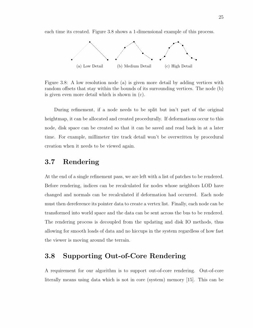
3.8 A low resolution node (a) is given more detail by adding vertices withrandom offsets that stay within the bounds of its surrounding vertices.The node (b) is given even more detail which is shown in (c). . . . . 25

4.1 High level flowchart of the implemented system. . . . . . . . . . . . . 41

4.2 Flowchart of the implemented algorithm. . . . . . . . . . . . . . . . . 42

4.3 Use case diagram for the system. . . . . . . . . . . . . . . . . . . . . 43

4.4 Terrain editor on a Hawaii data set. . . . . . . . . . . . . . . . . . . . 444.5 The buffer used to ensure data was available for deformation under-

neith the vehicle. . . . . . . . . . . . . . . . . . . . . . . . . . . . . . 444.6 Vehicle track deformation. . . . . . . . . . . . . . . . . . . . . . . . . 45

vi

List of Tables

4.1 Functional Requirements for the system. . . . . . . . . . . . . . . . . 32

4.2 Non-functional requirements for the system. . . . . . . . . . . . . . . 33

4.3 Structure of a Terrain (.ter) file. . . . . . . . . . . . . . . . . . . . . . 35

4.4 Structure of a Texture (.tex) file . . . . . . . . . . . . . . . . . . . . . 36

4.5 Pseudo code for multiple rendering passes using different frustums. . 37

1

Chapter 1

Introduction

Throughout the past decade, terrain rendering has been a highly researched area due

to the demand of military, scientific visualization, and computer gaming applications.

Even as the advances in graphics hardware continue to be released, these applica-

tions will always push the current technology to the limit such that a “brute force”

method will never be practical. Level-of-detail rendering algorithms are one of these

applications which continue to be developed to give the best visual representation of

large scale landscapes.

Terrain rendering commonly involves using a regular grid of evenly spaced height

values, referred to as a heightmap, which represents a terrain mesh in 2-dimensional

array. A heightmap contains a single channel that can be intepreted as an amount

of displacement of a surface. Using a heightmap allows for an easy representation of

the terrain mesh, but limits features such as overhangs and caves.

Terrain rendering comes with one major problem: Size. First, brute force ren-

dering is no longer an option when dealing with large datasets, so a level-of-detail

approach needs to be taken. Second, given a large heightmap, quite a bit of memory

can be taken up and thus out-of-core rendering needs to be supported.

Several algorithms acknowledge and address this terrain rendering problem. Pre-

viously published papers on this subject can usually be divided into two categories:

In-core dynamic level-of-detail rendering and out-of-core static level-of-detail render-

ing. When all terrain data resides in memory, updates to the height samples becomes

trivial; however, when dealing with out-of-core rendering, the notion of deformation

2

becomes less trivial. Therefore, a solution for out-of-core deformable terrain is needed.

This thesis presents an algorithm and its implementation which solves this problem.

The remainder of this thesis is structured as follows: Chapter 2 will present an

overview of the major existing level of detail algorithms. Each algorithm will be

evaluated on how applicable it is to our proposal. Chapter 3 presents a thorough

description of our solution. In Chapter 4 we will describe, in detail, our implementa-

tion of the algorithm and present the results obtained. Finally, we will conclude in

Chapter 5 and discuss any future work.

3

Chapter 2

Background

2.1 The Terrain Rendering Problem

There have been countless papers written on the terrain LOD algorithms and an

excellent survey of this subject which has 64 references is presented in a 2007 paper

by Pajarola [17]. The most common approach is to extract a good view-dependent

approximation of the mesh in real-time. This is done by storing data in a specific

hierarchical structure, in which a terrain can usually be categorized. Terrains can

be represented as a triangulated irregular mesh (TIN) [11], which gives the best

approximation, or a regular grid, which uses some-what more triangles to represent

a surface. They can be organized into quadtrees [19], binary triangle trees [7], or

directed acyclic graphs [13]. Refinement may take place on a per-triangle basis, or

tessellate aggregates of polygons. Some existing algorithms refine the terrain every

frame, having a “split-only” approach. Others may merge and split from previous

frame’s work. Refinement can be accomplished using a nested-error bound metric,

or, as in [14], solely the viewing position. Some terrains only support in-core, while

others out-of-core rendering and sometimes also provide the addition of procedural

detail on the fly.

In an ideal situation, a massive terrain with high amounts of detail, both sur-

rounding the viewer and stretching out to the horizon, composed of a single continuous

mesh, could be rendered. A brute force approach first comes to mind, but is quickly

limited by today’s graphics hardware. Even if we had the technology to render massive

4

amounts of data with one giant vertex list, applications would, instead of rendering

at say 1 meter detail resolution, demand centimeter or millimeter resolution. It is a

continuous cycle where the amount of realism, polygon count, and detail will never

be satisfied.

Modern video cards are built to render triangles - and lots of them. So why not

simply brute force the rendering process? Lets, for example, take a heightmap size

of 1024 × 1024. Rendering this heightmap would require roughly 2 million triangles

per frame. This isn’t too bad, but what if you wanted to visualize a heightmap

five orders of magnitude larger? This terrain data now consists of 100, 000× 100, 000

vertices. Given a brute force approach, we’re now looking at about 20 billion triangles

to be rendered, and assuming a 16- bit integer for each height value that is almost

20 gigabytes worth of data to be stored. Simply put, it’s impractical to render or

store this amount of data. With this in mind, the first problem of terrain rendering

immediately presents itself: Size. How is a large amount of terrain data stored and

how is it rendered in real-time?

Large scale terrain rendering is a well known problem across the computer graph-

ics community, and as a result, several “level of detail” algorithms have been devel-

oped and published. A level of detail (LOD) algorithm can determine which part

of the mesh to render with higher or lower detail, thus limiting the overall polygon

count of the mesh. The mesh that is usually closest to the viewer is rendered with

the highest amount of detail, while the mesh furthest away is rendered with less de-

tail. If the speed of rendering polygons is the bottleneck of the application, then any

simple LOD algorithm may suffice. However, with modern hardware able to render

huge amounts of triangles per frame, this usually isn’t the case. The bottleneck then

resides on the massive amount of data used to represent the terrain mesh. Therefore,

some of these LOD algorithms support out-of-core rendering, which allows terrain

data that exceeds system memory to be drawn.

Since terrain data can consume such a large memory footprint, out-of-core al-

gorithms often limit their datasets to be static (i.e. unchanging). Large amounts

5

of terrain data are usually processed in a way that leaves the geometry optimal for

video hardware and is not expected to change, ever. What if deforming the terrain in

real-time was a requirement? When dealing with an out-of-core terrain system that

handles dynamic updates of it’s height values, things aren’t so trivial. For the most

part, the areas of the mesh that need to be rendered stay in memory, while areas that

aren’t visible can be discarded to the hard-drive until needed. With a deformable

terrain, updates to the mesh could be made outside the viewing frustum, in which

case those areas would need to be loaded, updated, and cached back to disk. If a

hierarchy of LOD mesh representations were preprocessed, then updated data may

need to be propagated up through the tree or reprocessed altogether. The idea of

dealing with large amounts of data in a dynamic terrain algorithm can quickly become

mind-numbing, and thus, when combined with the first problem, a second problem

of terrain rendering is presented: Dynamic terrain. With an out-of-core terrain algo-

rithm in place, how can dynamic updates of the heightfield be applied and continued

to be rendered in real-time?

The rest of this chapter will present an overview of some of the major existing

terrain algorithms. Each algorithm will be evaluated on its applicability to a large

scale deformable terrain system, including level-of-detail rendering, out-of-core sup-

port, dynamic updates of the heightmap, and adding detail resolution in real-time.

2.2 Lindstrom 1

2.2.1 Overview

At Siggraph’96 Lindstrom et al. published the paper Real-Time, Continuous Level

of Detail Rendering of Height Fields [12]. In this paper they present a two step

algorithm that simplifies uniformly gridded terrain data (i.e. heightmap) to achieve

a continuous level of detail mesh. In their paper, they explain how their algorithm

reduces the overall number of polygons to be rendered, creates smooth transitions

between LOD changes, and allows for dynamic changes to the geometry mesh. Their

6

two step process is performed each frame - coarse-grained followed by fine-grained

simplification.

The underlying data must have its x, y dimensions in the form 2N +1, where N is

an integer greater or equal to 1. Starting with the full resolution mesh, 3× 3 regions

are made into blocks where vertices on the edge of a block share its vertex with its

neighbor. 2 × 2 blocks are then joined together and simplified by removing every

other row and column vertex. This new, simplified, block now covers the total area

as the original four smaller blocks but contains the same amount of vertices as a single

one. This process is continued recursively and each block is stored in a quadtree such

that the smallest, highest resolution blocks are the leaf nodes, and the largest, lowest

resolution block is the root node. Since doing a fine-grained (per vertex) simplification

would be too costly a procedure on the entire terrain, a coarse-grained simplification

process is performed which determines which block from the quadtree to use. A

maximum geometrical error, of all vertices in the block, is calculated and taken into

consideration during this step. Then, for each block, a fine-grained simplification is

used to simplify each block on a per-vertex level.

Fine-grained simplification is a retriangulation of each LOD block in which in-

dividual vertices are considered for removal. In this step, many smaller triangles can

be replaced with fewer, larger, triangles depending upon a specific geometrical error

tolerance. Two small adjacent triangles can be merged into a larger, single triangle.

The geometrical error is the change in slope between the adjacent triangles and the

larger triangle. Basically, a quantitative measure is calculated depending on how well

the larger triangle can represent the smaller two. As the geometrical error increases,

the chance for merging becomes smaller and smaller. The error is projected to screen

space and then determined if a merge should take place. This process is applied

recursively until no more vertices can be removed.

The authors also explains how vertex dependencies are used in the fine-grained

simplification step to make sure vertices are removed correctly. Within a block,

triangles can be organized in a binary tree, where the smallest triangles are the leaf

7

nodes and larger triangles correspond to a higher level. Vertices are to be considered

for removal in a bottom-up fashion. Vertex dependencies are required over block

boundaries since neighboring blocks may have a different level of detail.

2.2.2 Evaluation

The coarse-grained simplification process is extremely simple and is a great way to

quickly cut down on polygon count; however, the fine-grained simplification is too

CPU intensive, especially on large block sizes. It would be easy to create additional

detail by extending the quadtree at the leaf nodes, and updating the maximum error

could be done in real-time. Even though the authors suggests that changing the

terrain data is possible, the entire quadtree would have to be recreated and would be

too computationally expensive on large data sets. Also, this paper doesn’t suggest

any out-of-core implementation.

2.3 ROAM

2.3.1 Overview

ROAMing Terrain: Real-time Optimally Adapting Meshes [7], by Duchaineau et al.

is a well known level of detail algorithm. It is conceptually very close to Lindstrom’s

algorithm; however, instead of performing operations on individual vertices, ROAM

is strictly based on a binary triangle tree (bintree). Instead of dealing with a com-

plete terrain system that performs out-of-core paging for geometry and textures, and

selection of level-of-detail blocks, the authors focus on in-core geometry management.

Given a binary triangle tree, split and merge operations are performed using a dual

priority-queue system to achieve a level of detail representation of the underlying

data.

ROAM starts with a preprocessing step that produces a nested view-independent

error-bounds that works along side the bintree. When deciding to split or merge a

specific triangle in a bintree, the pre-computed error bound is taken into consideration

8

along with the view-dependent metric. The ROAM paper uses a metric based on

nested world-space bounds, where a world-space volume (called a “wedgie”) contains

the points of the triangle. World-space bounds are computed bottom-up, such that

a node’s error-bounds is the maximum of its children’s world-space bounds.

Data is stored in a binary triangle tree. Each node is an isosceles right triangle

where the largest least detailed triangle is the root node. Two children can be created

by splitting along an edge formed by a triangle’s apex and the center of its hypotenuse.

In a split-only ROAM implementation, this could be performed recursively top-down

until a desired level of detail is met. However, a dual priority queue optimization has

been added, that uses frame-to-frame coherence, to split and/or merge triangles from

the previous frame. In this way, ROAM execution time is limited by the number of

triangle changes per frame.

ROAM also realizes that neighboring triangles could be a different resolution,

either coarser or finer by one level. In this case, before a split is made, neighboring

triangles may be force-split to eliminate cracks or T-junctions in the mesh. This is

done recursively until the base neighbor is at the same resolution level i.e. a diamond

is created. Doing this recursive step ensures a single continuous mesh.

2.3.2 Evaluation

Top-down refinement of a terrain mesh is a very simple concept. Detail resolution

could be added easily be extending the leaf nodes of the binary triangle tree with

some adjustments to the nested error-bounds. The authors state that ROAM is

suitable for dynamic terrain since the preprocessing of error-bounds computation

is localized and fast. However, ROAM only handles data that can fit into system

memory. Reprocessing large amounts (more than can fit into memory) of terrain

data is still unacceptable, especially if many deformations are occurring and requiring

error-bounds to be recomputed every frame.

9

2.4 Lindstrom 2

2.4.1 Overview

In 2001, Lindstrom and Pascucci, published the paper Visualization of Large Terrains

Made Easy [13], an out-of-core view-dependent terrain algorithm. Top-down refine-

ment is performed on terrain data to produce a continuous mesh, where refinement,

frustum culling, and triangle stripping operations are accomplished in a single pass.

This algorithm was made with simplicity in mind, as opposed to other involved LOD

approaches.

Top-down refinement is based on longest edge bisection, and the authors go

on to explain that this is accomplished by bisecting a triangle’s hypotenuse. This

has already been illustrated in ROAM; however, instead of a binary triangle tree, a

directed acyclic graph (DAG) is used to represent the data. A directed edge in the

DAG is represented by a vertex, created at the hypotenuse, that is connected by its

apex vertex. Therefore all non-leaf vertices are connected to 4 children vertices, and

have 2 parents. Vertices on the edge of the terrain have 2 children and 1 parent.

During refinement, if a vertex is active, then all of its parents must be active as well.

Each node contains a vertex, world space error value, and a bounding sphere.

Error values are nested when the DAG is built, such that a parent node’s error value

is as large or larger than all of its children. Also a node’s bounding sphere is large

enough to contain all of its children’s spheres. During refinement a node’s world

space error is projected into screen coordinates and tested against a user specified

threshold. Since a single continuous mesh is created after refinement, this step can

be decoupled from the rendering process, allowing rendering to be done on a separate

thread.

An out-of-core system is supported, but whereas previous algorithms deal with

paging of precalculated rectangular tiles of varying resolution, the authors instead

propose to optimize the data layout both in-core and out-of-core and allow the oper-

ating system to handle paging of data. Data then must be stored in such a way as to

10

minimize paging events and data indexing must be efficient. An interleaved quadtree

layout and indexing scheme are then presented to satisfy both of these requirements.

2.4.2 Evaluation

This algorithm simplifies the refinement step by doing only top-down refinement (no

merging or simplification) of the mesh, and becomes a powerful feature when de-

coupled from the rendering process. Detail addition could be accomplished, but the

entire DAG would have to be recreated on the fly. Although this algorithm demon-

strates out-of-core support, the preprocessed data layout is optimized for refinement

around the viewer. If deformation were to occur far away from the frustum, the data

layout is of no use. This method also breaks down when adding detail resolution to

the mesh, since it would disrupt data coherency.

2.5 Geomipmapping

2.5.1 Overview

With advances in graphic hardware, it is now common to spend less work on the

CPU to find a “perfect” mesh and throw more triangles to the GPU, even if they

aren’t really needed. Since sometimes it is faster (and easier) to simply render a

triangle than determine if it should be culled, there is now a balance and compromise

between brute force and dynamic refinement algorithms. In 2000, De Boer wrote the

paper Fast Terrain Rendering Using Geometrical MipMapping [6], a new approach

that exploits graphics hardware instead of computing perfect tessellation on the CPU.

De Boer states that the goal is to send as many triangles to the hardware as it can

handle. Since terrain data can be represented as a 2-dimensional heightmap (as also

used in all previous algorithms), the analogy of texture mipmapping was used and

applied to geometry.

Geomipmapping makes use of a regular grid of evenly spaced height values, that

must have 2N + 1 samples on each side. A preprocessing step is performed that cuts

11

the terrain into blocks, called GeoMipmaps, also with 2N + 1 vertices on each side

i.e. a 257 × 257 regular grid may be divided into 16 × 16 blocks of 17 × 17 vertices.

Vertices on the edge are duplicated for each block. Each block is given a bounding

box and is suitable to be stored in a quadtree for quick frustum culling. Finally, for

each block, a series of mipmaps are created by simplifying the mesh which is done by

removing every other row and column vertex.

Each geomipmap level has a geometrical error associated with it. For every

vertex that was removed during simplification, a world space error is calculated as

the distance between the vertex and the line of the interpolated simplified mesh.

The maximum error of all vertices is assigned as the geometrical error to the block.

Then, when deciding which geomipmap to use, it is projected to screen pixel space

and compared to a user-defined threshold. When the current geometrical error is too

high, a higher detailed block is used, and vice versa.

After each geomipmap block has been chosen, there will be several neighboring

blocks that reside at a different level of detail. As such, cracks will appear between

these block since one patch holds more detail than the other. De Boer fixes this

problem by omitting vertices on the edge of a higher detailed block to identically

match its lower detailed neighbor.

Geomipmapping can also be used for out-of-core rendering. De Boer suggests

that only visible blocks or those near the camera need to be in memory. Others can

be discarded to the hard disk until needed.

2.5.2 Evaluation

Geomipmapping is extremely easy to understand, implement, and also exploits the

benefits of the graphics hardware. Adding detail would be trivial, by simply reversing

the simplification step described in the algorithm. Deformation could be supported,

but geomipmaps would have to be recreated and geometrical errors recalculated. Out-

of-core support could be extended by having blocks remain in memory that are not

only close to the viewer, but also recently deformed. The downside is that the number

12

of geomipmaps increases quadratically (N2) based on the size of the terrain; there-

fore, possibly resulting in slow computation and rendering. Overall, Geomipmapping

suggests some very good ideas for an out-of-core deformable terrain.

2.6 Chunked LOD

2.6.1 Overview

At Siggraph’02, Ulrich presented a hardware friendly algorithm based on the concept

of a chunked quadtree, which is described in the paper Rendering Massive Terrains

using Chunked Level of Detail Control [23]. This algorithm, also referred to as Chun-

ked LOD, is somewhat similar to Geomipmapping; however, it scales much better due

to the quadtree structure. There is often confusion of the differences between Chun-

ked LOD and Geomipmapping since the algorithms are so similar. Chunked LOD

exploits a quadtree data structure of mipmapped geometry. Therefore the number of

rendered nodes does not quadratically increase due to the size of the terrain.

A requirement of Chunked LOD is to have a view-dependent level of detail algo-

rithm that refines aggregates of polygons, instead of individual polygons. As Lind-

strom1, Lindstrom2, and ROAM all tessellate down to a single triangle, Chunked LOD

refines chunks of geometry that have been preprocessed using a view-independent

metric. Since chunks are stored in a quadtree, the root node is stored as a very low

polygon representation of the entire terrain. Every node can be split recursively into

four children, where each child represents a quadrant of the terrain of even higher

detail than its parent. Every node is referred to as a chunk, and can be rendered

independent of any other node in the quadtree. Having such a feature allows for easy

out-of-core support.

In order to create the chunked quadtree, a non-trivial preprocessing step must

first be performed. Given a large heightmap dataset, height samples are partitioned

into a quadtree and simplified based on the properties of the mesh and not the viewer.

This can be done using any per-triangle tessellation algorithm, such as Delaunay

13

triangulation or binary tree tessellation as illustrated in ROAM. Depending on the

depth of the chunk, more detail is given to the final mesh.

Each chunk holds a list of renderable vertices, a bounding volume, and a maxi-

mum geometrical error. Starting with the root node of the quadtree, nodes are culled

and recursively split based on the viewing position and its geometrical error. Neigh-

boring chunks at different levels of detail are addressed by creating a “skirt” of extra

geometry that eventually, with tweaks of texture coordinates, fills in the frame buffer

so no artifacts are noticed. Utilizing skirts keeps chunks independent of each other,

which makes out-of-core support trivial.

2.6.2 Evaluation

Chunked LOD brings some powerful ideas to the table. The chunked quadtree struc-

ture is one of the best known hardware friendly level of detail algorithms used since

it can be used for very large out-of-core terrain. Adding detail resolution would re-

quire extending the chunked quadtree, which could be easily done in a preprocessing

step. However, deformation isn’t so trivial. Chunked LOD expects its mesh to re-

main static, and if any height samples were changed, it would require reprocessing

all of the quadtree, which is unacceptable for a real-time deformation algorithm. The

scalability of Chunked LOD is amazing, but would require some changes to adapt to

the deformation requirement.

2.7 Geoclipmapping

2.7.1 Overview

Another hardware friendly algorithm was presented by Losasso and Hoppe, in Geom-

etry Clipmaps: Terrain Rendering Using Nested Regular Grids [14]. They introduce

geometry clipmaps (geoclipmaps), which caches in a set of nested regular grids, cen-

tered around the viewer, to represent a terrain heightmap. The vertex data is stored

completely on the graphics card and is updated as the viewport moves. Geoclipmaps

14

makes use of two new features: decompression and synthesis.

A heightmap is successively down-sampled, using a linear filter, into a mipmapped

pyramid each at a power of two resolution. Each level can be partitioned into block

sizes for optimal vertex caching, and can also be used for frustum culling. Updates

then cache in levels of the pyramid and incrementally update using toroidal access,

i.e. 2-dimensional wrap around using modulos operations on the x and y. Each vertex

holds (x, y, z, zc) coordinates, where zc is height value at the next coarser level in the

pyramid. Since detail is nested around the viewer, Geoclipmaps completely eliminate

tessellation based on the underlying geometry, and only uses the viewport as a metric.

Therefore, no matter how the terrain is being rendered, a set of nested regular grids

will surround the viewer to maintain a somewhat constant framerate.

Cracks will always appear on regions that transition from one level-of-detail to

another. This is handled by stitching adjacent levels together on the region boundary

using degenerate triangles.

Terrain synthesis is implemented by adding uncorrelated Gaussian noise to the

coarser pyramid level. When adding detail, the terrain is guaranteed to be the same

each time it is viewed, therefore detail addition must be spatially deterministic. This

is accomplished by creating a small (50 × 50) array of precomputed Gaussian noise

values and indexing them based on the vertex coordinates. This computation has not

yet been ported to the GPU and still resides on the CPU.

Geoclipmaps exploit heightmap coherency and uses compression on the series of

mipmaps created. This is done in a coarse-to-fine manner, where subsequent levels

of detail can be predicted from its parent through interpolary subdivision, and the

result is compressed in an image coder. Losasso and Hoppe stated that a 40 gigabyte

heightfield of the United States was compressed into 355 megabytes, which can easily

fit into memory.

2.7.2 Evaluation

Geoclipmapping presents some extremely appealing features such as GPU-based ren-

15

dering, terrain synthesis, and refinement criteria. Terrain compression is an excellent

feature, but still doesn’t fit the bill for an out-of-core rendering requirement, espe-

cially if only a small memory footprint is available. Implementing out-of-core support

shouldn’t be much of a problem - instead of only pulling data from memory to GPU,

add a system to read data from disk into memory. Detail addition presented here is

a clear choice for multi-resolution deformation, and being able to extend the original

geometry provides for a lot of potential. Updating height samples could be doable,

but tricky. Any deformation of a pyramid level would call for all of the coarser levels

to be updated as well. If this was done within view, it could still be done on the

GPU, but any deformation outside the viewing frustum would require CPU compu-

tation. Updating the heightmap may also interfere with the compression algorithm

used, causing even more CPU work. Overall, Geoclipmapping is a very powerful LOD

algorithm, but would require a lot of work to adapt real-time deformation.

2.8 Extended Algorithms and Related Work

Extensions to the algorithms just presented have been developed in order to fill in

some of the missing pieces that each have. He [10], extends the ROAM algorithm

that adds multi-resolution support. Their system DEXTER, dynamically extends the

geometry hierarchy only where necessary - usually the case of a small deformation

such as tire tracks. DEXTER supports real-time deformable terrain using ROAM,

but limits the implementation to be in-core. Lauritsen and Nielsen [15] have combined

Geomipmapping and Chunked LOD to create a chunked quadtree data structure that

is used for rendering large scale terrain with procedural detail additions. Out-of-core

rendering is supported, but their terrain is expected to remain static.

A very closely related piece of work is presented by Atlan and Garland [5]. Their

paper, Interactive Multiresolution Editing and Display of Large Terrains, preprocesses

a heightmap into a hierarchal wavelet quadtree data structure, and allows for real-

time updates to the terrain mesh. The wavelet structure supports lazy propogation

of any updated vertices, such that coefficients at a particular node only change when

16

it needs to be rendered. Rendering is also decoupled from the rest of the terrain

processes to allow for smooth updating of the terrain. Out-of-core support would

require calcuating heights from root node coefficients for every renderable node, every

frame, and thus is listed as future work.

2.9 Summary

We have presented a sample overview of the major algorithms that exist today, and

have evaluated them on their applicability to an out-of-core deformable terrain sys-

tem. The algorithms presented above can generally be split into two categories:

In-core dynamic terrain and out-of-core static terrain. If all terrain data can reside

in memory, updates to the underlying terrain mesh can be done simply by obtaining

an offset to a preallocated array of memory. [7], [12], and [10], all support dynamic

changes to the heightfield and are able to recalculate the nested error-bounds on the

fly since the entire terrain data is so small. Out-of-core algorithms, such as [15] and

[23], preprocesses its geometry and even though it can handle extremely large terrains,

any changes to the heightmap would be too computationally expensive to reprocess.

There is clearly a missing piece in the mass of available terrain algorithms. How can

one support terrain deformation while handling out-of-core rendering? In Chapter 3,

we present our proposal.

17

Chapter 3

Large Scale Deformable TerrainAlgorithm

3.1 Overview

In this chapter we present an out-of-core, level-of-detail algorithm that supports dy-

namic updates to the terrain mesh. Since terrain deformation is a key focus to this

algorithm, we provide a utility to update the heightmap at any desired resolution,

allowing huge craters or small tire tracks to be deformed in real-time. Sometimes

a small deformation is required beyond the resolution of the underlying heightmap.

In this case, real-time procedural detail can be added to the terrain down to a user

desired resolution. Any newly added data will be treated the same as the rest of the

terrain mesh, and will be able to be paged in and out from hard disk when needed,

to fully satisfy the out-of-core requirement.

We combine many appealing features of several of the algorithms discussed in

Chapter 2 into our implementation. [15] presents a level-of-detail algorithm that

combines the quadtree structure and detail addition properties of Chunked LOD [23]

and Geomipmapping [6] respectively. This combination is nearly identical to the

coarse-grained simplification process presented in [12]. We plan to use this data

structure and adapt it for support of terrain deformation. Previous deformation

methods propogate modifications through a hierarchal tree. This can be tedious and

slow especially if several deformations are happening each frame. In our method no

propagation is required after a deformation takes place.

18

3.2 Limitations

Our proposed algorithm does have a few limitations. The terrain data needs to be a

heightmap, an evenly distributed grid of height samples, which limits features such

as caves or overhangs. Also, the dimensions of the data are required to be square

consisting of 2N + 1 data points on each side. This is a common requirement for any

level of detail terrain algorithm, and knowing this information ahead of time allows

for many optimizations. A one-time preprocessing step is required which, with large

datasets, can take a long time to complete.

3.3 Hierarchical Representation

At the core of our algorithm, a nested quadtree structure is used to organize the terrain

data such that each node has either four children or zero children. Likewise, every

node has a single parent, except for the root node. As in previous algorithms, the root

node defines a low-detail representation of the entire mesh, and each subsequent child

contains more detail at the scale of one quarter of its parents mesh. The amount of

detail at leaf nodes are equivalent to the resolution of the underlying heightmap. Each

node is therefore a regular grid of evenly spaced height values of varying resolution.

The quadtree is constructed using a simplification process similar to [12]. Starting

at the bottom, leaf nodes are partitioned into user-defined square dimensions. Each

node can be looked at as a reduced-size copy of the entire terrain and thus fulfills the

2N+1 square dimension requirement allowing edges to overlap by one vertex. Nodes

are combined into 2 × 2 partitions and up-sampled even further by removing every

other row and column vertex. This is repeated recursively until no more 2× 2 blocks

can be made. Each node is given a bounding box that encapsulates the entire mesh.

This is shown in Figure 3.1.

Using this simplification algorithm, a certain property can be seen through the

child-parent relationship within a quadtree. Given that a node has a parent; its data

can be made up of a portion of its parent’s data along with its own individual data.

19

(a) Original Heightmap (b) Partitioned into Seg-ments

(c) Merged and Simplified

Figure 3.1: The node simplification process to create a quadtree.

Figure 3.2 shows this property.

(a) Parent Node (b) Children Nodes

Figure 3.2: A parent node (a) with its vertices represented as white circles. Itschildren (b) are made up of a part of the parent data along with individual datashown as x’s.

Exploiting this property allows us to organize the node data in such a way that

no propagation is needed during deformation. Each quad node now separates its

individual data and points to the section of its parents data in order to create the full

grid of height values. In order to guarantee this property holds true, when a node

is loaded into memory, all of its ancestors must be in memory as well. This is not

hard to satisfy since every node in the quadtree uses the same amount of vertices to

represent its mesh. The memory layout for any given node is shown in Figure 3.3.

For example, the bottom left vertex of underlying heightfield belongs to the root

node. Children nodes simply receive a pointer to this vertex in order to access it.

This appears similiar to a wavelet compression scheme as shown in [5]; however, we

do not encode the children data within the parent’s node. Instead the individual

20

(a) Node Data

(b) Memory Layout

Figure 3.3: Node data shown in (a) is represented in memory as shown in (b).

raw data per node is stored in a file that can be loaded on demand. This eliminates

the need to decode node information at runtime and allows for deformation without

encoding new vertices into the quadtree. In order to query a nodes data, it must

simply dereference the vertices it points to.

3.4 Top-down Refinement

The goal of any terrain rendering algorithm is to quickly create the best approximation

mesh for each frame. Our approach uses a “split-only” top-down refinement that

traverses the quadtree from the root node for each frame. Bounding boxes are culled

against the current view frustum which can quickly discard large portions of geometry.

21

Previous algorithms refine their mesh based on properties of the underlying geometry,

using nested error-bounds. However, modifications to the heightfield would require

recalculation and propagation up the tree. We take an approach like [14] and limit

our refinement to be solely based on the viewer’s position. Obviously this approach

would look awkward if steep mountains jutted out of the ground with few vertices to

represent its peak. However, natural terrains are well suited since a smooth gradient

of vertices usually makeup the elevation data, i.e. a mountain peak doesn’t consist

of a single vertex.

For every node, the center of its bounding box is tested against the position of

the viewer. If it’s closer than some defined threshold the node is split into its four

children, else it is prepared for rendering. This process continues until there are no

more nodes to split. Ideally, a threshold should be used such that a nested regular

grid surrounds the viewer. Since no other metrics are taken into account during

refinement, this will give the best visual fidelity. Note that the LOD of a neighboring

node is never limited in any way, i.e. we do not implement a restricted quadtree or

enforce splitting of neighboring nodes [18]. Figure 3.4 and Figure 3.5 show a nested

regular grid and bounding boxes of a hierarchy, respectively.

Figure 3.4: A nested regular grid of a flat heightmap.

22

Figure 3.5: A quadtree displaying the bounding boxes of each node. Bounding boxesare culled against the viewing frustum to quickly elimate nodes during refinement.

3.5 Neighboring Nodes

3.5.1 Linking Adjacent Patches

Neighboring nodes play an important role in the overall scheme of terrain rendering,

and care must be taken in order to render smooth transitions between nodes of differ-

ent detail. It is common to see ugly seams between two patches at different levels of

detail, which is caused by gaps or cracks, or incorrect normal calculations for lighting.

Also, since each neighbor holds its own copy of edge vertices, care must be taken to

deform edges or across edge boundaries. Since quadtree refinement isn’t restricted, a

node’s neighbor may be a difference of zero, or one, or five, etc. In order to deal with

the variety of seam problems, nodes must be aware of their neighbors. Since a node’s

LOD may change frame by frame, neighboring links are recreated during refinement.

When linking nodes together, nodes must satisfy a strict rule: A node is only

allowed to point to a neighbor that is of equal LOD or higher (coarser). i.e. nodes can

only point to adjacent nodes on the same level of the quadtree or above. Figure 3.6

illustrates this idea further.

The most common way to refine a mesh is via depth-first traversal of the quadtree.

23

Figure 3.6: A node is only allowed to point to a neighbor that is of equal level ofdetail or higher.

However, in this way, neighboring nodes won’t be linked together correctly. Instead

a breadth-first traversal must be done during refinement. Whenever children nodes

are created, their parent is responsible for linking them to the rest of the quadtree.

3.5.2 Cracks

Now that nodes are linked together during traversal, gaps or cracks that appear on

the seams of dissimiliar LOD’s may be properly stitched together. Stitching is done

by having the finer detail node omit vertices on its edge to match that of its coarser

neighbor. This is done by rendering degenerate triangles in which the graphics driver

will recognize and discard. Note, the use of geometrical skirts [23] was not chosen.

The size of the skirt may change after any deformation to the vertices, and the

recalculation can become tedious and slow. Figure 3.7 illustrates the removal of

T-junctions by utilizing degenerate triangles.

(a) T-Junction (b) Degenerate Triangles

Figure 3.7: T-Junctions appear at the neighboring nodes of different levels of detail.Omitting vertices via degenerate triangles removes any possible cracks from the mesh.

24

3.5.3 Normal Calculation

Neighbor links also play an important role for correct normal calculation. Normals

are needed to simulate a realistic lighting model and can also be used for collision

response or terrain following. The biggest problem of normal calculation once again

presents itself on the seams of terrain patches. Vertices on an edge need the height

values of neighboring nodes.

The most common approach to calculate a normal is to compute a normal for

each vertex in the heightfield by taking the average normal of all faces that contain the

vertex [24]. This process usually consists of several costly mathematical operations,

such as square roots. However, by exploiting properties of the heightfield several

optimizations can be made. The method we use is described in [22], which only

requires the four neighboring heightsamples of a vertex. In order to create a smooth

transition across a patch seam, neighboring vertices must be queried. The computed

normal is then stored for each edge. Using a breadth-first traversal, once again

guarantees that higher detail nodes will be computed after coarser nodes, overwriting

any previous calculation.

3.6 Detail Addition

In order to save disk space, real-time procedural detail can be created for the original

terrain resolution. This is done by extending the quadtree down to a user specified

level in real-time. As we simplified the quadtree bottom-up in to initially to create

the quadtree, a reverse and opposite process can be used to extend detail into the

leaf nodes. This is done by adding rows and columns into each node and linking it

properly with its parent node. In order to create somewhat non-uniform detail, linear

interpolation won’t suffice. Instead, fractals are used, specifically a midpoint dis-

placement algorithm to create detail. For each interpolated vertex, it can be shifted a

random amount such that it stays within bounds of its surrounding vertices. Since de-

tail addition is so subtle, it does not need to be deterministic thus can be randomized

25

each time its created. Figure 3.8 shows a 1-dimensional example of this process.

(a) Low Detail (b) Medium Detail (c) High Detail

Figure 3.8: A low resolution node (a) is given more detail by adding vertices withrandom offsets that stay within the bounds of its surrounding vertices. The node (b)is given even more detail which is shown in (c).

During refinement, if a node needs to be split but isn’t part of the original

heightmap, it can be allocated and created procedurally. If deformations occur to this

node, disk space can be created so that it can be saved and read back in at a later

time. For example, millimeter tire track detail won’t be overwritten by procedural

creation when it needs to be viewed again.

3.7 Rendering

At the end of a single refinement pass, we are left with a list of patches to be rendered.

Before rendering, indices can be recalculated for nodes whose neighbors LOD have

changed and normals can be recalculated if deformation had occurred. Each node

must then dereference its pointer data to create a vertex list. Finally, each node can be

transformed into world space and the data can be sent across the bus to be rendered.

The rendering process is decoupled from the updating and disk IO methods, thus

allowing for smooth loads of data and no hiccups in the system regardless of how fast

the viewer is moving around the terrain.

3.8 Supporting Out-of-Core Rendering

A requirement for our algorithm is to support out-of-core rendering. Out-of-core

literally means using data which is not in core (system) memory [15]. This can be

26

accomplished by discarding patches to the hard-drive that are not needed and keeping

recently viewed and deformed patches in memory.

3.8.1 Loading and Caching Data

At any given time during the refinement process, a patch may need to be split, yet

its children are not in memory. In order to support out-of-core rendering, a separate

loading and caching thread is spawned that works alongside the main process. This

thread is constantly being fed patches to either load or write to disk. If for any reason

a patch cannot be split because its children haven’t been loaded yet, refinement at

that patch will stop and it will be selected for rendering. In this way the system will

never halt or hiccup while waiting for data to be loaded off of disk - it can render the

parent node until all children have finished loading.

It is not always easy to tell which patches will be needed at any given time; there-

fore, a least recently used (LRU) algorithm is used to determine which ones to keep

in system memory. Maintenance is performed when a user defined memory footprint

is reached. Once over quota, maintenance will remove patches until a desired quota

is met This is done by keeping a timestamp on each node. If a node is ever rendered,

or in our case deformed, the time stamp can be updated. Cache maintenance will

use a priority queue to sort the nodes based on the last time they were accessed and

add them to a load/cache thread. It is important to only consider nodes that are

currently leafs for caching, since every node points to its parent for some of its data.

We wouldn’t want the root node, for example, to be removed because the viewer

hadn’t viewed the terrain from the furthest distance.

3.8.2 Memory Management

Utilizing a small data set means that the quadtree could be completely full. At

run-time the system could allocate memory to every single node to where it could

stay in memory until the program was terminated. Out-of-core rendering makes this

approach obsolete. Depending on the actions of the user (fast movement or several

27

deformations) and the memory footprint, nodes may require constant allocation and

deallocation. Instead of using operators such as new or delete which are notoriously

slow for small frequent allocations another approach is taken. [9] describes a freelist

to achieve fast allocation and dellocation without the penalties of memory fragmen-

tation. In its most basic state, a freelist is a preallocated pool of memory in which

the system can pull from and release to without inducing the overhead of the default

memory manager.

Its important to keep a freelist and memory footprint integrated. Running out of

nodes from the memory pool, yet still under the quota limit, could lead to unexected

results.

3.9 Deformation

The entire algorithm leads up to terrain deformation. Assuming many deformations

taking place at once, propagation of nested-error bound or vertex data would become

tedious and slow. Instead the algorithm presented so far has adapted itself to deal

with this sort of action. Deforming at a high resolution will end up modifying ancestor

nodes due to the child-parent relationship. Refinement is based on view position alone

and thus eliminates the need for nested error-bounds. A separate memory manager

is implemented to keep recently used nodes (rendered or modified) in memory. Detail

addition has been discussed to extend the quadtree, allowing for deformations smaller

than the original terrain resolution to take place.

3.9.1 Selection Brushes

In order to deform a section of terrain, a specified area must be selected. We call

this a brush. Brushes define a 2-dimensional rectangular region over the terrain that

consists of a position, width, height, and resolution. Brushes consist of an array of

pointers that point to specific vertices in the terrain. This allows for deformations

to take place across node boundaries. Once a brush has been created, nodes that

intersect the brush are picked out during refinement, and the correct vertices of each

28

are given to the brush. By dereferencing the brush we gain access to the vertex

data which can be overwritten with new data. Since vertices on edges are duplicated

for each patch, care must be taken for deformations across boundaries by syncing

adjacent vertices. This is done in a pre-rendering step that compares dirty flags of

neighboring nodes in the quadtree.

Refinement of the quadtree was discussed previously with regards to the viewing

position only. Many, if not all, refinement algorithms cull nodes and discard data

if they aren’t being seen by the viewer. In our implementation this can’t be the

case, Refinement is based not only on the viewer position, but brush positions as

well. During refinement a node may not be in the viewing frustum, but still selected

for deformation. In this case, the same low-resolution patches can still be selected

for rendering, but refinement must continue in order to load in data for selection

brushes. Once all of the data has been loaded into memory, deformation may occur

on the selected brush. Therefore, the viewer may be looking down upon the terrain at

a high elevation, and even though a low-polygon mesh is being rendered, refinement

may continue to load and keep data deep in the quadtree in system memory.

3.9.2 Procedural Data

Deformation can take place at a varying resolution, from the root node to highest

detail. When a node is chosen for rendering, it is possible that an ancestor has previ-

ously been deformed. Time stamps can be compared, and if a nodes last modification

is less than its parents, it needs to adapt its data to the parent mesh. This is done

by creating procedural data, exactly as performed in the detail addition step of the

algorithm.

3.10 Textures

In actuallity, the number of polygons in a terrain mesh doesn’t add as much detail or

realism as one might think. A highly detailed texture can be layed over a low polygon

mesh and everything usually looks just fine. If a low quality texture is used over a high

29

polygon terrain, the overall quality is usually limited to the quality of the texture.

In Section 3.8 we explained the necessesity of a caching system in order to handle

very large terrain datasets. One can assume that along with a large heightmap, a

large texture is needed as well. For example, it is common for digital elevation maps

(DEMs) to come with extremely large satellite images usually even larger in size than

the original height data.

3.10.1 Texture Quadtree

Textures can be dealt with much like our terrain geometry. A large texture can be

cut into user defined partitions, starting at the highest detail, and merged into 2x2

blocks before being mipmapped. This process continues until an entire quadtree is

built. The root node will then hold the lowest resolution image, and the leaf nodes

will hold the highest resolution image.

A quadtree typically lends itself to mapping its nodes to a node in the texture

quadtree. However, depending on the size of the extended quadtree (detail included),

it could become impractical to create a texture quadtree of the same depth. Thus

it is common to have a much shorter quadtree of textures. If a node in the terrain

quadtree can’t be mapped directly to a node in the texture quadtree, due to it being

too deep, it can use its parent’s texture and adjust its texture coordinates accordingly.

Therefore, nodes are responsible for a specific texture node. When a node is being

loaded or deleted it can also load or delete its texture.

3.10.2 Seams

Textures come with unwanted seams on the boundaries of patches at different levels of

detail, due to the texture filtering being used. If you can tolerate “nearest” filtering,

then the results will be perfect since no blending of adjacent pixels will take place;

however, “linear” filtering is usually desired. Seams will then appear at the texture

edges because the edge texels are not being blended with the correct neighbor texel.

This can be solved by overlapping adjacent textures when the texture quadtree

30

is created, so that neighboring texture have the exact texels on their corresponding

edges. Clamping the texture edges will cause edge texels to blend with itself, removing

the seam. Since there is no pefect solution, the amount of pixels to overlap can vary.

3.11 Summary

In this chapter we have presented our terrain algorithm. It is an algorithm capable of

out-of-core rendering, real-time deformation, and real-time procedural detail creation,

while handling large textures and large scenes.

The level of detail algorithm is based on a chunked quadtree structure that

exploits the properties of a child-parent relationship. Refinement is based on camera

position alone, and results in no propagation of data once a deformation occurs.

Deformation is done by creating a brush that points to specific vertex data across

one or several patches, and can occur as very high resolutions by procedurally adding

detail to the mesh. Any added detail that is deformed is given an offset to disk so

that it becomes a permanent piece of the terrain.

31

Chapter 4

Implementation

4.1 Overview

This chapter presents the implementation and results of our algorithm. This algo-

rithm was made into a library and provides an interface that is intended to be open

ended and easy to use in existing projects.

It was developed using the C++ programming language and used OpenGL to

utilize the graphics hardware. The library is crossplatform, having minor preprocessor

differences for Windows and Linux versions. We used the GDAL library [2] to convert

DEM (.dem) files into binary terrain (.bt) format which the library was made to read.

Information about the binary terrain format can be found at [3]. GDAL was also used

to read the texture image which is needed to create the texture quadtree. Figure 4.1

shows a high level flowchart of the implemented system. Figure 4.2 shows a lower

level flowchart of the algorithm.

4.2 Library API

An interface was created to provide complete access to the major utility of our algo-

rithm, with hope of hiding some of the unwanted detail. This can be seen through a

list of functional and non-fuctional requirements, along with a use case diagram.

32

4.2.1 Functional Requirements

Functional requirements are perceived as the overall behavior of the system. They

include input, output, data manipulation and processing, and other specific function-

ality. These were conceived with the ideas of ease of use, and flexibility. We want

to expose a lot of functionality to the user so that the library can fit into several

different applications. Table 4.1 shows the system’s functional requirements.

F01 The system shall display a level of detail representation of the terrain mesh.F02 The system shall allow fly-by movement around the scene.F03 The system shall allow the user to select an arbitrary area for deformation.F04 The system shall allow the user to change the resolution of the selected area.F05 The system shall allow the user to choose a desired resolution of the terrain.F06 The system shall allow the user to choose the size of a terrain patch (in vertices).F07 The system shall allow the user to choose a maximum memory quota.F08 The system shall allow the user to choose a desired memory quota.F09 The system shall allow the user to choose a segment size.F10 The system shall allow the user to choose a texture size.F11 The system shall allow the user to choose a height scale.F12 The system shall allow the user to choose a maximum brush size.F13 The system shall allow the user to preprocess terrain data.F14 The system shall allow the user to preprocess texture data.F15 The system shall allow the user to load terrain data.F16 The system shall allow the user to load texture data.F17 The system shall allow the user to toggle wireframe/fill mode.F18 The system shall allow the user to toggle textures on and off.F19 The system shall allow the user to toggle fog on and off.

Table 4.1: Functional Requirements for the system.

4.2.2 Non-functional Requirements

Non-functional requirement are contrasted with functional requirements and specify

criteria that allows the system to be judged. These show the major features supported

and the constraints of the system. Table 4.2 shows the system’s non-functional re-

quirements.

33

N01 The system shall use the C++ programming language.N01 The system shall use the OpenGL graphics library.N03 The system shall use the GDAL library.N04 The system shall remain independent of operating system.N05 The system shall remain independent from any specific windowing toolkit.N06 The system shall decouple rendering, updating, and disk IO.N06 The system shall use digital elevation data in Binary Terrain (.bt) format.N07 The system shall use terrain data with dimensions 2N + 1× 2N + 1.N08 The system shall allow for real-time deformation of terrain data.N09 The system shall allow for muli-resolution deformation.N010 The system shall allow for real-time procedural detail generation of terrain.N011 The system shall allow for large textures to be used.N012 The system shall use textures with dimesions 2N × 2N .N013 The system shall allow for out-of-core rendering.N014 The system shall write any procedural data to disk if its been altered.

Table 4.2: Non-functional requirements for the system.

4.2.3 Use Case Diagram

The functionality shown through to the user in the end is displayed through a use case

diagram, which is developed through functional requirements. Only major fuctional

requirements are shown through to the user. There is only ever one actor interacting

with our system at one time which is the user running the application. Figure 4.3

shows the use case diagram.

4.3 Preprocessor

4.3.1 Overview

The first step to using the system is to preprocess terrain and texture data. This

results in a terrain data file (.ter) and a texture file (.tex) that the system can read

back in at any time. Preprocessing may take a while, but only needs to be done

once per data set. The resulting files are usually very big since no compression was

implemented. The texture files also duplicate a lot of data when creating a quadtree.

34

4.3.2 Terrain File

Terrain data is built as explained in Section 3.3. Data was recursively processed into

a quadtree by seeking to specific offsets in the binary terrain file. Information such as

world coordinate, level of detail, children file offsets, and several other flags are written

as a header before writing the raw heightmap data. The .ter file contains a header

with basic information about the terrain followed by every node in the preprocessed

quadtree. The header holds the offset to the root node in the file, and every node

holds the offsets to its children nodes. Table 4.3 shows the file structure of a .ter file.

4.3.3 Texture File

Texture data was read in using the GDAL library, which supports a variety of file

formats. Our textures were supplied in jpeg format. A texture quadtree was created

by recursively reading in scanlines provided by GDAL. With any scanline, bits of an

image can be used to mipmap the texture. In our implementation we used nearest

sampling when upsampling texture data. In order to avoid seams, an overlap of one

texel was chosen and averaged together with the original value. Therefore the edges

of adjacent texture nodes share the same value. The texture file uses much of the

same format as the terrain file which is shown in Table 4.4.

4.4 Brush Selection

The user is able to select a region on the terrain to create a brush. Once its created,

they have the option of increasing or decreasing its resolution. Patches are forced to

be split to at least the resolution of the brush if they intersect the brush boundaries.

Brushes are rendered as a seperate polygon slightly offsetting the terrain mesh. A

maximum brush size has been implemented to keep users from selecting too much

terrain, and possibly overloading the system with too many triangles needing to be

rendered.

35

Bytes Contents Description4 (int) header Terrain header tag4 (int) map size Size of the map4 (int) file depth Quadtree depth based upon file

resolution4 (int) tree depth Extended quadtree depth based

upon the desired resolution4 (int) root offset file offset of the root node infor-

mation

4 (int) worldX Node x position in world coordi-nates

4 (int) worldZ Node z position in world coordi-nates

4 (int) world stride The stride inbetween vertices ofthe node

4 (int) size Size of the patch in coordinatespace

4 (int) bytes Size of the patch in bytes4 (int) LOD Number representing the resolu-

tion (level of detail) of the node8 (int) last update timestamp for the last time the

node was deformed1 (bool) leaf node Flag telling if the node is cur-

rently a leaf node in the full ex-tended quadtree

1 (bool) file leaf node Flag telling if the node is a leafnode in the file quadtree

1 (bool) top dirty edge Flag telling if the top edge is dirty(used for syncing edges)

1 (bool) bottom dirty edge Flag telling if the bottom edge isdirty (used for syncing edges)

1 (bool) left dirty edge Flag telling if the left edge is dirty(used for syncing edges)

1 (bool) right dirty edge Flag telling if the right edge isdirty (used for syncing edges)

4 (int) top left child offset Offset of a node’s top left child4 (int) top right child offset Offset of a node’s top right child4 (int) bottom left child offset Offset of a node’s bottom left

child4 (int) bottom right child offset Offset of a node’s bottom right

childsize*size*4 bytes data Raw heightmap data for this node

Table 4.3: Structure of a Terrain (.ter) file.

36

Bytes Contents Description4 (int) header Texture header tag4 (int) image size Size of the textures per node8 (int64) root offset File offset for the root node

4 (int) worldX Texture Node x position in worldcoordinates

4 (int) worldZ Texture Node z position in worldcoordinates

4 (int) LoD Number representing the resolu-tion (level of detail) of the node

image size * image size * 3 data Raw image data (3 channel)

Table 4.4: Structure of a Texture (.tex) file

4.5 Supporting Large Scenes

Extending terrain detail causes the terrain as a whole to be resized to a different

resolution. Instead of having a 1-meter resolution map, detail can be added so now

its a 1-millimeter map. In order to properly represent detail, the entire terrain needs

to be increased in scale.

4.5.1 Floating Point Precision

As worlds get substantially bigger, the amount of precision to reprensent world coor-

dinates gets smaller and smaller. For example, if units represent meters and our world

is 100km square, at the farther corner of the world a 32-bit number will allow us to

represent 7.8mm granularity [8]. The larger the world coordinates, the less accurate

they will be at the farthest extent. Therefore floats usually have to be converted

to doubles since there are not enough bits to represent a large number with high

precision.

Unfortunately the graphics hardware only performs floating point operations,

so precision is lost during operations such as matrix transformations. Traveling to

the farthest extent of your terrain will result in seams between patches or jittering

movement when the camera moves. It is best to partition the world into a user defined

segment space, where each node belongs to a segment and is given an offset.

37

Instead of transforming the camera and translating patches during rendering,

thus losing precision, transforms can be made in segment space, such that the world

now revolves around the camera within a segment. This will solve any and all accuracy

problems that large scenes come with. Unfortunately, this doesn’t come without a

burden. If this method is used, then all objects need to be represented in segment

space which can prove difficult, especially when using a scenegraph.

4.5.2 Depth Buffer Precision

Along with large world coordinates, precision is also an issue with the depth buffer.

Ideally the user will want to see detail an inch from his nose while also seeing the moon

in the sky. Unfortunately a 24 or 32-bit depth buffer can’t support such a task. Since

the depth buffer is not linear, there are many more bits allocated to the precision of

objects closer to the camera than further. Precision is gained exponentially as you

push out the near clipping plane. However, in our terrain we will sometimes want to

view millimeter resolution, without culling the mountiains in the horizon.

Several methods can fix this problem, such as using imposters [16], or a multi-

pass rendering system that renders the scene in sections, clearing the depth buffer

while altering the frustum each time. In our implementation we allow for multiple

rendering passes. Table 4.5 shows the steps required to perform such a task.

1. Set zFar to the maximum value needed.2. Set zNear = zFar / ratio.3. Clear z-buffer.4. Render scene and cull to the adjusted frustum.5. Set zFar = zNear.6. If zNear isn’t close enough yet go back to step 2.

Table 4.5: Pseudo code for multiple rendering passes using different frustums.

4.6 Use Case Scenarios

Two sample applications were developed utilizing this library. The first has a simple

fly-by mode which allows the user to select arbitrary sections of the terrain via a mouse

38

pointer, and allowing the user to add or remove resolution of the selected brush. A

hill algorithm was implemented to create simple hills or craters in the terrain, once a

brush was selected. This application shows off the basic usage of the terrain library.

The second application involved using the Bullet Physics Library [1] which placed a

wheeled vehicle on the terrain to drive around. This application allows the user to

drive the vehicle and shows off very small deformations with tire tracks.

4.6.1 Terrain Editor

In its most basic form, this library can be expressed as a terrain editor. The data used

for this demo was obtained from [3], which holds 10-meter elevation data of the big

island of Hawaii along with a 4096× 4096 texture. The terrain file has dimensions of

8193×8193 and was already in binary terrain (.bt) format. It was first converted into

the internal .ter file and the texture image (.jpg) was converted into a .tex file. Since

these files were so small, the preprocessing took less than five minutes. The desired

size of the terrain was increased to 134217729×134217729 which gives approximately

half-millimeter resolution. Since the terrain is so big (a single OpenGL unit represents

.6 millimeters), two rendering passes were made to help with depth buffer precision.

On the first rendering pass, the far clipping plane was set to 130,000,000 and the near

clipping plane was set to 1,500. On the second rendering pass, the far clipping plane

was set to 1500 and the near clipping plane to 1. With this demo, the user is able to

move around the scene via keyboard and mouse input. By clicking and dragging the

mouse, the user can select a single axis-aligned brush, and change the resolution of

that brush via keyboard input. Once a brush is selected with the desired resolution,

the user may create a hill or crater by raising or lowering the terrain via keyboard

input. Any changes to the terrain are automatically saved to the .ter file and will be

loaded back in when the application restarts. Figure 4.4 shows screen shots of this

demo.

39

4.6.2 Tire Track Deformation

The goal of this demo was to show small tire track deformations of a wheeled vehicle.

A 10-meter DEM (.dem) was used along with a huge 1-meter texture image in .jpeg

format. Unfortunately, these data files did not come in the required dimensions and

therefore were processed through a separate application to pad the data with “no

value” values to the closest 2N +1 and 2N dimensions. As a result, the elevation data

was padded to a 4093 × 4093 dimension and texture data padded to 32769 × 32768

dimension. The elevation data was then converted into binary terrain (.bt) format and

both data files were then preprocessed through the terrain library into their respective

.ter and .tex files. The desired resolution of the terrain was set to 2097153× 2097153

which results in about 2-centimeter resolution, and sets its patch size to 17×17. The

texture was processed into a quadtree using 128×128 texture chunks. The processing

for the .ter file took about 5 minutes, where the .tex file took over 25 hours.

The application was built using the Bullet Physics Library, which the original

4093 × 4093 10-meter dem was used as the underlying collision mesh. Bullet also

registered a single vehicle as a rigid body. The underlying terrain collision mesh was

slightly lowered to simluate the wheels sinking into the ground. All of the added

resolution from 10-meter down to 2-centimeter was considered soft soil, which the

vehicle would not collide. Since the application was only meant to display dynamic

deformation of tire tracks, the physics collision mesh remained static.

Deformation was performed by selecting a 25× 25 brush benieth the tires of the

vehicle and the resoution of the brush was allowed to change via user input. In order

to ensure that patches at the desired level of detail were available for deformation,

a “brush-buffer” surrounded the tank to force disk reads if necessary. Figure 4.5

illustrates the brush buffer.

The vehicle is able to drive around the terrain and deform a set of tire tracks

using keyboard input. Note that this application does not demonstrate a physical

model for soft soil deformation. [4] and [20] discuss a more realistic model. Figure 4.6

40

shows a series of screen shots for this demo.

41

Figure 4.1: High level flowchart of the implemented system.

42

Figure 4.2: Flowchart of the implemented algorithm.

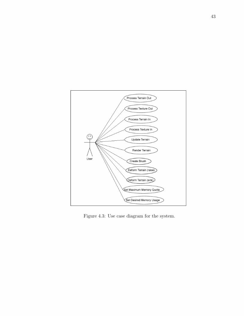
43

Figure 4.3: Use case diagram for the system.

44

Figure 4.4: Terrain editor on a Hawaii data set.

Figure 4.5: The buffer used to ensure data was available for deformation underneiththe vehicle.

45

Figure 4.6: Vehicle track deformation.

46

Chapter 5

Conclusion and Future Work

5.1 Conclusion

We have presented a complete level-of-detail terrain algorithm including the major

features of deformation and out-of-core rendering. To our knowledge, this is the first

out-of-core deformable terrain algorithm. The overall goal is to allow a simulation of

many entities modifying and deforming a massive (out-of-core) terrain, regardless of

the viewer’s position. Refinement is not only based upon the viewing frustum, but

also takes into account the selected deformation brushes. This allows data that is not

being viewed to remain in memory and be subject to deformation. Previous methods

that allow out-of-core rendering usually preprocess the geometry into a triangulated

irregular mesh for optimal polygon throughput, and require that the terrain mesh re-

main static. Other, in-core, algorithms support changes to the underlying heightmap,

but need to recalculate and propagate nested error-bounds through a hierarchal struc-

ture. Our approach eliminates the need for any geometry tessellation or propagation

after a modification to the terrain heightmap. By exploiting the features of a regular

grid, x and z coordinates will never change requiring only updates to the y coordi-

nate (height offset). The quadtree structure exploits a child-parent relationship in

which child nodes actually point to their parent’s data. In this way, when the data

of children nodes are modified, the pointer actually dereferences some parent data

completely eliminating any propagation back up through the quadtree. The need for

nested error-bounds is also eliminated by depending solely on the view position for

47

refinement. Even though this results in a less accurate refinement, the tessellation is

tolerable and the tradeoff of propagation removal is well worth it.

Deformation is allowed to be done at any resolution within the extended quadtree.

The quadtree may be extended to a user specified resolution by scaling up the original

terrain and adding procedural fractal detail to the leaf nodes. These extra nodes are

created on the fly in real-time and only need to be saved to disk if deformed. Since

detail addition is so subtle, the extra nodes do not need to be spatially deterministic

and can be randomly created each time. By comparing the time stamp of a node’s

parent, data may procedurally adapt to a low resolution modification using this same

method to create detail.

Along with our algorithm, we have presented support for large texture maps,

fast normal calculation, and dealing with large world coordinate and depth buffer

precision.

5.2 Future Work

For simplicity, not all optimizations were used when implementing this algorithm.

It would be possible, with some effort, to port the entire algorithm to the GPU.

Terrain data would reside completely in video memory in the form of a texture, and a

quadtree structure could be mimicked via indices to a memory location. Vertex lists

can easily be generated due to the regular grid layout, and indices could properly be

generated with triangles in a vertex shader.

Creating disk space for nodes of added detail disrupts data coherency when layed

out on disk. Though this isn’t seen as a huge problem, it could be looked into further.

Currently the algorithm only allows for a single brush to be created at any given

time. Ideally, it should accept a myriad of brushes at various resolutions that can be

placed throughout the terrain and referenced by a specific ID.

Often a terrain is too large for deformations to be occuring everwhere. Defor-

mations are sometimes limited to a specific region of interest even though a huge

terrain is present (the tank track deformation demo for example). Since the current

48

algorithm supports deformation anywhere at any given time, the polygon throughput

is not optimal. It would be possible to detect if a region of the quadtree hasn’t been

touched for a period of time, and if so, start to process the vertices into an optimal

triangulated irregular network. The mesh could toggle back to a regular grid if de-

formation in that region was ever needed. This would result in faster rendering and

somewhat more distinct feature preserving since nested error-bounds would be used

within a TIN. Note that the memory usage would have to remain the same since a

toggle to a regular grid could happen at anytime, but the indices would change to

allow for faster rendering of a patch.

49

Bibliography

[1] Bullet physics library. http://www.bulletphysics.com/Bullet/ (Accessed Novem-ber 2007).

[2] Gdal - geospatial data abstraction library. http://www.gdal.org/ (AccessedNovember 2007).

[3] Virtual terrain project. http://www.vterrain.org/ (Accessed November 2007).

[4] Anthony S. Aquilio, Jeremy C. Brooks, Ying Zhu, and G. Scott Owen. Real-TimeGPU-Based Simulation of Dynamic Terrain, volume 4291/2006, pages 891–900.Springer Berlin / Heidelberg, 2006.

[5] Sameual Atlan and Michael Garland. Interactive Multiresolution Editing andDisplay of Large Terrains, volume 25, pages 211–223. Blackwell Publishing,2006.

[6] W. de Boer. Fast terrain rendering using geometrical mipmapping. Available athttp://www.flipcode.com/tutorials/geomipmaps.pdf.

[7] Mark Duchaineau, Murray Wolinsky, David E. Sigeti, Mark C. Miller, CharlesAldrich, and Mark B. Mineev-Weinstein. Roaming terrain: real-time optimallyadapting meshes. In VIS ’97: Proceedings of the 8th conference on Visualization’97, pages 81–88, Los Alamitos, CA, USA, 1997. IEEE Computer Society Press.

[8] Peter Freese. Solving accuracy problems in large world coordinates. In GameProgramming Gems 4. 2004.

[9] Paul Glinker. Fight memory fragmentation with templated freelists. In GameProgramming Gems 4. 2004.

[10] Y. He, J. Cremer, and Y. Papelis. Real-time extendible-resolution display ofon-line dynamic terrain. In Proceedings of Graphics Interface 2002, 2002.

[11] Hugues Hoppe. Smooth view-dependent level-of-detail control and its applicationto terrain rendering. In VIS ’98: Proceedings of the conference on Visualization’98, pages 35–42, Los Alamitos, CA, USA, 1998. IEEE Computer Society Press.

[12] Peter Lindstrom, David Koller, William Ribarsky, Larry F. Hodges, Nick Faust,and Gregory A. Turner. Real-time, continuous level of detail rendering of heightfields. In SIGGRAPH ’96: Proceedings of the 23rd annual conference on Com-puter graphics and interactive techniques, pages 109–118, New York, NY, USA,1996. ACM Press.

50

[13] Peter Lindstrom and Valerio Pascucci. Visualization of large terrains made easy.In VIS ’01: Proceedings of the conference on Visualization ’01, pages 363–371,Washington, DC, USA, 2001. IEEE Computer Society.

[14] Frank Losasso and Hugues Hoppe. Geometry clipmaps: terrain rendering usingnested regular grids. In SIGGRAPH ’04: ACM SIGGRAPH 2004 Papers, pages769–776, New York, NY, USA, 2004. ACM Press.

[15] Steen Lund Nielsen and Thomas Lauritsen. Rendering very large, very detailedterrains. http://www.terrain.dk/ (Accessed November 2007), 2003.

[16] Sean O’Neil. A real-time procedural universe, part three: Matters of scale.http://www.gamasutra.com/features/20020712/oneil 01.htm (Accessed Novem-ber 2007).

[17] Renato Pajarola and Enrico Gobbetti. Survey of semi-regular multiresolu-tion models for interactive terrain rendering. Journal The Visual Computer,23(8):583–605, 2007.

[18] Renato B. Pajarola. Large scale terrain visualization using the restrictedquadtree triangulation. In David Ebert, Hans Hagen, and Holly Rushmeier,editors, IEEE Visualization ’98, pages 19–26, 1998.

[19] S. Roettger, W. Heidrich, and P. Slussallek. Real–time generation of continuouslevels of detail for height fields.

[20] Sumner R.W., O’Briend J.F., and Hodgins J.K. Animating Sand, Mud, andSnow, volume 18, pages 17–26. Blackwell Publishing, 1999.

[21] Ariel Shamir, Valerio Pascucci, and Chandrajit Bajaj. Multi-resolution dynamicmeshes with arbitrary deformation. In VISUALIZATION ’00: Proceedings of the11th IEEE Visualization 2000 Conference (VIS 2000), Washington, DC, USA,2000. IEEE Computer Society.

[22] Jason Shankel. Fast heightfield normal calculation. In Game Programming Gems3. 2002.

[23] Thatcher Ulrich. Rendering massive terrain using chunked level of detail control.In SIGGRAPH ’02: Proceedings of the 29th annual conference on Computergraphics and interactive techniques, 2002.

[24] Huanxi Zhao. Fast accurate normal calculation for heightfield lighting on anon-isometric grid. In CGIV ’06: Proceedings of the International Conferenceon Computer Graphics, Imaging and Visualisation, pages 408–413, Washington,DC, USA, 2006. IEEE Computer Society.