Embed Size (px)
Citation preview

Multi-rate Modeling, Model Inference, and Estimation
for Statistical Classifiers
Ozgur Cetin
A dissertation submitted in partial fulfillment
of the requirements for the degree of
Doctor of Philosophy
University of Washington
2004
Program Authorized to Offer Degree: Electrical Engineering


University of Washington
Graduate School
This is to certify that I have examined this copy of a doctoral dissertation by
Ozgur Cetin
and have found that it is complete and satisfactory in all respects,
and that any and all revisions required by the final
examining committee have been made.
Chair of Supervisory Committee:
Mari Ostendorf
Reading Committee:
Mari Ostendorf
Jeffrey A. Bilmes
Maya R. Gupta
Date:


In presenting this dissertation in partial fulfillment of the requirements for the doctoral
degree at the University of Washington, I agree that the Library shall make its copies
freely available for inspection. I further agree that extensive copying of this dissertation
is allowable only for scholarly purposes, consistent with “fair use” as prescribed in the
U.S. Copyright Law. Requests for copying or reproduction of this dissertation may be
referred to Bell and Howell Information and Learning, 300 North Zeeb Road, Ann Arbor,
MI 48106-1346, to whom the author has granted “the right to reproduce and sell (a) copies
of the manuscript in microform and/or (b) printed copies of the manuscript made from
microform.”
Signature
Date

University of Washington
Abstract
Multi-rate Modeling, Model Inference, and Estimation
for Statistical Classifiers
by Ozgur Cetin
Chair of Supervisory Committee:
Professor Mari OstendorfElectrical Engineering
Pattern classification problems arise in a wide variety of applications ranging from speech
recognition to machine tool-wear condition monitoring. In the statistical approach to pat-
tern classification, classification decisions are made according to probabilistic models, which
in a typical application are not known and need to be determined from data. Inferring mod-
els from data involves estimation of an assumed model as well as selection of a model among
hypotheses. This thesis addresses these two levels of inference, making three main contribu-
tions: introduction of a new class of dynamic models for characterizing multi-scale stochastic
processes, multi-rate hidden Markov models (multi-rate HMMs); development of a new cri-
terion for model selection for statistical classifiers; and development of a new mathematical
approach to parameter estimation for exponential family distributions. First, multi-rate
HMMs are a parsimonious multi-scale extension of HMMs for stochastic processes that ex-
hibit scale-dependent characteristics and long-term temporal dependence. Multi-rate HMMs
characterize a process by joint statistical modeling over multiple scales, and as such, they
provide better class a posteriori probability estimates than HMMs or other single-rate mod-
eling approaches to combine multi-scale information resources in classification problems.
Second, we develop a model selection criterion for classifier design based on a predictive
statistics, the conditional likelihood. We apply this criterion to graph dependency structure


selection in the graphical modeling formalism and illustrate that it provides intuitive and
practical solutions to a number of statistical modeling problems in classification, includ-
ing feature selection and dependency modeling. Lastly, we develop a new mathematical
approach to parameter estimation in the exponential family with hidden data, with appli-
cations to both likelihood and conditional likelihood methods. For conditional likelihood
estimation, we present an iterative algorithm and its convergence analysis, which provides
theoretical justification for the existing implementations of similar methods and suggests
modifications for faster convergence. For maximum likelihood estimation, we analyze the
relationship of the expectation-maximization algorithm to gradient-descent methods and
propose simple variations with faster convergence.
We show the utility of developed methods in a number of pattern classification tasks,
including speech recognition, speaker verification, and machine tool-wear monitoring.


TABLE OF CONTENTS
List of Figures v
List of Tables x
Chapter 1: Introduction 1
1.1 Statistical Models for Pattern Recognition . . . . . . . . . . . . . . . . . . . . 3
1.2 Contributions . . . . . . . . . . . . . . . . . . . . . . . . . . . . . . . . . . . . 6
1.2.1 Multi-rate Hidden Markov Models . . . . . . . . . . . . . . . . . . . . 6
1.2.2 Model Selection for Statistical Classifiers . . . . . . . . . . . . . . . . 9
1.2.3 Parameter Estimation for the Exponential Family . . . . . . . . . . . 11
1.3 Outline of the Thesis . . . . . . . . . . . . . . . . . . . . . . . . . . . . . . . . 14
Chapter 2: Theoretical Foundations 18
2.1 Notation . . . . . . . . . . . . . . . . . . . . . . . . . . . . . . . . . . . . . . . 19
2.2 Statistical Pattern Classification . . . . . . . . . . . . . . . . . . . . . . . . . 19
2.3 Parameter Estimation . . . . . . . . . . . . . . . . . . . . . . . . . . . . . . . 23
2.3.1 Maximum Likelihood . . . . . . . . . . . . . . . . . . . . . . . . . . . . 23
2.3.2 Maximum Conditional Likelihood . . . . . . . . . . . . . . . . . . . . . 25
2.3.3 Minimum Classification Error . . . . . . . . . . . . . . . . . . . . . . . 26
2.4 Expectation-Maximization Algorithm . . . . . . . . . . . . . . . . . . . . . . 28
2.5 Exponential Family . . . . . . . . . . . . . . . . . . . . . . . . . . . . . . . . . 33
2.5.1 Maximum Likelihood Estimation with Complete Data . . . . . . . . . 36
2.5.2 Maximum Likelihood Estimation with Incomplete Data . . . . . . . . 37
2.6 Hidden Markov Models . . . . . . . . . . . . . . . . . . . . . . . . . . . . . . 38
2.6.1 The Forward-Backward Algorithm . . . . . . . . . . . . . . . . . . . . 41
i
2.6.2 The Viterbi Algorithm . . . . . . . . . . . . . . . . . . . . . . . . . . . 43
2.6.3 The Baum-Welch Algorithm . . . . . . . . . . . . . . . . . . . . . . . . 44
2.7 Graphical Models . . . . . . . . . . . . . . . . . . . . . . . . . . . . . . . . . . 47
2.7.1 Notation and Terminology . . . . . . . . . . . . . . . . . . . . . . . . . 49
2.7.2 Undirected Graphical Models . . . . . . . . . . . . . . . . . . . . . . . 51
2.7.3 Directed Graphical Models . . . . . . . . . . . . . . . . . . . . . . . . 54
2.7.4 Junction Tree Algorithm . . . . . . . . . . . . . . . . . . . . . . . . . . 58
2.8 Model Selection . . . . . . . . . . . . . . . . . . . . . . . . . . . . . . . . . . . 62
2.8.1 Cross-validation . . . . . . . . . . . . . . . . . . . . . . . . . . . . . . 65
2.8.2 Likelihood-Ratio Testing . . . . . . . . . . . . . . . . . . . . . . . . . . 65
2.8.3 Minimum Description Length . . . . . . . . . . . . . . . . . . . . . . . 66
2.8.4 Bayesian Model Selection . . . . . . . . . . . . . . . . . . . . . . . . . 68
2.8.5 Model Selection for Graphical Models . . . . . . . . . . . . . . . . . . 71
2.8.6 Model Selection for Pattern Classification . . . . . . . . . . . . . . . . 76
2.9 Information Theory . . . . . . . . . . . . . . . . . . . . . . . . . . . . . . . . 81
2.10 Summary . . . . . . . . . . . . . . . . . . . . . . . . . . . . . . . . . . . . . . 85
Chapter 3: Applications and Experimental Paradigms 86
3.1 Speech Recognition . . . . . . . . . . . . . . . . . . . . . . . . . . . . . . . . . 86
3.1.1 Speech Signal Processing . . . . . . . . . . . . . . . . . . . . . . . . . 89
3.1.2 Language Modeling . . . . . . . . . . . . . . . . . . . . . . . . . . . . 96
3.1.3 Acoustic Modeling . . . . . . . . . . . . . . . . . . . . . . . . . . . . . 97
3.1.4 Decoding . . . . . . . . . . . . . . . . . . . . . . . . . . . . . . . . . . 100
3.1.5 Evaluation Metric . . . . . . . . . . . . . . . . . . . . . . . . . . . . . 102
3.1.6 Experimental Paradigms . . . . . . . . . . . . . . . . . . . . . . . . . . 102
3.2 Speaker Recognition . . . . . . . . . . . . . . . . . . . . . . . . . . . . . . . . 107
3.2.1 Signal Processing . . . . . . . . . . . . . . . . . . . . . . . . . . . . . . 109
3.2.2 Speaker and Background Modeling . . . . . . . . . . . . . . . . . . . . 109
3.2.3 Decision Making . . . . . . . . . . . . . . . . . . . . . . . . . . . . . . 111
ii
3.2.4 Evaluation Metrics . . . . . . . . . . . . . . . . . . . . . . . . . . . . . 111
3.2.5 Experimental Paradigms . . . . . . . . . . . . . . . . . . . . . . . . . . 112
3.3 Machine Tool-Wear Condition Monitoring . . . . . . . . . . . . . . . . . . . . 114
3.3.1 Sensory Signals and Signal Processing . . . . . . . . . . . . . . . . . . 116
3.3.2 Statistical Modeling of Wear Processes . . . . . . . . . . . . . . . . . . 117
3.3.3 Decision Making . . . . . . . . . . . . . . . . . . . . . . . . . . . . . . 119
3.3.4 Evaluation Metrics . . . . . . . . . . . . . . . . . . . . . . . . . . . . . 121
3.3.5 A Comparison to Speech Recognition . . . . . . . . . . . . . . . . . . 123
3.3.6 Experimental Paradigms . . . . . . . . . . . . . . . . . . . . . . . . . . 124
3.4 Summary . . . . . . . . . . . . . . . . . . . . . . . . . . . . . . . . . . . . . . 130
Chapter 4: Multi-rate Hidden Markov Models and Their Applications 132
4.1 Multi-rate HMMs . . . . . . . . . . . . . . . . . . . . . . . . . . . . . . . . . . 133
4.1.1 Probabilistic Inference . . . . . . . . . . . . . . . . . . . . . . . . . . . 134
4.1.2 Parameter Estimation . . . . . . . . . . . . . . . . . . . . . . . . . . . 140
4.1.3 Comparisons to HMMs and Previous Work . . . . . . . . . . . . . . . 143
4.2 Multi-rate HMM Extensions . . . . . . . . . . . . . . . . . . . . . . . . . . . . 147
4.2.1 Time-varying Sampling Rates in Multi-rate HMMs . . . . . . . . . . . 148
4.2.2 Cross-scale Observation and State Dependencies . . . . . . . . . . . . 150
4.3 Applications . . . . . . . . . . . . . . . . . . . . . . . . . . . . . . . . . . . . . 155
4.3.1 Wear Process Modeling for Machine Tool-Wear Monitoring . . . . . . 155
4.3.2 Acoustic Modeling for Speech Recognition . . . . . . . . . . . . . . . . 163
4.4 Summary . . . . . . . . . . . . . . . . . . . . . . . . . . . . . . . . . . . . . . 186
Chapter 5: Model Selection for Statistical Classifiers 188
5.1 Maximum Conditional Likelihood Model Selection . . . . . . . . . . . . . . . 189
5.2 Structure Selection in Graphical Model Classifiers . . . . . . . . . . . . . . . 194
5.3 Naive Bayes Classifier . . . . . . . . . . . . . . . . . . . . . . . . . . . . . . . 198
5.3.1 Feature Selection . . . . . . . . . . . . . . . . . . . . . . . . . . . . . . 200
iii
5.3.2 Conditioning Features . . . . . . . . . . . . . . . . . . . . . . . . . . . 204
5.3.3 Augmented Naive Bayes Classifiers . . . . . . . . . . . . . . . . . . . . 207
5.3.4 Extensions . . . . . . . . . . . . . . . . . . . . . . . . . . . . . . . . . 211
5.4 Comparison to Previous Work . . . . . . . . . . . . . . . . . . . . . . . . . . . 213
5.5 An Application to Speech Recognition for Acoustic Modeling . . . . . . . . . 214
5.5.1 Cross-stream Observation Dependencies . . . . . . . . . . . . . . . . . 215
5.5.2 Experiments . . . . . . . . . . . . . . . . . . . . . . . . . . . . . . . . 219
5.6 Summary . . . . . . . . . . . . . . . . . . . . . . . . . . . . . . . . . . . . . . 221
Chapter 6: Parameter Estimation for the Exponential Family 223
6.1 Concave-Convex Procedure . . . . . . . . . . . . . . . . . . . . . . . . . . . . 225
6.2 Maximum Conditional Likelihood Parameter Estimation . . . . . . . . . . . . 227
6.2.1 Algorithm Development . . . . . . . . . . . . . . . . . . . . . . . . . . 228
6.2.2 Extension to the Exponential Family Mixtures . . . . . . . . . . . . . 233
6.2.3 Comparison to Previous Work . . . . . . . . . . . . . . . . . . . . . . 236
6.2.4 An Application to Speaker Verification . . . . . . . . . . . . . . . . . . 237
6.3 EM Algorithm . . . . . . . . . . . . . . . . . . . . . . . . . . . . . . . . . . . 242
6.3.1 Comparison to Previous Work . . . . . . . . . . . . . . . . . . . . . . 250
6.4 Summary . . . . . . . . . . . . . . . . . . . . . . . . . . . . . . . . . . . . . . 250
Chapter 7: Conclusions 252
7.1 Contributions and Conclusions . . . . . . . . . . . . . . . . . . . . . . . . . . 252
7.1.1 Multi-rate Hidden Markov Models . . . . . . . . . . . . . . . . . . . . 252
7.1.2 Model Selection for Statistical Classifiers . . . . . . . . . . . . . . . . 254
7.1.3 Parameter Estimation for the Exponential Family . . . . . . . . . . . 256
7.2 Extensions and Future Work . . . . . . . . . . . . . . . . . . . . . . . . . . . 258
Bibliography 262
iv

LIST OF FIGURES
2.1 An illustration of the EM algorithm as a lower-bound maximization of the
incomplete likelihood function L. The lower bound to be maximized at the
i-th iteration is denoted by Fi ≡ F(θ,Q(i)) (cf. Equation 2.16). . . . . . . . . 32
2.2 A left-to-right state transition topology with three states, where only self-
transitions or transitions to the next state are allowed. . . . . . . . . . . . . 39
2.3 An undirected graphical model illustration of the HMM, where state and
observation sequences are unfolded in time. The edges represent probabilistic
dependencies. See Section 2.7 for the probabilistic interpretation of such
graphs. . . . . . . . . . . . . . . . . . . . . . . . . . . . . . . . . . . . . . . . 40
2.4 Undirected (top graph) and directed graphical models (bottom graphs) de-
fined over three variables. . . . . . . . . . . . . . . . . . . . . . . . . . . . . . 48
2.5 In the left directed graphical model, X and Y are marginally independent of
each other, but became dependent when conditioned on Z, i.e. X⊥⊥Y but
X 6⊥⊥Y |Z. In the right directed graphical model, X and Y are conditionally
independent of each other when conditioned on Z, but they are not marginally
independent. . . . . . . . . . . . . . . . . . . . . . . . . . . . . . . . . . . . . 54
2.6 An HMM as a directed graphical model. . . . . . . . . . . . . . . . . . . . . 57
v

2.7 An illustration of the junction tree algorithm for the directed graphical in
Figure a. Corresponding moralized and triangulated graphs are shown in
Figures b and c, respectively. The new edges added during moralization and
triangulation are shown in dashes. Figure d illustrates one possible clique
tree having the running intersection property for the triangulated graph in
Figure c. We denoted the cliques by ovals and clique separators by squares
in Figure d. . . . . . . . . . . . . . . . . . . . . . . . . . . . . . . . . . . . . 61
3.1 The main processing stages for a state-of-the-art speech recognizer. In this
example, the system recognizes the spoken phrase “Oh No!” as “Oh Yes?”. . 88
3.2 The main processing stages for a state-of-the-art speaker verification system,
adapted from [227]. . . . . . . . . . . . . . . . . . . . . . . . . . . . . . . . . 108
3.3 The main processing stages for a tool-wear condition monitoring system. . . 116
3.4 The scatter ratios for the first 20 cepstral coefficients, calculated from the
labeled cutting passes in the 1/2′′ training set. . . . . . . . . . . . . . . . . . 128
4.1 Graphical model illustration of a multi-rate HMM with K = 2 and M2 = 3
(denoted as M to avoid clutter), with the coarse scale at the top. States and
observations are depicted as circles and squares, respectively. . . . . . . . . . 134
4.2 The illustration of the junction tree algorithm for a 2-rate HMM with M2 = 3
(Figure a). The moralized graph is shown in Figure b, which is also triangu-
lated (we have removed observations to simplify display). A junction tree, in
fact simply a chain, for this triangulated graph is shown in Figure c. . . . . 136
vi

4.3 Two-dimensional state-transition topology of a 2-rate HMMs acoustic model
corresponding to the word “cat (k ae t)”. A single fine-state asynchrony at
the phone boundaries are depicted by shading. The chain with no asynchrony
is indicated in rectangles. For better display, we have only depicted the state
transition topology in terms of fine states. The fine and coarse states at a
given position in the topology are determined by the x- and y-coordinates,
respectively, of that position. . . . . . . . . . . . . . . . . . . . . . . . . . . . 172
4.4 A graphical model illustration of the 2-stream coupled HMMs. . . . . . . . . 173
4.5 2-stream HMM state transition topology corresponding to a phone, with
(solid and dashed lines) and without (solid lines only) state asynchrony be-
tween streams; the unallowed state combinations are shown in dotted lines. . 178
5.1 Feature selection (left figure), conditioning features (middle figure), and de-
pendency modeling (right figure) for a problem involving the classification of
C, illustrated as graph dependency structure selection problems. In the left
graphical model, the feature Y is added as a feature; in the middle graph-
ical model, the feature Y is added as a conditioning feature for the feature
X; and, in the right directed graphical model, the dependency between the
features X1 and X2 is explicitly modeled. . . . . . . . . . . . . . . . . . . . . 195
5.2 A naive Bayes classifier with four features. . . . . . . . . . . . . . . . . . . . 199
5.3 An HMM with mixture output distributions where St and Mt denote the
state and hidden mixture, respectively, variables at time t. . . . . . . . . . . . 200
5.4 Two naive Bayes classifiers before and after Y is added as a feature. Notice
that, in model (a), Y does not affect classification decisions since Y⊥⊥C. . . 201
5.5 Two naive Bayes classifiers with principal features X and auxiliary features
Y , before and after X2 is conditioned on Y1. . . . . . . . . . . . . . . . . . . 205
5.6 Two tree augmented naive Bayes classifiers without and with the explicit
feature dependency X1 → X4 edge. . . . . . . . . . . . . . . . . . . . . . . . 208
vii

5.7 A graphical model depiction of the multi-stream model with cross-stream
dependencies that are indicated by dashed lines. . . . . . . . . . . . . . . . . 216
5.8 The saliency ∆1+(O1
i → O2j ) between PLP and TRAPS feature coefficients
estimated from frames which have been aligned to the final states of triphones
of phone “aa”. The bitmap of coordinates where measure is greater than or
equal to .05 is shown on the right. . . . . . . . . . . . . . . . . . . . . . . . . 218
6.1 Learning curves for two MCL algorithms for estimating parameters of 64
mixture GMMs. The fast-converging algorithm sets c0 = 1 in Equation 6.30
and the slow one sets c0 = 64. . . . . . . . . . . . . . . . . . . . . . . . . . . 238
6.2 The equal error rates (%) for ML (dashed) and CML (solid) estimated GMM
speaker and background models on the NIST 1996 speaker verification task
(one-session condition). The x-axis denotes the number of mixtures in the
models; the rows correspond to the matched and mismatched, respectively,
training/testing conditions, top to bottom; and the columns correspond to
testing sets from utterances of 3, 10, and 30 seconds, left to right. . . . . . . . 239
6.3 The decision cost functions (×100) for various ML (dashed) various CML(solid)
estimated models on the NIST 1996 speaker verification task (one-session
condition). See Table 6.2 for the legend. . . . . . . . . . . . . . . . . . . . . . 241
6.4 In the figures on the left, we plotted the incomplete likelihood function vs.
iteration number for three CCCP algorithms, one where λ is dynamically set
(dashed), λ = 1, the EM algorithm (solid), and λ = 1/2 (dashdot) (top to
bottom in each plot). The λ vs. iteration for the dynamic choices of λ are
plotted in the figures on the right. The top and bottom rows correspond to
simulations with σ2 = 2 and σ2 = 1/2. . . . . . . . . . . . . . . . . . . . . . 247
viii

6.5 Connected components of the likelihood function. An EM algorithm initial-
ized at θ(a) is guaranteed to converge to the lower peak of the likelihood
function and cannot converge to the higher peak which does not lie in its
connected component. On other hand, the algorithm initialized at θ(b) can
potentially converge to either of the peaks. . . . . . . . . . . . . . . . . . . . 249
ix
LIST OF TABLES
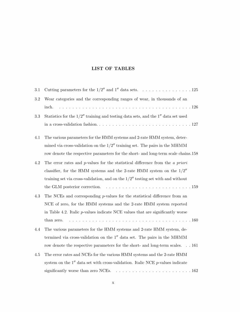
3.1 Cutting parameters for the 1/2′′ and 1′′ data sets. . . . . . . . . . . . . . . . 125
3.2 Wear categories and the corresponding ranges of wear, in thousands of an
inch. . . . . . . . . . . . . . . . . . . . . . . . . . . . . . . . . . . . . . . . . 126
3.3 Statistics for the 1/2′′ training and testing data sets, and the 1′′ data set used
in a cross-validation fashion. . . . . . . . . . . . . . . . . . . . . . . . . . . . . 127
4.1 The various parameters for the HMM systems and 2-rate HMM system, deter-
mined via cross-validation on the 1/2′′ training set. The pairs in the MHMM
row denote the respective parameters for the short- and long-term scale chains.158
4.2 The error rates and p-values for the statistical difference from the a priori
classifier, for the HMM systems and the 2-rate HMM system on the 1/2′′
training set via cross-validation, and on the 1/2′′ testing set with and without
the GLM posterior correction. . . . . . . . . . . . . . . . . . . . . . . . . . . 159
4.3 The NCEs and corresponding p-values for the statistical difference from an
NCE of zero, for the HMM systems and the 2-rate HMM system reported
in Table 4.2. Italic p-values indicate NCE values that are significantly worse
than zero. . . . . . . . . . . . . . . . . . . . . . . . . . . . . . . . . . . . . . 160
4.4 The various parameters for the HMM systems and 2-rate HMM system, de-
termined via cross-validation on the 1′′ data set. The pairs in the MHMM
row denote the respective parameters for the short- and long-term scales. . . 161
4.5 The error rates and NCEs for the various HMM systems and the 2-rate HMM
system on the 1′′ data set with cross-validation. Italic NCE p-values indicate
significantly worse than zero NCEs. . . . . . . . . . . . . . . . . . . . . . . . 162
x
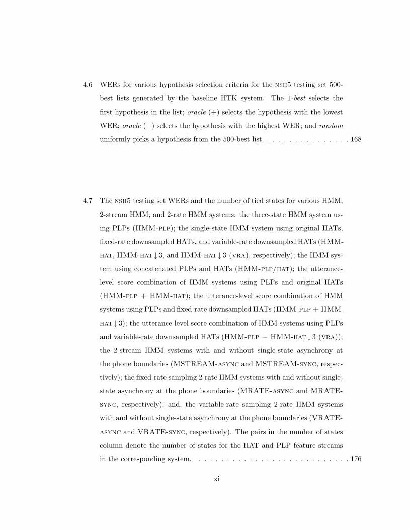
4.6 WERs for various hypothesis selection criteria for the nsh5 testing set 500-
best lists generated by the baseline HTK system. The 1-best selects the
first hypothesis in the list; oracle (+) selects the hypothesis with the lowest
WER; oracle (−) selects the hypothesis with the highest WER; and random
uniformly picks a hypothesis from the 500-best list. . . . . . . . . . . . . . . . 168
4.7 The nsh5 testing set WERs and the number of tied states for various HMM,
2-stream HMM, and 2-rate HMM systems: the three-state HMM system us-
ing PLPs (HMM-plp); the single-state HMM system using original HATs,
fixed-rate downsampled HATs, and variable-rate downsampled HATs (HMM-
hat, HMM-hat ↓ 3, and HMM-hat ↓ 3 (vra), respectively); the HMM sys-
tem using concatenated PLPs and HATs (HMM-plp/hat); the utterance-
level score combination of HMM systems using PLPs and original HATs
(HMM-plp + HMM-hat); the utterance-level score combination of HMM
systems using PLPs and fixed-rate downsampled HATs (HMM-plp + HMM-
hat ↓ 3); the utterance-level score combination of HMM systems using PLPs
and variable-rate downsampled HATs (HMM-plp + HMM-hat↓ 3 (vra));
the 2-stream HMM systems with and without single-state asynchrony at
the phone boundaries (MSTREAM-async and MSTREAM-sync, respec-
tively); the fixed-rate sampling 2-rate HMM systems with and without single-
state asynchrony at the phone boundaries (MRATE-async and MRATE-
sync, respectively); and, the variable-rate sampling 2-rate HMM systems
with and without single-state asynchrony at the phone boundaries (VRATE-
async and VRATE-sync, respectively). The pairs in the number of states
column denote the number of states for the HAT and PLP feature streams
in the corresponding system. . . . . . . . . . . . . . . . . . . . . . . . . . . . 176
xi
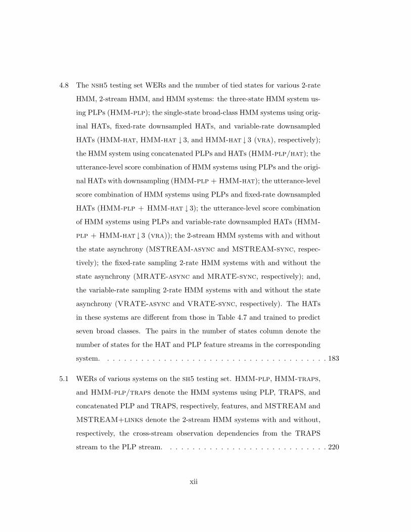
4.8 The nsh5 testing set WERs and the number of tied states for various 2-rate
HMM, 2-stream HMM, and HMM systems: the three-state HMM system us-
ing PLPs (HMM-plp); the single-state broad-class HMM systems using orig-
inal HATs, fixed-rate downsampled HATs, and variable-rate downsampled
HATs (HMM-hat, HMM-hat ↓ 3, and HMM-hat ↓ 3 (vra), respectively);
the HMM system using concatenated PLPs and HATs (HMM-plp/hat); the
utterance-level score combination of HMM systems using PLPs and the origi-
nal HATs with downsampling (HMM-plp + HMM-hat); the utterance-level
score combination of HMM systems using PLPs and fixed-rate downsampled
HATs (HMM-plp + HMM-hat ↓ 3); the utterance-level score combination
of HMM systems using PLPs and variable-rate downsampled HATs (HMM-
plp + HMM-hat ↓ 3 (vra)); the 2-stream HMM systems with and without
the state asynchrony (MSTREAM-async and MSTREAM-sync, respec-
tively); the fixed-rate sampling 2-rate HMM systems with and without the
state asynchrony (MRATE-async and MRATE-sync, respectively); and,
the variable-rate sampling 2-rate HMM systems with and without the state
asynchrony (VRATE-async and VRATE-sync, respectively). The HATs
in these systems are different from those in Table 4.7 and trained to predict
seven broad classes. The pairs in the number of states column denote the
number of states for the HAT and PLP feature streams in the corresponding
system. . . . . . . . . . . . . . . . . . . . . . . . . . . . . . . . . . . . . . . . 183
5.1 WERs of various systems on the sh5 testing set. HMM-plp, HMM-traps,
and HMM-plp/traps denote the HMM systems using PLP, TRAPS, and
concatenated PLP and TRAPS, respectively, features, and MSTREAM and
MSTREAM+links denote the 2-stream HMM systems with and without,
respectively, the cross-stream observation dependencies from the TRAPS
stream to the PLP stream. . . . . . . . . . . . . . . . . . . . . . . . . . . . . 220
xii

ACKNOWLEDGMENTS
I would like to first thank my advisor Mari Ostendorf whom I met at the start of
my graduate studies in Boston University. She has introduced me to statistical pattern
recognition and speech recognition and has provided me guidance and support throughout
my studies. In particular, if I know a few things about experiment design, it is due to her.
She has read this thesis many times, and her comments have significantly improved both the
content and writing of this thesis. I also thank other members of my supervisory committee:
Jeff Bilmes, Maya Gupta, Thomas Richardson, and Don Percival. I have met Jeff Bilmes
early in my graduate studies, and he has been supportive and a source of inspiration since
then. He introduced me to graphical models and information theory. I also thank him for
the careful reading of this thesis and providing GMTK and its support and development,
without which many parts of this thesis would not be realized. I thank Maya Gupta for her
careful reading of this thesis and comments. I thank Thomas Richardson for his comments,
which in particular improved the presentation in Chapter 6, and for agreeing to serve as
the GSR at the last minute. His lectures were always a pleasure to listen to. I thank Don
Percival for his useful comments. His classes that I took early in my studies helped me
shape my research later, and his books were a big influence. I also would like to thank
Julian Besag for always being willing to help.
I thank University of Washington Libraries for their excellent service. I also thank past
and present SSLI and EE computing and administrative staff.
I thank Karim Filali who submitted this thesis to the graduate school and did the
necessary paperwork.
I thank the members of the EARS novel approaches team lead by Nelson Morgan of
ICSI for stimulating discussions, Barry Y. Chen and Qifeng Zhu of ICSI for HAT features
and system design help, and Pratibha Jain and Sunil Sivadas of OGI for TRAPS features.
xiii

The initial experiments with the multi-rate HMMs and their software implementation
developed in this thesis have appeared in [104] for a different milling task, which involved
a collaboration with Randall K. Fish. I thank him for useful discussions about the HMM-
based tool-wear monitoring, and the Boeing Commercial Airplanes, Manufacturing R&D
group, in particular Gary D. Bernard, for sharing their machining expertise and providing
titanium milling data.
This work was supported by the DARPA Grant MDA972-02-1-0024 and Office of Naval
Research Grant ONR-2883401. Needless to say, the views and conclusions expressed in this
thesis are mine and do not necessarily reflect the views of the United States Government or
anyone else for that matter.
xiv

DEDICATION
To my parents and sister.
xv


1
Chapter 1
INTRODUCTION
Humans constantly interact with the environment that they live in. They gather infor-
mation from the natural stimuli that they receive, such as sound and sight. In these sounds
and sights, they recognize spoken utterances and visual objects. Humans perform these
and many other tasks with seemingly no difficulty such that a complete understanding of
how they do it has been elusive. How do humans recognize speech or know that a particu-
lar speaker has spoken? What is it that makes us recognize a familiar face within a large
crowd? Not only do humans solve these problems quite accurately, but they also do it very
fast and simultaneously solve a number of them using a limited resource, the human brain,
whose computational capabilities are well surpassed by today’s computers. However, such
tasks have proven to be very difficult for computers, and the computer’s performance lags
much behind that of humans. The gap especially widens as the tasks to which we apply
our algorithms become more unconstrained and realistic. For example, the state-of-the-art
speech recognition algorithms can achieve error rates less than 1% when tested on digit
sequences recorded in laboratory conditions, but the same algorithms give error rates about
20 − 30% for casual conversation speech recorded over a telephone [181]. Similar perfor-
mance degradations are observed in the presence of noise and other adverse conditions. In
contrast, humans are robust and adaptive across a variety of tasks and conditions, and their
performance gracefully degrades.
As computers get more and more powerful, the idea that computers can hear, see,
talk, understand, etc., in short, have a human-like interface, and perform these tasks on a
scale and capacity that humans cannot, is no longer a science-fiction notion but a practical
necessity. Such an interface provides a natural way to access to the wealth of information

2
stored in information networks such as the internet, and services such as machine translation
and telephone banking. In addition, once the technology is available, a computer can
perform such tasks on a scale and capacity that humans cannot, such as scanning hundreds
of hours of news audio to find segments about a particular topic, or retrieving images with
a particular content from a large database.
The idea that computers can imitate and rival humans has been a provocative topic
since the invention of computers, and it sets an ultimate challenge to our basic understand-
ing of human intelligence, learning, understanding, decision making, hearing, vision, and
so many other tasks that humans can or learn to do. The type of problems that this the-
sis is concerned with is of the latter kind, namely hearing and vision, which are relatively
well-defined and essentially pattern classification or recognition problems, where the goal
is to classify an object into one of pre-determined categories. Pattern classification prob-
lems range from general perception tasks that we mentioned above to specific industrial
or commercial problems, such as recognizing word sequences underlying spoken utterances,
recognizing speakers from their voices, segmenting natural and man-made regions of aerial
images, recognizing characters in handwritten documents, detecting the amount of wear on
cutting tools from machining vibrations, detecting fraud on credit-card interactions, etc..
Pattern classification problems appear everywhere, each with a special structure and pecu-
liarity. Then, the question we are interested in is: how can we program a computer to solve
a particular pattern classification problem, such as automatic speech recognition?
The prevalent framework for solving pattern classification and other problems involving
decision making under uncertainty and incomplete information is probability theory and
statistics. Probabilistic approaches are especially useful in highly complex yet structured
domains with many degrees of freedom, such as speech and natural language and images.
For any particular classification problem, it may not be obvious where uncertainty and
randomness lies. In many cases, they are inherent to the world, and in others, they arise as
a representation of our limited knowledge about the world. For example, each speaker has
a unique glottis and vocal tract shape, which produce sounds when air is flown from the
lungs. There are also sources of uncertainty such as the air turbulence from the lungs and
the precise configuration of the vocal tract apparatus, and these cause random variations

3
in the produced acoustic signals. No two realizations of a spoken utterance are the same,
even if they are consecutively produced by the same speaker, and it is next to impossible
to form a deterministic relationship between the parameters of speech production such as
the speaker and linguistic message, and the produced acoustic signals. Instead, in the
statistical approach, these parameters and the produced acoustic signal are represented as
random variables and their relationships to each other are probabilistically formulated. The
result is a stochastic model of speech production, which can be used to infer speakers from
their voices or decode linguistic messages underlying spoken utterances.
1.1 Statistical Models for Pattern Recognition
Models characterize the statistical regularities of features coming from objects in each clas-
sification category, and during classification, they are used to determine the class which is
most plausible based on the observed evidence, features. As such, the models we use for
pattern classification should be appropriate for this purpose. In practice, we rarely know
which model to use, and the models are usually chosen based on a combination of prior
knowledge and data. First, prior knowledge, in consideration with computational complex-
ity and mathematical tractability, may suggest one or more model families. Second, a data
set consisting of examples of pairs of features and class labels is used to estimate the free
parameters of the hypothesized model and/or select among alternative model hypotheses.
Model selection is usually an iterative process, where hypotheses are modified based on the
performance of previously hypothesized models. These two levels of inference, first designing
a model and second estimating its parameters, form the basis of building statistical models
for pattern classification or any other field involving data modeling. There are a number
of practical and theoretical challenges in inferring accurate models for pattern classification
applications and this thesis concerns with these challenges.
One of the central problems in data modeling is how to model complex, large-scale sys-
tems such as speech and natural language. Even though there usually exists some knowledge
about specific components of the system or specific cases, such knowledge in most cases is
difficult to place in a probabilistic setting or not sufficient to specify a complete probabilistic
4
model. In addition, it usually brings more harm than benefit to incorporate an incorrect
piece of knowledge into the modeling process, rather than not to use any knowledge at
all. This is one of the main causes for the paradigm shift from knowledge- or rule-based
methods to statistical, data-driven methods in complex applications such as speech recog-
nition, computational linguistics, and handwritten character recognition. In the statistical
approach, the models are learned from data by finding the statistical regularities observed
in instances from objects coming from different classes. However, training data is usually
limited as compared to the complexity of the phenomena to be modeled, and it becomes
crucial for models to extract the structures and relationships that are generalizing instead
of those specific to the training data and noise. Overly complex models can quickly overfit,
whereas simple models might not have sufficient complexity to learn any interesting struc-
ture. Thus, it is necessary to use parsimonious models that can extract structure from data
in an efficient manner, as opposed to arbitrarily increasing complexity of simpler models.
Modularity (where systems are built out of simpler components) and hierarchy (where sys-
tems are decomposed into scale-based parts) are the two main design principles to treat
complicated systems in simple ways for both statistical and computational reasons. Modu-
larity and hierarchy are also characteristics of many interesting signals such as speech and
images. For example, a small number of sound units called phones almost universally form
the basic building blocks of human speech, and language is hierarchically organized from
phones to words to sentences to larger units of language.
Determining structural details of the model (such as model order and dependencies) is
also a central problem in pattern classification applications, generally referred to as model
selection. In a typical application, a combination of prior knowledge about the domain,
computational and mathematical tractability, and statistical efficiency suggests that a model
be chosen among a set of alternative model hypotheses. Typically, we want to find the
model in a large class of models that will perform the best in our pattern classification
problem. Alternative hypotheses in model selection may involve, among other parameters,
any structural assumptions made about the stochastic model relating classification features
to class labels, such as interrelationships between features and the class indicator, their
statistical characteristics, and hidden or causal data generation mechanisms. Given a set of

5
such alternative hypotheses, which one should we select for a specific pattern classification
at hand? The model selection is usually performed by optimizing an objective function
over a training data set, such as how well the model describes the training data. The
ultimate goal in pattern classification is the prediction of class labels from features, and thus,
models should be chosen based on how well they predict and discriminate between objects
from different classes. Unlike purely data modeling approaches which treat all variables,
features and class indicator in pattern classification, on an equal footing, a different approach
emphasizing prediction of classes from features is necessary for pattern classification. The
objective function used in model selection should be indicative of the performance of the
model for predicting classes.
Another challenge in pattern classification is the estimation of parameters of the model
from data once a particular model structure has been chosen. The argument that models
should be chosen based on how well they predict classes from features, applies equally well
to parameter estimation. Parameter estimation is usually done by optimizing an objective
function such as the likelihood of data with respect to parameters. The objective func-
tion used for parameter estimation should adjust model parameters such that the resulting
model is effective in discriminating between classes. Unlike likelihood-based criteria such as
maximum likelihood which decouple parameter estimation across different classes, discrim-
inative criteria necessarily consider all classes simultaneously, and parameters associated
with different classes are coupled together during parameter estimation. As a result, dis-
criminative parameter estimation methods are in general computationally more expensive
than likelihood-based methods. Moreover, discriminative objective functions such as the
empirical error rate and the conditional likelihood of class labels given features are difficult
to optimize, and they do not enjoy many of the properties that are desirable in optimiza-
tion, such as monotonic convergence and lack of any learning rates or other tweak factors.
This is in contrast with the likelihood-based parameter estimation methods such as the
expectation-maximization algorithm.
The overall objective of this thesis is to build statistical models for pattern classifi-
cation problems. In particular, we are interested in statistical model inference, and our
contributions lie in the modeling challenges that we have stated above and in three complex
6
applications, automatic speech recognition, speaker verification, and machine tool-wear con-
dition monitoring. First, we develop a parsimonious multi-scale modeling architecture for
stochastic processes that exhibit scale-dependent characteristics and long-term temporal de-
pendence. In this multi-scale extension of popular hidden Markov models, multi-rate hidden
Markov models, multi-scale processes are characterized using scale-based state and obser-
vation sequences. Second, we develop a model selection algorithm for statistical modeling
in pattern classification applications. In this algorithm, the dependency structures in the
models that relate each classification feature to other features and class indicator are chosen
so as to maximize separability between objects from different classes. Third, we develop
a new mathematical approach to a common discriminative parameter estimation method
based on the conditional likelihood function, which provides theoretical justification for the
practical implementations of this method and suggests modifications for faster convergence.
Moreover, we present a few new results about the expectation-maximization algorithm, a
commonly used maximum likelihood parameter estimation method with hidden data, most
notably its equivalence to a first-order gradient-descent algorithm in the exponential family
and faster-converging variants suggested by a new derivation. We review these and other
theoretical and experimental contributions of this thesis below.
1.2 Contributions
1.2.1 Multi-rate Hidden Markov Models
Processes that evolve at multiple scales are common, e.g. human language, speech, natural
scenes, and machining vibrations. Human language also has a hierarchical structure ranging
from a small number of phones being the basic building blocks of words to phrases and to
larger units of language. Speech is characterized by effects from multiple time scales, such
as utterance-level effects due to speaking rate, syllable-level effects due to lexical stress, and
millisecond-level effects due to phonetic context. In metal cutting operations, e.g. milling,
the short-time behavior of machining vibrations is determined by long-term effects such
as the amount of wear on the cutting tool and “noisy/quiet” cutting periods in titanium
milling [81].
7
In signal processing, it has been long recognized that a scale-based analysis at various
resolutions of time is efficient for compression or coding of signals and images as well as signal
recovery from noise [259]. Wavelets, subband coding, and perceptual audio coding are a
few such methods. In statistics and machine learning, hierarchical structures are also found
to be key to be able to reveal and learn long-term dependencies in temporal processes and
parsimoniously represent complex and large systems such as spoken language. Given a finite
amount of training data, models which account for variability and dependency associated
with the progress of a system at various scales might be more effective for extracting multi-
scale structure from data, since they judiciously distribute the model complexity instead
of a brute force approach of increasing the complexity of simple models. Such a multi-
scale approach typically forms the basis of modeling complex, real-world processes such
as spoken language which current speech recognition systems represent by characterizing
allowable state sequences via a hierarchy of models from sentences to words to phones.
A popular approach to modeling sequence data with temporally changing characteristics
is state-space modeling such as hidden Markov modeling and linear dynamical systems. In
state-space models, a sequence of hidden states represents the temporally changing charac-
teristics of the process, and observations (i.e. time-series) are assumed to have statistical
regularities conditional on these hidden states. Hidden states typically follow a Markovian
dynamics and propagate the context information. Such a doubly-stochastic representation
of time-series via an underlying hidden state sequence is a powerful modeling tool, and hid-
den Markov models (HMMs) and other state-space models are popularly used for modeling
a variety of signals, including speech [225], weather patterns [149], biological sequences [93],
and images [179]. However, as powerful as they are for modeling temporal data, HMMs are
limited in their power for modeling multi-scale processes due to the use of single-component
state and observation spaces in representation, where scale-based components of a multi-
scale process need to be factored together. Representation of multi-component state spaces
in a multi-scale stochastic process by an HMM requires assigning a unique state to each
possible state combination, which results in a surfeit number of parameters and excessive
computational cost. Similarly, representation of multi-scale observation sequences in an
HMM requires their synchronization by oversampling coarser scales. Oversampling adds
8
redundancy and oversampled observation sequences when used in an HMM might severely
violate HMM’s modeling assumption that observations in an HMM are conditionally inde-
pendent of each other conditional on hidden states. Violating HMM’s modeling assumptions
may or may not have an impact on classification performance in terms of classification accu-
racy, but introduction of redundancy by oversampling results in overconfident classification
decisions due to counting the evidence from coarse scales multiple times, so oversampling
is harmful for many applications where the a posteriori probability or confidence of the
decision is also required.
Our contribution to multi-scale stochastic modeling is the development of multi-rate
HMMs which are a multi-scale extension of HMMs for characterizing temporal processes
evolving at multiple time scales. Similar to an HMM, a multi-rate HMM is a state-space
model and characterizes the non-stationary process dynamics via a hidden system state.
However, unlike an HMM, a multi-rate HMM factorially represents the system state at
multiple time scales and decomposes observational variability into corresponding scale-based
components. State and observation spaces are hierarchically organized in a coarse-to-fine
manner, efficiently representing short- and long-term context information simultaneously
and facilitating intra- and inter-scale couplings across time and scale. Yet, due to the hi-
erarchical model structure, training and decoding of multi-rate HMMs are computationally
efficient. In pattern classification problems, the multi-rate HMMs provide better class a
posteriori probability estimates and confident classification decisions than an HMM operat-
ing at the finest time scale involved (due to not overcounting evidence from slowly varying
scales by oversampling).
We will apply multi-rate HMMs to wear modeling in machine tool-wear condition mon-
itoring and acoustic modeling in automatic speech recognition. Both processes and speech
acoustics exhibit multi-scale behavior. In machine-tool wear monitoring, multi-rate HMMs
will be used for characterizing long-term “noisy/quiet” transient behavior as well as the
short-term vibrations due to material removal and chatter observed in titanium milling. In
acoustic modeling, they will be used for integrating long-term temporal information from
syllable time scales with short-term spectral information from phones, as currently employed
by HMM-based speech recognizers. In particular, we will use a 2-rate modeling architec-
9
ture to represent syllable structure and lexical stress in combination with phones for better
characterizing acoustic variability associated with conversational speech. For both recogni-
tion tasks, we will show that multi-rate HMMs improve over HMMs or other models that
are not scale-based, in terms of both classification accuracy and confidence of classification
decisions.
1.2.2 Model Selection for Statistical Classifiers
In the absence of any prior knowledge in favor of one model over the others, model selection
refers to a data-based choice among competing models. The fundamental problem in model
selection is to balance model complexity against the fit to the data. Models with oversim-
plistic assumptions might be too restrictive to extract interesting structure from data, while
arbitrarily complex models might easily overfit to a particular data set and not generalize
well. Model selection is central to any statistical problem involving data, and there is a
large body of literature about model selection in statistics. Much of the previous work in
model selection is concerned with finding models that best describe a given data set, and
as such, they are mostly based on likelihood criteria. In likelihood-based methods such as
minimum description length and likelihood-ratio testing, models are chosen with respect to
the probability that they assign to the training data set, in combination with a mechanism
to penalize complex models. The likelihood-based approaches are optimal in the sense that
they would recover the true probability distribution that generated data, if this distribution
is among the model hypotheses, and if the amount of training data is unlimited. However,
neither assumption holds in practice. In addition, considerations such as computational
complexity and mathematical tractability are also factors in determining model hypotheses.
As a result, a goal-oriented approach in which models are selected based on the ultimate
job they are used for in a given application, could be more robust to incorrect modeling
assumptions. In pattern classification, one of the ultimate goals is the prediction of class
labels from features, and as such, models should ideally be chosen based on how well they
predict.
Our contribution to model selection for pattern classification problems is a formulation

10
of a discriminative model selection criterion and its employment for classifier design within
the graphical modeling framework where graphs encode probabilistic dependence relations
among the variables of the model and determine a factorization of their joint distribution
into local factors of variables. Given that the goal in pattern classification is accurate
classification, one ideally wants to use the classification error rate as the objective function
to score alternative models. However, the error rate is a non-smooth function and does
not easily lend itself to optimization. For example, the error rate of a classifier specified
as a graphical model does not factorize with respect to graph structure, preventing the
use of local search algorithms in the dependency structure search for the graphical model.
Instead, we propose the conditional likelihood of class labels given features as the model
selection criterion. As compared to joint likelihood of class labels and features which does
not discriminate between class labels and features (as used in the likelihood-based model
selection methods), conditional likelihood function emphasizes the prediction of class labels
from features, and hence, it is discriminative. Moreover, the maximum conditional likelihood
criterion is consistent with the goal of predicting confidence of classification decision, as it
directly optimizes the class a posteriori probabilities.
The particular model selection problem in pattern classification that we are interested in
is dependency modeling, and graphical modeling provides a convenient framework for explor-
ing discriminative dependency structures for pattern classification. In graphical modeling
for pattern recognition, we use graphs to specify statistical models relating classification
features to labels, and the graphical models allow us to express a variety of modeling prob-
lems in classification, such as feature selection, auxiliary feature modeling, and dependency
modeling, via a common object, the graph structure. We apply the maximum condition
likelihood criterion to the graph structure selection for a graphical model to find sparse
dependency structures that give better class discrimination. For model selection, graphical
models naturally deal with the fundamental issue of model complexity, as determined by
graph sparsity. Sparser graphs result in simpler factorizations of a multivariate distribution
and hence smaller number of parameters and lower computational cost of probabilistic in-
ference. The conditional likelihood score of a graphical model partially decomposes with
respect to the graph structure, and this decomposition allows for the employment of local
11
or approximate search methods. Within the context of the naive Bayes classifier (a particu-
larly simple yet competitive classifier with strong independence assumptions [197]), we will
illustrate that the maximum conditional likelihood structure selection criterion for graph-
ical model classifiers provide intuitive and practical solutions to a variety of dependency
modeling problems in classification, including feature selection, auxiliary feature modeling,
and dependency modeling.
The utility of the conditional maximum likelihood dependency selection algorithm that
we develop lies in inferring low-complexity discriminative models for pattern classification
problems. We use it for enhancing the multi-stream coupled HMMs popularly used in
acoustic modeling for speech recognition. In the multi-stream models, the features coming
from different signal processing techniques or information sources such as audio and vision
are used in parallel for predicting spoken words underlying an utterance. However, the basic
multi-stream model assumes that feature streams are independent of each other conditional
on the underlying hidden states, which is unrealistic for some feature combinations, and
we will use the dependency selection algorithm to sparsely augment the basic multi-stream
model with direct cross-stream dependencies between feature streams, whenever they are
most helpful for recognition.
1.2.3 Parameter Estimation for the Exponential Family
The argument in the previous section that models should be selected to maximize the class
discrimination in pattern classification applies equally well to parameter estimation. By
parameter estimation, we mean estimation of free parameters of a model once a particular
model family is chosen, such as the mean vector and covariance matrix in a multivariate
Gaussian distribution. The popular maximum likelihood estimation is statistically con-
sistent under the model correctness and infinite training data assumptions; it decouples
the parameter estimation across classes; and it usually results in many mathematically
tractable class-based small optimization problems. However, these assumptions rarely hold
in practice, in which case maximum likelihood parameter estimation is no longer optimal for
pattern classification problems. Indeed, discriminative parameter estimation methods based
12
on minimum classification error rate and maximum conditional likelihood are regularly used
in current speech recognition systems and consistently improve recognition accuracy over
maximum likelihood methods [267]. In this thesis, we will focus on the maximum condi-
tional likelihood as our discriminative parameter estimation criterion for the same reasons
that we use it for discriminative model selection: it is smooth and relatively tractable as a
function of parameters.
Unlike the likelihood function, the conditional likelihood function couples parameters
associated with different classes, and during parameter estimation one needs to consider all
classes simultaneously. In addition, all of training data (not just the portion with examples
coming from a particular class) are used in estimating parameters of each class. As a result,
conditional likelihood maximization is computationally more expensive. In addition, many
estimation methods, such as the extended Baum-Welch training of HMMs (see, e.g. [244]),
require that the learning rate in iterative maximization of the conditional likelihood function
be infinitely small to achieve monotonic convergence of the conditional likelihood function.
However, in practice, it has been observed that convergence can be achieved for relatively
large learning rates, and as such, there is a gap between theory and practice of maximum
conditional likelihood estimation.
Our contribution to discriminative parameter estimation is the development of a new
mathematical approach to maximum conditional likelihood estimation in the linear expo-
nential family (which is an important class of parametric distributions including HMMs and
Gaussian mixture models that are extensively used in practice) based on a recent optimiza-
tion method, the concave-convex procedure [278]. The crux of our approach to maximum
conditional likelihood parameter estimation is a decomposition of the conditional likelihood
function into convex and concave parts and the application of the concave-convex optimiza-
tion procedure on these parts. The resulting iterative concave-convex procedure involves
solving a convex optimization problem at each iteration, which cannot be done analytically,
but the fixed points of these problems are similar in form to the updates of popular ex-
tended Baum-Welch training. Most importantly, our approach gives insight into how to
choose the learning rate in the update equations for fast, monotonic convergence and shows
that reasonable rates of convergence can be obtained without setting the learning rate to

13
very small values. As such, our approach to maximum conditional likelihood estimation
provides a theoretical justification for the current practice of maximum conditional likeli-
hood parameter estimation in the speech recognition literature and closes the gap between
the theory and practice of maximum conditional likelihood estimation.
To verify our claims about the convergence behavior of conditional maximum likeli-
hood parameter estimation and its effectiveness for pattern classification, we will apply
this estimation procedure to a speaker verification task. In this task, they will be used for
discriminatively estimating the parameters of the large-dimensional mixture of Gaussian
speaker models.
We will also make a number of contributions to the theory and practice of expectation-
maximization (EM) algorithms [87, 191] in the linear exponential family using the same tools
that we use for developing the maximum conditional likelihood parameter estimation. The
EM algorithm is an iterative method for maximum likelihood parameter estimation with
incomplete data, such as unobserved mixture variables in mixture models or states in state-
space models. The EM algorithm is extensively used in a variety of applications ranging from
speech recognition to image processing. The popularity of the EM algorithm mainly stems
from the fact that it provides closed-form parameter updates when applied in the linear
exponential family and that the updates are guaranteed to converge to a local maximum
of the likelihood function. The convergence of the EM algorithm is essentially determined
by the ratio of the amount of missing information to the amount of complete information,
and it can be slow if the amount of missing information is high. As a result, there is a
large body of work in the literature on how to accelerate the EM algorithm. In addition,
the updates of the EM algorithm reveal no direct relationship to the more general gradient-
descent numerical optimization algorithms. However, our approach to maximum likelihood
parameter estimation in the exponential family, based on the concave-convex optimization,
reveals an interesting connection between the EM algorithm and gradient-descent methods
and also allows us to formulate faster-converging variants of the EM algorithm and shed
new light on its susceptibility to local maxima.
First, we provide a new derivation of the EM algorithm in the linear exponential family
using the previously mentioned concave-convex optimization procedure. The new derivation
14
suggests a family of EM-type algorithms with varying rates of convergence, in which the
usual EM algorithm is a point. In this family of algorithms, there are slowly converging
versions as well as faster versions than the EM algorithm. The different members of the
family arise from alternative concave-convex decompositions of the likelihood function, and
some decompositions result in faster converging algorithms, especially when the amount of
missing information is high.
Our concave-convex optimization formulation of the maximum likelihood parameter es-
timation in the exponential family also reveals that all EM algorithms in this family are
in fact a particular kind of first-order gradient-descent algorithm. This result generalizes
similar results in the literature for specific distributions such as the mixture of Gaussian
distributions [270]. Using this equivalence result, we also provide a result about the suscep-
tibility of EM algorithms to poor initializations and local maxima.
1.3 Outline of the Thesis
This thesis is organized in seven chapters. Chapter 2 develops the theoretical foundations
for our work, and Chapter 3 describes our applications and the experimental paradigms
used in our tests. The three subsequent chapters describe the core of this thesis: our
contributions to multi-scale statistical modeling, model selection for pattern classification,
parameter estimation for the exponential family, and the applications of the developed
methods and tools to acoustic modeling for speech recognition, speaker verification, and
machine tool-wear monitoring. These three chapters can be largely read independently of
each other. Chapter 7 is the conclusions and summary chapter.
In Chapter 2, we will set the theoretical background for our work and introduce con-
cepts and terminology used in the later chapters. We will describe the statistical pattern
classification framework and give an overview of various issues involved in designing pattern
classification systems. We will discuss commonly used parameter estimation methods from
a pattern classification point of view and describe the expectation-maximization algorithm,
as it sets the background for our work about discriminative parameter estimation. Next we
will introduce statistical modeling tools that we will use in our work, namely exponential

15
family distributions, hidden Markov models, and graphical models. The exponential family
is an important class of parametric distributions whose analytical properties will be heavily
exploited in our work about parameter estimation. The hidden Markov model is a popularly
used model for nonstationary time-series and our starting point for our multi-rate extension
in Chapter 4. Graphical modeling is a formalism for model specification via graphs, and
most models in this thesis will be analyzed from that point of view. In addition, the graphi-
cal modeling framework is central to the model selection work in Chapter 5. Chapter 2 will
continue with a discussion of model selection methods, first from a general data modeling
perspective and next from a pattern classification perspective. We will describe various
model selection criteria proposed in the literature and pay particular attention to model
selection for graphical models. Chapter 2 finishes with a brief introduction to information
theory.
In Chapter 3, we will describe our applications, namely automatic speech recognition,
speaker verification, and machine tool-wear condition monitoring. For each application, we
will explain the particular pattern classification problem involved and give an overview of
various modules that go into the design of a complete system architecture. The descrip-
tions of system architectures will include details of feature extraction methods from sensory
signals, commonly used statistical models, and the decision making process during classi-
fication as well as the evaluation metrics. In this chapter, we also give the experimental
paradigms adopted for the experiments in the later chapters. For each application, we will
describe the specifics of tasks associated with the experimental work reported here, includ-
ing data and training and testing procedures. We will also provide the implementation
details for the baseline system architectures.
In the first part of Chapter 4, we will introduce the multi-rate hidden Markov models
as a multi-scale extension of hidden Markov models for the parsimonious characterization
of processes evolving at multiple time scales. We will give solutions to their probabilistic
inference and parameter estimation problems and compare them to previously proposed
multi-scale and other related models. We will also introduce a number of extensions to the
basic multi-rate HMM framework for allowing variable-rate sampling schemes and richer
set of cross-scale interactions. In the second part of Chapter 4, we will apply multi-rate
16
hidden Markov models to first, statistical modeling of wear processes for machine tool-wear
monitoring and second, acoustic modeling for speech recognition, and present experimental
results. In wear process modeling, they are used for characterizing long-term “noisy/quiet”
transient behavior associated with titanium milling, whereas in acoustic modeling, they are
used for joint modeling of speech at phone and syllable time scales in a number of alternative
modeling schemes.
In Chapter 5, we will introduce a discriminative model selection criterion for statistical
classifiers, where models are evaluated with respect to the conditional likelihood of class
labels given features in a training data set. In an application of the proposed model selection
criterion, we will consider classifiers as specified by graphical models and optimize the graph
dependency structures of the graphical models so that features become most predictive of
the class labels. We will analyze instantiations of this method in the context of the naive
Bayes classifier and in its various extensions for feature selection, auxiliary feature modeling,
and dependence modeling. We will present an application of the proposed model selection
algorithm for better utilizing multiple feature streams by direct cross-stream dependencies
in multi-stream acoustic modeling for speech recognition and report experimental results.
In Chapter 6, we will present our work about statistical parameter estimation for the
exponential family. In the first part of this chapter, we will use an optimization tool, concave-
convex optimization [278], for deriving a discriminative parameter estimation algorithm
based on maximizing the conditional likelihood function for the exponential family. The
resulting iterative algorithm is similar to the algorithms that have appeared in the literature
for the same problem, but the new derivation is important in giving theoretical justification
for the current implementations of this method as well as providing insight to choosing
learning rates for fast, monotonic convergence. We will demonstrate the effectiveness of the
proposed algorithm and learning rate schedules in a speaker verification task, where they
will be used for estimating the parameters of mixture of Gaussian speaker models. In the
second part of Chapter 6, we will present a new derivation of the expectation-maximization
algorithm using the same analytic tool, the concave-convex optimization. The new analysis
of the expectation-maximization algorithm will shed more light into convergence properties
and suggest faster-converging variants. In addition, it will allow us to prove a few new results

17
about the expectation-maximization algorithm in the linear exponential family, including
its equivalence to a first-order gradient descent algorithm and its susceptibility to local
maxima.
Finally, we will conclude in Chapter 7 by giving a summary of our work as well as
discussing its limitations and future research directions suggested by it.
18
Chapter 2
THEORETICAL FOUNDATIONS
In this chapter we give the theoretical background for our work in the later chapters
and introduce various tools and concepts that will be frequently encountered. The various
developments introduced in this thesis revolve around a central concept: statistical model
inference for pattern classification, a term that we use to indicate for both selecting a model
and estimating the parameters of the selected model. Overall, we are mainly interested in
classification problems involving highly structured temporal data such as speech, inference
of their accurate models from data, and their parameter estimation.
This chapter is organized as follows. We will first review the statistical pattern recog-
nition framework and introduce the model selection and parameter estimation problems in
model inference from data. We will then describe various optimization criteria commonly
used for parameter estimation and discuss the extent to which they are appealing from a
pattern classification perspective. We will then introduce the expectation-maximization al-
gorithm, widely used for maximum likelihood parameter estimation in the presence of miss-
ing data, and used here in our experiments and algorithm analysis. Next, we will provide a
brief introduction to exponential family distributions and describe their various properties,
which will be useful for some of our theoretical work. We will describe a particular model
for temporal data, the hidden Markov model (HMM), in detail, as it is the starting point
for its multi-scale extensions introduced in Chapter 4 and central to our applications. Next,
we will introduce the graphical modeling framework that will be used for model comparison
and specification throughout this thesis. We will then discuss model selection, first from a
general data modeling perspective and second from a pattern classification perspective, and
in particular for graphical models. Lastly, we will give a brief primer on information theory
to define various information-theoretic concepts that will be regularly used.

19
2.1 Notation
In this section we will describe the commonly used notation. We denote random variables by
uppercase letters such as X and Y and the specific values that they take by lowercase letters
such as x and y. We will use the blackboard bold letters to denote the state spaces of random
variables such X ∈ X. We will typically use p and q to denote probability distributions such
as p(X) for X with the probability law p. To simplify the notation, we will avoid explicitly
referring to the random variables in probability distributions, for example we use p(X) and
p(Y ) as shorthands for pX(X) and pY (Y ), respectively. We will use Ep [f(X)] to denote
the expectation of the function f(X) with respect to the distribution p(X), and drop the
subscript p in cases where p is obvious from the context. We will use var [g(X)] to denote
the variance of g(X), cov [h(X)] to denote the covariance matrix of vector-valued h(X),
and cov [h(X)|Y = y] to denote the covariance matrix of h(X) given Y = y.
We will typically use calligraphic letters to denote the collections of independent, and
identically distributed (i.i.d.) samples such as X ≡ {X1, . . . , XN}, or shortly X ≡ {Xn}Nn=1,
for a sample size N . In general, we will denote a set with elements θa indexed by a parameter
a in an another set A, by {θa}a∈A and use the subscript t to index temporal sequences and
n to index i.i.d. samples. In cases where the index set is obvious, we will drop it, as in
using {Xn} as short for {Xn}Nn=1. We denote the vector space of d-dimensional real vectors
by Rd.
The notation 1{·} refers to the indicator function, and 1{s} is equal to one if the
statement s, e.g. x = y, is true, and it is equal to zero otherwise. The notation δi,j refers to
the Kronecker delta function, and it is equal to 1 if i = j and zero otherwise. The cardinality
of a set A will be indicated by |A|.
2.2 Statistical Pattern Classification
Pattern classification or recognition is about the determination of an unknown discrete
nature of an object, called class, from its features. Recognizing the word sequence underlying
a spoken utterance, recognizing speakers from their voices, segmenting natural and man
made regions of aerial images, and predicting of the wear status of a milling tool from
20
its machining vibrations are all examples of pattern classification tasks. Our scientific
knowledge about the physical processes underlying these phenomena is almost always not
sufficient to specify deterministic mappings from features of objects to their class labels. In
addition, the association between class labels and features can be inherently random and/or
uncertain. In the statistical approach, such limited knowledge and/or inherent randomness
are represented by a probability distribution over classification features and class labels,
and optimal classification decisions are made to minimize the expected risk of classification
decisions with respect to the underlying distribution.
More formally, we denote the class label by C ∈ C, and the classification features by
X ∈ X, and their joint probability distribution by p(C,X). We also define a loss function
L(c, c′) specifying a penalty for classifying an object as class c′ when in fact it belongs to
class c. The decision rule or the classifier is a mapping from the features X to the classes
C: α(X) : X→ C. The expected cost of a decision rule α(X) at an object with the features
X = x is given by
R(x) ≡ E [L(C,α(x))|X = x] (2.1)
where the expectation is with respect to p. Given an explicit form for the loss function
L(c, c′), the optimal classification rule α∗(X) minimizing expected loss in Equation 2.1 can
easily be found [92, 45, 88].
A popular loss function is the 0/1 error function, L0/1, which does not incur any penalty
for correct classification decisions and penalizes all incorrect classification decisions equally:
L0/1(c, c′) ≡
1 if c 6= c′,
0 otherwise.
For the 0/1 loss function, the expected loss becomes equal to the probability of error,
R0/1(x) ≡ p(C 6= α(x)),
and the optimal decision rule achieving minimum probability of error is given by
α∗0/1(x) ≡ argmaxc∈C
{p(C = c|X = x)} , (2.2)

21
or equivalently by
α∗0/1(x) = argmaxc∈C
{p(C = c,X = x)} , (2.3)
since the marginal probability of features p(X = x) does not depend on C. Hence, the
decision rule with the minimum probability of error is intuitively given by selecting the class
having the highest a posteriori probability given the features. The rule α∗0/1 in Equation 2.2
is commonly referred to as Bayes optimal decision rule [92, 45, 88].
Decision theory provides optimal procedures for classification once we know the prob-
abilistic characterization of classes and features. However, in practice, such exact charac-
terizations are often not available or only partially so, and they need to be inferred from
data. Even though the conditional distribution p(C|X) is sufficient for classification (see
Equation 2.2) whether one infers the full joint distribution p(C,X) or only the conditional
distribution p(C|X) from data gives rise to generative and conditional modeling, respec-
tively, paradigms in pattern recognition [156]. Conditional modeling is more direct and
focuses on the mapping from features X to class C, ignoring marginal distribution of fea-
tures p(X), which is irrelevant for classification. On the other hand, generative modeling is
more intuitive and allows for the incorporation of prior knowledge into the classifier design.
It results in modular models that can parsimoniously characterize very large, complex do-
mains such as human speech and language. In addition, generative models are more flexible
than their conditional counterparts and can easily handle, for example, missing data and
variable-size feature sequences, e.g. spoken utterances of arbitrary duration. The parame-
terization of generative models is usually simpler, and their estimation from data tends to
be easier. Moreover, the knowledge of the joint distribution is also useful for purposes other
than classification such as completing missing data. Due to these reasons, we will work in
the generative modeling framework in designing pattern classification systems and try to
infer generative models with good class discrimination capabilities.
In the generative approach, the modeling of joint distribution p(C,X) is done by factor-
ing it into the a priori class probability distribution p(C) and the class-conditional feature
distribution p(X|C) components:
p(C,X) = p(C)p(X|C).
22
Modeling of the a priori class probabilities p(C = c) is relatively easy, and they can be
obtained, for example, from the relative frequencies of each class in the training data set.
However, modeling of class conditional distributions is more challenging due to the fact
that features X are usually large dimensional and the amount of training data available
for estimation is limited. The problem can be alleviated by restricting the conditional
distribution p(X|C) to be in a family of distributions F and finding the best possible fit
within this family according to some criteria. In parametric density modeling, the distri-
butions are restricted to a certain parametric form and the model family Fθ is indexed
by a parameter vector θ [88]. For example, the family Fθ can be multivariate Gaussian
distributions with a particular covariance structure. In parametric modeling, the density
estimation problem reduces to that of much simpler parameter estimation, but the para-
metric form assumed by the family Fθ amounts to making certain structural assumptions
about the class-conditional distributions. In this thesis, we will use parametric models for
class-conditional distributions, which will involve both selection of an appropriate model
family, called model selection, and estimation of the parameters within the selected family,
called parameter estimation. For good classification performance, it is important that both
the model and its parameters be selected according to a criterion that is directly coupled
with the classification accuracy, an issue that we will discuss in detail in the coming sec-
tions and propose solutions for in the latter chapters. In the next section, we will review
statistical criteria commonly used for parameter estimation in pattern classification tasks
and later discuss model selection in Section 2.8 after we introduced the modeling tools such
as graphical modeling that we will use for statistical modeling in this thesis.
In passing, we note that there exist non-probabilistic approaches to pattern classification
as well, which directly model the mapping from classification features to class labels by a
general discriminant function without any appeal to probability distributions, e.g. k-nearest
neighbors classifiers [92], neural networks [45], support vector and kernel machines [57],
etc.. There also exist hybrid schemes that use generative models within discriminative
classifiers, e.g. the Fisher scoring method for feature extraction for kernel machines [151],
and maximum entropy discrimination [152], and vice versa, e.g. the neural network and
HMM hybrids in speech recognition [49].
23
2.3 Parameter Estimation
Suppose that we have chosen a parametric family Fθ for class-conditional probability distri-
butions pθc(X|C = c), c ∈ C and have a training data set ofN examples, D ≡ {(Cn, Xn)}Nn=1.
How should the parameters θ ≡ {θc}c∈C be estimated for achieving high classification accu-
racy when the resulting distributions are used as plug-in estimates in the Bayes decision rule
in Equation 2.2? In this section, we will present three parameter estimation principles: max-
imum likelihood, maximum conditional likelihood, and minimum classification error, with
increasing adherence to the classification accuracy but also with increasing computational
cost and mathematical intractability.
2.3.1 Maximum Likelihood
Maximum likelihood estimation is a general method of point estimation and sets the pa-
rameter values so that resulting distributions are most likely to give rise to the training
data [92]. Assuming that training examples (Cn, Xn) are i.i.d., the likelihood function of
parameters based on the data D is given by
pθ(D) ≡N∏
n=1
pθ(Cn, Xn).
It is equivalent but usually more convenient to work with the log-likelihood function which
decomposes into class-dependent terms:
L(θ;D) ≡N∑
n=1
log pθ(Cn, Xn) (2.4)
=∑c∈C
∑n:Cn=c
{log p(Cn = c) + log pθ(Xn|Cn = c)} . (2.5)
(With a slight abuse of terminology, we will commonly refer to the log-likelihood function
as the likelihood function, since they are one-to-one.) Due to the decomposition in Equa-
tion 2.5, assuming no sharing of parameters across classes, the parameter estimates {θmlc }
maximizing the log-likelihood L(θ;D) can separately be found for each class using training
data from that class:
θmlc ≡ argmax
θc
{ ∑n:Cn=c
log pθc(Xn|Cn = c)}. (2.6)
24
For many important distributions, e.g. members of the exponential family (cf. Section 2.5),
the above optimization problem can be solved analytically, or there exist straightforward
iterative maximization procedures with nice convergence properties, such as the expectation-
maximization algorithm (cf. Section 2.4). For others, the maximum likelihood parameter
estimates needs to be found by numerical optimization, e.g. gradient-descent methods.
The maximum likelihood estimation has a number of desirable properties. Under the
model correctness and infinite amount of training data assumptions, it is statistically con-
sistent, i.e. maximum likelihood estimates converge to the true parameter values [252].
As mentioned before, the maximum likelihood estimation is modular and decomposes into
several class-dependent problems. However, in practice, the model correctness assumption
rarely holds, and the maximum likelihood solution may not be representative of the true gen-
erating distribution. In addition, the amount of training data is always limited. Arguably,
the main flaw of maximum likelihood criterion for estimation for pattern classification tasks
is that the joint likelihood function is not discriminative (i.e. it does not evaluate the pre-
diction of class labels from features), which can be seen from an alternative decomposition
of the log-likelihood function [110]:
L(θ;D) =N∑
n=1
{log pθ(Xn) + log pθ(Cn|Xn)} . (2.7)
The first and second terms on the righthand side of Equation 2.7 evaluate how well the
estimated model pθ(C,X) represent the class a posteriori distributions given features p(C|X)
and the marginal distribution of features p(X), respectively. However, the classification
decisions are made according to the a posteriori class probabilities (cf. Equation 2.2) and
only the second term in Equation 2.7 measures the predictive power of the model. Moreover,
as the feature dimensionality increases, the likelihood function is dominated by the marginal
likelihood term, and maximizing joint likelihood does not necessarily result in improved
estimates of the class a posteriori distributions.
In summary, maximum likelihood criterion evaluates models according to how well they
describe data, not according to how well they predict classes from features. This deficiency
of the maximum likelihood criterion for estimation for pattern classification problems mo-
tivates the use of objective functions which are more closely related to the classification

25
accuracy. Two such criteria are the conditional maximum likelihood, and minimum classi-
fication error, which we will consider next.
2.3.2 Maximum Conditional Likelihood
While the maximum likelihood criterion seeks models that can accurately characterize both
class labels and features, i.e. p(C,X), the maximum conditional likelihood criterion aims
for accurate characterization of only class labels conditional on features, i.e. p(C|X), so
that features are good predictors of class labels when used in the Bayes decision rule of
Equation 2.2. The conditional likelihood function [19]1 of parameters θ ≡ {θc}c∈C based on
a training data of examples D ≡ {(Cn, Xn)}Nn=1 is given by
pθ(C|X ) =N∏
n=1
pθ(Cn|Xn),
where C ≡ {Cn} and X ≡ {Xn}. Again, it is equivalent but more convenient to work with
the logarithm of the conditional likelihood function,
CL(θ;D) =N∑
n=1
log pθ(Cn|Xn).
Maximizing conditional likelihood function is the same as maximizing the probability of
correct classification of training examples under the assumed models. To gain more insight
into the maximum conditional likelihood criterion, we decompose the conditional likelihood
function as [110]
CL(θ;D) =N∑
n=1
{log pθCn
(Cn, Xn)− log pθ(Xn)}
(2.8)
where we recognize the first term on the righthand side as the joint likelihood function in
Equation 2.8 and the second term as the marginal log-likelihood of features, log pθ(X ). A
couple of observations about this decomposition are in order. First, the negative marginal
likelihood term in Equation 2.8 penalizes models in which features are more self-informative
about themselves than they are about the class labels. Second, the conditional likelihood
1Bahl et al. in [19] proposes mutual information between class labels and features as the estimationcriterion, which is equivalent to maximizing conditional likelihood for fixed class a priori probabilities.

26
function in Equation 2.8 does not separate into class-based components due to the marginal
likelihood term, and hence the parameters of all class-conditional distributions are coupled
together. For high conditional likelihood, the parameters of each class need to be chosen so
that its class-conditional model assigns a high probability score to its own data and a low
score to data from other classes. Third, as much as the negative marginal likelihood term
in Equation 2.8 is discriminative, it also poses an additional difficulty for the maximum
conditional likelihood estimation over the maximum likelihood one, which can be seen by
expressing the marginal probability of features in terms of class-conditional probabilities:
log pθ(X) = log(∑
c∈Cpθc(C = c,X)
). (2.9)
The marginal likelihood is mathematically intractable due to the sum appearing inside the
logarithm in Equation 2.9. As we will see in Section 2.4, the marginal likelihoods and
logarithm of summations also appear in the context of ML estimation with hidden data,
where they are dealt with by lower-bounding the marginal likelihood function by a tractable
and separable function using the concavity of the logarithm. However, such techniques do
not directly apply to the conditional likelihood function, since they result in an upper
instead of a lower bound due to the negative sign in front of the marginal likelihood term
in Equation 2.8.
Maximum conditional likelihood parameter estimation is a standard method in speech
recognition for the discriminative training of large vocabulary speech recognizers, where it
is referred to as maximum mutual information estimation [19, 99] and consistently improves
the recognition performance over the maximum likelihood methods [267].
2.3.3 Minimum Classification Error
The maximum likelihood and maximum conditional likelihood criteria essentially involve
inferring unknown distributions that best fit data, but the a posteriori class distributions
that maximum conditional likelihood criterion optimizes are more relevant to pattern classi-
fication than the joint distribution of class labels and features that the maximum likelihood
criterion optimizes. However, in pattern classification, distribution modeling is only an in-
termediate step towards classification via the Bayes decision rule (cf. Equation 2.2). The

27
minimum classification error criteria go one step beyond the likelihood-based estimation
methods and directly optimize the empirical performance of a classifier [164, 165],
Remp ≡1N
N∑n=1
1{αθ(Xn) 6= Cn)
}, (2.10)
where αθ(X) is the Bayes decision rule of the plug-in estimate pθ(C,X):
αθ(X) ≡ argmaxc∈C
{pθ(C = c|X)} .
The empirical error rate in Equation 2.10 is difficult to manipulate due to its nonsmooth
nature, and in practice an approximation to it such as
Remp ≡1N
N∑n=1
σ(d(Cn, Xn)
)(2.11)
is used. In Equation 2.11, σ(z) is the logit function, σ(z) ≡ (1 + e−z)−1, and d(c, x) is a
misclassification measure for an object with class C = c and features X = x, such as
d(c, x) ≡ −gc(x) +(
1|C| − 1
∑c′ 6=c
gc′(x)η
)η
(2.12)
for some η > 0 and gc(x) ≡ log pθ(C = c,X) [70]. The term σ(d) in Equation 2.11 is
a smoothed version of the 0/1 error function in Equation 2.10, 1{αθ(Xn) 6= Cn
}, as for
very confident correct and incorrect classification decisions (large negative and positive,
respectively, d), it is almost equal to, 0 and 1, respectively, and for the others, to some value
between 0 and 1.
Even though the classification error cost function directly focuses on the classification
performance, its use as a distribution estimation criterion poses some practical challenges.
First, even though the approximate error rate Remp in Equation 2.11 is smooth, it is highly
nonlinear and needs to be minimized by numerical methods such as the generalized gradient
descent [7]. The convergence rates for such methods can be quite slow, and learning rates
need to be carefully chosen for achieving fast and stable convergence. In addition, standard
gradient-descent methods do not usually respect constraints on parameters, e.g. positive
definiteness for covariance matrices, and re-parameterization or more sophisticated methods
respecting constraints on parameters may be necessary, further complicating the parameter
28
estimation procedure. In contrast, maximum likelihood and conditional maximum likelihood
methods in many important cases are guaranteed to produce valid parameter estimates, or
require little modification in cases they do not (see Section 2.5.2 and Chapter 6). Second,
it is not straightforward to modify the misclassification measure of Equation 2.12 for tasks
involving the recognition of sequences of embedded objects such as words in a spoken utter-
ance [70, 189]. The performance in speech recognition is measured by the word error rate of
an utterance, but it seems to be very difficult to define a measure similar to Equation 2.12
for word error rate (non-existent to the best of our knowledge). In practice, the minimum
classification error rate estimation in speech recognition is applied in conjunction with the
0/1 utterance error rate, which has its own difficulties for calculating the summation in
Equation 2.12 over exponentially many possible incorrect utterances (c′ 6= c). Third, the
goal in many applications is not simply to minimize classification error but also accurate
posterior prediction for classification decisions. Due to these difficulties associated with the
minimum classification error rate criterion, our focus will be on the maximum conditional
likelihood criterion for discriminative estimation.
2.4 Expectation-Maximization Algorithm
The expectation-maximization (EM) algorithm is a method of maximum likelihood parame-
ter estimation for generative probabilistic models in the presence of incomplete data [87]. An
important case where incomplete data arise is the latent or hidden variable modeling where
observed variables of a model are supplemented with additional hidden variables. Hidden
variables may model an unobserved component of the underlying data generating mecha-
nism, e.g. word sequences corresponding to acoustic observations in speech recognition, or
they might have been introduced as a modeling tool for expressing relatively complex dis-
tributions in terms of simpler ones, e.g. mixture and state-space models [190, 235]. Hidden
variable modeling is powerful, as it allows for emulation of arbitrarily complex distribu-
tions in a controlled manner by using richer and richer hidden structures, depending on the
amount of training data and computation available [156]. Gaussian and other mixture mod-
els, Kalman filters, hidden Markov models, and factor analysis are widely known examples
29
of hidden variable models. We also note that incomplete data may also arise in a genuine
missing data scenario such as censoring, sensor failure, imperfect measurements, etc., where
some variables are completely not available or only partially so such as for interval data.
Hidden variables are a very useful modeling tool for density modeling and learning parsimo-
nious models from data, but they also pose additional challenges for parameter estimation
and probabilistic inference due to the fact that the probability distributions over observed
variables are obtained by marginalizing over hidden variables. Even if the original model
is simple so that estimation and inference problems can be easily performed, marginalizing
over hidden variables usually introduces a complex dependency structure over the remain-
ing variables that estimation and inference cannot be performed by brute force. In this
section, we will deal with the maximum likelihood parameter estimation problem in the
hidden variable models, and the inference problem will be treated in the general framework
of graphical models in Section 2.7. To simplify the presentation, we will drop the class
labels C = c from class-conditional densities pθc(X|C = c) and their parameters and intro-
duce the EM algorithm as a general technique for ML parameter estimation without any
reference to pattern classification, but essentially the same steps separately apply to each
class-conditional distribution when it is used for ML estimation in a pattern classification
problem (cf. Equation 2.6).
Consider a distribution pθ(X), whose parameters θ are to be ML estimated based on
samples from the incomplete observation Y ≡ h(X) where h is many-to-one. The marginal
probability of incomplete observation Y = y is given by
pθ(Y = y) =∑
x:h(x)=y
pθ(X = x)
where, without loss of any generality, we assumed that the missing data is discrete. The
log-likelihood function based on the incomplete training data Y ≡ {Yn}Nn=1 is given by
L(θ;Y) =N∑
n=1
log( ∑
x:h(x)=Yn
pθ(Xn = x)). (2.13)
The incomplete data likelihood function in Equation 2.13 is difficult to manipulate due to
the logarithm of summation. On the other hand, as we will see in Section 2.5, for many

30
distributions the maximization of corresponding likelihood function based on the complete
data X ≡ {Yn}Nn=1 is much simpler and the EM algorithm is based on this insight. Instead
of directly maximizing intractable incomplete data likelihood, the EM algorithm iteratively
maximizes expected complete data log-likelihood which is obtained by averaging complete
data log-likelihood function over all possible missing data completions. The resulting up-
dates are guaranteed to increase the incomplete likelihood function unless at local maxima.
The EM algorithm can be derived in many different ways, but here we will follow the
insightful derivation in [203], where the EM algorithm is formulated as a lower-bound max-
imization method. In lower-bound maximization, an intractable function is maximized by
iteratively maximizing a sequence of tractable lower bounds on this function, where each
lower bound is based on the current setting of parameters, and the next setting of param-
eters is determined by the maximum of the current lower bound. If the bounds are tight,
in particular if each lower bound touches to the original function at the current setting of
parameters, then the sequence of parameter updates obtained from the lower-bound max-
imization are guaranteed to converge to a local maximum of the original function (if it
is bounded from above). See Figure 2.1 for an graphical illustration of the lower bound
maximization method within the context of the EM algorithm.
EM algorithm is based on the following lower bound on the incomplete log-likelihood
function in Equation 2.13:
L(θ;Y) ≥ EQ [log pθ(X )|Y] +H(Q) ≡ F(θ,Q) (2.14)
where
Q(X|Y) ≡N∏
n=1
q(Xn|Yn) and H(Q) ≡ −EQ [logQ] ,
for any collection of q(Xn|Yn)’s. The inequality in Equation 2.14 is obtained by apply-
ing Jensen’s inequality (f(E(X)) ≥ E(f(X)) for concave f) to the logarithm function in
Equation 2.13 [87, 203, 163]. The EM algorithm iteratively maximizes the lower bound
F in Equation 2.14 instead of directly maximizing the incomplete likelihood function in
Equation 2.13. It starts with an initial estimate of parameters θ(0) and then proceeds by
producing successive estimates θ(i) (i denoting the iteration number) by maximizing F(θ,Q)
31
with respect to Q and θ alternately as follows:
E-step: Q(i) ≡ argmaxQ
{F(θ(i−1),Q)
}(2.15)
M-step: θ(i) ≡ argmaxθ
{F(θ,Q(i))
}(2.16)
until convergence is achieved. The expectation step (E-step) in Equation 2.15 essentially
finds a tight lower bound the incomplete likelihood function in Equation 2.13, whereas the
maximization step (M-step) in Equation 2.16 optimizes this lower bound and determines
the next setting of parameters. The E-step can be solved by setting
Q(i)(X|Y) = pθ(i−1)(X|Y). (2.17)
The entropy term H(Q) in F (cf. Equation 2.14) does not depend on θ, and with the above
choice of Q, the M-step reduces to maximizing the expected complete data log-likelihood,
θ(i) = argmaxθ
{Eθ(i−1)
[log pθ(X )|Y
]}(2.18)
where Eθ(i−1) is a shorthand for Epθ(i−1)
. Unlike the incomplete likelihood in Equation 2.13,
the function to be maximized in Equation 2.18 is mathematically tractable, since no sum-
mations appear inside the logarithm. Explicit expressions for the θ updates depend on
the specific form of pθ, but as we will see in Section 2.5, for many popularly used models,
closed-form updates are available. An illustration of the EM algorithm as a lower-bound
maximization method appears in Figure 2.1.
A couple of observations about the EM algorithm in Equations 2.15 and 2.16 are in
order. First, the incomplete data log-likelihood function L in Equation 2.13 is guaranteed
to not decrease at each iteration and increases unless at local maxima. This follows from the
fact that the E- and M-steps both maximize F ; that F(θ,Q) is a lower bound on L(θ;Y)
for any Q; and that F(θ,Q) is equal to L(θ;Y) at θ for Q(X|Y) = pθ(X|Y), i.e.
L(θ;Y) = F(pθ(X|Y), θ
)(2.19)
which can be shown by direct substitution. Using these facts and the definitions in Equa-
tions 2.15 and 2.16, it follows that [87, 203, 243]
L(θ(i−1);Y) = F(θ(i−1),Q(i)) ≤ F(θ(i),Q(i)) ≤ F(θ(i),Q(i+1)) = L(θ(i);Y),
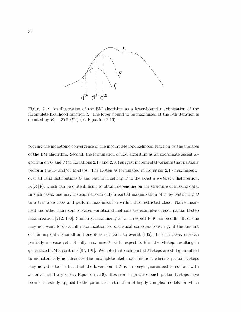
32
F1
(0) θ θ(1) (2)θ
L
F2
Figure 2.1: An illustration of the EM algorithm as a lower-bound maximization of theincomplete likelihood function L. The lower bound to be maximized at the i-th iteration isdenoted by Fi ≡ F(θ,Q(i)) (cf. Equation 2.16).
proving the monotonic convergence of the incomplete log-likelihood function by the updates
of the EM algorithm. Second, the formulation of EM algorithm as an coordinate ascent al-
gorithm on Q and θ (cf. Equations 2.15 and 2.16) suggest incremental variants that partially
perform the E- and/or M-steps. The E-step as formulated in Equation 2.15 maximizes F
over all valid distributions Q and results in setting Q to the exact a posteriori distribution,
pθ(X|Y), which can be quite difficult to obtain depending on the structure of missing data.
In such cases, one may instead perform only a partial maximization of F by restricting Q
to a tractable class and perform maximization within this restricted class. Naive mean-
field and other more sophisticated variational methods are examples of such partial E-step
maximization [212, 150]. Similarly, maximizing F with respect to θ can be difficult, or one
may not want to do a full maximization for statistical considerations, e.g. if the amount
of training data is small and one does not want to overfit [135]. In such cases, one can
partially increase yet not fully maximize F with respect to θ in the M-step, resulting in
generalized EM algorithms [87, 191]. We note that such partial M-steps are still guaranteed
to monotonically not decrease the incomplete likelihood function, whereas partial E-steps
may not, due to the fact that the lower bound F is no longer guaranteed to contact with
F for an arbitrary Q (cf. Equation 2.19). However, in practice, such partial E-steps have
been successfully applied to the parameter estimation of highly complex models for which
33
calculating the exact a posteriori distribution in Equation 2.17 is not feasible [119]. Third,
the EM updates are automatic, i.e. they are free of any learning rate or other parameters
requiring handtuning. Lastly, we under suitable regularity conditions the EM updates are
guaranteed to converge to a local maximum of the incomplete data likelihood function, and
the convergence rate around a local maximum is first order [87].
Overall, the EM algorithm is mathematically elegant and has a number of attractive
properties including monotonic convergence and being free of any handtuning parameters,
resulting in its popularity. It is one of the most widely used algorithms in statistics and
engineering, for example, it is regularly used for the ML parameter estimation of the HMM-
based large vocabulary speech recognizers involving millions of parameters [225, 273].
2.5 Exponential Family
The exponential family is an important class of parametric distributions with a rich math-
ematical structure, interplaying between statistics and convex analysis [20, 21]. The ex-
ponential family covers both discrete and continuous distributions and their hybrids. The
multinomial, Gaussian, Poisson and exponential distributions are a few well known members
of this family. The exponential family distributions also naturally emerge as solutions to
the maximum entropy problem [117]. Our work about discriminative and likelihood-based
parameter estimation in the exponential family in the later chapters will heavily use math-
ematical properties of exponential family, and our goal in this section is to review these.
Due to these properties, exponential family distributions have a number of attractive prop-
erties in parameter estimation such as accepting sufficient statistics and a unique maximum
likelihood estimate.
A probability distribution pθ(X) for X ∈ X in the exponential family takes the following
general form [55]:
pθ(X = x) ≡ c(x) exp{θ>t(x)− ψ(θ)
}, (2.20)
where c(x) determines the measure according to which pθ(x) is a distribution; θ ∈ Rd is
the d-dimensional parameter vector; t(x) is the sufficient statistics; and ψ(θ) is the log-

34
normalization constant ensuring that pθ(x) integrates to one:
ψ(θ) ≡ log(∫
c(x) exp{θ>t(x)
}dx
), (2.21)
where without loss of any generality we assumed that X is continuous valued. We note
that the dimensionality d of the sufficient statistics t(x) is in general different from (usually
higher than) the dimensionality of X. Exponential family distributions have many possible
parameterizations, and the parameters θ in the form in Equation 2.20 are often referred to
as natural parameters. The natural parameters θ are constrained such that θ ∈ Θ where
Θ ≡{θ ∈ Rd | ψ(θ) <∞
}, (2.22)
ensuring that the log-normalization constant ψ(θ) in Equation 2.21 is well defined. The
set Θ is convex due to the convexity of ψ(θ). Notice that the condition in Equation 2.22
does not place any constraints on θ, if the sample space is discrete but may restrict θ to a
strict subset of Rd for continuous sample spaces. A parameterization is called minimal if the
elements of θ and t(x) are linearly independent and called overcomplete otherwise. In the
following we will assume that all natural parameterizations θ are minimal, unless otherwise
noted. We will also be working in regular exponential families for which Θ is an open
set, without much restriction (multinomial Gaussian, multivariate Gaussian, Poisson, and
exponential distributions, among many others, are regular exponential families) [260, 55].
The log-normalization constant ψ(θ) plays a central role in the exponential family, and
here we will list a few of its key properties [55]. First, ψ(θ) is convex, and strictly convex
if the parameterization is minimal, the proof of which naturally comes out of the next
property. Second, the derivatives of ψ(θ) are equal to the cumulants of sufficient statistics
t(X). As a result, ψ(θ) is also often referred to as the cumulant-generating function. Under
suitable regularity conditions justifying the exchange of derivation and integration, one finds
by direct differentiation in Equation 2.21 that [260]
∂ψ(θ)∂θ
= E [t(X)] , (2.23)
∂2ψ(θ)∂θ ∂θ>
= cov [t(X)] . (2.24)
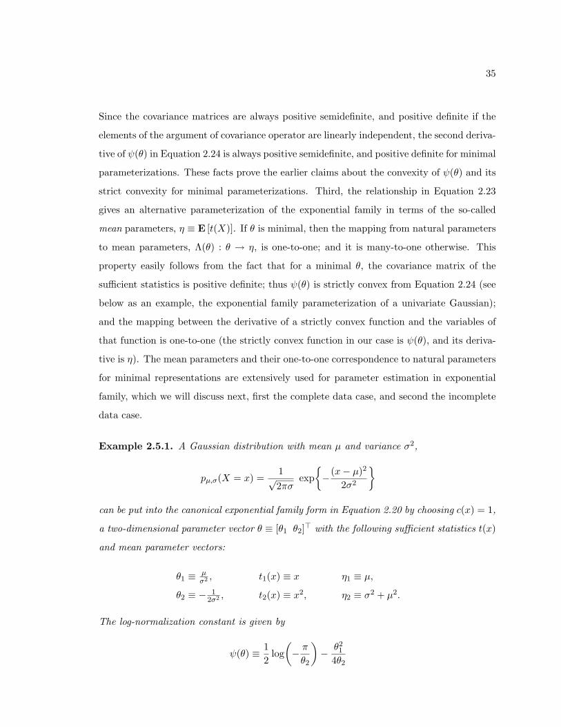
35
Since the covariance matrices are always positive semidefinite, and positive definite if the
elements of the argument of covariance operator are linearly independent, the second deriva-
tive of ψ(θ) in Equation 2.24 is always positive semidefinite, and positive definite for minimal
parameterizations. These facts prove the earlier claims about the convexity of ψ(θ) and its
strict convexity for minimal parameterizations. Third, the relationship in Equation 2.23
gives an alternative parameterization of the exponential family in terms of the so-called
mean parameters, η ≡ E [t(X)]. If θ is minimal, then the mapping from natural parameters
to mean parameters, Λ(θ) : θ → η, is one-to-one; and it is many-to-one otherwise. This
property easily follows from the fact that for a minimal θ, the covariance matrix of the
sufficient statistics is positive definite; thus ψ(θ) is strictly convex from Equation 2.24 (see
below as an example, the exponential family parameterization of a univariate Gaussian);
and the mapping between the derivative of a strictly convex function and the variables of
that function is one-to-one (the strictly convex function in our case is ψ(θ), and its deriva-
tive is η). The mean parameters and their one-to-one correspondence to natural parameters
for minimal representations are extensively used for parameter estimation in exponential
family, which we will discuss next, first the complete data case, and second the incomplete
data case.
Example 2.5.1. A Gaussian distribution with mean µ and variance σ2,
pµ,σ(X = x) =1√2πσ
exp{−(x− µ)2
2σ2
}can be put into the canonical exponential family form in Equation 2.20 by choosing c(x) = 1,
a two-dimensional parameter vector θ ≡ [θ1 θ2]> with the following sufficient statistics t(x)
and mean parameter vectors:
θ1 ≡ µσ2 , t1(x) ≡ x η1 ≡ µ,
θ2 ≡ − 12σ2 , t2(x) ≡ x2, η2 ≡ σ2 + µ2.
The log-normalization constant is given by
ψ(θ) ≡ 12
log(− πθ2
)− θ2
1
4θ2

36
which can be shown to be strictly convex by direct differentiation. Finally, the parameter set
Θ at which the integral of pµ,σ(X) converges is given by
Θ ≡{θ ∈ R2 | θ2 < 0
}.
2.5.1 Maximum Likelihood Estimation with Complete Data
Consider the maximum likelihood parameter estimation of a general exponential family
distribution in Equation 2.20, which we rewrite for convenience,
pθ(X = x) = c(x) exp{θ>t(x)− ψ(θ)
}. (2.25)
Given a complete data set X ≡ {X1, . . . , XN}, the maximum likelihood parameters θml are
found by maximizing the log-likelihood function:
θml ≡ argmaxθ∈Θ
{ N∑n=1
(log c(Xn) + θ>t(Xn)− ψ(θ)
)}. (2.26)
The parameter set Θ is convex set as well as the log-likelihood function in Equation 2.26.
Thus, the global maximum of the log-likelihood function in Equation 2.26, if it is achieved
at a point θ in Θ, can be found by taking derivatives and setting them to zero, yielding
ηml =1N
N∑n=1
t(Xn) (2.27)
where ηml denotes the mean parameters corresponding to the maximum likelihood esti-
mate θml, and we have used the invariance of maximum likelihood estimate to such re-
parameterizations. Hence, the maximum likelihood estimate, if it exists, is simply found by
setting the mean parameters η (defined as the expected sufficient statistics) to the empirical
mean of the sufficient statistics in the data. Notice that the maximum likelihood estimate
depends on data only through the sufficient statistics, which is the operational meaning of
sufficiency: θ and X depend on each other only via t(X).
The estimate in Equation 2.27 exists only if the empirical mean of the sufficient statistics
in the training data lies in the relative interior of the setM, riM, where
M≡{µ ∈ Rd
∣∣ ∃ p ∈ P s.t. Ep [t(X)] = µ}, (2.28)
37
the set consisting of all mean vectors that can be realized by some probability distribution p
that is absolutely continuous with respect to the measure c(x) dx for x ∈ X (the set P) [260].
The technical condition that (1N
N∑n=1
t(Xn))∈ riM
amounts to excluding singular covariance matrices for multivariate Gaussian distributions
or degenerate probability vectors with 0 or 1 elements for multinomial distributions. It is
almost always achieved in practice provided that the sample size N is large enough.
2.5.2 Maximum Likelihood Estimation with Incomplete Data
Now let us consider the case in which we want to estimate parameters θ of pθ(X) in Equa-
tion 2.25 from the incomplete sample Y ≡ {Y1, . . . , YN}, where Y ≡ h(X) for many-to-one
h(X). We denote the unavailable complete data by X ≡ {X1, . . . , XN}. (We assume for
simplicity that each example in our data set has the same missing data pattern.) As we
have seen in Section 2.4, the EM algorithm can be used for maximum likelihood parameter
estimation with incomplete data, and it takes a particularly simple form when applied in
the exponential family.
The general EM algorithm maximizes the following expected complete likelihood func-
tion at the i-th iteration (cf. Equation 2.18),
θ(i) ≡ argmaxθ∈Θ
{Eθ(i−1) [log pθ(X )|Y]} ,
which reduces to
θ(i) = argmaxθ∈Θ
{θ>( N∑
n=1
Eθ(i−1) [t(Xn)|Yn])−Nψ(θ)
}(2.29)
for the exponential family pθ in Equation 2.25. The EM algorithm’s objective function in
Equation 2.29 is exactly analogous to that for maximum likelihood estimation with complete
data in Equation 2.26, the only difference being that the replacement the sample mean
of complete data sufficient statistics in Equation 2.26 by its expected value conditional
on observed data in Equation 2.29. Repeating the same steps that we have applied for
38
obtaining the complete data maximum likelihood solution, we find that the EM algorithm
update in Equation 2.29 is found by setting [87]
η(i) ≡ 1N
N∑n=1
Eη(i−1) [t(Xn)|Yn] (2.30)
at the i-th iteration.
Overall, the EM algorithm’s solution in the incomplete data case is very similar to
the maximum likelihood solution in the complete data case and differs only in the use of
expected value of complete data sufficient statistics instead of using them directly (since they
are unavailable). Such expectations can usually be taken easily, as we will see in the next
section for hidden Markov models. However, we note that while the maximum solution in
Equation 2.27 for the complete data attains the global maximum of the likelihood function in
a single step, the updates of the EM algorithm in Equation 2.30 are guaranteed to converge
to only a local maximum of the incomplete likelihood function.
2.6 Hidden Markov Models
The samples or observations from temporal processes such as speech and machining vibra-
tions does not follow a fixed distribution over time and rather their statistics temporally
change depending on some underlying phenomenon such as the linguistic context in speech,
or the wear amount on cutting tools in machining. Moreover, the observations that are
near in time tend to be highly correlated. A hidden Markov model (HMM) is a dynamic
probabilistic model appropriate for characterizing such processes [224, 163, 213, 37].
An HMM consists of two parts: an observation sequence {Ot}T−1t=0 with length T and
an underlying state sequence {St}T−1t=0 . Observations can be discrete or continuous valued,
whereas the states are discrete valued with a finite sample space S ≡ {1, . . . , |S|}. States
represent the temporally changing characteristics of the process, and observations are emit-
ted from states. An HMM is a generative probabilistic model, and as such, it involves a
mechanism for the evolution of states over time and another one for characterizing obser-
vations given the underlying states. Without making any assumptions, we can decompose
the joint probability distribution of states and observations into two parts using the chain

39
2 31
Figure 2.2: A left-to-right state transition topology with three states, where only self-transitions or transitions to the next state are allowed.
rule of probability:
p({St}, {Ot}) = p({St}) p({Ot}|{St}). (2.31)
The HMM makes strong simplifying assumptions regarding how the evolution of states
p({St}) and the observational variability given states p({Ot}|{St}) are modeled.
The HMM characterizes the state evolution as a first-order Markov chain:
p({St}) ≡ p(S0)T−1∏t=1
p(St|St−1), (2.32)
in which p(S0) and p(St|St−1) specify initial state and state-transition, respectively, prob-
abilities. In this work we will assume that the state-transition distributions are time-
homogeneous. Usually some form of regularity in the structure of transitions is assumed,
such as a left-to-right topology where transitions only occur to higher-ordered states, see
Figure 2.2. At each time step, a new state is chosen conditional on the previous one from
the allowable state transitions in the state transition topology.
The HMM characterizes the observational variability conditional on hidden states by
assuming that observations are independent of each other given their respective states:
p({Ot}|{St}) ≡T−1∏t=0
p(Ot|St). (2.33)
The consecutive observations generated from the same state are i.i.d, but only condition-
ally so; and they are not marginally independent when the hidden states are marginalize
out. However, the conditional independence assumption in Equation 2.33 implies that any
dependencies among observations are mediated through hidden states.

40
S0
0O
S
O1
1 S
O
...T−1
T−1
Figure 2.3: An undirected graphical model illustration of the HMM, where state and obser-vation sequences are unfolded in time. The edges represent probabilistic dependencies. SeeSection 2.7 for the probabilistic interpretation of such graphs.
By plugging the parts in Equations 2.32 and 2.33 related to the state evolution and
observational variability, respectively, into Equation 2.31, we obtain the HMM factorization
of the joint distribution of the observation and state sequences:
p({St}, {Ot}) ≡ p(S0) p(O0|S0)T−1∏t=1
p(St|St−1) p(Ot|St). (2.34)
As compared to the factorization in Equation 2.31 which is always true, the HMM factoriza-
tion in Equation 2.34 entails two assumptions: the state sequence is first-order Markov, and
the observations are independent of everything else conditional on states. A graphical model
illustration of the HMM in Figure 2.3 clearly depicts these two independence assumptions
via the notion of vertex separation in graphs.
In many applications, states {St} are used for modeling purposes only and not observed.
Thus, they need to be marginalized out to make inferences using an HMM. First, the
marginal probability of the observations
p({Ot}) =∑{St}
p({St}, {Ot}) (2.35)
is of interest, for example, for finding the most likely class in a pattern classification problem
with the features X ≡ {Ot} where each class-conditional distribution p(X|C) is modeled as
an HMM (cf. Section 2.2). Second, the state a posteriori distribution,
p({St}|{Ot}) =p({St}, {Ot})p({Ot})
, (2.36)
is needed for answering queries about states, e.g. most possible hidden state completion, and
for maximum likelihood parameter estimation with the EM algorithm (cf. Section 2.6.3).
41
In addition, we will need the single and pairwise state posteriori probabilities, p(St|{Ot})
and p(St−1, St|{Ot}), respectively, in the EM algorithm, and they should also be efficiently
calculated. Third, it is of interest to find the most likely state sequence,
{s∗0, . . . , s
∗T−1
}≡ argmax
{s0,...,sT−1}{p(S0 = s0, . . . , ST−1 = st−1|{Ot})} , (2.37)
which might have generated the observation sequence {Ot}, for example, for decoding words
underlying an acoustic waveform in speech recognition. The brute force calculation of these
and other quantities by maximizing or summing over all state sequences in Equation 2.34
would require O(|S|T ) operations, which is prohibitive even for small |S|.
In the next three sections we will show how the inference and parameter estimation
problems of HMMs can be efficiently solved via the forward-backward, Viterbi, and Baum-
Welch algorithms. We will provide detailed derivations of these algorithms, as similar ideas
will be used in Chapter 4 for a multi-scale extension of HMMs.
2.6.1 The Forward-Backward Algorithm
In this section we will describe the forward-backward algorithm, an efficient method for cal-
culating the single and pairwise state a posteriori probabilities and the marginal probability
of observations [225, 224]. To efficiently calculate these quantities, the forward-backward
algorithm heavily exploits the two independence assumptions of HMMs: each observation
is independent of everything given its state, and the state sequence is a Markov chain. We
note that conditioning on the state at time t, St, renders the past and future observations,
{O0, . . . , Ot} and {Ot+1, . . . , OT−1}, respectively, independent of each other. Using this
property, we will express the single and pairwise state a posteriori probabilities in terms of
quantities that depend on only the past and the future variables and then provide recursions
to efficiently calculate these quantities.
We can decompose the state a posteriori probability p(St|{Ot}) as
p(St|{Ot}) ∝ p(St, O0, . . . , Ot) p(Ot+1, . . . , OT−1|St) (2.38)
where we used the aforementioned independence property. Similarly, we decompose the
42
pairwise state a posteriori probability p(St, St−1|{Ot}) as
p(St−1, St|{Ot}) ∝ p(St−1, O0, . . . , Ot−1) p(St|St−1) p(Ot|St)
× p(Ot+1, . . . , OT−1|St) (2.39)
again using the same independence property and the fact that conditioning on St renders
Ot independent of everything else. We see that decompositions in Equations 2.38 and 2.39
can be expressed in terms of the quantities p(St−1, O0, . . . , Ot−1) and p(St−1, O0, . . . , Ot−1)
(and a few others which are readily available). These quantities will play a central role in
the inference algorithm [225], so we give them special names:
αt(s) ≡ p(St = s,O0, . . . , Ot), (2.40)
βt(s) ≡ p(Ot+1, . . . , OT−1|St = s). (2.41)
With this newly defined notation, we rewrite p(St|{Ot}) and p(St−1, St|{Ot}) as
p(St|{Ot}) ∝ αt(St) βt(St), (2.42)
p(St−1, St|{Ot}) ∝ αt−1(St−1) p(St|St−1) p(Ot|St) βt(St). (2.43)
The normalization constants for the single and pairwise state a posteriori probabilities in
Equations 2.42 and 2.43 are equal to p({Ot}), and hence, the same for all t. We can obtain
p({Ot}) from αT−1(ST−1) using the definition in Equation 2.40:
p({Ot}) =∑s∈S
αT−1(ST−1 = s). (2.44)
As a result, all single and pairwise state a posteriori probabilities and the marginal prob-
ability of observations can be easily calculated once we have a way to efficiently calculate
{αt} and {βt}.
The {αt} can be calculated by a recursion forward in time [225]. We initialize the forward
recursion by setting
α0(s) = p(S0 = s) p(O0|S0 = s)
for s ∈ S, using the definition of αt in Equation 2.40 for t = 0. For t > 0, αt is obtained
from αt−1 as follows:
αt(s) =∑s′∈S
αt−1(s′) p(St = s|St−1 = s′
)p(Ot|St = s
). (2.45)
43
The recursion for βt similarly works but backward in time for t < T − 1:
βt(s) =∑s′∈S
p(St+1 = s′|St = s) p(Ot+1|St+1 = s′) βt+1(s′). (2.46)
The definition of βt in Equation 2.41 does not help us to initialize the backward recursion
at time T −1, but the choice βT−1(s) ≡ 1 works, as can be seen by comparing the definition
of βT−2(s) with the righthand side in Equation 2.46 for t = T − 2.
Overall, the forward and backward recursions in Equations 2.45 and 2.46, respectively,
in combination with Equations 2.42, 2.43, and 2.44 provides us a method to efficiently com-
pute all single and pairwise (consecutive) state a posteriori distributions and the marginal
probability of observations. The computational cost of the forward and backward recursions
are O(T |S|2), which is linear in the sequence length T instead of being exponential as in
the brute force method. Notice that the backward recursion is not necessary, if one is only
interested in the marginality of observations, in particular for decoding.
2.6.2 The Viterbi Algorithm
The Viterbi algorithm [225, 224] finds the most likely state sequence (cf. Equation 2.37) in
a way reminiscent of the forward recursion in Equation 2.45, by dynamic programming. In
effect, the only difference between the forward recursion and the Viterbi algorithm is the
replacement of the summation operator in the forward recursion by the maximum operator
in the Viterbi algorithm.
We define the probability of the most likely partial state sequence ending at a particular
state based on the partial sequence up to that point:
δt(s) ≡ max{s0,...,st−1}
{p(S0 = s0, . . . , St−1 = st−1, St = s,O0, . . . , Ot)} . (2.47)
The state sequence up to time t takes the state sequence sequence up to time (t − 1)
as a subsequence. Thus, the most likely partial state sequence ending at time t can be
obtained from the most likely state sequence ending at time t− 1 using Belman’s principle
of optimality [155]:
δt(St = s) ≡ maxs′
{δt−1
(St−1 = s′
)p(St = s|St−1 = s′
)p(Ot|St = s
)}, (2.48)

44
for t > 1. The recursion is started at time 0 using the definition in Equation 2.47. The
lefthand side in Equation 2.48 needs to calculated for all t and s, since we do not know
the most likely state sequence until we come to the very end. As such, it is also necessary
to keep track of the previous state from which we come to the optimal sequence ending at
state s at time t:
ψt(St = s) ≡ argmaxs′
{δt−1(St−1 = s′) p(St = s|St−1 = s′) p(Ot|St = s)
}.
After calculating δt(St = s) for all t and s, we find the optimal ending state by
s∗T−1 = argmaxs∈S
{δT−1(s)} ,
and using this ending point, we backtrack our steps to recover the elements of the Viterbi
state sequence for t = T − 2, . . . , 1:
s∗t = ψt+1(s∗t+1).
Overall computational cost of the Viterbi algorithm is O(T |S|2), and its memory re-
quirement is O(T |S|). We note that the Viterbi algorithm finds the most likely joint state
sequence (cf. Equation 2.37), not the single most likely state at a particular time. The
latter quantities can easily be obtained from the single state a posteriori probabilities in
Equation 2.42.
2.6.3 The Baum-Welch Algorithm
In this section, we will describe the Baum-Welch algorithm for maximum likelihood esti-
mation of HMMs. The main difficulty in the maximum likelihood estimation of HMMs is
due to the fact that states in an HMM are hidden. Similar to the other hidden variable
models, directly maximizing the incomplete likelihood function is difficult, and hence, we
resort to the EM algorithm (cf. Section 2.4). The parameter estimation of discrete HMMs
was originally formulated by Baum and his colleagues in the early 70’s [25, 26, 24], which
later turned out to be an instance of the general EM algorithm [87]. The EM algorithms
for discrete or continuous HMMs are commonly referred to as the Baum-Welch algorithm.
Here we will focus on HMMs with mixture of Gaussian output distributions, since this will
45
be the form that will be using in our applications, and our work in Chapter 4 about a
multi-scale extension of HMMs will also involve similar mixture distributions and the EM
algorithm for parameter estimation.
The parameters of an HMM with the mixture of Gaussian output distributions consist
of initial state probabilities, πs ≡ p(S0 = s), state-transition probabilities, ass′ ≡ p(St =
s|St−1 = s′), and mixture weights, means, and covariances, {κms, µms,Σms}, associated
with the Gaussian output distributions:
p(Ot = o|St = s) =M∑
m=1
αms N (o;µms,Σms) (2.49)
where N (·;µ,Σ) denotes a multivariate Gaussian distribution with the mean vector µ and
covariance matrix Σ:
N (o;µ,Σ) ≡ 1(2πd|Σ|)1/2
exp{−1
2(o− µ)>Σ−1(o− µ)
}
in which d is the dimensionality of observations, and |Σ| denotes the determinant of Σ. In
Equation 2.49, M is the number of mixture components, and αls, µms and Σms, are the
weight, mean vector, and covariance matrix, respectively, for the mixture component m in
state s. The mixture weights αms’s are such that∑
m αms = 1, for all s. We will collectively
denote all parameters in an HMM as θ.2
In our derivation, we will assume that there is only one observation sequence {Ot} in
the training data. The extension to the case with multiple observation sequences is simply
achieved by pooling the sufficient statistics from all sequences together in the re-estimation
equations below. To derive the EM algorithm for the HMM, we construct the auxiliary
2This θ is not to be confused with the θ in Section 2.5, denoting the natural parameters for the exponentialfamily. As an aside, we note that not all HMMs are in the exponential family, in particular those withleft-to-right state transition topologies due to zero probabilities assigned to some state combinations.However, such left-to-right and most other HMMs that are not in the exponential family, can be expressedas mixtures of exponential family distributions.

46
function in Equation 2.18 and simplify using the HMM factorization in Equation 2.34:
θ(i) ≡ argmaxθ
{Eθ(i−1)
[log p
({St}, {Ot}
)|{Ot}
]}= argmax
θ
{∑s∈S
γ0(s) log πs +∑
s,s′∈S
T−1∑t=1
ξt(s, s′) log ass′
+∑s∈S
T−1∑t=0
γt(s) log p(Ot|St)}
(2.50)
where
γt(s) ≡ pθ(i−1)(St = s|{Ot}),
ξt(s, s′) ≡ pθ(i−1)(St = s, St−1 = s′|{Ot}),
the single and pairwise, respectively, state a posteriori probabilities calculated according
to the parameters from the previous iteration using the forward-backward algorithm (cf.
Section 2.6.1). The expected likelihood function Equation 2.50 is separated into the terms
that only depend on the initial state, state transition, and output distributions. Maximizing
it with respect to πs and ass′ yields the following update equations for the initial state and
state transition probabilities:
π(i)s = γ0(s),
a(i)ss′ =
∑T−1t=1 ξt(s, s′)∑T−2t=0 .γt(s)
The maximization of the last term in Equation 2.50, related to the mixture of Gaussian
output distributions, can also be easily accomplished [32], yielding the following update
equations for the mixture weights, means and covariances:
α(i)ms =
∑T−1t=0 γt(m, s)∑Mi=1 γt(m, s)
(2.51)
µ(i)ms =
∑T−1t=0 γt(m, s) Ot∑T−1
t=0 γt(m, s)(2.52)
Σ(i)ms =
∑T−1t=0 γt(m, s) OtO
>t∑T−1
t=0 γt(s,m)− µ(i)
ms
[µ(i)
ms
]> (2.53)
where we have defined, with a slight abuse of notation, that
γt(m, s) ≡ pθ(i−1)
(Mt = m,St = s|{Ot}
)= γt(s) γt(m|s) (2.54)

47
where Mt denotes the hidden mixture variable at time t. and γt(m|s) ≡ pθ(i−1)(Mt =
m|St = s,Ot), the mixture a posteriori probability, calculated from the mixture model in
Equation 2.49 using Bayes rule.
The updates of the EM algorithm in Equations 2.51–2.53 constitute a relatively straight-
forward method for maximum likelihood parameter estimation of HMMs with mixture of
Gaussian output distributions. The EM algorithm is the most commonly used method for
training of current HMM-based speech recognizers involving millions of parameters [273,
224]. However, discriminative criteria such as minimum classification error [165, 164, 70],
and most notably, maximum conditional likelihood (also known as maximum mutual in-
formation estimation) [210, 256, 244, 267] are also popularly used in speech recognition.
An iterative method called extended Baum-Welch training for maximum conditional likeli-
hood estimation of discrete HMMs have been developed in [126], which is later adopted to
continuous HMMs with Gaussian output distributions by a discrete approximation to the
Gaussian distribution [210]. The extended Baum-Welch parameter updates for HMMs are
similar to the usual Baum-Welch updates, but the sufficient statistics used in the extended
updates (i.e. the numerator and denominator counts in Equations 2.51–2.53) also have con-
tributions coming from examples from other classes in the training data and not just from
those with the same class label as in the usual Baum-Welch training. The training examples
originating from the class whose parameters are being updated contribute positively to the
extended Baum-Welch sufficient statistics, whereas those from other classes contribute neg-
atively. As a result, the discriminative estimation methods in general are computationally
more expensive, but they are found to be very useful for improving recognition performance
in speech recognition [256, 244, 267]. We will investigate the extended Baum-Welch param-
eter updates in detail in Chapter 6, where a maximum conditional likelihood estimation
method for the general exponential family is developed.
2.7 Graphical Models
Graphical modeling is a framework for probabilistic model specification via graphs, where
vertices of the graph represent random variables of the model, and the edges between them

48
Z
X Y
Z
X Y
Z
X Y
Figure 2.4: Undirected (top graph) and directed graphical models (bottom graphs) definedover three variables.
represent probabilistic dependency relations [218, 160, 77]. While the graph in a graphical
model encodes the structural assumptions about the model via Markov independence as-
sumptions implied by the graph structure, the kernels over groups of variables defined with
respect to the graph numerally specify probabilities that are consistent with these properties.
As such, graphical modeling formalism achieves a separation of qualitative and quantitative
features of a probability distribution over a large number of variables. The use of graphs as
a modeling tool holds the key to the success of graphical models for the compact represen-
tation of large-dimensional probability distributions. Roughly speaking, graphical models
with dense graph dependency structures correspond to more complex models, whereas those
with sparser graphs correspond to less complex ones. As we will see, graphs are also useful
as a data structure for constructing efficient inference and estimation algorithms operating
on generic graphical models. Graphs provide a convenient visual interface for humans to
specify and efficiently compare probabilistic models and to incorporate prior knowledge into
the statistical modeling process. As examples, three simple graphical models, one over an
undirected graph and the others over directed graphs, are depicted in Figure 2.4.
We said before that a graphical model defines a multivariate probability distribution
via a graph, where vertices represent random variables, and edges represent probabilistic
dependency relationships. More correctly, missing edges in the graph imply conditional
independence properties in the resulting distribution. For example, in the undirected graph
in Figure 2.4, the missing edge between the vertices X and Y implies that X and Y are
independent of each other when conditioned on Z. These properties are only implied by the

49
graph structure and hold in every graphical model defined over that graph. The mechanism
through which such relationships are specified is the path separation in graphs. Two sets
of vertices in a graph are separated by a third group if all paths between the first two
sets are blocked by the third set. Then, for a graphical model, the path separation implies
that the random variables corresponding to the sets of separated vertices are conditionally
independent of each other given the random variables corresponding to the separator set.
What constitutes a blocked path, and how such conditional independence statements can be
converted into a useful form for specifying multivariate probability distributions depend on
the underlying graph semantics. There are many types of graphical models such as directed
graphical models (also known as Bayesian networks) with directed edges [218], undirected
graphical models (also known as Markov random fields) with undirected edges [30, 29], chain
graphs with directed and undirected edges [175, 231], ancestral graphical models [232], and
even, a given graph might have multiple probabilistic interpretations, as in [175] and [9] for
chain graphs. Only undirected and directed graphical modeling formulations are relevant to
our work, particularly the latter formulation, which we will use for model specification and
comparison throughout this thesis. Our interest in undirected graphical models only lies to
the extent that the undirected graphical model formulation is heavily used in the junction
tree algorithm for probabilistic inference in directed graphical models.
The organization of this section is as follows. We will first define our graph notation and
terminology. We will then introduce undirected and directed graphical modeling formalisms
and finish with the junction tree algorithm for probabilistic inference in generic undirected
and directed graphical models [76].
2.7.1 Notation and Terminology
Our graph notation and terminology in this section is largely based on [174], which should
be consulted for a thorough treatment and proofs.
A graph is denoted by G ≡ (V,E) is a pair with the vertex set V and the edge set E. An
edge is an ordered vertex pair with α, β ∈ V and α 6= β. An edge (α, β) ∈ E is undirected
if its opposite (β, α) is also in E, and otherwise it is directed. No self loops on vertices or
50
edges between groups of vertices are allowed according to our definition of an edge.
We will mainly deal with graphs with only directed or undirected edges and call them
directed and undirected, respectively, graphs (cf. Figure 2.4). An undirected graph is called
complete if there is an edge between every pair of vertices. A directed graph is called
complete, if its undirected version, obtained by dropping the directionality of all directed
edges arrows, is complete.
The subgraph GA ≡ (A,EA) obtained by only keeping the vertex subset, A, and edges
in between, EA ≡ A ∩ (V × V ), is called the vertex induced subgraph by A. A clique is a
vertex induced subgraph, which is maximal with respect to edge inclusion. We will denote
a clique by C and the collection of all cliques in a graph by C. (This is the only section
where we use the symbols C and C to denote cliques and clique sets, respectively, in a
graph, instead of class variables and training data class labels, respectively, in a pattern
classification problem.) A clique separator or simply separator is the intersection between
cliques that have a nonempty intersection in terms of vertices they include. We will denote
a clique separator by S and the collection of all clique separators in a graph by S.
A path of length n between vertices α and β is a sequence of distinct vertices (α0 =
α, . . . , αn = β) such that (αi−1, αi) ∈ E, or (αi, αi−1) ∈ E. A directed path is a path but
with the restriction that (αi−1, αi) ∈ E but (αi, αi−1) /∈ E. As such, a directed path cannot
go against the directed edges. An n-cycle is a path of length n with the same begin and
end points, α and β. A cycle in a directed graph is said to be directed if all arrows in the
cycle lie in the same direction. A chord is an edge between two non-consecutive vertices in
the cycle. An undirected graph is chordal or triangulated, if there are no n-cycles without a
chord.
The parents pa(α) and children ch(α) of a vertex α in a directed graph are all vertices
joined to α by a directed edge towards α and a directed edge away from α, respectively.
The descendants de(α) of the vertex α are all vertices that can be reached from α via a
path (which is necessarily directed). The non-descendants nd(α) of α are all vertices in a
graph except itself and its descendants.
In an undirected tree, there exists at most one path between any pair of vertices. In a
directed tree, each vertex has at most one parent.

51
We say that a set of random variables X is conditionally independent of another set Y
given another set Z (X⊥⊥Y |Z in shorthand), if
p(X = x, Y = y|Z = z) = p(X = z|Z = z) p(Y = y|Z = z) (2.55)
whenever p(Z = z) > 0, for all x, y, and z, where we do not necessarily require that X,
Y and Z be distinct. The conditional independence is intimately related to factorization
of probability distributions. It can be shown that the conditional independence statement
X⊥⊥Y |Z holds, if and only if the joint probability distribution of X, Y , and Z factorizes
into components that depend on only (X,Y ) and (Y, Z):
p(X = x, Y = y, Z = z) = h(X = x,Z = z) k(Y = y, Z = z) (2.56)
for some h and k, and again for all x, y, and z [174]. The above factorization is by no means
unique, and an obvious solution is given by Equation 2.55.
Given a graph G = (V,E), a graphical model over a collection of random variables X is
formulated by associating the vertices V with variables in X ≡ {Xα}α∈V . We denote the
subset of variables corresponding to the vertex set A ⊆ V by XA ≡ {Xα}α∈A. Due to the
one-to-one correspondence between variables and vertices, we will refer to the vertices and
the variables that they correspond to interchangeably. In a graphical model, such conditional
independence properties are implied, whenever the two vertex sets are separated from each
other by another vertex set. In the next two sections, we will introduce what we mean by
separation for the undirected and directed graphs and describe implications for graphical
models defined over such graphs.
2.7.2 Undirected Graphical Models
In undirected graphical models, we associate an undirected graph G = (V,E) with a col-
lection of random variables X ≡ {Xα}α∈V . The undirected edges E in G represent the
dependency relations among the components of X. More correctly, each missing edge in the
graph implies a conditional independence statement in the probability distribution defined
by that graphical model. Put another way, whenever two sets of vertices are separated by
a third set, then the random variables associated with the vertices in the first two sets are

52
independent of each other conditional on the variables in the third set. The separation
semantics of the undirected graphs is particularly simple: two sets of vertices A and B
are separated by the vertex set S, if every path between each pair of vertices in A and B
has to go through a vertex in S. Undirected graphical models translate vertex separation
in graphs into conditional independence in probability distributions by the global Markov
property. We say that a distribution p is globally Markov with respect to G, if XA⊥⊥XB|XS
whenever the vertex sets A and B are separated by the vertex set S.3 We will indicate a
distribution that is Markov with respect to a graph G by pG. For example, in the undirected
graphical model in Figure 2.4, it is implied that X and Y are independent of each other
given Z.
We know from Equation 2.56 that conditional independence is intimately related to
factorization of probability distributions, so is the conditional independence in undirected
graphical models. A distribution pG is said to factorize with respect to the undirected graph
G, if it is of the form
pG(X) =1Z
∏C∈C
ψC(XC) (2.57)
where C denotes the cliques of G; ψC is the potential function associated with the clique C;
and, Z is a global normalization constant which we assume to be unity from here on, as it
can be absorbed into a clique potential potential. We require that ψC be nonnegative but
arbitrary otherwise. Notice that there is also some arbitrariness in the joint specification
of ψC ’s according to Equation 2.57. It can be shown that for every pG of the form in
Equation 2.57, the global Markov property with respect to G holds, justifying the notation
pG. However, the converse is not true in general, i.e. there are distributions that do not
factorize with respect to G but still obey the global Markov property, but for continuous
and positive distributions, the Hammersley-Clifford theorem shows that the converse also
holds [137].
In general, the potential functions, ψC(XC)’s, in Equation 2.57 are not equal to the clique
marginals, but an important exception is the factorization with respect to decomposable
3Notice that the global Markov property only implies the conditional independence relationships that needto hold in p as implied by the graph structure and does not require that the graph faithfully representsall such relationships that hold in p. The latter requirement is more stringent than the former one.

53
graphs which are the undirected graphs that are triangulated [174]. For a decomposable
graph G, the potential functions can be chosen to be equal to the clique marginals:
pG(X) =∏
C∈C p(XC)∏S∈S p(XS)
(2.58)
where S denotes the clique separators of G. The factorization in Equation 2.58 in terms of
both clique and their separators can be put into the form in Equation 2.57 by arbitrarily
assigning each separator probability factor into one of the cliques that they are subsumed
by.
The undirected factorization in Equation 2.57 in terms of clique potentials plays a cen-
tral role in the parameter estimation and probabilistic inference of undirected graphical
models. We note that the clique potentials are in general coupled to each other via the
normalization constant Z in Equation 2.57, and their maximum likelihood estimation for
a generic undirected graphical model cannot be analytically performed even in the case
where no hidden variables are involved (except for decomposable models [174, 264]). How-
ever, a practical, coordinate-ascent algorithm, iterative proportional fitting, over the clique
potentials is available for their maximum likelihood estimation [79, 82, 85]. Probabilis-
tic inference in undirected graphical models is performed via the junction tree algorithm,
a common inference routine for undirected and directed graphical models, which we will
review in Section 2.7.4.
An HMM with the state and observation sequences, {St}T−1t=0 and {Ot}T−1
t=0 , respectively,
can be represented as an undirected graphical model (see Figure 2.3 for an undirected graph-
ical model representation of an HMM). The cliques of the HMM graph are the consecutive
state pairs {(St−1, St)}T−1t=1 and the state-observation pairs {(St, Ot)}T−1
t=0 , and the clique
separators of the HMM graph are the individual states {(St)}T−1t=0 . The HMM graph in
Figure 2.3 is trivially triangulated since it does not involve any cycles; it is decomposable;
and, its joint distribution can be factored in terms of the clique and separator marginal
probabilities as in Equation 2.58:
p({St}, {Ot}) =p(S0, S1) p(S0, O0)
p(S0)
(T−2∏t=1
p(St, St+1) p(St, Ot)p(St)2
)p(ST−1, OT−1)
p(ST−1). (2.59)
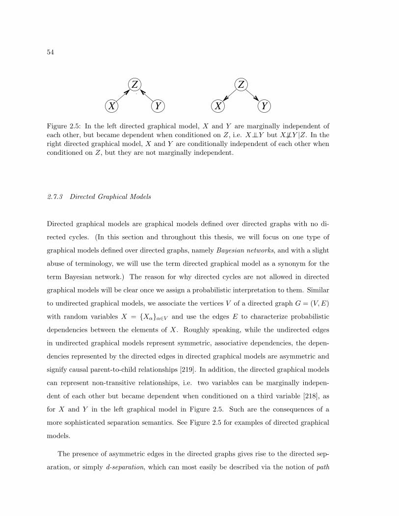
54
Z
X Y
Z
X Y
Figure 2.5: In the left directed graphical model, X and Y are marginally independent ofeach other, but became dependent when conditioned on Z, i.e. X⊥⊥Y but X 6⊥⊥Y |Z. In theright directed graphical model, X and Y are conditionally independent of each other whenconditioned on Z, but they are not marginally independent.
2.7.3 Directed Graphical Models
Directed graphical models are graphical models defined over directed graphs with no di-
rected cycles. (In this section and throughout this thesis, we will focus on one type of
graphical models defined over directed graphs, namely Bayesian networks, and with a slight
abuse of terminology, we will use the term directed graphical model as a synonym for the
term Bayesian network.) The reason for why directed cycles are not allowed in directed
graphical models will be clear once we assign a probabilistic interpretation to them. Similar
to undirected graphical models, we associate the vertices V of a directed graph G = (V,E)
with random variables X = {Xα}α∈V and use the edges E to characterize probabilistic
dependencies between the elements of X. Roughly speaking, while the undirected edges
in undirected graphical models represent symmetric, associative dependencies, the depen-
dencies represented by the directed edges in directed graphical models are asymmetric and
signify causal parent-to-child relationships [219]. In addition, the directed graphical models
can represent non-transitive relationships, i.e. two variables can be marginally indepen-
dent of each other but became dependent when conditioned on a third variable [218], as
for X and Y in the left graphical model in Figure 2.5. Such are the consequences of a
more sophisticated separation semantics. See Figure 2.5 for examples of directed graphical
models.
The presence of asymmetric edges in the directed graphs gives rise to the directed sep-
aration, or simply d-separation, which can most easily be described via the notion of path

55
blocking. A path4 from the vertex α to β in a directed graph is said to be blocked by the
vertex set S, if S contains a vertex γ satisfying either of the following two conditions [218]:
• The vertex γ is in S, and the arrows do not meet tail-to-tail at γ (→ γ ←); or,
• Neither γ nor any of its descendants is in S, and the arrows meet tail-to-tail at γ.
A path can become blocked or active, i.e. not blocked, depending on the configuration the
variables that might not be even on the path. The two vertices α and β are separated by
the vertex set S, if all paths between the two are blocked by S. Similarly, the vertex sets A
and B are separated by the subset S, if each pair of vertices in A and B are separated by
S. In directed graphical models, such path separation properties translate into conditional
statements among the corresponding random variables: XA⊥⊥XB|XS .
All conditional independence statements encoded by a directed graph can be collected
under the directed global Markov property [174]. A distribution p(X), X = {Xα}α∈V , is
said to obey the directed global Markov property with respect to the directed graph G,
if XA⊥⊥XB|XS whenever S d-separates A and B in G. It is a remarkable property of
the directed graphical models that such a global property can be shown to be equivalent
to a local one, directed local Markov property that is, each variable is independent of its
non-descendants given its parents [174]
Xα⊥⊥Xnd(α)|Xpa(α). (2.60)
For example, X and Y in the left directed graphical model in Figure are independent due
to the above directed local Markov property 2.5.
Let us consider an ordering of the vertices V such that each variable appears after its
parents, called a well-ordering or topological ordering. A well-ordering always exists [77].
Using a well-ordering of vertices and the local Markov property in Equation 2.60, we can
recursively factorize a distribution pG that is locally or globally Markov with respect to the
graph G, as follows:
pG(X) =∏α∈V
p(Xα|Xpa(α)), (2.61)
4We remind the reader that a path can go against the direction of arrows (cf. Section 2.7.1).
56
which is called the directed factorization property. If we were to factorize pG according to
an ordering which is not topological, then the resulting factorization would not necessarily
be as sparse. Thus, a suitable ordering of vertices could be crucial for inferring models from
data. In addition, we note that the chain rule of probability which is true for any p is a
special case of the directed factorization in Equation 2.61, as any p is Markov with respect
to a complete graph (no two vertices are d-separated in a complete graph, and hence, no
conditional independence relationship is implied). The global and local Markov properties
and the directed factorization property in directed graphical models are equivalent without
any restriction on the random variable collection X or the probability distribution p. In
addition, the directed factorization property clarifies why directed cycles are not allowed.5
While the undirected and directed graphical models share the same inference routine, the
junction tree algorithm, the maximum likelihood parameter estimation of directed graphical
models is considerably easier. If the parameters θα associated with each parent-to-child
conditional probability distribution p(Xα|Xpa(α)) in Equation 2.61 are independent of each
other, and the graphical model is completely observable, then the corresponding likelihood
function decomposes into vertex-dependent terms and parameters associated with vertex
can be separately estimated [66]. If there are hidden variables involved, the EM algorithm
can be used. In an EM algorithm for a directed graphical model, similar to the completely
observable case, the M-step (cf. Equation 2.16) is separately performed for each vertex-
dependent term, and the E-step consists of calculation of a posteriori probabilities over
hidden variables using, for example, the junction tree algorithm.
A directed model can be transformed into an undirected one through a procedure called
moralization, by adding undirected edges between all co-parents which are not connected
and dropping the directionality of arrows. Then, a pG factorizing with respect to the di-
rected graph G also factorizes with respect to its moral graph Gm, because each vertex
and its parents in G constitute a complete subset in the moralized graph Gm. However,
5If the directed cycles were allowed in a directed graphical model, the resulting factorization wouldnot correspond to a valid probability distribution for an arbitrary choice of parent-to-child conditionalprobability distributions. For example, in a two-vertex graphical model with a cycle between vertices1 and 2, the factorized distribution p(x1, x2) ≡ p1|2(x1|x2)p2|1(x2|x1) is not, in general, a probabilitydistribution for arbitrary but valid distributions p1|2 and p2|1 [54].
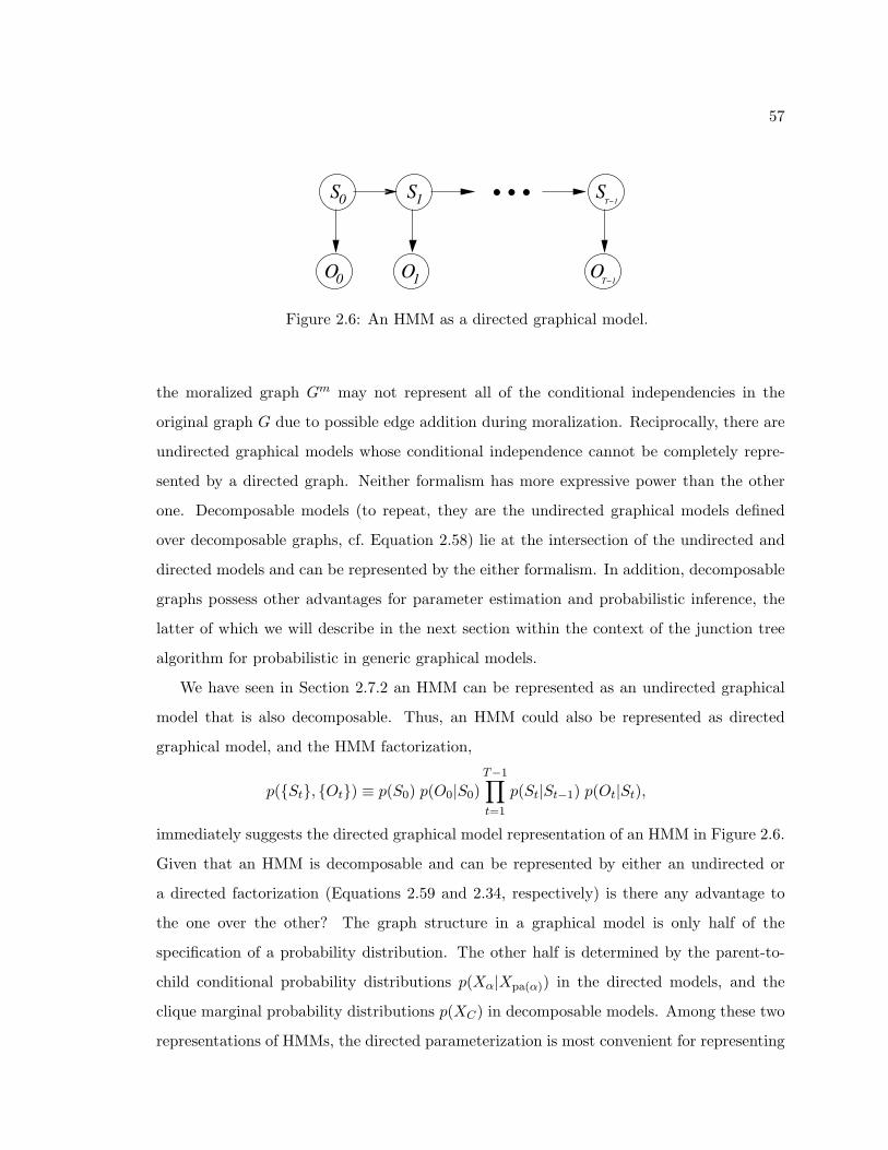
57
S0
0O
S
O1
1 S
O
...T−1
T−1
Figure 2.6: An HMM as a directed graphical model.
the moralized graph Gm may not represent all of the conditional independencies in the
original graph G due to possible edge addition during moralization. Reciprocally, there are
undirected graphical models whose conditional independence cannot be completely repre-
sented by a directed graph. Neither formalism has more expressive power than the other
one. Decomposable models (to repeat, they are the undirected graphical models defined
over decomposable graphs, cf. Equation 2.58) lie at the intersection of the undirected and
directed models and can be represented by the either formalism. In addition, decomposable
graphs possess other advantages for parameter estimation and probabilistic inference, the
latter of which we will describe in the next section within the context of the junction tree
algorithm for probabilistic in generic graphical models.
We have seen in Section 2.7.2 an HMM can be represented as an undirected graphical
model that is also decomposable. Thus, an HMM could also be represented as directed
graphical model, and the HMM factorization,
p({St}, {Ot}) ≡ p(S0) p(O0|S0)T−1∏t=1
p(St|St−1) p(Ot|St),
immediately suggests the directed graphical model representation of an HMM in Figure 2.6.
Given that an HMM is decomposable and can be represented by either an undirected or
a directed factorization (Equations 2.59 and 2.34, respectively) is there any advantage to
the one over the other? The graph structure in a graphical model is only half of the
specification of a probability distribution. The other half is determined by the parent-to-
child conditional probability distributions p(Xα|Xpa(α)) in the directed models, and the
clique marginal probability distributions p(XC) in decomposable models. Among these two
representations of HMMs, the directed parameterization is most convenient for representing
58
HMMs with time-homogeneous state transitions, because the directed representation of
HMMs in Equation 2.34 is directly defined in terms of state transitions p(St|St−1)’s. On the
other hand, marginal probabilities for single and pairwise states, p(St)’s and p(St−1, St)’s
in the undirected representation Equation 2.59 are algebraically coupled to each other for a
time-homogeneous Markov chain. As a result, parameter estimation of a time-homogeneous
Markov chain via undirected parameterization is rather cumbersome (yet straightforward),
and the directed model formulation seems more convenient to work with.
2.7.4 Junction Tree Algorithm
The junction tree algorithm is an efficient exact inference algorithm for general directed
and undirected graphical models [77, 160, 76]. In typical applications of graphical models,
only some of the variables in the model are observed, and the others remain hidden. The
term probabilistic inference refers to, among other things, calculation of the marginal prob-
abilities of observed variables and the a posteriori probabilities and modes (the most-likely
configurations) of hidden variables given the observed ones. In Section 2.6, we have seen
that these problems are efficiently solved for HMMs by exploiting the independence as-
sumptions of HMMs in the forward-backward and the Viterbi algorithms (cf. Sections 2.6.1
and 2.6.2, respectively). The junction tree algorithm works similarly but for general directed
and undirected graphs. In the junction tree algorithm, one compiles the original graph into
a clique-tree data structure, and then performs local message passing operations over this
structure. In this section, we will review the junction tree algorithm for the directed mod-
els,6 as it will be used for probabilistic inference of the models beyond HMMs of this thesis.
The kind of probabilistic inference we will be interested in is the inference in a directed
graphical model with hidden variables, where queries about hidden and observed variables
need to be answered given a configuration of observed variables.
The basic idea behind the junction tree algorithm is to convert the directed graphical
model into a decomposable one and then adjust the directed model parent-to-child condi-
tional probabilities in the directed factorization of Equation 2.61 to arrive at the decompos-
6The undirected case is identical except that the first step, in which a directed graph is converted into aundirected one, is omitted.
59
able graph factorization in Equation 2.58 in terms of clique and separator marginals. Once
this conversion is obtained, one can easily compute marginal probabilities for the observed
variables, or the a posteriori probabilities and the most likely configurations for the hidden
variables.
To convert a directed graph into a decomposable graph, we first transform it to an
undirected graph by moralization and then in turn transform this undirected graph into
a decomposable graph by triangulation. A directed graph is moralized by connecting all
co-parents which are not joined and dropping the directionality of arrows. As such, moral-
ization is unique. However, triangulation of an undirected graph where enough many edges
are added to the moralized graph so that there are no chordless cycles is trivially not unique.
Moralization and triangulation completes the graph operations necessary for converting the
directed graph into a decomposable graph. Notice that during this process, edges can only
be added and not deleted, and the directionality of arrows in the original graph is dropped.
As such, the path separation properties encoded in the resulting decomposable graph are a
subset of those in the original directed graph, and a probability distribution that is Markov
with respect to the original directed graph is necessarily Markov with respect to the re-
sulting undirected one, and we can obtain an undirected factorization with respect to the
resulting decomposable graph in terms of clique and separator potentials as follows. We set
all separator potentials to unity; and initialize all clique potentials to unity and then absorb
each parent-to-child conditional distribution by multiplication into a clique potential such
that the corresponding child and its parents live in that clique. At this stage, we have a
factorization over the decomposable graph, but the clique and separator potentials are not
equal to the clique and separator, respectively, marginals. The last step of the junction
tree algorithm is a local message passing procedure (similar to the forward and backward
recursion in the forward-backward algorithm of HMMs) between the neighboring cliques of
the triangulated graph to achieve such an equality. The message passing procedure modi-
fies the clique and separator potentials so that the clique and separator potentials become
equal to the corresponding marginal distributions, while preserving the global joint distri-
bution over the whole graph. The message passing is performed according to a protocol
on a junction tree, which is a spanning tree over the cliques with the running intersection

60
property that if a vertex appears in two cliques, then it appears in every clique along the
path joining these two cliques in the clique tree [174]. The running intersection property
is essential for achieving global consistency by locally passing messages between cliques.
Depending on the type of messages exchanged, one can obtain either the marginal and a
posteriori probabilities for observed and hidden, respectively, variables, or the Viterbi (i.e.
most likely) configurations and probabilities for hidden variables. For a full description of
the junction tree algorithm and why it is correct, see, e.g. [160, 163]. For a running example
of the junction tree algorithm, see Figure 2.7.
To summarize, the junction tree algorithm consists of following steps [76]:
1. Add an undirected edge between co-parents which are not joined, and drop the direc-
tionality of arrows (moralization);
2. Add undirected edges to the moralized graph until there are no chordless cycles (tri-
angulation);
3. Find the cliques of the triangulated graph and organize them as a clique tree having
the running intersection property; and,
4. Perform a message passing procedure on the junction tree.
The computational cost of the junction tree algorithm is determined by the size of the
messages passed between the cliques, which is in turn determined by the total clique state-
space cardinality. Even though the moralization of a directed graph is unique, there are
potentially many different triangulations and junction trees for an undirected graph [10,
169]. Moreover, there is usually some flexibility associated with the assignments of the
parent-to-child conditional probabilities to the clique potentials after the moralization and
triangulation steps [22]. The choice of the triangulation, junction tree and clique potential
assignments can have a large impact on the computational efficiency of the junction tree
algorithm, and for best performance, these operations need to be optimized [22]. However,
dense graphs corresponding to complex models necessarily have large cliques, for which
the practical use of the junction tree algorithm could be limited, and one may need to
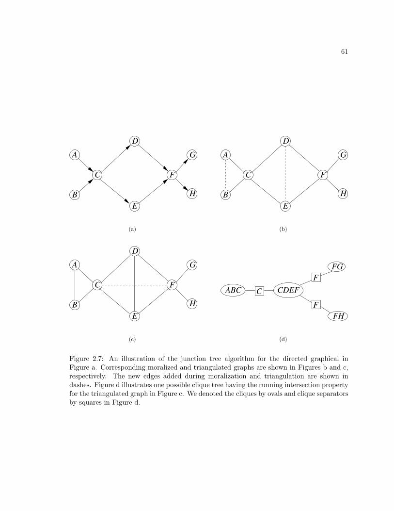
61
A
B
C
D
E
F
G
H
(a)
A
B
C
D
E
F
G
H
(b)
A
B
C
D
E
F
G
H
(c)
ABC CDEFF
FG
FFH
C
(d)
Figure 2.7: An illustration of the junction tree algorithm for the directed graphical inFigure a. Corresponding moralized and triangulated graphs are shown in Figures b and c,respectively. The new edges added during moralization and triangulation are shown indashes. Figure d illustrates one possible clique tree having the running intersection propertyfor the triangulated graph in Figure c. We denoted the cliques by ovals and clique separatorsby squares in Figure d.
62
resort to approximate inference techniques such as variational methods [161], or loopy belief
propagation [272].
2.8 Model Selection
In almost any application involving statistical modeling from data, in particular statistical
pattern recognition, our scientific knowledge of the underlying physical phenomenon is lim-
ited, and hence, we rarely know exactly which model (i.e. classifier in pattern classification)
to use. There are usually a set of hypotheses which are determined based on a variety of
criteria such as prior knowledge, mathematical tractability, and computational feasibility.
Model selection refers to a data-driven choice among competing models in the absence of
any prior knowledge in favor of one model against the others. We assume no prior knowledge
other than that for constructing hypotheses, and under this assumption, no universal learn-
ing algorithm that is uniformly superior to any other method for any application exists (no
free lunch theorem [92]). As such, we need a scientific principle for comparing models, and
in almost all model selection algorithms, this principle is the preference for simple theories,
the so-called Occam’s razor [186]. The main motivation for this simplicity principle comes
from the fact that simple models are more likely to generalize to unseen data than the more
elaborate ones. As we will see shortly, there are a variety model selection criteria proposed
based on this principle. The problem of model selection is not confined to pattern classifi-
cation, but rather it appears in any task involving statistical data modeling, e.g. regression
and estimation. In this section, we will discuss model selection first from a general data
modeling perspective and then address particular issues pertaining to pattern classification.
Graphical modeling formalism is particularly appropriate for model comparison and search,
and we will pay special attention to the model selection for the directed graphical models.
Let us consider the following generic data modeling problem. We want to infer a prob-
ability distribution p from a data set of i.i.d samples of size N , X ≡ {X1, . . . , XN}. For
the time being, we leave aside the ultimate use of the inferred model p, e.g. classification
or regression, but we will latter focus on classification. In inferring p from X , two levels
of inference can be distinguished. At the first level, we assume a particular model for p
63
and estimate its free parameters from data according to maximum likelihood, or some other
criteria. At the second level, we want to find out the best model among the hypotheses for
p [186]. This second level of inference is the model selection, and it concerns with any struc-
tural assumptions regarding the choice of p, whereas the first level of inference is concerned
with finding the optimal point within the assumed class of distributions. As such, the first
level of inference appears as a subroutine for the second level of inference. For parametric
modeling (as we will focus on), the first level of inference is parameter estimation as we
covered in Section 2.3. The second level of inference in parametric modeling concerns with
the choice of parametric family such as the diagonal vs. full covariance modeling in a multi-
variate Gaussian distribution, the number of mixture components of a mixture of Gaussians
model, or the graph dependency structure in a graphical model.
The fundamental problem in model selection is how to compare models with increasing
levels of complexity in terms of the number of their free parameters. Given two parametric
models H0 and H1, where H1 is a supermodel of H0, when should we prefer the more
complex H1 over the simpler H0? Suppose that we estimate parameters of each model
according to maximum likelihood criterion, which is reasonable given that our aim, for the
time being, is modeling data. Let us call the resulting likelihood of data for the i-th model
by p(X|Hi, θ
iml(X )
), θi
ml(X ) denoting the corresponding maximum likelihood estimate. The
comparison of the likelihoods p(X|H0, θ
0ml
)and p
(X|H1, θ
1ml
)does not directly reveal any
preference for one model against the other, since under the ML estimation paradigm, H1
always gives a higher likelihood than any of its sub-models, in particular H0. More complex
models can always fit the data better, i.e. have higher likelihoods, but they do not necessarily
generalize to unseen data. On the other hand, models with little modeling power might not
be sufficient for representing X and learning any interesting structure from data.
An insight into how generalization to unseen data depends on model complexity can be
gained from a bias-variance decomposition of the generalization error in regression using the
mean-squared error, but the conclusions are much more general. Suppose that we estimate
an unknown function f(x) by the regression g(x;X ), which is random in X with distribution

64
pX .7 It can be shown that the mean-squared error at a particular point x, averaged over
data sets X of the same size can be decomposed as follows [116]:
EpX (f(x)− g(x;X ))2 = (f(x)−EpX g(x;X ))2 + varpX g(x;X ) (2.62)
where the first term on the righthand side is the squared bias of the estimate g(x;X ), and
the second term is its variance. Complex models can significantly reduce the bias term,
but they also tend to have large variance due to the fact that they can overfit to the noise
in the data, and their estimates g(x;X ) can show a large variation across samples. For
a very complex model, the variance dominates the bias, resulting in high generalization
error. Thus, given two models which explain the training data equally well, one should
prefer the simpler model over the more complex one, since it is likely to have a lower
variance while having similar bias, and it can better generalize. This reasoning essentially
gives a quantification of Occam’s razor from a frequentist perspective (we will see another
interpretation of Occam’s razor from Bayesian perspective in Section 2.8.4). For a given
training data size, there usually exists an optimal balance between the estimation bias and
variance achieving the lowest generalization error, and finding the model with complexity
achieving this balance is the goal of model selection [116, 45].
There are a variety of criteria proposed in the literature for evaluating the fit to data
for model selection. As we will first focus on generic data modeling, we will evaluate the
fit to data by likelihood. A complex model always gives a higher likelihood than a simpler
one, and a direct comparison of likelihoods from different models does not take into account
the fact that their parameters are estimated on the same data set and the variance of
point estimation. There are a number of solutions proposed for meaningful comparison of
likelihoods by taking the model complexity into account. An obvious solution is to compare
the likelihoods on a different data set, which is the cross-validation solution. The likelihood-
ratio tests and penalized likelihood methods such as minimum description length penalizes
models according to their number of free parameters. On the other hand, the Bayesian
estimation framework avoids point estimates and provides an autonomous mechanism for
7The distribution pX is given by pX (X1, . . . , XN ) ≡QN
i=1 pX(Xi), assuming i.i.d. samples from thedistribution pX .
65
incorporating Occam’s razor. We will review these four solutions then focus on a particular
type of model selection problem, graph dependency structure selection for directed graphical
models, and finish with a discussion of model selection for pattern classification and specific
issues involved there.
2.8.1 Cross-validation
In leave-one-out cross-validation, we first train a model using all training samples but one,
say the l-th, X−l ≡ {X1, . . . , Xl−1, Xl+1, XN}, and use the estimated model to predict the
omitted sample, p(Xl|H, θml(D−l)). We then repeat this procedure for all samples and
obtain the cross-validation likelihood score [142]:
CV (X ,H) ≡N∑
n=1
log p(Xl|H, θml(X−l)
),
according to which models are compared. Cross-validation avoids the problem of double
inference on the same data set to some extent, but it is costly due to the fact multiple
models need to be estimated.
2.8.2 Likelihood-Ratio Testing
The most common solution to model selection in the mainstream statistics is the likelihood-
ratio testing. A likelihood-ratio test is a statistical test of goodness-of-fit between models
which are hierarchically nested [43]. A more complex model always gives a higher likelihood
than a simpler one, but the likelihood increase might not be justifiable in terms of the
additional number of parameters in the more complex model. The likelihood-ratio tests
provide an objective function for quantification of the significance of the likelihood increase.
Suppose that we want to test the hypothesis H1 against the null hypothesis H0, which is a
submodel of H1. First, we construct the likelihood-ratio test statistic based on the sample
X = x [31],
λ(x) ≡p(X = x|H0, θ
0ml(x)
)p(X = x|H1, θ1
ml(x)) ,
66
which is always less than or equal to unity. Next, we evaluate the probability of λ(X ) being
as extreme as the observed statistics λ(x) under the null hypothesis H0:
p ≡ pX(λ(X ) ≤ λ(x)|H0, θ
0ml(x)
), (2.63)
small values of which provide evidence against the null hypothesis H0, and we reject it at
the significance level α, if p < α. The typical significance values used in practice are 0.05 or
0.01. The calculation of the exact p-value in Equation 2.63 can be difficult, but, for large
sample sizes, it can be approximated by
p(χ2r ≥ −2 log λ(x))
where r is the number of additional parameters in H1 over H0, and χ2r denotes a chi-squared
random variable with r degrees of freedom [31, 264].
2.8.3 Minimum Description Length
A conceptually different view of model complexity is provided by the minimum description
length (MDL) principle [233]. Consider the following thought experiment. We want to
transmit the data X to a receiver over a communication channel using the shortest message
possible. We could directly transmit the data itself by using a fixed coding scheme, but the
statistical regularities in the source that generated X can be used to considerably reduce
the message length by using a code in which the shorter codewords are allocated to the
most likely sequences and the longer codewords to the unlikely ones. To construct such a
code, we need a probabilistic model of the source, for which we can use a model H that
we have inferred from the data X . Given H, we can use the following two-stage coding
scheme to transmit X . First we transmit the model H to the sender and then transmit the
codeword for X in the code based on H. Since the receiver has received the model H and
hence knows the code, it can decode the codeword that we sent for X to recover the data
X . Overall, the total message length that we used to transmit X is the sum of that for the
data X , L(X|H), and that for the model H, L(H):
description length = L(X|H) + L(H).

67
Let us now quantify these two message lengths.
In information theory, the optimal number of bits necessary for encoding a discrete
sample x ∈ X with distribution p is given by − log2 p(x) bits. Thus, in the code constructed
for X as if H were to the true distribution, the message length for X is − log2 p(X|H), which
is optimal, if H is actually the true generating distribution. For continuous X , the precision
δX at which X is specified is immaterial for model comparison purposes, as the message
length for recovering X at precision δX would be − log2(δX · p(X|H)), which differs from
− log2 p(X|H) by a constant for any model H.
Encoding the model H is more cumbersome [134], but for models that live in the same
superfamily such as Gaussian covariance models, the message lengths for alternative models
differ only in the number of bits needed to specify their nonzero parameters and which pa-
rameters are nonzero. We assume that parameters are continuous valued. We noted before
that the precision at which the continuous data is encoded is immaterial for model compar-
ison purposes, but the precision at which the parameters are specified obviously matters.
Under the model correctness assumption, the standard derivation of the maximum likeli-
hood estimate of a parameter is asymptotically proportional to 1/√N , as such specifying
the parameters only up to this precision can be justified [31]. Thus, the model description
length is equal to, up to an irrelevant constant,
L(H) = −k2
log2N
where k is the total number of parameters of the model H.
Putting together the description lengths of the model and the data given model, we find
that the total number of bits in the two-stage coding scheme to encode the data X is given
by [45]
description length = − log2 p(X|H, θml)−k
2log2 T . (2.64)
(To be strict, we should use the discretized parameters in the calculating likelihood above,
but for smooth likelihood functions, the approximation is justified.) We can see that the
description length that we arrived above is essentially the likelihood function with a penalty
term and offers a objective function for comparing alternative model hypotheses. In practice,

68
the penalty term is often multiplied by a “tweak” factor to get good results, especially if
comparing different kinds of structural changes such as covariance structure vs. number of
mixture components in a Gaussian mixture model.
The description length in Equation 2.64 has a strong flavor of Occam’s razor. Complex
models can reduce the first term on the righthand side of Equation 2.64 with their higher
likelihoods, but they also incur a penalty for their high number of parameters via the second
term, and vice versa for the simpler models. The optimal model according to the minimum
description length principle is the one that strikes a balance between its complexity and
accuracy of predictions.
The MDL principle is identical to the Bayesian information criterion [245], even though
the latter is derived as an asymptotic approximation to the Bayesian integrated log-likelihood
or the evidence, which we will define in the next section. The MDL is also similar to the
Akaike information criterion [92] in form, which is derived from yet different considerations
but differs from the description length in Equation 2.64 only in the complexity penalty term.
2.8.4 Bayesian Model Selection
We have noted before that there are two levels of inference in estimating a probability distri-
bution from data. At the first level, we fit a chosen model to data (parameter estimation),
and at the second level, we compare alternative model hypotheses (model selection) [186].
Up to now, we have focused on maximum likelihood methods which try to find the single
most likely setting of parameters at the first level of inference and compares models based on
this setting of parameters at the second level of inference. An implication of this approach
was that complex models always fit the data better; the likelihood by itself is not useful
for model comparison; and we need to resort to modified likelihood criteria such as cross-
validation and penalized likelihood. On the other hand, the Bayesian approach offers quite
a different view of statistical inference. Instead of adhering to a single most likely setting of
parameters, the Bayesian approach treats the parameters as well as the model as random
variables, and the Bayesian’s subjective belief about their values is specified by a priori
distributions. The predictions in the Bayesian approach are not based on a single setting
69
of parameters but rather an ensemble of them, each weighted by its probability given all
the information available. Before we observe any data, our initial belief for the parameters
of the model H is given by the a priori distribution p(θ|H), which is usually wide and flat.
After observing the data X , we update our initial belief to the a posteriori distribution,
p(θ|X ,H), which is much narrower and peaky due to the fact that not all parameter values
are as likely any more in the light of the observed evidence [185].
The first level of inference, namely model fitting, from a strict Bayesian perspective is
simply the evaluation of the a posteriori distribution of parameters, p(θ|X ,H), which is all
that is needed for predicting a new sample X [186, 45]:
p(X|X ,H) =∫p(X|θ,H) p(θ|X ,H) dθ
which is usually difficult to compute, but if the sample size is large and the a posteriori
distribution p(θ|X ,H) is unimodal, then the a posteriori distribution is highly concentrated
around its maximum value attained at θmap; and the above integral can be approximated
by p(X|θmap,H). The maximum a posteriori parameters (MAP) θmap is given by
θmap ≡ argmaxθ{log p(X|θ,H) + log p(θ|H)} . (2.65)
As the amount of data increases, the first term on the righthand side of Equation 2.65
(which is the likelihood function) dominates, and the MAP estimate collapses with the ML
estimate. Hence, for large sample sizes, the Bayesian approach does not differ much from
the maximum likelihood approach in the first level of inference.
In contrast, in the second level of inference, the Bayesian approach treats the model
hypothesis as random as well, where we want to find the most plausible model based on the
evidence X . The a posteriori probability of each model is given by
p(H|X ) ∝ p(X|H) p(H)
where p(X|H) is called the evidence for the model H, and p(H) is the a priori probability
of the model H. If we assume equal a priori probabilities for models, then the models are
evaluated purely based on their evidence. Now, the question that we are interested in is
whether the Bayesian evidence is a sensible metric for model comparison, and whether it
70
has a self-mechanism for incorporating Occam’s razor and complexity regularization. The
evidence p(X|H) for the modelH is obtained by integrating the likelihood function p(X|θ,H)
over all parameter settings:
p(X|H) =∫p(X|θ,H) p(θ|H) dθ. (2.66)
As we have noted before, the integrand in Equation 2.66 is usually difficult to compute,
but it can be approximated by Laplace’s method [186] around its maximum at θmap, again
assuming that the a posteriori distribution p(θ|X ,H) is unimodal. In addition, if we assume
that the a priori distribution of parameters θ is Gaussian with covariance matrix Σ, then
the evidence in Equation 2.66 can be approximated by, up to a constant factor, [186]
p(X|H) ∝ p(X|θmap,H)|Σθ|X |1/2
|Σθ|1/2(2.67)
where Σθ|X is the covariance matrix of the a posteriori distribution of parameters θ, coming
from Laplace’s method:
Σθ|X ≡(− ∂2 log p(X , θ|H)
∂θ ∂θ>
∣∣∣∣θ=θmap
)−1
.
The second factor on the righthand side of Equation 2.67 is called Occam factor, and
it can be interpreted as the ratio of the posterior volume of the parameters to their prior
volume. This factor automatically incorporates Occam’s razor, and it is always less than
or equal to one.8 As the number of parameters increases we expect Occam factor to get
exponentially smaller, which is most easily seen for a parameter vector with a spherical
covariance matrix. As such, a complex model with too many parameters is likely to have a
smaller Occam factor than a model with fewer parameters, and Occam factor works in the
opposite direction of likelihood in Equation 2.67 to penalize complex models. Moreover, the
Occam factor also penalizes models which need to be finely tuned, i.e. small |Σθ|X |, and the
Bayesian evidence in Equation 2.66 is, to some extent, robust to overfitting as well.
To recap, we can write the Bayesian evidence p(X|H) as the product of the two terms,
likelihood and Occam factor,
evidence ≈ likelihood×Occam factor
8The fact that Occam factor is always less than or equal to one follows from |Σθ|X | ≤ |Σθ| under theaforementioned Gaussianity assumptions.

71
and the most plausible model in the evidence framework is determined by a trade-off between
the fit to data (likelihood) and model complexity (Occam factor). Even though the Bayesian
approach provides a unified, self-consistent framework for statistical inference from data,
it will not be employed in this thesis, mainly due to the fact it is computationally very
expensive to perform necessary calculations (even the approximations in Equation 2.66) for
the kind of models considered in this work, involving millions of parameters.
2.8.5 Model Selection for Graphical Models
Graphical modeling is an approach to modeling of multivariate probability distributions
with the aid of graphs, and there are a number of model selection problems to be consid-
ered for graphical models. A graphical model consists of two parts, graph structure and
local kernels defined over the graph (cf. Section 2.7). The graph structure in a graphical
model encodes conditional independence relationships to be obeyed in the resulting model,
and a factorization in terms of locally defined kernels over the graph (clique potentials
indirected models, and parent-to-child conditional probability tables in directed models)
allows us to specify a joint probability distribution consistent with these independence re-
lationships. There exist model selection problems pertaining to each part. The selection of
an appropriate graph dependency structure that is consistent with the data is the natural
model selection problem to be considered for graphical models [264, 142, 56]. Given a graph
structure, the particular implementation (such as the parametric form) of the kernels of the
graphical model is another model selection problem. In the context of hidden variable mod-
eling, the discovery of hidden variables is also a model selection problem, which can have a
large impact on the accuracy, and computational and statistical efficiency of the resulting
models. In this section, we will only focus on the graph dependency structure selection
for graphical models, not only because of their central role in graphical modeling but also
the use of graphs is the distinguishing aspect of graphical modeling formalism from other
modeling formalisms. As with our discussion of model selection in the previous sections, we
will discuss the structure selection for graphical from a general data modeling perspective,
where the goal is to find a model with optimal trade-off between the fit to data and model
72
complexity. Previous work in structure selection for pattern classification will be reviewed
in Chapter 5 within the context of our work for that purpose. We will only consider di-
rected graphical models, and to simplify the presentation of key issues involved in the graph
structure selection, we will assume that no hidden variables are involved; straightforward
extensions and additional factors that need to be considered for the hidden variable case
will be mentioned at the end.
A directed graphical model pG,θ over variables X is a pair (G, θ) where G ≡ (V,E) is a
directed acyclic graph with vertices V and edges E, and θ ≡ {θα}α∈V denotes the param-
eters associated with parent-to-child conditional probability distributions in the directed
factorization with respect to G:
pG,θ(X) ≡∏α∈V
pθα
(Xα|Xpa(α)
). (2.68)
The conditional probability distributions pθα(Xα|Xpa(α)) can be chosen to be of some para-
metric form such as linear conditional Gaussian, multinomial, or logistic regression depend-
ing on the types of variables involved. The missing edges in G encode conditional indepen-
dence relationships, and as such, we interpret directed graphs only as independence maps
for modeling purposes and do not attribute any formal causal semantics to them. Graphical
models are particularly appropriate for dependence modeling, as they naturally deal with
the fundamental issue of model complexity [162]. Roughly speaking, sparse graphs with
fewer edges have fewer parameters than their more complex counterparts, and according
to Occam’s razor, the goal in graph dependency structure selection for graphical models
is to choose graphs as sparse as possible. Interestingly, minimizing graph complexity in
graphical models for model selection purposes can also be motivated from another princi-
ple, that of computational efficiency, as we have seen in Section 2.7.4 that sparse graphs
generally lead to faster probabilistic inference. It is a remarkable property of the graphical
models that they embody two quite different measures of complexity, model complexity and
computational complexity, in a single object, the graph.
As mentioned above, the goal in structure selection for graphical models is to find the
least-complex graph structure G such that when its associated parameters θ are estimated,
the resulting distribution pG,θ is optimal for a specific task such as pattern classification or

73
regression [142, 56]. Thus, whenever we evaluate a graph structure, we actually evaluate
a particular implementation in the family of distributions that is consistent with the inde-
pendence assumptions encoded by the chosen graph structure. Hence, we implicitly assume
a parameter estimation method, which is invoked every time we examine a new graph.
Parameter estimation does not have to use the same criterion that we use for structure
selection. Except in the Bayesian approach, parameter estimation is usually done accord-
ing to the maximum likelihood criterion, mainly due to its simplicity and mathematical
tractability as closed-form solutions exist in many important cases such as the exponential
family. In addition, the joint likelihood function of a graphical model decomposes into local,
vertex-dependent terms (cf. Section 2.7.3) which, as we will see, makes the graph structure
search significantly simpler.
There are two main approaches to the learning structure of graphical models for data
modeling purposes: those based on conditional independence tests, and those based on
graph scoring functions [65]. In the conditional independence testing approach, one tries to
find a graph structure that is consistent with dependence and independence relationships
induced from data, usually based on the estimates of various mutual information quantities
between groups of variables [258]. In the scoring approach, one tries to find a graph structure
which optimizes an objective function in some class of graphs such as trees. The scoring
approach to structure selection that we will focus on has two components: determination of
a sound criterion for the fit to data and complexity regularization, and an implementation
of the search for the best scoring graph according to this criterion.
In scoring-function-based structure selection, a graph is evaluated based on the score
that the graphical model associated with that graph receives, when the parameters of that
model are estimated. Except Bayesian methods, the parameter estimation is almost always
done according to the maximum likelihood criterion. All of the model selection criteria that
we have previously introduced in this section (namely, cross-validation likelihood, likelihood-
ratio testing, minimum description length, and Bayesian evidence) can be used as the scoring
function for the structure selection with motivations similar to those in their inceptions, see
e.g. [141, 110]. A desirable property of a graph scoring function is that it be decomposable
into terms that locally depend on the graph and the data. For example, under maximum
74
likelihood parameter estimation assumption, the likelihood function of a directed graph G
based on the data X , L(X ;G), can be written as a sum of terms, each of which is only a
function of a vertex and its parents and the corresponding data [66]:
L(X ;G) ≡∑α∈V
lα(Xα∪pa(α)
)(2.69)
where XA denotes the subset of X corresponding to the vertices A, and lα(Xα∪pa(α)) de-
notes the likelihood function corresponding to the conditional distribution pθα(Xα|Xpa(α))
(cf. Equation 2.68). Decomposability is useful for structure selection, because it allows the
use of local search algorithms during structure search. For example, if we were to compare
two structures G and G′ which differ only in the parent sets of a vertex α, then we only
need to compare the term lα(Xα∪pa(α)) in Equation 2.69, corresponding to these two struc-
tures. Similar to the likelihood function in Equation 2.69, the total number of parameters
in a directed model decomposes into vertex-based terms under the parameter independence
assumption, and as such, the minimum description length is decomposable [111]. Surpris-
ingly, the Bayesian evidence is decomposable too, if one uses conjugate a priori parameter
distributions for the conditional distributions p(Xv|Xpa(v)) [142]. However, cross-validation
likelihood is not decomposable, and it has not been a popular scoring function for structure
selection.
The second component of the scoring-function-based structure selection is a search al-
gorithm for finding the best-scoring graph in some class of graphs. Apart from some special
classes of graphs such as trees [71], there is not any known analytic method other than com-
plete enumeration for finding the optimal graph. However, enumeration is not an option,
as there exists exponentially many graphs over a given number of vertices (2(n2) undirected
graphs and between 2(n2) and 3(n
2) directed graphs over n vertices). This fact holds true
even for very limited classes of graphs, for example, there are nn−2 undirected trees over
n vertices [59]. In addition, there are a myriad of negative results showing that finding
the optimal graph in general directed graphs, or even in restricted classes such as trees
with treewidth more than one (treewidth one corresponds to the regular trees [138]) is NP-
complete [67]. An exception to these negative results is [71], where it was shown that a tree
structure achieving the highest likelihood can be found by the maximum weight spanning

75
tree algorithm [74] with edge weights being equal to pairwise mutual information between
variables at the two ends of each edge. More recently in [253, 201], efficient, polynomial
time approximation algorithms for finding the maximum likelihood structure in bounded-
treewidth graphical models have been developed. However, for general graphs, one usually
needs to use a heuristic to explore the space of graphs to find a good approximation to the
optimal graph. A popular search method is the greedy search over the space of graphs by
local moves, such as edge addition, deletion, and reversal. However, such a greedy search
can easily stuck at a local maximum, and instead, simulated annealing or Markov Chain
Monte Carlo methods can be used to escape from the local maxima [51]. Likelihood-ratio
tests (cf. Section 2.8.2) can also be used in a hierarchical structure search from one graphical
model to another by edge additions and deletions (no edge reversals since the likelihood-
ratio testing is only applicable to hierarchically nested models) [264]. At each step of the
search, a proposal for edge addition or deletion is made, and this proposal is accepted only if
the resulting increase or decrease in the likelihood is statistically significant. Such a search
is usually performed in two phases. Starting from an empty graph, one first selects as many
edges as possible in a forward selection phase, which are then pruned away in a backward
elimination phase [264].
There are a couple of extensions to the methods described above. First, we have only
considered structure selection for completely observed graphical models. The extension to
the partially observed models can be achieved via the use of EM-type algorithms. Second,
the hidden variable discovery in graphical models is a much more difficult model selection
problem than the structure selection for partially observed graphical models where unob-
served variables are known, and they are simply not observed, see e.g. [97, 96]. Third, in
the structure search, we regarded directed graphical models with different graph structures
as different models, but this is not exactly correct. All directed graphs with the same undi-
rected skeleton and the v-structures (α → γ ← β with no edge between α and β) encode
exactly the same set of independence relationships and are equivalent to each other. Thus,
once a suitable parameterization is chosen, all directed graphs in the same equivalence class
can produce exactly the same multivariate probability distribution in their graphical mod-
els [65]. As a result, it can be argued that searching over the space of equivalence classes
76
is a more sound approach [112], but such a search does not offer any significant computa-
tional advantage over the search over the space of directed graphs given that the number of
equivalence classes is only about a quarter of the number of unique directed graphs [123].
2.8.6 Model Selection for Pattern Classification
Up to now we have considered model selection from a general density estimation standpoint
without any special attention to the ultimate use of the estimated distributions. Under the
infinite data and model correctness assumptions, estimated distributions should converge
to true generating distributions of data from which their models are inferred, and thus,
they will optimal for any application. However, neither assumption holds in practice; we
always work with a limited amount of training data; and, the models that we consider
are partially motivated from their mathematical tractability instead of a strict adherence
to model correctness and accuracy. As a result, it is often advantageous to consider the
model selection criteria tailored towards a particular task, and in this section we will do
this for pattern classification. We will first revisit the bias-variance trade-off discussion
in Section 2.8 for the 0/1 cost in pattern classification and then consider model selection
criteria that are more indicative of the classification performance.
In Section 2.8 we have seen that the generalization error for the mean-squared cost
decomposes as
EpX (f(x)− g(x;X ))2 = (f(x)−EpX g(x;X ))2 + varpX g(x;X ) (2.70)
where the function f(x) is estimated by the regression g(x;X ) using data X . The mean-
squared error is appropriate for regression, but the performance in a pattern classification
task is usually measured by the 0/1 classification cost for which a more direct bias-variance
decomposition can be obtained as follows. The analysis below is mostly based on [109]
and [92].
Consider the following binary classification problem. We want to predict class C ∈ {0, 1}
from features X. Let us denote the optimal Bayes decision rule at a point (C = c,X = x) by
α∗(x) and define f(x) ≡ p(C = 1|X = x). Using a data set X , we also devise a classification
rule α(x;X ) based on our estimate g(x;X ) of the class a posteriori probability f(x). We

77
have
α∗(x) ≡ 1{f(x) ≥ 1/2
},
α(x;X ) ≡ 1{g(x;X ) ≥ 1/2
}.
Now, it is straightforward to show that 0/1 generalization error of the classifier g(·;X ) at
the point x when averaged over all possible data sets X can be decomposed as [109, 92]
EpX ,C
[1{α(x;X ) 6= C
}|X = x
]=
p (C 6= α∗(x)|X = x) + |2f(x)− 1| pX (α(x;X ) 6= α∗(x)|X = x) (2.71)
where the expectation is with respect to X and C. The first term in Equation 2.71 is
the minimum classification error of the optimal decision rule and represents the intrinsic
irreducible error in classifying x. The second term in Equation 2.71 is due to the boundary
error
pX (α(x;X ) 6= α∗(x)|X = x) (2.72)
for using a suboptimal classification rule α(x;X ) instead of the Bayes classification rule
α∗(x). The generalization error in Equation 2.71 can be potentially reduced by using more
accurate models so that the boundary error is small. It is not possible, in general, to express
the boundary error only in terms its first two moments, as we did for the mean-squared loss,
but we can gain some insight into the boundary error for the case where we can approximate
g(x;X ) as a Gaussian9 [109, 92]. Using this Gaussianity assumption, the boundary error
can be approximated as [109, 92]
pX (α(x;X ) 6= α∗(x)|X = x) ≈ Φ(
sign (f(x)− 1/2)EpX g(x;X )− 1/2√
varpX g(x;X )
)(2.73)
where Φ(z) is the tail area of the normalized Gaussian random variable:
Φ(z) ≡ 1√2π
∫ ∞
zexp(−z
2
2
)dz.
9Such a Gaussian approximation may not always be justifiable, especially for small sample sizes. See [109]for more about this asymptotic approximation.
78
A comparison of the decompositions in Equations 2.70 and 2.71 reveals that the esti-
mation bias and variance affect the mean-squared and 0/1 loss functions quite differently.
In Equation 2.70, the errors due to estimation bias and variance additively contribute to
the mean-squared generalization error in Equation 2.70, and one needs to reduce both bias
and variance for small generalization error. In general, one cannot indefinitely trade-off
variance for bias in regression, and they are both important. On the other hand, we find
from Equations 2.71 and 2.73 that the 0/1 generalization error depends on the bias and
variance of estimate g(·;X ) via the term
sign (f(x)− 1/2)EpX g(x;X )− 1/2√
varpX g(x;X )(2.74)
which depends on f(x) only through the sign of f(x) − 1/2, indicating the Bayes optimal
classification (+1 if α∗(x) = 1 and −1 if α∗(x) = 0). The 0/1 generalization error decreases
while the quantity in Equation 2.74 increases (cf. Equation 2.73). Thus, at a given level of
variance varpX g(x;X ), the 0/1 generalization error decreases with increasing EpX g(x;X )−
1/2 as long as the plug-in classifier based on g(x;X ) on average makes the same classification
decisions as the optimal classifier (because then, the signs of f(x)−1/2 and EpX g(x;X )−1/2
agree). Increasing EpX g(x;X ) − 1/2 corresponds to the case that the class a posteriori
estimates are as highly skewed as possible and far from uniform, which can potentially
increase the estimation bias f(x) − EpX g(x;X ). On the other hand, the boundary error
decreases with decreasing variance, if the plug-in classifier agrees with the Bayes classifier
on average, but otherwise it increases with decreasing variance. In general, there is a strong
nonlinear and discontinuous interaction effect in how EpX g(x;X ) and varpX g(x;X ) affect
the 0/1 generalization error, and each term can, to some extent, mitigate the adverse effect
of the other one. In addition, reduced bias or variance does not necessarily lead to smaller
0/1 generalization error, which is unlike the mean-squared generalization error. It can be
argued that the variance tends to dominate the bias for classification, if the bias is small
enough, because the classification error does not directly depend on bias but does directly
depend on variance; and because, the boundary error can be reduced by modifying the
variance alone. Such a nonlinear interaction of bias and variance for the 0/1 cost is unlike
the mean-squared loss where the errors due to estimation bias and variance are additive.

79
We note that the above analysis is based on a Gaussian approximation in Equation 2.73,
but the general conclusions below are expected to hold, to some extent, for all classifiers
[109].
First, the probable dominance of the estimation variance over the estimation bias justifies
the practical success of simple classifiers such as the naive Bayes classifier over more complex
ones. Even though a simple classifier may not provide a good estimate of the class a
posteriori estimates (and hence have high estimation bias), they generally have a lower
variance of estimation due to the fewer number of parameters that they contain, providing
extra motivation for simple classifiers in addition to Occam’s razor. Yet, a classifier which is
too simple with large estimation bias will result in a large classification error. As a result, we
again need to balance model complexity against accuracy, arguably with a tilt towards lower
complexity in classification tasks. Second, the advantage of reduced variance in classification
also justifies the success of variance-reducing estimation methods in classification such as
bagging and boosting, where predictions of many simple classifiers are pooled together.
The model selection criteria (cross-validation, penalized likelihood, etc.) that we have
previously introduced for generic data modeling can also be used in pattern classification
problems for choosing generative models, p(C,X), which are then used as plug-in classi-
fiers (cf. Equation 2.3). These criteria are derived from the joint likelihood function based
on p(C,X). However, as we have argued in Section 2.3, the joint likelihood function ranks
models based on how well they describe data and not how well they predict class labels from
features. As such, the joint likelihood function as parameter estimation or model selection
criterion might not be ideal for pattern classification tasks. On the other hand, the condi-
tional likelihood function optimizes the predictive probabilities p(C|X) according to which
classification decisions in the plug-in classifier are made, and it might be more suitable for
model selection in pattern classification. Conditional likelihood criterion essentially mea-
sures how well the class a posteriori probabilities from a proposed model approximates the
empirical class a posteriori probabilities observed in the training data (cf. Equation 2.80),
and as such, the goal of conditional likelihood maximization is, roughly speaking, to reduce
the estimation bias (f(x)−g(x;X ) in our binary classification problem above). As compared
to the likelihood-based methods, conditional-likelihood-based model selection is computa-
80
tionally more expensive (similar to the case in parameter estimation, cf. Section 2.3). For
example, we discussed in Section 2.8.5 that the graph decomposability of a scoring function
is particularly convenient for local search algorithms for learning the structure of graphical
models. However, apart from trivial cases, conditional likelihood function for a graphi-
cal model is not decomposable, even if the graph G is very sparse, and local changes on
the graph have effects propagating through the whole graph on the conditional likelihood
function. Overall, conditional likelihood function is mathematically more tractable than
empirical classification error, and in this sense, it is a trade-off between task specificity and
mathematical tractability for pattern classification.
We conclude this section with a few comments. First, our discussion of the bias-variance
dilemma for the classification error rate yielded that estimation bias only indirectly affects
the 0/1 generalization error and in general, accurate estimation of the predictive probabili-
ties are not necessary. In this sense, distribution-free approaches such as neural networks [45]
and support vector machines [57] might be more effective, but as we have discussed in Sec-
tion 2.2, the purely discriminative approach does not enjoy many flexibilities of the gen-
erative approach such as handling of missing data, incorporation of prior knowledge into
the classifier design, and confidence estimation. Second, our discussion of model selection
for pattern classification is mainly based on the 0/1 classification cost. However, classifier
confidence is also an important factor for real-world applications, where a classifier is used
as an aide to a human, for example, for transcribing speech, or for detecting user frustration
in automatic dialog management systems and call routing. A classifier assigning high class
a posteriori probabilities to incorrect decisions is less confident than the one assigning low
a posteriori class probabilities. As compared to classification accuracy, classifier confidence
is a gradient measure of correctness of classifier decisions, and good confidence estimation
essentially requires small estimation bias in p(C|X). As such, reducing estimation bias is
also important for some pattern classification problems, for which the conditional likelihood
function as a model selection criterion could be particularly helpful.
81
2.9 Information Theory
In this section, we will review the key information-theoretic quantities that will appear in
later chapters. For a thorough introduction to information theory see, e.g. [75].
Information theory was originally formulated by Shannon in the context of communi-
cation theory [247], but as far as we shall be concerned with, it is a mathematical theory
for formalizing our intuitive notions about information and uncertainty in any statistical
system of observations [171]. How much uncertainty does there exist in the outcome of a
random event? How much information does one event contain about the other? How much
can we infer about a stochastic system from its observations? Information theory quantifies
answers to these and many other problems in information processing.
Entropy is the fundamental measure of content of information. Suppose that we have
observed the outcome of an experiment, as specified by a random variable X ∈ X with dis-
tribution p. How much information does there exist in the outcome X = x? In information
theory, the information content of the observation X = x is quantified as − log p(X = x),
which is consistent with the intuition that the more improbable an event is the higher the in-
formation. Entropy H of the random variable X is defined as the expected self-information:
H(X) ≡ −E [log p(X)] . (2.75)
If X is discrete valued, then
H(X) ≡ −∑x∈X
p(X = x) log p(X = x). (2.76)
For zero probabilities, we use the standard convention 0 · log 0 = 0. The definition of entropy
in Equation 2.75 is general and applies to random vectors, let them be discrete, continuous
or mixed of the two kinds. For example, the joint entropy of two discrete random variables
X ∈ X and Y ∈ Y is given by
H(X,Y ) ≡ −∑x∈X
∑y∈Y
p(X = x, Y = y) log p(X = x, Y = y).
Similarly, the entropy of a d-dimensional Gaussian random vector with covariance matrix
Σ is given by
H(X) =12
log((2π)d|Σ|
). (2.77)
82
Entropy does not depend on the sample space, and it is only a property of the distribu-
tion. As such, we will usually write H(p) to emphasize the distribution p that it corresponds
to. If the base of the logarithm is 2, then entropy is measured in bits. Entropy can be ax-
iomatically derived by specifying certain properties that the entropy of a random variable
should satisfy [4]. Alternatively, it can be shown that entropy of a random variable when
measured in bits, is equal to the minimum expected number of binary questions necessary
to determine the value of discrete X. (A binary question is a question with a yes or no
answer such as “is X = a?”, or “is X ∈ A?”.)
It is easy to show that the discrete entropy satisfies
0 ≤ H(X) ≤ log |X|
where the upper and lower bounds are attained for degenerate (with probability one for
some sample value) and uniform, respectively, random variables. However, the continuous
entropy does not subsume any bounds, as it can easily be seen from Equation 2.77 for the
entropy of a Gaussian vector.
We can also talk about information contained in one random variable Y about another
variable X, which we will assume to be discrete-valued for simplicity. The extensions of the
definitions below for discrete random variables to continuous or hybrid random variables and
vectors are obvious by replacing summations with appropriate operators. The conditional
entropy of X given the observation Y = y is defined similarly to the unconditional entropy
in Equation 2.76 but by using the conditional distribution p(X|Y = y):
H(X|Y = y) ≡ −∑x∈X
p(X = x|Y = y) log p(X = x|Y = y),
which can be interpreted as the amount of uncertainty left in the outcome of the experiment
that X corresponds to, given that we know that the outcome of the experiment that Y
corresponds to is y. The conditional entropy of X given Y is then defined as the average of
such conditional entropies for each Y = y:
H(X|Y ) ≡ −∑y∈Y
p(Y = y) H(X|Y = y).
83
We intuitively expect that conditioning on another variable Y should decrease the uncer-
tainty in X, and indeed it holds that
H(X|Y ) ≤ H(X) (2.78)
with equality only if X and Y are independent. Moreover, it is easy to show that
H(X,Y ) = H(Y ) +H(X|Y )
using the chain rule of probability.
The decrease in the entropy of X due to knowing Y can be interpreted as the information
that Y conveys about X, and we define the mutual information between X and Y as
I(X;Y ) ≡ H(X)−H(X|Y )
= Ep
(log
p(Y |X)q(Y )
)(2.79)
which is always nonnegative due to the inequality in Equation 2.78 and zero only if X and Y
are independent of each other. Mutual information I(X;Y ) is symmetric in its arguments
and can be interpreted as, roughly speaking, a measure of correlation. Unlike the other
measures of dependence defined for specific cases such as the correlation coefficient between
two continuous variables and the odds ratio between two discrete variables, mutual infor-
mation provides a univariate quantification of dependence between discrete or continuous
or hybrid random variables or vectors.
We define conditional mutual information I(X;Y |Z) analogous to the way we defined
conditional entropy, using conditional distributions:
I(X;Y |Z = z) ≡ H(X|Z = z)−H(X|Y, Z = z)
and
I(X;Y |Z) ≡∑z∈Z
p(Z = z) I(X;Y |Z = z).
Similar to the mutual information, conditional mutual information I(X;Y |Z) is always
nonnegative and zero only if X and Y are conditionally independent of each other given

84
Z. Roughly speaking, the conditional mutual information I(X;Y |Z) measures how much
information X and Y contain about each other given that Z is known.
We define the relative entropy between two distributions p and q as
D (p(X) || q(X)) ≡ Ep
(log
p(X)q(X)
)which is also called information divergence, or Kullback-Leibler divergence or distance (KL
distance or divergence). However, the relative entropy is not a valid distance measure, as it
is not symmetric in p and q, but it is nonnegativeD(p || q
)≥ 0 with equality only if p = q. It
can be shown that mutual information betweenX and Y is conveniently equal to the relative
entropy between p(X,Y ) and the independence distribution q(X,Y ) ≡ p(X) q(Y ), which
is conceptually helpful. The conditional relative entropy between conditional distributions
p(X|Y ) and q(X|Y ) is similarly defined as
D(p(X|Y ) || q(X|Y )
)≡∑y∈Y
p(Y = y)∑x∈X
p(X = x|Y = y) logp(X = x|Y = y)q(X = x|Y = y)
.
Notice that p(Y = y) is implicit in the notation D(p(X|Y ) || q(X|Y )
).
The relative entropy D(p || q) can be interpreted as the mean information in favor of p
against q per observation from p. In this sense, the relative entropy is closely related to the
significance level in a likelihood-ratio test (cf. Equation 2.63) and the chi-squared statistics,
χ2:
D(p(X) || q(X)
)=∑x∈X
p(X = x) logp(X = x)q(X = x)
≤∑x∈X
(p(X = x)− q(X = x)
)2q(X = x)
≡ χ2.
The relative entropy is also closely related to maximum likelihood estimation from data.
Suppose that we want to find the distribution q∗ in a class of distributions Q that maximizes
the likelihood of data X ≡ {X1, . . . , XN}. The class Q can be, for example, a parametric
family of distributions, or a class of graphical models such as trees. It is straightforward to
show that the maximum likelihood solution q∗ is also the distribution in Q that is closest
to the empirical distribution p with respect to relative entropy:
q∗ ≡ argminq∈Q
{D(p(X) || q(X)
)}(2.80)
85
where
p(X = x) ≡ 1N
N∑n=1
1{Xn = x
}.
2.10 Summary
In this chapter, we provided the theoretical background for our work in the later chapters
about modeling of temporal data and statistical inference from data for pattern classifi-
cation. We have introduced the statistical pattern classification framework that we will
work in and described some of the issues involved in the designing pattern classification
systems from data, mainly parameter estimation and model selection. We have discussed
likelihood-based and discriminative parameter estimation criteria that are popularly used in
practice. We have described the expectation-maximization algorithm for maximum likeli-
hood parameter estimation with missing data, which will appear in the later chapters in our
applications and be a subject of Chapter 6 in a new mathematical approach to parameter
estimation for the exponential family which was also reviewed in this chapter. We have
described hidden Markov models for modeling sequence data, whose multi-scale extensions
we will present in Chapter 4. We have also introduced graphical modeling framework for
statistical modeling with the aid of graphs. The graphical models subsume hidden Markov
models and many other popularly-used models, and we will use them throughout this thesis
for comparing models and inferring models from data. They will also be the subject of
Chapter 5 where an algorithm for their selection from data will be introduced. We have
also given an extensive discussion of model selection from data, first from a general data
modeling perspective and then from a pattern classification perspective. We have reviewed
popularly-used model selection criteria and discussed a particular model selection problem,
the structure selection for graphical models. The last topic of this chapter was information
theory where we have defined information-theoretic quantities that will appear in the later
chapters.
86
Chapter 3
APPLICATIONS AND EXPERIMENTAL PARADIGMS
In this chapter we will introduce three pattern recognition applications that we will use
in the later chapters to test the ideas and tools developed in this thesis. These applications
are speech recognition, speaker verification, and machine tool-wear condition monitoring.
Our purposes in this chapter are three fold. First, we will define the problem that we are
trying to solve in each application. All three applications are quite elaborate in that they
require a number of signal and statistical processing steps and modules from the raw input
signal to the final classification decisions. Second, we will give a classifier system architecture
for each application, which we will use in our experiments in the later chapters. A system
architecture consists of a sequence of processing steps and modules such as feature extraction
from the sensory signals, statistical modeling of extracted features, and decision making and
search based on the scores provided by the statistical models. Our focus in this thesis is
mainly statistical modeling, and as such, many components of the system architectures will
be left intact in our experiments in the later chapters. Third, we describe the specific tasks
and experimental paradigms for our experiments, including data, and training and testing
procedures, signal processing parameters, software, and standard evaluation metrics. Most
of these tasks are standard and have been used in literature before, allowing meaningful
comparisons of our results with those of others.
In the coming sections, we will provide the background information, system architec-
tures, and experimental paradigms for first speech recognition, then speaker verification,
and finally for machine tool-wear condition monitoring.
3.1 Speech Recognition
Speech recognition is the process of finding the sequence of words corresponding to a spo-
ken utterance. Speech recognition is an important problem that many human-computer

87
interface technologies depend on. The recognized words can be the final output for com-
mand and control or data entry, or they can be input to another system to achieve spoken
language understanding and translation [73].
There are a number of parameters affecting the performance of a speech recognition sys-
tem. Speech recognition for one specific speaker, speaker-dependent speech recognition, is in
general easier than speech recognition for a broad population, speaker-independent speech
recognition. Isolated-word recognition requires that speaker speaks with a pause between
words, whereas continuous speech recognition does not. Read speech is easier to recog-
nize than conversational, spontaneous speech, since the latter shows a greater variability
in speaking rate and style and interdispersed with filled pauses, hesitations, and ungram-
matical constructions rarely observed in read speech. The recognition is more difficult for
unconstrained speech with a vocabulary size up to 80, 000 words than for the constrained
speech such as digit or number sequences with a vocabulary less than 100 words. Domain
restrictions in what speakers can say, such as travel reservation and telephone banking, can
also significantly help the recognition. Environmental conditions (such as noise), and com-
munication channel (such as a cellphone vs. a high-end microphone ) can severely distort
acoustic signal and limit recognition performance. In this work, we will focus two con-
tinuous, speaker-independent telephony speech recognition tasks: recognition of numbers
and recognition of conversational speech with a medium recognition vocabulary. However,
the recognition systems that we will use for these tasks are very similar to each other and
also to the contemporary speech recognizers used for medium-to-large vocabulary continu-
ous speech recognition. We will describe the main processing stages and components in a
typical speech recognition system below.
Speech recognition involves finding the sequence of an unknown number of words un-
derlying an acoustic signal. The most successful approach to speech recognition to date is
based on the principles of statistical pattern recognition [159, 275], and the main processing
stages of a state-of-the-art continuous speech recognizer is displayed in Figure 3.1.
The acoustic signal A is a highly redundant representation of the linguistic information
conveyed in, and it also has speaker-dependent information and characteristics. At the front-
end signal processing, the acoustic signal is converted to a sequence of feature vectors Y ≡
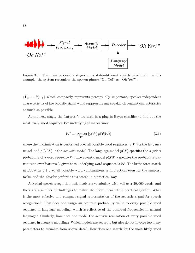
88
ProcessingSignal
ModelAcoustic Decoder
ModelLanguage
"Oh No!"
"Oh Yes?"
Figure 3.1: The main processing stages for a state-of-the-art speech recognizer. In thisexample, the system recognizes the spoken phrase “Oh No!” as “Oh Yes?”.
{Y0, . . . , YT−1} which compactly represents perceptually important, speaker-independent
characteristics of the acoustic signal while suppressing any speaker-dependent characteristics
as much as possible.
At the next stage, the features Y are used in a plug-in Bayes classifier to find out the
most likely word sequence W∗ underlying these features:
W∗ ≡ argmaxW
{p(W) p(Y|W)} (3.1)
where the maximization is performed over all possible word sequences, p(W) is the language
model, and p(Y|W) is the acoustic model. The language model p(W) specifies the a priori
probability of a word sequenceW. The acoustic model p(Y|W) specifies the probability dis-
tribution over features Y given that underlying word sequence isW. The brute force search
in Equation 3.1 over all possible word combinations is impractical even for the simplest
tasks, and the decoder performs this search in a practical way.
A typical speech recognition task involves a vocabulary with well over 20, 000 words, and
there are a number of challenges to realize the above ideas into a practical system. What
is the most effective and compact signal representation of the acoustic signal for speech
recognition? How does one assign an accurate probability value to every possible word
sequence in language modeling, which is reflective of the observed frequencies in natural
language? Similarly, how does one model the acoustic realization of every possible word
sequence in acoustic modeling? Which models are accurate but also do not involve too many
parameters to estimate from sparse data? How does one search for the most likely word
89
sequence during recognition? We detail the state-of-the-art solutions to these problems in
the next few sections. The solutions in most cases are surprisingly simple and effective, given
the complexity and scale of natural language and speech. The key idea is to hierarchically
model speech and language in a modular manner based on statistical principles with some
inspiration from human speech perception.
3.1.1 Speech Signal Processing
The goal in speech signal processing is to compactly represent the information in acoustic
signal that is relevant to word recognition but also in a form useful to the acoustic model.
The information lost during feature extraction cannot be recovered, and hence, it is crucial
in that as much as possible of the information relevant to speech recognition is extracted
during signal processing stage. It is also crucial the extracted information is represented
in a form suitable to the acoustic model. In addition, any characteristics related to the
speaker such as gender and vocal tract, the channel such as handset and microphone, and
the environment such as background noise, need to de-emphasized in features so that sta-
tistical learning algorithms and models can easily extract and represent the variability due
to underlying linguistic context. The dominant acoustic modeling paradigm in the current
speech technology is based HMMs, and the popularly-used speech feature extraction meth-
ods are more or less adapted for HMMs. In this section, we will describe two popular but
quite different feature extraction methods: short-term spectral cepstral features [86] and
long-term temporal patterns [148, 144].
Speech acoustic signal is highly nonstationary, and as such, speech signal processing
methods operate locally on the acoustic waveform. The acoustic waveform is usually parti-
tioned into a sequence of overlapping blocks, called frames, and from each block a 10−20 di-
mensional feature vector is derived. Independent of the particular signal processing method,
a few simple pre-processing operations on the acoustic waveform (such as the subtraction
of DC mean to remove the DC offset introduced in the analog-to-digital conversion and the
pre-emphasis by a high-pass filter to compensate for the attenuation caused by the radiation
from lips) are applied [86, 275]. In addition, the original features from the front-end signal
90
processing unit are subject to a few simple post-processing methods to better match them
HMM-based acoustic models and suppress speaker-dependent variations. In the coming
sections, we will first review the cepstral and TRAPS feature extraction methods and then
describe the post-processing methods that we will use in our experiments.
Cepstral Speech Signal Processing
The most popular feature extraction method in speech recognition is based on the cepstrum,
derived from a smoothed estimate of short-time spectrum. Extraction of cepstral features
from an acoustic waveform typically involves following operations on the acoustic waveform.
First, the acoustic waveform is partitioned into overlapping blocks of duration 25 msec
and spacing 10 msec. Each block of speech is tapered with a Hamming window to reduce
boundary effects, and the Fourier spectrum of windowed signal is taken [220]. The frequency
spectrum is logarithmically divided into 20 frequency bins according to a nonlinear frequency
scale, called mel-scale, which is linear up to 1, 000Hz and logarithmic afterwards. The mel
scale is found to be more effective experimentally than the linear scale for speech recognition,
and it mimics the human auditory system which is more sensitive to the lower part of
the spectrum. The spectral estimate for each frequency bin is then obtained by taking
a weighted average of spectral coefficients within each bin with respect to a triangular
window. After the logarithmic compression of spectral estimates in each bin, discrete cosine
transform (DCT) is applied to the 20-dimensional vector of these spectral estimates in each
block. Usually only the first 12 DCT coefficients are kept (due to reasons explained below).
These coefficients are the so-called mel-scale cepstral coefficients (MFCCs), and they are
used as features in combination with the logarithm of energy in acoustic models. The
various signal processing operations in the derivation of MFCCs are partially motivated
from the source-filter model of speech production, that they couple well with HMM with
Gaussian output distribution acoustic models, and that they perform well experimentally,
which are detailed below.
First, speech is produced by the air released from lungs traveling through vocal tract.
According to the source-filter model, speech production can be modeled as a linear time-

91
invariant system in which the excitation signal e(t) generated at the glottis is filtered by
the vocal tract filter h(t), yielding the acoustic signal s(t) [86]:
s(t) = e(t) ∗ h(t)
where ∗ denotes convolution. The shape of the vocal tract h(t) essentially encodes what
is spoken, and it needs to be separated from the excitation signal e(t), which does not
carry much speech related information, if any. However, it is difficult to separate the vocal
tract information h(t) from the excitation signal e(t) due to the multiplicative form they
appear in the frequency domain. The effect of convolution appears as multiplication in the
frequency domain . However, after logarithmic compression of the spectrum of acoustic
signal, source and channel log-spectra appear additively instead of multiplicatively, which is
easier to separate [211]. In addition, the excitation signal appears as fast changing ripples
in the log-spectrum, whereas the vocal tract appears as the slowly changing carrier. Hence,
the lower-ordered coefficients in the DCT of the log-spectrum are mostly related to the
vocal tract shape, and these are the coefficients that are kept in the cepstral processing.
On the other hand, higher-order DCT coefficients are related to the glottal pulse of the
speaker’s excitation signal and not very useful for speech recognition but useful for speaker
recognition (cf. Section 3.2). Second, logarithmic compression of the spectrum also has a
Gaussianization effect on the resulting feature vectors, which are then better-matched to the
Gaussian output distributions in acoustic models. Similarly, the DCT has a de-correlating
affect and allows the use of diagonal-covariance Gaussian distributions instead of more
costly full-covariance Gaussian distributions in acoustic modeling. In addition, the DCT
compresses the information in the spectral coefficients into a small number of coefficients,
reducing the size of the feature vector for subsequent statistical analysis.
We note that there are alternative ways of deriving cepstral coefficients, most notably
based on an auto-regressive model (also known as linear prediction) of vocal tract in per-
ceptual linear prediction (PLP) cepstrum [143]. In addition, the general shape and length
of the vocal tract of different speakers nonlinearly warp the frequency spectrum of the same
phone uttered by different speakers, and vocal tract length normalization is usually applied
in cepstral processing to map frequency characteristics of different speakers to a normalized
92
representation [261].
TempoRAl PatternS (TRAPS)
The cepstral features are based on a short-time spectral representation of speech around
25 msec windows. The use of such a short-time analysis window in speech recognition has
roots in speech coding where the goal is to compress speech as much as possible with-
out degrading its intelligibility. It has been found in speech coding that such short-term
representations preserving perceptually relevant spectral properties of the speech signal
through linear prediction or subband coding lead to reasonable quality compressed speech
signals [251]. Consequently, speech recognition research has largely adopted the short-time
spectrum as the fundamental representation of the acoustic signal. However, the goal in
speech recognition is not to reconstruct the acoustic signal but to recognize the linguistic
message encoded in the acoustic signal, and there are a number of reasons for why a purely
short-time spectral representation may not be optimal for speech recognition.
First, the goal in speech recognition at the lowest level is to recognize basic sound units
which comprise words. The shortest such linguistically meaningful unit is phone. A phone
can last anytime between 10 msec and 200 msec, and on average there are about 10–15
phones per second. Given the typical duration of a phone, it is clear that a 25 msec window
does not provide all the information necessary to determine the phonetic identity of a given
segment of speech. Second, there are suprasegmental effects such as coarticulation and
lexical stress that affect the acoustic realization of sounds and usually span more than a
single phone. Such long-term effects have also been demonstrated in data-driven corpus
studies [33, 271], where it was shown that there is a significant spreading of linguistic
information across speech frames. Such long-term information and contextual effects are
not explicitly represented in the current HMM-based acoustic models, because they focus on
short-term variability (cepstral features) and context (phones). In addition, the standard
HMM-based acoustic models do not explicitly represent long-term dependence. The use
of such long-term information could aid recognition of underlying sound classes. Third,
there is also psycho-linguistic evidence that humans use information from long-term scales.
93
For example, the preservation of 2–8 Hz modulation spectrum corresponding to 125 to 500
millisecond time scale is critical for speech intelligibility, and human perceptual buffer seems
to hold information from up to 250 millisecond segments of speech [269]. Fourth, using the
spectrum as the fundamental representation of acoustic information is rather fragile against
time- or band-limited noise. Fifth, the short-time spectrum and in turn cepstrum are
partially motivated from our a priori knowledge about the speech production (i.e. source-
filter model, cf. Section 3.1.1) and human auditory system. As such, it is not optimized
and in particular not data driven. As evidenced by the success of data-driven learning
methods in acoustic and language modeling as opposed to knowledge-based methods, there
is potential in learning optimal feature representation a posteriori from data, for improved
speech recognition performance.
TRAPS processing is a relatively new method for data-driven feature extraction from
speech using very long time windows. The basic idea behind TRAPS is to optimize the
feature extraction for recognition by training a first-stage classifier to predict a set of basic
sound classes using long-term information and then use the outputs of this first-stage classi-
fier as features in a conventional speech recognition system. Similar to the cepstral feature
extraction, TRAPS are extracted on a frame by frame basis, for example, once every 10
msec, but the frame window size is much longer, typically about 500 msec, centered around
the time at which features are extracted. A typical processing of TRAPS features for each
speech frame is as follows [148, 144, 146]. First, energy trajectories for about 15 critical fre-
quency bands are calculated for the given window size [5]. Then, each critical-band energy
trajectory is input to a separate neural-network classifier predicting phones or some other
processing unit such as syllable structure and stress (cf. Chapter 4). Each critical-band
neural-network outputs a vector of a posteriori probabilities corresponding to the predicted
units. All such outputs from each critical-band neural network are then input to a merger
neural network which again predicts phones or some other units and outputs a posteriori
class probabilities for them. These a posteriori class probabilities after taking logarithms
and applying principle component analysis are the TRAPS features. The dimensionality
of TRAPS features depends on the cardinality of the neural-network targets, for example
they are of the dimension 40− 50 if the neural networks are trained to predict phones. The
94
critical band neural networks as well as the merger neural network are trained from data
using the frame-level class labels, which are usually not available, and instead the Viterbi
assignments from an existing speech recognizer are used as if they were the true labels.
In the literature, a number of variations on the above processing steps has been pro-
posed [60, 61, 12]. We will also use hidden activation TRAPS (HAT) [60, 61] variation in
some of our experiments. The HAT processing differs from TRAPS processing mainly in that
it eliminates first-stage critical-band neural networks and uses a single-stage neural-network
architecture to predict phones or some other units from critical-band energies. See [60, 61]
for more information about HATs. Overall, TRAPS and variations such as HATs automat-
ically discover discriminative patterns in long-time windows of speech. TRAPS are largely
complementary to short-time cepstral features, and as such, they are typically used in combi-
nation with them. For example, in a recent NIST Hub5 speech recognition evaluation, they
are found to significantly boost the performance of a state-of-the speech recognizer [279].
Post-processing Methods
Independent of feature kind, it has been found in the speech recognition literature that
simple post-processing techniques can significantly improve speech recognition accuracy. In
this section, we will describe two such techniques, dynamic features (the so-called delta and
double-delta features), and speaker and channel normalization by mean subtraction and vari-
ance normalization. The basic idea behind these and other post-processing techniques on
features is to better match the original features to the HMMs with Gaussian output distri-
bution statistical models and normalize features across different speakers and/or handsets.
In HMM-based speech recognition systems, a frame-based sequence of features {Y0,. . . ,
YT−1} is usually augmented with their first- and second-order differences, delta and double-
delta features, respectively. The delta feature Yt for the t-th frame is obtained from the
static features {Yt} according to a linear regression over a window of 2K+1 frames centered
around the current frame:
Yt ≡∑K
k=−K k Yt+k∑Kk=−K k2
.
The double-delta features are similarly obtained but from the delta features. Even though
95
the use of such dynamic features is standard, a clear understanding of why they are useful
for speech recognition is missing. The delta and double-delta features are deterministically
related to the original sequence of features, and as such, all the information that they
contain is already in the original sequence of features. There exist a number of hypotheses
for why they are useful, but their usefulness seems to be mainly due to the fact that the
modeling assumptions made in the current HMM-based acoustic models are not realistic for
a highly correlated sequence of frame-based features. According to one hypothesis [73], the
rate of change information provided by the dynamic features partially alleviates the HMM
assumption that observations are independent of each other given states, which do not hold
for frame-based features. According to another one [39], by appending the dynamic features
to original features and not characterizing the deterministic relationship between the static
and dynamic features (i.e. making an incorrect modeling assumption), the appended features
can only provide more information about the underlying states and hence words.
In many speech recognition systems, it is also standard to normalize a given sequence
features by subtracting the mean and dividing by the standard derivation calculated over
all frames coming from a particular speaker and/or handset [11, 125]:
Xit ≡
Y it − µi
σi(3.2)
where Y it denotes the i-th component of feature vector time t; µi and σi denote the cor-
responding sample mean and variance, respectively, of features coming from a particular
speaker and/or handset; and Xit is the transformed feature component. The motivations for
the normalization in Equation 3.2 are two fold. First, for the cepstral features, the convolu-
tive effect of transmission lines appears as an additive offset, and such convolutive noise can
be partially removed by subtracting the mean cepstral vector from all vectors coming from
the same transmission line [125]. In addition, variance normalization compensates for addi-
tive noise [63]. Second, applying the transformation in Equation 3.2 across features coming
from a particular speaker and/or a handset is a simple form of speaker adaptive training
where various sources of variability such as speaker or handsets are modeled as linear trans-
formations on a purely linguistic-message-dependent acoustic feature representation (Xit in
Equation 3.2) [8, 173].
96
In our experiments, we will employ dynamic features and speaker-level mean subtraction
and variance normalization. We note that other feature transformation methods such as
heteroscedatic linear discriminant analysis [172] are also commonly used in state-of-the-art
recognition systems but not used in this thesis.
3.1.2 Language Modeling
The language model, p(W) in Equation 3.1, provides the a priori probability for any given
sequence of words, W ≡ {W0, . . . ,WN−1} for Wk ∈ W, where Wi denotes the i-th word
in a sequence of N words, and W is the vocabulary. Given that there are exponentially
many word combinations even for the smallest vocabularies, it is impossible to explicitly
estimate the probability of each and every word sequence from data. A simple yet effective
mechanism for assigning probabilities to word sequences is n-gram language modeling, which
characterizes the language as an (n− 1)-th order time-homogeneous Markov chain [159]. A
n-gram language model does not explicitly encode any syntactic and semantic constraints in
the language, but they indirectly encode such constraints and others to the extent that the
unallowed combinations do not appear in the training data. The n-gram language models
are particularly effective for languages such as English where word ordering is important
and the strongest contextual effects come from neighboring words. Typical values for n are
two and three corresponding to the bigram and trigram, respectively, language models.
A bigram language model characterizes the probability of a word sequence {W0, . . . ,
WN−1} as
p(W0 = w0, . . . ,WN−1 = wN − 1) ≡ p(w0)N−1∏k=1
p(wk|wk−1).
The unigram probabilities p(w0) and the bigram probabilities p(wk|wk−1) are estimated
from the word and word-pair, respectively, frequencies in a large training corpus, which are
the maximum-likelihood estimates. However, even for a medium vocabulary consisting of
5, 000 words, there are 2.5 million unique bigrams; most of them will be not be observed
in training data; and hence, they will be assigned zero probability. Such zero probability
estimates are not desirable, since hypotheses containing corresponding pairs of words will be
97
directly eliminated during decoding in speech recognition. A solution to this problem is back-
off which involves replacing unobserved or very sparse bigram pair (wk−1, wk) probabilities
by the scaled unigram probabilities [64]:
p(wk|wk−1) ≡
N(wk−1,wk)−D
N(i) if N(wk−1, wk) > t
b(wk−1)p(wk) otherwise(3.3)
where N(wk−1, wk) is the number of times that the word wk follows the word wk in the
training corpus; N(wk) is the number of times that the word wk appears; t is the bigram
count threshold; D is a pre-determined discount constant; and b(wk−1) is the back-off weight
for the word wk−1 and set so that p(wk|wk−1) in Equation 3.3 is a valid probability distri-
bution. The trigram language models are defined similarly to the bigram language models
by backing-off to the bigram probabilities for the sparse trigrams in the training data. The
trigram language models are the most popular language models in the state-of-the-art large
vocabulary speech recognizers.
One of the measures for the difficulty of a speech recognition task is defined through
language models. We expect a recognition task to be more difficult if there are more possible
words that can follow a word at a given time, and the language model does not clearly
predict one word against the others based on the history. Perplexity is a quantification of
this concept and defined as 2H(p) where H(p) is the entropy rate calculated with respect to
the language model p using a large corpus {w0, . . . , wN−1} [18]:
H(p) ≡ − 1N
N∑k=1
log p(wk|wk−1, . . . , w1).
The perplexity strongly depends on the task domain. For example, the perplexity of conver-
sational English in the Switchboard corpus is around 110 and 90 with respect to bigram and
trigram, respectively, language models and a 23, 000 word vocabulary [73]. On the other
hand, the perplexity in a more constrained air travel information service domain is around
15 with a bigram language model and a 2, 000 word vocabulary [280].
3.1.3 Acoustic Modeling
The acoustic model, p(Y|W) in Equation 3.1, in a speech recognition system provides a
probability distribution over the acoustic feature sequence Y given that the word sequence
98
W is uttered. Again, it is not possible to estimate a probability distribution for every
possible word sequence, and we need a practical way of modeling acoustic observation
distributions for any sequence of words. The solution to this complex modeling problem
in large-vocabulary speech recognition comes from hierarchical modeling where models for
word sequences are composed from models for a small set of basic sound units from which
words are comprised of. Typically phones are used as the basic sound units, but other
subword units such as syllables [114, 269] and automatically derived subword units [17] have
also been proposed for this purpose. In our review of the state-of-the-art acoustic modeling
below, we will use phones as the basic modeling blocks, but we will argue in Chapter 4
that both phones and syllable structure and lexical stress should be characterized for better
characterizing acoustic variability associated with conversational speech. In English, there
are about 50 phones.
Hierarchical modeling of speech in acoustic modeling is done at two levels. Utterances
are first decomposed into words, and each word in the sequence is then decomposed into its
phones using a pronunciation dictionary. The resulting composition is a network of phones
corresponding to that utterance. If a word has multiple pronunciations, then multiple phone
paths, one for each pronunciation, are used. Now, if we can accurately model each phone
occurring in the pronunciation dictionary, then we have a practical method of composing
acoustic models for every word sequence. Given an acoustic model for each phone, the acous-
tic model for an utterance is obtained by inserting the model for each phone in the network
of phones corresponding to that utterance. The acoustic score of a sequence of acoustic
features for that utterance can then be efficiently calculated by a dynamic programming
algorithm which is similar to the forward pass in the forward-backward algorithm of HMMs.
An HMM is the most commonly used model for characterizing phones. Each phone is
typically represented as a three-state left-to-right HMM. The begin, middle and end states
in these phonetic HMMs characterize sub-phonetic variability associated with different parts
of the phone. The output distributions of the phonetic HMM characterize acoustic feature
vectors, and considering their large dimensionality (about 39), it is important that they
are accurately and efficiently characterized. The mixture of Gaussian models combine the
advantages of parametric and non-parametric modeling, and they are commonly used to
99
represent output distributions in phonetic HMMs. Typically, between 12 and 32 mixture
components per state are used, depending on the amount of training data.
Phonetic HMMs that we have described in the previous paragraph are context-independent,
because each phone is considered as a monophone without taking its context into account.
However, the contextual effects such as coarticulation can have a large impact on the acous-
tic realization of phones. To represent such contextual effects, context-dependent phones
are used, and the versions of the same phone with different left and right contexts are
distinguished. Triphones consider each phone along with its immediate left and right neigh-
bors. For example, the triphone sequence for the utterance “Oh no!” with a phonetic
pronunciation “oh n ow” is given by
sil-oh+n oh-n+ow n-ow+sil
where the notation x-y+z refers to the phone y preceded by the phone x and followed by
the phone z. The triphone expansion in the above example go over word boundaries, and
such triphones are called cross-word triphones. Cross-word triphones considerably increase
computational costs of decoding, and a simpler alternative is �word-internal triphones where
contexts outside of word boundaries are ignored.
Triphones and high-order context-dependent units are more accurate than monophones,
but they also come with estimation problems due to data sparsity. There are about 60, 000
unique triphones in English. Even in a fairly large speech corpus such as Switchboard
consisting of about 250 hours of data, many triphones do not occur at all or occur very few
times [275]. A solution to this problem comes from parameter tying where the parameters of
the triphones which are acoustically similar to each other are tied together. In the so-called
state-tying approach, the states of all triphones of a phone at a particular state position
are partitioned into clusters using phonetic decision trees [274]. There are separate decision
trees for each phone and state position, and at each node of a tree there is a linguistically
motivated question such as “is the phone on the right-hand side a vowel?”, or “is the
phone on the left-hand side as syllabic?”. (An advantage of using phonetically motivated
questions is that one can synthesize models for every triphone, regardless of whether it
occurs in training data or not [275].) The leaves of these phonetic decision trees are the
100
state clusters, triphone states which have been tied together. State-tying decision trees
are usually induced from data according to the following greedy procedure. First, all data
corresponding to a particular phone and state position are collected at the root of the tree.
Then, iteratively, for each leaf node and question in a pool of pre-determined questions, the
likelihood increase due to the resulting split is calculated. The leaf node giving the highest
likelihood is partitioned into two leaf nodes, and the corresponding question is recorded.
The tree is grown until either the increase in likelihood is below some threshold, or the data
at the new leaf nodes are too sparse for accurate estimation of a state-output distribution,
again typically determined by a heuristic threshold.
3.1.4 Decoding
Decoding in speech recognition is the process of finding the most likely word sequence W∗
corresponding to an acoustic feature sequence Y (cf. Equation 3.1). In some applications
such as a travel reservation system, what speakers say is restricted in the grammar, and the
search is performed only over allowed word sequences. However, in many cases, in particular
in conversational speech, there is not any restriction in what speakers say, and the search
needs to be performed over all possible word sequences.
During the search, the language model, lexicon, and sub-word units are first compiled
into a composite model with hidden variables at word, phone and state levels. The most
likely word sequence is then obtained by finding the Viterbi assignment to the hidden vari-
ables of the composite model using dynamic programming.1 The computational cost of the
search is mainly determined by the size of the state space of the composite model, which
depends on, among other parameters, vocabulary size, order of the language model, number
of tied states, and word-internal vs. cross-word triphone modeling. For example, decoding
with a bigram language model is much less costly than decoding with a trigram language
model; and decoding with cross-word triphones practically amounts to the squaring vocab-
1Notice that this dynamic programming search finds the joint Viterbi sequence for both words and statesand not the most likely word sequence. As such, multiple pronunciations of the same word are scoredseparately instead of summing over their scores. Nevertheless, the most likely joint state sequence andpronunciation usually accounts for most of the probability of that word, and the joint Viterbi approach isjustifiable.
101
ulary size, and as such, they are more costly than decoding with word-internal triphones,
or monophones.
The search for the most likely word sequence in the composite model is performed
using dynamic programming, which is essentially the same as the Viterbi algorithm that
we described in Section 2.6.2 for HMMs. A typical utterance involves hundreds of frames,
and there are thousands of words even in a medium-sized recognition task. Hence, the
state space is very large, and the exhaustive search even with the most efficient dynamic
programming techniques with special data structures is near to impossible. To make the
search feasible, modern speech recognizers employ a number of specialized techniques such
as tree-structured lexicons, caching of Gaussian scores from the HMM output distributions
(Gaussian evaluations take most of the computation decoding decoding), and pruning of
unlikely partial hypotheses. For a through introduction to large vocabulary search, see [205].
An alternative to the first-pass decoding, where the most likely word sequence is search
from the scratch, is multiple-pass decoding, where simpler acoustic or language models are
first used to generate a set of alternative hypotheses which are then re-scored using more
complex models. The alternative hypotheses could be represented as a word lattice in which
every valid path from the entry to exit of the lattice is a recognition hypothesis. A simpler
representation is an n-best list, which is a list of n distinct sequences of words for each
utterance.
A practical issue in first-pass decoding, or n-best rescoring is that dynamic ranges of
acoustic model scores tend to be much larger than those of language model scores. If the
language modeling scores were used as they are, they would have little, or no effect on the
final recognition output. To circumvent this problem, it is customary to scale the language
modeling probabilities by a factor in the log-domain (typically about 10 for the logarithm
base 10). In addition, an insertion penalty per recognized word is applied to control for
deletion and insertion errors. As we will do, the language model scaling factors and insertion
penalties are adjusted on an independent testing set.
102
3.1.5 Evaluation Metric
Performance of a speech recognition system on a collection of test utterances is evaluated
with respect to the word error rate metric, which is defined as
E ≡ S + I +D
N100
where E denotes the word error rate, N is the number of words in the reference tran-
scriptions, and S, I, and D are the number of word substitutions, insertions and deletions,
respectively, in the hypothesis transcriptions when compared to the reference transcriptions.
The comparison is done by an optimal string match between the reference and hypothesis
transcriptions to minimize the total cost of alignment. For example, in the NIST scoring
tool sclite which we will use, each substitution, insertion, and deletion error carries a cost
of 4, 3, and 3, respectively [275, 3]. It is standard in speech recognition evaluations to not
to count acoustically indistinguishable alternatives (such as worldview vs. world view) as
errors by filtering reference and recognition transcriptions for alternate spellings and word
contractions.
3.1.6 Experimental Paradigms
Tasks
We will perform speech recognition experiments in two English continuous speech recogni-
tion tasks, which we will refer to as short Hub5 (sh5) and new short Hub5 (nsh5).2 The
tasks sh5 and nsh5 mimic a large vocabulary speech recognition task (which involves hun-
dred hours of training data and requires huge computational resources for training and
decoding) on a smaller scale to allow fast experimental turn-around. It has been shown
that they fulfill this goal to a large extent and new techniques developed on these tasks
transfer to the much-larger recognition tasks [199, 62].
Both sh5 and nsh5 tasks extract their training and testing data from standard speech
corpora: Switchboard, Callhome, Macrophone, and Numbers ’95. Switchboard consists
2The tasks sh5 and nsh5 are originally defined and used by a multi-university research team exploringnovel speech recognition methods for the DARPA EARS program [2]. Their training sets have roots in adata set originally defined at SRI for internal system development.

103
of short spontaneous telephone conversations between two strangers on pre-defined topics
such as weather and care for the elderly [124]. Callhome is similar to Switchboard except
that conversations take place between friends without any topic restriction [180]. As a
result, the speech in Callhome is more causal and more difficult to recognize. Macrophone
is designed to provide telephone speech for voice-interactive telephone services, such as
shopping [28]. It is not conversational but spoken and consists of utterances about times,
locations, and monetary sums. Numbers ’95 is similar to Macrophone and consists of
utterances of telephone numbers, zipcodes, and other miscellaneous items involving number
sequences [72].
Short Hub5 is a small vocabulary spontaneous speech recognition task, that of recogniz-
ing number sequences. Even though the testing is done on number sequences, the training
data consists of conversational speech utterances and not only numbers. The training set
of sh5 is gender balanced and consists of 18.7 hours of speech, of which 4.4 hours come
from Callhome, 2.7 hours from part of Switchboard which is hand-transcribed at SRI, 2.0
hours from the Credit-card portion of Switchboard, and 9.6 hours from Macrophone. The
testing set of sh5 consists of 1.8 hours of speech from Numbers ’95, of which we allocated
0.6 hours for cross-validation in system development, and a separate 1.2 hours for testing.
We will report recognition results only on the latter portion. We note that the testing set of
sh5 is mismatched to its training set in both speaking style and vocabulary coverage. This
was an intentional choice to avoid tuning to a particular task in system development and
to facilitate transfer of new techniques to the large vocabulary tasks. The acoustic models
trained for this task have broad phonetic coverage similar to the acoustic models in large
vocabulary speech recognition. At the same time, the decoding vocabulary for Numbers
’95 only involves about 30 words which allows for first-pass decoding with complex acous-
tic models without resorting to multiple-pass search strategies which would be otherwise
necessary. Our focus in this work is acoustic modeling, and we will use a fixed back-off
bigram language model in all experiments in sh5. This language model is trained on the
transcriptions of the part of the Numbers ’95 corpus that we did not use in testing.
New Short Hub5 is a medium vocabulary conversational speech recognition task, which
is a scaled-down version of the 2001 NIST Hub-5 recognition task used for evaluating large

104
vocabulary speech recognizers, in terms of both the amount of training data and the vocab-
ulary coverage during testing. The training data of nsh5 consists of 68.8 hours of speech,
of which 61.6 hours come from Switchboard, 3.3 hours from Callhome, and 3.9 hours from
Cellular portion of Switchboard. There is slightly more training data (52%) for female
speakers, because this is also the case for the full Hub-5 training collection. Unlike sh5,
nsh5 does not contain any data from Macrophone (read speech), and all of the training
data is conversational and similar to the testing data. The testing data of nsh5 is about
a .9 hour subset of the 2001 NIST Hub-5 evaluation data, selected as follows. Given the
500 most frequent words in Switchboard, we choose utterances from the Hub-5 2001 eval-
uation data with an utterance-level out-of-vocabulary (OOV) rate3 that is less than 7.5%
with respect to these 500 words. About half of utterances in the 2001 Hub-5 evaluation
set met this requirement. We partitioned this 0.9 hour subset into separate cross-validation
(22%) and testing (78%) sets, which do not overlap in their speakers. All recognition results
on this task are reported on the later testing set. During recognition, we used a lexicon
consisting of the 2, 500 most frequent words, resulting in an overall OOV rate of 1%, which
is similar to the OOV rates in large-vocabulary speech recognition tasks. The language
model in our nsh5 experiments is fixed to a back-off bigram LM which has been trained on
a number of text resources, Switchboard, Callhome, Switchboard Cellular, and Broadcast
News transcriptions. Other than the vocabulary coverage, it is similar to the one used at
SRI for the 2001 Hub-5 evaluations.
By testing on the utterances which mostly include the 500 most frequent words in the
nsh5 task, it is expected that new techniques proven to be useful on this task are also likely
to be useful on full-vocabulary CTS tasks. The choice of testing set in nsh5 also justifies
the use of a smaller training set than that would be needed for full-vocabulary tasks, as
there are many examples of these 500 words in the training data [199]. In terms of amount
of training data, vocabulary size, and speaking style, nsh5 is much more challenging than
sh5 and closer to the full-vocabulary tasks. Yet, it does not require the large computational
resources and infrastructure necessary for testing on full-vocabulary tasks.
3The OOV rate of an utterance is defined as the percentage of word tokens that are not covered by thevocabulary.

105
Baseline Recognition System
In this section, we will describe training and testing procedures for a triphone tied-state
HMM continuous speech recognition system, which closely follow the recipe given in [275].
Similar systems that are trained on either different kinds of features or acoustic modeling
units will serve as seed models in our speech recognition experiments in the later chapters.
Such a system involves millions of parameters and is built in many inter-related stages from
acoustic feature vectors, training transcriptions, and a pronunciation dictionary. During
training, the complexity (such as the number of mixture components at the HMM output
distributions) is introduced in a controlled manner, and a simpler system at a particular
stage is used to initialize the more complex system at the next stage. Briefly, first a set
of monophone models are trained. These monophone models are then used to determine
tied-state clusters and initialize their distributions, which are further trained according to
a mixture splitting schedule until the desired number of Gaussian mixture components per
tied-state is achieved. The detailed description of these steps is given below.
1. Initialize monophone HMMs with single component diagonal-covariance Gaussian out-
put distributions by globally setting their means and variances to the sample mean
and variance, respectively. Expand each training utterance into phones using the first
available pronunciation for each word in the dictionary.
2. Apply 5 iterations of embedded EM estimation. Force align training sentences into
phones.
3. Determine triphones occurring in the training data and clone models for them from
monophone models.
4. Apply 2 iterations of embedded EM estimation. Obtain the sufficient statistics neces-
sary for tied-state clusterings. Induce the state-tying decision trees and initialize their
parameters.
5. Apply 5 iterations of embedded training. Force align training sentences into phones.

106
Split each Gaussian mixture component at the tied-state output distributions into
two.4
6. Repeat Step 5 until the desired number of mixtures is achieved.
Throughout training, acoustic models are estimated from phone sequences by embed-
ded training, as neither the segmentation of training utterances into words nor the phone
segmentation of each word into its phones is available. Phone transcriptions are obtained
by either randomly picking a pronunciation in the dictionary (in Step 1), or forced-aligning
word transcriptions into phone sequences using existing acoustic models at the later stages.
Most words in dictionary have a single pronunciation. Thus, the main effect of performing
forced alignments throughout the training procedure is to refine the presence or absence
of silences or pauses between words. Also, the training procedures for word-internal and
cross-word triphone models are exactly the same except in the state clustering stage (Steps 3
and 4) with obvious modifications.
We will use both first-pass decoding and n-best rescoring for testing. The sh5 task
involves recognition of number sequences with a vocabulary size of about 30 and allows for
first-pass decoding even with complex acoustic models. Thus, all recognition experiments
on this task are performed using first-pass decoding. However, the recognition lexicon in the
nsh5 task is relatively large, 2, 500, and we will use an n-best (n = 500) rescoring paradigm
in experiments involving relatively complex acoustic models.
Software
We will use the Hidden Markov Toolkit (HTK) [275] and the Graphical Models Toolkit
(GMTK) [41] to build and test speech recognition systems. HTK is a set of modules for
training and testing HMM-based speech recognition systems, and it is extensively used in
the speech recognition literature. We will make frequent use of HTK to train triphone
HMM systems according to the procedure given in the previous section. HTK also includes
4HTK splits of a Gaussian component in a mixture by copying that component, dividing weights of bothcopies of that component by two, and perturbing their means by plus and minus 0.2 standard deviations.GMTK uses a similar splitting scheme but with random perturbations.
107
a fairly efficient medium-vocabulary decoder (HVite) that accepts bigram language models.
Whenever we use HTK, we will employ first-pass decoding in our experiments in both sh5
and nsh5. HTK will also be used to generate the n-best lists and tied-state clusters for our
experiments in GMTK.
GMTK is a general purpose toolkit for speech, language, and time-series modeling us-
ing graphical models. It has been successfully used in a number of speech recognition
tasks ranging from small- [281] to medium-vocabulary [80]. For our purposes, GMTK al-
lows for straightforward implementation of a wide range of acoustic models which include
HMMs and the models beyond HMMs, and such, we will extensively use GMTK in our
experiments exploring more sophisticated acoustic models. During the course of this thesis,
GMTK has been continuously developed. In our experiments in Chapter 5, we used the
first implementation of GMTK as described in [41], whereas those in Chapter 4 used the
later pre-alpha second version with a new inference engine [40]. We will use the GMTK
decoder gmtkViterbi in our experiments in sh5 for first-pass decoding, and the junction
tree inference engine gmtkJT in our experiments in nsh5 with n-best rescoring.
3.2 Speaker Recognition
Speaker recognition is the process of recognizing speakers from their voices. As a biomet-
ric, speaker recognition provides an economical authentication method in human-machine
interactions such as telephone banking and voice mail [113]. Speaker recognition also has
obvious forensics and security applications [58]. It is also a crucial module in extracting
meta information from the speech signal, such as automatic annotation of meetings with
speaker turns and identities in addition to what was spoken. Speaker recognition tasks can
be divided in speaker identification and speaker verification. Speaker identification is con-
cerned with determining which speaker in a group of known speakers has spoken, whereas
speaker verification is concerned with verifying the claimed identity of a known speaker, also
called a target speaker. Speaker verification only involves a binary decision, but it is not
necessarily easier than speaker identification due to the fact that an open set of impostors
needs to be considered in decision making. Speaker recognition systems are also distin-

108
ProcessingSignal
SpeakerModel
BackgroundModel
> τΛAccept if
> τΛReject if
+_
Figure 3.2: The main processing stages for a state-of-the-art speaker verification system,adapted from [227].
guished based on whether they are text-dependent or text-independent. In text-dependent
speaker recognition, speakers are required to say a known phrase, whereas there is no such
restriction in text-independent speaker recognition. Text-independent recognition is more
difficult because of the additional text-dependent variability that needs to be separated from
the speaker-dependent variability. In this thesis, we will be interested in text-independent
speaker verification.
Humans rely on multiple levels of information to identify speakers from their voices.
They use low-level acoustic cues due to vocal tract shape and larynx as well as high-level
cues such as speaking style, word usage, pronunciation, and prosody. On the other hand,
most automatic speech recognition systems primarily exploit low-level acoustic information
especially for recognition with at most couple of minutes of speech, but the use of high-
level information such as word usage is an active research area [226]. Nevertheless, the
performance of the current speech recognition systems are quite impressive and under some
conditions comparable to human performance, an exception in human language technolo-
gies [228]. The most common approach to text-independent speaker verification is to apply
a likelihood-ratio test to accept or reject the claimed identity [230]. The basic components
of such a verification system appears in Figure 3.2.
Given an acoustic signal A, first a sequence of features Y ≡ {Y0, . . . , YT−1} is extracted.
These features are then used to test the hypothesis that Y is from the hypothesized speaker
109
S against the null hypothesis that it is not:
H0 : Y is from the hypothesized speaker S
H1 : Y is not from the hypothesized speaker S.
It is well-known in the statistical decision theory that the optimal test at a given level of
missed detections or false alarms is the likelihood-ratio test
p(Y|H0)p(Y|H1)
H0
≷ τ
H1
(3.4)
where the acceptance threshold τ determines the level of missed detections (or false alarms).
The likelihoods p(Y|H0) and p(Y|H1) in Equation 3.4 are calculated using the models for
the speaker S and the impostors for that speaker. The model for the impostors is commonly
referred to as the background model. Speakers and impostors are usually characterized by
separate Gaussian mixture models (GMMs) [230]. In the next few sections we will describe
these components of the GMM-based speaker recognition systems in more detail.
3.2.1 Signal Processing
The goal in signal processing for speaker recognition is to extract features that emphasize
speaker-dependent characteristics. Somewhat surprisingly, MFCCs are also a popular choice
due to their experimental success, and they are extracted exactly the same way that they are
extracted for speech recognition (cf. Section 3.1.1), except that more cepstral coefficients are
used in speaker recognition than in speech recognition (typically, 16 vs. 12). The main reason
for this difference is that higher-order cepstral coefficients are related to the glottal pulse of
the speaker (as we have argued in Section 3.1.1). Similar to the feature post-processing in
speech recognition, delta features are also used, and cepstral mean subtraction is employed
to combat convolutive channel noise.
3.2.2 Speaker and Background Modeling
The speaker and background models in most speaker recognition systems are represented by
mixture of Gaussian distributions. As such, any time and order information in the acoustic
110
signal, which is mostly related to the word content, is ignored. For text-independent speaker
recognition, this ignorance assumption has the desired effect of not characterizing variability
due to differing word contents during speaker enrollment and later use, and it works well
in practice. There are a number of approaches to constructing speaker and background
models. The simplest approach is to train a separate model for each speaker using his or her
own data and a common background model for all speakers, called a universal background
model (UBM), using data from a large set of impostor speakers representing the general
population. We will simply refer to this modeling approach as the GMM-UBM speaker
recognition modeling. In a GMM-UBM speaker recognition system, the GMM λS for the
speaker S is given by
pλS(Y) ≡
T−1∏t=0
M∑m=1
αmN (yt;µm,Σm) (3.5)
where M is the number of mixture components, and αm, µm, and Σm are the mixture
weight, mean vector, and covariance matrix, respectively, associated with the m-th mixture
in that model. The universal background model λ is similar to the speaker model λS in
form. The parameters of the speaker and background models are usually estimated using
the EM algorithm from their own training data. During testing, the speaker and background
models, λS and λ, respectively, are then used to evaluate the likelihoods for the hypotheses
H0 and H1, respectively, in the likelihood-ratio test of Equation 3.4.
In some applications, it could be desirable to model the background speakers for each
speaker separately, as, for example, impostors might try to claim for speakers that sound
similar to them or are of the same gender. In such cases, speaker-specific background
models are built using data from a specific group of impostors. However, most state-of-
the-art speaker verification systems employ a variation of the GMM-UBM system described
above [227]. Similar to the GMM-UBM systems, a universal background model is used, but
instead of training each speaker model from scratch using its own data, they are derived by
the maximum a posteriori adaptation of the universal background model to that speaker.
Roughly speaking, the resulting speaker and background models are coupled, which is found
to not only give better performance but also exploited for fast Gaussian calculations and
pruning [202].
111
3.2.3 Decision Making
Given a sequence of features Y, the decision for accepting or rejecting the claimed identity
S is made by according to the likelihood-ratio test in Equation 3.4, or equivalently, by
comparing the log-likelihood ratio statistics,
Λ(Y) ≡ log pλS(Y)− log pλ(Y) (3.6)
to some fixed threshold. The score Λ(Y) needs to provide an absolute calibrated measure
across utterances of variable duration and unconstrained word content. The score normal-
ization provided by the background model in Equation 3.6 is useful for this purpose, because
it partially alleviates non-speaker related variations due to the word content, handset, and
emotional state of the speaker. The dynamic range of Λ(Y) in Equation 3.6 depends on
the length of the feature sequence, and as such, it is standard to normalize Λ(Y) by the
utterance length T . In addition to utterance length normalization, a number of other nor-
malization methods such as H-norm [229] and T-norm [15] can be applied to obtain statistics
that are more robust to handset and utterance variations, but such advanced methods will
not employed in our experiments.
3.2.4 Evaluation Metrics
The performance of speaker recognition systems is evaluated by the rate of missed detections
and false acceptances in a testing set consisting of utterances from target speakers and
impostors. The receiver operating characteristics curve is used to display the rate of missed
detection against the rate of false alarms at a number operating points, obtained by varying
the acceptance threshold τ in Equation 3.4. In speaker recognition, the receiver operating
characteristics curve is usually plotted on a special coordinate system such that if the curve
for a binary classification problem involving two equal-variance Gaussian distributions was
plotted, it would appear as a straight line. This curve is called detection error trade-off
curve, and it helps distinguish between different high-performance systems. A number of
points on this curve are of special interest. The equal error rate point is the point at which
the rate of missed detections is equal to the rate of false alarms. Another point of interest
112
is the point at which the detection cost function (DCF) is minimized. The DCF with cost
factors cmiss and cfalse for the missed detections and false alarms, respectively, is given by
DCF ≡ cmiss p(target) pe(miss) + cfalse p(impostor) pe(false) (3.7)
where p(target) and p(miss) are the a priori probabilities for the target and impostor,
respectively, speakers; and pe(miss) and pe(false) are the rates of missed detections and
false alarms, respectively. Depending on the cost factors and the a priori probabilities,
different regions of the receiver operating curve becomes more relevant, e.g. the low false
alarm region, if the false alarms are much more costly than missed detections as in the 1996
NIST speaker verification evaluations, cf. Section 3.2.5.
3.2.5 Experimental Paradigms
Task
We will use the NIST 1996 speaker verification benchmark as our speaker verification
task [1]. The emphasis on this benchmark at the time that it was conceived was the effects
of handset variation and utterance duration on the speaker verification performance. As
such, this benchmark includes a number of training and evaluation conditions, and we will
use the “one-session” training/testing condition in our experiments in Chapter 6.
In the training set of one-session condition, there are 21 male and 19 female target
speakers, and for each speaker, a roughly 2 minute speech segment taken from a single
conversation in the Switchboard corpus is provided. (The training segments are obtained
by concatenating consecutive speaker turns in a conversation, and as such, they do not
correspond to one single contiguous block of speech from one utterance.) The training
segment for each speaker only includes speech from a single handset (more correctly, a
telephone number). Similarly, the data from 43 male and 45 female impostors are provided
for background modeling. In the testing set of one-session condition, there are utterances
of nominal duration 3, 10, and 30 seconds. For each testing duration, there are about 600
trials from target speakers and about 1050 trials from impostor speakers. Of the 600 target
speaker trials for each testing duration, about half come from the same handset used in the
113
corresponding speaker’s training segment, whereas the remaining trials come from a different
test set. The impostor speakers in tests are different from the impostor speakers provided
as part of the training data. There are 204 such male impostors and 172 female impostors
in the testing data sets. The target trials as well as the impostor trials include roughly
equal amounts of data from male and female speakers. In our experiments, we will evaluate
the performance separately for each testing duration and whether or not the target trials in
testing come from the handsets in the training data (matched and mismatched, respectively,
training and testing). The impostor trials in matched and mismatched conditions will use
the same set of impostor trials.
During evaluation, each trial produces N binary speaker verification tests (N being the
number of target speakers), one for each target speaker. The speaker verification system
outputs a score for each target speaker and each trial, where the more positive the score, the
more likely the corresponding target speaker. An utterance coming from a target speaker is
evaluated as an impostor claimant for all other target speakers, whereas utterances coming
from non-target speakers are evaluated as impostor claimants for all target speakers. To
evaluate the performance in a particular condition, the scores from all testing utterances
are pooled together, and a detection error trade-off curve is plotted using empirical missed
detection and false acceptance rates for a range of acceptance thresholds, common to all
speakers. In our experiments, we will report the equal error rate and the minimum detection
cost function in Equation 3.7 with the following cost factors and a priori probabilities for
target speakers and impostors: cmiss = 10, cfalse = 1, p(target) = .01, and p(impostor) = .99,
as used in the 1996 NIST evaluations.
Baseline Verification System
Our baseline speaker verification system is a GMM/UBM system as described in Section 3.2.
For the features, we use 16 MFCCs and their first-order differences over a 4 frame window
as features and apply utterance-level cepstral mean subtraction. For each target speaker,
we train a GMM from that speaker’s training data using the EM algorithm. Similarly,
we train a universal background model for all speakers by fitting a GMM to data from all

114
impostors, male and female. The following procedure is used to separately train speaker
and background models:
1. Initialize the GMM by a single component Gaussian distribution with mean and co-
variance matrix set to the sample mean vector and covariance matrix, respectively.
2. Split the Gaussian component into two. Re-estimate parameters using the EM algo-
rithm for a maximum of 10 iterations, or until the relative increase in the log-likelihood
is below 10−5.
3. Repeat step 2 until the desired number of mixtures are reached.
4. Further train the full mixture model for a maximum of 250 iterations until the relative
increase in the log-likelihood is below 10−5.
The 250 iterations at the last step is a very conservative estimate for the convergence of
the EM algorithm, and the convergence is almost always achieved in fewer than 50 iterations.
We report results with models with varying complexity up to 32 mixture components per
speaker and background model.
Software
We have performed our speaker recognition experiments using the C++ software that we
developed in this thesis.
3.3 Machine Tool-Wear Condition Monitoring
Tool-wear monitoring is the automatic prediction of the amount of wear land on cutting tools
in machining operations such as milling, turning, drilling, etc.. In milling jargon [241], the
metal being machined is referred to as the workpiece, and the tool is the cutter that physically
comes in contact with the workpiece. A tool usually has more than one cutting edge, called
a flute. A pass is a single cutting session with defined start and end times. Tool wear is
affected by many parameters related to cutting conditions such as feed rate, revolutions per

115
minute, and depth of cut; workpiece properties such as hardness, and thermal conductivity;
and, cutter properties such as tool dimensions, and flute geometry. We will collectively refer
to these and other parameters as cutting parameters. There are different types of wear such
as nose wear, flank, cratering, etc., many of which can occur simultaneously, but there is
usually a dominant wear mode dependent upon cutting parameters. Flank wear, arising
due to adhesive and abrasive wear mechanisms from the intense rubbing of cutting edges
and workpiece surface [84], will be the dominant wear mode for the milling task considered
in this thesis. Depending upon the type of work and design specifications, varying amounts
of wear may be acceptable.
Wear prediction is difficult because machining processes are highly complex dynamic
systems, and they are affected by many factors. Noise and instrumentation are also limiting
factors. Analytic methods that can accurately relate cutting parameters and data from
the machining process to the wear amount are either not available for the most part, or
of limited capability. As a result, the research in developing automatic wear prediction
methods has mainly focused on statistical methods that learn models characterizing sensory
signals under different amounts of wear. Most tool-wear recognition systems are based on
statistical pattern recognition, and in this section we will describe one such system. We will
consider a milling task where a tool is used for multiple cutting passes until it becomes dull,
and the monitoring system predicts the wear status at the end of each cutting pass. The
system that we will describe can be used to predict the wear status at any point in a tool’s
lifetime, but we will be mainly interested in predictions at the end of each cutting pass due
to the fact that the tool-wear data used in our experiments are labeled at only those times.
Due to sparsity of data, we will also only focus on categorized prediction of wear amount.
We will assume that the wear status does not change within a cutting pass, which is not
overly restrictive if the range of wear for each wear level category is wide enough.
The main stages for a tool-wear monitoring for the task described above is illustrated in
Figure 3.3. First, a sequence of features for each cutting pass are extracted from some kind
of sensory signal such as machining vibrations from that pass. Second, these features are
input to the sequence modeling module which evaluates the likelihoods that the features
might have come from cutting passes with different levels of wear. Third, these likelihood

116
FeatureExtraction
SequenceModeling
DecisionMaking
Partially Worn
Dull
Sharp
Figure 3.3: The main processing stages for a tool-wear condition monitoring system.
statistics as well as the information from the tool’s history are used to predict the wear level
W . In the next sections, we will give details about these components and the metrics used
for evaluating tool-wear monitoring systems.
3.3.1 Sensory Signals and Signal Processing
Cutting forces, levels of current or power, temperature, acoustic emission, and vibrations
are the most commonly used sensory signals; and, they correlate with amount of wear to
various degrees depending on cutting parameters. Tools used in the milling tasks that we
will be interested in are relatively small (1/2′′ and 1′′ in diameter, cf. Section 3.3.6), and
cutting forces, current, and power are not very sensitive to track wear on such small size
tools [84, 106]. Instead, we will use machining vibrations measured by an accelerometer as
the sensory signals. Machining vibrations have successfully been used in previous work for
the tool-wear monitoring for steel and titanium milling [217, 14, 104, 216].
Machining vibrations are highly non-stationary, and previous work in tool-wear monitor-
ing has used various time-frequency analysis methods, including short-time Fourier trans-
form [106], wavelet transform [223, 178], auto-ambiguity plane [121, 216], and short-time
cepstrum [104] for extracting features from the vibration signals. In this work, cepstral
features are used, because they are relatively uncorrelated, give good class discrimination,
and lend themselves to cepstral mean subtraction [275]. For tool-wear monitoring, the
motivation for applying cepstral mean subtraction to machining vibrations is to provide
robustness against tool-dependent variability such as tool size and channel distortion due to
sensor placement or other instrumentation differences. More importantly, it has been found
that cepstral features with their means removed on a tool-by-tool basis perform better [105].
We will provide the details of the cepstral feature extraction for the milling tasks that we
117
will experiment on in Section 3.3.6, but for the time being it suffices to say that short-term
transients due to chipping and material removal occur at the millisecond level, and cepstral
features are extracted concurrent with flute rotations to capture these and other short-time
characteristics.
3.3.2 Statistical Modeling of Wear Processes
The goal in wear process modeling is to characterize the evolution of wear status from
sharp to dull over multiple cutting passes in a tool’s lifetime. The tool-wear predictions
are made using outputs of the wear process models in the Bayes decision rule (cf. Equa-
tion 2.3). Let us denote the sequence of features corresponding to the i-th cutting pass by
Yi ≡ {Yi,0, . . . , Yi,Ti−1} where Ti is the sequence length and the wear level corresponding
to that pass by Wi ∈ W where W ≡ {0, . . . , |W| − 1} is the set of categorized wear levels,
each corresponding to a range of wear amount and ordered in increasing amounts. Having
observed the feature sequences up to the pass i, the wear level for that pass is predicted
using the Bayes decision rule:
W ∗i ≡ argmax
w∈W
{p(Wi = w|Y1, . . . ,Yi
)}. (3.8)
Notice that when deciding for the wear status of the i-th cutting pass, only the information
available from the current and past cutting passes but not from the future cutting passes
are used. Such a limited use of information mimics a realistic scenario in the practical de-
ployment of tool-wear monitoring systems on the factory floor. The wear level a posteriori
probabilities in Equation 3.8 are obtained from the joint distribution, p({Wl,Yl}Ll=1
)where
L denotes the number of cutting passes the tool has lasted. This joint distribution char-
acterizes both the progress of wear from one cutting to another and the feature sequences
observed within each cutting pass. The joint distribution p({Wl,Yl} in our tool-wear system
is hierarchically modeled at two levels.
At the first level, a meta-HMM characterizes the wear process from one cutting pass to
another. A state in this meta-HMM is the wear level such as Wl assigned to the l-th cutting
pass; and, an observation is the entire feature sequence such as Yl extracted from the l-th
118
cutting pass:
p({Wl}Ll=1, {Yl}Ll=1
)≡ p(W1) p(Y1|W1)
L∏l=2
p(Wl|Wl−1) p(Yl|Wl)
(compare to the HMM factorization in Equation 2.34). We assume that, as time progresses,
the wear land on a tool cannot decrease, and thus, the state transitions p(Wl|Wl−1) are
constrained accordingly by a left-to-right state transition topology. The state-conditional
distributions, p(Y|W = w) for w ∈ W, of this meta-HMM represents the distribution of the
feature sequence Y coming from a cutting pass at the wear level w, and it is modeled by a
pass-level wear process model at the second level.
In previous work, both static classifiers such as neural networks [249] and Gaussian
mixture models [68], and dynamic classifiers such as HMMs [140, 217, 100, 262, 106] have
been used for the pass-level wear process modeling. Static classifiers characterize features
independently of each other, and as such, they ignore information in wear estimates in
nearby feature vectors. Moreover, features from different phases of cutting (such as entry
to the workpiece, bulk cutting, and exit from the workpiece) might behave differently under
different amounts of wear. For example, it has been observed in [106] that in steel milling,
energy features extracted near the exit region show a greater degree of variability as the
wear amount increases, whereas those from the bulk cutting are much less sensitive to wear.
To address these deficiencies of static classifiers, HMMs have been proposed for various
machining tasks, e.g. milling [217, 106], drilling [140, 100], and turning [262]. In this thesis,
we will focus on dynamic classifiers for the pass-level wear modeling and use HMMs, one for
each wear category, as a baseline. The interpretation of the states in such pass-level models
and an appropriate state-transition topology are in part determined by the physical nature
of the wear process. For some metals such as steel, the vibrations from entry to the piece,
bulk cutting, and exit from the piece portions behave clearly different from each other, and
thus, a left-to-right state topology with states corresponding to physical locations of cutting
is appropriate. However, for other materials such as titanium, as we will be concerned with,
there is not such a left-to-right progress, or any other pattern suggested by the expert
knowledge, and an ergodic state topology is more appropriate. In this case, states do not
correspond to any physical property but rather they are used as a modeling tool for learning

119
intrinsic variations in an unsupervised manner. Again, we will use mixture of multivariate
distributions for representing the state-conditional output distributions for features.
3.3.3 Decision Making
The tool-wear predictions at the end of each cutting pass are made according to the Bayes
decision rule in Equation 3.8 for the i-th pass. The a posteriori probabilities, p(Wi =
w|Y1, . . . , Yi) in Equation 3.8, can easily be obtained from the α variables,
αi(w) ≡ p (Wi = w,Y1, . . . ,Yi) (3.9)
in the forward-backward algorithm of HMMs (cf. Section 2.6.1), applied to the meta-HMM
operating over cutting passes. As mentioned before, the wear status of the i-th cutting
pass is predicted from the feature sequences up to that pass, but the decisions made for the
previous passes do not have any affect on the decision made for the current pass i. Thus,
the detected wear sequence is not required to be monotonic, as would be the case with the
Viterbi algorithm. The use of the forward algorithm instead allows the system to recover
from bad decisions in previous cutting passes, in the light of new evidence from the current
cutting pass. However, we will use the estimates of the wear a posteriori probabilities from
the forward algorithm with two modifications.
First, the wear a posteriori probabilities p(Wi = w|Y1, . . . ,Yi) tend to be highly skewed
towards zero or one due to the fact they are calculated using the likelihoods p(Yl|Wl = w)
corresponding to thousands of vector-valued feature sequences (cf. Equation 2.45). These
likelihoods take extremely small values, and there usually exists one wear category which
receives significantly higher likelihood than the others. As a result, the wear a posteriori
probability estimates tend to be equal to either zero or one. Such zero or one probability
estimates do not provide a good indication for the potential correctness of the classification
decisions, which is undesirable especially when the tool-wear monitoring system is used as
an aide to a human operator and not as a sole arbiter of the tool-replacement decisions.
In addition, the likelihoods p(Yl|Wl = w) dominate the forward recursion, and the wear
transition probabilities, p(Wl|Wl−1)’s, contribute little to the forward algorithm other than
specifying allowable wear transitions. To escape from highly skewed wear a posteriori esti-

120
mates and give more weight to the wear transition probabilities, we normalize the likelihood
scores p(Yl|Wl) by the feature sequence length (Tl) in the natural logarithm domain and
used them as such in the forward algorithm. We found that such normalization of the
feature likelihoods by the sequence length gives better wear predictions and better wear a
posteriori probability estimates, as measured by the normalized cross-entropy metric, which
we will define in the next section. The downscaling of likelihood scores is similar to the
upscaling of language modeling scores in speech recognition (cf. Section 3.1.4).5
Second, previous work [248, 105] has found that a second-stage classifier, in particular a
generalized linear model (GLM) [188], improves the initial a posteriori probability estimates,
p(Wi = w|Y1, . . . ,Yi) provided by the forward algorithm. GLMs refine the initial a posteriori
estimates (and decision boundaries) by using the log-odds ratio statistics,
ηi,w ≡ log(αi(w)αi(0)
), w = 1, . . . , |W| − 1. (3.10)
as features in a multiclass generalization of the logistic regression:
pGLM (Wi = w|Y1, . . . ,Yi) ≡exp
(β>wηi
)∑w′∈W exp
(β>w′ηi
) (3.11)
where ηi ≡ [1 ηi,1 · · · ηi,|W|−1]>, and βw is the vector of regression coefficients associated
with the wear category w. For hard classification decisions, the decision rule in Equation 3.8
is invoked with the GLM estimates in Equation 3.11. Setting βw equal to an all zero vector
except a one in the (w+1)-th position recovers the original a posteriori probabilities. As we
will see in our experiments in Section 4.3.1, the GLM correction recovers from overconfident
wear predictions. GLMs also provide a convenient framework for classifier combination by
using log-odds ratio statistics coming from multiple classifiers as features in Equation 3.10
(cf. Section 4.3.1). The regression coefficients βw in Equation 3.11 are estimated using the
iteratively re-weighted least squares algorithm [188] via cross-validation on the training data
(cf. Section 3.3.6).
5Notice that instead of upscaling wear-transition probabilities as in speech recognition, we downscalefeature likelihoods. Upscaling wear transition probabilities would likely have the same effect in termsof resulting classification decisions, but the resulting wear a posteriori estimates would remain as highlyskewed as before without any score modification.

121
3.3.4 Evaluation Metrics
As being a pattern classification problem, classification accuracy is a natural metric for
comparing tool-wear monitoring systems, and we will use it in our tool-wear monitoring
tasks, where wear predictions are made for whole cutting passes. Each cutting pass will
contribute as one example in evaluating empirical classification accuracy over a testing
set. We will use the statistical significance tests to determine whether the differences in
the classification accuracies of two systems can be attributed to sampling variations or the
genuine superiority of one system over the other. We will regularly accompany classification
accuracies with p-values that are calculated according to an exact Binomial distribution
model, since the size of testing sets used in our experiments may not be large enough for
the usual asymptotic Gaussian approximation to be justifiable [122].
In addition to the classification accuracy, we will also evaluate tool-wear monitoring
systems in terms of classifier confidence. Confidence is a continuous measure of correctness
of classification decisions based on the accuracy of class a posteriori probability estimates.
Unlike the error rate, which incurs an equal zero or one cost to each classification decision,
confidence is a continuous measure that indicates distance from the decision boundary. It
is an important consideration in the practical employment of pattern recognition systems
whenever their outputs are input to a higher-level decision making module, e.g. a human
operator in machine tool-wear monitoring, who uses the predictions of tool-wear monitoring
system in making the final tool replacement decisions. Thus, it is important that the
predictions of the tool-wear system are accompanied by a confidence score such as the wear
a posteriori probability, and that the monitoring system is reliable in its own assessment of
correctness of the wear predictions. A tool-wear prediction system which predicts the wear
status of a worn tool as sharp with a high confidence score should be regarded as inferior to
the one which still outputs sharp but with a low confidence score. A metric for quantifying
classifier confidence is the normalized cross-entropy (NCE) [250]. The NCE of a classifier
over a testing set of N examples, {(Cn, Xn)}Nn=1 where Cn and Xn denote the n-th testing
pair with the class label Cn and feature Xn, is defined as
NCE ≡ H(C)−H(C|X)H(C)
(3.12)
122
where H(C) and H(C|X) are the cross-entropy functions based on the a priori p(Cn) and
the a posteriori p(Cn|Xn), respectively, distributions:
H(C) ≡ − 1N
N∑n=1
∑c∈C
δCn,c log p(Cn = c), (3.13)
H(C|X) ≡ − 1N
N∑n=1
∑c∈C
δCn,c log p(Cn = c|Xn). (3.14)
The NCE metric penalizes incorrect classification decisions (or rewards correct decisions)
according to how far they are from the decision boundary. An incorrect classification deci-
sion that is made with a high a posteriori probability estimate incurs more cost than one
made with a lower a posteriori probability estimate, and vice versa for the correct classifi-
cation decisions. The numerator in Equation 3.12 is a mutual information like quantity. 6
Hence, the NCE criterion, roughly speaking, measures the information that exist in features
X relevant for the class C according to the assumed model. Ignoring features X and using
solely the prior for classification results in an NCE of 0; 1 is a perfect score; and highly con-
fident incorrect classification decisions result in negative NCE. In our evaluations, we will
constrain the a posteriori estimates to be between ε and 1− ε with ε = 10−5, for numerical
stability.
NCE as a metric for classifier comparison is more sensitive to differences between clas-
sifiers, because it uses a continuum of scores rather than the quantized 0/1 decisions. This
is particularly useful for evaluating tool-wear monitoring systems given that the amount of
tool-wear testing data set is usually relatively small. In tool-wear monitoring experiments,
we will evaluate the NCE by treating each cutting pass in our test set as a separate example
and using the wear a posteriori probabilities estimated from Equation 3.8 or Equation 3.11,
and the wear a priori probabilities estimated from training data. Often, we will need to
compare two monitoring systems in terms of their NCE scores to find out whether one is sig-
nificantly better than the other in terms of confidence of their predictions. Such evaluations
6It is not equal to mutual information due to the fact that the averaging distribution (the empiricaldistribution) and the argument of the logarithms are not the same.
123
are made by a paired comparison of the statistics, {NCEn}N−1n=1 where
H(Cn|Xn) ≡ −∑c∈C
δCn,c log p(Cn = c|Xn)
NCEn ≡ H(C)−H(Cn|Xn)H(C)
,
in a Wilcoxon rank-sum test [265]. To test whether the NCE of a classifier is different from
0, we apply the Wilcoxon rank-sum test with the statistics {NCEn} and a vector of N
zeros.
3.3.5 A Comparison to Speech Recognition
The system architecture that we have described for speech recognition (cf. Section 3.1) and
for machine tool-wear condition monitoring (cf. Section 3.3.2) are quite similar, and it is
interesting to note a few analogies between the two problems [104]. Tools in tool-wear
monitoring replace speakers in speech recognition. Instead of decoding words of a spoken
utterance, we decode for the wear categories in a sequence of cutting passes. HMMs that
represent words in speech recognition represent cutting passes in tool-wear monitoring, and
their states represent different phases of cutting instead of representing sub-phones. The
wear-level state transition probabilities are analogous to the bigram probabilities in speech
recognition.
Yet, there are also a few crucial differences between the two problems. First, decoding
in machine tool-wear monitoring is free of any segmentation problems due to the fact that
start and end times of each cutting pass is marked, which is unlike speech recognition where
the words are embedded in a spoken utterance with no clear boundaries. Second, when
predicting the wear status of a cutting pass in tool-wear monitoring, only the information
from the past but not from the future is used. In contrast, in speech recognition, all words in
an utterance are jointly decoded using all the information available from that utterance, past
and future. Hence, classification in tool-wear monitoring can be thought of as analogous to
a filtering problem, whereas that in speech recognition is analogous to a smoothing problem
(filtering and smoothing analogies refer to the corresponding problems in linear dynamic
systems, solved via Kalman filter and the RTS smoother, respectively [236]). Third, the

124
scale and complexity of speech recognition is much larger for all but simple small vocabulary
command tasks. Yet, even though tool-wear monitoring is a relatively simpler problem, the
data available for designing tool-wear monitoring systems is very sparse as compared to that
for speech recognition, due to high costs associated with data collection. Sparse data has
been a limitation in the tool-wear research for the lack of a standard corpus where different
approaches can be reliably compared as well as for exploring more sophisticated models.
3.3.6 Experimental Paradigms
Tasks
In our tool-wear monitoring experiments, we will use two milling tasks involving machin-
ing of titanium blocks. Titanium is extensively used in the aerospace industry; titanium
processing is expensive [102]; and hence, it is important to develop reliable automatic mon-
itoring systems for titanium. However, the inherent properties of the titanium such as
its chemical reactivity, low thermal conductivity, and heterogeneous structure containing
random hard spots make it particularly difficult to design reliable monitoring systems for
titanium, as compared to other metals such as steel [216]. The titanium data that we use in
our experiments have been collected by the Boeing Commercial Airplane Group in Seattle,
WA, using a numerically controlled machining center.
Our experiments will involve two sets of data coming from machining with 1/2′′ and
1′′ endmill tools, which we will refer to as 1/2′′ and 1′′, respectively, data. The workpieces
machined by the 1/2′′ and 1′′ endmill tools differ in block size and hardness, and their
cutting parameters have been set differently. These and other cutting parameters for the
1/2′′ and 1′′ data are given in Table 3.1. The differences in cutter sizes are reflected in the
threshold of acceptable wear: the threshold for the 1/2′′ tools is about half of that for the
1′′ tools. Due to the significant differences in cutting conditions and workpiece properties,
the 1/2′′ and 1′′ data sets have been used separately in the tasks, which we will refer to as
the 1/2′′ and 1′′, respectively, tasks.
Data Collection and Labeling Fresh tools are used to climb-cut notches in titanium blocks
for multiple cutting passes until they become worn. An accelerometer is mounted radially
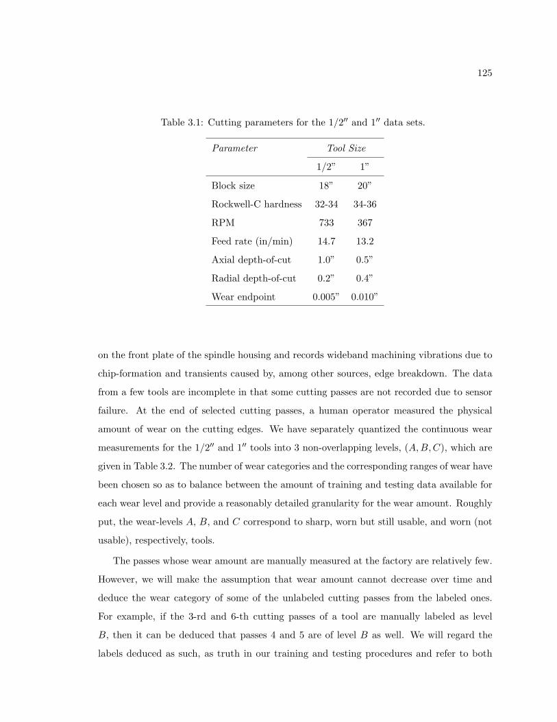
125
Table 3.1: Cutting parameters for the 1/2′′ and 1′′ data sets.
Parameter Tool Size
1/2” 1”
Block size 18” 20”
Rockwell-C hardness 32-34 34-36
RPM 733 367
Feed rate (in/min) 14.7 13.2
Axial depth-of-cut 1.0” 0.5”
Radial depth-of-cut 0.2” 0.4”
Wear endpoint 0.005” 0.010”
on the front plate of the spindle housing and records wideband machining vibrations due to
chip-formation and transients caused by, among other sources, edge breakdown. The data
from a few tools are incomplete in that some cutting passes are not recorded due to sensor
failure. At the end of selected cutting passes, a human operator measured the physical
amount of wear on the cutting edges. We have separately quantized the continuous wear
measurements for the 1/2′′ and 1′′ tools into 3 non-overlapping levels, (A,B,C), which are
given in Table 3.2. The number of wear categories and the corresponding ranges of wear have
been chosen so as to balance between the amount of training and testing data available for
each wear level and provide a reasonably detailed granularity for the wear amount. Roughly
put, the wear-levels A, B, and C correspond to sharp, worn but still usable, and worn (not
usable), respectively, tools.
The passes whose wear amount are manually measured at the factory are relatively few.
However, we will make the assumption that wear amount cannot decrease over time and
deduce the wear category of some of the unlabeled cutting passes from the labeled ones.
For example, if the 3-rd and 6-th cutting passes of a tool are manually labeled as level
B, then it can be deduced that passes 4 and 5 are of level B as well. We will regard the
labels deduced as such, as truth in our training and testing procedures and refer to both

126
Table 3.2: Wear categories and the corresponding ranges of wear, in thousands of an inch.
Wear Level Tool Size
1/2” 1”
A 0–2.4 0–4.9
B 2.5–4.9 5.0–9.9
C > 4.9 > 10
the manually examined cutting passes and the passes whose wear levels have been deduced
as labeled. The aforementioned assumption in some other cases limit the wear categories
that an unlabeled cutting pass might correspond to. Continuing with the example before,
if we also know that the 10-th pass is labeled as C, then passes 7 through 9 can only
be B or C, but not A. Such partial information is useful and automatically incorporated
into the system training via the EM algorithm and the left-to-right transition matrices (cf.
Section 3.3.2). Previous work [106] on steel milling showed that such full EM-style training
with unlabeled data is more efficient than the Viterbi-style approaches.
Training, Testing, and Cross-validation Divisions Both 1/2′′ and 1′′ data sets consist of
multiple tools. The 1/2” data set consists of enough tools so that separate training and
testing sets are constructed for the 1/2′′ task. The 1/2′′ training data set is also used in
a 3-fold cross-validation by leave-2-out for system development. The 1′′ data set consists
of fewer numbers of tools, so we have used it only in 6-fold cross-validation by leave-1-out
in our experiments in the 1′′ task.7 The various statistics for the 1/2′′ training and testing
data sets and the 1′′ data are provided in Table 3.3.
Baseline Tool-Wear Condition Monitoring System
We used the system described in Section 3.3.2 as our baseline tool-wear condition monitoring
system. To remind the reader, in this system, a meta-HMM over the whole cutting passes
7In one case, two tools are regarded as one for cross-validation purposes.
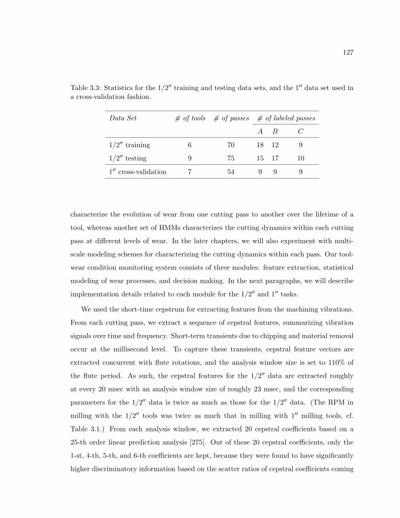
127
Table 3.3: Statistics for the 1/2′′ training and testing data sets, and the 1′′ data set used ina cross-validation fashion.
Data Set # of tools # of passes # of labeled passes
A B C
1/2′′ training 6 70 18 12 9
1/2′′ testing 9 75 15 17 10
1′′ cross-validation 7 54 9 9 9
characterize the evolution of wear from one cutting pass to another over the lifetime of a
tool, whereas another set of HMMs characterizes the cutting dynamics within each cutting
pass at different levels of wear. In the later chapters, we will also experiment with multi-
scale modeling schemes for characterizing the cutting dynamics within each pass. Our tool-
wear condition monitoring system consists of three modules: feature extraction, statistical
modeling of wear processes, and decision making. In the next paragraphs, we will describe
implementation details related to each module for the 1/2′′ and 1′′ tasks.
We used the short-time cepstrum for extracting features from the machining vibrations.
From each cutting pass, we extract a sequence of cepstral features, summarizing vibration
signals over time and frequency. Short-term transients due to chipping and material removal
occur at the millisecond level. To capture these transients, cepstral feature vectors are
extracted concurrent with flute rotations, and the analysis window size is set to 110% of
the flute period. As such, the cepstral features for the 1/2′′ data are extracted roughly
at every 20 msec with an analysis window size of roughly 23 msec, and the corresponding
parameters for the 1/2′′ data is twice as much as those for the 1/2′′ data. (The RPM in
milling with the 1/2′′ tools was twice as much that in milling with 1′′ milling tools, cf.
Table 3.1.) From each analysis window, we extracted 20 cepstral coefficients based on a
25-th order linear prediction analysis [275]. Out of these 20 cepstral coefficients, only the
1-st, 4-th, 5-th, and 6-th coefficients are kept, because they were found to have significantly
higher discriminatory information based on the scatter ratios of cepstral coefficients coming

128
0 2 4 6 8 10 12 14 16 18 200
0.005
0.01
0.015
0.02
0.025
0.03
0.035
0.04
0.045
cepstral coefficient
scatter ratio − ρ
Figure 3.4: The scatter ratios for the first 20 cepstral coefficients, calculated from the labeledcutting passes in the 1/2′′ training set.
from worn and not worn passes:
ρ ≡ (µ0 − µ1)2
σ20 + σ2
1
,
where µs and σ2s denote the sample mean and variance of the features coming from passes
labeled as worn (s = 0 corresponding to the wear categories A and B) and not worn (s = 1
corresponding to the wear category C). We have selected the 1-st, 4-th, 5-th, and 6-th
cepstral coefficients based on the scatter ratios estimated from the labeled passes in the
1/2′′ training data (cf. Figure 3.4). These choice of cepstral features are used for both 1/2′′
and 1′′ task experiments. Such a feature selection is not done separately for the 1′′ data,
since the 1′′ data are used in a cross-validation fashion, and it would not be fair. To minimize
the effects of tool-specific biases and accelerometer effects, cepstral mean subtraction has
been applied on a tool-by-tool basis as follows. The mean cepstral vector for each tool is
calculated by taking the sample mean of cepstral features coming from the first 3 passes of
that tool, if they are available. If not, the global mean of such first 3 passes across all tools
is used as the cepstral mean. This cepstral mean is subtracted from all features coming
from the corresponding tool.
The wear-level HMM characterizing the wear process from one cutting pass to another
129
has three states, one for each wear level (A, B, and C), and a left-to-right state-topology.
The initial wear probabilities and wear-transition probabilities are estimated by fitting a
Poisson model to the training passes with known wear labels. An initial probability distri-
bution over all wear categories is needed, because some of the tools in our data sets have
only their later passes recorded. The output distributions of this meta HMM are repre-
sented by HMMs characterizing the cutting dynamics within each pass. There are three
such HMMs, one corresponding to each wear category. Ergodic state transition topologies
have been chosen for these pass-level HMMs, based on both the pilot experiments and the
absence of any prior knowledge suggesting a left-to-right, or any other state topology.8 The
mixture of Gaussian distributions with diagonal covariance matrices are used to model the
state-conditional output distributions for the cepstral features. The number of states and
number of mixtures for these pass-level HMMs are determined via cross-validation, but
typically 4 states and 2 Gaussian components per state are used. The parameters of the
pass-level HMMs, namely initial state and state transition probabilities, and the Gaussian
mixture parameters, are jointly estimated from data using the EM algorithm which auto-
matically handles both the hidden states associated with unlabeled cutting passes and the
hidden states associated with the pass-level HMMs. The EM algorithm operates at two
levels on the composite model for each tool, consisting of the sequence of all cutting passes
from that tool. The resulting update equations for the parameters of each HMM associated
with a particular wear category is similar to the Baum-Welch updates in Section 2.6.3, but
the sufficient statistics from each cutting pass are also weighted by the a posteriori prob-
ability of the corresponding wear category for that cutting pass (which are calculated by
the forward-backward algorithm operating over the meta HMM). This training procedure is
initialized by setting the initial state and state transition probabilities of each wear HMM to
uniform distributions and their state-conditional output distributions to single-component
Gaussians as obtained by the k-means clustering of features coming from the labeled cut-
ting passes. The mixture splitting strategy uses 5 EM iterations after each split and 10 EM
8This is unlike steel milling where a left-to-right state topology was found to be successful for capturingthe distinct characteristics of machining vibrations at the entry to the piece and exit from the pieceregions [105].

130
iterations after the desired number of mixtures is reached.
During testing, the wear category for each cutting pass of a tool is predicted according
to the forward a posteriori probabilities in Equation 3.12. As mentioned before, these
forward a posteriori probabilities are calculated from the HMM forward algorithm, but by
using the cutting-pass likelihoods p(Yl|Wl = w)’s scaled by the sequence lengths Tl’s in the
natural logarithm domain. This normalization is also employed during training, when the a
posteriori wear probabilities for each cutting pass are calculated via the forward-backward
algorithm. In some of our experiments on the 1/2′′ testing set, the optional GLM posterior
correction is used. The GLM regression weights βw’s in Equation 3.11 are estimated using
the iteratively re-weighted least squares algorithm [188] via cross-validation on the training
data set. In the leave-k-out cross-validation with k = 2, k tools are set aside for testing
while the remaining tools are used to train the monitoring system, which is in turn used to
obtain the GLM features, the log-odds ratios (cf. Equation 3.11), for the k tools that were
set aside. By rotation, the features for all the tools appearing in the training data set are
obtained. The GLM regression weights are then estimated by the iteratively re-weighted
least squares algorithm over the labeled cutting passes. Since the GLM parameters are
estimated using the full training data set, the cross-validation on the same training set
results with the GLMs would result an overly optimistic performance estimate, and hence
an assessment on an independent testing set is necessary. As such, the GLMs are only used
in the 1/2′′ task but not in the 1′′ task, which does not have an independent testing set.
Software
We have used the software that we developed in MATLAB to perform our machine tool-wear
condition monitoring experiments.
3.4 Summary
In this chapter we have described the three applications (speech recognition, speaker ver-
ification, and machine tool-wear monitoring), which we will use in our experiments in the
later chapters to show the utility of developed tools and methods. For each application, we

131
gave a basic problem description, a baseline system architecture, and the specific tasks and
experimental paradigms for our tests, including details of training and testing procedures,
and data.

132
Chapter 4
MULTI-RATE HIDDEN MARKOV MODELS AND THEIR
APPLICATIONS
In this chapter, we will present multi-rate hidden Markov models (multi-rate HMMs), a
multi-scale generalization of HMMs for temporal processes with multi-scale dynamics and
dependence. A multi-rate HMM decomposes process variability into scale-based parts and
jointly models both the evolution within each scale-based part and interactions among scale-
based parts. While scale-based state sequences represent temporally changing properties
in each scale, there is also an observation sequence associated with each scale. Processes
involving multi-scale dynamics and long-term dependence are abundant [13, 90], and we will
present applications of multi-rate HMMs to wear process modeling for machine tool-wear
monitoring and acoustic modeling for speech recognition.
This chapter will start with a description of basic multi-rate HMMs and its modeling
assumptions. Next, we will present algorithms for solving probabilistic inference and pa-
rameter estimation problems of multi-rate HMMs. The basic multi-rate HMM architecture
is rather limited in a number of aspects, including the use of a time-invariant sampling
scheme for the multi-scale observation sequences and the restricted form of cross-scale de-
pendencies between scale-based parts. To address these deficiencies, we will introduce a
number of extensions to the basic multi-rate HMM architecture to allow for time-varying
sampling schemes and more direct cross-scale dependency schemes. Next, we will compare
multi-rate HMMs to HMMs and other multi-scale and related models previously proposed
in the literature. We will conclude this chapter with two pattern recognition applications
of multi-rate HMMs: first, machine tool-wear monitoring where multi-rate HMMs are used
for modeling of wear processes in titanium milling, and second, speech recognition where
multi-rate HMMs are used for multi- and variable-rate acoustic modeling of speech over
phone and syllable time scales.
133
4.1 Multi-rate HMMs
Multi-rate HMMs are a parsimonious statistical model for hierarchical modeling of processes
with multi-scale dynamics using scale-dependent state and observation sequences. Scales in
a multi-rate HMM are organized in a coarse-to-fine manner, allowing for efficient representa-
tion of both short- and long-term context simultaneously. In multi-rate HMMs, scale-based
state sequences characterize the non-stationary process dynamics within each scale-based
part, and scale-based observation sequences probe the process at the corresponding time
scales. Probabilistic dependencies across time and scale in multi-rate HMMs account for
both the intra-scale evolution within each scale-based part and inter-scale couplings between
scale-based parts.
More formally, there are K scales in a K-rate HMM, and each scale has its own obser-
vation and state sequences, {Sktk}Tk−1
tk=0 and {Oktk}Tk−1
tk=0 , respectively, where the superscript
k denotes the scale number, and Tk is the length of the observation sequence in the k-th
scale. We assume that scales are ordered from the coarsest k = 1 to the finest k = K, and
the k-th scale is Mk times faster than the (k − 1)-th scale, i.e. Tk = Mk Tk−1 for k > 1 (we
will later drop this restriction in Section 4.2). A multi-rate HMM characterizes the joint
distribution of state and observation sequences over all time scales as
p({O1
t1}, {S1t1}, . . . , {O
KtK}, {SK
tK})≡
K∏k=1
Tk−1∏tk=0
p(Sk
tk|Sk
tk−1, Sk−1btk/Mkc
)p(Ok
tk|Stk
)(4.1)
where Sk−1 is a null start state for the k-th scale; bxc denotes the greatest integer less
than or equal to x; and hence, btk/Mkc is the index of the observation in the (k − 1)-th
scale overlapping with the tk-th observation in the k-th scale. Parameters of a multi-
rate HMM consist of initial state distributions, p(Sk0 |S
k−10 ), state transition distributions,
p(Sk
tk|Sk
tk−1, Sk−1btk/Mkc
), and state-conditional observation distributions, p(Ok
tk|Sk
tk), for k=
1, . . . ,K. Similar to an HMM, a multi-rate HMM can accept discrete- or continuous-valued
observations, but in this thesis, we will focus on continuous-valued observations and model
the state-conditional observation distributions with mixture of Gaussian distributions.
A graphical model illustration of a 2-rate HMM appears in Figure 4.1, which clearly
illustrates the modeling assumptions behind multi-rate HMMs. The observations are inde-
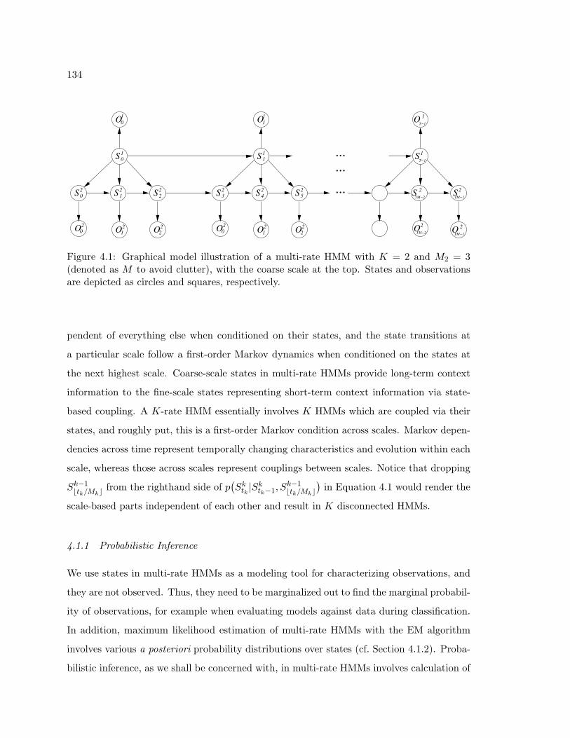
134
S 0 S S2 2 2
O20O O12 2 2
0O1
S10
1 2 S S S2 2 2
O20O O12 2 2
O1
S11
1
3 4...
...
...
1
5
S1
O
S2
O 2
2S
T−1
T−1
TM−1
TM−1O2
TM−2
TM−2
Figure 4.1: Graphical model illustration of a multi-rate HMM with K = 2 and M2 = 3(denoted as M to avoid clutter), with the coarse scale at the top. States and observationsare depicted as circles and squares, respectively.
pendent of everything else when conditioned on their states, and the state transitions at
a particular scale follow a first-order Markov dynamics when conditioned on the states at
the next highest scale. Coarse-scale states in multi-rate HMMs provide long-term context
information to the fine-scale states representing short-term context information via state-
based coupling. A K-rate HMM essentially involves K HMMs which are coupled via their
states, and roughly put, this is a first-order Markov condition across scales. Markov depen-
dencies across time represent temporally changing characteristics and evolution within each
scale, whereas those across scales represent couplings between scales. Notice that dropping
Sk−1btk/Mkc from the righthand side of p
(Sk
tk|Sk
tk−1, Sk−1btk/Mkc
)in Equation 4.1 would render the
scale-based parts independent of each other and result in K disconnected HMMs.
4.1.1 Probabilistic Inference
We use states in multi-rate HMMs as a modeling tool for characterizing observations, and
they are not observed. Thus, they need to be marginalized out to find the marginal probabil-
ity of observations, for example when evaluating models against data during classification.
In addition, maximum likelihood estimation of multi-rate HMMs with the EM algorithm
involves various a posteriori probability distributions over states (cf. Section 4.1.2). Proba-
bilistic inference, as we shall be concerned with, in multi-rate HMMs involves calculation of
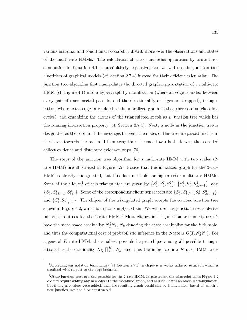
135
various marginal and conditional probability distributions over the observations and states
of the multi-rate HMMs. The calculation of these and other quantities by brute force
summation in Equation 4.1 is prohibitively expensive, and we will use the junction tree
algorithm of graphical models (cf. Section 2.7.4) instead for their efficient calculation. The
junction tree algorithm first manipulates the directed graph representation of a multi-rate
HMM (cf. Figure 4.1) into a hypergraph by moralization (where an edge is added between
every pair of unconnected parents, and the directionality of edges are dropped), triangu-
lation (where extra edges are added to the moralized graph so that there are no chordless
cycles), and organizing the cliques of the triangulated graph as a junction tree which has
the running intersection property (cf. Section 2.7.4). Next, a node in the junction tree is
designated as the root, and the messages between the nodes of this tree are passed first from
the leaves towards the root and then away from the root towards the leaves, the so-called
collect evidence and distribute evidence steps [76].
The steps of the junction tree algorithm for a multi-rate HMM with two scales (2-
rate HMM) are illustrated in Figure 4.2. Notice that the moralized graph for the 2-rate
HMM is already triangulated, but this does not hold for higher-order multi-rate HMMs.
Some of the cliques1 of this triangulated are given by{S1
0 , S20 , S
21
},{S1
0 , S11 , S
2M2−1
}, and{
S11 , S
2M2−1, S
2M2
}. Some of the corresponding clique separators are
{S1
0 , S21
},{S1
0 , S2M2−1
},
and{S1
1 , S2M2−1
}. The cliques of the triangulated graph accepts the obvious junction tree
shown in Figure 4.2, which is in fact simply a chain. We will use this junction tree to derive
inference routines for the 2-rate HMM.2 Most cliques in the junction tree in Figure 4.2
have the state-space cardinality N22N1, Nk denoting the state cardinality for the k-th scale,
and thus the computational cost of probabilistic inference in the 2-rate is O(T2N22N1). For
a general K-rate HMM, the smallest possible largest clique among all possible triangu-
lations has the cardinality NK∏K
k=1Nk, and thus the inference in a K-rate HMM takes
1According our notation terminology (cf. Section 2.7.1), a clique is a vertex induced subgraph which ismaximal with respect to the edge inclusion.
2Other junction trees are also possible for the 2-rate HMM. In particular, the triangulation in Figure 4.2did not require adding any new edges to the moralized graph, and as such, it was an obvious triangulation,but if any new edges were added, then the resulting graph would still be triangulated, based on which anew junction tree could be constructed.
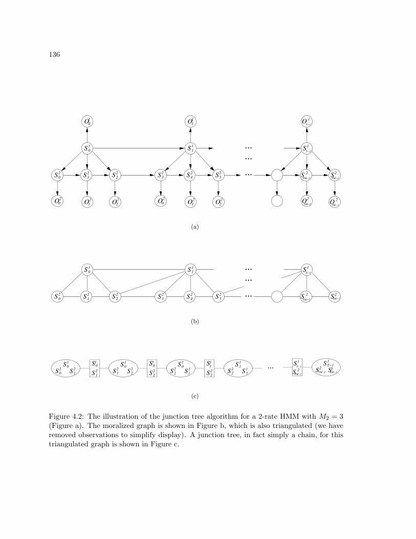
136
S 0 S S2 2 2
O20O O12 2 2
0O1
S10
1 2 S S S2 2 2
O20O O12 2 2
O1
S11
1
3 4...
...
...
1
5
S1
O
S2
O 2
2S
T−1
T−1
TM−1
TM−1O2
TM−2
TM−2
(a)
S 0 S S2 2 2
S10
1 2 S S S2 2 2
S11
3 4...
...
...
5
ST−1
1
S22STM−2 TM−1
(b)
S10S2
1S02
S21
S10
S2 S21 2
S10
S2 SS2
S0
22
... S1
S2S 2
ST−1
1T−1
TM−2 STM−2
TM−12
S1
S 2 SS2
S2
1
211
1
3
11S0
1 1
(c)
Figure 4.2: The illustration of the junction tree algorithm for a 2-rate HMM with M2 = 3(Figure a). The moralized graph is shown in Figure b, which is also triangulated (we haveremoved observations to simplify display). A junction tree, in fact simply a chain, for thistriangulated graph is shown in Figure c.

137
O(TKNK
∏Kk=1Nk
)computational cost, based on a junction tree for a K-rate HMM, which
is again a chain.
The inference over the junction tree consists of messages passed back and forth between
the cliques of the junction tree in the collect evidence and distribute evidence phases. We
have arbitrarily chosen the last clique in time{S1
T−1, S2TM−2, S
2TM−1
}as the root node,
and the messages propagate forward from the first clique{S1
0 , S20 , S
21
}during the collect
evidence phase and backward from the last clique{S1
T−1, S2TM−2, STM−1
}during the dis-
tribute evidence phase. We will refer to the collect evidence and distribute evidence phases
for the multi-rate HMMs as the forward and backward, respectively, passes to draw parallels
with the forward-backward algorithm of HMMs, which is widely understood. As is done
with the HMM forward-backward recursions in Section 2.6.1, we will recurse from separator
to separator rather than from clique to clique. This can lead to significant speedups, as
long as there are no variables that exist only in a clique, which is the case for the junction
tree in Figure 4.2. The goal of the inference routines presented below is to calculate the
marginal probability of observations and various a posteriori probabilities over states, which
will be needed for the parameter estimation of multi-rate HMMs (cf. Section 4.1.2). To sim-
plify the presentation we will consider the K = 2 case. The generalization to K > 2 is
straightforward. Even though there exist general purpose software implementations of the
junction tree algorithm such as [281] that can perform inference for the multi-rate HMM,
or a generic graphical model, we will explicitly derive the inference routines for the 2-rate
HMM, because significant speedups are possible from software implementations that are
tailored to a particular model. This was the case in our MATLAB implementation of the
inference in 2-rate HMMs, which we used in our tool-wear monitoring experiments.
To simplify equations, we will use the following notation. The long- and short-term
(k = 1 and k = 2, respectively) state and observation sequences in the 2-rate HMM will
be distinguished by the superscripts c (coarse) and f (fine), respectively. We assume that
the long-term chain is M times faster than the short-one, and the length of long-term
observation sequence is T . We also define,
Oc≤t ≡ {Oc
τ}tτ=0 , Oc
<t ≡ {Ocτ}
t−1τ=0 , and Oc
>t ≡ {Ocτ}
T−1τ=t+1 .
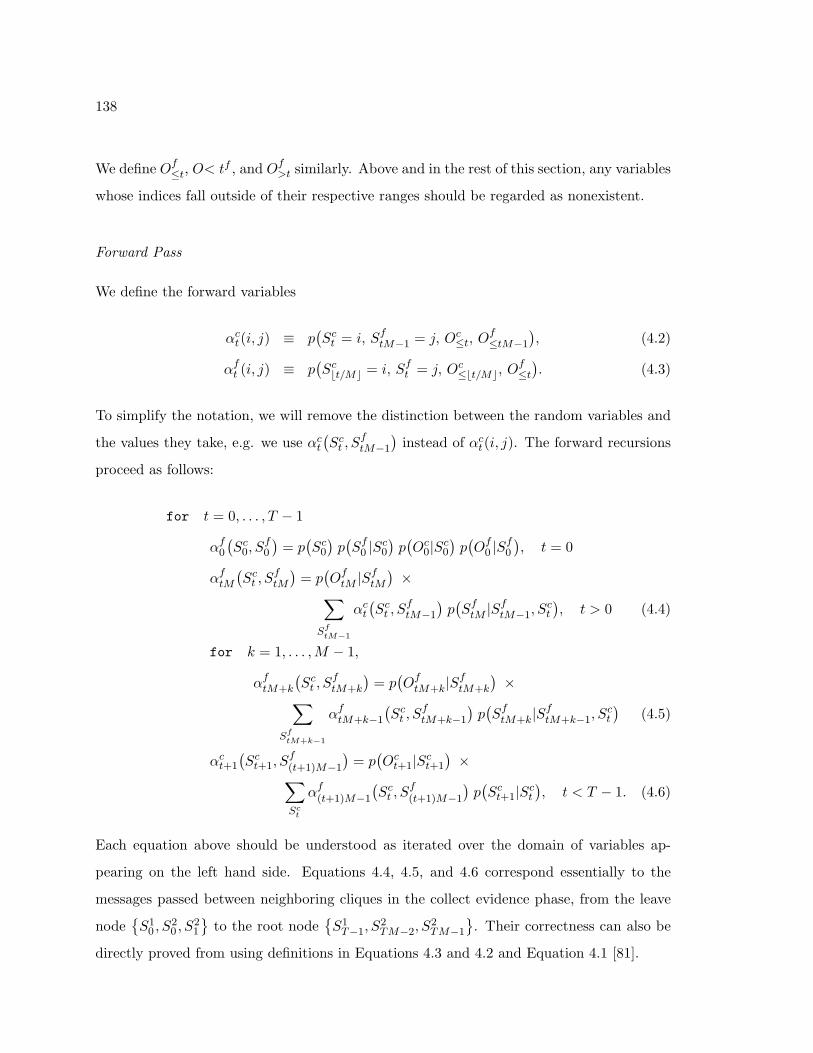
138
We define Of≤t, O< tf , and Of
>t similarly. Above and in the rest of this section, any variables
whose indices fall outside of their respective ranges should be regarded as nonexistent.
Forward Pass
We define the forward variables
αct(i, j) ≡ p
(Sc
t = i, SftM−1 = j, Oc
≤t, Of≤tM−1
), (4.2)
αft (i, j) ≡ p
(Scbt/Mc = i, Sf
t = j, Oc≤bt/Mc, O
f≤t
). (4.3)
To simplify the notation, we will remove the distinction between the random variables and
the values they take, e.g. we use αct
(Sc
t , SftM−1
)instead of αc
t(i, j). The forward recursions
proceed as follows:
for t = 0, . . . , T − 1
αf0
(Sc
0, Sf0
)= p(Sc
0
)p(Sf
0 |Sc0
)p(Oc
0|Sc0
)p(Of
0 |Sf0
), t = 0
αftM
(Sc
t , SftM
)= p(Of
tM |SftM
)×∑
SftM−1
αct
(Sc
t , SftM−1
)p(Sf
tM |SftM−1, S
ct
), t > 0 (4.4)
for k = 1, . . . ,M − 1,
αftM+k
(Sc
t , SftM+k
)= p(Of
tM+k|SftM+k
)×∑
SftM+k−1
αftM+k−1
(Sc
t , SftM+k−1
)p(Sf
tM+k|SftM+k−1, S
ct
)(4.5)
αct+1
(Sc
t+1, Sf(t+1)M−1
)= p(Oc
t+1|Sct+1
)×∑
Sct
αf(t+1)M−1
(Sc
t , Sf(t+1)M−1
)p(Sc
t+1|Sct
), t < T − 1. (4.6)
Each equation above should be understood as iterated over the domain of variables ap-
pearing on the left hand side. Equations 4.4, 4.5, and 4.6 correspond essentially to the
messages passed between neighboring cliques in the collect evidence phase, from the leave
node{S1
0 , S20 , S
21
}to the root node
{S1
T−1, S2TM−2, S
2TM−1
}. Their correctness can also be
directly proved from using definitions in Equations 4.3 and 4.2 and Equation 4.1 [81].

139
Backward Pass
We define
βct
(Sc
t , SftM−1
)≡ p
(Oc
>t, Of>tM−1 | S
ct , S
ftM−1
),
βft
(Scbt/Mc, S
ft
)≡ p
(Oc
>bt/Mc, Of>t | Sc
bt/Mc, Sft
).
The backward recursions proceed as follows:
for t = T − 1, . . . , 0
βfTM−1
(Sc
T−1, SfTM−1
)= 1, t = T − 1
βf(t+1)M−1
(Sc
t , Sf(t+1)M−1
)=∑Sc
t+1
p(Sc
t+1|Sct
)p(Oc
t+1|Sct+1
)×
βct+1
(Sc
t+1, Sf(t+1)M−1
), t < T − 1 (4.7)
for k = 2, . . . ,M
βf(t+1)M−k
(Sc
t , Sf(t+1)M−k
)=∑
Sf(t+1)M−k+1
βf(t+1)M−k+1
(Sc
t , Sf(t+1)M−k+1
)×
p(Sf
(t+1)M−k+1|Sf(t+1)M−k, S
ct
)p(Of
(t+1)M−k+1|Sf(t+1)M−k+1
)(4.8)
βct
(Sc
t , SftM−1
)=∑Sf
tM
p(Sf
tM |SftM−1, S
ct
)p(Of
tM |SftM
)×
βftM
(Sc
t , SftM
), t > 0 (4.9)
Again, each equation is iterated over the domain of variables appearing on the left hand
side. Equations 4.7, 4.8 and 4.9 essentially correspond to the messages passed during the
distribute evidence phase, from the root node{S1
T−1, S2TM−2, STM−1
}to the leave node{
S10 , S
20 , S
21
}. Their correctness can again be directly proven using the multi-rate HMM
factorization in Equation 4.1 [81].
Marginal Likelihood and Hidden State Posteriors
The marginal likelihood of observations O ≡ {{Oct}, {O
ft }} can be calculated from the
forward variable αfTM−1(S
cT−1, S
fTM−1) by integrating out the hidden states
p(O) =∑
ScT−1,Sf
TM−1
αfTM−1(S
cT−1, S
fTM−1)
140
which directly follows from the definition in Equation 4.3. We will need the following a
posteriori distributions for the parameter estimation of multi-rate HMMs with the EM
algorithm:
γccft
(Sc
t−1, Sct , S
ftM−1
)≡ p
(Sc
t−1, Sct , S
ftM−1|O
), (4.10)
γcfft
(Scbt/Mc, S
ft−1, S
ft
)≡ p
(Scbt/Mc, S
ft−1, S
ft |O
). (4.11)
(We will generally use γ to denote a posteriori distributions and superscripts such as ccc and
ccf to denote the collections of the hidden variables associated with these distributions.)
These a posteriori distributions are obtained from the forward and backward variables as
follows,
γccft
(Sc
t−1, Sct , S
ftM−1
)∝ αf
tM−1
(Sc
t−1, SftM−1
)p(Sc
t |Sct−1
)×
p(Oc
t |Sct
)βc
t
(Sc
t , SftM−1
)γcff
tM
(Sc
t , SftM−1, S
ftM
)∝ αc
t−1
(Sc
t , SftM−1
)p(Sf
tM |SftM−1, S
ct
)×
p(Of
tM |SftM
)βf
tM
(Sc
t , SftM
)γcff
tM+k
(Sc
t , SftM+k−1, S
ftM+k
)∝ αf
tM+k−1
(Sc
t , SftM+k−1
)p(Sf
tM+k|SftM+k−1, S
ct ) ×
p(OftM+k|S
ftM+k) β
ftM+k(S
ct , S
ftM+k).
by again making use of the multi-rate HMM independence assumptions.
We finish this section with two comments. First, the overall computational cost of
inference in the 2-rate HMM is O(TNcN2f ), which compares favorably to O(TN2
cN2f ) com-
putational cost as it would be the case if the inference was performed by emulating a 2-rate
HMM with an HMM which represents the meta-space of fine and coarse state sequences,
and by invoking the HMM forward-backward algorithm. Second, it is easy to modify the
forward pass described in Section 4.1.1 to obtain the Viterbi state sequence, the state se-
quence having the highest a posteriori probability given the observations, similar to the way
we modified the HMM forward algorithm for the Viterbi algorithm in Section 2.6.2.
4.1.2 Parameter Estimation
In this section, we will describe an EM algorithm for the maximum likelihood parameter
estimation of multi-rate HMMs. Since the states in multi-rate HMMs are hidden, the direct
141
maximization of the incomplete data likelihood is mathematically intractable, hence the use
of the EM algorithm. The parameters of the multi-rate HMM consists of the initial state
and state transition probabilities associated with scale-based chains, the parameters asso-
ciated with the state-conditional observation densities which we assume to be represented
by mixture of Gaussian distributions. Multi-rate HMMs also involve structural parameters
such as the hidden states cardinalities, state-transition topologies, and number of mixtures,
and diagonal vs. full-covariance modeling in the state-conditional observation distributions.
Determining structural parameters is a model selection problem, and we will deal with them
separately in our applications in Section 4.3. In this section, we will only consider the 2-rate
HMM, but the generalization to higher-order models is straightforward. We will assume
that there is only one example in the training data set with the observation sequences
O ≡ {{Oct}, {O
ft }} and the associated unobserved state sequences S ≡ {{Sc
t }, {Sft }}. The
extension to the multiple training examples case is trivial.
The parameters of the coarse-rate side of the 2-rate HMM consist of initial state distri-
bution πcs ≡ p(Sc
0 = s), state transition probabilities acss′ ≡ p(Sc
t = s|Sct−1 = s′), and the
mixture weights, means, and covariances, {αcms, µ
cms,Σ
cms}, associated with the mixture of
Gaussian output distributions:
p(Oct = oc|Sc
t = s) =Mc∑
m=1
αcms N (oc;µc
ms,Σcms), (4.12)
Mc denoting the number of mixture components. The fine-rate counterparts of these pa-
rameters are given by πfssc ≡ p
(Sf
0 = s|Sc0 = sc
), af
ss′sc = p(Sf
t = s|Sft−1 = s′, Sc
bt/Mc = sc),
and {αfms, µ
fms,Σ
fms}, with obvious notation.
The EM algorithm works by iteratively maximizing the expected complete data like-
lihood based on the multi-rate HMM factorization in Equation 4.1 with respect to the
aforementioned 2-rate HMM parameters, which we collectively denote by θ:
θ(i) ≡ argmaxθ{Eθ(i−1) [log pθ(S,O|O)]} (4.13)
where i denotes the iteration number, and θ(i) denotes the parameters from the i-th iteration.
The solution to Equation 4.13 is easily be found by differentiation, giving the following
142
updates for the initial state and state-transition probabilities:
πcs = γc
0(s), acss′ =
∑T−1t=1 γcc
t (s′, s)∑Tt=1 γ
ct (s′)
,
πfssc = γcf
0 (sc,s)γc0(sc) , af
ss′sc =∑TM−1
t=1 γcfft (sc, s′, s)∑TM−1
t=1 γcft (sc, s′)
where we have dropped the iteration number over parameters to simplify the notation; the
a posteriori distribution γcfft is defined in Equation 4.10, and the a posteriori distribu-
tions γct (s) ≡ p
(Sc
t = s|O), γcc
t (s′, s) ≡ p(Sc
t−1 = s′, Sct = s|O), and γcf
t (sc, s) ≡ p(Scbt/Mc =
sc, Sft = s|O
), which are easily obtained from the a posteriori distributions in Equation 4.10
and 4.11 through marginalization. These and other a posteriori distributions below appear-
ing in the EM algorithm updates are calculated using the parameters from the previous
iteration and the probabilistic inference algorithm in Section 4.1.1. The update equations
for the mixture weights, means, and covariance matrices are also found by differentiation,
which are similar to the Baum-Welch updates in Equations 2.51– 2.53. For the coarse-rate
mixture parameters, they take the form
αcms =
∑T−1t=0 ζc
t (m, s)∑T−1t=0 γc
t (s)(4.14)
µcms =
∑T−1t=0 ζc
t (m, s) Oct∑T−1
t=0 ζct (m, s)
(4.15)
Σcms =
∑T−1t=0 ζc
t (m, s) Oct
(Oc
t
)>∑T−1t=0 ζc
t (m, s)− µc
ms
(µc
ms
)> (4.16)
where ζct (m, s) is the a posteriori joint state-mixture probability
ζct (m, s) ≡ p
(Sc
t = s, Lct = m|O
)= γc
t (s) γct (m|s);
Lct denotes the unobserved mixture variable in Equation 4.12; and, γc
t (m|s) ≡ p(Lct = m|Oc
t )
is the a posteriori mixture probability, calculated according to Equation 4.12 using the
parameters from the (i− 1)-th iteration. The update equations for the mixture parameters
associated the fine-rate chain are identical to Equations 4.14, 4.15, and 4.16 with obvious
modifications.
143
4.1.3 Comparisons to HMMs and Previous Work
In this section, we will compare multi-rate HMMs to HMMs and various multi-scale and
other related models for representing multi-scale processes.
Comparison to HMMs
An HMM in theory can represent any state-space model by appropriate grouping of the
possibly multiple state and observation sequences of the original model into single state
and observation sequences. As such, an HMM can be constructed to emulate a multi-rate
HMM as follows. Additional states between the consecutive states in the coarser scales are
introduced so that each scale-based state sequence involves the same number of states as
the finest-scale state sequence. The Cartesian product of the states within the same time
frame are then taken to construct the state sequence of the emulating HMM. The state-
transition topology in the emulating HMM is restricted such that the component states
corresponding to coarser scales in the multi-rate HMM cannot change their value at every
time frame. Similarly, the output distributions of this HMM are arranged so that not every
product-state configuration emits all scale-based observations corresponding to the original
multi-rate HMM, at each time frame. The product-state at a particular time emits an
observation for a particular scale only if this observation is emitted at the corresponding
scale before the inclusion of additional states. The resulting model is not really an HMM as
described in Section 2.6 due to its special emitting structure, and the state transition and
state-conditional observation distributions need to be specially parameterized to be able
to replicate the state transition and observation distributions of the multi-rate HMM. The
resulting product state space is exponential in the number of scales. The consequences of
these changes are two fold. During decoding, the product state space results in an expo-
nentially higher cost of inference due to the fact that there are exponentially many states
and that the cost of inference in an HMM is quadratic in the number of states (cf. Sec-
tion 2.6.1). During training, the closed-form parameter updates cannot be obtained for the
state-transition probabilities of the emulating HMM, since they are algebraically tied to
each other in the HMM parameterization. Relaxing the algebraic constraints in the param-
144
eterization results in closed-form updates, but the number of parameters is exponentially
more, causing estimation problems.
Above we constructed an HMM to emulate a given multi-rate HMM. In practice, HMMs
with a hierarchical structure are also used to represent complex but hierarchical systems
such as language and speech. In state-of-the-art speech recognition systems, in particular
the one described in Section 3.1, acoustic state space is hierarchically organized from words
to phones to sub-phones. HMM-based acoustic models apply such hierarchical partitioning
to only states, as there is a single feature sequence emitted from the sub-phone states at the
finest scale of hierarchy. Such a hierarchical organization of states is primarily for purposes
of parameter estimation; and, little of the hierarchical structure is actually incorporated into
the model, though it is possible to do so. There are also multi-stream approaches to speech
recognition where multiple sequences of features are extracted either from different informa-
tion sources such as audio and video, or from the same acoustic signal using different signal
processing techniques. These feature sequences in many cases correspond to different time
scales. For example, in audio-visual speech recognition, the visual features extracted from
the video depicting speaker’s mouth are on average 50% slower than the spectral features
extracted from the accompanied audio signal [204]; and, in multi-band and tandem speech
recognition systems, features extracted from a mix of windows such as TRAPS from 500
msec windows and cepstral features from 25 msec windows typically correspond to different
time scales. In speech recognition systems, such multi-scale feature sequences are typically
handled by oversampling slower feature sequences, concatenating them with the faster fea-
ture sequences, and plugging the concatenated features as the observations into an HMM,
the so-called feature concatenation approach. When oversampled features extracted from
longer time windows are used in an HMM, they violate the HMM independence assumptions
more severely, and, in practice, a tweak factor is employed to downscale state-conditional
observation probabilities. Such downscaling essentially amounts to ignoring some of the
consecutive observation vectors which are expected to be highly correlated and receive simi-
lar probabilities. The violation of the HMM independence assumptions by the oversampled
feature sequences is not necessarily bad for classification, but in practice it is usually so (see
the experiments in Section 4.3), and such an oversampling results in poorer classification
145
performance and confidence estimation due to, roughly speaking, counting the evidence
from coarser scales multiple times due to oversampling .
Overall, we identify three main limitations of HMMs for characterizing multi-scale pro-
cesses, which, as compared to multi-scale modeling approaches, result in higher cost of
probabilistic inference, surfeit of parameters, overconfident classification decisions, and dif-
ficulties in extracting long-term structure from data. First, HMMs represent the underlying
state of the process by a single-component state variable, and the representation of compos-
ite state structures requires assigning a unique state to each possible state configuration.
The resulting exponential state space increases both the computational cost of inference
(quadratic in the cardinality of states) and the number of free parameters, making param-
eter estimation from scarce training data unreliable. Such parameter estimation problems
are particularly relevant to one of our applications, machine tool-wear monitoring where
the data is very sparse. Second, HMMs represent the observations from a process by a
single observation sequence, which makes it difficult to incorporate multi-scale observation
sequences into the HMM framework. Oversampling observations from coarser time scales
introduces redundancy and skews posterior estimates by overcounting, which needs to be
artificially handled by downscaling likelihood scores in general. Third, HMMs propagate
context information between the past and future observations, {Oτ}t−1τ=0 and {Oτ}T−1
τ=t , re-
spectively, via an information bottleneck, St, which can encode at most log2 |S| for St ∈ S,
bits of information since states constitute a first-order Markov chain. As the time lag be-
tween past and future increases, future becomes independent of past exponentially fast for
a large class of Markov chains, in particular those with an ergodic topology [27, 132]. Even
though structural constraints in the state transitions can be used to propagate long-term
context information to some degree, this approach requires a very large state space for long
sequences, making HMMs problematic for representing long-term context information.
Comparison to Previous Work in Multi-scale Modeling
In previous work, multi-scale models have appeared in many different facets of signal pro-
cessing and statistical modeling [266]. Some representative examples from the literature in-
146
clude hierarchical HMMs [103, 200], two-dimensional multi-resolution HMMs [179], hidden
Markov trees [78, 221], multi-resolution auto-regressive models [23, 192], multi-scale linear
dynamic systems [69], and multi-scale Markov random fields [183]. Among these models the
hidden Markov trees (used for wavelet-based signal recovery from noise [78]) and hierarchi-
cal HMMs (used for modeling English text and cursive handwriting [103], DNA motifs [200],
and robot navigation [255]) are most similar to the multi-rate HMMs developed in this the-
sis. In both hidden Markov trees and hierarchical HMMs, scale-based state and observation
sequences are organized in a hierarchical manner. While the tree-structured Markov depen-
dencies across scales characterize the coarse-to-fine inter-scale dynamics, Markov dependen-
cies within each state sequence model intra-scale process dynamics. The hidden Markov
trees and hierarchical HMMs differ from each other in their deterministic vs. stochastic
alignment of scale-based state sequences with each other. In hidden Markov trees, a coarser
scale state is aligned with a fixed number of the next-finest-scale states, whereas in hierarchi-
cal HMMs this restriction is avoided, and the alignment is formulated probabilistically. The
stochastic alignment case is exactly analogous to the stochastic segment model extension
of HMMs [213], in which the hidden states emit a random length sequence of observations
instead of a single observation.
The multi-rate HMMs have similarities to and differences from the hidden Markov trees
and the hierarchical HMMs. Similar to the either model, the multi-rate HMM characterizes
the inter-scale dependencies by tree-structured coarse-to-fine Markov dependencies across
scale and intra-scale temporal dependencies by first-order Markov dependencies across time.
In both multi-rate HMMs and hidden Markov trees, the alignment between scale-based se-
quences, i.e. observations at a finer scale corresponding to an observation at a coarser scale,
is formulated deterministically, which is unlike hierarchical HMMs where the alignment is
stochastic. The extension to probabilistic alignment in multi-rate HMMs and hidden Markov
trees is obvious, and in the next section, we will partially drop the fixed alignment assump-
tion in multi-rate HMMs. The main difference of multi-rate HMMs from hidden Markov
trees and hierarchical HMMs is that both of the latter models assume a tree-structured data
generation process where state and observation variables corresponding to a given time scale
are independent of their far distance relatives (that do not overlap with the same coarse

147
observation) conditional on their coarser ancestor state variables. Conditioning on coarse-
scale states in these two models partitions the state sequence at a given scale into islands of
Markov chains, each overlapping with a particular coarse state. This is unlike the multi-rate
HMMs where each scale-based state sequence constitutes a Markov chain even if conditioned
on higher-order scale states. Another difference of the multi-rate modeling framework de-
veloped in this thesis is an option for characterizing richer cross-scale interactions, as will
be described in the next section. In addition to state-based dependencies between scale-
based parts, we will model residual cross-scale observation dependencies not captured by
indirect state coupling and modify the state-conditional observation distributions to take
the higher-level context into account.
The coupling of state chains in the multi-rate HMM is similar to the coupled HMMs,
also known as the multi-stream coupled HMMs or simply multi-stream models in the speech
recognition literature, which use inter-stream Markov dependencies to couple two same-rate
hidden Markov models [48, 52, 94, 242, 209]. However, unlike the multi-rate HMMs, coupled
HMMs are inherently single-rate and do not effectively model long-range dependencies and
redundancy when used for modeling feature sequences corresponding to different time scales.
In passing, we note that all of the multi-scale models mentioned above assume a fixed
number of scales, which make them less powerful than the stochastic context-free grammars
in terms of their expressive power [200], though they are more powerful than tree-based
static models such as [71, 193] that assume fixed-length observation sequences. In addition,
finite state transducers [198] that are hierarchically organized are essentially multi-rate in
the state space.
4.2 Multi-rate HMM Extensions
The basic multi-rate HMMs introduced in Section 4.1 are somewhat restricted in charac-
terizing interactions between scale-based parts, and in this section, we will introduce two
extensions to relax these restrictions. The first extension concerns the multi-rate HMM’s
assumption that a fixed sampling ratio exists between the scale-based observation sequences,
and we will drop this assumption to allow for time-varying sampling rates between scale-
148
based observation sequences. The second extension concerns the assumption that when
conditioned on their hidden states observations are independent of everything else, in par-
ticular observations and states from coarser time scales. Thus, the scale-based observation
sequences interact with each other only indirectly via hidden states. We will introduce
additional direct dependencies on finer scales from the coarser ones to capture any de-
pendencies not captured by indirect state coupling. To simplify the presentation, we will
introduce these extensions using 2-rate HMMs, and the generalization of these methods to
higher-order multi-rate HMMs should be obvious.
4.2.1 Time-varying Sampling Rates in Multi-rate HMMs
In the multi-rate HMMs described in Section 4.1, we have assumed that each observation
and state at the scale k covers a fixed number Mk of observations and states at the next
finest scale, the scale (k−1). A fixed sampling rate ratio between the scale-based sequences
implicitly assume that observations in each scale uniformly cover the process over time and
that the state at the k-th scale can only change its value only after Mk state transitions
at the (k − 1) scale. Imposing such a fixed sampling rate ratio between the scale-based
sequences might not make sense for modeling phenomena that show large variations in
duration such as phones in speech recognition. For example, one of our applications of the
2-rate HMMs is to jointly model phones and sub-phonetic variability in acoustic modeling
of speech. In this application, the coarse and fine time scales characterize phones and sub-
phones, respectively. The phone durations in English range, nominally, from 10− 30 msecs
for stop consonants to 100 − 150 msecs for vowels, and a time-invariant sampling scheme
at the coarse scale might not be sufficiently detailed to resolve phonemes with very short
duration. In addition, for pattern recognition problems, a variable-rate signal analysis might
also be desirable, as it can tailor the analysis to focus more on information-bearing regions
such as phone transitions in speech recognition, as opposed to giving uniform emphasis over
the signal space. Variable-rate coding techniques are already in use in audio and image
coding [118, 83], and the variable-rate feature extraction methods have also been found
useful in speech recognition, especially for noisy speech, e.g. [53, 222, 6].
149
To temporally adapt the resolutions of both modeling units and signal analysis, we
extend the basic multi-rate HMM paradigm in Section 4.1 to allow for time-varying sampling
rates in the scale-based state and observation sequences. In this variable-rate extension of
multi-rate HMMs, the number of observations and states at a scale corresponding to each
observation or state at the next coarsest scale are allowed to temporally vary. For example,
the original 2-rate factorization which assumes a fixed sampling ratio, M ,
p({O1
t1}, {S1t1}, {O
2t2}, {S
2t2})≡
T1−1∏t1=0
p(S1
t1 |S1t1−1
)p(O1
t1 |S1t1
)×
(t1+1)M−1∏t2=t1M
p(S2
t2 |S1t1 , S
2t2−1
)p(O2
t2 |S2t2
)(4.17)
is modified to
p({O1
t1}, {S1t1}, {O
2t2}, {S
2t2} | {M
1t1})≡
T1−1∏t1=0
p(S1
t1 |S1t1−1) p
(O1
t1 |S1t1
)×
l(t1)+M1t1−1∏
t2=l(t1)
p(S2
t2 |S1t1 , S
2t2−1
)p(O2
t2 |S2t2
)(4.18)
where M1t1 denotes the number of observations at the fine scale (k = 2) overlapping with the
t1-th observation in the coarse scale (k = 1), and l(t1) denotes the starting index for these
overlapping fine scale observations. Notice that we necessarily have l(t1) =∑t1−1
τ1=0M1τ1
and T2 =∑T1−1
t1=0 M1τ1 in the variable-rate factorization. Setting M1
t1 = M for all t1 in
Equation 4.18 recovers the original fixed-rate factorization in Equation 4.17.
In the variable-rate factorization of Equation 4.18, we have assumed that sampling
rates {M1t1} are given, specified as input, and not modeled. The reason for this is that
our variable-rate sampling framework is partially motivated to focus on interesting regions
over the signal space, and such regions are determined during signal processing stage when
selecting coarse-scale features, and hence {M1t1}. For example, in Section 4.3.2, we will use
the variable-rate model in Equation 4.18 for acoustic modeling of speech at two time scales,
and the temporal resolutions of features and modeling units at the coarse scale are selected
to focus on transition regions where the extracted features tend to vary a lot from one
frame to the next. It is straightforward to make M1t1 random as in hierarchical HMMs [103]
150
and stochastic segment models [214], as we will describe next, but the cost of probabilistic
inference is higher, and it is not explored in this work. We note that the implementation of
such extensions is particularly straightforward in the graphical modeling framework.
The time-variable-rate extension of multi-rate HMMs in Equation 4.18 is identical to hi-
erarchical HMMs except the conditioning of fine-scale states at the coarse sampling bound-
aries on the previous fine-scale states: in the multi-rate HMMs, S2l(t1) is conditioned on
S1l(t1)−1 (cf. Equation 4.18), whereas in the hierarchical HMMs it is not (cf. Section 4.1.3). In
spirit, the time-varying extension in Equation 4.18 is also close to segment models [214] and
variable-duration HMMs [177]. In stochastic segment models, each state emits a sequence of
observations rather than a single observation, which are then jointly modeled by, for exam-
ple, a trajectory model [168]. The variable-duration HMMs are a special case of stochastic
segment models, where the emitted observation sequence is assumed to i.i.d. conditional
on the emitting state. The variable-rate extension in Equation 4.18 differs from these ex-
tensions of HMMs in that in both stochastic segment models and variable-duration HMMs,
each emitted observation sub-sequence is generated from the same hidden state, whereas in
the variable-rate extension, the fine-scale observation sub-sequence {O2t2}
l(t1)+M(t1)−1t2=l(t1) cor-
responding to each coarse scale observation is not assumed to be generated from the same
state.
4.2.2 Cross-scale Observation and State Dependencies
In the multi-rate HMMs described in Section 4.1, interactions between scale-based parts
are modeled by, roughly speaking, first-order Markov dependencies across scale. The state
transitions occurring at a particular scale are dependent on the state variable at the next
coarsest scale, the only mechanism via which the scale-based parts interact. Each scale-
based observation sequence is independent of the scale and observation sequences at other
scales, in particular those at coarser scales, once conditioned on its own state sequence. Our
goal in this section is to relax this independence assumption and allow for richer dependen-
cies between scale-based parts, to fine observations from coarser states and observations.
The reasons for considering such dependencies are many fold.
151
First, there might exist dependencies between scale-based observation sequences which
are not captured by indirect hidden state coupling alone. For example, it has been observed
that large/small values of wavelet coefficients of real world signals tend to propagate across
scales [78], and such persistence properties of the scale-based feature sequences might not
be captured by indirect state coupling. In addition, in pattern classification problems,
such direct cross-scale observations dependencies, if chosen according to a discriminative
criterion (see Section 5.5 for such a method within the context of multi-stream coupled
HMMs) might provide better discrimination between states. Second, the state space of the
multi-rate HMM is factored over scales, and the collection of scale-based state variables
at a given time slice provides a hierarchical representation of the process state. Yet, the
individual states in this factored representation might fail in representing long-term trends,
or phases in the process, depending on what each state sequence represents. Conditioning
finer observations on coarser scales in addition to the state at its own scale can provide an
effective way to incorporate long-term contexts for characterizing short-term observational
variability, for example, conditioning on suprasegmental effects such as syllable stress and
structure to resolve some of the acoustic variability at phone level in speech recognition.
Third, direct dependencies from coarser states and observations to the fine-scale observations
can make coarser scales more effective in the decision making process. The reason for this
is that in the factorization of Equation 4.1, each scale contributes to the joint probability
roughly proportional to its sequence length, and in this sense, the coarser scales are at a
disadvantage. Fourth, the temporal detail of the coarse-scale modeling units, i.e. states, are
usually much less than those of the finer scales. For example, in a particular experiment in
the 2-rate acoustic modeling of speech (cf. Section 4.3.2), we only had about 100 distinct
coarse-scale states to acoustically represent every possible word in English, as compared to
about 5, 000 states in the fine scale. As such, coarse-scale states and observations are much
broader, and by themselves, they do not provide enough granularity to distinguish between
different words. However, by direct conditioning of finer observations, which contribute
most to probabilities, on the coarser states and observations, coarse scales might have a
bigger impact on the probability scores and hence recognized units in a pattern classification
problem.

152
In this section, we will present two schemes of cross-scale dependencies: from coarser
observations to finer observations, and from coarser states to finer observations. We will
introduce these extensions with the framework of mixture of Gaussian output distributions
(cf. Equation 4.12):
p(Ok
t = o|Skt = s
)=
Mk∑m=1
αkms N
(o;µk
ms,Σkms
), (4.19)
where {αkms, µ
kms,Σ
kms} are the usual Gaussian mixture parameters associated with the
scale k, and Mk denotes the number of mixture components, not to be confused with M1t1
in Equation 4.18, denoting the sampling rates.
Cross-scale Observation Dependencies
An obvious choice to characterize dependencies between multi-scale observations is a multi-
resolution vector auto-regressive process [23]. We model that the observation Okt at scale
k and time t is dependent on the observations at coarser scales according to the following
linear Gaussian model
Oktk
=k−1∑p=1
Akp O
pbtkcp + etk (4.20)
conditional on the hidden state, say s, and mixture component, say m, of the Oktk
. In
Equation 4.20, Akp are the regression matrices, btkcp for p > k denotes the index of the
observation at the p-th scale covering the tk-th observation at the k-th scale, and etk is
white Gaussian noise, etk ∼ N(µk
ms,Σkms
)(see Equation 4.19). Including the auto-regressive
cross-scale observation dependencies alters the multi-rate factorization in Equation 4.1 by
replacing the original output distribution p(Ok
tk|Stk
)with an output distribution p
(Ok
t |Skt =
s,Ok−1btkck−1
, . . . , O1btkc1
), which is identical to the Gaussian mixture model in Equation 4.19
but with the new regressed means:
µkms | O ≡ µ
kms +
k−1∑p=1
Akp Obtkcp . (4.21)
Such dependency schemes will be explored in Chapter 5 for acoustic modeling based on
multi-stream coupled HMMs. The maximum likelihood parameter estimation of the auto-
regressive output distributions is straightforward, but an important modeling question is
153
what the granularity of regression matrices Apk should be. In Equation 4.21, we have assumed
that they are globally tied across all states and mixtures at a particular scale, which might
not be sufficient to capture any interesting structure from data. On the other hand, choosing
a different regression matrix for each state s and mixture m is likely to lead to estimation
problems for large-dimensional observations. A tying approach similar to the one used for
the clustering of triphone states in speech recognition could be necessary.
Cross-scale State Dependencies
In this section, we will introduce parsimonious hierarchical modeling schemes for the depen-
dence of finer scale observations on coarser states, assuming a mixture of Gaussian output
distributions model (cf. Equation 4.19). In this mixture model, dependence on coarser
states can simply be accomplished by conditioning the mixture parameters associated with
the fine scale on coarser states as well, but such an approach can dramatically increase the
total number of mixture components and scarcely partition the training data for reliable es-
timation of resulting mixtures. Instead, we look for more parsimonious and economic ways
of conditioning observational variability on coarser scales. The approach that we take is to
separately parameterize the effect of each source of variability (a state at a particular scale)
on the output distribution. The advantage of such a separation is that it increases the total
number of parameters additively on the scale-based state cardinalities, and yet it allows
for the construction of multiplicatively many output distributions. This idea is popularly
used in speech recognition to separate speech and speaker related factors in acoustic fea-
ture vectors for the adaptation of a speaker-independent recognition model to a particular
speaker [176, 8]. It is also similar to the bilinear model in [254] to separate the style and
context of handwritten images. We will illustrate our proposals for the extended cross-scale
state dependencies using the 2-rate HMM where the fine-scale observation densities will
be conditioned on the states at both scales, i.e. the output distribution p(O2
t |S2t
)in the
original 2-rate HMM factorization of Equation 4.17 is replaced by the output distribution
p(O2
t |S2t , S
1bt/Mc
).
The basic idea behind our proposals is to separately parameterize the effects of fine
154
and coarse states (S2t and S1
bt/Mc, respectively) on the fine observations (O2t ). One way to
achieve this separation is to adapt the fine-state dependent mean vectors in Equation 4.19
by a coarse-state dependent linear transformation:
p(O2
t = o | S2t = s, S1
bt/Mc = s1)
=M2∑
m=1
α2ms N
(o; As1µ2
sl + bs1 , Σ2ms
)(4.22)
where bs1 and As1 denote the bias and transformation matrix, respectively, of the transfor-
mation. This adaptation method is known as the maximum likelihood linear regression in
speech recognition literature and commonly used for speaker adaptation [176]. The maxi-
mum likelihood estimation of the linear transformation parameters bs1 and As1 is straight-
forward. An alternative to the model-space adaptation in Equation 4.22 is the following
feature-space adaptation where the modeling space of the fine observations is dynamically
changed according to the coarse states:
p(O2
t = o | S2t = s, S1
bt/Mc = s1)
= |As1 |M2∑
m=1
α2ms N
(As1o+ bs1 ; µ2
sl, Σms
). (4.23)
The feature transformation methods such as heteroscedastic linear discriminant analy-
sis [172] are standard in speech recognition, and as such, they can be interpreted and/or
refined with the multi-rate modeling framework. The analytic estimation of transformation
parameters in Equation 4.23 cannot in general be obtained due to the term |As1 |, but an
important special case is where As1 is upper triangular with unity diagonal, for which an-
alytic estimates exist; and, the resulting model is intimately related to the directed acyclic
graphical model interpretation of the multivariate Gaussian distribution (see [174, 36, 207]).
The main difference of the feature-space adaptation in Equation 4.23 from the model-space
adaptation in Equation 4.22 is that the former method essentially modifies both the mean
vector and covariance matrix, whereas the latter one only modifies the mean vector.
We note that using our methods in Sections 4.2.2 and 4.2.2, it is straightforward to
devise modeling schemes where both the dependency from coarser observations and coarser
states on to the finer observations are explicitly modeled.

155
4.3 Applications
In this section, we will present the applications of multi-rate HMMs to wear process modeling
for machine tool-wear monitoring and acoustic modeling for speech recognition. For each
application, we will describe the particular problem that we address by multi-rate HMMs
and give experimental results on the tasks described in Chapter 3.
4.3.1 Wear Process Modeling for Machine Tool-Wear Monitoring
In this section, we will apply multi-rate HMMs to the prediction of wear land on tools
cutting titanium blocks. We will perform our experiments in the 1/2′′ and 1′′ milling tasks
which are described in detail in Section 3.3.2. Briefly, the goal in these tasks is to predict
the categorized wear level on 1/2′′ and 1′′ endmill tools cutting titanium blocks for multiple
cutting passes. The three level categories are A, B, and C, corresponding to sharp, partially
worn, and dull, respectively, tools. We will use the monitoring system architecture described
in Section 3.3.2, where the progress of wear during the lifetime of a tool is modeled at two
stages. First, a meta HMM characterizes the progress of wear from one cutting pass to
another, and second, a wear process model characterizes the cutting process inside each
cutting pass at different levels of wear. Our focus here is the statistical modeling of wear
processes inside a cutting pass, and we will compare multi-rate HMMs to the various HMM-
based approaches for modeling titanium wear processes, which pose some unique challenges
for the automatic tool-wear monitoring systems.
Most of the previous work in tool-wear prediction for milling operations has focused
on steel, with few results reported on titanium [216, 104]. Techniques developed on steel
generally do not translate well to titanium. Much of the difficulty associated with titanium
milling wear prediction is due to the inherent properties of titanium. Titanium is chemically
reactive and tends to weld to the cutting edges during cutting and forms a so-called built-up
edge in milling jargon [216]. As the built-up edge volume exceeds a threshold, the bonding
forces are overcome by the cutting forces, leading to the chipping of pieces of primary cutting
edges and premature tool failure. Each welding and release cycle can last from 1 second to
30 seconds, and characteristics of transients during such cycles is significantly different from

156
those in normal or quiet periods. The quiet periods are characterized by reduced cutting
forces, vibrations, and the rate of wear. Existing tool-wear monitoring systems, in particular
those based on HMM do not model such complex and long-term behavior, and it has been
hypothesized that this is the primary reason why they particularly fail for titanium [216].
Our goal in this section is to assess the utility of multi-rate HMMs in representing such
complex and long-term behavior in titanium wear processes for tool-wear prediction.
We will use a 2-rate HMM architecture for a joint short- and long-term scale charac-
terization of machining vibrations coming from each cutting pass. The short-time scale
in the 2-rate HMM is designed to account for short-term transients due to chipping and
material removal at the millisecond level and uses 4 cepstral coefficients which are extracted
concurrent with flute rotations from the accelerometer data (cf. Section 3.3.2), whereas
the long-term scale in the 2-rate HMM is designed to account for long-term characteristics
due to built-up edge formation, temporary or permanent changes in the cutter structure
or changing workpiece properties such as random hard spots. To capture such long-term
characteristics, we will use a long-term average of short-time cepstral features over every 10
rotations (40 frames), which was suggested by expert knowledge and also experimentally
verified that 40 frame averages perform comparably to or better than other window sizes.
Averaging windows are non-overlapping, and the resulting long-term feature sequence is
40 times slower than the original short-term one. Thus, the rate parameter M in the
2-rate HMM factorization Equation 4.17 is 40. We will compare this 2-rate HMM architec-
ture to the HMM-based approaches for combining the short- or long-term features. Two
HMM-based approaches that we will consider are the feature concatenation, and the score
combination using GLMs. In the feature concatenation approach, long-term 40-frame av-
erages are computed at every short-term cepstral feature (thus, they become synchronous
with short-term features but also redundant) then concatenated with short-term features;
and, an HMM tool-wear monitoring system using these concatenated features is trained. On
the other hand, in the score combination approach, two separate HMM monitoring systems
are trained using either the short- or long-term (without oversampling) features, then the
log-odds ratio statistics (cf. Equation 3.10) from each system for each cutting pass are used
as features in a GLM Equation 3.11 for the wear prediction (see Section 3.3.6). Feature
157
concatenation and classifier combination are two very different alternatives to the multi-rate
HMM for integrating short- and long-term information. In the feature concatenation ap-
proach, the integration is done at the state level on the order of milliseconds, whereas in the
score combination approach, the integration is done at the cutting pass level on the order
of 60 − 70 seconds. The concatenation approach forces complete synchrony between the
two information sources, whereas the classifier combination allows for complete asynchrony.
The multi-rate HMM falls in between these two extremes by a joint short- and long-term
modeling over time. It does not enforce strict synchrony or allow complete asynchrony. At
any point in time, the long-term scale provide context information to the short-term scale.
In the next two sections, we will compare the 2-rate HMM system to the various HMM
monitoring systems in terms of both classification accuracy and classifier confidence (NCE)
on the 1/2′′ and 1′′ tasks. The details of these monitoring tasks are reported in Section 3.3.2,
and they are used separately in our experiments. The training procedure for the HMM sys-
tems is described in Section 3.3.6, and the training procedure for the 2-rate HMM system
is identical except the use of a different wear process model. Whenever a GLM is used,
it is trained on the training set via cross-validation (cf. Section 3.3.6), and no results with
GLMs are reported on the training set. For each training/testing paradigm, five sets of sys-
tems with different wear process models are compared: the HMM system using short-term
features (HMM–short); the HMM system using long-term features (HMM–long); the
HMM system using concatenated long- and short-term features (HMM–both); the GLM
score combination of the HMM systems using either short- or long-term features (HMM–
both+); and, the 2-rate HMM using both short- and long-term features (MHMM). The
number of states and the number of mixture components per state-conditional distribution
for each system is chosen by cross-validation on the training sets with respect to the ac-
curacy metric. For reference, we will also report the accuracy when all cutting passes in
the test were assigned to the most frequent wear category in the training set (i.e. we ignore
features), referred to as the a priori classifier.
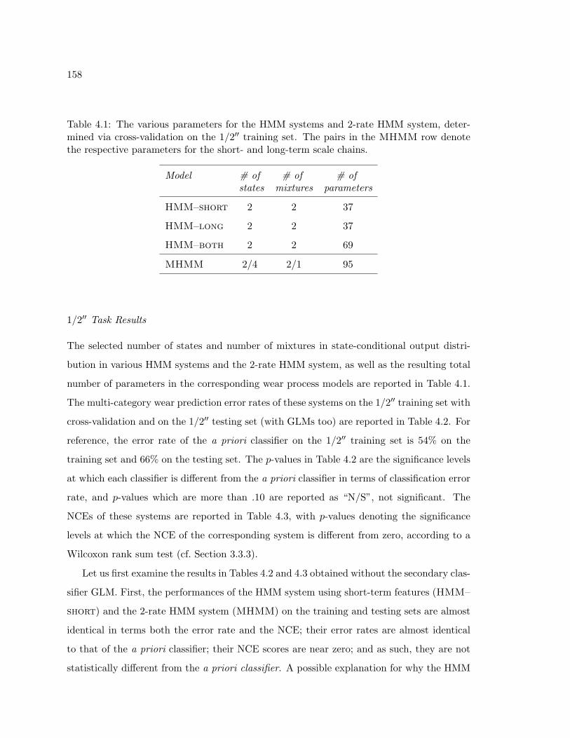
158
Table 4.1: The various parameters for the HMM systems and 2-rate HMM system, deter-mined via cross-validation on the 1/2′′ training set. The pairs in the MHMM row denotethe respective parameters for the short- and long-term scale chains.
Model # of # of # ofstates mixtures parameters
HMM–short 2 2 37
HMM–long 2 2 37
HMM–both 2 2 69
MHMM 2/4 2/1 95
1/2′′ Task Results
The selected number of states and number of mixtures in state-conditional output distri-
bution in various HMM systems and the 2-rate HMM system, as well as the resulting total
number of parameters in the corresponding wear process models are reported in Table 4.1.
The multi-category wear prediction error rates of these systems on the 1/2′′ training set with
cross-validation and on the 1/2′′ testing set (with GLMs too) are reported in Table 4.2. For
reference, the error rate of the a priori classifier on the 1/2′′ training set is 54% on the
training set and 66% on the testing set. The p-values in Table 4.2 are the significance levels
at which each classifier is different from the a priori classifier in terms of classification error
rate, and p-values which are more than .10 are reported as “N/S”, not significant. The
NCEs of these systems are reported in Table 4.3, with p-values denoting the significance
levels at which the NCE of the corresponding system is different from zero, according to a
Wilcoxon rank sum test (cf. Section 3.3.3).
Let us first examine the results in Tables 4.2 and 4.3 obtained without the secondary clas-
sifier GLM. First, the performances of the HMM system using short-term features (HMM–
short) and the 2-rate HMM system (MHMM) on the training and testing sets are almost
identical in terms both the error rate and the NCE; their error rates are almost identical
to that of the a priori classifier; their NCE scores are near zero; and as such, they are not
statistically different from the a priori classifier. A possible explanation for why the HMM

159
Table 4.2: The error rates and p-values for the statistical difference from the a prioriclassifier, for the HMM systems and the 2-rate HMM system on the 1/2′′ training set viacross-validation, and on the 1/2′′ testing set with and without the GLM posterior correction.
Model Training Set Testing Set Testing Setw/ GLM
error % p-value error % p-value error % p-value
HMM–short 64 N/S 62 N/S 43 2 · 10−3
HMM–long 8 10−9 43 2 · 10−3 43 2 · 10−3
HMM–both 8 10−9 45 5 · 10−3 43 2 · 10−3
HMM–both+ N/A N/A N/A N/A 45 5 · 10−3
MHMM 62 N/S 62 N/S 33 2 · 10−5
system using short-term features performs similar to the 2-rate HMM system is that the
most of the probability scores in the 2-rate HMM wear process models is due to the short-
term features, as each long-term feature corresponds to 40 short-term features. Second,
the performances of the HMM system using long-term features and the HMM system using
concatenated short- and long-term features are also identical in terms of both the error
rate and the NCE; they obtain excellent performance on the training set and statistically
different from the a priori classifier in terms of both criteria. A possible explanation for
why these two systems similarly perform is that in the concatenation system, the original
long-term features are oversampled by M (M = 40), highly skewing the resulting probabil-
ity scores towards that would be obtained using only the long-term features. Even though
their error rates on the testing set is relatively good and better than the a priori classifier,
but their NCE values on the testing set are negative and worse than that of the 2-rate HMM
system. (The testing set NCEs of the 2-rate HMM system and the HMM using long-term
features are statistically different at the level p = 0.11.) The fact that the feature concate-
nation approach receives a negative NCE score provides evidence for our hypothesis that
oversampling inherently long-term features introduces redundancy and gives bad confidence
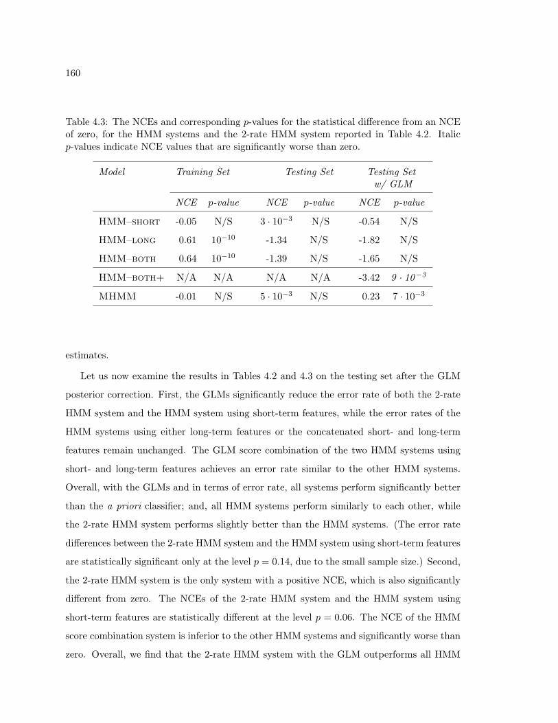
160
Table 4.3: The NCEs and corresponding p-values for the statistical difference from an NCEof zero, for the HMM systems and the 2-rate HMM system reported in Table 4.2. Italicp-values indicate NCE values that are significantly worse than zero.
Model Training Set Testing Set Testing Setw/ GLM
NCE p-value NCE p-value NCE p-value
HMM–short -0.05 N/S 3 · 10−3 N/S -0.54 N/S
HMM–long 0.61 10−10 -1.34 N/S -1.82 N/S
HMM–both 0.64 10−10 -1.39 N/S -1.65 N/S
HMM–both+ N/A N/A N/A N/A -3.42 9 · 10−3
MHMM -0.01 N/S 5 · 10−3 N/S 0.23 7 · 10−3
estimates.
Let us now examine the results in Tables 4.2 and 4.3 on the testing set after the GLM
posterior correction. First, the GLMs significantly reduce the error rate of both the 2-rate
HMM system and the HMM system using short-term features, while the error rates of the
HMM systems using either long-term features or the concatenated short- and long-term
features remain unchanged. The GLM score combination of the two HMM systems using
short- and long-term features achieves an error rate similar to the other HMM systems.
Overall, with the GLMs and in terms of error rate, all systems perform significantly better
than the a priori classifier; and, all HMM systems perform similarly to each other, while
the 2-rate HMM system performs slightly better than the HMM systems. (The error rate
differences between the 2-rate HMM system and the HMM system using short-term features
are statistically significant only at the level p = 0.14, due to the small sample size.) Second,
the 2-rate HMM system is the only system with a positive NCE, which is also significantly
different from zero. The NCEs of the 2-rate HMM system and the HMM system using
short-term features are statistically different at the level p = 0.06. The NCE of the HMM
score combination system is inferior to the other HMM systems and significantly worse than
zero. Overall, we find that the 2-rate HMM system with the GLM outperforms all HMM

161
Table 4.4: The various parameters for the HMM systems and 2-rate HMM system, deter-mined via cross-validation on the 1′′ data set. The pairs in the MHMM row denote therespective parameters for the short- and long-term scales.
Model # of # of # ofstates mixtures parameters
HMM–short 2 4 44
HMM–long 2 2 78
HMM–both 2 4 70
MHMM 2/1 2/1 67
systems in terms of both the error rate and NCE criteria, showing the utility of multi-rate
HMMs for multi-level tool-wear prediction. Either the feature concatenation or the classifier
combination approaches for combining different rate features in the HMM framework result
in negative NCE scores; the corresponding a posteriori prediction probabilities are not
reflective of the true wear level, confirming the hypothesis that redundancy reduction is
necessary for accurate confidence estimation.
1′′ Task Results
The 1′′ data set is relatively small, and it is only used in a cross-validation fashion (cf.
Section 3.3.6). The number of states and the number of mixtures per state-conditional
distribution for each system are again determined by choosing the pair resulting in lowest
error rate. These parameters as well as the total number of parameters in the resulting
wear process models are reported in Table 4.4. The multi-level wear prediction error rates
and the NCEs of the various HMM systems and the 2-rate HMM system are reported in
Table 4.5, where we also reported the statistical significance levels at which the error rates
are different from that of the a priori classifier and the NCEs are different from zero. For
reference, the error rate of the a priori classifier is 67%, which assigns all cutting passes in
the 1′′ data set to the most frequently occurring wear category in this data set.
The results on the 1′′ data set closely follow those on the 1/2′′ data set. First, the 2-rate

162
Table 4.5: The error rates and NCEs for the various HMM systems and the 2-rate HMMsystem on the 1′′ data set with cross-validation. Italic NCE p-values indicate significantlyworse than zero NCEs.
Model error % p-value NCE p-value(for error %) (for NCE)
HMM–short 44 0.01 -0.14 N/S
HMM–long 78 N/S -1.20 4 · 10−3
HMM–both 78 N/S -1.14 7 · 10−3
MHMM 48 0.04 -0.12 N/S
HMM system and the HMM system using short-term features perform similarly in terms
of both the error rate and the NCE criteria; and, their error rates are significantly better
than that of the a priori classifier, while their NCEs are not statistically different from
zero. Second, the HMM system using long-term features and the HMM system using the
concatenated short- and long-term features also perform similarly in terms of both criteria;
and, their error rates are similar to that of a priori classifier, while their NCEs are negative
and significantly worse than zero. These results are consistent with the results on the
1/2′′ data that the combination of short- and long-term information through the feature-
concatenated HMMs gives poor classification results and negative NCE values. Since the
1′′ data are only used in a cross-validation fashion, we cannot get an unbiased estimate of
performance using a GLM, and the observed superiority of the 2-rate HMM system over
the HMM systems with the GLMs on the 1/2′′ could not be confirmed.
Summary of Tool-Wear Monitoring Results
We can draw following conclusions from our experiments on the 1/2′′ and 1′′ tasks. First,
without the GLM posterior correction, the 2-rate HMM systems and the HMM systems
using short-term features perform similarly, but with the GLM posterior correction, the
2-rate HMM system significantly improves, especially in terms of NCE. Second, neither
the feature concatenation nor the score combination approaches in the HMM framework
163
are successful in integrating information in short- and long-term features, and they make
overconfident predictions with inferior NCE scores. This finding confirms our hypothesis
that reducing the redundancy of long-term observations is important for an unbiased es-
timate of the a posteriori classification probabilities. Overall, the 2-rate HMM performed
equally to or better than the HMM alternatives that we considered, in terms of both clas-
sification accuracy and confidence. Although error rates of the 2-rate HMM systems were
around 30 − 40%, the good results in NCE indicate that multi-rate HMMs can provide
useful outputs to human operators monitoring complex machining processes. In addition,
the parsimonious structure of the multi-rate HMMs allows for learning relatively complex
models from very sparse training data, which is particularly relevant to designing tool-wear
monitoring systems. Sparse data have been an important limitation of our experiments,
as well as other tool-wear research. It prevents exploring more sophisticated models that
might better represent complex wear processes, as they can quickly overfit when trained with
sparse data. In addition, sparse data have been problematic for reliable system comparison
to high certainty and for extracting diagnostics information.
Experimentation with different numbers of features (2−8), and feature reduction schemes
(such as linear discriminant analysis and principal component analysis), not reported, pro-
vided similar conclusions to those reported above.
4.3.2 Acoustic Modeling for Speech Recognition
The dominant acoustic modeling paradigm in speech recognition is based on phones and
short-time spectrum, where words are represented as sequences of phones, and phones are
characterized as three-state, left-to-right HMMs using cepstral features extracted every 10
msecs from 25 msec windows. Even though context-dependent phones and dynamic features
incorporate information from longer-time scales, the current HMM-based speech recogni-
tion systems focus on information and variability over less than 100 msecs. These systems
achieve impressive results on unconstrained conversational speech, for example, one of the
best performing systems in the NIST’s RT03 speech recognition benchmark had a 20.7%
WER [101], but their performances still lag an order of magnitude behind that of humans.
164
Many factors contribute to this relatively poor performance of speech recognition systems,
but the inaccuracy of current acoustic models to characterize variability associated with
conversational speech seems to be a large contributing factor, as demonstrated in a num-
ber of studies with real and simulated data. The study in [263] illustrates the effect of
speaking style on the speech recognition performance by comparing the recognition accu-
racy on spoken utterances to their transcribed and read versions. It is found that the WER
on the read versions is about the half of that on the spoken versions (28.8% vs. 52.6%).
A similar, more recent study [276] using speech from meetings had similar results: 36.7%
WER for read speech and 54.8% WER for spontaneous speech. The study in [187] conducts
experiments with simulated data to determine the effect of imperfect acoustic models on
recognition performance. Using hand-labeled phonetic transcriptions, they generate acous-
tic realizations for spoken utterances using an acoustic model which later also recognizes
the simulated speech. They found that the same acoustic model achieves 48.2% WER on
the real data and 41.3% WER on the simulated data. The absolute 7.9% WER reduction
in going from real to simulated data hints at the potential improvements solely due to more
accurate models in the existing speech recognition systems.
Our goal in this section is to improve the accuracy of current acoustic models by using
acoustic and linguistic information from longer time scales (up to 500 msecs) in addition
to the phonetic and short-term spectral information over less than 100 msecs. We will
use multi-rate HMMs to complement the usual sub-phonetic modeling units and short-time
spectral features with larger modeling units and long-term temporal features for a multi-
scale acoustic modeling of speech, as opposed to the pure short-time scale approach of the
current HMM-based acoustic models. We will explore two such multi-scale approaches using
2-rate HMM architectures with scales roughly corresponding to those of phones and sylla-
bles.3 In both applications, the fine scale in the 2-rate HMM acoustic models characterizes
acoustics using sub-phones and cepstral features similar to the current acoustic models.
They differ in the phenomena they characterize in the coarse scale. In the first application,
3A syllable is a unit of language, consisting of multiple phones. A syllable can be structured into threeordered parts: onset, nucleus, and coda, not all of which occur in every syllable. Onset and coda phonesare consonants, and nucleus phones are vowels.

165
we will use the coarse scale to broadly characterize phones using long-term TempoRAl Pat-
ternS (TRAPS) features (cf. Section 3.1.1) trained on phone targets, whereas in the second
application, the coarse scale characterizes a phenomenon different from phones, the lexi-
cal stress and syllable structure including broad consonant/vowel phone distinctions using
TRAPS trained on those targets. In the either application we aim to better characterize
the variability associated with conversation speech by using recognition units and informa-
tion from longer-time scales (up to 500 msecs) in addition to sub-phones and information
over less than 100 msecs. There is ample evidence from both human speech perception and
data-driven corpus studies that useful information lie in such longer time scales, which when
properly used in combination with short-term information, can improve speech recognition
accuracy.
Human speech perception shows sensitivity to slow changes on the spectrum, for ex-
ample the suppression of 2–8 Hz (corresponding to 125–500 msecs) modulation spectrum
significantly degrades speech intelligibility, whereas the suppression of those beyond 16 Hz
does not [91]. In addition, the human perceptual buffer can store up to 250 msecs, and it is
plausible that humans extract perceptual clues from such long time scales [130]. This claim
is also supported by the fact that many perceptual phenomena such as forward masking
and growth of loudness have time constants of several hundred of milliseconds [145]. In
addition to long-term acoustics, long-term contexts much wider than phones, especially syl-
lables, are important for speech recognition. Suprasegmental prosodic effects such as lexical
stress can significantly alter the acoustic realizations of phones. Lexical stress is important
for distinguishing between common confusion pairs such as seventeen vs. seventy, and
such stressed/unstressed syllable confusions are an important source of error for automatic
speech recognition systems. Pronunciation and durational variability observed in conversa-
tional speech also shows a high degree of dependence on the syllable structure [127, 129].
For example, phones occurring in syllable onsets are more likely to be preserved than those
on coda, which are more likely to substituted by another phone, or completely deleted.
The importance of long-term information and wide-context linguistic units have long
been recognized in speech recognition, and as mentioned earlier, the current HMM-based
acoustic models implicitly incorporate such long-term information via context-dependent

166
models, dynamic features, and feature normalization methods such as cepstral mean sub-
traction and RASTA [147]. Syllable features such as phone position in syllable and lexical
stress are relatively common for the clustering of context-dependent phones [246] and pro-
nunciation modeling [107]. Syllables have also proposed as a modeling unit alternative
to phones [114, 269]. The work in automatically derived acoustic modeling units such
as [17] showed that subword units bigger than phones are useful for acoustic modeling. In
speech signal processing, methods with long analysis windows such as modulation spectro-
gram [131] and TRAPS [148] have been proposed as an alternative to cepstral analysis. In
statistical modeling, modifications to HMMs, such as segment models [214], buried Markov
models [34], and auto-regressive HMMs [166] have been proposed for better representing
long-term dependencies in acoustic feature sequences. Various extensions of HMMs with
factored state and observation spaces such as coupled HMMs [52], mixed-memory Markov
models [242], and factorial HMMs [120] have been used in speech recognition for features
extracted from different frequency subbands and time scales [208, 209, 182].
Our approach to utilizing long-term acoustic information using multi-rate HMMs sig-
nificantly differs from but complimentary to some of the previous work in that multi-rate
HMMs combine acoustic cues from multiple time scales using both feature sequences and
modeling units. In particular, the speech is jointly modeled at multiple time scales with-
out introducing redundancy in long-term feature sequences by oversampling. As we have
demonstrated in our tool-wear monitoring experiments in Section 4.3.1, the advantages of
the redundancy reduction in the long-term feature sequences is two fold. Redundancy re-
duction in coarse features gives better confidence estimates, i.e. more accurate a posteriori
probabilities and better classification accuracy when they are integrated with another infor-
mation source (short-term features), as the evidence from coarser scales are not overcounted
as with oversampling. In this sense, the multi-rate statistical modeling framework explored
here is complimentary to the work exploring new signal processing methods, especially
those focusing on long-term information, as the HMMs might obscure gains from such new
features.
In the coming sections, we will present two applications of the 2-rate HMMs for joint
acoustic modeling of speech at two time scales, roughly corresponding to phones and syl-

167
lables. (Multi-scale acoustic modeling with more than two time scales is also possible with
multi-rate HMMs but not explored in this thesis due to higher computational cost, see
Section 7.2 for some possibilities.) For the short-time scale of our 2-rate HMM acoustic
models, we will use the traditional three-state phones and the cepstral features (PLPs)
extracted every 10 msec from 25 msec windows. For the long-time scale, we will explore
two approaches: the one where the long-time scale also represents phones but at a coarser
scale than three-state phones of the short-time scale, and the two where the long-time scale
represents the syllable structure and lexical stress in the spoken utterances. In each case,
we will use hidden activation TRAPS (HAT) features (cf. Section 3.1.1) trained on the
corresponding modeling units from 500 msec windows of speech as features. We will test
these two 2-rate HMM acoustic models and compare them with HMMs and alternative
methods of combining short- and long-term acoustic information on the nsh5 task, which is
described in Section 3.1.6. In our multi-rate models, we will also evaluate the variable-rate
extension described in Section 4.2.1 which we will use for focusing the analysis on transition
regions in the acoustic signal. Our speech recognition experiments aim to answer a number
of questions about the utility of multi-rate HMMs and long-term features and modeling
units for speech recognition:
1. Is the multi-rate approach to use long-term features better than the HMM- or coupled
HMM-based approaches that do not reduce redundancy in long-term features?
2. Is the explicit modeling of syllable structure, in particular syllable stress, helpful for
speech recognition?
3. Is the variable-rate sampling of long-term features to focus on fast-changing regions
more advantageous than the fixed-rate sampling schemes?
In the next section, we will first give baseline recognition results obtained with HMMs,
including the details of the n-best rescoring framework in GMTK that we use in our ex-
periments, and in the following sections, we will describe the two multi-rate HMM acoustic
models described above.
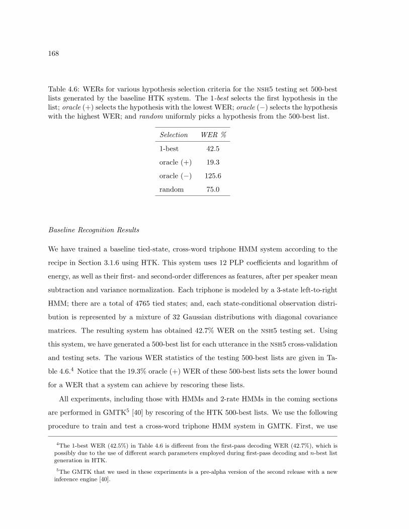
168
Table 4.6: WERs for various hypothesis selection criteria for the nsh5 testing set 500-bestlists generated by the baseline HTK system. The 1-best selects the first hypothesis in thelist; oracle (+) selects the hypothesis with the lowest WER; oracle (−) selects the hypothesiswith the highest WER; and random uniformly picks a hypothesis from the 500-best list.
Selection WER %
1-best 42.5
oracle (+) 19.3
oracle (−) 125.6
random 75.0
Baseline Recognition Results
We have trained a baseline tied-state, cross-word triphone HMM system according to the
recipe in Section 3.1.6 using HTK. This system uses 12 PLP coefficients and logarithm of
energy, as well as their first- and second-order differences as features, after per speaker mean
subtraction and variance normalization. Each triphone is modeled by a 3-state left-to-right
HMM; there are a total of 4765 tied states; and, each state-conditional observation distri-
bution is represented by a mixture of 32 Gaussian distributions with diagonal covariance
matrices. The resulting system has obtained 42.7% WER on the nsh5 testing set. Using
this system, we have generated a 500-best list for each utterance in the nsh5 cross-validation
and testing sets. The various WER statistics of the testing 500-best lists are given in Ta-
ble 4.6.4 Notice that the 19.3% oracle (+) WER of these 500-best lists sets the lower bound
for a WER that a system can achieve by rescoring these lists.
All experiments, including those with HMMs and 2-rate HMMs in the coming sections
are performed in GMTK5 [40] by rescoring of the HTK 500-best lists. We use the following
procedure to train and test a cross-word triphone HMM system in GMTK. First, we use
4The 1-best WER (42.5%) in Table 4.6 is different from the first-pass decoding WER (42.7%), which ispossibly due to the use of different search parameters employed during first-pass decoding and n-best listgeneration in HTK.
5The GMTK that we used in these experiments is a pre-alpha version of the second release with a newinference engine [40].
169
HTK to induce state-tying clusters and estimate a single mixture Gaussian output distri-
bution for each tied state, which are then transferred to GMTK to initialize the tied-state
parameters in GMTK. Starting from these single-mixture output distributions and clustered
states, we apply a mixture splitting regime in GMTK until the desired number of mixture
components in state-conditional observation distributions is achieved. Between each split,
three iterations of the EM algorithm is applied. If at any point during training a mixture
component receives a weight that is less than 120·M , M denoting the number of mixtures in
the mixture, then it vanishes. After the desired number of mixtures is achieved, we continue
EM training until the relative increase in the log-likelihood is less than 0.2%. To reduce the
computational cost of training, only a single pronunciation for each word in the training
transcriptions is considered, which are obtained by a forced-alignment using the HTK sys-
tem that was used to generate the 500-best lists. We will use these pronunciation-aligned
training transcripts in all remaining experiments in GMTK.
The n-best list rescoring in GMTK is performed by finding the acoustic log-likelihood
score of each hypothesis in the n-best list, then adding these scores to the corresponding
language modeling scores. Given an n-best list, the hypothesis with the highest combined
score is chosen as the recognition hypothesis. Similar to the use of phone sequences instead
of word sequences in our training, the acoustic score of an utterance is calculated using
the Viterbi-aligned phone sequence obtained by the baseline HTK system.6 As in first-
pass decoding, we use language model scaling factors and insertion penalties to modify
the original language modeling scores, which are tuned on the cross-validation set over a
range of scaling factors and insertion penalties. The GMTK equivalent of the baseline HTK
system in GMTK has obtained 42.3% WER on the nsh5 testing set, which is better than
42.7% WER of the HTK system with first-pass decoding. For comparison, rescoring of the
500-best lists using the HTK system, as opposed to first-pass decoding, results in a 42.7%
WER, the same as that in the first-pass decoding with HTK.
6When computing acoustic likelihood scores over word sequences, multiple pronunciations of each wordas well as optional silences between words contribute to the total likelihood score. On the other hand, inthe likelihood computation over the force-aligned phone sequences, a single pronunciation for each word isused, and the presence or absence of inter-word silences are a priori determined during force-alignments.However, we found that the likelihoods obtained by two scoring methods in our experiments are almostidentical and differ by about 0.001%, relatively.
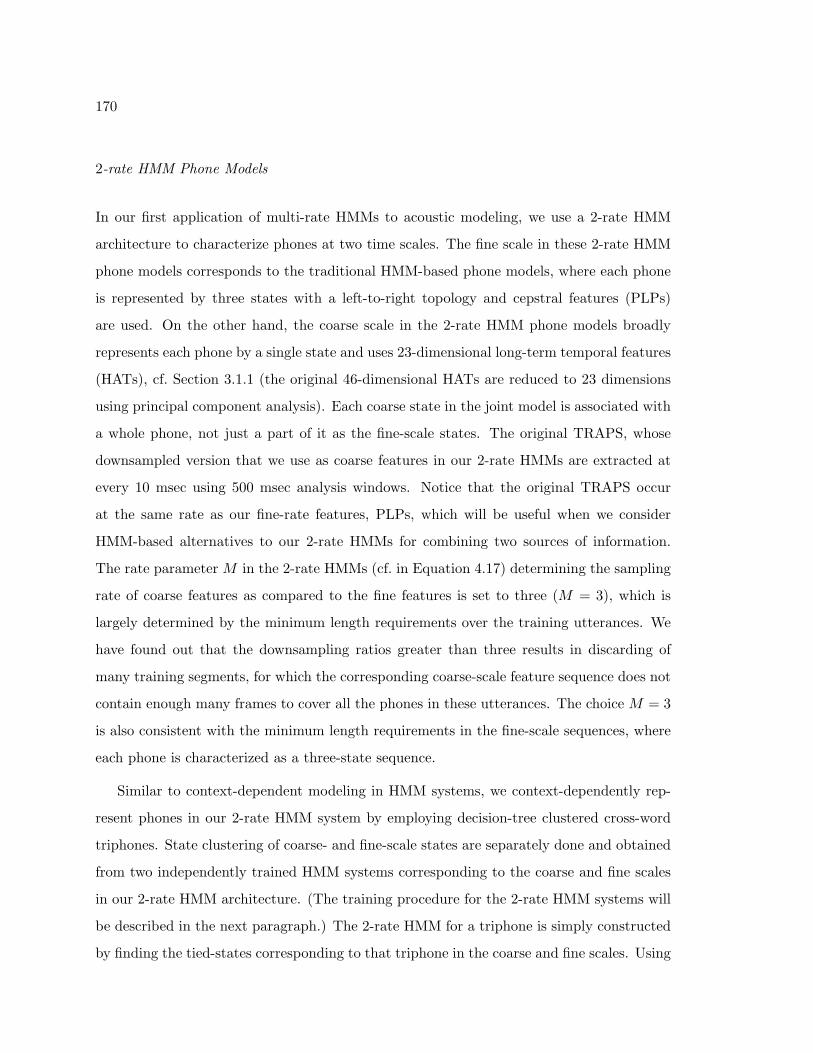
170
2-rate HMM Phone Models
In our first application of multi-rate HMMs to acoustic modeling, we use a 2-rate HMM
architecture to characterize phones at two time scales. The fine scale in these 2-rate HMM
phone models corresponds to the traditional HMM-based phone models, where each phone
is represented by three states with a left-to-right topology and cepstral features (PLPs)
are used. On the other hand, the coarse scale in the 2-rate HMM phone models broadly
represents each phone by a single state and uses 23-dimensional long-term temporal features
(HATs), cf. Section 3.1.1 (the original 46-dimensional HATs are reduced to 23 dimensions
using principal component analysis). Each coarse state in the joint model is associated with
a whole phone, not just a part of it as the fine-scale states. The original TRAPS, whose
downsampled version that we use as coarse features in our 2-rate HMMs are extracted at
every 10 msec using 500 msec analysis windows. Notice that the original TRAPS occur
at the same rate as our fine-rate features, PLPs, which will be useful when we consider
HMM-based alternatives to our 2-rate HMMs for combining two sources of information.
The rate parameter M in the 2-rate HMMs (cf. in Equation 4.17) determining the sampling
rate of coarse features as compared to the fine features is set to three (M = 3), which is
largely determined by the minimum length requirements over the training utterances. We
have found out that the downsampling ratios greater than three results in discarding of
many training segments, for which the corresponding coarse-scale feature sequence does not
contain enough many frames to cover all the phones in these utterances. The choice M = 3
is also consistent with the minimum length requirements in the fine-scale sequences, where
each phone is characterized as a three-state sequence.
Similar to context-dependent modeling in HMM systems, we context-dependently rep-
resent phones in our 2-rate HMM system by employing decision-tree clustered cross-word
triphones. State clustering of coarse- and fine-scale states are separately done and obtained
from two independently trained HMM systems corresponding to the coarse and fine scales
in our 2-rate HMM architecture. (The training procedure for the 2-rate HMM systems will
be described in the next paragraph.) The 2-rate HMM for a triphone is simply constructed
by finding the tied-states corresponding to that triphone in the coarse and fine scales. Using
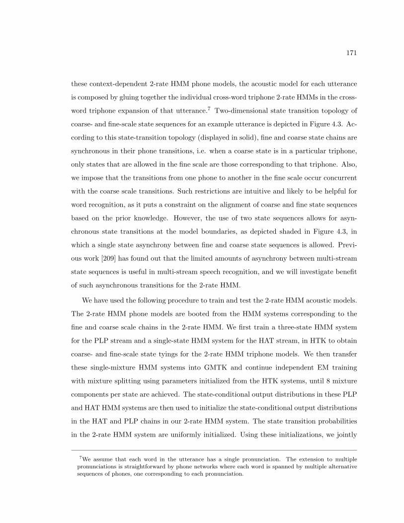
171
these context-dependent 2-rate HMM phone models, the acoustic model for each utterance
is composed by gluing together the individual cross-word triphone 2-rate HMMs in the cross-
word triphone expansion of that utterance.7 Two-dimensional state transition topology of
coarse- and fine-scale state sequences for an example utterance is depicted in Figure 4.3. Ac-
cording to this state-transition topology (displayed in solid), fine and coarse state chains are
synchronous in their phone transitions, i.e. when a coarse state is in a particular triphone,
only states that are allowed in the fine scale are those corresponding to that triphone. Also,
we impose that the transitions from one phone to another in the fine scale occur concurrent
with the coarse scale transitions. Such restrictions are intuitive and likely to be helpful for
word recognition, as it puts a constraint on the alignment of coarse and fine state sequences
based on the prior knowledge. However, the use of two state sequences allows for asyn-
chronous state transitions at the model boundaries, as depicted shaded in Figure 4.3, in
which a single state asynchrony between fine and coarse state sequences is allowed. Previ-
ous work [209] has found out that the limited amounts of asynchrony between multi-stream
state sequences is useful in multi-stream speech recognition, and we will investigate benefit
of such asynchronous transitions for the 2-rate HMM.
We have used the following procedure to train and test the 2-rate HMM acoustic models.
The 2-rate HMM phone models are booted from the HMM systems corresponding to the
fine and coarse scale chains in the 2-rate HMM. We first train a three-state HMM system
for the PLP stream and a single-state HMM system for the HAT stream, in HTK to obtain
coarse- and fine-scale state tyings for the 2-rate HMM triphone models. We then transfer
these single-mixture HMM systems into GMTK and continue independent EM training
with mixture splitting using parameters initialized from the HTK systems, until 8 mixture
components per state are achieved. The state-conditional output distributions in these PLP
and HAT HMM systems are then used to initialize the state-conditional output distributions
in the HAT and PLP chains in our 2-rate HMM system. The state transition probabilities
in the 2-rate HMM system are uniformly initialized. Using these initializations, we jointly
7We assume that each word in the utterance has a single pronunciation. The extension to multiplepronunciations is straightforward by phone networks where each word is spanned by multiple alternativesequences of phones, one corresponding to each pronunciation.
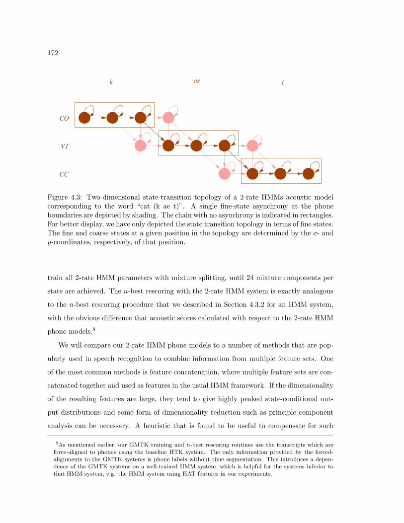
172
������������������������������
������������������������������
������������������������������
������������������������������
������������������������������
������������������������������
������������������������������
������������������������������
������������
������������
������������������������������
������������������������������
� � � � � � � � � � � �
������������������������������
������������������������������
������������������������������
������������������������������
������������������������������
������������������������������
������������������������������
������������������������������
������������������������������
������������������������������
������������������������������
������������������������������
������������������������������
���������������������������������������������������������������������������������������������������
���������������������������������������������������������������������������������������������������
���������������������������������������������������������������������������������
���������������������������������������������������������������������������������
CO
CC
V1
k ae t
Figure 4.3: Two-dimensional state-transition topology of a 2-rate HMMs acoustic modelcorresponding to the word “cat (k ae t)”. A single fine-state asynchrony at the phoneboundaries are depicted by shading. The chain with no asynchrony is indicated in rectangles.For better display, we have only depicted the state transition topology in terms of fine states.The fine and coarse states at a given position in the topology are determined by the x- andy-coordinates, respectively, of that position.
train all 2-rate HMM parameters with mixture splitting, until 24 mixture components per
state are achieved. The n-best rescoring with the 2-rate HMM system is exactly analogous
to the n-best rescoring procedure that we described in Section 4.3.2 for an HMM system,
with the obvious difference that acoustic scores calculated with respect to the 2-rate HMM
phone models.8
We will compare our 2-rate HMM phone models to a number of methods that are pop-
ularly used in speech recognition to combine information from multiple feature sets. One
of the most common methods is feature concatenation, where multiple feature sets are con-
catenated together and used as features in the usual HMM framework. If the dimensionality
of the resulting features are large, they tend to give highly peaked state-conditional out-
put distributions and some form of dimensionality reduction such as principle component
analysis can be necessary. A heuristic that is found to be useful to compensate for such
8As mentioned earlier, our GMTK training and n-best rescoring routines use the transcripts which areforce-aligned to phones using the baseline HTK system. The only information provided by the forced-alignments to the GMTK systems is phone labels without time segmentation. This introduces a depen-dence of the GMTK systems on a well-trained HMM system, which is helpful for the systems inferior tothat HMM system, e.g. the HMM system using HAT features in our experiments.
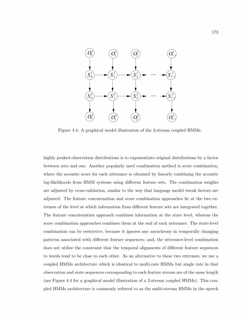
173
S 0 S S2 2 2
O20O O12 2 2
1 2... 2
OT−12
S T−1
S 0 S S1 2... S T−1
O20O O1 OT−1
1 1 1 1
1 1 1 1
Figure 4.4: A graphical model illustration of the 2-stream coupled HMMs.
highly peaked observation distributions is to exponentiate original distributions by a factor
between zero and one. Another popularly used combination method is score combination,
where the acoustic score for each utterance is obtained by linearly combining the acoustic
log-likelihoods from HMM systems using different feature sets. The combination weights
are adjusted by cross-validation, similar to the way that language model tweak factors are
adjusted. The feature concatenation and score combination approaches lie at the two ex-
tremes of the level at which information from different feature sets are integrated together.
The feature concatenation approach combines information at the state level, whereas the
score combination approaches combines them at the end of each utterance. The state-level
combination can be restrictive, because it ignores any asynchrony in temporally changing
patterns associated with different feature sequences; and, the utterance-level combination
does not utilize the constraint that the temporal alignments of different feature sequences
to words tend to be close to each other. As an alternative to these two extremes, we use a
coupled HMMs architecture which is identical to multi-rate HMMs but single rate in that
observation and state sequences corresponding to each feature stream are of the same length
(see Figure 4.4 for a graphical model illustration of a 2-stream coupled HMMs). This cou-
pled HMMs architecture is commonly referred to as the multi-stream HMMs in the speech

174
recognition literature [47, 48]. Both multi-rate HMMs and multi-stream HMMs synchronize
modeling units in each feature stream at some temporal anchor points, such as phone bound-
aries, and as such, they lie between state- and utterance-level combination extremes. In our
experimental set up, the only difference of our 2-stream HMM system from our 2-rate HMM
system is that the multi-stream models use oversampled HAT feature sequences that are of
the same rate as the PLP feature sequences. Thus, the performance comparisons between
the 2-stream HMM system and the 2-rate HMM system test the hypothesis that whether
or not redundancy reduction in the coarse feature sequences is useful for recognition.
We will also compare 2-rate HMM acoustic models described above which uses a fixed-
rate sampling scheme for coarse features to a variable-rate sampling scheme based on the
extension in Section 4.2.1. The optimality of a fixed-rate downsampling scheme for speech
recognition is questionable, because phones in English show a high-degree of durational
variability depending on both phonetic context (e.g., 10–30 msecs for stop consonants 100–
150 msecs for vowels) and speaking rate. A time-invariant downsampling might fall short
of resolving phones with very short duration. In addition, from an information extraction
perspective, the variable-rate sampling might also be more desirable, as it can tailor the
signal analysis to focus more on information-bearing regions, such as phone transitions in
speech recognition, as opposed to giving uniform emphasis over the signal space including
long silences and vowel centers which are relatively easy to recognize due to their long
duration. In contrast, a variable-rate sampling scheme can dynamically adjust the modeling
resolution at the coarse scale with respect to changing signal characteristics. Thus, we have
also trained and tested a 2-rate HMM system that is identical to the 2-rate HMM system
described above but uses a variable-rate sampling method for the coarse features (HATs).
The procedure for time-varying sampling of coarse features involves automatically picking
feature vectors only when they significantly differ from the ones occurring before, where
differences are computed in terms of the squared error [6]. We applied such a frame picking
algorithm to the PLP sequence for each utterance to obtain a partitioning of PLP vectors
into contiguous blocks (which, on average, consists of three frames), and for each block
the corresponding feature in the HAT feature stream is sampled. The 2-rate HMM system
using variable-rate sampling is identical to the 2-rate HMM system, and we used the same
175
training and testing procedures. The concept of state asynchrony at the phone transitions
also apply to the variable-rate extensions and will be evaluated.
The performances of the 2-rate HMM system with various degree of state asynchrony
and other related systems on the nsh5 testing set are presented in Table 4.7. Recognition
results are obtained by rescoring of the 500-best lists generated by the baseline HTK system
(cf. Section 4.3.2). All systems in this table are trained and tested in GMTK; the HMM
system using PLPs have 32 mixture components in its output distributions; and, the total
number of parameters in other systems except the HMM systems using HATs is roughly
made equal to each other by adjusting the mixture components at their state-conditional
output distributions. The same training procedure as the procedure for training the 2-rate
HMM systems with fixed-rate sampling is used to train the 2-stream HMM systems and the
2-rate HMM systems with variable-rate sampling. The concept of state asynchrony at the
phone boundaries also apply to the 2-stream HMMs, and we report results with 2-stream
HMM systems which do and do not allow one fine-scale (PLP stream) state asynchrony at
the phone boundaries.
We make the following observations based on the results presented in Table 4.7. First,
we note that HATs features by themselves in the HMM framework are inferior to the PLP
features, but they do contain complimentary information, as exemplified by the fact that
they always improve recognition accuracy when combined with PLPs, regardless of the
combination method. Also, the three HMM systems using HAT features with (fixed- or
variable-rate) and without downsampling perform surprisingly well, considering the fact
that they represent each phone by a single state, but this is mainly an artifact of the n-best
rescoring test paradigm. The total number of clustered states in the HMM system using
original HATs is more than twice that of the HMM system using downsampled by 3 HATs,
which is due to the fact that the former system has almost three times as much training data.
We also find that the HMM system using variable-rate downsampled HATs outperforms
the HMM system using fixed-rate downsampled HATs, confirming our hypothesis that it is
advantageous to focus on more information-bearing regions (which are the transition regions
in speech) rather than a uniform emphasis over the signal space. Second, we observe that
the state-level combination of PLPs and HATs via feature concatenation clearly outperforms
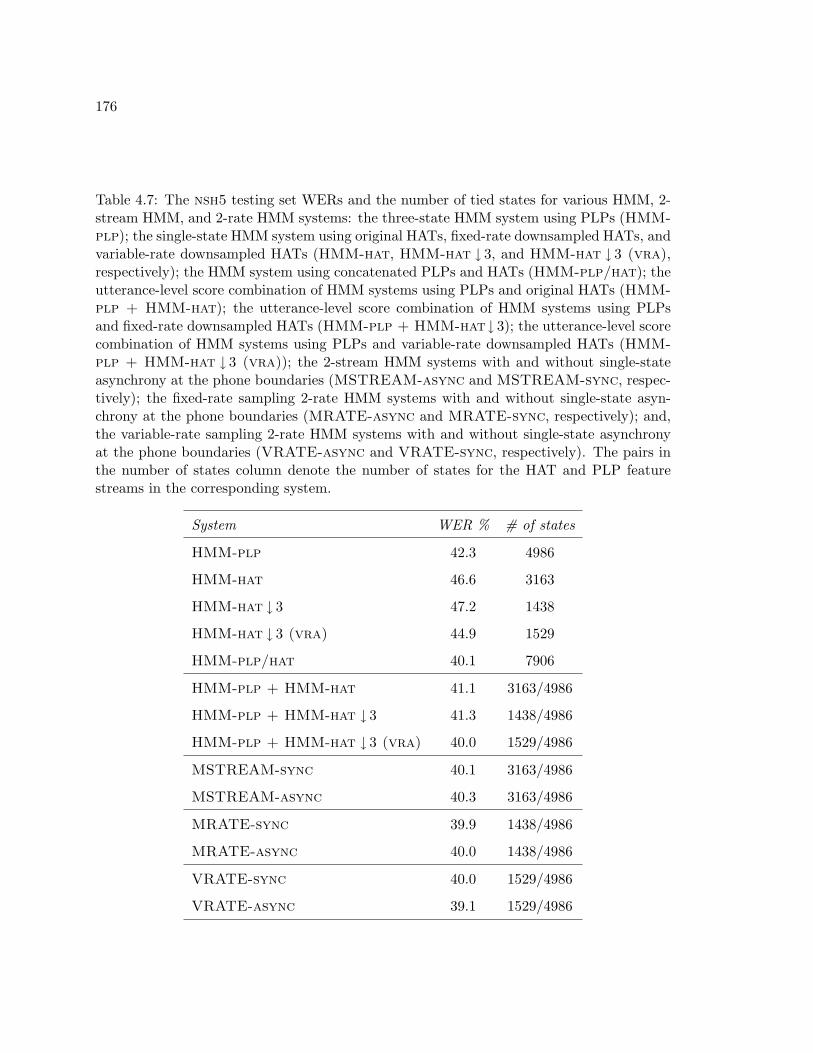
176
Table 4.7: The nsh5 testing set WERs and the number of tied states for various HMM, 2-stream HMM, and 2-rate HMM systems: the three-state HMM system using PLPs (HMM-plp); the single-state HMM system using original HATs, fixed-rate downsampled HATs, andvariable-rate downsampled HATs (HMM-hat, HMM-hat ↓ 3, and HMM-hat ↓ 3 (vra),respectively); the HMM system using concatenated PLPs and HATs (HMM-plp/hat); theutterance-level score combination of HMM systems using PLPs and original HATs (HMM-plp + HMM-hat); the utterance-level score combination of HMM systems using PLPsand fixed-rate downsampled HATs (HMM-plp + HMM-hat↓ 3); the utterance-level scorecombination of HMM systems using PLPs and variable-rate downsampled HATs (HMM-plp + HMM-hat ↓ 3 (vra)); the 2-stream HMM systems with and without single-stateasynchrony at the phone boundaries (MSTREAM-async and MSTREAM-sync, respec-tively); the fixed-rate sampling 2-rate HMM systems with and without single-state asyn-chrony at the phone boundaries (MRATE-async and MRATE-sync, respectively); and,the variable-rate sampling 2-rate HMM systems with and without single-state asynchronyat the phone boundaries (VRATE-async and VRATE-sync, respectively). The pairs inthe number of states column denote the number of states for the HAT and PLP featurestreams in the corresponding system.
System WER % # of states
HMM-plp 42.3 4986
HMM-hat 46.6 3163
HMM-hat ↓ 3 47.2 1438
HMM-hat ↓ 3 (vra) 44.9 1529
HMM-plp/hat 40.1 7906
HMM-plp + HMM-hat 41.1 3163/4986
HMM-plp + HMM-hat ↓ 3 41.3 1438/4986
HMM-plp + HMM-hat ↓ 3 (vra) 40.0 1529/4986
MSTREAM-sync 40.1 3163/4986
MSTREAM-async 40.3 3163/4986
MRATE-sync 39.9 1438/4986
MRATE-async 40.0 1438/4986
VRATE-sync 40.0 1529/4986
VRATE-async 39.1 1529/4986

177
the utterance-level score combination approaches (in the cases with original HATs and the
fixed-rate downsampled HATs), showing the importance of integrating different information
sources at an early stage. In addition, the feature concatenation of PLPs and HATs gives
a significant improvement over the HMM system using PLPs. Third, the performances of
the HMM system with concatenated features and the 2-rate and 2-stream HMM systems
without asynchrony are similar to each other, while the 2-rate HMM system being slightly
better (though the improvement is not statistically significant). However, the 2-rate HMM
systems are computationally more efficient when decoding, as they involve fewer Gaussian
computations due to the fact that they involve fewer number of tied states and feature
vectors in the HAT stream. The state asynchrony at the phone boundaries does not help
and even slightly decreases performance in both the 2-rate HMM with fixed-rate system and
2-stream HMM systems. Fourth, the variable-rate sampling extension of multi-rate HMMs
clearly outperforms all other systems when used with asynchrony. This finding provides
evidence towards our hypotheses that reducing the redundancy of long-term features is
necessary when combining different information sources, and that tailoring the analysis on
more information regions (which are the transition regions in speech) could be helpful in
pattern recognition.
Our results show that downsampled HATs contain as much information as the original
HATs about the broadly modeled phones, and a multi-rate modeling approach for combining
information in HATs with that in PLPs is advantageous, in terms of both accuracy and
computational efficiency, to approaches that do not reduce their redundancy. Overall, we
find an advantage to match the scale of features to the modeling units, which is long-term
HATs to broad phones in the experiments above. The latter claim also implies that the
2-stream HMM architecture might be more appropriate when the coarse feature stream
represents some phenomenon which is of the same scale as the oversampled HAT features.
To test this hypothesis, we have trained and tested a new 2-stream HMM system, which
uses three-state phones in the HAT stream, as opposed to using single-state phones in the
HAT stream as in the 2-stream HMM systems in Table 4.7 (the PLP stream still represents
three state phones). This new 2-stream HMM system with the increased temporal detail
in HAT stream gave a 39.7% WER, which is better than the 40.1% WER of the 2-stream
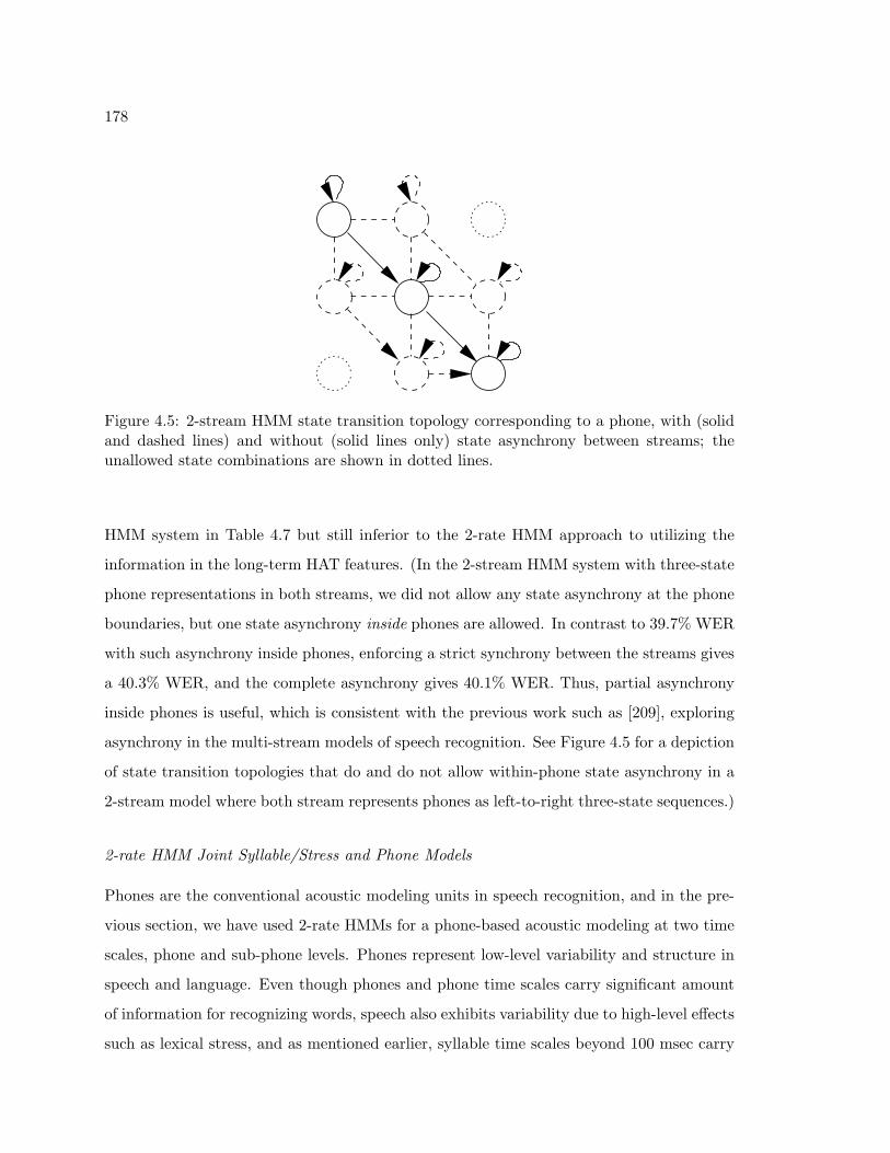
178
Figure 4.5: 2-stream HMM state transition topology corresponding to a phone, with (solidand dashed lines) and without (solid lines only) state asynchrony between streams; theunallowed state combinations are shown in dotted lines.
HMM system in Table 4.7 but still inferior to the 2-rate HMM approach to utilizing the
information in the long-term HAT features. (In the 2-stream HMM system with three-state
phone representations in both streams, we did not allow any state asynchrony at the phone
boundaries, but one state asynchrony inside phones are allowed. In contrast to 39.7% WER
with such asynchrony inside phones, enforcing a strict synchrony between the streams gives
a 40.3% WER, and the complete asynchrony gives 40.1% WER. Thus, partial asynchrony
inside phones is useful, which is consistent with the previous work such as [209], exploring
asynchrony in the multi-stream models of speech recognition. See Figure 4.5 for a depiction
of state transition topologies that do and do not allow within-phone state asynchrony in a
2-stream model where both stream represents phones as left-to-right three-state sequences.)
2-rate HMM Joint Syllable/Stress and Phone Models
Phones are the conventional acoustic modeling units in speech recognition, and in the pre-
vious section, we have used 2-rate HMMs for a phone-based acoustic modeling at two time
scales, phone and sub-phone levels. Phones represent low-level variability and structure in
speech and language. Even though phones and phone time scales carry significant amount
of information for recognizing words, speech also exhibits variability due to high-level effects
such as lexical stress, and as mentioned earlier, syllable time scales beyond 100 msec carry

179
important information for speech recognition. Incorporating such acoustic features and/or
modeling units from syllable time scales might help to explain some of the variability in
the phone time scale and resolve some of the confusions that cannot be resolved based on
short-term information alone.
Our goal in this section is to jointly model speech at both phone and syllable time scales
using associated modeling units and feature sequences in a 2-rate HMM architecture. The
fine scale of the proposed 2-rate HMM acoustic models again corresponds to the traditional
short-term representation of speech using sub-phones and cepstral features. The innova-
tive part of the proposed architecture lies in its coarse scale, representing syllable structure
(onset, nucleus, and coda), and lexical stress. In particular, the coarse scale models gen-
eral consonant/vowel phone classes but differentiates between onset, coda, and ambisyllabic
consonants, and between stressed and unstressed vowels. Motivations for characterizing
syllable structure and lexical stress in the proposed models mainly come from statistical
analysis of conversational speech corpora and errors made by HMM speech recognizers.
First, analyses in [128] on subsets of Switchboard (conversational speech) and TIMIT (read
speech) corpora, both of which are hand-transcribed at phone and syllable levels, showed
that actually spoken version of words exhibit systematic variations from their canonical pro-
nunciations with respect to syllable structure: syllable onsets are mostly preserved in read
or conversational speech (85−91%), but the codas are less often preserved in conversational
speech (63%) than in read speech (81%); and, codas are more subject to complete substitu-
tions or deletions than onsets. Similar syllable-dependent systematic variations have been
found for durational variability of phones in [128]. Second, in [268] it is illustrated that
the knowledge of timing of syllable onsets can significantly reduce WER (38% in an oracle
experiment in the Numbers ’95 task), and as such, explicit modeling of syllable onsets could
be helpful. Third, anecdotally, stressed and unstressed syllable confusions in word pairs
such as seventeen and seventy are a common source of error for both humans and speech
recognition systems. For example, such word pairs are responsible for a large portion of
errors made by a phone-based HMM speech recognizer on the Numbers ’95 task [98]. More
quantitatively, we analyzed the stress errors made by our baseline HMM system using PLP
features (HMM-plp in Table 4.7). We first forced-aligned recognition outputs and reference

180
transcripts into phones using a stress-marked dictionary. We then mapped these aligned
phones into five classes: consonants, stressed and unstressed vowels, silence, and non-speech.
In terms of these five broad classes, the system has 18.3% token error rate, of which 3.3%,
10.4%, and 5.1% are substitution, deletion, and insertion, respectively, errors. Deletions
are the dominant error type, of which 49% are due to consonants, and 34% are due to the
stressed vowels. A significant reduction in such stress confusions by an explicit modeling of
stress might also transfer into avoiding some word confusions. Based on the findings of these
studies phones, we expect that explicit modeling onset, coda, and ambisyllabic consonants
as well as stressed and unstressed vowels could improve speech recognition accuracy.
As mentioned before, the fine scale in the proposed 2-rate HMM joint syllable/stress
and phone models represents each phone as a three state left-to-right sequence and uses
short-time cepstrum (PLP) as features. On the other hand, the coarse scale in these models
involves: (1) acoustic units corresponding to onset, coda, and ambisyllabic consonants;
stressed and unstressed vowels; and, two additional classes for silence and non-speech sounds
such as noise; and (2) acoustic features (HATs) which are trained to predict to these seven
classes of sounds. (Since the HATs are trained to predict these seven classes, they are 7-
dimensional, but we also used their first- and second order differences as features to make
them comparable to the 23-dimensional HAT features of the phone modeling experiments
in Section 4.3.2.) In our 2-rate HMM speech recognition system, each 2-rate HMM unit
corresponds to a syllable part (onset, coda, and nucleus). The single coarse state in such a
2-rate HMM unit indicates one of the seven broad classes, whereas the fine state sequence for
that unit is obtained by concatenating the state sequences of the phones in that syllable part.
The models for words are composed by gluing together 2-rate HMM units corresponding to
syllable constituents in that word. For example. the 2-rate HMM sequence corresponding
to the word seventeen is constructed as follows. We first use a stress and syllable marked
dictionary9 to decompose words into its constituting phones and syllables as follows:
seventeen [ s + eh [ v ] . ax n ] [ t + iy n ]
9The dictionary and syllable coding used in this dictionary is first developed in [215], and later modifiedby [246]. For our work, we modified the dictionary of [246] for a slightly different phone set and addednew words.
181
where the phone sequence between an open bracket and a close one corresponds to a syllable,
and ’+’ and ’.’ are stress and no-stress markers respectively, for vowels. In the syllable
[t iy n], t is the onset, iy is the nucleus, and n is the coda. The phone v is ambisyllabic,
as it is both the coda of first syllable [s eh v] and the onset of second syllable [v ax n].
Using this syllable and phone pronunciation of the word seventeen, the coarse and fine
state sequences in the composite model of this word is given as follows:
| CO | V1 | CA | V0 | CC | CO | V1 | CC |
|s(1-2-3)|eh(1-2-3)|v(1-2-3)|ax(1-2-3)|n(1-2-3)|t(1-2-3)|iy(1-2-3)|n(1-2-3)|
where | denotes a 2-rate HMM boundary; CO, CC, and CA denote onset, coda, and ambi-
syllabic, respectively, consonants; V0, and V1 denote unstressed and stressed, respectively,
vowels; and x(1-2-3) denotes the 3-state sequence corresponding to the phone x. For
simplicity, we have used context-independent states in the above display, but in our imple-
mentation, we use left and right context-dependent states at both scales. The concept of
state asynchrony at the phone boundaries that we explored in the context of 2-rate HMM
phone models applies equally well to our joint syllable/stress and phone models but at the
syllable constituent boundaries. The same training and testing procedures as those for the
2-rate HMM phone system described in Section 4.3.2 are used except the difference that ini-
tializing HMM for the coarse scale of the 2-rate HMM joint syllable/stress and phone models
uses our seven broad phone classes (CO, CC, CA, V0, V1, sil, noise) as its modeling
units instead of phones and a pronouncing dictionary consisting of these labels. We again
set the downsampling ratio of coarse features to three due to the minimum length require-
ments. We have also explored the benefit of variable-rate extension of 2-rate HMMs for
the present 2-rate joint syllable/stress and phone models using the same sampling scheme
described in Section 4.3.2.
We have trained and tested 2-rate HMM joint syllable/stress and phone systems with
fixed- and variable-rate sampling schemes as well as with and without state asynchrony at
the phone boundaries on the nsh5 task. As alternatives to the multi-rate HMM framework,
feature concatenation and utterance-level score combination approaches to combining short-
and long-term information in the HMM framework are also tested. Continuing with our

182
comparisons between multi-rate and multi-stream HMMs, a 2-stream HMM system, which
is identical to the described 2-rate HMMs system but uses original HATs features without
downsampling is trained. The performances of the 2-rate HMM systems and various HMM
and 2-stream HMM systems on the nsh5 testing set are presented Table 4.8. All systems in
this table are trained and tested in GMTK using the procedures described in Section 4.3.2;
the baseline HMM system using PLPs in Table 4.8 is the same as the one in Table 4.7;
and, all systems except the two HMM systems using HATs have roughly equal number of
parameters. These two HMM systems use the seven broad phone classes as their acoustic
modeling units, instead of phones as in other HMM systems.
We make the following observations based on the results presented in Table 4.8. First,
the number of parameters associated with the HMM system using HATs and seven broad
classes as recognition units is very small, and as such, the additional parameter complexity
of the various joint syllable/stress and phone models over the baseline HMM phone models
is very small (less than 2%, relatively). This is not surprising given that there are only 343
possible context-dependent unit combinations for 7 broad phone classes, some of which are
linguistically impossible. Yet, the performance of the HMM systems using HATs and those
broad classes as recognition units is surprisingly good, which is again an artifact of the
n-best rescoring paradigm. We also find a slight advantage to using the variable-rate down-
sampled HATs as compared to using the fixed-rate downsampled HATs but the difference
is not as pronounced as that in Table 4.7. Second, we find that neither feature concatena-
tion nor score combination approaches to combining information in PLPs and HATs in the
HMM framework is successful, and in fact, performance degrades significantly in the former
approach. We note that this is unlike similar experiments we performed in Section 4.3.2
(cf. Table 4.7) using HATs trained on phone targets. Third, we note that the new HAT
features, when used in 2-stream HMMs, only give a slight improvement over the baseline
HMM system using PLPs; and, the state asynchrony at the phone transition boundaries
is clearly hurtful for the 2-stream HMM models. Overall, neither the HMM-based feature
concatenation and score combination approaches nor the 2-stream approach seems to make
use of the complimentary information in HATs. Fourth, in contrast, the 2-rate HMM sys-
tem gives a significant improvement over the baseline HMM system using PLPs, and the
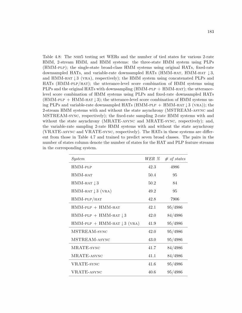
183
Table 4.8: The nsh5 testing set WERs and the number of tied states for various 2-rateHMM, 2-stream HMM, and HMM systems: the three-state HMM system using PLPs(HMM-plp); the single-state broad-class HMM systems using original HATs, fixed-ratedownsampled HATs, and variable-rate downsampled HATs (HMM-hat, HMM-hat ↓ 3,and HMM-hat ↓ 3 (vra), respectively); the HMM system using concatenated PLPs andHATs (HMM-plp/hat); the utterance-level score combination of HMM systems usingPLPs and the original HATs with downsampling (HMM-plp + HMM-hat); the utterance-level score combination of HMM systems using PLPs and fixed-rate downsampled HATs(HMM-plp + HMM-hat ↓ 3); the utterance-level score combination of HMM systems us-ing PLPs and variable-rate downsampled HATs (HMM-plp + HMM-hat ↓ 3 (vra)); the2-stream HMM systems with and without the state asynchrony (MSTREAM-async andMSTREAM-sync, respectively); the fixed-rate sampling 2-rate HMM systems with andwithout the state asynchrony (MRATE-async and MRATE-sync, respectively); and,the variable-rate sampling 2-rate HMM systems with and without the state asynchrony(VRATE-async and VRATE-sync, respectively). The HATs in these systems are differ-ent from those in Table 4.7 and trained to predict seven broad classes. The pairs in thenumber of states column denote the number of states for the HAT and PLP feature streamsin the corresponding system.
System WER % # of states
HMM-plp 42.3 4986
HMM-hat 50.4 95
HMM-hat ↓ 3 50.2 84
HMM-hat ↓ 3 (vra) 49.2 95
HMM-plp/hat 42.8 7906
HMM-plp + HMM-hat 42.1 95/4986
HMM-plp + HMM-hat ↓ 3 42.0 84/4986
HMM-plp + HMM-hat ↓ 3 (vra) 41.9 95/4986
MSTREAM-sync 42.0 95/4986
MSTREAM-async 43.0 95/4986
MRATE-sync 41.7 84/4986
MRATE-async 41.1 84/4986
VRATE-sync 41.6 95/4986
VRATE-async 40.6 95/4986
184
variable-rate sampling scheme gives a further improvement over the fixed-rate sampling for
the 2-rate HMM systems. The state asynchrony at the 2-rate HMM joint syllable/stress
and phone boundaries significantly helps, while any such asynchrony for 2-rate HMM phone
models showed no improvement (see Table 4.7). A possible explanation for different ef-
fects of asynchrony in phone and in joint syllable/stress and phone models is that coarse
modeling units (broad consonant/vowel classes) in the later models are less sharply defined
than the ones in the former models and show more gradient variation between neighboring
phones. For reference, allowing two-state asynchrony instead of single-state asynchrony as
in Table 4.8 in the present fixed-rate sampling 2-rate HMM system gives a slight improve-
ment from 41.1% to 40.9% WER, but allowing three-state asynchrony significantly degrades
performance to 41.4% WER.
Overall, the joint syllable/stress and phone modeling experiments in this section provided
further evidence towards our hypotheses that the multi-rate HMM approach which reduces
the redundancy in the coarse scale is preferable to the approaches which do not. In our ex-
periments, neither HMM-based such approaches, feature concatenation and utterance-level
score combination, nor the 2-stream HMM approach was able to utilize the complimentary
information in the long-term HATs and syllable/stress representations. We hypothesize that
matching the slowly varying HATs to the wide syllable/stress modeling units was crucial for
the success of the 2-rate HMM approach. As compared to our phone modeling experiments
in Section 4.3.2, we observed a clearer difference between the 2-rate HMM and the 2-stream
HMMs in the joint syllable/stress and phone modeling experiments in this section, which
could be due to the fact that the broad consonant/vowel classes modeled in the coarse scale
of the joint syllable/stress and phone models more truly correspond to a long-time scale
phenomenon than phones modeled in that of the 2-rate HMM phone models. However,
we found that the overall performance improvement of the 2-rate HMMs in the joint sylla-
ble/stress and phone modeling is significantly less than that of the 2-rate HMMs in phone
modeling (40.6% vs. 39.1% WER), which is most likely due to the fact that the reduced
temporal context (95 vs. 1438 states) of coarse modeling units and the coarse-rate features
(HATs trained to predict seven broad consonant/vowel phone classes vs. HATs trained to
predict 46 phones) is not sufficient to differentiate between words. Yet, the 2-rate HMM
185
joint syllable/stress and phone models significantly improve the WER performance over the
baseline HMM system using PLPs with a very small number of additional parameters. We
find that this 2-rate HMM system also improves over the baseline HMM system in terms of
the broad class errors (consonant, stressed and unstressed vowels, silence, and non-speech
classes): 3.3%, 10.4%, and 5.1% substitution, deletion, and insertion, respectively, errors for
the baseline HMM system vs. 3.2%, 9.3%, and 4.8% substitution, deletion, and insertion,
respectively, errors for the 2-rate HMM system. Thus, explicit modeling of these broad
classes at the coarse-scale of the 2-rate HMM system seems to be successful as well.
Summary of Acoustic Modeling Experiments Results
The current HMM-based acoustic modeling paradigm in speech recognition is based on
phones and short-time cepstrum, and in this section, we have explored the use of wider
modeling units and long-term features in combination with the phones and cepstral features
in two alternative 2-rate HMM acoustic models: the one representing whole phones in
its long-time scale, and the other representing syllable structure and lexical stress in its
long-time scale. Our experiments aimed at answering both whether or not such long-term
representations are helpful for speech recognition, and whether or not there is an advantage
to the multi-rate HMM-based approach to combining such short- and long-term information.
We can draw the following conclusions from our experiments. First, the multi-rate mod-
eling approach to combining short- and long-term information with redundancy reduction
clearly outperforms alternative approaches in the HMM or the multi-stream HMM frame-
works where the redundancy of long-term features are not reduced. Second, there is clear
advantage to the variable-rate sampling schemes within the multi-rate HMM framework. In
both sets of experiments with the 2-rate HMM phone models and joint syllable/stress and
phone models, we found that the variable-rate sampling significantly improves the perfor-
mance over the fixed-rate approach and crucial for the success of the multi-rate approach.
Third, even though representation of syllable structure and stress results in significant WER
improvements with a very small increase in parameters, these improvements are not as large
as those from phone representations in the 2-rate HMMs, but promising.
186
4.4 Summary
In this chapter, we have developed multi-rate HMMs as a multi-scale extension to HMMs for
multi-scale statistical modeling. Multi-rate HMMs parsimoniously represent the multi-scale
dynamics using factored state and observation sequences, each of which is associated with a
particular scale. Both the intra-scale temporal evolution within each scale-based part as well
as inter-scale couplings between scale-based parts are represented. We have presented al-
gorithms for the probabilistic inference and parameter estimation of multi-rate HMMs. We
have proposed two extensions to the basic multi-rate modeling architecture: variable-rate
sampling schemes to dynamically adjust the resolution of the modeling units and obser-
vations over time, and cross-scale observation and state dependencies for richer inter-scale
couplings. We claimed that in pattern classification problems, multi-rate HMMs provide
better a posteriori probability estimates and classification decisions than the approaches
that do not reduce the redundancy of coarse features and do not represent joint multi-scale
evolution in multi-scale observation sequences. Our experiments with 2-rate HMMs for wear
process modeling in machine tool-wear condition monitoring and for acoustic modeling in
speech recognition have corroborated these claims. In machine-tool wear monitoring, we
used multi-rate HMMs for representing complex behavior of machining transients in a dif-
ficult task of titanium milling, and they outperformed HMMs and HMM-based approaches
for combining short- and long-time information, in terms of both the prediction accuracy
and the confidence of predictions. In acoustic modeling, we used multi-rate HMMs for inte-
grating long-term temporal information from syllable time scales with short-term spectral
information from phones, as currently employed by the HMM-based speech recognizers. Our
acoustic modeling experiments showed that multi-rate HMMs can efficiently combine such
short- and long-term information for improved recognition accuracy. We have found that
the variable-rate sampling in the multi-rate modeling is very helpful, where the analysis is
tailored towards transition regions in speech. For acoustic modeling, we explored two alter-
native 2-rate architectures, both of which represent the sub-phones and short-term acoustic
variability in their fine scales, but one represents phones in its coarse scale, while the other
one represents syllable structure and stress in its coarse scale. We have found that both

187
systems significantly improve the recognition performance over the baseline HMM system,
but the gains from the former 2-rate HMM system are higher. Even though the 2-rate
HMM system representing syllable structure and stress improved the performance over the
baseline HMM system with a very small number of additional parameters, the low temporal
complexity of these phenomena seemed to be a limiting factor.

188
Chapter 5
MODEL SELECTION FOR STATISTICAL CLASSIFIERS
Classifier design in pattern classification applications involves a number of model selec-
tion problems such as which classifier should be used, or which features should be used in a
classifier. In the statistical approach to pattern classification, such structural assumptions
about the classifier are embodied in the statistical model, according to which classification
decisions are made using the Bayes decision rule. The model characterizes the statistical
properties of objects from different classes, as specified by a joint distribution over clas-
sification features and class labels in the generative approach to pattern classification (cf.
Section 2.2). The prior knowledge in applications is not typically sufficient to exactly deter-
mine the “correct” model, and models need to be selected from data. As we have reviewed
in Section 2.8, most popularly used model selection criteria (such as cross-validation, mini-
mum description length, and likelihood-ratio testing) are essentially based on the likelihood
function with some form of complexity regularization; and as such, they choose models
that can best describe or represent data as simply as possible. However, when applied to
pattern classification, such a description-based approach may not be optimal given that
the ultimate goal in classification is the prediction of class labels from features, and what
really matters is the accuracy of mapping from features to class labels. In this chapter, we
develop a model selection criterion based on a predictive statistic, conditional likelihood of
class labels given features, which is more geared towards classification than the descriptive
statistic, the joint likelihood of class labels and features as used by the maximum likelihood
methods. We will show how the model selection based the conditional likelihood criterion
can be used for solving a number of modeling problems in pattern classification using the
graphical modeling formalism: graphical models allow us to treat different problems such
as feature selection and dependency modeling using a single object, the graph dependency
structure.

189
This chapter is organized as follows. First, we will introduce maximum conditional
likelihood as a model selection criterion for pattern classification problems then apply it
to the problem of selecting the graph dependency structures in classifiers formulated as
directed graphical models. In the context of the naive Bayes classifier, we will see that a
number of modeling problems in classification, including the feature selection, conditioning
features, and dependency modeling, can be expressed as structure selection problems. A
particular concern of ours in such structure selection problems is the interaction between
model selection and parameter estimation, as parameter estimation appears as a subroutine
in almost any model selection method. We will analyze the form that the conditional
likelihood function takes for graph dependency structure when the associated parameters are
estimated according to the maximum likelihood criterion, first for a general graphical model
and then for the naive Bayes classifier in the context of a number of model selection problems
that we consider for them. We will apply the developed structure selection framework to
acoustic modeling for speech recognition, where it will be used for enhancing the multi-
stream models of speech recognition with direct cross-stream dependencies lacking in the
basic models (cf. Section 4.1.3).
5.1 Maximum Conditional Likelihood Model Selection
Let us consider the following situation to get an insight into the commonly used model
selection criteria when applied to pattern classification problems. Suppose that we would
like to predict the class C ∈ C from features X ≡ {X1, . . . , XN} ∈ X, where N is the number
of features. The unknown true generating distribution of (C,X) is p(C,X) or simply p. We
would like to find a distribution q(C,X) in a set of candidate distributions Q such that the
probability of error of the resulting the plug-in classifier αq(X), p(αq(X) 6= C
), is minimum.
The plug-in classifier αq(X) is obtained by invoking the Bayes decision rule, as if q is the
true generating distribution:
αq(x) ≡ argmaxc∈C
{q(C = x|X = x)
}.
We are interested in the utility of various distance measures between p and q for this purpose.
Obviously, the probability of error of the plug-in classifier is greater than or equal to that
190
of the optimal Bayes classifier αp:
p(αq(X) 6= C
)= 1 −
∑x∈X
p(X = x) p(C = αq(x)|X = x
)≥ 1 −
∑x∈X
p(X = x) maxc∈C
{p(C = c|X = x)
}(5.1)
= p(αp(X) 6= C
).
The problem that we are interested in is to find the distribution q∗ in Q with the minimum
probability of error. We can, in principle, find this distribution by calculating the prob-
ability of error of each q in Q, but if the set Q is very large or indexed by a continuous
parameter, then this approach is clearly not feasible. In addition, the probability of error
in Equation 5.1 is difficult to directly optimize over many interesting class of distributions,
due to its non-smooth form. One can use a smooth approximation to the probability of
error such as Equation 2.11, but such approximations are usually highly nonlinear and do
not lend themselves to optimization with respect to a structural parameter such as a graph.
Hence, we are interested in mathematically tractable probability distance measures between
p and q that can be useful for selecting a q for good classification accuracy. From a purely
classification perspective it is sufficient that q makes the same classification decisions as p,
i.e. αp(x) = αq(x), and q does not have to be identically equal to p to achieve the minimum
probability of error [34]. However, intuitively, if the conditional distributions q(C|X = x)
and p(C|X = x) are close to each other, then they will make similar classification decisions.
Is it possible to quantify this intuitive notion by a distance measure between p and q that is
closely related to the probability of error? Let us consider the following distance measures
between p and q:
• the Kullback-Leibler (KL) divergence between the joint distributions p(C,X) and
q(C,X),
D(p(C,X) || q(C,X)
)≡∑c∈C
∑x∈X
p(C = c,X = x) logp(C = c,X = x)q(C = c,X = x)
, (5.2)
• and, the KL divergence between the a posteriori distributions p(C|X) and q(C|X),
D(p(C|X) || q(C|X)
)≡∑c∈C
∑x∈X
p(C = c,X = x) logp(C = c|X = x)q(C = c|X = x)
(5.3)
191
where, for simplicity, we assumed that X is discrete valued. The KL divergence is not a
true distance measure as it is not symmetric in its arguments,1 but it is more tractable
than some of the true distance measures such as the L1 distance [89]. Most importantly,
for our purposes, the KL divergence is easier to manipulate with respect to a combinatorial
object such as a graph, as we will see. Both the joint divergence in Equation 5.2 and the
a posteriori divergence in Equation 5.3 achieve their minimum zero for q(C,X) = p(C,X).
For the a posteriori, this condition can be relaxed to the less stringent q(C|X) = p(C|X),
which does not involve any conditions on q(X) that are not used in classification anyway. If
the true generating distribution p is not in the set Q, then minimizing D(p(C,X) || q(C,X)
)with respect to q can give a solution for which the a posteriori distributions widely differ.
An insight into the possibility of such a poor solution can be gained from the following
decomposition of the joint divergence D(p(C,X) || q(C,X)
)in terms of the divergences
between marginal distributions and a posteriori distributions:
D(p(C,X) || q(C,X)
)= D
(p(C|X) || q(C|X)
)+D
(p(X) || q(X)
).
from which we see that minimizing the joint divergence also involves minimizing the diver-
gence between marginal distributions of features in addition to minimizing the a posteriori
divergence. Thus, one can potentially reduce D(p(C,X) || q(C,X)
)simply by minimizing
D(p(X) || q(X)
), while keeping q(C|X) fixed (and hence, its probability of error). In ad-
dition, the divergence between marginal distributions involve N -dimensional distributions,
which can easily dominate the divergence between the one-dimensional a posteriori distri-
butions. As a result, minimizing the a posteriori divergence D(p(C|X) || q(C|X)
)is more
relevant to pattern classification than the joint divergence D(p(C,X) || q(C,X)
). In addi-
tion, the a posteriori divergence is also appealing from a confidence estimation point of view
in applications such as machine tool-wear monitoring (used as an aide to a human operator)
and call-routing (where the system can repeat a question or forward the call to a human
1D(p || q), for both joint and a posteriori distributions, weights the dissimilarity between p and q at eachpoint in the sample space, which is log p
q, by p. Thus, the KL divergence puts more weight on the sample
space at which p is large, and the sample space at which p is small is ignored. This can be desirable formeasuring distance of q from p when p is the true distribution, given that the points from that part ofsample space will rarely appear [108]. The reverse divergence D(q || p) is not as easy to manipulate asD(p || q), with respect to q, which is called as minimum discrimination information estimation [55].

192
operator if it is not sure of the answer), where not only the accuracy of classification deci-
sions but also the confidence with which they are made is important. (The normalized cross
metric that we have introduced in Section 3.3.3 for confidence evaluation is closely related
to the a posteriori divergence, as the H(C|X) in Equation 3.12 is the a posteriori divergence
calculated with respect the the empirical distribution instead of p, up to a constant that
does not depend on q.) Due to these desirable properties of the divergence between the a
posteriori distributions, we will use it as the criterion for model selection in classification.
One important question remains unanswered. Does minimizing the a posteriori di-
vergence D(p(C|X) || q(C|X)
)necessarily lead to better classifiers in terms of classification
accuracy? In other words, for two distributions qa and qb such that D(p(C|X) || qa(C|X)
)≤
D(p(C|X) || qb(C|X)
), does qa necessarily have lower classification error rate than qb? The
answer is negative, as counter examples can easily be contrived for simple binary classifi-
cation problems. However, we note that classifiers with a high classification accuracy but
with a low a posteriori divergence will probably not have high confidence.
Now let us consider a more realistic situation that p is not known, and instead, we are
trying to infer a classifier q(C,X) using a data set of examples D ≡ {(Cn, Xn)}Nn=1. By
taking the empirical distribution p,
p(C = c,X = x) ≡ 1N
N∑n−1
1{Cn = c,Xn = x
},
as a surrogate for p, we can use the KL-divergence minimization between the a posteriori
distributions as a principle to infer q from data. Notice that when p is replaced by p, the
KL divergence between joint distributions D(p(C,X) || q(C,X)
)becomes equivalent to the
joint likelihood of class labels and features, up to a constant,
D(p(C,X) || q(C,X)
)= −Hp(C,X)− 1
N
N∑n=1
log q(Cn, Xn)
where Hp(C,X) denotes the joint entropy of (C,X) with respect to p and does not depend
on q. Similarly, the a posteriori divergence D(p(C|X) || q(C|X)
)becomes equivalent to the
conditional likelihood of class labels given features, up to a constant,
D(p(C|X) || q(C|X)
)= −Hp(C|X)− 1
N
N∑n=1
log q(Cn|Xn) (5.4)

193
where Hp(C|X) denotes the conditional entropy of C given X, evaluated with respect to p,
and it does not depend on q. Since the entropy terms above are irrelevant for optimization
with respect to q, and minimum joint and a posteriori divergence criteria are exactly equiv-
alent to maximum likelihood and maximum conditional likelihood, respectively, criteria.
As discussed in detail in Section 2.8, inferring a distribution q from data involves two
levels of inference. At the first level, we assume a particular model (typically a parametric
form), say H, for q and estimate its parameters from D. At the second level, we want to find
out the best model among different hypotheses for q by comparing the estimated models
from each hypothesis [186]. As such, model selection runs parameter estimation as a sub-
routine. Given the desirable properties of the conditional likelihood function over the joint
likelihood function (see the above discussion about the joint divergence vs. the a posteriori
divergence), we ideally want to use maximum conditional likelihood (MCL) criteria at both
levels of inference, for parameter estimation and model selection. However, unlike maximum
likelihood (ML) parameter estimation for which closed-form solutions in many cases exists,
as we will see in the next section for graphical models, MCL parameter estimation does
not usually have analytic solutions even for the simplest cases, and it is computationally
much more expensive (cf. Chapter 6). Due to the computational cost of MCL parameter
estimation, the ML criterion is usually the method of choice for classification problems even
though it might not be particularly well suited. We will also adopt the ML criterion for
parameter estimation here at the first level of inference for its mathematical tractability,
but we will use the MCL criterion for the second level of inference involving model selection.
Though there could be a performance loss, the use of ML in parameter estimation makes
the overall algorithm feasible. When applied to the graphical models, the joint likelihood
function decomposes into local components over the graph, and ML parameter estimation
makes it feasible to evaluate the whole model in terms of these local components. As we
will see in the next section, the use of ML criterion for parameter estimation avoids an
explicit parameter estimation step when selecting graph dependency structures for graph-
ical models, as the score for a graph is expressed in terms of local information-theoretic
quantities such as mutual information, calculated from data. For classifier design, such a
hybrid scheme with ML parameter estimation and MCL model selection can be considered

194
as going one step beyond assuming a fixed structure and estimating associated parameters
according to the ML criterion.
We noted in Section 2.8 that under the ML parameter estimation paradigm, a model
always gives a higher likelihood than one of its submodels, and some form of complexity
regularization such as the description length (cf. Section 2.8.3) is necessary to penalize more
complex models. This is no longer true for the hybrid inference scheme introduced above: a
model does not necessarily have a higher conditional likelihood than one of its submodels,
when their parameters are estimated according to the ML criterion. However, overfitting
is also a concern in MCL model selection as for any criteria based on data, especially for
small sample sizes and/or very simple conditional model families. To avoid overfitting, one
can use one of the methods (such as minimum description length) introduced in Section 2.8
to penalize overly complex models in MCL model selection.
(To simplify the notation in the following discussion, we will denote the empirical dis-
tribution p by p, the symbol we have been using to denote the true generating distribution,
since the true generating distribution does not appear anywhere in what follows. In addi-
tion, we will drop the subscript p from any information-theoretic quantity such as entropy
and mutual information, and all such quantities will be calculated with respect to p, unless a
distribution is explicitly indicated. The same convention will also be used for expectations.)
5.2 Structure Selection in Graphical Model Classifiers
In this section, we will apply the framework of MCL model selection with ML parameter
estimation to the structure selection problem in directed graphical model classifiers, more
accurately in the Bayesian networks. For the classification of C using features X, we assume
that their joint distribution is graphically modeled using a directed graph G. We assume
that the joint distribution qG of the class label and features factorizes with respect to the
graph G (cf. Section 2.7.3):
qG(C,X) ≡∏α∈V
qG(Zα|Zpa(α)
), (5.5)
where V denotes the vertices of G, and we have introduced the variable Z ≡ (C,X) to avoid
separately referring to C and X in the factorization. We take a graphical modeling approach
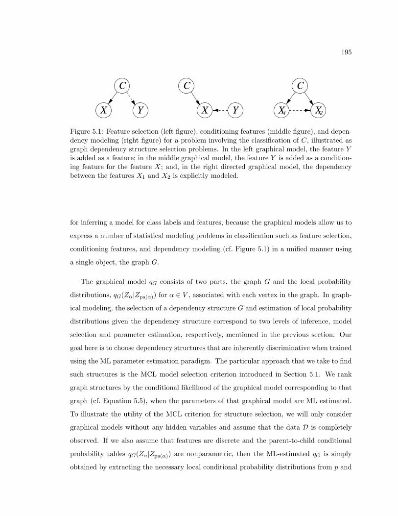
195
C
X Y Y
C
X
C
X X1 2
Figure 5.1: Feature selection (left figure), conditioning features (middle figure), and depen-dency modeling (right figure) for a problem involving the classification of C, illustrated asgraph dependency structure selection problems. In the left graphical model, the feature Yis added as a feature; in the middle graphical model, the feature Y is added as a condition-ing feature for the feature X; and, in the right directed graphical model, the dependencybetween the features X1 and X2 is explicitly modeled.
for inferring a model for class labels and features, because the graphical models allow us to
express a number of statistical modeling problems in classification such as feature selection,
conditioning features, and dependency modeling (cf. Figure 5.1) in a unified manner using
a single object, the graph G.
The graphical model qG consists of two parts, the graph G and the local probability
distributions, qG(Zα|Zpa(α)) for α ∈ V , associated with each vertex in the graph. In graph-
ical modeling, the selection of a dependency structure G and estimation of local probability
distributions given the dependency structure correspond to two levels of inference, model
selection and parameter estimation, respectively, mentioned in the previous section. Our
goal here is to choose dependency structures that are inherently discriminative when trained
using the ML parameter estimation paradigm. The particular approach that we take to find
such structures is the MCL model selection criterion introduced in Section 5.1. We rank
graph structures by the conditional likelihood of the graphical model corresponding to that
graph (cf. Equation 5.5), when the parameters of that graphical model are ML estimated.
To illustrate the utility of the MCL criterion for structure selection, we will only consider
graphical models without any hidden variables and assume that the data D is completely
observed. If we also assume that features are discrete and the parent-to-child conditional
probability tables qG(Zα|Zpa(α)) are nonparametric, then the ML-estimated qG is simply
obtained by extracting the necessary local conditional probability distributions from p and
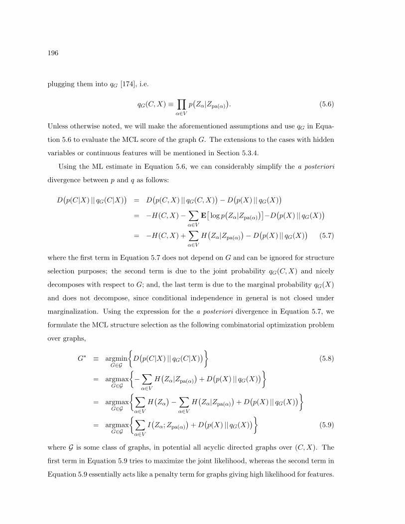
196
plugging them into qG [174], i.e.
qG(C,X) ≡∏α∈V
p(Zα|Zpa(α)
). (5.6)
Unless otherwise noted, we will make the aforementioned assumptions and use qG in Equa-
tion 5.6 to evaluate the MCL score of the graph G. The extensions to the cases with hidden
variables or continuous features will be mentioned in Section 5.3.4.
Using the ML estimate in Equation 5.6, we can considerably simplify the a posteriori
divergence between p and q as follows:
D(p(C|X) || qG(C|X)
)= D
(p(C,X) || qG(C,X)
)−D
(p(X) || qG(X)
)= −H(C,X)−
∑α∈V
E[log p
(Zα|Zpa(α)
)]−D
(p(X) || qG(X)
)= −H(C,X) +
∑α∈V
H(Zα|Zpa(α)
)−D
(p(X) || qG(X)
)(5.7)
where the first term in Equation 5.7 does not depend on G and can be ignored for structure
selection purposes; the second term is due to the joint probability qG(C,X) and nicely
decomposes with respect to G; and, the last term is due to the marginal probability qG(X)
and does not decompose, since conditional independence in general is not closed under
marginalization. Using the expression for the a posteriori divergence in Equation 5.7, we
formulate the MCL structure selection as the following combinatorial optimization problem
over graphs,
G∗ ≡ argminG∈G
{D(p(C|X) || qG(C|X)
)}(5.8)
= argmaxG∈G
{−∑α∈V
H(Zα|Zpa(α)
)+D
(p(X) || qG(X)
)}= argmax
G∈G
{∑α∈V
H(Zα
)−∑α∈V
H(Zα|Zpa(α)
)+D
(p(X) || qG(X)
)}= argmax
G∈G
{∑α∈V
I(Zα;Zpa(α)
)+D
(p(X) || qG(X)
)}(5.9)
where G is some class of graphs, in potential all acyclic directed graphs over (C,X). The
first term in Equation 5.9 tries to maximize the joint likelihood, whereas the second term in
Equation 5.9 essentially acts like a penalty term for graphs giving high likelihood for features.
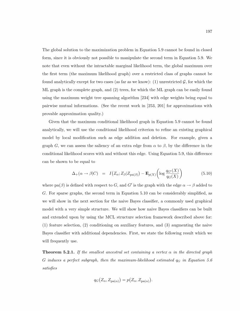
197
The global solution to the maximization problem in Equation 5.9 cannot be found in closed
form, since it is obviously not possible to manipulate the second term in Equation 5.9. We
note that even without the intractable marginal likelihood term, the global maximum over
the first term (the maximum likelihood graph) over a restricted class of graphs cannot be
found analytically except for two cases (as far as we know): (1) unrestricted G, for which the
ML graph is the complete graph, and (2) trees, for which the ML graph can be easily found
using the maximum weight tree spanning algorithm [234] with edge weights being equal to
pairwise mutual informations. (See the recent work in [253, 201] for approximations with
provable approximation quality.)
Given that the maximum conditional likelihood graph in Equation 5.9 cannot be found
analytically, we will use the conditional likelihood criterion to refine an existing graphical
model by local modification such as edge addition and deletion. For example, given a
graph G, we can assess the saliency of an extra edge from α to β, by the difference in the
conditional likelihood scores with and without this edge. Using Equation 5.9, this difference
can be shown to be equal to
∆+(α→ β|C) = I(Zα;Zβ|Zpa(β)
)−Ep(X)
(log
qG′(X)qG(X)
)(5.10)
where pa(β) is defined with respect to G, and G′ is the graph with the edge α→ β added to
G. For sparse graphs, the second term in Equation 5.10 can be considerably simplified, as
we will show in the next section for the naive Bayes classifier, a commonly used graphical
model with a very simple structure. We will show how naive Bayes classifiers can be built
and extended upon by using the MCL structure selection framework described above for:
(1) feature selection, (2) conditioning on auxiliary features, and (3) augmenting the naive
Bayes classifier with additional dependencies. First, we state the following result which we
will frequently use.
Theorem 5.2.1. If the smallest ancestral set containing a vertex α in the directed graph
G induces a perfect subgraph, then the maximum-likelihood estimated qG in Equation 5.6
satisfies
qG(Zα, Zpa(α)
)= p(Zα, Zpa(α)
).

198
(A vertex set in a directed graph is ancestral if the ancestors of all vertices in that set are
contained in that set. A directed graph is called perfect if the parent set induced subgraph
of each vertex is complete. See [174] for details. Notice that Equation 5.6 already states
that qG(Zα|Zpa(α)
)= p
(Zα|Zpa(α)
), and the only additional implication of Theorem 5.2.1
is that qG(Zpa(α)
)= p(Zpa(α)
).)
Proof. The proof directly follows from the following two facts [174]: (1) the marginal distri-
bution corresponding to any ancestral set factorizes with respect to the subgraph that they
induce, with the same conditional probability factors as those in the full joint distribution
in Equation 5.5, and (2) the ML estimate for a decomposable graphical model (cf. Equa-
tion 2.58) is found by setting the marginal distribution over each clique to the corresponding
marginal distribution in p. The first fact implies that the ML estimate for the conditional
probability factors corresponding to the variables in the ancestral set can be separately
found by solving the ML estimation problem for the ancestral-set induced subgraph. If this
subgraph is perfect as assumed in the theorem, then it can be expressed as a decomposable
graph by dropping the directionality of edges. In the resulting decomposable graph, each
vertex and its parents lie in the same clique, and the second fact implies the result of the
theorem. The theorem imposes the perfectness condition on the smallest ancestral set, since
if any ancestral set containing α is perfect, then the smallest ancestral set containing α is
also perfect.
If p entails some independence assumptions, then the perfectness condition can be con-
siderably relaxed.
5.3 Naive Bayes Classifier
The naive Bayes classifier is a simple yet competitive classifier which finds many uses in
applications such as medical diagnosis, text classification, etc. [197]. In a naive Bayes
classifier, the joint distribution over class label and features is modeled by assuming that
features are conditionally independent of each other when conditioned on the class label:
pNB(C,X1, . . . , XN ) ≡ p(C)N∏
i=1
p(Xi|C), (5.11)
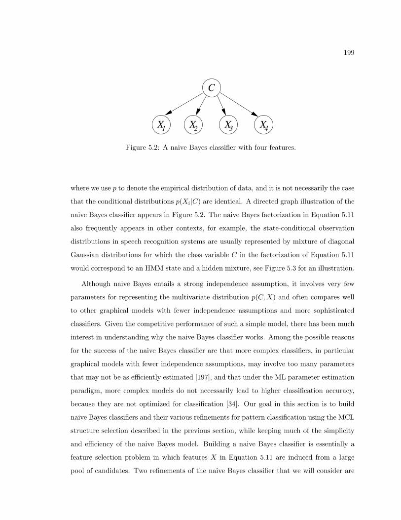
199
C
X1 X2 X3 X4
Figure 5.2: A naive Bayes classifier with four features.
where we use p to denote the empirical distribution of data, and it is not necessarily the case
that the conditional distributions p(Xi|C) are identical. A directed graph illustration of the
naive Bayes classifier appears in Figure 5.2. The naive Bayes factorization in Equation 5.11
also frequently appears in other contexts, for example, the state-conditional observation
distributions in speech recognition systems are usually represented by mixture of diagonal
Gaussian distributions for which the class variable C in the factorization of Equation 5.11
would correspond to an HMM state and a hidden mixture, see Figure 5.3 for an illustration.
Although naive Bayes entails a strong independence assumption, it involves very few
parameters for representing the multivariate distribution p(C,X) and often compares well
to other graphical models with fewer independence assumptions and more sophisticated
classifiers. Given the competitive performance of such a simple model, there has been much
interest in understanding why the naive Bayes classifier works. Among the possible reasons
for the success of the naive Bayes classifier are that more complex classifiers, in particular
graphical models with fewer independence assumptions, may involve too many parameters
that may not be as efficiently estimated [197], and that under the ML parameter estimation
paradigm, more complex models do not necessarily lead to higher classification accuracy,
because they are not optimized for classification [34]. Our goal in this section is to build
naive Bayes classifiers and their various refinements for pattern classification using the MCL
structure selection described in the previous section, while keeping much of the simplicity
and efficiency of the naive Bayes model. Building a naive Bayes classifier is essentially a
feature selection problem in which features X in Equation 5.11 are induced from a large
pool of candidates. Two refinements of the naive Bayes classifier that we will consider are
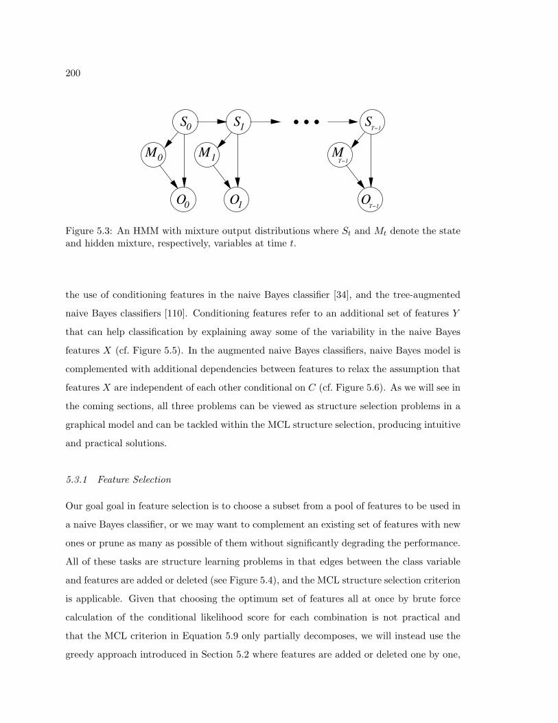
200
M0
S1 S...
0O
S0
O1
M1 MT−1
T−1
OT−1
Figure 5.3: An HMM with mixture output distributions where St and Mt denote the stateand hidden mixture, respectively, variables at time t.
the use of conditioning features in the naive Bayes classifier [34], and the tree-augmented
naive Bayes classifiers [110]. Conditioning features refer to an additional set of features Y
that can help classification by explaining away some of the variability in the naive Bayes
features X (cf. Figure 5.5). In the augmented naive Bayes classifiers, naive Bayes model is
complemented with additional dependencies between features to relax the assumption that
features X are independent of each other conditional on C (cf. Figure 5.6). As we will see in
the coming sections, all three problems can be viewed as structure selection problems in a
graphical model and can be tackled within the MCL structure selection, producing intuitive
and practical solutions.
5.3.1 Feature Selection
Our goal goal in feature selection is to choose a subset from a pool of features to be used in
a naive Bayes classifier, or we may want to complement an existing set of features with new
ones or prune as many as possible of them without significantly degrading the performance.
All of these tasks are structure learning problems in that edges between the class variable
and features are added or deleted (see Figure 5.4), and the MCL structure selection criterion
is applicable. Given that choosing the optimum set of features all at once by brute force
calculation of the conditional likelihood score for each combination is not practical and
that the MCL criterion in Equation 5.9 only partially decomposes, we will instead use the
greedy approach introduced in Section 5.2 where features are added or deleted one by one,
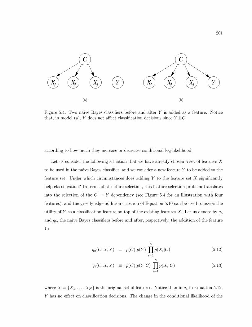
201
C
X1 X2 X3 Y
(a)
C
X1 X2 X3 Y
(b)
Figure 5.4: Two naive Bayes classifiers before and after Y is added as a feature. Noticethat, in model (a), Y does not affect classification decisions since Y⊥⊥C.
according to how much they increase or decrease conditional log-likelihood.
Let us consider the following situation that we have already chosen a set of features X
to be used in the naive Bayes classifier, and we consider a new feature Y to be added to the
feature set. Under which circumstances does adding Y to the feature set X significantly
help classification? In terms of structure selection, this feature selection problem translates
into the selection of the C → Y dependency (see Figure 5.4 for an illustration with four
features), and the greedy edge addition criterion of Equation 5.10 can be used to assess the
utility of Y as a classification feature on top of the existing features X. Let us denote by qa
and qb, the naive Bayes classifiers before and after, respectively, the addition of the feature
Y :
qa(C,X, Y ) ≡ p(C) p(Y )N∏
i=1
p(Xi|C) (5.12)
qb(C,X, Y ) ≡ p(C) p(Y |C)N∏
i=1
p(Xi|C) (5.13)
where X ≡ {X1, . . . , XN} is the original set of features. Notice than in qa in Equation 5.12,
Y has no effect on classification decisions. The change in the conditional likelihood of the
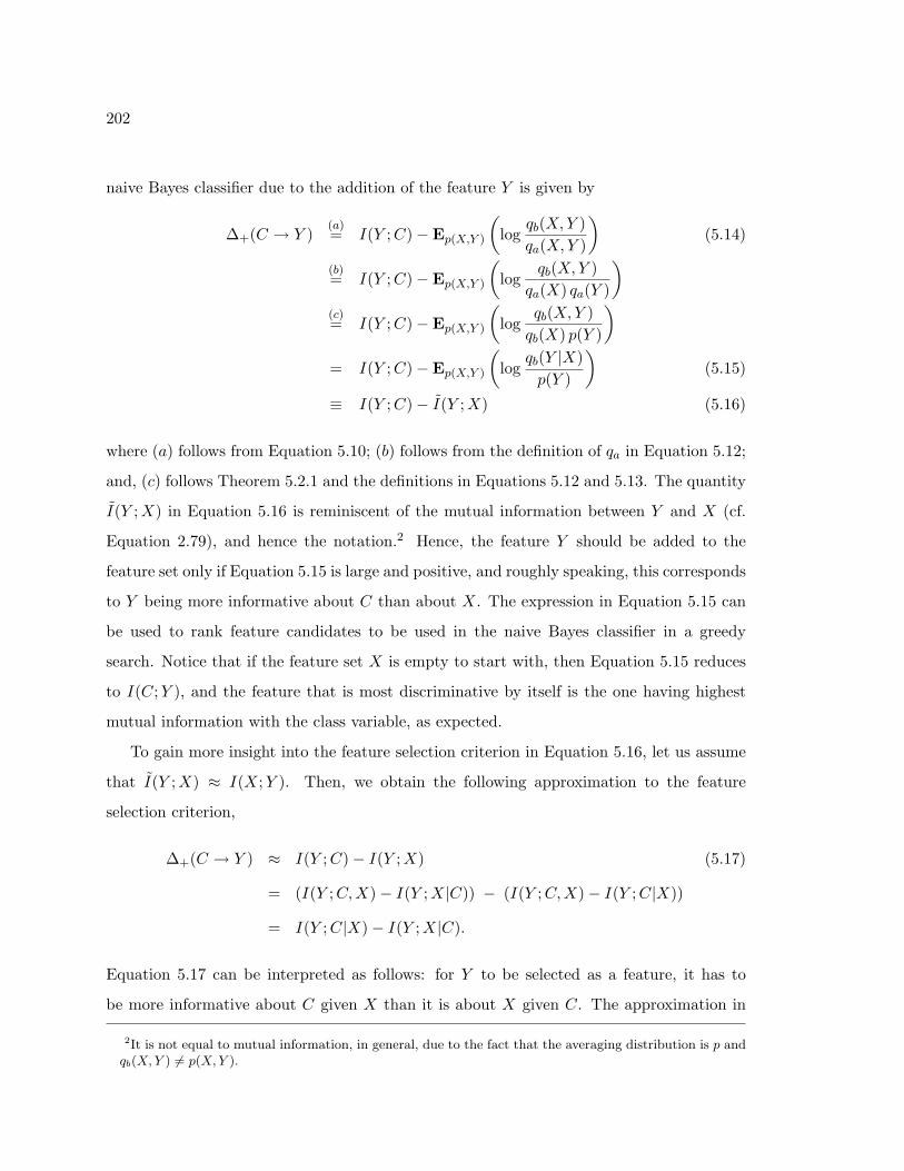
202
naive Bayes classifier due to the addition of the feature Y is given by
∆+(C → Y )(a)= I(Y ;C)−Ep(X,Y )
(log
qb(X,Y )qa(X,Y )
)(5.14)
(b)= I(Y ;C)−Ep(X,Y )
(log
qb(X,Y )qa(X) qa(Y )
)(c)= I(Y ;C)−Ep(X,Y )
(log
qb(X,Y )qb(X) p(Y )
)= I(Y ;C)−Ep(X,Y )
(log
qb(Y |X)p(Y )
)(5.15)
≡ I(Y ;C)− I(Y ;X) (5.16)
where (a) follows from Equation 5.10; (b) follows from the definition of qa in Equation 5.12;
and, (c) follows Theorem 5.2.1 and the definitions in Equations 5.12 and 5.13. The quantity
I(Y ;X) in Equation 5.16 is reminiscent of the mutual information between Y and X (cf.
Equation 2.79), and hence the notation.2 Hence, the feature Y should be added to the
feature set only if Equation 5.15 is large and positive, and roughly speaking, this corresponds
to Y being more informative about C than about X. The expression in Equation 5.15 can
be used to rank feature candidates to be used in the naive Bayes classifier in a greedy
search. Notice that if the feature set X is empty to start with, then Equation 5.15 reduces
to I(C;Y ), and the feature that is most discriminative by itself is the one having highest
mutual information with the class variable, as expected.
To gain more insight into the feature selection criterion in Equation 5.16, let us assume
that I(Y ;X) ≈ I(X;Y ). Then, we obtain the following approximation to the feature
selection criterion,
∆+(C → Y ) ≈ I(Y ;C)− I(Y ;X) (5.17)
= (I(Y ;C,X)− I(Y ;X|C)) − (I(Y ;C,X)− I(Y ;C|X))
= I(Y ;C|X)− I(Y ;X|C).
Equation 5.17 can be interpreted as follows: for Y to be selected as a feature, it has to
be more informative about C given X than it is about X given C. The approximation in
2It is not equal to mutual information, in general, due to the fact that the averaging distribution is p andqb(X, Y ) 6= p(X, Y ).

203
Equation 5.17 suggests that the utility of the feature Y given X is always less than or equal
to the information that it has about C given X. It can indeed be shown that ∆+(C → Y )
is less than or equal to I(Y ;C|X), if X involves a single feature:
∆1+(C → Y )
(a)= I(Y ;C)−Ep(X,Y )
(log
qb(X,Y )qa(X,Y )
)(b)= I(Y ;C)−Ep(X,Y )
(log
qb(X,Y )p(X) p(Y )
)(c)= I(Y ;C)−Ep(X,Y )
(log∑C∈C
p(C|X,Y )p(C|X,Y )
qb(C,X, Y )p(X) p(Y )
)(d)
≤ I(Y ;C)−Ep(C,X,Y )
(log
qb(C,X, Y )p(C|X,Y ) p(X) p(Y )
)(e)= I(Y ;C)−Ep(C,X,Y )
(log
p(C) p(X|C) p(Y |C)p(C|X,Y ) p(X) p(Y )
)= I(Y ;C) + I(Y,X;C)− I(X;C)− I(Y ;C)
= I(Y ;C|X)
where (a) is a repeat of Equation 5.14; (b) follows from the definition of qa in Equation 5.12
and that X only involves a single feature; (c) is a trivial identity to write the summation as
an expectation; (d) follows from Jensen’s inequality; (e) follows from the definition of qb in
Equation 5.12; and, the rest is straightforward algebra.
An expression similar to Equation 5.15 can be obtained for pruning away a feature
Y from the feature list. The deletion of a feature Y is equivalent to the removal of the
C → Y edge in the naive Bayes classifier, and the resulting change in the conditional log-
likelihood is the negative of that in Equation 5.15. Overall, the criterion in Equation 5.15
can be the basis of a feature selection algorithm as follows. Starting from an empty set of
features, one can first add as many features as possible until the feature addition criterion
does not significantly increase, and second prune away as many features as possible until
the feature deletion criterion does not significantly increase. Notice that since features are
chosen one by one, and each is conditional on previous ones, the resulting feature sets are
not necessarily jointly optimal. Also, the evaluation of the term I(Y ;X) in Equation 5.16
could be computationally very demanding for feature sets X with many features (N), as
it involves summing over N + 1 variables. If this is the case, a simple heuristic that could

204
be applicable is to calculate the saliency of the new feature Y with respect to each existing
feature Xi in the feature set using Equation 5.16 with X replaced by Xi and then choose
Y only if all of these pairwise saliencies are high. A more principled approach is to bound
the saliency in terms of single and pairwise information-theoretic quantities that can be
efficiently calculated (cf. Section 7.2).
5.3.2 Conditioning Features
Let us consider the naive Bayes model of Equation 5.11 but with the modification that we
have access to auxiliary or “side” information coming from another set of features Y ≡
{Y1, . . . , YM} that can potentially be used to increase the naive Bayes’s accuracy as follows.
We assume that Y by itself does not provide any information about the class C, i.e. Y
and C are marginally independent, but X is related to Y , and Y can explain some of the
variability observed in X that is not due to C. When X is conditioned on both C and
Y , we interpret C and Y as independent “causes” of X (see the left directed graphical
model in Figure 2.5 in Section 2.7.3 for an example). Such a structure can be useful for
classification of C, because Y might explain away X. The following example is from [218].
A house alarm (X) can go off either due to a burglary (C), or due to an earthquake (Y ).
If we only learn that alarm has went off, our belief that a burglary must have happened
increases; but once we learn that there was an earthquake, then we lower our belief for
burglary; thus, the earthquake explained away the alarm going off. Had we not represented
the information that earthquakes can also cause alarms going off, we would have incorrectly
concluded that the burglary is more likely than it actually is. However, we note that we do
not associate any causal semantics to our directed graphical models but use them only as a
tool for representing large dimensional probability distributions.
Conditioning the principal features X of a naive Bayes classifier on the auxiliary features
Y , we obtain the following factorization with respect to the modified naive Bayes graph:
q(C,X, Y ) ≡ p(C) p(Y )N∏
i=1
p(Xi|C, Y ∩Xpa(i)
)(5.18)
Notice that Xi takes C and potentially some empty subset in Y as parents, and hence
Xpa(i) = C ∪(Y ∩Xpa(i)
). Also, as we intended, C and Y are marginally independent

205
X1 X2 X3 X4
C
Y Y1 2
(a)
X1 X2 X3 X4
C
Y Y1 2
(b)
Figure 5.5: Two naive Bayes classifiers with principal features X and auxiliary features Y ,before and after X2 is conditioned on Y1.
according to Equation 5.18,
Under what circumstances are such conditionings of X on Y in the naive Bayes classifier
useful for predicting C? Notice that if the feature set Y∩Xpa(i) includes many features, then
the conditional distribution p(Xi|C, Y ∩Xpa(i)
)involve exponentially many parameters that
cannot be reliably estimated, and yet not all such dependencies might be useful for predicting
C. The selection of auxiliary feature subsets to be conditioned on by the principal features
is a structure selection problem, and the MCL structure selection is applicable. Similar to
the feature selection in Section 5.3.1, the optimal conditioning pattern is not obvious, and
we take a greedy approach in which principal features X are conditioned on the auxiliary
features Y one by one. For example, let us consider Yj as a parent of Xi given that we have
already chosen a number of dependencies from Y to X (as represented by the parent sets
below). Let us denote the graphical models before and after the addition of an edge from
Yj to Xi by qa and qb, respectively:
qa(C,X, Y ) ≡ p(C)
(M∏l=1
p(Yl)
)p(Xi|C, Y ∩Xpa(i))
∏k 6=i
p(Xk|C, Y ∩Xpa(k)), (5.19)
qb(C,X, Y ) ≡ p(C)
(M∏l=1
p(Yl)
)p(Xi|C, Yj , Y ∩Xpa(i))
∏k 6=i
p(Xk|C, Y ∩Xpa(k))(5.20)

206
where parent sets are with respect to the graph before the addition of the edge from Yj
to Xi. We will investigate the utility of using Yj as a conditioning feature for Xi by the
MCL edge addition criterion in Equation 5.10. We will start with the most general case
which does not assume anything about the structure of dependencies other than those in
Equations 5.19 and 5.20. In the general case, the change in the MCL score due to the
addition of the edge Yj → Xi is given by
∆+(Yj → Xi)(a)= I
(Yj ;Xi|C, Y ∩Xpa(i)
)−Ep(X,Y )
(log
qb(X,Y )qa(X,Y )
)(5.21)
(b)= I
(Yj ;Xi|C, Y ∩Xpa(i)
)−Ep(X,Y )
(log
qb(Xi|X−i, Y
)qa(Xi|X−i, Y
)) (5.22)
where X−i ≡ X\{Xi} (all X except Xi); (a) follows from Equation 5.10; and, (b) follows
from the fact that the smallest ancestral sets containing {X−i, Y } are identical before and
after the addition of the edge Yj → Xi (see the proof of Theorem 5.2.1). In general,
Equation 5.22 cannot be further simplified. (It is not the case that Xi⊥⊥Y |X−i in general,
since C and Y become dependent on each other when conditioned on X−i due to the
explaining away phenomenon.) To gain insight into Equation 5.22, we will now consider a
series of special cases. Let us first assume that Yj does not have any children other than Xi
before it is added as a parent of Xi. Then, we can simplify Equation 5.22 as
∆+(Yj → Xi) = I(Yj ;Xi|C, Y ∩Xpa(i)
)−Ep(X,Y )
(log
qb(Xi|X−i, Y−j , Yj)qa(Xi|X−i, Y−j
) )≡ I
(Yj ;Xi|C, Y ∩Xpa(i)
)− I(Yj ;Xi|X−i, Y−j
)(5.23)
where I is a quantity similar to the conditional mutual information between Yj and Xi given
all of the remaining principal and auxiliary features. Thus, roughly speaking, conditioning
Xi on Yj is useful only if the amount of information Yj contains about Xi is more when
conditioned on C than not conditioned.
Let us now consider the simplest nontrivial case involving only one conditioning feature
Y and one principal feature X. Then, the saliency criterion in Equation 5.22 simplifies to
∆1+(Y → X) = I(Y ;X|C)− I(Y ;X) (5.24)
≈ I(Y ;X|C)− I(Y ;X) (5.25)
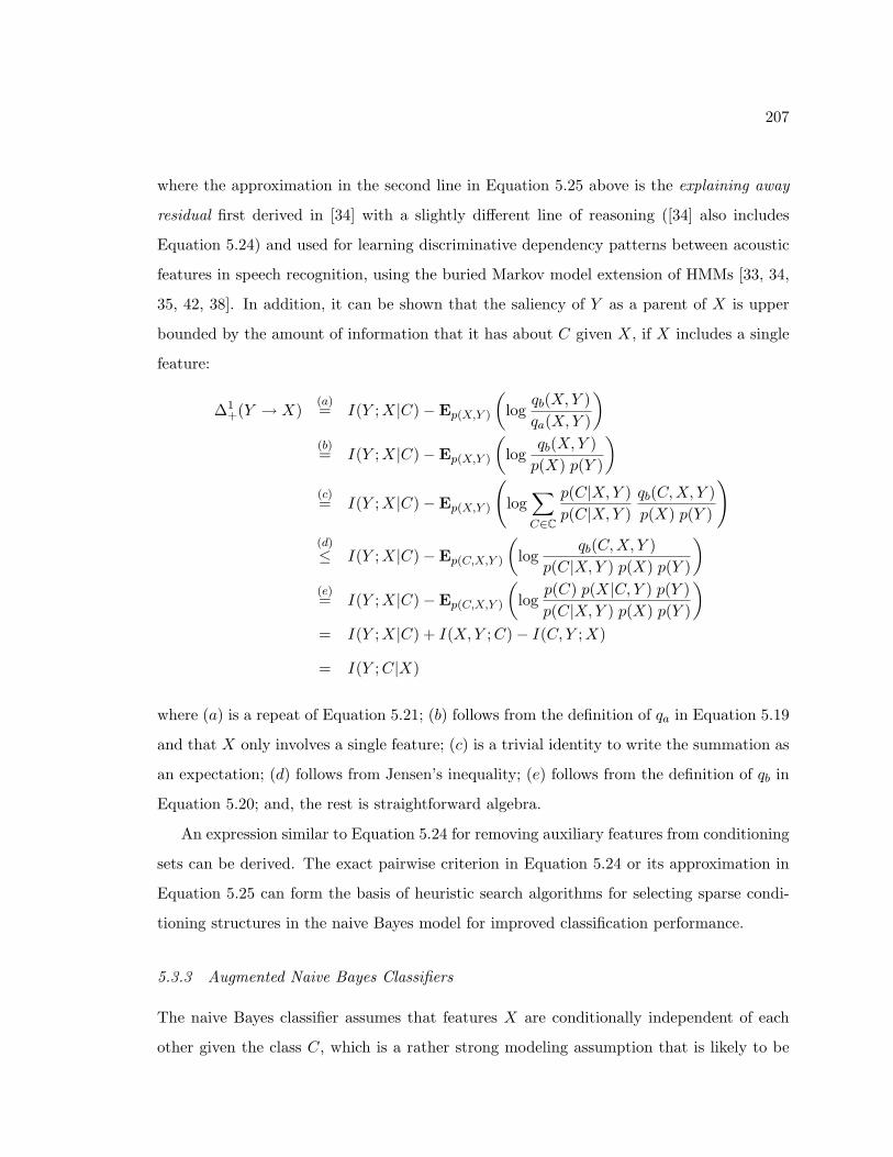
207
where the approximation in the second line in Equation 5.25 above is the explaining away
residual first derived in [34] with a slightly different line of reasoning ([34] also includes
Equation 5.24) and used for learning discriminative dependency patterns between acoustic
features in speech recognition, using the buried Markov model extension of HMMs [33, 34,
35, 42, 38]. In addition, it can be shown that the saliency of Y as a parent of X is upper
bounded by the amount of information that it has about C given X, if X includes a single
feature:
∆1+(Y → X)
(a)= I(Y ;X|C)−Ep(X,Y )
(log
qb(X,Y )qa(X,Y )
)(b)= I(Y ;X|C)−Ep(X,Y )
(log
qb(X,Y )p(X) p(Y )
)(c)= I(Y ;X|C)−Ep(X,Y )
(log∑C∈C
p(C|X,Y )p(C|X,Y )
qb(C,X, Y )p(X) p(Y )
)(d)
≤ I(Y ;X|C)−Ep(C,X,Y )
(log
qb(C,X, Y )p(C|X,Y ) p(X) p(Y )
)(e)= I(Y ;X|C)−Ep(C,X,Y )
(log
p(C) p(X|C, Y ) p(Y )p(C|X,Y ) p(X) p(Y )
)= I(Y ;X|C) + I(X,Y ;C)− I(C, Y ;X)
= I(Y ;C|X)
where (a) is a repeat of Equation 5.21; (b) follows from the definition of qa in Equation 5.19
and that X only involves a single feature; (c) is a trivial identity to write the summation as
an expectation; (d) follows from Jensen’s inequality; (e) follows from the definition of qb in
Equation 5.20; and, the rest is straightforward algebra.
An expression similar to Equation 5.24 for removing auxiliary features from conditioning
sets can be derived. The exact pairwise criterion in Equation 5.24 or its approximation in
Equation 5.25 can form the basis of heuristic search algorithms for selecting sparse condi-
tioning structures in the naive Bayes model for improved classification performance.
5.3.3 Augmented Naive Bayes Classifiers
The naive Bayes classifier assumes that features X are conditionally independent of each
other given the class C, which is a rather strong modeling assumption that is likely to be
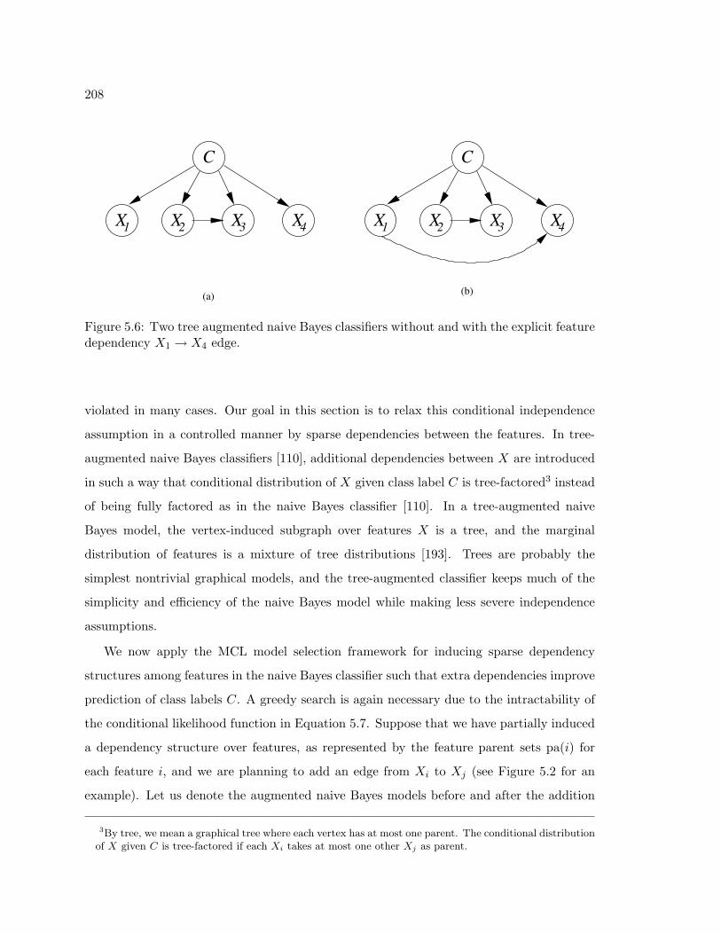
208
X1 X2 X3 X4
C
X1 X2 X3 X4
(a) (b)
C
Figure 5.6: Two tree augmented naive Bayes classifiers without and with the explicit featuredependency X1 → X4 edge.
violated in many cases. Our goal in this section is to relax this conditional independence
assumption in a controlled manner by sparse dependencies between the features. In tree-
augmented naive Bayes classifiers [110], additional dependencies between X are introduced
in such a way that conditional distribution of X given class label C is tree-factored3 instead
of being fully factored as in the naive Bayes classifier [110]. In a tree-augmented naive
Bayes model, the vertex-induced subgraph over features X is a tree, and the marginal
distribution of features is a mixture of tree distributions [193]. Trees are probably the
simplest nontrivial graphical models, and the tree-augmented classifier keeps much of the
simplicity and efficiency of the naive Bayes model while making less severe independence
assumptions.
We now apply the MCL model selection framework for inducing sparse dependency
structures among features in the naive Bayes classifier such that extra dependencies improve
prediction of class labels C. A greedy search is again necessary due to the intractability of
the conditional likelihood function in Equation 5.7. Suppose that we have partially induced
a dependency structure over features, as represented by the feature parent sets pa(i) for
each feature i, and we are planning to add an edge from Xi to Xj (see Figure 5.2 for an
example). Let us denote the augmented naive Bayes models before and after the addition
3By tree, we mean a graphical tree where each vertex has at most one parent. The conditional distributionof X given C is tree-factored if each Xi takes at most one other Xj as parent.

209
of this edge by qa and qb, respectively:
qa(C,X) ≡ p(C) p(Xj |Xpa(j), C
) ∏k 6=j
p(Xk|Xpa(k), C
)(5.26)
qb(C,X) ≡ p(C) p(Xj |Xi, Xpa(j), C
) ∏k 6=j
p(Xk|Xpa(k), C
)(5.27)
where the parent sets are defined with respect to the graph before the addition of the edge
Xi → Xj , and we use pa(i) with a slight abuse of notation to denote the parents of Xi only
in the vertices corresponding to X (the only other parent of each Xi is C). The difference
between the conditional likelihood scores of these two models can be used to assess the
utility of the edge Xi → Xj for predicting C:
∆+(Xi → Xj)(a)= I
(Xi;Xj |C,Xpa(j)
)−Ep(X)
(log
qb(X)qa(X)
)(5.28)
(b)= I
(Xi;Xj |Xpa(j), C
)−Ep(X)
(log
qb(Xj , Xde(j)|Xnd(j)
)qa(Xj , Xde(j)|Xnd(j)
)) (5.29)
where de(j) and nd(j), with an abuse of notation, denote those descendants and non-
descendants, respectively, of feature Xj that are in X (see Section 2.7.1 for definitions).
The equality (a) above follows from Equation 5.10, and (b) follows from the fact that the
smallest ancestral sets containing Xnd(j) are identical before and after the addition of the
edge Xi → Xj . In general, it is difficult to simplify Equation 5.29 since the features X
are dependent on each other via both C and augmented dependencies among themselves.
To gain insight into Equation 5.29, let us consider the following simple situation where the
edge Xi → Xj is appended to the naive Bayes model. Then, Equation 5.29 simplifies to
∆+(Xi → Xj) = I(Xi;Xj |C
)−Ep(X)
(log
qb(Xj |X−j)qa(Xj |X−j)
)(a)= I
(Xi;Xj |C
)−Ep(X)
(log
qb(Xj |X−j)qb(Xj |X−ij)
qa(Xj |X−ij)qa(Xj |X−j)
)≡ I
(Xi;Xj |C
)−(Ib(Xi;Xj |X−ij
)− Ia
(Xi;Xj |X−ij
))(5.30)
where X−ij ≡ X\{Xi, Xj}, and (a) follows from qb(X−i) = qa(X−i) due to Theorem 5.2.1.
The quantities Ib and Ia are reminiscent of the mutual information between Xi and Xj
conditional on remaining features, evaluated with and without, respectively, a direct de-
pendency between Xi and Xj (note that X−i = X−ij ∪ {Xj}). Thus, a direct dependency
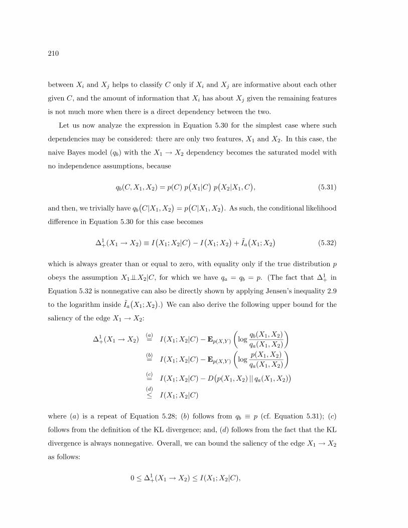
210
between Xi and Xj helps to classify C only if Xi and Xj are informative about each other
given C, and the amount of information that Xi has about Xj given the remaining features
is not much more when there is a direct dependency between the two.
Let us now analyze the expression in Equation 5.30 for the simplest case where such
dependencies may be considered: there are only two features, X1 and X2. In this case, the
naive Bayes model (qb) with the X1 → X2 dependency becomes the saturated model with
no independence assumptions, because
qb(C,X1, X2) = p(C) p(X1|C
)p(X2|X1, C
), (5.31)
and then, we trivially have qb(C|X1, X2
)= p(C|X1, X2
). As such, the conditional likelihood
difference in Equation 5.30 for this case becomes
∆1+(X1 → X2) ≡ I
(X1;X2|C
)− I(X1;X2
)+ Ia
(X1;X2
)(5.32)
which is always greater than or equal to zero, with equality only if the true distribution p
obeys the assumption X1⊥⊥X2|C, for which we have qa = qb = p. (The fact that ∆1+ in
Equation 5.32 is nonnegative can also be directly shown by applying Jensen’s inequality 2.9
to the logarithm inside Ia(X1;X2
).) We can also derive the following upper bound for the
saliency of the edge X1 → X2:
∆1+(X1 → X2)
(a)= I(X1;X2|C)−Ep(X,Y )
(log
qb(X1, X2)qa(X1, X2)
)(b)= I(X1;X2|C)−Ep(X,Y )
(log
p(X1, X2)qa(X1, X2)
)(c)= I(X1;X2|C)−D
(p(X1, X2) || qa(X1, X2)
)(d)
≤ I(X1;X2|C)
where (a) is a repeat of Equation 5.28; (b) follows from qb ≡ p (cf. Equation 5.31); (c)
follows from the definition of the KL divergence; and, (d) follows from the fact that the KL
divergence is always nonnegative. Overall, we can bound the saliency of the edge X1 → X2
as follows:
0 ≤ ∆1+(X1 → X2) ≤ I(X1;X2|C),
211
implying that the saliency of this edge is always nonnegative and less than or equal to the
amount of information that X1 has about X2 when C is known. Comparing Equations 5.32
and 5.25, the saliency in Equation 5.32 can be interpreted as a modified explaining away
criterion, by an amount Ia(X1, X2) due to the existing edge C → X1. We note that if q
is parametrically modeled, which is almost always the case for continuous features, it is no
longer true that the conditional likelihood increases due to the edge X1 → X2. In any case,
the criterion in Equation 5.32 can be used to rank the utility of candidate dependencies in
an approximate search for sparse discriminative dependency structures.
The conditional likelihood score of a graphical model qG is only determined by its con-
ditional distribution qG(C|X), and as such, two graphical models with the same conditional
distribution qG(C|X) are equivalent according to the MCL criterion and hence so are those
with the same joint distribution. In the example we just considered, adding the edge
Xj → Xi instead of the edge Xi → Xj would result in the same ML-estimated joint dis-
tribution and receive a score identical to Equation 5.30 because the graphical models they
produce are Markov equivalent.4 Two Markov equivalent directed graphs would result in
the same ML-estimated distribution, since we assumed that all variables in our graphs are
discrete and that parent-to-child conditional probabilities are nonparametric. Also, if fea-
tures were continuous and their class-conditional distributions q(X|C = c) were represented
by multivariate Gaussian distributions, this would still be the case.
5.3.4 Extensions
There are some obvious extensions to the work presented here, some of which we will employ
in our experiment in Section 5.5.
First, we limited our attention to completely observed data, in particular the graphical
models that we considered did not involve any hidden variables, which excludes many in-
teresting models such as Gaussian mixture models and hidden Markov models. A simple
solution that we will employ to deal with hidden variables is to use the configuration having
4Two directed acyclic graphs are said to be Markov equivalent, if they have the same skeleton (theundirected graph obtained by dropping the directionality of all edges) and the v-structures (α → γ ← βwith no edge between α and β). Two Markov equivalent graphs imply exactly the same set of conditionalindependence properties [174].
212
the highest a posteriori probability, obtained from a baseline model, as if they were the
truly generated versions.
Second, we made no parametric modeling assumptions in the parent-to-child conditional
distributions, but such assumptions pose no particular difficulty, though they might not be
true, causing additional inaccuracies. Once the ML-estimated parametric distributions are
obtained by using the EM algorithm or some other method, the conditional likelihood
scores can be evaluated by using these parametric distributions. For example, in arriving
at Equation 5.32, we made use of a nonparametric modeling assumption. Without these
assumptions, the conditional likelihood score for the dependency considered in Equation 5.32
would become
∆1+(X1 → X2) = Ep
(log
qb(X2|X1, C
)qa(X2|C)
)−Ep
(log
qb(X2|X1
)qb(X2)
qb(X2)qa(X2|X1
))≡ ˜Ib(X1;X2|C)− ˜Ib(X1;X2) + ˜Ia(X1;X2) (5.33)
(Above we used the fact that the same parent-to-child conditional probability, q(X1|C) in
particular, appearing in two different graphical models would be estimated identically (and
hence q(X1) since q(C) is identical in both models), which is true for ML estimation when
there are no hidden variables, regardless of parametric vs. nonparametric modeling.)
Third, we implicitly assumed that each class-conditional distribution qG(X|C = c) is
graphical with respect to the same graph structure determined by the original graph G.
For example, each class-conditional distribution q(X|C = c) in the tree-augmented naive
Bayes model factors with respect to the tree over features. As we do in our applications,
this modeling assumption can be relaxed to use a different graph structure Gc for each
class-conditional distribution [35], the so-called Bayesian multinet approach in graphical
modeling. The conditional likelihood structure selection criteria can easily be modified
to accommodate the multinet approach where a different graph dependency structure for
each class-conditional distribution is chosen. For example, the analog of the conditional
likelihood score in Equation 5.33 (which evaluates the saliency of the edge X1 → X2 in all
class-conditional distributions) for a Bayesian multinet in which that edge is only used in

213
the c-th class-conditional distribution is
∆1+(X1 → X2|C = c) = Ep
(log
qb(X2|X1, C = c)qa(X2|C = c)
)−Ep
(log
qb(X1, X2)qa(X1, X2)
)(5.34)
≡ ˜Ib(X1;X2|C = c)− ˜Ib(X1;X2) + ˜Ia(X1;X2) (5.35)
because it holds that
I(X;Y |C) =∑c∈C
p(C = c) I(X;Y |C = c)
and that the last two terms in Equation 5.33 does not depend on C explicitly and can be
trivially written as an average with weights p(C = c), as above.
Fourth, the maximum conditional likelihood criterion can also overfit, as with all other
selection criteria based on data, and some form of regularization could be necessary to
penalize graphs with too many dependencies. A parameter penalty similar to the one used
in the minimum description length can be applied to the conditional log-likelihood scores.
Alternatively, hypothesis testing (cf. Section 2.8.2) can be used for determining whether or
not the conditional-likelihood increase due to a more complex structure is significant.
5.4 Comparison to Previous Work
Structure learning in graphical models is an active research topic, and there is a vast lit-
erature about it, mostly likelihood-based from a data description perspective, as reviewed
in Section 2.8.5 (for a through review, see, e.g. [264, 56, 142]). However, the problems of
likelihood-based structure selection criteria for classification tasks have long been recog-
nized. In [110], it is noted that the MCL criterion is better suited to the structure learning
of directed graphical model classifiers than the ML criterion, but there is no formal math-
ematical justification as in here in Section 5.2. In [170], the MCL criterion is used for
feature selection in the naive Bayes classifier. The concept of structural discriminability is
first introduced in [34, 35, 42], where the MCL criterion is used to enhance HMMs with
discriminative direct dependencies between observation vectors, using the explaining away
residual in Equation 5.25. In [34], it is also mentioned that the MCL criterion can be used
for learning the structure of a generic graphical model, as we did here. In [133], the hybrid

214
MCL model selection with ML parameter estimation is used for searching discriminative
structures with Markov chain Monte Carlo search methods.
As compared to these previous efforts that also employ the MCL criteria for structure
selection in graphical models, our main contribution is a careful analysis of the form that
the MCL criterion takes under a ML parameter estimation paradigm and interpreting the
simplified results for three modeling problems in the naive Bayes classifier: feature selection,
conditioning features, and augmented feature dependencies.
5.5 An Application to Speech Recognition for Acoustic Modeling
Multi-stream models of speech combine information extracted from multiple sources to
improve recognition accuracy, as we have seen in Section 4.3.2 for the 2-stream acoustic
modeling using PLP and HAT features. The information sources are multiple sequences of
features which have been derived either from the audio signal itself, e.g. PLPs and HATs,
or from some associated signal such as the video of speaker’s mouth in audio-visual speech
recognition [184].
In the basic multi-stream model involving two feature sequences, two HMMs are coupled
through their state sequences:
p({O1
t }T−1t=0 ,
{S1
t
}T−1
t=0,{O2
t
}T−1
t=0,{S2
t
}T−1
t=0
)≡
T−1∏t=0
p(S1
t |S1t−1
)p(O1
t |S1t
)p(S2
t |S2t−1, S
1t
)p(O2
t |S2t
)(5.36)
where T is the sequence length,{S1,2
t
}T−1
t=0are the state sequences in streams 1 and 2, and{
O1,2t
}T−1
t=0are the associated observation sequences. See Figure 4.4 for a graphical model
illustration of the 2-stream model. The observation streams in the multi-stream model
are not independent, but they are conditionally independent given their respective state
sequences. They depend on each other through the coupling of hidden state sequences, as-
suming conditional independence of observations given the underlying state sequences [209].
In the past work [34, 271], data-driven corpus studies have consistently shown that similar
temporal conditional independence assumptions in a feature stream modeled by HMMs do
not hold, and there lies significant information between current and surrounding observa-
215
tions conditional on the underlying state sequence label. Here we question the assumption
of conditional independence of observations extracted from time slices centered around the
same time using different windows and signal processing methods. Such independence as-
sumptions discards any direct dependencies among feature streams, which are potentially
discriminative for the underlying state sequences.
We extend the multi-stream model in Equation 5.36 to allow for such direct dependencies
between the observation streams. Even though an arbitrary selection of dependencies always
increases the descriptive power of the model, i.e. the likelihood, such an increase does not
necessarily translate into higher speech recognition accuracy, since the likelihood function
is not discriminative, as we discussed in Section 5.1. Thus, only dependencies which make
the model more discriminative should be chosen, and in this section, we investigate whether
such discriminative dependencies exist in the speech recognition task that we will consider
(sh5 task, cf. Section 3.1.6) and then incorporate those direct cross-stream observation
dependencies into the multi-stream model. Unlike previous work [196] that finds no evidence
of loss of discriminative information by the state-conditional independence assumption of
streams, we show that there does exist such discriminative information in direct cross-stream
dependencies, and that they can be exploited to improve speech recognition accuracy in the
sh5 task.
In the coupled HMMs described above, any dependence between the two observation
streams is mediated through the hidden state variables. This assumption might be too
simplistic for acoustic modeling given that O1,2t are derived from the same speech signal,
even if different signal processing methods are used.
5.5.1 Cross-stream Observation Dependencies
We extend the state-coupled HMM multi-stream model to allow direct dependencies from
one observation sequence to another, say from sequence 1 to sequence 2. Such direct de-
pendencies amount to replacing p(O2t |S2
t ) by p(O2t |O1
t , S2t ) in Equation 5.36. A graphical
model illustration of the extended dependencies is depicted in Figure 5.7. Due to their
mathematical tractability, we use mixtures of linear conditional Gaussians to implement
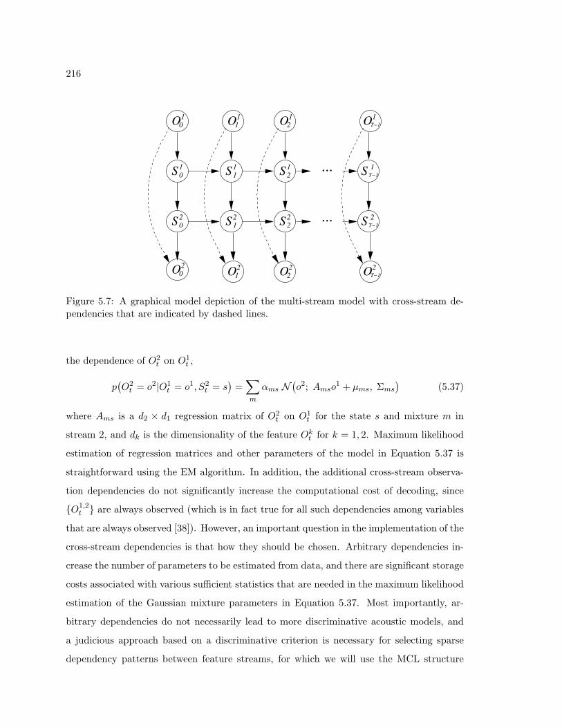
216
0O1
S0 S S2 2 2
O20O O12 2 2
1 2... 2
OT−12
S T−1
S0 S S1 2... S T−1
O2O1 OT−1
1 1 1 1
1 1 1
Figure 5.7: A graphical model depiction of the multi-stream model with cross-stream de-pendencies that are indicated by dashed lines.
the dependence of O2t on O1
t ,
p(O2
t = o2|O1t = o1, S2
t = s)
=∑m
αms N(o2; Amso
1 + µms, Σms
)(5.37)
where Ams is a d2 × d1 regression matrix of O2t on O1
t for the state s and mixture m in
stream 2, and dk is the dimensionality of the feature Okt for k = 1, 2. Maximum likelihood
estimation of regression matrices and other parameters of the model in Equation 5.37 is
straightforward using the EM algorithm. In addition, the additional cross-stream observa-
tion dependencies do not significantly increase the computational cost of decoding, since
{O1,2t } are always observed (which is in fact true for all such dependencies among variables
that are always observed [38]). However, an important question in the implementation of the
cross-stream dependencies is that how they should be chosen. Arbitrary dependencies in-
crease the number of parameters to be estimated from data, and there are significant storage
costs associated with various sufficient statistics that are needed in the maximum likelihood
estimation of the Gaussian mixture parameters in Equation 5.37. Most importantly, ar-
bitrary dependencies do not necessarily lead to more discriminative acoustic models, and
a judicious approach based on a discriminative criterion is necessary for selecting sparse
dependency patterns between feature streams, for which we will use the MCL structure
217
selection framework introduced in Section 5.2.
In the multi-stream model, the observation spaces are assumed to be independent of each
other when conditioned on the underlying states. In this sense, the multi-stream model is
analogous to the naive Bayes model with the joint state configuration in the multi-stream
model being the class variable C in the naive Bayes model, and the observation streams
being the features X in the naive Bayes model. With this interpretation of the multi-stream
model, the cross-stream dependency selection in the multi-stream model is similar to the
augmented feature dependencies in the naive Bayes model (cf. Equation 5.3.3), and we
use the augmented dependency selection criterion in Equation 5.35 for selecting additional
dependencies between the components of O1t and O2
t that are in the same time frame, for
each underlying state in stream 2. In the multi-stream acoustic models that we will consider,
each phone is context-dependently modeled in both streams using a three-state topology,
and the triphone states in each stream are separately tied using phone and state position
dependent decision trees. There are thousands of tied states with relatively small amount
of training data corresponding to each. To prevent the partitioning of training data among
many context-dependent states for the reliable estimation of information-theoretic quantities
in the selection criterion, we have used the following scheme to select dependency patterns
for the context-dependent states in the stream 2. We tied the dependency structures for
all context-dependent states corresponding to a particular phone and state position, and
such dependencies are selected to according to the multinet dependency selection criterion
in Equation 5.35,
∆1+(O1
i → O2j ) = ˜Ib(O1
i ;Oj2|PS)− ˜Ib(Oi
1;Oj2) + ˜Ia(Oi
1;Oj2) (5.38)
where PS denotes a particular phone label and state position, subscripts b and a denote
models with and without a dependency from the i-th component of the feature in stream 1
to the j-th component of the observation in stream 2. The information-theoretic quantities
in Equation 5.38 are calculated as follows. First, using a baseline HMM system we force-
aligned the training data into the context-dependent states in the system. Next, the state
labels in the forced alignments were reduced to the joint label of phone and state position,
that each tied state correspond to. For each phone and state position, and for each pair of
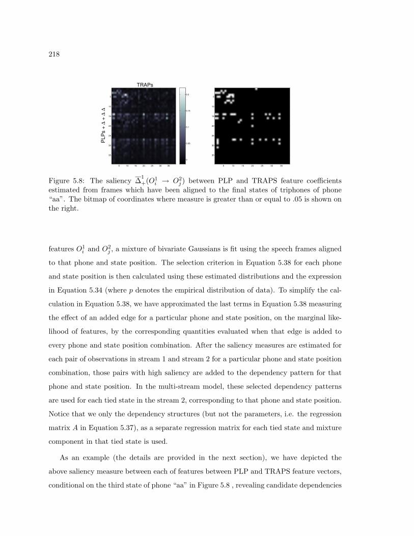
218
5 10 15 20 25 30 35
5
10
15
20
25
30
35
5 10 15 20 25 30 35
5
10
15
20
25
30
35
0
0.05
0.1
0.15
0.2
TRAPs
PLP
s +
∆ +
∆ ∆
Figure 5.8: The saliency ∆1+(O1
i → O2j ) between PLP and TRAPS feature coefficients
estimated from frames which have been aligned to the final states of triphones of phone“aa”. The bitmap of coordinates where measure is greater than or equal to .05 is shown onthe right.
features O1i and O2
j , a mixture of bivariate Gaussians is fit using the speech frames aligned
to that phone and state position. The selection criterion in Equation 5.38 for each phone
and state position is then calculated using these estimated distributions and the expression
in Equation 5.34 (where p denotes the empirical distribution of data). To simplify the cal-
culation in Equation 5.38, we have approximated the last terms in Equation 5.38 measuring
the effect of an added edge for a particular phone and state position, on the marginal like-
lihood of features, by the corresponding quantities evaluated when that edge is added to
every phone and state position combination. After the saliency measures are estimated for
each pair of observations in stream 1 and stream 2 for a particular phone and state position
combination, those pairs with high saliency are added to the dependency pattern for that
phone and state position. In the multi-stream model, these selected dependency patterns
are used for each tied state in the stream 2, corresponding to that phone and state position.
Notice that we only the dependency structures (but not the parameters, i.e. the regression
matrix A in Equation 5.37), as a separate regression matrix for each tied state and mixture
component in that tied state is used.
As an example (the details are provided in the next section), we have depicted the
above saliency measure between each of features between PLP and TRAPS feature vectors,
conditional on the third state of phone “aa” in Figure 5.8 , revealing candidate dependencies
219
and showing that there exists significant discriminative information between the two feature
streams which are not captured through state coupling. Note that most pairwise measures
are around zero – evidence that arbitrary selection of dependencies might not improve the
performance.
5.5.2 Experiments
Experiments are in the context of the sh5 task (cf. Section 3.1.6), a cross-domain speech
recognition task where training data consist of unrestricted vocabulary conversational speech
utterances whereas testing data are number sequences. Similar to our experiments in Sec-
tion 4.3.2, we use short-term spectral PLP coefficients and long-term TRAPS features as
observation streams. (In these set of experiments we used the original TRAPS [148, 144] as
described in Section 3.1.1 and not the HAT variation that we used in experiments in Chap-
ter 4.) All experiments are performed in GMTK; and, we used the same acoustic modeling
paradigms and training procedures as those described in Section 4.3.2 for training HMM
and 2-stream HMM systems except that word-internal triphones as opposed to cross-word
triphones are used and that we employed first-pass decoding instead of n-best list rescoring.
The HMM systems represent each context-dependent phone with a three-state left-to-right
topology. The 2-stream HMM phone models also use a similar topology in each stream, and
the two streams are forced to synchronize at phone boundaries, but in between a single-state
asynchrony is allowed (cf. Figure 4.5). As in Section 4.3.2, a separate state tying for each
stream is obtained from the corresponding HMM systems. The number of unique states
for PLP and TRAPS streams are 868 and 1105, respectively. The baseline HMM system
uses 32 mixture components per state output distribution, and the number of parameters
in each system is roughly made equivalent by adjusting the number of mixture components.
The sparse dependencies of the PLP stream on the TRAPS stream are selected through
the measure in Equation 5.38 and the procedure described in the previous section. The
forced alignments used in this procedure are with respect an HMM system using concate-
nated PLP and TRAPS features, and a mixture of four bivariate Gaussians are fit to each
pair of features in PLP and TRAPS streams for each phone and state position. Using the
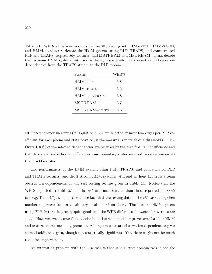
220
Table 5.1: WERs of various systems on the sh5 testing set. HMM-plp, HMM-traps,and HMM-plp/traps denote the HMM systems using PLP, TRAPS, and concatenatedPLP and TRAPS, respectively, features, and MSTREAM and MSTREAM+links denotethe 2-stream HMM systems with and without, respectively, the cross-stream observationdependencies from the TRAPS stream to the PLP stream.
System WER%
HMM-plp 3.8
HMM-traps 6.2
HMM-plp/traps 3.8
MSTREAM 3.7
MSTREAM+links 3.6
estimated saliency measures (cf. Equation 5.38), we selected at most two edges per PLP co-
efficient for each phone and state position, if the measure is more than a threshold (= .05).
Overall, 80% of the selected dependencies are received by the first five PLP coefficients and
their first- and second-order differences, and boundary states received more dependencies
than middle states.
The performances of the HMM system using PLP, TRAPS, and concatenated PLP
and TRAPS features, and the 2-stream HMM systems with and without the cross-stream
observation dependencies on the sh5 testing set are given in Table 5.1. Notice that the
WERs reported in Table 5.1 for the sh5 are much smaller than those reported for nsh5
(see e.g. Table 4.7), which is due to the fact that the testing data in the sh5 task are spoken
number sequences from a vocabulary of about 35 numbers. The baseline HMM system
using PLP features is already quite good, and the WER differences between the systems are
small. However, we observe that standard multi-stream model improves over baseline HMM
and feature concatenation approaches. Adding cross-stream observation dependencies gives
a small additional gain, though not statistically significant. Yet, there might not be much
room for improvement.
An interesting problem with the sh5 task is that it is a cross-domain task, since the
221
speaking styles of training (conversational) and testing (spoken numbers) data are consid-
erably different. Whether discriminative dependencies chosen on one type of data can still
be useful on some other type of data that is significantly different is an open question. It is
also an open question in general whether or not the MCL criterion is advantageous over the
ML criterion for such highly-mismatched data problems. (See Section 6.2.4 for more results
and a discussion on the effectiveness of MCL criterion for mismatched data in the context
of ML vs. MCL parameter estimation.)
We also note that our methodology for selecting cross-stream observation dependencies
makes a number of simplifications to reduce the computational cost, which might bias
the dependency selection criteria. First, the mutual information values used in structure
selection were evaluated by fitting a mixture of Gaussian distributions to the forced-aligned
state segmentations generated by an already trained HMM system. The use of a well-trained
HMM system for forced-alignments might bias or limit the contribution of cross-stream
dependencies in the multi-stream model, because the mutual information statistics used
in the saliency measures are estimated with respect to an HMM system not with respect
to the model to which cross-stream dependencies are applied, which is the multi-stream
model in our case. Second, in our dependency selection criterion in Equation 5.38, we have
only considered pairwise interactions between the feature streams, which might not be a
realistic assumption as there might exist higher-order interactions involving multiple feature
components in the two feature streams. Third, the multinet approximation in Equation 5.35
regarding the effect of a structure change in a class-conditional model on the marginal feature
distribution might not be accurate.
5.6 Summary
In this chapter we have proposed conditional likelihood function of class labels given clas-
sification features as a model selection criterion for pattern classification problems. Unlike
the joint likelihood function of class labels and features, emphasizing the description of
data (as used in traditional likelihood-based model selection methods), the conditional like-
lihood function emphasizes the prediction of class labels from features, and as such, it is
222
discriminative. We have used the maximum conditional likelihood criterion to formulate a
graph dependency algorithm for graphical model classifiers. The graphical modeling allows
expressing a number of statistical modeling problems in pattern classification using a single
object, the graph, and we have considered three such problems within the context of the
naive Bayes classifier: (1) feature selection, (2) conditioning features, and (3) dependency
modeling. We have carefully analyzed the particular form that the developed maximum
conditional likelihood model selection criterion takes for these problems. Particular atten-
tion has been given to the interaction between the commonly used maximum likelihood
parameter estimation at the first level and the proposed maximum conditional likelihood
model selection at the second level of statistical inference from data. For the three prob-
lems considered, this interaction has been carefully analyzed, and we show that the proposed
model selection criterion produces intuitive and practical solutions for these problems. The
utility of the maximum conditional likelihood structure selection algorithm lies in inferring
low-complexity discriminative models for pattern classification problems, and we have used
it for enhancing the multi-stream coupled HMMs, which are popularly used in acoustic
modeling for speech recognition, by direct cross-stream observation dependencies which are
not characterized in the basic models. We showed that in a cross-domain speech recognition
task, there exists discriminative information in the direct dependencies not represented by
the basic model, and those can be exploited to improve speech recognition accuracy.
223
Chapter 6
PARAMETER ESTIMATION FOR THE EXPONENTIAL FAMILY
In Chapter 5, we argued that the maximum conditional likelihood (MCL) criterion
is better suited for model selection in pattern classification problems than the maximum
likelihood (ML) criterion. The main point of our argument was that the MCL criterion uses
the free parameters of a model to minimize the mismatch between the true and model a
posteriori class distributions; as such, it can produce better classifiers than those produced
by the ML criterion; and, the resulting classifiers can be closer to the Bayes optimal classifier
in terms of both classification accuracy and confidence. This argument for the use of the
MCL criterion in model selection equally applies equally well to parameter estimation.
Indeed, discriminative parameter estimation methods such as maximum mutual information
estimation (which is equivalent to maximum conditional likelihood estimation when the class
a priori probabilities are kept fixed) are standard in large-vocabulary speech recognition,
see e.g., [256, 267].
The MCL criterion necessarily couples parameters from different classes by the nature
of its objective, and training data coming from all classes need to be considered when esti-
mating parameters for each class. Thus, the MCL parameter estimation is computationally
expensive. In addition, the parameter coupling in the conditional likelihood function oc-
curs in such a way that the mathematical methods commonly used in ML estimation such
as the lower-bound maximization in the EM algorithm (cf. Section 2.4) are not directly
applicable. However, there exist EM-like iterative algorithms such as the extended Baum-
Welch algorithm [19] that are currently being used with success for the MCL training of
HMM-based acoustic models, but the proofs that are used to formulate these algorithms and
show convergence require very small learning rates in the resulting parameter updates. Yet,
in practice, it has been observed that convergence is achieved for relatively large learning
rates, and as such, there seems to be a gap between theory and practice of MCL estimation

224
methods, in particular the extended Baum-Welch algorithm.
In this chapter, we will develop a new mathematical approach to maximum conditional
likelihood estimation in the linear exponential that will shed some new light to the ex-
tended Baum-Welch algorithm and its convergence behavior. Our development is largely
based on concave-convex procedure [278], a general method for constructing iterative maxi-
mization algorithms, which is reviewed in the next section. For the MCL estimation in the
exponential family,1 we will first formulate an iterative algorithm, which involves solving
a convex optimization problem at each iteration and guaranteed to monotonically increase
the conditional likelihood function. These convex problems cannot be solved analytically in
general, but their fixed-points are the extended Baum-Welch updates. Most importantly,
our formulation immediately suggests ways for choosing fast learning rates in the MCL
updates, which are closely related to those found in the speech recognition literature [267],
and as such, it provides a theoretical justification for the current practice of discriminative
training. We will test the utility of the MCL parameter estimation algorithm as well as the
effectiveness of proposed learning rate schemes in a speaker verification task. Some of the
intermediate results in these developments will also have implications for the ML estima-
tion in the exponential family using the EM algorithm [87]. First, we will show that all EM
algorithms in the exponential family are exactly equivalent to a first-order gradient-descent
algorithm. Second, we will provide a family of algorithms for the ML estimation in the
exponential family, which are similar to the EM algorithm in form; the EM algorithm is a
point in this family; and, the family includes the variations to the EM algorithm, which are
slower than the EM algorithm, and which are potentially faster when the amount of missing
information is high.
Before we continue, let us briefly give a few definitions in convexity [50] that we will
frequently refer to. A set X is said to be convex, if ∀ x1, x2 ∈ X and ∀ λ ∈ [0, 1],
xλ ≡ λx1 + (1− λ)x2 ∈ X.
1From here on, all exponential families considered in this chapter are linear, unless otherwise explicitlysaid.

225
A function f(x) : X→ R with the convex domain X is said to be convex, if, ∀ λ ∈ [0, 1],
f(xλ) ≤ λf(x1) + (1− λ)f(x2).
If f is first-order differentiable, then f is convex if and only if, ∀ x1, x2 ∈ X,
f(x2) ≥ f(x1) + (x2 − x1)>∂f(x)∂x
∣∣∣∣x=x1
. (6.1)
If f is second-order differentiable and its Hessian
H(x) ≡ ∂2f(x)∂x ∂x>
is nonnegative definite, then it is convex. A function g is said to be concave, if (−g) is
convex.
6.1 Concave-Convex Procedure
Concave-convex procedure (CCCP)2 is a method to construct iterative algorithms that
are guaranteed to monotonically increase general optimization functions [277, 278]. CCCP
is applicable to a very large class of optimization problems, and many commonly known
algorithms including EM algorithm, generalized iterative scaling, and Sinkhorn’s algorithm,
and some loopy belief propagation algorithms are shown to be special cases of this procedure.
Our exposition here follows [278] except that we present it as a maximization method instead
of as a minimization method.
Consider a function f over a convex set X such that f(x) = fcave(x) + fvex(x) where
fcave and fvex are concave and convex, respectively, functions of x, which we assume to
be sufficiently differentiable. (Any function with a bounded second-order derivative can be
written as a sum of a convex and a concave function [278]). The following theorem defines
CCCP as a method to maximize f .
Theorem 6.1.1. The iterative algorithm defined as
x(i+1) = argmaxx∈X
{fcave(x) + (x− x(i))>
∂fvex(x)∂x
∣∣∣∣x=x(i)
}(6.2)
2The acronym CCCP does not seem to be consistent with the expansion, but we are using it to beconsistent with the key paper that introduced it [278].
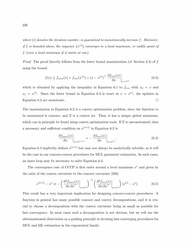
226
where (i) denotes the iteration number, is guaranteed to monotonically increase f . Moreover,
if f is bounded above, the sequence {x(i)} converges to a local maximum, or saddle point of
f (even a local minimum if it starts at one).
Proof. The proof directly follows from the lower bound maximization (cf. Section 2.4) of f
using the bound:
f(x) ≥ fcave(x) + fvex(x(i)) + (x− x(i))>∂fvex(x)∂x
∣∣∣∣x=x(i)
(6.3)
which is obtained by applying the inequality in Equation 6.1 to fvex with x2 = x and
x1 = x(i). Since the lower bound in Equation 6.3 is exact at x = x(i), the updates in
Equation 6.2 are monotonic.
The maximization in Equation 6.2 is a convex optimization problem, since the function to
be maximized is concave, and X is a convex set. Thus, it has a unique global maximum,
which can in principle be found using convex optimization tools. If X is unconstrained, then
a necessary and sufficient condition on x(i+1) in Equation 6.2 is
∂fcave(x)∂x
∣∣∣∣x=x(i+1)
= − ∂fvex(x)∂x
∣∣∣∣x=x(i)
. (6.4)
Equation 6.4 implicitly defines x(i+1) but may not always be analytically solvable, as it will
be the case in our concave-convex procedures for MCL parameter estimation. In such cases,
an inner loop may be necessary to solve Equation 6.4.
The convergence rate of CCCP is first order around a local maximum x∗ and given by
the ratio of the convex curvature to the concave curvature [238]:
x(i+1) − x∗ ≈ −(∂2fcave(x)∂x ∂x>
∣∣∣∣x=x∗
)−1(∂2fvex(x)∂x ∂x>
∣∣∣∣x=x∗
)(x(i) − x∗). (6.5)
This result has a very important implication for designing concave-convex procedures. A
function in general has many possible concave and convex decompositions, and it is cru-
cial to choose a decomposition with the convex curvature being as small as possible for
fast convergence. In most cases such a decomposition is not obvious, but we will use the
aforementioned observation as a guiding principle in devising fast-converging procedures for
MCL and ML estimation in the exponential family.

227
6.2 Maximum Conditional Likelihood Parameter Estimation
In this section, we will develop an iterative maximum conditional likelihood estimation algo-
rithm for the linear exponential family by devising a concave-convex procedure for maximiz-
ing the conditional likelihood function. The crux of this development is a concave-convex
decomposition for the conditional likelihood function, and the iterative estimation algo-
rithm will follow from Theorem 6.1.1 using this decomposition. We will first introduce this
algorithm in a simplified setting that each class-conditional distribution in the classification
problem is in the linear exponential family, possibly with hidden data. The linear exponen-
tial family is very rich and includes many important distributions such as Gaussian mixture
models (including those with spherical, or tied covariance matrices). However, HMMs with
left-to-right state transition topologies and other models which assign a zero probability to
a subset of sample space are not in the linear exponential family. To cover such models and
some other interesting models, we will later lift the restriction that class-conditional distri-
butions are in exponentially family and only assume that they can be written as mixtures of
such distributions. We will discuss the practical issue of choosing fast learning rates for the
proposed estimation algorithm based on insights from our derivation. We will then provide
a comparison of the work presented here to the previous work in discriminative training
and demonstrate the usefulness of the proposed algorithm in a speaker verification task,
where they are used for estimating the large-dimensional mixture of Gaussian speaker and
background models.
We remind the reader that a linear exponential family distribution is of the following
parametric form (cf. Section 2.5):
pθ(X = x) = c(x) exp{θ>t(x)− ψ(θ)
}(6.6)
where θ is the natural parameter, t(x) is the sufficient statistics, and ψ(θ) is the log-
normalization constant. The function c(x) in Equation 6.6 essentially determines the mea-
sure with respect to which pθ is a density, and without loss of any generality, we will assume
that it is absorbed into ψ(θ). We will also assume that θ is minimal, i.e. the components
of the components of θ as well as those of t(x) are linearly independent among themselves.
228
Assuming a minimal representation does not put any additional constraints on pθ, since any
non-minimal representation can be reduced to a minimal form by an appropriate transforma-
tion of parameters and sufficient statistics, but a minimal representation allows us to switch
back and forth between the natural parameter θ and the mean parameter η ≡ E[t(X)],
since they are one-to-one (cf. Section 2.5). In addition, we require θ ∈ Θ where Θ is convex
(cf. Equation 2.22). The log-normalization constant ψ(θ) is convex with derivatives (cf.
Equation 2.24):
∂ψ(θ)∂θc
= E [t(X)] , (6.7)
∂2ψ(θ)∂θc ∂θ>c
= cov [t(X)] . (6.8)
6.2.1 Algorithm Development
Consider the following classification problem where we predict the class C ∈ C using the
features Y ∈ Y. We assume that each class-conditional distribution pθc(Y = y|C = c) is of
the linear exponential family form with hidden data Z and complete data X ≡ (Y, Z):
pθc(Y = y|C = c) =∑z∈Z
exp{θ>c tc(x)− ψc(θc)
}. (6.9)
Notice that we do not assume that each class-conditional distribution pθ is of the same
parametric form. We want to estimate the parameters θ ≡ {θc}c∈C from a training set of
N examples, D ≡ {Cn, Yn}Nn=1, according to the maximum conditional likelihood criterion
(cf. Section 2.3.2). The conditional log-likelihood function of the parameters θ based on the
data D is given by
CL(θ;D) ≡N∑
n=1
(log p(Cn, Yn)− log p(Yn))
=∑
c
∑n:Cn=c
(log πc + log
(∑z
exp{θ>c tc(Xn)
})− ψc(θc)
)−∑
n
log(∑
c
πc
∑z
exp{θ>c tc(Xn)− ψc(θc)
})(6.10)
where πc denotes the a priori probability for class c; the first summation on the righthand
side is the joint likelihood of class labels and features; and, the second summation with the
229
negative sign is the marginal likelihood of features. The maximization of the conditional
likelihood function is difficult due to the negative summation term in Equation 6.10. On
the other hand, maximum likelihood estimation only involves maximization of the joint
likelihood function which nicely decouples across classes. In addition, the log-sum term in
the joint likelihood function does not pose much difficulty, as the application of Jensen’s
inequality gives a tractable, tight lower bound, which can be easily maximized to mono-
tonically increase the original joint likelihood function. The resulting algorithm is the EM
algorithm (cf. Section 2.4). However, when the same technique is used for the second sum-
mation with negative sign, it results in an upper bound due to the negative sign in front
of the logarithm, and maximizing such an upper bound does not necessarily increase the
conditional likelihood itself.
Instead, we will devise a concave-convex procedure to maximize the conditional like-
lihood function. For this purpose, we seek a concave and convex decomposition to the
conditional likelihood function in Equation 6.10 to which Theorem 6.1.1 will be applied. To
make the convergence as fast as possible, we want a decomposition with a convex part with
as small as possible curvature. Let us first rewrite Equation 6.10 as
CL(θ;D) = −∑
c
Nc ψc(θc) +∑
c
∑n:Cn=c
Fn(θc)−∑
n
Gn(θ) (6.11)
where we ignored the additive prior term in Equation 6.10, and
Fn(θc) ≡ log(∑
z
exp{θ>c tc(Xn)
})(6.12)
Gn(θ) ≡ log(∑
c
πc
∑z
exp{θ>c tc(Xn)− ψc(θc)
}). (6.13)
Now we will provide a concave-convex decomposition for each term in Equation 6.11, which
after an appropriate grouping, will translate into a concave-convex decomposition for the
conditional likelihood function itself. First, the log-normalization constant ψc(θc) in Equa-
tion 6.11 is convex by definition. Second, the following proposition shows that Fn(θc) in
Equation 6.11 is convex.
Proposition 6.2.1. Fn(θc) is convex in θc.

230
Proof. The proof follows from the fact the Hessian of Fn(θc) is nonnegative definite:
∂Fn(θc)∂θc
= E [tc(Xn)|Yn, Cn = c] , (6.14)
∂2Fn(θc)∂θc ∂θ>c
= cov [tc(Xn)|Yn, Cn = c] . (6.15)
Third, Gn(θ) in Equation 6.11 accepts the following concave-convex decomposition:
Gn(θ) =(−∑
c
Dc(n)ψc(θc))
+(Gn(θ) +
∑c
Dc(n)ψc(θc)), (6.16)
where the term inside first parentheses is concave due to convexity of ψc(θc), and the term
inside second parentheses is convex as proven by the following proposition.
Proposition 6.2.2. Hn(θ) ≡ Gn(θ) +∑
cDc(n)ψc(θc) is convex if Dc(n) ≥ 1 for all c.
Proof. The proof follows from the fact the Hessian of Hn(θ) is nonnegative definite:
∂Hn(θ)∂θc
= γc(n)E [tc(Xn)|Yn, Cn = c] +(Dc(n)− γc(n)
)ηc
∂2Hn(θ)∂θc ∂θ>c′
= δc,c′(Dc(n)− γc(n)
)cov [tc(Xn)|Cn = c]
+ δc,c′ γc(n)E[(tc(Xn)− ηc
) (tc(Xn)− ηc
)>|Yn, Cn = c]
− γc(n) γc′(n)(E [tc(Xn)− ηc|Yn, Cn = c]
)(E[tc(Xn)− ηc|Yn, Cn = c
])>(6.17)
which is nonnegative definite, because for any vector a of suitable dimension
a>∂2Hn(θ)∂θ ∂θ>
a =∑c,c′
a>c∂2Hn(θ)∂θc ∂θ>c′
ac′
=(∑
c
(Dc(n)− γc(n)
)a>c cov [tc(Xn)|Cn = c) ac
)+∑c,z
γcz(n)(a>c(tc(Xn)− ηc
))2−(∑
c,z
γcz(n) a>c(tc(Xn)− ηc
))2
=(∑
c
(Dc(n)− γc(n)
)a>c cov [tc(Xn)|Cn = c] ac
)+ var [ε(C,Z)|Yn]
≥ 0
where {ac} is a partitioning of a commensurate with θc, γcz(n) ≡ p(Cn = c, Zn = z|Yn), and
ε(C,Z) ≡ a>C(tc(Xn)−ηC
). Notice that the conditionDc(n) ≥ 1 ensures thatDc(n) ≥ γc(n)
over the whole parameter space Θ, while Dc(n) being independent of θ.
231
Using the convexity of ψc(θc) and Fn(θc), and the decomposition of Gn(θ) in Equa-
tion 6.16, we obtain the following concave-convex decomposition of the conditional likeli-
hood function in Equation 6.11, CL = CLcave + CLvex, where
CLcave(θ;D) = −(∑
c
Nc ψc(θc) +∑
n
Hn(θ))
(6.18)
CLvex(θ;D) =∑
c
∑n:Cn=c
Fn(θc) +∑
c
∑n
Dc(n)ψc(θc). (6.19)
In the concave-convex procedure, we will need the derivative of CLvex, which is given by
∂CLvex(θ;D)∂θc
=∑
n:Cn=c
E [tc(Xn)|Yn, Cn = c] +∑
n
Dc(n) ηc.
Now we are ready to state a concave-convex procedure for monotonically increasing the
conditional likelihood function in Equation 6.10. The theorem below is a repeat of Theo-
rem 6.1.1 applied to the conditional likelihood function with the concave and convex parts
in Equations 6.18 and 6.19, respectively. We define Θ ≡ ×c∈C Θc for θc ∈ Θc.
Theorem 6.2.1. The following iterates are guaranteed to monotonically increase the con-
ditional likelihood function:
θ(i+1) = argmaxθ∈Θ
{−(∑
c
Nc ψc(θc) +∑
n
Hn(θ))
+∑
c
θ>c
( ∑n:Cn=c
Eθ(i)c
[tc(Xn)|Yn, Cn = c] +∑
n
Dc(n) η(i)c
)}(6.20)
where Dc(n) ≥ 1 for all c and n. Moreover, the sequence {θ(i)} converges to a local maxi-
mum, or saddle point of the conditional likelihood function (even a local minima if it starts
at one).
The condition Dc(n) ≥ 1 in Theorem 6.2.1 comes from the proof that Equation 6.16 isa valid concave-convex decomposition for Gn(θ) (cf. Proposition 6.2.2). The guarantee forconvergence in Theorem 6.2.1 follows from the fact that the conditional likelihood is boundedfrom above unity. The iterates are guaranteed to monotonically increase the conditionallikelihood function of data at each iteration; and the optimization problem that needs to besolved at each iteration is convex; and as such, it has a unique global maximum. However,it cannot be solved analytically in general. Ignoring any constraints on the parameters for
232
the time being, we take derivatives in Equation 6.20 and set them to zero to obtain thefollowing set of equations in terms of mean parameters:
η(i+1)c =
Pn:Cn=c E
η(i)c
[tc(Xn)|Yn, Cn = c] −P
n γ(i+1)c (n)E
η(i+1)c
[tc(Xn)|Yn, Cn = c] +P
n Dc(n) η(i)c
Nc −P
t γ(i+1)c (n) +
Pn Dc(n)
which needs to be solved simultaneously for c ∈ C. These equations cannot be solved ana-lytically, but their form immediately suggest the following decoupled fixed-point iterationsby replacing all quantities on the right-hand side calculated with respect η(i+1) by thosecalculated according to η(i):
η(i+1)c =
Pn:Cn=c E
η(i)c
[tc(Xn)|Yn, Cn = c] −P
n γ(i)c (n)E
η(i)c
[tc(Xn)|Yn, Cn = c] +P
n Dc(n) η(i)c
Nc −P
t γ(i)c (n) +
Pn Dc(n)
.(6.21)
A couple of observations are in order. First, we note that the parameter update in Equa-
tion 6.21 is only approximate and not guaranteed to monotonically increase the conditional
likelihood function. Second, this update does not necessarily produce a valid mean param-
eter corresponding to some θc ∈ Θc, for example, when applied to estimation of a Gaussian
distribution it can result in negative variances. However, for large enough∑
nDc(n), the up-
date in Equation 6.21 can be guaranteed to produce a valid parameter η(i+1)c at the expense
of slower convergence, since the first and last terms in the numerator of Equation 6.21 are
valid mean parameters. Third, we note that the convergence rate of the updates in Equa-
tion 6.21 is determined by the constant∑
nDc(n). As∑
cDc(n) gets large, the convex
curvature (cf. Equation 6.19) increases, and the convergence slows down (cf. Equation 6.5).
If large, the parameters will not change from one iteration to the next, which is also obvious
from Equation 6.21. Thus, for each n, we want Dc(n) to be as small as possible. In our
derivation, we required that Dc(n) ≥ 1 for all c and n in Proposition 6.2.2, since this choice
guaranteed that Dc(n) ≥ γc(n) for any setting of parameters, and the smallest possible
such value is Dc(n) = 1. However, even Dc(n) = 1 could be a very conservative choice for
examples with very small γc(n), possibly for examples from classes other than c. A more
flexible choice based on γc(n) such as Dc(n) = ε+γc(n) or α ·γc(n) for some constant α > 1
might also be sufficient on average to maximize the conditional likelihood function, which
we will discuss in detail in the next section.

233
6.2.2 Extension to the Exponential Family Mixtures
The extension to the case in which each class-conditional distribution is expressed as a
mixture of linear exponential family distributions, as opposed to the full distribution being
in the linear exponential family is easily obtained as follows. Let us consider such a mixture
class-conditional distribution:
pθc(Y = y|C = c) =∑z∈Z
exp{θ>c tcz(x)− ψcz(θcz)
}. (6.22)
where each mixture component might be of a different parametric form, or might involve
extra layers of hidden variables which we collectively denote by Z. The MCL estimation
developed in the previous section for the case where the full class-conditional distributions
are in the exponential family, easily extends to the present case where they can be written
as mixtures of such distributions. The extension is derived by repeating the same steps
as before but with two modifications. First, we handle the joint likelihood term (analo-
gous to the first term Equation 6.10) by applying Jensen’s inequality to lower bound it
by a concave function of parameters; and second, we handle the marginal likelihood term
(analogous to the second term Equation 6.10) similar to the way that we handled it in
Equation 6.16, by adding and subtracting log-normalization constants from all classes and
mixture distributions, i.e.∑
cz Dcz(n)ψcz(θcz), where the condition on Dcz(n) is
Dcz(n) ≥ γcz(n) ≡ p(Zn = z, Cn = c|Yn). (6.23)
After these modifications, the update equation for the z-th mixture in the c-th class is given
by
η(i+1)cz =
∑n:Cn=c γ
(i)z|c(n) tcz(Yn, Zn = z) −
∑n γ
(i)cz (n) tcz(Yn, Zn = z) +
∑nDcz(n) η(i)
cz∑n:Cn=c γ
(i)z|c(n) −
∑n γ
(i)cz (n) +
∑nDcz(n)
(6.24)
where γ(i)z|c(n) ≡ pη(i)(Zn = z|Yn, Cn = c), and γ
(i)cz (n) ≡ pη(i)(Zn = z, Cn = c|Yn). We
note that it is also straightforward to extend the updates in Equation 6.21 or that in
Equation 6.24 to the cases where class or mixture distributions have tied parameters,3
by applying Jensen’s inequality to the joint likelihood function while handling the marginal
3Extension to the case with parameter tying is necessary to cover HMMs.
234
likelihood term with a concave-convex decomposition similar to Equation 6.16. For example,
the simple modification for HMMs with exponential family or mixture of exponential family
output distributions in Equation 6.16 is that the added and subtracted log-normalization
constants and the sufficient statistics are collected from the whole sequence, i.e. we require
Dc(n) ≥∑Tn−1
t=0 γc(t) for the n- observation sequence of length Tn, where γc(t) is the a
posteriori probability for state c, calculated from the forward-backward algorithm.
Let us consider a Gaussian mixture model (GMM) to represent each class-conditional
distribution,
p(Y = y|C = c) =M∑
z=1
αczN(y;µcz,Σcz
)(6.25)
where z denotes the hidden mixture component; M is the number of mixture components;
and, αcz, µcz, and Σcz are the mixture weight, mean, and covariance matrix, respectively,
associated with the z-th mixture component of the c-th class. The GMM in Equation 6.25
is in the linear exponential family (with hidden data), or, it can also be treated as a mixture
of exponential family distributions. If we take the latter approach, the update equations in
Equation 6.24 in terms of exponential family “mean” parameters η can be converted into
the usual GMM parameters in Equation 6.25:
α(i+1)cz =
∑n:Cn=c γ
(i)z|c(n)−
∑n γ
(i)cz (n) +Dc α
(i)cz
Nc −∑
n γ(i)c (n) +Dc
(6.26)
µ(i+1)cz =
∑n:Cn=c γ
(i)z|c(n)Yn −
∑n γ
(i)cz (n)Yn +Dcz µ
(i)cz∑
n:Cn=c γ(i)z|c(n)−
∑n γ
(i)cz (n) +Dcz
(6.27)
Σ(i+1)cz =
∑n:Cn=c γ
(i)z|c(n)Yn Y
>n −
∑n γ
(i)cz (n)Yn Y
>n +Dcz
(Σ(i)
cz + µ(i)cz
[µ
(i)cz
]>)∑n:Cn=c γ
(i)z|c(n)−
∑n γ
(i)cz (n) +Dcz
−µ(i+1)cz
(µ(i+1)
cz
)> (6.28)
where Dc ≡∑
nDc(n) and Dcz ≡∑
nDcz(n). If we take the former approach (i.e. treat
the GMM in Equation 6.25 as a linear exponential family distribution) then the resulting
updates according to Equation 6.21 are identical to Equations 6.26– 6.28 with Dcz replaced
by Dc (compare Equation 6.21 and Equation 6.24). The form of the parameter updates for
GMMs in Equations 6.26– 6.28 is similar to those in the extended Baum-Welch training [210,
235
256, 244, 267]. The main value of our developments is that it provides insight into choosing
optimal learning rates in the updates by considering each class and each example in the
data separately, which we will discuss next.
In the GMM updates in Equations 6.26– 6.28 care must be taken in the choice of Dc and
Dcz so that α(i+1)cz is nonnegative, and Σ(i+1)
cz is positive definite. In our implementation, if
any of the α(i+1)cz updates results in a negative mixture weight, we have doubled Dc starting
from its initial value (N), until all α(i+1)cz become positive. For the updates with non-
positive definite Σ(i+1)cz , we have simply floored Σ(i+1)
cz with a global covariance floor. We
have found that such variance flooring is more effective than increasing Dcz for maximizing
the conditional likelihood function, possibly due to the fact that Dcz is also used in updating
µ(i+1)cz which are unconstrained. At the (i+ 1)-th iteration, we have set Dcz as follows:
Dcz =c0M
∑n:Cn 6=c
γ(i)c (n) +
∑n:Cn 6=c
γ(i)cz (n), (6.29)
where c0 is set to c0 = 1 at the start of the training procedure, and it is doubled whenever
conditional likelihood decreases from one iteration to the next. The choice c0 = 1 and the
doubling of the learning rate at conditional likelihood drops were found to perform well
experimentally. The logic behind the choice of Dcz in Equation 6.29 is as follows. Roughly
speaking, the last term involving Dcz in the numerator of Equation 6.24 compensates for the
second term in the numerator appearing with a negative sign. For examples with Cn = c,
the first term in Equation 6.24 can compensate for the second term in Equation 6.24 since
γ(i)cz (n) ≤ γ(i)
z|c(n). For the remaining examples, for which Cn 6= c, the choice is
Dcz(n) =c0Mγ(i)
c (n) + γcz(n), (6.30)
so that the condition in Equation 6.23 will likely to be satisfied for the parameters θ near the
current parameters θ(i). Such dynamic choices based on the a posteriori class probabilities
are commonly used with success and absolutely essential for domains with large amounts of
data such as speech recognition. For example, a large vocabulary training corpus involves
millions of frames and thousands of classes, of which only a select subset have an appreciable
a posteriori weight on a given frame. We will demonstrate the effectiveness of such learning

236
rates in our experiments in Section 6.2.4 with the mixture of Gaussian speaker models in a
speaker verification task.
6.2.3 Comparison to Previous Work
MCL parameter estimation is popularly used in speech recognition, mainly as a discrimi-
native estimation method for the HMM-based acoustic models with mixture of Gaussian
output distributions [210, 256, 244, 267]. The update equations used in speech recognition
are similar to Equations 6.26, 6.27, and 6.28 in form and commonly referred to as extended
Baum-Welch training. The extended Baum-Welch training is introduced in [126] for the
maximization of general rational functions (e.g. conditional likelihood for discrete distri-
butions), which is later adapted to Gaussian distributions using a discrete approximation
to the Gaussian distribution. In [136], extended Baum-Welch estimation equations are di-
rectly derived for a large class of continuous distributions. The derivation in [126] and [136]
extending Baum-Welch training are essentially based on formulating a positive auxiliary
function for the conditional likelihood function and then maximizing of this auxiliary func-
tion using an algorithm similar to the EM algorithm. A global constant D analogous to Dcz
in Equation 6.27 appears in these derivations to ensure that the resulting auxiliary function
is positive everywhere in the parameter space. It is shown in [126] that such a finite D ensur-
ing such a positivity for discrete distributions can be found. Recently, in [167] and [16], the
existence of such a finite D for Gaussian distributions and exponential family distributions,
respectively, has been proven, but with no explicit expression. The extended Baum-Welch
training in the linear exponential family are similar to the TM algorithm [95], which max-
imizes a tilted version of the unconditional likelihood function (the marginal likelihood of
features in our set up). As compared to the derivations of the extended Baum-Welch updates
in [126, 136, 95], our results (cf. 6.2.1) establish these updates as fixed-points of a convex
optimization problem whose solutions are guaranteed to monotonically increase the condi-
tional likelihood function. However, the main value of our derivation lies in the fact that it
immediately suggests a way to choose optimal learning rates (cf. Dc(n) in Equation 6.21)
for the updates, which turns out to be closely related to the currently used learning rates in
237
speech recognition [267]. In addition, our derivation also allows for separate learning rates
for each mixture component (e.g. Dcz in Equations 6.26, 6.27, and 6.28), which is found to
be useful in practice [267]. Such finite and mixture-dependent learning rates do not follow
from the derivations in [126] and [136] (due to a global D). In [158, 157], an alternative
approach to maximizing conditional likelihood in the linear exponential family is taken by
finding a quadratic upper bound on the marginal likelihood term in Equation 6.10 (and
hence, a lower bound on the conditional likelihood function). For a probability distribution
involving a sequence of variables such as an HMM, the resulting quadratic lower bounds
tend to be loose and produce slowly converging updates. Such lower-bound maximization
techniques are also closely related to the lower bound method in [46] based on Taylor’s
theorem.
6.2.4 An Application to Speaker Verification
We applied the MCL parameter estimation algorithms developed in the previous sections
to the NIST 1996 speaker verification benchmark (cf. Section 3.2.5), where they are used
for discriminative training of mixture of Gaussian speaker and background models. For a
detailed description of the task (one-session condition in the benchmarks) and our verifi-
cation system that we use in our experiments, see Section 3.2. We represent each speaker
by a GMM and there is also a GMM to model impostors. The baseline speaker verifi-
cation system trains speaker and background models according to the ML criterion using
the EM algorithm, which we compared to the system that uses the MCL criterion. The
conditional likelihood function of training data is calculated by treating each speech frame
independently and evaluating its a posteriori probability against all other target and/or
background models. To initialize our MCL estimation, we used the ML estimated param-
eters just at the end of mixture splitting regime when the desired number of mixtures is
achieved (cf. Section 3.2.5), i.e. ML and MCL training methods are initialized identically.
For MCL estimation, we used Equations 6.26, 6.27, and 6.28 for parameter updates and
the learning rate in Equation 6.30 with c0 = 1 to start the training. The MCL training
is finished if either the relative conditional-likelihood increase drops below 10−4, or 250
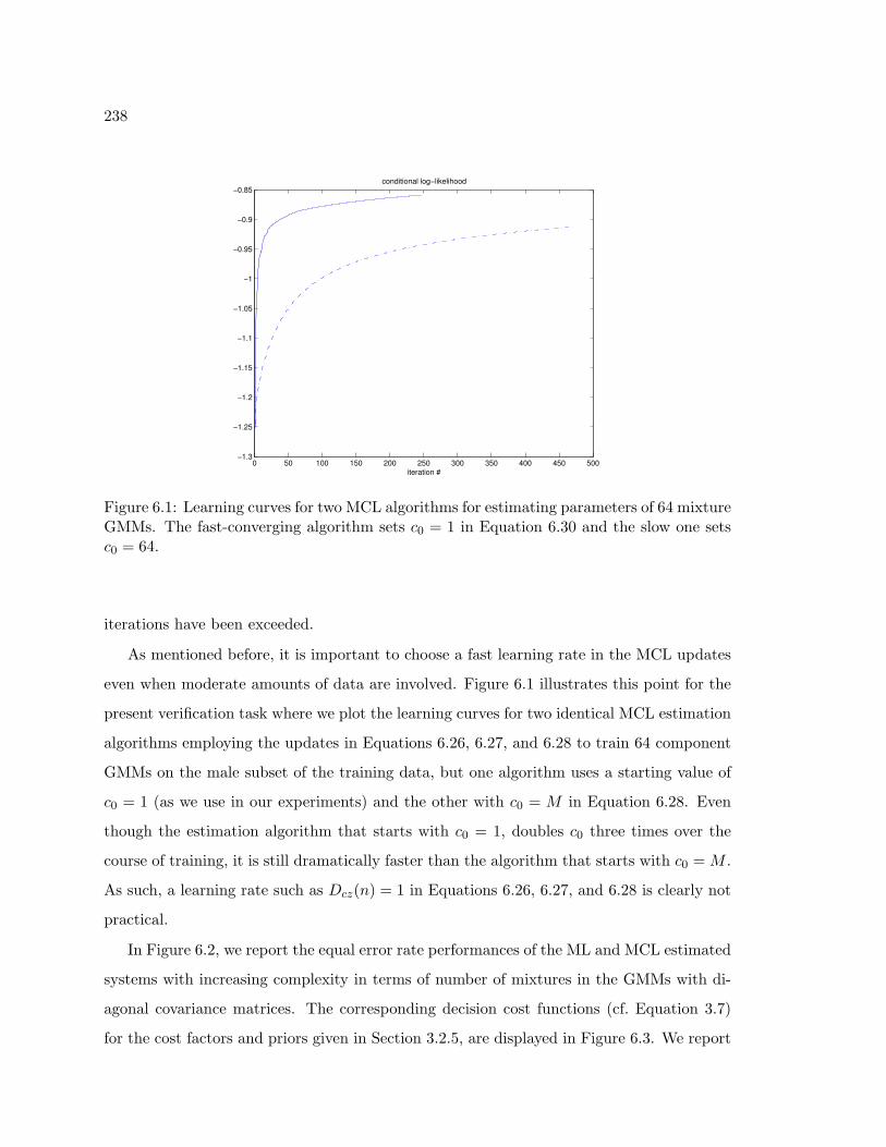
238
0 50 100 150 200 250 300 350 400 450 500−1.3
−1.25
−1.2
−1.15
−1.1
−1.05
−1
−0.95
−0.9
−0.85
iteration #
conditional log−likelihood
Figure 6.1: Learning curves for two MCL algorithms for estimating parameters of 64 mixtureGMMs. The fast-converging algorithm sets c0 = 1 in Equation 6.30 and the slow one setsc0 = 64.
iterations have been exceeded.
As mentioned before, it is important to choose a fast learning rate in the MCL updates
even when moderate amounts of data are involved. Figure 6.1 illustrates this point for the
present verification task where we plot the learning curves for two identical MCL estimation
algorithms employing the updates in Equations 6.26, 6.27, and 6.28 to train 64 component
GMMs on the male subset of the training data, but one algorithm uses a starting value of
c0 = 1 (as we use in our experiments) and the other with c0 = M in Equation 6.28. Even
though the estimation algorithm that starts with c0 = 1, doubles c0 three times over the
course of training, it is still dramatically faster than the algorithm that starts with c0 = M .
As such, a learning rate such as Dcz(n) = 1 in Equations 6.26, 6.27, and 6.28 is clearly not
practical.
In Figure 6.2, we report the equal error rate performances of the ML and MCL estimated
systems with increasing complexity in terms of number of mixtures in the GMMs with di-
agonal covariance matrices. The corresponding decision cost functions (cf. Equation 3.7)
for the cost factors and priors given in Section 3.2.5, are displayed in Figure 6.3. We report

239
0 50 10010
11
12
13
14
15
16
17T = 3
MA
TCH
ED
0 50 1008
9
10
11
12
13T = 10
0 50 1007
8
9
10
11
12T = 30
0 50 10018
19
20
21
22
23
24
MIS
MA
TCH
ED
0 50 10016
17
18
19
20
21
22
0 50 10016
17
18
19
20
21
22
Figure 6.2: The equal error rates (%) for ML (dashed) and CML (solid) estimated GMMspeaker and background models on the NIST 1996 speaker verification task (one-sessioncondition). The x-axis denotes the number of mixtures in the models; the rows correspondto the matched and mismatched, respectively, training/testing conditions, top to bottom;and the columns correspond to testing sets from utterances of 3, 10, and 30 seconds, left toright.
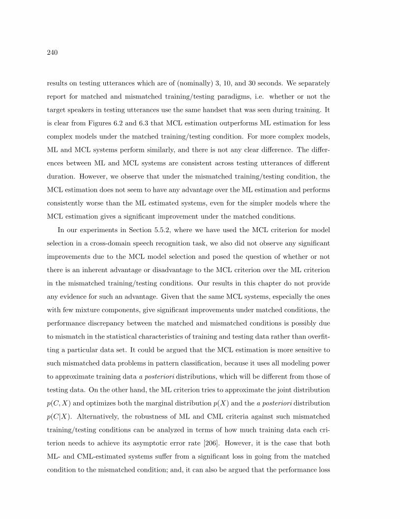
240
results on testing utterances which are of (nominally) 3, 10, and 30 seconds. We separately
report for matched and mismatched training/testing paradigms, i.e. whether or not the
target speakers in testing utterances use the same handset that was seen during training. It
is clear from Figures 6.2 and 6.3 that MCL estimation outperforms ML estimation for less
complex models under the matched training/testing condition. For more complex models,
ML and MCL systems perform similarly, and there is not any clear difference. The differ-
ences between ML and MCL systems are consistent across testing utterances of different
duration. However, we observe that under the mismatched training/testing condition, the
MCL estimation does not seem to have any advantage over the ML estimation and performs
consistently worse than the ML estimated systems, even for the simpler models where the
MCL estimation gives a significant improvement under the matched conditions.
In our experiments in Section 5.5.2, where we have used the MCL criterion for model
selection in a cross-domain speech recognition task, we also did not observe any significant
improvements due to the MCL model selection and posed the question of whether or not
there is an inherent advantage or disadvantage to the MCL criterion over the ML criterion
in the mismatched training/testing conditions. Our results in this chapter do not provide
any evidence for such an advantage. Given that the same MCL systems, especially the ones
with few mixture components, give significant improvements under matched conditions, the
performance discrepancy between the matched and mismatched conditions is possibly due
to mismatch in the statistical characteristics of training and testing data rather than overfit-
ting a particular data set. It could be argued that the MCL estimation is more sensitive to
such mismatched data problems in pattern classification, because it uses all modeling power
to approximate training data a posteriori distributions, which will be different from those of
testing data. On the other hand, the ML criterion tries to approximate the joint distribution
p(C,X) and optimizes both the marginal distribution p(X) and the a posteriori distribution
p(C|X). Alternatively, the robustness of ML and CML criteria against such mismatched
training/testing conditions can be analyzed in terms of how much training data each cri-
terion needs to achieve its asymptotic error rate [206]. However, it is the case that both
ML- and CML-estimated systems suffer from a significant loss in going from the matched
condition to the mismatched condition; and, it can also be argued that the performance loss
241
0 50 1004
4.5
5
5.5
6
6.5T = 3
MA
TCH
ED
0 50 1003
3.5
4
4.5
5
5.5T = 10
0 50 1002.5
3
3.5
4
4.5T = 30
0 50 1007.5
8
8.5
9
9.5
MIS
MA
TCH
ED
0 50 1007
7.5
8
8.5
0 50 1006.5
7
7.5
8
Figure 6.3: The decision cost functions (×100) for various ML (dashed) various CML(solid)estimated models on the NIST 1996 speaker verification task (one-session condition). SeeTable 6.2 for the legend.
242
under mismatched training/testing conditions is a common problem for classification algo-
rithms that infer probability distributions from data and use those estimated distributions
to make classification decisions [257].
6.3 EM Algorithm
In the previous section, we have devised a concave-convex procedure to maximize the con-
ditional likelihood function. Our goal in this section is to use concave-convex procedure to
develop a family of EM-type algorithms for the ML estimation in the exponential family.
The usual EM algorithm is one point in this family, and there are variants to the EM al-
gorithm, which are slower, as well as those which are potentially faster, especially in cases
where the amount of missing information is high. It is shown in [278] that all EM algo-
rithms are CCCP by applying a concave-convex decomposition to the auxiliary function of
the EM algorithm in terms of both the parameters and the averaging distribution (θ and
Q, respectively, see Equation 2.14). It is also mentioned in [278] that a formulation of the
EM algorithm in the linear exponential family in terms of natural parameters θ appears
in [115].
In this section, we will apply CCCP formulation directly to the likelihood function
instead of the auxiliary function of the EM algorithm as in [278]. The former approach
will be useful to gain insight to the convergence behavior of the EM algorithm as well as
developing variants of the EM algorithm with varying degrees of speed of convergence. Let
us consider the following maximum likelihood estimation problem in the exponential family.
We want to estimate the parameters of the model
pθ(X = x) ≡ exp{θ>t(x)− ψ(θ)
}(6.31)
using the incomplete data Y ≡ {Yn}Nn=1 corresponding to the complete data X ≡ {(Yn, Zn)}
with {Zn} missing. The (incomplete) log-likelihood function based on Y given by
L(θ;Y) ≡N∑
n=1
log(∑
z
exp{θ>t(x)
})− ψ(θ), (6.32)
which is difficult to optimize directly due to the log-sum term. Instead, the EM algo-
rithm iteratively maximizes the likelihood function via the following mapping of the mean
243
parameters from one iteration to the next one (cf. Section 2.5.2):
η(i+1)EM ≡ 1
N
∑n
Eη(i)EM
[t(Xn)|Yn = y] , (6.33)
where i denotes iteration number, and we use the subscript “EM”, to denote that parameters
estimated from the EM algorithm.
We will now derive a CCCP update for the ML estimation in the exponential family.
First we rewrite the likelihood function in Equation 6.32 as
L(θ;Y) =∑
n
(Fn(θ)− ψ(θ)
)(6.34)
where Fn(θ) is defined in Equation 6.12 and convex (cf. Proposition 6.2.1). We also know
that ψ(θ) is convex by definition. Thus, the likelihood function in Equation 6.32 accepts
the following concave-convex decomposition, L = Lcave + Lvex where
Lcave(θ;Y) ≡ −N(1 + α
)ψ(θ) (6.35)
Lvex(θ;Y) ≡∑
n
Fn(θ) +N αψ(θ) (6.36)
for any α such that α ≥ 0. We have introduced a free parameter α to control the convergence
rate in the CCCP updates below. Given the concave and convex parts in Equations 6.35
and 6.36, respectively, and the derivative of Fn(θ),
∂Fn(θ)∂θ
= E [t(Xn)|Yn] , (6.37)
we apply Theorem 6.1.1 (via Equation 6.4) to obtain the following CCCP updates that are
guaranteed to monotonically increase the likelihood function at each iteration:
η(i+1) =1
1 + α
(1N
Eη(i) [t(Xn)|Yn = y])
+α
1 + αη(i). (6.38)
We recognize the term in parentheses in Equation 6.38 as the would-be update of the EM
algorithm,
η(i+1)EM ≡ 1
N
∑n
Eη(i)
[t(Xn)|Yn = y] (6.39)
with the input parameter vector η(i) (see Equation 6.33). Thus, we can rewrite the CCCP
update in Equation 6.38 as
η(i+1) = λ η(i+1)EM + (1− λ) η(i) (6.40)
244
where λ = 11+α , satisfying λ ∈ (0, 1] for α ≥ 0. Using Equations 6.35 and 6.36, Equa-
tion 6.8, Equation 6.15, and Equation 6.5, we find that the convergence rate of the update
in Equation 6.40 around a local maximum η∗ is given by
η(i+1) − η∗ ≈(λ[Σ(i)X
]−1Σ(i)X|Y + (1− λ) I
)(η(i) − η∗) (6.41)
where I is an identity matrix of an appropriate dimension, and
Σ(i)X ≡ N covη(i)
[t(X)
]Σ(i)X|Y ≡
∑n
covη(i)
[t(Xn)|Yn
]which can be interpreted as the amount of complete and missing, respectively, information.
For α ≥ 0, the concave-convex decomposition in Equations 6.35 and 6.36 remains valid,
the update in Equation 6.40 based on such an α is guaranteed to monotonically increase
conditional likelihood. In particular, setting α = 0 (λ = 1) in Equations 6.40 and 6.41
recovers the usual EM algorithm and its convergence rate [87], respectively.
The CCCP update in Equation 6.40 has a very interesting interpretation. If α ≥ 0
(λ ∈ (0, 1]), the CCCP update at the (i+ 1)-th iteration is found by a convex combination
of the parameters from the EM algorithm’s would-be update at the current iteration and the
current parameters. As α increases, the ratio of convex curvature to the concave curvature
increases in Equation 6.35 and 6.36, and the convergence gets slower. The smallest α for
which our concave-convex decomposition is guaranteed to hold is α = 0 (λ = 1), which
recovers the usual EM algorithm. As such, the EM algorithm can be interpreted as the
fastest CCCP update in Equation 6.40 that can guarantee monotonic convergence. All
updates in Equation 6.40 based on α > 0 (λ ∈ (0, 1)) still guarantee monotonic convergence
of the likelihood but at a slower rate. The more interesting case is α ≤ 0 where the updates
in Equation 6.40 can potentially get much faster than that for α = 0. For −1 < α ≤ 0
(λ ≥ 1), the update in Equation 6.40 actually takes an over step along the direction of
the EM update, and a carefully chosen α ≤ 0 might decrease the ratio of convex curvature
to the concave curvature (and hence make the convergence faster) and still monotonically
increase the likelihood. For what kind of problems is the choice α ≤ 0 possible? An
insight is provided by the following analysis. All that we require from α is that (1) Lcave
245
in Equation 6.35 is concave, and (2) Lvex in Equation 6.35 is convex. The first condition
implies that α ≥ −1, so we only need to investigate the case −1 < α ≤ 0 (λ ≥ 1) for the
faster converging variants in Equation 6.40. Since we require that Lvex in Equation 6.36 is
convex, its second derivative needs to be nonnegative definite:
∂2Lvex(θ)∂θ ∂θ>
= Σ(i)X|Y + αΣ(i)
X . (6.42)
Thus, if Σ(i)X|Y is relatively large, i.e. the amount of missing information is large, then an
−1 < α ≤ 0 (λ ≥ 1) such that the expression in Equation 6.42 is locally positive definite is
possible. However, if Σ(i)X|Y is small, i.e. the amount of missing information is low, then the
choice α = 0 (λ = 1) is optimal. The effectiveness of such dynamic choices of α based on
the ratio of the missing information to the complete information in Equation 6.42, has been
experimentally verified in our experiments with GMMs (see Example 6.3.1), which is also
widely known since the inception of the EM algorithm, see e.g. [87, 153, 239]. As compared
to previous work in faster-converging variants of the EM algorithm, the CCCP updates in
Equation 6.40 in combination with a choice of λ based on Equation 6.42 keep simplicity of
the EM algorithm and provide a simple criterion to adjust the convergence rate or assess
when such modifications is feasible.
Example 6.3.1. We apply the CCCP updates in Equation 6.40 to a d-dimensional Gaus-
sian mixture model with M mixture components (cf. Equation 6.25). This model can be put
into the linear exponential family form (cf. Equation 6.31) as follows:
p(Z = z, Y = y) ≡ exp{θ>Z t(z) + t(z)> θZY t(y) + t(Z)> θZ − ψ(θZ , θZY , θZ)
}(6.43)
where the sufficient statistics t(z) have δz,z′ for z′ = 1, . . . ,M −1 as elements; the sufficient
statistics t(y) have yi and yiyj for i, j = 1, . . . , d as elements; and, θZ , θZY , and θY are
the natural parameters. In the training data, the mixture indicators Z are hidden, and we
estimate parameters based on samples from Y , using the CCCP update in Equation 6.40
with λ at the i-th iteration chosen according to Equation 6.42 as follows: we calculate Σ(i)X|Y
and Σ(i)X using the current set of parameters; we set α(i) in Equation 6.42 to the negative
half of the minimum generalized eigenvalue4 of Σ(i)X|Y and Σ(i)
X ; and, λ(i) = 11+α(i) . To reduce
4A generalized eigenvalue ζ and eigenvector v pair of A and B satisfies A v = ζ B v [139].
246
the computation, we use a block-diagonal approximation to Σ(i)X|Y , corresponding to θZ , and
the columns of θY Z .5 With this approximation, the calculation of Σ(i)X|Y and thus the CCCP
update in Equation 6.40 with λ set as described requires very little computation over that
which is necessary for the EM algorithm, and the speed comparisons between the CCCP and
EM algorithms can be directly made in terms total number of iterations until convergence.
We generate 10, 000 samples from a Gaussian mixture model with d = 16, M = 2d+ 1,
and parameters set as follows: the mixture weights in Equation 6.25 are uniformly set to 1M ;
the mean vector for the first mixture component is set to zero, for the (2 ·m)-th component
it is set to zero but +1 at the m-th dimension, and for the (2 ·m + 1)-th component it is
to zero but −1 at the m-th dimension; and, the covariance matrices are identically set to
σ2 I, where σ2 determines the overlap between mixture components and I is the identity
matrix. We only estimate mean vectors starting from an initialization where they are set
to one-fourth of their true values. Two sets of simulations, one with σ2 = 2 and the other
with σ2 = 1/2 are made, roughly corresponding to the cases where the amount of missing
information is high and low, respectively. The likelihoods for to the CCCP algorithms which
set λ dynamically as described above (the fast version), to constant 1 (the EM algorithm),
and to constant 1/2 (the slow version) are plotted in Figure 6.4. As can be seen from these
plots, the significant speed-ups from the CCCP updates with λ > 1 are possible in both cases
but much more so in the case where the amount of missing information is high (σ2 = 2)
than the case where it is low (σ2 = 1/2). We also find that even though the likelihoods are
not guaranteed to monotonically increase for the CCCP algorithms with λ > 1 (which is
always the case for the dynamic choices of λ, cf. Figure 6.4), in these examples, they do.
The plots in Figure 6.4 were typical across different simulations, and we found out that the
speed-ups from the CCCP algorithms are more pronounced when d is large.
Based on our previous results in this section, the following theorems about the EM
algorithm and the CCCP algorithm in Equation 6.40 can easily be proved. To simplify the
notation, we will assume N = 1 without loss of any generality.
5It is not necessary to calculate the components of Σ(i)
X|Y and Σ(i)X associated with θY , since the mean
parameter ηY ≡ E [t(Y )] can be directly estimated by setting ηY = 1N
PNn=1 t(Yn), cf. Equation 2.27.
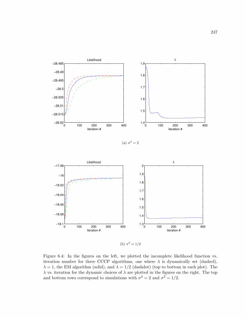
247
0 100 200 300 400−28.52
−28.515
−28.51
−28.505
−28.5
−28.495
−28.49
−28.485Likelihood
iteration #0 100 200 300 400
1.4
1.5
1.6
1.7
1.8
1.9λ
iteration #
(a) σ2 = 2
0 100 200 300 400−18.1
−18.08
−18.06
−18.04
−18.02
−18
−17.98Likelihood
iteration #0 100 200 300 400
1.3
1.4
1.5
1.6
1.7
1.8
1.9
2λ
iteration #
(b) σ2 = 1/2
Figure 6.4: In the figures on the left, we plotted the incomplete likelihood function vs.iteration number for three CCCP algorithms, one where λ is dynamically set (dashed),λ = 1, the EM algorithm (solid), and λ = 1/2 (dashdot) (top to bottom in each plot). Theλ vs. iteration for the dynamic choices of λ are plotted in the figures on the right. The topand bottom rows correspond to simulations with σ2 = 2 and σ2 = 1/2.
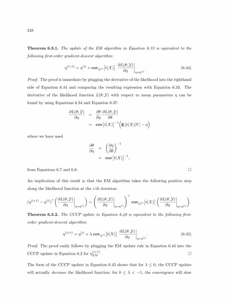
248
Theorem 6.3.1. The update of the EM algorithm in Equation 6.33 is equivalent to the
following first-order gradient-descent algorithm:
η(i+1) = η(i) + covη(i)
[t(X)
] ∂L(θ;Y)∂η
∣∣∣∣η=η(i)
. (6.44)
Proof. The proof is immediate by plugging the derivative of the likelihood into the righthand
side of Equation 6.44 and comparing the resulting expression with Equation 6.33. The
derivative of the likelihood function L(θ;Y) with respect to mean parameters η can be
found by using Equations 6.34 and Equation 6.37:
∂L(θ;Y)∂η
=∂θ
∂η
∂L(θ;Y)∂θ
= cov[t(X)
]−1(E [t(X)|Y ]− η
)where we have used
∂θ
∂η=
(∂η
∂θ
)−1
= cov[t(X)
]−1,
from Equations 6.7 and 6.8.
An implication of this result is that the EM algorithm takes the following positive step
along the likelihood function at the i-th iteration:
(η(i+1) − η(i))>(∂L(θ;Y)
∂η
∣∣∣∣η=η(i)
)=
(∂L(θ;Y)
∂η
∣∣∣∣η=η(i)
)>
covη(i)
[t(X)
](∂L(θ;Y)∂η
∣∣∣∣η=η(i)
).
Theorem 6.3.2. The CCCP update in Equation 6.40 is equivalent to the following first-
order gradient-descent algorithm:
η(i+1) = η(i) + λ covη(i)
[t(X)
] ∂L(θ;Y)∂η
∣∣∣∣η=η(i)
. (6.45)
Proof. The proof easily follows by plugging the EM update rule in Equation 6.44 into the
CCCP update in Equation 6.2 for η(i+1)EM .
The form of the CCCP update in Equation 6.45 shows that for λ ≤ 0, the CCCP update
will actually decrease the likelihood function; for 0 ≤ λ < −1, the convergence will slow
249
L
θ
.
θ(b)
(a)
Figure 6.5: Connected components of the likelihood function. An EM algorithm initializedat θ(a) is guaranteed to converge to the lower peak of the likelihood function and cannotconverge to the higher peak which does not lie in its connected component. On other hand,the algorithm initialized at θ(b) can potentially converge to either of the peaks.
down; for λ = 1, the CCCP update in Equation 6.45 is equivalent to the EM algorithm
update in Equation 6.44; and for λ > 1, the convergence might speed up. The choices λ > 1
are possible in problems when Σ(i)X|Y is large, i.e. the amount of missing data is high, e.g. in
a GMM estimation problem where mixtures highly overlap, as we have seen.
Theorem 6.3.3. Starting from initialization η(0), the EM updates in Equation 6.39 lie in
the set {η : L(η) ≥ L(η(0))}, connected component of the likelihood function, .
Proof. Assume otherwise that the EM algorithm produced a parameter η(i+1) at the i-
th iteration, which is not in the connected component of the set {η : L(η) ≥ L(η(0))}.
Then, according to the CCCP updates in Equation 6.40 for λ ∈ [0, 1], all parameters on
the line from the current parameters η(i) to the next parameters η(i+1) produce likelihoods
which are greater than the likelihood at the current iteration, which contradicts with the
condition that η(i+1) is not in the aforementioned connected component. See Figure 6.5 for
an illustration.
The above theorem is first proved in [195] for discrete EM algorithms. Our results generalize
it to all EM algorithms in the linear exponential family. The implication of this result is that
the EM algorithm is quite susceptible to poor initializations, which is empirically widely
known.
250
6.3.1 Comparison to Previous Work
The equivalence of the EM algorithm to a first-order gradient descent algorithm has been
previously established in [270] for the mixture of Gaussian distributions and in [240] for
the mixture of factor analyzers and HMMs. In [240], the equivalence between the EM
algorithm and a first-order gradient descent algorithm is also established for the general
exponential family in terms of natural parameters. As far as we know, this equivalence
expressed in the simplicity and generality of Theorem 6.3.1 in terms of mean parameters is
new. The relationships between the EM algorithm and the gradient-descent methods are
also explored in [44]. The family of EM-like algorithms defined in Theorem 6.3.2 includes
algorithms which converge slower or faster than the EM algorithm. The slower versions of
this family have been alternatively derived in [135] and applied to speaker adaptation with
very small amounts of data. In the cases where adaptation data are small, it is shown that
such partial maximization of the likelihood function gives better recognition performance
than full maximization.
Since the inception of the EM algorithm in [87], it has been long known that the EM
algorithm converges slowly if the amount of missing information is high as compared to
that of complete information. For such cases, various variants of the EM algorithm based
on Aitken acceleration methods [87], conjugate-gradient [153, 239], quasi-Newton numer-
ical optimization methods [154], and other methods [194] have been proposed. Recently,
in [238, 237] accelerations for a variety of bound optimization algorithms including the EM
algorithm, similar to the one in Theorem 6.3.2 have been formulated. As compared to these
works, the acceleration in Theorem 6.3.2 is similar to Aitken accelerations, and the main
utility of our formulation is that through it immediately suggests automatic way of choosing
the acceleration amount (cf. λ in Theorem 6.3.2 and Equation 6.42) and requires almost no
modification to the usual EM algorithm.
6.4 Summary
In this chapter we developed a new mathematical approach to maximum conditional like-
lihood parameter estimation in the exponential family using the concave-convex proce-

251
dure [278]. Based on the application of this optimization procedure to the conditional like-
lihood function, we first presented an iterative algorithm which is guaranteed to increase
conditional likelihood function at each iteration. The updates of this algorithm require solv-
ing a convex optimization problem at each iteration, which cannot be analytically obtained.
However, the fixed points of this problem provide a practical method for MCL estima-
tion, and the resulting updates are similar to the extended Baum-Welch updates which are
commonly used in acoustic model training for speech recognition. Most importantly, our
derivation suggests ways to choose fast learning rates in the resulting updates, which turned
out to be closely related to the currently used learning rates in speech recognition [267]. As
such, our analysis offers a theoretical justification for the current practice, which is missing
from the existing approaches. The application of the same mathematical tools that we used
to develop MCL estimation to the ML estimation allowed us to prove a few new results about
the EM algorithm and its variations. We showed that the EM algorithm is equivalent to
a first-order gradient-descent algorithm and developed faster-converging variants suggested
by the new analysis. We have demonstrated the viability of the faster-converging variants of
the EM algorithm for an estimation problem involving large-dimensional Gaussian mixture
models.
252
Chapter 7
CONCLUSIONS
The overall goal of this thesis was to design statistical models for pattern classification
problems, and we have made a number of contributions towards this goal. First, we de-
veloped a multi-scale extension of HMMs for modeling multi-scale stochastic processes and
applied them to machine tool-wear condition monitoring and acoustic modeling for speech
recognition. Second, we formulated a model selection criterion for statistical classifiers,
where models are chosen based on how useful they are for classification. This formula-
tion was used to select dependency structures for graphical model classifiers and applied to
acoustic modeling for speech recognition. Third, we developed a mathematical approach
to both maximum likelihood and maximum conditional likelihood parameter estimation for
the exponential family. These estimation methods were applied to speaker verification.
In the sections below, we will briefly review our main contributions, describe some of the
limitations of our approaches, and give future research directions suggested by our work.
7.1 Contributions and Conclusions
7.1.1 Multi-rate Hidden Markov Models
Multi-rate HMMs are a multi-scale extension to HMMs for characterizing temporal processes
evolving at multiple time scales. A multi-rate HMM decomposes a stochastic process into
scale-based parts and characterizes both the temporal evolution within each scale-based
part as well as the inter-scale couplings between these parts using scale-based state and
observation spaces. State and observation spaces are hierarchically organized from coarser
scales to finer ones, which allows for the simultaneous representation of both short- and long-
term context information. A multi-rate HMM consists of parallel HMMs which are coupled
through their hidden states. Due to its sparse modeling structure, multi-rate HMMs can
253
parsimoniously represent complex data, and their training and decoding are computationally
efficient. We also formulated two extensions to this basic model structure for (1) allowing
variable-rate sampling of coarser observation sequences, and (2) increased coupling between
scale-based parts by cross-scale observation and state dependencies. In combining evidence
from scale-based parts, multi-rate HMMs do not overcount evidence from coarser scales, and
as such, they provide better confidence values in classification problems. We have applied
multi-rate HMMs to two classification tasks, machine tool-wear monitoring and acoustic
modeling for speech recognition.
In machine tool-wear monitoring, we have used multi-rate HMMs for characterizing vi-
bration signatures of tools with various amount of wear in the context of milling titanium.
Titanium milling exhibits long-term “noisy/quiet” transient behavior for which a multi-rate
modeling approach is more appropriate. Classification results on real titanium milling data
set showed that multi-rate HMMs provide equal or better classification accuracy than the
corresponding HMM methods and outperform them in terms of the confidence of classifica-
tion decisions.
We have also applied multi-rate HMMs to acoustic modeling for speech recognition. The
current paradigm in speech recognition focuses on acoustic variability at the phone level
using short-term spectral features extracted from less than 100 msec windows. However,
contexts longer than phones such as syllables are also important for speech recognition,
and they contain information, such as lexical stress, that is complimentary to those in
phones and short-term spectral features. To utilize the information in modeling units bigger
than phones and features extracted from longer time scales, we used multi-rate HMMs for
two-scale acoustic modeling of speech with two different coarse scale alternatives: the one
where both coarse and fine scales represent phones, and the other where the fine scale
represents phones and the coarse scale represents syllable structure and stress. The speech
recognition experiments on a subset of a recent speech recognition benchmark (the 2001
Hub-5 evaluations) showed that the multi-rate HMMs gave significant improvements over
the traditional HMM-based approaches as well as other approaches that do not account
for redundancy in coarser scales such as multi-stream coupled HMMs. We found that the
variable-rate extension of multi-rate HMMs, where coarse features are dynamically sampled
254
to focus more on temporarily varying regions, is helpful for both types of multi-rate HMMs
investigated here, but more for multi-rate HMMs characterizing phones in the coarse scale
than those characterizing syllable structure and stress in the coarse scale. Even though
significant improvements were observed with either modeling units, improvements with
phones were greater.
We have demonstrated that the multi-rate HMMs significantly improve classification per-
formance in both tool-wear condition monitoring and speech acoustic modeling. However,
our approach to multi-scale modeling using multi-rate HMMs has a number of limitations.
Our implementation of multi-rate HMMs for acoustic modeling has the limitation that mod-
eling units in coarse and fine scales are chosen independently of each other, particularly in
the use of context-dependent modeling units in speech recognition. A joint approach in
which modeling units for coarse and fine rates are clustered together, as in [209], can be
more efficient in using total model complexity. In addition, the multi-rate HMM imple-
mentations used for these applications used the limited inter-scale coupling based only on
states and not the richer inter-scale coupling based on direct cross-scale dependencies on
observations, which we have proposed.
7.1.2 Model Selection for Statistical Classifiers
The ultimate goal in pattern classification is the prediction of the classes of objects from
their features. In the generative approach to statistical pattern classification, a model
characterizes statistical properties of objects from different classes by specifying by a joint
distribution over classification features and class labels (cf. Section 2.2). In a typical ap-
plication, the prior knowledge is not sufficient to exactly determine a model, and models
need to be inferred from data. Statistical modeling from data involves two levels of in-
ference, namely model selection and parameter estimation given a model. The dominant
paradigm in statistical modeling for both levels of inference is based on the maximum like-
lihood principle, where models are chosen so that they best describe data. The maximum
likelihood principle when applied to model selection or parameter estimation usually results
in computationally efficient and mathematically tractable algorithms. However, inferring
255
models based on how best they describe data may not be optimal for classification, as the
ultimate goal in classification is to predict the classes of objects from their features, and
what matters is how good a model is in mapping from features to class labels. Thus, we
proposed a discriminative criterion which is the conditional likelihood of class labels given
features, for model inference in pattern classification problems. Given its advantages over
the maximum likelihood criterion in pattern classification, the conditional likelihood cri-
terion should be ideally applied at both levels of inference for both model selection and
parameter estimation. However, parameter estimation appears as a subroutine in model
selection, and hence, it is important that parameter estimation of a model is performed in
a computationally efficient manner, if many models need to be compared. The maximum
conditional likelihood parameter estimation is computationally expensive and non-trivial
even in the simplest cases. As a result, we proposed a hybrid approach in which maximum
likelihood is used for parameter estimation of a given model, while models are selected with
respect to the maximum conditional likelihood criterion.
We have applied the conditional maximum likelihood model selection criterion to the
problem of choosing graph dependency structures for directed graphical models used for
representing joint probability distributions over classification labels and features in classifi-
cation problems. The selection of a dependency structure in a graphical model encompasses
a number of statistical modeling problems in pattern classification, such as feature selection
and dependency modeling. We have seen that selecting the graph dependency structure us-
ing the maximum conditional likelihood criterion while estimating the associated parameters
according to maximum likelihood criterion requires only local estimation over the graph,
which in turn allows for a fast search for discriminative dependency structures for classi-
fication tasks. We have carefully analyzed the form of the conditional likelihood scoring
function under a maximum likelihood parameter estimation paradigm for three modeling
problems involving the naive Bayes classifier: feature selection, conditioning features, and
dependency modeling. For each problem, we saw that the conditional likelihood criterion
produces intuitive and practical solutions.
We presented an application of the maximum conditional likelihood structure selection
framework in graphical modeling to acoustic modeling for speech recognition, where it was
256
used for enhancing the multi-stream coupled HMM acoustic models popularly used in speech
recognition for combining multiple information sources such as audio and video. In the basic
multi-stream models, it is assumed that the features in parallel streams are conditionally
independent of each other given the underlying speech classes (i.e. states), which is unre-
alistic for some feature combinations. More importantly, there might exist discriminative
dependencies between the feature streams that could be exploited for recognizing underlying
classes. We applied the conditional maximum likelihood structure selection algorithm for
graphical models to the problem of augmenting the basic model with sparse cross-stream
dependencies whenever they are most helpful for recognition. The experiments on a cross-
domain speech recognition task, training on conversational speech and testing on number
sequences, showed that such dependencies exist and improve recognition accuracy, though
the improvements were not statistically significant for our test data from Numbers ’95,
where the recognition word error rates are around 3%.
The main limitations of the conditional maximum likelihood model selection criterion
developed in this thesis are its computational cost and mathematical intractability in com-
plex graphical models. We have shown that in relatively simple models, in particular the
naive Bayes classifier, it is possible to considerably simplify the conditional likelihood score
of a graph, but such simplifications are not in general possible for more complex graphs, and
one needs to employ a series of approximations, as in our application to the multi-stream
speech recognition. In particular, a limitation of our approach to conditional maximum like-
lihood model selection for the multi-stream speech recognition was that we have selected
dependency structures based on the conditional likelihood of phone states given acoustic
features. Since the goal in speech recognition is to minimize word error rate, and as such,
the conditional likelihood of a model should ideally be based on that of word sequences
given features instead of that of underlying states given features.
7.1.3 Parameter Estimation for the Exponential Family
The argument that models should be selected to maximize the predictive accuracy of class
labels from features using the conditional likelihood criterion applies equally well to pa-

257
rameter estimation. For conditional maximum likelihood parameter estimation, we have
developed a new mathematical approach in the exponential family based on a recent op-
timization method, concave-convex procedure [278]. The application of this optimization
method to conditional likelihood maximization of exponential family distributions (possibly
with hidden data) produced a double-loop convex optimization problem, which is guaran-
teed to monotonically increase the conditional likelihood of data. This convex optimization
cannot be analytically solved in general, but an approximate solution in terms of fixed-point
equations gives update equations which are similar to the updates of the extended Baum-
Welch training algorithm popularly used in acoustic model training for speech recognition.
More importantly, our approach gives insight into how the learning rate in the estimation
updates needs to be chosen to achieve fast convergence and shows that reasonable rates of
convergence with monotonic conditional likelihood increase can be achieved with fast learn-
ing rates. As such, the developed approach provides a theoretical justification for the current
practice of conditional maximum likelihood parameter estimation in the speech recognition
literature. To verify our claims about the convergence behavior of the developed conditional
maximum likelihood estimation updates and its utility for pattern classification, we applied
this estimation procedure to a speaker verification task. In this task, we showed that the
new algorithms for conditional likelihood maximization are computationally more efficient
and also improve speaker verification performance.
We noted that the concave-convex procedure is also applicable to the maximum likeli-
hood parameter estimation with hidden data in the linear exponential family. The appli-
cation of the concave-convex procedure to the maximum likelihood estimation produced a
family of EM-type algorithms, in which the usual EM algorithm is one point, and there are
faster as well as more slowly converging variants. Our approach also provided insights into
choosing fast learning rates in the proposed variants. In addition, we showed the equiva-
lence of the EM algorithm in the linear exponential family to a first-order gradient descent
algorithm and generalized an earlier result about the susceptibility of the EM algorithm to
poor initializations.
The main limitations of our approaches to the maximum conditional likelihood and
maximum likelihood estimation using fast-converging algorithms are (1) that the mono-

258
tonic convergence of the objective function is no longer guaranteed, and (2) that estimated
parameters are not guaranteed to lie in the valid parameter space. A reason for the lat-
ter deficiency is that we have determined large learning rates to maximize the conditional
likelihood or likelihood functions as fast as possible without any attention to the validity of
resulting parameters. In practice, we have observed that such estimates are almost always
valid. However, a more solid justification is needed. Regarding our application of maximum
conditional likelihood estimation to speaker verification, conditional likelihood may not be
the optimal objective function to use for this application, as the verification decisions are
based on a likelihood-ratio test between speaker and background models. Optimization
of likelihood-ratio scores is also possible in our framework and may be more effective for
speaker verification.
7.2 Extensions and Future Work
The work developed here suggests a number of extensions and future research directions.
First of all, we did not test some of the developments of this thesis such as cross-scale
dependencies in the multi-rate HMMs of Chapter 4, feature selection for the naive Bayes
classifier in Chapter 5, and faster-converging EM algorithms in Chapter 6 in actual clas-
sification problems. Obvious future work would include the application of these methods
to real-world problems as well as some of the modifications to our approaches suggested in
previous paragraphs. Some of the other research directions that are suggested by our work
follow.
In our application of multi-rate HMMs to acoustic modeling for speech recognition, we
have used the coarse scale for representing either phones (broadly) or syllable structure
and stress. The coarse scale in the multi-rate HMMs can be used for representing other
phenomenon such as speakers. In addition, the coarse scale modeling units can be chosen
in an unsupervised learning paradigm. Another possible extension to the multi-rate HMM
acoustic models is the alternative implementations of variable-rate sampling schemes in the
multi-rate HMMs, particularly the stochastic variable-rate extension of multi-rate HMMs
as in stochastic segment models and hierarchical HMMs, as opposed to the deterministic

259
formulation that we have used. Another possible extension is to use multi-rate HMMs
with more than two time scales as we considered in our acoustic models. A promising time
scale to characterize in multi-rate HMMs is the whole utterance level, where speaker-related
characteristics such as gender, speaking rate and style, or environmental characteristics such
as noise could be represented.
Multi-rate HMMs could also find applications in audio-visual speech recognition. Hu-
mans use both acoustic and visual cues in deciding what is spoken, especially in noisy envi-
ronments. However, the information that the visual modality conveys about speech occur at
a slower rate. Existing audio-visual speech recognition systems do not directly address this
problem; they simply oversample the visual features, which is later heuristically corrected
by weighting the score of one modality against the other. Instead, multi-rate HMMs offer a
principled solution to the integration of acoustic and visual information without introducing
any redundancy via oversampling.
In our work on maximum conditional likelihood structure selection of graphical models,
we have made a number simplifying assumption to approximate multivariate information-
theoretic quantities such as the mutual information and conditional information that appear
in the conditional likelihood score of a graph or an edge in a graph. Instead, an optimiza-
tion approach in which these quantities are approximated from simpler ones, in particular
univariate and bivariate quantities, could be used. Such approximations can be improved
or made more systematic by deriving tight lower and upper bounds for them using both
the conditional independence relationships imposed by the graph and the inequalities of
information theory governing the relationships and constraints between such univariate and
bivariate quantities and the multivariate ones in a hierarchy.
The main difficulty associated with manipulating the conditional likelihood score of a
directed graphical model is the marginal likelihood of features appearing in the conditional
likelihood function. No matter how sparse the original graphical model is, the marginal like-
lihood of features in general does not factorize over the graph or decompose into simpler,
local functions. An interesting research direction is to look for a new mathematical frame-
work for classes of graphical models that have nicer properties under such marginalizations,
such as they retain some of the original independence properties or decompositions under
260
marginalization.
An important open problem regarding model selection and/or parameter estimation
using maximum conditional likelihood criterion is its robustness to the mismatch train-
ing/testing conditions, as compared to maximum likelihood criterion. Is there an inherent
reason for the advantage of one criterion over the other? Our experiments in the cross-
domain speech recognition task in Chapter 5 and in the speaker verification task with mis-
matched training and testing conditions in Chapter 6 suggest that conditional maximum
likelihood criterion might be particularly sensitive in such a scenario. Given the popularity
of discriminative training and the gains in matched data problems, the utility of maximum
conditional likelihood estimation in mismatched data problems merits for research.
In our applications of the maximum conditional likelihood criterion to model inference
for classification, we first considered model selection when the associated parameters are
estimated according to the maximum likelihood criterion and then considered parameter
estimation while the model family is kept fixed. An interesting research direction is to ap-
ply the maximum conditional likelihood criterion jointly to model selection and parameter
estimation, in particular for classifiers specified as graphical models. As we have discussed
in Chapter 5, the maximum conditional likelihood parameter estimates cannot usually be
found in closed form for graphical model classifiers or other models, and hence the compu-
tational requirements of such an approach will be higher; but, the potential performance
improvements from such a unified and self-consistent application of the maximum condi-
tional likelihood criterion to the classifier design could be higher than the approach which
separately optimizes model structure and parameters.
A research direction to evaluate the utility of faster-converging variants of the EM al-
gorithm we proposed in Chapter 6, is in unsupervised density estimation problems where
the amount of missing information is very high. For unsupervised learning problems, the
faster EM algorithms could be especially useful and have an high impact, given that in
many domains such text from web, or speech from broadcast channels, virtually an unlim-
ited amount of data is available. Another obvious line of research to investigate the utility
of faster-converging variants of the EM algorithm is in Chapter 6 on very large data sets
such as the Fisher corpus [2] consisting of 10, 000 hours of quickly transcribed speech data

261
(i.e. not carefully). Even modest speed ups on such large amount of data can have a large
impact in terms of computational resources, but the algorithms may also be impacted by
errors in the reference transcripts.
262
BIBLIOGRAPHY
[1] The 1996 NIST speaker recognition evaluation plan.
ftp://jaguar.ncsl.nist.gov/evaluations/speaker/1996/plans/.
[2] DARPA effective, affordable, reusable speech-to-text (EARS) program.
http://www.darpa.mil/ipto/programs/ears/.
[3] Speech recognition scoring package (SCORE) version 3.6.2.
http://www.nist.gov/speech/tools/.
[4] J. Aczel and Z. Daroczy. On Measures of Information and their Characterizations. Aca-
demic Press, 1975.
[5] J.B. Allen. How do humans process and recognize speech? IEEE Trans. on Speech and Audio
Processing, 2(4):567–577, 1994.
[6] A. Alwan, Q. Zhu, and J. Ho. Human and machine recognition of speech sounds in noise. In
Proc. of World Multi-conference on Systems, Cybernetics,and Information, volume 8, pages
218–223, 2001.
[7] S. Amari. Learning patterns and pattern sequences by self-organizing nets of threshold func-
tions. IEEE Trans. on Computers, C-12:1197–1206, 1972.
[8] T. Anastasakos, J. McDonough, and J. Makhoul. Speaker adaptive training: A maximum
likelihood approach to speaker normalization. In Proc. of Intl. Conf. on Acoustics, Speech and
Signal Processing, volume 2, pages 1043–1046, 1997.
[9] S.A. Andersson, D. Madigan, and M.D. Perlman. Alternative Markov properties. Scandinavian
Journal of Statistics, 28:33–86, 2001.
[10] S. Arnborg, D.G. Corneil, and A. Proskurowski. Complexity of finding embeddings in a k-tree.
SIAM Journal of Algebraic and Discrete Methods, 8(2):277–284, 1987.
[11] B.S. Atal. Effectiveness of linear prediction characteristics of the speech wave for auto-
matic speaker identification and verification. Journal of the Acoustical Society of America,
55(6):1304–1312, 1974.
263
[12] M. Athineos, H. Hermansky, and D. Ellis. LP-TRAP: Linear predictive temporal patterns. In
Proc. of Intl. Conf. on Spoken Language Processing, pages 1154–1157, 2004.
[13] J.J. Atick. Could information theory provide an ecological theory of sensory processing?
Network, 3:213–251, 1992.
[14] L. Atlas, M. Ostendorf, and G.D. Bernard. Hidden Markov models for monitoring machine
tool wear. In Proc. of Intl. Conf. on Acoustics, Speech and Signal Processing, pages 3887–3890,
2001.
[15] R. Auckenthaler, M. Carey, and H. Lloyd-Thomas. Score normalization for text-independent
speaker verification systems. Digital Signal Processing, 10:42–54, 2000.
[16] S. Axelrod et al. Discriminative training of subspace constrained GMMs for speech recognition.
Submitted to IEEE Trans. on Speech and Audio Processing, 2004.
[17] M. Bacchiani and M. Ostendorf. Joint lexicon, acoustic unit inventory and model design.
Speech Communication, 29(2–4):99–114, 1999.
[18] L.R. Bahl et al. Perplexity – A measure of the difficulty of speech recognition tasks. Journal
of the Acoustical Society of America, 62:S63, 1977.
[19] L.R. Bahl et al. Maximum mutual information estimation of hidden Markov model parameters
for speech recognition. In Proc. of Intl. Conf. on Acoustics, Speech and Signal Processing, pages
49–52, 1986.
[20] O.E. Barndorff-Nielsen. Information and Exponential Families. John Wiley & Sons, 1978.
[21] O.E. Barndorff-Nielsen and D.R. Cox. Inference and Asymptotics, Chapman & Hall, 1994.
[22] C. Bartels and J. Bilmes. Elimination is not enough: Non-minimal triangulations for graphical
models. Technical Report UWEETR-2004-0010, University of Washington Department of
Electrical Engineering, 2004.
[23] M. Basseville et al. Modeling and estimation of multiresolution stochastic processes. IEEE
Trans. on Information Theory, 38(2):766–784, 1992.
[24] L.E. Baum. An inequality and associated maximization technique in statistical estimation for
probabilistic functions of a Markov process. Inequalities, 3:1–8, 1972.
[25] L.E. Baum and J.A. Eagon. An inequality with applications to statistical prediction for
functions of Markov processes and to a model of ecology. In Bulletin of American Mathematical
Society, pages 360–363, 1967.
264
[26] L.E. Baum et al. A maximization technique in the statistical analysis of probabilistic functions
of finite state Markov chains. In Ann. Math. Stat., volume 41, pages 164–171, 1970.
[27] Y. Bengio and P. Frasconi. Diffusion of context and credit information in Markovian models.
Journal of Artificial Intelligence Research, 3:249–270, 1995.
[28] J. Bernstein, K. Taussig, and J. Godfrey. Macrophone: An American English telephone speech
corpus for the polyphone project. In Proc. of Intl. Conf. on Acoustics, Speech and Signal
Processing, volume 1, pages 81–84, 1994.
[29] J. Besag. On the statistical analysis of dirty pictures. Journal of the Royal Statistical Society
Series B, 48(3):259–302, 1974.
[30] J. Besag. Spatial interaction and the statistical analysis of lattice systems (with discussion).
Journal of the Royal Statistical Society Series B, 36:192–326, 1974.
[31] P.J. Bickel and K.A. Doksum. Mathematical Statistics: Basic Ideas and Selected Topics.
Holden-Day, 1977.
[32] J. Bilmes. A gentle tutorial of the EM algorithm and its application to parameter estimation
for Gaussian mixture and hidden Markov models. Technical Report TR-97-021, International
Computer Science Institute, 1997.
[33] J. Bilmes. Data-driven extensions to HMM statistical dependencies. In Intl. Conf. on Spoken
Language Processing, volume 2, pages 69–72, 1998.
[34] J. Bilmes. Natural Statistical Models for Automatic Speech Recognition. PhD thesis, University
of California, Berkeley, 1999.
[35] J. Bilmes. Dynamic Bayesian multinets. In Proc. of the 16th Conf. on Uncertainty in Artificial
Intelligence, pages 38–45. Morgan Kaufmann, 2000.
[36] J. Bilmes. Factored sparse inverse covariance matrices. In Proc. of Intl. Conf. on Acoustics,
Speech, and Signal Processing, volume 2, pages 1009–1012, 2000.
[37] J. Bilmes. What HMMs can do? Technical Report UWEETR-2002-0003, University of
Washington Department of Electrical Engineering, 2002.
[38] J. Bilmes. Buried Markov models: A graphical-modeling approach to automatic speech recog-
nition. Computer Speech and Language, 17(2–3):213–231, 2003.
[39] J. Bilmes. Graphical models and automatic speech recognition. In R. Rosenfeld et al., editors,
Mathematical Foundations of Speech and Language Processing. Springer-Verlag, 2003.
265
[40] J. Bilmes and C. Bartels. On triangulating dynamic graphical models. In Proc. of the 19th
Conf. on Uncertainty in Artificial Intelligence, pages 47–56. Morgan Kaufmann, 2003.
[41] J. Bilmes and G. Zweig. The Graphical Models toolkit: An open source software system for
speech and time-series processing. In Proc. of Intl. Conf. on Acoustics, Speech and Signal
Processing, pages 3916–3919, 2002.
[42] J. Bilmes et al. Discriminatively structured graphical models for speech recognition. Technical
Report Summer Workshop on Speech Recognition, Johns Hopkins University Center for Spoken
Language Processing, 2001.
[43] M. Bilodeau and D. Brenner. Theory of Multivariate Statistics. Springer-Verlag, 1999.
[44] J. Binder et al. Adaptive probabilistic networks with hidden variables. Machine Learning,
29(2–3):213–244, 1997.
[45] C.M. Bishop. Neural Networks for Pattern Recognition. Oxford University Press, 1995.
[46] D. Bohning and B.G. Lindsay. Monotonicity of quadratic-approximation algorithms. Ann.
Inst. Statist. Math., 40(4):641–663, 1998.
[47] H. Bourlard. Non-stationary multi-channel multi-stream processing towards robust and adap-
tive ASR. In Proc. of the Workshop on Robust Methods for Speech Recognition in Adverse
Conditions, pages 1–10, 1999.
[48] H. Bourlard and S. Dupont. A new ASR approach based on independent processing and re-
combination of partial frequency bands. In Proc. of Intl. Conf. on Spoken Language Processing,
pages 426–429, 1996.
[49] H. Bourlard and N. Morgan. Connectionist Speech Recognition: A Hybrid Approach. Kluwer,
1993.
[50] S. Boyd and L. Vandenberghe. Convex Optimization. Cambridge University Press, 2004.
[51] X. Boyen, N. Friedman, and D. Koller. Discovering the hidden structure of complex dynamic
systems. In Proc. Conf. on Uncertainty in Artificial Intelligence, pages 91–100. Morgan Kauf-
mann, 1999.
[52] M. Brand and N. Oliver. Coupled hidden Markov models for complex action recognition. In
Proc. of the IEEE Conf. on Computer Vision and Pattern Recognition, pages 994–999, 1997.
[53] J.S. Bridle and M.D. Brown. A data-adaptive frame rate technique and its use in automatic
speech recognition. In Proc. of the Institute of Acoustics, pages C2.1–6, 1990.
266
[54] D. Brook. On the distinction between the conditional probability and the joint probability
approaches in the specification of nearest-neighbor systems. Biometrika, 51:481–483, 1964.
[55] L.D. Brown. Fundamentals of Statistical Exponential Families with Applications in Statistical
Decision Theory, volume 9 of Lecture notes – Monograph series. Institute of Mathematical
Statistics, 1986.
[56] W. Buntine. A guide to the literature on learning probabilistic networks from data. IEEE
Trans. on Knowledge and Data Engineering, 8:195–210, 1994.
[57] C.J.C. Burges. A tutorial on support vector machines for pattern recognition. Data Mining
and Knowledge Discovery, 2(2):121–167, 1998.
[58] J.P. Campbell. Speaker recognition: A tutorial. Proc. of the IEEE, 85(9):1437–1462, 1997.
[59] A. Cayley. A theorem on trees. Quart. J. Math., 23:376–378, 1889.
[60] B.Y. Chen and S. Sivadas. Learning discriminative temporal patterns in speech: Development
of novel TRAPS-like classifiers. In Proc. of European Conf. on Speech Communication and
Technology, pages 853–856, 2003.
[61] B.Y. Chen, Q. Zhu, and N. Morgan. Learning long term temporal feature in LVCSR using
neural networks. In Proc. of Intl. Conf. on Spoken Language Processing, pages 612–615, 2004.
[62] B.Y. Chen et al. A CTS task for meaningful fast-turnaround experiments. In Proc. of 2004
EARS Rich Transcription Workshop, 2004.
[63] C.P. Chen and J. Bilmes. MVA processing of speech features. Technical Report UWEETR-
2003-0024, University of Washington Department of Electrical Engineering, 2003.
[64] S.F. Chen and J. Goodman. An empirical study of smoothing techniques for language model-
ing. Computer Speech and Language, 35(13):359–393, October 1999.
[65] D.M. Chickering. Learning equivalence classes of Bayesian network structures. In E. Horvitz
and F. Jensen, editors, Proc. of the 12th Conf. on Uncertainty in Artificial Intelligence, pages
150–157. Morgan Kaufmann, 1996.
[66] D.M. Chickering and C. Meek. Finding optimal Bayesian networks. In Proc. of the 18th Conf.
on Uncertainty in Artificial Intelligence, pages 94–102. Morgan Kaufmann, 2002.
[67] D.M. Chickering. Learning from data: Artificial intelligence and statistics, chapter Learning
Bayesian networks is NP-complete, pages 121–130. Springer-Verlag, 1996.
267
[68] K.C. Chou and L.P. Heck. A multiscale stochastic modeling approach to the monitoring of
mechanical systems. In Proc. of the IEEE-SP Intl. Symp. on Time-Frequency and Time-Scale
Analysis, pages 25–27, 1994.
[69] K.C. Chou, A.S. Willsky, and A. Benveniste. Multiscale recursive estimation, data fusion, and
regularization. IEEE Trans. on Automatic Control, 39:464–478, 1994.
[70] W. Chou. Discriminant-function-based minimum recognition error rate pattern-recognition
approach to speech recognition. Proc. of the IEEE, 88(8):1201–23, 2000.
[71] C.K. Chow and C.N. Liu. Approximating discrete probability distributions with dependence
trees. IEEE Trans. on Information Theory, IT-14(3):462–467, 1968.
[72] R.A. Cole et al. New telephone speech corpora at CSLU. In Proc. of European Conf. on Speech
Communication and Technology, volume 1, pages 821–824, 1995.
[73] R.A. Cole et al., editors. Survey of the state of the art in human language technology. Cam-
bridge University Press, 1996.
[74] T.H. Cormen et al. Introduction to Algorithms. MIT Press, 2001.
[75] T.M. Cover and J.A. Thomas. Elements of Information Theory. John Wiley & Sons, 1991.
[76] R. Cowell. Introduction to inference for Bayesian networks. In M.I. Jordan, editor, Learning
in Graphical Models, pages 9–26. Kluwer, 1998.
[77] R.G. Cowell et al. Probabilistic Networks and Expert Systems. Springer-Verlag, 1999.
[78] M.S. Crouse, R.D. Nowak, and R.G. Baraniuk. Wavelet-based statistical signal processing
using hidden Markov models. IEEE Trans. on Signal Processing, 46(4):886–902, 1998.
[79] I. Csiszar. I-divergence geometry of probability distributions and minimization problems.
Annals of Probability, 3(1):146–158, 1975.
[80] O. Cetin et al. The 2001 GMTK-based SPINE ASR system. In Proc. of Intl. Conf. on Spoken
Language Processing, pages 1037–1040, 2002.
[81] O. Cetin and M. Ostendorf. Multi-rate hidden Markov models for monitoring machining
tool wear. Technical Report UWEETR-2004-0011, University of Washington Department of
Electrical Engineering, 2003.
[82] J.N. Darroch and D. Ratcliff. Generalized iterative scaling for log-linear models. Annals of
Mathematical Statistics, 43:1470–1480, 1972.
268
[83] A. Das, E. Paksoy, and A. Gersho. Multimode and variable-rate coding of speech. In W.B.
Kleijn and K.K. Paliwal, editors, Speech Coding and Synthesis, pages 257–288. Elsevier, 1998.
[84] Snr. D.E. Dimla. Sensor signal for tool-wear monitoring in metal cutting operations – A review
of methods. Intl. J. of Machine Tools and Manufacture, 40:1073–1098, 2000.
[85] S. Della Pietra, V. Della Pietra, and J. Lafferty. Inducing features of random fields. IEEE
Trans. on Pattern Analysis and Machine Intelligence, 19(4):280–393, 1997.
[86] J.R. Deller, J.G. Proakis, and J.H.L. Hansen. Discrete-time Processing of Speech Signals.
MacMillan, 1993.
[87] A.P. Dempster, N.M. Laird, and D.B. Rubin. Maximum likelihood from incomplete data via
the EM algorithm. Journal of Royal Statistical Society Series B, 39:185–197, 1977.
[88] L. Devroye, L. Gyorfi, and G. Lugosi. A Probabilistic Theory of Pattern Recognition. Springer-
Verlag, 1996.
[89] L. Devroye and G. Lugosi. Combinatorial Methods in Density Estimation. Springer-Verlag,
2000.
[90] D. Dong and J.J. Atick. Statistics of natural time-varying images. Network, 6(3):345–358,
1995.
[91] R. Drullman, J.M. Festen, and R. Plomp. Effect of temporal envelope smearing on speech
reception. Journal of the Acoustical Society of America, 95(2):1053–1064, 1994.
[92] R.O. Duda, P.E. Hart, and D.G. Stork. Pattern Classification. John Wiley & Sons, 2001.
[93] R. Durbin et al. Biological Sequence Analysis: Probabilistic Models of Proteins and Nucleic
Acids. Cambridge University Press, 1998.
[94] S. Dupont and H. Bourlard. Using multiple time scales in a multi-stream speech recognition
system. In Proc. of European Conf. on Speech Communication and Technology, pages 3–6,
1997.
[95] D. Edwards and S.L. Lauritzen. The TM algorithm for maximizing a conditional likelihood
function. Biometrika, 88:961–972, 2001.
[96] G. Elidan and N. Friedman. Learning the dimensionality of hidden variables. In Proc. of the
7th Conf. on Uncertainty in Artificial Intelligence, pages 144–151, 2001.
[97] G. Elidan et al. Discovering hidden variables: A structure-based approach. In Advances in
Neural Information Processing Systems 13, pages 479–485, 2001.

269
[98] D. Ellis. Personal communication, 2003.
[99] Y. Ephraim and L. Rabiner. On the relation between modeling approaches for speech recog-
nition. IEEE Trans. on Information Theory, 36(2):372–80, 1990.
[100] H.M. Ertunc, K.A. Loparo, and H. Ocak. Tool wear condition monitoring in drilling operations
using hidden Markov models (HMMs). Intl. J. of Machine Tools and Manufacture, 41:1363–
1384, 2001.
[101] G. Evermann et al. Development of the 2003 CU-HTK conversational telephone speech tran-
scription system. In Proc. Intl. Conf. on Acoustics, Speech and Signal Processing, volume 1,
pages 249–252, 2004.
[102] E.O. Ezugwu and Z.M. Wang. Titanium alloys and their machinability – A review. Intl. J. of
Materials Processing Technology, 68:262–274, 1997.
[103] S. Fine, Y. Singer, and N. Tishby. The hierarchical hidden Markov model: Analysis and
applications. Machine Learning, 32(1):41–62, 1998.
[104] R.K. Fish. Dynamic Models of Machining Vibrations, Designed for Classification of Tool Wear.
PhD thesis, University of Washington, 2001.
[105] R.K. Fish et al. Modeling the progressive nature of milling tool wear. In Proc. of ASME
Manufacturing Engineering Division, pages 111–117, 2000.
[106] R.K. Fish et al. Multilevel classification of milling tool wear with confidence estimation. IEEE
Trans. on Pattern Analysis and Machine Intelligence, 25(1):75–85, 2003.
[107] E. Fosler-Lussier, S. Greenberg, and N. Morgan. Incorporating contextual phonetics into
automatic speech recognition. Proc. ESCA Workshop on Modeling Pronunciation Variation
for Automatic Speech Recognition, pages 611–614, 1999.
[108] B.J. Frey. Graphical Models for Machine Learning and Digital Communication. MIT Press,
1998.
[109] J.H. Friedman. On bias, variance, 0/1–loss, and the curse-of-dimensionality. Data Mining and
Knowledge Discovery, 1(1):55–77, 1997.
[110] N. Friedman, D. Geiger, and M. Goldszmidt. Bayesian network classifiers. Machine Learning,
29(2-3):131–163, 1997.
[111] N. Friedman and M. Goldszmidt. Learning in Graphical Models, chapter Learning Bayesian
Networks with Local Structure. Kluwer, 1998.
270
[112] N. Friedman and D. Koller. Being Bayesian about network structure. A Bayesian approach to
structure discovery in Bayesian networks. Machine Learning, 50(1):95–125, 2003.
[113] S. Furui. Speaker recognition. In R.A. Cole et al., editors, Survey of the State of the Art in
Human Language Technology. Cambridge University Press, 1998.
[114] A. Ganapathiraju et al. Syllable-based large vocabulary continuous speech recognition. IEEE
Trans. on Speech and Audio Processing, 9(4):358–366, 2001.
[115] D. Geman. Parameter estimation for Markov random fields with hidden variables and ex-
periments with the EM algorithm. Technical Report Working Paper No. 21, University of
Massachusetts at Amherst Department of Statistics, 1984.
[116] S. Geman, E. Bienenstock, and R. Doursat. Neural networks and the bias-variance dilemma.
Neural Computation, 1(4):1–58, 1992.
[117] S. Geman and D. Geman. Stochastic relaxation, Gibbs distributions, and the Bayesian restora-
tion of images. IEEE Trans. on Pattern Analysis and Machine Intelligence, PAMI-6(6):721–
741, 1984.
[118] A. Gersho and R.M. Gray. Vector Quantization and Signal Compression. Kluwer, 1991.
[119] Z. Ghahramani. Factorial learning and the EM algorithm. In G. Tesauro, D.S. Touretzky,
and T.K. Leen, editors, Advances in Neural Information Processing Systems 7, pages 617–624.
MIT Press, 1995.
[120] Z. Ghahramani and M.I. Jordan. Factorial hidden Markov models. Machine Learning, 29:245–
273, 1997.
[121] B. Gillespie and L. Atlas. Data-driven time-frequency classification techniques applied to tool-
wear monitoring. In Proc. of Intl. Conf. on Acoustics, Speech and Signal Processing, pages
649–652, 2000.
[122] L. Gillick and S.J. Cox. Some statistical issues in the comparison of speech recognition al-
gorithms. In Proc. of Intl. Conf. on Acoustics, Speech and Signal Processing, pages 532–535,
1989.
[123] S.B. Gillispie and M.D. Perlman. Enumerating Markov equivalence classes of acyclic digraph
models. In Proc. of the 16th Conf. on Uncertainty in Artificial Intelligence, pages 171–177,
2001.
271
[124] J.J. Godrey, E.C. Holliman, and J. McDaniel. Switchboard: Telephone speech corpus for
research and development. In Proc. of Intl. Conf. on Acoustics, Speech and Signal Processing,
pages 517–520, 1992.
[125] B. Gold and N. Morgan. Speech and Audio Signal Processing: Processing and Perception of
Speech and Music. John Wiley & Sons, 1999.
[126] P.S. Gopalakrishnan et al. An inequality for rational functions with applications to some
statistical estimation problems estimation problems. IEEE Trans. on Information Theory,
37(1):107–113, 1991.
[127] S. Greenberg. The ears have it: The auditory basis of speech perception. In Proc. of Intl.
Congress of Phonetic Sciences, volume 3, pages 34–41, 1995.
[128] S. Greenberg. The Switchboard transcription project. Technical Report Summer Workshop on
Speech Recognition, Johns Hopkins University Center for Spoken Language Processing, 1995.
[129] S. Greenberg. Understanding speech understanding: Towards a unified theory of speech per-
ception. In Proc. of the ESCA Workshop on the Auditory Basis of Speech Perception, pages
1–8, 1996.
[130] S. Greenberg. On the origins of speech intelligibility in the real world. In Proc. of the ESCA
Workshop on Robust Speech Recognition for Unknown Communication Channels, pages 23–32,
1997.
[131] S. Greenberg and B.E.D. Kingsbury. The modulation spectrogram: In pursuit of an invariant
representation of speech. In Proc. Intl. Conf. on Acoustics, Speech and Signal Processing,
volume 2, pages 1647–1650, 1997.
[132] G.R. Grimmett and D.R. Stirzaker. Probability and Random Processes. Oxford University
Press, 2001.
[133] D. Grossman and P. Domingos. Learning Bayesian network classifiers by maximizing condi-
tional likelihood. In Proc. of the 21st Intl. Conf. on Machine Learning, pages 361–368, 2004.
[134] P. Grunwald. The Minimum Description Length Principle and Reasoning under Uncertainty.
PhD thesis, CWI, 1998.
[135] A. Gunawardana and W. Byrne. Discounted likelihood linear regression for rapid speaker
adaptation. Computer Speech and Language, 15:15–38, 2001.
272
[136] A. Gunawardana and W. Byrne. Discriminative speaker adaptation with conditional maxi-
mum likelihood linear regression. In Proc. of European Conf. on Speech Communication and
Technology, pages 1203–1206, 2001.
[137] J.M. Hammersley and P. Clifford. Markov fields on finite graphs and lattices, 1968. Preprint,
University of California, Berkeley.
[138] F. Harary. Graph Theory. Addison-Wesley, 1994.
[139] D.A. Harville. Matrix Algebra from a Statistician’s Perspective. Springer-Verlag, 1997.
[140] L.P. Heck and J.H. McClellan. Mechanical system monitoring using hidden Markov models.
In Proc. of Intl. Conf. on Acoustics, Speech, and Signal Processing, pages 1697–1700, 1991.
[141] D. Heckerman, D. Geiger, and D.M. Chickering. Learning Bayesian networks: The combination
of knowledge and statistical data. Technical Report MSR-TR-94-09, Microsoft Research, 1994.
[142] D. Heckerman. A tutorial on learning Bayesian networks. Technical Report MSR-TR-95-06,
Microsoft Research, 1995.
[143] H. Hermansky. Perceptual linear predictive (PLP) analysis of speech. Journal of the Acoustical
Society of America, 87(4):1738–1752, April 1990.
[144] H. Hermansky. TRAP-TANDEM: Data-driven extraction of temporal features from speech.
In Proc. of IEEE Automatic Speech Recognition and Understanding Workshop, pages 255–260,
1999.
[145] H. Hermansky. TRAP-TANDEM: Data-driven extraction of temporal features from speech.
Technical Report IDIAP-RR 03-50, IDIAP, 2003.
[146] H. Hermansky, D. Ellis, and S. Sharma. Tandem connectionist feature stream extraction for
conventional HMM systems. In Proc. Intl. Conf. on Acoustics, Speech and Signal Processing,
volume 3, pages 1635–1638, 2000.
[147] H. Hermansky and N. Morgan. RASTA processing of speech. IEEE Trans. on Speech and
Audio Processing, 2(4):578–589, October 1994.
[148] H. Hermansky and S. Sharma. Temporal patterns (TRAPS) in noisy speech. In Proc. of Intl.
Conf. on Acoustics, Speech and Signal Processing, pages 289–292, 1999.
[149] J.P. Hughes, P. Guttorp, and S.P. Charles. A non-homogeneous hidden Markov model for
precipitation occurrence. Journal of the Royal Statistical Society Series C Applied Statistics,
48(1):15–30, 1999.
273
[150] T. Jaakkola. Tutorial on variational approximation methods. In M. Opper and D. Saad,
editors, Advanced Mean Field Methods: Theory and Practice. MIT Press, 2001.
[151] T. Jaakkola and D. Haussler. Exploiting generative models in discriminative classifiers. In
Advances in Neural Information Processing Systems 11, pages 487–493. MIT Press, 1999.
[152] T. Jaakkola and M.I Jordan. Bayesian parameter estimation via variational methods. Statistics
and Computing, 10(1):25–37, 2000.
[153] M. Jamshidian and R.I. Jennrich. Conjugate gradient acceleration of the EM algorithm.
Journal of the American Statistical Association, 88:221–228, 1993.
[154] M. Jamshidian and R.I. Jennrich. Acceleration of the EM algorithm by using quasi-Newton
methods. Journal of the Royal Statistical Society Series B, pages 569–587, 1997.
[155] Jr. J.E. Bryson. Dynamic Optimization. Addison Wesley, 1999.
[156] T. Jebara. Machine Learning: Discriminative and Generative. Kluwer, 2003.
[157] T. Jebara and A. Pentland. Maximum conditional likelihood via bound maximization and the
CEM algorithm. In Advances in Neural Information Processing Systems 11. MIT Press, 1999.
[158] T. Jebara and A. Pentland. On reversing Jensen’s inequality. In Advances in Neural Informa-
tion Processing Systems, volume 13. MIT Press, 2000.
[159] F. Jelinek. Statistical Methods for Speech Recognition. MIT Press, 1998.
[160] F.V. Jensen. An Introduction to Bayesian Networks. Springer-Verlag, 1996.
[161] M.I. Jordan et al. An introduction to variational methods for graphical models. Machine
Learning, 37(2):183–233, 1999.
[162] M.I. Jordan, editor. Learning in Graphical Models. Kluwer, 1998.
[163] M.I. Jordan and C.M. Bishop. An introduction to Graphical Models. To be published, 2004.
[164] B.H. Juang, W. Chou, and C.H. Lee. Minimum classification error rate methods for speech
recognition. IEEE Trans. on Speech and Audio Processing, 5(3):257–265, 1997.
[165] B.H. Juang and S. Katagiri. Discriminative learning for minimum error classification. IEEE
Trans. on Signal Processing, 40:3043–3053, 1992.
[166] B.H. Juang and L.R. Rabiner. Mixture autoregressive hidden Markov models for speech signals.
IEEE Trans. on Speech and Audio Processing, 6(33):1404–1413, 1985.

274
[167] D. Kanevsky. Extended Baum transformations for general functions. In Proc. of Intl. Conf.
on Acoustics, Speech and Signal Processing, volume 1, pages 17–21, 2004.
[168] A. Kannan and M. Ostendorf. A comparison of trajectory and mixture modeling in segment-
based word recognition. In Intl. Conf. on Acoustics Speech and Signal Processing, volume 2,
pages 327–330, 1993.
[169] U. Kjærulff. Triangulation of graphs – Algorithms giving small total space. Technical Report
R90-09, Aalborg University Department of Mathematics and Computer Science, 1990.
[170] D. Koller and M. Sahami. Towards optimal feature selection. In Proc. of the 13th Intl. Conf.
on Machine Learning, volume 2, pages 284–292, 1996.
[171] S. Kullback. Information Theory and Statistics. Dover, 1968.
[172] N. Kumar and A.G. Andreou. Heteroscedastic discriminant analysis and reduced rank HMMs
for improved speech recognition. Speech Communication, 26:283–297, 1998.
[173] Y.P. Lai and M.-H. Siu. Maximum likelihood normalization for robust speech recognition. In
Proc. of European Conf. on Speech Communication and Technology, pages 13–16, 2003.
[174] S.L. Lauritzen. Graphical Models. Oxford University Press, 1996.
[175] S.L. Lauritzen and N. Wermuth. Graphical models for associations between variables, some
of which are qualitative and some quantitative. Annals of Statistics, 17:31–57, 1989.
[176] C.J. Leggetter and P.C. Woodland. Maximum likelihood linear regression for speaker adapta-
tion of continuous density hidden Markov models. Computer Speech and Language, 9:171–185,
1995.
[177] S.E. Levinson. Continuously variable duration hidden Markov models for automatic speech
recognition. Computer Speech and Language, I:29–45, 1986.
[178] C.J. Li and T-C. Tzeng. Multimilling-insert wear assessment using non-linear virtual sensor,
time-frequency distribution and neural networks. Mechanical Systems and Signal Processing,
14(6):945–957, 2000.
[179] J. Li, R.M. Gray, and R.A. Olshen. Multiresolution image classification by hierarchical mod-
eling with two dimensional hidden Markov models. IEEE Trans. on Information Theory,
46(5):1826–1841, 2000.
[180] M. Liberman and C. Cieri. The creation, distribution and use of linguistic data. In Proc. of
1st Intl. Conf. on Language Resources and Evaluation, pages 517–520, 1998.
275
[181] R.P. Lippmann. Speech recognition by machines and humans. Speech Communication, 1(22):1–
16, 1997.
[182] B. Logan and P. Moreno. Factorial HMMs for acoustic modeling. In Proc. of Intl. Conf. on
Acoustics, Speech and Signal Processing, pages 813–816, 1998.
[183] M.R. Luettgen, W.C. Karl, and A.S. Willsky. Multiscale representations of Markov random
fields. IEEE Trans. on Signal Processing, 41:3377–3396, 1993.
[184] J. Luettin, G. Potamianos, and C. Neti. Asynchronous stream modeling for large vocabu-
lary audio-visual speech recognition. In Proc. of Intl. Conf. on Acoustics, Speech and Signal
Processing, pages 169–172, 2001.
[185] D.J.C. MacKay. Bayesian interpolation. Neural Computation, 4(3):415–447, 1992.
[186] D.J.C. Mackay. Information Theory, Inference, and Learning Algorithms. Cambridge Univer-
sity Press, 2004.
[187] D. McAllaster et al. Studies with fabricated Switchboard data: Exploring sources of model-
data mismatch. In Proc. DARPA Broadcast News Transcription and Understanding Workshop,
1998.
[188] P. McCullagh and J.A. Nelder. Generalized Linear Models. Chapman & Hall, 1989.
[189] E. McDermott. Discriminative Training for Speech Recognition. PhD thesis, Waseda Univer-
sity, 1997.
[190] G.J. McLachlan. Finite Mixture Models. John Wiley & Sons, 2000.
[191] G.J. McLachlan and T. Krishnan. The EM Algorithm and Extensions. John Wiley & Sons,
1997.
[192] C. Meek, D.M. Chickering, and D. Heckerman. Autoregressive tree models for time-series
analysis. In Proc. SIAM 2nd Conf. on Data Mining, pages 2–14, 2002.
[193] M. Meila and M.I. Jordan. Learning with mixtures of trees. Journal of Machine Learning
Research, 1:1–48, 2000.
[194] X.L. Meng and D. van Dyk. The EM algorithm – An old folk-song sung to a fast new tune.
Journal of Royal Statistical Society Series B, 59:511–567, 1997.
[195] B. Merialdo. On the locality of the forward-backward algorithm. IEEE Trans. on Speech and
Audio Processing, 1(2):255–257, 1993.
276
[196] N. Mirghafori and N. Morgan. Transmissions and transitions: A study of two common assump-
tions in multi-band ASR. In Proc. of Intl. Conf. on Acoustics, Speech and Signal Processing,
pages 713–716, 1997.
[197] T. Mitchell. Machine Learning. McGraw-Hill, 1997.
[198] M. Mohri, F.C.N. Pereira, and M. Riley. Weighted finite-state transducers in speech recogni-
tion. Computer Speech and Language, 16(1):69–88, 2002.
[199] N. Morgan et al. Scaling up: Learning large-scale recognition methods from small-scale recog-
nition tasks. Technical Report TR-03-002, International Computer Science Institute, 2003.
[200] K.P. Murphy. Dynamic Bayesian networks: Representation, Inference and Learning. PhD
thesis, University of California, Berkeley, 2002.
[201] M. Narasimhan and J. Bilmes. PAC-learning bounded tree-width graphical models. In Proc.
of the 20th Conf. on Uncertainty in Artificial Intelligence, 2004.
[202] J. Navratil, U.V. Chaudhari, and G.N. Ramaswamy. Speaker verification using target and
background dependent linear transforms and multi-system fusion. In Proc. of European Conf.
on Speech Communication and Technology, pages 1389–1392, 2001.
[203] R.M. Neal and G.E. Hinton. A new view of the EM algorithm that justifies incremental and
other variants. In M.I. Jordan, editor, Learning in Graphical Models, pages 355–368. Kluwer,
1998.
[204] C. Neti et al. Joint processing of audio and visual information for speech recognition. Technical
Report Summer Workshop on Speech Recognition, Johns Hopkins University Center for Spoken
Language Processing, 2000.
[205] H. Ney and X. Aubert. Dynamic programming search: From digit strings to large vocabulary
word graphs. In C.-H. Lee, F.K. Soong, and K.K. Paliwal, editors, Automatic Speech and
Speaker Recognition, pages 385–413. Kluwer, 1995.
[206] A.Y. Ng and M.I. Jordan. On discriminative vs. generative classifiers: A comparison of logistic
regression and naive Bayes. In T. Dietterich, S. Becker, and Z. Ghahramani, editors, Advances
in Neural Information Processing Systems 14, pages 605–610. MIT Press, 2002.
[207] P. Nguyen et al. LU factorization for feature transformation. In Proc. of Intl. Conf. on Spoken
Language Processing, pages 73–76, 2002.

277
[208] H.J. Nock. Techniques for Modeling Phonological Processes in Automatic Speech Recognition.
PhD thesis, Cambridge University, 2001.
[209] H.J. Nock and M. Ostendorf. Parameter reduction schemes for loosely coupled HMMs. Com-
puter Speech and Language, 17:233–262, 2003.
[210] Y. Normandin. Hidden Markov Models, Maximum Mutual Information Estimation, and the
Speech Recognition Problem. PhD thesis, McGill University, Montreal, 1992.
[211] A.V. Oppenheim and R.W. Schafer. Discrete-Time Signal Processing. Prentice-Hall, 1989.
[212] M. Opper and D. Saad, editors. Advanced Mean Field Methods: Theory and Practice. MIT
Press, 2001.
[213] M. Ostendorf, V. Digilakis, and O. Kimball. From HMMs to segment models: A unified view
of stochastic modeling for speech recognition. IEEE Trans. on Acoustics, Speech and Signal
Processing, 4(5):369–378, 1996.
[214] M. Ostendorf and S. Roukos. Stochastic segment model for phoneme-based continuous speech
recognition. IEEE Trans. on Acoustics, Speech and Signal Processing, ASSP-37(11):1857–1869,
1989.
[215] M. Ostendorf et al. Modeling systematic variations in pronunciation via language-dependent
hidden speaking mode. Technical Report Summer Workshop on Speech Recognition , Johns
Hopkins University Center for Spoken Language Processing, 1997 (also In Proc. Intl. Conf. on
Spoken Language Processing as addendum).
[216] M. Ostendorf et al. Joint use of dynamical classifiers and ambiguity plane features. In Proc.
of Intl. Conf. on Acoustics, Speech and Signal Processing, pages 3589–3592, 2001.
[217] L. Owsley, L. Atlas, and G. Bernard. Self-organizing feature maps and hidden Markov models
for machine-tool monitoring. IEEE Trans. on Signal Processing, 45:2787–2798, 1997.
[218] J. Pearl. Probabilistic Reasoning in Intelligent Systems: Networks of Plausible Inference.
Morgan Kaufmann, 1991.
[219] J. Pearl. Causality. Cambridge University Press, 2000.
[220] D.B. Percival and A.T. Walden. Spectral Analysis for Physical Applications: Multitaper and
Conventional Univariate Techniques. Cambridge University Press, 1993.
[221] D.B. Percival and A.T. Walden. Wavelet Methods for Time Series Analysis. Cambridge
University Press, 2000.
278
[222] K.M. Ponting and S.M. Peeling. The use of variable frame rate analysis in speech recognition.
Computer Speech and Language, 5:169–179, 1991.
[223] R. Priebe and G. Wilson. Application of ‘matched’ wavelets to identification of metallic
transients. In Proc. of the IEEE-SP Intl. Symp. on Time-Frequency and Time-Scale Analysis,
pages 349–352, 1992.
[224] L.R. Rabiner and B.-H. Juang. Fundamentals of Speech Recognition. Prentice Hall, 1993.
[225] L.R. Rabiner. A tutorial on hidden Markov models and selected applications in speech recog-
nition. Proc. of the IEEE, 77(2):257–286, 1989.
[226] D.A. Reynolds. SuperSID: Exploiting high-level information for high-performance speaker
recognition. Technical Report Summer Workshop on Speech Recognition, Johns Hopkins
University Center for Spoken Language Processing, 2003.
[227] D.A. Reynolds, T. Quatieri, and R. Dunn. Speaker verification using adapted Gaussian mixture
models. Digital Signal Processing, 10:19–41, 2000.
[228] D.A. Reynolds. Automatic speaker recognition using Gaussian mixture speaker models. Lin-
coln Laboratory Journal, 8:173–191, 1995.
[229] D.A. Reynolds. Comparison of background normalization methods for text-independent
speaker verification. In Proc. of European Conf. on Speech Communication and Technology,
pages 963–966, 1997.
[230] D.A. Reynolds and R.C. Rose. Robust text-independent speaker identification using Gaussian
mixture speaker models. IEEE Trans. on Speech and Audio Processing, 3:72–83, 1995.
[231] T.S. Richardson. Chain graphs and symmetric associations. In M.I. Jordan, editor, Learning
in Graphical Models, pages 231–259. Kluwer, 1998.
[232] T.S. Richardson and P. Spirtes. Ancestral graph Markov models. Annals of Statistics, 30:962–
1030, 2002.
[233] J. Rissanen. Stochastic Complexity in Statistical Inquiry. World Scientific, 1989.
[234] K.H. Rosen. Discrete Mathematics and its Applications. McGraw-Hill, 1995.
[235] S. Roweis and Z. Ghahramani. A unifying review of linear Gaussian models. Neural Compu-
tation, 11(2):305–345, 1999.
279
[236] S. Roweis and Z. Ghahramani. Learning nonlinear dynamical systems using the expectation-
maximization algorithm. In S. Haykin, editor, Kalman Filtering and Neural Networks.
John Wiley & Sons, 2002.
[237] R. Salakhutdinov and S.T. Roweis. Adaptive overrelaxed bound optimization methods. In
Proc. of the 20th Intl. Conf. on Machine Learning, pages 664–671. Morgan Kaufmann, 2003.
[238] R. Salakhutdinov, S.T. Roweis, and Z. Ghahramani. On the convergence of bound optimization
algorithms. In Proc. of the 19th Conf. on Uncertainty in Artificial Intelligence, pages 509–516.
Morgan Kaufmann, 2003.
[239] R. Salakhutdinov, S.T. Roweis, and Z. Ghahramani. Optimization with EM and expectation-
conjugate-gradient. In Proc. of the 20th Intl. Conf. on Machine Learning, pages 672–679.
Morgan Kaufmann, 2003.
[240] R. Salakhutdinov, S.T. Roweis, and Z. Ghahramani. Relationship between gradient and EM
steps in latent variable models. Technical Report Unpublished, University of Toronto Depart-
ment of Computer Science, 2003.
[241] Sandvik Coromant Technical Editorial Department. Modern Metal Cutting: A Practical Hand-
book. Sandvik Coromant, 1994.
[242] L.K. Saul and M.I. Jordan. Mixed memory Markov models: Decomposing complex stochastic
processes as mixtures of simple ones. Machine Learning, pages 1–11, 1998.
[243] L.K. Saul and D.D. Lee. Multiplicative updates for classification by mixture models. In
S. Becker, T. Dietterich, and Z. Ghahramani, editors, Advances in Neural Information Pro-
cessing Systems 14, pages 897–904. MIT Press, 2001.
[244] R.Schluter et al. Comparison of discriminative training criteria and optimization methods for
speech recognition. Speech Communication, pages 287–310, 2001.
[245] G. Schwartz. Estimating the dimension of a model. Annals of Statistics, 6:497–511, 1978.
[246] I. Shafran and M. Ostendorf. Use of higher level linguistic structure in acoustic modeling for
speech recognition. Proc. Intl. Conf. on Acoustics, Speech and Signal Processing, 2:1021–1024,
2000.
[247] C.E. Shannon. A mathematical theory of communication. Bell System Technical Journal,
27:379–423, 1948.

280
[248] H. Shivakumar. Prediction of tool wear likelihood for milling applications. Master’s thesis,
Boston University, 2000.
[249] B. Sick. On-line and indirect tool wear monitoring in turning with artificial neural networks:
A review of more than a decade of research. Mechanical Systems and Signal Processing,
16(4):487–546, 2002.
[250] M. Siu and H. Gish. Evaluation of word confidence for speech recognition systems. Computer
Speech and Language, 13:299–319, 1999.
[251] A.S. Spanias. Speech coding: A tutorial review. Proc. of IEEE, 82(10):1541–82, 1994.
[252] D.A. Sprott. Statistical Inference in Science. Springer-Verlag, 2000.
[253] N. Srebro. Maximum likelihood Markov networks: An algorithmic approach. Master’s thesis,
MIT, 2000.
[254] J.B. Tenebaum and W.T. Freeman. Separating style and content with bilinear models. Neural
Computation, 12:1247–1283, 1999.
[255] G. Theocharous, K. Rohanimanesh, and S. Mahadevan. Learning hierarchically partially ob-
served Markov decision process models for robot navigation. In Proc. of Intl. Conf. on Intel-
ligent Robots and Systems, pages 511–516, 2002.
[256] V. Valtchev et al. MMIE training of large vocabulary recognition systems. Speech Communi-
cation, pages 303–314, 1997.
[257] V. Vapnik. Statistical Learning Theory. John Wiley & Sons, 1998.
[258] T. Verma and J. Pearl. An algorithm for deciding if a set of observed independencies has
a causal explanation. In D. Dubois et al., editors, Proc. of the 8th Conf. on Uncertainty in
Artificial Intelligence, pages 323–330. Morgan Kaufmann, 1992.
[259] M. Vetterli and J. Kovacevic. Wavelets and Subband Coding. Prentice Hall, 1995.
[260] M.J. Wainwright and M.I. Jordan. Graphical models, exponential families, and variational
inference. Technical Report 649, University of California, Berkeley Department of Statistics,
2003.
[261] H. Wakita. Normalization of vowels by vocal-tract length and its application to vowel identi-
fication. IEEE Trans. on Acoustics, Speech, and Signal Processing, pages 183–192, 1977.
[262] L. Wang, M.G. Mehrabi, and Jr. E. Kannatey-Asibu. Hidden Markov model-based tool wear
monitoring in turning. J. of Manufacturing Science and Engineering, 124(3):651–658, 2002.
281
[263] M. Weintraub et al. Effect of speaking style on LVCSR performance. In Proc. of Intl. Conf.
on Spoken Language Processing, pages S16–S19 (addendum), 1996.
[264] J. Whittaker. Graphical Models in Applied Multivariate Statistics. John Wiley & Sons, 1990.
[265] F. Wilcoxon. Individual comparisons by ranking methods. Biometrics, 1:80–83, 1945.
[266] A.S. Willsky. Multiresolution Markov models for signal and image processing. Proc. of the
IEEE, 90(8):1396–1458, 2002.
[267] P.C. Woodland and D. Povey. Large scale discriminative training of hidden Markov models
for speech recognition. Computer Speech and Language, 16:25–47, 2002.
[268] S.L. Wu et al. Integrating syllable boundary information into speech recognition. Proc. Intl.
Conf. on Acoustics, Speech and Signal Processing, 2:987–990, 1997.
[269] S.L. Wu et al. Incorporating information from syllable-length time scales into automatic speech
recognition. In Proc. of Intl. Conf. on Acoustics, Speech and Signal Processing, volume 2, pages
721–724, 1998.
[270] L. Xu and M.I. Jordan. On convergence properties of the EM algorithm for Gaussian mixtures.
Neural Computation, 8:129–151, 1996.
[271] H.H. Yang and H. Hermansky. Search for information bearing components in speech. In
T.K. Leen S.A. Solla and K.R. Muller, editors, Advances in Neural Information Processing
Systems 9, pages 803–812. MIT Press, 2000.
[272] J.S. Yedidia, W.T. Freeman, and Y. Weiss. Understanding belief propagation and its gen-
eralizations. In Exploring Artificial Intelligence in the New Millennium, chapter 8. Kluwer,
2001.
[273] S. Young. Large vocabulary continuous speech recognition: A review. IEEE Signal Processing
Magazine, 13(5):45–57, 1996.
[274] S. Young, J. Odell, and P. Woodland. Tree-based state tying for high accuracy acoustic
modeling. In Proc. Intl. Conf. on Speech and Language Processing, pages 307–312, 1994.
[275] S. Young et al. The HTK Book (for HTK Version 3.2). Cambridge University Press, 2002.
[276] H. Yu. Recognizing Sloppy Speech. PhD thesis, Carnegie Mellon University, 2004.
[277] A.L. Yuille. CCCP algorithms to minimize the Bethe and Kikuchi free energies: Convergent
alternatives to belief propagation. Neural Computation, 14(7):1691–1722, 2002.

282
[278] A.L. Yuille and A. Rangarajan. The concave-convex procedure. Neural Computation,
15(4):915–936, 2003.
[279] Q. Zhu et al. On using MLP features in LVCSR. In Proc. of Intl. Conf. on Spoken Language
Processing, pages 554–557, 2004.
[280] V. Zue and R.A. Cole. Spoken language input. In R.A. Cole et al., editors, Survey of the State
of the Art in Human Language Technology. Cambridge University Press, 1998.
[281] G. Zweig et al. Structurally discriminative graphical models for automatic speech recognition:
Results from the 2001 Johns Hopkins summer workshop. In Proc. of Intl. Conf. on Acoustics,
Speech and Signal Processing, volume 1, pages 93–96, 2002.

283
VITA
Ozgur Cetin was born on August 28, 1977, in Erzurum, Turkey. In 1998, he earned a Bachelor
of Science in Electrical and Electronics Engineering from Bilkent University, Turkey. He earned a
Master of Science in 2000 and a Doctor of Philosophy in 2004, both in Electrical Engineering from
University Washington, Seattle.