Embed Size (px)
Citation preview

Multi-Pollutant Modeling Platform
Lunchtime SeminarSeptember 19, 2007

Overview
What are air quality models?How do we use air quality models?What is a modeling platform?How can this platform be used?

What are air quality models?

Basic Components of Air Quality Modeling SystemBasic Components of Air Quality Modeling System

∂Ci
∂t= −∇• (VCi ) + ∇• (K∇Ci )+Pi − LiCi + Si − Ri
Advection Chemistry Removal
Diffusion Emissions
Chemical Transformations (Gas- & Aqueous-phase and Heterogeneous Chemistry)Advection (Horizontal & Vertical)Diffusion (Horizontal & Vertical)Removal Processes (Dry & Wet Deposition)
Species Mass Continuity Equations :
Major Atmospheric Processes Simulated in AQ Models

Evolution of Air Quality Models1st-generation AQM (1970s - 1980s)
Dispersion Models (e.g., Gaussian Plume Models)Photochemical Box Models (e.g. OZIP/EKMA)
2nd-generation AQM (1980s - 1990s)Photochemical grid models (e.g., UAM, RADM)
3rd-generation AQM (1990s - 2000s)Community-Based “One-Atmosphere” Modeling System (e.g., U.S. EPA’s Models-3/CMAQ)

Gaussian Dispersion ModelGaussian Dispersion Model Photochemical Box ModelPhotochemical Box Model
ISC3, CALPUFF, AERMOD OZIP/EKMA(for primary pollutants) (for ozone)
FirstFirst--Generation Air Quality ModelsGeneration Air Quality Models
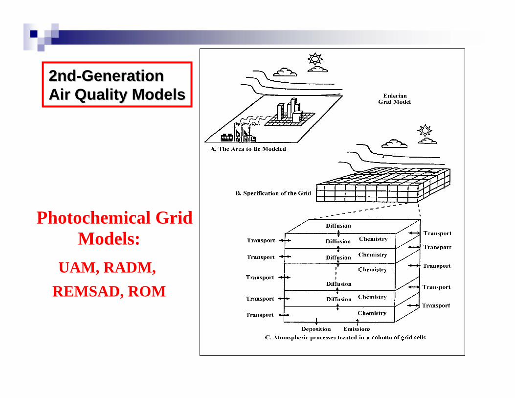
Photochemical Grid Models:
UAM, RADM, REMSAD, ROM
2nd2nd--Generation Generation Air Quality ModelsAir Quality Models

“One-Atmosphere” Modeling Multi-pollutant: Ozone, PM, visibility, acid and nutrients deposition, air toxics, etc.Multi-scale: International, National, Regional, Local
Advanced Computer Technologies Fast runtime (highly efficient for parallel & distributed computing) and cross-platform portability (supercomputers to PCs)
Examples include CAMx and EPA’s Community Multi-scale Air Quality (CMAQ) model
CMAQ code and documentation available from(http://www.cmascenter.org/)
Third-Generation Air Quality Models

Air Toxics
PM
Acid Rain
Visibility
Ozone
One-Atmosphere ApproachMobile Mobile SourcesSources
Industrial Industrial SourcesSources
Area Area SourcesSources
(Cars, trucks, planes,boats, etc.)
(Power plants, refineries/chemical plants, etc.)
(Residential, farmingcommercial, biogenic, etc.)
NOx, VOC,NOx, VOC,PM, ToxicsPM, Toxics
NOx, VOC, NOx, VOC, SOx, PM,SOx, PM,ToxicsToxics
NOx, VOC,NOx, VOC,PM, ToxicsPM, Toxics
Chemistry
Meteorology
Atmospheric DepositionClimate Change

Linkage betweenO3 and Fine PM
·O H
O 3
HO NO
V O C
Radical PoolHO 2·; RO 2·
C arbonyls
NO
H N O 3
FP
NO 2
S O x
H 2S O 4
N H 3
H O O H
hv
hv
C O
hv
SO x
C louds/Aqueous
orgaer
S ource
Secondary
S ink
PAN N2O 5
Nighttim e N 2O 5
·NO 3
C hem istry
H O2
hv
O1D
O3P
hv
N H 4N O 3
(Courtesy of Rich Sheffe, USEPA/OAQPS)
Fine PM Formation
Ozone Formation

MeteorologyProcessor
EmissionProcessor
Air QualityModel
SMOKE
Meteorological Data
Emissions Data
Air Quality Management Output
Ambient Data
Air Quality Modeling SystemAir Quality Modeling System

How do we use air quality models?

Why conduct Air Quality Modeling?Legal and Adminstrative Requirements
Clean Air Act and Amendments: Can serve as basis or legal justification for Agency action, e.g., OTAQ rules, NOx SIP Call, and CAIR.EO 12866 - Regulatory Planning and Review: Provide critical inputs to conduct benefits assessment for ‘major’ rules
Inform Policy Development & ImplementationNAAQS RIAs: Provides input to identification of “cost-effective” control measures for illustrative demonstration of achieving revised standard(s)Provide estimates of contributions to air quality concerns, e.g., CAIR, designations, and future multi-pollutant sector workState Implementation Plans (SIPs): Demonstrate attainment of NAAQS based on controls to be implemented by state/local agencies
Communication and OutreachProvides answers to the questions of stakeholders and the public about effectiveness and impacts of actions, e.g., future projections of nonattainment and attainment with regulation.

“Relative Use” of Air Quality ModelsWe use model estimates in a “relative” sense
Premise: models are better at predicting relative changes in concentrations than absolute concentrations
Relative Response Factors (RRF) are calculated by taking the ratio of the model’s future to current predictions of ozone or PM2.5 species
RRFs are calculated for ozone and for each component of PM2.5 and regional hazeTherefore, Future DV = Current DV times RRF
Projected ozone and PM2.5 concentrations are, thereby, “tied” to ambient measurements that provides a more robust and scientifically credible future projection of air quality.

Contribution of SO2 & NOx Emissions in Ohio to Annual Avg PM2.5- Based on Zero-Out Modeling for CAIR -

Maximum Contribution (ug/m3) to PM2.5 Nonattainment in Other States- Based on CAIR State-by-State Contribution Modeling -
0.980.19
CT: < 0.05NJ/DE: 0.21
MA: 0.07
MD/DC: 0.69
FL: 0.45
0.40
0.31
0.44
0.28
1.07
0.62
1.27
0.25
0.23
0.65
0.34
0.89
1.02 0.91 1.67
0.21
RI: < 0.05
0.90
0.56
0.84
0.29
0.12
0.11
0.07
< 0.05
0.11ME: < 0.05NH: < 0.05
VT: < 0.05
States Covered byCAIR for PM2.5

Elements of a Benefits Analysis
Estimate Expected Changes in Human Health Outcomes (Health
Impact Analysis)
Establish Baseline Conditions (Emissions, Air Quality, Health)
Estimate Expected Reductions in Pollutant Emissions
Model Changes in Ambient Concentrations of Ozone and PM
Estimate Expected Changes in Human Health Outcomes (Health
Impact Analysis)
Estimate Monetary Value of Changes in Health Impacts
Estimate Monetary Value of Health Impacts
Role of Air Quality Models

Role of Air Quality Models in Benefits Assessment
g ( )
Numberof
Counties
176
31
15
8
4
Legend<= 14.04 ug/m3
14.05 - 15.04 ug/m3
15.05 - 16.04 ug/m3
16.05 - 17.04 ug/m3
>= 17.05 ug/m3
Emissions, Costs, and Other Impacts (IPM)
Power Sector Emissions of Sulfur Dioxide
Air Quality Projections (CMAQ & CAMx)
Remaining Nonattainment Areas
Environmental Benefits
Visibility Improvement
Note: These maps are for illustrative purposes only and do not represent modeling results for any particular proposal.

Areas Designated as Nonattainment for 8-Hour Ozone and/or PM2.5
LegendBoth PM and Ozone NonattainmentPM Only NonattainmentOzone Only Nonattainment
Area Count
363
90

Remaining Areas Projected to Exceed the PM2.5 and 8-Hour Ozone Standards in 2020 with Future Baseline Emissions Absent Additional Regional or Local Controls
Area Count
7304
88
LegendBoth PM and Ozone NonattainmentPM Only NonattainmentOzone Only NonattainmentNonattainment areas projected to attain Source: 2005 Multi-pollutant Legislative Assessment

Remaining Areas Projected to Exceed the PM2.5 and 8-Hour Ozone Standards in 2020 with CAIR-CAMR-CAVR Absent Additional Local Controls
Area Count
3137
106
LegendBoth PM and Ozone NonattainmentPM Only NonattainmentOzone Only NonattainmentNonattainment areas projected to attain Source: 2005 Multi-pollutant Legislative Assessment

Air Quality Modeling Techniques:Contribution & Control Assessments
Address source/pollutant “contribution” to air quality concern
Sector Zero-Out ModelingModel simulation with “zero-out” of single or all pollutants from sector/sources of interest
Modeling Source ApportionmentAllows estimation of contributions from different source areas / categories within a single run
Address relative efficacy of source/pollutant emissions reductions
Response Surface Modeling (among others)A statistical “reduced-form” model of a complex air quality modelUsed in PM NAAQS for control strategy development as part of illustrative attainment of revised standards

Annual Average Contribution to Sulfate: Pulp and Paper Example
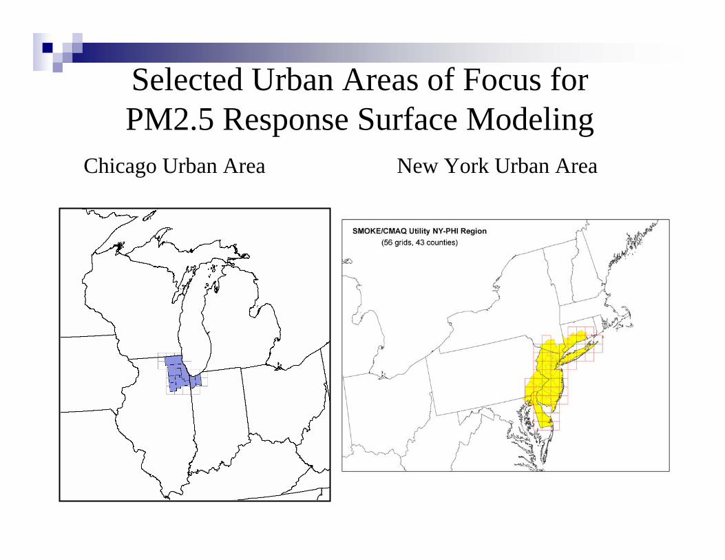
Chicago Urban Area New York Urban Area
Selected Urban Areas of Focus for PM2.5 Response Surface Modeling

Relative Effectiveness Per Ton of "Local" Emission Reductions Across Sources and Precursor Pollutants
Cook, IL New York, NY
"Local" EGU NOx
"Local" NonEGU NOx
"Local" Mobile NOx
"Local" EGU SO2
"Local" NonEGU SO2
"Local" Area SO2
"Local" VOC
"Local" Area NH3
"Local" Mobile NH3
"Local" Point Source POC & PEC
"Local" Mobile POC & PEC
"Local" Area POC & PEC
Relative effectiveness per ton in reducing ambient PM2.5 levels is only one factor in determining the appropriateness of controls. Cost effectiveness per microgram is the more complete measure, and reflects both the atmospheric response and costs of the controls.

What is a modeling platform?

What is a “Modeling Platform”?Structured system of connected modeling-related tools and data that provide a consistent and transparent basis for assessing the air quality response to changes in emissions and/or meteorologyCurrently, there are really two platforms
Regulatory Platform: CAPs-only with CMAQ used for regulatory analyses/future year projectionsMulti-Pollutant Platform: CAPs + HAPs with CMAQ & AERMOD (local scale modeling for Detroit); no future projections for toxics
Ultimately, certain aspects of these two platforms may merge into a single platform

Benefits of Using 2002 Modeling PlatformProvide consistency, transparency, and efficient development of baselines for:
OAR regulatory assessmentsCMAQ evaluations & research efforts by ORDAccountability efforts across EPAPublic health & exposure assessments
Promote multi-pollutant assessmentsIntegrated inventory (criteria and air toxics)“One-atmosphere” CMAQ with AERMOD for selected urban areas
Provide data and example for others outside of EPA
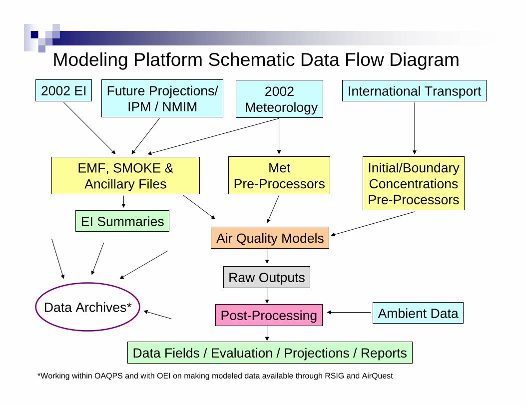
2002 EI 2002Meteorology
International Transport
Ambient Data
EMF, SMOKE &Ancillary Files
MetPre-Processors
Initial/BoundaryConcentrationsPre-Processors
Air Quality Models
Post-Processing
Data Fields / Evaluation / Projections / Reports
Future Projections/IPM / NMIM
Modeling Platform Schematic Data Flow Diagram
Raw Outputs
Data Archives*
EI Summaries
*Working within OAQPS and with OEI on making modeled data available through RSIG and AirQuest

Components of 2002 MP Modeling Platform2002 National Emissions Inventory (NEI)
Criteria and HAPs
2002 Meteorological DataMM-5 and MCIP v3.1Nationwide 36km Separate eastern and western 12km
Emissions Models, Tools and Ancillary DataEmissions Modeling Framework (EMF)SMOKE version 2.3.2, including BEIS3.13 and IPM 3.0Ancillary data updates
Emissions Projection MethodologyConsistent with approach developed for PM NAAQS
Air quality modelsCMAQ (v4.6.1i): nationwideAERMOD (promulgation version w/ dep): Detroit and “other” urban area

2002 National Emissions InventoryBest integration of CAPs and HAPs to dateElectric Generating Units (EGUs)
CEM data for SO2 and NOxOther pollutants use state or filled-in data
Mobile SourcesOn-road mobile from states or NMIM using MOBILE6Nonroad mobile from states or NMIM using NONROAD 2005Aircraft, Locomotive, and Marine from national totals subdividedto counties, and state data
NonEGU stationary point sources from state dataNonpoint (area) sources, including agricultural NH3 from animals and fertilizerWildfires and prescribed burning are (mostly) daily point-source based data

Projection Method Overview(CAPs only for now)
EGUs: Updated IPM modelStationary sources:
Known plant closuresNational program controls: NOX SIP, Consent Decrees & Settlements, MACT program, Wood Stove changeoutsRemoved spotty SIP info previously used in 2001 PlatformAnimal Population growth from DOA/SPPD to project emissions of NH3 from animals
Mobile:Latest VMT projections in collaboration with OTAQUse OTAQ’s NMIM to project onroad/nonroad and gas stage 2Info on loco/marine from OTAQ LTO growth for aircraftInformation from OTAQ on gas cans
Fires: Created new average fire sector

SMOKE Emissions Processing
Created SMOKE 2.3.2 specifically for platformAdvanced custom scripts and new approaches Ongoing performance improvements for this FYBiogenics from BEIS 3.13 with 2002 meteorologyEGUs: Hourly CEM data for SO2 and NOx(other pollutants follow hourly heat input)Ancillary data updates
SPECIATE4.1 speciation profiles via EMF’s Speciation ToolNew spatial surrogates vis EMF’s Surrogate ToolNew cross-references customized for CAP and CAP/HAP platforms


2002 Meteorological DataAnnual MM-5 Simulations
36 km US,12 km EUS,12 km WUS (from WRAP)Similar configuration as 2001 MM5 (but not identical)
MM5 data processed via MCIP v3.1 into CMAQModel evaluation indicated similar model performance as the 2001 MM5 simulations
Reasonable approximation of the actual meteorologyPrimary concern: 2-3 deg C underestimation of temperature in the winter months.Journal article fully summarizing evaluation findings will be available in 2008 (as part of CMAS).

Treatment of International Transport(Boundary Condition Concentrations)
GEOSChem – Global Chemistry Transport Model developed at Harvard Univ.
2002 simulations of GEOSChem provided via ICAP Domain covers entire globe: 2o x 2o grids and 30 layers up to the StratosphereProvides Boundary Conditions for CAPs and mercury and some other HAPS (e.g., formaldehyde) for our 36 km CONUS domain
For toxics not simulated by GEOSChem we used concentrations based on remote measurements and values in the literature via joint effort with AQAG and ORD

Community Multi-Scale Air Quality (CMAQ)
Photochemical grid model designed to simulate the formation and fate of ozone, oxidant precursors, primary and secondary particles, selected toxics, and deposition
Latest ‘interim’ version from ORD is v4.6.1i which includes scientific updates and advancements compared to earlier versions:
Integrated “one atmosphere” modeling capabilities including 38 toxic pollutants (see list at end of briefing); ORD plans to include this version in 2008 release of CMAQCarbon Bond 05 photochemical mechanism with mercury and chlorinechemistryAdded heterogeneous reaction involving nitrate and added sea saltImproved approach for treating convective mixing
Next official release will be CMAQ v4.8 with improved SOA mechanism among other improvements

Gas Phase HAPs in CMAQ v4.6.1iHAP CAS#
Acrylonitrile 107 -13-1Carbon Tetrachloride 56 -23 -5Propylene Dichloride 78 -87 -51,3-dichloropropene 542 -75-61,1,2,2 -Tetrachloride Ethane 79 -34 -5Benzene 71 -41 -2Chloroform 67 -66 -31,2 -Dibromomethane 106 -93-41,2 -Dichloromethane 107 -06-2Ethylene Oxide 75 -21 -8Methylene Chloride 75 -09 -2Perchloroethylene 127 -18-4Trichloroethylene 79 -01 -6Vinyl Chloride 7501 -4Naphthalene 91 -20 -3Quinoline 91 -22 -5Hydrazine 302 -01-22,4 -Toluene Diisocyanate 584 -84-9Hexamethylene 1,6 -Diisocyanate 822 -06-0Maleic Anhydride 108 -31-6Triethylamine 121 -44-81,4 -Dichlorobenzene 106 -46-7Total Formaldehyde 50 -00 -0Total Acetaldehyde 75 -07 -0Total Acrolein 107 -02-81, 3 -Butadiene 106 -99-0Formaldehyde Emissions Tracer 50 -00 -0Acetaldehyde Emissions Tracer 75 -07 -0Acrolein Emissions Tracer 107 -02-8
7647-01-0Hydrochloric acid
67-56-1methanol
7782-55-5chlorine
106-42-3p-xylene
108-38-3m-xylene
95-47-6o-xylene
108-88-3toluene
CAS#HAP
National or Regional Risk driver in NATA 1999

Aerosol Phase HAPs in CMAQ v4.6.1iHAP
Beryllium CompoundsNickel CompoundsChromium (III) CompoundsChromium (VI) CompoundsLead CompoundsManganese CompoundsCadmium CompoundsDiesel Emissions Tracer
Mercury
Multi-Phase HAPs in CMAQ v4.6.1i
National or Regional Risk driver in NATA 1999

AERMOD Modeling: DetroitAERMOD is an advanced steady-state plume dispersion model developed by AMS/EPA Regulatory Model Improvement Committee (AERMIC)
Current draft version will be usedIncludes dry and wet deposition algorithms based on work by ANLAllows multiple urban areas to be defined (will use Detroit MSA and Ann Arbor MSA)New option for varying emissions by hour-of-day and day-of-week (HRDOW7)
Link-based emissions based on AREA source algorithm with some comparisons to VOLUME source approach
2002 meteorological data derived from draft MM5-AERMOD Tool for Detroit

Key Modeling OutputsConcentrations of O3, PM2.5 species, mercury, and other toxics
Gridded fields used as inputs to BenMap for calculating health benefits of control strategies
Wet/dry deposition of sulfur, nitrogen (oxidized/reduced), mercury, and toxic species
Gridded fields used as inputs to Water/Eco models
Model evaluation and improvement in coordination with ORD
Projected O3 and PM2.5 design values by monitoring site; used for determining future attainment and residual nonattainment
Projected visibility at Improve sites in Class I Areas
CMAQ/AERMOD “Hybrid Approach” providing estimates of fine scale PM2.5 and toxics
O3 and PM2.5 are used as inputs to “data fusion” for CDC/Phase project

Highlights of 2002 Model Evaluation for CAPs[we can provide separate briefings with details]
OzoneUnder predicted for 1-hr and 8-hr daily max. especially O3 > 60 ppb
Similar to performance for 2001
Sulfate PM Under predicted (~up to 25%) for all seasons in the East and WestSimilar to performance for 2001
Sulfur DioxideOver predicted (~35 to >100%) in all seasons in the East and WestSimilar to performance for 2001
Nitrate PM Over predicted (~30 to > 100%) in the Fall, Winter, and in northern areas of the East in the SpringSignificantly different than performance for 2001

Organic PMOver predicted in the North and under predicted in South and West in the WinterUnder predicted in all areas (~25 to 65%) in Fall, Spring, and SummerSimilar to performance for 2001
Elemental CarbonMostly over predicted in urban areas (~45 to >100%) in all seasons in the East and WestMostly under predicted in rural areas (0 to >35%) in all seasons in the East and WestSimilar to performance for 2001
Highlights of 2002 Model Evaluation for CAPs
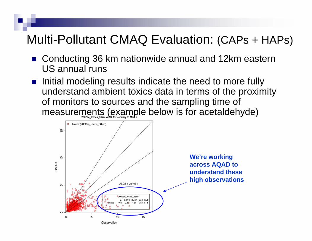
Multi-Pollutant CMAQ Evaluation: (CAPs + HAPs)
We’re working across AQAD to understand these high observations
Conducting 36 km nationwide annual and 12km eastern US annual runsInitial modeling results indicate the need to more fully understand ambient toxics data in terms of the proximity of monitors to sources and the sampling time of measurements (example below is for acetaldehyde)

Example of Multi-Pollutant Results- Spatial Characterization for July 8 -


How can this platform be used?

Near-Term Applications using the 2002-based Platform
O3 NAAQS Final RIAOTAQ rules and studies (Loco-Marine, Bond, SECA)Accountability/NOx responsivenessCDC/PHASEDetroit Multi-pollutant Pilot Study (CAPs+HAPs)Baltimore Health Indicators Study (CAPs+HAPs) (CDC/Region3/OAQPS/ORD)

Future Applications of PlatformOTAQ’s GHG ruleAdditional Climate ModelingNOx/SOx Secondary NAAQS
Risk Assessment and RIASector Modeling for SPPD
Includes source apportionment in CMAQ/CAMxPM2.5 Designations/Implementation RuleMulti-Pollutant Report (CAPs+HAPs)

Some “Non-traditional” Applications to Highlight
Detroit MP pilot studyEvaluate multi-pollutant platform in local area and inform OAQPS AQMP project & DEARS
DEARS and CDC/PHASEImprove air quality characterization for health studies and risk/exposure assessments
Climate ModelingExpand modeling platform to include climate feedbacks and interactions
Comprehensive Air Quality Management Plan:What are we doing for this project?
Partner with 4 states agencies to integrate the SIP requirements into a comprehensive AQMP
Assist on technical and policy issuesCompare outcomes with the traditional approach
3 pilot areas to develop a comprehensive planNew York – entire state (Region 2)North Carolina – entire state (Region 4)The entire state of Illinois combined with St. Louis, MO (Regions 5 and 7)

Implement Policy/Outreach Effort (AQPD/OID)Defined criteria and selected of partners for pilot studiesWill work with partners to identify issues to overcome and research potential incentives for areas to promote development of comprehensive AQMPs
Implement Technical Effort (AQAD/HEID/SPPD)Complete Detroit analytical work to provide valuable input and insights to selection of partners and design of pilot strategyWill provide template for analytical elements of pilot studies and technical input/consultation to partners as needed
Project elements: Two parallel efforts

Multi-pollutant Control Strategy /
SensitivityAnalysis
Exposures toHumans &
Environment
Multi-pollutant Control
Measures
Analytical Framework for Multi-pollutant Analysis
Assess Risk Reductions
& Co-benefits/Trade-offs
Integrated Emissions Inventory
Multi-pollutant Air QualityModeling
Modeling Platform

Multi-pollutant & Multi-scaleThe analytical framework emphasizes two main features:
(1) multi-pollutant (integration of HAPS & CAPS), and (2) multi-resolution (regional and local scales).
This provides a challenge for all analytical components:- Emissions Inventory: include HAPS & CAPS and support
regional and local scale modeling- Control Information: multi-pollutant for implementation into
control strategies or sensitivity analyses- AQ modeling: account for primary & secondary aspects of
criteria and toxic pollutants and assess regional and local concentrations and source contributions
- Exposure/risk/benefits assessment: provide information on benefit of pollutant reductions at regional and local scales forcriteria and toxic pollutants

Air Quality Modeling: “Hybrid approach”Allows preservation of the granular nature of AERMOD while properly treating chemistry/transport offered by CMAQ.
Generates local gradients incorporating the advantages of both the dispersion and photochemical models into one combined model output (via post-processing techniques)
AERMOD+CMAQCMAQAERMOD
CMAQ
AERMOD
Combined
AERMODAVG

Detroit Exposure and Aerosol Research Study (DEARS)
Describe the relationship between concentrations at a central site and residential/personal concentrations
PM constituents and Air ToxicsPM and Air Toxics from specific sources
Emphasis placed on understanding impact of:
Local sources (mobile and point) on outdoor residential concentrationsHousing type and house operation on indoor concentrationsLocations and activities on personal exposure

Exploration among US EPA and CDC, and 3 CDC State Partners: Maine, New York, and Wisconsin
Provide enhanced, easily accessible air quality information for use in Environmental Health Tracking
Model association between air quality and public health, e.g. mortalityAllow US EPA to measure effectiveness of control programs
Demonstrate use of spatial prediction using combined sources of data for environmental public health tracking:
Ambient air monitoring data (PM2.5 and O3) Air quality numerical model outputSatellite data, e.g. MODIS aerosol optical depth
Public Health Air Surveillance Evaluation (PHASE)

Typical Solution: use kriging to interpolate air monitoring data, but
Monitoring data is spatially sparse, some areas have no monitorsUse of classical kriging techniques may introduce arbitrarily large prediction errors in these areas
New Solution: Consider Combined Prediction ApproachesOutcomes:
Better air quality input for modeling linkages to public health dataMore accurate delineation of pollution non-attainment areas
Issue: Cannot monitor at all locations, but want to know pollutioneverywhere
Improve Spatial Prediction with Combined Air Quality Data
What Does the Combined Approach Provide ?Monitoring Data and CMAQ model output can be used simultaneously to predict the pollutant surfaceDraw on strengths of each data source:
Give more weight to accurate monitoring data in monitored areasRely on model output in non-monitored areasModel underlying spatial and temporal dependence, and measurement errors of each source

Example spatial surfaces for O3

Future Climate Modeling
Increased Temperature
O3 and PM2.5
Precipitation Changes
Cloud Cover Changes
Relative Humidity
Changes to…

Source Characterization
Greenhouse Gas Emissions
Control technologies
(CoST)
Global/Regional Climate Change
ModelingPrecursor Emissions
(NEI) Changes in Climate-Sensitive
Emissions
Changes in Ecosystem and
Human Sensitivity to air quality exposures
Regional Air Quality Modeling
CMAQ
Effects Modeling
Human Health
(BenMAP)Ecological
Other welfare
Climate Regulation Impact Assessment Framework
Changes in GHG Emissions
Changes in pollutant
concentrations/deposition
Changes in Precursor Emissions
Changes in
Interna
tiona
l Transp
ort
Changes in
Meteo
rolog
y
Changes in Meteorology

Ozone (8-hr max summer avg.)w/ 2001 Emissions & Current Climate
Summer 2000
Ensemble (2000-2002)Summer 2002
Summer 2001

2020 Base Emissions w/Current Climate
2020 CAIR Emissionsw/ Current Climate
2020 Base Emissions w/ Future Climate
2020 CAIR Emissions w/ Future Climate
Ozone (8-hr max summer avg., 3-yr ensemble) w/ 2020 Base & CAIR Control Emissions

Thank you for your time and patience!
Questions?