Multi-model ensembles for ecosystem

prediction

Michael A. Spence1,2,3*, Julia L. Blanchard4, Axel G. Rossberg5, Michael

R. Heath6, Johanna J Heymans7, Steven Mackinson3,8, Natalia Serpetti7,

Douglas Speirs6, Robert B. Thorpe3 and Paul G. Blackwell1

1School of Mathematics and Statistics, University of Sheffield, Sheffield,

UK2Department of Animal and Plant Sciences, University of Sheffield,

Sheffield, UK3Centre for Environment, Fisheries and Aquaculture Science, Lowestoft,

Suffolk NR33 0HT, UK4Institute for Marine and Antarctic Studies and Centre for Marine

Socioecology, University of Tasmania, 20 Castray Esplanade, Battery

Point. TAS. 70045Aquatic Ecology Group, Department of Organismal Biology, School of

Biological and Chemical Sciences, Queen Mary University of London,

Mile End Road, London E1 4NS6Department of Mathematics and Statistics, University of Strathclyde,

Glasgow G1 1XH, Scotland7Scottish Association for Marine Science, Scottish Marine Institute,

Oban, Argyll, PA371QA8Scottish Pelagic Fishermen’s Association, Heritage House, 135 - 139

Shore Street, Fraserburgh, Aberdeenshire, AB43 9BP*Corresponding author: michael.spence@cefas.co.uk

Abstract

When making predictions about ecosystems, we often have available a num-

ber of different ecosystem models that attempt to represent their dynamics in a

detailed mechanistic way. Each of these can be used as simulators of large-scale

experiments and make forecasts about the fate of ecosystems under different sce-

narios in order to support the development of appropriate management strategies.

1

arX

iv:1

709.

0518

9v1

[q-

bio.

QM

] 1

5 Se

p 20

17

However, structural differences, systematic discrepancies and uncertainties lead to

different models giving different predictions under these scenarios. This is further

complicated by the fact that the models may not be run with the same species or

functional groups, spatial structure or time scale. Rather than simply trying to

select a ‘best’ model, or taking some weighted average, it is important to exploit

the strengths of each of the available models, while learning from the differences

between them. To achieve this, we construct a flexible statistical model of the rela-

tionships between a collection or ‘ensemble’ of mechanistic models and their biases,

allowing for structural and parameter uncertainty and for different ways of rep-

resenting reality. Using this statistical meta-model, we can combine prior beliefs,

model estimates and direct observations using Bayesian methods, and make coher-

ent predictions of future outcomes under different scenarios with robust measures of

uncertainty. In this paper we present the modelling framework and discuss results

obtained using a diverse ensemble of models in scenarios involving future changes

in fishing levels. These examples illustrate the value of our approach in predicting

outcomes for possible strategies pertaining to climate and fisheries policy aimed at

improving food security and maintaining ecosystem integrity.

2

1 Introduction

Throughout ecology, ecosystem models are being used to support policy decisions

(Hyder et al 2015; Williams and Hooten 2016). Any such model is imperfect, and in

order to use it to inform policy making, it is important to quantify the uncertainty

of its predictions in a robust manner (Harwood and Stokes 2003). In many real

situations, there are several models available which each embody some knowledge

of a given ecosystem, however, they often differ in their predictions. Our aim here

is to describe and demonstrate a framework for using information from multiple

models in a coherent way that, following Chandler (2013), exploits their strengths

and discounts their weaknesses. Our approach involves statistical modelling of the

relationship between an ‘ensemble’ of ecosystem models. To avoid ambiguity we

will refer to the latter henceforth as ‘simulators’. We refer to the way in which a

simulator output differs from reality as its discrepancy.

Our statistical modelling will apply Bayesian inference methods (Robert 2007),

and our analysis will take into account any relevant prior knowledge as well as

simulator outputs that predict what would happen in the future under different

management scenarios. The Bayesian approach is subjective; for an introduction

to subjective uncertainty and decision theory, see Berger (1985). Strictly speaking,

any fully Bayesian analysis involves obtaining the posterior beliefs of a particular

individual, by combining their prior beliefs with information from data and mod-

elling. Depending on the context, that individual may be, for example, either a

scientist or a policy maker. Our framework includes the elicitation of prior beliefs

to combine with information from the model ensemble, allowing different individ-

uals’ posterior distributions to be obtained. For the purpose of our examples, the

individual chosen in each case is one of the authors.

We first review other approaches to ensemble modelling that can be taken. One

is to use a ‘democracy’ of simulators (Payne et al 2015; Knutti 2010), where each

simulator gets one vote, regardless of how well it represents the true system, and

a distribution of possible outputs comes from this. Similarly one could take an

average of the simulator outputs, which often outperforms all of the simulators

(Rougier 2016).

However, some simulators are better at predicting some outputs better than

others. An alternative approach is to try and find the “best” simulator(s) (Payne

et al 2015; Johnson and Omland 2004). These methods imply that at least one of

the simulators is “correct”, in the sense that it is able to predict the true output.

Not only is this a bold assumption, the addition of another simulator may allow

an area of the output space to become probable when before it was not. Thus by

increasing the number of models there is no guarantee that the uncertainty will

reduce.

One way of deciding which simulator is the “best” is to weight simulators using

Bayes factors, also known as Bayesian model averaging (Banner and Higgs 2017;

Ianelli et al 2016). However, this approach depends on the likelihood of the observa-

tions given a particular simulator, so if the simulators have been fitted to different

data, which is often the case in ecosystem simulators, computing Bayes factors is

impossible and more ad-hoc methods are then required (Ianelli et al 2016). This

could be further complicated as ecosystem simulators often work on different scales,

3

giving outputs that are not directly comparable to one another.

As Chandler (2013) explains, there is generally no simulator better in all respects

than the others and so there is no natural way of assigning a single weight to each

simulator. Furthermore if simulator outputs are not presented with uncertainty

then, in the case where the truth is a continuous quantity, a simulator will almost

never be “correct”, thus the probability of getting the true value from the ensemble

model is zero.

Climate scientists have moved away from simulator democracies and towards a

more general way of weighting the simulators in an effort to keep the good parts

of simulators and eliminate the bad (Knutti 2010). This leads to thinking of the

outputs from a simulator as being independently sampled from a population cen-

tred on the true value (Tebaldi et al 2005). In practice, there is no guarantee that

the population of simulators will centre on reality and as a result simulators share

biases and structural uncertainties (Knutti 2010). Furthermore, biases and discrep-

ancies will not be independent for all simulators, as researchers who build climate

simulators often contribute to a number of simulators either by developing them

directly or sharing ideas with their developers. The same applies in ecology, where

research groups could produce a number of ecosystem simulators, e.g. StrathE2E

(Heath 2012) and FishSUMs (Speirs et al 2010) from University of Strathclyde, or

could have similar inputs such as those coming from other simulators (e.g. Euro-

pean Regional Seas Ecosystem Model (Butenschon et al 2016)). When building

an ensemble model it is important to take these similarities into account rather

than treating the simulators as independent (Rougier et al 2013). This has led to

a number of ensemble models that treated the simulator outputs as coming from

a population and explicitly modelling the difference between the consensus of the

simulators and the truth (Tebaldi and Sanso 2009; Chandler 2013), known as the

shared discrepancy.

A key assumption in these statistical models is that all the simulators repre-

sent the same dynamical process and therefore the outputs should have similar

statistical structure (Leith and Chandler 2010). This is not necessarily going to be

the case with ecosystem models, as often their outputs are on different scales or

represent different dynamical processes, which are sometimes integrated out. Fur-

thermore these dynamics are generally less well understood than in climate science.

A further difficulty in applying these methods to ecosystem simulators is that the

simulators themselves have different outputs. For example in marine ecosystems,

the StrathE2E simulator (Heath 2012) models groups of species whereas the mizer

simulator (Blanchard et al 2014) models major species individually, the rest of the

ecosystem being included by an implicit background resources term (see appendix

C for an introduction to the simulators). It makes sense that these simulators

would, in an ensemble model, inform one another. For example if the StrathE2E

simulator implies that the mizer simulator overestimates demersal species in gen-

eral, then that suggests it is overestimating cod (Gadus morhua) in particular and

so StrathE2E is telling us something about cod indirectly. Using this idea, a hier-

archical structure for modelling the simulators allows us to sample the unobserved

outputs, conditional on the simulators’ observed outputs.

In this paper we describe an ensemble model which is based on the principles

of Chandler (2013) but which models the outputs themselves, varying in form be-

4

tween simulators, rather than statistical descriptors of the outputs. In Section 2

we examine a simple example of ensemble modelling by looking at the recovery

times of several marine indicators. In Section 3 we setup a more general framework

that will let us look at more complex examples. In Section 4 we use the model to

look at a specific case study: what would have happened in the North Sea if we

had stopped fishing in 2013? We conclude by discussing wider applications of the

approach in Section 5.

2 Introductory example

We think of the available simulators as being sampled from some conceptual pop-

ulation of possible simulators. Our a priori beliefs about each one are the same;

we are treating them as unlabelled ‘black boxes’. More formally, we regard the

simulators as ‘exchangeable’; see Gelman et al (2013). We consider relaxing this

assumption in Section 5. This idea is formalised by using a hierarchical model (for

more information see Gelman et al (2013)) to represent the ensemble of simulators

here.

In order to demonstrate this we look at a simple example to see how long it

would take indicators of good environmental status (GES) to recover if fishing

was reduced (HM Government 2012). Five simulators were run to equilibrium

using fishing mortality rates representative of the period 1985-1999. The fishing

mortality was then reduced by 41%, which is the median reduction of 1985-1999

rates required to attain advised fishing mortality values, and the simulators run

for a further 100 years. The time until each indicator recovered, defined as twice

the time it took the indicator value to change halfway between the two equilibrium

results, was recorded.

The selected indicators were as follows:

• Seabirds and mammals biomass (B&M): the biomass of seabirds and mam-

mals.

• Large fish indicator (LFI): the proportion of fish biomass pertaining to fish

longer than 40cm.

• Typical length (TyL): The biomass-weighted geometric mean length of a fish.

• Fish population biomass trends (FPBT): Biomass of fish.

• Ratio of zooplankton to phytoplankton (Z:P): the ratio of biomasses of zoo-

plankton to phytoplankton.

• Zooplankton biomass (ZB): the biomass of zooplankton.

In this example, we do not have any direct observations of the true values of the

recovery times; thus we are interested in learning about the simulator consensus,

µ. The simulator outputs, ui, are shown in Table 1. We model the relationship on

the log scale, with log10 ui = Mixi. Mi is a ni×6 matrix where ni is the number of

indicators output by model i. If model i outputs the jth indicator, one of the rows

of Mi will have a 1 in the jth column and 0s in the other columns (Dominici et al

2000). xi is a vector of the “best guess” of the ith simulator including, as latent

5

variables, the indicators that simulator i does not explicitly predict. For example,

for StrathE2E,

Mi =

1 0 0 0 0 0

0 0 0 0 1 0

0 0 0 0 0 1

,

representing the fact that StrathE2E predicts the 1st, 5th and 6th indicators. The

xis are modelled as coming from a multivariate normal distribution centred on the

simulator consensus, µ, with covariance C,

xi ∼ N(µ, C).

Table 1: Predicted recovery times of UK GES indicatorsIndicators Recovery time (in years)

Ecopath FishSUMS mizer StrathE2E PDMM

B&M 73.4 n/a n/a 21.5 n/a

LFI 4.7 7.6 5.0 n/a 8.9

TyL 3.7 4.6 6.1 n/a 7.4

FPBT n/a n/a 0.5 n/a 4.1

Z:P 2.5 n/a n/a 3.4 1.6

ZB 2.7 n/a n/a 3.2 1.6

2.1 Covariance matrix

The covariance matrix C is not known, but we can learn about it from the data,

through the model for xi, and we also have relevant prior information regarding

the correlations. One might expect that some of the indicators are more related

than others; for example recovery times of the ratio of zooplankton to phytoplankton

and zooplankton biomass are likely to be closely related whereas the recovery times

of Seabirds and mammals biomass and the Large fish indicator may not. Given

the difficulty of formulating priors on covariance matrices, we separate C into the

diagonal matrix Σ giving the standard deviations and the correlation matrix P ,

with

C = ΣPΣ.

By applying the prior

p(P ) = 1P�0

n−1∏i=1

n∏j=i+1

Beta(ρij |aij , bij),

we are able to elicit experts’ beliefs on correlations. Here 1P�0 is an indicator

function that takes the value 1 if P is positive definite and 0 otherwise, ρij is the

element of P on the ith row and jth column and Beta(x|a, b) is the density of a

Beta(a, b) distribution evaluated at x. We also put independent scalar distributions

on the diagonal elements of Σ, σi defined below.

6

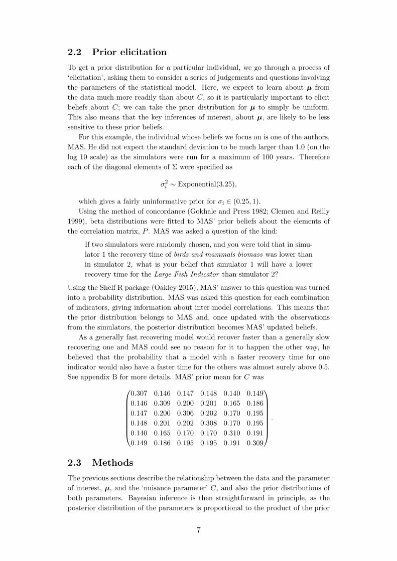
2.2 Prior elicitation

To get a prior distribution for a particular individual, we go through a process of

‘elicitation’, asking them to consider a series of judgements and questions involving

the parameters of the statistical model. Here, we expect to learn about µ from

the data much more readily than about C, so it is particularly important to elicit

beliefs about C; we can take the prior distribution for µ to simply be uniform.

This also means that the key inferences of interest, about µ, are likely to be less

sensitive to these prior beliefs.

For this example, the individual whose beliefs we focus on is one of the authors,

MAS. He did not expect the standard deviation to be much larger than 1.0 (on the

log 10 scale) as the simulators were run for a maximum of 100 years. Therefore

each of the diagonal elements of Σ were specified as

σ2i ∼ Exponential(3.25),

which gives a fairly uninformative prior for σi ∈ (0.25, 1).

Using the method of concordance (Gokhale and Press 1982; Clemen and Reilly

1999), beta distributions were fitted to MAS’ prior beliefs about the elements of

the correlation matrix, P . MAS was asked a question of the kind:

If two simulators were randomly chosen, and you were told that in simu-

lator 1 the recovery time of birds and mammals biomass was lower than

in simulator 2, what is your belief that simulator 1 will have a lower

recovery time for the Large Fish Indicator than simulator 2?

Using the Shelf R package (Oakley 2015), MAS’ answer to this question was turned

into a probability distribution. MAS was asked this question for each combination

of indicators, giving information about inter-model correlations. This means that

the prior distribution belongs to MAS and, once updated with the observations

from the simulators, the posterior distribution becomes MAS’ updated beliefs.

As a generally fast recovering model would recover faster than a generally slow

recovering one and MAS could see no reason for it to happen the other way, he

believed that the probability that a model with a faster recovery time for one

indicator would also have a faster time for the others was almost surely above 0.5.

See appendix B for more details. MAS’ prior mean for C was

0.307 0.146 0.147 0.148 0.140 0.149

0.146 0.309 0.200 0.201 0.165 0.186

0.147 0.200 0.306 0.202 0.170 0.195

0.148 0.201 0.202 0.308 0.170 0.195

0.140 0.165 0.170 0.170 0.310 0.191

0.149 0.186 0.195 0.195 0.191 0.309

.

2.3 Methods

The previous sections describe the relationship between the data and the parameter

of interest, µ, and the ‘nuisance parameter’ C, and also the prior distributions of

both parameters. Bayesian inference is then straightforward in principle, as the

posterior distribution of the parameters is proportional to the product of the prior

7

and the likelihood. In practice, the calculation of the posterior is not mathemati-

cally tractable, so we take the well established approach of using a simulation-based

algorithm to sample from the posterior distribution. Because of the dimensionality

and correlation of the uncertain parameter space, we fitted the model using No

U-turn Hamiltonian Monte Carlo (Hoffman and Gelman 2011) in the package Stan

(Gelman et al 2015).

2.4 Results

Ye

ars

0.0

10

.11

10

10

01

00

0

Birds an

d m

amm

als biom

ass

Larg

e Fis

h In

dica

tor

Typica

l len

gth

Fish

popu

latio

n biom

ass

Biom

ass ra

tio Z

:P

Zooplan

kton

biom

ass

Figure 1: The marginal posterior distributions of the simulator consensus, µ, for the

recovery times of each of the indicators.

Figure 1 shows the marginal posterior distributions of the elements of the sim-

ulator consensus, µ, of the recovery times. These represent the logically updated

beliefs of MAS after learning from the observed simulator runs. MAS is more un-

certain about the recovery times of the birds and mammals biomass and the fish

population biomass. This is because only two of the simulators model each of

these. He is much more certain about the LFI and Typical length, each of which

was predicted by four simulators.

Despite this uncertainty, MAS has probability 0.84 that all of the indicators,

8

except Birds and mammals biomass, will recover within 10 years and 0.19 of recov-

ering within five.

3 General framework

In the example in the previous section we inferred the simulator consensus, µ.

However, there is no reason to believe that this will be the truth (Chandler 2013)

so we need to allow some difference between the model consensus and truth, the

shared discrepancy.

To illustrate these ideas, we start by sketching out a toy example, much simpler

than our actual case study. We are interested in n true quantities, y = (y1, . . . , yn),

e.g. biomasses of n species at a particular time. We have m simulators, each giv-

ing an output representing the quantities of interest, xi = (xi1, . . . , xin) for i =

1, . . . ,m. We also have noisy observations of the truthw = (w1, . . . , wn). We regard

the simulators as coming from a population with mean output µ = (µ1, . . . , µn),

known as the simulator consensus. To define our ensemble model, we then model

separately the relationships between the noisy observations and the truth, the dif-

ference between y and µ (that is, the shared discrepancy) and the distribution of

the simulator outputs around µ. Figure 2 represents the ensemble model in the

form of a directed acyclic graph (DAG) (Lunn et al 2012), where the arrows show

the direct dependencies between variables.

w

y

µ

· · ·x1 xm

Figure 2: The directed acyclic graph of the toy example.

For a realistic example, there are a number of additional factors to consider.

We need to distinguish between an idealised version of simulator i, using the best

possible parameters and inputs to produce outputs xi, and the available version of

it with uncertain parameters producing outputs ui. This is important since we may

well have information about the likely difference between xi and ui, for example

as a consequence of parameter estimation. Furthermore, the differences between

the simulators mean that some elements of ui may be unobserved for particular

models. Finally, we are generally interested in the dynamics of the ecosystem,

9

either for its own sake or because we are interested in future states; thus all of the

above quantities are also indexed by time. Again, not all of them will actually be

observed at all times; obviously we have no data corresponding directly to future

times. However, in formulating the model, we retain all the corresponding variables;

in particular, our aim typically is to learn about the unobserved future true values.

Extending the notation to allow for these generalisations, we let y(t) be a vector

of length n of the truth at time t for t = 1 . . . T , where T is the length of the

whole simulation, u(t)i be a vector of length ni that represents the actual observed

simulator outputs for i = 1 . . .m, the number of simulators, and t ∈ Si, the set

of times at which simulator i gives outputs and w(t) be a vector of length ny that

represents noisy observations of the truth for t ∈ S0, the set of times at which there

are observations. Let x(t)i be the unknown output from the idealised version of

simulator i, our estimate of this will be our “best guess” of the output for simulator

i at time t where t = 1 . . . T , and let µ(t) be the simulator consensus at time t. We

are interested in the future values of y(1:T ) conditional on all of the information we

have received,

p(y(1:T )|w(S0:T0),u(S1:T1)1 , . . . ,u

(SM :TM )M ). (1)

The ensemble model follows the hierarchical structure shown by the directed acyclic

graph (DAG) in Figure 3. Conditional on y(t), w(t) and w(t+1) are independent

w(t)

y(t)

µ(t)

· · ·x(t)1 x

(t)m

u(t)1 u

(t)m

w(t+1)

y(t+1)

µ(t+1)

· · ·x(t+1)1 x

(t+1)m

u(t+1)1 u

(t+1)m

Figure 3: The directed acyclic graph of the ensemble model.

of one another. Similarly, conditional on x(t)i , u

(t)i and u

(t+1)i are independent of

one another. The truth, y(t), the model consensus, µ(t), and the simulators’ “best

guesses”, x(t)i , do depend on their values at the previous time step. The ensemble

model as a whole is a Markov process such that conditional on the present, the past

and the future are independent of one another.

10

Direct calculation of the distribution in equation 1 is impossible except in the

very simplest cases. In general, we use simulation-based methods such as Markov

chain Monte Carlo (MCMC) to sample from

p(y(1:T ),µ(1:T ),x(1:T )1 , . . . ,x

(1:T )M |w(S0:T0),u

(S1:T1)1 , . . . ,u

(SM :TM )M )

and hence from the distribution of interest. Using mathematical simplifications

based on the conditional independence structure in the DAG in Figure 3 (see Ap-

pendix A), this approach can be implemented in standard software such as BUGS

(Lunn et al 2012), JAGS (Plummer 2003) or Stan (Gelman et al 2015), using the

details of each component of the model, which are given in Sections 3.1 to 3.4.

3.1 The truth

In the absence of any simulators, our prior beliefs for the truth at time t, y(t) follows

a random walk,

y(t) = y(t−1) + εΛ,t, (2)

where each εΛ,t is centred on 0 with covariance Λy. At time point t0, the truth,

y(t0), follows a generic prior distribution p(y(t0)).

3.2 Direct observation

At times t ∈ S0, there are noisy and possibly indirect observations of the truth,

w(t), which come from some distribution, p(w(t)|y(t)) that is problem specific and

is caused by data uncertainty (Li and Wu 2006). The elements of w(t) may not be

the same as that of y(t), for example if observations are incomplete or aggregated,

we assume that the sampling distribution of observations depends on the truth

through some function fy(·) such that

w(t) = fy(y(t))

and

p(w(t)|y(t)) = p(w(t)|w(t)).

For example if w(t) is some linear transformation of y(t), then

w(t) = Myy(t)

where My is an ny × n matrix, with ny ≤ n in practice.

3.3 Model of the simulators

The difference between the simulator consensus, µ(t), and simulator i’s “best guess”,

x(t)i , is simulator i’s individual discrepancy, z

(t)i , where

z(t)i + γi = x

(t)i − µ

(t).

This distinguishes the individual discrepancy between the long-term discrepancy,

γi = εγ,i,

11

where εγ,i is an n dimensional random variable centred on 0 with covariance C,

and the short term discrepancy z(t)i . It seems natural to allow z

(t)i and z

(t+1)i to

be dependent on each other; for example, if at time t, z(t)i was less than 0, then

z(t+1)i might also be expected to be less than 0. With this in mind, we say that

z(t)i follows a stationary auto-regressive model of order 1,

z(t)i = Riz

(t−1)i + εz,t,i, (3)

where each εz,t is an independent n-dimensional random variable centred on 0 with

covariance Λi and Ri is an n×n matrix with the constraint such that Ri is stable, i.e.

limn→∞Rni = 0. Ri and Λi describe the dynamics of simulator i with Ri ∼ gR(θ)

and Λi ∼ gΛ(φ) for some distributions gR and gΛ with hyperparameters θ and φ

respectively. At time t0, z(t0)i is sampled from it’s stationary distribution with mean

0 and covariance Γi, such that

vec(Γi) = (I −Ri ⊗Ri)−1vec(Λi)

where vec is the vectorization operator representing the ‘stacking’ of the columns

of a matrix, and ⊗ denotes the Kronecker product of matrices.

3.4 Uncertainty in simulator outputs

The simulators’ outputs, u(t)i , are noisy, possibly indirect, observations of the sim-

ulators’ “best guess”, x(t)i for t ∈ Si. The distribution of u

(t)i is the posterior

predictive distribution for simulator i. Furthermore, u(t)i does not necessarily con-

tain all of the elements of x(t)i . Similar to the observations of the truth, simulator

i’s “best guess” for the elements of u(t)i is

u(t)i = fi(x

(t)i ),

and therefore u(t)i ∼ p(u

(t)i |u

(t)i ). In practice

u(t)i = Mix

(t)i

is a common form. Each simulator is fitted to a finite set of data, Di, in order to

find p(u(t)i |Di), from which u

(t)i is sampled.

3.5 Linking the simulators and the truth

The shared discrepancy, the difference between the simulator consensus, µ(t), and

truth, y(t), is split up into the long-term shared discrepancy, δ, and the short-term

discrepancy, η(t), i.e.

δ + η(t) = y(t) − µ(t).

The short-term discrepancy is modelled with a stationary auto-regressive model of

order 1

η(t) = Rηη(t−1) + εη,t,

12

Table 2: A summary of the variables in the ensemble model. The ensemble model is run

from time 0 up until time T .Variable time period Name

y(t) t = 0 . . . T The truth

w(t) t = 0 . . . T Possibly incomplete observation of truth

w(t) t ∈ S0 Noisy observation of w(t)

δ NA Long-term shared discrepancy

η(t) t = 0 . . . T Short-term shared discrepancy

µ(t) t = 0 . . . T Simulator concensus

γi NA Simulator i’s long-term individual discrepancy

z(t)i t = 0 . . . T Simulator i’s short-term individual discrepancy

x(t)i t = 0 . . . T Simulator i’s best guess

u(t)i t = 0 . . . T Simulator i’s incomplete observation of x

(t)i

u(t)i t ∈ Si Simulator i’s output

where Rη is stable and εη,t is an n dimensional random variable centred on 0 with

covariance ∆. At time t0, η(t0) is sampled from its stationary distribution with

mean 0 and covariance Γη, such that

vec(Γη) = (I −Rη ⊗Rη)−1vec(∆).

Table 2 summarises the variables in the model.

4 Case Study

We illustrate our model by looking at a problem where a decision maker, who is

responsible and accountable for her actions, is to make judgements about what

would happen to the biomass of demersal species in the North Sea if fishing were to

stop completely in 2014, using outputs from 5 different ecosystem simulators and

International Bottom Trawl Survey (IBTS) data (ICES Database of Trawl Surveys

(DATRAS) 2015). In this example, one of the authors JLB, has taken the role as

the decision maker. Her prior beliefs are elicited and expressed as prior distributions

and then the posterior beliefs that we show belong to her.

4.1 Groups of species

The five simulators, detailed in Appendix C, represent demersal fish in different

ways, with different species resolution and coverage. While our main interest is

in demersal fish collectively, we need to represent the state of the ecosystem at a

resolution that enables us to link these simulator outputs together.

We thus group the species so that species that are represented in the same

way in exactly the same simulators are in the same group, and whenever one of

the simulators gives an output that is aggregated over multiple species, then that

output can be expressed as a sum of one or more of our groups. The groups

13

do not necessarily have any direct biological interpretation; provided the groups

meet the criteria above, and allow us to represent the quantities of interest—here,

demeral fish, given by the sum of all groups—the precise choice will not affect the

answer obtained. For computational efficiency, we choose the minimum number of

groups that meets these criteria while covering all demersal species. For example we

grouped together monkfish, long rough dab, lemon sole and witch because they all

occur in exactly the same simulators, as individual species in Ecopath and LeMans

and implicitly in StrathE2E, but are not contained in any larger set of species for

which this is true. This minimal set consists of 5 groups, which we will model

explicitly. The groups are:

1. Common demersal : These are cod (Gadus morhua), haddock (Melanogram-

mus aeglefinus), whiting (Merlangius merlangus), Norway pout (Trisopterus

esmarkii), plaice (Pleuronectes platessa), common dab (Limanda limanda)

and grey gurnard (Eutrigla gurnardus).

2. Sole (Solea solea).

3. Monkfish etc.: These are monkfish (Lophius piscatorius), long rough dab (Hip-

poglossoides platessoides), lemon sole (Microstomus kitt) and witch (Glypto-

cephalus cynoglossus).

4. Poor Cod and Rays: These are poor cod (Trisopterus minutus), starry rays

(Amblyraja radiata) and cuckoo rays (Leucoraja naevus).

5. Other demersal fish: This consists of all other demersal fish.

We consider the total biomass densities for each of these groups, in tonnes per

square kilometre, modelled on the log scale (to base 10, for ease of interpretation).

4.2 Data and elements of the statistical model

The IBTS data were extracted as in Fung et al (2012), to reveal the total catch

on the survey for each of the 5 groups for the first (1986-2013) and third quarter

(1991-2013). How this value relates to the true biomass density in the North Sea is

not trivial, and these values are often multiplied by catchability coefficients (Walker

et al 2017) which are themselves uncertain and model-based. In this example we

are only interested in the biomass density relative to 2010 and therefore the total

catch from the IBTS survey is enough as we assume that catchability coefficients

are constant over time. Thus each element of yt represents the log to base 10 of the

total biomass density for one of our groups of species, averaged over year t year,

relative to 2010. Therefore in the notation of Section 3.2,

w(t) = fy(y(t)) = y(t).

The measurement error on the observations of the truth is assumed to be normally

distributed on the log10 scale such that

w(t) −w(2010) ∼ N(y(t),Σy),

for t 6= 2010. In this work we take Σy to be 2 log10(1.15) on the diagonal elements

and 0 on the off diagonal elements. This was chosen so that it means that the

standard deviation of the true biomass would be 15% of the actual amount caught.

14

4.3 Simulators

We have outputs from 5 different simulators, all of which have been run with zero

fishing pressure from 2013 onwards. In the next few subsections we describe the

models that we used in the ensemble. The ith simulator’s output is assumed to be

normally distributed on the log10 scale,

u(t)i ∼ N(u

(t)i ,Σi),

with Σi fitted based on running simulator i many times (Leith and Chandler 2010;

Chandler 2013). However, if this was not the case Σi could be estimated within

the hierarchical system. The 5 simulators and their parameter uncertainty are

described in Appendix C.

4.4 Ensemble model

Each element of x(t)i is the “best guess” of simulator i of the elements of y(t), for

t = 1968, . . . , 2100, in log (base 10) tonnes per km of wet biomass. In this example

we expect each of the simulators to converge to its own steady state, given that

all external drivers are constant. This means that in equation 3 we expect Ri to

tend towards 1 and Λi to tend towards 0. Furthermore, if a simulator reaches a

stationary state before it has stopped running, then we know that it will be in that

state forever. Simulator i’s individual discrepancy, γi + z(t)i , is thus modelled as

γi ∼ N(0, C)

and

z(t)i ∼

{N(Riz

(t−1)i ,Λi) if < t ≤ 2013,

N(hz(Ri, ki, t)zt−1i , hΛ(t, ki)Λi) if 2014 ≤ t.

where

hz(Ri, k, t) = Ri + (1−Ri)(1− hΛ(t, ki))

and

hΛ(t, ki) = exp {−ki (t− 2013)} .

This is saying that, after the end of fishing, the variance of the truth of model i

reduces and the amount that the last value of z(t)i relates to the next moves towards

1 by a factor of exp(ki) each year. We take ki ∈ [0, 6], as there is not much difference

numerically if ki goes above 6, with

ki/6 ∼ Beta(ak, bk).

The diagonal elements of Ri fall between −1 and 1 with

Ri + 1

2∼ Beta(aR, bR)

and the off-diagonal elements are set to 0. The model-specific variance parameter,

Λi, is decomposed into a diagonal matrix of variances, Πi, and a correlation matrix,

Pi, such that

Λi = ΠiPiΠi.

15

The form of the prior distribution for the jth diagonal element of Πi was

πij ∼ Gamma(απ,j , βπ,j).

Distributions over correlation matrices are complicated by the mathematical re-

quirement of positive definiteness. In practice, we specify separate priors on the

elements, and then condition on positive definiteness; the unconditional prior for

the j, kth element of Pi is given by

ρijk + 1

2∼

{Beta(aρjk, bρjk) if j 6= k,

1 otherwise.

The difference between the truth at time t and the corresponding simulator con-

sensus, µ(t), is then (y(t))−(µ(t) − µ(2010)

)= η(t) + δ

with

η(t) ∼ N(Rηη(t−1),∆η). (4)

When the fishing is turned off, we are particularly uncertain about what will hap-

pen; thus we will remove any direct relation between yt and yt+1 beyond that time.

We will say that

µ(t) ∼ N(µ(t−1), hΛ(t, kµ)∆µ) (5)

where kµ ∈ [0, 6], so that the simulator consensus reaches a stationary point, as the

individual simulators do.

As in the introductory example, we focus on the subjective probabilities of

a particular individual, in this case JLB. Her prior beliefs were elicited using the

method described in O’Hagan et al (2006) and Alhussain and Oakley (2017). Details

of the prior elicitation can be found in Appendix D.

4.5 Results

Due to the dimensionality and correlation of the uncertain parameter space, we

fitted the model using No U-turn Hamiltonian Monte Carlo (Hoffman and Gelman

2011) in the package Stan (Gelman et al 2015).

Figure 4 shows the results for the relative biomass over time for each group of

species, if we had stopped fishing in 2013. In the notation above, that means that

each plot relates to the marginal posterior distributions of each element of y(t), for

all t. In each case, the solid line shows the posterior median output and the dotted

lines the upper and lower posterior quartiles of that output. The common demersal

fish increase which is unsurprising as this group contains a lot of species targeted

by fisheries and all of the individual simulators predict that.

The ensemble model and Bayesian statistical framework allow us to make proba-

bility statements, such as: the probability that there will be a greater total biomass

of common demersal in 2050 than in 2010 is 0.90. There is a similar number for

sole (0.93) and for monkfish etc. (0.88) but it its lower for poor cod and rays (0.55)

and for the other demersal species (0.17).

16

Common demersal

Year

Re

lative

bio

ma

ss

1970 1990 2010 2030 2050 2070 2090

0.9

11

.11

.2

Sole

Year

Re

lative

bio

ma

ss

1970 1990 2010 2030 2050 2070 2090

0.7

51

.52

.5Monkfish etc.

Year

Re

lative

bio

ma

ss

1970 1990 2010 2030 2050 2070 2090

0.5

11

.5

Poor cod and rays

Year

Re

lative

bio

ma

ss

1970 1990 2010 2030 2050 2070 2090

0.5

11

.52

.54

Other demersal

Year

Re

lative

bio

ma

ss

1970 1990 2010 2030 2050 2070 2090

0.5

12

3

Figure 4: Estimates of the log biomass of each group of species relative to 2010. The

solid line is the median and the dotted lines are the upper and lower quartiles. The first

vertical line is at 1986, the year that we first have data, and the second line is in 2013,

the year before fishing were to stop completely.

17

The ensemble model also ‘predicts’ what happened before the data; that is, it

gives posterior distributions for the actual values given the imperfect data and the

simulator runs. Only sole and common demersal are output by simulators prior to

1986 and this is reflected in the increased uncertainty as we move further back in

time from 1986.

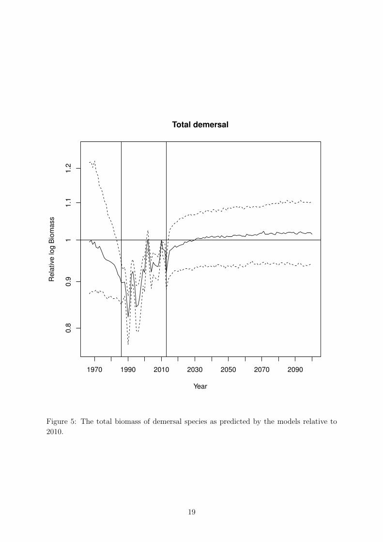
The total biomass of demersal species is difficult to calculate here because the

discrepancy between the simulator consensus and the truth is difficult to quantify.

We do not have direct survey data the we can use for true total demersal biomass;

values depend on the varying, and unknown, catchability coefficients for each of

the groups. Figure 5 shows the total demersal biomass if we assumed that the

groups had the same catchability coefficient. It shows that we are rather uncertain

about whether the biomass will grow relative to the biomass in 2010. However,

what it was before 1986 is quite uncertain. This is because of the uncertainty in

the populations of Other demersal species. We found that in 2050 the biomass will

be larger than in 2010 with probability 0.55.

The median “best guess” of each of the simulators is shown in Figure 6. Notice

that StrathE2E predicts quite a large increase in common demersal despite not

explicitly outputting it.

The posterior predictive distribution for the relative truth in 2025 for common

demersal and monkfish etc. is positively correlated (0.28). This suggest that learn-

ing something about the common demersal would tell you something about monk-

fish etc. Hence the mizer simulator gives some information regarding the monkfish

etc. despite not actually predicting it. See Appendix E for the other correlations

between the groups.

5 Discussion

By treating the simulator outputs as coming from a population of simulators and

modelling this population, we have presented in this paper a general way of com-

bining ecosystem simulators in order to inform a decision maker about the forecast

under a specific management strategy. Our model combines a number of different

simulators, exploiting their strengths and discounting their weaknesses (Chandler

2013) to best inform the decision maker.

5.1 Case study results

We demonstrated how to combine simulators with different outputs by predicting

how fast different indicators would recover if we were to reduce the fishing mor-

tality. We further demonstrated our model by using 5 ecosystem simulators and

investigating what would have happened to demersal fish in the North Sea if we

had stopped fishing in 2014. We found that although the total biomass of demersal

fish may not increase over time, the biomass of targeted fish will likely increase

relative to 2010.

18

Total demersal

Year

Rela

tive log B

iom

ass

1970 1990 2010 2030 2050 2070 2090

0.8

0.9

11.1

1.2

Figure 5: The total biomass of demersal species as predicted by the models relative to

2010.

19

Common demersal

Year

Bio

ma

ss t

on

ne

s p

er

km

sq

1970 1990 2010 2030 2050 2070 2090

51

02

0

Sole

YearB

iom

ass t

on

ne

s p

er

km

sq

1970 1990 2010 2030 2050 2070 2090

0.1

0.2

0.4

Monkfish etc.

Year

Bio

ma

ss t

on

ne

s p

er

km

sq

1970 1990 2010 2030 2050 2070 2090

0.2

50

.51

Poor cod and rays

Year

Bio

ma

ss t

on

ne

s p

er

km

sq

1970 1990 2010 2030 2050 2070 2090

0.5

12

4

Other demersal

Year

Bio

ma

ss t

on

ne

s p

er

km

sq

1970 1990 2010 2030 2050 2070 2090

0.0

25

0.1

0.4 Ecopath

MizerStrathE2EFishSUMsLeMansµ

Upper and lower quartiles of µ

Figure 6: The median best guess for the simulators (xi) for mizer (black), FishSUMS

(purple), LeMans (green), Ecopath (red) and StrathE2E (pink) and the median simulator

consensus (µ) and its quartiles in solid grey and dotted grey respectively.

20

5.2 General model features

One of the difficulties in building an ensemble model with ecosystem simulators

is that the simulators outputs are often done on different scales and are not di-

rectly comparable, for example StrathE2E models groups of species (e.g. pelagic,

demersal) whereas mizer models major species individually. Our approach, unlike

existing methods of combining simulators (e.g. Bayesian model averaging (Banner

and Higgs 2017; Ianelli et al 2016)), allows us to combine outputs from these widely

differing simulators. We achieve this by modelling what each simulator would pre-

dict for each of the groups of species we are interested in, whether it is explicitly

modelled or not by the simulator.

For example, in the case study, StrathE2E only models the total demersal

species. Using information from the other simulators regarding the breakdown of

demersal species and how the dynamics between species work, the ensemble model

is able to say what StrathE2E would predict on a species level.

Ecopath and StrathE2E both predict sums of things. For Ecopath it is the sum

of poor cod and rays and other demersal and StrathE2E gives the sums of all of

the groups. As with the simulators that do not predict specific species, we are able

to infer what these models predict about the things that they sum over though

correlations learned by other simulators. In this sense, the mizer model, which

only predicts common demersal and sole, gives information about how StrathE2E

divides its demersal species and therefore gives some information to other species.

Therefore, if we were interested in what would happen to the other demersals if

we were to stop fishing, we should include all of the simulators despite only two of

them predicting it.

The ensemble enables the uncertainty of the predictions to be quantified in

a robust manner. The uncertainty in the prediction increases the further away

from the observations of the truth both when forecasting and hindcasting. The

uncertainty increases when there are fewer simulators that give outputs. All of the

simulators give outputs for the common demersal, four explicitly and one implicitly,

and therefore we are more certain about what will happen in the future whereas

for poor cod and rays, where only three simulators predict values for the future

and only one explicitly, the uncertainty is much higher. The uncertainty is highest

for other demersal species. This is understandable as only two simulators predict

values for this group of species, neither of which does so explicitly.

The hierarchical distributions for the covariance parameter for the short-term

individual discrepancy, Λi, was divided into a diagonal matrix Πi, with the jth

diagonal element being the standard deviation of the jth element, and correlation

matrix Pi. It was divided this way, as there is more information about the dynamics

of species in models as opposed to the variance. In ecosystems simulators, the

dynamics are going to be similar in direction but maybe not in magnitude.

In the case study, we used beta distributions for each of the off diagonal ele-

ments of the correlation matrix and then conditioned on positive definiteness. This

enabled us to learn about each element of the correlation matrix separately which

is not possible in other formulations of the covariance matrix (Alvarez et al 2014).

It was also important to use informative priors as none of the simulators explicitly

model other demersal. As there is no lower bound (on the log scale) for the values

21

of the “best guess” of other demersal, we required some prior information about

the distribution of the standard deviations, Π. This does suggest that the ensemble

prediction is somewhat based on that of the priors for Λi. In practise we suggest

checking your ensemble model predicts in a way that the decision maker believes

before data observing the truth. In the case study described here that is prior to

1986, similar to the hypothetical data method of Kadane et al (1980).

When building the ensemble model, how the species groups are decided depends

on the question being asked. In the case study we were interested in what would

happen to demersal fish if we were to stop fishing, so we grouped the species into

as few groups as possible. However, if we were interested in another question, for

example if we had been interested in what would happen to commercial fish, we

would divide the species into groups with commercial and non-commercial fish con-

ditioned on species in each group being presented in exactly the same simulators.

As the number of groups increases, the dimensions of the covariance matrices in-

crease, so we advice that the number of groups be kept to a minimum as this would

aid computation time and require less simulators and prior elicitation.

Using the ensemble model developed here, there is no need to identify the “best

model” driven by the question being asked (Dickey-Collas et al 2014), but one

should include all available simulators. Rather than developing a number of sim-

ulation models to answer different specific questions, the ensemble model can be

designed to answer the question at hand. Furthermore, as the ensemble model

aims to exploit simulators strengths and discount their weaknesses, it is better for

a simulator to be really good at modelling one aspect of the ecosystem than being

okay at modelling a lot of things.

Due to the nature of the different ecosystem simulators, they often have different

processes and are often unable to run the same scenarios, for example the mizer

model doesn’t have climate dynamics included in it. If we are interested in one of

the scenarios that a specific simulator is unable to run we should still include that

simulator in the ensemble model as it gives information about how species interact

with one another as well as the state of the ecosystem up until the current time. In

order to include this simulator in the ensemble, we could increase Σi as a function

of time with in future scenarios. This would suggest mean that the simulators “best

guess”, which in this case means what the simulator would predict if it were able

to run the scenario, would be less informed by the simulator output as time went

on.

5.3 Future work and extensions

Some ecosystem simulators are more similar than others, for example there are

a number of size-based simulators in the marine literature (e.g. Blanchard et al

2009; Scott et al 2014) that are very similar, which may violate the exchangeability

assumption made in Section 3. Additional hierarchy could be added to the ensemble

model that would allow such simulators to have more similar discrepancies.

In climate science, where the simulators are very similar to one another and it is

possible to create a phylogenetic tree (Knutti et al 2013) that shows the development

history of each simulator, Demetriou (2016) did add additional hierarchy allowing

closely related simulators to have similar discrepancies. They found that the major

22

source of uncertainty was that of the shared discrepancy and that the results of the

ensemble model were very much similar to all of the simulators being exchangeable.

Additionally, if there were multiple observations, it is possible to include this

by adding a number of observations of the real system y. This could be important

in ecology, as it can often be difficult to get a direct observation of something of

interest. Modelling y by including multiple observations could be a way to learn

about things that we are unable to observe and therefore learn about the shared

discrepancy.

In this paper, we have demonstrated the ideas and methods in cases where

the quantities of interest are of fairly low dimension and have joint Gaussian dis-

tributions. However, with the increased efficiency of new statistical software and

algorithms (see e.g. Girolami and Calderhead 2011), it is possible to address larger

problems involving more general distributions.

5.4 Conclusion

This work brings ecology on track to synthesise work or many modelling studies that

have been and are being conducted in such a way that we can obtain more holistic

knowledge over a wide scope of complex ecological systems, including a clearer,

quantitative understanding uncertainties and knowledge gaps. This enables us to

make coherent forecasts that take into account all that we have learnt from the

simulators collectively.

Acknowledgments

The work was supported by the Natural Environment Research Council and De-

partment for Environment, Food and Rural Affairs [grant number NE/L003279/1,

Marine Ecosystems Research Programme]. The authors would like to thank Tom

Webb, Remi Vergnon, Yuri Artioli, Sevrine Saillery, Paul Somerfield, Melanie

Austen, Nicola Beaumont and Stefanie Broszeit for participating in early elicitation

exercises.

Author contribution

MAS, PGB and JLB conceived the ideas and designed the methodology; AGR

conceived and co-ordinated the introductory example; JLB extracted the data for

the main case study; MAS, MRH, SM, DS, AGR, RBT, JJH and NS ran the

simulators for the different scenarios; MAS implemented the methodology; MAS

and PGB analysed the data; MAS and PGB led the writing of the manuscript. All

authors contributed critically to the drafts and gave final approval for publication.

References

Al-Awandhi S, Garthwaite P (1998) An elicitation method for multivariate normal

distributions. Communications In Statistics-Theory And Methods 27(5):1123–

1142

23

Alhussain ZA, Oakley JE (2017) Eliciting judgements about uncertain population

means and variances. arXiv:170200978 URL https://arxiv.org/abs/1702.

00978

Alvarez I, Niemi J, Simpson M (2014) Bayesian inference for a covariance matrix.

arXiv:14084050 URL https://arxiv.org/abs/1408.4050

Banner KM, Higgs MD (2017) Considerations for Assessing Model Averaging of

Regression Coefficients. Ecological Applications 27(1):78–93

Barnard J, McCulloch R, Meng XL (2000) Modeling covariance matrices in terms

of modeling covariance matrices in terms of standard deviations and correlations,

with application to shrinkage. Statistica Sinica 10:1281–1312

Berger JO (1985) Statistical Decision Theory and Bayesian Analysis, 2nd edn.

Springer Series in Statistics, Springer-Verlag

Blanchard JL, Jennings S, Law R, Castle MD, McCloghrie P, Rochet MJ, Benoıt

E (2009) How does abundance scale with body size coupled size-structured food

webs? Journal of Animal Ecology 78(270-280)

Blanchard JL, Andersen KH, Scott F, Hintzen NT, Piet G, Jennings S (2014)

Evaluating targets and trade-offs among fisheries and conservation objectives

using multispecies size spectrum model. Journal of Applied Ecology 51(3):612–

662

Butenschon M, Clark J, Aldridge JN, Allen JI, Artioli Y, Blackford J, Bruggeman

J, Cazenave P, Ciavatta S, Kay S, Lessin G, van Leeuwen S, van der Molen J,

de Mora L, Polimene L, Sailley S, Stephens N, Torres R (2016) ERSEM 15.06:

A generic model for marine biogeochemistry and the ecosystem dynamics of the

lower trophic levels. Geosci Model Dev 9(4):1293–1339

Chandler RE (2013) Exploiting strength, discounting weakness: combining informa-

tion from multiple climate simulators. Philosophical Transactions of the Royal

Society A: Mathematical, Physical and Engineering Sciences 371(1991), DOI

DOI:10.1098/rsta.2012.0388

Christensen V, Walters CJ (2004) Ecopath with Ecosim: methods, capabilities and

limitations. Ecological Modelling 172:109–139

Clemen RT, Reilly T (1999) Correlations and Copulas for Decisions and Risk Anal-

ysis. Management Science 45(2):208–224

Demetriou D (2016) A Bayesian approach to the interpretation of climate model

ensembles. PhD thesis, University College London

Dickey-Collas M, Payne MR, Trenkel VM, Nash RDM (2014) Hazard warning:

model misuse ahead. ICES Journal of Marine Science: Journal du Conseil

Dominici F, Parmigiani G, Clyde M (2000) Conjugate analysis of multivariate nor-

mal data with incomplete observations. The Canadian Journal of Statistics / La

Revue Canadienne De Statistique 28(3):533–550

24

Doucet A, Johansen AM (2009) A tutorial on particle filtering and smoothing: fif-

teen years later. In: Crisan D, Rozovsky B (eds) Handbook of Nonlinear Filtering,

Cambridge University Press

Fung T, Farnsworth KD, Reid DG, Rossberg AG (2012) Recent data suggests no

further recovery in North Sea Large Fish Indicator. ICES Journal of Marine

Science 69:235–239

Fung T, Farnsworth KD, Shephard S, Reid DG, Rossberg AG (2013) Why the

size structure of marine communities can require decades to recover from fishing.

Marine Ecology Progress Series, 484:155–171

Gelman A, Carlin JB, Stern HS, Dunson DB, Vehtari A, Rubin DB (2013) Bayesian

Data Analysis, 3rd edn. Chapman and Hall

Gelman A, Lee D, Guo J (2015) Stan: A probabilistic programming language.

Journal of Educational and Behavioural Statistics 40:530–543

Girolami M, Calderhead B (2011) Riemann manifold Langevin and Hamiltonian

Monte Carlo methods. Journal of Royal Statistical Society B 73:1–37

Gokhale DV, Press SJ (1982) Assesment of a Prior Distribution. Journal of Royal

Statistics Society A 145(2):237–249

Hall SJ, Collie J, Duplisea DE, Jennings S, Bravington M, Link J (2006) A length-

based multispecies model for evaluating community responses to fishing. Cana-

dian Journal of Fisheries and Aquatic Sciences 63:1344–1359

Hartvig M, Andersen KH, Beyer JE (2011) Food web framework for size-structure

populations. Journal of Theoretical Biology 272:113–122

Harwood J, Stokes K (2003) Coping with uncertainty in ecological advice: lessons

from fisheries. Trends in Ecology and Evolution 18(12):617–622

Hastings WK (1970) Monte Carlo Sampling Methods Using Markov Chains and

Their Applications. Biometrika 51(1):97–109

Heath MR (2012) Ecosystem limits to food web fluxes and fisheries yields in the

North Sea simulated with an end-to-end food web model. Progress in Oceanog-

raphy 102:42 – 66

Heath MR, Cook RM, Cameron AI, Morris DJ, Speirs DC (2014a) Cascading eco-

logical effects of eliminating fishery discards. Nature Communications 5(3893)

Heath MR, Speirs DC, Steele JH (2014b) Undestanding patterns and processes in

models of trophic cascades. Ecology Letters 17:101–114

Heath MR, Wilson R, Speirs D (2015) Modelling the whole-ecosystem impacts

of trawling. A study commissioned by Fisheries Innovation Scotland (FIS)

http://www.fiscot.org/

25

Heymans JJ, Coll M, Link JS, Mackinson S, Steenbeek J, Walters C, Christensen

V (2016) Best practice in Ecopath with Ecosim food-web models for ecosystem-

based management. Ecological Modelling 331:173 – 184

HM Government (2012) Marine Strategy Part One: UK Initial Assesment and

Good Environmental Status. Tech. Rep. 163

Hoffman MD, Gelman A (2011) The No-U-Turn Sampler: Adaptively Setting Path

Lengths in Hamilitonian Monte Carlo. arXiv:11114246

Hyder K, Rossberg AG, Allen JI, Austen MC, Barciela RM, Bannister HJ, Blackwell

PG, Blanchard JL, Burrows MT, Defriez E, Dorrington T, Edwards KP, Garcia-

Carreras B, Heath MR, Hembury DJ, Heymans JJ, Holt J, Houle JE, Jennings S,

Mackinson S, Malcolm SJ, McPike R, Mee L, Mills DK, Montgomery C, Pearson

D, Pinnegar JK, Pollicino M, Popova EE, Rae L, Rogers SI, Speirs D, Spence

MA, Thorpe R, Turner RK, van der Molen J, Yool A, Paterson DM (2015)

Making modelling count - increasing the contribution of shelf-seas community

and ecosystem models to policy development and management. Marine Policy

61:291 – 302

Ianelli J, Holsman KK, Punt AE, Aydin K (2016) Multi-model inference for in-

corporating trophic and climate uncertainty into stock assessments. Deep Sea

Research Part II: Topical Studies in Oceanography 134:379–389

ICES Database of Trawl Surveys (DATRAS) (2015) International Bottom Trawl

Survey (IBTS) data 1985-2014. URL http://datras.ices.dk

Johnson JB, Omland KS (2004) Model selection in ecology and evolution. Trends

in Ecology & Evolution 19(2):101–108

Kadane J, Dickey J, Winkler J, Smith W, Peters S (1980) Interactive elicitation of

opinion for a normal linear-model. Journal of American Statistical Association

75(372):845–854

Knutti R (2010) The end of model democracy? Climate Change 102:395–404

Knutti R, Masson D, Gettelman A (2013) Climate model genealogy: Generation

CMIP5 and how we got there. Geophysical Research Letters 40(6):1194–1199

Leith NA, Chandler RE (2010) A framework for interpreting climate model outputs.

Journal of the Royal Statistical Society: Series C (Applied Statistics) 59(2):279–

296

Li H, Wu J (2006) Uncertainty analysis in ecological studies. In: Wu J, Jones KB,

Li H, Loucks OL (eds) Scaling and Uncertainty Analysis in Ecology: Methods

and Applicationa, 43-64, Springer, pp 43–64

Lunn D, Jackson C, Best N, Thomas A, Spiegelhalter D (2012) The BUGS Book:

A Practical. CRC Press

26

Lynam CP, Mackinson S (2015) How will fisheries management measures contribute

towards the attainment of good environmental status for the North Sea ecosys-

tem? Global Ecology and Conservation 4(0):160–175

Metropolis NC, Rosenbluth AW, Rosenbluth MN, Teller AH, Teller E (1953) Equa-

tion of State Calculations by Fast Computing Machines. Journal of Chemical

Physics 21:1087–1092

Morris DJ, Speirs DC, Cameron AI, Heath MR (2014) Global sensitivity analysis

of an end-to-end marine ecosystem model of the North Sea: Factors affecting the

biomass of fish and benthos. Ecological Modelling 273:251–263

Oakley JE (2015) SHELF: Tools to Support the Sheffield Elicitation Framework

(SHELF). URL https://CRAN.R-project.org/package=SHELF

O’Hagan A, Buck CE, Daneshkhah A, Eiser JR, Garthwaite PH, Jenkinson DJ,

Oakley JE, Rakow T (2006) Uncertain judgements: eliciting experts’ probabili-

ties. John Wiley and Sons

Payne MR, Barange M, Cheung WWL, MacKenzie BR, Batchelder HP, Cormon X,

Eddy TD, Fernandes JA, Hollowed AB, Jones MC, Link JS, Neubauer P, Ortiz I,

Queiros AM, Paula J (2015) Uncertainties in projecting climate-change impacts

in marine ecosystems. ICES Journal of Marine Science: Journal du Conseil

Plummer M (2003) JAGS: A program for analysis of Bayesian graphical models

using Gibbs sampling

Polovina JJ (1984) Model of a coral reef ecosystem. I: the ECOPATH model and

its application to French Frigate Scholars. Coral Reefs 3:1–11

Robert CP (2007) The Bayesian Choice, 2nd edn. Springer, New York

Rochet MJ, Collie JS, Jennings S, Hall SJ (2011) Does selective fishing conserve

community biodiversity? Predictions from a length-based multispecies model.

Canadian Journal of Fisheries and Aquatic Sciences 68:469–486

Rossberg AG (2012) A complete analytic theory for structure and dynamics of

populations and communities spanning wide ranges in body size. Advances in

Ecological Research 46:429–522

Rossberg AG (2013) Food Webs and Biodiversity: Foundations, Models, Data.

Wiley

Rougier J (2016) Ensemble Averaging and Mean Squared Error. Journal of Climate

29(24):8865–8870

Rougier J, Goldstein M, House L (2013) Second-Order Exchangeability Anal-

ysis for Multimodel Ensembles. Journal of American Statistical Association

108(503):852–863

27

Scott F, Blanchard JL, Andersen KH (2014) mizer: an R package for multispecies,

trait-based and community size spectrum ecological modelling. Methods in Ecol-

ogy and Evolution 5(10):1121–1125

Sobol’ IM, Kucherenko S (2009) Derivative based global sensitivity measures and

their link with global sensitivity indices. Mathematics and Computers in Simu-

lation 79(3009-3017)

Sobol’ IM, Kucherenko S (2010) A new derivative based importance criterion for

groups of variables and its link with the global sensitivity indices. Computer

Physics Communications 181:1212–1217

Speirs D, Guirey E, Gurney W, Heath M (2010) A length-structured partial ecosys-

tem model for cod in the North Sea. Fisheries Research 106(3):474 – 494

Speirs DC, Greenstreet SP, Heath MR (2016) Modelling the effects of fishing on

the North Sea fish community size composition. Ecological Modelling 321:35 –

45

Spence MA, Blackwell PG, Blanchard JL (2016) Parameter uncertainty of a dy-

namic multi-species size spectrum model. Canadian Journal of Fisheries and

Aquatic Sciences 73(4):589–597

Tebaldi C, Sanso B (2009) Joint projections of temperature and precipitation

change from multiple climate models: a hierarchical Bayesian approach. Journal

of Royal Statistics Society A 172(1):83–106

Tebaldi C, Smith RL, Nychka D, Mearns LO (2005) Quantifying Uncertainty in

Projections of Regional Climate Change: A Bayesian Approach to Analysis of

Multimodel Ensembles. Journal of Climate 18:1524–1540

Thorpe RB, Le Quesne WJF, Luxford F, Collie JS, Jennings S (2015) Evaluation

and management implications of uncertainty in a multi-species size-structured

model of population and community responses to fishing. Methods in Ecology

and Evolution 6(1):49–58

Thorpe RB, Dolder PJ, Reeves S, Robinson P, Jennings S (2016) Assessing fishery

and ecological consequences of alternate management options for multispecies

fisheries. ICES Journal of Marine Science 73(6):1503–1512

Thorpe RB, Jennings S, Dolder PJ (2017) Risks and benefits of catching pretty

good yield in multispecies mixed fisheries. ICES Journal of Marine Science (DOI

10.1093/icesjms/fsx062)

Tsehaye I, Jones ML, Bence JR, Brenden TO, Madenjian CP, Warner DM (2014)

A multispecies statistical age-structured model to assess predator–prey balance:

application to an intensively managed lake Michigan pelagic fish community.

Canadian Journal of Fisheries and Aquatic Sciences 71(4):627–644

Walker ND, Maxwell DL, Le Quesne WJF, Jennings S (2017) Estimating efficiency

of survey and commercial trawl gears from comparisons of catch-ratios. ICES

Journal of Marine Science 74(5):1448–1457

28

Williams PJ, Hooten MB (2016) Combining statistical inference and decisions in

ecology. Ecological Applications 26(6):1930–1942

A Conditional independence structure of the

ensemble model

In order to implement the ensemble model, we can write

p(y(1:T ),µ(1:T ),x(1:T )1 , . . . ,x

(1:T )M |w(S0:T0),u

(S1:T1)1 , . . . ,u

(SM :TM )M )

∝ p(y(1:T ))p(w(S0:T0)|y(1:T ))p(µ(1:T )|y(1:T ))

×p(x(1:T )1 , . . . ,x

(1:T )M |µ(1:T ),y(1:T ))

×p(u(S1:T1)1 . . .u

(SM :TM )M |µ(1:T ),y(1:T ),x

(1:T )1 , . . . ,x

(1:T )M ). (6)

Using the conditional independence structure in the DAG we can simplify equation

6 to

p(y(t0))p(w(t0)|y(t0))It0∈S0p(µ(t0)|y(t0))

m∏i=1

{p(x

(t0)i |µ

(t0))p(u(t0)i |x

(t0)i )It0∈Si

1∏t=t0−1

p(µ(t)|y(t),µ(t+1))p(y(t)|y(t+1))p(w(t)|y(t))It∈S0p(x(t)i |µ

(t),x(t+1)i )p(u

(t)i |x

(t)i )It∈Si

T∏t=t0+1

p(µ(t)|y(t),µ(t−1))p(y(t)|y(t−1))p(w(t)|y(t))It∈S0p(x(t)i |µ

(t),x(t−1)i )p(u

(t)i |x

(t)i )It∈Si

}. (7)

In practice, standard MCMC software enables us to sample from the model simply

by specifying each of the components in equation 7, as in Sections 3.1 to 3.4.

B Complete MAS elicitation

As a generally fast recovering model would on average recover faster than a generally

slow recovering one and MAS could see no reason for it to happen the other way, he

said that he believe that the probability that a model with a faster recovery time

for one indicator would also have a faster time for the others was almost surely

above 0.5.

Seabirds and mammals are long lived and therefore there dynamics will be slower

than shorter lived species. Thus their recovery times will be much larger than fish

and plankton. The recovery times will very much depend on the model in question

and not massively linked to that of the other indicators. However, as mentioned

above, a model that recovers quickly for a few indicators is likely to recover quickly

for them all and therefore MAS said that he would expect a median value of 0.75,

for the proportion of models that predicted a faster recovery of birds and mammals

biomass to also predict faster recoveries of the other indicators with quartiles of

0.65 and 0.8.

He believed that there is a much stronger link between the LFI and the typical

length. As these two are measuring similar things with large fish having a dispro-

portionate effect on the typical length than smaller fish, a recovery in one would

29

imply a recovery in another. Therefore MAS predicted that a faster recovery in LFI

in one model would mean that there was a strong probability of a faster recovery

of the typical length in the same model. There is also a similar relationship for fish

population with LFI and typical length.

MAS was more uncertain about the relationship between LFI and the ratio of

zooplankton and phytoplankton. As with all of the other relationships, he believed

that the proportion of models would be larger than 0.5 but was unsure to what

extent. This relationship held for typical length and fish population biomass with

ratio of zooplankton and phytoplankton.

There is a link between the LFI, typical length and fish population biomass

with the biomass of zooplankton. These indcations are dynamically correlated and

therefore the recovery of one means that the second will recover quickly. Thus, the

proportion will be high but not too high as the time it took for the zooplankton to

filter through to the fish is model dependent.

The ratio of zooplankton and phytoplankton and zooplankton biomass will re-

cover in similar times as for one to recover, the zooplankton biomass needs to

recover in both. Therefore these will have a strong relationship.

C Simulators

C.1 Multispecies size spectrum model

The multispecies size spectrum model (mizer) was developed to represent the size

and abundance of all organisms from zooplankton to large fish predators in a size-

structured food web. A proportion of the organisms are represented by species

specific-traits and body size while others are represented solely by body size. In

this form, the model has principally been used to describe the effects of fishing on

interacting species and the size-spectrum.

Mizer provides predictions of the abundance of each species at size. The core

of the model involves ontogenetic feeding and growth, mortality, and reproduction

driven by size-dependent predation and maturation processes (Hartvig et al 2011;

Scott et al 2014). It thus differs from some other size-based models that assume

deterministic growth based on life history parameters. The smallest individuals in

the model do not eat fish belonging to the fish populations, but consume smaller

planktonic or benthic organisms which we describe as a background resource spec-

trum. Fish grow and die according to size-dependent predation and, if mature,

recruit new young which are put back into the system at the minimum weight. The

model is able to predict abundance at size, biomass, growth and mortality rates for

each species. For a complete description of the model see Hartvig et al (2011) or

Scott et al (2014).

Blanchard et al (2014) developed and applied a version of mizer for the North

Sea. In the model, 12 of the more common species have been explicitly represented.

It is this version of mizer that has been used in this study.

30

C.1.1 Introductory example

Mizer was able to predict recovery times for the Large fish indicator (LFI), Typical

length (TyL) and Fish population biomass trends (FPBT). Therefore

Mmizer =

0 1 0 0 0 0

0 0 1 0 0 0

0 0 0 1 0 0

.

C.1.2 Case study

The simulator is able to run from 1968 until 2100 and explicitly outputs common

demersal and sole, therefore

u(t)mizer = fmizer(x

(t)mizer) = Mmizerx

(t)mizer,

with

Mmizer =

(1 0 0 0 0

0 1 0 0 0

)for t = 1968 . . . 2100.

We use parameter values from Spence et al (2016) to simulate up until 2010

and, assuming conditionally independent Gaussian errors on the landings, we used

a particle filter (see Doucet and Johansen (2009) for an introduction to particle

filters) to update the fishing mortalities for 2011-13. 100 samples from the joint

posterior distribution were simulated from 1968-2100 with fishing being turned off

in 2013.

C.2 Ecopath

Ecopath was developed first in 1984 by Polovina (1984) and has been updated sub-

sequently to include temporal (Ecosim) and spatial (Ecospace) dynamics (Chris-

tensen and Walters 2004) and is currently used extensively to simulate historic

changes in ecosystems (Heymans et al 2016). The Ecopath model used in this case

is the model of the North Sea (Lynam and Mackinson 2015). It contains > 10

fishing fleets and > 60 functional groups and some of which are split into multiple

age stanzas.

C.2.1 Introductory example

Ecopath was able to predict recovery times for Birds and mammals (B&M), the

Large fish indicator (LFI), Typical length (TyL), Zooplankton to phytoplankton

biomass (Z:P) and Zooplankton biomass (ZB). Therefore

MEwE =

1 0 0 0 0 0

0 1 0 0 0 0

0 0 1 0 0 0

0 0 0 0 1 0

0 0 0 0 0 1

.

31

C.2.2 Case study

In this example, the simulator is a able to run from 1991 to 2023 and explicitly

predicts: common demersal, sole, monkfish etc. and the sum of poor cod and rays

and other demersal. Although the xs are on the log10 scale, we have to transform

them onto the real scale in order to add them. Therefore

u(t)EwE = fEwE(x

(t)EwE) = log10

(MEwE10x

(t)EwE

),

with

MEwE =

1 0 0 0 0

0 1 0 0 0

0 0 1 0 0

0 0 0 1 1

for t = 1991− 2023.

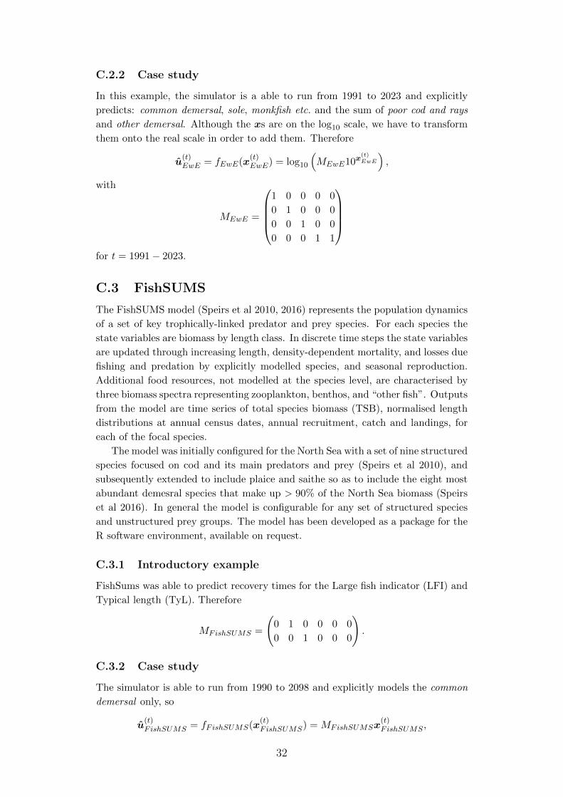
C.3 FishSUMS

The FishSUMS model (Speirs et al 2010, 2016) represents the population dynamics

of a set of key trophically-linked predator and prey species. For each species the

state variables are biomass by length class. In discrete time steps the state variables

are updated through increasing length, density-dependent mortality, and losses due

fishing and predation by explicitly modelled species, and seasonal reproduction.

Additional food resources, not modelled at the species level, are characterised by

three biomass spectra representing zooplankton, benthos, and “other fish”. Outputs

from the model are time series of total species biomass (TSB), normalised length

distributions at annual census dates, annual recruitment, catch and landings, for

each of the focal species.

The model was initially configured for the North Sea with a set of nine structured

species focused on cod and its main predators and prey (Speirs et al 2010), and

subsequently extended to include plaice and saithe so as to include the eight most

abundant demesral species that make up > 90% of the North Sea biomass (Speirs

et al 2016). In general the model is configurable for any set of structured species

and unstructured prey groups. The model has been developed as a package for the

R software environment, available on request.

C.3.1 Introductory example

FishSums was able to predict recovery times for the Large fish indicator (LFI) and

Typical length (TyL). Therefore

MFishSUMS =

(0 1 0 0 0 0

0 0 1 0 0 0

).

C.3.2 Case study

The simulator is able to run from 1990 to 2098 and explicitly models the common

demersal only, so

u(t)FishSUMS = fFishSUMS(x

(t)FishSUMS) = MFishSUMSx

(t)FishSUMS ,

32

with

M3 =(

1 0 0 0 0)

for t = 1990− 2098.

The simulator was “hand tuned” (Speirs et al 2010) to fit observed data in order

to find the optimal parameter set for the model. During this period it became

apparent that the most sensitive parameters were the mortality rate parameters.

For this work we fitted these 4 parameters to landings data from 1990 to 2008. We

assumed that the true landings were normally distributed on the log scale (Tsehaye

et al 2014) and then fitted these parameters using an MCMC sampler (Metropolis

et al 1953; Hastings 1970) to landings between 1990 and 2008.

For the best point in the MCMC algorithm we fitted the fishing mortalities from

2008 until 2013 using a particle filter. We ran 100 parameter sets found using the

Metropolis-within-Gibbs sampler with fishing mortalities fitted to 2008-2013, and

ran it from 1991-2090 with fishing being turned off in 2013.

C.4 Strathclyde End to End

The Strathclyde end-to-end (StrathE2E) marine food web model was designed to

simulate regional scale, macroscopic top-down and bottom-up cascading trophic

effects (Heath et al 2014b). The mathematical formulation is based on a network

of coupled ordinary differential equations representing the entire food web in the

water column and seabed sediments from nutrients and microbes though zooplank-

ton and fish, to birds and mammals, including the effects of advection, mixing and

active vertical migrations. Living components are represented at low taxonomic

resolution, focussing on fluxes of nitrogen between coarse functional groups, and

simulating the general ?shape? of the food web rather than the detail. The scheme

takes off-line output from General Circulation Models (GCM) in the form of volume

and nutrient fluxes through the external boundaries and mixing rates between the

vertical compartments, but is not directly coupled to any GCM. The advantage is

very fast run-times which has enabled the implementation of computational param-

eter optimisation methods to fit the models to observed data, sensitivity analysis

(Morris et al 2014), and computation of likelihoods for model outputs. The focus of

existing uses of Strathe2E has been on UK shelf seas and the cascading implications

of fisheries and fishing practices such as trawling and its impacts on the seabed,

and discarding of unwanted catch (Heath 2012; Heath et al 2014a, 2015).

C.4.1 Introductory example

StrathE2E was able to predict recovery times for b=Birds and mammals (B&M),

Zooplankton to phytoplankton biomass (Z:P) and Zooplankton biomass (ZB). There-

fore

MStrathE2E =

1 0 0 0 0 0

0 0 0 0 1 0

0 0 0 0 0 1

.

33

C.4.2 Case study

The simulator is able to run from 1983 until 2050 and is able to output a sum of

the different groups of species. Although the xs are on the log10 scale, we have to

transform them onto the real scale in order to add them so

u(t)StrathE2E = fStrathE2E(x

(t)StrathE2E) = log10

(MStrathE2E10x

(t)StrathE2E

),

with

MStrathE2E =(

1 1 1 1 1)

for t = 1983− 2050.

In Heath (2012), the simulator was fitted to data using a method of simulated

annealing. For this work we took the parameter values from the simulated annealing

and then used priors from Morris et al (2014) to find the parameters that are most

sensitive. Using derivative-based sensitivity analysis (Sobol’ and Kucherenko 2009,

2010) we calculated upper bounds of the total sensitivity indices for each of the 72

uncertain parameters. We then used MCMC in order to sample from the posterior

distribution of the 12 most sensitive parameters.

We sampled 100 parameter values from the posterior distribution and then,

using the fishing mortalities from the multi species model and the FishSUMs, cal-

culated in Sections C.1 and C.3 and calibrated to the StrathE2E. We ran StrathE2E

to 2013 and then the fishing mortalities were set to 0 before running it until 2050.

C.5 LeMans

The LeMans North Sea model framework (Thorpe et al 2015, 2016, 2017) is an

ensemble of length-structured multispecies models which account for multispecies

interactions and model parameter uncertainty. It is a modified form of the length-

based multispecies model initially developed by Hall et al (2006) to represent the

Georges Bank fish community, and which was subsequently adapted for use in the

North Sea by Rochet et al (2011). The model represents 21 fish species in 32 equal

length classes of around 5cm each, spanning the full size range of species represented

into the model (nearly 200cm for some simulations). Progression of individuals

through length classes is represented by a deterministic von Bertalanffy growth

equation. Individuals mature when they reach a certain size which is defined by a

logistic model, in which 50% of the individuals maturing at the length of maturity

(Lmat see Table S2 in Thorpe et al (2017)). Reproduction is described with a

spawner recruit relationship, which determines the numbers of recruits entering

the smallest size class from the biomass of mature individuals. Species dynamics

are linked via predation mortality (M2) which varies with predator abundance,

and size and species preference. Size preference is described with a preference

function based upon a log-normal distribution and species preference with a diet

matrix indicating who eats whom (Rochet et al 2011; Thorpe et al 2015). In each

length class, individuals are also susceptible to residual natural mortality (M1)

and fishing mortality (F). An ensemble approach is used, based upon a “filtered

ensemble” (FE) of models drawn from a population of 78,125 candidate models

(the “unfiltered ensemble” or UE), with the FE being selected on the basis of

an individual member’s ability to persist stocks when unfished, and to simulate

34

assessed abundances of 10 stocks between 1990 and 2010 to an acceptable degree.

This ensemble approach is described in detail in Thorpe et al (2015), and further

details of the model, including equations are provided in Thorpe et al (2017).

C.5.1 Case study

The simulator was able to predict from 2000 until 2099 and explicitly models:

common demersal, sole, monkfish etc. and poor cod and rays, therefore

u(t)LeMans = fLeMans(x

(t)LeMans) = MLeMansx

(t)LeMans,

with

MLeMans =

1 0 0 0 0

0 1 0 0 0

0 0 1 0 0

0 0 0 1 0

for t = 2000 . . . 2099.

C.6 PDMM

The Population-Dynamical Matching Model (PDMM) constructs complex and population-

dynamically stable ecological model communities at species resolution by mimicking

the natural process of community assembly by successive invasion. Each species is

represented by its dynamic population biomass, and a set of fixed traits that de-

termine food-web structure and physiological parameters. Ontogenetic growth is

modelled implicitly through wide predator-prey size-ratio windows (Rossberg 2012).

The behaviour of consumer individuals is modelled implicitly through Type 2 func-

tional responses extended to incorporate prey switching. Recent variants of the

model were described by Fung et al (2013) and Rossberg (2013).

C.6.1 Introductory example

PDMM was able to predict recovery times for Large fish indicator (LFI), Typical

length (TyL), Fish population biomass trends (FPBT), Zooplankton to phytoplank-

ton biomass (Z:P) and Zooplankton biomass (ZB). Therefore

MPDMM =

0 1 0 0 0 0

0 0 1 0 0 0

0 0 0 1 0 0

0 0 0 0 1 0

0 0 0 0 0 1

.

D Prior distributions for case study

Long-term individual discrepancy

JLB decided that she knew more about the correlations of the outputs between

simulators than she did the absolute differences. Therefore, using the separation

35

method of Barnard et al (2000), the variance of the long-term individual discrep-

ancy, C, was rewritten as

ΣcPcΣc

where Σc is a matrix with the diagonal elements σj > 0 and the off diagonal

elements 0 and Pc is a correlation matrix where the diagonal elements are 1 and

the off diagonal elements are −1 < ρcij < 1. The prior on Pc took the form

p(Pc) = 1Pc�0

n−1∏i=1

n∏j=i+1

fij(ρcij)

where ρcij is the element of Pc on the ith row and jth column and fij is a dis-

tribution determined by elicitation. Using the method of concordance (Gokhale

and Press 1982; Clemen and Reilly 1999) and Shelf R package (Oakley 2015), beta

distributions were fitted to JLB’s prior beliefs about the elements of Pc. These are

shown in Table A1 and samples of the off diagonal elements of Pc are shown in

Figure A1.

Table A1: Beta values found from the elicitation

Com

mon

Dem

Sole

Mon

kfish

etc.

Poo

rco

dan

dra

ys

Oth

erD

em

Common Dem − − − − −Sole 15.865,1.148 − − − −

Monkfish etc. 15.075,1.045 14.168, 2.085 − − −Poor cod and rays 53.996,4.711 19.115,1.628 7.260,1.214 − −

Other Dem 24.853,2.240 14.295,1.706 7.050,1.549 5.712,1.071 −

Using the difference method of Al-Awandhi and Garthwaite (1998), we elicited

JLB’s beliefs of the absolute values of the simulator outputs for each of the groups

species, i.e. the diagonal elements of ΣC . All were given inverse gamma distri-

butions with parameters shown in Table A2. JLB was quite uncertain about the

Table A2: The prior parameters of the inverse-gamma distribution for δ.

a b

Common Dem 100.000 30.801

Sole 100.000 30.943

Monkfish etc. 100.000 23.009

Poor cod and rays 100.000 22.763

Other Dem 100.000 20.110

36

Common demersal

−1.0 0.0 0.5 1.0

02

46

810

Sole

−1.0 0.0 0.5 1.0

02

46

810

Monkfish etc.

−1.0 0.0 0.5 1.0

02

46

810

Poor cod and rays

−1.0 0.0 0.5 1.0

02

46

810

Other Demersal

02

46

810

Figure A1: Samples from the elicited prior distribution of Pc.

37

Common demersal

Log biomass tonnes per km squared

Density

0.25 0.30 0.35 0.40 0.45

02

46

812

Sole

Log biomass tonnes per km squared

Density

0.25 0.30 0.35 0.40 0.45

02

46

812

Monkfish etc.

Log biomass tonnes per km squared

Density

0.20 0.25 0.30

05

10

15

Poor cod and rays

Log biomass tonnes per km squaredD

ensity

0.20 0.25 0.30

05

10

15

Other demersal

Log biomass tonnes per km squared

Density

0.14 0.16 0.18 0.20 0.22 0.24 0.26 0.28

05

10

15

20

Figure A2: Samples from the prior of diagonal elements of ΣC .

values of µ(2010) so for numerical stability we capped a to be 100. Samples from

the variance, the diagonal elements of ΣC , are shown in Figure A2.

Shared discrepancy

JLB did not believe that the model average overestimated the truth any more than

it underestimated it so δ ∼ N(0, I), where I is the identity matrix. She was not sure

what the standard deviation in equation 4 was so she put quite an uninformative

prior,

(diag(∆ζ))0.5 ∼ Exponential(5),

and the correlation terms were uniformly distributed between -1 and 1. She thought

that the standard deviation in equation 5 was a bit smaller but was still quite unsure

about its value so

(diag(∆µ))0.5 ∼ Exponential(1),

with correlation terms were uniformly distributed between -1 and 1. kµ, the rate

at which the covariance decreases was uniformly distributed on [0, 6].

38

ki

Density

0 1 2 3 4 5 6

0.0

0.1

0.2

0.3

Rij

Density

-0.5 0.0 0.5 1.0

0.0

0.5

1.0

1.5

2.0

ρijk

Density

-1.0 -0.5 0.0 0.5 1.0

0.0

0.1

0.2

0.3

0.4

0.5

0.6

0.7

πij

Density

0.0 0.5 1.0 1.5 2.0 2.5 3.0

0.0

0.1

0.2

0.3

0.4

0.5

Figure A3: Samples from the elicited hyper-priors.

Hyper-parameters

JLB elicited her prior beliefs for the hyper-parameters ki, Rij , πij and ρijk for

j = 1, . . . , 5, k = 1, . . . , 5 and j 6= k. She believed that for all j and k the

distributions were exchangeable a priori, thus the prior predictive distributions

were the same for all j and k. Samples from the prior predictive distributions are

shown in Figure A3. The hyper-priors were tuned so that they would lead to prior

predictive distribution of JLB shown in Figure A3.

JLB expected that models would reach equilibrium slower than in one step.

However she was not quite sure how fast that would happen so she set quite an

uninformative priors on ki. By thinking about the rate by which the variance

declines, exp ki, the priors were elicited to be

ak ∼ Gamma(10, 10)

and

bk ∼ Gamma(10, 5).

A priori, JLB did not know what values the diagonals of Ri but suggested that

they would be positive so

aR ∼ Gamma(10, 5)

39

and

bR ∼ Gamma(10, 10).

Similarly, JLB expected πj to be small. Therefore

απ,j ∼ Gamma(15, 10)

and

απ,j ∼ Gamma(10, 2).

JLB was unsure about values of ρjk and therefore

aρjk, bρjk ∼ Gamma(10, 10).

E Correlation of the future groups

The correlations of the relative truth of the future groups in 2025 and 2050 are

shown in Tables A3 and A4 respectively.

Table A3: The correlation of the relative truth for the future groups in 2025.

Com

mon

Dem

Sole

Mon

kfish

etc.

Poo

rco

dan

dra

ys

Oth

erD

emCommon Dem 1 0.156 0.281 0.263 0.023

Sole 0.156 1 0.285 0.134 0.001

Monkfish etc. 0.281 0.285 1 0.290 -0.017

Poor cod and rays 0.263 0.134 0.290 1 -0.025

Other Dem 0.023 0.001 -0.017 -0.025 1

40

Table A4: The correlation of the relative truth for the future groups in 2050.

Com

mon

Dem

Sole

Mon

kfish

etc.

Poo

rco

dan

dra

ys

Oth

erD

em

Common Dem 1 0.138 0.306 0.172 0.011

Sole 0.138 1 0.273 0.154 0.011

Monkfish etc. 0.306 0.273 1 0.253 0.023

Poor cod and rays 0.172 0.154 0.253 1 -0.010

Other Dem 0.011 0.011 0.023 -0.010 1

41