Embed Size (px)
Citation preview

MULTI-MODAL VIDEO SUMMARIZATION
USING HIDDEN MARKOV MODELS
FOR CONTENT-BASED MULTIMEDIA INDEXING
A THESIS SUBMITTED TO
THE GRADUATE SCHOOL OF NATURAL AND APPLIED SCIENCES
OF
THE MIDDLE EAST TECHNICAL UNIVERSITY
BY
YAĞIZ YAŞAROĞLU
IN PARTIAL FULFILMENT OF THE REQUIREMENTS FOR THE DEGREE OF
MASTER OF SCIENCE
IN
THE DEPARTMENT OF ELECTRICAL AND ELECTRONICS ENGINEERING
SEPTEMBER 2003

Approval of the Graduate School of Natural and Applied Sciences
______________________
Prof. Dr. Canan Özgen
Director
I certify that this thesis satisfies all the requirements as a thesis for the degree of
Master of Science.
______________________
Prof. Dr. Mübeccel Demirekler
Head Of Department
This is to certify that we have read this thesis and that in our opinion it is fully
adequate, in scope and quality, as a thesis for the degree of Master of Science.
______________________
Assoc. Prof. Dr. A. Aydın Alatan
Supervisor
Examining Committee Members
Assoc. Prof. Dr. Tolga Çiloğlu ______________________
Assoc. Prof. Dr. Gözde Bozdağı ______________________
Assoc. Prof. Dr. Buyurman Baykal ______________________
Assoc. Prof. Dr. A. Aydın Alatan ______________________
Prof. Dr. Enis Çetin ______________________
iii
ABSTRACT
MULTI-MODAL VIDEO SUMMARIZATION
USING HIDDEN MARKOV MODELS
FOR CONTENT-BASED MULTIMEDIA INDEXING
Yaşaroğlu, Yağız
MSc., Department of Electrical and Electronics Engineering
Supervisor: Associate Professor A. Aydın Alatan
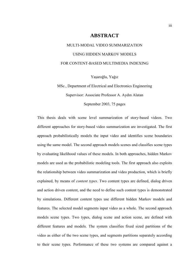
September 2003, 75 pages
This thesis deals with scene level summarization of story-based videos. Two
different approaches for story-based video summarization are investigated. The first
approach probabilistically models the input video and identifies scene boundaries
using the same model. The second approach models scenes and classifies scene types
by evaluating likelihood values of these models. In both approaches, hidden Markov
models are used as the probabilistic modeling tools. The first approach also exploits
the relationship between video summarization and video production, which is briefly
explained, by means of content types. Two content types are defined, dialog driven
and action driven content, and the need to define such content types is demonstrated
by simulations. Different content types use different hidden Markov models and
features. The selected model segments input video as a whole. The second approach
models scene types. Two types, dialog scene and action scene, are defined with
different features and models. The system classifies fixed sized partitions of the
video as either of the two scene types, and segments partitions separately according
to their scene types. Performance of these two systems are compared against a

iv
deterministic video summarization method employing clustering based on visual
properties and video structure related rules. Hidden Markov model based video
summarization using content types enjoys the highest performance.
Keywords: Video summarization, hidden Markov models, content-based indexing.

v
ÖZ
İÇERİK TABANLI ÇOKLUORTAM ENDEKSLEMESİ İÇİN
SES VE GÖRÜNTÜ BİLGİSİ YARDIMIYLA
SAKLI MARKOV MODELİ KULLANARAK VİDEO ÖZETLEME
Yaşaroğlu, Yağız
Yüksek Lisans, Elektrik ve Elektronik Mühendisliği Bölümü
Tez Yöneticisi : Doçent Dr. A. Aydın Alatan
Eylül 2003, 75 sayfa
Bu tez çalışması öyküye dayanan videoların sahne seviyesinde özetlenmesi üzerine
bir çalışmadır. Probleme iki ayrı bakış açısından yaklaşılmıştır. Birinci yaklaşım
videoların bütün halinde modellenmesini öngörmektedir. Elde edilen model
yardımıyla sahne sınırları belirlenmektedir. İkinci yaklaşım farklı türdeki sahneler
için modeller oluşturulmasına ve videonun analizi sırasında sahne türlerinin
belirlenmesine dayanmaktadır. Her iki yöntemde de kullanılan modeller saklı
Markov modelleridir. Birinci yöntemde tez kapsamında kısaca değinilen video
özetleme ile video prodüksiyonu arasındaki ilişkiden yararlanmak için içerik türleri
tanımlanmıştır. Sistemde iki içerik türü gerçeklenmiş (hareket ağırlıklı içerik ve
diyalog ağırlıklı içerik) ve yapılan deneylerde gereklilikleri doğrulanmıştır. Farklı
içerik türleri farklı saklı Markov modelleri ve öznitelikler kullanmaktadır. İçerik
türüne göre seçilen model videoyu bir bütün olarak işleyip bölütlemektedir. İkinci
yöntemde ise sahne türleri modellenmektedir. Farklı modeller ve öznitelikler
kullanan iki sahne türü belirlenmiştir: hareketli sahneler ve diyalog sahneleri. Girdi
videonun sabit uzunluktaki parçaları iki sahne türünden birisine sınıflanır, ve her

vi
parça ayrı ayrı sahne türüne göre bölütlenir. İki yöntemin performansı görsel
öselliklere ve video yapısıyla ilgili kurallara dayanan bir topaklama metoduyla
karşılaştırılmıştır. Saklı Markov modelleri kullanarak içerik türüne bağlı video
özetleme en iyi performansa sahiptir.
Anahtar kelimeler: Video özetleme, saklı Markov modelleri, içerik tabanlı
endeksleme.

vii
ACKNOWLEDGMENTS
I would like to acknowledge the skillful supervision and supreme vision of
Assoc. Prof. Dr. Aydın Alatan, both of which were crucial to development of this
thesis; and the valuable comments of examining committee members Assoc. Prof.
Dr. Tolga Çiloğlu, Assoc. Prof. Dr. Gözde Bozdağı, Assoc. Prof. Dr. Buyurman
Baykal and Prof. Dr. Enis Çetin.
I would like to thank my family for their unwavering support.
I would like to raise my glass to my “Brothers in Arms,” and to Cağlar, Ekin
and Onur, and to my friends at EnkarE for our long lasting friendship and the
bottomless well of inspiration.

viii
TABLE OF CONTENTS
ABSTRACT ................................................................................................................iii
ÖZ ............................................................................................................................ v
ACKNOWLEDGMENTS..........................................................................................vii
TABLE OF CONTENTS ..........................................................................................viii CHAPTER
1 INTRODUCTION ...........................................................................................10
1.1 Scope of the Thesis...................................................................................11
1.2 Outline of the Thesis ................................................................................12
2 VIDEO SUMMARIZATION ..........................................................................14
2.1 Problem Domain.......................................................................................14
2.2 Structure of a Video .................................................................................16
2.3 Overview of the Problem ......................................................................... 20
2.4 Related Work............................................................................................ 21
3 PROBABILISTIC REASONING.................................................................... 26
3.1 Discrete Markov Processes and Extension to HMMs .............................. 28 3.1.1 Discrete Markov Processes........................................................... 28 3.1.2 Hidden Markov Models................................................................ 30
3.2 Basic Problems for Hidden Markov Models ............................................ 32
3.3 Solution to Basic Problems of HMMs ..................................................... 33 3.3.1 Problem 1 ..................................................................................... 33 3.3.2 Problem 2 ..................................................................................... 34 3.3.3 Problem 3 ..................................................................................... 35

ix
4 PROPOSED VIDEO SUMMARIZATION SYSTEM.................................... 38
4.1 Overview of the System ........................................................................... 38
4.2 Content Types........................................................................................... 39 4.2.1 Dialog-Driven Content ................................................................. 40 4.2.2 Action-Driven Content ................................................................. 41
4.3 Preprocessing............................................................................................ 41
4.4 Feature Extraction Stage .......................................................................... 42 4.4.1 Face Detection .............................................................................. 43 4.4.2 Audio Analysis ............................................................................. 45 4.4.3 Location Change Analysis............................................................ 51 4.4.4 Motion Activity Analysis ............................................................. 53
4.5 Decision Making Stage ............................................................................ 54
4.6 Models ...................................................................................................... 55
4.7 Training .................................................................................................... 57
5 SIMULATIONS............................................................................................... 60
5.1 Feature Extractor Performance Simulations............................................. 61
5.2 Content Type Simulations ........................................................................ 62
5.3 Scene Modeling Simulations.................................................................... 66
5.4 Comparison With Deterministic Approach .............................................. 68
5.5 Evaluation of the Results.......................................................................... 69
6 CONCLUSIONS.............................................................................................. 70
REFERENCES........................................................................................................... 73

10
CHAPTER 1
INTRODUCTION
Rate of digital content creation and duplication has increased. The Internet Movie
Database reports that in their database there are 10128 movie titles produced in 2002,
93422 in the last decade [1], and that is only the movie industry. Amount of daily
content created by TV channels over the world cannot be measured: On-site news
shooting, in-studio programs, sports event broadcasts, in-house produced films,
serials, documentaries, and other production jobs, broadcasted everyday to homes of
billions. However, content creation is not in the monopoly of studios or production
firms. Dyne:bolic, a single bootable CD Linux distribution, collects a wide array of
open source digital content creation tools, from recording utilities to video/audio
editing tools and web-broadcasting applications [2]. It enables any sufficient
computer to become a studio, managed by ordinary users. All the while the Internet,
with its decentralized, end-point centered architecture, enables millions of netizens to
share digital content with unprecedented ease, despite all attempts to strangle it.
Advanced mobile and multimedia technologies, such as web-enabled cellular phones,
multimedia messaging and media streaming allow people to interact with multimedia
data everywhere. Digital content is ubiquitous.

11
This increased generation and distribution rate of audiovisual content created
a new problem: management of the content. Unlike tools to create and distribute,
tools to manage multimedia content are not mature enough. Neither there is a
feasible way to automatically analyze and classify content, nor browsing the content
is easy. As a matter of fact, current solutions to large scale multimedia content
database management are usually meta-data driven. For example, Turkish Radio and
Television (TRT), having the largest video archive in Turkey, relies on
unstandardized, ad hoc information about the video, entered by the producer of the
video, and possibly remembered only by him. As another approach, an attempt to
label all multimedia content in such a large-scale database manually, uniformly
according to a standard is both infeasible and error-prone. The most widespread
solution other than meta-data generation is traditional linear browsing through
multimedia content. Unfortunately, this solution is too tedious.
Automatic video summarization emerges as a solution to the problem of
managing video content. Automatic video summarization can be defined as
identifying relevant parts of a video and presenting it in an easily browsable form,
with minimal user intervention [3].
1.1 Scope of the Thesis
This thesis deals with scene level summarization of story based videos using hidden
Markov models. Two different approaches to summarization are implemented: Video
modeling and scene modeling. In both cases four features are extracted from the
video stream for each shot in the video: Face existence, audio class, location change
existence and motion activity level. In both cases the feature sequence vector is used
12
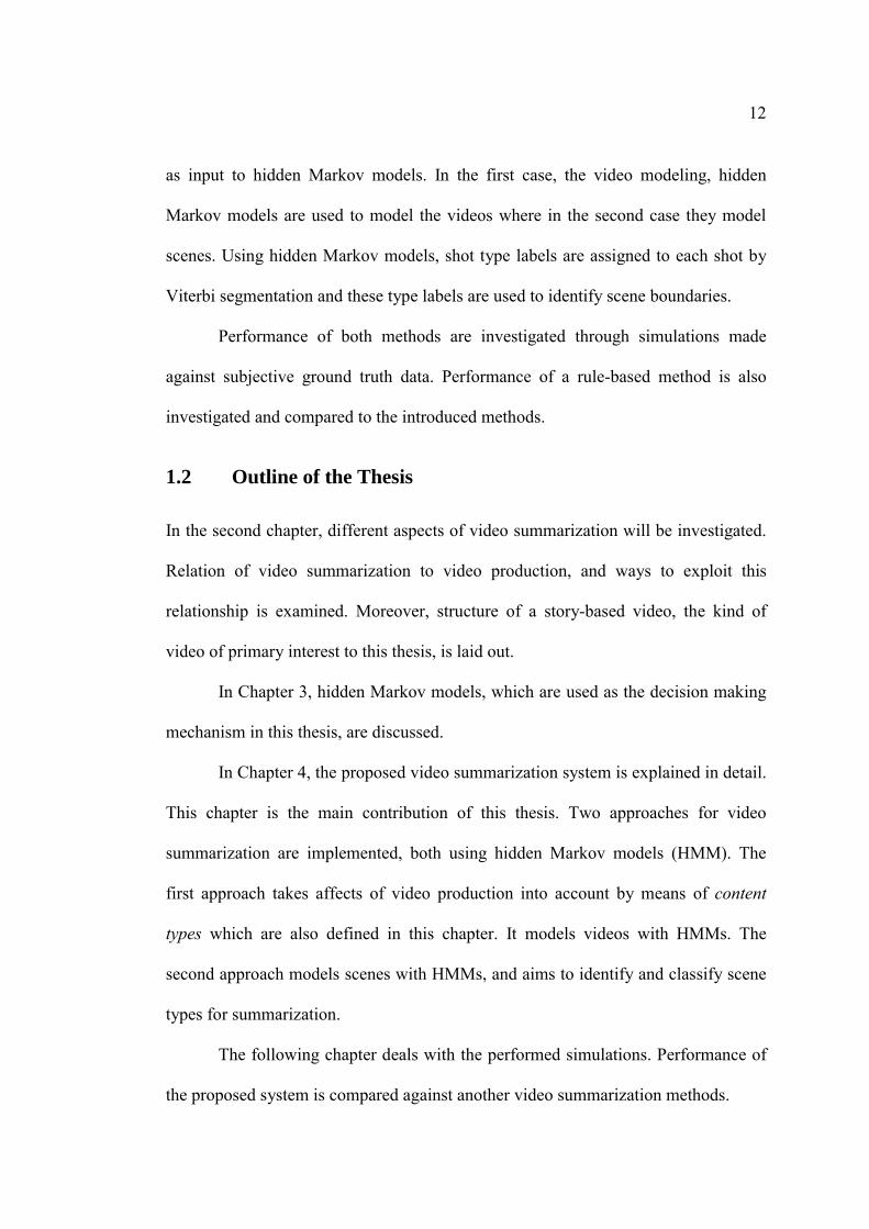
as input to hidden Markov models. In the first case, the video modeling, hidden
Markov models are used to model the videos where in the second case they model
scenes. Using hidden Markov models, shot type labels are assigned to each shot by
Viterbi segmentation and these type labels are used to identify scene boundaries.
Performance of both methods are investigated through simulations made
against subjective ground truth data. Performance of a rule-based method is also
investigated and compared to the introduced methods.
1.2 Outline of the Thesis
In the second chapter, different aspects of video summarization will be investigated.
Relation of video summarization to video production, and ways to exploit this
relationship is examined. Moreover, structure of a story-based video, the kind of
video of primary interest to this thesis, is laid out.
In Chapter 3, hidden Markov models, which are used as the decision making
mechanism in this thesis, are discussed.
In Chapter 4, the proposed video summarization system is explained in detail.
This chapter is the main contribution of this thesis. Two approaches for video
summarization are implemented, both using hidden Markov models (HMM). The
first approach takes affects of video production into account by means of content
types which are also defined in this chapter. It models videos with HMMs. The
second approach models scenes with HMMs, and aims to identify and classify scene
types for summarization.
The following chapter deals with the performed simulations. Performance of
the proposed system is compared against another video summarization methods.

13
In the final chapter conclusive remarks and thoughts about future work are
given.

14
CHAPTER 2
VIDEO SUMMARIZATION
2.1 Problem Domain
There is diverse distribution of video with respect to relevant semantic content.
Video with lowest amount of meaningful content is surveillance video, since the
relevant content is only the existence and identity of an intruder. More meaningful
content can be found in sports event videos, documentaries, news broadcasts,
advertisements and home videos with varying amount. However, the highest amount
of semantics is in story-based videos. This kind of videos has a content based on a
story line; they tell a meaningful story.
In addition to variety in amount of relevant content, there is also variety in
techniques of presentation among videos as well. Content is transformed into a video
through a process that is to be called production. In the context of this thesis,
production's input is the content, and its output is the video. Anything that affects the
final output is in the scope of production. It includes the camera in a surveillance
video, or the writing of the script, acting, shooting, and editing in a movie.
Importance of production lies in the fact that differently produced videos are
perceived differently. Two versions of the same movie can be remarkably different

15
due to differences in casting, directing, and editing. Even regular and “director's cut”
versions of the same movie, shot with the same cast by the same director, are distinct
movies. Impact of production on the final output is powerful.
On the other hand, production has guidelines and conventions that limits and
advises a producer. According to these guidelines, some video types are produced in
a fixed way. For example, the presentation of a news program is similar to other
news programs. An anchorman reads out a news item followed by the video clip
related to the item. Sports event videos are also examples to videos of this sort. A
soccer match is always recorded in the same way, with reverse angle shots, instant
replays, and so on.
Contrary to these, some video types, such as movies are produced more
freely. However, they still rely on conventions and guidelines that are recognized by
the audience. Producers use these guidelines to get across their message to the
audiance.
The semantic content diversity and production variety mentioned above
necessitates different summarization approaches to be developed. For example,
summarizing surveillance video may only consist of identifying parts of the video
that contain the subject; robbery or intruder. On the other hand, summarizing soccer
video might be possible by detecting goals and near-miss situations, and other events
in the video that may be considered important by a viewer, such as bookings. In
order to summarize story-based video, an automatic system might be built that
catalogs parts of the video that tell an unbroken part of the story. A frame or a short
clip can then be displayed in place of each story part, summarizing the video.

16
In order to identify important events in a soccer video, an automatic system
might exploit the production methods unique to the domain, and detect slow motion
replays in the video. Or the properties of the content can be exploited: The audio
signal can be analyzed to identify the portions that have loud spectator noise.
In order to detect an intruder, the fact that a surveillance camera is targeted at
a fixed location for a long period of time can be used. The background of the scene
can be learned and the presence of an intruder can be deduced. In this situation, the
behavior of the camera is a production property, while the background being fixed is
a property of the content.
Production patterns and properties of the content being produced can be used
to develop automatic summarization systems. Videos that share production patterns
can be summarized using similar techniques; while it must be kept in mind that even
videos that are produced in the same way have differences that will make
summarization more challenging.
This thesis proposes two video summarization methods. One of the methods
exploits production and content similarities between videos and the other relies on
different properties of the scenes. Both methods’ performances are compared against
a clustering based summarization method.
2.2 Structure of a Video
Throughout this thesis, the term 'video' is used to refer to the combination of an
image sequence and its associated audio stream.
Continuous recording of a single camera in a video is called a 'shot' [4]. Shots
are the semantic building blocks in story-based videos. While editing raw shooting,

17
editors divide the raw video into shots and combine these shots to build a story flow.
Shots are analogous to letters in a language; in other words, they don't have meaning
on their own, but they gain meaning as a sequence [5]. Single-shot scenes are
exceptions, just like single letter words.
A collection of shots that are temporally adjacent and semantically related is
called a 'scene.' Scenes are sometimes called story units, in that they tell a part of the
story that takes place in a fixed location, happens within a fixed time frame, involves
a fixed list of people, or has a combination of these. Another characteristic of scenes
is that a temporary resolution is reached within them [6].
For example, in the movie “Blade Runner,” there is a scene in which the main
protagonist Deckard eats at a Chinese street bar. The first time the viewer meets
Deckard is when the camera approaches him through the crowd in the street, and
finds him reading a newspaper. In the next shot, we see the bar, and the next few
shots are used to set up the place and time. At the seventh shot, Deckard gets up and
crosses the street to sit at the bar. Four more shots are spent while he orders his meal.
And finally after getting his meal, at the fourteenth shot, a cop comes and in seven
more shots we learn that a certain Captain Bryant is looking for Deckard. Scene ends
with Deckard smiling to himself knowingly.
The entire scene, a rather short one, lasts for twenty-one shots. Scene's time is
fixed as well as the location, the street, but people involved in the scene change as
shots progress. Deckard's smile provides the resolution by telling the viewer that he
is not nervous, and releases the tension created by appearance of the cop.
Note that none of the shots by itself is able to move the story forward. Each
shot provides background information, they help the user to form an idea of the
18
place, the people, the things in the video, but shots by themselves do not have
enough meaning to tell a story. However, when a shot is viewed within the context
created by related shots, it becomes meaningful, and it can move the story forward
[5].
In the above example, the shot that shows a cop appearing beside Deckard
does not carry enough meaning by itself. The viewer does not know where Deckard
is, does not know if the cop was around before, does not know if they have met
before, does not know either one's purpose, and so on. Some of these mysteries are
resolved, and the shot gains meaning, upon viewing the shots that come before and
after it. It is learned they have not met before, cop has come to take Deckard to the
police station and Deckard is not worried about it. All of this information along with
details about the story (Deckard is eating Chinese food, the cop cannot speak
English, it is raining, etc.) are told to the viewer only by the help of related shots.
Shots that are adjacent in time and semantically related from scenes, and the story is
told by scenes.
This relationship between shots and scenes has its roots in 'Film Grammar'.
Film grammar is a collection of accepted rules and techniques which directors use to
transfer the story form text to video [7]. Audiences worldwide are used to these
techniques, and by employing them, directors are able to make viewers perceive the
movie as a continuous experience, despite the appearance of several shot cuts each
minute [8].
There are three types of scenes in story-based videos: Action scenes, dialogue
scenes and dialogue scenes with action [6]. The director has infinite freedom over
how to shoot a scene, but film grammar suggests a scheme.
19
A scene starts with an establishing shot. An establishing shot is usually a
wide-angle view of the location, introducing the protagonists and their position in the
scene. Different views of the conversing people, or the people participating in the
action are shown as the scene progresses. The views are usually shot from varying
distances, and the director may choose to show people in groups of different
numbers, in order to break the monotony of the scene. In a dialogue scene, the
camera gradually approaches people as a conversational climax is reached, and it
backs up as a release. Re-establishing shots may be shown in the middle of the
scenes to remind the location, the protagonists; or just as a break of monotony.
Close-up shots of relevant objects in the scene, or views of relevant objects or places
out of the scene can be shown. A scene usually ends with a re-establishing shot that
acts as a conclusion to the scene [6].
Another important component of a video signal is the information stored in
its audio part. Humans can understand what is happening in a movie only by
listening to the audio track. The audio track contains speech, sound effects, music
and environmental sound. Speech may belong to a conversation, or to a narrator.
Sound effects accompany actions like walking or shooting. Music can be used to set
a mood (creepy music), or signal an event or location (birthday, wild west).
Environmental sound is used to support the reality of the story.
Speech is dominant in dialogue scenes. Usually all sounds are suppressed in a
dialogue scene to keep the attention on the speech. Sound effects and mood setting
music are most prominent in action scenes. Environmental sound and music used as
introduction are strongest in establishing shots.
20
These properties of scenes, various shot types and relation between scenes
and shots can be used to develop a method of video summarization.
On average, a film is made up of around 50 scenes, each having about 40
shots [5]. Adding this to the fact that shots in a scene are semantically related to each
other, it becomes apparent that scenes are more suitable to summarization of story-
based videos. Actually, when humans summarize a movie, they tend to tell the story
scene by scene (e.g. Bryant greeted Deckard, and told him about four Replicants he
needed to get retired) rather than shot by shot (e.g. Deckard came into the room and
looked at Bryant. Bryant said “Hi ya, Deck.” Deckard replied “Bryant...”), as well.
Summaries constructed using shots would be long and redundant, whereas scene-
based summaries would be concise.
2.3 Overview of the Problem
The problem of automatic video summarization requires machines to identify the
'relevant' parts in a given video and present them in an easily accessible way. The
difficulty of this problem lies in the task of automatically extracting meaningful
information from digital data streams.
What can be automatically extracted from multimedia content is semantically
low-level, in that the extracted clues have a relatively low amount of meaning by
themselves. Examples are pitch, tempo or energy of sound signals, color, texture or
shape information of visual signals, temporal relationships between signals, and
similar information that can be obtained analytically or algorithmically. On the other
hand, what is required from automatic systems is higher-level semantics, such as
“Beethoven's 9th Symphony,” “red sports car,” “dialogue scene at 12:20.” An

21
example that stresses this point is work by Smith and Chang, which states that 95%
of the queries submitted to their search system VisualSEEK were semantic queries
[3].
In the case of story-based video summarization, the first step to climb in the
semantic ladder is detecting and isolating shots. As shots are the semantic building
blocks of a story-based video, taking representative frames from each shot is a way
to build a summary of the video. However, due to reasons explained previously, shot
level summaries are not desirable, and in order to reach more useful and concise
summaries, they need to be refined.
This refinement comes in the form of scene level video summarization.
Although there is a large body of literature on shot boundary detection [9], efforts on
automatic scene level video summarization have still not reached a conclusive
solution.
2.4 Related Work
Various methods for automatic shot boundary detection have been put forward [9].
Since the visual properties on two sides of a shot boundary are expected to be
different, it is usually visual properties that are exploited. These properties can be
pixel differences or histogram differences of consecutive frames, number of changed
edges in two consecutive frames, standard deviation of pixel intensities, contrast and
so on [9]. Note that some of these features are more suitable to detect ‘cut’ type of
scene boundaries, whereas others are specialized on detecting ‘fades’ or ‘dissolves.’
Applying thresholds to these features can be sufficient to get scene boundaries [9].

22
On the other hand, multiple features can be combined using classifiers so that a better
detection is achieved [10].
If current research trends in scene level video summarization are investigated,
it is seen that there are three main approaches to the problem:
• Object identification based approaches,
• scene type recognition based approaches, and
• video structure analyzing approaches.
Object identification methods generally aim to index video by identifying
objects, producing object-based search opportunities. For example in [11], each shot
is analyzed and its object-related properties are extracted. Depending on
compositional conventions prevalent in video production and utilizing a Bayesian
belief network, the authors determine the “focus of attention”, the object that
receives the most attention from the viewer. Interactions between objects are also
determined [11]. These allow detailed object-based descriptions of shots to be made.
Another object identification based method is explained in [12]. The concept of
probabilistic multimedia objects, “multijects,” which are summarizations of time
sequences of features that are extracted from multiple media, are introduced [12].
Multijects can be objects (e.g. car, helicopter, man), sites (e.g. forest, beach,
outdoor), or events (e.g. explosion, ball-game). They are probabilistically modeled,
with hidden Markov models and Gaussian mixture models, depending on them
having temporal support or not respectively. They are allowed to interact, affecting
likelihood values of each other. For example, presence of the multiject ‘snow’ makes
the presence of the site ‘outdoor’ more likely, and the site ‘underwater’ less likely.
This interaction is modeled by a factor graph [12]. In the end, meta data in the form

23
of keywords are attached to the video stream, giving the multijects’ likelihood, and
spatio-temporal support.
The second approach is to classify scene types in a video. For example, the
method explained in [13] involves building finite state machines for action or dialog
scenes involving two people. Spatial arrangement of actors and camera positioning
are the used features, and state machines are built according to observations made on
dialog scenes and action clips, from the production point of view. Due to the fact that
action scenes and dialog scenes are identical according to used features, authors use
another criterion to classify scenes: average length of shots within a scene. Input
videos are parsed with the state machines, and each scene’s average shot length is
calculated, effectively identifying and classifying scenes.
Controlled Markov chains are used to model temporal evolution of goals and
non-goal situations in soccer videos in [14], thereby identifying goals in the video.
All events are assumed to be two shots long. For each goal and non-goal situation
(free kick, corner kick, etc), the camera motion properties (fast pan, fast zoom and
lack of motion) of two consecutive shots are modeled in the controlled Markov
chains. Likelihood value of each shot pair in the input video being generated by each
Markov chain is calculated, and the chain that gives the highest likelihood
determines the type of the situation. In order to further refine the classification, the
pairs that have been classified as goals are ordered according to the amount of audio
loudness increase between the shots. This ordering carries goal situations higher up
in the ordered list [14].
Similarly, in [15], authors develop hidden Markov models that represent
different scene types particular to baseball matches. The method is based on the idea

24
that due to the production style of baseball videos most baseball highlights are
composed of certain types of shots [15]. An edge descriptor that detects highly
textured regions, color descriptors that detect the amount of grass and sand, camera
motion descriptor, field shape descriptor and player height descriptor are used as
features. Four models are developed for different ‘interesting’ situations in a baseball
match. After features for each scene shot is extracted, the likelihood of each model
for each scene in the baseball video are calculated using the Viterbi algorithm, and
for each scene, the most likely model dictates the scene type.
An approach that models the entire structure of the video is in [16]. It uses
hidden Markov models for capturing the structure of documentary videos, in their
entirety. The features that are extracted and used as hidden Markov model
observations for each shot are the shot type (static image, video clip or commentator)
and camera motion (static, zoom and pan). Through training hidden Markov models
with various topologies using the observations extracted, the authors analyze
structures of various documentary videos. The conclusion reached is that there are
structural differences not only between video genres but also within genres [16].
Another approach described in [17] uses a hidden Markov model that imitates
the structure of dialogue scenes in story-based videos. Audio-visual features are
used; existence of faces and audio class (speech, music, silence) are extracted for
each shot. The observation sequence, which is nothing but the string of features for
all shots, is segmented by the model using Viterbi algorithm, and captures dialog
scene boundaries [17].
In [18] an unsupervised clustering method is used to generate table of content
of a given video. The method uses histogram-based visual similarity and activity

25
similarity measures. Histogram distances of the first and the last frames of each shot
is used as visual similarity measures, whereas the average histogram distance
between consecutive frames of a shot is utilized to be the activity value of the shot
[18]. Using these measures, color similarities and activity similarities between the
shots are calculated, taking into account their temporal differences. These shot
similarities are used to cluster shots into groups using an “intelligent unsupervised
clustering technique,” which takes into account both the similarity measures, and the
structure of the video. Basically, similar groups of shots that are interleaved in time
are merged together [18]. As a result, a table of contents of scenes is generated. This
method is compared against the proposed methods in this thesis. Results of
comparisons are given in Section 5.4.

26
CHAPTER 3
PROBABILISTIC REASONING
Methods used in automatic reasoning can be classified into two categories: rule-
based methods and stochastic methods [19]. Rule-based methods create a database of
rules, which may have truth values attached, that define the environment and the
ways with which these rules interact with each other. On the other hand, stochastic
approaches attach uncertainties to “states of affairs” [19].
The locality and uniformity of interactions of rules are what makes rule-based
systems attractive. If the interactions are simple enough, it is very easy to go through
a list of rules and reach a conclusion. For example, a rule based system might define
rules such as “birds fly,” “pigeon is a bird,” and so on. This way, starting from the
information that something is pigeon, it is very easy to reason that it flies. One
shortcoming of rule-based systems is the need to define exceptions to rules, such as
“birds that are not ostriches, penguins, kiwis or dodos fly” (Actually it should
approximately be “birds that are not ostriches, penguins, kiwis, dodos, chickens,
turkeys, too young, injured or dead fly”). Still, if the rule base is well defined, and
the environment is not changing, the reasoning process will be hassle-free.

27
However, it is also the rules and interactions of them that are the drawbacks
of rule-based systems. First of all, using rules that interact uniformly strips one the
ability of two-way reasoning - if A implies B, presence of B makes A more credible,
and if A and C implies B, if B is present, finding out that A is true makes C less
credible. If, for example, two rules are written such as “fire implies smoke,” and
“smoke makes fire more credible,” these two rules would create a cycle and provide
feedback to each other without any evidence but smoke. Implementing bidirectional
inference required for these kinds of reasoning would mean sacrificing
computational ease, as it would require brute force analysis of all rules and
exceptions. Instead, most systems cut off cycles, permitting one-way inference [19].
Another advantage that is also a drawback concerning rule-based systems is
locality. Rules interact locally; “if A is true then B (with certainty c)” means no
further analysis is needed to assert B if A is known. Although providing
computational ease, this property ignores possibility of correlated evidences. Assume
a rule structure such as:
• If A is true then C is more credible,
• If A is true then B is more credible,
• If C is true then D is more credible,
• If B is true then D is more credible,
• If Z is true then C is more credible.
In such a case, when A is found to be true, it will affect D's credibility
through both B and C, although the evidences of B and C are the same. Again brute
force analysis of all rules is an impractical solution for this problem.

28
On the other hand, a stochastic system makes a declaration about the state of
affairs, saying “most birds fly” with a statement such as pBAP =)( . This statement
is much cleaner than those made by the rule based system, as no exceptions are
required. Also, bi-directional inference and correlated evidence are built-in features
of Bayesian methods [19]. However, in this form, the stochastic statement is nothing
more than an observation about the world. It is not suitable for making reasoning.
Mechanisms that combine stochastic declarations and make decisions should be
used. One such mechanism is the hidden Markov model.
3.1 Discrete Markov Processes and Extension to HMMs
3.1.1 Discrete Markov Processes
A continuous-time, continuous-state Markov process is characterized by the
following equation:
nnnnnnnn tttxxtxPtttxxtxP <≤=≤≤ −−− 111 ],)()([]),()([ .
The essence of this equation is that, in the Markov process )(tx , the past has
no influence on the future, if the present is specified [20]. If nttt <<< �21 , it
follows that
])()([])(,),()([ 111 −− ≤=≤ nnnnnn txxtxPtxtxxtxP � .
Discrete-state Markov processes, where the system can occupy a finite or
countably infinite number of states, is called a Markov chain. Markov chains are
useful in modeling systems that can be described as being in one of a set of states at
any time, undergoing state changes according to a set of probabilities associated to

29
the current state [21]. If the time instants at which state changes happen are regularly
spaced, the Markov equation can be written as
][],,[ 121 injnkninjn SxSxPSxSxSxP ====== −−− l ,
where state changes happen at nTtn = , and the process nx can occupy the
states NSSS ,,, 21 l . Furthermore, the state transition probabilities, the right-hand
side of the equation, are assumed to be time-invariant. They are denoted as:
][ 1 injnij SxSxPa === − .
ija is the time-invariant state transition probability from state j to state i, and
it obeys the standard stochastic rules:
0≥ija ,
∑=
=N
jija
1
1 .
In order to clarify the definitions, consider the following example:
A simple discrete Markov chain is used to model the weather. It is assumed
that weather can occupy one of the three states SUNNY (state 1), RAINY (state 2)
and SNOWY (state 3) at any time )3( =N . See the Markov chain diagram in Figure
1.
Observations are assumed to be made once a day. Note the transition
probabilities ija labeling transition arrows on the figure. Actual values for transition
probabilities can be determined by observing the weather for a given period of time
and counting the number of transitions from state i to state j and dividing that number
by the total number of transitions from state i.

30
0SUNNY
1RAINY
a11
a10
a01a00
2SNOWY
a12a21a02a20
a22
Figure 1. Example discrete Markov chain.
What this simple model gives us is the ability to make predictions about the
weather by only knowing the current state. For example, if the current state is
SUNNY, then the probability that it will rain tomorrow is 21a .
3.1.2 Hidden Markov Models
Before examining hidden Markov Models (HMM), consider a simple model for
climate. Assume seasons are to be modeled, but the date is unknown. The only
available information is whether the weather is SUNNY, RAINY, or SNOWY. This
kind of a process, where the states are not observable, but a separate set of features
are available for observation, is more suitable to be modeled by a hidden Markov
model. States and state transition probabilities from discrete Markov processes are
preserved in hidden Markov models. Observations are added as probabilistic
functions of the state, and unlike discrete Markov processes, states are not
observable. Idea is that the stochastic process being modeled can only be observed
through another stochastic process.
In an HMM consisting of N states, state transition probabilities are shown by
an N by N state matrix A, whose elements ija are the transition probabilities, as
31
defined previously. For M observation symbols Mvvv ,,, 21 l , the observation
probability matrix is B, with elements )(kb j defined as
MkandNjSxnstateinvPkb jnkj ≤≤≤≤== 11],|[)( .
The final parameter to describe the model is the initial state distribution. It is
denoted by π , a 1 by M matrix, and its elements are
NjSxP jj ≤≤== 1],[ 1π .
Hidden Markov models are used widely in pattern recognition tasks. They are
being applied to speech processing since 1970 [21]. In [22] an HMM based approach
is used to recognize hand written characters. In [23] an HMM models the rate of
milling tool wear. In the recent years, as video summarization gained importance as a
research topic, HMMs are being utilized more frequently [11, 15, 16, 17, 24].
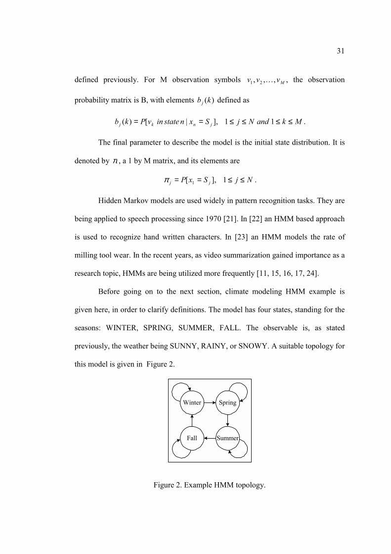
Before going on to the next section, climate modeling HMM example is
given here, in order to clarify definitions. The model has four states, standing for the
seasons: WINTER, SPRING, SUMMER, FALL. The observable is, as stated
previously, the weather being SUNNY, RAINY, or SNOWY. A suitable topology for
this model is given in Figure 2.
Winter Spring
SummerFall
Figure 2. Example HMM topology.

32
In addition to the transition probabilities )( ija depicted in the figure as
arrows, there are the observation probabilities )(kb j . Again, estimates can be made
regarding these probabilities. If it is assumed that measurements are made daily, the
transition probabilities between consecutive seasons would be about 3654 . Since no
transitions are allowed between non-consecutive seasons, self-transition probability
of a season to itself would be 365361 . Note that the topology of the model forces
season order.
Observation probability estimation would require long-term observation.
Most likely, depending on the climate, probability of snowy days in summer will be
very close to zero, rainy days will be most probable in spring and fall, and sunny
days will be scarce in winter. A possible distribution is given in Table 1. Note that
each column adds up to 1.
Table 1. Example HMM observation probabilities.
)(kb j j = WINTER j = SPRING j = SUMMER j = FALL k = SUNNY 0.1 0.3 0.7 0.3 k = RAINY 0.3 0.6 0.3 0.6 k = SNOWY 0.6 0.1 0.0 0.1
3.2 Basic Problems for Hidden Markov Models
Three problems are required to be solved for the HMMs to be useful in real-world
applications [21]:
Problem 1. The first problem is finding the probability that a given
observation sequence is generated by a given model. Given an observation sequence

33
ToooO l21= and a model ),,( πλ BA= , find )|( λOP , the probability of the
observation sequence.
Problem 2. Given an observation sequence ToooO l21= , and a model
),,( πλ BA= , find the state sequence TxxxX l21= that best “explains” the
observation sequence. Note that, apart from degenerate cases there is not a “correct”
state sequence to be found. This problem is involved with the hidden part of the
process being observed.
Problem 3. Adjust the model parameters ),,( πλ BA= so that )|( λOP is
maximized. This is the model training problem. The solution to his problem would
enable one to optimally tune the model to a given observation sequence.
3.3 Solution to Basic Problems of HMMs
3.3.1 Problem 1
A procedure known as the forward procedure is used for calculating the probability
of O given λ . First, forward variable )(inα is defined as the probability of the
partial state sequence until time n and state i , given the model λ .
)|,()( 21 λα iqoooPi nnn == �
Note that the probability being looked for is
∑=
=N
iT iOP
1)()|( αλ .
This probability can be found inductively.
Initialization: Niobi ii ≤≤= 1),()( 11 πα

34
Induction:
≤≤−≤≤
= +=
+ ∑ NjTt
obaij nj
N
iijnn 1
11),()()( 1
11 αα
Termination: ∑=
=N
iT iOP
1)()|( αλ
The induction step takes into account that state j can be reached from all
states, and calculates the probability of being in state j using ∑=
N
iijn ai
1)(α . The
multiplication with )( 1+nj ob adds observation 1+no into the picture. Recursion in
)(inα makes it possible to calculate ∑=
=)N
iT iOP
1)(|( αλ .
3.3.2 Problem 2
As stated before, a “correct” state sequence cannot be found for a given observation
sequence. Rather, an “optimal” sequence is sought for, with different definitions of
optimality. The most popular solution, the Viterbi algorithm finds the single best
state sequence as a whole [21], maximizing ),|( λOqP . In order to find this
probability, a definition should be made.
]|,,[max)( 21121,,, 121
λδ nnnqqqn oooiqqqqPin
��
�
== −−
.
Note that )(inδ is the highest probability among the probabilities of all single
paths, at time n , accounting for the first n observations and ending in state i.
)(inδ can also be written recursively as
MjTn
obaij njijnNin ≤≤≤≤
⋅= −≤≤ 11
),(])([max)( 11δδ .
Viterbi algorithm is implemented using )(inδ :

35
Initialization: Niobi ii ≤≤= 1),()( 11 πδ
0)(1 =iψ
Recursion: MjTn
obaij njijnNin ≤≤≤≤
⋅= −≤≤ 11
),(])([max)( 11δδ
NjTn
aij ijnNin ≤≤≤≤
= −≤≤ 12
],)([maxarg)( 11δψ
Termination: )]([max1
* iP TNiδ
≤≤=
)]([maxarg1
* iq TNiT δ≤≤
=
Backtracking: 1,,2,1),( *11
*h−−== ++ TTnqq nnn ψ
)(inψ is a matrix used for storage of most likely states at time 1−n that will
transition to state i at time n . In other words, it holds the argument that maximizes
)(1 jn+δ for all n and j.
3.3.3 Problem 3
Although the model parameters )π,,( BA that maximize the probability of an
observation sequence cannot be solved for analytically, there are iterative methods
that can locally maximize )λ|(OP . The Baum-Welch method is used in this work
[21].
First of all, the backward variable must be introduced. Similar to the forward
variable, backward variable )(inβ is the probability of observation sequence from
1+n to the end, being generated by the model λ , with state i when time is n :
),|()( 21 λβ iqoooPi nTnnn == ++ l
The probability of being in state i at time n is defined as
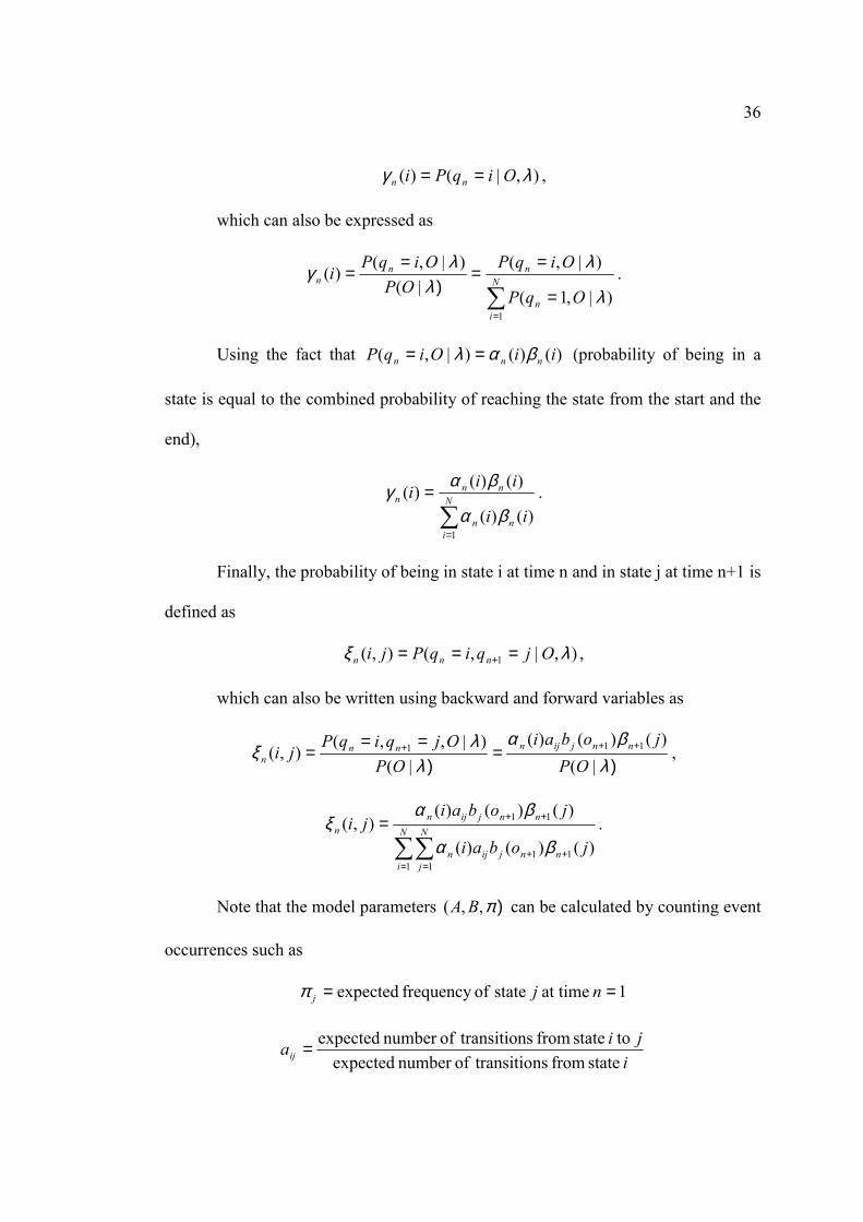
36
),|()( λγ OiqPi nn == ,
which can also be expressed as
∑=
=
==
)=
= N
in
nnn
OqP
OiqPOP
OiqPi
1)|,1(
)|,(|(
)|,()(
λ
λλ
λγ .
Using the fact that )()()|,( iiOiqP nnn βαλ == (probability of being in a
state is equal to the combined probability of reaching the state from the start and the
end),
∑=
= N
inn
nnn
ii
iii
1)()(
)()()(
βα
βαγ .
Finally, the probability of being in state i at time n and in state j at time n+1 is
defined as
),|,(),( 1 λξ OjqiqPji nnn === + ,
which can also be written using backward and forward variables as
)=
)==
= +++
λβα
λλξ
|()()()(
|()|,,(
),( 111
OPjobai
OPOjqiqPji nnjijnnn
n ,
∑∑= =
++
++= N
i
N
jnnjijn
nnjijnn
jobai
jobaiji
1 111
11
)()()(
)()()(),(
βα
βαξ .
Note that the model parameters )π,,( BA can be calculated by counting event
occurrences such as
1 at time state offrequency expected == njjπ
ijiaij state from ns transitioofnumber expected
to state from ns transitioofnumber expected=

37
jjv
kb kj statein timesofnumber expected
statein whilensobservatio ofnumber expected)( =
Also note that )(1 iγ is the probability of being in state i at time 1=n ,
∑=
T
nn ji
1),(ξ is the expected number of transitions from state i to state j , and
∑=
T
nn i
1)(γ is the expected number of times in state i . Using these, a set of re-
estimation formulas are defined [21]:
)(1 jj γπ =
∑
∑
=
== T
nn
T
nn
ij
i
jia
1
1
)(
),(
γ
ξ
∑
∑
=
==
= T
nn
T
von
n
j
i
i
kb kn
1
1
)(
)(
)(γ
γ
Starting with an initial model )= πλ ,,( BA and using it to compute new
model parameters ( )πBA=λ ,, , it is proven that either λ=λ , or
)|()|( λOPλOP > [21]. That is, either the new model is the same with the old
one, or it is a better estimation. Therefore, an iterative method to re-estimate model
parameters by using λ in place of λ until there is no “change” in the model is
feasible. This iterative re-estimation method gives a most likely estimate HMM.
Initial model selection is important, as the procedure converges to a local minimum
around the initial values.

38
CHAPTER 4
PROPOSED VIDEO SUMMARIZATION SYSTEM
4.1 Overview of the System
The proposed system consists of three stages, namely preprocessing, feature
extraction and decision making stages, as shown in Figure 3.
Figure 3. System Block Diagram.
Throughout the proposed system, video is processed shot by shot and
preprocessing stage handles shot boundary detection. Feature extraction stage
generates a feature vector for each shot, which is processed by decision making stage
in order to summarize the video.
Decision making stage is the 'intelligent' engine of the system. It uses hidden
Markov models (HMM) that take the feature vectors that are output in the feature
Feature Extraction Decision Making Pre-processing
AudioDecode &
Demux
Shot boundary detection
Audio classification
Face detection
Location change detection
Motion activity extraction
Training (Baum-Welch)
Segmentation (Viterbi)
Video
State sequence
Input Video

39
extraction stage as observation symbols. In an HMM, observable symbols are
assumed to be generated by an unobservable process. The HMM is a model of this
unobservable process, and by observing the HMM information about actual process
can be achieved. In the proposed system, the decision making stage treats the input
video as the unobservable process. Through extracting features, and modeling the
video by means of an HMM that is observing these features, the system segments the
input video into its scenes.
It has been pointed out in Chapter 2 that different video categories require
different summarization techniques. Similarly, the videos in the same category may
have different properties related to summarization. Different sub-categories of videos
may need different models, or different features may be useful in summarizing them.
For example, story-based videos are all based on a story, hence in order to
summarize them segments that tell an uninterrupted part of the story should be
identified. However, the method through which the story is conveyed changes
according to the type of the video (film, sitcom), genre of the video (musicals, action
films, dramas), and even to the director of the video.
A general method that takes all these factors into account and summarizes the
given video is not feasible to build. However, a framework system may be built
which can be adapted to the current input video. The first step in this adaptation is
the definition of content types.
4.2 Content Types
The problem of summarizing different kinds of video is solved by flexible behavior
of the decision making mechanism. Content types, classes of videos that can be

40
summarized using the same features and the same model, are defined. Videos
belonging to a content type, have some parallel properties that permit them to be
processed similarly in the context of video summarization. It should be noted that
content types are not genres or video types. A western series and a thriller movie can
have the same content type, while two comedy movies can belong to different
content types.
A set of features and an initial HMM can be associated with each content
type. In such an approach the features and the model are determined empirically.
Using different features and models allow the system to exploit production patterns
and content characteristics of each content type. By supplying content type
information, user is able to modify the behavior of the system.
Within the context of this thesis two content types are defined, and are
elaborated below.
4.2.1 Dialog-Driven Content
Dialog-driven content can be defined as the type of story-based videos that are made
up mainly of dialog scenes following each other to build a story. There may be action
scenes within the content, but dialog scenes are in dominance. The obvious examples
of this content type are situation comedies. Sitcoms are made up of shots of people
conversing in different rooms, with an occasional shot reserved for signaling location
or time changes. There are no action scenes, action is implied through conversations
and settings. The story is based on conversations and the humor contained within
them. Other examples of dialog-driven videos are dramas, and some other TV series.
Films usually are not dialog-driven.
41
In order to segment scenes in a dialog-driven video, a number of
characteristics can be exploited. Detecting location changes is useful, since scene
boundaries typically occur at points the location changes. Identification of shots that
do not belong to dialogs will be useful in catching time or location change shots.
Speech and human face existence information can be used to segment dialog as
shown in [17]. On the other hand, motion information will probably be useless, given
that all dialog scenes exhibit similar motion characteristics.
4.2.2 Action-Driven Content
Action-driven content is the type of story-driven content in which the story is told
through a mixture of dialog and action scenes. Dialog scenes are not as dominant as
they are in dialog-driven content. Action scenes have a significant role in moving the
story, and usually the final climax is solved in an action scene. In fact, action-driven
content may depend more on action scenes to tell a story than it depends on dialog
scenes. Cartoons are an example for this situation. All kinds of action movies, most
cartoons, and some TV series fall into this category.
Obviously, motion information is one of the required features to properly
identify dialog scenes (low motion) and action scenes (high motion). Location
change information is also useful, since location change usually implies scene
change.
4.3 Preprocessing
Preprocessing stage analyzes the video stream, and identifies shot boundaries. Since
all processing is achieved on the shots as the atomic unit, identification of the shot
42
boundaries is of utmost importance to the performance. An automatic method is used
to detect shot-boundaries, and results of this method are manually edited to further
refine the boundaries.
For shot boundary detection, an automatic method [10] works by clustering
frames of the video into two classes using the 2-means algorithm on a two-
dimensional feature space. The features are pixel difference and histogram difference
between consecutive frames. By applying 2-means clustering, the set of all frames is
segmented into boundary and non-boundary clusters.
In most cases this algorithm gives satisfactory results. However, when there
are complex shot transitions, such as wipes or long dissolves, or cut-resembling
events, such as flashes, the algorithm may fail to detect correct boundaries. Manual
editing is useful in such cases. Shot boundaries identified in this stage are used
throughout the whole system.
4.4 Feature Extraction Stage
The feature extraction stage analyzes preprocessed video and extracts the necessary
features for each shot in the video. Output of this stage is a sequence of feature
vectors, one feature vector for each shot in the video.
A maximum of 4 features are extracted for each shot: Face existence, audio
class, location change existence and motion activity level. It is important to note that
not all of the features may be extracted at all times. Features to be extracted are
selected according to the content type of the video.

43
Some fundamental low-level features are standardized in MPEG-7. The
feature extractors use the face, color histogram, motion activity and audio
parameters, as descriptors from MPEG-7 [25].
4.4.1 Face Detection
Presence of human faces in video is an important clue in summarization. Action or
dialog shots usually contain faces, whereas establishing shots seldom do. Scenes
usually start and end with establishing shots, which are wide-angle views serving as
the introduction or conclusion of the scene.
Face detection is quite a mature topic with diverse solutions [26]. Many
methods employ techniques depending on isolating skin color regions in the input
image, which provide a good initial estimate for the face regions, since the human
skin color occupies a narrow region in any 3-D color space. The method used in the
system applies a set of heuristic rules on color skin regions in order to detect faces
[17].
Temporally regular spaced sample frames are taken from each shot, and
connected regions of skin color in YUV color space are searched. Following table
lists the boundaries of the skin-color region YUV space.
Table 2. Skin color region boundaries.
Skin-color bounds
Magnitude (Min.)
Magnitude (Max)
Angle (Min)
Angle (Max)
UV-space 0 100 130 170 YV-space 0 200 0 40 UY-space 0 200 225 260
44
The following set of geometric heuristics are also applied to each connected
region of skin color:
• Area: The area of a connected face region should be less than a quarter, and
more than 0.004 times the frame area. This heuristic eliminates extremely
large or very small regions.
• Aspect Ratio: A connected face region should have an aspect ratio between
0.9 and 1.7. This heuristic eliminates some undesired regions with unexpected
shapes.
• Location: A connected face region should be located entirely in the upper
three quarters of the frame, without having any pixels closer to the sides more
than 1/8 of frame width. Aesthetically, an important human face is not placed
near the bottom or the sides of the frame [6]. This heuristic eliminates regions
that do not obey this rule.
• 'Fullness': Fullness is the ratio of the area of the connected face region to the
area of the bounding rectangle of the connected region. The sides of a
bounding rectangle are defined to be parallel to that of frames. A connected
region should have a 'fullness' value more than 1/4. This heuristic eliminates
strangely shaped regions, particularly crescent and tree shapes, which occur
frequently but cannot be eliminated by the other heuristics.
If at least one connected skin color region passes all the heuristics defined
above, the frame is assumed to have a face. If at least one frame in a shot has a face,

45
than that shot is decided to be a FACE shot. All other shots are labeled as NOFACE
shots.
4.4.2 Audio Analysis
Audio track contains a wealth of information relevant to the content of the video.
Speech, sound effects, environmental sounds and even music can provide clues about
the content. Humans can easily understand the occurring events in a movie by only
listening to the audio track, merging the information they gather from dialogs, sound
effects (e.g. gunshots, footsteps), environmental sounds (e.g. the sounds of a busy
street) and music (e.g. creepy music when tension rises). Moreover, one can even
keep track of events in action scenes, where speech is scarce, using other auditory
clues.
The audio track can be used to aid in the process of automatic video
summarization. A semantically high-level understanding of the audio signal (e.g.
speaker identification, topic detection, scene segmentation) would enhance
summarization performance considerably, but it is costly to reach such high-level
semantics.
On the other hand, low-level properties of the audio track (e.g. short-time
energy, fundamental frequency), which are less costly to extract, can improve
summarization performance significantly, if carefully utilized [14, 17]. For example,
in a typical soccer match the volume of sound increases when an important event
takes place. In such a case, local energy of the sound signal can be thresholded to
identify high-volume segments and used in sports content summarization [14].

46
Moreover, a number of low-level features can be merged together to reach a
higher semantic description of the audio track. For example, in [27], the authors
propose a method that utilizes energy, fundamental frequency and zero crossing rate
of the signal to detect silence, noise, music and speech segments. Similar higher level
descriptions of the audio segments can then be used in video segmentation.
In the proposed system audio content of each shot is determined using a
method based on the method in [27]. Digitized content of each shot is divided into
frames of constant length. Each frame is first analyzed to detect silent frames. Non-
silent frames are then separated into speech and music categories [27]. A biased
voting mechanism is then used to classify each shot into one of the classes
SILENCE, MUSIC or SPEECH.
Reasoning behind this method is the possibility of modeling an audio signal
as a linear combination of 4 signals (silence s[n], speech v[n], music v[n] and noise
q[n]) [27]:
[ ] ][][][ nqanvansana qvs ++=
Furthermore, the different characteristics of each signal can be summarized as
follows [27]:
• Silence signals contain a quasi-stationary background noise, with an energy
level lower than that of other signals.
• Speech signals contain voiced, unvoiced and plosive signals.
• Music signals are composed of sounds with 'peculiar' characteristics of
periodicity.
• Noise signals are all signals that do not belong to the other categories.

47
Silence Detection
Each audio frame's energy is calculated according to the frame energy equation.
∑∈
=nframeif
iaN
nE 2])[(1][
Nf is the number of samples in a frame, and a[i] is the digital audio signal.
Dividing the sum by number of samples in the frame is for normalization. E(n) for
each frame n is compared with a threshold, Ts to determine whether the frame is a
silence frame or not. The threshold Ts is calculated using a buffer of silence frames
using the same method as calculating frame energies.
∑=
=bufferN
oibuffers nb
NT 2])[(1
The buffer contains Nbuffer samples. Initially, the buffer is filled the first
frames of the shot, which are assumed to be silent. As the frames are being
processed, detected silence frames are inserted to the buffer replacing the oldest
frames. Thus, the threshold is adjusted to changing silence levels within a shot.
In order to incorporate contextual information, a finite state machine (FSM)
with K+1 states is used (see Figure 4). Using the contextual information enables the
system to reject isolated frames. These frames are either low-energy frames within a
high-energy sequence of frames, or vice versa; caused by momentary silences or
noise.

48
Figure 4. Finite state machine with K+1 states.
The first state in FSM, state 0, is the silence state, and state K is the non-
silence state. All other states are 'inner states'. FSM is initially at state 0. After
calculating each audio frame's energy and comparing with the current silence
threshold of the shot, FSM moves one state higher; otherwise FSM moves one state
lower. Frames that belong to inner states are not classified until a silence or non-
silence state is reached. They are then classified according to the state reached [27].
Non-Silence Classification
After silence detection, non-silence frames are further analyzed to be classified into
speech, music or noise. During this analysis, periodicity properties and zero crossing
rates (ZCR) of frames are used, according to the following principles:
• Speech is composed of three classes of sounds: Unvoiced, voiced and plosive
sounds.
• Unvoiced sounds have a low signal energy, no pitch and high frequency.
• Voiced sounds have greater signal energy than unvoiced sounds, and they
exhibit periodicity over short intervals of time.
• Plosive sounds are transient with high energy levels, and they have no pitch.
• Music segments have a wider frequency range than speech segments.
state0
state1
state K
… sil
non-sil non-sil non-sil
sil sil sil
non-sil

49
• Music segments usually show periodicity characteristics with fundamental
periods greater than that of voiced speech segments.
During the analysis, periodic frames are identified and, if the fundamental
period falls within the fundamental period of typical music frames, they are labeled
as music. Non-periodic frames are assumed to be noise. ZCR rate analysis of
periodic non-music frames decides, if they are speech, music or noise.
Periodicity and fundamental frequency analysis of frames are achieved by
taking autocorrelations of frames. Since the autocorrelation function can be thought
to measure “shifted similarity”, if the signal is quasi-periodic, the autocorrelation
function has a significant local maximum on the fundamental period of the signal.
Based on this concept, the autocorrelation function, ],[ knNϕ , is used to derive a
periodicity measure [27]. ],[ knNϕ is defined as
∑∞
−∞==−++−=
ifN lNnnkiwkianiwiakn ,][][][][],[ϕ
where ][nw is a binary window:
−≤≤
=.,010,1
][otherwise
Nnnw f
The periodicity measure is
]0,[],[][ 0 nknnAN ϕϕ=
0k is the index at which the first significant local maximum occurs (the
fundamental period), and ]0,[nϕ is the value of autocorrelation function at zero.
Therefore, ][nAN is a measure of the 'strength' of the first peak. Note that for

50
periodic signals, ][nAN has a value of 1. The autocorrelation function always has a
maximum at 0, since a signal is identical to itself. All frames whose periodicity
measure falls above an empirically selected threshold are classified as periodic.
Periodic frames, whose fundamental period falls between the expected range
of the fundamental periods of music segments, are classified as music. The rest are
speech candidates. Non-periodic frames are labeled as noise.
Zero crossing rate analysis is performed to classify speech candidate
segments. Since speech segments are made up of voiced (periodic), unvoiced (non-
periodic) and plosive (non-periodic) sounds, any speech candidate frame is
concatenated with its non-silent, non-music neighbors. Analysis is made on this
concatenation.
In a typical speech signal, the ZCR is expected to vary more than that of a
typical music signal due to unvoiced and plosive, high-frequency sounds. For every
speech candidate, its and its concatenated neighbors' zero crossing rates are
calculated using the formula
∑∈−
∈
+⋅−=nframei
nframeif
iaiaN
nZCR1
1])[]1[sgn(21)(
If the ZCR variance of the concatenated block is above an empirically
determined threshold for speech segments, all concatenated frames are classified as
speech frames. Otherwise, they are classified as music, if they are periodic, and as
noise if they are not.
Finally, after each segment in a shot are classified into one of the classes
silence, speech, music, or noise, a simple voting is performed among the segment
results to obtain a single class for the shot, speech, music, noise or silence.

51
4.4.3 Location Change Analysis
Usually, a scene takes place in a single location. In a typical dialog scene, the
director first introduces the viewer to the scene, the location and the people, by
means of an 'establishing shot' [6]. An establishing shot usually provides a wide-
angle view of the location. After the establishing shot, alternating views of the
protagonists are shown as they converse. Shots of objects and places related to the
conversation, or wide-angle shots of the location may be interleaved among these
alternating views. The scene may be finalized by another wide-angle shot.
An action scene is similarly introduced, but the progression of shots in a
scene is not as organized as in a dialog scene. Moreover, action scenes are less likely
to take place in a single location and the single location may not be easily detectable
in some cases. Consider a fight scene in a warehouse, or a gunfight in the main street
of a Wild West town. Alternating shots will show different parts of the setting that
are semantically linked, but have no low-level visual clue that they are actually in the
same location.
Due to the complexity of detecting location changes in action scenes, the
proposed approach attempts to identify location changes in dialog scenes and simpler
action scenes.
The problem is approached by a windowed histogram comparison method. A
fixed number of equally spaced frames are selected from each shot as samples. Color
histograms of sample n, nh , is calculated by
∑∈
=imageyx
n cyxBch),(
),,()(
where ),,( cyxB is a function that returns if the pixel at (x,y) is of color c.

52
A discrete temporal window, Wl, is defined. The window contains a fixed
number, N, of samples. At each iteration of the algorithm, mean and variance
histograms of the samples within the window are calculated. As a result of this
operation a mean histogram, which has the mean value of each color for samples
within Wl, and a variance histogram, which holds the variance of each color, are
obtained.
∑−+
=
=1
)(1)(Nn
niim ch
Nch
∑−+
=
−=1
2))()((1)(Nn
nimiv chch
Nch
Mean histogram mh and variance histogram vh are used to determine if the
sample in front of the window, Nnh + is similar to the ones in the window. D1
distance of histograms, absolute differences of color buckets, is used as a difference
measure.
)()()( chchcD NnmNn ++ −=
This difference value is compared with product of the variance matrix and a
threshold ( locT ). If the difference is larger than locv Tch ⋅)( for any color, sample
Nn + is labeled as a location change sample. Otherwise, it is a non location change
sample (see Figure 5). The window is moved one sample forward, and if there are
more samples available, the algorithm is iterated.

53
Shot 1 Shot 2 Shot 3 Shot 4 Shot 5 Shot 6
WL (N = 3)
h2(c) h3(c) h4(c)
c c c c cc
h1(c) h5(c) h6(c)
hv(c)
c
hm(c)
c
... ...
......
Figure 5. Location change detection method.
After labeling each sample, simple voting is applied between samples from
each shot to determine the shot's label. If the total number of location samples is
more than the number of non location change samples, the shot is labeled as a
location change shot. Number of samples taken from each shot, window size Wl, and
threshold locT are empirically determined.
4.4.4 Motion Activity Analysis
There are two general types of motion in video. The first one is global motion,
motion of the scene as a whole. The second is object motion, motion of objects in the
scene, in such a way that can be identified from global motion. Global motion is
generally caused by camera motion, such as panning and zooming. Object motion is
also called motion activity.
Amount of object motion is an important feature in video summarization.
Intuitively, it is expected that there should be more object motion in action scenes

54
when compared to dialog scenes. Objective of this feature extractor is to obtain a
qualitative measure of object motion in each shot.
In order to obtain the motion information in one frame of the video, block
matching motion estimation algorithm can be used [28]. The frame, fN, is divided
into fixed size blocks, typically 8 pixels by 8 pixels. For each block bn a search is
made to find the most similar area in the next frame, fN+1, of the video. The whole
frame fN+1 is not searched; only a square area around the original position of the
block bn is checked, which is the search window Ws. Starting from the original
position, all possible positions within Ws are evaluated according to a similarity
measure, and the most similar position is assumed to be the position to where the
pixels in fN have moved to [28]. The similarity is decided by taking differences of the
values of the pixels and summing their absolute value.
In order to obtain a quantitative measure for motion activity in each frame,
variance of the magnitudes of all motion vectors in frame fN is calculated [29]. Note
that, by taking variance of motion vectors, one gets rid of most global motion that
might be present in the frame. Through averaging motion activity values of all
frames, motion activity value for the shot can be obtained. Finally, value for each
shot is quantized into five levels, as suggested by the MPEG 7 standard [25].
4.5 Decision Making Stage
The decision making mechanism uses hidden Markov models to model the input
video. Two different approaches are implemented for decision making. The first
approach models the entire video using a hidden Markov model, whereas the second
one models different types of scenes with different hidden Markov models.

55
In both cases, HMMs take the extracted features as observation symbols.
States of HMMs correspond to shot types, as in dialog shot, non-dialog shot, high
action shot and establishing shot and state transitions are assumed to be made at shot
boundaries. Note that observation symbols are expected to have different observation
probabilities in different states. For example, human faces are more likely to appear
in dialogue shots rather than non-dialogue shots. Topologies, transition probabilities
and observation probabilities of initial HMMs are determined so that they reflect
actual video and scene structure.
The first approach to video summarization is based on identifying the type of
each shot and detecting scene boundaries based on these shot types. A single HMM
is used to label each shot in the video.
The second approach, however, identifies the scenes directly. Different types
of scenes are modeled by different HMMs. The decision making mechanism tries to
recognize both scene boundaries and the model that has the highest likelihood of
having produced the observation symbols within the scene.
4.6 Models
Models for the first mode of analysis are built to represent entire videos. However,
different models are used for different content types. This is expected to make the
summarization system to adapt itself to the input video and produce better
summarization performance. Three initial models are built for content type
dependent video summarization. They use different features and have different
topologies (see Figure 6). The features each model uses is explained in Section 5.2.

56
Figure 6. HMMs used in content type dependent video summarization. (D: Dialogue, ND: Non-dialogue, LA: Low-action, HA: High-action, T: Transition, A: Action, DT:
Dialogue transition, AT: Action Transition)
For the second mode of analysis, video summarization based on scene
modeling, HMMs represent individual scenes. Two basic initial HMMs are built; one
for dialog scenes, the other for action scenes. Both HMMs are ergodic two state
HMMs.
The dialog scene model uses
• Audio class,
• Face existence,
• Location change
features. Speech and face are the basic elements of a dialog, and thus the initial
dialog scene model has a high likelihood of speech and face existence. Music and
noise have lower observation probabilities, since dialogue scenes have dominant
speech content [6]. One of the two states is selected to represent the establishing
shot. Location changes have a higher probability of occurring in that shot, and face
existence has a lower probability.
The action scene model uses
(b)
ND/HAD/LA T
(c)
AT DT
D A
(a)
NDD

57
• Audio class,
• Motion activity
features. The audio class feature is used solely to distinguish action scenes, which
typically have much less speech content when compared to dialog scenes.
Observation probability of speech in the action scene model is low compared to
music and noise, which are prominent characteristics of action scenes. Motion
activity is used to implement the notion of establishing shot in an action scene.
Establishing shots in action scenes tend to have lower motion content, when
compared to action shots [6]. One of the states in the model is again chosen to
represent the establishing shot. It should be noted that low motion shots might also
appear during the course of the action scene unrelated to scene establishment [6].
All models’ initial probabilities are defined based on the experience of the
author and they are further trained to obtain better modeling. This training process is
explained in the following section.
4.7 Training
HMM training has well-defined solutions [21], and the models in the system are
trained using the well known Baum-Welch algorithm, which is explained in Section
3.4. However, the selection of the samples with which models are trained needs
special attention. In video summarization, the usual approach is to train an HMM by
other videos similar to the test video [11, 15, 16, 17, 24].
The approach taken for training in the first mode of operation, however, is
slightly different. Before segmentation, each model is trained by the test video itself.
The rationale behind this approach may be understood by recalling that each content
58
type has an HMM that models the videos belonging to that content type, and that
videos having the same content types have differences that may be relevant for
summarization. For example, all action-driven videos are understood to be built up of
dialog and action scenes. However, the frequency of action scenes, length of dialog
scenes, usage of the camera, lighting, and sound, and many other properties are
bound to be different in different action-driven videos. These differences are related
to the script, the acting, the directing and the editing of the video and therefore they
are unavoidable.
Note that these differences can also be modeled by HMMs. The frequency of
action scenes, for example, is modeled by the transition probability from dialog shots
to action shots. The length of dialog scenes corresponds to self-transition probability
of a dialog shot. Usage of the camera changes the way the motion activity feature is
interpreted. Scenes that are shot closer to the subject tend to have higher motion
activity values than wide-angle scenes. This and other feature related differences are
related to observation probabilities in an HMM.
Fortunately, a trained HMM is able to capture these differences and adapt
itself to the movie. Through self-training the movie, models are able to capture the
properties that are different among videos that belong to the same content type. This,
in addition to good content type models, allows better modeling of the underlying
process by which the video is generated, and thus provides a better performance. In
fact, this process itself may not be called “training”, but simply a model “tuning”. As
a result, better video models can be obtained.

59
In order to obtain better scene models, however, the usual approach is
adopted. Initial scene models are trained with the observation sequences of sample
scenes, and five scene models are obtained, two for each scene type.

60
CHAPTER 5
SIMULATIONS
Throughout the simulations a test set comprised of segments from four videos are
used. All videos are recorded from Turkish Radio and Television (TRT) with an off-
the-shelf PCI MPEG-1 encoder card. Two of the videos are Hollywood family
movies, and belong to action-driven content type. The other two are Turkish-made
serials belonging to dialogue-driven content type.
Parts that are not related to the story, such as commercial breaks, summaries
of previous episodes, and credit sequences, are removed from each video. These
parts have different structures and properties when compared to the rest of the video;
commercials, for example, have much different auditory properties and camera
usage. Likewise, summaries are often constructed by combining a few shots from
each scene in the previous episode, in effect compressing the scene structure. Since
they do not belong in the structure of the story, non-story parts of videos fall outside
the scope of this study, and hence are not included in simulations.
Simulations are conducted in three phases. In the first phase, performance of
the first video summarization method is evaluated. The second phase elaborates
performance of the other method, which uses the likelihood values to classify the

61
scenes in predetermined durations and the final phase compares these two
approaches against the clustering based video summarization approach explained in
[18].
In the first two phases, videos first have their shot boundaries identified by
the automatic algorithm. After the boundaries are refined by an operator, necessary
feature extractors are used to generate feature vectors for each shot. These feature
vectors are fed to the decision making mechanism which produces shot type labels.
Produced labels are processed one final time to get the result: scene structure of the
video.
Scene structure is compared with a manually obtained ground truth scene
structure, and precision and recall values are calculated as quantitative performance
measures. Precision is defined as the ratio of the number of correctly identified
scenes to the number of all identified scenes and recall is defined as the ratio of the
number of correctly identified scenes to the number of scenes in the ground truth.
5.1 Feature Extractor Performance Simulations
Before examining video summarization simulations, performance of the feature
extractors are briefly presented. Outputs of all four feature extractors are compared
with subjective ground truth data from the test set. Table 3 shows results in terms of
percentage of the shots correctly classified. Note that relatively simple feature
extractors are used in the system in order to have less computational complexity.

62
Table 3. Feature extractor performance
Feature Serial A Serial B Movie A Movie B Overall Face 86.3% 83.0% 76.1% 56.4% 75.5%
Audio 75.5% 79.2% 71.8% 71.2% 74.4% Location Change 88.2% 94.3% 85.6% 76.1% 86.1% Motion Activity 100% 88.7% 72.9% 91.4% 88.3%
5.2 Content Type Simulations
In the first phase of the simulations, all videos in the test set are analyzed using
different hidden Markov Models and feature sets. This analysis is done in order to
evaluate performances of different models and features with different content types.
First of all, audio and face features are used to segment the video into
dialogue and non-dialogue shots. More than 2-state topologies are not used, since
more state (scene) types do not have any semantic meaning. The results (Table 4)
indicate that audio and face features alone are not successful in segmentation of the
sample set. Closer examination of the results reveals that the videos are highly under-
segmented.

63
Table 4. Recall / precision values for different HMM topologies using audio and face features.
Audio, face Recall / precision 2-state
Dialog driven 0.139 / 1.000 Action driven 0.450 / 1.000
The next experiment adds the location change feature to the system, and this
time 3- and 4-state topologies are used as well, since location changes imply
transitions. The results in Table 5 show that dialog driven content is segmented quite
well with this set of features, using the 2-state topology. Generally, dialog driven
content is better segmented than action driven content with this feature set.
Table 5. Recall / precision values for different HMM topologies using audio, face and location change features.
Audio, face, location change Recall / precision 2-state 3-state 4-state
Dialog driven 1.000 / 0.742 0.778 / 0.489 0.584 / 0.548 Action driven 0.741 / 0.784 0.584 / 0.438 0.800 / 0.648
After adding the motion activity feature to the observation set, the
performance decreases (Table 6). Scenes are observed to be over-segmented,
although dialog driven content still has better results.
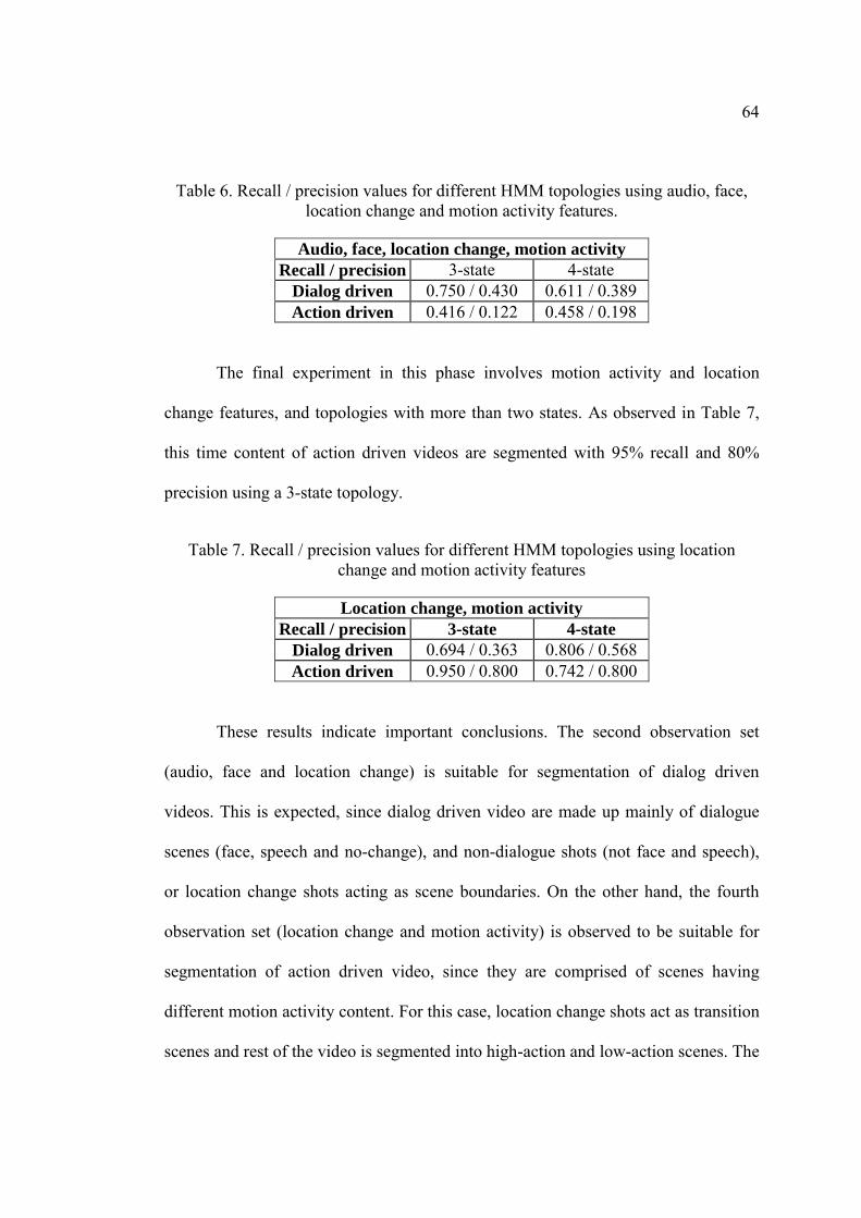
64
Table 6. Recall / precision values for different HMM topologies using audio, face, location change and motion activity features.
Audio, face, location change, motion activity Recall / precision 3-state 4-state
Dialog driven 0.750 / 0.430 0.611 / 0.389 Action driven 0.416 / 0.122 0.458 / 0.198
The final experiment in this phase involves motion activity and location
change features, and topologies with more than two states. As observed in Table 7,
this time content of action driven videos are segmented with 95% recall and 80%
precision using a 3-state topology.
Table 7. Recall / precision values for different HMM topologies using location change and motion activity features
Location change, motion activity Recall / precision 3-state 4-state
Dialog driven 0.694 / 0.363 0.806 / 0.568 Action driven 0.950 / 0.800 0.742 / 0.800
These results indicate important conclusions. The second observation set
(audio, face and location change) is suitable for segmentation of dialog driven
videos. This is expected, since dialog driven video are made up mainly of dialogue
scenes (face, speech and no-change), and non-dialogue shots (not face and speech),
or location change shots acting as scene boundaries. On the other hand, the fourth
observation set (location change and motion activity) is observed to be suitable for
segmentation of action driven video, since they are comprised of scenes having
different motion activity content. For this case, location change shots act as transition
scenes and rest of the video is segmented into high-action and low-action scenes. The

65
final point to emphasize is utilization of all features for segmentation degrades
performance.
(a)
(b)
Figure 7. Sample simulation results a) Dialog driven, b) Action driven. Consecutive scenes are colored differently; the actual colors (black or white) are irrelevant.
Figure 7 shows two sample results from both content types. Video sequences
are segmented into their scenes. The graphs show consecutive scenes in different
Ground Truth
00:00 02:53 05:46 08:38 11:31
Result
00:00 02:53 05:46 08:38 11:31
Ground Truth
00:00 02:53 05:46 08:38 11:31 14:24 17:17
Result
00:00 02:53 05:46 08:38 11:31 14:24 17:17

66
colors. Scene boundaries (i.e. points at which colors change) are relevant, colors of
individual scenes should not necessarily match between results and ground turth.
5.3 Scene Modeling Simulations
Second phase of simulations investigates the feasibility of modeling scenes for video
summarization. Observation sequence input to the decision making module is
divided into partitions of a fixed number of shots and each partition’s likelihood of
being created by each model is calculated. The model that has the highest likelihood
is then used to segment that partition, and get shot labels.
Remember that five scene models are used in the system (see Section 4.6).
Three of these models are dialog scene models and two are action scene models.
Table 8 and Table 9 list precision and recall values for the partitions being classified
correctly by dialog and action scene models, respectively. During this analysis, the
actual class of a partition (i.e. ground truth) is determined by voting among its shots.
If the number of shots belonging to action scenes are more than the number of shots
belonging to dialog scenes, the partition is assumed to be an ‘action partition.’ A
‘dialog partition’ is defined similarly.
Table 8. Dialog scene precision and recall.
Precision / Recall Serial A Serial B Movie A Movie B Overall 100 0 / 0 1.00 / 1.00 1.00 / 1.00 1.00 / 0.50 0.75 / 0.6350 1.00 / 0.25 1.00 / 1.00 1.00 / 1.00 1.00 / 0.33 1.00 / 0.6525 1.00 / 0.57 1.00 / 0.94 0.82 / 1.00 0.85 / 0.75 0.92 / 0.81
Part
ition
si
ze
10 1.00 / 0.53 1.00 / 0.89 0.90 / 0.90 0.84 / 0.76 0.93 / 0.77
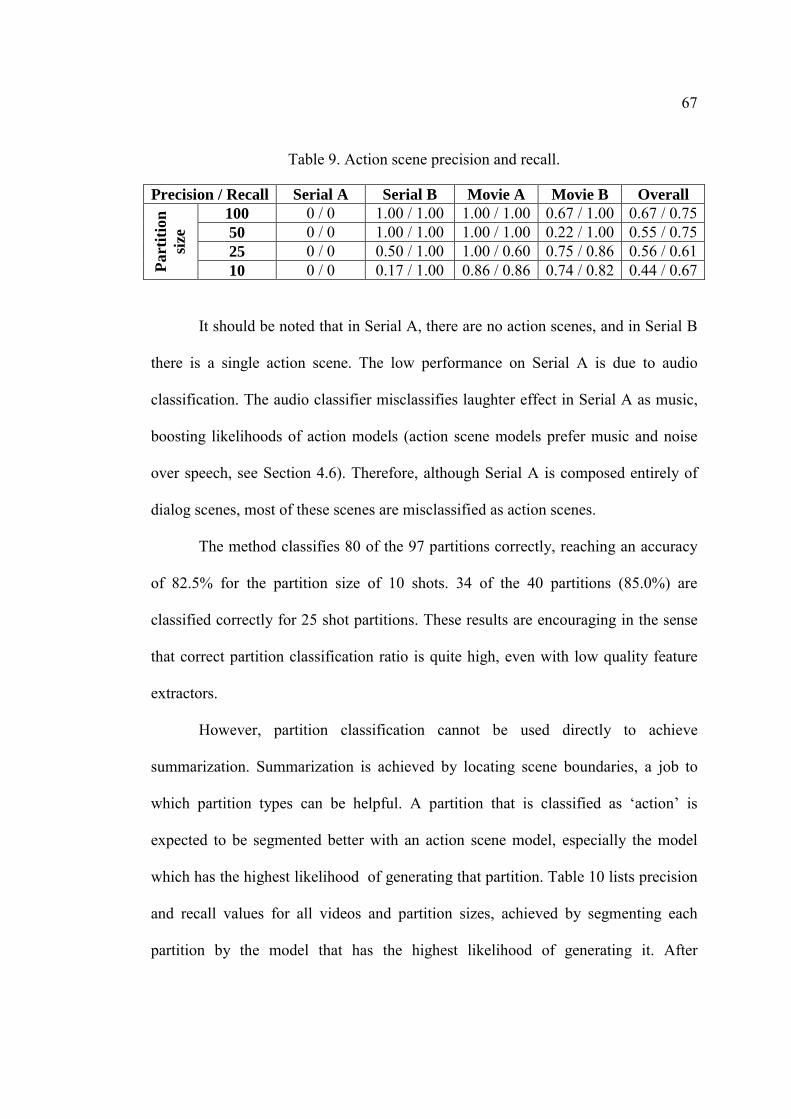
67
Table 9. Action scene precision and recall.
Precision / Recall Serial A Serial B Movie A Movie B Overall 100 0 / 0 1.00 / 1.00 1.00 / 1.00 0.67 / 1.00 0.67 / 0.7550 0 / 0 1.00 / 1.00 1.00 / 1.00 0.22 / 1.00 0.55 / 0.7525 0 / 0 0.50 / 1.00 1.00 / 0.60 0.75 / 0.86 0.56 / 0.61
Part
ition
si
ze
10 0 / 0 0.17 / 1.00 0.86 / 0.86 0.74 / 0.82 0.44 / 0.67
It should be noted that in Serial A, there are no action scenes, and in Serial B
there is a single action scene. The low performance on Serial A is due to audio
classification. The audio classifier misclassifies laughter effect in Serial A as music,
boosting likelihoods of action models (action scene models prefer music and noise
over speech, see Section 4.6). Therefore, although Serial A is composed entirely of
dialog scenes, most of these scenes are misclassified as action scenes.
The method classifies 80 of the 97 partitions correctly, reaching an accuracy
of 82.5% for the partition size of 10 shots. 34 of the 40 partitions (85.0%) are
classified correctly for 25 shot partitions. These results are encouraging in the sense
that correct partition classification ratio is quite high, even with low quality feature
extractors.
However, partition classification cannot be used directly to achieve
summarization. Summarization is achieved by locating scene boundaries, a job to
which partition types can be helpful. A partition that is classified as ‘action’ is
expected to be segmented better with an action scene model, especially the model
which has the highest likelihood of generating that partition. Table 10 lists precision
and recall values for all videos and partition sizes, achieved by segmenting each
partition by the model that has the highest likelihood of generating it. After

68
likelihood calculation and before Viterbi segmentation the model is trained with
partition observation sequence for “tuning” (see Section 4.7).
Table 10. Precision and recall table for segmentation using scene models.
Precision / Recall Serial A Serial B Movie A Movie B Overall 100 0 / 0 0.50 / 0.33 0.60 / 0.33 0.43 / 0.25 0.38 / 0.2350 0 / 0 0.60 / 0.50 0.15 / 0.56 0.57 / 0.33 0.33 / 0.3525 0.75 / 0.43 0.15 / 0.40 0.17 / 0.44 0.23 / 0.27 0.33 / 0.39
Part
ition
si
ze
10 1.00 / 0.20 0.06 / 0.20 0.05 / 0.20 0.41 / 0.75 0.38 / 0.34
Low performance with Serial A is due to most of its partitions being
classified wrong (see Table 8 and Table 9). The overall lack of performance is
related to the partitioning method. Partitions are determined without any regard to the
structure of input video. Therefore, a partition can have shots belonging to different
scenes, and those scenes can be of different types. On the other hand, while
segmenting partitions, all shots within a partition are assumed to belong to the same
scene. A partition is segmented by a model which is trained on single-scene data. As
a result, segmentation of partitions using scene models fails to reach the performance
level of content type dependent video segmentation.
5.4 Comparison With Deterministic Approach
The performance of “semantic-level table of content construction technique” [18] is
shown in Table 5. For the HMM-based method, the best performances for different
content types are tabulated. For Type I content, audio, face and location change
features are used with 2-state HMM topology, whereas for Type II content, location
change and motion activity features on 3-state topology are utilized. Best performing
scene modeling result (25 shot-long partition) is also given.

69
Table 11. Rule-Based vs. best performance HMM results
Recall / precision
Deterministic [18]
HMM for Dialog driven
HMM for Action driven
Scene Modeling
Dialog driven 0.806 / 0.410 1.000 / 0.742 0.694 / 0.363 0.450 / 0.415Action driven 0.734 / 0.764 0.741 / 0.784 0.950 / 0.800 0.200 / 0.355
5.5 Evaluation of the Results
Results of content type simulations show that different models and feature sets are
needed to better summarize different content types. This result is line with the
definition of content types defined in Chapter 4, namely that different content types
need different models and features for summarization. Better summarization is
achieved by using a summarization scheme that takes the content types into account.
Scene modeling simulations suggest that classification of ‘partitions’ of
videos can feasibly be achieved by scene HMMs. However, identification of scene
boundaries, which is a prerequisite for video summarization, is not possible by the
proposed method. It is understood that, in order to increase performance, a method
that can determine both partition boundaries and partition types should be developed.
Finally, comparison of these three methods show that content type dependent
video summarization method outperforms deterministic method for both content
types. Using different models for different content types is due to the flexibility of
HMM-based strategy, which is not possible for deterministic approaches. It is seen
that scene modeling based method is not as competitive as the other methods.

70
CHAPTER 6
CONCLUSIONS
Story-based video summarization is an attractive research field with promising
application areas. Shot level video summarization has attained a certain maturity.
Scene level summarization, which aims to identify story segments in a story based
video, is the natural summarization method and it is desired over shot level
summarization; since it generates concise summaries, more similar to the way
humans summarize a video. Unfortunately, unlike shot level summarization, which
can be handled through processing low-level features only, scene level
summarization requires combining semantically low-level features to reach higher-
level semantic concepts.
Diversity of production techniques further complicate the problem.
‘Production,’ as defined in Chapter 2, is the process by which a story is transformed
into a video. Different types of video, as in sitcoms and movies, are produced
differently. Director’s and editor’s choices affect production as well. Moreover,
video production industry has developed conventions that guide a director or editor
in building the video. While summarizing story based videos, the differences and
similarities in production should be taken into account.

71
In this thesis an automatic HMM based video segmentation system is
presented. In the system, each video is analyzed to get four low-level features: face
detection, audio classification, location change detection and motion activity. A
feature vector for each shots of the input video is created with the results of the
analysis. A decision making stage processes the feature vector sequence and assigns
shot type labels to every shot. Hidden Markov models are used in the decision
making stage.
Two different methods to video summarization are implemented. The first
method uses a single hidden Markov model to segment the entire video. In order to
account for different production techniques the system is configured according to
content types. Two content types; dialog driven and action driven, are defined within
this thesis. Content type dictates the particular features and model to be used in the
system. The ability to adapt to the content type being analyzed is one of the core
features of the system.
The model chosen for summarization of a video is trained with features of
that video before summarization. This makes use of the HMM’s capability to model
video properties that are not dictated by the content type; the ones that are related to
director’s choices, such as camera usage and scene length. Together with the content
type adaptation, self-training enables the system to fine tune itself to its input. The
need for using different models and features for the two content types is
demonstrated by experiments.
For the second approach, the scenes instead of videos, are modeled by the
decision making hidden Markov models. After feature extraction, the feature vector
sequence is divided into fixed length partitions. For each partition, all models are

72
tried, and the one that gives the highest likelihood of generating the partition is
selected as the representative model of that partition. Partitions are then segmented
with their representative models, after self-training. Partition summaries are
combined to get a video summary. Identifying scene types is central to this approach.
Finally, proposed methods are compared against a clustering based video
summarization method [18]. Content type dependent video summarization method
enjoys the highest performance, and scene identification based method is the least
successful method.
Dialog driven and action driven content types do not span all story based
videos. More content types can be defined as an improvement to the system.
Enlarging the scope of the system to non-story based videos is another option. In
order to obtain a full-fledged video summarization system, more sophisticated
feature extractors that have higher performance can be used.
On the other hand, a technique that identifies scene types and segments scene
boundaries can be developed. Scene identification of the second method suggests
that such a technique could enhance performance.

73
REFERENCES
[1] The Internet Movie Database, http://www.imdb.com.
[2] Dyne:bolic, http://dynebolic.org.
[3] M. R. Naphade and T. S. Huang, “Extracting Semantics From Audiovisual Content: The Final Frontier in Multimedia Retrieval,” IEEE Trans. on Neural Networks, vol.13, no. 4, pp. 793-810 July 2002.
[4] J. V. Mascelli, H. Gür (transl.), “Sinemanın 5 Temel Öğesi,” İmge Kitabevi Yayınları, 2002.
[5] B. T. Truong, S. Venkatesh and C. Dorai, “Scene Extraction in Motion Pictures,” IEEE Trans. on Circuits and Systems for Video Technology, vol. 13, no. 1, pp. 5-15, January 2003.
[6] D. Arijon, “Grammar of the Film Language,” Silman-James Press, 1991.
[8] F. Germeys, “Film Perception,” http://www.psy.kuleuven.ac.be/labexppsy/ top/ filipweb/ research2.htm.
[7] C. Dorai and S. Venkatesh, “Computational Media Aesthetics: Finding Meaning Beautiful,” IEEE Multimedia, The Media Impact Column, vol. 8, no. 4, pp. 10-12, October-December 2001.
[9] R. Lienhart, “Comparison of Automatic Shot Boundary Detection Algorithms,” Proc. Image and Video Processing VII, 1999.
[10] M. R. Naphade, R. Mehrotra, A. M. Ferman, J. Warnick, T. S. Huang, A. M. Tekalp, "A High Performance Algorithm For Shot Boundary Detection Using Multiple Cues," IEEE International Conference on Image Processing 1998, 1998.
[11] A. M. Ferman, A. M. Tekalp, “Probabilistic Analysis and Extraction of Video Content,” IEEE International Conference on Image Processing 1999, 1999.

74
[12] M. R. Naphade, I. V. Kozintsev, T. S. Huang, “A Factor Graph Framework for Semantic Video Indexing,” IEEE Trans. on Circuits and Systems for Video Technology, vol. 12, no. 1, pp. 40-52, January 2003.
[13] L. Chen, M. T. Özsu, “Rule-Based Scene Extraction From Video,” Proc. of IEEE International Conference on Image Processing 2002, vol. 2, pp. 737-740, 2002.
[14] R. Leonardi, P. Migliorati, “Semantic Indexing of Sports Program Sequences by Audio-Visual Analysis,” to appear in IEEE International Conference on Image Processing 2003, September 2003.
[15] P. Chang, M. Han, Y. Gong, “Extract Highlights from Baseball Game Video With Hidden Markov Models,” Proc. of IEEE International Conference on Image Processing 2002, vol. 1, pp. 609-612, 2002.
[16] T. Liu, J. R. Kender, “A HMM Approach to the Structure of Documentaries,” IEEE Workshop on Content-based Access of Image and Video Libraries 2000, pp. 111-115, 2000.
[17] A. A. Alatan, A. N. Akansu, W. Wolf, “Multi-Modal Dialogue Scene Detection using Hidden Markov Models for Content-based Multimedia Indexing”. Int. Journal on Multimedia Tools and Applications, Kluwer Ac., 2001.
[18] Y. Rui, T. S. Huang, S. Mehrotra, “Constructing Table-of-Content for Videos,” Multimedia Systems, Special section on Video Libraries 7, pp. 359-368, 1999.
[19] J. Pearl, “Probabilistic Reasoning in Intelligent Systems: Networks of Plausible Inference,” Morgan Kaufmann Publishers, 1998.
[20] A. Papoulis, S. U. Pillai, “Probability, Random Variables and Stochastic Processes,” McGraw-Hill, 4th ed., 2002.
[21] L. R. Rabiner, “A Tutorial on Hidden Markov Models and Selected Applications in Speech Recognition,” Proceedings of the IEEE, vol. 77, no. 2, pp. 257-286, February 1989.
[22] H.-S. Park, B.-K. Sin, J. Moon, S.-W. Lee, “A 2-D HMM Method for Offline Handwritten Character Recognition,” International Journal of Pattern Recognition and Artificial Intelligence, vol. 15, no. 1, pp. 91-105, 2001.
[23] R. K. Fish, M. Ostendorf, G. D. Bernard, D. A. Castañon, “Multilevel Classification of Milling Tool Wear with Confidence Estimation,” IEEE Transactions on Pattern Analysis and Machine Intelligence, vol. 23, no. 1, pp. 75-85, January 2003.
75
[24] L. Xie, S-F Chang, A. Divakaran, H. Sun, “Structure Analysis of Soccer Video With Hidden Markov Models,” Proc. of IEEE International Conference on Acoustics, Speech, and Signal Processing 2002, vol. 4, pp. 1096-1099, May 2002.
[25] B. S. Manjunath, P. Salembier, T. Sikora, “Introduction to MPEG-7,” John Wiley & Sons Ltd., 2002.
[26] M.-H. Yang, D. J. Kreigman, N. Ahuja, “Detecting Faces in Images,” IEEE Transactions on Pattern Analysis and Machine Intelligence, Vol. 24, pp. 34-58, 2002.
[27] C. Saraceno, R. Leonardi, “Identification of Story Units in Audio-Visual Sequences by Joint Audio and Video Processing,” Proc. of IEEE International Conference on Image Processing 1998, pp. 363-367, 1998.
[28] A. M. Tekalp, “Digital Video Processing,” Prentice Hall Signal Processing Press, 1995.
[29] K. A. Peker, A. Divakaran, T. V. Papathomas, “Automatic Measurement of Intensity of Motion Activity of Video Segments,” SPIE Conference on Storage and Retrieval for Media Databases, vol. 4315, pp. 341-351, 2001.