Multi-level thresholding using quantum inspired meta ... · PDF fileMulti-level thresholding using quantum inspired meta-heuristics ... Ant Colony Optimization, Quantum Inspired Simulated

Knowledge-Based Systems 67 (2014) 373–400

Contents lists available at ScienceDirect

Knowledge-Based Systems

journal homepage: www.elsevier .com/ locate /knosys

Multi-level thresholding using quantum inspired meta-heuristics

http://dx.doi.org/10.1016/j.knosys.2014.04.0060950-7051/� 2014 Elsevier B.V. All rights reserved.

⇑ Corresponding authors. Address: Department of Computer Science & Engineer-ing, Jadavpur University, Kolkata 700032, India (I. Saha).

E-mail addresses: [email protected] (I. Saha), [email protected] (S. Bhattacharyya).

1 Both the authors are joint first authors and contributed equally.

Sandip Dey a,1, Indrajit Saha b,c,⇑,1, Siddhartha Bhattacharyya d,*, Ujjwal Maulik b

a Department of Information Technology, Camellia Institute of Technology, Madhyamgram, Kolkata 700129, Indiab Department of Computer Science & Engineering, Jadavpur University, Kolkata 700032, Indiac Institute of Informatics, University of Wroclaw, Wroclaw 50383, Polandd Department of Information Technology, RCC Institute of Information Technology, Beliaghata, Kolkata 700015, India

a r t i c l e i n f o

Article history:Received 9 October 2013Received in revised form 3 March 2014Accepted 6 April 2014Available online 14 May 2014

Keywords:Image segmentationMultilevel thresholdingOtsu’s methodQuantum computingStatistical test

a b s t r a c t

Image thresholding is well accepted and one of the most imperative practices to accomplish image seg-mentation. This has been widely studied over the past few decades. However, as the multi-level thres-holding computationally takes more time when level increases, hence, in this article, quantummechanism is used to propose six different quantum inspired meta-heuristic methods for performingmulti-level thresholding faster. The proposed methods are Quantum Inspired Genetic Algorithm, Quan-tum Inspired Particle Swarm Optimization, Quantum Inspired Differential Evolution, Quantum InspiredAnt Colony Optimization, Quantum Inspired Simulated Annealing and Quantum Inspired Tabu Search.As a sequel to the proposed methods, we have also conducted experiments with the two-Stage multi-threshold Otsu method, maximum tsallis entropy thresholding, the modified bacterial foraging algo-rithm, the classical particle swarm optimization and the classical genetic algorithm. The effectivenessof the proposed methods is demonstrated on fifteen images at the different level of thresholds quantita-tively and visually. Thereafter, the results of six quantum meta-heuristic methods are considered to cre-ate consensus results. Finally, statistical test, called Friedman test, is conducted to judge the superiority ofa method among them. Quantum Inspired Particle Swarm Optimization is found to be superior amongthe proposed six quantum meta-heuristic methods and the other five methods are used for comparison.A Friedman test again conducted between the Quantum Inspired Particle Swarm Optimization and all theother methods to justify the statistical superiority. Finally, the computational complexities of the pro-posed methods have been elucidated for the sake of finding out the time efficiency of the proposedmethods.

� 2014 Elsevier B.V. All rights reserved.

1. Introduction

Image thresholding can be recognized as the easiest and mostefficient method that is widely used for image segmentation. Thisis used as an effective tool to bifurcate images into object and back-ground [1]. For its first kind, the pixel intensities of the image aregrouped into two classes, called bi-level image thresholding. Whilethe number of groups exceed two, it is recognized as multi-levelthresholding [2]. Both of them can be identified by acclimatizingparametric or nonparametric approaches [3,4]. Moreover, thereexists different algorithms for bi-level image thresholding thatcan also be extended to their corresponding multi-level versions,

if necessary [2,5]. When the level increases in multi-level thres-holding, the number of computations increase as well. This couldadd significant difficulties specially when higher level thresholdvalues are evaluated. Many algorithms have been proposed so farthat can handle this situation efficiently, where some of them aredeveloped for a specific purpose. These algorithms have theirown advantages and disadvantages. However, in this paper, sixnew quantum meta-heuristic methods for multi-level thresholdingare presented that can be used efficiently for general purpose.

Generally a wave function, jwi which exists in Hilbert space, isemployed for describing a quantum system. The Schrödinger equa-tion (SE) is assumed to be accountable for overseeing the inherentdynamism of quantum computing (QC). A quantum bit or qubit isconsidered as the smallest unit for a two-state quantum machine.The qubit may be in ‘‘0’’ state or in ‘‘1’’ state or even in superposi-

tion between these two states where, j0i ¼ 10

� �and j1i ¼ 0

1

� �. The

superposition of the two state vectors are symbolized by the

http://crossmark.crossref.org/dialog/?doi=10.1016/j.knosys.2014.04.006&domain=pdf

http://dx.doi.org/10.1016/j.knosys.2014.04.006

mailto:[email protected]




http://www.sciencedirect.com/science/journal/09507051

http://www.elsevier.com/locate/knosys

374 S. Dey et al. / Knowledge-Based Systems 67 (2014) 373–400

equation jwi ¼ aj0i þ bj1i where, a; b are complex numbers satis-

fying the equation jaj2 þ jbj2 ¼ 1. Coherence in QC exists whenthe states are in superposed form maintaining a constant phaserelationship between them. When the coherence is forced to bedestroyed, decoherence occurs. For decoherence, the requisite

probability for collapsing to the state j1i and j0i are jaj2 and jbj2,respectively. Quantum entanglement is a fascinating feature inquantum system that can be employed to describe the correlationsbetween the diversified qubits [6,7]. Quantum entanglement of aquantum state can be demonstrated using the density matrix[6,7]. Entanglement can be analyzed, distorted, and even washedout, if required, [6,8]. Quantum interference is an another interest-ing feature of a quantum system. The advancement of newresearch era advocates the researchers to entrench the algorithmicconstruction of different quantum-inspired evolutionary algo-rithms (QIEA) by incorporating the philosophy of quantum system[9]. So far, a number of combinatorial optimization problems havebeen resolved using QIEA, where the concept of wave interferencewas introduced [8]. Han et al. designed an QIEA where the qubitwith some probability constraints, linear superposition betweenstates and various Q-gates for population assortment have beenused [9].

Nowadays, meta-heuristic approaches are widely used invarious domains of engineering and science. Many authors haveutilized different meta-heuristic approaches for image threshold-ing. Some distinctive applications of meta-heuristic are given in[10–14]. Mostly, the traditional approaches of multi-level thres-holding for gray scale images use binary encoding scheme, whereeach pixel is represented by 8 bits. Thus, the length of the stringincreases in multiply of 8 for higher levels. As this article is con-fined on gray scale images, this fact motivated us to propose analternative technique based on quantum inspired meta-heuristicmethods for multi-level thresholding using the notion of qubits,where real value encoding scheme is used to determine the activepixel. For this purpose,

ffiffiffiLp

number of random pixels are selected,where, L represents the maximum pixel intensity value of the grayscale test image. With this encoding scheme, Quantum InspiredGenetic Algorithm (QIGA), Quantum Inspired Particle Swarm Opti-mization (QIPSO), Quantum Inspired Differential Evolution (QIDE),Quantum Inspired Ant Colony Optimization (QIACO), QuantumInspired Simulated Annealing (QISA) and Quantum Inspired TabuSearch (QITS) for multilevel thresholding are proposed. The effec-tiveness of these methods is demonstrated on fifteen images atthe different level of thresholds in terms of different quantitativemeasures. Thereafter, consensus results of these six methods arealso computed. Finally, statistical test, called Friedman test[15,16], is conducted to judge the superiority of a method amongthem.

As a part of comparative study to adjudge the efficacy of theproposed quantum inspired methods, we have resorted to fiveclassical algorithms viz., Two-Stage Multithreshold Otsu method(TSMO) [17], Maximum Tsallis entropy Thresholding (MTT)2 [18],Modified Bacterial Foraging (MBF) algorithm [19], classical ParticleSwarm Optimization for multi-level thresholding [20] and classicalGenetic Algorithm for multi-level thresholding [21]. The compara-tive study reveals that the Quantum Inspired Particle Swarm Optimi-zation outperforms the proposed five quantum meta-heuristicmethods and the other five classical algorithms used for comparison.

2. Background

The field of quantum computing became popular since thenotion of quantum mechanical system was anticipated at the early

2 As abbreviated in [18].

1980s [22]. The aforesaid quantum mechanical machine is able tosolve some particular computational problems awfully efficiently[23]. In [24], the author has recognized that classical computerfaces lack of ability while simulating quantum mechanical system.The author has presented a structural framework to build quantumcomputer. Alfares et al. analyzed how the notion of quantum algo-rithms can be applied to solve some typical engineering optimiza-tion problems [25]. According to their perception, some problemsmay arise when the features of QC are applied. These problemscan be avoided by using certain kind of algorithms. Hogg has pre-sented a framework for structured quantum search where Groversalgorithm was applied to correlate the cost with the gate’s behav-ior [26]. In [27], the authors have extended the work and proposeda new quantum version of combinatorial optimization. Rylanderet al. presented a quantum version of genetic algorithm wherethe quantum principles like superposition and entanglement wereemployed on modified genetic algorithm. In [28], Moore et al. pro-posed a framework for general quantum-inspired algorithms.Later, Han et al. [9] developed an evolution algorithm which wasapplied for solving knapsack problem. In their paper, basic quan-tum principles like qubits and rotation quantum gate were used.Afterward, in [9], the authors have designed another version ofquantum inspired evolutionary algorithm by Han et al. where theperformance was evaluated according to the angles of the rotationgates and later, in [29], a new improved version of this algorithmwas presented. They divided the evolution stage into two differentphases and proposed alteration to the quantum gate adding a ter-mination criterion. The improved version of the work presented in[9] was proposed by Zhang et al. where they applied a differentapproach to get the best solution [30]. Narayan et al. presented agenetic algorithm where quantum mechanics was used for modifi-cation of crossover scheme [31]. Moreover, Li et al. developed amodified genetic algorithm using quantum probability representa-tion. They adjusted crossover and mutation processes for attainingthe quantum representation [32]. In [33], the authors presented aquantum-inspired neural network algorithm where also the basicquantum principles were employed to symbolize the problemvariables.

The instinctive compilation of information science with thequantum mechanics resort to construct the concept of quantumcomputing. Quantum evolutionary algorithm (QEA) was admiredas a probability based optimization technique. It uses qubitsencoded strings for its quantum computation paradigm. The intrin-sic principles of QEA help to facilitate for maintaining the equilib-rium between exploitation and exploration. In recent years, someresearchers have presented some QEAs to solve particular combi-natorial optimization problems. A typical example of QEA is Filterdesign by Zhang et al. [34]. The researches are still going on tocreate purposeful and scalable quantum computers.

Meta-heuristic optimization techniques are employed heuristi-cally in searching algorithms. They use iterative approach to havebetter solution by fleeing from local optima. So they coerce somebasic heuristic to compensate from local optima. There are somerenowned Meta-heuristic techniques namely, GA, PSO, DE, ACO,SA and TS which are applied for optimization with different man-ners. Holland has proposed genetic algorithms (GAs) which imper-sonate the belief of some natural fruition. GAs can be appliedefficiently in data mining for classification. In 2006, Jiao et al. pre-sented organizational coevolutionary algorithm for classification(OCEC) [35]. In OCEC, bottom-up searching technique has beenadopted and enthused from the coevolutionary model that can effi-ciently knob multi-class learning. Kennedy and Eberhart first pro-posed Particle Swarm Optimization (PSO) in 1995 inspiring fromthe synchronized movement in flocks of birds [36]. In PSO, thepopulation of particle is the particle swarm. In 2004, Sousa et al.projected PSO in data mining [37]. PSO can be skilfully used in

S. Dey et al. / Knowledge-Based Systems 67 (2014) 373–400 375

rule based searching process. In recent years, many researchershave tried to improve the performance of PSO and proposed vari-ous alternatives of PSO. In [38], the authors presented algorithmon parameters settings. Some authors have furnished their effortsfor the betterment and variation of PSO by combining diversetechniques [39–41].

The actions of ant colonies are governed by heuristic algorithmsuch as Ant colony optimization (ACO) [62] . In 2002, Parpinelliet al. proposed the concepts of Ant-Miner based ACO for generatingthe classification rules [42]. Subsequently, Sousa et al. presented aPSO/ACO algorithm, hybrid in nature, to discover classificationrules [37]. The working principle of PSO/ACO is divided in twophases. In its first part, ACO determines a rule surrounding onlythe ostensible attributes and in later part, PSO determines the rulepotentially comprehensive with incessant attributes. In [43], somefacts on quantum dots (QDs) have been reported.

Stron and Price presented the differential algorithm (DE) in1997. This is a population-based stochastic meta-heuristic optimi-zation technique. DE has proved its excellence in float-point searchspace. There are numerous modified versions of DE algorithmsinvented so far; most of them are built to solve continuous optimi-zation problems. But it has low efficacy to solve discrete optimiza-tion problems and faces several problems such as engineeringrelated problem especially for routing or scheduling or even com-binational type problems. Binary DE, AMDE [44] presented in 2006by Pampara et al. that can solve numerous numerical optimization.

In [45], a coalesce form of simulated annealing and geneticalgorithm (SA–GA) has been proposed by Fengjie et al. The authorshave employed 2D Otsu algorithm in low contrast images. Theiralgorithm can differentiate the ice-covered cables from its back-grounds. Luo et al. have also presented an combined (SA–GA) algo-rithm for colony image segmentation in [46]. According to Luoet al., the collective gives a better result because the individualshortcomings have been eliminated in the proposed algorithm. In[47], SA and improved Snake model based algorithm were pre-sented by Tang et al. in image segmentation. In [48], Nakib et al.presented a research work on non-supervised image segmentationbased on multi-objective optimization. In addition to this theyhave developed another alternative of SA that can able to resolvethe histogram Gaussian curve fitting problem. The details are givenin [48]. Yufei et al. have worked on image segmentation. They havecombined image entropy and SA together and presented a segmen-tation algorithm. According to their research work, the segmenta-tion process can speed up the contours evaluation. Apart from that,the combination of this meta-heuristic approach can cause forterminating the contours evolution automatically to appositeboundaries [49]. In another paper, Garrido et al. have presentedSA based segmentation approach based on MRI for left ventricle.The details were presented in [50]. Zhijun et al. used a combinedapproach of GA and SA in image segmentation to find thresholdvalue for image segmentation [34].

In 1997, tabu search was first proposed by Fred Glover to allowhill climbing to surmount from local optima [51]. The man behinddrafting the basic ideas for tabu search is Hansen [2]. Later, supple-mentary research has been carried out about this meta-heuristicapproach that was reported in Glover [52,53]. There are manycomputational experiments that establish the completeness andefficacy as a meta-heuristic approach. Faigle et al. and Fox alsoinvestigated the theoretical facets of tabu search that have beenreported in [54,55], respectively. Huang et al. have developed analgorithm called Two-Stage Multithreshold Otsu method (TSMO)to improve the effectiveness of Otsu’s method [17]. Zhang et al.presented a Maximum Tsallis entropy Thresholding method(MTT) for image segmentation. They have employed TsallisEntropy using Artificial Bee Colony Approach for optimization[18]. In 2011, Sathya et al. have proposed another multi-level

thresholding algorithm for image segmentation based on histo-gram called Modified Bacterial Foraging (MBF) algorithm [19].

2.1. Brief highlights of image thresholding methods

Sezgin and Sankur presented an extensive and comprehensivestudy on image thresholding. The details have been presented intheir survey paper [56]. They have classified these methods intosix groups as described below.

� Histogram shape-based methods.� Clustering-based methods.� Entropy-based methods.� Object attribute-based methods.� Spatial methods.� Local methods.

In the first category, some histogram’s property like peaks, val-leys and curvatures are taken into consideration. In the second cat-egory, the gray-level pixels are grouped and clustered into twodivisions; one as foreground and other as background. In [56],the authors have described different cluster based methods by dif-ferent researchers in details. In entropy-based methods, entropy ofthe background and foreground areas is calculated. In some othermethods of this category, cross-entropy of the original image andits corresponding binary version is determined and later opti-mized. For object attribute-based methods, similarities like fuzzyshape similarity, edge coincidence and other various parametersof gray level image and its binary version are investigated. In thenext category, different statistical measures like probability distri-bution of higher-order and the correlation between pixels are ana-lyzed. Finally, local image characteristics are acclimatized todetermine its optimum threshold value. The details of variousmethods of each category are elaborately discussed by Sezginet al. in [56].

3. Otsu’s method for image thresholding

In multi-level thresholding, the original image is segregatedinto K number of classes. There are K � 1 thresholds namely,fh1; h2; . . . ; hK�1g, which are employed as separators between theconsecutive classes. The classes are assumed to beC1;C2; . . . ;Ck; . . . ;CK and the ranges of threshold values in theseclasses are ½0;1; . . . ; h1�; ½h1 þ 1; . . . ; h2�; . . . ; ½hk�1 þ 1; . . . ; hk�; . . . ;

½hK�1 þ 1; . . . ; L� 1� where, L is the maximum pixel intensity valueof the gray scale image.

In this research paper, one cluster based thresholding methodhas been exercised as an objective function. This method wasproposed by Otsu [57]. This is one of the most eminentthresholding method that is frequently used for image segmenta-tion [57]. The method finds a set of optimal thresholdsfh1; h2; . . . ; hK�1g that maximizes the between-class variance Ugiven by [57]

U ¼ #2fðh1; h2; . . . ; hK�1g ¼XK

i¼1

xiðli � lÞ ð1Þ

where K denotes the number of thresholds to be determined fromthe class C ¼ fC1;C2; . . . ;CKg and 0 6 h1 6 � � � 6 hK�1 < L. Here,

xi ¼Xj2Ci

pj; pj ¼ nj=N and li ¼Xj2Ci

jpj=xi ð2Þ

where nj signifies the number of pixels of an image measured at thejth intensity level and N is the total number of pixels intensities ofthe corresponding image. The probability of jth pixel of the image isdenoted by pj. xi is the probability of class Ci whereas, li represents


the mean of this class. l is known as the mean of class C. Note that,the number of optimum thresholds are determined by maximizingU [57].

4. Basics of quantum computing

The basic physical principles of quantum physics are used inquantum computer (QC) for information processing [7]. Schröding-er’s equation has been incorporated to rule over the mechanism ofquantum system. The state of any quantum mechanical system,jwi, which subsists in Hilbert space, can be considered as a vectordefined in a complex vector space. Let us assume that there existsset of vectors fj/ig; / ¼ 0;1; . . . ;Q� 1 where, the maximum valueof Q may be 1, which form an orthonormal basis for the vectorspace defined above, then jwi can be expressed as

jwi ¼X

/

c/j/i ð3Þ

where, c/ are complex coefficients satisfyingP

/jc/j2 ¼ 1. The‘‘bra-ket’’ notation is very popular and important as well in quan-tum mechanics. The ‘‘ket’’ vector, j�i is equivalent to a column vectorwhereas, its Hermitian conjugate or sometimes called complex con-jugate transpose, ‘‘bra’’ is denoted by h�j. The ‘‘bracket’’ is appearedto be h�j�i [7], which is formed by uniting the above two vectors.

In QC, the basic element of any two-state quantum system iscalled qubit. qubit is generally represented either by the ‘‘groundstate’’, j0i or by ‘‘excited state’’, j1i, which are basically normalizedand mutually orthogonal to each other. It can also be representedby the linear superposition of the basic states as jwi ¼ caaþ cbb

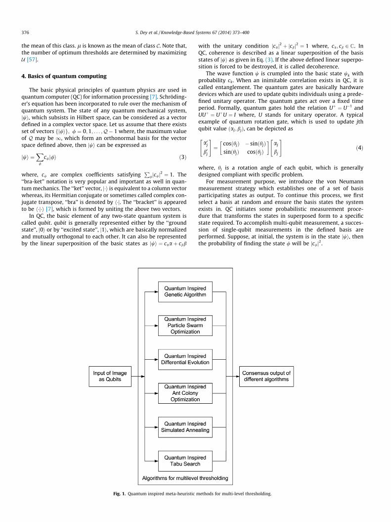
Fig. 1. Quantum inspired meta-heuristic m

with the unitary condition jcaj2 þ jcbj2 ¼ 1 where, ca; cb 2 C. InQC, coherence is described as a linear superposition of the basisstates of jwi as given in Eq. (3). If the above defined linear superpo-sition is forced to be destroyed, it is called decoherence.

The wave function w is crumpled into the basic state wk withprobability ck. When an inimitable correlation exists in QC, it iscalled entanglement. The quantum gates are basically hardwaredevices which are used to update qubits individuals using a prede-fined unitary operator. The quantum gates act over a fixed timeperiod. Formally, quantum gates hold the relation Uþ ¼ U�1 andUUþ ¼ UþU ¼ I where, U stands for unitary operator. A typicalexample of quantum rotation gate, which is used to update jthqubit value ðaj; bjÞ, can be depicted as

a0jb0j

" #¼

cosðhjÞ � sinðhjÞsinðhjÞ cosðhjÞ

� � aj

bj

" #ð4Þ

where, hj is a rotation angle of each qubit, which is generallydesigned compliant with specific problem.

For measurement purpose, we introduce the von Neumannmeasurement strategy which establishes one of a set of basisparticipating states as output. To continue this process, we firstselect a basis at random and ensure the basis states the systemexists in. QC initiates some probabilistic measurement proce-dure that transforms the states in superposed form to a specificstate required. To accomplish multi-qubit measurement, a succes-sion of single-qubit measurements in the defined basis areperformed. Suppose, at initial, the system is in the state jwi, thenthe probability of finding the state / will be jc/j2.

ethods for multi-level thresholding.


5. Proposed quantum inspired meta-heuristic methods formulti-level thresholding

In this section, six different quantum inspired meta-heuristicmethods are presented (see Fig. 1). Each method is described elab-orately in the subsections given below.

5.1. Quantum Inspired Genetic Algorithm

In this subsection, the authors have tied up the genetic algo-rithm, a meta-heuristic optimization technique with quantumprinciples to develop a new Quantum Inspired Genetic Algorithmfor multi-level thresholding (QIGA). The proposed QIGA is depictedin Algorithm 1. The details of QIGA is described in different subsec-tions given below.

5.1.1. Population generationThis is the initial part of the proposed QIGA. Here, a number of

qubit encoded chromosomes are employed to generate an initialpopulation. Initially, a n� L matrix is formed using two superposedquantum states, as given below [8]

jwi ¼

a11jw1i þ b11jw2ia12jw1i þ b12jw2i � � �a1Ljw1i þ b1Ljw2ia21jw1i þ b21jw2ia22jw1i þ b22jw2i � � �a2Ljw1i þ b2Ljw2i� � � � � � � � � � � � � � � � � � � � � � � � � � � � � � � � � � � � � � � � � � � � � � � � � � � � � �� an1jw1i þ bn1jw2ian2jw1i þ bn2jw2i � � �anLjw1i þ bnLjw2i

26666664

37777775ð5Þ

Algorithm 1. Steps of QIGA for multi-level thresholding

Input: Number of Generation: MxGenSize of the Population: VCrossover probability: Pcr

Mutation probability: Pm

No. of thresholds: K

Output: Optimal threshold values: h

1: Selection of pixel values randomly to generate V numberof initial chromosomes (POP) where length of eachchromosome is L ¼

ffiffiffiLp

, where, L represents maximumgray value of a selected image.

2: Using the concept of qubits to assign real value between(0,1) to each pixel encoded in POP. Let it produces POP0.

3: Using quantum rotation gate as given in Eq. (4), updatePOP0.

4: POP0 undergoes quantum orthogonality to generate POP00.5: Finding K number of thresholds as pixel values from each

chromosome in POP. It should satisfy the conditiongreater than ð>Þ randð0;1Þwith its corresponding value inPOP00. Let it gives POP�.

6: Compute fitness of each of chromosome in POP� using Eq. (1).7: Record the best chromosome b 2 POP00 and its threshold

values in TB 2 POP�.8: Apply tournament selection strategy to replenish the

chromosome pool.9: repeat

10: Select two chromosomes, k and m at random from ½1;V�where k – m.

11: if (randð0;1Þ < Pcr) then12: Select a random position, pos 2 ½1;L�.13: Perform crossover operation between two

chromosomes, k and m at the position pos.

14: end if15: until the pool of chromosomes are filled up16: for all k 2 POP00 do17: for For all position in k do18: if (randð0;1Þ < Pm) then19: Flip the corresponding position with random real

number.20: end if21: end for22: end for23: Repeat steps 3, 4 and 5.24: Save the best chromosome in c 2 POP00 and its

corresponding threshold values in TB 2 POP00.25: Compare the fitness value of the chromosomes of

b and c.26: Store the best chromosome in b 2 POP00 and its

corresponding threshold values in TB 2 POP00 (elitism).27: Repeat steps 8 to 26 for fixed number of generations,

MxGen.28: Report the optimal threshold values, h ¼ TB.

Here, jaijj2 and jbijj2 are the probabilities to find the state jw1i

and jw2i, respectively where, i ¼ 1;2; . . . ;n; j ¼ 1;2; . . . ; L and Lrepresents the maximum pixel intensity value of the input grayscale image. Each row in Eq. (5) signifies qubit representation ofa single chromosome. This is the possible scheme for encoding par-ticipating chromosomes for required number of solution usingsuperposition principle. jw1i and jw2i represent ‘‘0’’ state and ‘‘1’’state, respectively where jw1i þ jw2i is the superposition of thesetwo states for a two state quantum computing.

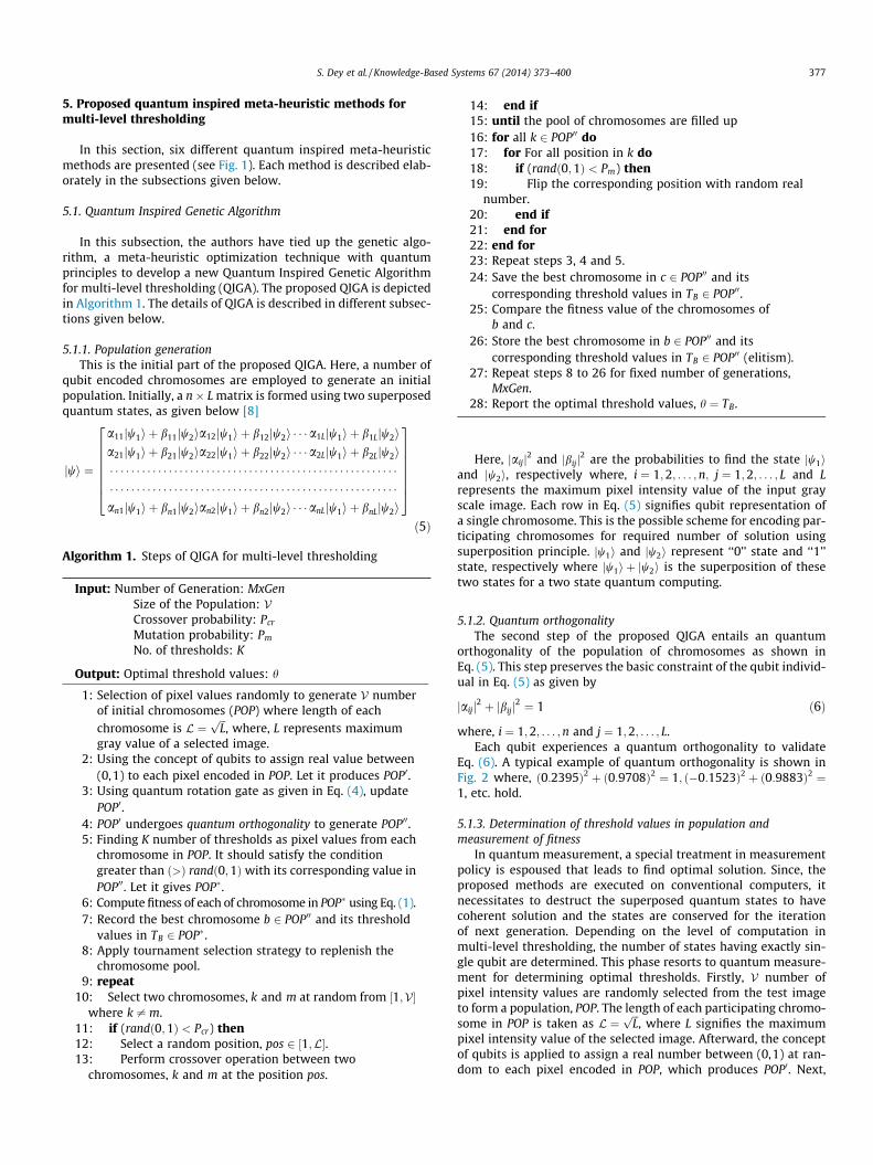
5.1.2. Quantum orthogonalityThe second step of the proposed QIGA entails an quantum

orthogonality of the population of chromosomes as shown inEq. (5). This step preserves the basic constraint of the qubit individ-ual in Eq. (5) as given by

jaijj2 þ jbijj2 ¼ 1 ð6Þ

where, i ¼ 1;2; . . . ; n and j ¼ 1;2; . . . ; L.Each qubit experiences a quantum orthogonality to validate

Eq. (6). A typical example of quantum orthogonality is shown inFig. 2 where, ð0:2395Þ2 þ ð0:9708Þ2 ¼ 1; ð�0:1523Þ2 þ ð0:9883Þ2 ¼1, etc. hold.

5.1.3. Determination of threshold values in population andmeasurement of fitness

In quantum measurement, a special treatment in measurementpolicy is espoused that leads to find optimal solution. Since, theproposed methods are executed on conventional computers, itnecessitates to destruct the superposed quantum states to havecoherent solution and the states are conserved for the iterationof next generation. Depending on the level of computation inmulti-level thresholding, the number of states having exactly sin-gle qubit are determined. This phase resorts to quantum measure-ment for determining optimal thresholds. Firstly, V number ofpixel intensity values are randomly selected from the test imageto form a population, POP. The length of each participating chromo-some in POP is taken as L ¼

ffiffiffiLp

, where L signifies the maximumpixel intensity value of the selected image. Afterward, the conceptof qubits is applied to assign a real number between (0,1) at ran-dom to each pixel encoded in POP, which produces POP0. Next,

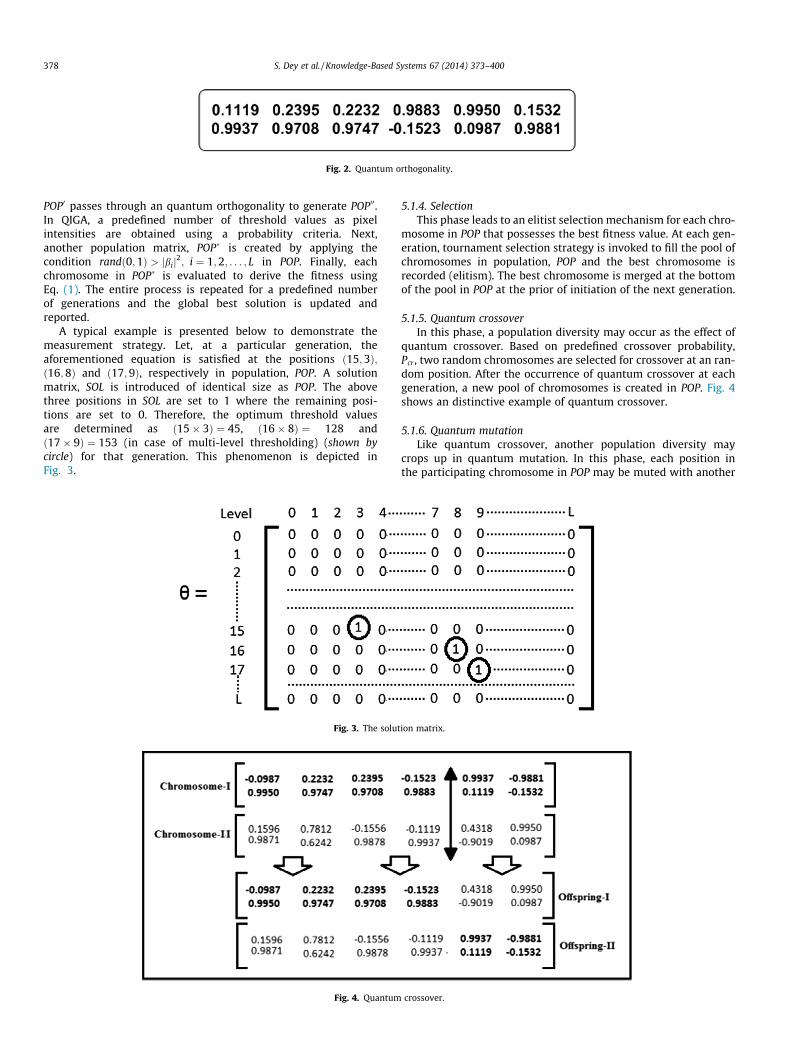
Fig. 2. Quantum orthogonality.


POP0 passes through an quantum orthogonality to generate POP00.In QIGA, a predefined number of threshold values as pixelintensities are obtained using a probability criteria. Next,another population matrix, POP� is created by applying thecondition randð0;1Þ > jbij

2; i ¼ 1;2; . . . ; L in POP. Finally, each

chromosome in POP� is evaluated to derive the fitness usingEq. (1). The entire process is repeated for a predefined numberof generations and the global best solution is updated andreported.

A typical example is presented below to demonstrate themeasurement strategy. Let, at a particular generation, theaforementioned equation is satisfied at the positions ð15;3Þ;ð16;8Þ and ð17;9Þ, respectively in population, POP. A solutionmatrix, SOL is introduced of identical size as POP. The abovethree positions in SOL are set to 1 where the remaining posi-tions are set to 0. Therefore, the optimum threshold valuesare determined as ð15� 3Þ ¼ 45, ð16� 8Þ ¼ 128 andð17� 9Þ ¼ 153 (in case of multi-level thresholding) (shown bycircle) for that generation. This phenomenon is depicted inFig. 3.

Fig. 4. Quantum

Fig. 3. The solut

5.1.4. SelectionThis phase leads to an elitist selection mechanism for each chro-

mosome in POP that possesses the best fitness value. At each gen-eration, tournament selection strategy is invoked to fill the pool ofchromosomes in population, POP and the best chromosome isrecorded (elitism). The best chromosome is merged at the bottomof the pool in POP at the prior of initiation of the next generation.

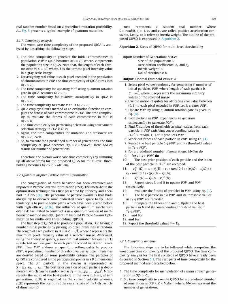
5.1.5. Quantum crossoverIn this phase, a population diversity may occur as the effect of

quantum crossover. Based on predefined crossover probability,Pcr , two random chromosomes are selected for crossover at an ran-dom position. After the occurrence of quantum crossover at eachgeneration, a new pool of chromosomes is created in POP. Fig. 4shows an distinctive example of quantum crossover.

5.1.6. Quantum mutationLike quantum crossover, another population diversity may

crops up in quantum mutation. In this phase, each position inthe participating chromosome in POP may be muted with another

crossover.

ion matrix.


real random number based on a predefined mutation probability,Pm. Fig. 5 presents a typical example of quantum mutation.

5.1.7. Complexity analysisThe worst case time complexity of the proposed QIGA is ana-

lyzed by describing the following steps.

1. The time complexity to generate the initial chromosomes inpopulation, POP in QIGA becomes OðV � LÞ, where, V representsthe population size in QIGA. Note that, the length of each chro-mosome is L ¼

ffiffiffiLp

where, L is the utmost pixel intensity valuein a gray scale image.

2. For assigning real value to each pixel encoded in the populationof chromosomes in POP, the time complexity of QIGA turns intoOðV � LÞ.

3. The time complexity for updating POP0 using quantum rotationgate in QIGA becomes OðV � LÞ.

4. The time complexity for quantum orthogonality in QIGA isOðV � LÞ.

5. The time complexity to create POP� is OðV � LÞ.6. QIGA employs Otsu’s method as an evaluation function to com-

pute the fitness of each chromosome in POP. The time complex-ity to evaluate the fitness of each chromosome in POP isOðV � KÞ.

7. The time complexity for performing selection using tournamentselection strategy in POP is OðVÞ.

8. Again, the time complexities for mutation and crossover areOðV � LÞ each.

9. So, to execute for a predefined number of generations, the timecomplexity of QIGA becomes OðV � L �MxGenÞ. Here, MxGenstands for number of generations.

Therefore, the overall worst case time complexity (by summingup all above steps) for the proposed QIGA for multi-level thres-holding becomes OðV � L �MxGenÞ.

5.2. Quantum Inspired Particle Swarm Optimization

The congregation of bird’s behavior has been examined andimposed in Particle Swarm Optimization (PSO). This meta-heuristicoptimization technique was first presented by Kennedy and Eber-hart in 1995 [36]. The panorama of particle swarm is that birdsalways try to discover some dedicated search space to fly. Theirtendency is to pursue some paths which have been visited beforewith high efficacy [2,36]. The influence of quantum mechanismover PSO facilitated to construct a new quantum version of meta-heuristic method namely, Quantum Inspired Particle Swarm Opti-mization for multi-level thresholding (QIPSO).

The first step of QIPSO is to produce a population, POP having Vnumber initial particles by picking up pixel intensities at random.The length of each particle in POP is L ¼

ffiffiffiLp

, where L represents themaximum pixel intensity value of a selected image. Afterward,using the theory of qubits, a random real number between (0,1)is selected and assigned to each pixel encoded in POP to createPOP0. Then POP0 endures an quantum orthogonality to producePOP00. A predefined number of threshold values as pixel intensitiesare derived based on some probability criteria. The particles ofQIPSO are considered as the participating points in a D dimensionalspace. The jth particle in the swarm is represented asS ¼ ðsj1; sj2; . . . ; sjDÞ. The best prior position of each particle is docu-mented, which can be symbolized as Pk ¼ ðpk1; pk2; . . . ; pkDÞ

T . b rep-resents the index of the best particle in the swarm. Here, at t-thgeneration, v t

kðDÞ is regarded as the current velocity whereas,st

kðDÞ represents the position at the search space of the k-th particleof dimension D.

rand represents a random real number where0 6 randð0;1Þ 6 1. c1 and c2 are called positive acceleration con-stants. Lastly, x is refers to inertia weight. The outline of the pro-posed QIPSO is expressed in Algorithm 2.

Algorithm 2. Steps of QIPSO for multi-level thresholding

Input: Number of Generation: MxGenSize of the population: VAcceleration coefficients: c1 and c2

Inertia weight: xNo. of thresholds: K


1: Select pixel values randomly for generating V number ofinitial particles, POP, where length of each particle isL ¼

ffiffiffiLp

, where, L represents the maximum intensityvalues of the selected image.

2: Use the notion of qubits for allocating real value between(0,1) to each pixel encoded in POP. Let it creates POP0.

3: Update POP0 by using quantum rotation gate as given inEq. (4).

4: Each particle in POP0 experiences an quantumorthogonality to generate POP00.

5: Find K number of thresholds as pixel values from eachparticle in POP satisfying corresponding value inPOP00 > randð0;1Þ. Let it produces POP�.

6: Work out fitness of each particle in POP� using Eq. (1).7: Record the best particle b 2 POP00 and its threshold values

in TB 2 POP�.8: for a predefined number of generations, MxGen do9: for all k 2 POP00 do

10: The best prior position of each particle and the indexof the best particle in POP00 are recorded.

11: v tþ1k ðDÞ ¼ x � v t

kðDÞ þ c1 � randð0;1Þ � ðptkðDÞ � st

kðDÞÞþc2 � randð0;1Þ � ðpt

uðDÞ � stkðDÞÞ.

12: stþ1k ðDÞ ¼ st

kðDÞ þ v tþ1k ðDÞ.

13: Repeat steps 3 and 5 to update POP0 and POP�

respectively.14: Evaluate the fitness of particles in POP� using Eq. (1).15: The best particle in c 2 POP0 and its threshold values

in TB 2 POP� are recorded.16: Compare the fitness of b and c. Update the best

particle in b and its corresponding threshold values inTB 2 POP�.

17: end for18: end for19: Report the threshold values h ¼ TB.

5.2.1. Complexity analysis

The following steps are to be followed while computing theworst case time complexity of the proposed QIPSO. The time com-plexity analysis for the first six steps of QIPSO have already beendiscussed in Section 5.1. The rest parts of time complexity for theproposed method are described below.

1. The time complexity for manipulation of swarm at each gener-ation is OðV � LÞ.

2. So, time complexity to execute QIPSO for a predefined numberof generations is OðV � L �MxGenÞ where, MxGen represent thenumber of generations.

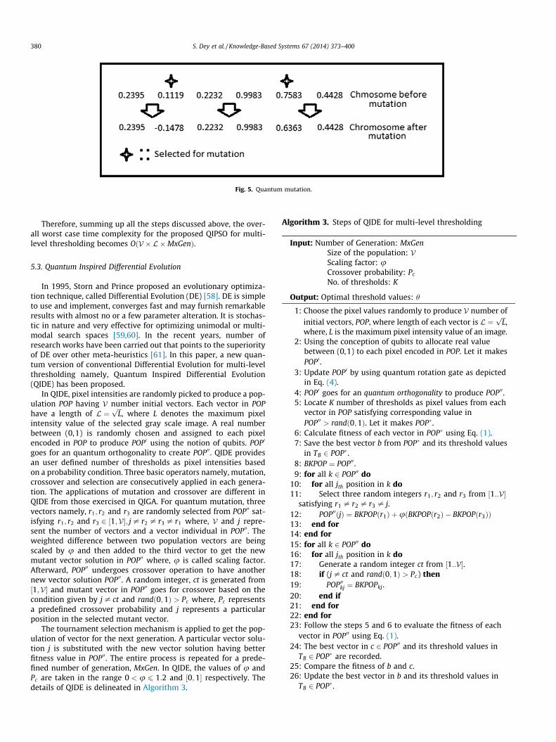
Fig. 5. Quantum mutation.


Therefore, summing up all the steps discussed above, the over-all worst case time complexity for the proposed QIPSO for multi-level thresholding becomes OðV � L �MxGenÞ.

5.3. Quantum Inspired Differential Evolution

In 1995, Storn and Prince proposed an evolutionary optimiza-tion technique, called Differential Evolution (DE) [58]. DE is simpleto use and implement, converges fast and may furnish remarkableresults with almost no or a few parameter alteration. It is stochas-tic in nature and very effective for optimizing unimodal or multi-modal search spaces [59,60]. In the recent years, number ofresearch works have been carried out that points to the superiorityof DE over other meta-heuristics [61]. In this paper, a new quan-tum version of conventional Differential Evolution for multi-levelthresholding namely, Quantum Inspired Differential Evolution(QIDE) has been proposed.

In QIDE, pixel intensities are randomly picked to produce a pop-ulation POP having V number initial vectors. Each vector in POPhave a length of L ¼

ffiffiffiLp

, where L denotes the maximum pixelintensity value of the selected gray scale image. A real numberbetween (0,1) is randomly chosen and assigned to each pixelencoded in POP to produce POP0 using the notion of qubits. POP0

goes for an quantum orthogonality to create POP00. QIDE providesan user defined number of thresholds as pixel intensities basedon a probability condition. Three basic operators namely, mutation,crossover and selection are consecutively applied in each genera-tion. The applications of mutation and crossover are different inQIDE from those exercised in QIGA. For quantum mutation, threevectors namely, r1; r2 and r3 are randomly selected from POP00 sat-isfying r1; r2 and r3 2 ½1;V�; j – r2 – r3 – r1 where, V and j repre-sent the number of vectors and a vector individual in POP00. Theweighted difference between two population vectors are beingscaled by u and then added to the third vector to get the newmutant vector solution in POP00 where, u is called scaling factor.Afterward, POP00 undergoes crossover operation to have anothernew vector solution POP00. A random integer, ct is generated from½1;V� and mutant vector in POP00 goes for crossover based on thecondition given by j – ct and randð0;1Þ > Pc where, Pc representsa predefined crossover probability and j represents a particularposition in the selected mutant vector.

The tournament selection mechanism is applied to get the pop-ulation of vector for the next generation. A particular vector solu-tion j is substituted with the new vector solution having betterfitness value in POP00. The entire process is repeated for a prede-fined number of generation, MxGen. In QIDE, the values of u andPc are taken in the range 0 < u 6 1:2 and ½0;1� respectively. Thedetails of QIDE is delineated in Algorithm 3.

Algorithm 3. Steps of QIDE for multi-level thresholding

Input: Number of Generation: MxGenSize of the population: VScaling factor: uCrossover probability: Pc

No. of thresholds: K


1: Choose the pixel values randomly to produce V number ofinitial vectors, POP, where length of each vector is L ¼

ffiffiffiLp

,where, L is the maximum pixel intensity value of an image.

2: Using the conception of qubits to allocate real valuebetween (0,1) to each pixel encoded in POP. Let it makesPOP0.

3: Update POP0 by using quantum rotation gate as depictedin Eq. (4).

4: POP0 goes for an quantum orthogonality to produce POP00.5: Locate K number of thresholds as pixel values from each

vector in POP satisfying corresponding value inPOP00 > randð0;1Þ. Let it makes POP�.

6: Calculate fitness of each vector in POP� using Eq. (1).7: Save the best vector b from POP� and its threshold values

in TB 2 POP�.8: BKPOP ¼ POP00.9: for all k 2 POP00 do

10: for all jth position in k do11: Select three random integers r1; r2 and r3 from ½1::V�

satisfying r1 – r2 – r3 – j.12: POP00ðjÞ ¼ BKPOPðr1Þ þuðBKPOPðr2Þ � BKPOPðr3ÞÞ13: end for14: end for15: for all k 2 POP00 do16: for all jth position in k do17: Generate a random integer ct from ½1::V�.18: if (j – ct and randð0;1Þ > Pc) then19: POP00kj ¼ BKPOPkj.20: end if21: end for22: end for23: Follow the steps 5 and 6 to evaluate the fitness of each

vector in POP00 using Eq. (1).24: The best vector in c 2 POP00 and its threshold values in

TB 2 POP� are recorded.25: Compare the fitness of b and c.26: Update the best vector in b and its threshold values in

TB 2 POP�.


27: for all k 2 POP00 do28: if (Fitness of BKPOPk is better than the fitness of POP00k)

then29: POP00ðkÞ ¼ BKPOPk.30: end if31: end for32: POP00 undergoes an quantum orthogonality.33: Repeat steps 5 to 31 for fixed number of generation,

MxGen.34: The optimal threshold values, h ¼ TB are reported.

5.3.1. Complexity analysis

The outline of worst case time complexity analysis of the pro-posed QIDE is described below. The first six steps of time complex-ity analysis for QIDE have already been illustrated in Section 5.1.The worst case time complexity analysis for the next parts of QIDEare given below.

1. Time complexities for mutation, crossover and the selectionparts entail OðV � LÞ.

2. So, to execute QIDE for a predefined number of generations, thetime complexity becomes OðV � L �MxGenÞ. Here, MxGen sig-nifies the number of generations.

Therefore, aggregating the overall discussion as stated above, itcan be concluded that the worst case time complexity for the pro-posed QIDE for multi-level thresholding is OðV � L �MxGenÞ.

5.4. Quantum Inspired Ant Colony Optimization

In 1996, Dorigo et al. presented a population-based optimiza-tion technique, called Ant Colony Optimization (ACO) [62]. ACOimitates the basic behaviors of real ants to accomplish the solu-tions of various optimization problem. In real life, ants strugglefor food to sustain their existence. They traverse different pathsfor food and squirt a chemical called pheromone from their body.This chemical helps them to exchange information among them-selves and to locate the shortest path to be followed between theirnest and a food source. It is be observed that a particular pathwhich contains more amount of pheromone, is outlined by morenumber of ants. Many scholars have been motivated by the com-munal behavior of real ants and established numerous algorithmsfor solving combinatorial optimization problems [42].

In the proposed Quantum Inspired Ant Colony Optimization(QIACO), pixel intensities are randomly selected to create a popu-lation POP having V number initial strings. The length of eachstring in POP is L ¼

ffiffiffiLp

, where L is the utmost pixel intensity valuein a gray scale image. Using the concept of qubits, a real randomnumber between (0,1) is generated and allocated to each pixelencoded in POP to create POP0. Then POP0 undergoes an quantumorthogonality to produce POP00. Based on a probability condition,the method resorts to an user defined number of thresholds aspixel intensity values. At each generation, the method exploresthe best search path. At the outset, a pheromone matrix, sj is gen-erated for each ant, j. For each individual j 2 POP00, the maximumpheromone integration is deduced as threshold value in the grayscale image, if POP00ðjÞ > q0. Here, q0 is the priory defined numberwhere, 0 6 q0 6 1. This leads to POP00ðkjÞ ¼ arg maxskj. IfPOP00ðjÞ 6 q0; POP00ðkjÞ ¼ randð0;1Þ. The pheromone trial matrix isupdated at the end of each generation using skj ¼ qskj þ ð1� qÞbwhere, b represents the best string of each generation and k repre-sents the corresponding position in a particular string, j. In QIACO,MxGen represents the number of generations to be executed,K and V are the user defined number of thresholds and population

size, respectively. q is known as persistence of trials, q 2 ½0;1�. Thedetails of the proposed QIACO is illustrated in Algorithm 4.

5.4.1. Complexity analysisThe worst case time complexity of the proposed QIACO is ana-

lyzed in this section. The time complexities of the first six steps ofQIGA and QIACO are identical, which are already discussed in theSection 5.1. The time complexity analysis for the remaining partsof proposed QIACO are given below.

1. The time complexity to construct the pheromone matrix, s isOðV � LÞ.

2. The time complexity to determine POP�� from s at each gener-ation is OðV � LÞ.

3. The pheromone matrix is needed to be updated at each gener-ation. The time complexity for this computation is OðLÞ

4. Again, time complexity to execute for a predefined number ofgenerations for QIACO is OðV � L �MxGenÞ, where, MxGen isthe number of generations.

Algorithm 4. Steps of QIACO for multi-level thresholding

Input: Number of Generation: MxGenSize of the population: VNo. of thresholds: KPersistence of trials: qPriory defined number: q0


1: The pixel values are randomly selected to generate Vnumber of initial strings, POP, where length of each stringis L ¼

ffiffiffiLp

, where, L signifies the greatest pixel value of thegray scale image.

2: The thought of qubits is employed to assign real value between(0,1) to each pixel encoded in POP. Let it produces POP0.

3: Quantum rotation gate is employed to update POP0 usingEq. (4).

4: POP0 endures an quantum orthogonality to create POP00.5: Finding K number of thresholds as pixel values from each

string in POP satisfying corresponding value inPOP00 > randð0;1Þ. Let it creates POP�.

6: Evaluate fitness of each string in POP� using Eq. (1).7: Save the best string b from POP�.8: Repeat step (5) to produce POP��.9: Construct the pheromone matrix, s.

10: for a fixed number of generations (MxGen) do11: for all j 2 POP00 do12: for all kth location in j do13: if (randð0;1Þ > q0) then14: POP00jk ¼ arg maxsjk.15: else16: POP00jk ¼ randð0;1Þ.17: end if18: end for19: end for20: Use Eq. (1) to calculate the fitness of POP00.21: Save the best string c from POP��.22: The fitness of b and c is compared.23: Use POP�� to update the string with best string along of

its corresponding threshold values in TBS.24: Save the best string of step (22) in b and its

corresponding thresholds TBS 2 POP��.25: for all j 2 POP00 do

(continued on next page)


26: for all kth location in j do27: sjk ¼ qsjk þ ð1� qÞb.28: end for29: end for30: end for31: Report the threshold values h ¼ TBS.

Therefore, summing up all the steps discussed above, the over-all worst case time complexity for the proposed QIACO for multi-level thresholding becomes OðV � L �MxGenÞ.

5.5. Quantum Inspired Simulated Annealing

In 1983, Kirkpatrick et al. first used Simulated annealing (SA) asa search algorithm for optimization [63]. The basic principle of thismeta-heuristic optimization technique is to heat a physical bodywith a very high temperature and then cool it gradually to forma sturdy chemical structure. This chemical phenomena is calledcrystallization. A strategy is introduced in SA that ensures avoidingto stuck at its local minima. In this subsection, a variant QuantumInspired Simulated Annealing for multi-level thresholding (QISA) ispresented.

Initially, an initial configuration, P is created by choosing thepixel intensities randomly of length L ¼

ffiffiffiLp

, where, L representsthe highest pixel intensity value in a gray scale image. The theoryof qubits is employed to a newly introduced encoded scheme toallocate real random value between (0,1) to each pixel encodedin P and it is named as P0. Afterward, P0 goes for an quantumorthogonality to create P00. QISA finds an user defined numberof thresholds as pixel intensities based on a defined probabilitycondition. Firstly, a very high temperature, T max is assigned to anewly invoked temperature parameter, T . QISA is allowed to exe-cute for I number of iterations for each temperature. Thereafter,T is reduced by a reduction factor, t. The execution continuesuntil T reaches at the predefined final temperature, T min. At eachiteration of I , a better configuration, ðSÞ may expected becausethe old configuration is perturbed randomly at multiple points.Subsequently, a new configuration, S� is generated from S byenduring the similar process which was acclimatized before tocreate P� from P. The acceptance of the configurations S and S�

depends on the condition given by FðS�Þ > FðP�Þ, by revisingthe previous configurations P and P�, respectively; otherwise,the newly generated configuration may be admitted with a prob-ability expð�ðFðP�Þ � FðS�ÞÞÞ=T . In general, the probability isdetermined by the Boltzmann distribution. t is chosen withinthe range of ½0:5;0:99� whereas, K signifies user defined numberof thresholds. h represents the output as thresholds. The detailsof the proposed QIGA for multi-level thresholding is describedin Algorithm 5.

5.5.1. Complexity analysisThe following steps describes the worst case time complexity

for the proposed QISA for multi-level thresholding.

1. For initial configuration in QISA, the time complexity is OðLÞ,where length of configuration is L ¼

ffiffiffiLp

where, L signifies themaximum intensity value of a gray scale image.

2. For assignment of real value to each pixel encoded in the pop-ulation of configuration, the time complexity is OðLÞ.

3. The time complexity for updating P0 turns into OðLÞ.4. The time complexity to perform quantum orthogonality is OðLÞ.5. The time complexity to create P� is OðLÞ.6. The time complexity for fitness computation using Eq. (1) turns

into OðKÞ.

7. In a similar way, for the fitness computation of the configura-tion after perturbation, the time complexity is OðKÞ.

8. Let the outer loop and inner loop are executed MxIn and I timesrespectively in QISA. Therefore, the time complexity to executethis step in QISA happens to be I �MxIn.

Algorithm 5. Steps of QISA for multi-level thresholding

Input: Initial temperature: T max

Final temperature: T min

Reduction factor: tNo. of thresholds: KNumber of Iterations: I


1: Randomly select pixel intensities to create an initialconfiguration, P, where length of the configuration isdenoted by L ¼

ffiffiffiLp

, where, L is taken as the maximumintensity value of a gray scale image.

2: Apply the thought of qubits to assign real value between(0,1) to each pixel encoded in P. Let it generates P0.

3: Quantum rotation gate is used to update P0 using Eq. (4).4: The configuration in P0 passes through an quantum

orthogonality to generate P00.5: Discover K number of thresholds as pixel intensities from

the configuration in P. It should hold corresponding valuein P00 > randð0;1Þ. Let it generates P�.

6: Evaluate fitness of the configuration in P� using Eq. (1). Letit be symbolized by FðP�Þ.

7: T ¼ T max.8: repeat9: for j ¼ 1 to I do

10: Perturb P. Let it create S.11: Repeat step (2), (3) and (4) to create S�.12: Use Eq. (1) to evaluate fitness EðS�; TÞ of the

configuration S�.13: if (FðS�Þ � FðP�Þ > 0) then14: Set P ¼ S; P� ¼ S� and FðP�Þ ¼ FðS�Þ.15: else16: Set P ¼ S; P� ¼ S� and FðP�Þ ¼ FðS�Þ with

probability expð�ðFðP�Þ � FðS�ÞÞÞ=T .17: end if18: end for19: T ¼ T � t.20: until T >¼ T min

21: Report the optimal threshold values, h ¼ P�.

Therefore, aggregating the steps discussed above, the proposedQISA for multi-level thresholding possesses the worst case timecomplexity OðL � I �MxInÞ.

5.6. Quantum Inspired Tabu Search

The Tabu Search (TS) is a popular meta-heuristic technique thatwas first proposed by Glover and Laguna in 1997 [52]. The search-ing mechanism facilitates TS to trounce local optima. So, it explorethe solution space to let it go for hill climbing. It incorporates theconcept of adaptive memory strategy, popularly known as tabumemory to record the intermediate tabu restrictions. Basically, thiskind of memory stores the information regarding solution attri-butes that may require while transforming from one solution moveto another. The functionality of TS may be described as the

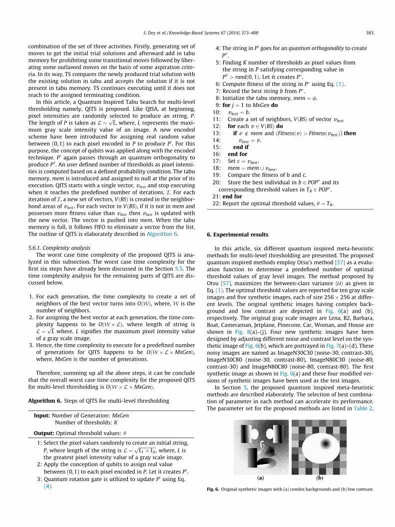
Fig. 6. Original synthetic images with (a) comlex backgrounds and (b) low contrast.


combination of the set of three activities. Firstly, generating set ofmoves to get the initial trial solutions and afterward add in tabumemory for prohibiting some transitional moves followed by liber-ating some outlawed moves on the basis of some aspiration crite-ria. In its way, TS compares the newly produced trial solution withthe existing solution in tabu and accepts the solution if it is notpresent in tabu memory. TS continues executing until it does notreach to the assigned terminating condition.

In this article, a Quantum Inspired Tabu Search for multi-levelthresholding namely, QITS is proposed. Like QISA, at beginning,pixel intensities are randomly selected to produce an string, P.The length of P is taken as L ¼

ffiffiffiLp

, where, L represents the maxi-mum gray scale intensity value of an image. A new encodedscheme have been introduced for assigning real random valuebetween (0,1) to each pixel encoded in P to produce P0. For thispurpose, the concept of qubits was applied along with the encodedtechnique. P0 again passes through an quantum orthogonality toproduce P00. An user defined number of thresholds as pixel intensi-ties is computed based on a defined probability condition. The tabumemory, mem is introduced and assigned to null at the prior of itsexecution. QITS starts with a single vector, vbest and stop executingwhen it reaches the predefined number of iterations, I . For eachiteration of I , a new set of vectors, VðBSÞ is created in the neighbor-hood areas of vbest . For each vector in VðBSÞ, if it is not in mem andpossesses more fitness value than vbest then vbest is updated withthe new vector. The vector is pushed into mem. When the tabumemory is full, it follows FIFO to eliminate a vector from the list.The outline of QITS is elaborately described in Algorithm 6.

5.6.1. Complexity analysisThe worst case time complexity of the proposed QITS is ana-

lyzed in this subsection. The worst case time complexity for thefirst six steps have already been discussed in the Section 5.5. Thetime complexity analysis for the remaining parts of QITS are dis-cussed below.

1. For each generation, the time complexity to create a set ofneighbors of the best vector turns into OðWÞ, where, W is thenumber of neighbors.

2. For assigning the best vector at each generation, the time com-plexity happens to be OðW � LÞ, where length of string isL ¼

ffiffiffiLp

where, L signifies the maximum pixel intensity valueof a gray scale image.

3. Hence, the time complexity to execute for a predefined numberof generations for QITS happens to be OðW � L�MxGenÞ,where, MxGen is the number of generations.

Therefore, summing up all the above steps, it can be concludethat the overall worst case time complexity for the proposed QITSfor multi-level thresholding is OðW � L �MxGenÞ.

Algorithm 6. Steps of QITS for multi-level thresholding

Input: Number of Generation: MxGenNumber of thresholds: K


1: Select the pixel values randomly to create an initial string,P, where length of the string is L ¼

ffiffiffiffiffiffiffiffiffiffiffiffiffiffiffiL1 � L2p

, where, L isthe greatest pixel intensity value of a gray scale image.

2: Apply the conception of qubits to assign real valuebetween (0,1) to each pixel encoded in P. Let it creates P0.

3: Quantum rotation gate is utilized to update P0 using Eq.(4).

4: The string in P0 goes for an quantum orthogonality to createP00.

5: Finding K number of thresholds as pixel values fromthe string in P satisfying corresponding value inP00 > randð0;1Þ. Let it creates P�.

6: Compute fitness of the string in P� using Eq. (1).7: Record the best string b from P�.8: Initialize the tabu memory, mem ¼ /.9: for j ¼ 1 to MxGen do

10: vbest ¼ b.11: Create a set of neighbors, VðBSÞ of vector vbest

12: for each v 2 VðBSÞ do13: if v R mem and ðFitnessðvÞ > FitnessðvbestÞ) then14: vbest ¼ v .15: end if16: end for17: Set c ¼ vbest .18: mem ¼ mem [ vbest .19: Compare the fitness of b and c.20: Store the best individual in b 2 POP00 and its

corresponding threshold values in TB 2 POP�.21: end for22: Report the optimal threshold values, h ¼ TB.

6. Experimental results

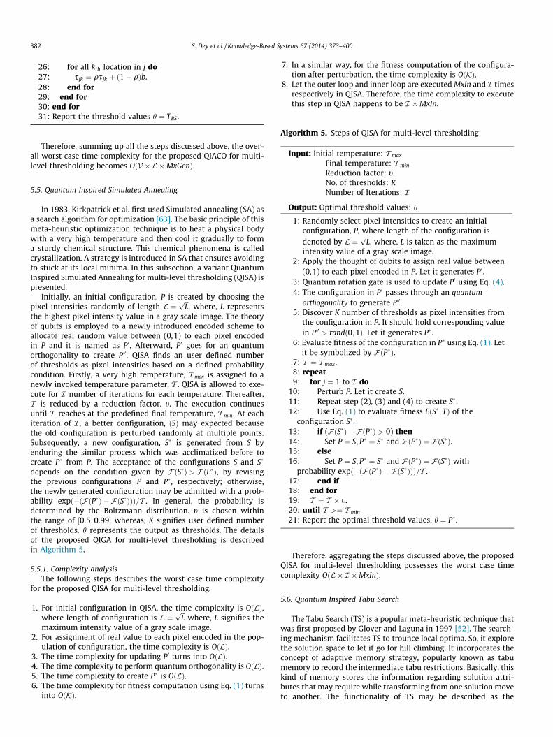
In this article, six different quantum inspired meta-heuristicmethods for multi-level thresholding are presented. The proposedquantum inspired methods employ Otsu’s method [57] as a evalu-ation function to determine a predefined number of optimalthreshold values of gray level images. The method proposed byOtsu [57], maximizes the between-class variance ðUÞ as given inEq. (1). The optimal threshold values are reported for ten gray scaleimages and five synthetic images, each of size 256� 256 at differ-ent levels. The original synthetic images having complex back-ground and low contrast are depicted in Fig. 6(a) and (b),respectively. The original gray scale images are Lena, B2, Barbara,Boat, Cameraman, Jetplane, Pinecone, Car, Woman, and House areshown in Fig. 8(a)–(j). Four new synthetic images have beendesigned by adjusting different noise and contrast level on the syn-thetic image of Fig. 6(b), which are portrayed in Fig. 7(a)–(d). Thesenoisy images are named as ImageN30C30 (noise-30, contrast-30),ImageN30C80 (noise-30, contrast-80), ImageN80C30 (noise-80,contrast-30) and ImageN80C80 (noise-80, contrast-80). The firstsynthetic image as shown in Fig. 6(a) and these four modified ver-sions of synthetic images have been used as the test images.

In Section 5, the proposed quantum inspired meta-heuristicmethods are described elaborately. The selection of best combina-tion of parameter in each method can accelerate its performance.The parameter set for the proposed methods are listed in Table 2.

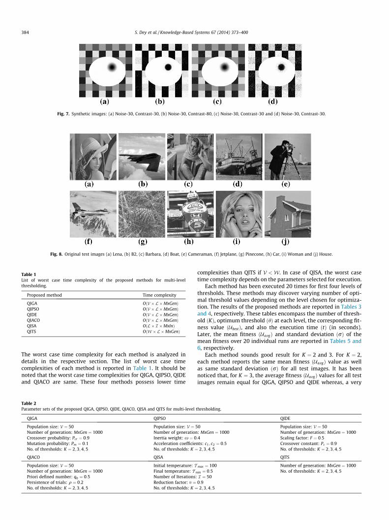
Fig. 8. Original test images (a) Lena, (b) B2, (c) Barbara, (d) Boat, (e) Cameraman, (f) Jetplane, (g) Pinecone, (h) Car, (i) Woman and (j) House.

Fig. 7. Synthetic images: (a) Noise-30, Contrast-30, (b) Noise-30, Contrast-80, (c) Noise-30, Contrast-30 and (d) Noise-30, Contrast-30.

Table 1List of worst case time complexity of the proposed methods for multi-levelthresholding.

Proposed method Time complexity

QIGA OðV � L �MxGenÞQIPSO OðV � L �MxGenÞQIDE OðV � L �MxGenÞQIACO OðV � L �MxGenÞQISA OðL � I �MxInÞQITS OðW � L �MxGenÞ


The worst case time complexity for each method is analyzed indetails in the respective section. The list of worst case timecomplexities of each method is reported in Table 1. It should benoted that the worst case time complexities for QIGA, QIPSO, QIDEand QIACO are same. These four methods possess lower time

Table 2Parameter sets of the proposed QIGA, QIPSO, QIDE, QIACO, QISA and QITS for multi-level

QIGA QIPSO

Population size: V ¼ 50 Population size: V ¼ 5Number of generation: MxGen ¼ 1000 Number of generationCrossover probability: Pcr ¼ 0:9 Inertia weight: x ¼ 0Mutation probability: Pm ¼ 0:1 Acceleration coefficieNo. of thresholds: K ¼ 2;3;4;5 No. of thresholds: K ¼

QIACO QISA

Population size: V ¼ 50 Initial temperature: TNumber of generation: MxGen ¼ 1000 Final temperature: TPriori defined number: q0 ¼ 0:5 Number of Iterations:Persistence of trials: q ¼ 0:2 Reduction factor: t ¼No. of thresholds: K ¼ 2;3;4;5 No. of thresholds: K ¼

complexities than QITS if V <W. In case of QISA, the worst casetime complexity depends on the parameters selected for execution.

Each method has been executed 20 times for first four levels ofthresholds. These methods may discover varying number of opti-mal threshold values depending on the level chosen for optimiza-tion. The results of the proposed methods are reported in Tables 3and 4, respectively. These tables encompass the number of thresh-old ðKÞ, optimum threshold ðhÞ at each level, the corresponding fit-ness value ðUbestÞ, and also the execution time ðtÞ (in seconds).Later, the mean fitness ðUavgÞ and standard deviation ðrÞ of themean fitness over 20 individual runs are reported in Tables 5 and6, respectively.

Each method sounds good result for K ¼ 2 and 3. For K ¼ 2,each method reports the same mean fitness ðUavgÞ value as wellas same standard deviation ðrÞ for all test images. It has beennoticed that, for K ¼ 3, the average fitness ðUavgÞ values for all testimages remain equal for QIGA, QIPSO and QIDE whereas, a very

thresholding.

QIDE

0 Population size: V ¼ 50: MxGen ¼ 1000 Number of generation: MxGen ¼ 1000:4 Scaling factor: F ¼ 0:5nts: c1; c2 ¼ 0:5 Crossover constant: Pc ¼ 0:9

2;3;4;5 No. of thresholds: K ¼ 2;3;4;5

QITS

max ¼ 100 Number of generation: MxGen ¼ 1000

min ¼ 0:5 No. of thresholds: K ¼ 2;3;4;5I ¼ 500:92;3;4;5

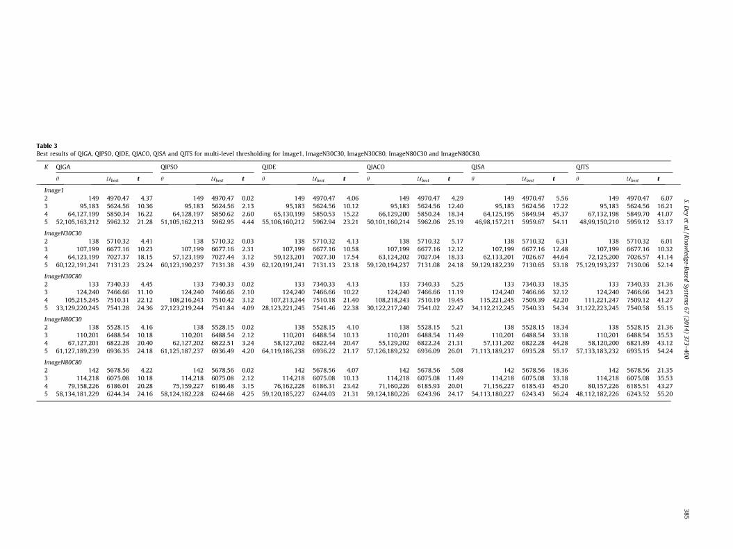
Table 3Best results of QIGA, QIPSO, QIDE, QIACO, QISA and QITS for multi-level thresholding for Image1, ImageN30C30, ImageN30C80, ImageN80C30 and ImageN80C80.

K QIGA QIPSO QIDE QIACO QISA QITS

h Ubest t h Ubest t h Ubest t h Ubest t h Ubest t h Ubest t

Image12 149 4970.47 4.37 149 4970.47 0.02 149 4970.47 4.06 149 4970.47 4.29 149 4970.47 5.56 149 4970.47 6.073 95,183 5624.56 10.36 95,183 5624.56 2.13 95,183 5624.56 10.12 95,183 5624.56 12.40 95,183 5624.56 17.22 95,183 5624.56 16.214 64,127,199 5850.34 16.22 64,128,197 5850.62 2.60 65,130,199 5850.53 15.22 66,129,200 5850.24 18.34 64,125,195 5849.94 45.37 67,132,198 5849.70 41.075 52,105,163,212 5962.32 21.28 51,105,162,213 5962.95 4.44 55,106,160,212 5962.94 23.21 50,101,160,214 5962.06 25.19 46,98,157,211 5959.67 54.11 48,99,150,210 5959.12 53.17

ImageN30C302 138 5710.32 4.41 138 5710.32 0.03 138 5710.32 4.13 138 5710.32 5.17 138 5710.32 6.31 138 5710.32 6.013 107,199 6677.16 10.23 107,199 6677.16 2.31 107,199 6677.16 10.58 107,199 6677.16 12.12 107,199 6677.16 12.48 107,199 6677.16 10.324 64,123,199 7027.37 18.15 57,123,199 7027.44 3.12 59,123,201 7027.30 17.54 63,124,202 7027.04 18.33 62,133,201 7026.67 44.64 72,125,200 7026.57 41.145 60,122,191,241 7131.23 23.24 60,123,190,237 7131.38 4.39 62,120,191,241 7131.13 23.18 59,120,194,237 7131.08 24.18 59,129,182,239 7130.65 53.18 75,129,193,237 7130.06 52.14

ImageN30C802 133 7340.33 4.45 133 7340.33 0.02 133 7340.33 4.13 133 7340.33 5.25 133 7340.33 18.35 133 7340.33 21.363 124,240 7466.66 11.10 124,240 7466.66 2.10 124,240 7466.66 10.22 124,240 7466.66 11.19 124,240 7466.66 32.12 124,240 7466.66 34.234 105,215,245 7510.31 22.12 108,216,243 7510.42 3.12 107,213,244 7510.18 21.40 108,218,243 7510.19 19.45 115,221,245 7509.39 42.20 111,221,247 7509.12 41.275 33,129,220,245 7541.28 24.36 27,123,219,244 7541.84 4.09 28,123,221,245 7541.46 22.38 30,122,217,240 7541.02 22.47 34,112,212,245 7540.33 54.34 31,122,223,245 7540.58 55.15

ImageN80C302 138 5528.15 4.16 138 5528.15 0.02 138 5528.15 4.10 138 5528.15 5.21 138 5528.15 18.34 138 5528.15 21.363 110,201 6488.54 10.18 110,201 6488.54 2.12 110,201 6488.54 10.13 110,201 6488.54 11.49 110,201 6488.54 33.18 110,201 6488.54 35.534 67,127,201 6822.28 20.40 62,127,202 6822.51 3.24 58,127,202 6822.44 20.47 55,129,202 6822.24 21.31 57,131,202 6822.28 44.28 58,120,200 6821.89 43.125 61,127,189,239 6936.35 24.18 61,125,187,237 6936.49 4.20 64,119,186,238 6936.22 21.17 57,126,189,232 6936.09 26.01 71,113,189,237 6935.28 55.17 57,133,183,232 6935.15 54.24

ImageN80C802 142 5678.56 4.22 142 5678.56 0.02 142 5678.56 4.07 142 5678.56 5.08 142 5678.56 18.36 142 5678.56 21.353 114,218 6075.08 10.18 114,218 6075.08 2.12 114,218 6075.08 10.13 114,218 6075.08 11.49 114,218 6075.08 33.18 114,218 6075.08 35.534 79,158,226 6186.01 20.28 75,159,227 6186.48 3.15 76,162,228 6186.31 23.42 71,160,226 6185.93 20.01 71,156,227 6185.43 45.20 80,157,226 6185.51 43.275 58,134,181,229 6244.34 24.16 58,124,182,228 6244.68 4.25 59,120,185,227 6244.03 21.31 59,124,180,226 6243.96 24.17 54,113,180,227 6243.43 56.24 48,112,182,226 6243.52 55.20

S.Dey

etal./K

nowledge-Based

Systems

67(2014)

373–400

385

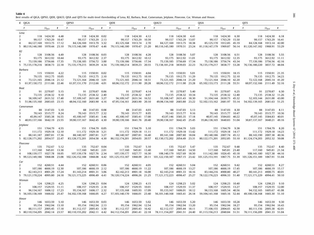
Table 4Best results of QIGA, QIPSO, QIDE, QIACO, QISA and QITS for multi-level thresholding of Lena, B2, Barbara, Boat, Cameraman, Jetplane, Pinecone, Car, Woman and House.



Lena2 118 1424.30 4.48 118 1424.30 0.02 118 1424.30 4.12 118 1424.30 4.41 118 1424.30 6.30 118 1424.30 6.183 99,157 1763.29 10.47 99,157 1763.29 2.13 99,157 1763.29 10.39 99,157 1763.29 13.07 99,157 1763.29 15.50 99,157 1763.29 16.414 84,127,169 1913.75 17.12 84,126,169 1913.79 3.32 83,125,168 1913.74 2.70 84,127,169 1913.75 18.38 85,125,170 1912.85 45.19 84,128,168 1913.14 42.005 80,116,146,180 1970.44 23.10 79,115,146,180 1970.47 4.46 79,115,146,180 1970.47 21.20 80,116,145,180 1970.31 23.24 81,118,147,179 1969.87 56.14 81,120,147,182 1968.91 53.29

B22 128 3108.56 4.49 128 3108.56 0.03 128 3108.56 4.28 128 3108.56 5.07 128 3108.56 6.51 128 3108.56 5.553 93,175 3612.92 10.44 93,175 3612.92 2.37 93,175 3612.92 10.12 93,175 3612.92 11.01 93,175 3612.92 12.35 93,175 3612.92 11.114 73,139,186 3756.66 17.35 75,138,185 3756.72 3.00 73,139,186 3756.66 17.34 75,139,185 3756.69 17.34 75,138,186 3756.74 43.34 77,139,186 3756.56 42.165 75,135,178,216 3838.73 22.18 75,135,179,215 3839.29 4.34 75,139,180,214 3839.23 20.55 73,138,181,218 3839.03 22.23 76,135,179,217 3838.77 53.28 76,136,180,220 3837.72 48.04

Barbara2 115 1550.91 4.22 115 1550.91 0.02 115 1550.91 4.04 115 1550.91 5.01 115 1550.91 18.15 115 1550.91 21.353 79,135 1912.75 10.05 79,135 1912.75 2.10 79,135 1912.75 10.10 79,135 1912.75 11.29 79,135 1912.75 32.10 79,135 1912.75 34.234 73,121,165 2046.14 21.12 73,121,164 2046.10 3.01 73,121,165 2046.14 18.51 73,121,165 2046.14 21.20 73,121,164 2046.10 42.20 72,122,168 2045.14 41.205 61,97,130,172 2111.66 22.46 61,97,131,170 2112.66 4.01 60,96,132,172 2111.90 20.28 60,96,132,172 2111.90 23.28 65,102,133,173 2111.28 55.51 60,97,132,166 2111.49 52.16

Boat2 91 2270.87 5.15 91 2270.87 0.06 91 2270.87 4.14 91 2270.87 5.40 91 2270.87 6.25 91 2270.87 6.303 73,135 2538.32 9.10 73,135 2538.32 2.40 73,135 2538.32 8.07 73,135 2538.32 10.34 73,135 2538.32 12.40 73,135 2538.32 11.264 58,109,147 2631.52 17.40 57,109,147 2631.60 3.27 56,109,147 2631.54 16.52 55,108,147 2631.43 18.30 51,104,144 2630.73 45.32 52,103,144 2631.00 43.005 51,98,135,160 2683.65 23.15 48,94,132,160 2683.90 4.16 47,95,134,161 2683.90 20.10 49,98,134,160 2683.80 23.22 52,102,133,162 2681.97 55.14 54,102,139,165 2681.63 51.25

Cameraman2 88 3147.03 5.10 88 3147.03 0.08 88 3147.03 4.03 88 3147.03 5.13 88 3147.03 8.30 88 3147.03 8.113 70,143 3515.77 8.24 70,143 3515.77 2.32 70,143 3515.77 8.05 70,143 3515.77 9.16 70,143 3515.77 10.47 70,143 3515.77 10.364 45,99,147 3585.38 16.55 45,100,147 3585.41 3.46 45,100,147 3585.41 17.00 43,97,146 3585.35 17.18 40,97,145 3584.83 40.22 45,97,145 3584.83 40.015 40,93,137,166 3642.19 23.55 39,90,137,167 3642.45 4.30 39,90,139,166 3641.76 20.40 39,90,138,167 3642.45 25.45 35,86,138,165 3640.83 51.04 30,87,137,167 3640.21 49.16

Jetplane2 151 1764.79 4.55 151 1764.79 0.05 151 1764.79 5.10 151 1764.79 5.03 151 1764.79 9.38 151 1764.79 8.203 111,172 1929.18 12.10 111,172 1929.18 3.21 111,172 1929.18 11.11 111,172 1929.18 13.42 111,172 1929.18 14.17 111,172 1929.18 14.234 88,141,187 2007.81 17.36 88,140,187 2007.81 3.27 88,140,187 2007.81 16.40 89,141,188 2007.80 18.04 89,140,186 2007.74 45.12 88,143,190 2007.38 40.365 82,128,171,202 2054.57 22.47 83,128,172,201 2054.58 4.30 86,132,174,201 2054.03 20.57 82,130,172,202 2054.49 23.31 80,122,171,201 2052.85 55.10 81,124,174,203 2052.32 50.08

Pinecone2 135 752.67 5.12 135 752.67 0.04 135 752.67 5.10 135 752.67 5.47 135 752.67 9.48 135 752.67 8.403 117,160 945.81 13.38 117,160 945.81 2.01 117,160 945.81 13.40 117,160 945.81 14.50 117,160 945.81 23.40 117,160 945.81 21.344 108,139,177 1027.78 18.05 107,139,178 1027.76 2.34 107,139,177 1027.77 16.30 108,140,179 1027.69 18.50 111,142,180 1026.45 45.18 108,141,180 1027.38 44.165 99,123,149,186 1068.08 23.08 102,126,152,188 1068.08 4.42 101,125,153,187 1068.09 20.11 101,122,150,187 1067.15 23.42 101,125,153,191 1067.75 51.39 101,126,151,189 1067.91 51.04

Car2 152 4260.51 4.44 152 4260.51 0.06 152 4260.51 4.05 152 4260.51 5.04 152 4260.51 9.42 152 4260.51 8.273 107,186 4666.19 12.30 107,186 4666.19 2.12 107,186 4666.19 11.22 107,186 4666.19 13.27 107,186 4666.19 17.45 107,186 4666.19 15.174 82,143,213 4901.29 17.24 81,143,214 4901.31 3.06 82,142,213 4901.18 16.00 82,143,214 4901.33 18.16 83,144,216 4900.80 40.27 80,141,213 4900.75 40.015 79,121,170,224 4995.80 24.18 78,121,173,225 4996.49 4.41 78,120,174,224 4996.26 21.25 77,121,172,223 4996.47 25.27 78,122,176,223 4996.33 51.40 77,121,171,229 4994.41 50.10

Woman2 124 1298.23 4.25 124 1298.23 0.04 124 1298.23 4.15 124 1298.23 5.02 124 1298.23 10.40 124 1298.23 9.103 108,157 1529.55 11.11 108,157 1529.55 2.18 108,157 1529.55 10.01 108,157 1529.55 11.37 108,157 1529.55 13.27 108,157 1529.55 12.004 96,134,167 1606.12 17.23 95,134,167 1606.17 2.32 97,135,168 1605.93 17.09 95,133,167 1606.01 18.12 96,133,168 1605.54 40.56 94,132,165 1605.67 41.085 56,103,138,169 1666.02 25.47 54,102,139,168 1666.05 4.27 57,103,140,170 1666.01 23.40 56,101,140,168 1665.41 26.18 59,104,141,168 1665.16 52.44 49,100,138,168 1665.30 51.10

House2 146 1653.59 5.10 146 1653.59 0.03 146 1653.59 5.02 146 1653.59 5.20 146 1653.59 10.28 146 1653.59 9.303 95,154 1962.94 13.10 95,154 1962.94 2.13 95,154 1962.94 12.54 95,154 1962.94 13.20 95,154 1962.94 18.27 95,154 1962.94 16.434 88,111,157 2005.45 17.18 81,112,157 2005.43 3.50 81,112,157 2005.43 16.42 82,112,157 2005.44 18.11 77,108,155 2004.65 42.50 80,111,156 2005.38 42.015 80,110,154,205 2042.14 23.57 80,110,155,202 2042.11 4.42 84,112,154,201 2041.41 22.18 78,111,154,207 2041.51 24.40 81,113,156,213 2040.84 51.51 78,111,156,209 2041.33 51.04

386S.D

eyet

al./Know

ledge-BasedSystem

s67

(2014)373–

400

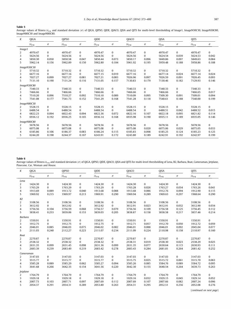
Table 5Average values of fitness Uavg and standard deviation ðrÞ of QIGA, QIPSO, QIDE, QIACO, QISA and QITS for multi-level thresholding of Image1, ImageN30C30, ImageN30C80,ImageN80C30 and ImageN80C80.


Uavg r Uavg r Uavg r Uavg r Uavg r Uavg r

Image12 4970.47 0 4970.47 0 4970.47 0 4970.47 0 4970.47 0 4970.47 03 5624.56 0 5624.56 0 5624.56 0 5624.56 0 5624.54 0.039 5624.53 0.0424 5850.30 0.050 5850.58 0.047 5850.44 0.073 5850.17 0.096 5849.86 0.097 5849.63 0.0845 5962.14 0.156 5962.89 0.150 5962.80 0.184 5961.92 0.195 5959.48 0.188 5958.86 0.188

ImageN30C302 5710.32 0 5710.32 0 5710.32 0 5710.32 0 5710.32 0 5710.32 03 6677.16 0 6677.16 0 6677.15 0.019 6677.16 0 6677.14 0.024 6677.14 0.0244 7027.27 0.099 7027.27 0.081 7027.21 0.083 7026.96 0.097 7026.59 0.091 7026.45 0.0935 7131.10 0.190 7131.24 0.116 7131.05 0.157 7130.83 0.179 7130.46 0.182 7129.93 0.146

ImageN30C802 7340.33 0 7340.33 0 7340.33 0 7340.33 0 7340.33 0 7340.33 03 7466.66 0 7466.66 0 7466.66 0 7466.66 0 7466.66 0 7466.65 0.0174 7510.20 0.096 7510.27 0.092 7510.10 0.089 7510.09 0.095 7509.30 0.091 7509.01 0.0945 7541.08 0.177 7541.73 0.152 7541.29 0.168 7541.28 0.118 7540.61 0.188 7540.00 0.199

ImageN80C302 5528.15 0 5528.15 0 5528.15 0 5528.15 0 5528.15 0 5528.15 03 6488.54 0 6488.54 0 6488.54 0 6488.54 0 6488.51 0.042 6488.52 0.0154 6822.23 0.094 6822.43 0.094 6822.36 0.072 6822.16 0.107 6822.18 0.095 6821.82 0.1145 6936.12 0.192 6936.25 0.165 6936.14 0.168 6935.98 0.190 6935.11 0.189 6935.05 0.146

ImageN80C802 5678.56 0 5678.56 0 5678.56 0 5678.56 0 5678.56 0 5678.56 03 6075.08 0 6075.08 0 6075.08 0 6075.08 0.020 6075.06 0.029 6075.05 0.0334 6185.86 0.106 6186.37 0.083 6186.24 0.115 6185.83 0.098 6185.25 0.124 6185.23 0.1255 6244.20 0.198 6244.37 0.167 6243.91 0.172 6243.80 0.189 6242.91 0.192 6242.97 0.199

Table 6Average values of fitness Uavg and standard deviation ðrÞ of QIGA, QIPSO, QIDE, QIACO, QISA and QITS for multi-level thresholding of Lena, B2, Barbara, Boat, Cameraman, Jetplane,Pinecone, Car, Woman and House.



Lena2 1424.30 0 1424.30 0 1424.30 0 1424.30 0 1424.30 0 1424.30 03 1763.29 0 1763.29 0 1763.29 0 1763.28 0.026 1763.27 0.034 1763.26 0.0414 1913.69 0.089 1913.72 0.040 1913.68 0.088 1913.68 0.086 1912.76 0.094 1912.90 0.1155 1969.92 0.215 1969.97 0.213 1969.91 0.290 1969.94 0.289 1969.63 0.297 1968.64 0.290

B22 3108.56 0 3108.56 0 3108.56 0 3108.56 0 3108.56 0 3108.56 03 3612.92 0 3612.92 0 3612.92 0 3612.91 0.023 3612.91 0.032 3612.90 0.0344 3756.56 0.104 3756.59 0.068 3756.57 0.079 3756.56 0.109 3756.58 0.125 3756.45 0.1125 3838.41 0.253 3839.06 0.153 3839.03 0.205 3838.87 0.158 3838.58 0.217 3837.46 0.214

Barbara2 1550.91 0 1550.91 0 1550.91 0 1550.91 0 1550.91 0 1550.91 03 1912.75 0 1912.75 0 1912.75 0 1912.71 0.057 1912.70 0.050 1912.72 0.0594 2046.01 0.085 2046.03 0.075 2046.02 0.082 2046.01 0.088 2046.01 0.092 2045.04 0.0775 2111.03 0.240 2112.27 0.223 2111.07 0.234 2111.09 0.224 2110.98 0.158 2110.97 0.160

Boat2 2270.87 0 2270.87 0 2270.87 0 2270.87 0 2270.87 0 2270.87 03 2538.32 0 2538.32 0 2538.32 0 2538.31 0.019 2538.30 0.023 2538.29 0.0254 2631.35 0.099 2631.45 0.098 2631.36 0.099 2631.35 0.077 2630.64 0.115 2630.93 0.1115 2683.39 0.239 2683.49 0.219 2683.42 0.278 2683.43 0.284 2681.81 0.264 2681.42 0.252

Cameraman2 3147.03 0 3147.03 0 3147.03 0 3147.03 0 3147.03 0 3147.03 03 3515.77 0 3515.77 0 3515.77 0 3515.75 0.025 3515.72 0.061 3515.70 0.0634 3585.28 0.089 3585.29 0.062 3585.27 0.094 3585.26 0.085 3584.76 0.089 3584.72 0.0955 3641.68 0.266 3642.35 0.154 3641.56 0.220 3642.30 0.155 3640.54 0.264 3639.73 0.263

Jetplane2 1764.79 0 1764.79 0 1764.79 0 1764.79 0 1764.79 0 1764.79 03 1929.18 0 1929.18 0 1929.18 0 1929.16 0.032 1929.15 0.045 1929.14 0.0524 2007.73 0.103 2007.71 0.097 2007.69 0.112 2007.69 0.107 2007.66 0.082 2007.24 0.0965 2054.37 0.291 2054.31 0.289 2053.80 0.263 2054.31 0.295 2052.51 0.256 2052.08 0.276

(continued on next page)


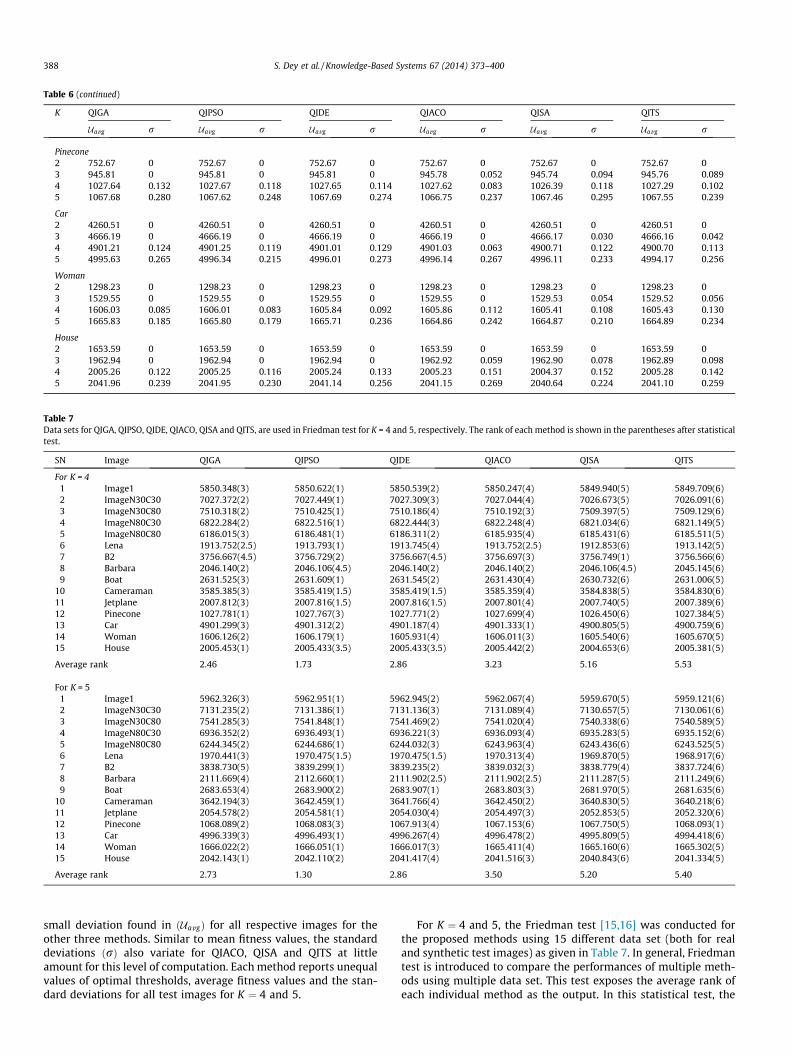
Table 6 (continued)



Pinecone2 752.67 0 752.67 0 752.67 0 752.67 0 752.67 0 752.67 03 945.81 0 945.81 0 945.81 0 945.78 0.052 945.74 0.094 945.76 0.0894 1027.64 0.132 1027.67 0.118 1027.65 0.114 1027.62 0.083 1026.39 0.118 1027.29 0.1025 1067.68 0.280 1067.62 0.248 1067.69 0.274 1066.75 0.237 1067.46 0.295 1067.55 0.239

Car2 4260.51 0 4260.51 0 4260.51 0 4260.51 0 4260.51 0 4260.51 03 4666.19 0 4666.19 0 4666.19 0 4666.19 0 4666.17 0.030 4666.16 0.0424 4901.21 0.124 4901.25 0.119 4901.01 0.129 4901.03 0.063 4900.71 0.122 4900.70 0.1135 4995.63 0.265 4996.34 0.215 4996.01 0.273 4996.14 0.267 4996.11 0.233 4994.17 0.256

Woman2 1298.23 0 1298.23 0 1298.23 0 1298.23 0 1298.23 0 1298.23 03 1529.55 0 1529.55 0 1529.55 0 1529.55 0 1529.53 0.054 1529.52 0.0564 1606.03 0.085 1606.01 0.083 1605.84 0.092 1605.86 0.112 1605.41 0.108 1605.43 0.1305 1665.83 0.185 1665.80 0.179 1665.71 0.236 1664.86 0.242 1664.87 0.210 1664.89 0.234

House2 1653.59 0 1653.59 0 1653.59 0 1653.59 0 1653.59 0 1653.59 03 1962.94 0 1962.94 0 1962.94 0 1962.92 0.059 1962.90 0.078 1962.89 0.0984 2005.26 0.122 2005.25 0.116 2005.24 0.133 2005.23 0.151 2004.37 0.152 2005.28 0.1425 2041.96 0.239 2041.95 0.230 2041.14 0.256 2041.15 0.269 2040.64 0.224 2041.10 0.259

Table 7Data sets for QIGA, QIPSO, QIDE, QIACO, QISA and QITS, are used in Friedman test for K = 4 and 5, respectively. The rank of each method is shown in the parentheses after statisticaltest.

SN Image QIGA QIPSO QIDE QIACO QISA QITS

For K = 41 Image1 5850.348(3) 5850.622(1) 5850.539(2) 5850.247(4) 5849.940(5) 5849.709(6)2 ImageN30C30 7027.372(2) 7027.449(1) 7027.309(3) 7027.044(4) 7026.673(5) 7026.091(6)3 ImageN30C80 7510.318(2) 7510.425(1) 7510.186(4) 7510.192(3) 7509.397(5) 7509.129(6)4 ImageN80C30 6822.284(2) 6822.516(1) 6822.444(3) 6822.248(4) 6821.034(6) 6821.149(5)5 ImageN80C80 6186.015(3) 6186.481(1) 6186.311(2) 6185.935(4) 6185.431(6) 6185.511(5)6 Lena 1913.752(2.5) 1913.793(1) 1913.745(4) 1913.752(2.5) 1912.853(6) 1913.142(5)7 B2 3756.667(4.5) 3756.729(2) 3756.667(4.5) 3756.697(3) 3756.749(1) 3756.566(6)8 Barbara 2046.140(2) 2046.106(4.5) 2046.140(2) 2046.140(2) 2046.106(4.5) 2045.145(6)9 Boat 2631.525(3) 2631.609(1) 2631.545(2) 2631.430(4) 2630.732(6) 2631.006(5)

10 Cameraman 3585.385(3) 3585.419(1.5) 3585.419(1.5) 3585.359(4) 3584.838(5) 3584.830(6)11 Jetplane 2007.812(3) 2007.816(1.5) 2007.816(1.5) 2007.801(4) 2007.740(5) 2007.389(6)12 Pinecone 1027.781(1) 1027.767(3) 1027.771(2) 1027.699(4) 1026.450(6) 1027.384(5)13 Car 4901.299(3) 4901.312(2) 4901.187(4) 4901.333(1) 4900.805(5) 4900.759(6)14 Woman 1606.126(2) 1606.179(1) 1605.931(4) 1606.011(3) 1605.540(6) 1605.670(5)15 House 2005.453(1) 2005.433(3.5) 2005.433(3.5) 2005.442(2) 2004.653(6) 2005.381(5)

Average rank 2.46 1.73 2.86 3.23 5.16 5.53

For K = 51 Image1 5962.326(3) 5962.951(1) 5962.945(2) 5962.067(4) 5959.670(5) 5959.121(6)2 ImageN30C30 7131.235(2) 7131.386(1) 7131.136(3) 7131.089(4) 7130.657(5) 7130.061(6)3 ImageN30C80 7541.285(3) 7541.848(1) 7541.469(2) 7541.020(4) 7540.338(6) 7540.589(5)4 ImageN80C30 6936.352(2) 6936.493(1) 6936.221(3) 6936.093(4) 6935.283(5) 6935.152(6)5 ImageN80C80 6244.345(2) 6244.686(1) 6244.032(3) 6243.963(4) 6243.436(6) 6243.525(5)6 Lena 1970.441(3) 1970.475(1.5) 1970.475(1.5) 1970.313(4) 1969.870(5) 1968.917(6)7 B2 3838.730(5) 3839.299(1) 3839.235(2) 3839.032(3) 3838.779(4) 3837.724(6)8 Barbara 2111.669(4) 2112.660(1) 2111.902(2.5) 2111.902(2.5) 2111.287(5) 2111.249(6)9 Boat 2683.653(4) 2683.900(2) 2683.907(1) 2683.803(3) 2681.970(5) 2681.635(6)

10 Cameraman 3642.194(3) 3642.459(1) 3641.766(4) 3642.450(2) 3640.830(5) 3640.218(6)11 Jetplane 2054.578(2) 2054.581(1) 2054.030(4) 2054.497(3) 2052.853(5) 2052.320(6)12 Pinecone 1068.089(2) 1068.083(3) 1067.913(4) 1067.153(6) 1067.750(5) 1068.093(1)13 Car 4996.339(3) 4996.493(1) 4996.267(4) 4996.478(2) 4995.809(5) 4994.418(6)14 Woman 1666.022(2) 1666.051(1) 1666.017(3) 1665.411(4) 1665.160(6) 1665.302(5)15 House 2042.143(1) 2042.110(2) 2041.417(4) 2041.516(3) 2040.843(6) 2041.334(5)

Average rank 2.73 1.30 2.86 3.50 5.20 5.40


small deviation found in ðUavgÞ for all respective images for theother three methods. Similar to mean fitness values, the standarddeviations ðrÞ also variate for QIACO, QISA and QITS at littleamount for this level of computation. Each method reports unequalvalues of optimal thresholds, average fitness values and the stan-dard deviations for all test images for K ¼ 4 and 5.

For K ¼ 4 and 5, the Friedman test [15,16] was conducted forthe proposed methods using 15 different data set (both for realand synthetic test images) as given in Table 7. In general, Friedmantest is introduced to compare the performances of multiple meth-ods using multiple data set. This test exposes the average rank ofeach individual method as the output. In this statistical test, the

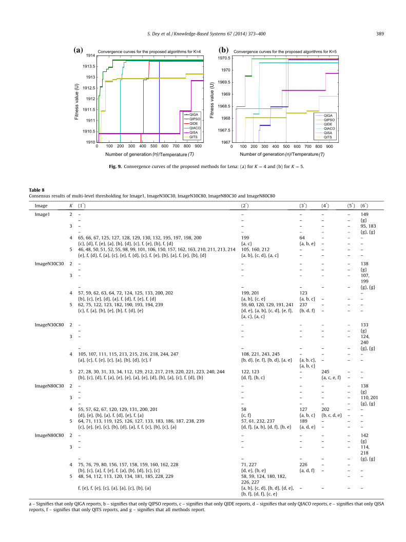
Table 8Consensus results of multi-level thresholding for Image1, ImageN30C30, ImageN30C80, ImageN80C30 and ImageN80C80

Image K (1*) (2*) (3*) (4*) (5*) (6*)

Image1 2 – – – – – 149– – – – – {g}

3 – – – – – 95, 183– – – – – {g}, {g}

4 65, 66, 67, 125, 127, 128, 129, 130, 132, 195, 197, 198, 200 199 64 – – –{c}, {d}, f, {e}, {a}, {b}, {d}, {c}, f, {e}, {b}, f, {d} {a, c} {a, b, e} – – –

5 46, 48, 50, 51, 52, 55, 98, 99, 101, 106, 150, 157, 162, 163, 210, 211, 213, 214 105, 160, 212 – – – –{e}, f, {d}, f, {a}, {c}, {e}, f, {d}, {c}, f, {e}, {b}, {a}, f, {e}, {b}, {d} {a, b}, {c, d}, {a, c} – – – –

ImageN30C30 2 – – – – – 138– – – – – {g}

3 – – – – – 107,199

– – – – – {g}, {g}4 57, 59, 62, 63, 64, 72, 124, 125, 133, 200, 202 199, 201 123 –

{b}, {c}, {e}, {d}, {a}, f, {d}, f, {e}, f, {d} {a, b}, {c, e} {a, b, c} – – –5 62, 75, 122, 123, 182, 190, 193, 194, 239 59, 60, 120, 129, 191, 241 237 – – –

{c}, f, {a}, {b}, {e}, {b}, f, {d}, {e} {d, e}, {a, b}, {c, d}, {e, f},{a, c}, {a, c}

{b, d, f} – – –

ImageN30C80 2 – – – – – 133– – – – – {g}

3 – – – – – 124,240

– – – – – {g}, {g}4 105, 107, 111, 115, 213, 215, 216, 218, 244, 247 108, 221, 243, 245 – – – –

{a}, {c}, f, {e}, {c}, {a}, {b}, {d}, {c}, f {b, d}, {e, f}, {b, d}, {a, e} {a, b, c},{a, b, c}

– – –

5 27, 28, 30, 31, 33, 34, 112, 129, 212, 217, 219, 220, 221, 223, 240, 244 122, 123 – 245 – –{b}, {c}, {d}, f, {a}, {e}, {e}, {a}, {e}, {d}, {b}, {a}, {c}, f, {d}, {b} {d, f}, {b, c} – {a, c, e, f} – –

ImageN80C30 2 – – – – – 138– – – – – {g}

3 – – – – – 110, 201– – – – – {g}, {g}

4 55, 57, 62, 67, 120, 129, 131, 200, 201 58 127 202 – –{d}, {e}, {b}, {a}, f, {d}, {e}, f, {a} {c, f} {a, b, c} {b, c, d, e} – –

5 64, 71, 113, 119, 125, 126, 127, 133, 183, 186, 187, 238, 239 57, 61, 232, 237 189 – – –{c}, {e}, {e}, {c}, {b}, {d}, {a}, f, f, {c}, {b}, {c}, {a} {d, f}, {a, b}, {d, f}, {b, e} {a, d, e} – – –

ImageN80C80 2 – – – – – 142– – – – – {g}

3 – – – – – 114,218

– – – – – {g}, {g}4 75, 76, 79, 80, 156, 157, 158, 159, 160, 162, 228 71, 227 226 – –

{b}, {c}, {a}, f, {e}, f, {a}, {b}, {d}, {c}, {c} {d, e}, {b, e} {a, d, f} – – –5 48, 54, 112, 113, 120, 134, 181, 185, 228, 229 58, 59, 124, 180, 182,

226, 227– –

f, {e}, f, {e}, {c}, {a}, {a}, {c}, {b}, {a} {a, b}, {c, d}, {b, d}, {d, e},{b, f}, {d, f}, {c, e}

– – – –

a – Signifies that only QIGA reports, b – signifies that only QIPSO reports, c – signifies that only QIDE reports, d – signifies that only QIACO reports, e – signifies that only QISAreports, f – signifies that only QITS reports, and g – signifies that all methods report.

0 100 200 300 400 500 600 700 800 9001910

1910.5

1911

1911.5

1912

1912.5

1913

1913.5

1914

Number of generation

Fitn

ess

valu

e (U

)

Convergence curves for the proposed algorithms for K=4

QIGAQIPSOQIDEQIACOQISAQITS

(n)/Temperature (T)

(a)

0 100 200 300 400 500 600 700 800 9001967

1967.5

1968

1968.5

1969

1969.5

1970

1970.5Convergence curves for the proposed algorithms for K=5

Fitn

ess

valu

e (U

)

QIGAQIPSOQIDEQIACOQISAQITS

(T)Number of generation /Temperature(n)

(b)

Fig. 9. Convergence curves of the proposed methods for Lena: (a) for K ¼ 4 and (b) for K ¼ 5.


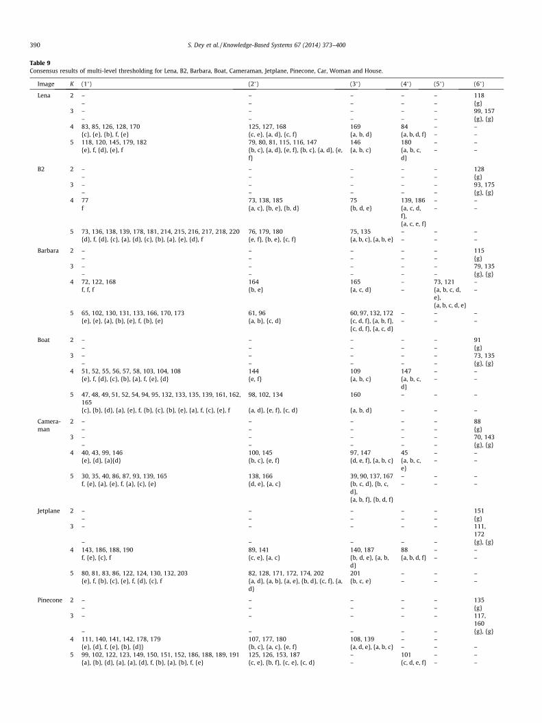
Table 9Consensus results of multi-level thresholding for Lena, B2, Barbara, Boat, Cameraman, Jetplane, Pinecone, Car, Woman and House.

Image K (1�) (2�) (3�) (4�) (5�) (6�)

Lena 2 – – – – – 118– – – – – {g}

3 – – – – – 99, 157– – – – – {g}, {g}

4 83, 85, 126, 128, 170 125, 127, 168 169 84 – –{c}, {e}, {b}, f, {e} {c, e}, {a, d}, {c, f} {a, b, d} {a, b, d, f} – –

5 118, 120, 145, 179, 182 79, 80, 81, 115, 116, 147 146 180 – –{e}, f, {d}, {e}, f {b, c}, {a, d}, {e, f}, {b, c}, {a, d}, {e,

f}{a, b, c} {a, b, c,

d}– –

B2 2 – – – – – 128– – – – – {g}

3 – – – – – 93, 175– – – – – {g}, {g}

4 77 73, 138, 185 75 139, 186 – –f {a, c}, {b, e}, {b, d} {b, d, e} {a, c, d,

f},{a, c, e, f}

– –

5 73, 136, 138, 139, 178, 181, 214, 215, 216, 217, 218, 220 76, 179, 180 75, 135 – – –{d}, f, {d}, {c}, {a}, {d}, {c}, {b}, {a}, {e}, {d}, f {e, f}, {b, e}, {c, f} {a, b, c}, {a, b, e} – – –

Barbara 2 – – – – – 115– – – – – {g}

3 – – – – – 79, 135– – – – – {g}, {g}

4 72, 122, 168 164 165 – 73, 121 –f, f, f {b, e} {a, c, d} – {a, b, c, d,

e},{a, b, c, d, e}

–

5 65, 102, 130, 131, 133, 166, 170, 173 61, 96 60, 97, 132, 172 – – –{e}, {e}, {a}, {b}, {e}, f, {b}, {e} {a, b}, {c, d} {c, d, f}, {a, b, f},

{c, d, f}, {a, c, d}– – –

Boat 2 – – – – – 91– – – – – {g}

3 – – – – – 73, 135– – – – – {g}, {g}

4 51, 52, 55, 56, 57, 58, 103, 104, 108 144 109 147 – –{e}, f, {d}, {c}, {b}, {a}, f, {e}, {d} {e, f} {a, b, c} {a, b, c,

d}– –

5 47, 48, 49, 51, 52, 54, 94, 95, 132, 133, 135, 139, 161, 162,165

98, 102, 134 160 – – –

{c}, {b}, {d}, {a}, {e}, f, {b}, {c}, {b}, {e}, {a}, f, {c}, {e}, f {a, d}, {e, f}, {c, d} {a, b, d} – – –

Camera- 2 – – – – – 88man – – – – – {g}

3 – – – – – 70, 143– – – – – {g}, {g}

4 40, 43, 99, 146 100, 145 97, 147 45 – –{e}, {d}, {a}{d} {b, c}, {e, f} {d, e, f}, {a, b, c} {a, b, c,

e}– –

5 30, 35, 40, 86, 87, 93, 139, 165 138, 166 39, 90, 137, 167 – – –f, {e}, {a}, {e}, f, {a}, {c}, {e} {d, e}, {a, c} {b, c, d}, {b, c,

d},{a, b, f}, {b, d, f}

– – –

Jetplane 2 – – – – – 151– – – – – {g}

3 – – – – – 111,172

– – – – – {g}, {g}4 143, 186, 188, 190 89, 141 140, 187 88 – –

f, {e}, {c}, f {c, e}, {a, c} {b, d, e}, {a, b,d}

{a, b, d, f} – –

5 80, 81, 83, 86, 122, 124, 130, 132, 203 82, 128, 171, 172, 174, 202 201 – – –{e}, f, {b}, {c}, {e}, f, {d}, {c}, f {a, d}, {a, b}, {a, e}, {b, d}, {c, f}, {a,

d}{b, c, e} – – –

Pinecone 2 – – – – – 135– – – – – {g}

3 – – – – – 117,160

– – – – – {g}, {g}4 111, 140, 141, 142, 178, 179 107, 177, 180 108, 139 – –

{e}, {d}, f, {e}, {b}, {d}} {b, c}, {a, c}, {e, f} {a, d, e}, {a, b, c} – – –5 99, 102, 122, 123, 149, 150, 151, 152, 186, 188, 189, 191 125, 126, 153, 187 – 101 – –

{a}, {b}, {d}, {a}, {a}, {d}, f, {b}, {a}, {b}, f, {e} {c, e}, {b, f}, {c, e}, {c, d} – {c, d, e, f} – –


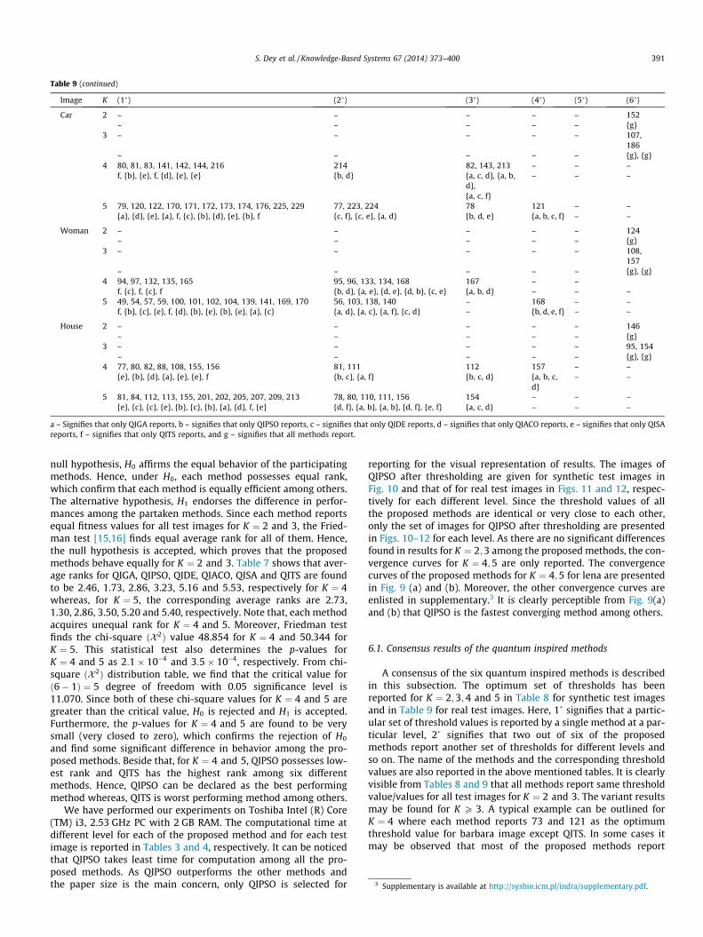
Table 9 (continued)

Image K (1�) (2�) (3�) (4�) (5�) (6�)

Car 2 – – – – – 152– – – – – {g}

3 – – – – – 107,186

– – – – – {g}, {g}4 80, 81, 83, 141, 142, 144, 216 214 82, 143, 213 – – –

f, {b}, {e}, f, {d}, {e}, {e} {b, d} {a, c, d}, {a, b,d},{a, c, f}

– – –

5 79, 120, 122, 170, 171, 172, 173, 174, 176, 225, 229 77, 223, 224 78 121 – –{a}, {d}, {e}, {a}, f, {c}, {b}, {d}, {e}, {b}, f {c, f}, {c, e}, {a, d} {b, d, e} {a, b, c, f} – –

Woman 2 – – – – – 124– – – – – {g}

3 – – – – – 108,157

– – – – – {g}, {g}4 94, 97, 132, 135, 165 95, 96, 133, 134, 168 167 – –

f, {c}, f, {c}, f {b, d}, {a, e}, {d, e}, {d, b}, {c, e} {a, b, d} – – –5 49, 54, 57, 59, 100, 101, 102, 104, 139, 141, 169, 170 56, 103, 138, 140 – 168 – –

f, {b}, {c}, {e}, f, {d}, {b}, {e}, {b}, {e}, {a}, {c} {a, d}, {a, c}, {a, f}, {c, d} – {b, d, e, f} – –

House 2 – – – – – 146– – – – – {g}

3 – – – – – 95, 154– – – – – {g}, {g}

4 77, 80, 82, 88, 108, 155, 156 81, 111 112 157 – –{e}, {b}, {d}, {a}, {e}, {e}, f {b, c}, {a, f} {b, c, d} {a, b, c,

d}– –

5 81, 84, 112, 113, 155, 201, 202, 205, 207, 209, 213 78, 80, 110, 111, 156 154 – – –{e}, {c}, {c}, {e}, {b}, {c}, {b}, {a}, {d}, f, {e} {d, f}, {a, b}, {a, b}, {d, f}, {e, f} {a, c, d} – – –

a – Signifies that only QIGA reports, b – signifies that only QIPSO reports, c – signifies that only QIDE reports, d – signifies that only QIACO reports, e – signifies that only QISAreports, f – signifies that only QITS reports, and g – signifies that all methods report.

3 Supplementary is available at http://sysbio.icm.pl/indra/supplementary.pdf.


null hypothesis, H0 affirms the equal behavior of the participatingmethods. Hence, under H0, each method possesses equal rank,which confirm that each method is equally efficient among others.The alternative hypothesis, H1 endorses the difference in perfor-mances among the partaken methods. Since each method reportsequal fitness values for all test images for K ¼ 2 and 3, the Fried-man test [15,16] finds equal average rank for all of them. Hence,the null hypothesis is accepted, which proves that the proposedmethods behave equally for K ¼ 2 and 3. Table 7 shows that aver-age ranks for QIGA, QIPSO, QIDE, QIACO, QISA and QITS are foundto be 2.46, 1.73, 2.86, 3.23, 5.16 and 5.53, respectively for K ¼ 4whereas, for K ¼ 5, the corresponding average ranks are 2.73,1.30, 2.86, 3.50, 5.20 and 5.40, respectively. Note that, each methodacquires unequal rank for K ¼ 4 and 5. Moreover, Friedman testfinds the chi-square ðX2Þ value 48.854 for K ¼ 4 and 50.344 forK ¼ 5. This statistical test also determines the p-values forK ¼ 4 and 5 as 2:1� 10�4 and 3:5� 10�4, respectively. From chi-square ðX2Þ distribution table, we find that the critical value forð6� 1Þ ¼ 5 degree of freedom with 0.05 significance level is11.070. Since both of these chi-square values for K ¼ 4 and 5 aregreater than the critical value, H0 is rejected and H1 is accepted.Furthermore, the p-values for K ¼ 4 and 5 are found to be verysmall (very closed to zero), which confirms the rejection of H0

and find some significant difference in behavior among the pro-posed methods. Beside that, for K ¼ 4 and 5, QIPSO possesses low-est rank and QITS has the highest rank among six differentmethods. Hence, QIPSO can be declared as the best performingmethod whereas, QITS is worst performing method among others.

We have performed our experiments on Toshiba Intel (R) Core(TM) i3, 2.53 GHz PC with 2 GB RAM. The computational time atdifferent level for each of the proposed method and for each testimage is reported in Tables 3 and 4, respectively. It can be noticedthat QIPSO takes least time for computation among all the pro-posed methods. As QIPSO outperforms the other methods andthe paper size is the main concern, only QIPSO is selected for

reporting for the visual representation of results. The images ofQIPSO after thresholding are given for synthetic test images inFig. 10 and that of for real test images in Figs. 11 and 12, respec-tively for each different level. Since the threshold values of allthe proposed methods are identical or very close to each other,only the set of images for QIPSO after thresholding are presentedin Figs. 10–12 for each level. As there are no significant differencesfound in results for K ¼ 2;3 among the proposed methods, the con-vergence curves for K ¼ 4;5 are only reported. The convergencecurves of the proposed methods for K ¼ 4;5 for lena are presentedin Fig. 9 (a) and (b). Moreover, the other convergence curves areenlisted in supplementary.3 It is clearly perceptible from Fig. 9(a)and (b) that QIPSO is the fastest converging method among others.

6.1. Consensus results of the quantum inspired methods

A consensus of the six quantum inspired methods is describedin this subsection. The optimum set of thresholds has beenreported for K ¼ 2;3;4 and 5 in Table 8 for synthetic test imagesand in Table 9 for real test images. Here, 1� signifies that a partic-ular set of threshold values is reported by a single method at a par-ticular level, 2� signifies that two out of six of the proposedmethods report another set of thresholds for different levels andso on. The name of the methods and the corresponding thresholdvalues are also reported in the above mentioned tables. It is clearlyvisible from Tables 8 and 9 that all methods report same thresholdvalue/values for all test images for K ¼ 2 and 3. The variant resultsmay be found for K P 3. A typical example can be outlined forK ¼ 4 where each method reports 73 and 121 as the optimumthreshold value for barbara image except QITS. In some cases itmay be observed that most of the proposed methods report

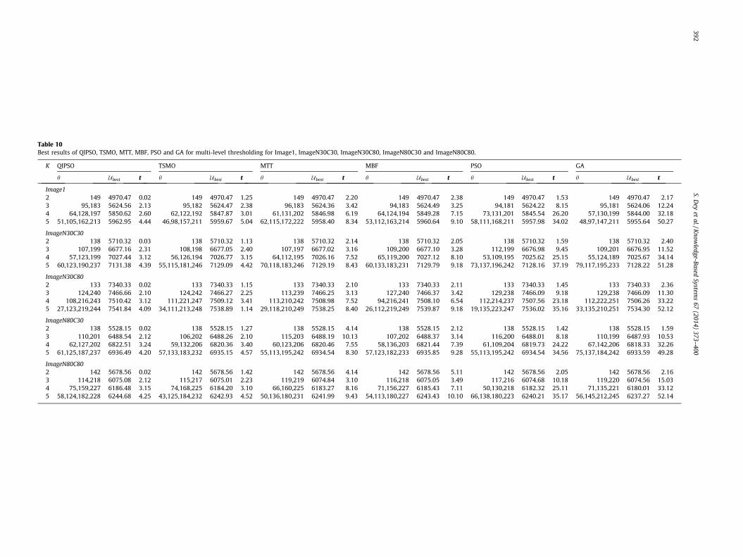
http://sysbio.icm.pl/indra/supplementary.pdf

Table 10Best results of QIPSO, TSMO, MTT, MBF, PSO and GA for multi-level thresholding for Image1, ImageN30C30, ImageN30C80, ImageN80C30 and ImageN80C80.

K QIPSO TSMO MTT MBF PSO GA


Image12 149 4970.47 0.02 149 4970.47 1.25 149 4970.47 2.20 149 4970.47 2.38 149 4970.47 1.53 149 4970.47 2.173 95,183 5624.56 2.13 95,182 5624.47 2.38 96,183 5624.36 3.42 94,183 5624.49 3.25 94,181 5624.22 8.15 95,181 5624.06 12.244 64,128,197 5850.62 2.60 62,122,192 5847.87 3.01 61,131,202 5846.98 6.19 64,124,194 5849.28 7.15 73,131,201 5845.54 26.20 57,130,199 5844.00 32.185 51,105,162,213 5962.95 4.44 46,98,157,211 5959.67 5.04 62,115,172,222 5958.40 8.34 53,112,163,214 5960.64 9.10 58,111,168,211 5957.98 34.02 48,97,147,211 5955.64 50.27

ImageN30C302 138 5710.32 0.03 138 5710.32 1.13 138 5710.32 2.14 138 5710.32 2.05 138 5710.32 1.59 138 5710.32 2.403 107,199 6677.16 2.31 108,198 6677.05 2.40 107,197 6677.02 3.16 109,200 6677.10 3.28 112,199 6676.98 9.45 109,201 6676.95 11.524 57,123,199 7027.44 3.12 56,126,194 7026.77 3.15 64,112,195 7026.16 7.52 65,119,200 7027.12 8.10 53,109,195 7025.62 25.15 55,124,189 7025.67 34.145 60,123,190,237 7131.38 4.39 55,115,181,246 7129.09 4.42 70,118,183,246 7129.19 8.43 60,133,183,231 7129.79 9.18 73,137,196,242 7128.16 37.19 79,117,195,233 7128.22 51.28

ImageN30C802 133 7340.33 0.02 133 7340.33 1.15 133 7340.33 2.10 133 7340.33 2.11 133 7340.33 1.45 133 7340.33 2.363 124,240 7466.66 2.10 124,242 7466.27 2.25 113,239 7466.25 3.13 127,240 7466.37 3.42 129,238 7466.09 9.18 129,238 7466.09 11.304 108,216,243 7510.42 3.12 111,221,247 7509.12 3.41 113,210,242 7508.98 7.52 94,216,241 7508.10 6.54 112,214,237 7507.56 23.18 112,222,251 7506.26 33.225 27,123,219,244 7541.84 4.09 34,111,213,248 7538.89 1.14 29,118,210,249 7538.25 8.40 26,112,219,249 7539.87 9.18 19,135,223,247 7536.02 35.16 33,135,210,251 7534.30 52.12

ImageN80C302 138 5528.15 0.02 138 5528.15 1.27 138 5528.15 4.14 138 5528.15 2.12 138 5528.15 1.42 138 5528.15 1.593 110,201 6488.54 2.12 106,202 6488.26 2.10 115,203 6488.19 10.13 107,202 6488.37 3.14 116,200 6488.01 8.18 110,199 6487.93 10.534 62,127,202 6822.51 3.24 59,132,206 6820.36 3.40 60,123,206 6820.46 7.55 58,136,203 6821.44 7.39 61,109,204 6819.73 24.22 67,142,206 6818.33 32.265 61,125,187,237 6936.49 4.20 57,133,183,232 6935.15 4.57 55,113,195,242 6934.54 8.30 57,123,182,233 6935.85 9.28 55,113,195,242 6934.54 34.56 75,137,184,242 6933.59 49.28

ImageN80C802 142 5678.56 0.02 142 5678.56 1.42 142 5678.56 4.14 142 5678.56 5.11 142 5678.56 2.05 142 5678.56 2.163 114,218 6075.08 2.12 115,217 6075.01 2.23 119,219 6074.84 3.10 116,218 6075.05 3.49 117,216 6074.68 10.18 119,220 6074.56 15.034 75,159,227 6186.48 3.15 74,168,225 6184.20 3.10 66,160,225 6183.27 8.16 71,156,227 6185.43 7.11 50,130,218 6182.32 25.11 71,135,221 6180.01 33.125 58,124,182,228 6244.68 4.25 43,125,184,232 6242.93 4.52 50,136,180,231 6241.99 9.43 54,113,180,227 6243.43 10.10 66,138,180,223 6240.21 35.17 56,145,212,245 6237.27 52.14

392S.D

eyet

al./Know

ledge-BasedSystem

s67

(2014)373–

400

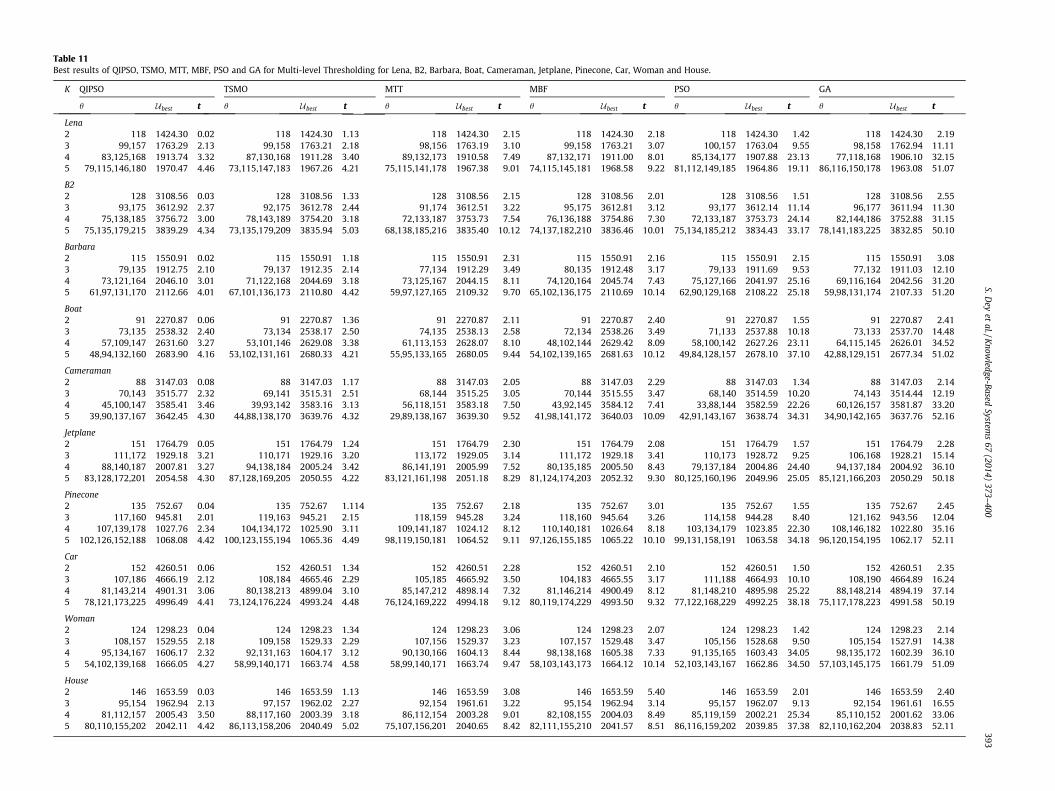
Table 11Best results of QIPSO, TSMO, MTT, MBF, PSO and GA for Multi-level Thresholding for Lena, B2, Barbara, Boat, Cameraman, Jetplane, Pinecone, Car, Woman and House.


h Ubest t h Ubest t h Ubest t h Ubest t h best t h Ubest t

Lena2 118 1424.30 0.02 118 1424.30 1.13 118 1424.30 2.15 118 1424.30 2.18 118 24.30 1.42 118 1424.30 2.193 99,157 1763.29 2.13 99,158 1763.21 2.18 98,156 1763.19 3.10 99,158 1763.21 3.07 100,157 63.04 9.55 98,158 1762.94 11.114 83,125,168 1913.74 3.32 87,130,168 1911.28 3.40 89,132,173 1910.58 7.49 87,132,171 1911.00 8.01 85,134,177 07.88 23.13 77,118,168 1906.10 32.155 79,115,146,180 1970.47 4.46 73,115,147,183 1967.26 4.21 75,115,141,178 1967.38 9.01 74,115,145,181 1968.58 9.22 81,112,149,185 64.86 19.11 86,116,150,178 1963.08 51.07

B22 128 3108.56 0.03 128 3108.56 1.33 128 3108.56 2.15 128 3108.56 2.01 128 08.56 1.51 128 3108.56 2.553 93,175 3612.92 2.37 92,175 3612.78 2.44 91,174 3612.51 3.22 95,175 3612.81 3.12 93,177 12.14 11.14 96,177 3611.94 11.304 75,138,185 3756.72 3.00 78,143,189 3754.20 3.18 72,133,187 3753.73 7.54 76,136,188 3754.86 7.30 72,133,187 53.73 24.14 82,144,186 3752.88 31.155 75,135,179,215 3839.29 4.34 73,135,179,209 3835.94 5.03 68,138,185,216 3835.40 10.12 74,137,182,210 3836.46 10.01 75,134,185,212 34.43 33.17 78,141,183,225 3832.85 50.10

Barbara2 115 1550.91 0.02 115 1550.91 1.18 115 1550.91 2.31 115 1550.91 2.16 115 50.91 2.15 115 1550.91 3.083 79,135 1912.75 2.10 79,137 1912.35 2.14 77,134 1912.29 3.49 80,135 1912.48 3.17 79,133 11.69 9.53 77,132 1911.03 12.104 73,121,164 2046.10 3.01 71,122,168 2044.69 3.18 73,125,167 2044.15 8.11 74,120,164 2045.74 7.43 75,127,166 41.97 25.16 69,116,164 2042.56 31.205 61,97,131,170 2112.66 4.01 67,101,136,173 2110.80 4.42 59,97,127,165 2109.32 9.70 65,102,136,175 2110.69 10.14 62,90,129,168 08.22 25.18 59,98,131,174 2107.33 51.20

Boat2 91 2270.87 0.06 91 2270.87 1.36 91 2270.87 2.11 91 2270.87 2.40 91 70.87 1.55 91 2270.87 2.413 73,135 2538.32 2.40 73,134 2538.17 2.50 74,135 2538.13 2.58 72,134 2538.26 3.49 71,133 37.88 10.18 73,133 2537.70 14.484 57,109,147 2631.60 3.27 53,101,146 2629.08 3.38 61,113,153 2628.07 8.10 48,102,144 2629.42 8.09 58,100,142 27.26 23.11 64,115,145 2626.01 34.525 48,94,132,160 2683.90 4.16 53,102,131,161 2680.33 4.21 55,95,133,165 2680.05 9.44 54,102,139,165 2681.63 10.12 49,84,128,157 78.10 37.10 42,88,129,151 2677.34 51.02

Cameraman2 88 3147.03 0.08 88 3147.03 1.17 88 3147.03 2.05 88 3147.03 2.29 88 47.03 1.34 88 3147.03 2.143 70,143 3515.77 2.32 69,141 3515.31 2.51 68,144 3515.25 3.05 70,144 3515.55 3.47 68,140 14.59 10.20 74,143 3514.44 12.194 45,100,147 3585.41 3.46 39,93,142 3583.16 3.13 56,118,151 3583.18 7.50 43,92,145 3584.12 7.41 33,88,144 82.59 22.26 60,126,157 3581.87 33.205 39,90,137,167 3642.45 4.30 44,88,138,170 3639.76 4.32 29,89,138,167 3639.30 9.52 41,98,141,172 3640.03 10.09 42,91,143,167 38.74 34.31 34,90,142,165 3637.76 52.16

Jetplane2 151 1764.79 0.05 151 1764.79 1.24 151 1764.79 2.30 151 1764.79 2.08 151 64.79 1.57 151 1764.79 2.283 111,172 1929.18 3.21 110,171 1929.16 3.20 113,172 1929.05 3.14 111,172 1929.18 3.41 110,173 28.72 9.25 106,168 1928.21 15.144 88,140,187 2007.81 3.27 94,138,184 2005.24 3.42 86,141,191 2005.99 7.52 80,135,185 2005.50 8.43 79,137,184 04.86 24.40 94,137,184 2004.92 36.105 83,128,172,201 2054.58 4.30 87,128,169,205 2050.55 4.22 83,121,161,198 2051.18 8.29 81,124,174,203 2052.32 9.30 80,125,160,196 49.96 25.05 85,121,166,203 2050.29 50.18

Pinecone2 135 752.67 0.04 135 752.67 1.114 135 752.67 2.18 135 752.67 3.01 135 2.67 1.55 135 752.67 2.453 117,160 945.81 2.01 119,163 945.21 2.15 118,159 945.28 3.24 118,160 945.64 3.26 114,158 4.28 8.40 121,162 943.56 12.044 107,139,178 1027.76 2.34 104,134,172 1025.90 3.11 109,141,187 1024.12 8.12 110,140,181 1026.64 8.18 103,134,179 23.85 22.30 108,146,182 1022.80 35.165 102,126,152,188 1068.08 4.42 100,123,155,194 1065.36 4.49 98,119,150,181 1064.52 9.11 97,126,155,185 1065.22 10.10 99,131,158,191 63.58 34.18 96,120,154,195 1062.17 52.11

Car2 152 4260.51 0.06 152 4260.51 1.34 152 4260.51 2.28 152 4260.51 2.10 152 60.51 1.50 152 4260.51 2.353 107,186 4666.19 2.12 108,184 4665.46 2.29 105,185 4665.92 3.50 104,183 4665.55 3.17 111,188 64.93 10.10 108,190 4664.89 16.244 81,143,214 4901.31 3.06 80,138,213 4899.04 3.10 85,147,212 4898.14 7.32 81,146,214 4900.49 8.12 81,148,210 95.98 25.22 88,148,214 4894.19 37.145 78,121,173,225 4996.49 4.41 73,124,176,224 4993.24 4.48 76,124,169,222 4994.18 9.12 80,119,174,229 4993.50 9.32 77,122,168,229 92.25 38.18 75,117,178,223 4991.58 50.19

Woman2 124 1298.23 0.04 124 1298.23 1.34 124 1298.23 3.06 124 1298.23 2.07 124 98.23 1.42 124 1298.23 2.143 108,157 1529.55 2.18 109,158 1529.33 2.29 107,156 1529.37 3.23 107,157 1529.48 3.47 105,156 28.68 9.50 105,154 1527.91 14.384 95,134,167 1606.17 2.32 92,131,163 1604.17 3.12 90,130,166 1604.13 8.44 98,138,168 1605.38 7.33 91,135,165 03.43 34.05 98,135,172 1602.39 36.105 54,102,139,168 1666.05 4.27 58,99,140,171 1663.74 4.58 58,99,140,171 1663.74 9.47 58,103,143,173 1664.12 10.14 52,103,143,167 62.86 34.50 57,103,145,175 1661.79 51.09

House2 146 1653.59 0.03 146 1653.59 1.13 146 1653.59 3.08 146 1653.59 5.40 146 53.59 2.01 146 1653.59 2.403 95,154 1962.94 2.13 97,157 1962.02 2.27 92,154 1961.61 3.22 95,154 1962.94 3.14 95,157 62.07 9.13 92,154 1961.61 16.554 81,112,157 2005.43 3.50 88,117,160 2003.39 3.18 86,112,154 2003.28 9.01 82,108,155 2004.03 8.49 85,119,159 02.21 25.34 85,110,152 2001.62 33.065 80,110,155,202 2042.11 4.42 86,113,158,206 2040.49 5.02 75,107,156,201 2040.65 8.42 82,111,155,210 2041.57 8.51 86,116,159,202 39.85 37.38 82,110,162,204 2038.83 52.11

S.Dey

etal./K

nowledge-Based

Systems

67(2014)

373–400

393

U

14171919

31363738

15192021

22252626

31353536

17192020

75941010

42464849

12151616

16192020

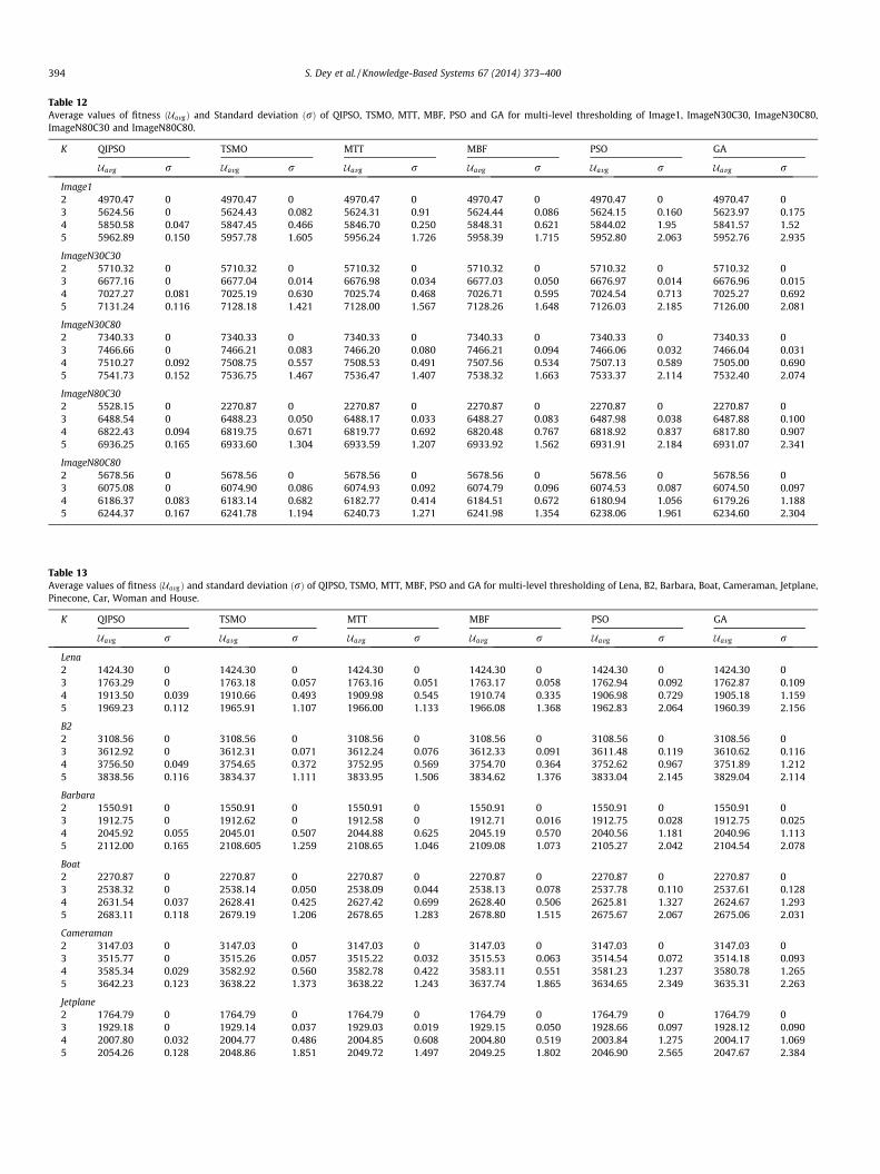
Table 13Average values of fitness ðUavgÞ and standard deviation ðrÞ of QIPSO, TSMO, MTT, MBF, PSO and GA for multi-level thresholding of Lena, B2, Barbara, Boat, Cameraman, Jetplane,Pinecone, Car, Woman and House.



Lena2 1424.30 0 1424.30 0 1424.30 0 1424.30 0 1424.30 0 1424.30 03 1763.29 0 1763.18 0.057 1763.16 0.051 1763.17 0.058 1762.94 0.092 1762.87 0.1094 1913.50 0.039 1910.66 0.493 1909.98 0.545 1910.74 0.335 1906.98 0.729 1905.18 1.1595 1969.23 0.112 1965.91 1.107 1966.00 1.133 1966.08 1.368 1962.83 2.064 1960.39 2.156

B22 3108.56 0 3108.56 0 3108.56 0 3108.56 0 3108.56 0 3108.56 03 3612.92 0 3612.31 0.071 3612.24 0.076 3612.33 0.091 3611.48 0.119 3610.62 0.1164 3756.50 0.049 3754.65 0.372 3752.95 0.569 3754.70 0.364 3752.62 0.967 3751.89 1.2125 3838.56 0.116 3834.37 1.111 3833.95 1.506 3834.62 1.376 3833.04 2.145 3829.04 2.114

Barbara2 1550.91 0 1550.91 0 1550.91 0 1550.91 0 1550.91 0 1550.91 03 1912.75 0 1912.62 0 1912.58 0 1912.71 0.016 1912.75 0.028 1912.75 0.0254 2045.92 0.055 2045.01 0.507 2044.88 0.625 2045.19 0.570 2040.56 1.181 2040.96 1.1135 2112.00 0.165 2108.605 1.259 2108.65 1.046 2109.08 1.073 2105.27 2.042 2104.54 2.078

Boat2 2270.87 0 2270.87 0 2270.87 0 2270.87 0 2270.87 0 2270.87 03 2538.32 0 2538.14 0.050 2538.09 0.044 2538.13 0.078 2537.78 0.110 2537.61 0.1284 2631.54 0.037 2628.41 0.425 2627.42 0.699 2628.40 0.506 2625.81 1.327 2624.67 1.2935 2683.11 0.118 2679.19 1.206 2678.65 1.283 2678.80 1.515 2675.67 2.067 2675.06 2.031

Cameraman2 3147.03 0 3147.03 0 3147.03 0 3147.03 0 3147.03 0 3147.03 03 3515.77 0 3515.26 0.057 3515.22 0.032 3515.53 0.063 3514.54 0.072 3514.18 0.0934 3585.34 0.029 3582.92 0.560 3582.78 0.422 3583.11 0.551 3581.23 1.237 3580.78 1.2655 3642.23 0.123 3638.22 1.373 3638.22 1.243 3637.74 1.865 3634.65 2.349 3635.31 2.263

Jetplane2 1764.79 0 1764.79 0 1764.79 0 1764.79 0 1764.79 0 1764.79 03 1929.18 0 1929.14 0.037 1929.03 0.019 1929.15 0.050 1928.66 0.097 1928.12 0.0904 2007.80 0.032 2004.77 0.486 2004.85 0.608 2004.80 0.519 2003.84 1.275 2004.17 1.0695 2054.26 0.128 2048.86 1.851 2049.72 1.497 2049.25 1.802 2046.90 2.565 2047.67 2.384

Table 12Average values of fitness ðUavgÞ and Standard deviation ðrÞ of QIPSO, TSMO, MTT, MBF, PSO and GA for multi-level thresholding of Image1, ImageN30C30, ImageN30C80,ImageN80C30 and ImageN80C80.



Image12 4970.47 0 4970.47 0 4970.47 0 4970.47 0 4970.47 0 4970.47 03 5624.56 0 5624.43 0.082 5624.31 0.91 5624.44 0.086 5624.15 0.160 5623.97 0.1754 5850.58 0.047 5847.45 0.466 5846.70 0.250 5848.31 0.621 5844.02 1.95 5841.57 1.525 5962.89 0.150 5957.78 1.605 5956.24 1.726 5958.39 1.715 5952.80 2.063 5952.76 2.935

ImageN30C302 5710.32 0 5710.32 0 5710.32 0 5710.32 0 5710.32 0 5710.32 03 6677.16 0 6677.04 0.014 6676.98 0.034 6677.03 0.050 6676.97 0.014 6676.96 0.0154 7027.27 0.081 7025.19 0.630 7025.74 0.468 7026.71 0.595 7024.54 0.713 7025.27 0.6925 7131.24 0.116 7128.18 1.421 7128.00 1.567 7128.26 1.648 7126.03 2.185 7126.00 2.081

ImageN30C802 7340.33 0 7340.33 0 7340.33 0 7340.33 0 7340.33 0 7340.33 03 7466.66 0 7466.21 0.083 7466.20 0.080 7466.21 0.094 7466.06 0.032 7466.04 0.0314 7510.27 0.092 7508.75 0.557 7508.53 0.491 7507.56 0.534 7507.13 0.589 7505.00 0.6905 7541.73 0.152 7536.75 1.467 7536.47 1.407 7538.32 1.663 7533.37 2.114 7532.40 2.074

ImageN80C302 5528.15 0 2270.87 0 2270.87 0 2270.87 0 2270.87 0 2270.87 03 6488.54 0 6488.23 0.050 6488.17 0.033 6488.27 0.083 6487.98 0.038 6487.88 0.1004 6822.43 0.094 6819.75 0.671 6819.77 0.692 6820.48 0.767 6818.92 0.837 6817.80 0.9075 6936.25 0.165 6933.60 1.304 6933.59 1.207 6933.92 1.562 6931.91 2.184 6931.07 2.341

ImageN80C802 5678.56 0 5678.56 0 5678.56 0 5678.56 0 5678.56 0 5678.56 03 6075.08 0 6074.90 0.086 6074.93 0.092 6074.79 0.096 6074.53 0.087 6074.50 0.0974 6186.37 0.083 6183.14 0.682 6182.77 0.414 6184.51 0.672 6180.94 1.056 6179.26 1.1885 6244.37 0.167 6241.78 1.194 6240.73 1.271 6241.98 1.354 6238.06 1.961 6234.60 2.304


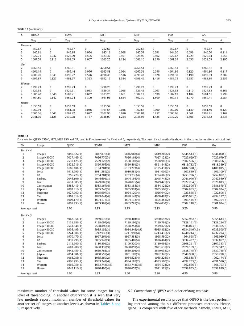
Table 14Data sets for QIPSO, TSMO, MTT, MBF, PSO and GA, used in Friedman test for K = 4 and 5, respectively. The rank of each method is shown in the parentheses after statistical test.

SN Image QIPSO TSMO MTT MBF PSO GA

For K = 41 Image1 5850.622(1) 5847.876(3) 5846.982(4) 5849.289(2) 5845.543(5) 5844.000(6)2 ImageN30C30 7027.449(1) 7026.770(3) 7026.163(4) 7027.123(2) 7025.629(6) 7025.679(5)3 ImageN30C80 7510.425(1) 7509.129(2) 7508.101(4) 7508.986(3) 7507.566(5) 7506.266(6)4 ImageN80C30 6822.516(1) 6820.365(4) 6820.461(3) 6821.443(2) 6819.732(5) 6818.339(6)5 ImageN80C80 6186.481(1) 6184.204(3) 6183.273(4) 6185.431(2) 6182.320(5) 6180.015(6)6 Lena 1913.793(1) 1911.289(2) 1910.581(4) 1911.009(3) 1907.880(5) 1906.109(6)7 B2 3756.729(1) 3754.204(3) 3753.736(4) 3754.866(2) 3753.736(5) 3752.882(6)8 Barbara 2046.106(1) 2044.691(3) 2044.156(4) 2045.745(2) 2041.976(6) 2042.560(5)9 Boat 2631.609(1) 2629.086(3) 2628.075(4) 2629.425(2) 2627.264(5) 2626.013(6)

10 Cameraman 3585.419(1) 3583.167(4) 3583.185(3) 3584.124(2) 3582.596(5) 3581.875(6)11 Jetplane 2007.816(1) 2005.240(3) 2005.993(4) 2005.506(2) 2004.863(6) 2004.924(5)12 Pinecone 1027.767(1) 1025.907(3) 1024.120(4) 1026.640(2) 1023.858(5) 1022.806(6)13 Car 4901.312(1) 4899.044(4) 4898.142(3) 4900.499(2) 4895.981(5) 4894.197(6)14 Woman 1606.179(1) 1604.177(3) 1604.132(4) 1605.381(2) 1603.435(5) 1602.394(6)15 House 2005.433(1) 2003.397(4) 2003.285(3) 2004.030(2) 2002.218(5) 2001.624(6)

Average rank 1.00 3.13 3.73 2.13 5.20 5.80

For K = 51 Image1 5962.951(1) 5959.670(3) 5958.404(4) 5960.642(2) 5957.982(5) 5955.644(6)2 ImageN30C30 7131.386(1) 7129.097(4) 7129.196(3) 7129.791(2) 7128.161(6) 7128.224(5)3 ImageN30C80 7541.848(1) 7538.890(3) 7538.253(4) 7539.879(2) 7536.023(5) 7534.305(6)4 ImageN80C30 6936.493(1) 6935.152(3) 6934.546(4.5) 6935.852(2) 6934.546(4.5) 6933.595(6)5 ImageN80C80 6244.686(1) 6242.936(3) 6241.998(4) 6243.436(2) 6240.214(5) 6237.274(6)6 Lena 1970.475(1) 1967.264(4) 1967.388(3) 1968.580(2) 1964.868(5) 1963.080(6)7 B2 3839.299(1) 3835.943(3) 3835.405(4) 3836.464(2) 3834.437(5) 3832.857(6)8 Barbara 2112.660(1) 2110.801(2) 2109.320(4) 2110.694(3) 2108.221(5) 2107.333(6)9 Boat 2683.900(1) 2680.339(3) 2680.059(4) 2681.635(2) 2678.109(5) 2677.347(6)

10 Cameraman 3642.459(1) 3639.763(3) 3639.304(4) 3640.038(2) 3638.745(5) 3637.765(6)11 Jetplane 2054.581(1) 2050.559(4) 2051.189(3) 2052.320(2) 2049.960(6) 2050.298(5)12 Pinecone 1068.083(1) 1065.369(2) 1064.528(4) 1065.226(3) 1063.588(5) 1062.174(6)13 Car 4996.493(1) 4993.242(4) 4994.185(2) 4993.500(3) 4992.253(5) 4991.586(6)14 Woman 1666.051(1) 1663.744(3.5) 1663.744(3.5) 1664.123(2) 1662.866(5) 1661.793(6)15 House 2042.110(1) 2040.490(4) 2040.652(3) 2041.571(2) 2039.855(5) 2038.839(6)

Average rank 1.00 3.23 3.60 2.20 4.90 5.86

Table 13 (continued)



Pinecone2 752.67 0 752.67 0 752.67 0 752.67 0 752.67 0 752.67 03 945.81 0 945.18 0.054 945.19 0.068 945.57 0.091 944.20 0.099 940.50 0.1144 1027.71 0.042 1025.09 0.595 1023.37 0.491 1025.95 0.502 1022.67 1.229 1020.64 1.2535 1067.59 0.113 1063.63 1.067 1063.25 1.124 1063.16 1.250 1061.39 2.036 1059.58 2.195

Car2 4260.51 0 4260.51 0 4260.51 0 4260.51 0 4260.51 0 4260.51 03 4666.19 0 4665.44 0.056 4665.88 0.064 4665.51 0.086 4664.86 0.120 4664.86 0.1174 4900.70 0.043 4898.27 0.576 4898.43 0.516 4899.43 0.628 4894.30 2.190 4892.93 2.3825 4995.87 0.127 4991.67 1.323 4992.17 1.534 4991.49 1.416 4989.75 2.387 4988.89 2.255

Woman2 1298.23 0 1298.23 0 1298.23 0 1298.23 0 1298.23 0 1298.23 03 1529.55 0 1529.31 0.053 1529.34 0.065 1529.45 0.063 1528.52 0.110 1527.83 0.1664 1605.40 0.046 1603.21 0.637 1603.20 0.661 1604.12 0.599 1602.19 1.184 1601.51 1.2985 1664.89 0.142 1662.24 1.300 1661.93 1.624 1662.39 1.509 1660.11 1.970 1659.41 2.284

House2 1653.59 0 1653.59 0 1653.59 0 1653.59 0 1653.59 0 1653.59 03 1962.94 0 1961.98 0.046 1961.54 0.086 1962.87 0.060 1962.00 0.130 1961.50 0.1294 2005.36 0.043 2002.92 0.677 2002.96 0.686 2003.02 0.757 2000.66 1.061 1999.91 1.1625 2041.39 0.125 2039.08 1.167 2038.99 1.254 2038.95 1.425 2037.20 2.506 2036.52 2.536


maximum number of threshold values for some images for anylevel of thresholding. In another observation it is seen that veryfew methods report maximum number of threshold values foranother set of images at another levels as shown in Tables 8 and9, respectively.

6.2. Comparison of QIPSO with other existing methods

The experimental results prove that QIPSO is the best perform-ing method among the six different proposed methods. Hence,QIPSO is compared with five other methods namely, TSMO, MTT,

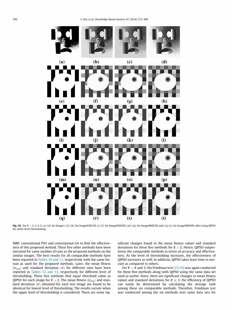
Fig. 10. For K ¼ 2;3;4;5, (a)–(d), for Image1, (e)–(h), for ImageN30C30, (i)–(l), for ImageN30C80, (m)–(p), for ImageN80C30, and, (q)–(t), for ImageN80C80, after using QIPSOfor multi-level thresholding.


MBF, conventional PSO and conventional GA to find the effective-ness of this proposed method. These five other methods have beenexecuted for same number of runs as the proposed methods on thesimilar images. The best results for all comparable methods havebeen reported in Tables 10 and 11, respectively with the same for-mat as used for the proposed methods. Later, the mean fitnessðUavgÞ and standard deviation ðrÞ for different runs have beenreported in Tables 12 and 13, respectively for different level ofthresholding. These five methods find equal threshold value asQIPSO for each image for K ¼ 2. The mean fitness ðUavgÞ and stan-dard deviation ðrÞ obtained for each test image are found to beidentical for lowest level of thresholding. The results variate whenthe upper level of thresholding is considered. There are some sig-

nificant changes found in the mean fitness values and standarddeviations for these five methods for K > 2. Hence, QIPSO outper-forms the comparable methods in terms of accuracy and effective-ness. As the level of thresholding increases, the effectiveness ofQIPSO increases as well. In addition, QIPSO takes least time to exe-cute as compared to others.

For K ¼ 4 and 5, the Friedman test [15,16] was again conductedfor these five methods along with QIPSO using the same data setused as earlier. Since, there are significant changes in mean fitnessvalues and standard deviations for K P 3, the efficiency of QIPSOcan easily be determined by calculating the average rankamong these six comparable methods. Therefore, Friedman testwas conducted among the six methods over same data sets for

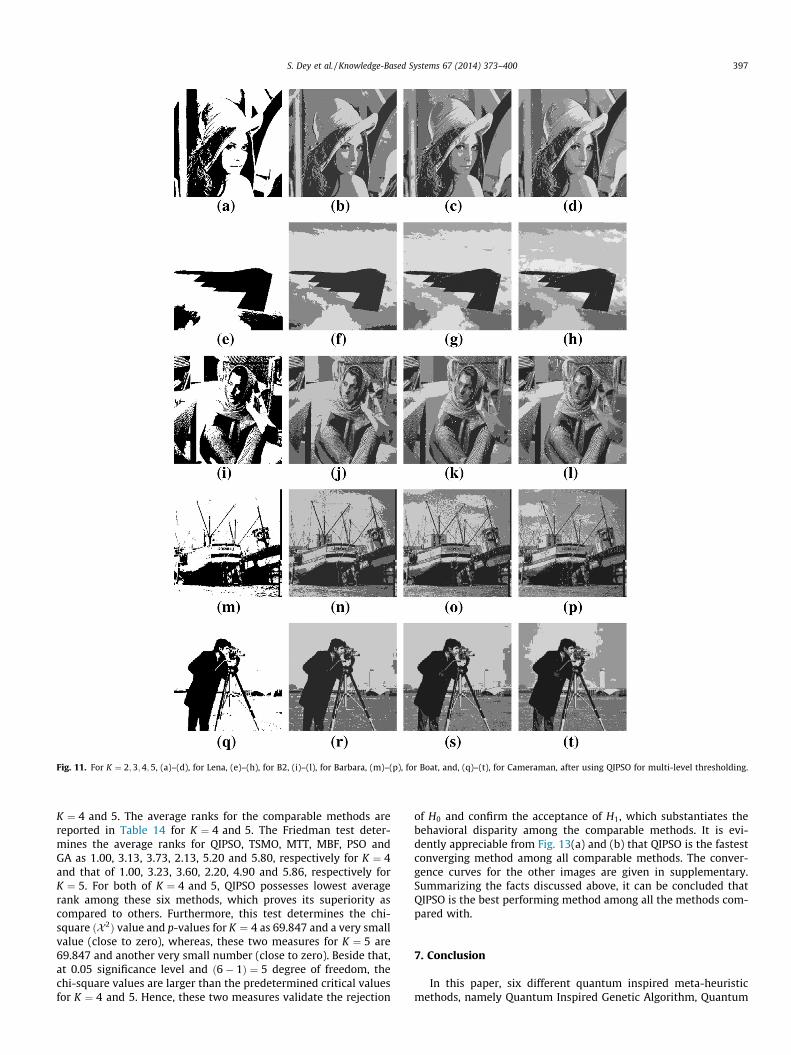
Fig. 11. For K ¼ 2;3;4;5, (a)–(d), for Lena, (e)–(h), for B2, (i)–(l), for Barbara, (m)–(p), for Boat, and, (q)–(t), for Cameraman, after using QIPSO for multi-level thresholding.


K ¼ 4 and 5. The average ranks for the comparable methods arereported in Table 14 for K ¼ 4 and 5. The Friedman test deter-mines the average ranks for QIPSO, TSMO, MTT, MBF, PSO andGA as 1.00, 3.13, 3.73, 2.13, 5.20 and 5.80, respectively for K ¼ 4and that of 1.00, 3.23, 3.60, 2.20, 4.90 and 5.86, respectively forK ¼ 5. For both of K ¼ 4 and 5, QIPSO possesses lowest averagerank among these six methods, which proves its superiority ascompared to others. Furthermore, this test determines the chi-square ðX2Þ value and p-values for K ¼ 4 as 69.847 and a very smallvalue (close to zero), whereas, these two measures for K ¼ 5 are69.847 and another very small number (close to zero). Beside that,at 0.05 significance level and ð6� 1Þ ¼ 5 degree of freedom, thechi-square values are larger than the predetermined critical valuesfor K ¼ 4 and 5. Hence, these two measures validate the rejection

of H0 and confirm the acceptance of H1, which substantiates thebehavioral disparity among the comparable methods. It is evi-dently appreciable from Fig. 13(a) and (b) that QIPSO is the fastestconverging method among all comparable methods. The conver-gence curves for the other images are given in supplementary.Summarizing the facts discussed above, it can be concluded thatQIPSO is the best performing method among all the methods com-pared with.

7. Conclusion

In this paper, six different quantum inspired meta-heuristicmethods, namely Quantum Inspired Genetic Algorithm, Quantum

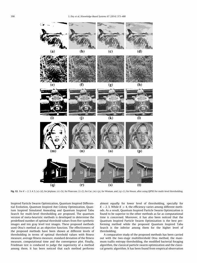
Fig. 12. For K ¼ 2;3;4;5, (a)–(d), for Jetplane, (e)–(h), for Pinecone, (i)–(l), for Car, (m)–(p), for Woman, and, (q)–(t), for House, after using QIPSO for multi-level thresholding.


Inspired Particle Swarm Optimization, Quantum Inspired Differen-tial Evolution, Quantum Inspired Ant Colony Optimization, Quan-tum Inspired Simulated Annealing and Quantum Inspired TabuSearch for multi-level thresholding are proposed. The quantumversion of meta-heuristic methods is developed to determine thepredefined number of optimal threshold values from five syntheticimages and ten gray level test images. These proposed methodsused Otsu’s method as an objective function. The effectiveness ofthe proposed methods have been shown at different levels ofthresholding in terms of optimal threshold values with fitnessmeasure, average fitness measure, standard deviation of the fitnessmeasure, computational time and the convergence plot. Finally,Friedman test is conduced to judge the superiority of a methodamong them. It has been noticed that each method performs

almost equally for lower level of thresholding, specially forK ¼ 2;3. While K P 4, the efficiency varies among different meth-ods. As a result, Quantum Inspired Particle Swarm Optimization isfound to be superior to the other methods as far as computationaltime is concerned. Moreover, it has also been noticed that theQuantum Inspired Particle Swarm Optimization is the best per-forming method while the proposed Quantum Inspired TabuSearch is the inferior among them for the higher level ofthresholding.

A comparative study of the proposed methods has been carriedout with the two-stage multithreshold Otsu method, the maxi-mum tsallis entropy thresholding, the modified bacterial foragingalgorithm, the classical particle swarm optimization and the classi-cal genetic algorithm. It has been found from empirical observation

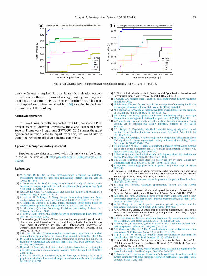
0 200 400 600 800 1000 1200 1400 1600 1800 20001900

1902

1904

1906

1908

1910

1912

1914Convergence curves for the comparable algorithms for K=4

Number of generation

Fitn

ess

valu

e (U

)

QIPSOTSMOMTTMBFPSOGA

(n) Number of generation (n)

(a)

0 200 400 600 800 1000 1200 1400 1600 1800 2000

1958

1960

1962

1964

1966

1968

1970

Fitn

ess

valu

e (U

)

Convergence curves for the comparable algorithms for K=5

QIPSOTSMOMTTMBFPSOGA

(b)

Fig. 13. Convergence curves of the comparable methods for Lena: (a) for K ¼ 4 and (b) for K ¼ 5.


that the Quantum Inspired Particle Swarm Optimization outper-forms these methods in terms of average ranking, accuracy androbustness. Apart from this, as a scope of further research, quan-tum inspired multiobjective algorithm [64] can also be designedfor multi-level thresholding.

Acknowledgements

This work was partially supported by UGC sponsored UPE-IIproject grant of Jadavpur University, India and European UnionSeventh Framework Programme (FP7/2007–2013) under the grantagreement number: 246016. Apart from this, we would like tothank the reviewers for their valuable comments.

Appendix A. Supplementary material

Supplementary data associated with this article can be found,in the online version, at http://dx.doi.org/10.1016/j.knosys.2014.04.006.

References

[1] M. Sezgin, R. Tasaltin, A new dichotomization technique to multilevelthresholding devoted to inspection applications, Pattern Recogni. Lett. 21(2000) 151–161.

[2] K. hammouche, M. Diaf, P. Siarry, A comparative study of various meta-heuristic techniques applied to the multilevel thresholding problem, Eng. Appl.Artif. Intell. 23 (2010) 678–688.

[3] P.S. Liao, T.S. Chen, P.C. Chung, A fast algorithm for multilevel thresholding, J.Inform. Sci. Eng. 17 (2001) 713–727.

[4] A. Nakiba, H. Oulhadja, P. Siarry, Image thresholding based on Paretomultiobjective optimization, Eng. Appl. Artif. Intell. 23 (3) (2010) 313–320.

[5] A. Nakiba, H. Oulhadja, P. Siarry, Image histogram thresholding based onmultiobjective optimization, Signal Process. 87 (2007) 2516–2534.

[6] D. Mcmohan, Quantum Computing Explained, John Wiley & Sons, Inc.,Hoboken, New Jersey, 2008.

[7] V. Vendral, M.B. Plenio, M.A. Rippin, Quantum entanglement, Phys. Rev. Lett.78 (12) (1997) 2275–2279.

[8] S. Bhattacharyya, S. Dey, An efficient quantum inspired genetic algorithm withchaotic map model based interference and fuzzy objective function for graylevel image thresholding, in: Proc. 2011 International Conference onComputational Intelligence and Communication Systems, Gwalior, India,2011, pp. 121–125.

[9] K.H. Han, J.H. Kim, Quantum-inspired evolutionary algorithm for a classcombinational optimization, IEEE Trans. Evol. Comput. 6 (6) (2002) 580–593.

[10] U. Maulik, S. Bandyopadhyay, I. Saha, Integrating clustering and supervisedlearning for categorical data analysis, IEEE Trans. Syst. Man Cybernet. Part-A40 (4) (2010) 664–675.

[11] U. Maulik, I. Saha, Modified differential evolution based fuzzy clustering forpixel classification in remote sensing imagery, Pattern Recognit. 42 (9) (2009)2135–2149.

[12] I. Saha, U. Maulik, S. Bandyopadhyay, D. Plewczynski, Fuzzy clustering ofphysicochemical and biochemical properties of amino acids, Amino Acids 43(2) (2012) 583–594.

[13] C. Blum, A. Roli, Metaheuristic in Combinatorial Optimization: Overview andConceptual Comparison, Technical Report, IRIDIA, 2001-13.

[14] F. Glover, G.A. Kochenberger, Handbook on Metaheuristics, Kluwer AcademicPublishers, 2003.

[15] M. Friedman, The use of ranks to avoid the assumption of normality implicit inthe analysis of variance, J. Am. Stat. Assoc. 32 (1937) 674–701.

[16] M. Friedman, A comparison of alternative tests of significance for the problemof m rankings, Ann. Math. Stat. 11 (1940) 86–92.

[17] D.Y. Huang, C.-H. Wang, Optimal multi-level thresholding using a two-stageOtsu optimization approach, Pattern Recognit. Lett. 30 (2009) 275–284.

[18] Y. Zhang, L. Wu, Optimal multi-level thresholding based on maximum Tsallisentropy via an artificial bee colony approach, Entropy 13 (4) (2011)841–859.

[19] P.D. Sathya, R. Kayalvizhi, Modified bacterial foraging algorithm basedmultilevel thresholding for image segmentation, Eng. Appl. Artif. Intell. 24(2011) 595–615.

[20] M. Maitra, A. Chatterjee, A hybrid cooperative comprehensive learning basedPSO algorithm for image segmentation using multilevel thresholding, ExpertSyst. Appl. 34 (2008) 1341–1350.

[21] K. Hammouche, M. Diaf, P. Siarry, A multilevel automatic thresholding methodbased on a genetic algorithm for a fast image segmentation, Comput. Vis.Image Understand. 109 (2008) 163–175.

[22] P. Benioff, Quantum mechanical models of Turing machines that dissipate noenergy, Phys. Rev. Lett. 48 (23) (1982) 1581–1585.

[23] L.K. Grover, Quantum computers can search rapidly by using almost anytransformation, Phys. Rev. Lett. 80 (19) (1998) 4329–4332.

[24] R. Feynman, Simulating physics with computers, Int. J. Theor. Phys. 21 (1982)467–488.

[25] F. Alfares, I.I. Esat, Quantum algorithms; how useful for engineering problems,in: Proc. of the Seventh World Conference on Integrated Design and ProcessTechnology, Austin, Texas, USA, 2003, pp. 669–673.

[26] T. Hogg, Highly structured searches with quantum computers, Phys. Rev. Lett.80 (1998) 2473–2476.

[27] T. Hogg, D.A. Portnov, Quantum optimization, Inform. Sci. 128 (2000)181–197.

[28] M.P. Moore, A. Narayanan, Quantum-Inspired Computing, Department ofComputer Science, Old Library, University of Exeter, Exeter 344, UK, 1995.

[29] K.H. Han, J.H. Kim, Quantum-inspired evolutionary algorithms with a newtermination criterion, h-epsilon gate, and twophase scheme, IEEE Trans. Evol.Comput. 8 (2004) 156–169.

[30] W.J.G. Zhang, N. Li, An improved quantum genetic algorithm and itsapplication, Lect. Notes Artif. Intell. 2639 (2003) 449–452.

[31] A. Narayanan, M. Moore, Quantum inspired genetic algorithm, in: Proc. of the1996 IEEE Conference on Evolutionary Computation (ICEC ’96), NayoyaUniversity, Japan, 1996, pp. 61–66.

[32] B. Li, Z.Q. Zhuang, Genetic algorithm based-on the quantum probabilityrepresentation, Lect. Notes Comput. Sci. 2412 (2002) 500–505.

[33] A. Narayanan, T. Manneer, Quantum artificial neural network architecturesand components, Inform. Sci. 128 (2000) 231–255.

[34] G.X. Zhang, W.D.J.N. Li, L.Z. Hu, A novel quantum genetic algorithm and itsapplication, ACTA Electron. Sinica 32 (3) (2004) 476–479.

[35] L. Jiao, J. Liu, W. Zhong, An organizational coevolutionary algorithm forclassification, IEEE Trans. Evol. Comput. 10 (1) (2006) 67–80.

[36] K. Kennedy, R. Eberhart, Particle swarm optimization, in: Proceedings of theIEEE International Conference on Neural Networks (ICNN95), Perth, Australia,vol. 4, 1995, pp. 1942–1948.

[37] T. Sousa, A. Silva, A. Neves, Particle swarm based data mining algorithms forclassification tasks, Parallel Comput. 30 (2004) 267–783.

[38] A. Ratnaweera, S. Halgamuge, H. Watson, Self-organizing hierarchical particleswarm optimizer with time-varying acceleration coefficients, IEEE Trans. Evol.Comput. 8 (2004) 240–255.



http://refhub.elsevier.com/S0950-7051(14)00128-2/h0080














































































[39] P. Angeline, Using selection to improve particle swarm optimization, in: Proc.of the IEEE Congress on Evolutionary Computation, Anchorage, AK, 1998, pp.84–89.

[40] R. Brits, A. Engelbrecht, F. van den Bergh, A niching particle swarm optimizer,in: Proc. of the 4th Asia-Pacific Conference on Simulated EvolutionaryLearning, Singapore, 2002, pp. 692–696.

[41] D. Parrott, X. Li, Locating and tracking multiple dynamic optima by a particleswarm model using speciation, IEEE Trans. Evol. Comput. 10 (2006) 440–458.

[42] R. Parpinelli, H. Lopes, A. Freitas, Data mining with an ant colony optimizationalgorithm, IEEE Trans. Evol. Comput. 6 (4) (2002) 321–332.

[43] J.S.M. Schreiber, T. Vojta, Interacting electrons in parabolic quantum dots:energy levels, addition energies, and charge distributions, Int. J. Modern Phys.B 15 (2001) 3641.

[44] G. Pampara, A. Engelbrecht, N. Franken, Binary differential evolution, in: Proc.of the IEEE Congress on Evolutionary Computation, 2006, pp. 1873–1879.

[45] S. Fengjie, W. He, F. Jieqing, 2d Otsu segmentation algorithm based onsimulated annealing genetic algorithm for iced-cable images, in: Proc. ofInternational Forum on Information Technology and Applications (IFITA 2009),Chengdu, China, vol. 2, 2009, pp. 600–602.

[46] W. Luo, W. Wang, H. Liao, Image segmentation on colonies images by acombined algorithm of simulated annealing and genetic algorithm, in: Proc. ofFourth International Conference on Image and Graphics (ICIG 2007), Chengdu,China, 2007, pp. 342–346.

[47] L. Tang, K. Wang, G. Feng, Y. Li, An image segmentation algorithm based on thesimulated annealing and improved snake model, in: Proc. of InternationalConference on Mechatronics and Automation (ICMA 2007), Harbin,Heilongjiang, China, 2007, pp. 3876–3881.

[48] A. Nakib, H. Oulhadj, P. Siarry, Non-supervised image segmentation based onmultiobjective optimization, Pattern Recognit. Lett. 29 (2) (2008) 161–172.

[49] C. Yufei, Z. Weidong, W. Zhicheng, Level set segmentation algorithm based onimage entropy and simulated annealing, in: Proc. of 1st InternationalConference on Bioinformatics and Biomedical Engineering (ICBBE 2007),China, 2007, pp. 999–1003.

[50] G. Garrido, S. Furuie, A. Orgambide, Refinement of left ventricle segmentationin mri based on simulated annealing, in: Proc. of the 20th Annual InternationalConference of the IEEE Engineering in Medicine and Biology Society, HongKong Sar, China, vol. 20, issue 2, 1998, pp. 598–601.

[51] F. Glover, M. Laguna, Tabu Search, Kluwer, Boston, MA, 1997.[52] F. Glover, Tabu search, part I, ORSA J. Comput. 1 (1989) 190–206.[53] F. Glover, Tabu search, part II, ORSA J. Comput. 2 (1990) 4–32.[54] U. Faigle, W. Kern, Some convergence results for probabilistic tabu search,

ORSA J. Comput. 4 (1992) 32–37.[55] B. Fox, Integrating and accelerating tabu search, simulated annealing and

genetic algorithms, Ann. Oper. Res. 41 (1993) 47–67.[56] M. Sezgin, B. Sankur, Survey over image thresholding techniques and

quantitative performance evaluation, J. Electron. Imaging 13 (1) (2004) 146–165.

[57] N. Otsu, A threshold selection method from gray level histograms, IEEE Trans.Syst. Man Cybernet. 9 (1979) 62–66.

[58] R. Storn, K. Price, Differential Evolution – A Simple and Efficient Heuristic forGlobal Optimization over Continuous Spaces, Technical Report TR-95-012,ICSI.

[59] Z.B. Zabinsky, Stochastic Adaptive Search for Global Optimization, Springer,Berlin, 2003.

[60] A. Zhigljavsky, Stochastic Global Optimization, Springer, Berlin, 2008.[61] S. Paterlini, T. Krink, Differential evolution and particle swarm optimisation in

partitional clustering, Comput. Stat. Data Anal. 50 (2006) 1220–1247.[62] M. Dorigo, V. Maniezzo, A. Colorni, The ant system: optimization by a colony of

cooperating agents, IEEE Trans. Syst. Man Cybernet. – Part B 26 (1) (1996) 29–41.

[63] S. Kirkpatrik, C.D. Gelatt, M.P. Vecchi, Optimization by simulated annealing,Science 220 (1983) 671–680.

[64] I. Saha, U. Maulik, D. Plewczynski, A new multi-objective technique fordifferential fuzzy clustering, Appl. Soft Comput. 11 (2) (2011) 2765–2776.





































Documents

Multi-level thresholding using quantum inspired meta ... · PDF fileMulti-level thresholding using quantum inspired meta-heuristics ... Ant Colony Optimization, Quantum Inspired Simulated