Multi-items Batch Scheduling Model for a Batch Processor

73

Jurnal Teknik Industri, Vol. 20, No. 1, June 2018, 73-88 DOI: 10.9744/jti.20.1.73-88

ISSN 1411-2485 print / ISSN 2087-7439 online

Multi-items Batch Scheduling Model for a Batch Processor to Minimize Total Actual Flowtime of Parts through the Shop

Nita PA Hidayat1*, Andi Cakravastia2, TMA Ari Samadhi2 and Abdul Hakim Halim2

Abstract: This study is inspired by a batch scheduling problem in metal working industry which

guarantees to satisfy a due date. The actual flowtime adopts the backward scheduling approach and considers the due date. Using the actual flowtime as the objective, means that the solution is oriented to satisfy the due date, and simultaneosly to minimize the length of time of the parts spending in the shop. This research is to address a problem of scheduling batches consisting of multiple items of parts processed on a batch processor where the completed parts must be delivered several time at different due dates. We propose an algorithm maximize the utilization of the batch processor and to schedule the resulting batches in backwardly non increasing batch size. Keywords: Backward scheduling; batch scheduling; batch processor; batch size; actual flowtime.

Introduction

A number of parts processed simultaneously with

sharing a setup time could be defined as a batch, and

a batch processor is a machine that processes one

batch at a time. Today the batch processor is encoun-

tered in many different environments, such as burn-

in operations in semiconductor industry (Cheng, et

al. [1]), heating and pressure operations in aeronau-

tical industry (Malapert, et al. [2]), hardening and

soaking operations in automobile gear manufac-

turing (Gokhalea and Mathirajan [3]), and drying

operations in lumber industry (Gaudreault, et al.

[4]). The batch processor is also used in iron and steel

industry for heating ingots up to a proper processing

temperature (Gong, et al. [5]), microbiological labora-

tory for producing agar that is used in food testing

(Chakhlevit, et al.[6]), and bicycle rim manufacturing

(Damodaran, et al. [7]). Those pieces of research

work have addressed problems of batch scheduling

on the batch processor.

The solution for batch scheduling problems on a

batch processor is determined through two phases,

that are batching and scheduling. Decisions on the

batch size are madein the batching phase i.e., group-

ing the parts into some batches, while arranging the

resulting batches into a specific sequence is

performed in the scheduling phase. The size of a

batch represents a number of parts in the batch, and

it is limited by capacity of the batch processor.

1 Faculty of Technology, Department of Industrial Engineering,

Universitas Jendarl Achmad Yani, Jl. Terusan Gatot Subroto,

P.O BOX 807, Bandung 40285, INDONESIA.

Email: [email protected]. 2 Faculty of Industrial Technology, Department of Industrial Engi-

neering, JL. Ganesha 10, Bandung 40132, INDONESIA.

Email: [email protected]; [email protected];

[email protected].

* Corresponding author

Grouping parts in the batching phase should be

based on a certain rule. Guo, Chengtao [8] has

grouped parts based on the order of processing

machines which is required by the parts. While

Dauzère-Peres and Monch [9] and Chakhlevitch et

al. [6] have grouped parts based on the type of family

of the parts, all parts in the same batch must come

from the same type of family.

The entire parts in the same batch are processed

simultaneously during a certain period of time called

batch processing time, although each part requires a

certain processing time which may differ from

others. In Cheng et al. [1] and Condotta et al [10] the

entire parts in the batch have the same processing

time, and the processing time of batch equals the

processing time of parts. While in Noroozi, et al. [11],

Behnamian et al. [12], Khasan, et al. [13] and Parsa,

et al. [14] the processing time for each part is

different. They set the processing time of batch

equals the longest processing time of parts in the

batch because they assume that an excessive

duration of processing the parts could not lead to any

defect. On the contrary, in Bellanger, et al. [15] each

part has the processing time and a certain limit of

processing time. They allow the real processing time

of parts exceed its processing time as long as it does

not exceed its certain limit of processing time

because the excessive processing time from its limit

may cause any defects. Therefore, only parts whose

processing time intervals intersect can be formed

into a batch.

Those studies adopt the forward scheduling

approach, i.e., sequencing jobs starts from the time

zero, then moving forward to the due date until all

jobs have been scheduled. The schedule is feasible,

but there is no guarantee it could meet the due date.

On the other hand, Halim et al. [16] defined the

actual flowtime of parts as the time that the parts

mailto:[email protected]

Hidayat et al. / Multi-item Batch Scheduling Model / JTI, Vol. 20, No. 1, June 2018, pp. 73-88

74

spend in the shop from the starting time of

processing until their due date as the delivery time

of the processed parts, and the actual flowtime

adopts a backward scheduling approach i.e.,

sequencing jobs starts from the due date then

moving backward to the time zero until all jobs have

been scheduled. The backward scheduling approach

can satisfy the due date, but it may lead to an

infeasible schedule. This research is inspired by a

batch scheduling problem in metal working industry

which guarantees to satisfy the due date as a

commitment to its customer, thus adopting

backward scheduling approach is a must. It is

assumed that the resulted schedule is always

feasible, and the infeasible schedule case will be

discussed in future research.

The actual flowtime has been applied to problems of

batch scheduling by Halim et al. [17, 18, 19], Sukoyo

et al. [20] and Zahedi et al. [21] but they conduct

batch scheduling research for job processors i.e., the

machine that processes one job at a time. Hidayat et

al. [22, 23] develop the actual flowtime of parts for

batch scheduling problems on batch processors, and

adopt it as an objective where parts to be processed

are a single item with a common due date. Those

model is further developed by Hidayat et al. [24] into

a condition where the parts should be delivered at

different due dates. Halim et al. [25] also develop the

actual flowtime of parts for batch scheduling

problems on batch processors into a condition where

a batch could have different set up time from those of

the other batches.

This research is concerned on batch scheduling

problems at the coating stage performed on a batch

processor in metal working industry. The length of

time for the coating process is determined by coating

thickness of part. When the parts are processed less

or more than the time required for coating, then the

part will not in accordance with the product

specifications. Therefore, only parts which have the

same processing time can be grouped into the same

batch. We define that the parts which have the same

requirement of coating thickness are compatible and

have the same type of item. Therefore, grouping

parts into batches should be based on the same type

of item. The metal working industry produces some

different products and demanded at different due

dates. Each part requires a certain coating thickness

depending on the product that will be formed by the

parts, so that at the coating stage, there are some

parts require different thickness and demanded at

different due dates. Accordingly, we need to develop

the model in Hidayat, et al. [24] into a condition of

multiple items of parts with multiple due dates

(abbreviated as MIMD). The model is developed in

two steps; the first step is that the single item is

developed into multiple items of parts with a com-

mon due date, and at the second step the developed

model is further developed into multiple items of

parts with multiple due dates.

Methods

The MIMD problem can be explained as follows. Let

there be numbers, of multiple items

parts demanded at due dates,

respectively. The parts must be processed on a batch

processor, and is the part processing time of item

g. The batch processor needs to be set up before

processing a batch, the set up times depends on the

item type of parts in the batch, and is the set up

time for item g. The set up time is independent to the

sizes of batches and the position of batches in the

shop. The problems are both to determine batch size

of the multiple items parts and to sequence the

formed batches so as to minimize the total actual

flowtime of parts through the shop ( ).

The following the symbols and notations are used in

this paper.

Indexes : part item, g =1, 2, ..., k : time interval in a scheduling period, h = 1, 2,

..., r. It is counted from the end position on a

time scale. : position of a batch on a production schedule

which is counted from the end position on a

time scale.

Sets : set of parts in a batch sequenced at position i

(i = 1, 2, ..., N) : set of parts in a batch sequenced at position i

(i =1, 2, ..., ) within interval

Parameters : capacity of batch processor : common due date : the due date : time period defined as:

for ( ) for

: number of item types : number of machine : number of parts item g demanded at com-

mon due date : total part demanded at common due date,

∑

: number of parts item g demanded at due

date

: number of parts demanded at due date ,

∑

: number of intervals in the whole scheduling

period


75

: setup time of batch sequenced at position i : setup time of batch sequenced at position

within interval : setup time of item

: processing time of batch sequenced at posi-

tion i : processing time of batch sequenced at posi-

tion within interval : part processing time of item g

Variables : starting time of processing batch sequenced

at position i : starting time of processing batch sequenced

at position within interval : number of parts processed within interval

: total actual flowtime of parts through the

shop : type of item part in the batch sequenced at

position i : number of shortage parts within interval

: number of batches which consisting of part

item

: number of batches in the whole scheduling

period : number of batches which consisting of part

item within interval

: number of batches within interval ,

∑

: number of parts in batch sequenced at posi-

tion i : number of parts in batch sequenced at posi-

tion within interval

: number of parts item requested to be pro-

cessed within interval : binary variable equals 1 if parts in the batch

sequenced at position i are members of item

, otherwise 0

: binary variable equals 1 if parts in the batch

sequenced at position within interval

are members of item , otherwise 0

Actual Flowtime as a Performance

Measurement

The actual flowtime of parts is defined as the time

required by parts to be on a shop. It is measured

from the processing starting times to their due date

or to their delivery time (Halim, et al. [16]). In an

ideal condition, the part spends in the shop when it

is processed. So that the part’s actual flowtime

equals to the part procesing time. It can be happened

if the part arrives exactly at its processing starting

time and delivers right after completing the process.

It is assumed that the arrival of parts as a batch can

be setup exactly at its processing starting time. The

actual flowtime of parts will be higher than its

processsing time if those parts are completed before

their due date. In this case, the parts require longer

time on the shop, since they have to wait until they

deliver to the customer at the due date. Therefore,

minimizing the actual flowtime of parts is essentially

minimizing the waiting time before the delivery time

(due date). Hence, the time duration spends by those

parts in the shop is minimized.

Using the definition in Halim, et al. [16],

denotes the actual flowtime of part in batch ,

and is part in batch , then the actual

flowtime of part is as follows.

(1)

The actual flowtime of batch (denoted by )

states the length of time the batch spends on the

shop from its arrival time until its due date (see.

equation (2))

(2)

A concept of the actual flowtime for parts of single

item demanded on a common due date have been

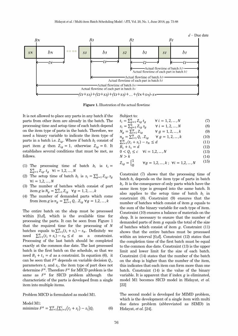
developed in Hidayat, et al. [22]. Figure 1 shows the

sequence of the N batches processed on a single

batch processor. is determined in equation (3),

and the total actual flowtime of batches through the

shop (expressed by ) is determined in equation

(4).

{∑ ( )

} (3)

∑ {∑ ( ) }

(4)

The actual flowtime of each part in the same batch

equals the actual flowtime of batch, and total actual

flowtime of parts in a batch is a multiplication of the

actual flowtime of the batch by the number of parts

in the batch. The total actual flowtime of parts

through the shop for a single item with a common

due date on a batch processor is determined in

equation (5).

∑ {∑ ( ) }

(5)

Model Development

The first model was developed for multiple items of

parts with a common due date problem (MICD). The

MICD is a development of a single item with

common due date problem (abbreviated as SICD) in

Hidayat, et al. [22]. The difference between those two

lies in the number of item type of parts, while

simultaneously on a common due date. Under the

condition of multiple items, the processed part

consist of several different items and each item has

different processing time and set up time.


76

It is not allowed to place any parts in any batch if the

parts from other item are already in the batch. The

processing time and setup time of each batch depend

on the item type of parts in the batch. Therefore, we

need a binary variable to indicate the item type of

parts in a batch i.e. . Where if batch consist of

part item g then , otherwise . It

establishes several conditions that must be met, as

follows.

(1) The processing time of batch is ∑

(2) The setup time of batch is ∑

(3) The number of batches which consist of part

item g is ∑

(4) The number of demanded parts which come

from item g is ∑

The entire batch on the shop must be processed

within [0,d], which is the available time for

processing the parts. It can be seen from Figure 1

that the required time for the processing of

batches equals to ∑ ( ) . Definitely we

need ∑ ( ) as a constraint.

Processing of the last batch should be completed

exactly at the common due date. The last processed

batch is the first batch on the schedule, so that we

need as a constraint. In equation (6), it

can be seen that depends on variable decision parameters and , the item type of part does not

determine . Therefore for MICD problem is the

same as for SICD problem although the

characteristic of the parts is developed from a single

item into multiple items.

Problem MICD is formulated as model M1.

Model M1:

∑ {∑ ( ) }

(6)

Subject to:

∑ (7)

∑ (8)

∑ (9)

∑ (10)

∑ ( ) (11)

(12) (13) (14)

{ (15)

Constraint (7) shows that the processing time of

batch depends on the item type of parts in batch

. It is the consequence of only parts which have the

same item type is grouped into the same batch. It

also applies to the setup time of batch in

constraint (8). Constraint (9) ensures that the

number of batches which consist of item equals to

the sum of the binary variable for each type of item.

Constraint (10) ensures a balance of materials on the

shop. It is necessary to ensure that the number of

demanded parts of item equals the total of the size

of batches which consist of item . Constraint (11)

shows that the entire batches must be processed

within an interval [0,d]. Constraint (12) states that

the completion time of the first batch must be equal

to the common due date. Constraint (13) is the upper

limit and lower limit for the size of each batch.

Constraint (14) states that the number of the batch

on the shop is higher than the number of the item,

this indicates that each item can form more than one

batch. Constraint (14) is the value of the binary

variable. It is apparent that if index is eliminated,

model M1 becomes SICD model in Hidayat, et al.

[22]

The second model is developed for MIMD problem,

which is the development of a single item with multi

due dates problem (abbreviated as SIMD) in

Hidayat, et al. [24].

Figure 1. Illustration of the actual flowtime


77

The difference between those two lies in the number

of item type of parts, while the similarity lies in the

parts that should be delivered several times at

different due dates. Under condition of multi due

dates, the scheduling period is divided into r

partitions of interval (h=1,2,…,r) which is the

interval between two consecutive due dates. Under

the condition of multiple items of parts, there are

demanded parts in interval which consist of

parts of item 1, parts of item 2 and parts of

item k. Therefore a binary variable i.e. is needed

This variabel indicates the item type of parts in a

batch , where if batch consists of item g then

, otherwise . It establishes several

conditions that must be met, as follow.

(1) The processing time of batch is ∑

(2) The set up time of batch is ∑

(3) The number of batches which consist of part

item g is ∑

The number of demanded parts item is

∑ and ∑

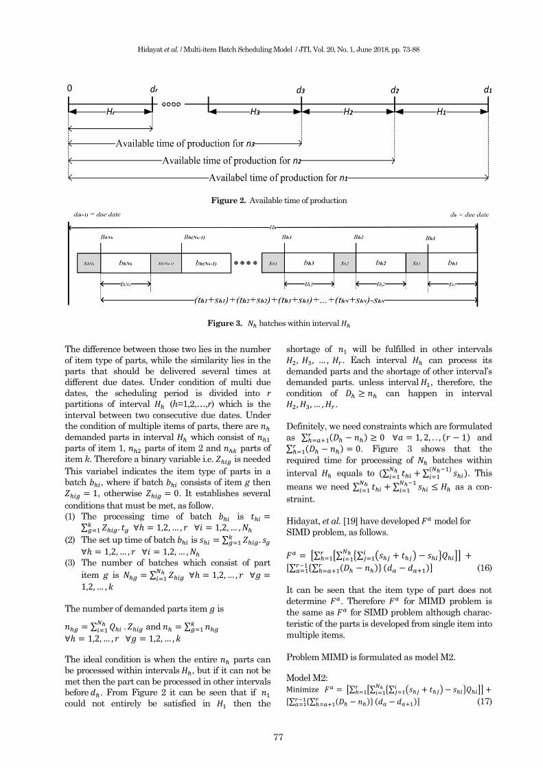
The ideal condition is when the entire parts can

be processed within intervals , but if it can not be

met then the part can be processed in other intervals

before . From Figure 2 it can be seen that if

could not entirely be satisfied in then the

shortage of will be fulfilled in other intervals

. Each interval can process its

demanded parts and the shortage of other interval’s

demanded parts. unless interval , therefore, the

condition of can happen in interval

.

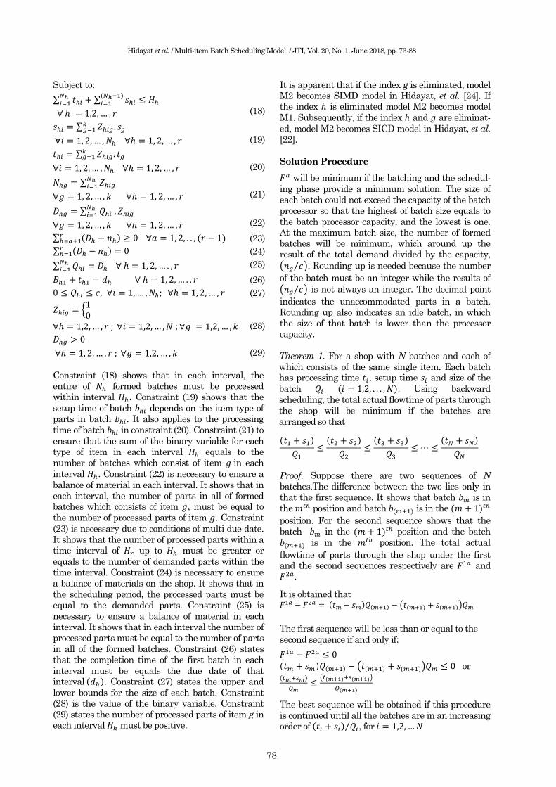
Definitely, we need constraints which are formulated

as ∑ ( ) ( ) and

∑ ( ) . Figure 3 shows that the

required time for processing of batches within

interval equals to (∑ ∑ )

( ) . This

means we need ∑ ∑

as a con-

straint.

Hidayat, et al. [19] have developed model for

SIMD problem, as follows.

[∑ [∑ {∑ ( ) }

]

]

,∑ *∑ ( ) +

( )- (16)

It can be seen that the item type of part does not

determine . Therefore for MIMD problem is

the same as for SIMD problem although charac-

teristic of the parts is developed from single item into

multiple items.

Problem MIMD is formulated as model M2.

Model M2:

[∑ [∑ {∑ ( ) }

]

]

,∑ *∑ ( ) +

( )- (17)

Figure 2. Available time of production

Figure 3. 𝑁 batches within interval 𝐻


78

Subject to:

∑ ∑

( )

(18)

∑

(19)

∑

(20)

∑

(21)

∑

(22)

∑ ( ) ( ) (23)

∑ ( ) (24)

∑ (25)

(26)

(27)

{

(28)

(29)

Constraint (18) shows that in each interval, the entire of formed batches must be processed

within interval . Constraint (19) shows that the

setup time of batch depends on the item type of parts in batch . It also applies to the processing

time of batch in constraint (20). Constraint (21) to

ensure that the sum of the binary variable for each type of item in each interval equals to the

number of batches which consist of item in each

interval . Constraint (22) is necessary to ensure a

balance of material in each interval. It shows that in each interval, the number of parts in all of formed batches which consists of item , must be equal to

the number of processed parts of item . Constraint

(23) is necessary due to conditions of multi due date. It shows that the number of processed parts within a time interval of up to must be greater or

equals to the number of demanded parts within the time interval. Constraint (24) is necessary to ensure a balance of materials on the shop. It shows that in

the scheduling period, the processed parts must be equal to the demanded parts. Constraint (25) is necessary to ensure a balance of material in each

interval. It shows that in each interval the number of processed parts must be equal to the number of parts in all of the formed batches. Constraint (26) states that the completion time of the first batch in each

interval must be equals the due date of that interval ( ). Constraint (27) states the upper and

lower bounds for the size of each batch. Constraint (28) is the value of the binary variable. Constraint (29) states the number of processed parts of item g in each interval must be positive.

It is apparent that if the index g is eliminated, model

M2 becomes SIMD model in Hidayat, et al. [24]. If the index is eliminated model M2 becomes model

M1. Subsequently, if the index and are eliminat-

ed, model M2 becomes SICD model in Hidayat, et al. [22].

Solution Procedure

will be minimum if the batching and the schedul-

ing phase provide a minimum solution. The size of each batch could not exceed the capacity of the batch processor so that the highest of batch size equals to

the batch processor capacity, and the lowest is one. At the maximum batch size, the number of formed batches will be minimum, which around up the result of the total demand divided by the capacity,

( ⁄ ). Rounding up is needed because the number

of the batch must be an integer while the results of

( ⁄ ) is not always an integer. The decimal point

indicates the unaccommodated parts in a batch. Rounding up also indicates an idle batch, in which the size of that batch is lower than the processor capacity.

Theorem 1. For a shop with N batches and each of which consists of the same single item. Each batch has processing time , setup time and size of the

batch ( ). Using backward

scheduling, the total actual flowtime of parts through the shop will be minimum if the batches are

arranged so that

( )

( )

( )

( )

Proof. Suppose there are two sequences of N batches.The difference between the two lies only in that the first sequence. It shows that batch is in

the position and batch ( ) is in the ( )

position. For the second sequence shows that the batch in the ( ) position and the batch

( ) is in the position. The total actual

flowtime of parts through the shop under the first and the second sequences respectively are and

.

It is obtained that ( ) ( ) ( ( ) ( ))

The first sequence will be less than or equal to the

second sequence if and only if:

( ) ( ) ( ( ) ( )) or ( )

( ( ) ( ))

( )

The best sequence will be obtained if this procedure is continued until all the batches are in an increasing order of ( ) ⁄ , for


79

There are N generated batches, that will be

scheduled on a batch processor. First, arrange the N

batches in any order, so that a sequence of batch

for i = 1, 2, ..., N is obtained. Next, sort the sequence

of batches increasingly in ( ) , for i = 1, 2, ...,

N (see Theorem 1).

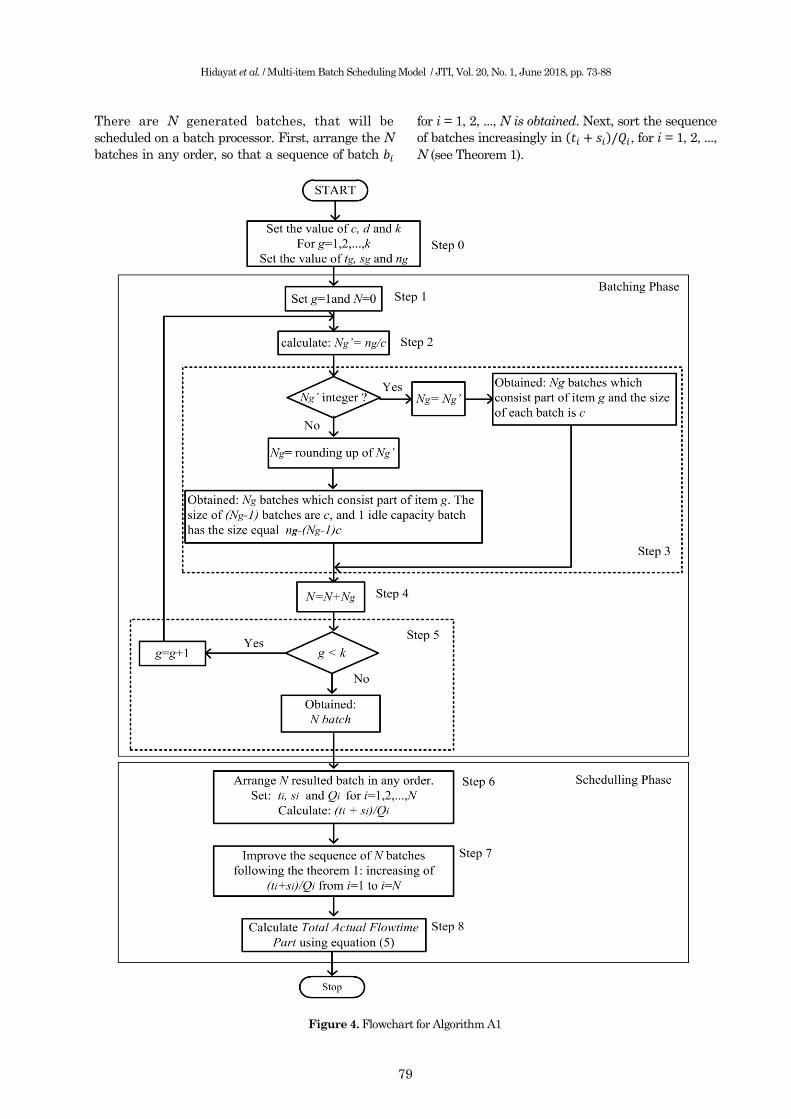
Figure 4. Flowchart for Algorithm A1


80


81

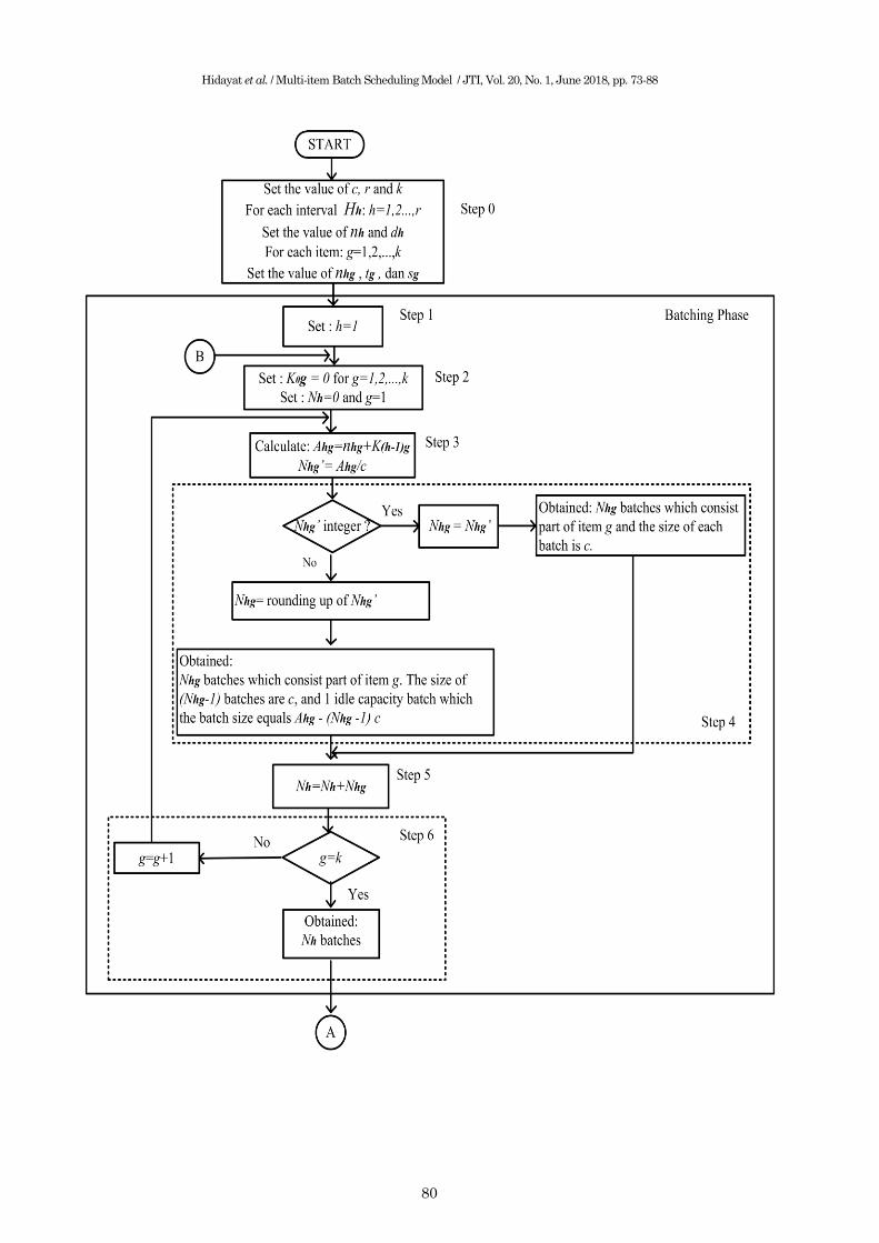
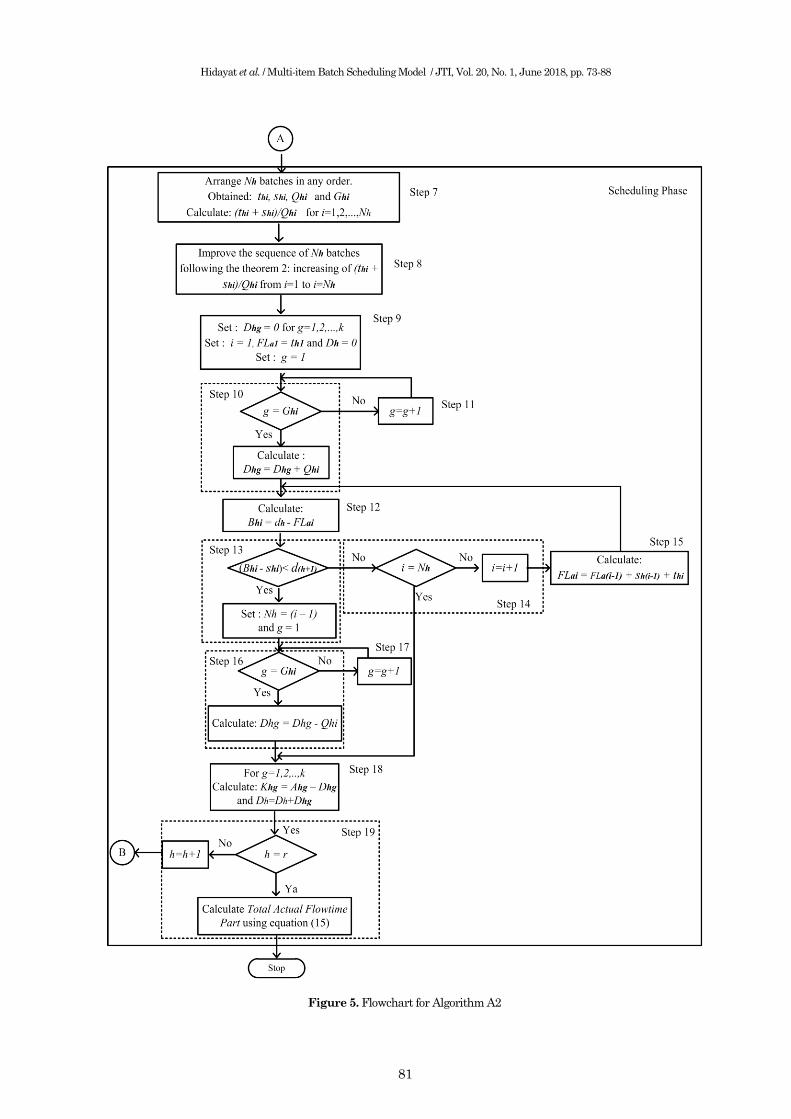
Figure 5. Flowchart for Algorithm A2


82

Algorithm A1 to solve problem MICD is developed,

and it is presented as a flowchart in Figure 4.

Algorithm A1

Step 0. Set the value of , , and

Set the value of , and ,

for .

Step 1. Set and N=0, proceed to Step 2

Step 2. Calculate

, proceed to Step 3

Step 3. If integer then and proceed to Step

4 (obtained batches which consist part of item

g and the size of each batch is );

Otherwise = rounding up of and proceed

to Step 4 (obtained batches which consist part

of item g.

The size of ( -1) batches is , and one idle

capacity batch which the batch size equals

( ) ).

Step 4. Set , proceed to Step 5

Step 5. If g k then g = g+1 and proceed to Step 2;

otherwise proceed to Step 6 (Obtained N batches)

Step 6. Arrange N resulted batches in any order, set

and for . Calculate ( ) ⁄ and proceed to Step 7

Step 7. Improve the sequence of N batches with folowing

the Theorem 1: ( )

( )

( )

( )

and proceed to Step 8.

Step 8. Calculate using equation (6) and then stop.

From Figure 2, it can be seen that under the con-

dition of multi due dates, the demanded parts ( )

can be fulfilled in some intervals before its due date

( ) unless . Definitely in each interval we need

to distinguish between the demanded part ( ), the

processed parts ( ), and the required part to

process ( ) for . The difference bet-

ween the required parts to process and the processed

parts is the shortage of parts in interval , i.e,

. Then for the next interval ( )

the required parts to process is equal to the sum of

demanded parts and the shortage of parts in the

previous interval, i.e., ( ) ( ) , and

the resulting batches ( ( ) ) is equal to the round

up of ( ) ⁄ .

Theorem 2. For a shop with r intervals (h=1,2,...,r)

and each interval has batches, each bathces

consists of the same single item. Each batch has

processing time , set up time and size of batch

(i=1,2,..., ). Using backward scheduling, the

total actual flowtime of parts through the shop will

be minimum if the batches in each interval are

arranged so that

( )

( )

( )

.

/

Proof. Suppose in the interval there are two

sequences of batches. The difference between the

two lies only in that the first sequence shows that

batch is in the position and batch ( ) is in

the ( ) position, while the second sequence

shows that the batch in the ( ) position

and the batch ( ) is in the position. The total

actual flowtime of parts through the interval under

the first and the second sequences respectively are

and

. It is obtained that

( ) ( ) ( ( )

( ))

The first sequence will be better than or equivalent

to the second sequence (

) if and only if:

( ) ( ) ( ( ) ( )) , or

( )

( ( ) ( ))

( )

The best sequence will be obtained if this procedure

is continued until all the batches are in increasing

order of ( ) ⁄ , for .

( )

( )

( )

.

/

Algorithm A2 to solve problem MIMD is developed,

and it is presented as a flowchart in Figure 5.

Algorithm A2

Step 0. Set the value of c,r dan k

Set the value of for each interval , h=1,2,...,r

Set the value of and for g=1,2,...,k

Step 1. Set h = 1 then proceed to Step 2

Step 2. Set for g=1,2,...,k;

Set and g = 1 then proceed to Step 3

Step 3. Calculate ( ) and

then proceed to Step 4

Step 4. If integer then

, and proceed to

Step 5 (obtained batches and the size of each

batch are c);

otherwise = rounding up of then proceed

to Step 5 (obtained batches which consist

part of item g.

The size of ( -1) batches are , and 1 idle capa-

city batch which the batch size equals

( ) )

Step 5. Calculate then proceed to Step 6

Step 6. If then proceed to Step 7 (obtained

batches);

otherwise then proceed to Step 3

Step 7. Arrange batches in any order (obtained

and );

Calculate: ( )

for i=1,2,..., then proceed to

Step 8

Step 8. Improve the sequence of batches with folowing

the Theorem 2, then proceed to Step 9


83

Step 9. Set for g = 1,2,..., k ;

Set i=1, , and then proceed to

Step 10 Step 10. Set g=1, then proceed to Step 11 Step 11. If then calculate , and

proceed to Step 13; otherwise proceed to Step 12

Step 12. , then proceed to Step 11 Step 13. Calculate

and proceed to Step

14 Step 14. If ( ) ( ) then and pro-

ceed to Step 17; otherwise proceed to Step 15

Step 15. If then proceed to Step 18; otherwise i = i + 1, and proceed to Step 16

Step 16. Calculate ( )

( ) , and

proceed to Step 10 Step 17. Calculate , and proceed to Step

18 Step 18. Calculate and

for , proceed to Step 19 Step 19. If then , proceed to Step 3;

otherwise calculate using equation (17), then Stop

Results and Discussions

In this section we give numerical examples for MICD and MIMD consecutively.

For the MICD case, we have the numbers of multiple items parts demanded as many as 30, 20 and 25; and the due date is 1.000 unit time. Additionally, the capacity of batch processor is 20 parts, while the processing time and the setup time of each item are presented in Table 1.

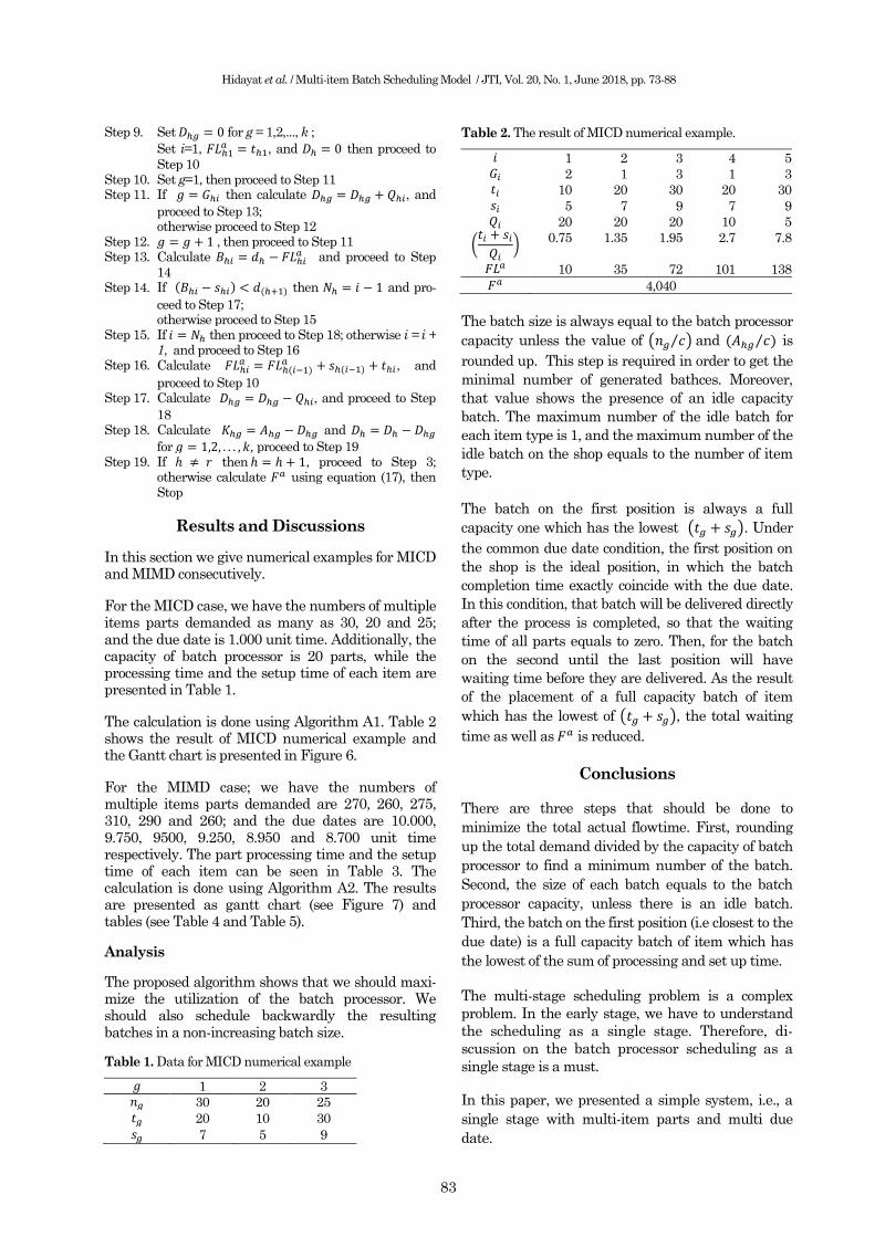
The calculation is done using Algorithm A1. Table 2 shows the result of MICD numerical example and the Gantt chart is presented in Figure 6.

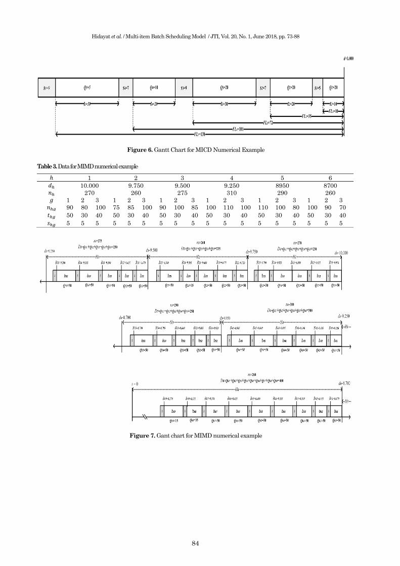
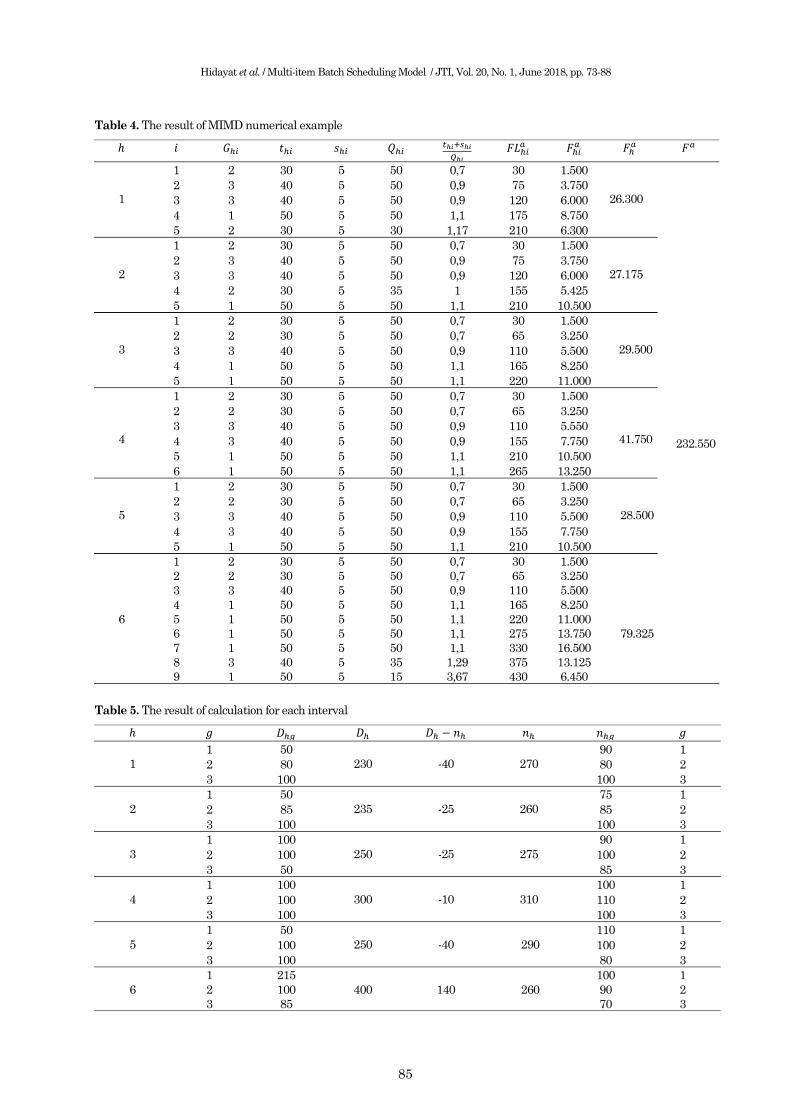
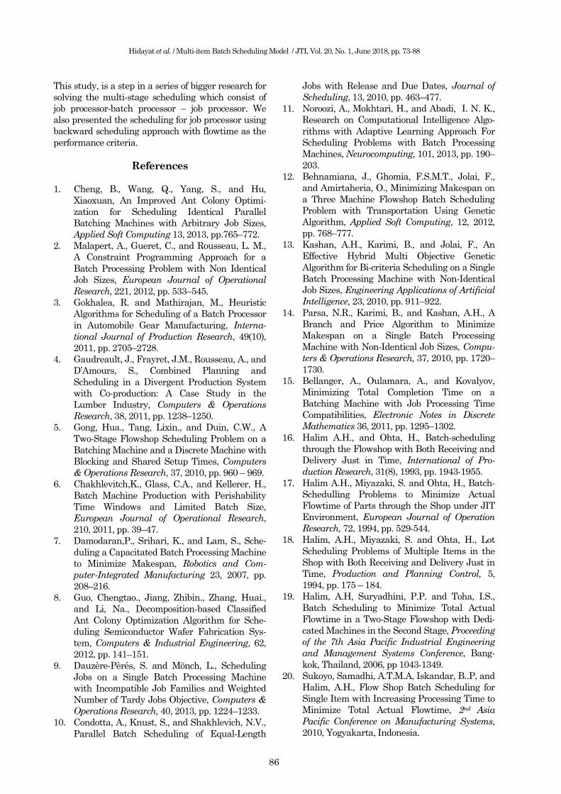
For the MIMD case; we have the numbers of multiple items parts demanded are 270, 260, 275, 310, 290 and 260; and the due dates are 10.000, 9.750, 9500, 9.250, 8.950 and 8.700 unit time respectively. The part processing time and the setup time of each item can be seen in Table 3. The calculation is done using Algorithm A2. The results are presented as gantt chart (see Figure 7) and tables (see Table 4 and Table 5).

Analysis

The proposed algorithm shows that we should maxi-mize the utilization of the batch processor. We should also schedule backwardly the resulting batches in a non-increasing batch size.

Table 1. Data for MICD numerical example

1 2 3 30 20 25

20 10 30

7 5 9

Table 2. The result of MICD numerical example.

1 2 3 4 5 2 1 3 1 3 10 20 30 20 30 5 7 9 7 9 20 20 20 10 5

(

)

0.75 1.35 1.95 2.7 7.8

10 35 72 101 138

4,040

The batch size is always equal to the batch processor

capacity unless the value of ( ⁄ ) and ( ⁄ ) is

rounded up. This step is required in order to get the

minimal number of generated bathces. Moreover,

that value shows the presence of an idle capacity

batch. The maximum number of the idle batch for

each item type is 1, and the maximum number of the

idle batch on the shop equals to the number of item

type.

The batch on the first position is always a full

capacity one which has the lowest ( ). Under

the common due date condition, the first position on

the shop is the ideal position, in which the batch

completion time exactly coincide with the due date.

In this condition, that batch will be delivered directly

after the process is completed, so that the waiting

time of all parts equals to zero. Then, for the batch

on the second until the last position will have

waiting time before they are delivered. As the result

of the placement of a full capacity batch of item

which has the lowest of ( ), the total waiting

time as well as is reduced.

Conclusions

There are three steps that should be done to

minimize the total actual flowtime. First, rounding

up the total demand divided by the capacity of batch

processor to find a minimum number of the batch.

Second, the size of each batch equals to the batch

processor capacity, unless there is an idle batch.

Third, the batch on the first position (i.e closest to the

due date) is a full capacity batch of item which has

the lowest of the sum of processing and set up time.

The multi-stage scheduling problem is a complex

problem. In the early stage, we have to understand

the scheduling as a single stage. Therefore, di-

scussion on the batch processor scheduling as a

single stage is a must.

In this paper, we presented a simple system, i.e., a

single stage with multi-item parts and multi due

date.


84

Figure 6. Gantt Chart for MICD Numerical Example

Table 3. Data for MIMD numerical example

1 2 3 4 5 6

𝑑 10.000 9.750 9.500 9.250 8950 8700 𝑛 270 260 275 310 290 260 𝑔 1 2 3 1 2 3 1 2 3 1 2 3 1 2 3 1 2 3 𝑛 𝑔 90 80 100 75 85 100 90 100 85 100 110 100 110 100 80 100 90 70

𝑡 𝑔 50 30 40 50 30 40 50 30 40 50 30 40 50 30 40 50 30 40

𝑠 𝑔 5 5 5 5 5 5 5 5 5 5 5 5 5 5 5 5 5 5

Figure 7. Gant chart for MIMD numerical example


85

Table 4. The result of MIMD numerical example

𝑖 𝐺 𝑖 𝑡 𝑖 𝑠 𝑖 𝑄 𝑖 𝑡 𝑖 𝑠 𝑖

𝑄 𝑖 𝐹𝐿 𝑖

𝑎 𝐹 𝑖𝑎 𝐹

𝑎 𝐹𝑎

1

1 2 30 5 50 0,7 30 1.500

26.300

232.550

2 3 40 5 50 0,9 75 3.750

3 3 40 5 50 0,9 120 6.000

4 1 50 5 50 1,1 175 8.750

5 2 30 5 30 1,17 210 6.300

2

1 2 30 5 50 0,7 30 1.500

27.175 2 3 40 5 50 0,9 75 3.750

3 3 40 5 50 0,9 120 6.000

4 2 30 5 35 1 155 5.425

5 1 50 5 50 1,1 210 10.500

3

1 2 30 5 50 0,7 30 1.500

29.500 2 2 30 5 50 0,7 65 3.250

3 3 40 5 50 0,9 110 5.500

4 1 50 5 50 1,1 165 8.250

5 1 50 5 50 1,1 220 11.000

4

1 2 30 5 50 0,7 30 1.500

41.750

2 2 30 5 50 0,7 65 3.250

3 3 40 5 50 0,9 110 5.550

4 3 40 5 50 0,9 155 7.750

5 1 50 5 50 1,1 210 10.500

6 1 50 5 50 1,1 265 13.250

5

1 2 30 5 50 0,7 30 1.500

28.500 2 2 30 5 50 0,7 65 3.250

3 3 40 5 50 0,9 110 5.500

4 3 40 5 50 0,9 155 7.750

5 1 50 5 50 1,1 210 10.500

6

1 2 30 5 50 0,7 30 1.500

79.325

2 2 30 5 50 0,7 65 3.250

3 3 40 5 50 0,9 110 5.500

4 1 50 5 50 1,1 165 8.250

5 1 50 5 50 1,1 220 11.000

6 1 50 5 50 1,1 275 13.750

7 1 50 5 50 1,1 330 16.500

8 3 40 5 35 1,29 375 13.125

9 1 50 5 15 3,67 430 6.450

Table 5. The result of calculation for each interval

𝑔 𝐷 𝑔 𝐷 𝐷 𝑛 𝑛 𝑛 𝑔 𝑔

1

1 50

230

-40

270

90 1

2 80 80 2

3 100 100 3

2

1 50

235

-25

260

75 1

2 85 85 2

3 100 100 3

3

1 100

250

-25

275

90 1

2 100 100 2

3 50 85 3

4

1 100

300

-10

310

100 1

2 100 110 2

3 100 100 3

5

1 50

250

-40

290

110 1

2 100 100 2

3 100 80 3

6

1 215

400

140

260

100 1

2 100 90 2

3 85 70 3


86

This study, is a step in a series of bigger research for

solving the multi-stage scheduling which consist of

job processor-batch processor – job processor. We

also presented the scheduling for job processor using

backward scheduling approach with flowtime as the

performance criteria.

References

1. Cheng, B., Wang, Q., Yang, S., and Hu,

Xiaoxuan, An Improved Ant Colony Optimi-

zation for Scheduling Identical Parallel

Batching Machines with Arbitrary Job Sizes,

Applied Soft Computing 13, 2013, pp.765–772.

2. Malapert, A., Gueret, C., and Rousseau, L. M.,

A Constraint Programming Approach for a

Batch Processing Problem with Non Identical

Job Sizes, European Journal of Operational

Research, 221, 2012, pp. 533–545.

3. Gokhalea, R. and Mathirajan, M., Heuristic

Algorithms for Scheduling of a Batch Processor

in Automobile Gear Manufacturing, Interna-

tional Journal of Production Research, 49(10),

2011, pp. 2705–2728.

4. Gaudreault, J., Frayret, J.M., Rousseau, A., and

D’Amours, S., Combined Planning and

Scheduling in a Divergent Production System

with Co-production: A Case Study in the

Lumber Industry, Computers & Operations

Research, 38, 2011, pp. 1238–1250.

5. Gong, Hua., Tang, Lixin., and Duin, C.W., A

Two-Stage Flowshop Scheduling Problem on a

Batching Machine and a Discrete Machine with

Blocking and Shared Setup Times, Computers

& Operations Research, 37, 2010, pp. 960 – 969.

6. Chakhlevitch,K., Glass, C.A., and Kellerer, H.,

Batch Machine Production with Perishability

Time Windows and Limited Batch Size,

European Journal of Operational Research,

210, 2011, pp. 39–47.

7. Damodaran,P., Srihari, K., and Lam, S., Sche-

duling a Capacitated Batch Processing Machine

to Minimize Makespan, Robotics and Com-

puter-Integrated Manufacturing 23, 2007, pp.

208–216.

8. Guo, Chengtao., Jiang, Zhibin., Zhang, Huai.,

and Li, Na., Decomposition-based Classified

Ant Colony Optimization Algorithm for Sche-

duling Semiconductor Wafer Fabrication Sys-

tem, Computers & Industrial Engineering, 62,

2012, pp. 141–151.

9. Dauzère-Pèrés, S. and Mönch, L., Scheduling

Jobs on a Single Batch Processing Machine

with Incompatible Job Families and Weighted

Number of Tardy Jobs Objective, Computers &

Operations Research, 40, 2013, pp. 1224–1233.

10. Condotta, A., Knust, S., and Shakhlevich, N.V.,

Parallel Batch Scheduling of Equal-Length

Jobs with Release and Due Dates, Journal of

Scheduling, 13, 2010, pp. 463–477.

11. Noroozi, A., Mokhtari, H., and Abadi, I. N. K.,

Research on Computational Intelligence Algo-

rithms with Adaptive Learning Approach For

Scheduling Problems with Batch Processing

Machines, Neurocomputing, 101, 2013, pp. 190–

203.

12. Behnamiana, J., Ghomia, F.S.M.T., Jolai, F.,

and Amirtaheria, O., Minimizing Makespan on

a Three Machine Flowshop Batch Scheduling

Problem with Transportation Using Genetic

Algorithm, Applied Soft Computing, 12, 2012,

pp. 768–777.

13. Kashan, A.H., Karimi, B., and Jolai, F., An

Effective Hybrid Multi Objective Genetic

Algorithm for Bi-criteria Scheduling on a Single

Batch Processing Machine with Non-Identical

Job Sizes, Engineering Applications of Artificial

Intelligence, 23, 2010, pp. 911–922.

14. Parsa, N.R., Karimi, B., and Kashan, A.H., A

Branch and Price Algorithm to Minimize

Makespan on a Single Batch Processing

Machine with Non-Identical Job Sizes, Compu-

ters & Operations Research, 37, 2010, pp. 1720–

1730.

15. Bellanger, A., Oulamara, A., and Kovalyov,

Minimizing Total Completion Time on a

Batching Machine with Job Processing Time

Compatibilities, Electronic Notes in Discrete

Mathematics 36, 2011, pp. 1295–1302.

16. Halim A.H., and Ohta, H., Batch-scheduling

through the Flowshop with Both Receiving and

Delivery Just in Time, International of Pro-

duction Research, 31(8), 1993, pp. 1943-1955.

17. Halim A.H., Miyazaki, S. and Ohta, H., Batch-

Schedulling Problems to Minimize Actual

Flowtime of Parts through the Shop under JIT

Environment, European Journal of Operation

Research, 72, 1994, pp. 529-544.

18. Halim, A.H., Miyazaki, S. and Ohta, H., Lot

Scheduling Problems of Multiple Items in the

Shop with Both Receiving and Delivery Just in

Time, Production and Planning Control, 5,

1994, pp. 175 – 184.

19. Halim, A.H, Suryadhini, P.P. and Toha, I.S.,

Batch Scheduling to Minimize Total Actual

Flowtime in a Two-Stage Flowshop with Dedi-

cated Machines in the Second Stage, Proceeding

of the 7th Asia Pacific Industrial Engineering

and Management Systems Conference, Bang-

kok, Thailand, 2006, pp 1043-1349.

20. Sukoyo, Samadhi, A.T.M.A, Iskandar, B..P, and

Halim, A.H., Flow Shop Batch Scheduling for

Single Item with Increasing Processing Time to

Minimize Total Actual Flowtime, 2nd Asia

Pacific Conference on Manufacturing Systems,

2010, Yogyakarta, Indonesia.


87

21. Zahedi, Samadhi, A.T.M.A, Suprayogi, and Halim, A.H., Integrated Batch Production and Maintenance Scheduling for Multiple Items Processed on a Deteriorating Machine to Mini-mize Total Production and Maintenance Cost with Due-date Constraint, International Jour-nal of Industrial Engineering Computation, 7, 2016, pp.229-244.

22. Hidayat, N.P.A., Cakravastia A., Samadhi, A. TMA., Halim, A.H., A Single Item Batch Scheduling Model on a Batch Processor to Minimize Total Actual Flowtime of Parts Through the Shop, Proceeding Asia Pacific Industrial Engineering and Management System, Cebu Island, Philipina, 2013.

23. Hidayat, N. P.A., Cakravastia A., Samadhi, A.

TMA., and Halim, A.H., A Batch-scheduling

Problem to Minimize Total Actual Flowtime of

Parts through the Shop which has m Hetero-

genous Batch Processors, Proceeding Asia

Pacific Industrial Engineering and Mana-

gement System, Jeju Island, South Korea, 2014.

24. Hidayat, N. P.A., Cakravastia A., Samadhi, A.

TMA., and Halim, A.H., A Batch Scheduling

Model for m Heterogeneous Batch Processor,

International of Production Research, 54(4),

2016, pp1170-1185.

25. Halim, A.H., Ernawati, and Hidayat, N. P.A., A

Model of Batch Scheduling for a Single Batch

Processor with Addintional Setups to Minimize

Total Inventory Holding Cost of Parts of a

Single Item Requested at Multi-due-date, Pro-

ceeding Asia Pacific Conference on Manufac-

turing Systems and International Manufac-

turing Engineering Conference, Yogyakarta,

Indonesia, 2017.

Documents

Multi-items Batch Scheduling Model for a Batch Processor