Multi-instance clustering with applications to multi-instance prediction

Appl Intell (2009) 31: 47–68DOI 10.1007/s10489-007-0111-x

Multi-instance clustering with applications to multi-instanceprediction

Min-Ling Zhang · Zhi-Hua Zhou

Published online: 23 January 2008© Springer Science+Business Media, LLC 2007

Abstract In the setting of multi-instance learning, each ob-ject is represented by a bag composed of multiple instancesinstead of by a single instance in a traditional learningsetting. Previous works in this area only concern multi-instance prediction problems where each bag is associatedwith a binary (classification) or real-valued (regression) la-bel. However, unsupervised multi-instance learning wherebags are without labels has not been studied. In this paper,the problem of unsupervised multi-instance learning is ad-dressed where a multi-instance clustering algorithm namedBAMIC is proposed. Briefly, by regarding bags as atomicdata items and using some form of distance metric to mea-sure distances between bags, BAMIC adapts the populark-MEDOIDS algorithm to partition the unlabeled trainingbags into k disjoint groups of bags. Furthermore, based onthe clustering results, a novel multi-instance prediction al-gorithm named BARTMIP is developed. Firstly, each bagis re-represented by a k-dimensional feature vector, wherethe value of the i-th feature is set to be the distance be-tween the bag and the medoid of the i-th group. After that,bags are transformed into feature vectors so that commonsupervised learners are used to learn from the transformedfeature vectors each associated with the original bag’s label.Extensive experiments show that BAMIC could effectivelydiscover the underlying structure of the data set and BART-

M.-L. Zhang · Z.-H. Zhou (�)National Key Laboratory for Novel Software Technology,Nanjing University, Nanjing 210093, Chinae-mail: [email protected]

M.-L. ZhangCollege of Computer and Information Engineering,Hohai University, Nanjing 210098, China

MIP works quite well on various kinds of multi-instanceprediction problems.

Keywords Machine learning · Multi-instance learning ·Clustering · Representation transformation

1 Introduction

Multi-instance learning originated from the study of drugactivity prediction problem. The goal is to endow learningsystems with the ability of predicting that whether a newmolecule could be used to make some drug, through ana-lyzing a collection of known molecules. The qualificationof the molecule to make some drug is determined by someof its shapes with low energy. The main difficulty lies inthat each molecule may have many alternative low-energyshapes while biochemists only know that whether a knownmolecule is qualified to make some drug instead of know-ing that which of its alternative shapes is responsible for thequalification. In order to solve this problem, Dietterich etal. [1] proposed the notion of multi-instance learning, wherethe training set is composed of many bags each containingmany instances.

Previous works on multi-instance learning only deal withprediction tasks where each bag is associated with a binaryor real-valued label. Dietterich et al. [1] studied the standardmulti-instance prediction (STDMIP) problem where a bag ispositively labeled if it contains at least one positive instance;otherwise, it is labeled as a negative bag. The task is to learnsome concept from the training set for correctly labeling un-seen bags. Recently, in addition to the above definition ofSTDMIP, two kinds of generalized multi-instance predic-tion (GENMIP) problems are formalized by Weidmann etal. [2] and Scott et al. [3], respectively. In GENMIP prob-lems, a bag is qualified to be positive if instances in the

mailto:[email protected]

48 M.-L. Zhang, Z.-H. Zhou

bag satisfy some sophisticated constraints other than simplyhaving at least one positive instance. Moreover, besides theabove multi-instance classification problems with discrete-valued (in particular, binary) outputs, multi-instance regres-sion (MIR) problems with real-valued outputs have alsobeen investigated [4–6].

However, unsupervised multi-instance learning wheretraining bags are without labels have not been thoroughlystudied even though it should not be considered less im-portant than multi-instance prediction, i.e. supervised multi-instance learning. There are two main reasons for the ne-cessity of unsupervised multi-instance learning. Firstly, insome cases, it is hard or costly to obtain labels for thebags. For instance, biochemists may easily design variousdrug molecules each represented by a bag whose instancescorrespond to the low-energy shapes of the molecule [1],while it is quite costly to conduct biochemical experimentsin order to determine the functionality (label) of the mole-cule (bag). Therefore, unsupervised multi-instance learningmay help the biochemists identify similar molecules whichmay have similar properties so as to facilitate the drug de-sign process. Secondly, it is well-known that unsupervisedlearning could help find the inherent structure of a data set.Therefore, even for multi-instance prediction tasks wherebags are with labels, it is instructive to initially perform un-supervised multi-instance learning. In this way, some usefulinformation about the data set may be acquired which couldbenefit the following prediction procedure.

Cluster analysis (clustering) is one of the most popu-lar unsupervised learning methods, which is the process ofgrouping a set of physical or abstract objects into classesof similar objects [7]. A good clustering will produce highquality clusters with high intra-class similarity and lowinter-class similarity. It can be used as a stand-alone toolto gain insight into the distribution of data or to serve as apreprocessing step for other tasks. In this paper, the problemof unsupervised multi-instance learning is directly investi-gated where a multi-instance clustering algorithm namedBAMIC, i.e. BAg-level Multi-Instance Clustering, is pro-posed. Concretely, BAMIC tries to partition the unlabeledtraining bags into k disjoint groups of bags, where severalforms of Hausdorff metric [8] are utilized to measure dis-tances between bags with which the popular k-MEDOIDS

algorithm is adapted to fulfill the clustering task. Experi-mental results show that BAMIC could effectively reveal theinherent structure of the multi-instance data set.

In addition, based on the clustering results of BAMIC, anovel multi-instance prediction algorithm named BARTMIP,i.e. BAg-level Representation Transformation for Multi-Instance Prediction, is also developed. Specifically, BART-MIP performs representation transformation by convertingeach bag into a corresponding k-dimensional feature vec-tor whose i-th feature equals the distance between the bag

and the medoid of the i-th group. Consequently, bags aretransformed into feature vectors meaning that the originaltask of multi-instance prediction is reduced to the task oftraditional supervised learning. In this paper, support vectormachines are employed to learn from the reduced learningproblems. Extensive experiments show that the performanceof BARTMIP is highly competitive to those of other multi-instance prediction algorithms on various multi-instanceprediction problems, such as STDMIP, MIR and two kindsof GENMIP models.1

The rest of this paper is organized as follows. Sec-tion 2 briefly reviews previous literatures on multi-instancelearning. Section 3 presents BAMIC and reports its experi-mental results on real-world and artificial data sets. Section 4presents BARTMIP and reports its experimental results onvarious multi-instance prediction problems. Section 5 dis-cusses the relationships between BARTMIP and other relatedworks. Finally, Sect. 6 concludes and raises several issuesfor future work.

2 Literature review

Multi-instance learning originates from the research of drugactivity prediction [1], where the PAC-learnability of thislearning framework has been studied by many researchers.Long and Tan [9] showed that if the instances in the bagsare independently drawn from product distribution, then theAPR (Axis-Parallel Rectangle) proposed by Dietterich et al.[1] is PAC-learnable. Auer et al. [10] showed that if the in-stances in the bags are not independent then APR learningunder the multi-instance learning framework is NP-hard.Moreover, they presented a theoretical algorithm that doesnot require product distribution, which has been transformedto a practical algorithm named MULTINST [11]. Blum andKalai [12] described a reduction from PAC-learning underthe multi-instance learning framework to PAC-learning withone-sided or two-sided random classification noise. Theyalso presented a theoretical algorithm with smaller samplecomplexity than that of the algorithm of Auer et al. [10].Goldman et al. [13] presented an efficient on-line agnos-tic multi-instance learning algorithm for learning the classof constant-dimension geometric patterns, which toleratedboth noise and concept shift. Later, this algorithm was ex-tended so that it could deal with real-valued output [14].

Many practical STDMIP algorithms have been developedduring the past years, such as APR algorithms [1], DIVERSE

DENSITY [15] and its variants [16, 17], multi-instancelazy learning algorithms [18], multi-instance tree learners

1In this paper, the generalized multi-instance prediction model pro-posed by Weidmann et al. [2] is denoted as GENMIP Model I;Accordingly, the other generalized multi-instance prediction modelproposed by Scott et al. [3] is denoted as GENMIP Model II.

Multi-instance clustering with applications to multi-instance prediction 49

[19–21], multi-instance rule inducer [20], multi-instancelogistic regression methods [22], multi-instance neural net-works [23–27], multi-instance kernel methods [28–30], andmulti-instance ensembles [22, 31–34], etc. STDMIP tech-niques have already been applied to diverse applicationsincluding content-based image retrieval [35–39], scene clas-sification [17, 40], stock selection [15], landmark matching[13, 14], computer security [19], subgoal discovery [41],web mining [42], etc.

In the early years of the research of multi-instance learn-ing, most works were on multi-instance classification withdiscrete-valued outputs. Later, multi-instance regressionwith real-valued outputs caught the attention of many re-searchers [4–6].

Besides the STDMIP and MIR problems as introducedabove, two kinds of GENMIP models have also been for-malized recently. Firstly, Weidmann et al. [2] indicatedthat through employing different assumptions of how theinstances’ classifications determine their bag’s label, dif-ferent kinds of multi-instance prediction problems couldbe defined. Formally, let X denote the instance space and� = {0,1} denote the set of class labels. A multi-instanceconcept is a function νMI : 2X → �. In STDMIP, this func-tion is defined as (1), where cI ∈ C is a specific concept froma concept space C defined over X , and X ⊆ X is a set of in-stances.

νMI (X) ⇔ ∃x ∈ X : cI (x) (1)

Based on this characterization, Weidmann et al. [2] definedthree kinds of GENMIP problems, i.e. presence-based MI,2

threshold-based MI, and count-based MI. Presence-basedMI is defined in terms of the presence of instances of eachconcept in a bag, as shown in (2); threshold-based MI re-quires a certain number of instances of each concept to bepresent simultaneously, as defined in (3); count-based MIrequires a maximum as well as a minimum number of in-stances of a certain concept in a bag, as defined in (4).

νPB(X) ⇔ ∀ci ∈ C : �(X,ci) ≥ 1 (2)

νT B(X) ⇔ ∀ci ∈ C : �(X,ci) ≥ ti (3)

νCB(X) ⇔ ∀ci ∈ C : ti ≤ �(X,ci) ≤ zi (4)

In (2) to (4), νPB , νT B and νCB are functions defined on2X → �, C ⊂ C is a given set of concepts, � is a count-ing function � : 2X × C → N which counts the numberof a given concept in a bag, ti ∈ N and zi ∈ N are respec-tively the lower and upper threshold for concept ci . Twoalgorithms have been proposed for this kind of GENMIPmodel (GENMIP Model I), i.e. TLC [2] and CCE [43], both

2Here multi-instance is abbreviated as MI.

of which could also work well in solving STDMIP prob-lems.

Independently of Weidmann et al. [2], Scott et al. [3] de-fined another GENMIP model where the target concept isdefined by two sets of points. Specifically, they defined theirconcepts by a set of q ‘attraction’ points C = {c1, . . . , cq}and a set of q ′ ‘repulsion’ points C = {c1, . . . , cq ′ }. Thenthe label for a bag X = {x1, . . . , xp} is positive if there isa subset of r points C′ ⊆ C ∪ C such that each attractionpoint ci ∈ C′ is near some point in X and each repulsionpoint cj ∈ C′ is not near any point in X. In other words, ifone boolean attribute aci

is defined for each attraction pointci ∈ C which takes the value of 1 if there exists some pointx ∈ X near it, and another boolean attribute acj

is definedfor each repulsion point cj ∈ C which takes the value of 1if there is no point from X near it, then the bag’s label is anr-of-(q + q ′) threshold function over these attributes. Sev-eral algorithms have been specially designed for this kindof GENMIP model (GENMIP Model II), such as GMIL-1[3], GMIL-2 [44], k∧ [45] and kmin [46]. The same as TLC

[2] and CCE [43], these GENMIP algorithms could also beutilized to solve STDMIP problems. In addition, GENMIPModel II has also been applied to applications such as robotvision, content-based image retrieval, binding affinity, andbiological sequence analysis [3].

Note that none of these two GENMIP models is moreexpressive than the other one. For instance, by settingti ≥ 2 (i ∈ {1, . . . , q}) for each attraction point, then boththe threshold-based MI and count-based MI models of Wei-dmann et al. [2] will not be possible to be represented bythe GENMIP model of Scott et al. [3]. On the other hand,as indicated by Tao et al. [45], when r < q + q ′, the repre-sentational ability of Scott et al.’s model will go beyond thegeneralization scope of Weidmann et al.’s. It is also worthnoting that these two GENMIP models do overlap with eachother under certain circumstances. For instance, by settingti = zi = 1 (i ∈ {1, . . . , q}) for each attraction point and set-ting tj = zj = 0 (j ∈ {1, . . . , q ′}) for each repulsion point,then the count-based MI model of Weidmann et al. is justthe one of Scott et al. with r = q + q ′.

It is worth mentioning that multi-instance learning hasalso attracted the attention of the Inductive Logic Program-ming (ILP) community. De Raedt [47] suggested that multi-instance problems could be regarded as a bias on inductivelogic programming, and the multi-instance paradigm couldbe the key between the propositional and relational rep-resentations, being more expressive than the former, andmuch easier to learn than the latter. Recently, Alphonse andMatwin [48] successfully employed multi-instance learningto help relational learning, where the expressive power ofrelational representation and the ease of feature selectionon propositional representation are gracefully combined. Itis also worth noting that although multi-instance learning


was proposed initially based on propositional representa-tion, a recent modification developed by McGovern andJensen [49] allows multi-instance techniques to be used onrelational representation. These works confirm that multi-instance learning can really act as a bridge between propo-sitional and relational learning.

All the works reviewed in this section concern super-vised multi-instance learning where bags are associated withlabels (discrete-valued or real-valued). In the next section,unsupervised multi-instance learning problem where bagsare without labels is addressed by the first multi-instanceclustering algorithm BAMIC.

3 Multi-instance clustering

3.1 BAMIC

Previous works show that multi-instance representation, i.e.bag of multiple instances, seems a natural and appropriateform for object description in many real-world problems.For instance, in drug activity prediction, due to rotationsof internal bonds a drug molecule usually have many low-energy shapes each can be represented by an instance [1];Another example is scene classification, where an imageusually contains multiple regions each of which can be rep-resented as an instance [17, 40]; Web mining is a furtherexample, where each of the links in the web page can be re-garded as an instance [42]. However, although it is relativelyeasy to represent a large number of available objects (e.g.images in databases) by bags of instances via pre-definedbag generation process, obtaining labels for these objectswill be a rather costly and tedious work. In this case, unsu-pervised multi-instance learning techniques could properlymanifest its capability to summarize some useful informa-tion from unlabeled training bags which could be utilizedfor further analysis.

As introduced in Sect. 1, clustering is one of the mostpopular strategies for unsupervised learning. Traditionalclustering schemes include partitioning methods (e.g. k-MEDOIDS), hierarchical methods (e.g. AGNES), density-based methods (e.g. DBSCAN), grid-based methods (e.g.STING), model-based methods (e.g. SOM), etc. [7]. In thispaper, BAMIC adapts the popular k-MEDOIDS algorithm tocomplete the desired multi-instance clustering task due to itssimplicity and efficiency.

Note that at the first glance, multi-instance clusteringmay be regarded as merely a simple extension of traditionalclustering task where the objects to be clustered are nowsets of instances instead of single instances. However, thetask of clustering multi-instance bags has its own charac-teristics. Specifically, in order to cluster objects describedby sets of instances, the most intuitive strategy is to let the

instances contained in one set contribute equally to the clus-tering process. While for multi-instance clustering, this kindof strategy may not be appropriate since the instances com-prising the bag usually exhibit different functionalities. Forexample, only one or few of the low-energy shapes describ-ing one molecule would be responsible for its qualificationto make certain drugs. Similarly, only one or few of theregions describing one image would be useful for certain ap-plications such as scene classification. Therefore, althoughin multi-instance clustering the labels of the bags are miss-ing, the bags should not be regarded as simple collectionsof independent instances while the idiosyncrasies and rela-tionships of the instances in the bags should be carefullyinvestigated.

Let X denote the domain of instances. Suppose thetraining set U is composed of N unlabeled bags, i.e.U = {X1,X2, . . . ,XN } where Xi ⊆ X is a set of instances.BAMIC clusters all the training bags into k disjoint groupsGi (1 ≤ i ≤ k) each containing a number of training bags,i.e.

⋃ki=1 Gi = {X1,X2, . . . ,XN } and Gi

⋂i �=j Gj = ∅.

By regarding each bag as an atomic object, the populark-MEDOIDS algorithm can be easily adapted to fulfill thedesired clustering task provided that some kind of dis-tance function is used to measure the distances betweenbags. Actually, there have been two types of such distances,i.e. maximal Hausdorff distance [8] and minimal Haus-dorff distance [18]. Formally, given two bags of instancesA = {a1, . . . , am} and B = {b1, . . . , bn}, the maximal andminimal Hausdorff distances are defined as (5) and (6) re-spectively, where ‖a − b‖ measures the distance betweeninstances a and b which usually takes the form of Euclideandistance.

maxH(A,B)

= max{

maxa∈A

minb∈B

‖a − b‖,maxb∈B

mina∈A

‖b − a‖}

(5)

minH(A,B) = mina∈A,b∈B

‖a − b‖ (6)

Both maximal and minimal Hausdorff distances have beensuccessfully applied to the STDMIP problems [18] and MIRproblems [4]. However, in our preliminary experiments, itwas found that neither of these two distances could workwell on the GENMIP problems. The reason that maximalHausdorff distance did not work well may be its sensitivityto outlying points [18], while the reason for the unsatis-factory performance of minimal Hausdorff distance may bethat it only considers the distance between the nearest pairof instances in A and B . Therefore, in this paper, anotherdistance called average Hausdorff distance3 is proposed tomeasure the distance between two bags:

3Actually, aveH(·, ·) doesn’t satisfy the triangle inequality and thuscan not be regarded as a metric distance [62]. For instance, let A = {1},B = {2} and C = {1,2}, then aveH(A,C) + aveH(C,B) = 2

3 < 1 =


[Groups, Medoids] = BAMIC(U , k, Bag_dist)

Inputs:U – unlabeled multi-instance training set {X1,X2, . . . ,XN } (Xi ⊆ X )

k – number of clustered groupsBag_dist – distance metric used to calculate distances between bags, which could take the form of maximal, minimal or

average Hausdorff distance in this paper

Outputs:Groups – clustering outputs {G1,G2, . . . ,Gk} (

⋃ki=1 Gi = U , Gi

⋂i �=j Gj = ∅)

Medoids – Medoids of clustered groups

Process:(1) Randomly select k training bags as the initial medoids Cj (1 ≤ j ≤ k);(2) repeat(3) for j ∈ {1,2, . . . , k} do(4) Gj = {Cj };(5) for i ∈ {1,2, . . . ,N} do(6) index = arg minj∈{1,2,...,k} Bag_dist(Xi,Cj );(7) Gindex = Gindex ∪ {Xi};(8) for j ∈ {1,2, . . . , k} do

(9) Cj = arg minA∈Gj

(∑B∈Gj

Bag_dist(A,B)/|Gj |)

;

(10) until {the clustering results do not change};(11) Groups = {Gj |1 ≤ j ≤ k}; Medoids = {Cj |1 ≤ j ≤ k};

Fig. 1 Pseudo-code describing the BAMIC algorithm

aveH(A,B)

=∑

a∈A minb∈B ‖a − b‖ + ∑b∈B mina∈A ‖b − a‖

|A| + |B| (7)

where | · | measures the cardinality of a set. In words,aveH(·, ·) averages the distances between each instance inone bag and its nearest instance in the other bag. Con-ceptually speaking, average Hausdorff distance takes moregeometric relationships between two bags of instances intoconsideration than those of maximal and minimal Hausdorffdistances.

Figure 1 illustrates the complete description of BAMIC.Based on some specific form of Hausdorff distance (max-imal, minimal or average), BAMIC partitions the unlabeledtraining set into k disjoint groups each containing a numberof training bags. The medoid of each group is the one whichhas the minimum average distance to the other bags in thesame group.

aveH(A,C). However, considering that minH(·, ·) is neither a metricdistance (minH(A,C) + minH(C,B) = 0 < 1 = minH(A,C)) but isstill called as minimal Hausdorff distance in the literature [18]. Fol-lowing the same naming style, aveH(·, ·) is called as average Hausdorffdistance in this paper.

3.2 Experiments

3.2.1 Experimental setup

To the best of the authors’ knowledge, BAMIC is the firstwork on unsupervised multi-instance learning, and there isno benchmark data set for the evaluation of unsupervisedmulti-instance learning algorithms. In this paper, several su-pervised multi-instance data sets are employed instead totest the effectiveness of BAMIC. Traditionally, the quality ofthe clustering results is usually measured by various clustervalidation indices [50], where the desired grouping prop-erties such as the labeling information are not available.However, for the experiments reported in this subsection,the labels associated with the bags are known, which canbe utilized to give more realistic estimate of the clusteringquality other than using cluster validation indices.

Considering that no other multi-instance clustering meth-ods are available for comparative studies, the performanceof BAMIC is evaluated against two traditional clusteringmethods, i.e. the partitioning method k-MEDOIDS and thehierarchical method AGNES (AGglomerative NESting, alsoknown as the single-linkage clustering) [7].

Let S be a set of N binary labeled bags, i.e. S ={(X1,BLX1), (X2,BLX2), . . . , (XN,BLXN

)} where Xi ⊆X is a set of instances and BLXi

∈ {0,1} is the binary label


associated with Xi . As shown in Fig. 1, given parametersk (number of clustered groups) and Bag_dist(·, ·) (distancemetric between bags), BAMIC will partition the set of unla-beled bags {X1,X2, . . . ,XN } into k disjoint groups Gj eachcontaining a number of bags. However, as for k-MEDOIDS

and AGNES, both of which cluster the data set at the level ofinstances instead of at the level of bags. In this way, the bagXi may be broken into several parts each belonging to differ-ent group when the clustering process is completed. In orderto account for the effect of fractional bags, each instance inthe bag Xi is now assigned with a weight 1

|Xi | . By doing this,instances from small bags will have higher weights than in-stances from large bags while bags are considered to be ofequal importance (i.e. with weight 1). Note that this kindof weighting strategy has been shown to be reasonable formulti-instance learning as in the literatures [2, 21].

For each group Gj (1 ≤ j ≤ k), let Wlj (l ∈ {0,1}) de-

note the sum of weights of those instances in Gj which arecoming from bags (may be fractional for k-MEDOIDS andAGNES) with label l. Furthermore, let Wj denote the sum ofweights of all the instances in Gj , i.e. Wj = W 0

j + W 1j . It is

easy to see that∑k

j=1 Wj = N . Based on this, the followingtwo criteria are defined in this paper to assess the quality ofthe clustering results:

avgpurity({G1,G2, . . . ,Gk})

=k∑

j=1

Wj

N· max{W 0

j ,W 1j }

Wj

(8)

avgentropy({G1,G2, . . . ,Gk})

=k∑

j=1

Wj

N·⎛

⎝∑

l∈{0,1}−Wl

j

Wj

log2

Wlj

Wj

⎞

⎠ (9)

The first criterion avgpurity(·) measures the weighted av-erage purity of the clustering results. Here, purity of Gj

refers to the ratio of the weights of (fractional) bags be-longing to the dominating class in Gj to the total weights

of (fractional) bags in Gj , which is then weighted byWj

N.

The performance is perfect when avgpurity({G1,G2, . . . ,

Gk}) = 1. The bigger the value of this criterion, the bet-ter the performance of the clustering algorithm; The secondcriterion avgentropy(·) measures the average entropy of theclustering results, i.e. the information needed to correctly

classify all the (fractional) bags in the clustered groups. Itresembles the entropy definition used in traditional deci-sion tree building [51]. The performance is perfect whenavgentropy({G1,G2, . . . ,Gk}) = 0. The smaller the valueof this criterion, the better the performance of the clusteringalgorithm.

Experimental results on several STDMIP and GENMIPdata sets are reported in the following two subsections re-spectively.

3.2.2 STDMIP data sets

MUSK data is a real-world benchmark test data for STDMIPalgorithms, which was generated in the research of drug ac-tivity prediction [1]. Here each molecule is regarded as abag, and its alternative low-energy shapes are regarded asthe instances in the bag. A positive bag corresponds to amolecule qualified to make a certain drug, that is, at leastone of its low-energy shapes could tightly bind to the tar-get area of some larger protein molecules such as enzymesand cell-surface receptors. A negative bag corresponds to amolecule unqualified to make a certain drug, that is, none ofits low-energy shapes could tightly bind to the target area.In order to represent the shapes, a molecule was placed at astandard position and orientation and then a set of 162 raysemanating from the origin was constructed so that the mole-cule surface was sampled approximately uniformly. Therewere also four features representing the position of an oxy-gen atom on the molecular surface. Therefore each instancein the bags was represented by 166 continuous attributes.

There are two data sets, i.e. MUSK1 and MUSK2, bothpublicly available at the UCI machine learning reposi-tory [52]. MUSK1 contains 47 positive bags and 45 negativebags, and the number of instances contained in each bagranges from 2 to 40. MUSK2 contains 39 positive bags and63 negative bags, and the number of instances contained ineach bag ranges from 1 to 1,044. Detailed information onthe MUSK data is tabulated in Table 1.

Figures 2 and 3 show how the performance of each clus-tering algorithm on the MUSK data changes as the numberof clustered groups increasing in terms of average purityand average entropy respectively. The number of clusteredgroups ranges from 5 to 90 on MUSK1 while from 5 to100 on MUSK2, both with an interval of 5. BAMIC-w-minHdenotes the version of BAMIC when minimal Hausdorff

Table 1 The MUSK data (72molecules are shared in bothdata sets)

Data set Dim. Bags Instances Instances per bag

Total MUSK Non-MUSK Min Max Ave.

MUSK1 166 92 47 45 476 2 40 5.17

MUSK2 166 102 39 63 6,598 1 1,044 64.69


distance is used to measure distance between bags. Thesame naming rule goes for BAMIC-w-maxH and BAMIC-w-aveH. For each of the five clustering algorithms, whenthe number of clustered groups is fixed, experiments are re-peated for ten times where the averaged evaluation value outof ten runs is depicted as a point in the figure. The con-crete experimental results of each clustering algorithm interms of average purity and average entropy are also re-ported in Tables 2 and 3 respectively, where the numberof clustered groups ranges from 5 to 80 with an inter-val of 15. The value following ‘±’ gives the standarddeviation and the best result out of the five clustering algo-rithms on each number of clustered groups is shown in boldface.

Figure 2 and Table 2 show that in terms of averagepurity, on both MUSK1 and MUSK2, all the three ver-sions of BAMIC significantly and consistently outperformk-MEDOIDS and AGNES. Furthermore, there is no signifi-cant difference among the performance of the three versions

of BAMIC on MUSK1, while the performance of BAMIC-w-aveH is slightly inferior to those of BAMIC-w-minH andBAMIC-w-maxH on MUSK2. Figure 3 and Table 3 revealthe same phenomena as shown above when the performanceof clustering algorithm is evaluated in terms of average en-tropy. The above results indicate that BAMIC could workwell on the real-world MUSK data.

3.2.3 GENMIP data sets

In addition to the above STDMIP data sets, severalGENMIP data sets are employed to further evaluate theperformance of each clustering algorithm. Specifically, thepresence-based MI of GENMIP Model I proposed by Wei-dmann et al. [2] is used.

In generating presence-based MI data sets, |C| con-cepts were used. To generate a positive bag, the num-ber of instances in a concept ci was chosen randomlyfrom {1, . . . ,10} for each concept. The number of ran-dom instances was selected with equal probability from

Fig. 2 The average purity of the clustering algorithm changes as the number of clustered groups increasing. a MUSK1; b MUSK2

Table 2 Experimental resultsof each clustering algorithm(mean±std) on MUSK1 andMUSK2 with different numberof clustered groups in terms ofaverage purity

Data Clustering Number of clustered groups

set algorithm k = 5 k = 20 k = 35 k = 50 k = 65 k = 80

MUSK1 BAMIC-w-minH .613±.043 .815±.029 .867±.016 .926±.022 .964±.019 .980±.014

BAMIC-w-maxH .644±.038 .828±.036 .869±.028 .905±.017 .945±.020 .974±.013

BAMIC-w-aveH .587±.016 .812±.050 .867±.027 .902±.026 .942±.015 .978±.013

k-MEDOIDS .611±.030 .729±.025 .757±.015 .796±.025 .818±.020 .828±.019

AGNES .571±.000 .666±.000 .746±.000 .767±.000 .771±.000 .795±.000

MUSK2 BAMIC-w-minH .657±.032 .786±.026 .838±.014 .897±.017 .920±.030 .953±.008

BAMIC-w-maxH .649±.020 .777±.022 .846±.021 .901±.022 .923±.017 .960±.019

BAMIC-w-aveH .637±.013 .769±.012 .800±.012 .850±.037 .884±.020 .930±.018

k-MEDOIDS .621±.010 .686±.027 .725±.020 .735±.020 .751±.019 .767±.012

AGNES .618±.000 .618±.000 .665±.000 .678±.000 .731±.000 .733±.000


Fig. 3 The average entropy of the clustering algorithm changes as the number of clustered groups increasing. a MUSK1; b MUSK2

Table 3 Experimental results of each clustering algorithm (mean±std) on MUSK1 and MUSK2 with differ-ent number of clustered groups in terms of average entropy



MUSK1 BAMIC-w-minH .928±.054 .530±.049 .350±.034 .187±.044 .080±.038 .042±.032

BAMIC-w-maxH .886±.060 .481±.082 .341±.067 .236±.047 .127±.045 .056±.026

BAMIC-w-aveH .953±.034 .513±.088 .369±.062 .245±.056 .141±.041 .050±.030

k-MEDOIDS .943±.035 .729±.028 .652±.020 .571±.066 .506±.038 .467±.029

AGNES .935±.000 .816±.000 .667±.000 .626±.000 .618±.000 .579±.000

MUSK2 BAMIC-w-minH .854±.044 .587±.068 .427±.027 .251±.032 .188±.072 .107±.019

BAMIC-w-maxH .897±.018 .578±.053 .395±.045 .251±.046 .187±.038 .091±.037

BAMIC-w-aveH .899±.031 .667±.027 .542±.021 .393±.070 .296±.030 .178±.036

k-MEDOIDS .933±.016 .803±.040 .731±.023 .710±.029 .677±.027 .652±.028

AGNES .910±.000 .810±.000 .773±.000 .743±.000 .665±.000 .651±.000

{10|C|, . . . ,10|C| + 10}. To form a negative bag, they re-placed all instances of a concept ci by random instances.Hence the minimal bag size in this data set was |C| + 10|C|and the maximal bag size was 20|C| + 10. It is obvious thatSTDMIP problem is just a special case of presence-basedMI by using only one underlying concept (i.e. |C| = 1).Therefore, learning from presence-based MI data sets wouldbe inevitably more difficult than learning from STDMIPdata sets such as the MUSK data.

In this paper, four presence-based MI data sets are used,i.e. 2-5-5, 2-10-0, 3-5-5, 3-5-10. Here the name of the dataset ‘2-5-5’ means it was generated with 2 concepts, 5 rele-vant and 5 irrelevant attributes. The same naming rule goesfor the other data sets. In each data set, there are five differ-ent training sets containing 50 positive bags and 50 negativebags, and a big test set containing 5,000 positive bags and5,000 negative bags. When the data set is used to evaluate

the performance of a supervised multi-instance algorithm(as shown in Sect. 4.2.4), the average test set accuracy ofthe classifiers trained on each of these five training sets isrecorded as the predictive accuracy of the tested algorithmon that data set. In this subsection, however, only the fivetraining sets contained in each data set are used to evaluatedthe performance of the unsupervised multi-instance cluster-ing algorithms.

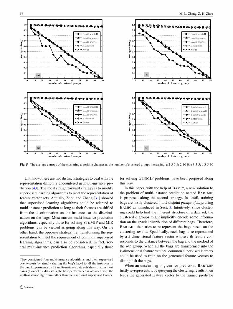
Figures 4 and 5 show how the performance of each clus-tering algorithm on the presence-based MI data sets changesas the number of clustered groups increasing in terms of av-erage purity and average entropy respectively. The numberof clustered groups ranges from 5 to 100 with an intervalof 5 on all data sets. When the number of clustered groupsand the clustering algorithm are fixed, the averaged evalua-tion value out of five training sets is depicted as a point in thefigure. The concrete experimental results of each clustering


Fig. 4 The average purity of the clustering algorithm changes as the number of clustered groups increasing. a 2-5-5; b 2-10-0; c 3-5-5; d 3-5-10

algorithm in terms of average purity and average entropy arealso reported in Tables 4 and 5 respectively, where the num-ber of clustered groups ranges from 5 to 80 with an intervalof 15. The value following ‘±’ gives the standard deviationand the best result out of the five clustering algorithms oneach number of clustered groups is shown in bold face.

As shown by Figs. 4 and 5 together with Tables 4 and 5,on all data sets and evaluation criteria, all the three ver-sions of BAMIC significantly and consistently outperformk-MEDOIDS and AGNES. Specifically, both k-MEDOIDS

and AGNES totally fail to find the inherent structure of theconcerned GENMIP data. Furthermore, on all data sets andevaluation criteria, the performance of BAMIC-w-aveH issuperior to those of BAMIC-w-minH and BAMIC-w-maxH,while there is no significant difference between the per-formance of the latter two versions of BAMIC. The aboveresults show that in addition to the STDMIP data as shownin Sect. 3.2.2, BAMIC (especially BAMIC-w-aveH) couldalso work well on the more complicated GENMIP data.

4 Applications to multi-instance prediction

4.1 BARTMIP

The difficulty of multi-instance prediction (whetherSTDMIP, MIR or GENMIP) mainly lies in that althoughthe training bags are labeled, the labels of their instancesare unknown. Actually, a bag corresponds to a real-worldobject while the instances correspond to feature vectorsdescribing the object. In contrast to typical machine learn-ing settings where an object is represented by one featurevector, in multi-instance learning an object is representedby a set of feature vectors. Therefore, common supervisedmachine learning methods can hardly be applied. In fact,Dietterich et al. [1] showed that learning algorithms ignor-ing the characteristics of multi-instance problems, such aspopular decision trees and neural networks, could not workwell in this scenario.4

4Recently, Ray and Craven [61] empirically studied the relationshipbetween traditional supervised learning and multi-instance learning.


Fig. 5 The average entropy of the clustering algorithm changes as the number of clustered groups increasing. a 2-5-5; b 2-10-0; c 3-5-5; d 3-5-10

Until now, there are two distinct strategies to deal with therepresentation difficulty encountered in multi-instance pre-diction [43]. The most straightforward strategy is to modifysupervised learning algorithms to meet the representation offeature vector sets. Actually, Zhou and Zhang [31] showedthat supervised learning algorithms could be adapted tomulti-instance prediction as long as their focuses are shiftedfrom the discrimination on the instances to the discrimi-nation on the bags. Most current multi-instance predictionalgorithms, especially those for solving STDMIP and MIRproblems, can be viewed as going along this way. On theother hand, the opposite strategy, i.e. transforming the rep-resentation to meet the requirement of common supervisedlearning algorithms, can also be considered. In fact, sev-eral multi-instance prediction algorithms, especially those

They considered four multi-instance algorithms and their supervisedcounterparts by simply sharing the bag’s label to all the instances inthe bag. Experiments on 12 multi-instance data sets show that, in mostcases (8 out of 12 data sets), the best performance is obtained with themulti-instance algorithm rather than the traditional supervised learner.

for solving GENMIP problems, have been proposed alongthis way.

In this paper, with the help of BAMIC, a new solution tothe problem of multi-instance prediction named BARTMIP

is proposed along the second strategy. In detail, trainingbags are firstly clustered into k disjoint groups of bags usingBAMIC as introduced in Sect. 3. Intuitively, since cluster-ing could help find the inherent structure of a data set, theclustered k groups might implicitly encode some informa-tion on the spacial distribution of different bags. Therefore,BARTMIP then tries to re-represent the bags based on theclustering results. Specifically, each bag is re-representedby a k-dimensional feature vector whose i-th feature cor-responds to the distance between the bag and the medoid ofthe i-th group. When all the bags are transformed into thek-dimensional feature vectors, common supervised learnerscould be used to train on the generated feature vectors todistinguish the bags.

When an unseen bag is given for prediction, BARTMIP

firstly re-represents it by querying the clustering results, thenfeeds the generated feature vector to the trained predictor


Table 4 Experimental resultsof each clustering algorithm(mean±std) on presence-basedMI data sets with differentnumber of clustered groups interms of average purity



2-5-5 BAMIC-w-minH .564±.021 .658±.042 .716±.027 .796±.024 .856±.023 .900±.007

BAMIC-w-maxH .538±.019 .636±.013 .690±.012 .768±.016 .842±.008 .906±.006

BAMIC-w-aveH .622±.048 .772±.042 .838±.051 .876±.015 .906±.020 .954±.017

k-MEDOIDS .548±.008 .542±.012 .556±.001 .566±.008 .569±.005 .577±.009

AGNES .503±.001 .509±.001 .513±.001 .520±.003 .524±.004 .530±.004

2-10-0 BAMIC-w-minH .540±.021 .630±.017 .702±.049 .782±.028 .830±.017 .908±.008

BAMIC-w-maxH .558±.026 .656±.025 .700±.014 .794±.020 .854±.018 .908±.005

BAMIC-w-aveH .672±.062 .764±.051 .830±.020 .870±.027 .902±.025 .952±.013

k-MEDOIDS .538±.021 .595±.007 .597±.007 .601±.007 .602±.009 .607±.007

AGNES .501±.001 .507±.001 .531±.027 .558±.010 .561±.011 .563±.010

3-5-5 BAMIC-w-minH .532±.008 .624±.017 .688±.013 .762±.008 .832±.013 .908±.008

BAMIC-w-maxH .542±.015 .634±.018 .710±.022 .778±.016 .844±.021 .918±.015

BAMIC-w-aveH .628±.043 .736±.011 .812±.024 .842±.039 .878±.023 .930±.016

k-MEDOIDS .519±.026 .533±.016 .551±.014 .557±.007 .559±.011 .561±.008

AGNES .501±.001 .506±.001 .511±.001 .516±.002 .521±.001 .526±.002

3-5-10 BAMIC-w-minH .590±.024 .674±.034 .730±.036 .798±.022 .848±.026 .912±.016

BAMIC-w-maxH .554±.017 .618±.018 .720±.026 .770±.024 .862±.034 .924±.027

BAMIC-w-aveH .590±.024 .712±.046 .784±.049 .844±.032 .884±.033 .922±.018

k-MEDOIDS .531±.011 .548±.010 .548±.006 .560±.003 .562±.007 .565±.006

AGNES .501±.000 .503±.001 .504±.001 .506±.001 .507±.001 .509±.000

to obtain the predicted label. This means the clustering re-

sults, at least the medoids of each clustered groups, should

be stored for prediction so that the unseen bag can be

transformed into the corresponding feature vector through

measuring its distance to different group medoids. How-

ever, although BARTMIP is not so efficient as multi-instance

prediction algorithms that do not query on training bags in

prediction, such as RELIC [19], it is more efficient than algo-

rithms that require storing and querying all the training bags

in prediction, such as CITATION-KNN and BAYESIAN-KNN

[18]. As will be shown in the next subsection, a promi-

nent advantage of BARTMIP is that it can be easily applied

to MIR problems by simply replacing the binary classifier

built on the transformed feature vectors with a regression

estimator, and applied to GENMIP problems without any

modification, while most current multi-instance prediction

algorithms can not.

Let D be the set of labeled training bags, i.e. D ={(X1,LX1), (X2,LX2), . . . , (XN,LXN

)} where Xi ⊆ X is a

set of instances and LXiis the label (binary or real-valued)

associated with Xi . The complete description of BARTMIP is

illustrated in Fig. 6. Based on BAMIC, steps (1) to (2) cluster

the training set into k disjoint groups.5 After that, steps (3)to (8) firstly convert each training bag into one feature vec-tor associated with the bag’s label, and then use the givenlearning algorithm to train a predictor from the transformedfeature vectors. Note that many algorithms can be used toimplement the learning algorithm. Finally, steps (9) to (11)output the label for the test bag by feeding the generatedfeature vector to the learned predictor.

Note that although BARTMIP is designed along one exist-ing strategy, i.e. performing representation transformation tomeet the requirement of traditional supervised learning algo-rithms, it has its own characteristics. Firstly, for all the othermulti-instance prediction algorithms based on representa-tion transformation [2, 3, 43–46], the bags are transformedinto corresponding feature vectors by structuring the in-put space at the level of instances. While for BARTMIP,through unsupervised clustering of training bags, represen-tation transformation is performed by structuring the inputspace at the level of bags, which seems more pertinent tothe original representation of multi-instance learning. Onthe other hand, most existing multi-instance prediction al-gorithms have only been applied to one or two kinds of

5In our experiments reported in the next subsection, the clusteringprocess converges within 5 rounds in most cases.


Table 5 Experimental resultsof each clustering algorithm(mean±std) on presence-basedMI data sets with differentnumber of clustered groups interms of average entropy



2-5-5 BAMIC-w-minH .955±.021 .793±.042 .646±.027 .492±.024 .346±.023 .217±.007

BAMIC-w-maxH .961±.019 .799±.013 .661±.012 .502±.016 .358±.008 .206±.006

BAMIC-w-aveH .935±.048 .608±.042 .443±.051 .336±.015 .219±.020 .097±.017

k-MEDOIDS .991±.008 .990±.012 .984±.001 .977±.008 .972±.005 .968±.009

AGNES .999±.001 .994±.001 .991±.001 .985±.003 .981±.004 .977±.004

2-10-0 BAMIC-w-minH .959±.021 .786±.017 .653±.049 .492±.028 .361±.017 .207±.008

BAMIC-w-maxH .956±.026 .790±.025 .668±.014 .487±.020 .341±.018 .211±.005

BAMIC-w-aveH .837±.062 .655±.051 .447±.020 .335±.027 .232±.025 .105±.013

k-MEDOIDS .994±.021 .963±.007 .958±.007 .953±.007 .950±.009 .946±.007

AGNES .999±.001 .996±.001 .981±.027 .967±.010 .964±.011 .961±.010

3-5-5 BAMIC-w-minH .966±.008 .809±.017 .662±.013 .508±.008 .362±.013 .207±.008

BAMIC-w-maxH .954±.015 .776±.018 .611±.022 .483±.016 .339±.021 .182±.015

BAMIC-w-aveH .935±.043 .695±.011 .501±.024 .402±.039 .292±.023 .160±.016

k-MEDOIDS .997±.026 .992±.016 .986±.014 .983±.007 .980±.011 .978±.008

AGNES .999±.001 .996±.001 .994±.001 .991±.002 .988±.001 .985±.002

3-5-10 BAMIC-w-minH .952±.024 .824±.034 .665±.036 .514±.022 .389±.026 .221±.016

BAMIC-w-maxH .964±.017 .826±.018 .640±.026 .528±.024 .320±.034 .182±.027

BAMIC-w-aveH .968±.024 .742±.046 .545±.049 .394±.032 .274±.033 .165±.018

k-MEDOIDS .996±.011 .991±.010 .990±.006 .985±.003 .983±.007 .980±.006

AGNES .999±.000 .996±.001 .993±.001 .990±.001 .987±.001 .984±.000

Label = BARTMIP(D, k, Bag_dist, TBag, Learner)

Inputs:D – labeled multi-instance training set {(X1,LX1), (X2,LX2), . . . , (XN,LXN

)} (Xi ⊆ X , LXi∈ {0,1} or [0,1])

k – number of clustered groupsBag_dist – distance metric used to calculate distances between bags, which could take the form of maximal, minimal or

average Hausdorff distance in this paperTBag – test bag (TBag ⊆ X )Learner – common supervised learner for the transformed feature vectors

Outputs:Label – predicted label for the test bag (Label ∈ {0,1} or [0,1])

Process:(1) Set U = {X1,X2, . . . ,XN };(2) [{G1,G2, . . . ,Gk}, {C1,C2, . . . ,Ck}] = BAMIC(U , k, Bag_dist);(3) Set Tr = ∅;(4) for i ∈ {1,2, . . . ,N} do(5) for j ∈ {1,2, . . . , k} do(6) yi

j = Bag_dist(Xi,Cj );

(7) Tr = Tr⋃{(〈yi

1, yi2, . . . , y

ik〉,LXi

)};(8) Predictor(·) = Learner(Tr);(9) for j ∈ {1,2, . . . , k} do

(10) yj = Bag_dist(TBag,Cj );(11) Label = Predictor(〈y1, y2, . . . , yk〉);

Fig. 6 Pseudo-code describing the BARTMIP algorithm


Table 6 Experimental resultsof BARTMIP (mean±std) on theMUSK data with different baselearners, different number ofclustered groups and differentbag distance metrics

Data Prediction Number of clustered groups (= μ× number of training bags)

set algorithm μ = 20% μ = 40% μ = 60% μ = 80% μ = 100%

MUSK1 BARTMIP-SVM-minH 91.1±0.9 91.2±1.5 90.4±0.9 88.7±1.7 90.2±0.0

BARTMIP-SVM-maxH 85.3±1.6 85.1±2.4 84.4±1.3 82.0±2.5 81.5±0.0

BARTMIP-SVM-aveH 92.6±1.0 94.7±1.0 94.1±1.0 92.0±1.4 90.2±0.0

BARTMIP-BNN-minH 77.2±3.7 76.5±2.7 80.8±1.7 76.5±1.3 79.7±0.0

BARTMIP-BNN-maxH 74.6±1.7 77.9±1.3 79.0±4.1 76.8±3.8 77.5±0.0

BARTMIP-BNN-aveH 79.7±4.1 78.9±4.4 84.4±1.7 78.6±3.5 80.8±0.0

BARTMIP-KNN-minH 87.4±1.8 88.9±2.0 86.7±1.8 87.3±1.7 89.1±0.0

BARTMIP-KNN-maxH 81.1±2.7 80.0±2.4 80.8±2.1 81.0±2.2 81.5±0.0

BARTMIP-KNN-aveH 85.7±3.2 86.3±2.8 86.9±1.5 87.3±1.3 88.0±0.0

MUSK2 BARTMIP-SVM-minH 86.7±2.4 88.0±1.1 86.6±1.9 82.6±1.5 82.4±0.0

BARTMIP-SVM-maxH 85.9±1.9 88.2±1.7 87.6±1.2 85.4±1.3 83.3±0.0

BARTMIP-SVM-aveH 90.7±1.7 91.2±1.0 89.8±1.2 87.3±1.4 88.2±0.0

BARTMIP-BNN-minH 74.2±2.8 76.5±2.6 76.8±3.7 78.1±3.2 74.8±0.0

BARTMIP-BNN-maxH 76.5±2.9 79.4±2.5 82.0±3.2 79.1±4.4 80.4±0.0

BARTMIP-BNN-aveH 69.9±2.3 73.2±3.8 75.5±1.0 75.8±3.3 73.9±0.0

BARTMIP-KNN-minH 83.0±1.5 84.6±0.6 83.0±1.5 82.0±0.6 81.4±0.0

BARTMIP-KNN-maxH 80.7±3.2 82.7±0.6 82.0±1.5 81.1±2.0 81.4±0.0

BARTMIP-KNN-aveH 84.6±3.2 84.6±1.5 85.3±1.7 86.6±2.0 85.3±0.0

multi-instance prediction problems. In this paper, BARTMIP

is utilized to solve various kinds of multi-instance predic-tion problems, including STDMIP, MIR and two kinds ofGENMIP problems.

4.2 Experiments

4.2.1 Experimental setup

As shown in Fig. 6, several parameters should be deter-mined in advance to make BARTMIP be a concrete predic-tion algorithm. In this subsection, support vector machines(SVM),6 backpropagation neural networks (BNN) and K-nearest neighbors (KNN) are used respectively as the baselearners to learn from the transformed feature vectors. Con-sidering that after representation transformation, differentmulti-instance learning problems will give rise to differentcommon supervised learning problems, thus the parametersused by each base learner are coarsely tuned for differ-ent data sets to yield comparable performance. For SVM,Gaussian kernels are used with γ -parameter set to be 0.25and C-parameter set to be 3. For BNN, the number of hidden

6Specifically, the Matlab R© version of LIBSVM [60] is used, where theMatlab code is available at http://www.ece.osu.edu/~maj/osu_svm/ orhttp://www.csie.ntu.edu.tw/~cjlin/libsvm/.

neurons is set to be the number of input neurons. For KNN,the number neighbors considered is set to be 3. The follow-ing experiments (as shown in Table 6) on the MUSK data,whose detailed characteristics have already been introducedin Sect. 3.2.2, are performed to determine other parametersof BARTMIP.

Ten times of leave-one-bag-out tests are performed onboth MUSK1 and MUSK2, where the parameter k (i.e. thenumber of clustered groups) ranges from 20% to 100% of|D| (i.e. the number of training bags) with an interval of20%. BARTMIP-SVM-minH denotes the version of BART-MIP where SVM is employed to learn from the transformedfeature vectors and minimal Hausdorff distance is used tomeasure distance between bags. The same naming rule goesfor the other algorithms. The value following ‘±’ gives thestandard deviation and the best result out of three differentdistance measures on each number of clustered groups isshown in bold face.

Table 6 shows that the number of clustered groups doesnot significantly affect the performance of each predictionalgorithm. When the base learner is fixed, in most casesbetter performance is achieved when average Hausdorffdistance is used as the bag distance metric (except BART-MIP-KNN on MUSK1 and BARTMIP-BNN on MUSK2).Furthermore, when the bag distance metric is fixed, in allcases better performance is achieved when SVM is used as

http://www.ece.osu.edu/~maj/osu_svm/

http://www.csie.ntu.edu.tw/~cjlin/libsvm/


Table 7 Comparison of theperformance (%correct ± std) ofeach multi-instance predictionalgorithm on the MUSK data

Prediction algorithm MUSK1 Eval. Prediction algorithm MUSK2 Eval.

BARTMIP 94.1±1.0 LOO BARTMIP 89.8±1.2 LOO

CCE [43] 92.4 LOO CCE [43] 87.3 LOO

TLC [2] 88.7±1.6 10CV TLC [2] 83.1±3.2 10CV

k∧ [45] 82.4 10CV k∧ [45] 77.3 10CV

kmin [46] 82.4 10CV kmin [46] 77.3 10CV

ID APR [1] 92.4 10CV DD-SVM [17] 91.3 10CV

CITATION-KNN [18] 92.4 LOO ID APR [1] 89.2 10CV

BOOSTING [33] 92.0 10CV MITI [21] 88.2 10CV

GFS KDE APR [1] 91.3 10CV MI SVM [28] 88.0±1.0 10OUT

BAG UNIT-BASED RBF [26] 90.3 10CV RBF-MIP [27] 88.0±3.5 LOO

GFS EC APR [1] 90.2 10CV RELIC [19] 87.3 10CV

BAYESIAN-KNN [18] 90.2 LOO BOOSTING [33] 87.1 10CV

RBF-MIP [27] 90.2±2.6 LOO BAG UNIT-BASED RBF [26] 86.6 10CV

DIVERSE DENSITY [15] 88.9 10CV CITATION-KNN [18] 86.3 LOO

MI-NN [23] 88.0 N/A EM-DD [16] 84.9 10CV

RIPPER-MI [20] 88.0 N/A MI-SVM [29] 84.3 10CV

BP-MIP-PCA [25] 88.0 LOO MILOGREGARITH [22] 84.1±1.3 10CV

MIBOOSTING [22] 87.9±2.0 10CV MULTINST [11] 84.0±3.7 10CV

mi-SVM [29] 87.4 10CV MIBOOSTING [22] 84.0±1.3 10CV

MILOGREGARITH [22] 86.7±1.8 10CV mi-SVM [29] 83.6 10CV

MI SVM [28] 86.4±1.1 10OUT BP-MIP-PCA [25] 83.3 LOO

MILOGREGGEOM [22] 85.9±2.2 10CV DIVERSE DENSITY [15] 82.5 10CV

BP-MIP-DD [25] 85.9 LOO BAYESIAN-KNN [18] 82.4 LOO

DD-SVM [17] 85.8 10CV MILOGREGGEOM [22] 82.3±1.2 10CV

EM-DD [16] 84.8 10CV MI-NN [23] 82.0 N/A

MITI [21] 83.7 10CV BP-MIP [24] 80.4 LOO

RELIC [19] 83.7 10CV BP-MIP-DD [25] 80.4 LOO

BP-MIP [24] 83.7 LOO GFS KDE APR [1] 80.4 10CV

MI-SVM [29] 77.9 10CV RIPPER-MI [20] 77.0 N/A

MULTINST [11] 76.7±4.3 10CV GFS EC APR [1] 75.7 10CV

the base learner. Therefore, in the rest of this paper, the re-ported results of BARTMIP are all obtained with μ set to bethe moderate value of 60%, where SVM is employed to learnfrom the transformed feature vectors and average Hausdorffdistance is utilized to measure distance between bags.

Experimental results of BARTMIP on all kinds of multi-instance prediction formalizations, including STDMIP, MIRand GENMIP, are reported sequentially in the followingsubsections. Note that the performance of different algo-rithms have been reported on different data sets. For eachdata set used in this paper, the experimental results of otheralgorithms ever reported on that data set are included forcomparative studies. Furthermore, in Sect. 4.2.3, time com-plexities of BARTMIP and some other algorithms are alsocompared. All the algorithms studied in this paper take thepropositional (i.e. attribute-value) representation language.

4.2.2 STDMIP data sets

Experimental results on the most widely used STDMIPdata sets, i.e. the MUSK data, are shown in this subsec-tion. The performance of BARTMIP (γ = 0.25, C = 3) arepresented in the first part of Table 7. The first part alsocontains the results of those algorithms designed for GEN-MIP Model I (i.e. TLC [2] and CCE [43]) and GENMIPModel II (i.e. k∧ [45] and kmin [46]), which can also workon the MUSK data. The second part contains the results ofother learning algorithms designed for the STDMIP prob-lems. Note that Zhou and Zhang [31] have shown thatensembles of multi-instance learners could achieve betterresults than single multi-instance learners. However, con-sidering that BARTMIP is a single multi-instance learner,the performance of ensembles of multi-instance learnersare not included in Table 7 for fair comparison. The em-


Table 8 Comparison of thepredictive error of eachmulti-instance predictionalgorithm on the MIR data sets

Data set BARTMIP BP-MIP RBF-MIP DIVERSE DENSITY CITATION-KNN

LJ-80.166.1 3.3 18.5 6.6 N/A 8.6

LJ-80.166.1-S 0.0 18.5 18.5 53.3 0.0

LJ-160.166.1 5.4 16.3 5.1 23.9 4.3

LJ-160.166.1-S 0.0 18.5 1.1 0.0 0.0

Table 9 Comparison of thesquared loss of eachmulti-instance predictionalgorithm on the MIR data sets


LJ-80.166.1 0.0102 0.0487 0.0167 N/A 0.0109

LJ-80.166.1-S 0.0075 0.0752 0.0448 0.1116 0.0025

LJ-160.166.1 0.0051 0.0398 0.0108 0.0852 0.0014

LJ-160.166.1-S 0.0039 0.0731 0.0075 0.0052 0.0022

pirical results shown in Table 7 have been obtained bymultiple runs of tenfold cross-validation (10CV), by 1,000runs of randomly leaving out 10 bags and training onthe remaining ones (10OUT), or by leave-one-bag-out test(LOO).7

Table 7 shows that, among the algorithms shown in thefirst part, BARTMIP is comparable to CCE but apparentlybetter than TLC, k∧ and kmin on both MUSK1 and MUSK2.Compared with those algorithms shown in the second part,BARTMIP is comparable to ID APR, CITATION-KNN andBOOSTING but apparently better than the other algorithmson MUSK1, while it is comparable to DD-SVM, ID APR,MITI, MI SVM and RBF-MIP but apparently better than theother algorithms on MUSK2. These observations show thatBARTMIP works quite well on the STDMIP problems.

4.2.3 MIR data sets

In 2001, Amar et al. [4] presented a method for creating arti-ficial MIR data, which was further studied by Dooly et al. [6]in 2002. This method generates an artificial receptor (targetpoint) t at first. Then, artificial molecules (denoted as Xi )with 3-5 instances per bag are generated, with each featurevalue considered as the distance from the origin to the mole-cular surface when all molecules are in the same orientation.Let Xij denote the j -th instance of Xi and Xijk denote thevalue of the k-th feature of Xij . Each feature has a scalefactor sk ∈ [0,1] to represent its importance in the bindingprocess. The binding energy EXi

of Xi to t is calculated as:

EXi= max

Xij ∈Xi

{n∑

k=1

sk · V (tk − Xijk)

}

(10)

7As pointed out by Andrews et al. [29], the EM-DD algorithm [16]seems to use the test data to select the optimal solution obtained frommultiple runs of the algorithm. Thus, the experimental results of EM-DD shown in Table 7 are those given by Andrews et al. [29].

where n is the number of features and

V (u) = 4ε

((σ

u

)12 −(σ

u

)6)

(11)

is called the Lennard-Jones potential [53] for intermolecu-lar interactions with parameters ε (the depth of the potentialwell) and σ (the distance at which V (u) = 0), and u is thedistance between the bag instances and the target point ona specific feature (they assumed that u > σ which meansV (u) < 0). Based on this, the real-valued label RLXi

∈[0,1] for molecule Xi is the ratio of EXi

to the maximumpossible binding energy Emax:

RLXi= EXi

Emax= max

Xij ∈Xi

{∑nk=1 sk · V (tk − Xijk)

Emax

}

(12)

where Emax = −ε · ∑nk=1 sk . Thresholding at 1/2 converts

RLXito a binary label BLXi

.The artificial data sets are named as LJ-r.f.s where r is the

number of relevant features, f is the number of features, ands is the number of different scale factors used for the rele-vant features. To partially mimic the MUSK data, some datasets only use labels that are not near 1/2 (indicated by the ‘S’suffix) and all scale factors for the relevant features are ran-domly selected between [0.9, 1]. Note that these data sets aremainly designed for multi-instance regression, but they canalso be used for multi-instance classification through round-ing the real-valued label to 0 or 1.

Leave-one-bag-out test is performed on four artificialdata sets, i.e. LJ-80.166.1, LJ-80.166.1-S, LJ-160.166.1 andLJ-160.166.1-S. Each data set contains 92 bags. The perfor-mance of BARTMIP (γ = 1, C = 1) is compared with thoseof BP-MIP, RBF-MIP, DIVERSE DENSITY and CITATION-KNN, where the performance of BP-MIP, RBF-MIP andthose of DIVERSE DENSITY and CITATION-KNN are re-ported in [24], [27] and [4] respectively. Table 8 and Table 9gives the predictive error and squared loss of each compar-ing algorithm.


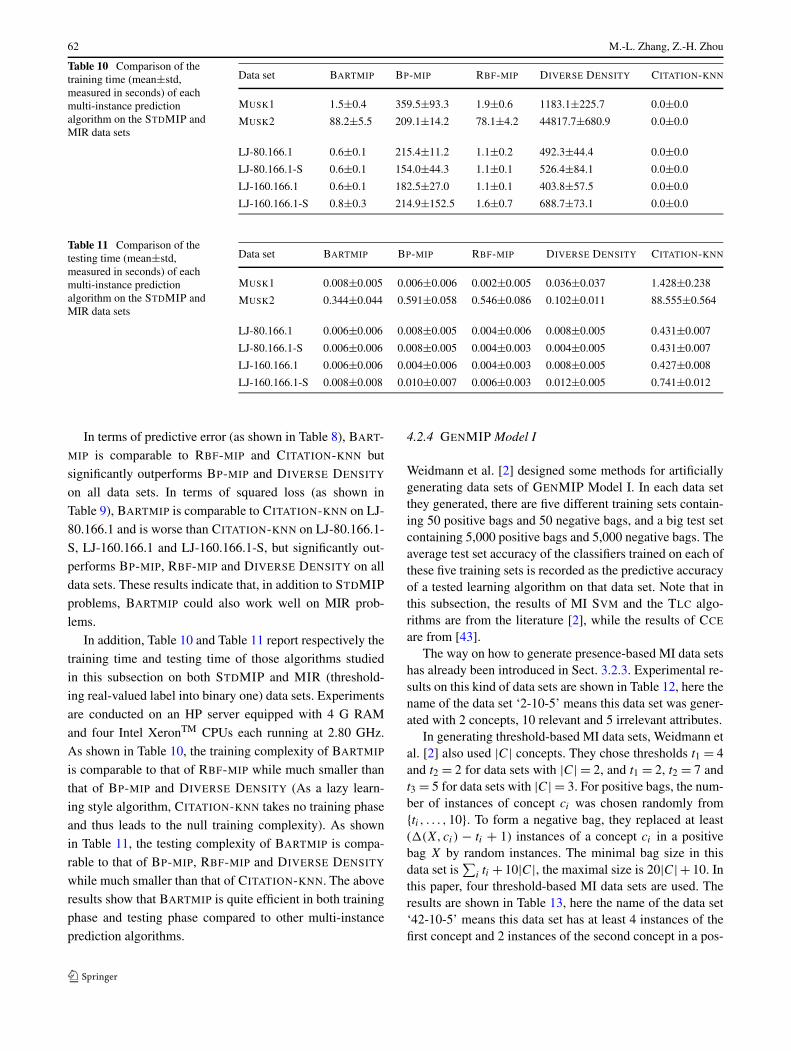
Table 10 Comparison of thetraining time (mean±std,measured in seconds) of eachmulti-instance predictionalgorithm on the STDMIP andMIR data sets


MUSK1 1.5±0.4 359.5±93.3 1.9±0.6 1183.1±225.7 0.0±0.0

MUSK2 88.2±5.5 209.1±14.2 78.1±4.2 44817.7±680.9 0.0±0.0

LJ-80.166.1 0.6±0.1 215.4±11.2 1.1±0.2 492.3±44.4 0.0±0.0

LJ-80.166.1-S 0.6±0.1 154.0±44.3 1.1±0.1 526.4±84.1 0.0±0.0

LJ-160.166.1 0.6±0.1 182.5±27.0 1.1±0.1 403.8±57.5 0.0±0.0

LJ-160.166.1-S 0.8±0.3 214.9±152.5 1.6±0.7 688.7±73.1 0.0±0.0

Table 11 Comparison of thetesting time (mean±std,measured in seconds) of eachmulti-instance predictionalgorithm on the STDMIP andMIR data sets


MUSK1 0.008±0.005 0.006±0.006 0.002±0.005 0.036±0.037 1.428±0.238

MUSK2 0.344±0.044 0.591±0.058 0.546±0.086 0.102±0.011 88.555±0.564

LJ-80.166.1 0.006±0.006 0.008±0.005 0.004±0.006 0.008±0.005 0.431±0.007

LJ-80.166.1-S 0.006±0.006 0.008±0.005 0.004±0.003 0.004±0.005 0.431±0.007

LJ-160.166.1 0.006±0.006 0.004±0.006 0.004±0.003 0.008±0.005 0.427±0.008

LJ-160.166.1-S 0.008±0.008 0.010±0.007 0.006±0.003 0.012±0.005 0.741±0.012

In terms of predictive error (as shown in Table 8), BART-

MIP is comparable to RBF-MIP and CITATION-KNN butsignificantly outperforms BP-MIP and DIVERSE DENSITY

on all data sets. In terms of squared loss (as shown inTable 9), BARTMIP is comparable to CITATION-KNN on LJ-80.166.1 and is worse than CITATION-KNN on LJ-80.166.1-

S, LJ-160.166.1 and LJ-160.166.1-S, but significantly out-performs BP-MIP, RBF-MIP and DIVERSE DENSITY on all

data sets. These results indicate that, in addition to STDMIPproblems, BARTMIP could also work well on MIR prob-

lems.In addition, Table 10 and Table 11 report respectively the

training time and testing time of those algorithms studiedin this subsection on both STDMIP and MIR (threshold-

ing real-valued label into binary one) data sets. Experimentsare conducted on an HP server equipped with 4 G RAM

and four Intel XeronTM CPUs each running at 2.80 GHz.As shown in Table 10, the training complexity of BARTMIP

is comparable to that of RBF-MIP while much smaller thanthat of BP-MIP and DIVERSE DENSITY (As a lazy learn-ing style algorithm, CITATION-KNN takes no training phase

and thus leads to the null training complexity). As shownin Table 11, the testing complexity of BARTMIP is compa-

rable to that of BP-MIP, RBF-MIP and DIVERSE DENSITY

while much smaller than that of CITATION-KNN. The above

results show that BARTMIP is quite efficient in both trainingphase and testing phase compared to other multi-instance

prediction algorithms.

4.2.4 GENMIP Model I

Weidmann et al. [2] designed some methods for artificiallygenerating data sets of GENMIP Model I. In each data setthey generated, there are five different training sets contain-ing 50 positive bags and 50 negative bags, and a big test setcontaining 5,000 positive bags and 5,000 negative bags. Theaverage test set accuracy of the classifiers trained on each ofthese five training sets is recorded as the predictive accuracyof a tested learning algorithm on that data set. Note that inthis subsection, the results of MI SVM and the TLC algo-rithms are from the literature [2], while the results of CCE

are from [43].The way on how to generate presence-based MI data sets

has already been introduced in Sect. 3.2.3. Experimental re-sults on this kind of data sets are shown in Table 12, here thename of the data set ‘2-10-5’ means this data set was gener-ated with 2 concepts, 10 relevant and 5 irrelevant attributes.

In generating threshold-based MI data sets, Weidmann etal. [2] also used |C| concepts. They chose thresholds t1 = 4and t2 = 2 for data sets with |C| = 2, and t1 = 2, t2 = 7 andt3 = 5 for data sets with |C| = 3. For positive bags, the num-ber of instances of concept ci was chosen randomly from{ti , . . . ,10}. To form a negative bag, they replaced at least(�(X,ci) − ti + 1) instances of a concept ci in a positivebag X by random instances. The minimal bag size in thisdata set is

∑i ti + 10|C|, the maximal size is 20|C| + 10. In

this paper, four threshold-based MI data sets are used. Theresults are shown in Table 13, here the name of the data set‘42-10-5’ means this data set has at least 4 instances of thefirst concept and 2 instances of the second concept in a pos-


Table 12 Comparison of theperformance (%correct ± std)of each multi-instanceprediction algorithm onpresence-based MI data sets

Data set BARTMIP BARTMIP-AS MI SVM CCE TLC TLC-AS

2-10-5 92.53±0.81 96.51±1.89 82.00±1.53 88.95±0.31 85.18±10.07 96.67±1.58

2-10-10 87.30±3.17 97.07±1.27 80.74±0.79 87.67±0.79 86.63± 8.69 94.45±4.54

3-10-0 96.72±1.08 94.58±1.66 84.39±1.25 88.39±0.97 95.68± 3.78 94.73±2.91

3-10-5 84.66±1.01 91.96±5.14 84.27±1.44 84.93±0.90 78.07± 0.91 87.41±6.24

Table 13 Comparison of theperformance (%correct ± std)of each multi-instanceprediction algorithm onthreshold-based MI data sets


42-10-5 90.05±2.28 90.38±0.91 85.36±0.92 87.64±1.34 88.65±10.12 96.58±1.91

42-10-10 87.84±0.50 88.71±0.91 83.93±0.36 88.04±0.38 84.59± 8.08 95.89±2.05

275-5-10 77.87±1.90 84.68±1.35 82.73±0.85 79.59±0.26 86.42± 5.39 93.75±6.63

275-10-5 88.22±0.34 88.36±1.55 87.05±0.75 84.39±0.65 86.92± 6.56 90.44±4.63

Table 14 Comparison of theperformance (%correct ± std)of each multi-instanceprediction algorithm oncount-based MI data sets


42-10-5 84.06±1.49 84.17±1.76 54.62±0.50 58.30±1.18 57.80±8.55 92.78± 2.45

42-10-10 78.56±3.09 81.28±2.72 55.59±2.81 57.79±1.72 51.05±1.60 65.10±20.35

275-5-10 52.58±0.63 56.55±1.89 52.34±0.50 52.74±0.81 50.33±0.72 56.94±11.64

275-10-5 76.45±0.92 77.01±2.02 54.50±1.81 56.64±1.94 54.11±4.79 83.50±17.88

itive bag, with 10 relevant and 5 irrelevant attributes. Thesame naming rule goes for the other data sets.

In generating count-based MI data sets, Weidmann etal. [2] still used |C| concepts. They used the same value forboth threshold ti and zi . Hence, the number of instances ofconcept ci is exactly zi in a positive bag. They set z1 = 4and z2 = 2 for data sets with |C| = 2, and z1 = 2, z2 = 7and z3 = 5 for data sets with |C| = 3. A negative bag couldbe created by either increasing or decreasing the requirednumber zi of instances for a particular ci . They chose a newnumber from {0, . . . , zi − 1} ∪ {zi + 1, . . . ,10} with equalprobability. If this number was less than zi , they replaced in-stances of concept ci by random instances; if it was greater,they replaced random instances by instances of concept ci .The minimal bag size in this data set is

∑i zi + 10|C|, and

the maximal possible bag size is∑

i zi + 10|C| + 10. Inthis paper, four count-based MI data sets are used. The re-sults are shown in Table 14, here the name of the data set‘42-10-5’ means this data set requires exactly 4 instances ofthe first concept and 2 instances of the second concept in apositive bag, with 10 relevant and 5 irrelevant attributes. Thesame naming rule goes for the other data sets.

For these GENMIP data sets, the γ -parameter and theC-parameter are coarsely tuned to be 10 and 5 respectivelyfor the Gaussian kernel SVM. Considering that attributedselection (AS) has been applied to refine the TLC algo-rithm [2], for fair comparison, this strategy has also beenadopted to improve the performance of BARTMIP. In detail,backward attribute selection [54] was used. It starts with

all attributes and in each round eliminating one attributewhere the remaining attribute subset will mostly improve theperformance of the algorithm. The effectiveness of a givensubset of attributes is evaluated by tenfold cross-validationon the training set using this subset, and the attribute selec-tion process terminates when eliminating attributes will nolonger improve the algorithm’s performance or there is onlyone attribute remaining. Of course, this method is compu-tationally expensive and increases the runtime of BARTMIP

considerably.On presence-based MI data sets (as shown in Table 12),

the performance of BARTMIP is better or at least comparableto those of MI SVM, CCE and TLC, while the performanceof BARTMIP with AS (i.e. BARTMIP-AS) is also better orat least comparable to that of TLC with AS (i.e. TLC-AS)when the strategy of attribute selection is incorporated. Onthreshold-based MI data sets (as shown in Table 13), theperformance of BARTMIP is better or at least comparableto those of MI SVM, CCE and TLC except on ‘275-5-10’,while the performance of BARTMIP with AS is not so goodas that of TLC with AS as attribute selection has not sig-nificantly enhanced the generalization ability of BARTMIP.On count-based MI data sets (as shown in Table 14), theperformance of BARTMIP is significantly better than thoseof MI SVM, CCE and TLC on ‘42-10-5’, ‘42-10-10’ and‘275-10-5’ except on ‘275-5-10’ where all the algorithmsfail due to the very high ratio of irrelevant attributes, whileBARTMIP with AS performs better on ‘42-10-10’ but worseon ‘42-10-5’ and ‘275-10-5’ than TLC with AS. It is worth


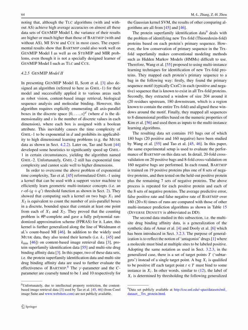
noting that, although the TLC algorithms (with and with-out AS) achieve high average accuracies on almost all thesedata sets of GENMIP Model I, the variance of their resultsare higher or much higher than those of BARTMIP (with andwithout AS), MI SVM and CCE in most cases. The experi-mental results show that BARTMIP could also work well onGENMIP Model I as well as on STDMIP and MIR prob-lems, even though it is not a specially designed learner ofGENMIP Model I such as TLC and CCE.

4.2.5 GENMIP Model II

In presenting GENMIP Model II, Scott et al. [3] also de-signed an algorithm (referred to here as GMIL-1) for theirmodel and successfully applied it to various areas suchas robot vision, content-based image retrieval, biologicalsequence analysis and molecular binding. However, thisalgorithm requires explicitly enumerating all axis-parallelboxes in the discrete space {0, . . . , s}d (where d is the di-mensionality and s is the number of discrete values in eachdimension), where each box is assigned with a booleanattribute. This inevitably causes the time complexity ofGMIL-1 to be exponential in d and prohibits its applicabil-ity to high dimensional learning problems (e.g. the MUSK

data as shown in Sect. 4.2.2). Later on, Tao and Scott [44]developed some heuristics to significantly speed up GMIL-1 in certain circumstances, yielding the algorithm namedGMIL-2. Unfortunately, GMIL-2 still has exponential timecomplexity and cannot scale well to higher dimensions.

In order to overcome the above problem of exponentialtime complexity, Tao et al. [45] reformulated GMIL-1 usinga kernel that can be used with a support vector machine toefficiently learn geometric multi-instance concepts (i.e. anr-of-(q + q ′) threshold function as shown in Sect. 2). Theyshowed that computing such a kernel on two bags X1 andX2 is equivalent to count the number of axis-parallel boxesin a discrete, bounded space that contain at least one pointfrom each of X1 and X2. They proved that the countingproblem is #P-complete and gave a fully polynomial ran-domized approximation scheme (FPRAS) for it. Later, thiskernel is further generalized along the line of Weidmann etal.’s count-based MI [46]. In addition to the widely usedMUSK data, they also tested their kernels (i.e. k∧ [45] andkmin [46]) on content-based image retrieval data [3], pro-tein superfamily identification data [55] and multi-site drugbinding affinity data [3]. In this paper, two of these data sets,i.e. the protein superfamily identification data and multi-sitedrug binding affinity data are used to further evaluate theeffectiveness of BARTMIP.8 The γ -parameter and the C-parameter are coarsely tuned to be 1 and 10 respectively for

8Unfortunately, due to intellectual property restriction, the content-based image retrieval data [3] used by Tao et al. [45, 46] (from Corelimage Suite and www.webshots.com) are not publicly available.

the Gaussian kernel SVM, the results of other comparing al-gorithms are all from [45] and [46].

The protein superfamily identification data9 deals withthe problem of identifying new Trx-fold (Thioredoxin-fold)proteins based on each protein’s primary sequence. How-ever, the low conservation of primary sequence in the Trx-fold superfamily makes conventional modeling methodssuch as Hidden Markov Models (HMMs) difficult to use.Therefore, Wang et al. [55] proposed to using multi-instancelearning techniques for identification of new Trx-fold pro-teins. They mapped each protein’s primary sequence to abag in the following way: firstly, they found the primarysequence motif (typically CxxC) in each (positive and nega-tive) sequence that is known to exist in all Trx-fold proteins.Secondly, they extracted a window of size 204 around it(20 residues upstream, 180 downstream, which is a regionknown to contain the entire Trx-fold) and aligned these win-dows around the motif. Finally, they mapped all sequencesto 8-dimensional profiles based on the numeric properties ofKim et al. [56] and used them as inputs to the multi-instancelearning algorithms.

The resulting data set contains 193 bags out of which180 bags (20 positive and 160 negative) have been studiedby Wang et al. [55] and Tao et al. [45, 46]. In this paper,the same experimental setup is used to evaluate the perfor-mance of BARTMIP on this data set. In detail, 20-fold cross-validation on 20 positive bags and 8-fold cross-validation on160 negative bags are performed. In each round, BARTMIP

is trained on 19 positive proteins plus one of 8 sets of nega-tive proteins, and then tested on the held-out positive proteinplus the remaining 7 sets of negative proteins. The aboveprocess is repeated for each positive protein and each ofthe 8 sets of negative proteins. The average predictive error,false positive rate and false negative rate of BARTMIP over160 (20×8) times of runs are compared with those of othermulti-instance prediction algorithms as shown in Table 15(DIVERSE DENSITY is abbreviated as DD).

The second data studied in this subsection, i.e. the multi-site drug binding affinity data, is a generalization of thesynthetic data of Amar et al. [4] and Dooly et al. [6] whichhas been introduced in Sect. 3.2.3. The purpose of general-ization is to reflect the notion of ‘antagonist’ drugs [1] wherea molecule must bind at multiple sites to be labeled positive.Adopting the same notation as used in Sect. 3.2.3, in thegeneralized case, there is a set of target points T (‘subtar-gets’) instead of a single target point. A bag Xi is qualifiedto be positive iff each target point t ∈ T must bind to someinstance in Xi . In other words, similar to (12), the label ofXi is determined by thresholding the following generalized

9Data set publicly available at http://cse.unl.edu/~qtao/datasets/mil_dataset__Trx_protein.html.

http://www.webshots.com

http://cse.unl.edu/~qtao/datasets/mil_dataset__Trx_protein.html

http://cse.unl.edu/~qtao/datasets/mil_dataset__Trx_protein.html


Table 15 Performance of eachcomparing algorithm on theprotein superfamilyidentification data in terms ofpredictive error, false positiverate and false negative rate

Evaluation criterion BARTMIP k∧ kmin GMIL-1 GMIL-2 EMDD DD

PREDICTIVE ERROR 0.235 0.218 0.215 N/A 0.250 0.365 0.664

FALSE POSITIVE RATE 0.235 0.218 0.215 N/A 0.250 0.365 0.668

FALSE NEGATIVE RATE 0.244 0.169 0.144 N/A 0.250 0.360 0.125

Table 16 Predictive error ofeach comparing algorithm onthe multi-site drug bindingaffinity data

Data set BARTMIP k∧ kmin GMIL-1 GMIL-2 EMDD DD

5-dim 0.190 0.205 N/A 0.212 0.218 0.191 0.196

10-dim 0.178 0.175 N/A N/A N/A 0.223 0.216

20-dim 0.195 0.207 N/A N/A N/A 0.268 0.255

real-valued label GRLXiat 1/2:

GRLXi= min

t∈T

{

maxXij ∈Xi

{∑nk=1 sk · V (tk − Xijk)

Emax

}}

(13)

Using the above generalized data generator, Scott etal. [3] build ten 5-dimensional data sets (200 training bagsand 200 testing bags) each with 4 subtargets and tested theiralgorithm GMIL-1 on them. Tao et al. [45] also generateddata with dimension 10 and 20, each with 5 subtargets, tofurther evaluate how well their algorithm k∧ handles higher-dimensional data. As with the 5-dimensional data, ten setswere generated, each containing 200 training bags and 200testing bags. The average predictive errors of BARTMIP

on these data sets (with dimensionality of 5, 10 and 20)are compared with those of other multi-instance learningalgorithms as shown Table 16 (DIVERSE DENSITY is ab-breviated as DD).

On the protein superfamily identification data (as shownin Table 15), in terms of all evaluation criteria, the perfor-mance of BARTMIP is worse than those of k∧ and kmin,but significantly better than those of GMIL-2 and EMDD.Furthermore, DIVERSE DENSITY significantly outperformsall the other comparing algorithms in terms of false neg-ative rate. On the multi-site drug binding affinity data (asshown in Table 16), the performance of BARTMIP is compa-rable, and in most cases superior to the those of k∧, GMIL-1,GMIL-2, EMDD and DIVERSE DENSITY. These experimen-tal results show that BARTMIP could also work well onGENMIP Model II as well as on STDMIP and MIR prob-lems, even though it is not a specially designed learner ofGENMIP Model II such as GMIL-1, GMIL-2, k∧ and kmin.

5 Discussion

As mentioned in Sect. 4.1, BARTMIP solves multi-instanceprediction problems by transforming the representation tomeet the requirement of traditional supervised learning al-gorithms. Actually, several algorithms, especially those for

GENMIP problems, such as TLC [2], CCE [43], GMIL-1[3], GMIL-2 [44], k∧ [45] and kmin [46] have also beendesigned along this way. In this section, the relationships be-tween BARTMIP and those algorithms are discussed in moredetail.

Weidmann et al. [2] proposed TLC to tackle GENMIPModel I problems, which constructs a meta-instance foreach bag and then passes the meta-instance and the classlabel of the corresponding bag to a common classifier. TLC

uses a standard decision tree for imposing a structure on theinstance space, which is trained on the set of all instancescontained in all bags where the instances are labeled withtheir bag’s class label, so that a meta-instance is generatedfor each bag. However, simply labeling the instances withtheir bag’s class label for decision tree building may be mis-leading. For instance, in STDMIP problems (special case ofpresence-based MI problems with |C| = 1), not all the in-stances in a positive bag should also be labeled positive. Incontrast to TLC, BARTMIP performs unsupervised cluster-ing at the level of bags for representation transformation,where the label of each bag is not necessarily shared by itsinstances.

Scott et al. [3] proposed GMIL-1 to tackle GENMIPModel II problems, which operates in a discretized featurespace X = {0, . . . , s}d (as shown in Sect. 4.2.5). GMIL-1works by enumerating the set of all possible axis-parallelboxes BX (including degenerate ones) in X (so that |BX | =((s+1

2 ) + (s + 1))d = (s+22 )d ), and then creating two boolean

attributes ab and ab (ab = 1 − ab) for each box b ∈ BX .Given a bag X = (x1, . . . , xp), the algorithm set ab = 1 ifsome point from X lies in b and ab = 0 otherwise. Us-ing the above remapping of each bag to 2|BX | booleanattributes, the target concept defined by some C, C and r

(as shown in Sect. 2) can be represented by an r-of-(q + q ′)threshold function over the attributes aci

for ci ∈ C andacj

for cj ∈ C. As shown in [3], such a threshold func-tion can be easily learned by WINNOW [57] while makingonly O(r(q + q ′)d log s) mistakes in an online learningsetting. Unfortunately, the time complexity of GMIL-1 is


exponential in both log s and d . Although Tao and Scott[44] have developed some heuristics (GMIL-2) to signif-icantly improve the computation efficiency of GMIL-1 incertain situations, GMIL-2 still has exponential time com-plexity which limits its application to problems with higherdimensions. In contrast to GMIL-1 and GMIL-2, BARTMIP

could scale quite well to learning problems with higher di-mensions, such as those problems shown in Sects. 4.2.2and 4.2.3.

For those algorithms mentioned above, i.e. TLC [2],GMIL-1 [3] and GMIL-2 [44], together with k∧ [45] andkmin [46] (kernel reformulations of GMIL-1), bags are trans-formed into corresponding feature vectors in a supervisedway. That is, the boolean label of each bag is essential for theprocess of representation transformation. While for BART-MIP, this process is accomplished in an unsupervised way byunsupervised clustering at the level of bags. One advantageof unsupervised clustering is that BARTMIP could be eas-ily adapted to solve MIR problems with real-valued outputs,which is much more difficult for TLC, GMIL-1, GMIL-2, k∧and kmin to do so. Another advantage of unsupervised clus-tering is that additional unlabeled bags, if available, could beincorporated with the labeled training bags in the clusteringprocess. For instance, in the problem of content-based imageretrieval using multi-instance learning techniques [36, 37],only a few images (bags) will be labeled by the users whileplenty of unlabeled images are available in the databasewhich could be combined with the labeled ones to get morereliable clustering results.

CCE [43] also performs representation transformation inan unsupervised way. Firstly, all the instances contained inall the bags are collected, and the popular clustering algo-rithm k-MEANS [58] is employed to cluster the instancesinto d groups. Secondly, each bag is transformed into ad-dimensional feature vector, where if the bag has some in-stances being clustered to the i-th group, then the value ofthe i-th feature is set to 1 and 0 otherwise. They also usesupport vector machines to build a classifier on the trans-formed feature vectors. Finally, considering that there is nocriterion available for judging which kind of clustering re-sult is the best for re-representation of the bags, the aboveprocedures are repeated with different values of d where anensemble of m classifiers are produced and their outputs arecombined by majority voting when making predictions forunseen bags. Although in this way CCE could utilize thepower of ensemble learning [59] to achieve strong gener-alization ability, experimental results reported in Sect. 4.2.4show that its generalization ability is still worse than thatof BARTMIP, which is only a single multi-instance learner.The superiority of BARTMIP may attribute to the clusteringresults obtained by BAMIC which successfully reveal the un-derlying distribution of training bags.

As already mentioned several times, a unique character-istic of BARTMIP is that it performs representation transfor-mation by structuring the input space at the level of bagsinstead of at the level of instances. Specifically, TLC [2]structures the input space by building a decision tree fromthe set of all instances contained in all bags by sharingthe bag’s class label to its component instances; GMIL-1[3], GMIL-2 [44], k∧ [45] and kmin [46] structures theinput space by enumerating all the axis-parallel boxes at in-stance level and then constructing boolean attributes fromthose boxes; CCE [43] structures the input space by dividingthe instances into many disjoint regions using the populark-MEANS clustering algorithm. However, BARTMIP struc-tures the input space at the level of bags by clustering thetraining bags into several disjoint groups of bags. We sup-pose that this kind of representation transformation strategyis more pertinent to the original representation of multi-instance learning, i.e. each object represented by a bag (a setof feature vectors) instead of one feature vector.

6 Conclusion

In this paper, the problem of unsupervised multi-instancelearning is addressed where a novel multi-instance cluster-ing algorithm named BAMIC is proposed. BAMIC seeks tocluster training bags into a number of disjoint groups ofbags, where the popular k-MEDOIDS algorithm is adaptedby using some form of distance metric to measure distancebetween bags. Based on the information provided by theclustering results of BAMIC, a novel multi-instance pre-diction algorithm named BARTMIP is proposed. BARTMIP

re-represents each bag by a feature vector whose featurevalues are set to be the distances between the bag andthe medoids of clustered groups. Therefore, the bags aretransformed into feature vectors so that common supervisedlearners (support vector machines in this paper) are used tolearn from the induced data set. Extensive experiments showthat BAMIC could effectively reveal the underlying structureof multi-instance data sets while BARTMIP is highly com-parable to other multi-instance prediction algorithms on awide range of multi-instance prediction problems, includingSTDMIP, MIR and two kinds of GENMIP models.

BAMIC is the first work toward unsupervised multi-instance learning, it is obvious that investigating other kindsof unsupervised multi-instance learning methods to yieldbetter learning ability is an important and interesting issueworth further study.

For BAMIC, there will exist some clusters containingonly one bag when the number of clustered groups is large.Investigating some appropriate methods to eliminate these‘trivial’ clusters is an important issue for future work. Fur-ther evaluating the performance of BARTMIP on more avail-able multi-instance data sets will be another interestingfuture work.


In addition to several well-established algorithms [2, 3,43–46], the success of BARTMIP further shows the feasi-bility of solving multi-instance prediction problems throughrepresentation transformation. Actually, there are many pos-sible ways for this purpose. For examples, referring to Fig. 6,each bag can be transformed into a feature vector whosei-th feature equals the average distance of it to all the bagsin Gi instead of the distance of it to the medoid of Gi .Furthermore, besides support vector machines, other super-vised learning methods such as neural networks can also beused as the classifier training algorithms. Exploring otherschemes for modifying the representation of multi-instanceprediction problems is also an interesting issue for futurework.

Acknowledgements The authors wish to thank the anonymous re-viewers for their helpful comments and suggestions. The authors alsowish to thank N. Weidmann for the artificial data sets of GENMIPModel I, T. Osugi for the code of k∧, Q. Tao for the multi-site drugbinding affinity data, and S. D. Scott and S. A. Goldman for their kindhelp. This work was supported by the National Science Foundation ofChina (60635030, 60721002), the National High Technology Researchand Development Program of China (2007AA01Z169), and the StartupFoundation for Excellent New Faculties of Hohai University.

References

1. Dietterich TG, Lathrop RH, Lozano-Pérez T (1997) Solving themultiple-instance problem with axis-parallel rectangles. Artif In-tell 39(1-2):31–71

2. Weidmann N, Frank E, Pfahringer B (2003) A two-level learn-ing method for generalized multi-instance problem. In: Lavrac N,Gamberger D, Blockeel H, Todorovski L (eds) Lecture notes inartificial intelligence, vol 2837. Springer, Berlin, pp 468–579

3. Scott S, Zhang J, Brown J (2003) On generalized multiple-instance learning. Technical report UNL-CSE-2003-5, Depart-ment of Computer Science and Engineering, University of Ne-braska, Lincoln, NE

4. Amar RA, Dooly DR, Goldman SA, Zhang Q (2001) Multiple-instance learning of real-valued data. In: Proceedings of the 18thinternational conference on machine learning, Williamstown, MA,2001, pp 3–10

5. Ray S, Page D (2001) Multiple instance regression. In: Proceed-ings of the 18th international conference on machine learning,Williamstown, MA, 2001, pp 425–432

6. Dooly DR, Zhang Q, Goldman SA, Amar RA (2002) Multiple-instance learning of real-valued data. J Mach Learn Res 3:651–678

7. Han J, Kamber M (2001) Data mining: concepts and techniques.Morgan Kaufmann, San Francisco

8. Edgar GA (1995) Measure, Topology, and Fractal Geometry, 3rdedn. Springer, Berlin

9. Long PM, Tan L (1998) PAC learning axis-aligned rectangles withrespect to product distribution from multiple-instance examples.Mach Learn 20(1):7–21

10. Auer P, Long PM, Srinivasan A (1998) Approximating hyper-rectangles: learning and pseudo-random sets. J Comput Syst Sci57(3):376–388

11. Auer P (1997) On learning from multi-instance examples: empir-ical evaluation of a theoretical approach. In: Proceedings of the14th international conference on machine learning, Nashville, TN,1997, pp 21–29

12. Blum A, Kalai A (1998) A note on learning from multiple-instanceexamples. Mach Learn 30(1):23–29

13. Goldman SA, Kwek SS, Scott SD (2001) Agnostic learning ofgeometric patterns. J Comput Syst Sci 62(1):123–151

14. Goldman SA, Scott SD (2003) Multiple-instance learning of real-valued geometric patterns. Ann Math Artif Intell 39(3):259–290

15. Maron O, Lozano-Pérez T (1998) A framework for multiple-instance learning. In: Jordan MI, Kearns MJ, Solla SA (eds)Advances in neural information processing systems, vol 10. MITPress, Cambridge, pp 570–576

16. Zhang Q, Goldman SA (2002) EM-DD: an improved multiple-instance learning technique. In: Dietterich TG, Becker S, Ghahra-mani Z (eds) Advances in neural information processing systems,vol 14. MIT Press, Cambridge, pp 1073–1080

17. Chen Y, Wang JZ (2004) Image categorization by learning andreasoning with regions. J Mach Learn Res 5:913–939

18. Wang J, Zucker J-D (2000) Solving the multiple-instance prob-lem: a lazy learning approach. In: Proceedings of the 17th interna-tional conference on machine learning, San Francisco, CA, 2000,pp 1119–1125

19. Ruffo G (2000) Learning single and multiple decision trees forsecurity applications. Ph.D. thesis, Department of Computer Sci-ence, University of Turin, Italy, 2000

20. Chevaleyre Y, Zucker J-D (2001) Solving multiple-instance andmultiple-part learning problems with decision trees and decisionrules. Application to the mutagenesis problem. In: Stroulia E,Matwin S (eds) Lecture notes in artificial intelligence, vol 2056.Springer, Berlin, pp 204–214

21. Blockeel H, Page D, Srinivasan A (2005) Multi-instance treelearning. In: Proceedings of the 22nd international conference onmachine learning, Bonn, Germany, 2005, pp 57–64

22. Xu X, Frank E (2004) Logistic regression and boosting for labeledbags of instances. In: Dai H, Srikant R, Zhang C-Q (eds) Lecturenotes in computer science, vol 3056. Springer, Berlin, pp 272–281

23. Ramon J, De Raedt L (2000) Multi instance neural networks. In:Proceedings of ICML-2000, workshop on attribute-value and re-lational learning, San Francisco, CA, 2000

24. Zhou Z-H, Zhang M-L (2002) Neural networks for multi-instancelearning. Technical report, AI Lab, Computer Science and Tech-nology Department, Nanjing University, Nanjing, China

25. Zhang M-L, Zhou Z-H (2004) Improve multi-instance neural net-works through feature selection. Neural Process Lett 19(1):1–10

26. Bouchachia A (2004) Multiple instance learning with radial basisfunction neural networks. In: Pal NR, Kasabov N, Mudi RK (eds)Lecture notes in computer science, vol 3316. Springer, Berlin, pp440–445

27. Zhang M-L, Zhou Z-H (2006) Adapting RBF neural networks tomulti-instance learning. Neural Process Lett 23(1):1–26

28. Gärtner T, Flach PA, Kowalczyk A, Smola AJ (2002) Multi-instance kernels. In: Proceedings of the 19th international confer-ence on machine learning, Sydney, Australia, 2002, pp 179–186

29. Andrews S, Tsochantaridis I, Hofmann T (2003) Support vectormachines for multiple-instance learning. In: Becker S, Thrun S,Obermayer K (eds) Advances in neural information processingsystems, vol 15. MIT Press, Cambridge, pp 561–568

30. Cheung P-M, Kwok JT (2006) A regularization framework formultiple-instance learning. In: Proceedings of the 23th interna-tional conference on machine learning, Pittsburgh, PE, 2006, pp193–200

31. Zhou Z-H, Zhang M-L (2003) Ensembles of multi-instance learn-ers. In: Lavrac N, Gamberger D, Blockeel H, Todorovski L (eds)Lecture notes in artificial intelligence, vol 2837. Springer, Berlin,pp 492–502

32. Andrews S, Hofmann T (2004) Multiple-instance learning via dis-junctive programming boosting. In: Thrun S, Saul LK, SchölkopfB (eds) Advances in neural information processing systems, vol16. MIT Press, Cambridge


33. Auer P, Ortner R (2004) A boosting approach to multiple instancelearning. In: Boulicaut J-F, Esposito F, Giannotti F, Pedreschi D(eds) Lecture notes in artificial intelligence, vol 3201. Springer,Berlin, pp 63–74

34. Viola P, Platt J, Zhang C (2006) Multiple instance boosting for ob-ject detection. In: Weiss Y, Schölkopf B, Platt J (eds) Advances inneural information processing systems, vol 18. MIT Press, Cam-bridge, pp 1419–1426

35. Huang X, Chen S-C, Shyu M-L, Zhang C (2002) Mining high-level user concepts with multiple instance learning and relevancefeedback for content-based image retrieval. In: Zaïane OR, SimoffSJ, Djeraba C (eds) Lecture notes in artificial intelligence, vol2797. Springer, Berlin, pp 50–67

36. Yang C, Lozano-Pérez T (2000) Image database retrieval withmultiple-instance learning techniques. In: Proceedings of the 16thinternational conference on data engineering, San Diego, CA,2000, pp 233–243

37. Zhang Q, Yu W, Goldman SA, Fritts JE (2002) Content-based im-age retrieval using multiple-instance learning. In: Proceedings ofthe 19th international conference on machine learning, Sydney,Australia, 2002, pp 682–689

38. Zhou Z-H, Zhang M-L, Chen K-J (2003) A novel bag generator forimage database retrieval with multi-instance learning techniques.In: Proceedings of the 15th IEEE international conference on toolswith artificial intelligence, Sacramento, CA, 2003, pp 565–569

39. Rahmani R, Goldman SA (2006) Missl: multiple-instance semi-supervised learning. In: Proceedings of the 23rd internationalconference on machine learning, Pittsburgh, PE, 2006, pp 705–712

40. Maron O, Ratan AL (1998) Multiple-instance learning for naturalscene classification. In: Proceedings of the 15th international con-ference on machine learning, Madison, WI, 1998, pp 341–349

41. McGovern A, Barto AG (2001) Automatic discovery of subgoalsin reinforcement learning using diverse density. In: Proceed-ings of the 18th international conference on machine learning,Williamstown, MA, 2001, pp 361–368

42. Zhou Z-H, Jiang K, Li M (2005) Multi-instance learning basedweb mining. Appl Intell 22(2):135–147

43. Zhou Z-H, Zhang M-L (2007) Solving multi-instance problemswith classifier ensemble based on constructive clustering. KnowlInf Syst 11(2):155–170

44. Tao Q, Scott S (2004) A faster algorithm for generalized multiple-instance learning. In: Proceedings of the 17th international Floridaartificial intelligence research society conference, Miami Beach,FL, 2004, pp 550–555

45. Tao Q, Scott S, Vinodchandran NV, Osugi TT (2004) Svm-based generalized multiple-instance learning via approximate boxcounting. In: Proceedings of the 21st international conference onmachine learning, Banff, Canada, 2004, pp 799–806

46. Tao Q, Scott S, Vinodchandran NV, Osugi TT, Mueller B (2004)An extended kernel for generalized multiple-instance learning. In:Proceedings of the 16th IEEE international conference on toolswith artificial intelligence, Boca Raton, FL, 2004, pp 272–277

47. De Raedt L (1998) Attribute-value learning versus inductive logicprogramming: the missing links. In: Page D (ed) Lecture notes inartificial intelligence, vol 1446. Springer, Berlin, pp 1–8

48. Alphonse É, Matwin S (2004) Filtering multi-instance problemsto reduce dimensionality in relational learning. J Intell Inf Syst22(1):23–40

49. McGovern A, Jensen D (2003) Identifying predictive structures inrelational data using multiple instance learning. In: Proceedings ofthe 20th international conference on machine learning, Washing-ton, DC, 2003, pp 528–535

50. Günter S, Bunke H (2003) Validation indices for graph clustering.Pattern Recogn Lett 24(8):1107–1113

51. Quinlan JR (1993) C4.5: Programs for machine learning. MorganKaufmann, San Mateo

52. Blake C, Keogh E, Merz CJ (1998) UCI repository of machinelearning databases [http://www.ics.uci.edu/~mlearn/mlrepository.html]. Technical report, Department of Information and ComputerScience, University of California, Irvine, CA

53. Berry RS, Rice SA, Ross J (1980) Physical Chemistry. Wiley, NewYork, Chapter 10, Intermolecular Forces

54. Liu H, Motoda H (1998) Feature selection for knowledge discov-ery and data mining. Kluwer Academic, Norwell

55. Wang C, Scott SD, Zhang J, Tao Q, Fomenko D, GladyshevV (2004) A study in modeling low-conservation protein super-families. Technical report UNL-CSE-2004-0003, Department ofComputer Science and Engineering, University of Nebraska, Lin-coln, NE

56. Kim J, Moriyama EN, Warr CG, Clyne PJ, Carlson JR (2000)Identification of novel multi-transmembrane proteins from ge-nomic databases using quasi-periodic structural properties. Bioin-form 16(9):767–775

57. Littlestone N (1991) Redundant noisy attributes, attribute errors,and linear threshold learning using winnow. In: Proceedings ofthe 4th annual workshop on computational learning theory, SantaCruz, CA, 1991, pp 147–156

58. Bishop CM (1995) Neural networks for pattern recognition. Ox-ford University Press, New York

59. Dietterich TG (2000) Ensemble methods in machine learning. In:Kittler J, Roli F (eds) Lecture notes in computer science, vol 1867.Springer, Berlin, pp 1–15

60. Chang C-C, Lin C-J (2001) LIBSVM: a library for support vec-tor machines. Technical report, Department of Computer Scienceand Information Engineering, National Taiwan University, Taipei,Taiwan

61. Ray S, Craven M (2005) Supervised versus multiple instancelearning: an empirical comparison. In: Proceedings of the 22ndinternational conference on machine learning, Bonn, Germany,2005, pp 697–704

62. Tan X, Chen S, Zhou Z-H, Liu J (2006) Learning non-metric par-tial similarity based on maximal margin criterion. In: Proceedingsof the IEEE computer society conference on computer vision andpattern recognition, New York, NY, 2006, pp 138–145

http://www.ics.uci.edu/~mlearn/mlrepository.html

http://www.ics.uci.edu/~mlearn/mlrepository.html

Documents

Multi-instance clustering with applications to multi-instance prediction