Multi-Hypergraph Learning for Incomplete Multimodality Data

IEEE JOURNAL OF BIOMEDICAL AND HEALTH INFORMATICS, VOL. 22, NO. 4, JULY 2018 1197

Multi-Hypergraph Learning for IncompleteMultimodality Data

Mingxia Liu , Member, IEEE, Yue Gao , Senior Member, IEEE, Pew-Thian Yap, Senior Member, IEEE,and Dinggang Shen , Senior Member, IEEE

Abstract—Multi-modality data convey complementaryinformation that can be used to improve the accuracy ofprediction models in disease diagnosis. However, effec-tively integrating multi-modality data remains a challeng-ing problem, especially when the data are incomplete. Forinstance, more than half of the subjects in the Alzheimer’sdisease neuroimaging initiative (ADNI) database have nofluorodeoxyglucose positron emission tomography andcerebrospinal fluid data. Currently, there are two commonlyused strategies to handle the problem of incomplete data:1) discard samples having missing features; and 2) im-pute those missing values via specific techniques. In thefirst case, a significant amount of useful information islost and, in the second case, additional noise and artifactsmight be introduced into the data. Also, previous studiesgenerally focus on the pairwise relationships among sub-jects, without considering their underlying complex (e.g.,high-order) relationships. To address these issues, in thispaper, we propose a multi-hypergraph learning method fordealing with incomplete multimodality data. Specifically, wefirst construct multiple hypergraphs to represent the high-order relationships among subjects by dividing them intoseveral groups according to the availability of their datamodalities. A hypergraph regularized transductive learn-ing method is then applied to these groups for automaticdiagnosis of brain diseases. Extensive evaluation of theproposed method using all subjects in the baseline ADNIdatabase indicates that our method achieves promising re-sults in AD/MCI classification, compared with the state-of-the-art methods.

Index Terms—Alzheimer’s disease, classification, hyper-graph, incomplete data, multi-modality.

I. INTRODUCTION

Alzheimer’s disease (AD) is characterized by progressiveimpairment of neurons and the connections between neurons,leading to loss of cognitive/memory function and ultimately

Manuscript received January 14, 2017; revised June 23, 2017; ac-cepted July 24, 2017. Date of publication July 25, 2017; date of cur-rent version June 29, 2018. This work was supported by the NationalInstitutes of Health under Grants EB006733, EB008374, EB009634,MH100217, AG041721, AG042599, AG010129, and AG030514. (Corre-sponding author: Dinggang Shen.)

M. Liu, Y. Gao, and P.-T. Yap are with the Department of Radiol-ogy and BRIC, University of North Carolina at Chapel Hill, Chapel Hill,NC 27599 USA (e-mail: [email protected]; [email protected]; [email protected]).

D. Shen is with the Department of Radiology and BRIC, University ofNorth Carolina at Chapel Hill, Chapel Hill, NC 27599 USA and also withthe Department of Brain and Cognitive Engineering, Korea University,Seoul 02841, South Korea (e-mail: [email protected]).

Digital Object Identifier 10.1109/JBHI.2017.2732287

death. This disease has been regarded as the major challenge toglobal health care systems [1], and it is estimated that the totalprevalence of AD in the United States is about 13.8 million by2050 [2]. Until now, much effort has been made to investigatecomputer-aided brain disease diagnosis approaches, aiming toprevent or postpone the onset of AD or its prodrome, i.e., mildcognitive impairment (MCI) [3].

Recent research and clinical studies have investi-gated extensive candidate biomarkers, and reported thatfluorodeoxyglucose positron emission tomography (PET) mea-surements, structural magnetic resonance imaging (MRI), andcerebrospinal fluid (CSF) are among the best-establishedbiomarkers for AD progression and pathology [3]. Specifically,feature representations (e.g., cortical thickness, connectivity in-formation, and regional volumetric measures) extracted fromMRI can be adopted to measure AD-related brain abnormali-ties [4]–[11]. With PET data, one can detect the abnormalityin cerebral metabolic rate for glucose in the brain [12]–[16].Besides, CSF total-tau (t-tau), CSF tau hyperphosphorylated atthreonine 181 (p-tau) and the decrease of CSF amyloid β (Aβ)are shown to be related to the cognitive decline in AD/MCIpatients [17], [18]. Previous computer-aided disease diagno-sis studies have reported that multi-modality data (e.g., MRI,PET, and CSF) can provide complementary information [19]–[22], which can be used for improving the diagnostic results forAD/MCI.

One common challenge in the multi-modality analysis isthat there may be missing values in some modalities, whichis called incomplete data problem [19], [20]. For instance, theAlzheimer’s Disease Neuroimaging Initiative (ADNI) database,which consists of data for AD, MCI, and normal control (NC)subjects with multiple data modalities (e.g., MRI, PET, andCSF), is not complete for all modalities [23]. In the baselineADNI database, all subjects have MRI data, and only about halfsubjects have PET and CSF data. Possible reasons for this mayinclude poor data quality, high cost involved with PET scanningand patient dropouts. For instance, CSF data collection requiresinvasive tests (e.g., lumbar puncture), which might deter patientcommitment [19].

In the domain of neuroimaging analysis, researchers have de-veloped various approaches to deal with incomplete data [19],[20]. The first type of methods simply removes subjects withincomplete data. This will unfortunately result in discardinga large amount of the acquired data and may lead to signifi-cant reduction of sample size [24]. The second type of methods

2168-2194 © 2017 IEEE. Personal use is permitted, but republication/redistribution requires IEEE permission.See http://www.ieee.org/publications standards/publications/rights/index.html for more information.

https://orcid.org/0000-0002-0598-5692

https://orcid.org/0000-0002-4971-590X

https://orcid.org/0000-0002-7934-5698

1198 IEEE JOURNAL OF BIOMEDICAL AND HEALTH INFORMATICS, VOL. 22, NO. 4, JULY 2018

aims to impute the missing values via specific data imputationtechniques [25], [26]. Some well-known imputation techniquesinclude expectation maximization (EM) [27], singular value de-composition (SVD) [28] and matrix completion [29]. Althoughthese methods may help to process those randomly missing data,they often cannot handle missing data that are in a block-wisemanner [19], where subjects have missing values in a wholemodality (instead of missing some features in a specific modal-ity). Also, imputation methods may introduce additional im-putation artifacts, and thus, degrade the data quality [29]. Dif-ferent from these two categories, several other methods havebeen recently developed to directly handle the incomplete data,without having to discard incomplete data or to impute missingdata [19], [20]. For instance, Yuan et al. [19] proposed a multi-source feature learning method using all subjects in ADNI withat least one available data modality. Xiang et al. [20] devel-oped a sparse feature learning method for handling incompletemulti-modality data without imputation. However, the main dis-advantage of these methods is that they model only the pairwiserelationships between subjects. Intuitively, the higher-order re-lationships among subjects can be used to improve the learningperformance of computer-aided AD/MCI diagnosis.

In this paper, we propose a multi-hypergraph learning (MHL)approach based on incomplete multi-modality data for the au-tomatic diagnosis of AD/MCI, where the high-order relation-ships among subjects can be modeled explicitly. To be specific,we first divide the dataset into several groups depending onwhether the data for a certain modality is available. In this way,each group contains subjects with complete data from a partic-ular combination of different modalities. Then, we construct ahypergraph to model the high-order relationships among sub-jects in each group. Next, we combine the hyperedges given bymulti-hypergraphs associated with those groups and compute ahypergraph Laplacian matrix. Finally, a hypergraph-regularizedtransductive learning model is used for AD/MCI diagnosis.

The major contributions of this paper are summarized below.First, we propose a data grouping strategy for multi-modalitydata, and each group is corresponding to a particular com-bination of multiple modalities. Second, we develop a multi-hypergraph classification model, by explicitly modeling the in-herent high-order relationships among subjects via hypergraphs.Third, we conduct extensive experiments on ADNI to empiri-cally analyze our method, including four binary classificationtasks (i.e., AD vs. NC, MCI vs. NC, AD vs. MCI, and pMCI vs.sMCI). The experimental results demonstrate the effectivenessof our proposed method.

The work in this paper is different from our previous studyin [30]. First, while the focus of [30] is to exploit the coherenceamong different data groups (with each group containing datafrom a particular combination of different modalities), we fo-cus on modeling the high-order relationships among subjects inthis study. Second, the strategies for making use of the multi-modality data are different. In [30], we learn optimal weightsfor different groups from data via a view-aligned hypergraphclassification model. In this work, we treat each group equallyand propose to learn weights for hyperedges from data automati-cally. Third, the hypergraph construction methods are different.

In [30], we adopt sparse representation for constructing hy-pergraphs, where the similarity measure is based on the sparsecoefficients. In this work, we use the star expansion strategy [31]to generate multiple hyperedges in each group, where Euclideandistance is used as the similarity measure.

The rest of the paper is organized as follows. We first presentbackground information in Section II. In Section III, we describedata pre-processing method and our proposed multi-hypergraphlearning approach. In Section IV, we describe experimental set-tings and report experimental results. In Section V, we compareour method with related approaches and investigate the influ-ences of parameters. In Section VI, we conclude this work anddiscuss future research directions.

II. BACKGROUND

A. Hypergraph Based Transductive Learning

As a typical semi-supervised learning method, transductivelearning incorporates not only labeled data but also unlabeleddata for improving the performance of supervised learning meth-ods [32], [33]. Generally, transductive learning assumes thatthe data lie in manifolds and clusters. Based on these two as-sumptions, many transductive learning methods have been pro-posed, such as transductive support vector machine [32], graphbased learning [34], [35] and hypergraph learning [34], [36]–[38]. Among various transductive learning methods, hypergraphlearning achieves promising performance in practice. Here, wedenote scalars, vectors, and matrices using normal italic letters,boldface lowercase letters, and boldface uppercase letters, re-spectively. We further list important notations and definitionsused in this paper in Table I.

A hypergraph is represented by G = (V, E ,w), where V is aset of vertices (each representing a subject), E is a set of hyper-edges (each connecting two or more vertices) and w = (wi) ∈RNe is the weight vector for Ne hyeredges. Each hyperedge ei

(i = 1, 2, · · · , Ne) is assigned a weight wi . In hypergraphs, ahyperedge can connect more than two vertices, through whichhigh-order relationships can be modeled explicitly [34], [36]. Incomparison, each edge in a simple graph connects only two ver-tices. The incidence matrix H = (hij ) ∈ RN ×Ne of hypergraphG encodes the relationships among vertices. The (i, j)-entry ofthe incidence matrix H indicates whether vertex vi is connectedwith other vertices in the hyperedge ej , i.e.,

hij =

{1, if vi ∈ ej

0, otherwise(1)

The vertex degree and the hyperedge degree are defined,respectively, as

d (vi) =∑ej ∈E

wjhij (2)

and

δ(ej ) =∑vi ∈V

hij (3)

We let Dv and De be diagonal matrices containingthe vertex degrees and the hyperedge degrees, respectively.

LIU et al.: MULTI-HYPERGRAPH LEARNING FOR INCOMPLETE MULTIMODALITY DATA 1199

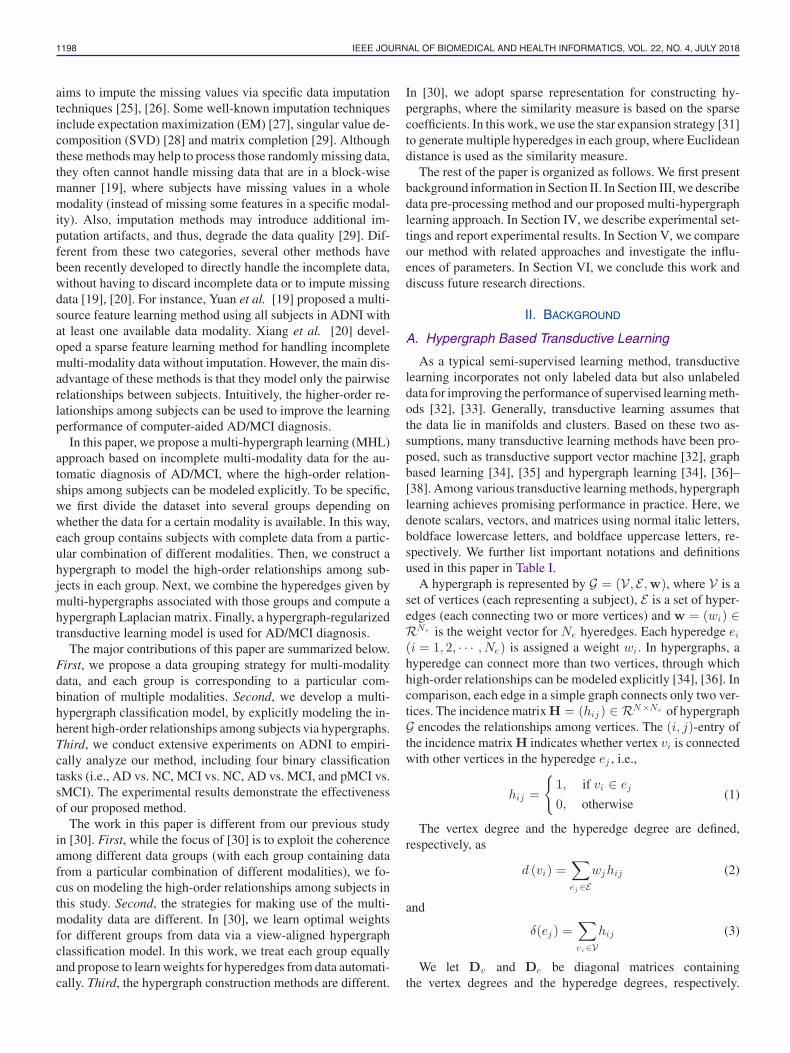
TABLE INOTATIONS

Notation Definition

G = (V, E , w) G denotes a hypergraph, while V , E and w represent the set of vertices, the set of hyperedges and the weights of hyperedges,respectively.

N The number of vertices in the hypergraph G, i.e., N = |V|.Ne The total number of hyperedges, i.e., Ne = |E|.N g

e The number of hyperedges in the g-th group.W The diagonal matrix of the hyperedge weights, W ∈ RN e ×N e .d(vi ) The degree of the vertex vi .δ(ej ) The degree of the hyperedge ej .Dv The diagonal matrix of the vertex degrees, Dv ∈ RN ×N .De The diagonal matrix of the hyperedge degrees, De ∈ RN e ×N e .Hg The incidence matrix for the hypergraph in the g-th group, and Hg ∈ RN ×N e .y The N -dimensional label vector of N samples, with element yi = 1 if the i-th sample belongs to the positive class, yi = −1 if the i-th

sample belongs to the negative class, and otherwise yi = 0.f The relevance score vector for N samples, f ∈ RN .

Denote W = (Wij ) ∈ RNe ×Ne as the diagonal matrix of hy-peredge weights, with the diagonal element Wii = 1. Previ-ous approaches for computing the hypergraph Laplacian canbe categorized into two classes [34]. The first class aims toconstruct a simple graph from the initial hypergraph, e.g., starexpansion [31], clique expansion [31] and Rodriquez’s Lapla-cian [39]. In the second class, we define a hypergraph Laplacianbased on analogs from simple graph Laplacian, e.g., normal-ized Laplacian [34] and Bolla’s Laplacian [40]. Recently, Ben-son et al. [38] proposed a hypergraph construction methodto capture the high-level information inside a graph. In thispaper, we adopt the method proposed in [34] to compute the hy-pergraph Laplacian. Letting Θ = D−1/2

v HWD−1e HTD−1/2

v ,the hypergraph Laplacian is defined as Ł = I − Θ. Wedefine the hypergraph Laplacian regularizer Ω(f) asin [34]

Ω(f) = fTŁf

=12

∑ei ∈E

∑vj ,vk ∈V

wihjihki

δ(ei)

(fj√d(vj )

− fk√d(vk )

)2

(4)

B. ADNI Database

This study is based on the incomplete multi-modality datafrom the baseline ADNI database (ADNI-1) [23]. In ADNI,subjects are divided into three categories (i.e., AD, MCI, andNC) based on particular criteria such as Mini-Mental State Ex-amination (MMSE) scores. To be specific, general inclusionor exclusion criteria used in ADNI are listed in the following:1) mild AD: MMSE scores between 20–26 (inclusive), CDR of0.5 or 1.0 and meet NINCDS/ADRDA criteria for probable AD;2) MCI: MMSE scores between 24–30 (inclusive), a memorycomplaint, have objective memory loss measured by educationadjusted scores on Wechsler Memory Scale Logical MemoryII, a CDR of 0.5, absence of significant levels of impairment inother cognitive domains, essentially preserved activities of dailyliving and an absence of dementia; and 3) NC: Mini-MentalState Examination (MMSE) scores between 24–30 (inclusive),

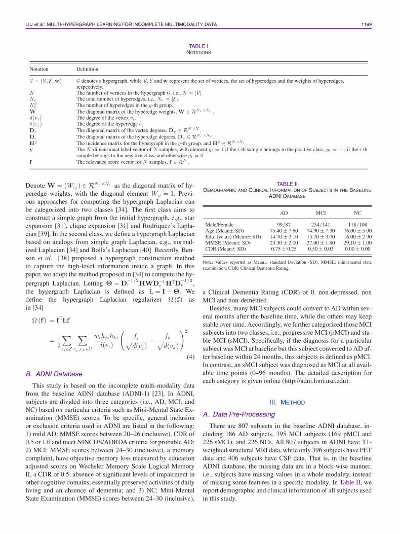
TABLE IIDEMOGRAPHIC AND CLINICAL INFORMATION OF SUBJECTS IN THE BASELINE

ADNI DATABASE

AD MCI NC

Male/Female 99/87 254/141 118/108Age (Mean± SD) 75.40 ± 7.60 74.90 ± 7.30 76.00 ± 5.00Edu. (years) (Mean± SD) 14.70 ± 3.10 15.70 ± 3.00 16.00 ± 2.90MMSE (Mean± SD) 23.30 ± 2.00 27.00 ± 1.80 29.10 ± 1.00CDR (Mean± SD) 0.75 ± 0.25 0.50 ± 0.03 0.00 ± 0.00

Note: Values reported as Mean± standard Deviation (SD); MMSE: mini-mental stateexamination; CDR: Clinical Dementia Rating.

a Clinical Dementia Rating (CDR) of 0, non-depressed, nonMCI and non-demented.

Besides, many MCI subjects could convert to AD within sev-eral months after the baseline time, while the others may keepstable over time. Accordingly, we further categorized those MCIsubjects into two classes, i.e., progressive MCI (pMCI) and sta-ble MCI (sMCI). Specifically, if the diagnosis for a particularsubject was MCI at baseline but this subject converted to AD af-ter baseline within 24 months, this subjects is defined as pMCI.In contrast, an sMCI subject was diagnosed as MCI at all avail-able time points (0–96 months). The detailed description foreach category is given online (http://adni.loni.usc.edu).

III. METHOD

A. Data Pre-Processing

There are 807 subjects in the baseline ADNI database, in-cluding 186 AD subjects, 395 MCI subjects (169 pMCI and226 sMCI), and 226 NCs. All 807 subjects in ADNI have T1-weighted structural MRI data, while only 396 subjects have PETdata and 406 subjects have CSF data. That is, in the baselineADNI database, the missing data are in a block-wise manner,i.e., subjects have missing values in a whole modality, insteadof missing some features in a specific modality. In Table II, wereport demographic and clinical information of all subjects usedin this study.


We process MR and PET images and extract the regionof interest (ROI) features from these two data modalities.Specifically, using MIPAV (http://mipav.cit.nih.gov/index.php),we first apply anterior commissure (AC)-posterior commissure(PC) correction for MR images. We then re-sample those imagesto have the resolution of 256 × 256 × 256 and correct intensityinhomogeneity via N3 algorithm [41]. In the next step, we per-form skull stripping, and remove the cerebellum by warping a la-beled template to each skull-stripped image. Then, FAST [42] inthe FSL software package (http://fsl.fmrib.ox.ac.uk/fsl/fslwiki)is adopted to segment the human brain into three tissue types,i.e., gray matter, white matter, and cerebrospinal fluid (CSF). Af-ter registration via HAMMER [43], we obtain a subject-labeledimage, by using a template with 93 ROIs [44]. For each sub-ject, we finally extract the volumes of GM tissue in 93 ROIsas feature representations, normalized by the total intracranialvolume. Here, the total intracranial volume is estimated by thesummation of GM, WM and CSF volumes from 93 ROIs. Onthe other hand, for those PET images, we first align each PETimage onto its corresponding MR image via affine transforma-tion. Then, the average intensity of each ROI in the PET image iscomputed as the feature representation for that subject. Also, weuse five CSF biomarkers for representing subjects, i.e., amyloidβ (Aβ42), CSF total tau (t-tau), CSF tau hyperphosphorylatedat threonine 181 (p-tau) and two tau ratios with respect to Aβ42(i.e., t-tau/Aβ42 and p-tau/Aβ42). In this way, we now have a191-dimensional feature vector for each subject having com-plete multi-modality data, including 93 MRI features, 93 PETfeatures, and 5 CSF features.

B. Multi-Hypergraph Construction With IncompleteMulti-Modality Data

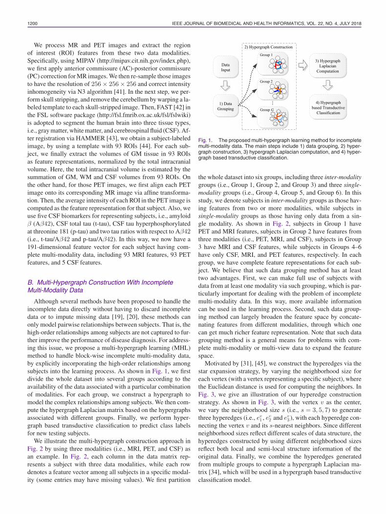
Although several methods have been proposed to handle theincomplete data directly without having to discard incompletedata or to impute missing data [19], [20], these methods canonly model pairwise relationships between subjects. That is, thehigh-order relationships among subjects are not captured to fur-ther improve the performance of disease diagnosis. For address-ing this issue, we propose a multi-hypergraph learning (MHL)method to handle block-wise incomplete multi-modality data,by explicitly incorporating the high-order relationships amongsubjects into the learning process. As shown in Fig. 1, we firstdivide the whole dataset into several groups according to theavailability of the data associated with a particular combinationof modalities. For each group, we construct a hypergraph tomodel the complex relationships among subjects. We then com-pute the hypergraph Laplacian matrix based on the hypergraphsassociated with different groups. Finally, we perform hyper-graph based transductive classification to predict class labelsfor new testing subjects.

We illustrate the multi-hypergraph construction approach inFig. 2 by using three modalities (i.e., MRI, PET, and CSF) asan example. In Fig. 2, each column in the data matrix rep-resents a subject with three data modalities, while each rowdenotes a feature vector among all subjects in a specific modal-ity (some entries may have missing values). We first partition

Fig. 1. The proposed multi-hypergraph learning method for incompletemulti-modality data. The main steps include 1) data grouping, 2) hyper-graph construction, 3) hypergraph Laplacian computation, and 4) hyper-graph based transductive classification.

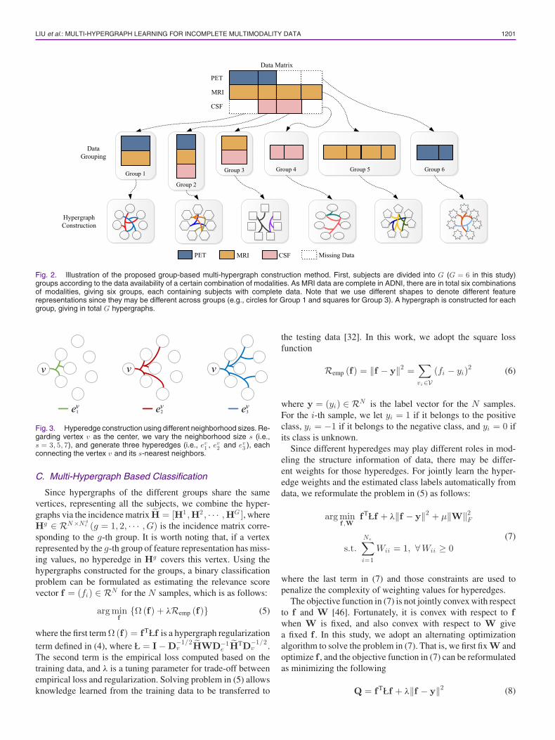
the whole dataset into six groups, including three inter-modalitygroups (i.e., Group 1, Group 2, and Group 3) and three single-modality groups (i.e., Group 4, Group 5, and Group 6). In thisstudy, we denote subjects in inter-modality groups as those hav-ing features from two or more modalities, while subjects insingle-modality groups as those having only data from a sin-gle modality. As shown in Fig. 2, subjects in Group 1 havePET and MRI features, subjects in Group 2 have features fromthree modalities (i.e., PET, MRI, and CSF), subjects in Group3 have MRI and CSF features, while subjects in Groups 4–6have only CSF, MRI, and PET features, respectively. In eachgroup, we have complete feature representations for each sub-ject. We believe that such data grouping method has at leasttwo advantages. First, we can make full use of subjects withdata from at least one modality via such grouping, which is par-ticularly important for dealing with the problem of incompletemulti-modality data. In this way, more available informationcan be used in the learning process. Second, such data group-ing method can largely broaden the feature space by concate-nating features from different modalities, through which onecan get much richer feature representation. Note that such datagrouping method is a general means for problems with com-plete multi-modality or multi-view data to expand the featurespace.

Motivated by [31], [45], we construct the hyperedges via thestar expansion strategy, by varying the neighborhood size foreach vertex (with a vertex representing a specific subject), wherethe Euclidean distance is used for computing the neighbors. InFig. 3, we give an illustration of our hyperedge constructionstrategy. As shown in Fig. 3, with the vertex v as the center,we vary the neighborhood size s (i.e., s = 3, 5, 7) to generatethree hyperedges (i.e., ev

1 , ev2 and ev

3 ), with each hyperedge con-necting the vertex v and its s-nearest neighbors. Since differentneighborhood sizes reflect different scales of data structure, thehyperedges constructed by using different neighborhood sizesreflect both local and semi-local structure information of theoriginal data. Finally, we combine the hyperedges generatedfrom multiple groups to compute a hypergraph Laplacian ma-trix [34], which will be used in a hypergraph based transductiveclassification model.


Fig. 2. Illustration of the proposed group-based multi-hypergraph construction method. First, subjects are divided into G (G = 6 in this study)groups according to the data availability of a certain combination of modalities. As MRI data are complete in ADNI, there are in total six combinationsof modalities, giving six groups, each containing subjects with complete data. Note that we use different shapes to denote different featurerepresentations since they may be different across groups (e.g., circles for Group 1 and squares for Group 3). A hypergraph is constructed for eachgroup, giving in total G hypergraphs.

Fig. 3. Hyperedge construction using different neighborhood sizes. Re-garding vertex v as the center, we vary the neighborhood size s (i.e.,s = 3, 5, 7), and generate three hyperedges (i.e., ev

1 , ev2 and ev

3 ), eachconnecting the vertex v and its s-nearest neighbors.

C. Multi-Hypergraph Based Classification

Since hypergraphs of the different groups share the samevertices, representing all the subjects, we combine the hyper-graphs via the incidence matrix H = [H1 ,H2 , · · · ,HG ], whereHg ∈ RN ×N g

e (g = 1, 2, · · · , G) is the incidence matrix corre-sponding to the g-th group. It is worth noting that, if a vertexrepresented by the g-th group of feature representation has miss-ing values, no hyperedge in Hg covers this vertex. Using thehypergraphs constructed for the groups, a binary classificationproblem can be formulated as estimating the relevance scorevector f = (fi) ∈ RN for the N samples, which is as follows:

arg minf

{Ω(f) + λRemp (f)} (5)

where the first term Ω(f) = fTŁf is a hypergraph regularizationterm defined in (4), where Ł = I − D−1/2

v HWD−1e HTD−1/2

v .The second term is the empirical loss computed based on thetraining data, and λ is a tuning parameter for trade-off betweenempirical loss and regularization. Solving problem in (5) allowsknowledge learned from the training data to be transferred to

the testing data [32]. In this work, we adopt the square lossfunction

Remp (f) = ‖f − y‖2 =∑vi ∈V

(fi − yi)2 (6)

where y = (yi) ∈ RN is the label vector for the N samples.For the i-th sample, we let yi = 1 if it belongs to the positiveclass, yi = −1 if it belongs to the negative class, and yi = 0 ifits class is unknown.

Since different hyperedges may play different roles in mod-eling the structure information of data, there may be differ-ent weights for those hyperedges. For jointly learn the hyper-edge weights and the estimated class labels automatically fromdata, we reformulate the problem in (5) as follows:

arg minf ,W

fTŁf + λ‖f − y‖2 + μ‖W‖2F

s.t.Ne∑i=1

Wii = 1, ∀Wii ≥ 0(7)

where the last term in (7) and those constraints are used topenalize the complexity of weighting values for hyperedges.

The objective function in (7) is not jointly convex with respectto f and W [46]. Fortunately, it is convex with respect to fwhen W is fixed, and also convex with respect to W givea fixed f . In this study, we adopt an alternating optimizationalgorithm to solve the problem in (7). That is, we first fix W andoptimize f , and the objective function in (7) can be reformulatedas minimizing the following

Q = fTŁf + λ‖f − y‖2 (8)


By differentiating Q with respect to f , we obtain

f = (Ł + λI)−1y (9)

In the second step, we optimize W with the learned f in thefirst step. Denote Λ = fTD−1/2

v H, and the objective functionin (7) can be rewritten as follows

arg minW

fTŁf + μ‖W‖2F

s.t.Ne∑i=1

Wii = 1, ∀Wii ≥ 0(10)

Then, the partial derivative of (10) with respect to W is asfollows

∂

∂W

{fTŁf + μ‖W‖2

F + η

(Ne∑i=1

Wii − 1

)}= 0 (11)

⇒ W =ΛTΛD−1

e − ηI2μ

η =ΛD−1

e ΛT − 2μ

Ne(12)

The above-mentioned two steps are performed iteratively un-til convergence. In the experiments, the iteration number is fixedas 20 empirically.

IV. EXPERIMENTS

A. Methods for Comparison

In the experiments, we first compare our MHL methodwith four baseline imputation-based approaches. These base-line methods utilize various data imputation techniques to im-pute missing features, which are summarized in the following:

1) Zero. In this method, those missing values are simplyfilled with zeros. If we first normalize the original data tohave unit standard deviation and zero mean, this method isequal to the mean value imputation method. More specif-ically, those missing values are filled with the means ofvalues that are available in the same row.

2) k-Nearest Neighbor (KNN) [47], [48]. In KNN method,we simply fill the missing value with weighted mean ofits k-nearest neighbor rows. Specifically, we first iden-tify the feature rows that are most similar to the onewith the missing value via KNN algorithm, and then fillthat missing values with the weighted mean of values inneighboring rows. Similar to the study in [49], the weightfor a specific neighboring row is inversely proportionalto the Euclidean distance between this neighboring rowand the row with missing values.

3) Expectation Maximization (EM) [27]. This method im-putes the missing values using the expectation maximiza-tion algorithm. To be specific, in the E step, we firstestimate the mean and the covariance matrix from thefeature matrix, and then fill those missing values with es-timates from the previous M step (or initialized as zeros).In the M step, based on the available values, estimatedmean and covariance, we fill those missing elements with

conditional expectation values. Then, the mean and thecovariance will be re-estimated based on the filled fea-ture matrix. In EM method, the above mentioned twosteps will be repeated until convergence.

4) Singular Value Decomposition (SVD) [28]. The missingvalues are iteratively filled-in based on matrix completionwith the low-rank approximation. Specifically, we first fillthose missing values with initial guesses (e.g., zeros), fol-lowed by a singular value decomposition (SVD) processto generate a low-rank approximation of a filled-in matrix.Based on the low-rank estimation matrix, we will updatethe missing elements with their corresponding values inthis matrix. Similarly, we will perform SVD again to ob-tain a new updated matrix, and repeat such process untilconvergence.

We further compare our method with state-of-the-art meth-ods for dealing with incomplete multi-modality data in the fieldof neuroimaging analysis. These methods include: 1) incom-plete Multi-Source Feature (iMSF) learning [19], 2) Ingalha-likar’s Algorithm [50], 3) incomplete Source-Feature Selection(iSFS) [20] method, and 4) a matrix shrunk and completion(MSC) method [49]. In the following, we briefly introduce thesemethods.

1) Incomplete Multi-Source Feature (iMSF) Learning [19].Using the similar data grouping technique as in ourmethod, iMSF regards the classification problem with in-complete multi-modality data as a sparse multi-task learn-ing problem, without discarding or imputing incompletedata. As shown in [19], iMSF is effective in finding in-formative features from incomplete multi-modality data.Two versions of iMSF are available based on two par-ticular loss functions (i.e., least squares loss and logisticloss), including least-squares (iMSF-Least) and logisticloss (iMSF-Logistic).

2) Ingalhalikar’s Algorithm [50]. In this method, an ensem-ble classification technique is used to fuse outputs of mul-tiple classifiers, where these classifiers are built based ondifferent subsets of subjects with complete feature repre-sentations. Specifically, this method first groups the origi-nal incomplete multi-modality data into multiple subsets,and then adopts the signal-to-noise ratio coefficient filteralgorithm to perform feature selection. Using those se-lected features, it constructs a linear discriminant analysis(LDA) [51] classifier in each individual subset. Finally,the classification results from all subjects are fused by aparticular ensemble strategy for making a final decisionfor a new testing subject. Two versions of this methodare available based on different ensemble strategies. Thefirst one, denoted as Ingalhalikar-Weighted, adopts theweighted averaging strategy, where each classifier is as-signed a particular weight based on its classification er-ror on the training data. The second one, denoted asIngalhalikar-Average, is based on the averaging strategy,where all classifiers are assigned equal weights.

3) Incomplete Source-Feature Selection (iSFS) method [20].In iSFS, subjects with incomplete multi-modality dataare first partitioned into several groups according to the


availability of data modalities. Then, a feature learningmodel is developed to find the most informative featuresfrom different data groups. That is, all subjects can beused in this method, without any discarding or imputationoperation.

4) Matrix Shrinkage and Completion (MSC) method [49].In MSC, the input features and the output label vec-tor are first combined into an incomplete matrix. Then,this incomplete matrix is further partitioned into sev-eral sub-matrices, with each one containing subjects withcomplete feature representation (w.r.t. certain combina-tions of multi-modalities). A multi-task learning model isadopted to select both discriminative features and infor-mative samples in each individual sub-matrix, leading to ashrunk matrix. Based on an EM imputation method [27],MSC finally completes those missing feature values andunknown target outputs of the shrunk matrix.

In this study, the proposed MHL method, Ingalhalikar’s algo-rithm, and MSC can directly perform classification tasks basedon incomplete multi-modality data. The other methods need toeither impute the missing data (e.g., Zero, KNN, EM, and SVD)or select a subset of features (e.g., iMSF, and iSFS). Motivatedby [19], [20], in the experiments, we adopt support vector ma-chine (SVM) for classification [52] after data imputation usingZero/KNN/EM/SVD and feature selection using iMSF/iSFS. Alinear SVM is used in the experiments, since the max-marginclassification nature of the linear SVM results in good general-izability [20].

B. Experimental Settings

We adopt a 10-fold cross-validation strategy [24] for per-formance evaluation. The subjects are partitioned into 10 sub-sets, and each subset has roughly equal number of subjects.Each time one subset is used as the testing set, while the re-maining 9 subsets are adopted as the training set. In orderto avoid any bias introduced by random partitioning of thedata, such process is repeated 10 times, and we record theaverage classification results. To optimize parameters for dif-ferent methods, we further perform an inner 10-fold cross-validation using each training set. Specifically, we furtherpartition each training set into 10 subsets for cross-validation pa-rameter selection [20]. Similar to [19], the neighborhood size kfor KNN is selected from {3, 5, 7, 9, 11, 15, 20}. For the SVD-based imputation method, the rank parameter is chosen from{5, 10, 15, 20, 25, 30}. The regularization parameter λ for iMSFis chosen from {10−5 , 10−4 , · · · , 101}. The parameters λ andμ for MHL and C for SVM are chosen from {10−3 , 10−2 ,· · · , 104}. The neighborhood sizes of {3, 5, 7, 9, 11, 15, 20} areused to construct multiple hyperedges in MHL. The influenceof the neighborhood size is discussed in Section V-D.

Seven metrics are used for performance evaluation: classi-fication accuracy (ACC), sensitivity (SEN), specificity (SPE),balanced accuracy (BAC), positive predictive value (PPV), neg-ative predictive value (NPV) and the area under the receiveroperating characteristic curve (AUC) [53]. Let TP, TN, FP, andFN denote True Positive, True Negative, False Positive, and

TABLE IIICOMPARISON WITH BASELINE IMPUTATION-BASED METHODS: AD VS. NC

CLASSIFICATION (%)

Zero KNN EM SVD MHL (Ours)

ACC 84.48 85.20 84.23 86.37 90.29SEN 77.96 70.98 67.76 80.78 84.40SPE 89.84 96.91 97.78 90.87 95.13BAC 83.90 83.94 82.77 85.82 89.77PPV 87.01 94.91 96.14 87.78 93.45NPV 83.36 80.31 78.82 85.64 88.11AUC 83.90 83.94 82.77 85.82 89.77

p-value 0.0017∗ 0.0014∗ 0.0038∗ 0.0037∗ −

TABLE IVCOMPARISON WITH BASELINE IMPUTATION-BASED METHODS: MCI VS. NC

CLASSIFICATION (%)

Zero KNN EM SVD MHL(ours)


p-value 0.0013∗ 0.0013∗ 0.0043∗ 0.0054∗ −

TABLE VCOMPARISON WITH BASELINE IMPUTATION-BASED METHODS: AD VS. MCI

CLASSIFICATION (%)



p-value 0.0051∗ 0.0056∗ 0.0024∗ 0.0013∗ −

False Negative, respectively. And the evaluation metrics are de-fined as: ACC = TP+TN

TP+TN+FP+FN ; SEN = TPTP+FN ; SPE = TN

TN+FP ;BAC = SEN+SPE

2 ; PPV = TPTP+FP ; NPV = TN

TN+FN . The McNemartest [54] is used to evaluate the statistical significance of thedifference between classification accuracies of two methods.We report the p-values in Tables III–VI and mark statisticallysignificant differences (p < 0.05) with the asterisk (∗).

C. Comparison With Baseline Methods

We first compare MHL with four baseline imputation-based methods, including Zero, KNN [47], [48], EM [27] andSVD [28]. In Tables III–VI, we report results for four clas-sification tasks: AD vs. NC, MCI vs. NC, AD vs. MCI, andpMCI vs. sMCI, respectively, where the best results are markedin boldface. We also show the receiver operating characteristic(ROC) curves achieved by different methods in Fig. 4. From


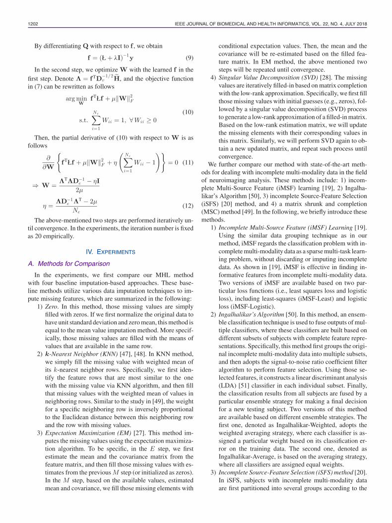
Fig. 4. ROC curves achieved by five different methods in (a) AD vs. NC, (b) MCI vs. NC, (c) AD vs. MCI, and (d) pMCI vs. sMCI classificationtasks. Here, different colors denote the ROC curves achieved by five different methods.

TABLE VICOMPARISON WITH BASELINE IMPUTATION-BASED METHODS: PMCI VS.

SMCI CLASSIFICATION (%)



p-value 0.0032∗ 0.0035∗ 0.0033∗ 0.0037∗ −

Tables III–VI and Fig. 4, we can observe that MHL consistentlyoutperforms the competing methods regarding all seven eval-uation criteria in four classification tasks. For instance, MHLachieves an accuracy of 90.29% and an AUC of 89.77% for ADvs. NC classification, outperforming other methods. The supe-riority of MHL is confirmed by the fact that the differences areall statistically significant as shown in the tables. On the otherhand, it is interesting to observe from Table V and Fig. 4(c) that,for AD vs. MCI classification, the sensitivity achieved by MHLand other methods are low. This implies that it is difficult todistinguish AD from MCI, because MCI (the prodrome of AD)might manifest abnormalities similar to AD.

D. Comparison With State-of-the-Art Methods

We further compare MHL with six state-of-the-art methodsfor AD/MCI classification, including two versions of Ingalha-likar’s algorithm (i.e., Ingalhalikar-Weighted, and Ingalhalikar-Average) [50], two versions of iMSF (i.e., iMSF-Least, andiMSF-Logistic) [19], iSFS [20], and MSC [49]. The results fordifferent classification tasks are reported in Tables VII–X. Notethat in these tables, we directly report the results of iSFS [20]and MSC [49] in their respective reference papers. FromTables VII–X, we can observe that the proposed MHL methodachieves the best ACC values in four classification tasks, andoutperforms six competing methods regarding AUC in both ADvs. MCI and pMCI vs. sMCI classification tasks.

E. Computational Complexity

According to Section III-B, the computational complexity forhypergraph construction is O(GN 2), where G is the number of

TABLE VIICOMPARISON WITH STATE-OF-THE-ART METHODS: AD VS. NC

CLASSIFICATION (%)

ACC SEN SPE AUC

Ingalhalikar-Weighted 83.03 78.54 86.72 89.82Ingalhalikar-Average 81.07 76.37 84.94 87.39iMSF-Least 86.41 76.91 94.24 85.57iMSF-Logistic 86.97 75.78 93.90 86.34iSFS 88.48 88.95 88.16 88.56MSC 88.50 83.70 92.70 94.40MHL(ours) 90.29 84.40 95.13 89.77

TABLE VIIICOMPARISON WITH STATE-OF-THE-ART METHODS: MCI VS. NC

CLASSIFICATION (%)

ACC SEN SPE AUC

Ingalhalikar-Weighted 62.58 65.42 57.73 64.40Ingalhalikar-Average 61.61 64.16 57.28 62.07iMSF-Least 70.64 81.62 54.42 63.02iMSF-Logistic 71.61 82.83 54.73 63.78MSC 71.50 75.30 64.90 77.30MHL(ours) 74.35 86.25 53.74 70.01

TABLE IXCOMPARISON WITH STATE-OF-THE-ART METHODS: AD VS. MCI

CLASSIFICATION (%)

ACC SEN SPE AUC

Ingalhalikar-Weighted 63.44 47.51 66.22 63.24Ingalhalikar-Average 63.10 45.46 65.71 61.69iMSF-Least 73.44 23.68 96.95 60.31iMSF-Logistic 73.96 25.36 96.95 61.16MHL(ours) 79.65 39.24 98.73 69.98

TABLE XCOMPARISON WITH STATE-OF-THE-ART METHODS: PMCI VS. SMCI

CLASSIFICATION (%)

ACC SEN SPE AUC

Ingalhalikar-Weighted 62.58 65.42 57.73 64.40Ingalhalikar-Average 61.61 64.16 57.28 62.07iMSF-Least 70.64 71.62 54.42 63.02iMSF-Logistic 71.61 72.83 54.73 63.78MHL(ours) 74.68 68.49 79.47 71.98


TABLE XIRUNTIME COMPARISON OF DIFFERENT METHODS IN AD VS. NC

CLASSIFICATION

Method Time (s)

Zero 0.48KNN 1.55EM 1.93SVD 2.92Ingalhalikar-Weighted 2.55Ingalhalikar-Average 2.35iMSF-Least 2.71iMSF-Logistic 4.16MHL(ours) 4.01

data grouping (e.g., G = 6 for ADNI with MRI, PET and CSFdata modalities), and N is the number of subjects in the database.Besides, the computational complexity for the hypergraph reg-ularized transductive classification is O(N 2T ), where T is theiteration number for solving the optimization problem in (7).Hence, the overall computational complexity of the proposedMHL method is O(N 2).

We further empirically compare the computational time costbetween MHL and 8 competing methods. Table XI reports thecomputational time costs of different methods in AD vs. NCclassification. From Tables VII and XI , we can see that thecomputational time cost of MHL is similar to that of iMSF-Logistic, while the classification results achieved by MHL aremuch higher than those of iMSF-Logistic.

V. DISCUSSION

We compare MHL with a simple graph method and a single-modality method in Sections V-A and V-B, respectively. InSection V-C, MHL is further compared with the commonlyused classifier, i.e., SVM. Sections V-D and V-E investigate theinfluences of neighborhood size in hyperedge construction andregularization parameters.

A. Comparison With Simple Graph

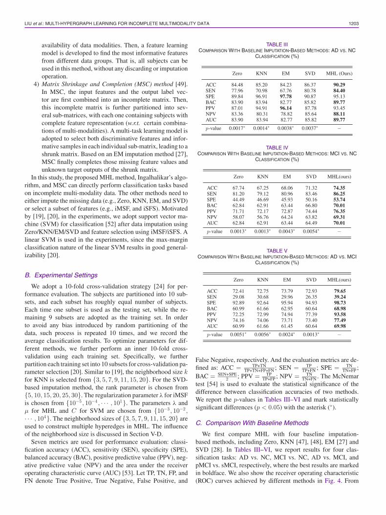
We compare MHL with a simple graph method (Simple-Graph), which is based on [34] and uses the normalized graphLaplacian for transductive classification. Note that a simplegraph can only model pairwise relationships among subjects.Similar to MHL, the regularization parameter in SimpleGraphis selected from {10−3 , 10−2 , · · · , 104} via cross validation.Fig. 5 shows that MHL achieves better results in most cases.For instance, MHL is superior to SimpleGraph in AD vs. MCIand pMCI vs. sMCI classification. These results support the factthat explicitly modeling complex relationships among subjectscan boost the learning performance.

B. Comparison With Single-Modality

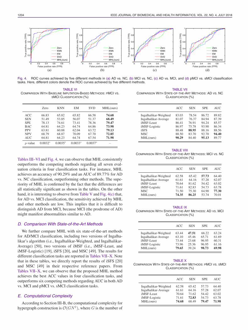
In the proposed MHL method, we use not only single-modality data, but also inter-modality data (with features frommore than one modalities). We now investigate whether usinginter-modality data can improve diagnosis performance. We run

Fig. 5. Comparison of MHL with a simple graph (SimpleGraph)method. (a) AD vs. NC classification. (b) MCI vs. NC classification.(c) AD vs. MCI classification. (d) pMCI vs. sMCI classification.

Fig. 6. Comparison of MHL with MHL-1, where MHL-1 only usessingle-modality data (i.e., MRI, PET, and CSF) to construct hypergraphs.(a) AD vs. NC classification. (b) MCI vs. NC classification. (c) AD vs. MCIclassification. (d) pMCI vs. sMCI classification.

MHL with data from only one single-modality (i.e., data inGroups 4–6 in Fig. 2) that is called MHL-1 in this paper. Fig. 6shows that MHL performs better than MHL-1 in all cases, indi-cating that inter-modality data improve the diagnostic accuracy.

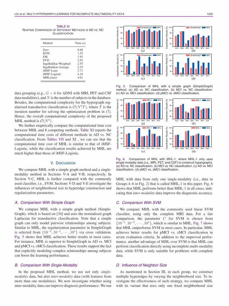
C. Comparison With SVM

We compare MHL with the commonly used linear SVMclassifier, using only the complete MRI data. For a faircomparison, the parameter C for SVM is chosen from{10−3 , 10−2 , · · · , 104}, which is similar to MHL. Fig. 7 showsthat MHL outperforms SVM in most cases. In particular, MHLachieves better results for pMCI vs. sMCI classification inseven evaluation criteria. In addition to the improved perfor-mance, another advantage of MHL over SVM is that MHL canperform classification directly using incomplete multi-modalitydata, while SVM is only suitable for problems with completedata.

D. Influence of Neighbor Size

As mentioned in Section III, in each group, we constructmultiple hyperedges by varying the neighborhood size. To in-vestigate the effectiveness of such strategy, we compare MHLwith its variant that uses only one fixed neighborhood size


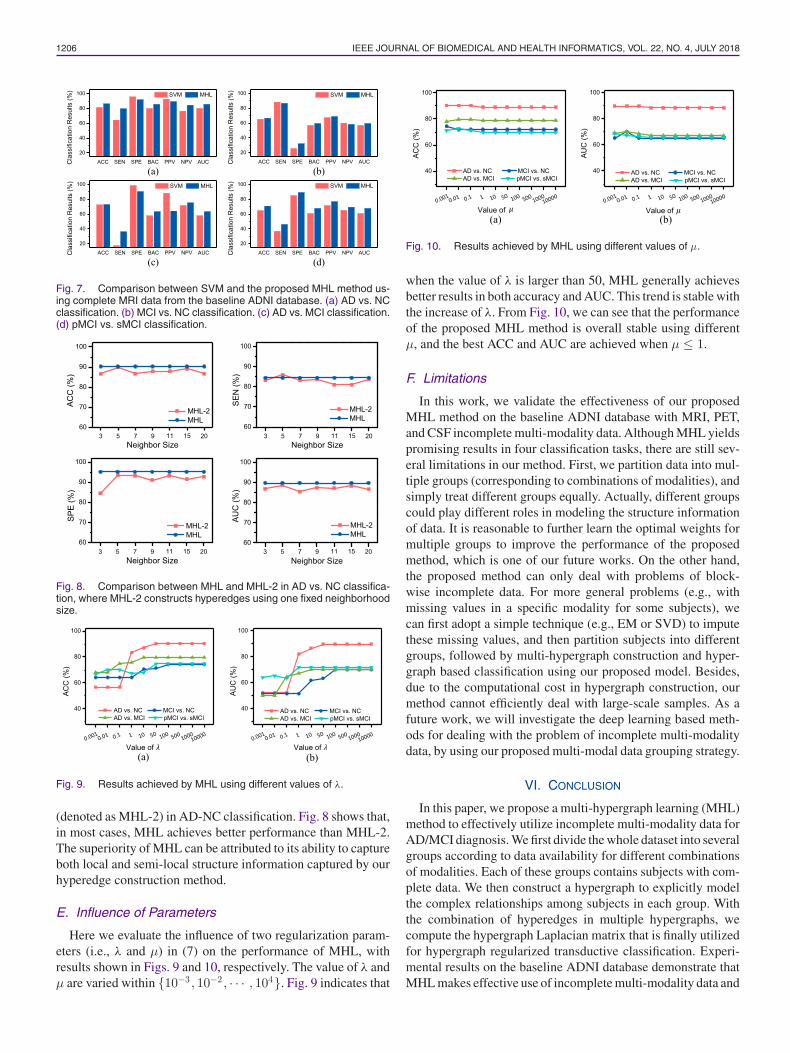
Fig. 7. Comparison between SVM and the proposed MHL method us-ing complete MRI data from the baseline ADNI database. (a) AD vs. NCclassification. (b) MCI vs. NC classification. (c) AD vs. MCI classification.(d) pMCI vs. sMCI classification.

Fig. 8. Comparison between MHL and MHL-2 in AD vs. NC classifica-tion, where MHL-2 constructs hyperedges using one fixed neighborhoodsize.

Fig. 9. Results achieved by MHL using different values of λ.

(denoted as MHL-2) in AD-NC classification. Fig. 8 shows that,in most cases, MHL achieves better performance than MHL-2.The superiority of MHL can be attributed to its ability to captureboth local and semi-local structure information captured by ourhyperedge construction method.

E. Influence of Parameters

Here we evaluate the influence of two regularization param-eters (i.e., λ and μ) in (7) on the performance of MHL, withresults shown in Figs. 9 and 10, respectively. The value of λ andμ are varied within {10−3 , 10−2 , · · · , 104}. Fig. 9 indicates that

Fig. 10. Results achieved by MHL using different values of μ.

when the value of λ is larger than 50, MHL generally achievesbetter results in both accuracy and AUC. This trend is stable withthe increase of λ. From Fig. 10, we can see that the performanceof the proposed MHL method is overall stable using differentμ, and the best ACC and AUC are achieved when μ ≤ 1.

F. Limitations

In this work, we validate the effectiveness of our proposedMHL method on the baseline ADNI database with MRI, PET,and CSF incomplete multi-modality data. Although MHL yieldspromising results in four classification tasks, there are still sev-eral limitations in our method. First, we partition data into mul-tiple groups (corresponding to combinations of modalities), andsimply treat different groups equally. Actually, different groupscould play different roles in modeling the structure informationof data. It is reasonable to further learn the optimal weights formultiple groups to improve the performance of the proposedmethod, which is one of our future works. On the other hand,the proposed method can only deal with problems of block-wise incomplete data. For more general problems (e.g., withmissing values in a specific modality for some subjects), wecan first adopt a simple technique (e.g., EM or SVD) to imputethese missing values, and then partition subjects into differentgroups, followed by multi-hypergraph construction and hyper-graph based classification using our proposed model. Besides,due to the computational cost in hypergraph construction, ourmethod cannot efficiently deal with large-scale samples. As afuture work, we will investigate the deep learning based meth-ods for dealing with the problem of incomplete multi-modalitydata, by using our proposed multi-modal data grouping strategy.

VI. CONCLUSION

In this paper, we propose a multi-hypergraph learning (MHL)method to effectively utilize incomplete multi-modality data forAD/MCI diagnosis. We first divide the whole dataset into severalgroups according to data availability for different combinationsof modalities. Each of these groups contains subjects with com-plete data. We then construct a hypergraph to explicitly modelthe complex relationships among subjects in each group. Withthe combination of hyperedges in multiple hypergraphs, wecompute the hypergraph Laplacian matrix that is finally utilizedfor hypergraph regularized transductive classification. Experi-mental results on the baseline ADNI database demonstrate thatMHL makes effective use of incomplete multi-modality data and


improves AD/MCI diagnostic accuracy. MHL is general and canbe extended to other problems with incomplete multi-modalitydata, such as those involved in longitudinal studies.

ACKNOWLEDGMENT

Data used in preparation of this article were obtained from theAlzheimer’s Disease Neuroimaging Initiative (ADNI) database.The investigators within the ADNI contributed to the designand implementation of ADNI and/or provided data but didnot participate in analysis or writing of this study. A com-plete listing of ADNI investigators can be found online https://adni.loni.usc.edu/wp-content/uploads/how_to_apply/ADNI_Acknowledgement_List.pdf.

REFERENCES

[1] R. Brookmeyer, E. Johnson, K. Ziegler-Graham, and H. M. Arrighi, “Fore-casting the global burden of Alzheimer’s disease,” Alzheimer’s Dementia,vol. 3, no. 3, pp. 186–191, 2007.

[2] A. Association et al., “2013 Alzheimer’s disease facts and figures,”Alzheimer’s Dementia, vol. 9, no. 2, pp. 208–245, 2013.

[3] E. M. Reiman, J. B. Langbaum, and P. N. Tariot, “Alzheimer’s preventioninitiative: A proposal to evaluate presymptomatic treatments as quickly aspossible,” Biomarkers Med., vol. 4, no. 1, pp. 3–14, 2010.

[4] R. Cuingnet et al., “Automatic classification of patients with Alzheimer’sdisease from structural MRI: A comparison of ten methods us-ing the ADNI database,” NeuroImage, vol. 56, no. 2, pp. 766–781,2011.

[5] R. Wolz et al., “Multi-method analysis of MRI images in early diagnosticsof Alzheimer’s disease,” PLoS ONE, vol. 6, no. 10, 2011, Art. no. e25446.

[6] J. Zhang, Y. Gao, Y. Gao, B. C. Munsell, and D. Shen, “Detecting anatom-ical landmarks for fast Alzheimer’s disease diagnosis,” IEEE Trans. Med.Imag., vol. 35, no. 12, pp. 2524–2533, Dec. 2016.

[7] F. Liu, L. Zhou, C. Shen, and J. Yin, “Multiple kernel learning in the pri-mal for multimodal Alzheimer’s disease classification,” IEEE J. Biomed.Health Informat., vol. 18, no. 3, pp. 984–990, May 2014.

[8] J. Zhang, M. Liu, L. An, Y. Gao, and D. Shen, “Alzheimer’sdisease diagnosis using landmark-based features from longitudinalstructural MR images,” IEEE J. Biomed. Health Informat., doi:10.1119/JBHI.2017.2704614, 2017.

[9] E. E. Bron, M. Smits, W. J. Niessen, and S. Klein, “Feature selectionbased on the SVM weight vector for classification of dementia,” IEEE J.Biomed. Health Informat., vol. 19, no. 5, pp. 1617–1626, Sep. 2015.

[10] J. Zhang, M. Liu, and D. Shen, “Detecting anatomical landmarks fromlimited medical imaging data using two-stage task-oriented deep neuralnetworks,” IEEE Trans. Image Process., vol. 26, no. 10, pp. 4753–4764,Oct. 2017.

[11] M. Liu, D. Zhang, and D. Shen, “Relationship induced multi-templatelearning for diagnosis of Alzheimer’s disease and mild cognitive impair-ment,” IEEE Trans. Med. Imag., vol. 35, no. 6, pp. 1463–1474, Jun. 2016.

[12] G. Chetelat, B. Desgranges, V. De La Sayette, F. Viader, F. Eustache,and J.-C. Baron, “Mild cognitive impairment can FDG-PET predict whois to rapidly convert to Alzheimer’s disease?” Neurology, vol. 60, no. 8,pp. 1374–1377, 2003.

[13] K. Herholz et al., “Discrimination between Alzheimer dementia andcontrols by automated analysis of multicenter FDG PET,” NeuroImage,vol. 17, no. 1, pp. 302–316, 2002.

[14] N. L. Foster et al., “FDG-PET improves accuracy in distinguishing fron-totemporal dementia and Alzheimer’s disease,” Brain, vol. 130, no. 10,pp. 2616–2635, 2007.

[15] F. Li, L. Tran, K.-H. Thung, S. Ji, D. Shen, and J. Li, “A robust deepmodel for improved classification of AD/MCI patients,” IEEE J. Biomed.Health Informat., vol. 19, no. 5, pp. 1610–1616, Sep. 2015.

[16] C. Lian, S. Ruan, T. Denœux, F. Jardin, and P. Vera, “Selecting radiomicfeatures from FDG-PET images for cancer treatment outcome prediction,”Med. Image Anal., vol. 32, pp. 257–268, 2016.

[17] O. Hansson, H. Zetterberg, P. Buchhave, E. Londos, K. Blennow,and L. Minthon, “Association between CSF biomarkers and incipientAlzheimer’s disease in patients with mild cognitive impairment: A follow-up study,” Lancet Neurol., vol. 5, no. 3, pp. 228–234, 2006.

[18] T. Kawarabayashi, L. H. Younkin, T. C. Saido, M. Shoji, K. H.Ashe, and S. G. Younkin, “Age-dependent changes in brain, CSF,and plasma amyloid β protein in the tg2576 transgenic mouse modelof Alzheimer’s disease,” J. Neurosci., vol. 21, no. 2, pp. 372–381,2001.

[19] L. Yuan, Y. Wang, P. M. Thompson, V. A. Narayan, and J. Ye, “Multi-source feature learning for joint analysis of incomplete multiple hetero-geneous neuroimaging data,” NeuroImage, vol. 61, no. 3, pp. 622–632,2012.

[20] S. Xiang, L. Yuan, W. Fan, Y. Wang, P. M. Thompson, and J. Ye, “Bi-level multi-source learning for heterogeneous block-wise missing data,”NeuroImage, vol. 102, pp. 192–206, 2014.

[21] M. Liu, D. Zhang, and D. Shen, “View-centralized multi-atlas classifica-tion for Alzheimer’s disease diagnosis,” Human Brain Mapping, vol. 36,no. 5, pp. 1847–1865, 2015.

[22] X. Cao, J. Yang, Y. Gao, Y. Guo, G. Wu, and D. Shen, “Dual-core steerednon-rigid registration for multi-modal images via bi-directional imagesynthesis,” Med. Image Anal., doi: 10.1016/j.media.2017.05.004, 2017.

[23] C. R. Jack et al., “The Alzheimer’s disease neuroimaging initia-tive (ADNI): MRI methods,” J. Magn. Reson. Imag., vol. 27, no. 4,pp. 685–691, 2008.

[24] T. Hastie, R. Tibshirani, J. Friedman, and J. Franklin, “The elements ofstatistical learning: Data mining, inference and prediction,” Math. Intell.,vol. 27, no. 2, pp. 83–85, 2005.

[25] K. Lakshminarayan, S. A. Harp, R. P. Goldman, and T. Samad, “Imputa-tion of missing data using machine learning techniques,” in Proc. ACMSIGKDD Conf. Knowl. Discovery Data Mining, 1996, pp. 140–145.

[26] R. J. Little and D. B. Rubin, Statistical Analysis With Missing Data.Hoboken, NJ, USA: Wiley, 2014.

[27] T. Schneider, “Analysis of incomplete climate data: Estimation of meanvalues and covariance matrices and imputation of missing values,” J.Climate, vol. 14, no. 5, pp. 853–871, 2001.

[28] G. H. Golub and C. Reinsch, “Singular value decomposition and leastsquares solutions,” Numerische Mathematik, vol. 14, no. 5, pp. 403–420,1970.

[29] E. J. Candes and B. Recht, “Exact matrix completion via convex optimiza-tion,” Found. Comput. Math., vol. 9, no. 6, pp. 717–772, 2009.

[30] M. Liu, J. Zhang, P.-T. Yap, and D. Shen, “View-aligned hypergraph learn-ing for Alzheimer’s disease diagnosis with incomplete multi-modalitydata,” Med. Image Anal., vol. 36, pp. 123–134, 2017.

[31] J. Y. Zien, M. D. Schlag, and P. K. Chan, “Multilevel spectral hypergraphpartitioning with arbitrary vertex sizes,” IEEE Trans. Comput.-Aided Des.Integr. Circuits Syst., vol. 18, no. 9, pp. 1389–1399, Sep. 1999.

[32] T. Joachims, “Transductive inference for text classification using sup-port vector machines,” in Proc. 16th Int. Conf. Mach. Learn., 1999,pp. 200–209.

[33] S. Agarwal, K. Branson, and S. Belongie, “Higher order learning withgraphs,” in Proc. 23rd Int. Conf. Mach. Learn., 2006, pp. 17–24.

[34] D. Zhou, J. Huang, and B. Scholkopf, “Learning with hypergraphs: Clus-tering, classification, and embedding,” in Proc. Adv. Neural Inf. Process.Syst., 2006, pp. 1601–1608.

[35] F. Wang and C. Zhang, “Label propagation through linear neighborhoods,”IEEE Trans. Knowl. Data Eng., vol. 20, no. 1, pp. 55–67, Jan. 2008.

[36] C. Berge and E. Minieka, Graphs and Hypergraphs, vol. 7. Amsterdam,The Netherlands: North Holland, 1973.

[37] Y. Gao, M. Wang, D. Tao, R. Ji, and Q. Dai, “3-D object retrieval and recog-nition with hypergraph analysis,” IEEE Trans. Image Process., vol. 21,no. 9, pp. 4290–4303, Sep. 2012.

[38] A. R. Benson, D. F. Gleich, and J. Leskovec, “Higher-order organizationof complex networks,” Science, vol. 353, no. 6295, pp. 163–166, 2016.

[39] J. Rodriguez, “On the Laplacian spectrum and walk-regular hyper-graphs,” Linear Multilinear Algebra, vol. 51, no. 3, pp. 285–297,2003.

[40] M. Bolla, “Spectra, Euclidean representations and clusterings of hyper-graphs,” Discrete Math., vol. 117, no. 1, pp. 19–39, 1993.

[41] J. G. Sled, A. P. Zijdenbos, and A. C. Evans, “A nonparametric methodfor automatic correction of intensity nonuniformity in MRI data,” IEEETrans. Med. Imag., vol. 17, no. 1, pp. 87–97, Feb. 1998.

[42] Y. Zhang, M. Brady, and S. Smith, “Segmentation of brain MR im-ages through a hidden Markov random field model and the expectation-maximization algorithm,” IEEE Trans. Med. Imag., vol. 20, no. 1,pp. 45–57, Jan. 2001.

[43] D. Shen and C. Davatzikos, “HAMMER: Hierarchical attribute matchingmechanism for elastic registration,” IEEE Trans. Med. Imag., vol. 21,no. 11, pp. 1421–1439, Nov. 2002.


[44] N. Kabani, “A 3D neuroanatomical atlas of the human brain,” NeuroImage,vol. 7, no. 4, p. 717, 1998.

[45] Y. Gao, M. Wang, Z.-J. Zha, J. Shen, X. Li, and X. Wu, “Visual-textualjoint relevance learning for tag-based social image search,” IEEE Trans.Image Process., vol. 22, no. 1, pp. 363–376, Jan. 2013.

[46] S. Boyd and L. Vandenberghe, Convex Optimization. Cambridge, U.K.:Cambridge Univ. Press, 2004.

[47] T. Hastie, R. Tibshirani, G. Sherlock, M. Eisen, P. Brown, and D. Bot-stein, “Imputing missing data for gene expression arrays,” Tech. Rep.,1999.

[48] O. Troyanskaya et al., “Missing value estimation methods for DNA mi-croarrays,” Bioinformatics, vol. 17, no. 6, pp. 520–525, 2001.

[49] K.-H. Thung, C.-Y. Wee, P.-T. Yap, and D. Shen, “Neurodegenerative dis-ease diagnosis using incomplete multi-modality data via matrix shrinkageand completion,” NeuroImage, vol. 91, pp. 386–400, 2014.

[50] M. Ingalhalikar, W. A. Parker, L. Bloy, T. P. Roberts, and R. Verma, “Usingmultiparametric data with missing features for learning patterns of pathol-ogy,” in Medical Image Computing and Computer-Assisted Intervention–MICCAI 2012. New York, NY, USA: Springer-Verlag, 2012, pp. 468–475.

[51] S. Mikat, G. fitscht, J. Weston, B. Scholkopft, and K.-R. Mullert, “Fisherdiscriminant analysis with kernels,” Neural Netw. Signal Process., vol. 9,pp. 41–48, 1999.

[52] C.-C. Chang and C.-J. Lin, “Libsvm: A library for support vectormachines,” ACM Trans. Intell. Syst. Technol., vol. 2, no. 3, 2011,Art. no. 27.

[53] R. H. Fletcher, S. W. Fletcher, and G. S. Fletcher, Clinical Epidemiology:The Essentials. Baltimore, MD, USA: Williams & Wilkins, 2012.

[54] T. G. Dietterich, “Approximate statistical tests for comparing super-vised classification learning algorithms,” Neural Comput., vol. 10, no. 7,pp. 1895–1923, 1998.

Documents

Multi-Hypergraph Learning for Incomplete Multimodality Data