Embed Size (px)
Citation preview
1
MULTI-FIDELITY DESIGN OF AN INTEGRAL THERMAL PROTECTION SYSTEM FOR FUTURE SPACE VEHICLE DURING RE-ENTRY
By
ANURAG SHARMA
A DISSERTATION PRESENTED TO THE GRADUATE SCHOOL OF THE UNIVERSITY OF FLORIDA IN PARTIAL FULFILLMENT
OF THE REQUIREMENTS FOR THE DEGREE OF DOCTOR OF PHILOSOPHY
UNIVERSITY OF FLORIDA
2010

2
2010 Anurag Sharma

3
To my parents Jagdish Prasad Sharma and Sujata Sharma, sister Shraddha Sharma and all my family members

4
ACKNOWLEDGMENTS
I would like to acknowledge my advisors Dr. Bhavani Sankar and Dr. Raphael T.
Haftka for all their tutelage, support, and encouragement. Their patience in dealing with
the thousands of questions I had for them throughout the course of this research and
their advice were invaluable. I also sincerely thank my dissertation committee members
Dr. Peter Ifju, Dr. Nam Ho Kim and Dr. Jack Mecholsky for evaluating my research work
and my candidature for the PhD degree. I would also like to thank specially Dr. Kim for
his course on Advanced Finite Element Methods which helped me in understanding the
basics on how to write the input files in ABAQUS®. Finally I would like to thank all my
fellow lab mates.
5
TABLE OF CONTENTS
page
ACKNOWLEDGMENTS .................................................................................................. 4
TABLE OF CONTENTS .................................................................................................. 5
LIST OF FIGURES .......................................................................................................... 9
LIST OF ABBREVIATIONS ........................................................................................... 14
LIST OF SYMBOLS ...................................................................................................... 15
ABSTRACT ................................................................................................................... 17
CHAPTER
1 INTRODUCTION .................................................................................................... 19
Motivation ............................................................................................................... 19
Thermal Protection System ..................................................................................... 21
Requirements for a Thermal Protection System ..................................................... 22
Approaches ............................................................................................................. 24
Background on Past Thermal Protection System ................................................... 26
Integral Thermal Protection System ........................................................................ 31
Dissertation Organization or Outline ....................................................................... 35
2 FINITE ELEMENT BASED MICROMECHANICS MODELS OF THE INTEGRATED THERMAL PROTECTION SYSTEM............................................... 46
Corrugated Core Sandwich Structure ..................................................................... 46
Geometric Variables and Material Properties ......................................................... 49
Unit Cell Analysis .................................................................................................... 49
Periodic Boundary Conditions ................................................................................. 51
Transverse Shear Stiffness A44 and A55 .................................................................. 56
Results .................................................................................................................... 58
Stiffness Matrix of an Integrated Thermal Protection System Sandwich Panel ............................................................................................................. 59
Prediction of Transverse Shear Stiffness ......................................................... 61
Validation of Transverse Shear Stiffness.......................................................... 63
Parametric Studies of the Transverse Shear Stiffness and the Maximum Deflection ...................................................................................................... 64
Concluding Remarks .............................................................................................. 66
6
3 STRESS AND BUCKLING ANALYSIS UNDER PRESSURE AND THERMAL LOADS ON AN INTEGRATED THERMAL PROTECTION SYSTEM PANEL ........ 86
Uniform Pressure Loading Analysis ........................................................................ 88
Stresses due to Pressure Load using Reverse Homogenization ...................... 89
Local Deflection and Stresses in the Top Face Sheet ...................................... 89
Thermal Loading Analysis ....................................................................................... 90
Sub Structuring ....................................................................................................... 93
Buckling of an Integrated Thermal Protection System ............................................ 94
Results .................................................................................................................... 95
Integrated Thermal Protection System Out-of-Plane Displacement, Uniform Pressure Load ............................................................................................... 96
Integrated Thermal Protection System Local Stress due to Pressure Load ..... 97
Integrated Thermal Protection System Local Stress due to Thermal Load ...... 98
Displacements from Plate Deformations .......................................................... 99
Concluding Remarks .............................................................................................. 99
4 MULTI-FIDELITY DESIGN AND OPTIMIZATION ................................................ 123
Multi-Fidelity Design.............................................................................................. 124
Thermal Analysis ............................................................................................ 130
Pressure Analysis ........................................................................................... 133
Integrated Thermal Protection System Optimization ............................................. 135
Concluding Remarks ............................................................................................ 136
5 CONCLUSIONS ................................................................................................... 158
Summary .............................................................................................................. 158
Concluding Remarks ............................................................................................ 159
Recommendations ................................................................................................ 160
APPENDIX: MATERIAL PROPERTIES USED FOR THE RESEARCH WORK ......... 163
LIST OF REFERENCES ............................................................................................. 167
BIOGRAPHICAL SKETCH .......................................................................................... 174
7
LIST OF TABLES Table page 2-1 The six sets of periodic boundary conditions. ..................................................... 67
2-2 Additional periodic boundary conditions on rotations θx and θy when shell elements are used. ............................................................................................. 67
3-1 Percentage difference for buckling eigen value analysis under thermal load. .. 101
4-1 Ranges of various parameters of the integral thermal protection system panel. ................................................................................................................ 138
4-2 Errors in maximum stress ratio and minimum buckling eigen value for thermal loading. ................................................................................................ 138
4-3 Response surfaces comparison for maximum stress ratio in top face sheet under thermal load. ........................................................................................... 139
4-4 Response surfaces comparison for the maximum stress ratio in the web under thermal load. ........................................................................................... 140
4-5 Response surfaces comparison for maximum stress ratio in bottom face sheet under thermal load. ................................................................................. 141
4-6 Response surfaces comparison for minimum buckling eigen value under thermal load. ..................................................................................................... 142
4-7 Response surfaces comparison for maximum stress ratio in bottom face sheet under thermal load. ................................................................................. 143
4-8 Response surfaces comparison for the minimum buckling eigen value under thermal load. ..................................................................................................... 144
4-9 Errors in maximum stress, deflection and minimum buckling eigen value for pressure loading. .............................................................................................. 145
4-10 Response surfaces comparison for maximum stress in top face sheet under pressure load. ................................................................................................... 146
4-11 Response surfaces comparison for maximum stress in web under pressure load. .................................................................................................................. 146
4-12 Response surfaces comparison for maximum stress in bottom face sheet under pressure load. ......................................................................................... 147
4-13 Rsponse surfaces comparison for maximum top face sheet deflection under pressure load. ................................................................................................... 147
8
4-14 Response surfaces comparison for minimum buckling eigen value under pressure load. ................................................................................................... 148
4-15 Optimized design. ............................................................................................. 148
4-16 Constraints value at the optimum. .................................................................... 149
A-1 Thermal conductivity, specific heat, and coefficient of thermal expansion of titanium alloy. .................................................................................................... 163
A-2 Young‟s modulus and yield stress of titanium alloy. ......................................... 164
A-3 Thermal conductivity, specific heat, and coefficient of thermal expansion of beryllium alloy. .................................................................................................. 165
A-4 Young‟s modulus and yield stress of beryllium alloy. ........................................ 166
9
LIST OF FIGURES
Figure page 1-1 Space Shuttle photograph showing release point of 1.7-lb foam at the bipod
ramp and the impact point. ................................................................................. 37
1-2 Schematic and photograph (Space Shuttle Orbiter elevons) of an insulated structure. ............................................................................................................ 37
1-3 Schematic and photograph (X-15) of a heat sink structure. ................................ 38
1-4 Schematic and photograph of a hot structure. .................................................... 38
1-5 Schematic and photograph of a heat-pipe-cooled leading edge. ........................ 39
1-6 Schematic and photograph of an ablative heat shield. ....................................... 39
1-7 Schematic and photograph of actively convective cooling structure. .................. 40
1-8 Actively convective cooling panel. ...................................................................... 40
1-9 Schematic of film cooling and drawing of a hypersonic vehicle. ......................... 40
1-10 Schematic of transpiration cooling and a carbon/carbon cooled combustion chamber test article. ........................................................................................... 41
1-11 Schematic of reusable surface insulation installation. ........................................ 41
1-12 X-33 windward surface configuration. ................................................................. 42
1-13 Metallic thermal protection system concept for windward surface of X-33. ........ 42
1-14 Schematic drawing of the ceramic matrix composite thermal protection system. ............................................................................................................... 43
1-15 Advanced-adapted, robust, metallic, operable, reusable thermal protection system panel. ..................................................................................................... 43
1-16 Thermal protection system integrated with cryogenic tank. ................................ 44
1-17 Tailorable advanced blanket insulation thermal protection system. .................... 44
1-18 Conformal reusable insulation-blanket with rigidized outer surface. ................... 45
1-19 A corrugated-core sandwich structure concept for integrated thermal protection system. .............................................................................................. 45
1-20 Schematic diagram of two sandwich panels. ...................................................... 45
10
2-1 Corrugated cardboards. ...................................................................................... 67
2-2 Unit-cell of the corrugated-core sandwich structure. ........................................... 68
2-3 Integral thermal protection system panel is modeled as a homogeneous orthotropic plate. ................................................................................................. 68
2-4 nx is the outward unit normal, which has a value of +1 and -1 as shown and zero in the other faces. ....................................................................................... 69
2-5 Finite element model of the unit cell. .................................................................. 69
2-6 Typical mesh and finite element model for the estimation of transverse shear stiffness A55. ....................................................................................................... 70
2-7 Typical mesh and finite element model for the estimation of transverse shear stiffness A44. ....................................................................................................... 70
2-8 Three dimensional finite element model of the integral thermal protection system panel. ..................................................................................................... 71
2-9 Typical mesh and boundary conditions for the low fidelity two dimensional finite element model. .......................................................................................... 71
2-10 Unit cell deformations when periodic boundary conditions are imposed. ........... 72
2-11 Plate model subjected to uniform moment in order to validate the stiffness matrix in the x- direction. .................................................................................... 72
2-12 Three dimensional finite element model subjected to moment for stiffness verification along x- axis. .................................................................................... 73
2-13 Three dimensional and plate deflection comparison under moment for stiffness verification along x- axis. ...................................................................... 74
2-14 Three dimensional finite element model subjected to moment for stiffness verification along y- axis. .................................................................................... 75
2-15 Three dimensional and plate deflection comparison under moment for stiffness verification along y- axis. ...................................................................... 76
2-16 Transverse shear stiffness A44 as a function of the length of the beam when subjected to pressure load. ................................................................................ 77
2-17 Transverse shear stiffness A55 as a function of the length of the beam when subjected to pressure load. ................................................................................ 78
2-18 Undeformed and deformed shape of the three dimensional panel, when subjected to transverse pressure. ....................................................................... 79
11
2-19 Undeformed and deformed shape of the plate model, when subjected to transverse pressure. ........................................................................................... 80
2-20 Variation for the transverse shear stiffness A44 with web angle. ......................... 81
2-21 Variation for the transverse shear stiffness A55 with web angle. ......................... 82
2-22 Variation of maximum deflection of top face sheet with web angle under transverse load. .................................................................................................. 83
2-23 Percentage difference of maximum top face sheet deflection with the change in A44 under transverse load. .............................................................................. 84
2-24 Percentage difference of maximum top face sheet deflection with change in A55 under transverse load. .................................................................................. 85
3-1 Representation of the integral thermal protection system panel as a plate. ..... 101
3-2 Flowchart describing the homogenization and reverse homogenization method. ............................................................................................................ 101
3-3 Aerodynamic pressure load on the top face sheet for a space shuttle-like design.. ............................................................................................................. 102
3-4 Three dimensional finite element model when subjected to pressure load. ...... 103
3-5 Low fidelity plate model when subjected to pressure load. ............................... 103
3-6 Reverse homogenization for a two dimensional plate. ..................................... 104
3-7 Contour of von mises stresses in the integral thermal protection system due to pressure loading. .......................................................................................... 104
3-8 Local stresses and deflections of the top face sheet due to uniform pressure loading. ............................................................................................................. 105
3.9 Approximate heating rate used for the analysis. ............................................... 105
3-10 Variation of the temperature with respect to different reentry times. ................. 106
3-11 Constraining the unit cell to prevent displacements and strains in x and y directions. ......................................................................................................... 106
3-12 Thermal forces and moments resultants on to the two dimensional plate model. ............................................................................................................... 107
3-13 Reverse thermal forces and moments being applied to the two dimensional plate model. ...................................................................................................... 107
12
3-14 Typical web buckling modes of the integral thermal protection system panel under thermal loads. ......................................................................................... 108
3-15 Thermal buckling analysis of the unit cell. ........................................................ 109
3-16 Web buckling modes of the integral thermal protection system panel under pressure loads. ................................................................................................. 110
3-17 High fidelity three dimensional finite element model of one fourth of the panel. ................................................................................................................ 111
3-18 Typical mesh and boundary conditions for the low fidelity two dimensional finite element model. ........................................................................................ 111
3-19 Comparison of the plate and three dimensional bottom face sheet vertical deflections. ....................................................................................................... 112
3-20 Comparison of the plate and three dimensional top face sheet vertical deflections. ....................................................................................................... 113
3-21 Comparison of the plate and three dimensional top face sheet stresses under pressure load. ................................................................................................... 114
3-22 Comparison of the plate and three dimensional bottom face sheet stresses under pressure load. ......................................................................................... 115
3-23 Comparison of the plate and three dimensional top face sheet stresses under thermal load. ..................................................................................................... 116
3-24 Comparison of the plate and three dimensional bottom face sheet stresses under thermal load. ........................................................................................... 117
3-25 Computing u, v and w displacements along the y- direction from the plate displacements. .................................................................................................. 118
3-26 Comparison of the v and w displacements of the various components under pressure load at x = a/2. ................................................................................... 119
3-27 Comparison of the u, v and w displacements of the various components under pressure load at x = a/2-2p. .................................................................... 120
3-28 Comparison of the v and w displacements of the various components under thermal load at x = a/2. ..................................................................................... 121
3-29 Comparison of the u, v and w displacements of the various components under thermal load at x = a/2-2p. ...................................................................... 122
4-1 Corrugated-core sandwich structure with all the six design variables used for generating the response surface. ..................................................................... 150
13
4-2 Loss function used in the support vector regression. ........................................ 150
4-3 Three dimensional value is fitted as a linear function of a two dimensional plate values. ..................................................................................................... 151
4-4 Sensitivity indices for the maximum bottom face sheet stress ratio under thermal loading. ................................................................................................ 151
4-5 Sensitivity indices for the minimum buckling eigen value under thermal loading. ............................................................................................................. 152
4-6 Sensitivity indices for the maximum von mises top face sheet stress under pressure loading. .............................................................................................. 153
4-7 Sensitivity indices for the maximum von mises web stress under pressure loading. ............................................................................................................. 154
4-8 Sensitivity indices for the maximum von mises bottom face sheet stress under pressure loading. .................................................................................... 155
4-9 Sensitivity indices for the maximum top face sheet deflection under pressure loading. ............................................................................................................. 156
4-10 Sensitivity indices for the minimum buckling eigen value under pressure loading. ............................................................................................................. 157
5-1 Sandwich structure with web corrugations in both x- and y- directions. ............ 162
14
LIST OF ABBREVIATIONS
AFRSI advanced flexible reusable surface insulation
ARMOR advanced-adapted, robust, metallic, operable, reusable
CEV crew exploration vehicle
CRS correction response surface
FEA finite element analysis
FEM finite element method
FRCI fibrous refractory composite insulation
HRSI high-temperature reusable surface insulation
ITPS integrated thermal protection system
LRSI low-temperature reusable surface insulation
NASA National Aeronautics and Space Administration
PRS polynomial response surface
RCC reinforced carbon-carbon
RLV reusable launch vehicle
RSA response surface approximations
RSI reusable surface insulation
SSTO single-stage-to-orbit
TPS thermal protection system
2D two-dimensional
3D three-dimensional

15
LIST OF SYMBOLS
a panel length (x-direction)
A44 shearing stiffness (y-direction)
A55 shearing stiffness (x-direction)
[A] extensional stiffness matrix
[B] coupling stiffness matrix
b panel width (y-direction)
[D] bending stiffness matrix
'
11D reduced stiffness matrix (x-direction)
'
22D reduced stiffness matrix (y-direction)
d height of the sandwich panel
0 midplane strain
curvature
Lex length of the cantilever beam (x-direction)
Ley length of the cantilever beam (y-direction)
M moment resultant
MT thermal moment resultant
N force resultant
NT thermal force resultant
2p unit cell length
Po pressure acting on the cantilever beam
Qx, Qy transverse shear force
s web length
tT, tTF top face sheet thickness
tBF bottom face sheet thickness
16
tW web thickness
θ web inclination
u unit cell displacement (x-direction)
u0 (x,y) mid-plane displacement (x-direction)
v unit cell displacement (y-direction)
v0 (x,y) mid-plane displacement (y-direction)
w unit cell vertical displacement (z-direction)
( , ), ( , )x yx y x y rotations of plate‟s cross section
,x y global rotations
,xz yz transverse shear strains
Multi FidelityS multi-fidelity response surface approximations
3DS high-fidelity response surface approximations
2DS low-fidelity response surface approximations
_Diff CRSS CRS based on the difference between 3D and 2D
_Ratio CRSS CRS based on the ratio between 3D and 2D
17
Abstract of Dissertation Presented to the Graduate School of the University of Florida in Partial Fulfillment of the Requirements for the Degree of Doctor of Philosophy
MULTI-FIDELITY DESIGN OF AN INTEGRAL THERMAL PROTECTION SYSTEM
FOR FUTURE SPACE VEHICLE DURING RE-ENTRY
By
Anurag Sharma
December 2010
Chair: Bhavani V. Sankar Co-Chair: Raphael T. Haftka Major: Mechanical Engineering
The primary function of a thermal protection system (TPS) is to protect the space
vehicle from extreme aerodynamic heating and to maintain the underlying structure
within acceptable temperature limits. Currently used TPS are not load bearing
members. One potential method of saving weight is to have a load-bearing TPS that
performs both thermal and structural functions. One such concept called the Integrated
Thermal Protection System (ITPS) uses a corrugated-core sandwich structure.
Optimization of an ITPS requires thousands of three-dimensional (high-fidelity model)
simulations, which is very expensive. Hence, a finite element (FE) based
homogenization procedure is developed in which the ITPS is modeled as an equivalent
orthotropic plate. The results for deflection and stresses obtained using the plate model
(low fidelity model) are not very accurate. The high-fidelity model is analyzed at only few
designs in order to reduce the cost, and these results in errors in the response surfaces
based only on the high-fidelity model. To resolve this difficulty, the low fidelity two-
dimensional (2D) plate models is fitted with a high quality surrogate, which is then
corrected by using a small number of high fidelity three-dimensional (3D) finite element
18
analyses. Fitting the difference or the ratio between the high fidelity analyses and the
low fidelity surrogate with a response surface approximation allows construction of the
so called correction response surface. This multi-fidelity or variable-complexity modeling
requires significantly fewer high fidelity analyses for a given accuracy.
A MATLAB® and a JAVA code has been developed in conjunction with the
Surrogate Toolbox in order to carry out these FE analyses automatically using
ABAQUS®. The multi-fidelity response surface approximation (RSA) is used to optimize
the mass of the ITPS for a given material combination and loading conditions. For the
same given accuracy, multi-fidelity response surface took 30 percent less time as
compared to the full 3D response surface. Further, one can choose the best correction
model based on the data without the test points, and the test points also confirmed the
choice.

19
CHAPTER 1 INTRODUCTION
Motivation
Space exploration has always been a source of national pride for United States as
well for others. It is a valuable tool in our quest to understand the universe. The Hubble
Space Telescope provides us with an understanding of the history of our galaxy and
offers a glimpse into others. Satellite programs like Solar Radiation and Climate
Experiment (SORCE) and Gravity Recovery and Climate Experiment (GRACE) gives us
the ability to fully take on the climate change crisis as a nation and a world. The
capabilities of spacecraft and other high-speed flight vehicles are being taken to exciting
new levels with ventures like the International Space Station and commercial space
programs like the ongoing space tourism and space-based communications. As we try
to fly farther, faster and more often, reusability of these flight vehicles becomes of
greater importance due to their reduced costs and decreased turnaround time between
flights. It is therefore important that decreasing the cost of launching a space vehicle is
one of the vital requirements of the space industry. The use of space is becoming more
regular, therefore future space vehicle needs to be completely reusable, have higher
functional extensibility, and have a lower running cost than the existing Space Shuttle
[5].
One of the NASA‟s foremost goals has been to lessen the cost of carrying a pound
of payload by an order of magnitude [6]. It has been found that a single-stage-to-orbit
(SSTO) reusable launch vehicle (RLV) can help to achieve this target. Regardless of
many challenges and difficulties, SSTO is something worth trying with such an
increased demand for space access. An expendable rocket vehicle, such as the

20
Russian Proton and US Delta offers one of the least costly ways to deliver a payload
with the payload cost varying from $4,000 to $20,000 per pound [7], but for every launch
a completely new launch vehicle is required. A major step towards reusability starts
with the improvement of the thermal protection system (TPS) of these vehicles. As we
push our boundaries beyond earth‟s lower orbit to Mars and beyond, new space
vehicles such as hypersonic Crew Exploration Vehicle (CEV), air breathing vehicles [1],
military space planes [2] and unmanned experiment return capsules [3] are being
developed, and TPS will be occupying a huge area on the exteriors and will form the
primary part of the launch weight. Since the TPS is such an expensive and intrinsic part
of the design of space vehicles [4], there will be new and interesting ideas to explore for
years to come.
The Space Shuttle which is not fully reusable, offers a good but a costly launch
system. One of the most expensive maintenance systems for the Shuttle Orbiter is the
TPS. Between flights the approximate maintenance time is 40,000 hours [8, 9].
Lockheed Martin came up with an SSTO design, i.e. Venture Star, which could reduce
the cost of launching a satellite by 1/10th as compared to the Space Shuttle [10].
However, due to many technological challenges the program was cancelled. Currently,
NASA is planning to use Ares I to launch Orion, the spacecraft being designed for
NASA human space flight missions after the Space Shuttle is retired in 2010.
It has been widely confirmed by the aerospace community that altogether
independent, reusable single-stage vehicle could decrease the costs considerably. In
future the reusable SSTOs would be the main focus of research as the cost of each
launch will be lessened by making a reusable sophisticated vehicle that launches at
21
regular quick intervals with minimal maintenance. Such vehicles will have an ample
region to be covered with TPS, because the fuel tanks will be an integral part required
for launch. As a result of the massive TPS coverage region, a need for a lightweight
TPS is essential to keep the vehicle launch cost and weight moderate and affordable.
The major reduction in the payload delivering costs is the rationale for the advancement
of a future space vehicle.
Thermal Protection System
Thermal Protection System (TPS) is the barrier that shields the space vehicle from
aerodynamic heating during atmospheric reentry. The atmospheric gas causes surface
friction and compression on the vehicle surface which results in high aerodynamic
heating. The vehicle's structure and entry path in combination with the kind of thermal
protection system used characterize the vehicle‟s temperature distribution [18]. High
reentry speeds greater than Mach 20 causes such heating, which is adequate enough
to damage the vehicle structure. The previous space vehicles such as Mercury, Gemini,
and Apollo had blunt bodies to give a “stand-off bow shock” [11 – 17]. The result is that
most of the heat is expended to the surrounding air. Furthermore, these vehicles had
ablative materials that change directly into gas at high temperature. The sublimation
action consumes thermal energy from high aerodynamic heating and wears away the
material from the surface. Thermal blankets and insulating tiles are used on the bottom
region of the Space Shuttle [9, 19] to consume and radiate heat while blocking
conduction to the aluminum substructure. It consists of approximately 25,000 tiles which
act as a heat resistant blanket. The black tiles on the bottom of the orbiter should be
able to bear 2,000 oF during reentry. During reentry, shock waves are generated on the
orbiter and those tiles are needed to protect the aluminum skin of the orbiter, which
22
cannot withstand temperatures over 350 oF without structural failure. Since the
temperatures can go up to 2,000 oF, this four inch thick tile has to dissipate a large
amount of heat. Further, these tiles are attached to the orbiter aluminum structure with a
strain isolation pad in between. If these tiles are attached directly to the aluminum, any
strains such as mechanical or thermal in the aluminum may cause substantial tensile
strains in the tiles, which could cause cracking.
Requirements for a Thermal Protection System
The principal objective of a TPS is to keep the temperature of the underlying
structure within specified limits. The TPS should be shielded from different types of
environments like the ground lightning strike, hail strike, bird strike, and on-orbit
debris/micro-meteoroid hypervelocity impact, etc [10]. The basic requirements that the
TPS should satisfy are given below and are similar to that mentioned in [20, 21].
Thermal Loading: TPS is subjected to varying temperature distributions. At a
given time, the side facing the sun will have a temperature of about 250 oF and the side
away from the sun will be at about -150 oF. TPS panels which are attached to cryogenic
fuel tanks are subjected to low temperatures before takeoff and also in space. Such
varying temperatures cause temperature gradient which can result in very high thermal
stresses and can also cause creep and other inelastic behavior at elevated
temperatures. In order to prevent the vehicle from catastrophic failure, the TPS should
be able to bear such varying temperatures at all flight environments [22].
Aerodynamic Pressure Load: The flight environments and space vehicle location
determine if the aerodynamic pressure load pulls the TPS panel off the vehicle or be
compressive in nature. The compressive pressure load could cause the outer surface,
loading attachments, and support hardware to bend considerably and thereby changing
23
the aerodynamic shape of the vehicle. The TPS should be able to avoid failure and
fracture under these varying pressure loads [10].
Panel Deformations: The panel deflection should be within acceptable bounds
under any given loading condition. The deformation could occur due to pressure,
thermal bowing or acoustic and dynamic loads. Depending on the space vehicle
location and flight environments, the deformation can vary considerably. However, for
any condition, premature transformation to turbulence (which would greatly escalate the
surface heating) [9], should be averted in order to maintain a suitable aerodynamic
surface.
Foreign Object Impact: TPS must be able to bear any foreign particle collision
under any flight environments. The impingement could be during launch and landing
from low speed debris, impacts at hypervelocity from on-orbit debris or/and from
weather related impacts such as hail and rain. The Space Shuttle Columbia was one of
the victims of such debris impact on the TPS tiles. The debris struck the leading edge of
the left wing, damaging the Shuttle's thermal protection system (TPS) [28] (Figure 1-1).
Chemical Corrosion: At very extreme temperatures, TPS materials become
sensitive to oxidation. TPS properties may change significantly due to this chemical
attack. This results in further degradation in structural performance and temperature
capabilities. TPS material should be resistant towards chemical corrosion.
For RLV‟s, decreasing the mass of the TPS has been the primary focus for
making the efficiency better. Vehicle with reduced mass requires fewer energy and
fuel, thereby carrying more payloads. Vehicle‟s performance can be increased further
24
by using a better material and coating to enhance TPS performance so that it could
perform in more extreme thermal environments.
Decreasing the cost of the TPS has become a main issue, with more use of RLV‟s
for various civilian and military applications. Enhanced design and newer analysis
procedures, approaches, materials, coatings and fabrication and installation methods
need to be evolved in order to lessen the costs [9]. Cost reduction could be increased
further by making it more durable and robust. Further improving these attributes will also
decrease the cost and time for repair and replacements, as they will have greater
resistance to impact and handling damages. All of these will decrease the recurring
costs; enhance the working envelope of the vehicle and thereby allowing movement in
all environments and rapid turnaround between flights [23]. All these attributes are
strongly interdependent, often directly conflicting, and require compromises in the
design process to reach an acceptable solution. Finally, the approach should lead to the
optimal combination of these features, such that a robust, operable and weight-efficient
TPS can be developed.
Approaches
Extreme thermal environments can be dealt in various ways during hypersonic
flight. As more air-breathing hypersonic vehicles are being developed, newer and
efficient ways to restricting these extreme temperatures need to be developed to meet
the severe thermal structural changes. These techniques include both TPS and hot
structures and these concepts can be commonly categorized as: passive, semi-passive,
and actively cooled approaches [24].
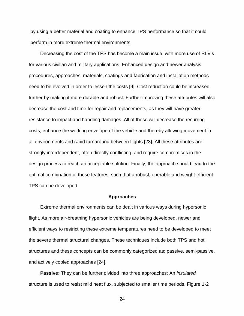
Passive: They can be further divided into three approaches: An insulated
structure is used to resist mild heat flux, subjected to smaller time periods. Figure 1-2
25
[24] shows the insulated structure for the Space Shuttle Orbiter elevons. Thermal
radiation is generally the mechanism to remove heat. It absorbs most of the heat
through insulation, thereby maintaining the structure beneath with an acceptable
temperature range.
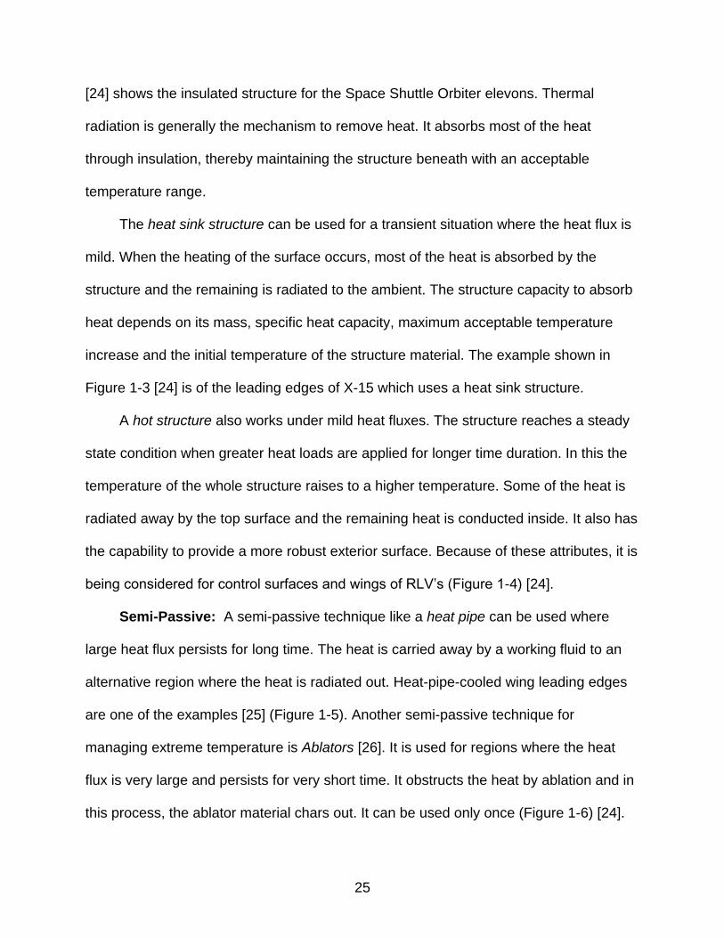
The heat sink structure can be used for a transient situation where the heat flux is
mild. When the heating of the surface occurs, most of the heat is absorbed by the
structure and the remaining is radiated to the ambient. The structure capacity to absorb
heat depends on its mass, specific heat capacity, maximum acceptable temperature
increase and the initial temperature of the structure material. The example shown in
Figure 1-3 [24] is of the leading edges of X-15 which uses a heat sink structure.
A hot structure also works under mild heat fluxes. The structure reaches a steady
state condition when greater heat loads are applied for longer time duration. In this the
temperature of the whole structure raises to a higher temperature. Some of the heat is
radiated away by the top surface and the remaining heat is conducted inside. It also has
the capability to provide a more robust exterior surface. Because of these attributes, it is
being considered for control surfaces and wings of RLV‟s (Figure 1-4) [24].
Semi-Passive: A semi-passive technique like a heat pipe can be used where
large heat flux persists for long time. The heat is carried away by a working fluid to an
alternative region where the heat is radiated out. Heat-pipe-cooled wing leading edges
are one of the examples [25] (Figure 1-5). Another semi-passive technique for
managing extreme temperature is Ablators [26]. It is used for regions where the heat
flux is very large and persists for very short time. It obstructs the heat by ablation and in
this process, the ablator material chars out. It can be used only once (Figure 1-6) [24].
26
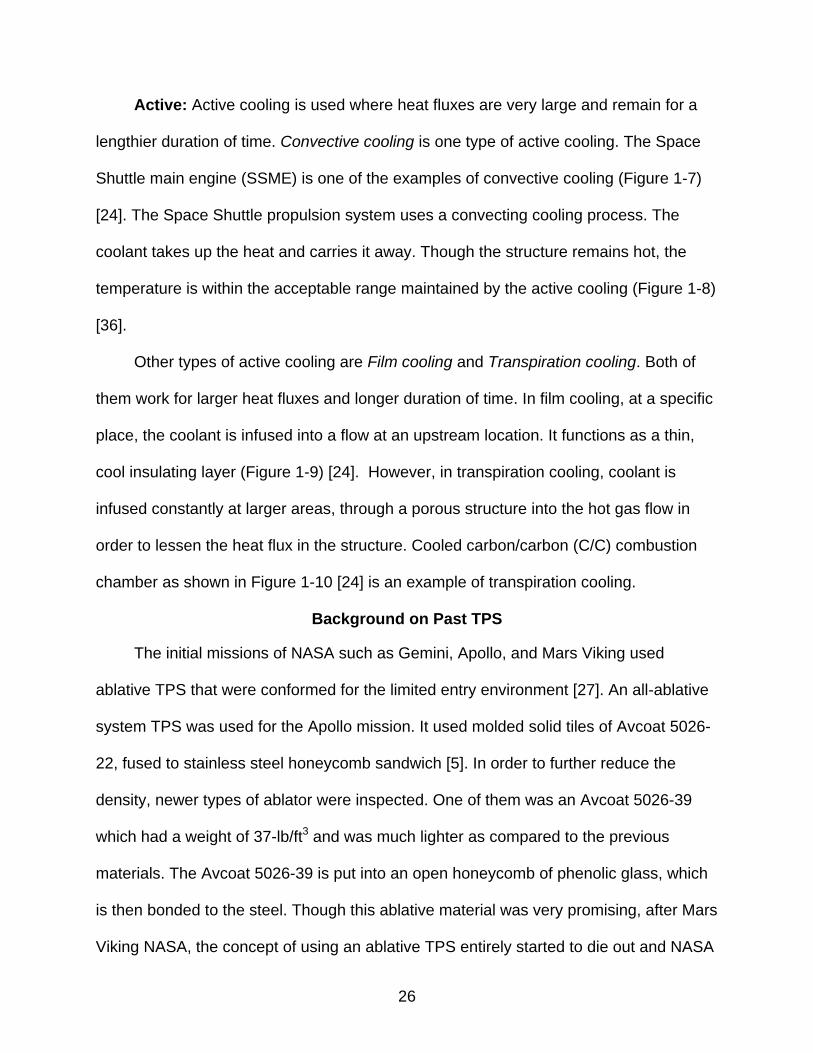
Active: Active cooling is used where heat fluxes are very large and remain for a
lengthier duration of time. Convective cooling is one type of active cooling. The Space
Shuttle main engine (SSME) is one of the examples of convective cooling (Figure 1-7)
[24]. The Space Shuttle propulsion system uses a convecting cooling process. The
coolant takes up the heat and carries it away. Though the structure remains hot, the
temperature is within the acceptable range maintained by the active cooling (Figure 1-8)
[36].
Other types of active cooling are Film cooling and Transpiration cooling. Both of
them work for larger heat fluxes and longer duration of time. In film cooling, at a specific
place, the coolant is infused into a flow at an upstream location. It functions as a thin,
cool insulating layer (Figure 1-9) [24]. However, in transpiration cooling, coolant is
infused constantly at larger areas, through a porous structure into the hot gas flow in
order to lessen the heat flux in the structure. Cooled carbon/carbon (C/C) combustion
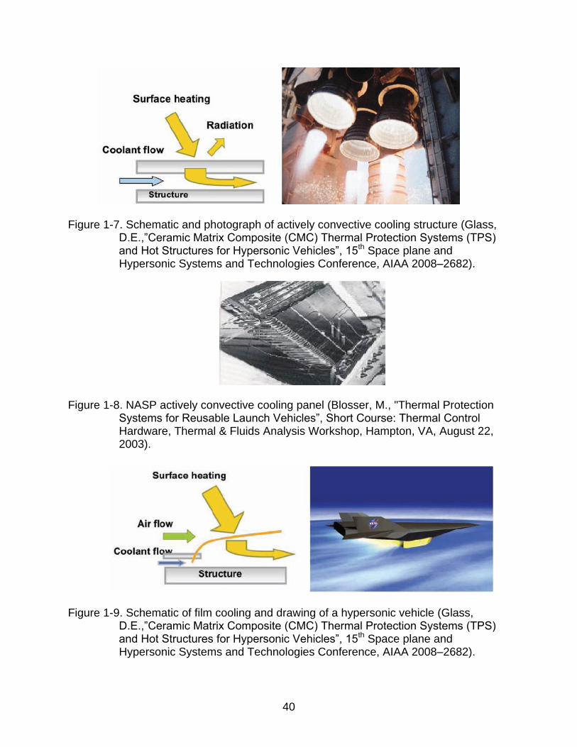
chamber as shown in Figure 1-10 [24] is an example of transpiration cooling.
Background on Past TPS
The initial missions of NASA such as Gemini, Apollo, and Mars Viking used
ablative TPS that were conformed for the limited entry environment [27]. An all-ablative
system TPS was used for the Apollo mission. It used molded solid tiles of Avcoat 5026-
22, fused to stainless steel honeycomb sandwich [5]. In order to further reduce the
density, newer types of ablator were inspected. One of them was an Avcoat 5026-39
which had a weight of 37-lb/ft3 and was much lighter as compared to the previous
materials. The Avcoat 5026-39 is put into an open honeycomb of phenolic glass, which
is then bonded to the steel. Though this ablative material was very promising, after Mars
Viking NASA, the concept of using an ablative TPS entirely started to die out and NASA
27
started moving the research towards reusable TPS in support of Space Shuttle. The
TPS is spread over approximately the whole orbiter surface, and it composes of eight
different materials in various places; based on the amount of heat shield it requires [29].
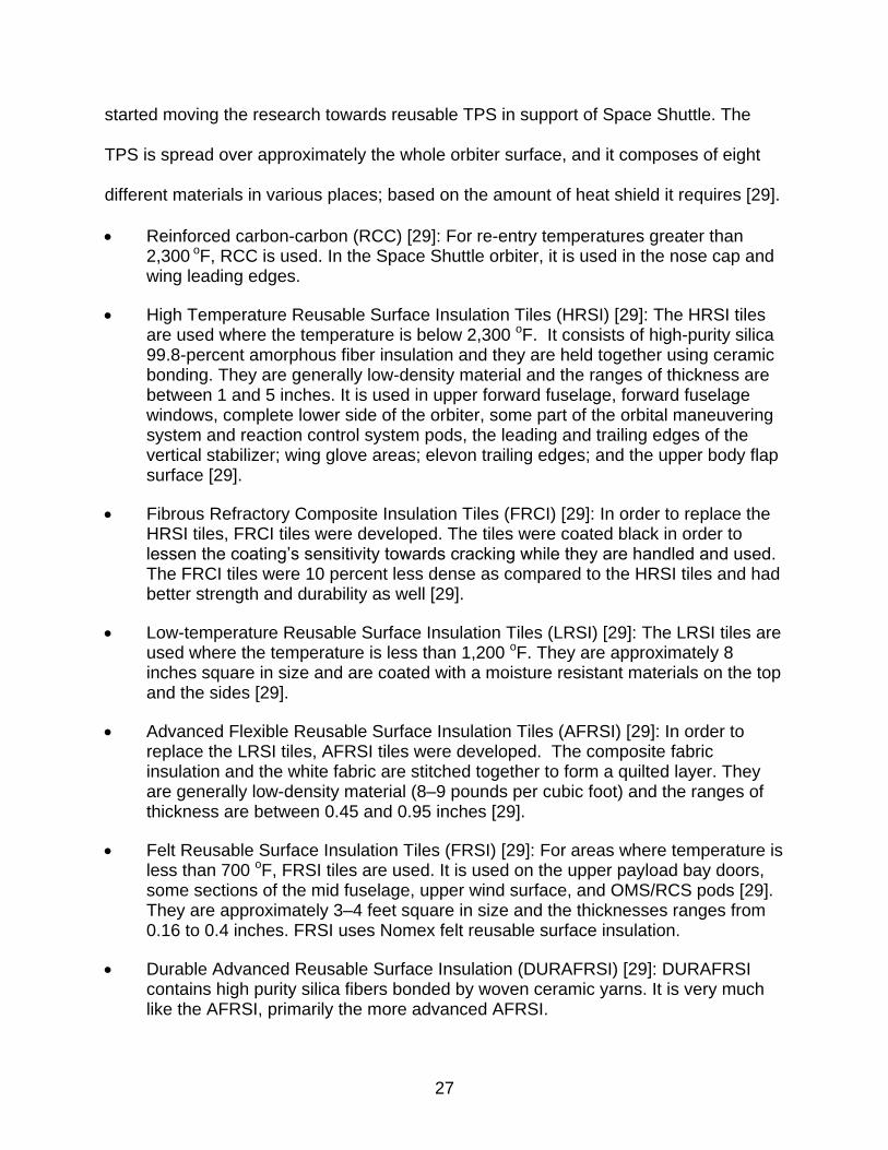
Reinforced carbon-carbon (RCC) [29]: For re-entry temperatures greater than 2,300 oF, RCC is used. In the Space Shuttle orbiter, it is used in the nose cap and wing leading edges.
High Temperature Reusable Surface Insulation Tiles (HRSI) [29]: The HRSI tiles are used where the temperature is below 2,300 oF. It consists of high-purity silica 99.8-percent amorphous fiber insulation and they are held together using ceramic bonding. They are generally low-density material and the ranges of thickness are between 1 and 5 inches. It is used in upper forward fuselage, forward fuselage windows, complete lower side of the orbiter, some part of the orbital maneuvering system and reaction control system pods, the leading and trailing edges of the vertical stabilizer; wing glove areas; elevon trailing edges; and the upper body flap surface [29].
Fibrous Refractory Composite Insulation Tiles (FRCI) [29]: In order to replace the HRSI tiles, FRCI tiles were developed. The tiles were coated black in order to lessen the coating‟s sensitivity towards cracking while they are handled and used. The FRCI tiles were 10 percent less dense as compared to the HRSI tiles and had better strength and durability as well [29].
Low-temperature Reusable Surface Insulation Tiles (LRSI) [29]: The LRSI tiles are used where the temperature is less than 1,200 oF. They are approximately 8 inches square in size and are coated with a moisture resistant materials on the top and the sides [29].
Advanced Flexible Reusable Surface Insulation Tiles (AFRSI) [29]: In order to replace the LRSI tiles, AFRSI tiles were developed. The composite fabric insulation and the white fabric are stitched together to form a quilted layer. They are generally low-density material (8–9 pounds per cubic foot) and the ranges of thickness are between 0.45 and 0.95 inches [29].
Felt Reusable Surface Insulation Tiles (FRSI) [29]: For areas where temperature is less than 700 oF, FRSI tiles are used. It is used on the upper payload bay doors, some sections of the mid fuselage, upper wind surface, and OMS/RCS pods [29]. They are approximately 3–4 feet square in size and the thicknesses ranges from 0.16 to 0.4 inches. FRSI uses Nomex felt reusable surface insulation.
Durable Advanced Reusable Surface Insulation (DURAFRSI) [29]: DURAFRSI contains high purity silica fibers bonded by woven ceramic yarns. It is very much like the AFRSI, primarily the more advanced AFRSI.
28
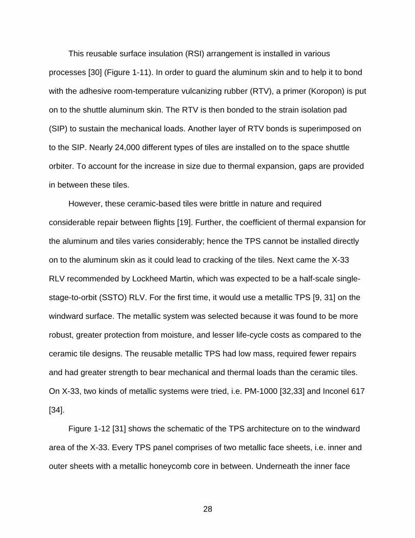
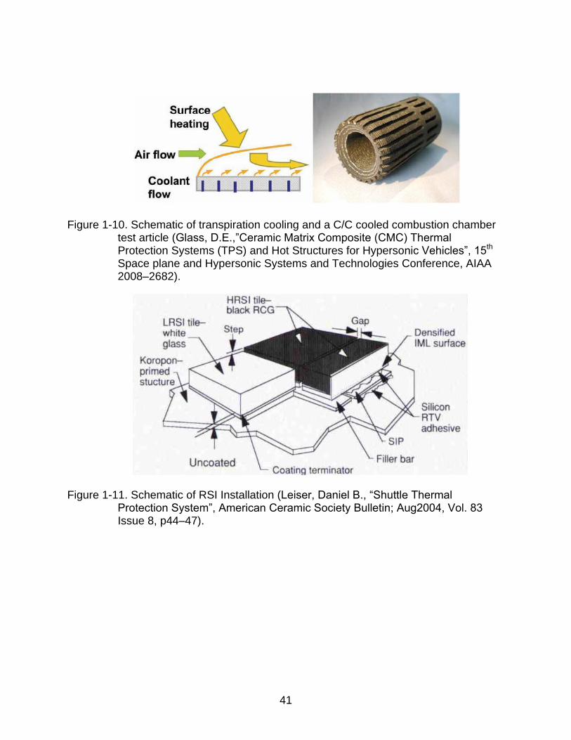
This reusable surface insulation (RSI) arrangement is installed in various
processes [30] (Figure 1-11). In order to guard the aluminum skin and to help it to bond
with the adhesive room-temperature vulcanizing rubber (RTV), a primer (Koropon) is put
on to the shuttle aluminum skin. The RTV is then bonded to the strain isolation pad
(SIP) to sustain the mechanical loads. Another layer of RTV bonds is superimposed on
to the SIP. Nearly 24,000 different types of tiles are installed on to the space shuttle
orbiter. To account for the increase in size due to thermal expansion, gaps are provided
in between these tiles.
However, these ceramic-based tiles were brittle in nature and required
considerable repair between flights [19]. Further, the coefficient of thermal expansion for
the aluminum and tiles varies considerably; hence the TPS cannot be installed directly
on to the aluminum skin as it could lead to cracking of the tiles. Next came the X-33
RLV recommended by Lockheed Martin, which was expected to be a half-scale single-
stage-to-orbit (SSTO) RLV. For the first time, it would use a metallic TPS [9, 31] on the
windward surface. The metallic system was selected because it was found to be more
robust, greater protection from moisture, and lesser life-cycle costs as compared to the
ceramic tile designs. The reusable metallic TPS had low mass, required fewer repairs
and had greater strength to bear mechanical and thermal loads than the ceramic tiles.
On X-33, two kinds of metallic systems were tried, i.e. PM-1000 [32,33] and Inconel 617
[34].
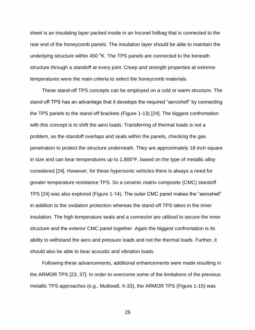
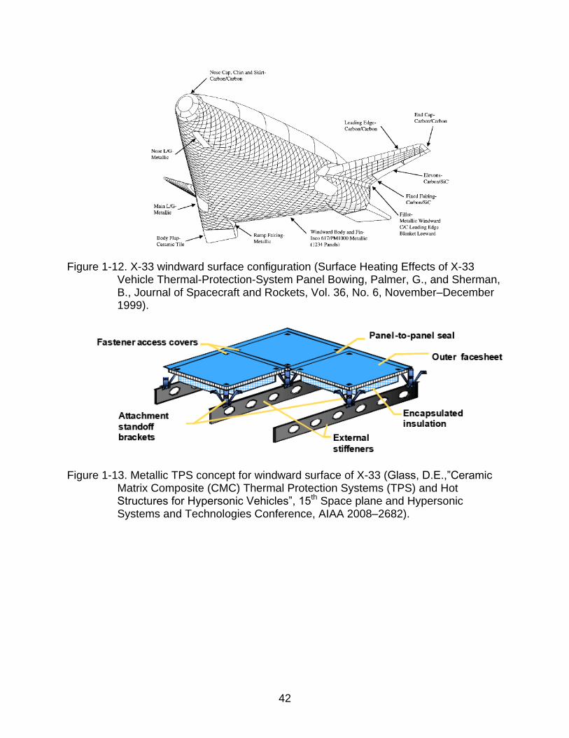
Figure 1-12 [31] shows the schematic of the TPS architecture on to the windward
area of the X-33. Every TPS panel comprises of two metallic face sheets, i.e. inner and
outer sheets with a metallic honeycomb core in between. Underneath the inner face
29
sheet is an insulating layer packed inside in an Inconel foilbag that is connected to the
rear end of the honeycomb panels. The insulation layer should be able to maintain the
underlying structure within 450 oK. The TPS panels are connected to the beneath
structure through a standoff at every joint. Creep and strength properties at extreme
temperatures were the main criteria to select the honeycomb materials.
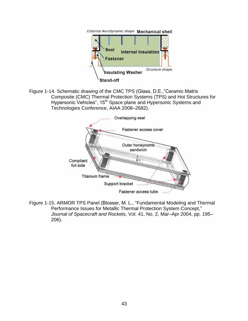
These stand-off TPS concepts can be employed on a cold or warm structure. The
stand-off TPS has an advantage that it develops the required “aeroshell” by connecting
the TPS panels to the stand-off brackets (Figure 1-13) [24]. The biggest confrontation
with this concept is to shift the aero loads. Transferring of thermal loads is not a
problem, as the standoff overlaps and seals within the panels, checking the gas
penetration to protect the structure underneath. They are approximately 18 inch square
in size and can bear temperatures up to 1,800°F, based on the type of metallic alloy
considered [24]. However, for these hypersonic vehicles there is always a need for
greater temperature resistance TPS. So a ceramic matrix composite (CMC) standoff
TPS [24] was also explored (Figure 1-14). The outer CMC panel makes the “aeroshell”
in addition to the oxidation protection whereas the stand-off TPS takes in the inner
insulation. The high temperature seals and a connector are utilized to secure the inner
structure and the exterior CMC panel together. Again the biggest confrontation is its
ability to withstand the aero and pressure loads and not the thermal loads. Further, it
should also be able to bear acoustic and vibration loads.
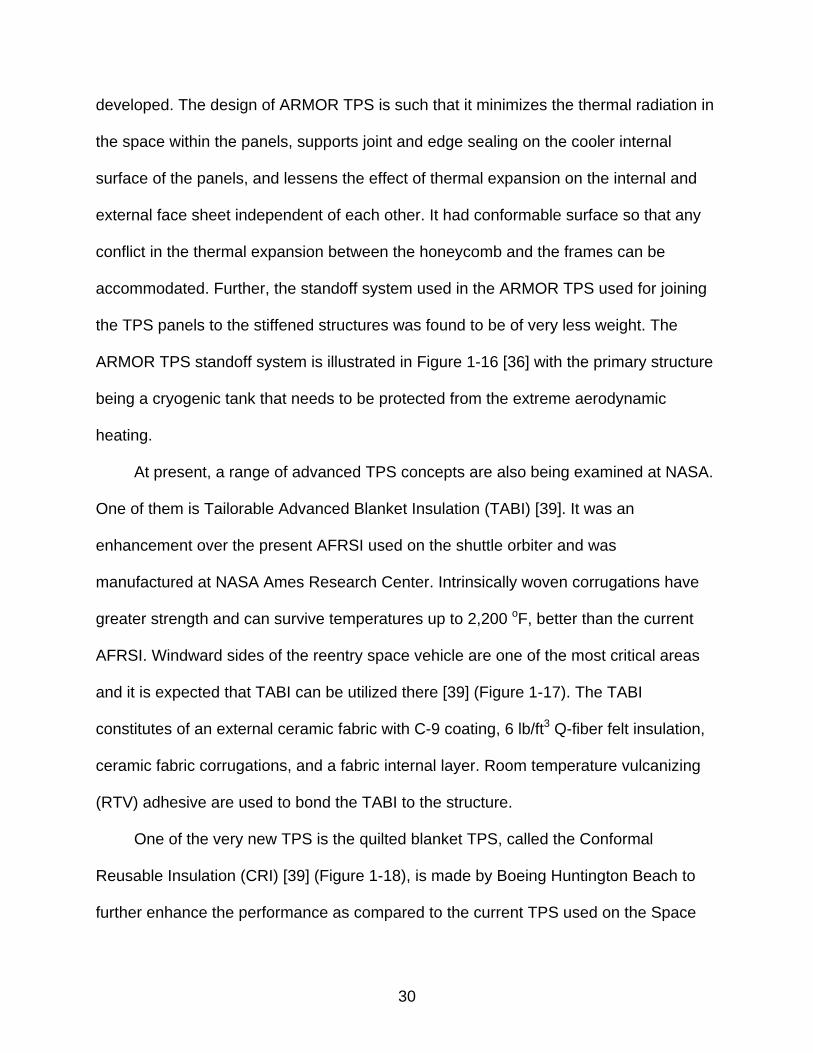
Following these advancements, additional enhancements were made resulting in
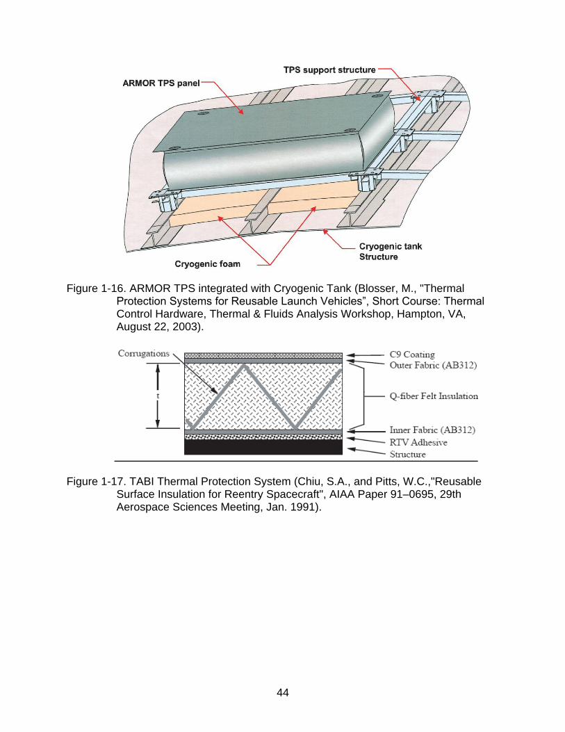
the ARMOR TPS [23, 37]. In order to overcome some of the limitations of the previous
metallic TPS approaches (e.g., Multiwall, X-33), the ARMOR TPS (Figure 1-15) was
30
developed. The design of ARMOR TPS is such that it minimizes the thermal radiation in
the space within the panels, supports joint and edge sealing on the cooler internal
surface of the panels, and lessens the effect of thermal expansion on the internal and
external face sheet independent of each other. It had conformable surface so that any
conflict in the thermal expansion between the honeycomb and the frames can be
accommodated. Further, the standoff system used in the ARMOR TPS used for joining
the TPS panels to the stiffened structures was found to be of very less weight. The
ARMOR TPS standoff system is illustrated in Figure 1-16 [36] with the primary structure
being a cryogenic tank that needs to be protected from the extreme aerodynamic
heating.
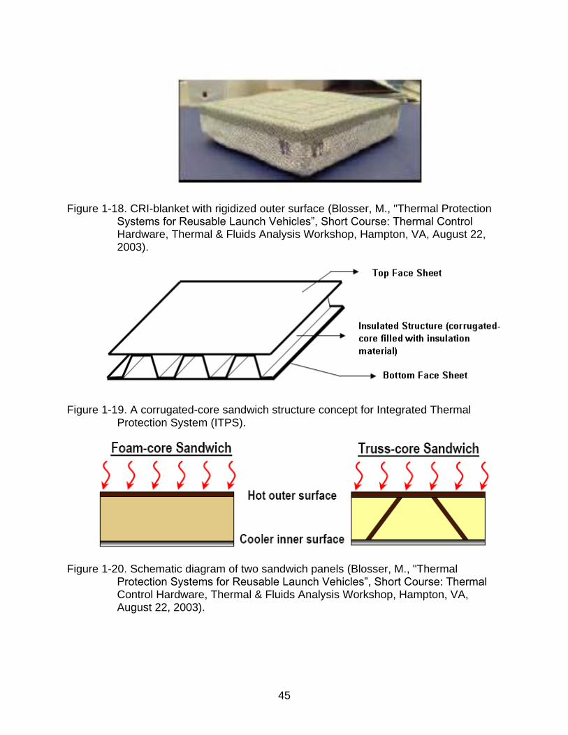
At present, a range of advanced TPS concepts are also being examined at NASA.
One of them is Tailorable Advanced Blanket Insulation (TABI) [39]. It was an
enhancement over the present AFRSI used on the shuttle orbiter and was
manufactured at NASA Ames Research Center. Intrinsically woven corrugations have
greater strength and can survive temperatures up to 2,200 oF, better than the current
AFRSI. Windward sides of the reentry space vehicle are one of the most critical areas
and it is expected that TABI can be utilized there [39] (Figure 1-17). The TABI
constitutes of an external ceramic fabric with C-9 coating, 6 lb/ft3 Q-fiber felt insulation,
ceramic fabric corrugations, and a fabric internal layer. Room temperature vulcanizing
(RTV) adhesive are used to bond the TABI to the structure.
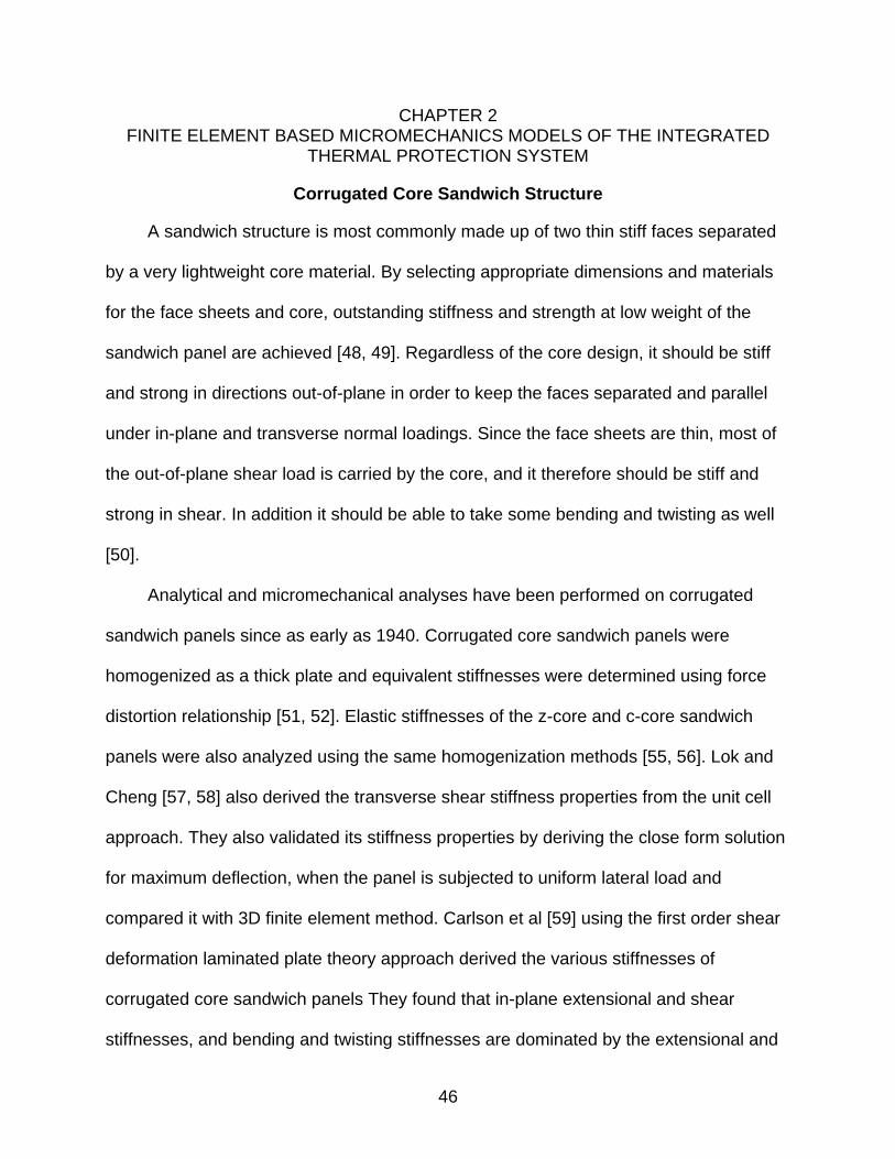
One of the very new TPS is the quilted blanket TPS, called the Conformal
Reusable Insulation (CRI) [39] (Figure 1-18), is made by Boeing Huntington Beach to
further enhance the performance as compared to the current TPS used on the Space
31
Shuttle orbiter. Based on the matrix composition used on the CRI, the temperature limit
can vary from 1,800°F-2000°F. The CRI is manufactured using a unique method by
putting the ceramic batting material in between the ceramic fiber face sheets and this
“rigidization” approach significantly improves the fabrication of CRI, with perfectly flat
blankets and excellent dimensional precision.
The latest spacecraft thermal protection systems are the Boeing Rigid Insulation
(BRI) and Alumina Enhanced Thermal Barrier (AETB) ceramic tile with Toughened Uni-
Piece Fibrous Insulation (TUFI) coating [40], which have a very high operational
temperature. AETB was manufactured at the Ames Research Center and it has
excellent strength and durability. It can protect areas where temperatures are as high as
2,500 oF. The AETB ceramic tiles are approximately 8 inches square in size and are
coated with TUFI. Strain isolation pads (SIPs) are used between the AETB tiles and the
substructure to compensate for the thermal expansion mismatch between the two.
Integral Thermal Protection System
With the recent emphasis on commercial RLV‟s, reducing TPS cost has become
an increasingly important consideration. The costs for development, fabrication,
installation, fuel required to carry it and maintenance all contribute to the total life-cycle
cost. Reduced life cycle costs imply design drivers such as robustness and operability
to lower maintenance costs. A robust TPS is not easily damaged by its design
environment and may be able to tolerate some damage without requiring immediate
repair. An operable TPS should be easily inspected, removed and replaced, maintained,
and repaired if necessary. Low maintenance is especially important for RLV‟s for which
rapid turnaround is critical to economic viability.
32
In particular, weight of the TPS is one of the most important design criteria, as
TPS occupies huge area on the vehicle surface and thus a huge factor for cost. Low
mass is important for TPS, carried by a high speed vehicle which must be accelerated
and/or decelerated through large changes in velocity. The energy to accelerate
additional TPS mass requires additional fuel, and a larger vehicle to contain that fuel, or
a reduction in payload mass. Consequently, TPS designs are primarily performance
driven, that is, designed for minimum mass to perform the thermal function. The
substructure beneath the TPS bears all the mechanical loads. Further, due to the brittle
nature and low strength of tiles, ceramic tile TPS must be isolated from the mechanical
strains of the underlying sub structure. This is accomplished by the felt strain isolation
pad (SIP). Thus, the TPS was used as an add-on to the structure of the hypersonic
vehicle. Further, the tiles have been susceptible to impact damage, and have required
waterproofing after each flight. Inspections, repairs, and waterproofing are time-
consuming and costly.
These add-on concepts had many other problems. One of them is the
incompatibility of the load bearing structure and the TPS, thereby compromising the
strength of the surface of the space vehicle. The tiles may not bond really well with the
structure, which could result in slackening and separation of tiles from the structure and
thereby causing catastrophic failure of the space vehicle. The newer TPS approaches
like the BRI and AETB also overcome some of the limitations of the add-on TPS
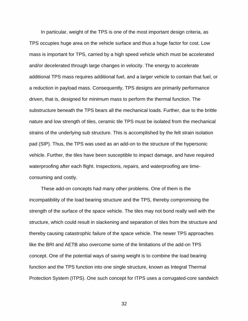
concept. One of the potential ways of saving weight is to combine the load bearing
function and the TPS function into one single structure, known as Integral Thermal
Protection System (ITPS). One such concept for ITPS uses a corrugated-core sandwich
33
structure. An ITPS is a sandwich panel composed of two thin faces separated by a
corrugated core structure which can be of homogeneous materials such as metals or
orthotropic materials such as composite laminates. The two thin faces are the top face
sheet (TFS) and the bottom face sheet (BFS) with a corrugated web in between (Figure
1-19). The sandwich panel is composed of several unit cells placed adjacent to each
other. The empty space in the corrugated core will be filled with a non load-bearing
insulation such as Safill®. It combines the three passive TPS concepts of hot structure,
insulated structure and heat sink. The outer and inner walls of ITPS carry the airframe
loads, with the outer wall operating hot and the inner wall insulated. It is thermally
integrated, has a higher structural efficiency, and is potentially lower maintenance. The
outer surface is a robust, high-temperature material. The wall thickness helps provide
stiffness and the large integrated structure eliminates/reduces surface gaps and steps.
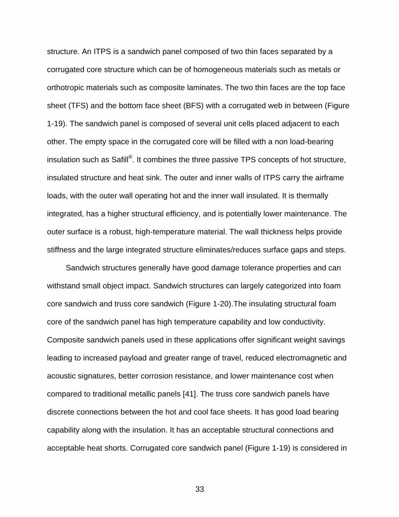
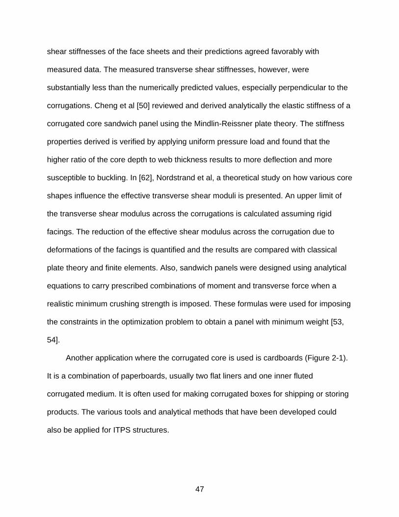
Sandwich structures generally have good damage tolerance properties and can
withstand small object impact. Sandwich structures can largely categorized into foam
core sandwich and truss core sandwich (Figure 1-20).The insulating structural foam
core of the sandwich panel has high temperature capability and low conductivity.
Composite sandwich panels used in these applications offer significant weight savings
leading to increased payload and greater range of travel, reduced electromagnetic and
acoustic signatures, better corrosion resistance, and lower maintenance cost when
compared to traditional metallic panels [41]. The truss core sandwich panels have
discrete connections between the hot and cool face sheets. It has good load bearing
capability along with the insulation. It has an acceptable structural connections and
acceptable heat shorts. Corrugated core sandwich panel (Figure 1-19) is considered in
34
the present study. Other truss core sandwich panels are also being investigated by
other research groups. The core geometries analyzed were truss-cores with tetragonal,
pyramidal, and kagome configurations [42, 43, 44] and prismatic cores with corrugated
and diamond (or textile) configurations [45, 46, 47]. In all of these panels bending,
transverse shear and crushing loads were considered for analysis. However, the
heights of these sandwich panels were approximately 20 to 30 mm which were very
small as compared to the ITPS panels (70–90 mm) because TPS dictates that the
height be as large as possible to increase the heat conduction path.
The biggest challenge of an ITPS is that the requirements of a load-bearing
member and a TPS are contradictory to one another. A TPS is required to have low
conductivity and high service temperatures. Materials satisfying these conditions are
ceramic materials, which are also plagued by poor structural properties like low impact
resistance, low tensile strength and low fracture toughness. On the other hand, a robust
load-bearing structure needs to have high tensile strength and fracture toughness and
good impact resistance. Materials that satisfy these requirements are metals and
metallic alloys, which have relatively high conductivity and low service temperatures.
The challenge is to combine these functions into one structure satisfying all the required
constraints.
The top face sheet is a hot structure and ceramic composites such as SiC/SiC
composites and titanium alloys (Ti-6Al-4V) are candidate materials. The web could also
be made of similar composite. From weight efficiency point of view the bottom face
sheet is expected to be a heat sink for the ITPS; therefore a material that has a high
heat capacity is needed for the bottom face sheet. The bottom face sheet will also
35
experience a major portion of the in-plane stresses because of the attachment
mechanisms of stringers and frames to the space vehicle. Therefore, a high Young‟s
Modulus material with a high heat capacity is suitable for the bottom face sheet. Thus
there are several design variables - geometric and material property variables. The
design of such a TPS will require several thousand analyses to obtain a minimum mass
design. When the uncertainties in properties, dimensions and loads are taken into
account, the computational costs will be prohibitively high. Hence, there is a need to
develop efficient methods for analysis and design of ITPS for future space vehicles.
Dissertation Organization or Outline
The objectives of this research are:
Develop a finite element analysis based homogenization method to model the composite ITPS as a homogeneous orthotropic plate.
Perform simulations on the 2D plate model to obtain responses such as stresses and displacements as a function of the design variables to create 2D response surfaces (2D-RS).
Develop a simplified buckling analysis and compare it with the 3D buckling analysis to create a 2D response surfaces.
Develop correction response surface using algebraic surrogates (CRS).
Develop a multi-fidelity analysis to compute the response variables to optimize the design.
The chapters are organized as follows. In Chapter 2, a finite element (FE) based
micromechanical analysis procedure is developed for modeling corrugated sandwich
panels as 2D orthotropic plates. The equivalent stiffness parameters such as the
extensional, bending, coupling and shear stiffnesses of the ITPS are obtained. These
parameters are input into 2D FE plate model. In Chapter 3, a FE based homogenization
and reverse homogenization procedure is described. The equivalent plate responses
36
such as the stresses and displacements are obtained, when subjected to thermal and
pressure loads. The plate responses are also compared with the corresponding 3D
analysis. In Chapter 4, the key design drivers of the ITPS are identified. The ITPS is
optimized for a minimum mass design while satisfying all of the constraints. The
constraints are generated using a response surface. Different types of response
surfaces are explored and based on the error of the fit; the best response surface is
used. Finally, in Chapter 5, an overview of this dissertation research and findings are
presented.
37
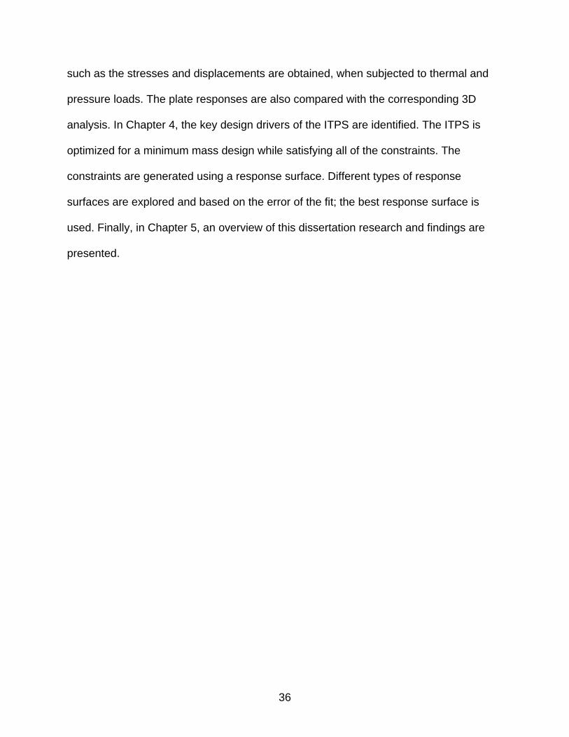
Figure 1-1. Space Shuttle photograph showing release point of 1.7-lb foam at the bipod ramp and the impact point on the left wing leading edge (Lyle, K.H., & Fasanella, E.L., "Permanent set of the Space Shuttle Thermal Protection System Reinforced Carbon–Carbon material",Journal of Composites, Part A 40 (2009) 702–708).
Figure 1-2. Schematic and photograph (Space Shuttle Orbiter elevons) of an insulated structure (Glass, D.E.,”Ceramic Matrix Composite (CMC) Thermal Protection Systems (TPS) and Hot Structures for Hypersonic Vehicles”, 15th Space plane and Hypersonic Systems and Technologies Conference, AIAA 2008–2682).
38
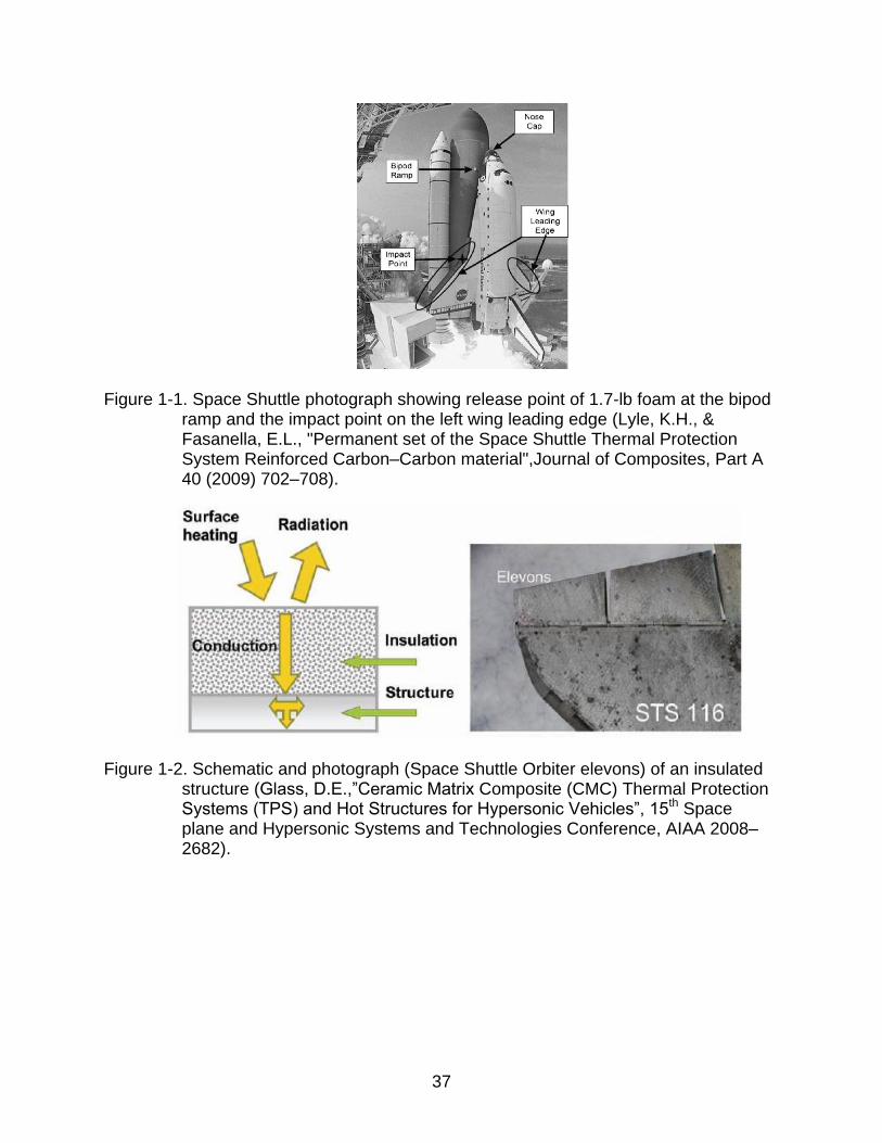
Figure 1-3. Schematic and photograph (X-15) of a heat sink structure (Glass, D.E.,”Ceramic Matrix Composite (CMC) Thermal Protection Systems (TPS) and Hot Structures for Hypersonic Vehicles”, 15th Space plane and Hypersonic Systems and Technologies Conference, AIAA 2008–2682).
Figure 1-4. Schematic and photograph of a hot structure (Glass, D.E.,”Ceramic Matrix Composite (CMC) Thermal Protection Systems (TPS) and Hot Structures for Hypersonic Vehicles”, 15th Space plane and Hypersonic Systems and Technologies Conference, AIAA 2008–2682).
39
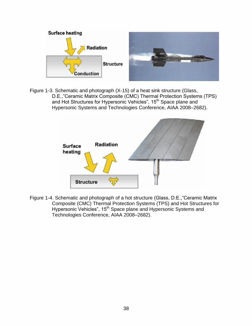
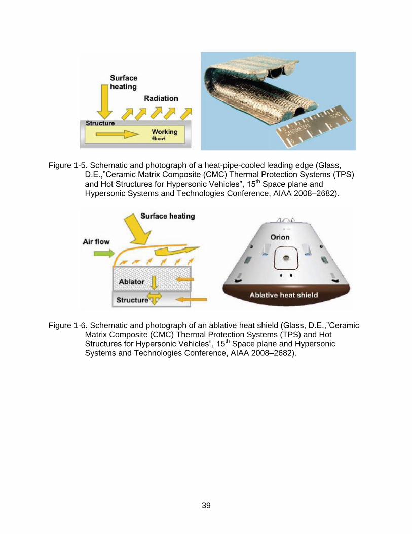
Figure 1-5. Schematic and photograph of a heat-pipe-cooled leading edge (Glass, D.E.,”Ceramic Matrix Composite (CMC) Thermal Protection Systems (TPS) and Hot Structures for Hypersonic Vehicles”, 15th Space plane and Hypersonic Systems and Technologies Conference, AIAA 2008–2682).
Figure 1-6. Schematic and photograph of an ablative heat shield (Glass, D.E.,”Ceramic Matrix Composite (CMC) Thermal Protection Systems (TPS) and Hot Structures for Hypersonic Vehicles”, 15th Space plane and Hypersonic Systems and Technologies Conference, AIAA 2008–2682).
40
Figure 1-7. Schematic and photograph of actively convective cooling structure (Glass, D.E.,”Ceramic Matrix Composite (CMC) Thermal Protection Systems (TPS) and Hot Structures for Hypersonic Vehicles”, 15th Space plane and Hypersonic Systems and Technologies Conference, AIAA 2008–2682).
Figure 1-8. NASP actively convective cooling panel (Blosser, M., "Thermal Protection Systems for Reusable Launch Vehicles”, Short Course: Thermal Control Hardware, Thermal & Fluids Analysis Workshop, Hampton, VA, August 22, 2003).
Figure 1-9. Schematic of film cooling and drawing of a hypersonic vehicle (Glass, D.E.,”Ceramic Matrix Composite (CMC) Thermal Protection Systems (TPS) and Hot Structures for Hypersonic Vehicles”, 15th Space plane and Hypersonic Systems and Technologies Conference, AIAA 2008–2682).
41
Figure 1-10. Schematic of transpiration cooling and a C/C cooled combustion chamber test article (Glass, D.E.,”Ceramic Matrix Composite (CMC) Thermal Protection Systems (TPS) and Hot Structures for Hypersonic Vehicles”, 15th Space plane and Hypersonic Systems and Technologies Conference, AIAA 2008–2682).
Figure 1-11. Schematic of RSI Installation (Leiser, Daniel B., “Shuttle Thermal Protection System”, American Ceramic Society Bulletin; Aug2004, Vol. 83 Issue 8, p44–47).
42
Figure 1-12. X-33 windward surface configuration (Surface Heating Effects of X-33 Vehicle Thermal-Protection-System Panel Bowing, Palmer, G., and Sherman, B., Journal of Spacecraft and Rockets, Vol. 36, No. 6, November–December 1999).
Figure 1-13. Metallic TPS concept for windward surface of X-33 (Glass, D.E.,”Ceramic Matrix Composite (CMC) Thermal Protection Systems (TPS) and Hot Structures for Hypersonic Vehicles”, 15th Space plane and Hypersonic Systems and Technologies Conference, AIAA 2008–2682).
43
Figure 1-14. Schematic drawing of the CMC TPS (Glass, D.E.,”Ceramic Matrix Composite (CMC) Thermal Protection Systems (TPS) and Hot Structures for Hypersonic Vehicles”, 15th Space plane and Hypersonic Systems and Technologies Conference, AIAA 2008–2682).
Figure 1-15. ARMOR TPS Panel (Blosser, M. L., “Fundamental Modeling and Thermal Performance Issues for Metallic Thermal Protection System Concept,” Journal of Spacecraft and Rockets, Vol. 41, No. 2, Mar–Apr 2004, pp. 195–206).
44
Figure 1-16. ARMOR TPS integrated with Cryogenic Tank (Blosser, M., "Thermal Protection Systems for Reusable Launch Vehicles”, Short Course: Thermal Control Hardware, Thermal & Fluids Analysis Workshop, Hampton, VA, August 22, 2003).
Figure 1-17. TABI Thermal Protection System (Chiu, S.A., and Pitts, W.C.,"Reusable Surface Insulation for Reentry Spacecraft", AIAA Paper 91–0695, 29th Aerospace Sciences Meeting, Jan. 1991).
45
Figure 1-18. CRI-blanket with rigidized outer surface (Blosser, M., "Thermal Protection Systems for Reusable Launch Vehicles”, Short Course: Thermal Control Hardware, Thermal & Fluids Analysis Workshop, Hampton, VA, August 22, 2003).
Figure 1-19. A corrugated-core sandwich structure concept for Integrated Thermal Protection System (ITPS).
Figure 1-20. Schematic diagram of two sandwich panels (Blosser, M., "Thermal Protection Systems for Reusable Launch Vehicles”, Short Course: Thermal Control Hardware, Thermal & Fluids Analysis Workshop, Hampton, VA, August 22, 2003).
46
CHAPTER 2 FINITE ELEMENT BASED MICROMECHANICS MODELS OF THE INTEGRATED
THERMAL PROTECTION SYSTEM
Corrugated Core Sandwich Structure
A sandwich structure is most commonly made up of two thin stiff faces separated
by a very lightweight core material. By selecting appropriate dimensions and materials
for the face sheets and core, outstanding stiffness and strength at low weight of the
sandwich panel are achieved [48, 49]. Regardless of the core design, it should be stiff
and strong in directions out-of-plane in order to keep the faces separated and parallel
under in-plane and transverse normal loadings. Since the face sheets are thin, most of
the out-of-plane shear load is carried by the core, and it therefore should be stiff and
strong in shear. In addition it should be able to take some bending and twisting as well
[50].
Analytical and micromechanical analyses have been performed on corrugated
sandwich panels since as early as 1940. Corrugated core sandwich panels were
homogenized as a thick plate and equivalent stiffnesses were determined using force
distortion relationship [51, 52]. Elastic stiffnesses of the z-core and c-core sandwich
panels were also analyzed using the same homogenization methods [55, 56]. Lok and
Cheng [57, 58] also derived the transverse shear stiffness properties from the unit cell
approach. They also validated its stiffness properties by deriving the close form solution
for maximum deflection, when the panel is subjected to uniform lateral load and
compared it with 3D finite element method. Carlson et al [59] using the first order shear
deformation laminated plate theory approach derived the various stiffnesses of
corrugated core sandwich panels They found that in-plane extensional and shear
stiffnesses, and bending and twisting stiffnesses are dominated by the extensional and
47
shear stiffnesses of the face sheets and their predictions agreed favorably with
measured data. The measured transverse shear stiffnesses, however, were
substantially less than the numerically predicted values, especially perpendicular to the
corrugations. Cheng et al [50] reviewed and derived analytically the elastic stiffness of a
corrugated core sandwich panel using the Mindlin-Reissner plate theory. The stiffness
properties derived is verified by applying uniform pressure load and found that the
higher ratio of the core depth to web thickness results to more deflection and more
susceptible to buckling. In [62], Nordstrand et al, a theoretical study on how various core
shapes influence the effective transverse shear moduli is presented. An upper limit of
the transverse shear modulus across the corrugations is calculated assuming rigid
facings. The reduction of the effective shear modulus across the corrugation due to
deformations of the facings is quantified and the results are compared with classical
plate theory and finite elements. Also, sandwich panels were designed using analytical
equations to carry prescribed combinations of moment and transverse force when a
realistic minimum crushing strength is imposed. These formulas were used for imposing
the constraints in the optimization problem to obtain a panel with minimum weight [53,
54].
Another application where the corrugated core is used is cardboards (Figure 2-1).
It is a combination of paperboards, usually two flat liners and one inner fluted
corrugated medium. It is often used for making corrugated boxes for shipping or storing
products. The various tools and analytical methods that have been developed could
also be applied for ITPS structures.
48
Biancolini [60] derived the equivalent stiffness properties of corrugated boards by
performing static condensation of the stiffness matrix obtained using the finite element
model of the full panel. Buannic et al. [61] used asymptotic expansion based analytical
method for deriving the equivalent properties of corrugated panel. Talbi, Batti et al [63],
has developed the equivalent stiffness of the analytical homogenization model for
corrugated cardboard and numerically implemented using a 3-node shell element. They
also compared the results with 3D model under different types of loading like tension,
compression, bending, transverse shear, in plane shear and torsion. In Isakasson et al
[64], the corrugated board panel is divided into an arbitrary number of thin virtual layers.
For each virtual layer, a unique effective elastic modulus is calculated. Then, the elastic
properties in all layers are assembled together in order to analyze a corrugated board
as a continuous structure having equivalent mechanical properties to a real structure. It
uses the strain energy approach to calculate the effective modulus for a corrugated
core. Also assuming that the transverse shear strain will vary through the plate
thickness, they developed an analytical expression for shear correction factors using the
energy approach. The capability of the model to properly capture and simulate the
mechanical behavior of corrugated boards subjected to plate bending as well as three-
point-bending has been demonstrated and are also compared to experiments on
corrugated board panels of varying geometry. Martinez et al [65, 66] uses a strain
energy approach and a transformation deformation matrix to determine analytically the
equivalent stiffness matrix of the sandwich panel.
49
Geometric Variables and Material Properties
The geometry of the ITPS structure with corrugated-core design is shown in Figure
2-2. This geometry can be completely described using the following 6 geometric
variables:
Thickness of top face sheet (TFS), tTF.
Thickness of webs, tW.
Thickness of bottom face sheet (BFS), tBF.
Angle of corrugations, θ.
Height of the sandwich panel (center-to-center distance between top and bottom face sheets), d.
Length of a unit-cell of the panel, 2p.
Unit Cell Analysis
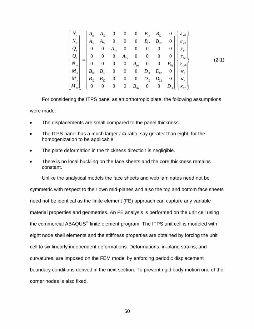
Micromechanical finite element analysis of a unit cell was performed to determine
the extensional, bending, coupling and transverse shear stiffness of the equivalent
orthotropic plate. This would require the prediction of the effective (macroscopic)
properties of the panel from its constituent (microscopic) components-the top face
sheet, bottom face sheets and the webs. The relationship between the unit cell macro
stresses and macro strains provided the constitutive relations for the material. Thus, the
in-plane extensional and shear response and out-of-plane (transverse) shear response
of an orthotropic panel are governed by the following constitutive relation:
50
011 12 11 12
012 22 12 22
44
55
066 66
11 12 11 12
12 22 12 22
66 66
0 0 0 0
0 0 0 0
0 0 0 0 0 0 0
0 0 0 0 0 0 0
0 0 0 0 0 0
0 0 0 0
0 0 0 0
0 0 0 0 0 0
x x
y y
y yz
x xz
xy xy
x x
y y
xy
N A A B B
N A A B B
Q A
Q A
N A B
M B B D D
M B B D D
M B D
xy
(2-1)
For considering the ITPS panel as an orthotropic plate, the following assumptions
were made:
The displacements are small compared to the panel thickness.
The ITPS panel has a much larger L/d ratio, say greater than eight, for the homogenization to be applicable.
The plate deformation in the thickness direction is negligible.
There is no local buckling on the face sheets and the core thickness remains constant.
Unlike the analytical models the face sheets and web laminates need not be
symmetric with respect to their own mid-planes and also the top and bottom face sheets
need not be identical as the finite element (FE) approach can capture any variable
material properties and geometries. An FE analysis is performed on the unit cell using
the commercial ABAQUS® finite element program. The ITPS unit cell is modeled with
eight node shell elements and the stiffness properties are obtained by forcing the unit
cell to six linearly independent deformations. Deformations, in-plane strains, and
curvatures, are imposed on the FEM model by enforcing periodic displacement
boundary conditions derived in the next section. To prevent rigid body motion one of the
corner nodes is also fixed.

51
Periodic Boundary Conditions
For the derivation of periodic boundary condition, we will consider the
displacement field ( , , ), ( , , )and ( , , )u x y z v x y z w x y z within the unit cell, which is a
hexahedron of size a×b×h. Our goal is to determine a set of boundary conditions (BCs)
that need to be applied on the surfaces of the unit cell such that the average
deformation in the unit cell is equal to a given value. There are infinite sets of BCs for a
given average strain. However, when the condition of periodicity is imposed, the
periodic BCs become almost unique. Before we derive the periodic BCs for various
average deformations, there are few assumptions which are used in the derivation.
They are as follows:
Materials are homogeneous and orthotropic.
Plate is assumed to be in the xy-plane with unit cells repeating in the x and y directions (Figure 2-3).
The plate is subjected to a uniform state of strain in the macroscopic sense (Figure 2-3).
All unit cells have identical stress and strain fields in micro scale. For the continuity of micro stresses across the unit cell it is required that tractions are equal and opposite at corresponding points on opposite faces of the unit cell.
For the derivation it is worth noting that the various unit cells must undergo
identical deformations. This requires that the deformed surface S+x - the surface normal
to the positive x direction - should be obtained by translating and rotating the deformed
surface S-x (Figure 2-4). Then one can write:
1 1
2 2
3 2
( , , ) (0, , )
( , , ) (0, , )
( , , ) (0, , )
u a y z u y z C R z
v a y z v y z C R z
w a y z w y z C R y
(2-2)
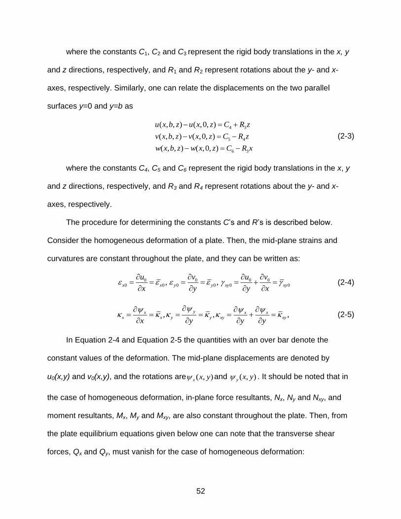
52
where the constants C1, C2 and C3 represent the rigid body translations in the x, y
and z directions, respectively, and R1 and R2 represent rotations about the y- and x-
axes, respectively. Similarly, one can relate the displacements on the two parallel
surfaces y=0 and y=b as
4 3
5 4
6 3
( , , ) ( ,0, )
( , , ) ( ,0, )
( , , ) ( ,0, )
u x b z u x z C R z
v x b z v x z C R z
w x b z w x z C R x
(2-3)
where the constants C4, C5 and C6 represent the rigid body translations in the x, y
and z directions, respectively, and R3 and R4 represent rotations about the y- and x-
axes, respectively.
The procedure for determining the constants C‟s and R‟s is described below.
Consider the homogeneous deformation of a plate. Then, the mid-plane strains and
curvatures are constant throughout the plate, and they can be written as:
0 0 0 00 0 0 0 0 0, ,x x y y xy xy
u v u v
x y y x
(2-4)
, , ,yx x x
x x y y xy xyx y y y
(2-5)
In Equation 2-4 and Equation 2-5 the quantities with an over bar denote the
constant values of the deformation. The mid-plane displacements are denoted by
u0(x,y) and v0(x,y), and the rotations are ( , )x x y and ( , )y x y . It should be noted that in
the case of homogeneous deformation, in-plane force resultants, Nx, Ny and Nxy, and
moment resultants, Mx, My and Mxy, are also constant throughout the plate. Then, from
the plate equilibrium equations given below one can note that the transverse shear
forces, Qx and Qy, must vanish for the case of homogeneous deformation:
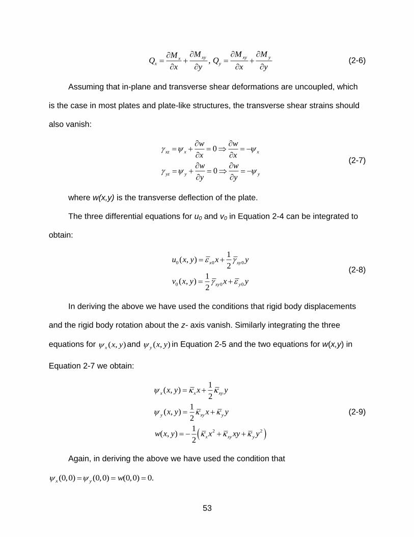
53
,xy xy yx
x y
M M MMQ Q
x y x y
(2-6)
Assuming that in-plane and transverse shear deformations are uncoupled, which
is the case in most plates and plate-like structures, the transverse shear strains should
also vanish:
0
0
xz x x
yz y y
w w
x x
w w
y y
(2-7)
where w(x,y) is the transverse deflection of the plate.
The three differential equations for u0 and v0 in Equation 2-4 can be integrated to
obtain:
0 0 0
0 0 0
1( , )
2
1( , )
2
x xy
xy y
u x y x y
v x y x y
(2-8)
In deriving the above we have used the conditions that rigid body displacements
and the rigid body rotation about the z- axis vanish. Similarly integrating the three
equations for ( , )x x y and ( , )y x y in Equation 2-5 and the two equations for w(x,y) in
Equation 2-7 we obtain:
2 2
1( , )
2
1( , )
2
1( , )
2
x x xy
y xy y
x xy y
x y x y
x y x y
w x y x xy y
(2-9)
Again, in deriving the above we have used the condition that
(0,0) (0,0) (0,0) 0.x y w
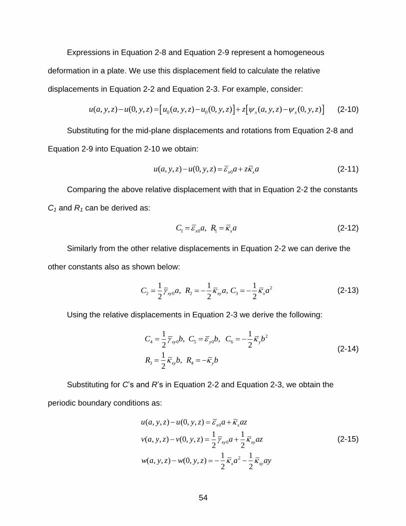
54
Expressions in Equation 2-8 and Equation 2-9 represent a homogeneous
deformation in a plate. We use this displacement field to calculate the relative
displacements in Equation 2-2 and Equation 2-3. For example, consider:
0 0( , , ) (0, , ) ( , , ) (0, , ) ( , , ) (0, , )x xu a y z u y z u a y z u y z z a y z y z (2-10)
Substituting for the mid-plane displacements and rotations from Equation 2-8 and
Equation 2-9 into Equation 2-10 we obtain:
0( , , ) (0, , ) x xu a y z u y z a z a (2-11)
Comparing the above relative displacement with that in Equation 2-2 the constants
C1 and R1 can be derived as:
1 0 1,x xC a R a (2-12)
Similarly from the other relative displacements in Equation 2-2 we can derive the
other constants also as shown below:
2
2 0 2 3
1 1 1, ,
2 2 2xy xy xC a R a C a (2-13)
Using the relative displacements in Equation 2-3 we derive the following:
2
4 0 5 0 6
3 4
1 1, ,
2 2
1,
2
xy y y
xy y
C b C b C b
R b R b
(2-14)
Substituting for C‟s and R‟s in Equation 2-2 and Equation 2-3, we obtain the
periodic boundary conditions as:
0
0
2
( , , ) (0, , )
1 1( , , ) (0, , )
2 2
1 1( , , ) (0, , )
2 2
x x
xy xy
x xy
u a y z u y z a az
v a y z v y z a az
w a y z w y z a ay
(2-15)
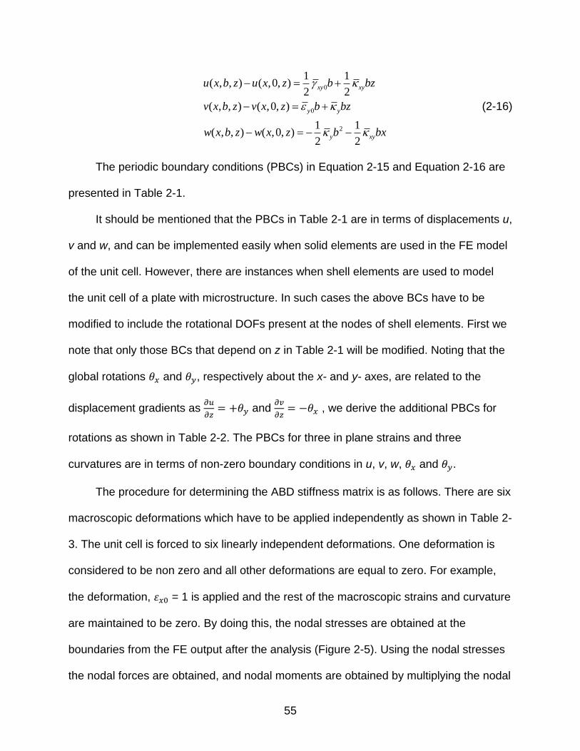
55
0
0
2
1 1( , , ) ( ,0, )
2 2
( , , ) ( ,0, )
1 1( , , ) ( ,0, )
2 2
xy xy
y y
y xy
u x b z u x z b bz
v x b z v x z b bz
w x b z w x z b bx
(2-16)
The periodic boundary conditions (PBCs) in Equation 2-15 and Equation 2-16 are
presented in Table 2-1.
It should be mentioned that the PBCs in Table 2-1 are in terms of displacements u,
v and w, and can be implemented easily when solid elements are used in the FE model
of the unit cell. However, there are instances when shell elements are used to model
the unit cell of a plate with microstructure. In such cases the above BCs have to be
modified to include the rotational DOFs present at the nodes of shell elements. First we
note that only those BCs that depend on z in Table 2-1 will be modified. Noting that the
global rotations and , respectively about the x- and y- axes, are related to the
displacement gradients as
and
, we derive the additional PBCs for
rotations as shown in Table 2-2. The PBCs for three in plane strains and three
curvatures are in terms of non-zero boundary conditions in u, v, w, and .
The procedure for determining the ABD stiffness matrix is as follows. There are six
macroscopic deformations which have to be applied independently as shown in Table 2-
3. The unit cell is forced to six linearly independent deformations. One deformation is
considered to be non zero and all other deformations are equal to zero. For example,
the deformation, = 1 is applied and the rest of the macroscopic strains and curvature
are maintained to be zero. By doing this, the nodal stresses are obtained at the
boundaries from the FE output after the analysis (Figure 2-5). Using the nodal stresses
the nodal forces are obtained, and nodal moments are obtained by multiplying the nodal
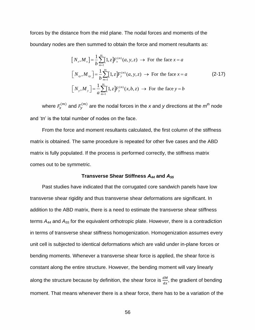
56
forces by the distance from the mid plane. The nodal forces and moments of the
boundary nodes are then summed to obtain the force and moment resultants as:
( )
1
( )
1
( )
1
1, 1, ( , , ) For the face
1, 1, ( , , ) For the face
1, 1, ( , , ) For the face
tnm
x x x
m
tnm
xy xy y
m
tnm
y y y
m
N M z F a y z x ab
N M z F a y z x ab
N M z F x b z y ba
(2-17)
where
and
are the nodal forces in the x and y directions at the mth node
and „tn‟ is the total number of nodes on the face.
From the force and moment resultants calculated, the first column of the stiffness
matrix is obtained. The same procedure is repeated for other five cases and the ABD
matrix is fully populated. If the process is performed correctly, the stiffness matrix
comes out to be symmetric.
Transverse Shear Stiffness A44 and A55
Past studies have indicated that the corrugated core sandwich panels have low
transverse shear rigidity and thus transverse shear deformations are significant. In
addition to the ABD matrix, there is a need to estimate the transverse shear stiffness
terms A44 and A55 for the equivalent orthotropic plate. However, there is a contradiction
in terms of transverse shear stiffness homogenization. Homogenization assumes every
unit cell is subjected to identical deformations which are valid under in-plane forces or
bending moments. Whenever a transverse shear force is applied, the shear force is
constant along the entire structure. However, the bending moment will vary linearly
along the structure because by definition, the shear force is
, the gradient of bending
moment. That means whenever there is a shear force, there has to be a variation of the
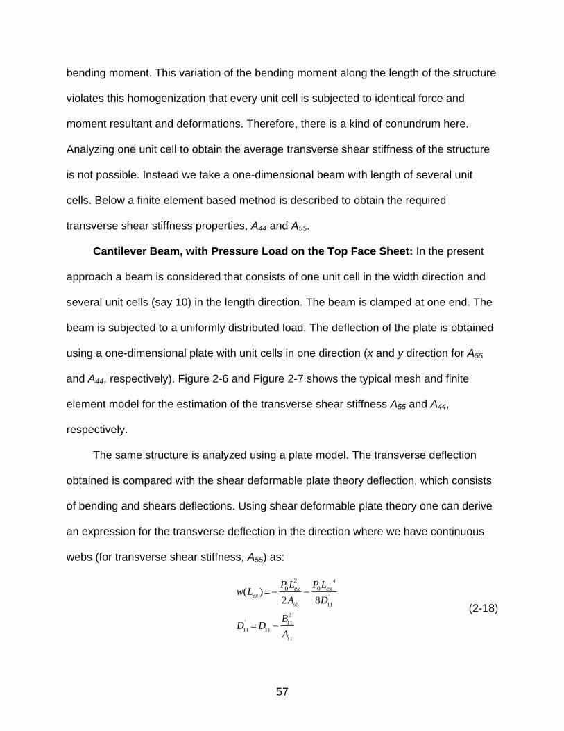
57
bending moment. This variation of the bending moment along the length of the structure
violates this homogenization that every unit cell is subjected to identical force and
moment resultant and deformations. Therefore, there is a kind of conundrum here.
Analyzing one unit cell to obtain the average transverse shear stiffness of the structure
is not possible. Instead we take a one-dimensional beam with length of several unit
cells. Below a finite element based method is described to obtain the required
transverse shear stiffness properties, A44 and A55.
Cantilever Beam, with Pressure Load on the Top Face Sheet: In the present
approach a beam is considered that consists of one unit cell in the width direction and
several unit cells (say 10) in the length direction. The beam is clamped at one end. The
beam is subjected to a uniformly distributed load. The deflection of the plate is obtained
using a one-dimensional plate with unit cells in one direction (x and y direction for A55
and A44, respectively). Figure 2-6 and Figure 2-7 shows the typical mesh and finite
element model for the estimation of the transverse shear stiffness A55 and A44,
respectively.
The same structure is analyzed using a plate model. The transverse deflection
obtained is compared with the shear deformable plate theory deflection, which consists
of bending and shears deflections. Using shear deformable plate theory one can derive
an expression for the transverse deflection in the direction where we have continuous
webs (for transverse shear stiffness, A55) as:
4
'
55 11
2
' 11
11 11
11
2
0 0( )2 8
ex exex
P L P Lw L
A D
BD D
A
(2-18)
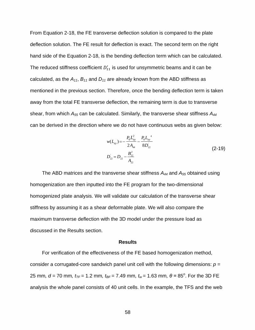
58
From Equation 2-18, the FE transverse deflection solution is compared to the plate
deflection solution. The FE result for deflection is exact. The second term on the right
hand side of the Equation 2-18, is the bending deflection term which can be calculated.
The reduced stiffness coefficient is used for unsymmetric beams and it can be
calculated, as the A11, B11 and D11 are already known from the ABD stiffness as
mentioned in the previous section. Therefore, once the bending deflection term is taken
away from the total FE transverse deflection, the remaining term is due to transverse
shear, from which A55 can be calculated. Similarly, the transverse shear stiffness A44
can be derived in the direction where we do not have continuous webs as given below:
4
'
44 22
2
' 22
22 22
22
2
0 0( )
2 8
ey ey
ey
P P Lw L
A D
BD D
A
L
(2-19)
The ABD matrices and the transverse shear stiffness A44 and A55 obtained using
homogenization are then inputted into the FE program for the two-dimensional
homogenized plate analysis. We will validate our calculation of the transverse shear
stiffness by assuming it as a shear deformable plate. We will also compare the
maximum transverse deflection with the 3D model under the pressure load as
discussed in the Results section.
Results
For verification of the effectiveness of the FE based homogenization method,
consider a corrugated-core sandwich panel unit cell with the following dimensions: p =
25 mm, d = 70 mm, tTF = 1.2 mm, tBF = 7.49 mm, tw = 1.63 mm, θ = 85o. For the 3D FE
analysis the whole panel consists of 40 unit cells. In the example, the TFS and the web
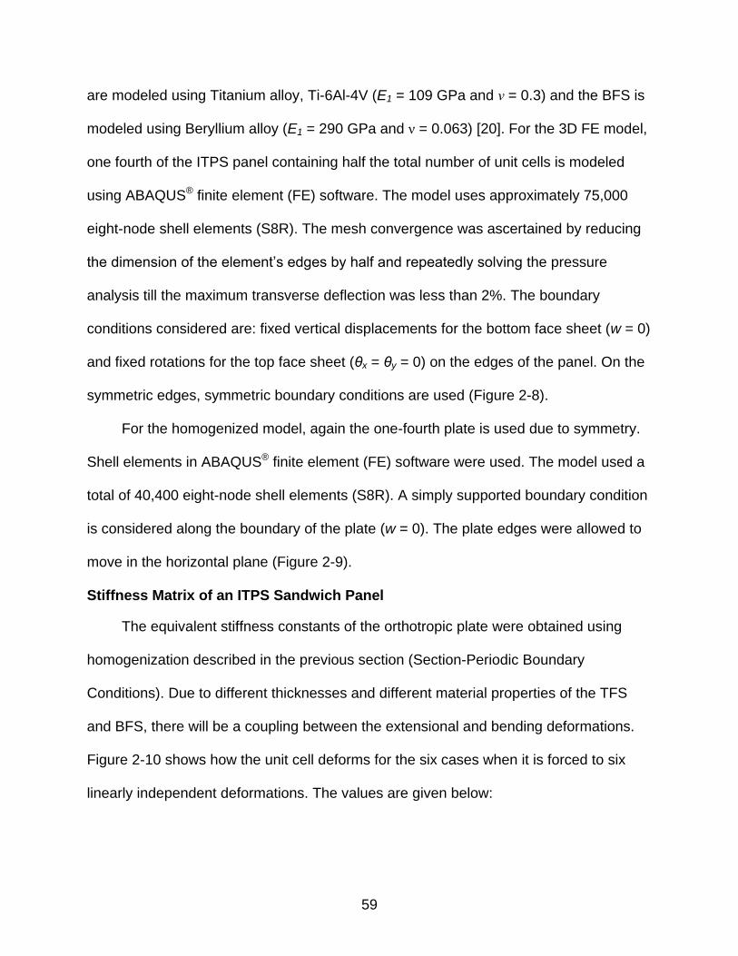
59
are modeled using Titanium alloy, Ti-6Al-4V (E1 = 109 GPa and ν = 0.3) and the BFS is
modeled using Beryllium alloy (E1 = 290 GPa and ν = 0.063) [20]. For the 3D FE model,
one fourth of the ITPS panel containing half the total number of unit cells is modeled
using ABAQUS® finite element (FE) software. The model uses approximately 75,000
eight-node shell elements (S8R). The mesh convergence was ascertained by reducing
the dimension of the element‟s edges by half and repeatedly solving the pressure
analysis till the maximum transverse deflection was less than 2%. The boundary
conditions considered are: fixed vertical displacements for the bottom face sheet (w = 0)
and fixed rotations for the top face sheet (θx = θy = 0) on the edges of the panel. On the
symmetric edges, symmetric boundary conditions are used (Figure 2-8).
For the homogenized model, again the one-fourth plate is used due to symmetry.
Shell elements in ABAQUS® finite element (FE) software were used. The model used a
total of 40,400 eight-node shell elements (S8R). A simply supported boundary condition
is considered along the boundary of the plate (w = 0). The plate edges were allowed to
move in the horizontal plane (Figure 2-9).
Stiffness Matrix of an ITPS Sandwich Panel
The equivalent stiffness constants of the orthotropic plate were obtained using
homogenization described in the previous section (Section-Periodic Boundary
Conditions). Due to different thicknesses and different material properties of the TFS
and BFS, there will be a coupling between the extensional and bending deformations.
Figure 2-10 shows how the unit cell deforms for the six cases when it is forced to six
linearly independent deformations. The values are given below:
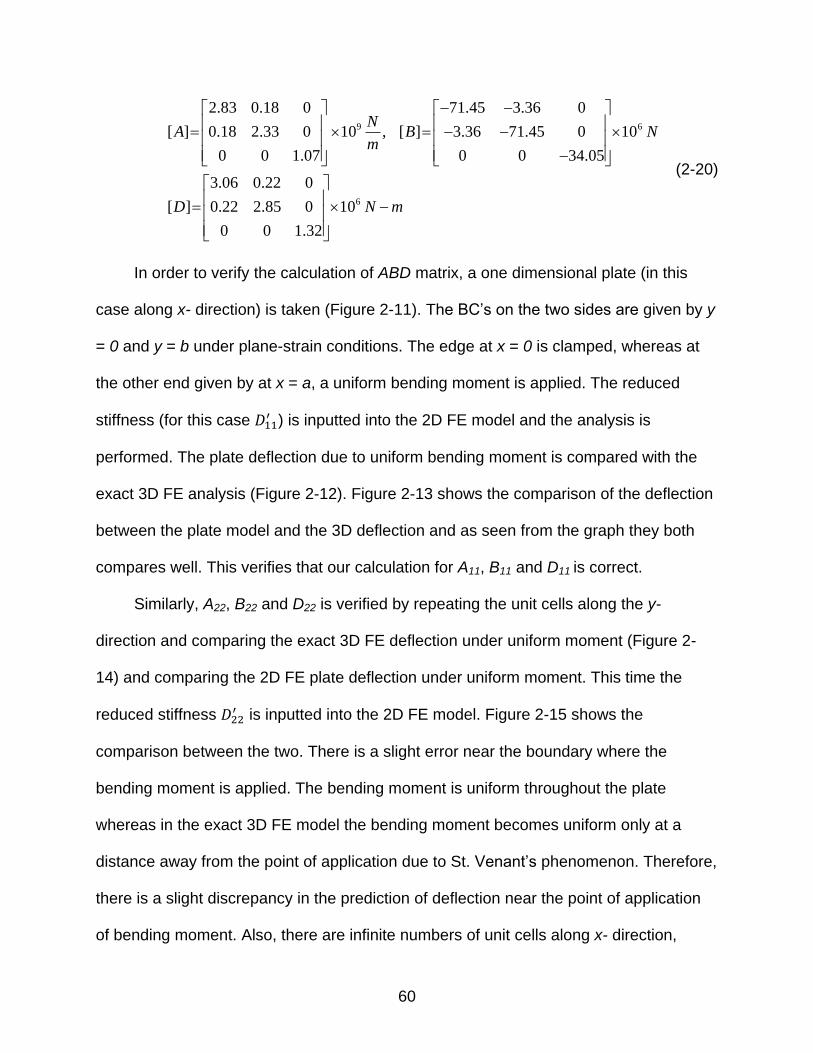
60
9 6
6
2.83 0.18 0 71.45 3.36 0
[ ] 0.18 2.33 0 10 , [ ] 3.36 71.45 0 10
0 0 1.07 0 0 34.05
3.06 0.22 0
[ ] 0.22 2.85 0 10
0 0 1.32
NA B N
m
D N m
(2-20)
In order to verify the calculation of ABD matrix, a one dimensional plate (in this
case along x- direction) is taken (Figure 2-11). The BC‟s on the two sides are given by y
= 0 and y = b under plane-strain conditions. The edge at x = 0 is clamped, whereas at
the other end given by at x = a, a uniform bending moment is applied. The reduced
stiffness (for this case ) is inputted into the 2D FE model and the analysis is
performed. The plate deflection due to uniform bending moment is compared with the
exact 3D FE analysis (Figure 2-12). Figure 2-13 shows the comparison of the deflection
between the plate model and the 3D deflection and as seen from the graph they both
compares well. This verifies that our calculation for A11, B11 and D11 is correct.
Similarly, A22, B22 and D22 is verified by repeating the unit cells along the y-
direction and comparing the exact 3D FE deflection under uniform moment (Figure 2-
14) and comparing the 2D FE plate deflection under uniform moment. This time the
reduced stiffness is inputted into the 2D FE model. Figure 2-15 shows the
comparison between the two. There is a slight error near the boundary where the
bending moment is applied. The bending moment is uniform throughout the plate
whereas in the exact 3D FE model the bending moment becomes uniform only at a
distance away from the point of application due to St. Venant‟s phenomenon. Therefore,
there is a slight discrepancy in the prediction of deflection near the point of application
of bending moment. Also, there are infinite numbers of unit cells along x- direction,
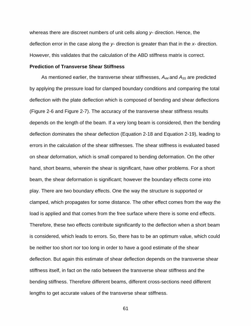
61
whereas there are discreet numbers of unit cells along y- direction. Hence, the
deflection error in the case along the y- direction is greater than that in the x- direction.
However, this validates that the calculation of the ABD stiffness matrix is correct.
Prediction of Transverse Shear Stiffness
As mentioned earlier, the transverse shear stiffnesses, A44 and A55 are predicted
by applying the pressure load for clamped boundary conditions and comparing the total
deflection with the plate deflection which is composed of bending and shear deflections
(Figure 2-6 and Figure 2-7). The accuracy of the transverse shear stiffness results
depends on the length of the beam. If a very long beam is considered, then the bending
deflection dominates the shear deflection (Equation 2-18 and Equation 2-19), leading to
errors in the calculation of the shear stiffnesses. The shear stiffness is evaluated based
on shear deformation, which is small compared to bending deformation. On the other
hand, short beams, wherein the shear is significant, have other problems. For a short
beam, the shear deformation is significant; however the boundary effects come into
play. There are two boundary effects. One the way the structure is supported or
clamped, which propagates for some distance. The other effect comes from the way the
load is applied and that comes from the free surface where there is some end effects.
Therefore, these two effects contribute significantly to the deflection when a short beam
is considered, which leads to errors. So, there has to be an optimum value, which could
be neither too short nor too long in order to have a good estimate of the shear
deflection. But again this estimate of shear deflection depends on the transverse shear
stiffness itself, in fact on the ratio between the transverse shear stiffness and the
bending stiffness. Therefore different beams, different cross-sections need different
lengths to get accurate values of the transverse shear stiffness.
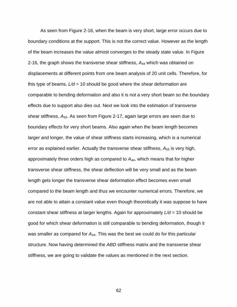
62
As seen from Figure 2-16, when the beam is very short, large error occurs due to
boundary conditions at the support. This is not the correct value. However as the length
of the beam increases the value almost converges to the steady state value. In Figure
2-16, the graph shows the transverse shear stiffness, A44 which was obtained on
displacements at different points from one beam analysis of 20 unit cells. Therefore, for
this type of beams, L/d = 10 should be good where the shear deformation are
comparable to bending deformation and also it is not a very short beam so the boundary
effects due to support also dies out. Next we look into the estimation of transverse
shear stiffness, A55. As seen from Figure 2-17, again large errors are seen due to
boundary effects for very short beams. Also again when the beam length becomes
larger and longer, the value of shear stiffness starts increasing, which is a numerical
error as explained earlier. Actually the transverse shear stiffness, A55 is very high,
approximately three orders high as compared to A44, which means that for higher
transverse shear stiffness, the shear deflection will be very small and as the beam
length gets longer the transverse shear deformation effect becomes even small
compared to the beam length and thus we encounter numerical errors. Therefore, we
are not able to attain a constant value even though theoretically it was suppose to have
constant shear stiffness at larger lengths. Again for approximately L/d = 10 should be
good for which shear deformation is still comparable to bending deformation, though it
was smaller as compared for A44. This was the best we could do for this particular
structure. Now having determined the ABD stiffness matrix and the transverse shear
stiffness, we are going to validate the values as mentioned in the next section.
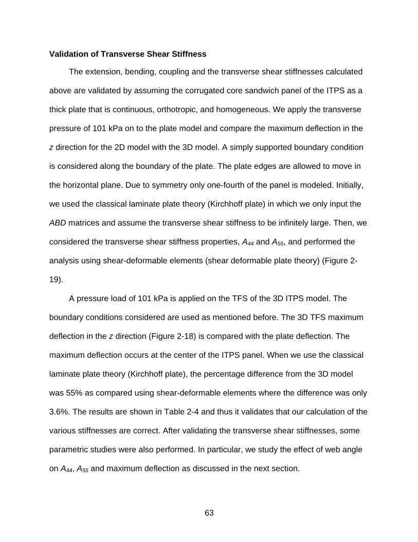
63
Validation of Transverse Shear Stiffness
The extension, bending, coupling and the transverse shear stiffnesses calculated
above are validated by assuming the corrugated core sandwich panel of the ITPS as a
thick plate that is continuous, orthotropic, and homogeneous. We apply the transverse
pressure of 101 kPa on to the plate model and compare the maximum deflection in the
z direction for the 2D model with the 3D model. A simply supported boundary condition
is considered along the boundary of the plate. The plate edges are allowed to move in
the horizontal plane. Due to symmetry only one-fourth of the panel is modeled. Initially,
we used the classical laminate plate theory (Kirchhoff plate) in which we only input the
ABD matrices and assume the transverse shear stiffness to be infinitely large. Then, we
considered the transverse shear stiffness properties, A44 and A55, and performed the
analysis using shear-deformable elements (shear deformable plate theory) (Figure 2-
19).
A pressure load of 101 kPa is applied on the TFS of the 3D ITPS model. The
boundary conditions considered are used as mentioned before. The 3D TFS maximum
deflection in the z direction (Figure 2-18) is compared with the plate deflection. The
maximum deflection occurs at the center of the ITPS panel. When we use the classical
laminate plate theory (Kirchhoff plate), the percentage difference from the 3D model
was 55% as compared using shear-deformable elements where the difference was only
3.6%. The results are shown in Table 2-4 and thus it validates that our calculation of the
various stiffnesses are correct. After validating the transverse shear stiffnesses, some
parametric studies were also performed. In particular, we study the effect of web angle
on A44, A55 and maximum deflection as discussed in the next section.
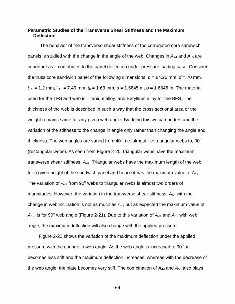
64
Parametric Studies of the Transverse Shear Stiffness and the Maximum Deflection
The behavior of the transverse shear stiffness of the corrugated core sandwich
panels is studied with the change in the angle of the web. Changes in A44 and A55 are
important as it contributes to the panel deflection under pressure loading case. Consider
the truss core sandwich panel of the following dimensions: p = 84.25 mm, d = 70 mm,
tTF = 1.2 mm, tBF = 7.49 mm, tw = 1.63 mm, a = 1.6845 m, b = 1.6845 m. The material
used for the TFS and web is Titanium alloy, and Beryllium alloy for the BFS. The
thickness of the web is described in such a way that the cross sectional area or the
weight remains same for any given web angle. By doing this we can understand the
variation of the stiffness to the change in angle only rather than changing the angle and
thickness. The web angles are varied from 40o, i.e. almost like triangular webs to, 90o
(rectangular webs). As seen from Figure 2-20, triangular webs have the maximum
transverse shear stiffness, A44. Triangular webs have the maximum length of the web
for a given height of the sandwich panel and hence it has the maximum value of A44.
The variation of A44 from 90o webs to triangular webs is almost two orders of
magnitudes. However, the variation in the transverse shear stiffness, A55 with the
change in web inclination is not as much as A44 but as expected the maximum value of
A55, is for 90o web angle (Figure 2-21). Due to this variation of A44 and A55 with web
angle, the maximum deflection will also change with the applied pressure.
Figure 2-22 shows the variation of the maximum deflection under the applied
pressure with the change in web angle. As the web angle is increased to 90o, it
becomes less stiff and the maximum deflection increases, whereas with the decrease of
the web angle, the plate becomes very stiff. The combination of A44 and A55 also plays
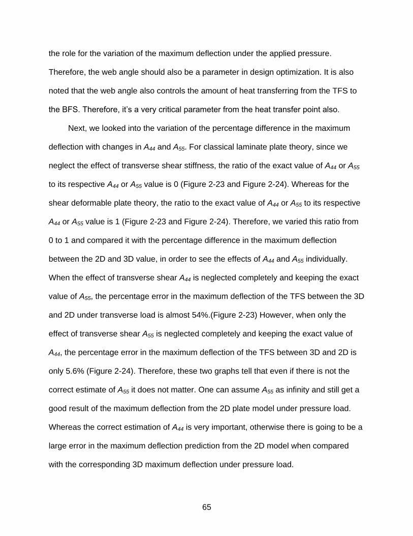
65
the role for the variation of the maximum deflection under the applied pressure.
Therefore, the web angle should also be a parameter in design optimization. It is also
noted that the web angle also controls the amount of heat transferring from the TFS to
the BFS. Therefore, it‟s a very critical parameter from the heat transfer point also.
Next, we looked into the variation of the percentage difference in the maximum
deflection with changes in A44 and A55. For classical laminate plate theory, since we
neglect the effect of transverse shear stiffness, the ratio of the exact value of A44 or A55
to its respective A44 or A55 value is 0 (Figure 2-23 and Figure 2-24). Whereas for the
shear deformable plate theory, the ratio to the exact value of A44 or A55 to its respective
A44 or A55 value is 1 (Figure 2-23 and Figure 2-24). Therefore, we varied this ratio from
0 to 1 and compared it with the percentage difference in the maximum deflection
between the 2D and 3D value, in order to see the effects of A44 and A55 individually.
When the effect of transverse shear A44 is neglected completely and keeping the exact
value of A55, the percentage error in the maximum deflection of the TFS between the 3D
and 2D under transverse load is almost 54%.(Figure 2-23) However, when only the
effect of transverse shear A55 is neglected completely and keeping the exact value of
A44, the percentage error in the maximum deflection of the TFS between 3D and 2D is
only 5.6% (Figure 2-24). Therefore, these two graphs tell that even if there is not the
correct estimate of A55 it does not matter. One can assume A55 as infinity and still get a
good result of the maximum deflection from the 2D plate model under pressure load.
Whereas the correct estimation of A44 is very important, otherwise there is going to be a
large error in the maximum deflection prediction from the 2D model when compared
with the corresponding 3D maximum deflection under pressure load.
66
Concluding Remarks
In this chapter, a finite element based homogenization procedure is developed for
modeling corrugate sandwich panels as a 2D orthotropic plate. Corrugated sandwich
panels are potential candidates for the integrated thermal protection systems for future
aerospace vehicles. The periodic boundary conditions are derived in a formal way to
obtain the bending, extensional, and coupling stiffness for an ITPS panel using finite
element approach. The transverse shear stiffness properties are also derived using an
FE approach. The biggest advantage of finite element based micromechanical analysis
is that it is capable of handling any combination of material properties for face sheets
and webs, and any geometry.
Effect of web angle on various stiffness properties of the ITPS was studied. For a
given plate dimension and loading, maximum deflection occurs for web angle of 90-
degrees whereas the minimum deflection occurred when the webs take a triangular
configuration. Finally the results of various stiffnesses are validated by applying a
transverse pressure on to the 2D plate model and 3D ITPS panel. Agreement between
2D and 3D results for transverse deflection was good.
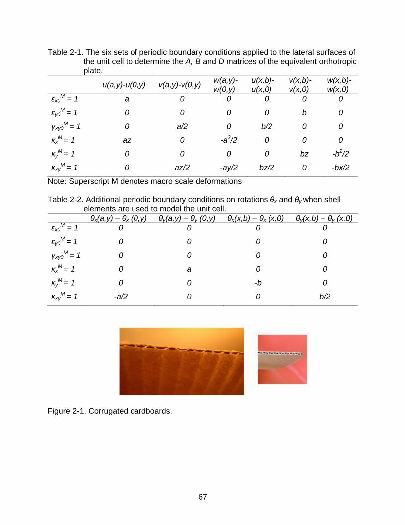
67
Table 2-1. The six sets of periodic boundary conditions applied to the lateral surfaces of the unit cell to determine the A, B and D matrices of the equivalent orthotropic plate.
u(a,y)-u(0,y) v(a,y)-v(0,y) w(a,y)-w(0,y)
u(x,b)-u(x,0)
v(x,b)-v(x,0)
w(x,b)-w(x,0)
εx0M = 1 a 0 0 0 0 0
εy0M = 1 0 0 0 0 b 0
γxy0M = 1 0 a/2 0 b/2 0 0
κxM
= 1 az 0 -a2/2 0 0 0
κyM
= 1 0 0 0 0 bz -b2/2
κxyM
= 1 0 az/2 -ay/2 bz/2 0 -bx/2
Note: Superscript M denotes macro scale deformations
Table 2-2. Additional periodic boundary conditions on rotations θx and θy when shell elements are used to model the unit cell.
θx(a,y) – θx (0,y) θy(a,y) – θy (0,y) θx(x,b) – θx (x,0) θy(x,b) – θy (x,0)
εx0M = 1 0 0 0 0
εy0M = 1 0 0 0 0
γxy0M = 1 0 0 0 0
κxM
= 1 0 a 0 0
κyM
= 1 0 0 -b 0
κxyM
= 1 -a/2 0 0 b/2
Figure 2-1. Corrugated cardboards.
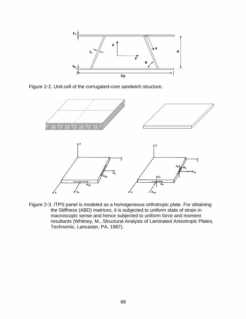
68
Figure 2-2. Unit-cell of the corrugated-core sandwich structure.
Figure 2-3. ITPS panel is modeled as a homogeneous orthotropic plate. For obtaining the Stiffness (ABD) matrices, it is subjected to uniform state of strain in macroscopic sense and hence subjected to uniform force and moment resultants (Whitney, M., Structural Analysis of Laminated Anisotropic Plates, Technomic, Lancaster, PA, 1987).
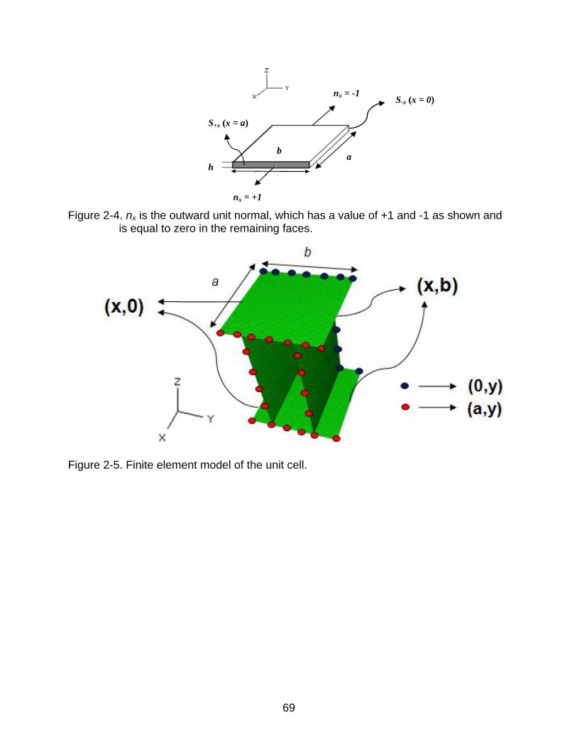
69
Figure 2-4. nx is the outward unit normal, which has a value of +1 and -1 as shown and is equal to zero in the remaining faces.
Figure 2-5. Finite element model of the unit cell.
S+x (x = a)
S-x (x = 0)
nx = +1
a b
h
nx = -1
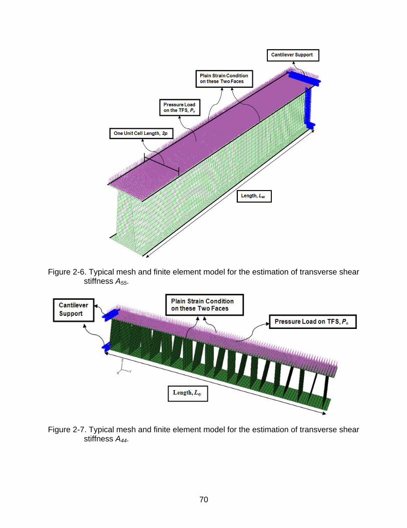
70
Figure 2-6. Typical mesh and finite element model for the estimation of transverse shear stiffness A55.
Figure 2-7. Typical mesh and finite element model for the estimation of transverse shear stiffness A44.
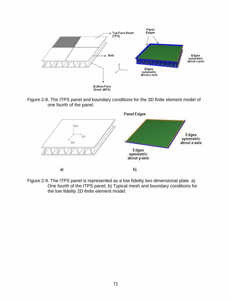
71
Figure 2-8. The ITPS panel and boundary conditions for the 3D finite element model of one fourth of the panel.
Figure 2-9. The ITPS panel is represented as a low fidelity two dimensional plate. a) One fourth of the ITPS panel, b) Typical mesh and boundary conditions for the low fidelity 2D finite element model.
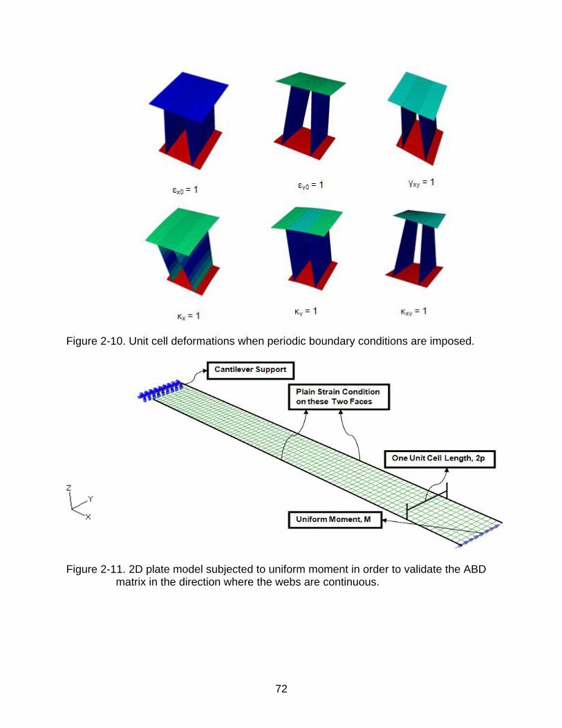
72
Figure 2-10. Unit cell deformations when periodic boundary conditions are imposed.
Figure 2-11. 2D plate model subjected to uniform moment in order to validate the ABD matrix in the direction where the webs are continuous.
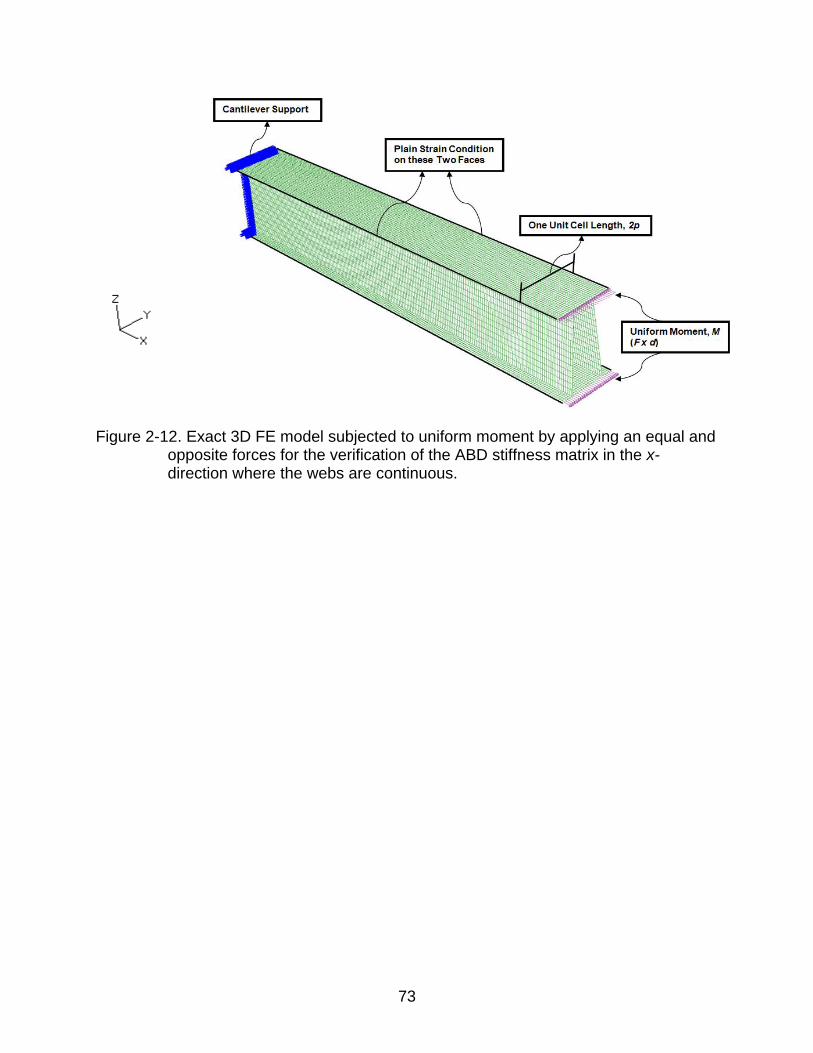
73
Figure 2-12. Exact 3D FE model subjected to uniform moment by applying an equal and opposite forces for the verification of the ABD stiffness matrix in the x- direction where the webs are continuous.
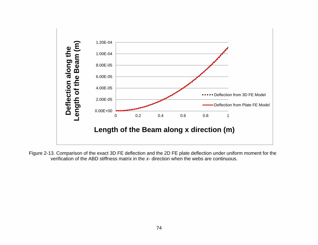
74
Figure 2-13. Comparison of the exact 3D FE deflection and the 2D FE plate deflection under uniform moment for the verification of the ABD stiffness matrix in the x- direction when the webs are continuous.
0.00E+00
2.00E-05
4.00E-05
6.00E-05
8.00E-05
1.00E-04
1.20E-04
0 0.2 0.4 0.6 0.8 1De
fle
cti
on
alo
ng
th
e
Len
gth
of
the B
eam
(m
)
Length of the Beam along x direction (m)
Deflection from 3D FE Model
Deflection from Plate FE Model
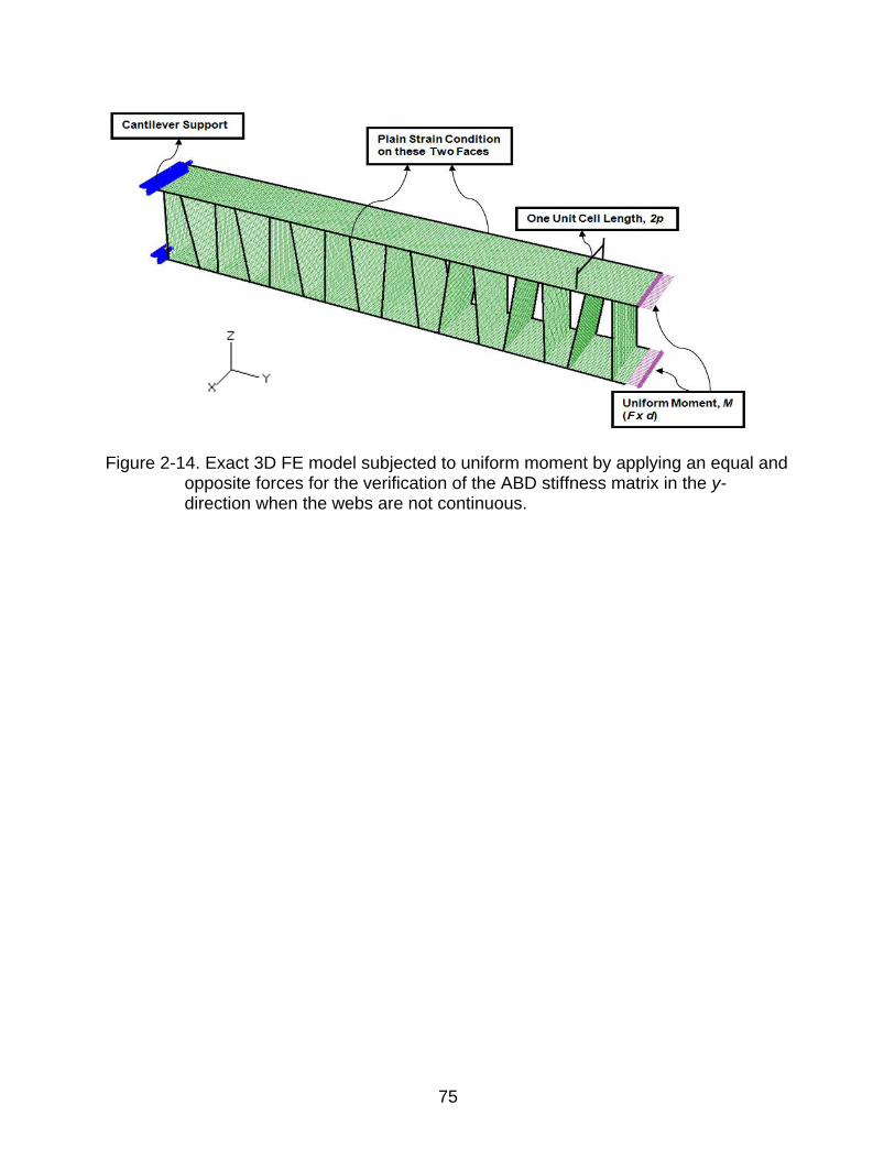
75
Figure 2-14. Exact 3D FE model subjected to uniform moment by applying an equal and opposite forces for the verification of the ABD stiffness matrix in the y- direction when the webs are not continuous.
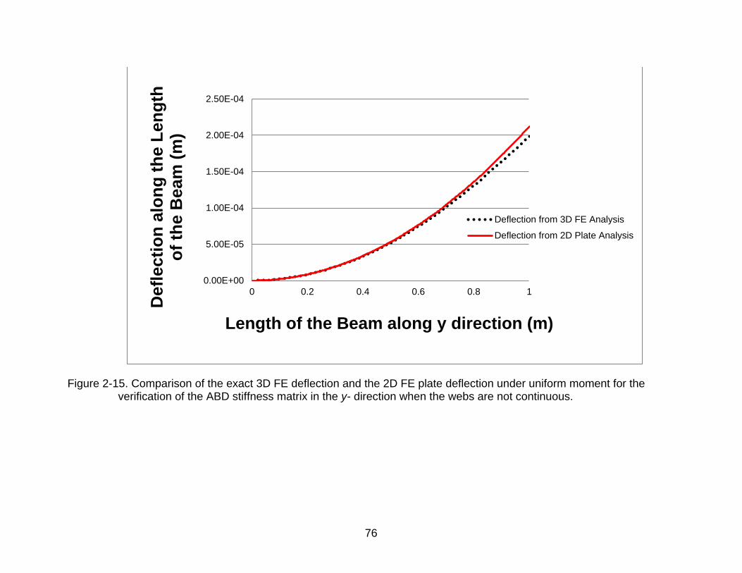
76
Figure 2-15. Comparison of the exact 3D FE deflection and the 2D FE plate deflection under uniform moment for the verification of the ABD stiffness matrix in the y- direction when the webs are not continuous.
0.00E+00
5.00E-05
1.00E-04
1.50E-04
2.00E-04
2.50E-04
0 0.2 0.4 0.6 0.8 1
Defl
ecti
on
alo
ng
th
e L
en
gth
o
f th
e B
eam
(m
)
Length of the Beam along y direction (m)
Deflection from 3D FE Analysis
Deflection from 2D Plate Analysis
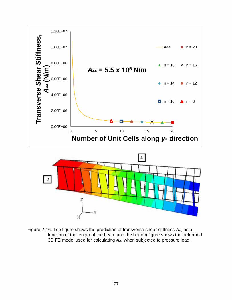
77
Figure 2-16. Top figure shows the prediction of transverse shear stiffness A44 as a function of the length of the beam and the bottom figure shows the deformed 3D FE model used for calculating A44 when subjected to pressure load.
0.00E+00
2.00E+06
4.00E+06
6.00E+06
8.00E+06
1.00E+07
1.20E+07
0 5 10 15 20
Tra
nsvers
e S
hear
Sti
ffn
ess,
A4
4 (
N/m
)
Number of Unit Cells along y- direction
A44 n = 20
n = 18 n = 16
n = 14 n = 12
n = 10 n = 8
A44 = 5.5 x 10⁵ N/m
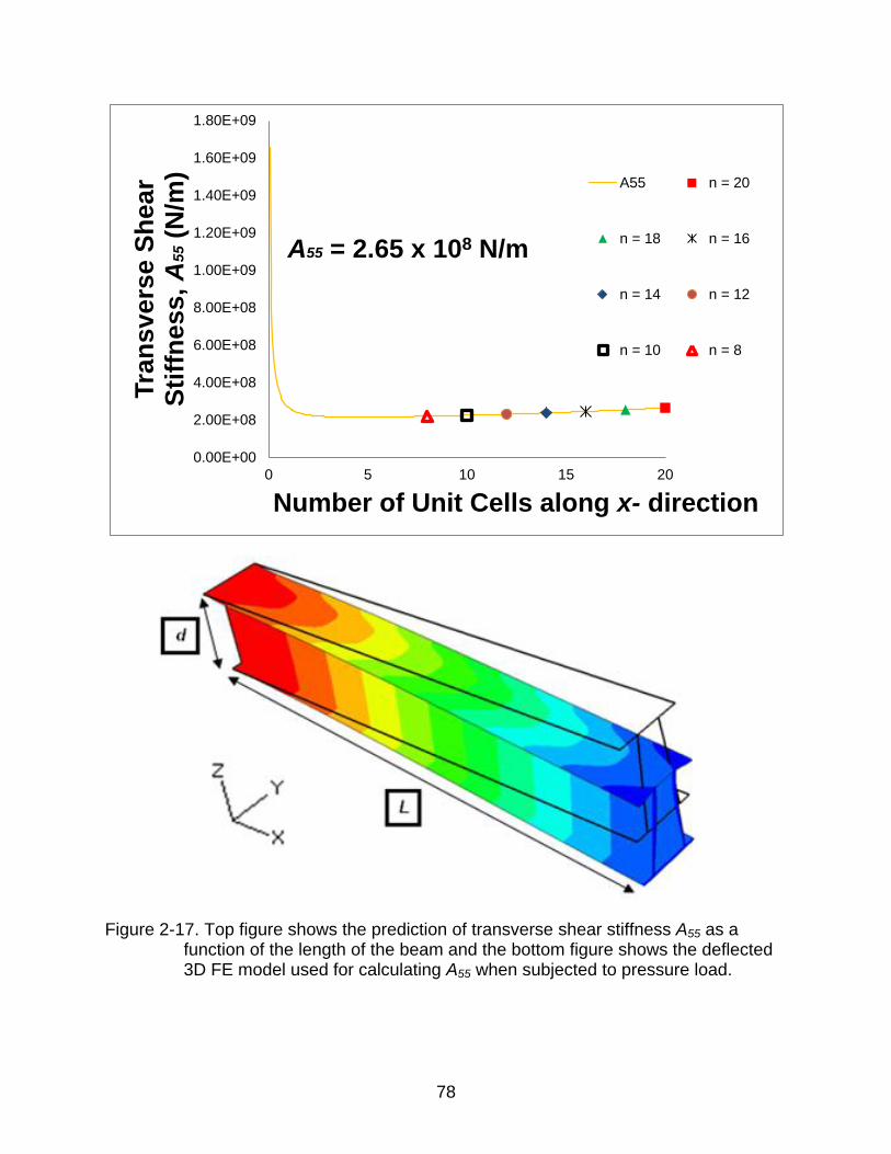
78
Figure 2-17. Top figure shows the prediction of transverse shear stiffness A55 as a function of the length of the beam and the bottom figure shows the deflected 3D FE model used for calculating A55 when subjected to pressure load.
0.00E+00
2.00E+08
4.00E+08
6.00E+08
8.00E+08
1.00E+09
1.20E+09
1.40E+09
1.60E+09
1.80E+09
0 5 10 15 20
Tra
nsvers
e S
hear
Sti
ffn
ess,
A5
5 (
N/m
)
Number of Unit Cells along x- direction
A55 n = 20
n = 18 n = 16
n = 14 n = 12
n = 10 n = 8
A55 = 2.65 x 10⁸ N/m
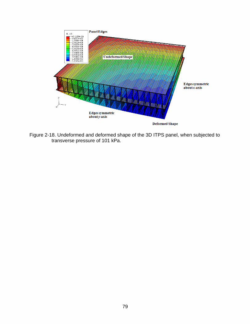
79
Figure 2-18. Undeformed and deformed shape of the 3D ITPS panel, when subjected to transverse pressure of 101 kPa.
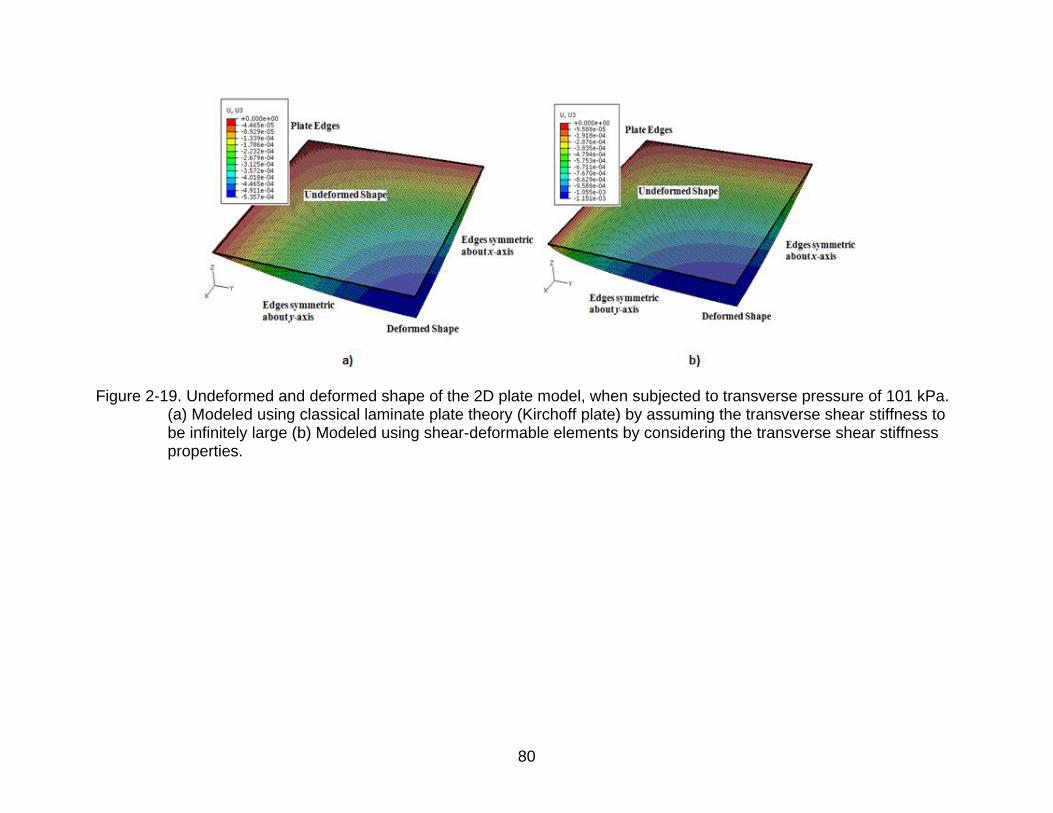
80
Figure 2-19. Undeformed and deformed shape of the 2D plate model, when subjected to transverse pressure of 101 kPa. (a) Modeled using classical laminate plate theory (Kirchoff plate) by assuming the transverse shear stiffness to be infinitely large (b) Modeled using shear-deformable elements by considering the transverse shear stiffness properties.
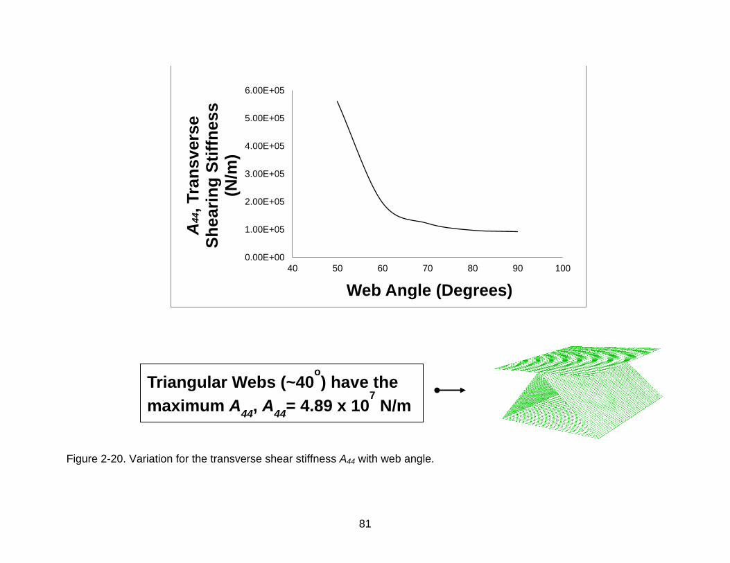
81
Figure 2-20. Variation for the transverse shear stiffness A44 with web angle.
0.00E+00
1.00E+05
2.00E+05
3.00E+05
4.00E+05
5.00E+05
6.00E+05
40 50 60 70 80 90 100
A4
4, Tra
nsvers
e
Sh
eari
ng
Sti
ffn
ess
(N/m
)
Web Angle (Degrees)
Triangular Webs (~40o) have the
maximum A44
, A44
= 4.89 x 10⁷ N/m
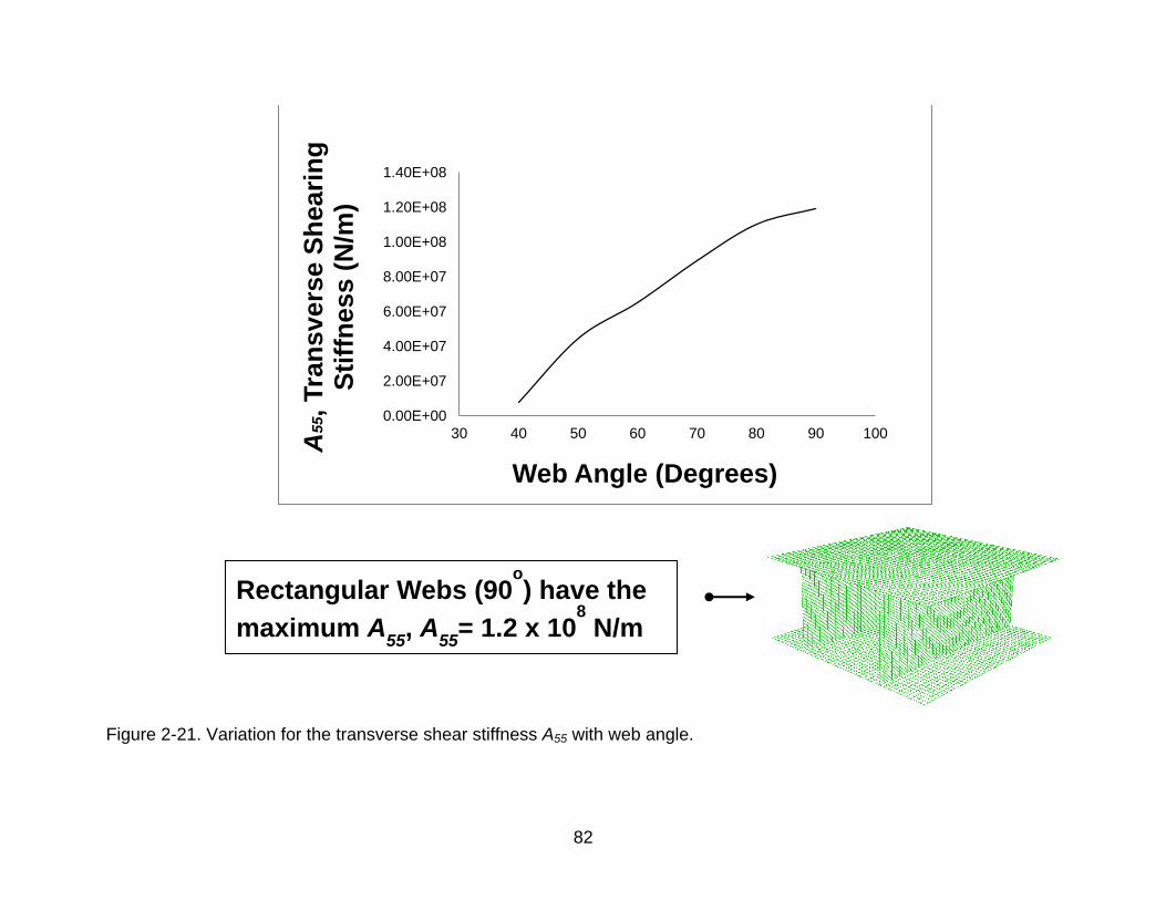
82
Figure 2-21. Variation for the transverse shear stiffness A55 with web angle.
0.00E+00
2.00E+07
4.00E+07
6.00E+07
8.00E+07
1.00E+08
1.20E+08
1.40E+08
30 40 50 60 70 80 90 100
A5
5, Tra
nsvers
e S
heari
ng
S
tiff
ness (
N/m
)
Web Angle (Degrees)
Rectangular Webs (90o) have the
maximum A55
, A55
= 1.2 x 10⁸ N/m
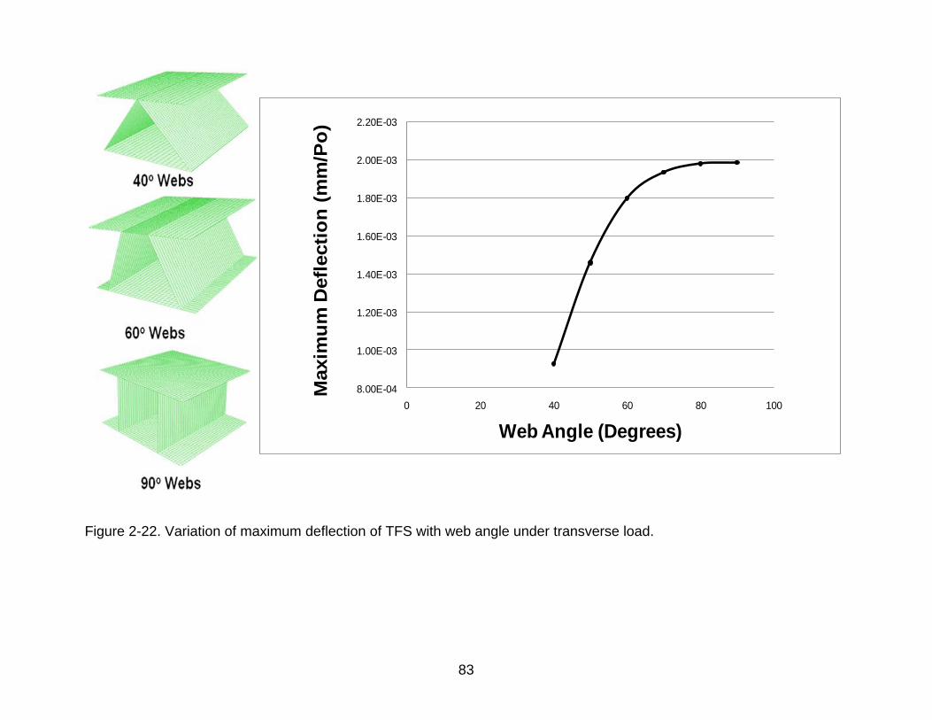
83
8.00E-04
1.00E-03
1.20E-03
1.40E-03
1.60E-03
1.80E-03
2.00E-03
2.20E-03
0 20 40 60 80 100
Maxim
um
Defl
ecti
on
(m
m/P
o)
Web Angle (Degrees)
Figure 2-22. Variation of maximum deflection of TFS with web angle under transverse load.
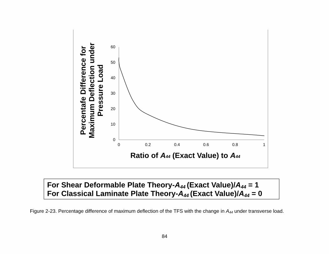
84
Figure 2-23. Percentage difference of maximum deflection of the TFS with the change in A44 under transverse load.
0
10
20
30
40
50
60
0 0.2 0.4 0.6 0.8 1
Perc
en
tafe
Dif
fere
nce f
or
Maxim
um
Defl
ecti
on
un
der
Pre
ss
ure
Lo
ad
Ratio of A44 (Exact Value) to A44
For Shear Deformable Plate Theory-A44 (Exact Value)/A44 = 1 For Classical Laminate Plate Theory-A44 (Exact Value)/A44 = 0
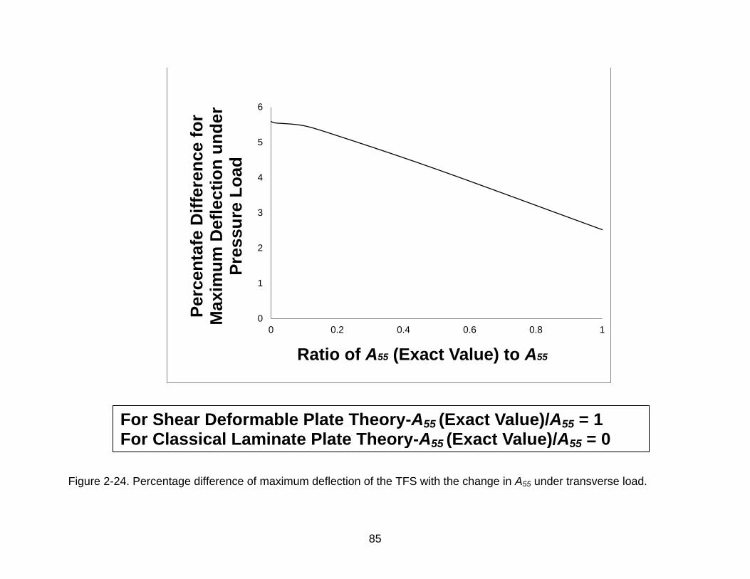
85
Figure 2-24. Percentage difference of maximum deflection of the TFS with the change in A55 under transverse load.
0
1
2
3
4
5
6
0 0.2 0.4 0.6 0.8 1
Perc
en
tafe
Dif
fere
nce f
or
Maxim
um
Defl
ecti
on
un
der
Pre
ss
ure
Lo
ad
Ratio of A55 (Exact Value) to A55
For Shear Deformable Plate Theory-A55 (Exact Value)/A55 = 1 For Classical Laminate Plate Theory-A55 (Exact Value)/A55 = 0
86
CHAPTER 3 STRESS AND BUCKLING ANALYSIS UNDER PRESSURE AND THERMAL LOADS
ON AN INTEGRATED THERMAL PROTECTION SYSTEM PANEL
The ITPS is the outermost covering of the space vehicle. It is exposed to different
types of environments during different phases of flight like ground debris strike, lightning
strike, bird strike, rain/rain erosion, and on-orbit debris/micrometeoroid hypervelocity
impact [10]. The ITPS should be able to withstand the aerodynamic heating loads to
maintain the structure of the space vehicle within an acceptable temperature range. The
hypersonic vehicle enters with a very high angle (40 degrees) of attack. It should be
able to provide an acceptable aerodynamic surface to prevent premature transition to
turbulence due to this surface heating and maintain acceptable performance. It is also
exposed to pressure load from the transverse aerodynamic pressure or pressurized
crew compartment, which tend to push the ITPS panel off the vehicle or into the vehicle,
bending the outer surface and loading attachments and support hardware [9]. These
pressures vary with time and location on the vehicle.
If three dimensional finite element methods were used to determine the response
of a sandwich structure, the number of nodes and elements needed to properly model
the structure can be excessive; as a result a full 3-D finite element analysis is not
economical to conduct a preliminary analysis. Such panels may also be represented as
a plate that is continuous, orthotropic, and homogenous, for which analytical [69]
solutions are available. The analytical model resulted in a reasonably good estimate of
stiffness properties - A, B and D matrices; however, the stresses in the web and face
sheets differed significantly as the homogenized plate could not faithfully represent the
local behavior of the ITPS. There was considerable difference between the analytical
2D and 3D models with widely varying geometries and material properties and hence it
87
was difficult to implement them in the design optimization environment. Hence, a finite
element method based homogenization and reverse homogenization procedure is
developed for calculating the deflections and stresses in the web and face sheets when
subjected to pressure and thermal loads.
The extensional stiffness matrix [A], coupling stiffness matrix [B], bending stiffness
[D], and the transverse shear stiffness terms A44 and A55 are calculated using finite
element by using periodic boundary condition as mentioned in Chapter 2. These
equivalent stiffness properties are then inputted to the plate finite element model for the
two-dimensional homogenized plate analysis under pressure and thermal loads. After
performing the plate analysis under pressure and thermal loading, the plate
deformations (strains and curvatures) were then reapplied applied to the unit-cell by the
process of reverse homogenization in order to obtain the detailed displacements and
stresses in the face sheets and the web of the ITPS. The results were then compared
with that from the 3D analysis of the ITPS. The entire homogenization and reverse
homogenization are shown in the flowchart in Figure 3-2. The FE based
homogenization and reverse was found to be more robust and could be performed with
any commercially available FE programs. The FE based homogenization and analysis
of the 2D plate is less expensive as compared to that of 3D.
As mentioned before, there are two important types of loads that need to be
considered in the design optimization of an ITPS. Both occur during the reentry phase
of the space vehicle. The two load cases are: (a) aerodynamic pressure acting on the
top face sheet; and (b) thermal stresses due to severe temperature gradient across the
thickness of the ITPS. These loads could cause the ITPS panel to fail by buckling,
88
and/or yielding. Knowing the panel behavior and failure modes when exposed to
different loading environments is important in the design because excessive deflection
of the panel leads to extremely high local aerodynamic heating or high stresses leads to
undesirable yielding and critical buckling. Therefore, the analysis of these two load
cases using the method of homogenization and reverse homogenization are described
in the following sections:
Uniform Pressure Loading Analysis
Aerodynamic pressure load during reentry for a space shuttle-like design is shown
in Figure 3-3. During reentry the pressure load on the outer surface of the vehicle is
considered to be zero. But after landing, the external pressure becomes equal to the
atmospheric pressure (Figure 3-3). TPS separates the crew compartment from the outer
shell. The crew compartment is under pressure apposite to human comfort. The space
between the crew compartment and the outer shell is assumed to be vented to the outer
atmosphere. Just prior to reentry, this vented space would be at zero pressure. During
reentry phase the pressure load on both sides of TPS is zero and hence there is no
pressure load applied on the ITPS panels during reentry phase. After the vehicle lands,
the outside pressure is equal to the atmospheric pressure. Even though the space
between crew compartment and the TPS is vented to the atmosphere, there will be a
certain lag time before the pressure on both sides of the TPS becomes equal. During
this lag time, there is a pressure load on the outer surface. We will consider the worst
case scenario, where the pressure load on the outer surface is considered equal to 1
atmosphere or 101,325 Pa. This pressure value is typical for the maximum pressure to
which the ITPS could be subjected to [67].
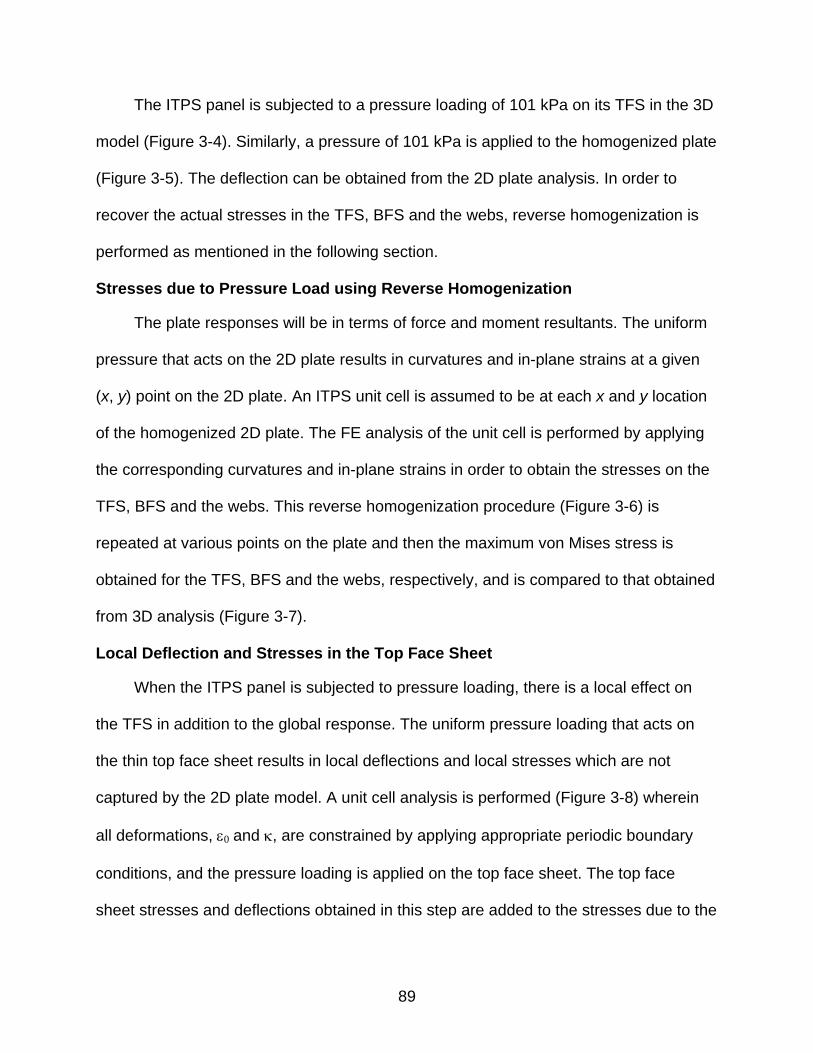
89
The ITPS panel is subjected to a pressure loading of 101 kPa on its TFS in the 3D
model (Figure 3-4). Similarly, a pressure of 101 kPa is applied to the homogenized plate
(Figure 3-5). The deflection can be obtained from the 2D plate analysis. In order to
recover the actual stresses in the TFS, BFS and the webs, reverse homogenization is
performed as mentioned in the following section.
Stresses due to Pressure Load using Reverse Homogenization
The plate responses will be in terms of force and moment resultants. The uniform
pressure that acts on the 2D plate results in curvatures and in-plane strains at a given
(x, y) point on the 2D plate. An ITPS unit cell is assumed to be at each x and y location
of the homogenized 2D plate. The FE analysis of the unit cell is performed by applying
the corresponding curvatures and in-plane strains in order to obtain the stresses on the
TFS, BFS and the webs. This reverse homogenization procedure (Figure 3-6) is
repeated at various points on the plate and then the maximum von Mises stress is
obtained for the TFS, BFS and the webs, respectively, and is compared to that obtained
from 3D analysis (Figure 3-7).
Local Deflection and Stresses in the Top Face Sheet
When the ITPS panel is subjected to pressure loading, there is a local effect on
the TFS in addition to the global response. The uniform pressure loading that acts on
the thin top face sheet results in local deflections and local stresses which are not
captured by the 2D plate model. A unit cell analysis is performed (Figure 3-8) wherein
all deformations, 0 and , are constrained by applying appropriate periodic boundary
conditions, and the pressure loading is applied on the top face sheet. The top face
sheet stresses and deflections obtained in this step are added to the stresses due to the
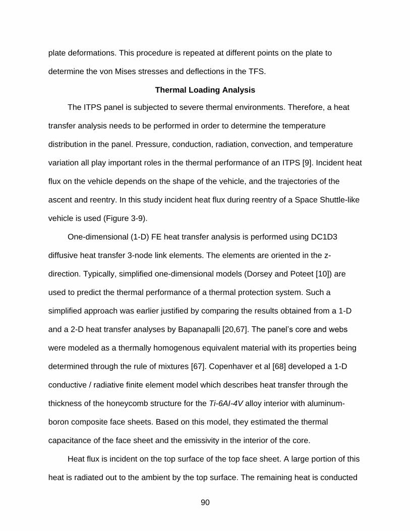
90
plate deformations. This procedure is repeated at different points on the plate to
determine the von Mises stresses and deflections in the TFS.
Thermal Loading Analysis
The ITPS panel is subjected to severe thermal environments. Therefore, a heat
transfer analysis needs to be performed in order to determine the temperature
distribution in the panel. Pressure, conduction, radiation, convection, and temperature
variation all play important roles in the thermal performance of an ITPS [9]. Incident heat
flux on the vehicle depends on the shape of the vehicle, and the trajectories of the
ascent and reentry. In this study incident heat flux during reentry of a Space Shuttle-like
vehicle is used (Figure 3-9).
One-dimensional (1-D) FE heat transfer analysis is performed using DC1D3
diffusive heat transfer 3-node link elements. The elements are oriented in the z-
direction. Typically, simplified one-dimensional models (Dorsey and Poteet [10]) are
used to predict the thermal performance of a thermal protection system. Such a
simplified approach was earlier justified by comparing the results obtained from a 1-D
and a 2-D heat transfer analyses by Bapanapalli [20,67]. The panel‟s core and webs
were modeled as a thermally homogenous equivalent material with its properties being
determined through the rule of mixtures [67]. Copenhaver et al [68] developed a 1-D
conductive / radiative finite element model which describes heat transfer through the
thickness of the honeycomb structure for the Ti-6AI-4V alloy interior with aluminum-
boron composite face sheets. Based on this model, they estimated the thermal
capacitance of the face sheet and the emissivity in the interior of the core.
Heat flux is incident on the top surface of the top face sheet. A large portion of this
heat is radiated out to the ambient by the top surface. The remaining heat is conducted
91
into the ITPS. Also the bottom surface of the bottom face sheet is assumed to be
perfectly insulated. This is the worst case scenario where the bottom face sheet
temperature would rise to a maximum as it cannot dissipate the heat. It is also assumed
that there is no lateral heat flow out of the unit cell; that is, the heat flux incident on a
unit cell is completely absorbed by that unit cell only. Similar model and boundary
conditions were chosen by Bapanapalli et al [20]. It was found that the stresses in the
ITPS panel are maximum when the average temperature gradient through the panel
thickness is at its severest and is the major driver of thermal stresses (Figure 3-10).
In Martinez et al [21, 69], a micromechanical method is developed analytically to
calculate the equivalent thermal forces and moments for a given temperature
distribution. The method was demonstrated by calculating stresses in a sandwich panel
subjected to a temperature distribution described by a quartic polynomial in the
thickness direction. The results for stresses are compared with that from a three-
dimensional finite element analysis. As mentioned earlier, the analytical method has
limitations and hence we chose the finite element based homogenization method in the
present study.
Thermal force and moments are caused in the ITPS panel when there is through-
the-thickness temperature gradient. The thermo-elastic laminate constitutive relations
are given as,
T
o
T
N NK
M M
(3-1)
In Equation 3-1, NT and MT are the unit cell‟s thermal force and moment resultants and
moment due to temperature variation through the thickness of the ITPS. The thermal
92
force resultants and moments are equal to the negative of forces and moments that act
on the unit cell when it is completely constrained at its lateral boundary surfaces.
The thermal analysis is broken into two parts. First, the unit cell is constrained to
prevent lateral deformations using periodic boundary conditions and then the through
the thickness temperature distribution is applied to the unit cell (Figure 3-11). The
temperature distribution equation was determined by fitting a quartic polynomial to the
actual temperature distribution. From the stresses in the unit cell the thermal forces (NT)
and thermal moments (MT) are computed (Part i). The nodal forces of the boundary
nodes were determined from the finite element analyses. The force and moment
resultants acting on the unit cell were obtained from the nodal forces using Equation 3-
2.
( )
1
( )
1
1, 1, ( , , ) For the face
1, 1, ( , , ) For the face
tnm
x x x
m
tnm
y y y
m
N M z F a y z x ab
N M z F x b z y ba
(3-2)
where
and
are the nodal forces in the x and y directions at the mth node
and „tn‟ is the total number of nodes on the face. The resultants obtained are the forces
needed to constrain the unit cell during a change in temperature, and they will be equal
to the negative of the thermal forces of the ITPS as can be seen from the thermo-elastic
laminate constitutive relation.
T
o
T
T
T
N NK
M M
NN
MM
(3-3)
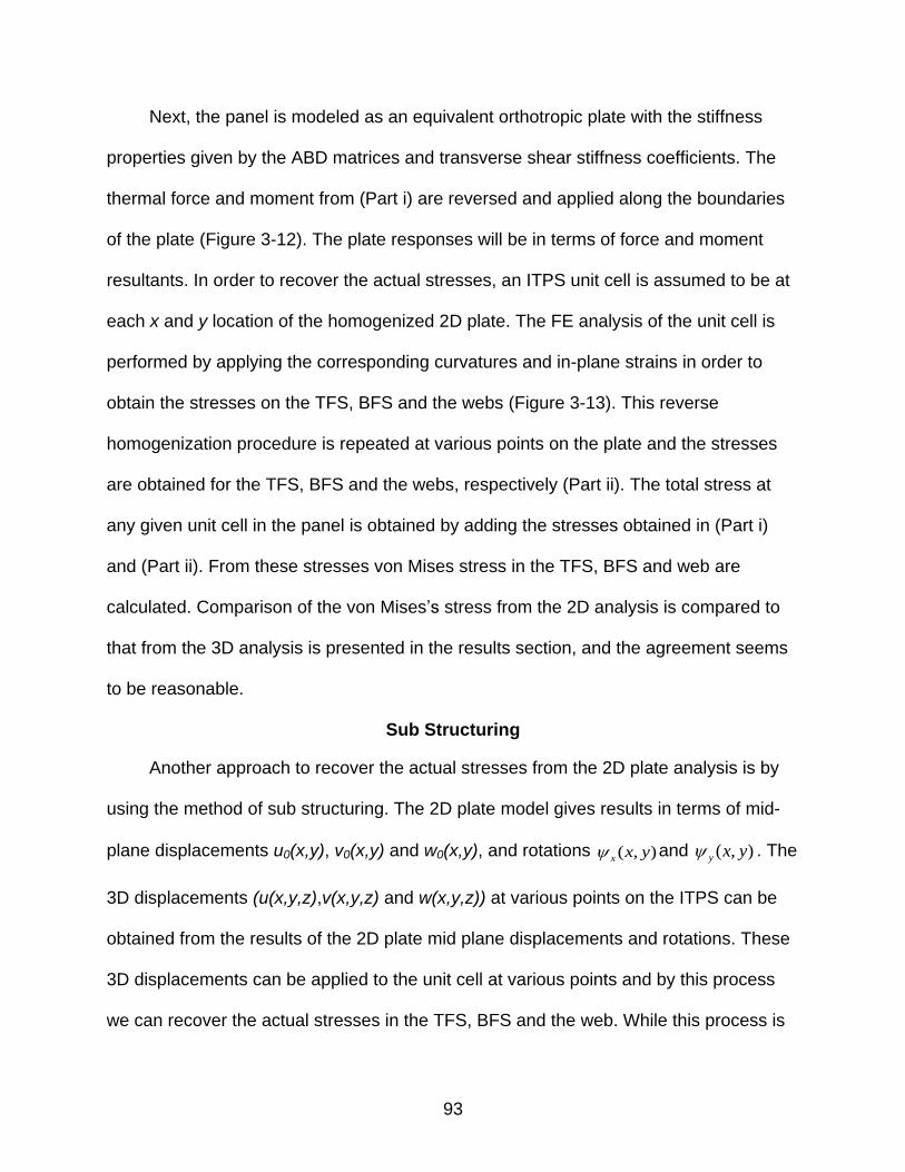
93
Next, the panel is modeled as an equivalent orthotropic plate with the stiffness
properties given by the ABD matrices and transverse shear stiffness coefficients. The
thermal force and moment from (Part i) are reversed and applied along the boundaries
of the plate (Figure 3-12). The plate responses will be in terms of force and moment
resultants. In order to recover the actual stresses, an ITPS unit cell is assumed to be at
each x and y location of the homogenized 2D plate. The FE analysis of the unit cell is
performed by applying the corresponding curvatures and in-plane strains in order to
obtain the stresses on the TFS, BFS and the webs (Figure 3-13). This reverse
homogenization procedure is repeated at various points on the plate and the stresses
are obtained for the TFS, BFS and the webs, respectively (Part ii). The total stress at
any given unit cell in the panel is obtained by adding the stresses obtained in (Part i)
and (Part ii). From these stresses von Mises stress in the TFS, BFS and web are
calculated. Comparison of the von Mises‟s stress from the 2D analysis is compared to
that from the 3D analysis is presented in the results section, and the agreement seems
to be reasonable.
Sub Structuring
Another approach to recover the actual stresses from the 2D plate analysis is by
using the method of sub structuring. The 2D plate model gives results in terms of mid-
plane displacements u0(x,y), v0(x,y) and w0(x,y), and rotations ( , )x x y and ( , )y x y . The
3D displacements (u(x,y,z),v(x,y,z) and w(x,y,z)) at various points on the ITPS can be
obtained from the results of the 2D plate mid plane displacements and rotations. These
3D displacements can be applied to the unit cell at various points and by this process
we can recover the actual stresses in the TFS, BFS and the web. While this process is
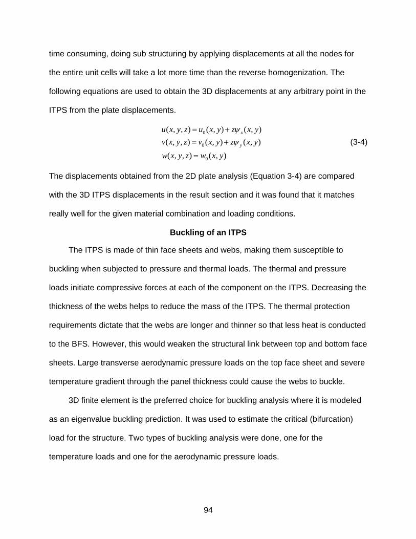
94
time consuming, doing sub structuring by applying displacements at all the nodes for
the entire unit cells will take a lot more time than the reverse homogenization. The
following equations are used to obtain the 3D displacements at any arbitrary point in the
ITPS from the plate displacements.
0
0
0
( , , ) ( , ) ( , )
( , , ) ( , ) ( , )
( , , ) ( , )
x
y
u x y z u x y z x y
v x y z v x y z x y
w x y z w x y
(3-4)
The displacements obtained from the 2D plate analysis (Equation 3-4) are compared
with the 3D ITPS displacements in the result section and it was found that it matches
really well for the given material combination and loading conditions.
Buckling of an ITPS
The ITPS is made of thin face sheets and webs, making them susceptible to
buckling when subjected to pressure and thermal loads. The thermal and pressure
loads initiate compressive forces at each of the component on the ITPS. Decreasing the
thickness of the webs helps to reduce the mass of the ITPS. The thermal protection
requirements dictate that the webs are longer and thinner so that less heat is conducted
to the BFS. However, this would weaken the structural link between top and bottom face
sheets. Large transverse aerodynamic pressure loads on the top face sheet and severe
temperature gradient through the panel thickness could cause the webs to buckle.
3D finite element is the preferred choice for buckling analysis where it is modeled
as an eigenvalue buckling prediction. It was used to estimate the critical (bifurcation)
load for the structure. Two types of buckling analysis were done, one for the
temperature loads and one for the aerodynamic pressure loads.
95
For thermal buckling analysis, temperature loads were obtained in the form of
through thickness temperature distributions from the heat transfer problem. The
temperature distributions are cubic polynomials in z. Using these polynomials,
temperature was imposed on each node of the 3-D buckling model. This implies that the
top and bottom face sheet temperatures are uniform throughout the length and width of
the panel. Several 3D thermal buckling analyses were attempted initially and it was
found that every time the corner most webs near the panel edges buckles (Figure 3-14).
Therefore, it was decided to apply sub structuring to the region near the corners using
Equation 3-2. The 3D displacements along the panel boundary of one unit cell length
are obtained from the plate displacements when the plate is subjected to thermal force
and moment resultants. These displacements are applied on to the unit cell and the
temperature distribution is applied on each node of the unit cell obtained from the heat
transfer and a unit cell buckling analysis is done (Figure 3-15). The unit cell thermal
buckling analysis is then compared with the entire 3D ITPS thermal buckling analysis
results.
For pressure buckling analysis, aerodynamic pressure load is applied on the TFS.
Again, several 3D pressure buckling analyses were carried out initially and it was found
that every time a different web buckles as shown from Figure 3-16. Since sub
structuring will not be used in such cases, it was decided to use full 3D eigen value
buckling analysis.
Results
For verification of the effectiveness of the deflections and stress results under the
action of uniform pressure loading and thermal loading for the FE based
homogenization method, consider a corrugated-core sandwich panel unit cell with the
96
following dimensions: p = 25 mm, d = 70 mm, tTF = 1.2 mm, tBF = 7.49 mm, tw = 1.63
mm, θ = 85o. For the 3D FE analysis the 3D panel is assumed to consist of 20 unit cells.
In the following example, the TFS and the web is modeled using Titanium alloy, Ti-6Al-
4V (E1 = 109 GPa and ν = 0.3) and the BFS is modeled using Beryllium alloy (E1 = 290
GPa and and ν = 0.063) [20].
For the 3D panel, only one fourth of the ITPS panel containing half the total
number of unit cells is modeled using the ABAQUS® finite element (FE) software
(Figure 3-17). The model uses approximately a total of 140,000 eight-node shell
elements (S8R). The boundary conditions considered are: fixed vertical displacements
for the bottom face sheet (BFS) (w = 0) and fixed rotations for the top face sheet (TFS)
(θx = θy = 0) on the edges of the panel. On the symmetric edges, symmetric boundary
conditions are used. Similar boundary conditions and modeling procedures are also
referred in Bapanapalli et al [20].
The plate is also modeled using shell elements in ABAQUS® finite element (FE)
software. The model used a total of 33,000 eight-node shell elements (S8R). A simply
supported boundary condition is considered along the boundary of the plate (w = 0)
(Figure 3-18). The plate edges are allowed to move in the horizontal plane. Due to
symmetry only one-fourth of the panel is modeled.
ITPS Out-of-Plane Displacement, Uniform Pressure Load
The 3D ITPS panel was subjected to a uniform pressure loading of 101,325 Pa on
the top face sheet. Similarly, the pressure load is also applied to the homogenized plate
model. Also, the corresponding ABD matrices and the transverse shear stiffness
properties, A44 and A55, is input into the homogenized plate model. The plate out-of-
plane displacements compared well to the 3D BFS out-of-plane displacements.
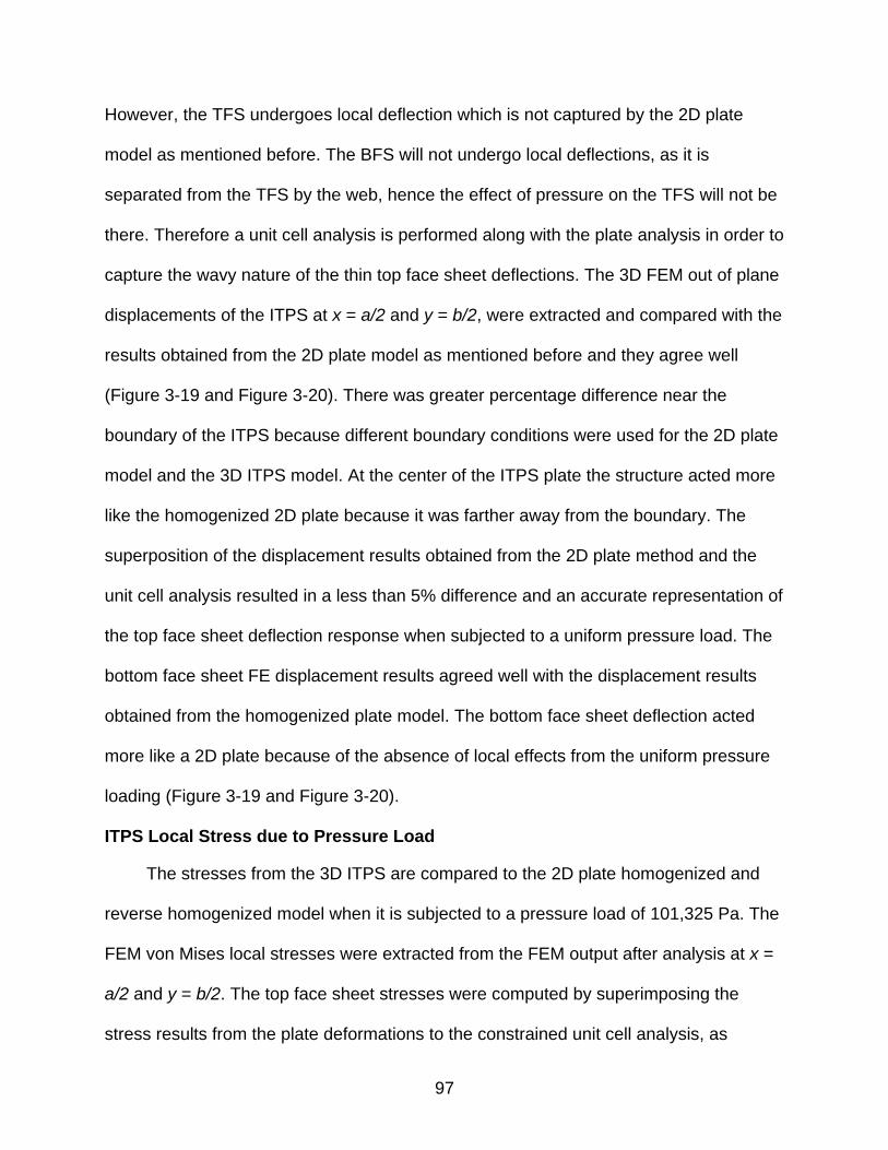
97
However, the TFS undergoes local deflection which is not captured by the 2D plate
model as mentioned before. The BFS will not undergo local deflections, as it is
separated from the TFS by the web, hence the effect of pressure on the TFS will not be
there. Therefore a unit cell analysis is performed along with the plate analysis in order to
capture the wavy nature of the thin top face sheet deflections. The 3D FEM out of plane
displacements of the ITPS at x = a/2 and y = b/2, were extracted and compared with the
results obtained from the 2D plate model as mentioned before and they agree well
(Figure 3-19 and Figure 3-20). There was greater percentage difference near the
boundary of the ITPS because different boundary conditions were used for the 2D plate
model and the 3D ITPS model. At the center of the ITPS plate the structure acted more
like the homogenized 2D plate because it was farther away from the boundary. The
superposition of the displacement results obtained from the 2D plate method and the
unit cell analysis resulted in a less than 5% difference and an accurate representation of
the top face sheet deflection response when subjected to a uniform pressure load. The
bottom face sheet FE displacement results agreed well with the displacement results
obtained from the homogenized plate model. The bottom face sheet deflection acted
more like a 2D plate because of the absence of local effects from the uniform pressure
loading (Figure 3-19 and Figure 3-20).
ITPS Local Stress due to Pressure Load
The stresses from the 3D ITPS are compared to the 2D plate homogenized and
reverse homogenized model when it is subjected to a pressure load of 101,325 Pa. The
FEM von Mises local stresses were extracted from the FEM output after analysis at x =
a/2 and y = b/2. The top face sheet stresses were computed by superimposing the
stress results from the plate deformations to the constrained unit cell analysis, as
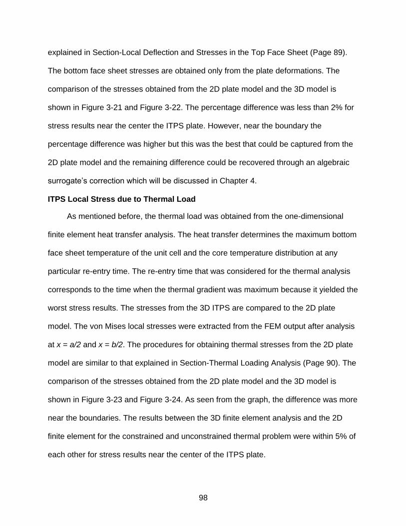
98
explained in Section-Local Deflection and Stresses in the Top Face Sheet (Page 89).
The bottom face sheet stresses are obtained only from the plate deformations. The
comparison of the stresses obtained from the 2D plate model and the 3D model is
shown in Figure 3-21 and Figure 3-22. The percentage difference was less than 2% for
stress results near the center the ITPS plate. However, near the boundary the
percentage difference was higher but this was the best that could be captured from the
2D plate model and the remaining difference could be recovered through an algebraic
surrogate‟s correction which will be discussed in Chapter 4.
ITPS Local Stress due to Thermal Load
As mentioned before, the thermal load was obtained from the one-dimensional
finite element heat transfer analysis. The heat transfer determines the maximum bottom
face sheet temperature of the unit cell and the core temperature distribution at any
particular re-entry time. The re-entry time that was considered for the thermal analysis
corresponds to the time when the thermal gradient was maximum because it yielded the
worst stress results. The stresses from the 3D ITPS are compared to the 2D plate
model. The von Mises local stresses were extracted from the FEM output after analysis
at x = a/2 and x = b/2. The procedures for obtaining thermal stresses from the 2D plate
model are similar to that explained in Section-Thermal Loading Analysis (Page 90). The
comparison of the stresses obtained from the 2D plate model and the 3D model is
shown in Figure 3-23 and Figure 3-24. As seen from the graph, the difference was more
near the boundaries. The results between the 3D finite element analysis and the 2D
finite element for the constrained and unconstrained thermal problem were within 5% of
each other for stress results near the center of the ITPS plate.
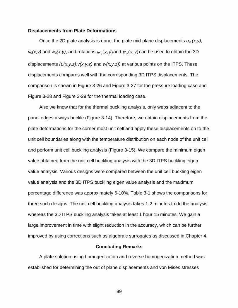
99
Displacements from Plate Deformations
Once the 2D plate analysis is done, the plate mid-plane displacements u0 (x,y),
v0(x,y) and w0(x,y), and rotations ( , )x x y and ( , )y x y can be used to obtain the 3D
displacements (u(x,y,z),v(x,y,z) and w(x,y,z)) at various points on the ITPS. These
displacements compares well with the corresponding 3D ITPS displacements. The
comparison is shown in Figure 3-26 and Figure 3-27 for the pressure loading case and
Figure 3-28 and Figure 3-29 for the thermal loading case.
Also we know that for the thermal buckling analysis, only webs adjacent to the
panel edges always buckle (Figure 3-14). Therefore, we obtain displacements from the
plate deformations for the corner most unit cell and apply these displacements on to the
unit cell boundaries along with the temperature distribution on each node of the unit cell
and perform unit cell buckling analysis (Figure 3-15). We compare the minimum eigen
value obtained from the unit cell buckling analysis with the 3D ITPS buckling eigen
value analysis. Various designs were compared between the unit cell buckling eigen
value analysis and the 3D ITPS buckling eigen value analysis and the maximum
percentage difference was approximately 6-10%. Table 3-1 shows the comparisons for
three such designs. The unit cell buckling analysis takes 1-2 minutes to do the analysis
whereas the 3D ITPS buckling analysis takes at least 1 hour 15 minutes. We gain a
large improvement in time with slight reduction in the accuracy, which can be further
improved by using corrections such as algebraic surrogates as discussed in Chapter 4.
Concluding Remarks
A plate solution using homogenization and reverse homogenization method was
established for determining the out of plane displacements and von Mises stresses
100
under thermal and pressure loads. The plate out of plane displacement results are
within 5% difference from the 3D FEM results for the pressure loading case. However,
the percentage difference of the von Mises stress between the 3D analysis and the 2D
analysis was higher and was greater at the boundary of the ITPS panel for both the
pressure and thermal loading case. The majority of stresses at points away from the
boundaries can be approximated well by the 2D plate analysis. Further for the pressure
loading case, the BFS acts more like a 2D plate as there was no local effect of pressure
load as it was being applied on the TFS. We also compared the buckling unit cell eigen
value analysis with the 3D ITPS buckling analysis under thermal loads and the
maximum percentage difference was found to be approximately between 6-10%. Unit
cell buckling analysis is not possible for the case of pressure load because for different
designs, different webs buckle.
Though there were differences between the 2D plate analysis and 3D ITPS
analysis in the prediction of stresses and deflections, this difficulty will be resolved by
fitting the low-fidelity 2D finite element model with high quality surrogate, which will then
be corrected by the use of a small number of high fidelity 3D finite element analyses.
This approach is known as multi-fidelity or variable-complexity modeling, allows the use
of fewer analysis of the 3D high fidelity, for a given accuracy. This multi-fidelity response
surface technique will be used in our design optimization and is explained in detail in
Chapter 4.
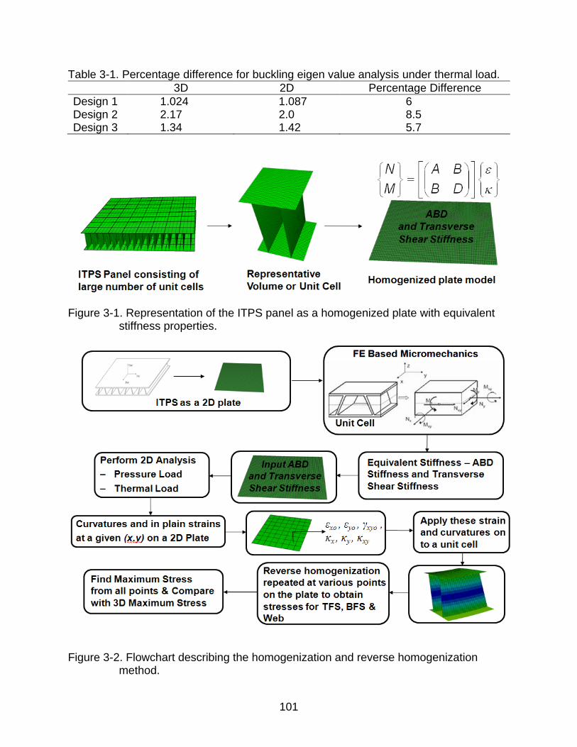
101
Table 3-1. Percentage difference for buckling eigen value analysis under thermal load.
3D 2D Percentage Difference
Design 1 1.024 1.087 6 Design 2 2.17 2.0 8.5 Design 3 1.34 1.42 5.7
Figure 3-1. Representation of the ITPS panel as a homogenized plate with equivalent stiffness properties.
Figure 3-2. Flowchart describing the homogenization and reverse homogenization
method.
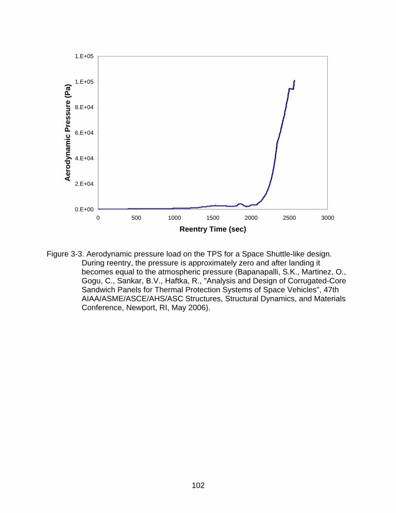
102
Figure 3-3. Aerodynamic pressure load on the TPS for a Space Shuttle-like design. During reentry, the pressure is approximately zero and after landing it becomes equal to the atmospheric pressure (Bapanapalli, S.K., Martinez, O., Gogu, C., Sankar, B.V., Haftka, R., "Analysis and Design of Corrugated-Core Sandwich Panels for Thermal Protection Systems of Space Vehicles", 47th AIAA/ASME/ASCE/AHS/ASC Structures, Structural Dynamics, and Materials Conference, Newport, RI, May 2006).
0.E+00
2.E+04
4.E+04
6.E+04
8.E+04
1.E+05
1.E+05
0 500 1000 1500 2000 2500 3000
Reentry Time (sec)
Aero
dyn
am
ic P
ressu
re (
Pa)
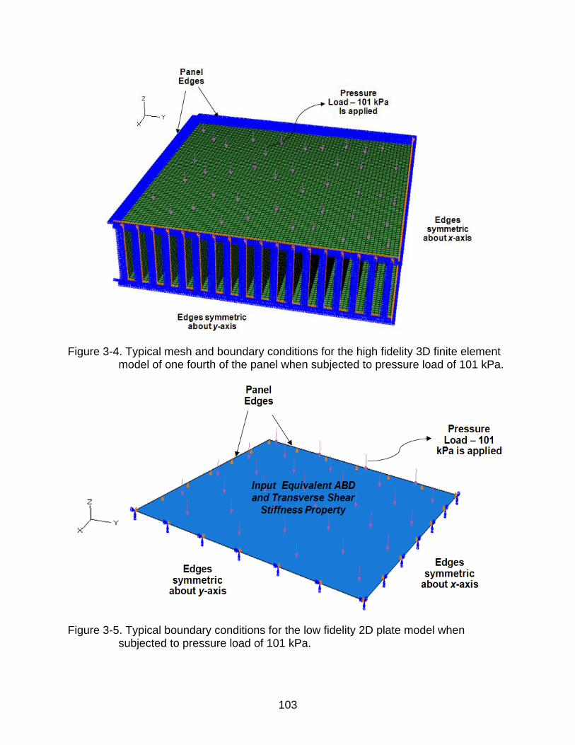
103
Figure 3-4. Typical mesh and boundary conditions for the high fidelity 3D finite element model of one fourth of the panel when subjected to pressure load of 101 kPa.
Figure 3-5. Typical boundary conditions for the low fidelity 2D plate model when subjected to pressure load of 101 kPa.
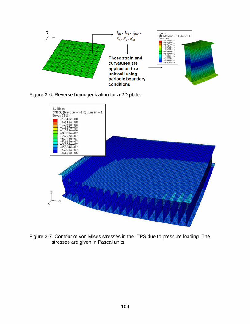
104
Figure 3-6. Reverse homogenization for a 2D plate.
Figure 3-7. Contour of von Mises stresses in the ITPS due to pressure loading. The stresses are given in Pascal units.
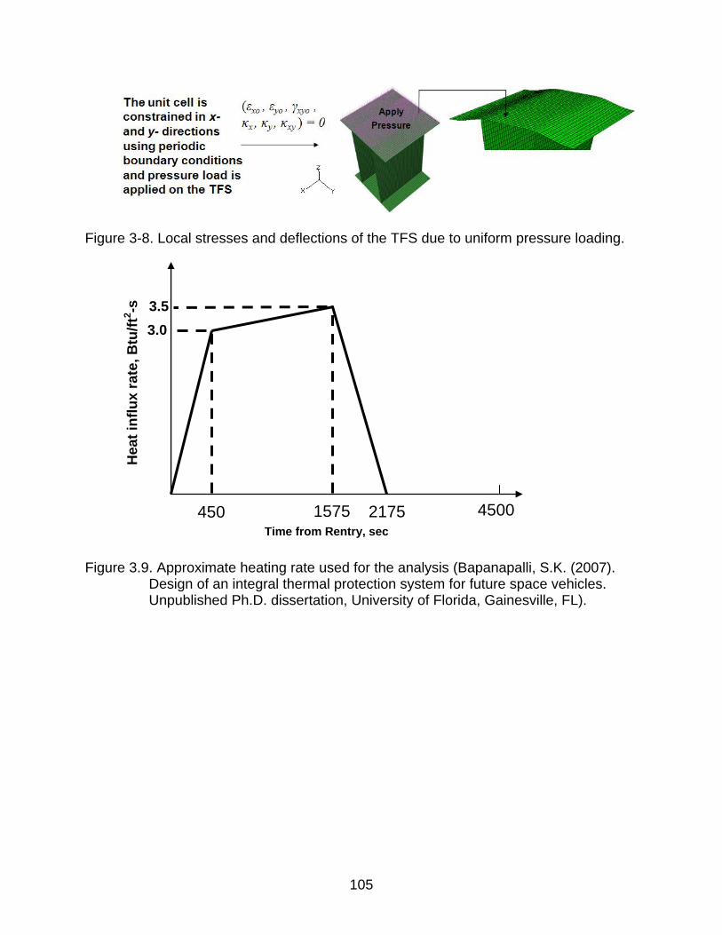
105
Figure 3-8. Local stresses and deflections of the TFS due to uniform pressure loading.
Figure 3.9. Approximate heating rate used for the analysis (Bapanapalli, S.K. (2007). Design of an integral thermal protection system for future space vehicles. Unpublished Ph.D. dissertation, University of Florida, Gainesville, FL).
450 2175 1575 4500
Time from Rentry, sec
Heat
infl
ux r
ate
, B
tu/f
t2-s
3.0
3.5
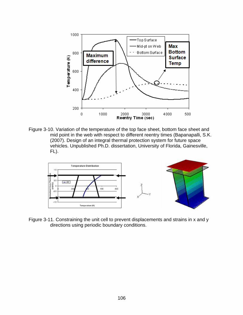
106
Figure 3-10. Variation of the temperature of the top face sheet, bottom face sheet and mid point in the web with respect to different reentry times (Bapanapalli, S.K. (2007). Design of an integral thermal protection system for future space vehicles. Unpublished Ph.D. dissertation, University of Florida, Gainesville, FL).
Figure 3-11. Constraining the unit cell to prevent displacements and strains in x and y directions using periodic boundary conditions.
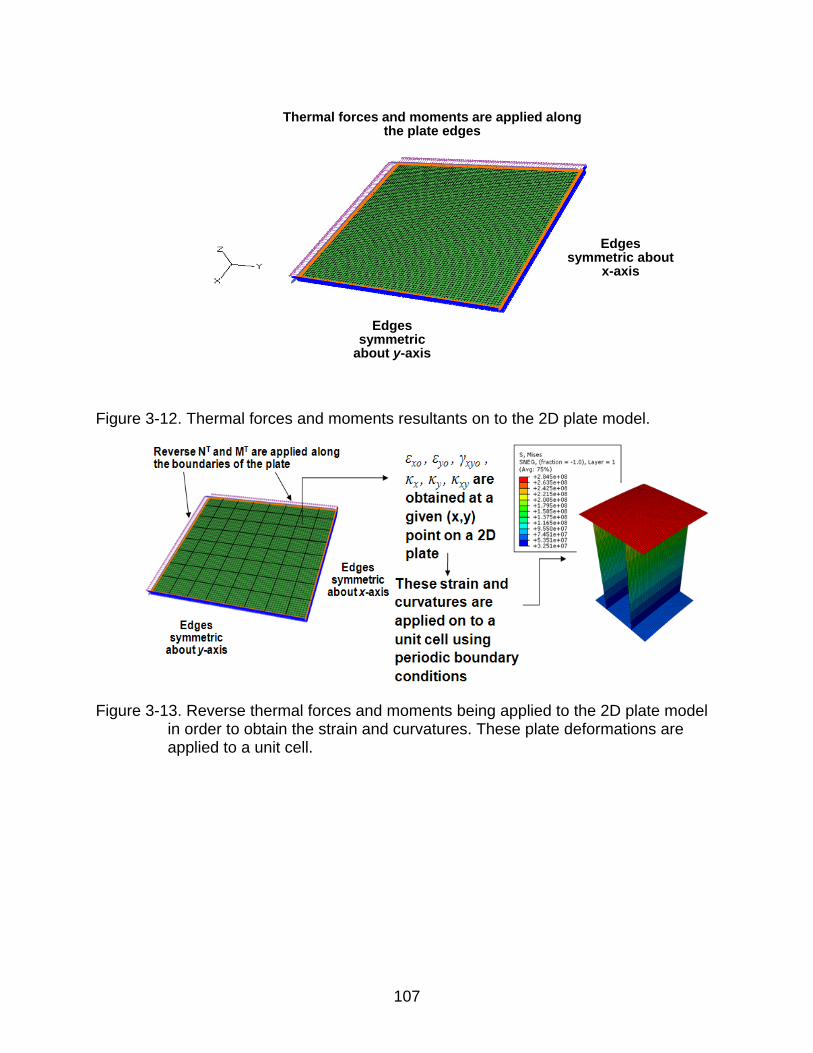
107
Figure 3-12. Thermal forces and moments resultants on to the 2D plate model.
Figure 3-13. Reverse thermal forces and moments being applied to the 2D plate model in order to obtain the strain and curvatures. These plate deformations are applied to a unit cell.
Edges symmetric
about y-axis
Edges symmetric about
x-axis
Thermal forces and moments are applied along the plate edges
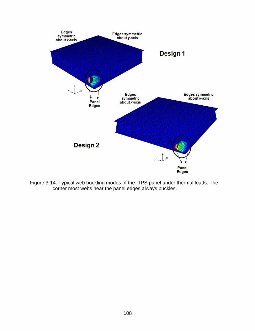
108
Figure 3-14. Typical web buckling modes of the ITPS panel under thermal loads. The corner most webs near the panel edges always buckles.
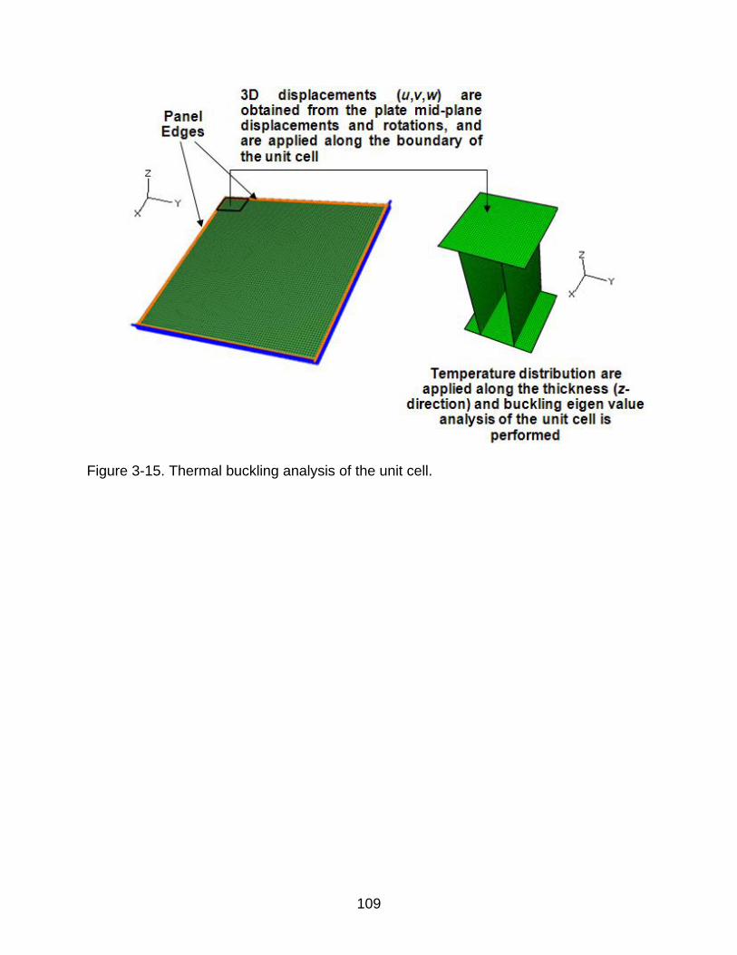
109
Figure 3-15. Thermal buckling analysis of the unit cell.
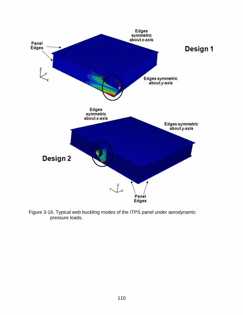
110
Figure 3-16. Typical web buckling modes of the ITPS panel under aerodynamic pressure loads.
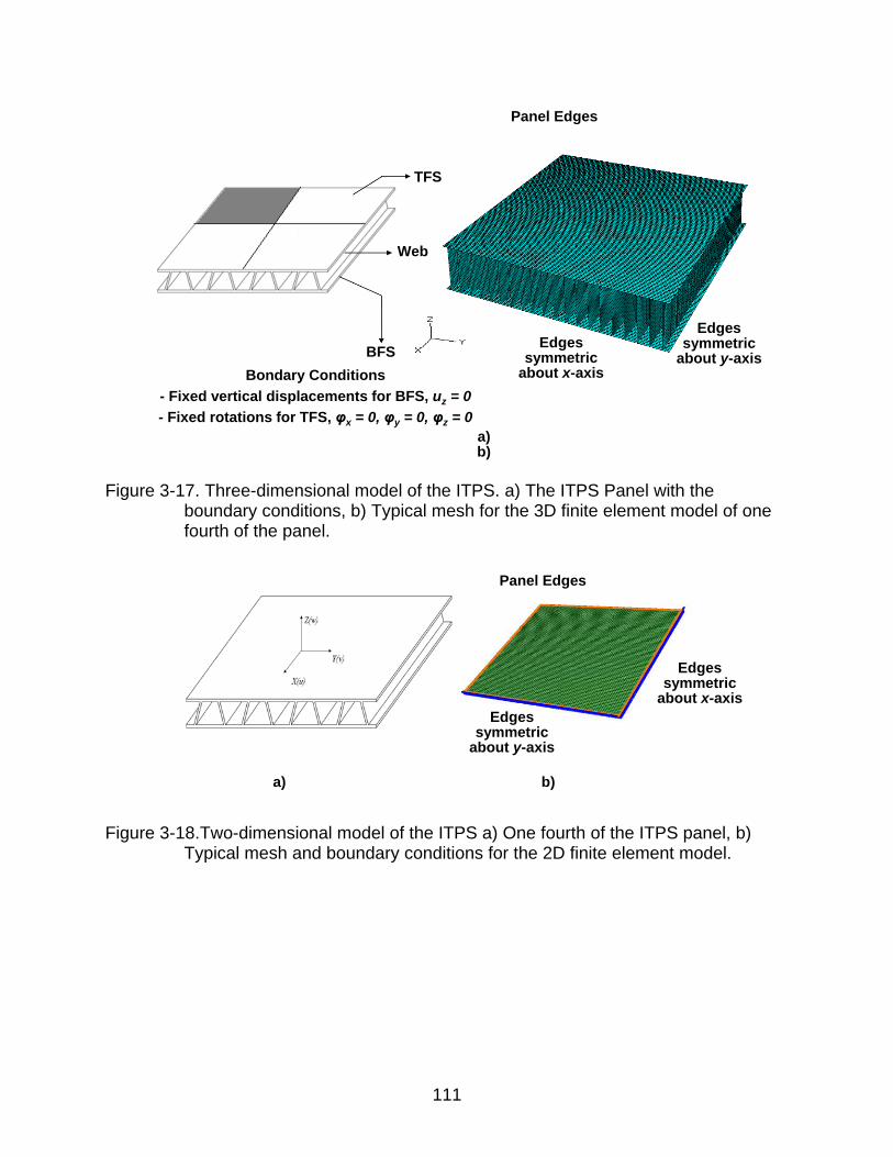
111
Figure 3-17. Three-dimensional model of the ITPS. a) The ITPS Panel with the boundary conditions, b) Typical mesh for the 3D finite element model of one fourth of the panel.
Figure 3-18.Two-dimensional model of the ITPS a) One fourth of the ITPS panel, b) Typical mesh and boundary conditions for the 2D finite element model.
Panel Edges
Edges symmetric
about y-axis Edges
symmetric about x-axis
a) b)
TFS
Web
BFS
Bondary Conditions
- Fixed vertical displacements for BFS, uz = 0
- Fixed rotations for TFS, φx = 0, φy = 0, φz = 0
a) b)
Panel Edges
Edges symmetric
about x-axis
Edges symmetric
about y-axis
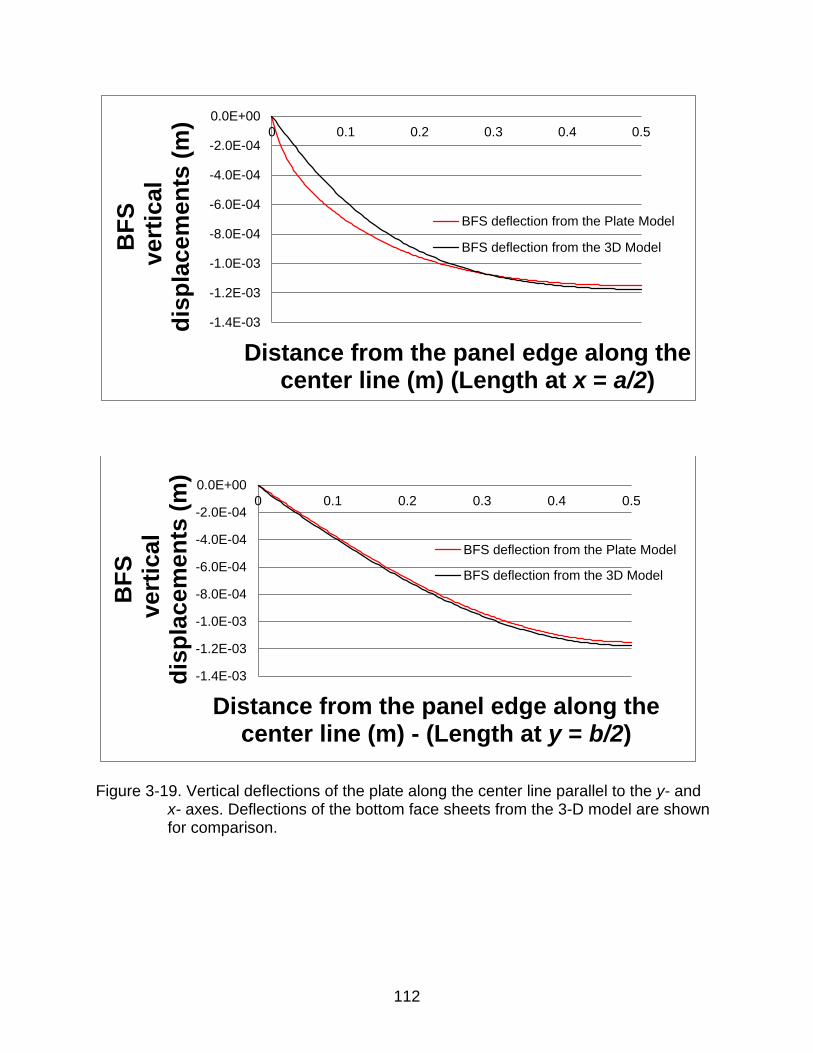
112
Figure 3-19. Vertical deflections of the plate along the center line parallel to the y- and x- axes. Deflections of the bottom face sheets from the 3-D model are shown for comparison.
-1.4E-03
-1.2E-03
-1.0E-03
-8.0E-04
-6.0E-04
-4.0E-04
-2.0E-04
0.0E+00
0 0.1 0.2 0.3 0.4 0.5B
FS
v
ert
ical
dis
pla
cem
en
ts (
m)
Distance from the panel edge along the center line (m) (Length at x = a/2)
BFS deflection from the Plate Model
BFS deflection from the 3D Model
-1.4E-03
-1.2E-03
-1.0E-03
-8.0E-04
-6.0E-04
-4.0E-04
-2.0E-04
0.0E+00
0 0.1 0.2 0.3 0.4 0.5
BF
S
vert
ical
dis
pla
cem
en
ts (
m)
Distance from the panel edge along the center line (m) - (Length at y = b/2)
BFS deflection from the Plate Model
BFS deflection from the 3D Model
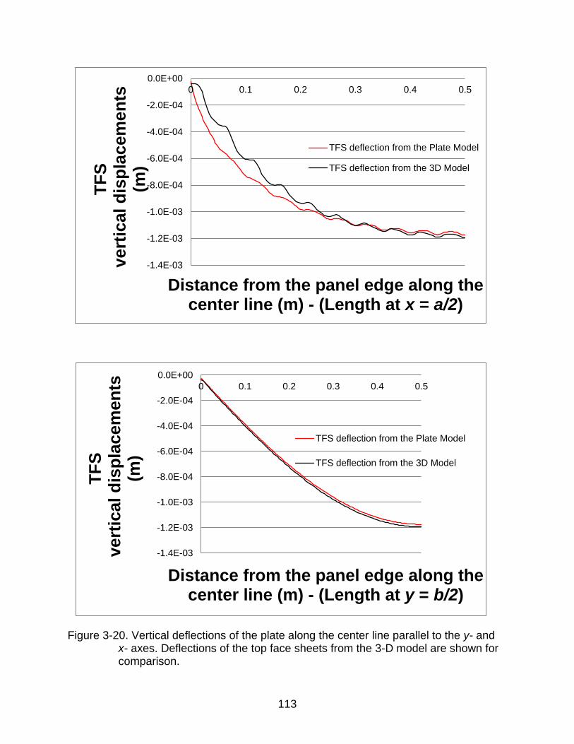
113
Figure 3-20. Vertical deflections of the plate along the center line parallel to the y- and x- axes. Deflections of the top face sheets from the 3-D model are shown for comparison.
-1.4E-03
-1.2E-03
-1.0E-03
-8.0E-04
-6.0E-04
-4.0E-04
-2.0E-04
0.0E+00
0 0.1 0.2 0.3 0.4 0.5
TF
S
vert
ical
dis
pla
cem
en
ts
(m)
Distance from the panel edge along the center line (m) - (Length at x = a/2)
TFS deflection from the Plate Model
TFS deflection from the 3D Model
-1.4E-03
-1.2E-03
-1.0E-03
-8.0E-04
-6.0E-04
-4.0E-04
-2.0E-04
0.0E+00
0 0.1 0.2 0.3 0.4 0.5
TF
S
vert
ica
l d
isp
lacem
en
ts
(m)
Distance from the panel edge along the center line (m) - (Length at y = b/2)
TFS deflection from the Plate Model
TFS deflection from the 3D Model
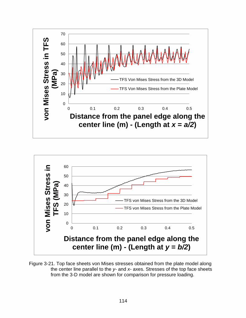
114
Figure 3-21. Top face sheets von Mises stresses obtained from the plate model along the center line parallel to the y- and x- axes. Stresses of the top face sheets from the 3-D model are shown for comparison for pressure loading.
0
10
20
30
40
50
60
70
0 0.1 0.2 0.3 0.4 0.5
vo
n M
ises S
tress
in
TF
S
(MP
a)
Distance from the panel edge along the center line (m) - (Length at x = a/2)
TFS Von Mises Stress from the 3D Model
TFS Von Mises Stress from the Plate Model
0
10
20
30
40
50
60
0 0.1 0.2 0.3 0.4 0.5vo
n M
ises S
tress
in
T
FS
(M
Pa
)
Distance from the panel edge along the center line (m) - (Length at y = b/2)
TFS von Mises Stress from the 3D Model
TFS von Mises Stress from the Plate Model
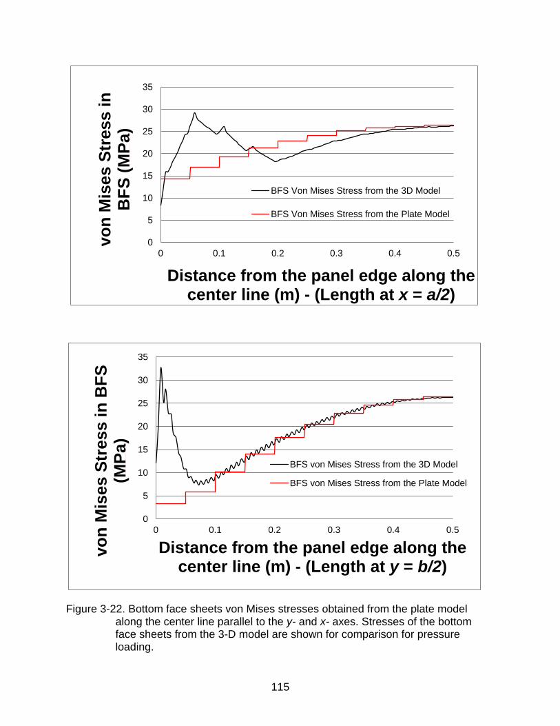
115
Figure 3-22. Bottom face sheets von Mises stresses obtained from the plate model along the center line parallel to the y- and x- axes. Stresses of the bottom face sheets from the 3-D model are shown for comparison for pressure loading.
0
5
10
15
20
25
30
35
0 0.1 0.2 0.3 0.4 0.5
vo
n M
ises S
tress
in
B
FS
(M
Pa
)
Distance from the panel edge along the center line (m) - (Length at x = a/2)
BFS Von Mises Stress from the 3D Model
BFS Von Mises Stress from the Plate Model
0
5
10
15
20
25
30
35
0 0.1 0.2 0.3 0.4 0.5
vo
n M
ise
s S
tress
in
BF
S
(MP
a)
Distance from the panel edge along the center line (m) - (Length at y = b/2)
BFS von Mises Stress from the 3D Model
BFS von Mises Stress from the Plate Model
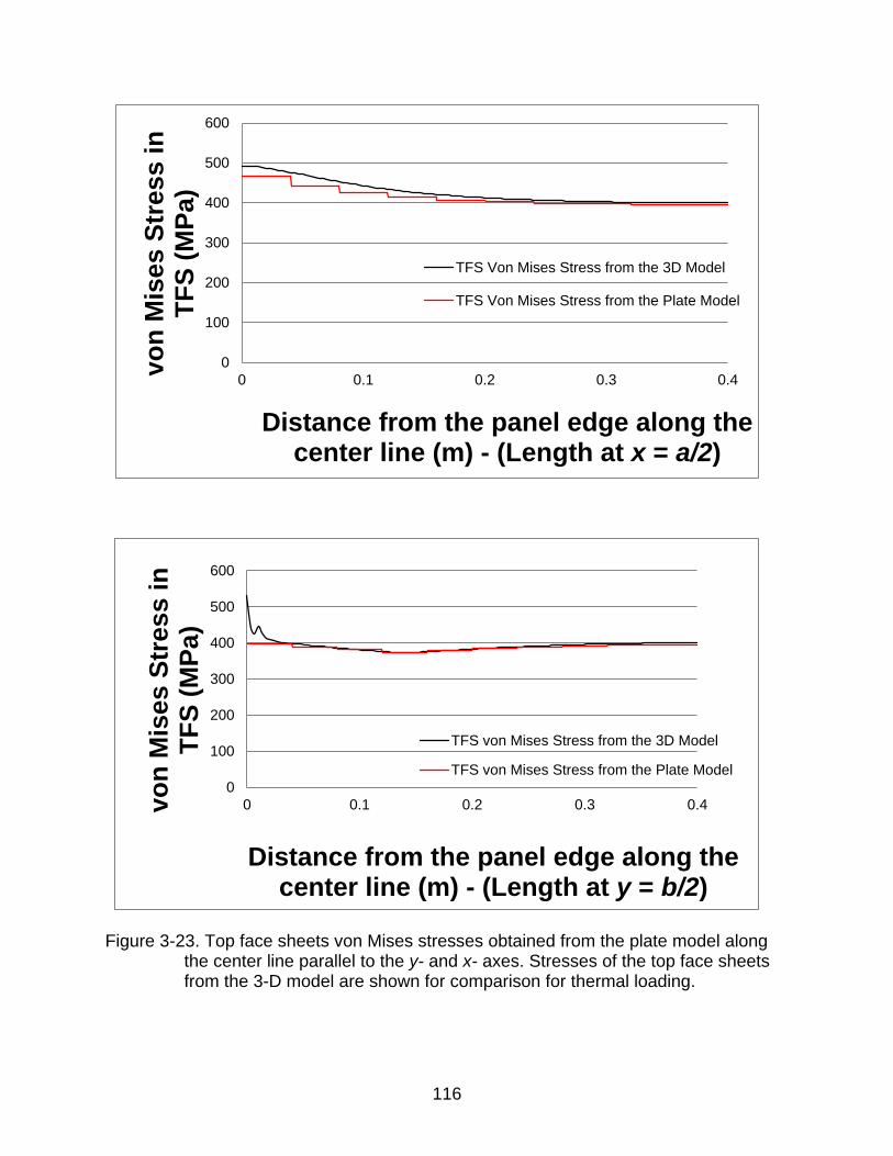
116
Figure 3-23. Top face sheets von Mises stresses obtained from the plate model along the center line parallel to the y- and x- axes. Stresses of the top face sheets from the 3-D model are shown for comparison for thermal loading.
0
100
200
300
400
500
600
0 0.1 0.2 0.3 0.4
vo
n M
ises S
tress
in
T
FS
(M
Pa)
Distance from the panel edge along the center line (m) - (Length at x = a/2)
TFS Von Mises Stress from the 3D Model
TFS Von Mises Stress from the Plate Model
0
100
200
300
400
500
600
0 0.1 0.2 0.3 0.4vo
n M
ises S
tress
in
T
FS
(M
Pa)
Distance from the panel edge along the center line (m) - (Length at y = b/2)
TFS von Mises Stress from the 3D Model
TFS von Mises Stress from the Plate Model
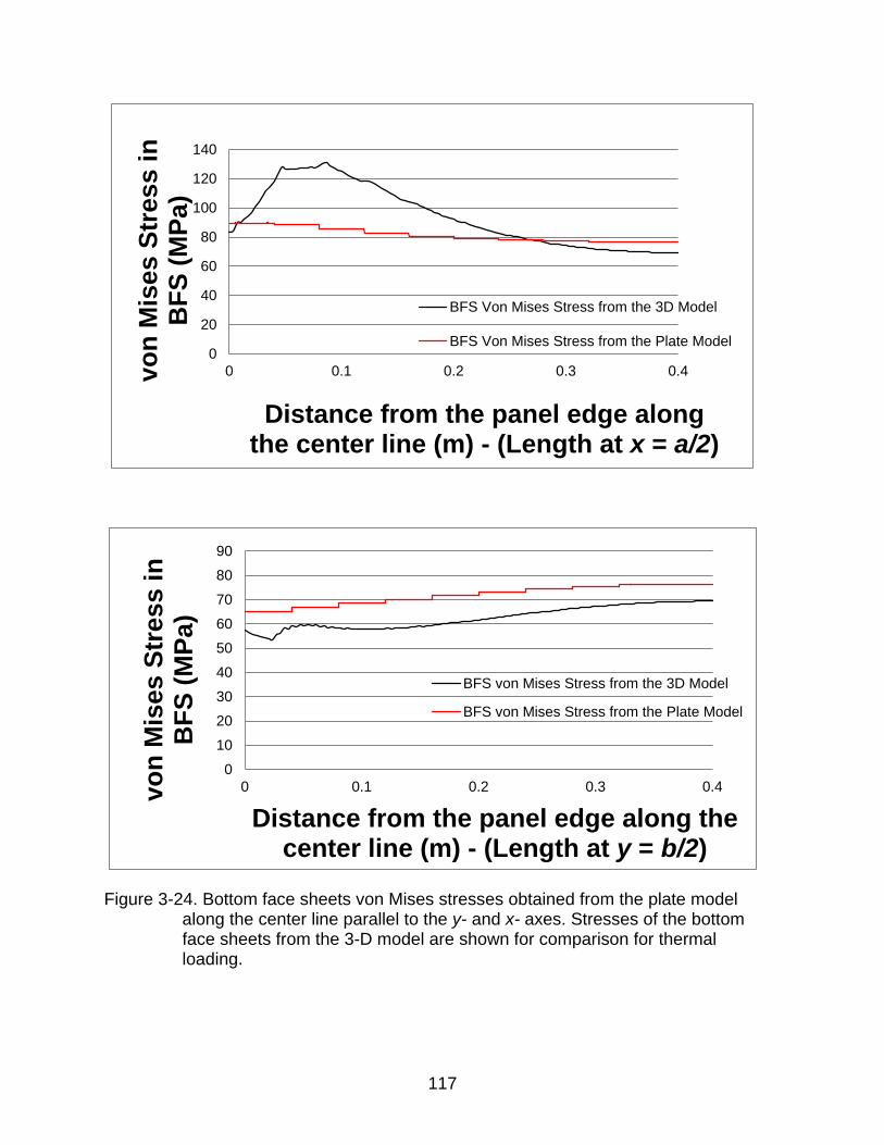
117
Figure 3-24. Bottom face sheets von Mises stresses obtained from the plate model along the center line parallel to the y- and x- axes. Stresses of the bottom face sheets from the 3-D model are shown for comparison for thermal loading.
0
20
40
60
80
100
120
140
0 0.1 0.2 0.3 0.4vo
n M
ises S
tress
in
B
FS
(M
Pa)
Distance from the panel edge along the center line (m) - (Length at x = a/2)
BFS Von Mises Stress from the 3D Model
BFS Von Mises Stress from the Plate Model
0
10
20
30
40
50
60
70
80
90
0 0.1 0.2 0.3 0.4vo
n M
ise
s S
tre
ss
in
B
FS
(M
Pa)
Distance from the panel edge along the center line (m) - (Length at y = b/2)
BFS von Mises Stress from the 3D Model
BFS von Mises Stress from the Plate Model
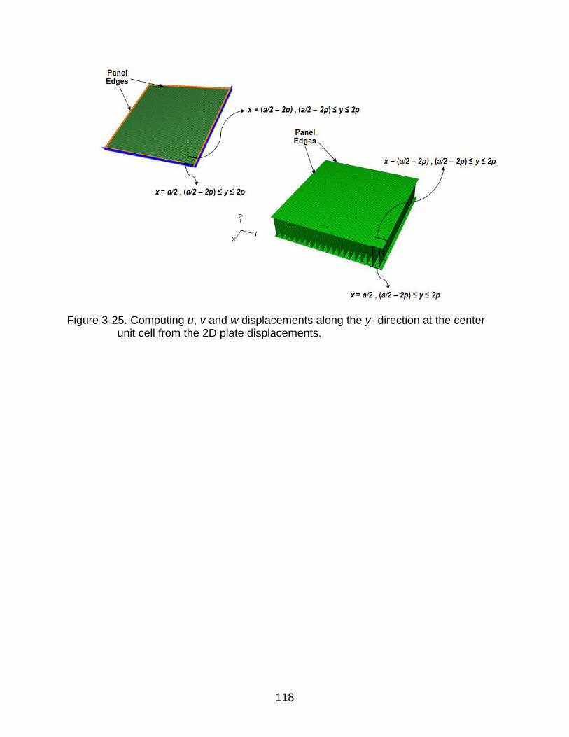
118
Figure 3-25. Computing u, v and w displacements along the y- direction at the center unit cell from the 2D plate displacements.
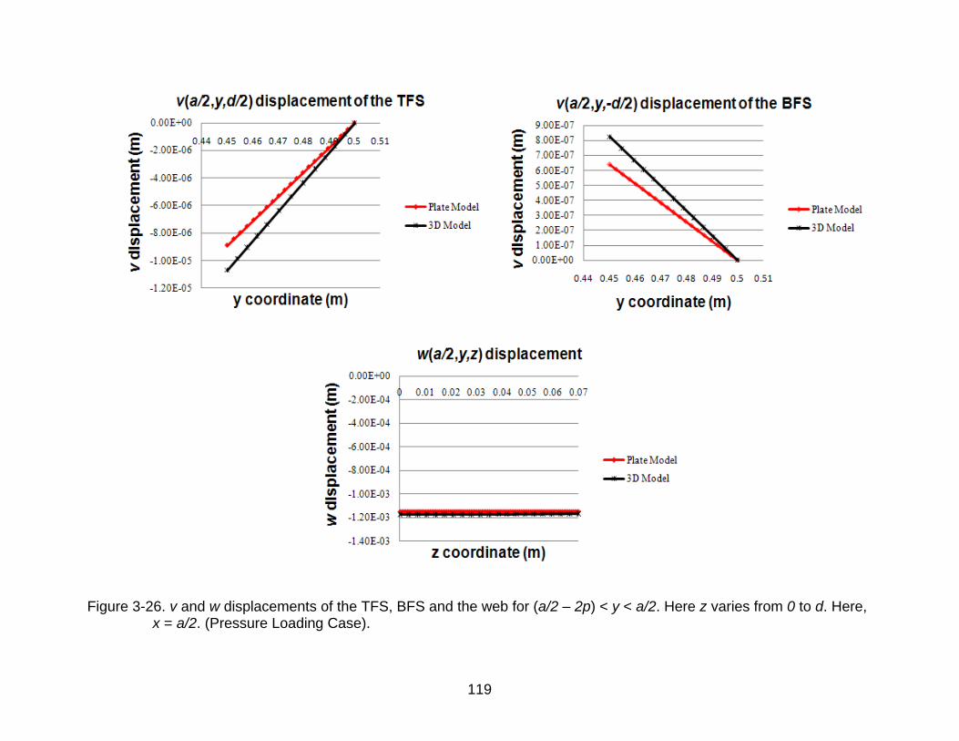
119
Figure 3-26. v and w displacements of the TFS, BFS and the web for (a/2 – 2p) < y < a/2. Here z varies from 0 to d. Here, x = a/2. (Pressure Loading Case).
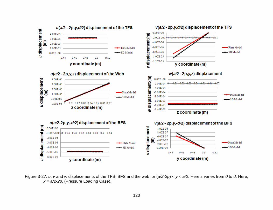
120
Figure 3-27. u, v and w displacements of the TFS, BFS and the web for (a/2-2p) < y < a/2. Here z varies from 0 to d. Here, x = a/2-2p. (Pressure Loading Case).
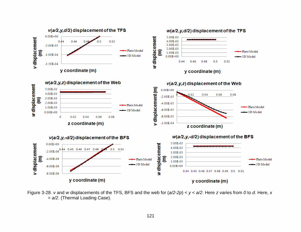
121
Figure 3-28. v and w displacements of the TFS, BFS and the web for (a/2-2p) < y < a/2. Here z varies from 0 to d. Here, x = a/2. (Thermal Loading Case).
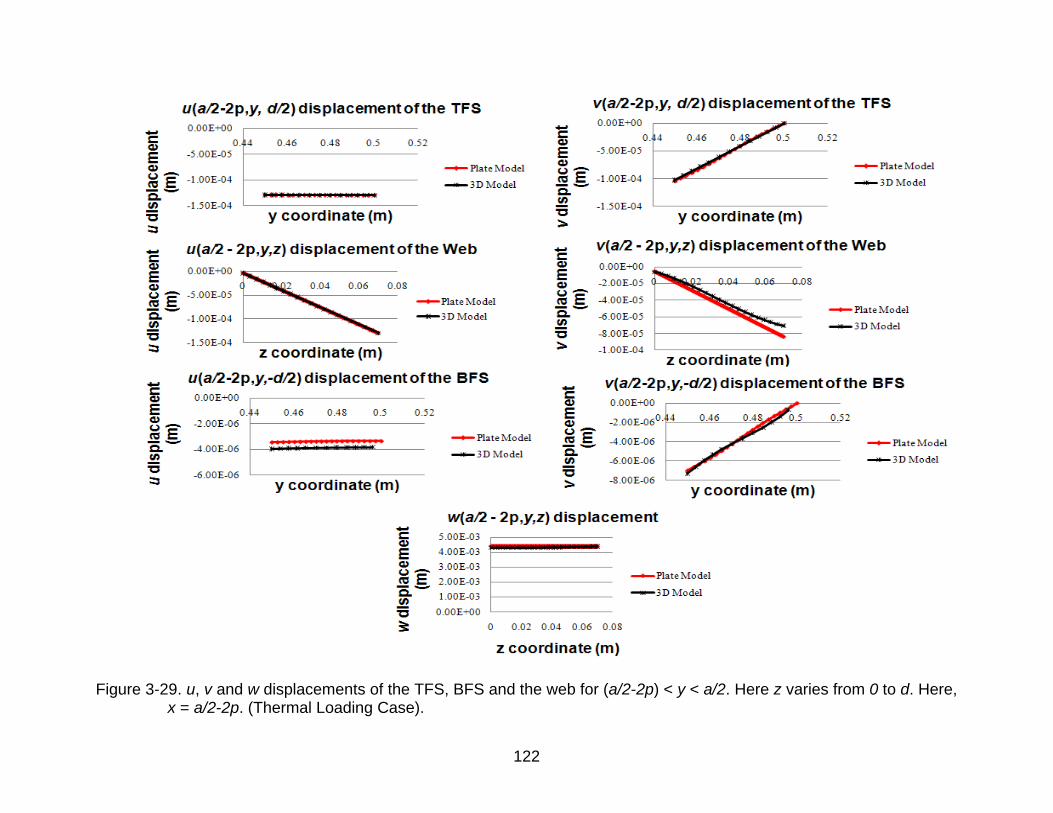
122
Figure 3-29. u, v and w displacements of the TFS, BFS and the web for (a/2-2p) < y < a/2. Here z varies from 0 to d. Here, x = a/2-2p. (Thermal Loading Case).
123
CHAPTER 4 MULTI-FIDELITY DESIGN AND OPTIMIZATION
ITPS is a key technology for reducing the cost of reusable launch vehicles, offering
the combination of increased durability and competitive weights when compared to
other systems. Accurate sizing of ITPS requires combined thermal and structural
analysis [22]. The TPS and the underlying load bearing structure have various
contradictory requirements, which need to be reconciled, in order to find a feasible
solution. This is only possible by making the design process as an optimization problem.
Further, ITPS will occupy a huge area on the vehicle exteriors and forms a major part of
the launch weight. Therefore, material selection, geometric parameters and constraints
all contribute to the total mass of the ITPS. The objective of the process is to make the
structure as light as possible and at the same time it should fulfill all the functions
required of the ITPS.
In [22, 10], the critical functions of an ITPS that have a potential influence on the
design were taken into account. Since the main goal is to reduce the weight of the ITPS,
the obvious choice for the objective would be mass per unit area of the ITPS panel, M.
The optimization problem is stated as minimizing the mass per unit area of the panel
while satisfying various constraints as given below.
Maximum temperature of the bottom face-sheet: The temperature of the underlying structure must at all times be maintained below acceptable limits.
Maximum global/local deflection of the top face-sheet: The maximum deflection should be within acceptable limits to maintain the aerodynamic shape of the spacecraft. The limits are imposed to prevent premature transition from laminar to turbulent flow, which could significantly increase surface heating. Global deflection refers to the deflection of the whole TPS panel while local deflection refers to dimples that can occur in the unsupported section of the top face sheet.
Stresses in the panel: In order to maintain structural integrity the stresses in the panel should be within allowable limits. The loads on the TPS panel include
124
temperature loads that create bending stresses, pressure loads, and in-plane loads from the airframe. Von Mises criterion for yielding is used for metallic structures, while Tsai-Wu failure theory will be used for composite structures.
Thermal/mechanical buckling: Buckling could be global or local. Global buckling is the event when the whole TPS panel buckles, while local buckling is the event when the thin face-sheets or web buckles locally under the loads.
The relation between the geometric parameters and the constraints can be
obtained by using either the 2D FE procedures that were outlined in the previous
chapters or using a complete 3D FE analysis. There is also a third approach where we
can combine the inexpensive 2D FE approach (takes approximately 10 minutes) with
the 3D FE expensive analysis (takes approximately 60-75 minutes) by generating the
multi-fidelity surrogates of the constraints which usually allows use of significantly fewer
3D high fidelity analyses for a given accuracy. This multi-fidelity design approach is
explained in detail in the next section. The optimization problem was performed by
using the MATLAB ® optimization function fmincon(), which is a built-in MATLAB ®
optimization function that optimizes an objective function through a Sequential
Quadratic Programming algorithm (SQP) [83]. The optimization process was carried out
100 times with a different starting point at each optimization and the design with the
lowest weight was chosen as the optimized design.
Multi-Fidelity Design
The problem of optimizing with high cost models is common to many engineering
design problems. The design of an ITPS is a challenging task, because the requirement
of a load bearing structure and a TPS are often conflicting. However, as the structure is
subjected to complex loads like thermal and pressure, the computational time and effort
for a 3D FE analysis increase substantially.
125
Bapanapalli et al [20] developed an optimization procedure to find the optimal
design having minimum mass and satisfying all the constraints. The procedure used 3D
FE analysis to construct response surface approximations (RSAs) for the critical
constraints, including maximum bottom face sheet temperature, maximum deflection,
maximum stresses and buckling loads. The RSAs obtained were of high fidelity;
however they required large computational time. The cost of generating these response
surfaces is high and it increases by an order of magnitude when uncertainties are taken
into account and added as additional variables for obtaining a robust design.
Martinez et al [21] developed an analytical model of the ITPS based on
homogenization of the panel for calculating displacements and stresses. This model,
though relatively inexpensive, was not accurate enough for design optimization.
Therefore in Sharma et al [70], these two models were combined into a multi-fidelity
model, and maximum stresses and maximum deflection in the top face-sheet of the
ITPS structure were calculated under pressure loads. The paper demonstrated that it is
possible to construct the RSA for the various constraints that will be used in the
optimization of ITPS at higher accuracy and low computational cost by combining low-
fidelity models with more accurate but expensive high-fidelity models. For widely varying
geometries and material properties, the analytical model had huge discrepancies in their
results. Furthermore industries prefers finite element method based homogenization
and reverse homogenization procedures, as it is more robust and could be performed
with any commercially available FEA programs.
The entire multi-fidelity model could be described as follows. A three-dimensional
finite element model of the ITPS is used as the high fidelity model. The low fidelity
126
model uses the equivalent orthotropic plate, which is analyzed using 2D plate finite
elements. The high-fidelity model is used to analyze only a few designs in order to
reduce the cost. The errors in the high-fidelity response surfaces were based only on
high-fidelity results. To resolve this difficulty, the low fidelity 2D finite element model will
be fitted with a high quality surrogate, which will then be corrected by the use of a small
number of high fidelity 3D finite element analyses. Fitting the difference or the ratio
between the high fidelity analyses and the low fidelity surrogate with a response surface
approximation allows construction of the so-called correction response surface. The
entire approach, known as multi-fidelity or variable-complexity modeling, usually allows
use of significantly fewer high fidelity analyses for a given accuracy.
A common approach is to use the ratio or difference between the low-fidelity and
high-fidelity models at one or several points in order to correct the low-fidelity model at
other points [71]. Previous researchers, [72, 73, 74] had recommended the method of
calculating the ratio and the derivative at one point in order to construct a linear
approximation of the ratio at other points in the design space. Nevertheless, fitting the
RSA of the difference or the ratio has the benefit over derivative based ratio
approximations as it smoothens out numerical noise and can be used on a bigger area
in design space [71]. Various researchers [75] have shown the advantages of using the
multi-fidelity by combining the 2D FE model with a 3D high fidelity model. Kaufman et al
[76] combined the low fidelity with a high fidelity model to optimize the take-off gross
weight of the high speed civil transport. Vitali et al [77] combined a large number of
inexpensive beam-analysis stress calculation with a small number of the more accurate
STAGS FE analyses using RSA to predict stresses and buckling loads in a hat-stiffened
127
panel. Knill et al and various other researchers [78–80] also demonstrated the use of
correction response surfaces and its benefit in improving the accuracy and achieving a
lesser computational time for a given accuracy. Balabanov et al [81] optimized the
weight of the wing bending material which is a function of the aircraft geometry, by
combining the coarse (low fidelity) FE models with refined (high fidelity) FE models.
For the ITPS optimization problem various multi-fidelity response surfaces were
compared with the 3D ITPS linear response surface and by looking at the various
statistical errors, one can decide which one of the methods fits the best for the given
constraints. The best may be one choice for one response and a different one for
another response. This is only possible because the cost of the fit is trivial compared to
the cost of the simulations.
Six design variables for the ITPS optimization problem were considered for
generating the response surfaces as shown in Figure 4-1. The six design variables (DV)
considered are: TFS thickness tTF, BFS thickness tBF, web thickness tW, length of the
panel L, height of the sandwich panel d and total number of unit cell in the panel n. The
corrugated core ITPS panel is modeled using Ti-6Al-4V alloy for the TFS and webs, and
Beryllium alloy for the BFS. The range of dimensions is given in Table 4-1. One of the
advantages of ITPS is that larger panels could be used because of the high stiffness
offered by sandwich construction. The L/d ratio considered here for generating the
response surface is greater than 8 because for the 2D homogenization to work well
there needs to be sufficient number of unit cells along the length of the panel for the
stresses and deflection to be more accurate.

128
A Latin Hyper Square design of experiments (DOE) in the six design variables
based on maximizing the minimum distance between points is used for both the high
fidelity and low fidelity models. The finite element model is coupled to MATLAB® for
automating the construction of the model for various input parameters. For each finite
element simulation the maximum von Mises stress and the deflection can be extracted,
both for the high fidelity and low fidelity models using MATLAB® and ABAQUS® result
files.
Now for six design variables, one can afford a sufficient number of simulations for
both low fidelity and high fidelity models. However, a lower number of simulations for
the high-fidelity model will be used (14 simulations) and a linear polynomial response
surface (PRS) will be fitted to the data. For the 2D plate model (low fidelity model), a 3rd
degree PRS will be fitted as a function of six design variables in order to get a good fit.
A cubic PRS with six design variables has 84 coefficients. The general wisdom to fit the
data is that the number of experiments is twice the number of coefficients in order to get
a good fit. Therefore for 2D PRS (low fidelity model), 168 simulations were done in
order to get a good fit. One can use either the linear PRS based on 3D FE results or the
3rd degree PRS obtained using 2D plate analysis. Based on the accuracy of the fit one
can choose which is the best fit for a given constraints.
After generating the 3D and 2D response surfaces, the multi-fidelity response
surface is generated and compared. In multi-fidelity response surface, the 3rd degree
PRS obtained for the low fidelity model is complemented by a linear correction response
surface (CRS) of either the difference or the ratio between the 3D and 2D FE analyses
as a function of six design variables. Note that the correction response surface (CRS) is
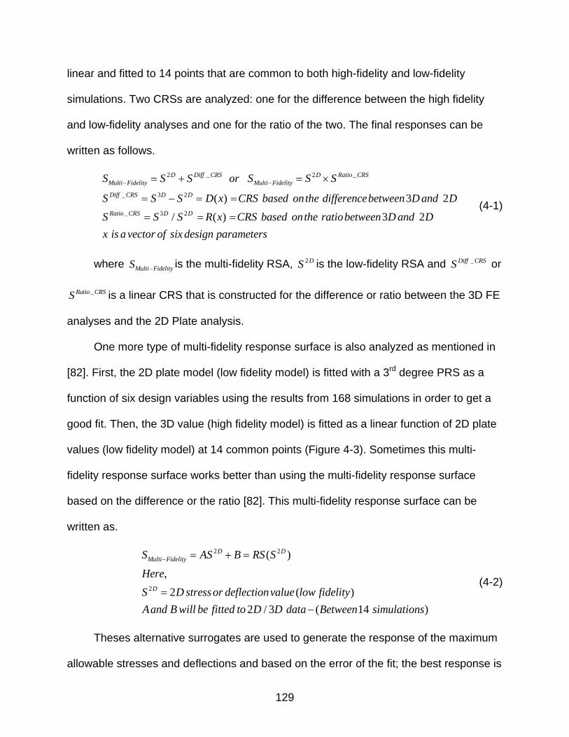
129
linear and fitted to 14 points that are common to both high-fidelity and low-fidelity
simulations. Two CRSs are analyzed: one for the difference between the high fidelity
and low-fidelity analyses and one for the ratio of the two. The final responses can be
written as follows.
2 _ 2 _
_ 3 2
_ 3 2
( ) 3 2
/ ( ) 3 2
D Diff CRS D Ratio CRS
Multi Fidelity Multi Fidelity
Diff CRS D D
Ratio CRS D D
S S S or S S S
S S S D x CRS based onthe differencebetween D and D
S S S R x CRS based onthe ratiobetween D and D
x is a vector of six design pa
rameters
(4-1)
where Multi FidelityS
is the multi-fidelity RSA, 2DS is the low-fidelity RSA and _Diff CRSS or
_Ratio CRSS is a linear CRS that is constructed for the difference or ratio between the 3D FE
analyses and the 2D Plate analysis.
One more type of multi-fidelity response surface is also analyzed as mentioned in
[82]. First, the 2D plate model (low fidelity model) is fitted with a 3rd degree PRS as a
function of six design variables using the results from 168 simulations in order to get a
good fit. Then, the 3D value (high fidelity model) is fitted as a linear function of 2D plate
values (low fidelity model) at 14 common points (Figure 4-3). Sometimes this multi-
fidelity response surface works better than using the multi-fidelity response surface
based on the difference or the ratio [82]. This multi-fidelity response surface can be
written as.
2 2
2
( )
,
2 ( )
2 / 3 ( 14 )
D D
Multi Fidelity
D
S AS B RS S
Here
S D stress or deflectionvalue low fidelity
Aand B will be fitted to D D data Between simulations
(4-2)
Theses alternative surrogates are used to generate the response of the maximum
allowable stresses and deflections and based on the error of the fit; the best response is
130
chosen for design optimization. As mentioned before, there are two important types of
loads that need to be considered in the design optimization of an ITPS. Both occur
during the reentry phase of the space vehicle. The two load cases are: (a) thermal load
due to severe temperature gradient across the thickness of the ITPS (b) aerodynamic
pressure load of 101 kPa acting on the top face sheet. Therefore, the response of the
stresses and deflections in the TFS, BFS and the web are generated for these loading
conditions as explained in the following sections.
Thermal Analysis
For the thermal loading case, initially the response surface for the maximum von
Mises stresses and the minimum buckling eigen value is generated as a function of six
design variables. However, later it was realized that for the stresses, this was not an
accurate way to represent the stress constraints with a single strength value, as the
strength value changes significantly with variation in the temperature. Also since there is
a temperature distribution across the thickness of the ITPS, the strength of the material
also changes. Therefore, instead of considering the maximum von Mises stress value,
the ratio of the maximum von Mises stress in each layer to the corresponding strength
value is considered and then the maximum ratio is used to fit with the design variables.
Temperature dependent strength values are obtained from [20] for both the Titanium
alloy and Beryllium alloy and is accurately represented by a cubic polynomial response
surface.
As mentioned before, 3D high-fidelity response and 2D low-fidelity response
surfaces were generated. The PRESS and standard error measure the error of the fit,
which in the case of the fit to the 3D results, is the only source of error. These errors are
also shown in Table 4-2. After generating the 3D and 2D response surfaces, the multi-
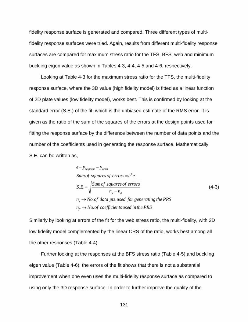
131
fidelity response surface is generated and compared. Three different types of multi-
fidelity response surfaces were tried. Again, results from different multi-fidelity response
surfaces are compared for maximum stress ratio for the TFS, BFS, web and minimum
buckling eigen value as shown in Tables 4-3, 4-4, 4-5 and 4-6, respectively.
Looking at Table 4-3 for the maximum stress ratio for the TFS, the multi-fidelity
response surface, where the 3D value (high fidelity model) is fitted as a linear function
of 2D plate values (low fidelity model), works best. This is confirmed by looking at the
standard error (S.E.) of the fit, which is the unbiased estimate of the RMS error. It is
given as the ratio of the sum of the squares of the errors at the design points used for
fitting the response surface by the difference between the number of data points and the
number of the coefficients used in generating the response surface. Mathematically,
S.E. can be written as,
. .
. .
.
response exact
T
y
y
e y y
Sumof squares of errors e e
Sumof squares of errorsS E
n n
n No of data pts used for generating the PRS
n No of coefficientsused in the PRS
(4-3)
Similarly by looking at errors of the fit for the web stress ratio, the multi-fidelity, with 2D
low fidelity model complemented by the linear CRS of the ratio, works best among all
the other responses (Table 4-4).
Further looking at the responses at the BFS stress ratio (Table 4-5) and buckling
eigen value (Table 4-6), the errors of the fit shows that there is not a substantial
improvement when one even uses the multi-fidelity response surface as compared to
using only the 3D response surface. In order to further improve the quality of the
132
response surface, a sensitivity analysis is performed [84] using the 3D response
surfaces. Sensitivity can be defined as a measure of the contribution of an independent
variable to the total variance of the dependent data. By doing this, the more important
design variables can be found, which can be used to regenerate the responses in order
to get a better fit for the same number of experiments. Now looking at the sensitivity bar
graph for BFS stress ratio (Figure 4-4), the more important design variables are the TFS
thickness tTF, BFS thickness tBF, and height of the sandwich panel d. For a quadratic
PRS based on three design variables, the number of coefficients is 10. Hence, in order
to generate the quadratic response surface for the 3D PRS and the CRS PRS, the
numbers of simulation results were increased from 14 to 20 3D simulations. Looking at
the errors of the fit from the Table 4-7 for the maximum stress ratio for the BFS, it can
be seen that the multi-fidelity CRS ratio works the best. Again, looking at the sensitivity
bar graph for buckling eigen value (Figure 4-5), the more important design variables are
the BFS thickness tBF, web thickness tW, and height of the sandwich panel d. Initially,
PRS was tried for the 3D response surface and the multi-fidelity response surface.
Since the PRS did not give a good fit, support vector regression (SVR) was tried.
Looking at the errors of the various fit from Table 4-8, the multi-fidelity, with 2D low
fidelity model complemented by the CRS of the ratio, works best among all the other
responses. The kernel function for both the 2D and CRS ratio that was used for
generating the multi-fidelity response is „Linear Spline‟ with - insensitive (Figure 4-2)
value for the 2D and CRS ratio as 0.0155 and 0.02, respectively. Now in order to
validate that various option of each responses selected based on the errors of the fit is
indeed the best option, it has been validated by calculating the errors at test points.
133
These test points were not used to fit the data and the errors at the test points also
confirms the choice as seen from the Tables 4-3, 4-4, 4-5 and 4-6.
Pressure Analysis
For the pressure loading case, the response surfaces for the maximum von Mises
stresses, maximum deflection and the minimum buckling eigen value are generated as
a function of six design variables. For the pressure case, only the 3D response surface
was generated. As compared to thermal load case, the stresses under the pressure
load were very small and much lesser than the yield strength values of the material
used. Therefore, the complex 2D and the multi-fidelity approach were not used to
further improve the accuracy of the response surface. The R2 and standard error
measure the error of the fit, which in the case of the fit to the 3D results, is the only
source of error. These errors are also shown in Table 4-9.
After generating these 3D response surfaces, a sensitivity analysis is done in
order to check if there is any further improvement in the quality of the 3D response
surfaces. The responses are regenerated using only the important design variables in
order to get a better fit for the same number of experiments. Finally, the results for
different 3D response surfaces are compared for the maximum von Mises stresses in
the TFS, BFS and web, maximum TFS deflection and minimum buckling eigen value as
shown in Tables 4-10, 4-11, 4-12, 4-13 and 4-14, respectively.
Now looking at the sensitivity bar graph for TFS maximum von Mises stress
(Figure 4-6), the more important design variables are the TFS thickness tTF, BFS
thickness tBF, height of the sandwich panel d and length of the panel, L. Now for these
four design variables, generating a quadratic PRS involves 15 coefficients. Hence, in
order to generate the quadratic response surface for the 3D PRS, the numbers of
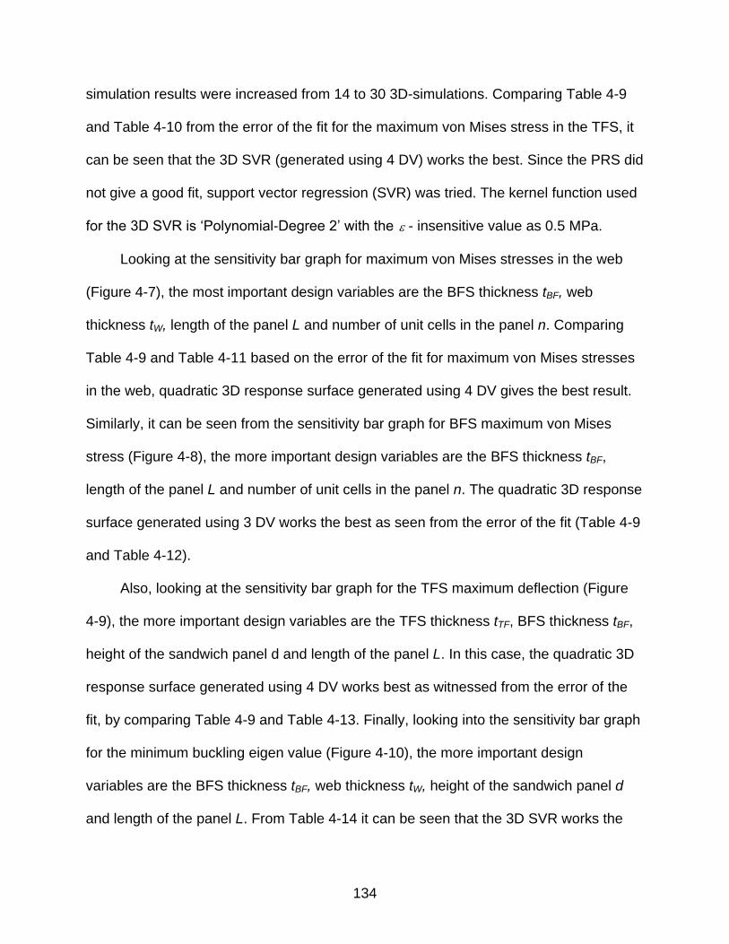
134
simulation results were increased from 14 to 30 3D-simulations. Comparing Table 4-9
and Table 4-10 from the error of the fit for the maximum von Mises stress in the TFS, it
can be seen that the 3D SVR (generated using 4 DV) works the best. Since the PRS did
not give a good fit, support vector regression (SVR) was tried. The kernel function used
for the 3D SVR is „Polynomial-Degree 2‟ with the - insensitive value as 0.5 MPa.
Looking at the sensitivity bar graph for maximum von Mises stresses in the web
(Figure 4-7), the most important design variables are the BFS thickness tBF, web
thickness tW, length of the panel L and number of unit cells in the panel n. Comparing
Table 4-9 and Table 4-11 based on the error of the fit for maximum von Mises stresses
in the web, quadratic 3D response surface generated using 4 DV gives the best result.
Similarly, it can be seen from the sensitivity bar graph for BFS maximum von Mises
stress (Figure 4-8), the more important design variables are the BFS thickness tBF,
length of the panel L and number of unit cells in the panel n. The quadratic 3D response
surface generated using 3 DV works the best as seen from the error of the fit (Table 4-9
and Table 4-12).
Also, looking at the sensitivity bar graph for the TFS maximum deflection (Figure
4-9), the more important design variables are the TFS thickness tTF, BFS thickness tBF,
height of the sandwich panel d and length of the panel L. In this case, the quadratic 3D
response surface generated using 4 DV works best as witnessed from the error of the
fit, by comparing Table 4-9 and Table 4-13. Finally, looking into the sensitivity bar graph
for the minimum buckling eigen value (Figure 4-10), the more important design
variables are the BFS thickness tBF, web thickness tW, height of the sandwich panel d
and length of the panel L. From Table 4-14 it can be seen that the 3D SVR works the
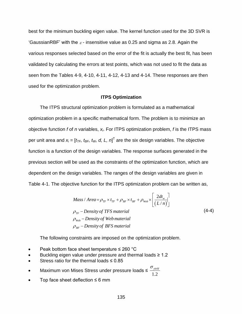
135
best for the minimum buckling eigen value. The kernel function used for the 3D SVR is
„GaussianRBF‟ with the - insensitive value as 0.25 and sigma as 2.8. Again the
various responses selected based on the error of the fit is actually the best fit, has been
validated by calculating the errors at test points, which was not used to fit the data as
seen from the Tables 4-9, 4-10, 4-11, 4-12, 4-13 and 4-14. These responses are then
used for the optimization problem.
ITPS Optimization
The ITPS structural optimization problem is formulated as a mathematical
optimization problem in a specific mathematical form. The problem is to minimize an
objective function f of n variables, xi. For ITPS optimization problem, f is the ITPS mass
per unit area and xi = [tTF, tBF, tW, d, L, n]T are the six design variables. The objective
function is a function of the design variables. The response surfaces generated in the
previous section will be used as the constraints of the optimization function, which are
dependent on the design variables. The ranges of the design variables are given in
Table 4-1. The objective function for the ITPS optimization problem can be written as,
2/
/
wTF TF BF BF Web
TF
Web
BF
dtMass Area t t
L n
Density of TFS material
Density of Webmaterial
Density of BFS material
(4-4)
The following constraints are imposed on the optimization problem.
Peak bottom face sheet temperature ≤ 260 °C
Buckling eigen value under pressure and thermal loads ≥ 1.2
Stress ratio for the thermal loads ≤ 0.85
Maximum von Mises Stress under pressure loads ≤ 1.2
yield
Top face sheet deflection ≤ 6 mm
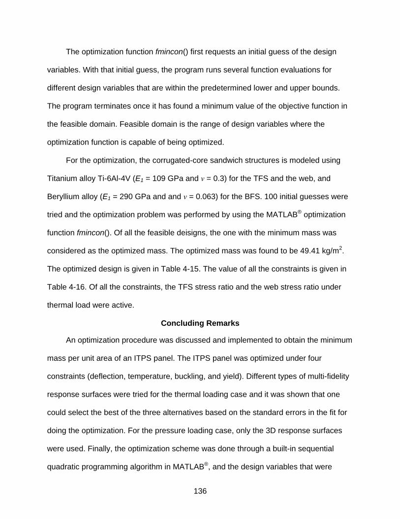
136
The optimization function fmincon() first requests an initial guess of the design
variables. With that initial guess, the program runs several function evaluations for
different design variables that are within the predetermined lower and upper bounds.
The program terminates once it has found a minimum value of the objective function in
the feasible domain. Feasible domain is the range of design variables where the
optimization function is capable of being optimized.
For the optimization, the corrugated-core sandwich structures is modeled using
Titanium alloy Ti-6Al-4V (E1 = 109 GPa and ν = 0.3) for the TFS and the web, and
Beryllium alloy (E1 = 290 GPa and and ν = 0.063) for the BFS. 100 initial guesses were
tried and the optimization problem was performed by using the MATLAB® optimization
function fmincon(). Of all the feasible deisigns, the one with the minimum mass was
considered as the optimized mass. The optimized mass was found to be 49.41 kg/m2.
The optimized design is given in Table 4-15. The value of all the constraints is given in
Table 4-16. Of all the constraints, the TFS stress ratio and the web stress ratio under
thermal load were active.
Concluding Remarks
An optimization procedure was discussed and implemented to obtain the minimum
mass per unit area of an ITPS panel. The ITPS panel was optimized under four
constraints (deflection, temperature, buckling, and yield). Different types of multi-fidelity
response surfaces were tried for the thermal loading case and it was shown that one
could select the best of the three alternatives based on the standard errors in the fit for
doing the optimization. For the pressure loading case, only the 3D response surfaces
were used. Finally, the optimization scheme was done through a built-in sequential
quadratic programming algorithm in MATLAB®, and the design variables that were

137
considered are ITPS width, thickness, number of unit cells, and thickness of each
component.
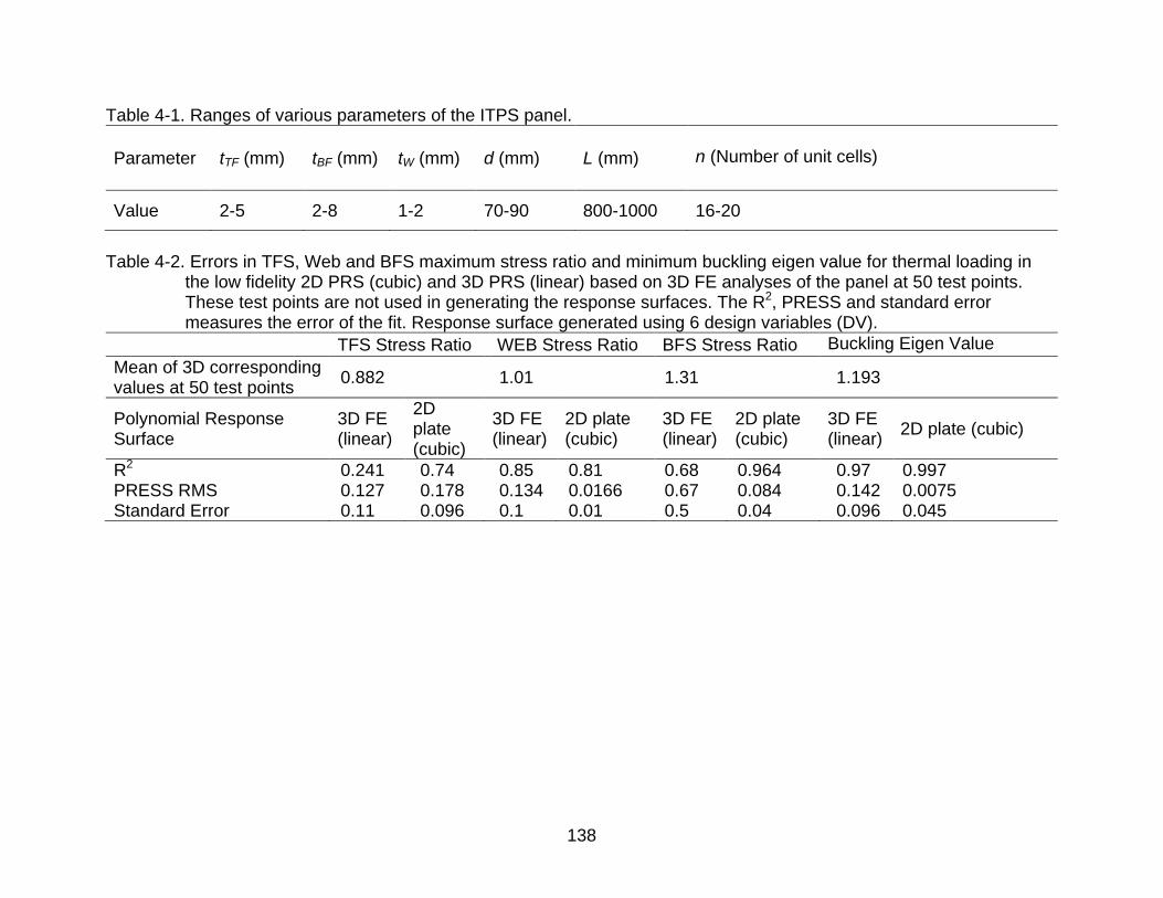
138
Table 4-1. Ranges of various parameters of the ITPS panel.
Parameter tTF (mm) tBF (mm) tW (mm) d (mm) L (mm)
n (Number of unit cells)
Value 2-5 2-8 1-2 70-90 800-1000 16-20
Table 4-2. Errors in TFS, Web and BFS maximum stress ratio and minimum buckling eigen value for thermal loading in
the low fidelity 2D PRS (cubic) and 3D PRS (linear) based on 3D FE analyses of the panel at 50 test points. These test points are not used in generating the response surfaces. The R2, PRESS and standard error measures the error of the fit. Response surface generated using 6 design variables (DV).
TFS Stress Ratio WEB Stress Ratio BFS Stress Ratio Buckling Eigen Value
Mean of 3D corresponding values at 50 test points
0.882 1.01 1.31 1.193
Polynomial Response Surface
3D FE (linear)
2D plate (cubic)
3D FE (linear)
2D plate (cubic)
3D FE (linear)
2D plate (cubic)
3D FE (linear)
2D plate (cubic)
R2 0.241 0.74 0.85 0.81 0.68 0.964 0.97 0.997 PRESS RMS 0.127 0.178 0.134 0.0166 0.67 0.084 0.142 0.0075 Standard Error 0.11 0.096 0.1 0.01 0.5 0.04 0.096 0.045
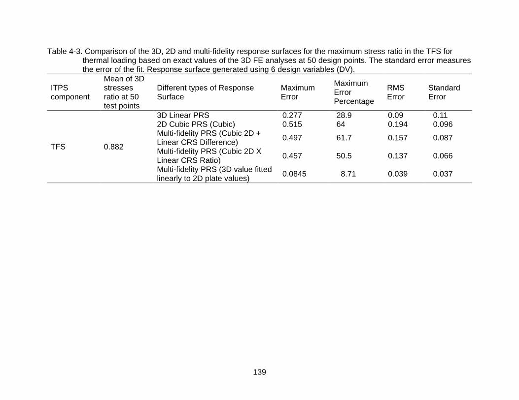
139
Table 4-3. Comparison of the 3D, 2D and multi-fidelity response surfaces for the maximum stress ratio in the TFS for thermal loading based on exact values of the 3D FE analyses at 50 design points. The standard error measures the error of the fit. Response surface generated using 6 design variables (DV).
ITPS component
Mean of 3D stresses ratio at 50 test points
Different types of Response Surface
Maximum Error
Maximum Error Percentage
RMS Error
Standard Error
TFS 0.882
3D Linear PRS 0.277 28.9 0.09 0.11 2D Cubic PRS (Cubic) 0.515 64 0.194 0.096 Multi-fidelity PRS (Cubic 2D + Linear CRS Difference)
0.497 61.7 0.157 0.087
Multi-fidelity PRS (Cubic 2D X Linear CRS Ratio)
0.457 50.5 0.137 0.066
Multi-fidelity PRS (3D value fitted linearly to 2D plate values)
0.0845 8.71 0.039 0.037
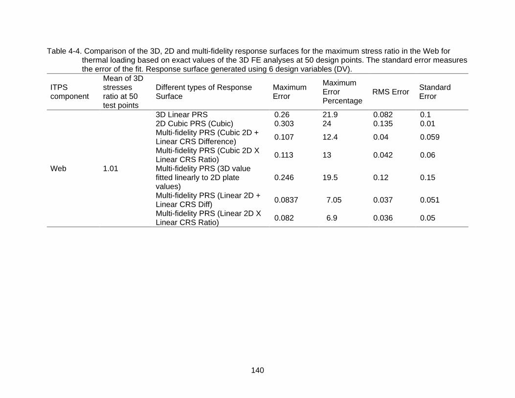
140
Table 4-4. Comparison of the 3D, 2D and multi-fidelity response surfaces for the maximum stress ratio in the Web for thermal loading based on exact values of the 3D FE analyses at 50 design points. The standard error measures the error of the fit. Response surface generated using 6 design variables (DV).
ITPS component
Mean of 3D stresses ratio at 50 test points
Different types of Response Surface
Maximum Error
Maximum Error Percentage
RMS Error Standard Error
Web 1.01
3D Linear PRS 0.26 21.9 0.082 0.1 2D Cubic PRS (Cubic) 0.303 24 0.135 0.01 Multi-fidelity PRS (Cubic 2D + Linear CRS Difference)
0.107 12.4 0.04 0.059
Multi-fidelity PRS (Cubic 2D X Linear CRS Ratio)
0.113 13 0.042 0.06
Multi-fidelity PRS (3D value fitted linearly to 2D plate values)
0.246 19.5 0.12 0.15
Multi-fidelity PRS (Linear 2D + Linear CRS Diff)
0.0837 7.05 0.037 0.051
Multi-fidelity PRS (Linear 2D X Linear CRS Ratio)
0.082 6.9 0.036 0.05
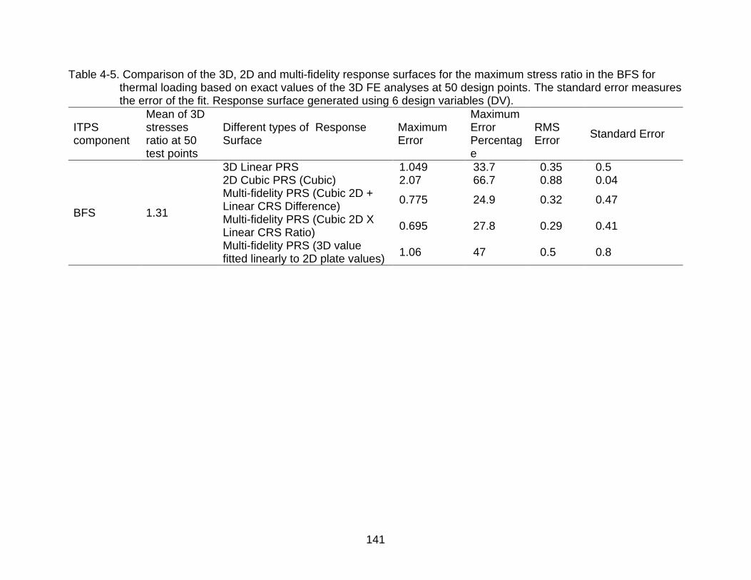
141
Table 4-5. Comparison of the 3D, 2D and multi-fidelity response surfaces for the maximum stress ratio in the BFS for thermal loading based on exact values of the 3D FE analyses at 50 design points. The standard error measures the error of the fit. Response surface generated using 6 design variables (DV).
ITPS component
Mean of 3D stresses ratio at 50 test points
Different types of Response Surface
Maximum Error
Maximum Error Percentage
RMS Error
Standard Error
BFS 1.31
3D Linear PRS 1.049 33.7 0.35 0.5 2D Cubic PRS (Cubic) 2.07 66.7 0.88 0.04 Multi-fidelity PRS (Cubic 2D + Linear CRS Difference)
0.775 24.9 0.32 0.47
Multi-fidelity PRS (Cubic 2D X Linear CRS Ratio)
0.695 27.8 0.29 0.41
Multi-fidelity PRS (3D value fitted linearly to 2D plate values)
1.06 47 0.5 0.8
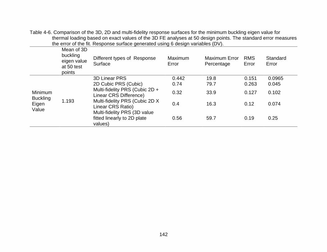
142
Table 4-6. Comparison of the 3D, 2D and multi-fidelity response surfaces for the minimum buckling eigen value for thermal loading based on exact values of the 3D FE analyses at 50 design points. The standard error measures the error of the fit. Response surface generated using 6 design variables (DV).
Mean of 3D buckling eigen value at 50 test points
Different types of Response Surface
Maximum Error
Maximum Error Percentage
RMS Error
Standard Error
Minimum Buckling Eigen Value
1.193
3D Linear PRS 0.442 19.8 0.151 0.0965 2D Cubic PRS (Cubic) 0.74 79.7 0.263 0.045 Multi-fidelity PRS (Cubic 2D + Linear CRS Difference)
0.32 33.9 0.127 0.102
Multi-fidelity PRS (Cubic 2D X Linear CRS Ratio)
0.4 16.3 0.12 0.074
Multi-fidelity PRS (3D value fitted linearly to 2D plate values)
0.56 59.7 0.19 0.25
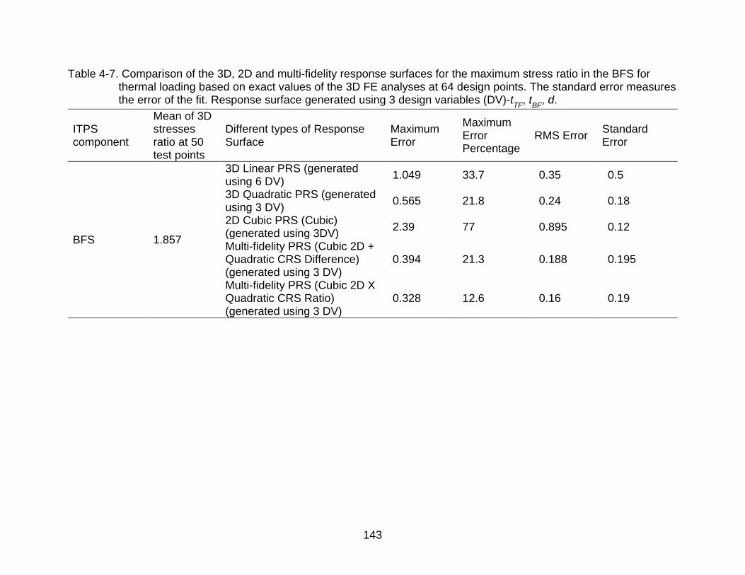
143
Table 4-7. Comparison of the 3D, 2D and multi-fidelity response surfaces for the maximum stress ratio in the BFS for thermal loading based on exact values of the 3D FE analyses at 64 design points. The standard error measures the error of the fit. Response surface generated using 3 design variables (DV)-t
TF, t
BF, d.
ITPS component
Mean of 3D stresses ratio at 50 test points
Different types of Response Surface
Maximum Error
Maximum Error Percentage
RMS Error Standard Error
BFS 1.857
3D Linear PRS (generated using 6 DV)
1.049 33.7 0.35 0.5
3D Quadratic PRS (generated using 3 DV)
0.565 21.8 0.24 0.18
2D Cubic PRS (Cubic) (generated using 3DV)
2.39 77 0.895 0.12
Multi-fidelity PRS (Cubic 2D + Quadratic CRS Difference) (generated using 3 DV)
0.394 21.3 0.188 0.195
Multi-fidelity PRS (Cubic 2D X Quadratic CRS Ratio) (generated using 3 DV)
0.328 12.6 0.16 0.19
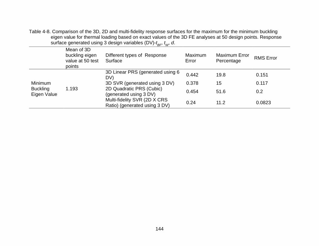
144
Table 4-8. Comparison of the 3D, 2D and multi-fidelity response surfaces for the maximum for the minimum buckling eigen value for thermal loading based on exact values of the 3D FE analyses at 50 design points. Response surface generated using 3 design variables (DV)-t
BF, t
W, d.
Mean of 3D buckling eigen value at 50 test points
Different types of Response Surface
Maximum Error
Maximum Error Percentage
RMS Error
Minimum Buckling Eigen Value
1.193
3D Linear PRS (generated using 6 DV)
0.442 19.8 0.151
3D SVR (generated using 3 DV) 0.378 15 0.117 2D Quadratic PRS (Cubic) (generated using 3 DV)
0.454 51.6 0.2
Multi-fidelity SVR (2D X CRS Ratio) (generated using 3 DV)
0.24 11.2 0.0823
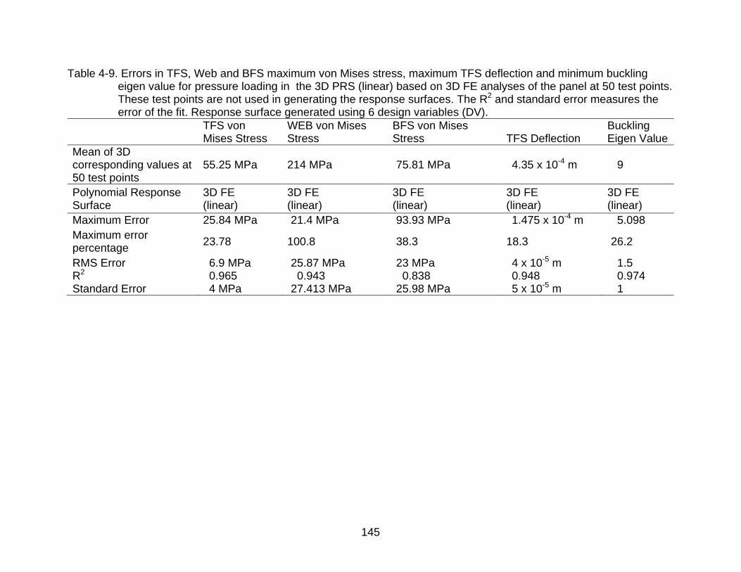
145
Table 4-9. Errors in TFS, Web and BFS maximum von Mises stress, maximum TFS deflection and minimum buckling eigen value for pressure loading in the 3D PRS (linear) based on 3D FE analyses of the panel at 50 test points. These test points are not used in generating the response surfaces. The R2 and standard error measures the error of the fit. Response surface generated using 6 design variables (DV).
TFS von Mises Stress
WEB von Mises Stress
BFS von Mises Stress
TFS Deflection
Buckling Eigen Value
Mean of 3D corresponding values at 50 test points
55.25 MPa 214 MPa 75.81 MPa 4.35 x 10⁻⁴ m
9
Polynomial Response Surface
3D FE (linear)
3D FE (linear)
3D FE (linear)
3D FE (linear)
3D FE (linear)
Maximum Error 25.84 MPa 21.4 MPa 93.93 MPa 1.475 x 10⁻⁴ m 5.098
Maximum error percentage
23.78 100.8 38.3 18.3 26.2
RMS Error 6.9 MPa 25.87 MPa 23 MPa 4 x 10⁻⁵ m 1.5 R2 0.965 0.943 0.838 0.948 0.974 Standard Error 4 MPa 27.413 MPa 25.98 MPa 5 x 10⁻⁵ m 1
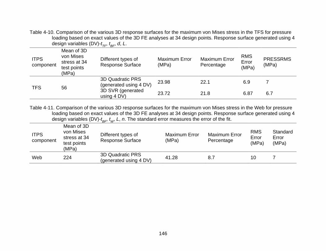
146
Table 4-10. Comparison of the various 3D response surfaces for the maximum von Mises stress in the TFS for pressure loading based on exact values of the 3D FE analyses at 34 design points. Response surface generated using 4 design variables (DV)-t
TF, t
BF, d, L.
ITPS component
Mean of 3D von Mises stress at 34 test points (MPa)
Different types of Response Surface
Maximum Error (MPa)
Maximum Error Percentage
RMS Error (MPa)
PRESSRMS (MPa)
TFS 56
3D Quadratic PRS (generated using 4 DV)
23.98 22.1 6.9 7
3D SVR (generated using 4 DV)
23.72 21.8 6.87 6.7
Table 4-11. Comparison of the various 3D response surfaces for the maximum von Mises stress in the Web for pressure
loading based on exact values of the 3D FE analyses at 34 design points. Response surface generated using 4 design variables (DV)-t
BF, t
W, L, n. The standard error measures the error of the fit.
ITPS component
Mean of 3D von Mises stress at 34 test points (MPa)
Different types of Response Surface
Maximum Error (MPa)
Maximum Error Percentage
RMS Error (MPa)
Standard Error (MPa)
Web 224 3D Quadratic PRS (generated using 4 DV)
41.28 8.7 10 7
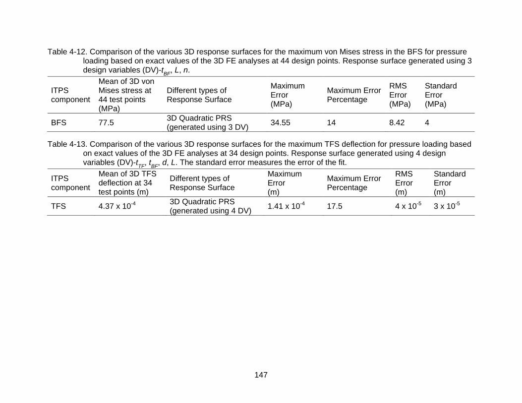
147
Table 4-12. Comparison of the various 3D response surfaces for the maximum von Mises stress in the BFS for pressure loading based on exact values of the 3D FE analyses at 44 design points. Response surface generated using 3 design variables (DV)-t
BF, L, n.
ITPS component
Mean of 3D von Mises stress at 44 test points (MPa)
Different types of Response Surface
Maximum Error (MPa)
Maximum Error Percentage
RMS Error (MPa)
Standard Error (MPa)
BFS 77.5 3D Quadratic PRS (generated using 3 DV)
34.55 14 8.42 4
Table 4-13. Comparison of the various 3D response surfaces for the maximum TFS deflection for pressure loading based on exact values of the 3D FE analyses at 34 design points. Response surface generated using 4 design variables (DV)-t
TF, t
BF, d, L. The standard error measures the error of the fit.
ITPS component
Mean of 3D TFS deflection at 34 test points (m)
Different types of Response Surface
Maximum Error (m)
Maximum Error Percentage
RMS Error (m)
Standard Error (m)
TFS 4.37 x 10⁻⁴ 3D Quadratic PRS (generated using 4 DV)
1.41 x 10⁻⁴ 17.5 4 x 10⁻⁵ 3 x 10⁻⁵
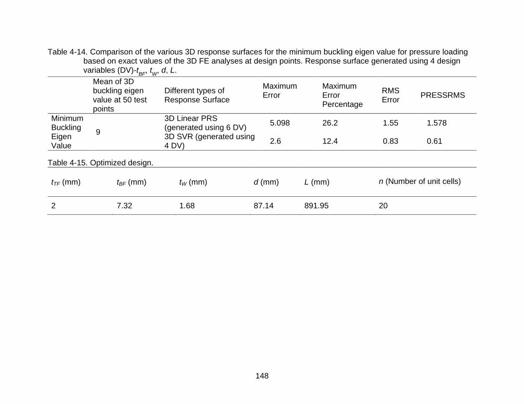
148
Table 4-14. Comparison of the various 3D response surfaces for the minimum buckling eigen value for pressure loading based on exact values of the 3D FE analyses at design points. Response surface generated using 4 design variables (DV)-t
BF, t
W, d, L.
Mean of 3D buckling eigen value at 50 test points
Different types of Response Surface
Maximum Error
Maximum Error Percentage
RMS Error
PRESSRMS
Minimum Buckling Eigen Value
9
3D Linear PRS (generated using 6 DV)
5.098 26.2 1.55 1.578
3D SVR (generated using 4 DV)
2.6 12.4 0.83 0.61
Table 4-15. Optimized design.
tTF (mm) tBF (mm) tW (mm) d (mm) L (mm)
n (Number of unit cells)
2 7.32 1.68 87.14 891.95 20
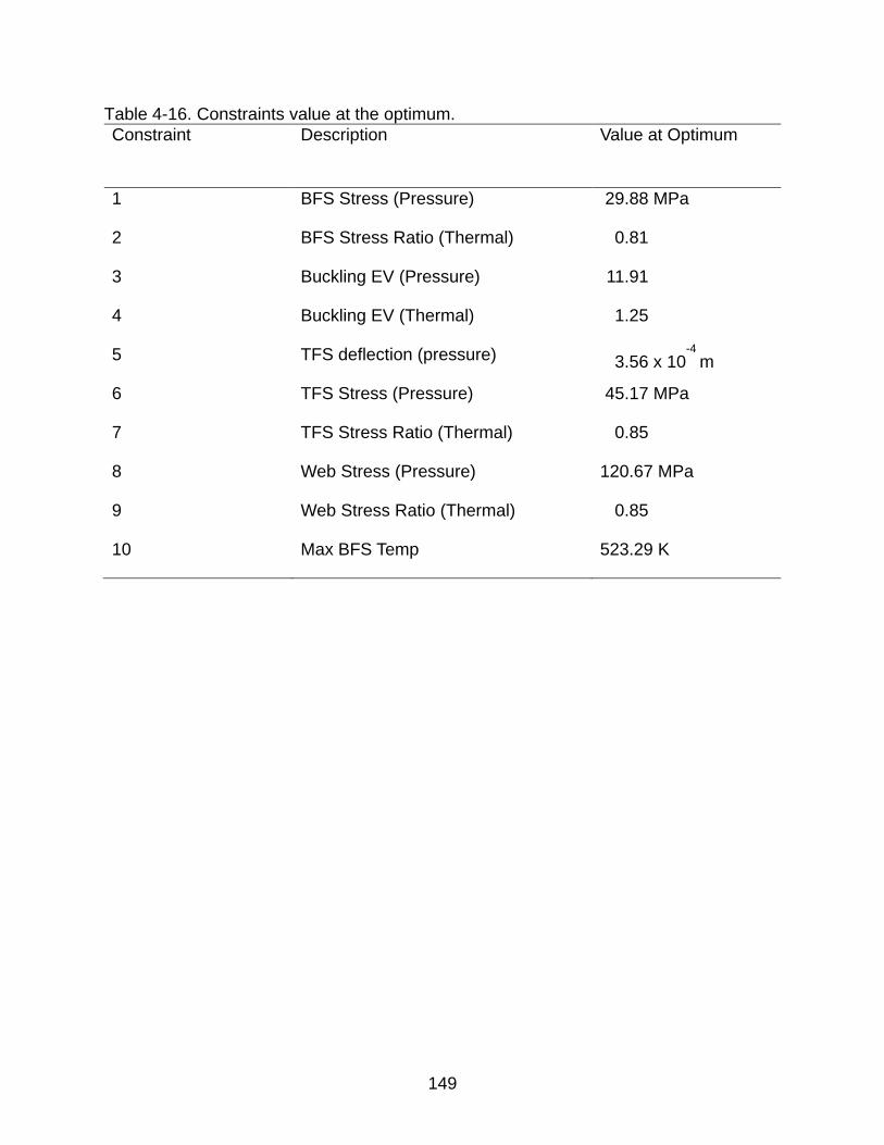
149
Table 4-16. Constraints value at the optimum.
Constraint Description Value at Optimum
1 BFS Stress (Pressure) 29.88 MPa
2 BFS Stress Ratio (Thermal) 0.81
3 Buckling EV (Pressure) 11.91
4 Buckling EV (Thermal) 1.25
5 TFS deflection (pressure) 3.56 x 10⁻⁴
m
6 TFS Stress (Pressure) 45.17 MPa
7 TFS Stress Ratio (Thermal) 0.85
8 Web Stress (Pressure) 120.67 MPa
9 Web Stress Ratio (Thermal) 0.85
10 Max BFS Temp 523.29 K
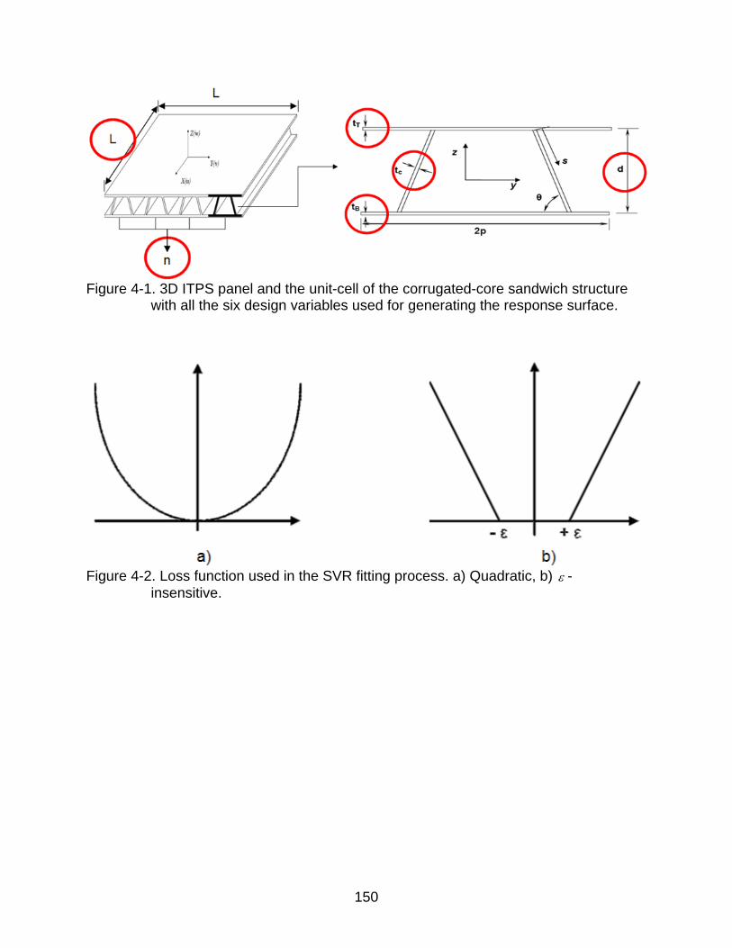
150
Figure 4-1. 3D ITPS panel and the unit-cell of the corrugated-core sandwich structure
with all the six design variables used for generating the response surface.
Figure 4-2. Loss function used in the SVR fitting process. a) Quadratic, b) -
insensitive.
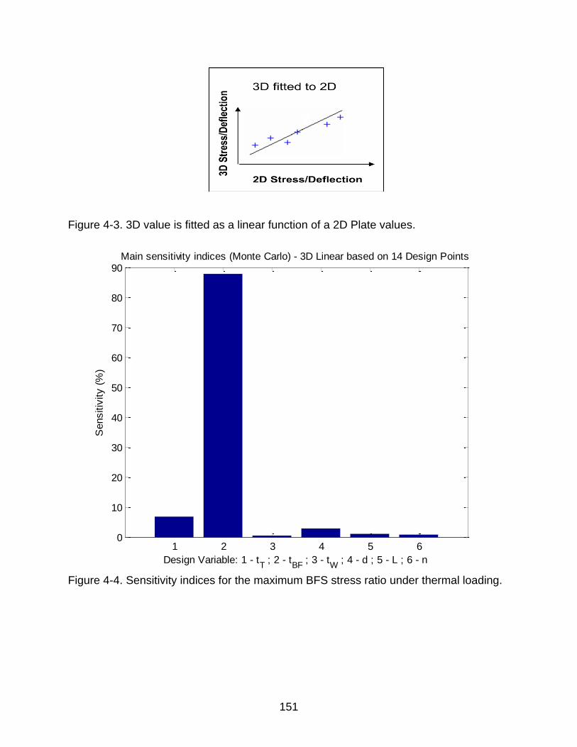
151
Figure 4-3. 3D value is fitted as a linear function of a 2D Plate values.
Figure 4-4. Sensitivity indices for the maximum BFS stress ratio under thermal loading.
1 2 3 4 5 60
10
20
30
40
50
60
70
80
90
Design Variable: 1 - tT ; 2 - t
BF ; 3 - t
W ; 4 - d ; 5 - L ; 6 - n
Sensitiv
ity (
%)
Main sensitivity indices (Monte Carlo) - 3D Linear based on 14 Design Points
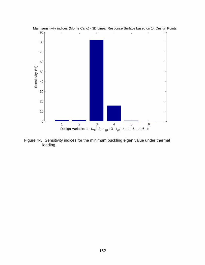
152
Figure 4-5. Sensitivity indices for the minimum buckling eigen value under thermal loading.
1 2 3 4 5 60
10
20
30
40
50
60
70
80
90Main sensitivity indices (Monte Carlo) - 3D Linear Response Surface based on 14 Design Points
Design Variable: 1 - tTF
; 2 - tBF
; 3 - tW
; 4 - d ; 5 - L ; 6 - n
Sensitiv
ity (
%)
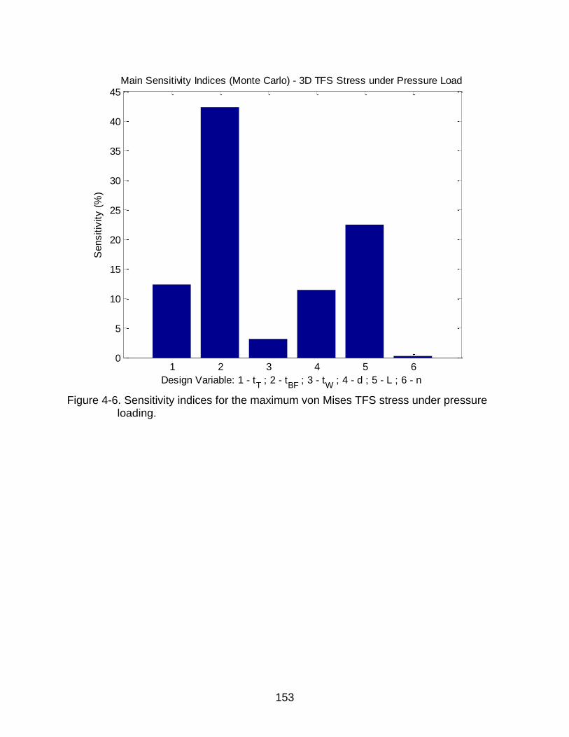
153
Figure 4-6. Sensitivity indices for the maximum von Mises TFS stress under pressure
loading.
1 2 3 4 5 60
5
10
15
20
25
30
35
40
45Main Sensitivity Indices (Monte Carlo) - 3D TFS Stress under Pressure Load
Design Variable: 1 - tT ; 2 - t
BF ; 3 - t
W ; 4 - d ; 5 - L ; 6 - n
Sensitiv
ity (
%)
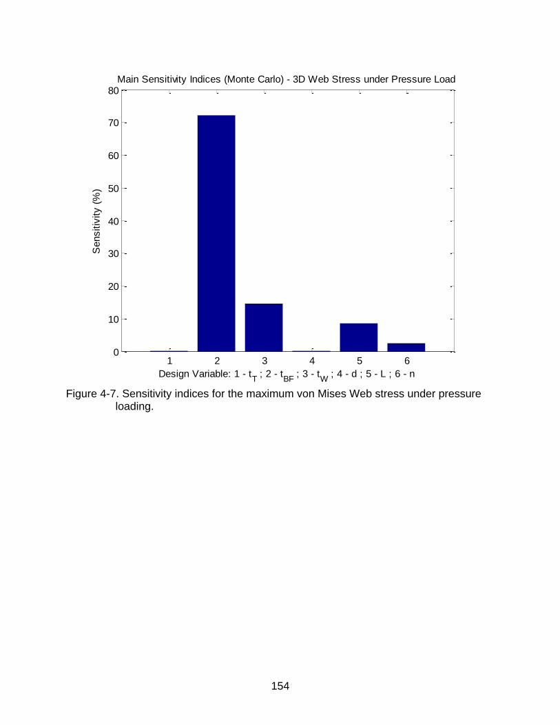
154
Figure 4-7. Sensitivity indices for the maximum von Mises Web stress under pressure
loading.
1 2 3 4 5 60
10
20
30
40
50
60
70
80
Design Variable: 1 - tT ; 2 - t
BF ; 3 - t
W ; 4 - d ; 5 - L ; 6 - n
Sensitiv
ity (
%)
Main Sensitivity Indices (Monte Carlo) - 3D Web Stress under Pressure Load
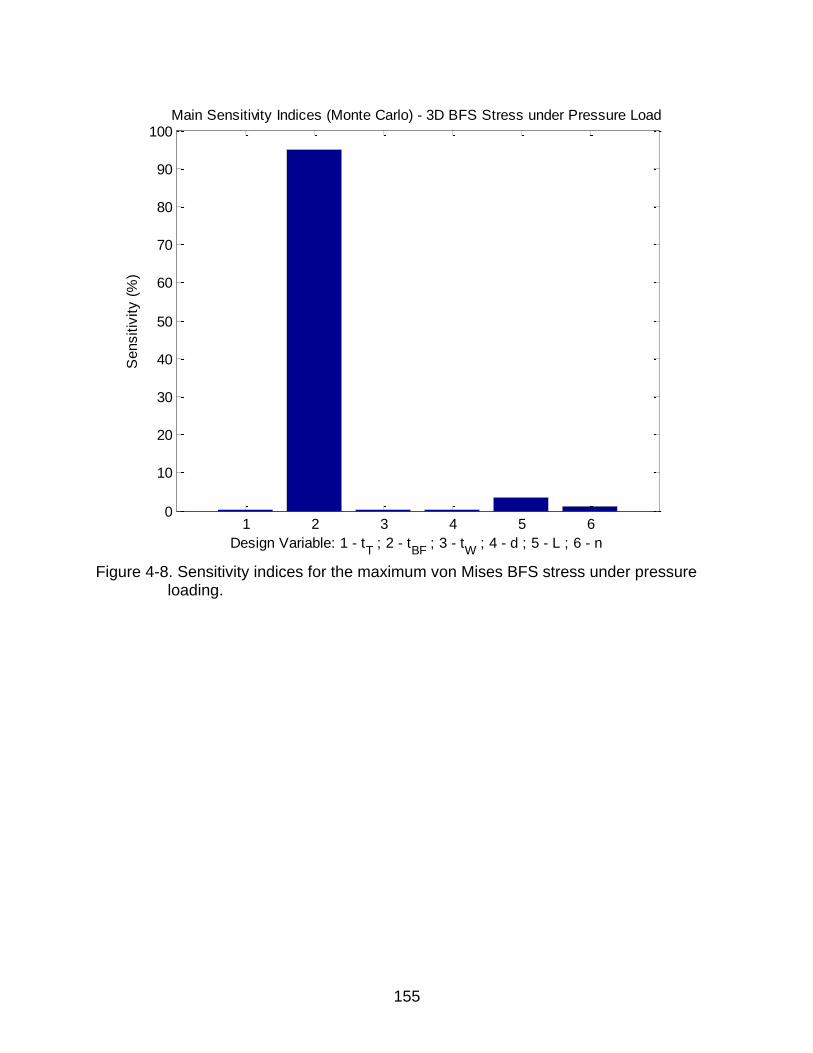
155
Figure 4-8. Sensitivity indices for the maximum von Mises BFS stress under pressure
loading.
1 2 3 4 5 60
10
20
30
40
50
60
70
80
90
100
Design Variable: 1 - tT ; 2 - t
BF ; 3 - t
W ; 4 - d ; 5 - L ; 6 - n
Sensitiv
ity (
%)
Main Sensitivity Indices (Monte Carlo) - 3D BFS Stress under Pressure Load
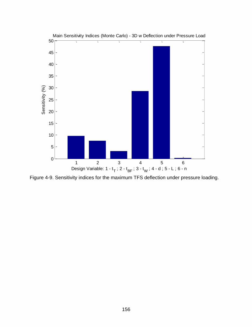
156
Figure 4-9. Sensitivity indices for the maximum TFS deflection under pressure loading.
1 2 3 4 5 60
5
10
15
20
25
30
35
40
45
50
Design Variable: 1 - tT ; 2 - t
BF ; 3 - t
W ; 4 - d ; 5 - L ; 6 - n
Sensitiv
ity (
%)
Main Sensitivity Indices (Monte Carlo) - 3D w Deflection under Pressure Load
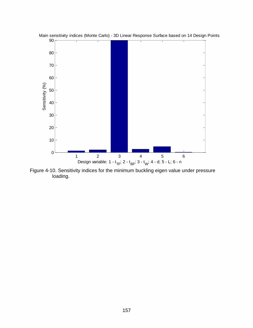
157
Figure 4-10. Sensitivity indices for the minimum buckling eigen value under pressure
loading.
1 2 3 4 5 60
10
20
30
40
50
60
70
80
90Main sensitivity indices (Monte Carlo) - 3D Linear Response Surface based on 14 Design Points
Design variable: 1 - tTF
; 2 - tBF
; 3 - tW
; 4 - d; 5 - L; 6 - n
Sensitiv
ity (
%)
158
CHAPTER 5 CONCLUSIONS
Summary
A brief overview of this research and findings are presented in this chapter. The
summary of the studies is mentioned with appropriate conclusions. Finally,
recommendations for further studies are presented. For any hypersonic re-entry vehicle,
thermal protection system (TPS) is one of the most critical structures. It protects the
vehicle from extreme re-entry temperatures. Future vehicles will require an efficient,
reusable, and advanced TPS technology that will provide the hypersonic vehicle with
the necessary protection from the extreme reentry environments as well as the cost and
maintenance is low. Chapter 1 discusses various prerequisites of the TPS and the
approaches which have been undertaken in the past. A variety of TPS concepts have
been reviewed and summarized. One such concept is the ITPS, which is the subject of
this dissertation. Knowing the underlying challenges of this ITPS development, the
specific objectives and purpose of the dissertation were laid out, which was to develop
FE based micro-mechanics methods and reverse homogenization method to predict the
behavior of any sandwich structure. This 2D FE based method has some limitation and
hence the accuracy of the method was improved further using the multi-fidelity
approach.
Chapter 2 contains the FE based homogenization procedure that is implemented
to determine the equivalent stiffness of the ITPS. This includes the extensional,
bending, coupling and shear stiffnesses of the sandwich structure. The result of different
stiffnesses is validated by comparing the maximum deflection under a transverse
pressure load between the 2D homogenized model and the 3D ITPS panel.
159
Chapter 3 discusses the detailed FE based reverse homogenization procedure to
predict the out of plane displacements and von Mises stresses under thermal and
pressure load from the 2D plate model. However, the plate model cannot capture the
local stresses and deflection in the TFS due to the transverse pressure load acting on it.
Therefore, a unit cell analysis approach is done in order to capture the local effects of
the pressure. Also, using the method of sub structuring, a unit cell buckling eigen value
analysis is done and compared with the corresponding 3D buckling eigen value
analysis.
Chapter 4 describes the various types of multi-fidelity approaches undertaken to
improve the accuracy of the 2D method. It was also seen that one could select the best
of the various alternative response surfaces, just based on the standard errors in the fit.
Using these response surfaces, the ITPS is optimized for minimum mass design. The
optimum design variables are obtained by minimizing the ITPS mass by satisfying all
the thermal protection systems requirements and limitation in the form of mathematical
constraints.
Concluding Remarks
A number of conclusions were explained at the end of each chapter. Some
general conclusions drawn from this research work are listed below.
The FE based homogenization and reverse homogenization is very robust and could be performed with any commercially available FE program. One can choose any material and dimension to implement on any sandwich structure (e.g., Z-cores, C-cores, and truss cores) and still be able to predict an accurate stiffness of the given structure.
Generally, the transverse shear stiffness is constant for a given cross-section. Unique transverse shear stiffness could not be found. Instead if one wants to select constant transverse shear stiffness, the best one will depend on the number of unit cells.
160
Difference between maximum deflection prediction from the 3D and 2D was less than 6%, indicating that the transverse shear stiffness prediction A44 and A55 is accurate.
2D approach can only work for L/h ratio greater than 8. Shorter L/h ratio could not effectively predict the stiffnesses as the boundary effects comes into play.
For a given transverse pressure load, maximum deflection occurs for rectangular webs whereas minimum deflection occurs for triangular web configuration.
Prediction of the buckling eigen value by using the method of sub structuring shows approximately 6-10% difference from the 3D buckling analysis under thermal loads.
The low fidelity 2D finite element model is fitted with a high quality surrogate, which is corrected by the use of a small number of high fidelity 3D finite element analyses. By doing this multi-fidelity approach, one can substantially improve the accuracy of the fit without doing large number of 3D finite element analysis.
One can choose the best correction model based on the data without the test points, and the test points also confirmed the choice.
Recommendations
Now that a general framework for FE based homogenization and reverse
homogenization procedure has been established with this research work, new structure
geometries can be explored. For the corrugated core design, buckling of the edges is
one of the major factors influencing the design. For example, buckling of the web-edges
close to the panel edges under thermal load is one of the first buckling modes. By
tactically placing stiffeners in the webs and face sheets, such buckling modes can be
prevented. Stiffeners do not add to the weight or heat conduction path of the ITPS
significantly, while drastically improving the buckling resistance of the structure.
Therefore, this line of design enhancement has a possibility for reducing the ITPS
weight significantly.
Another thing which was done for this research was that the unit cells were of
equal lengths. Instead unit cells of different length could be tried. Also there could be
161
large number of webs near the boundaries as most of the design drivers are near the
boundaries. One can also use thicker webs near the boundaries and thinner webs at the
center as they do not have high stresses near the center. Plane loads were not tried in
this research. Adding in plane loads could make the design even heavier.
We also found that the transverse shear stiffness for a corrugated core structure is
very high in one direction (along x) as compared to the other direction (along y). This is
a very unbalanced structure. One suggestion is that we can use corrugations in both the
directions (Figure 5-1). This way the shear stiffness can be equally distributed.
Three different types of correction approaches have been discussed in Chapter 4.
There is another type of correction technique that can be applied for the multi-fidelity
approach. This technique is called as space mapping. Suppose we have two design
variables, we can generate a linear response surface based on these two design
variables. We need to find the values of α, β, and γ, such that for that corresponding
value, my 2D response surface will be closer to the 3D values. This is different type of
multi-fidelity response surface and it is also represented in Equation 5-1 below.
3 2
1 2 1 2( , ) ( )D DS x x S x x (5-1)
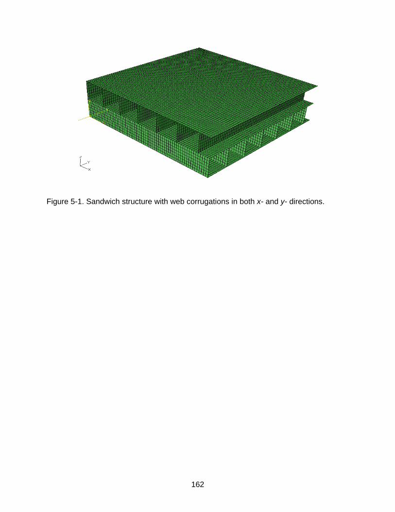
162
Figure 5-1. Sandwich structure with web corrugations in both x- and y- directions.
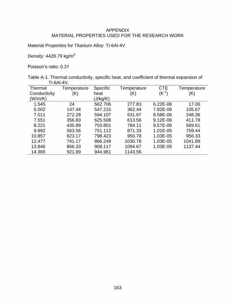
163
APPENDIX MATERIAL PROPERTIES USED FOR THE RESEARCH WORK
Material Properties for Titanium Alloy: Ti-6Al-4V
Density: 4428.79 kg/m3
Poisson‟s ratio: 0.31
Table A-1. Thermal conductivity, specific heat, and coefficient of thermal expansion of Ti-6Al-4V.
Thermal Conductivity (W/m/K)
Temperature (K)
Specific heat (J/kg/K)
Temperature (K)
CTE (K-1)
Temperature (K)
1.545 24 562.706 277.83 6.22E-06 17.06 5.002 147.44 547.215 362.44 7.82E-06 105.67 7.011 272.28 594.107 531.67 8.58E-06 248.36 7.551 356.83 625.508 613.56 9.12E-06 411.78 8.221 435.89 703.801 784.11 9.57E-06 569.61 9.992 563.56 751.112 871.33 1.01E-05 759.44
10.857 623.17 798.423 950.78 1.03E-05 956.33 12.477 741.17 866.249 1030.78 1.03E-05 1041.89 13.846 866.33 908.117 1094.67 1.03E-05 1137.44 14.365 921.89 944.961 1143.56
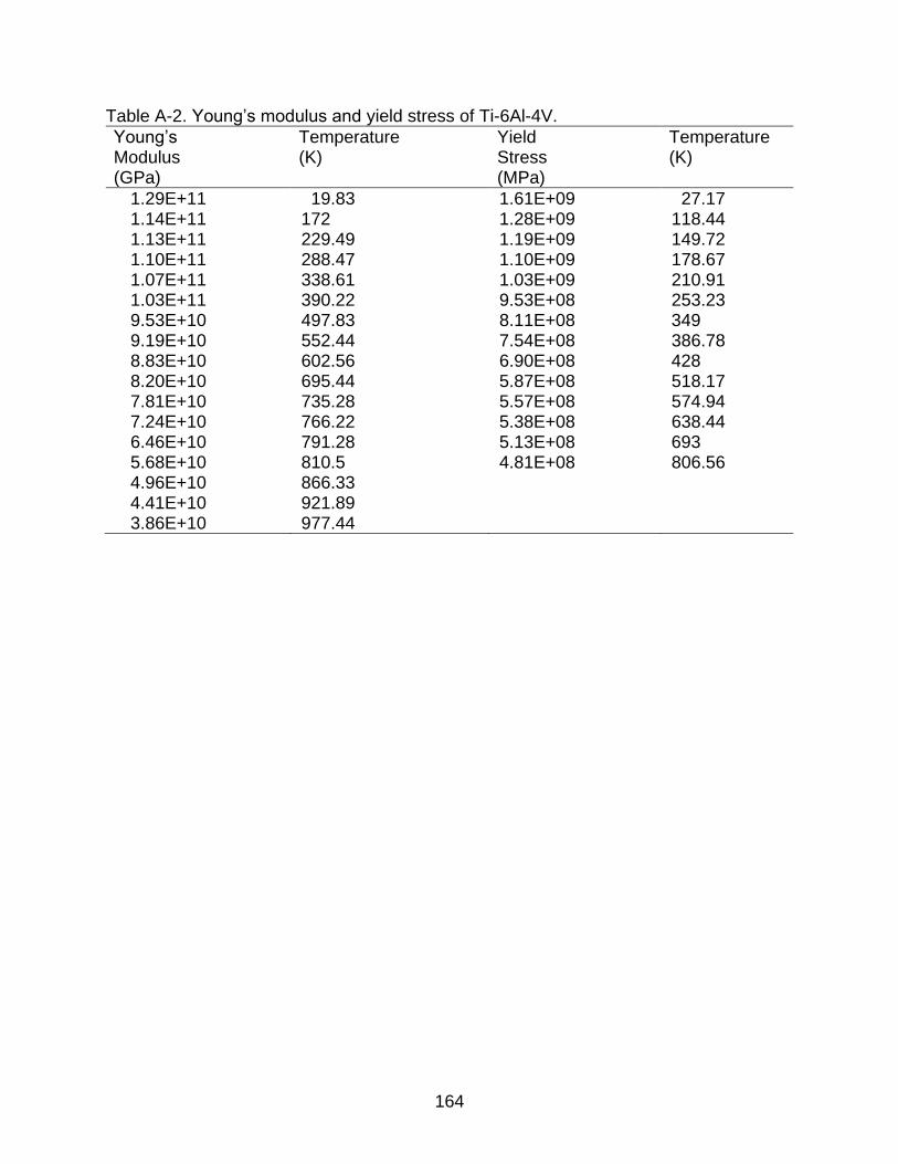
164
Table A-2. Young‟s modulus and yield stress of Ti-6Al-4V.
Young‟s Modulus (GPa)
Temperature (K)
Yield Stress (MPa)
Temperature (K)
1.29E+11 19.83 1.61E+09 27.17 1.14E+11 172 1.28E+09 118.44 1.13E+11 229.49 1.19E+09 149.72 1.10E+11 288.47 1.10E+09 178.67 1.07E+11 338.61 1.03E+09 210.91 1.03E+11 390.22 9.53E+08 253.23 9.53E+10 497.83 8.11E+08 349 9.19E+10 552.44 7.54E+08 386.78 8.83E+10 602.56 6.90E+08 428 8.20E+10 695.44 5.87E+08 518.17 7.81E+10 735.28 5.57E+08 574.94 7.24E+10 766.22 5.38E+08 638.44 6.46E+10 791.28 5.13E+08 693 5.68E+10 810.5 4.81E+08 806.56 4.96E+10 866.33 4.41E+10 921.89 3.86E+10 977.44
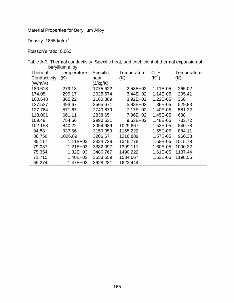
165
Material Properties for Beryllium Alloy
Density: 1855 kg/m3
Poisson‟s ratio: 0.063
Table A-3. Thermal conductivity, Specific heat, and coefficient of thermal expansion of beryllium alloy.
Thermal Conductivity (W/m/K)
Temperature (K)
Specific heat (J/kg/K)
Temperature (K)
CTE (K-1)
Temperature (K)
180.618 279.18 1775.622 2.58E+02 1.11E-05 265.02 174.05 299.17 2025.574 3.44E+02 1.14E-05 295.41 160.648 365.22 2160.389 3.92E+02 1.22E-05 366 137.527 493.67 2565.671 5.83E+02 1.36E-05 529.83 127.764 571.67 2740.679 7.17E+02 1.40E-05 581.22 118.001 661.11 2838.65 7.96E+02 1.45E-05 688 109.48 754.56 2990.631 9.53E+02 1.48E-05 733.72 102.158 840.22 3054.689 1029.667 1.53E-05 840.78 94.88 933.56 3159.359 1165.222 1.55E-05 884.11 88.756 1026.89 3206.67 1216.889 1.57E-05 966.33 85.117 1.11E+03 3324.738 1345.778 1.58E-05 1015.78 79.037 1.21E+03 3382.097 1399.111 1.60E-05 1090.22 75.354 1.32E+03 3486.767 1490.222 1.61E-05 1137.44 71.715 1.40E+03 3533.659 1534.667 1.63E-05 1198.56 69.274 1.47E+03 3628.281 1622.444
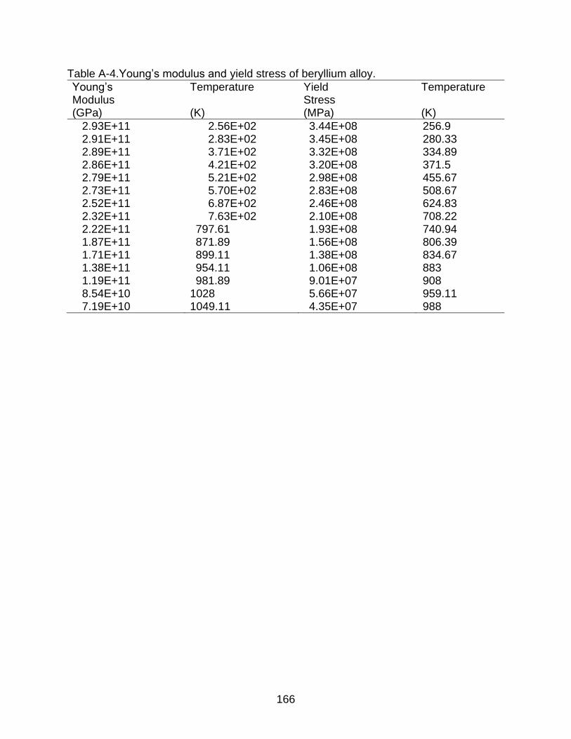
166
Table A-4.Young‟s modulus and yield stress of beryllium alloy.
Young‟s Modulus (GPa)
Temperature (K)
Yield Stress (MPa)
Temperature (K)
2.93E+11 2.56E+02 3.44E+08 256.9 2.91E+11 2.83E+02 3.45E+08 280.33 2.89E+11 3.71E+02 3.32E+08 334.89 2.86E+11 4.21E+02 3.20E+08 371.5 2.79E+11 5.21E+02 2.98E+08 455.67 2.73E+11 5.70E+02 2.83E+08 508.67 2.52E+11 6.87E+02 2.46E+08 624.83 2.32E+11 7.63E+02 2.10E+08 708.22 2.22E+11 797.61 1.93E+08 740.94 1.87E+11 871.89 1.56E+08 806.39 1.71E+11 899.11 1.38E+08 834.67 1.38E+11 954.11 1.06E+08 883 1.19E+11 981.89 9.01E+07 908 8.54E+10 1028 5.66E+07 959.11 7.19E+10 1049.11 4.35E+07 988
167
LIST OF REFERENCES
[1] Hunt, J. L., Lockwood, M. K., Petley, D. H., & Pegg, R. J. (1997, January). Hypersonic Airbreathing Vehicles Visions and Enhancing Technologies. Proceedings of the Space Technology and Applications International Forum, Albuquerque, NM, 387, 12851296.
[2] Blosser, M. L. (1996). Development of metallic thermal protection systems for the reusable launch vehicle. NASA TM110296.
[3] Christiansen, E. L., & Friesen, L. (1997). Penetration for thermal protection materials. International Journal of Impact Engineering, 20, 153164.
[4] Behrens, B., and Müller, M. (2004). Technologies for thermal protection systems applied on reusable launcher. Acta Astronautica, 55(39), 529536.
[5] Bohon, H. L., Shideler, J. L., & Rummler, D. R. (1977). Radiative metallic thermal protection systems: a status report. Journal of Spacecraft, 14(10), 626631.
[6] Bekey, I., Powell, R., Austin, R., “NASA Studies Access to Space,” Aerospace America, Vol. 32, No. 5, May 1994, pp. 38–43.
[7] Futron Corporation, “Space Transportation Costs: Trends in Price Per to Orbit 1990 – 2000,” Bethesda, MD: Author.
[8] Blosser, M. L., Chen, R. R., Schmidt, J. T., Dorsey, J. T., Poteet, C. C., Bird, R. K., & Wurster, K. E. (2004). Development of advanced thermal protection system prototype hardware. Journal of Spacecraft and Rockets, 41(2), 183194.
[9] Blosser, M. L., “Advanced Metallic Thermal Protection Systems for Reusable Launch Vehicles,” Ph.D. Dissertation, University of Virginia, May 2000.
[10] Dorsey, J. T., Poteet, C. C., Wurster, K. E., and Chen, R. R., “Metallic Thermal Protection System Requirements, Environments, and Integrated Concepts,” Journal of Spacecraft and Rockets, Vol. 41, No. 2, Mar–Apr 2004, pp. 162–172.
[11] Erb, R. B., Greenshields, D. H., Chauvin, L. T., Pavlosky, J. E., and Statham, C. L, “Apollo Thermal-Protection System Development,” Journal of Spacecraft (and Rockets), Vol. 7, No. 6, June 1970, pp. 727–734.
[12] Lee, G., “Ablation Effects on Apollo Afterbody Heat Transfer,” AIAA Journal, Vol. 7, No. 8, 1969, pp. 1616–1618.
[13] Braun, R. D., Powell, R. W., Evans Lyne, J., “Earth Aerobraking Strategies for Manned Return from Mars,” Journal of Spacecraft and Rockets, Vol. 29, No. 3, May–June 1992, pp. 297–304.
168
[14] Williams, S. D., Curry, D. M., Bouslog, S. A., Rochelle, W. C., “Thermal Protection System-Design Studies for Lunar Crew Module,” Journal of Spacecraft and Rockets, Vol. 32, No. 3, May–Jun 1995, pp. 456–462.
[15] Bartlett, E. P., Anderson, L. W., and Curry, D. M., “An Evaluation of Ablation Mechanisms for the Apollo Heat Shield Material,” Journal of Spacecraft (and Rockets), Vol. 8, No. 5, May 1971, pp. 463–469.
[16] Boynton, J. H., and Kleinknecht, K. S., “Systems Design Experience from Three Manned Space Programs,” Journal of Spacecraft (and Rockets), Vol. 7, No. 7, 1970, pp. 770 – 784.
[17] Lyne, J. E., Tauber, M. E., Braun, R. D, “Parametric Study of Manned Aerocapture. 1. Earth Return from Mars,” Journal of Spacecraft and Rockets, Vol. 29, No. 6, Nov–Dec 1992, pp. 808–813.
[18] Zhu, H. (2004). Design of metallic foams as insulation in thermal protection systems. Unpublished Ph.D. dissertation, University of Florida, Gainesville, FL.
[19] Cooper, P. A., and Holloway, P. F., “The Shuttle Tile Story,” Astronautics and Aeronautics, Jan 1981, pp. 24–34.
[20] Bapanapalli, S.K. (2007). Design of an integral thermal protection system for future space vehicles. Unpublished Ph.D. dissertation, University of Florida, Gainesville, FL.
[21] Martinez, O. (2007). Micromechanical analysis and design of an integrated thermal protection system for future space vehicles. Unpublished Ph.D. dissertation, University of Florida, Gainesville, FL.
[22] Poteet, C. C., Abu-Khajeel, H., and Hsu, S.Y., “Preliminary Thermal-Mechanical Sizing of a Metallic Thermal Protection System,” Journal of Spacecraft and Rockets, Vol. 41, No. 2, Mar–Apr 2004, pp. 173–182.
[23] Blosser, M. L., “Fundamental Modeling and Thermal Performance Issues for Metallic Thermal Protection System Concept,” Journal of Spacecraft and Rockets, Vol. 41, No. 2, Mar–Apr 2004, pp. 195–206.
[24] Glass, D.E.,”Ceramic Matrix Composite (CMC) Thermal Protection Systems (TPS) and Hot Structures for Hypersonic Vehicles”, 15th Space plane and Hypersonic Systems and Technologies Conference, AIAA 2008–2682.
[25] Glass, D. E., Camarda, C. J., “Preliminary Thermal/Structural analysis of a Carbon-Carbon/Refractory-Metal Heat-Pipe-Cooled Wing Leading Edge, Thermal Structures and Materials for High Speed Flight,” edited by E. A. Thornton, Vol. 140, Progress in Astronautics and Aeronautics, AIAA, Washington D.C., 1992, pp. 301–322.
169
[26] Stewart, J. D., & Greenshields, D. H. (1969). Entry vehicles for space programs. Journal of Space and Rockets, 6(10), 10891102.
[27] Laub, B. & Venkatapathy, E., “Thermal protection system technology and facility needs for demanding future planetary missions”. Proceedings of the International Workshop Planetary Probe Atmospheric Entry and Descent Trajectory Analysis and Science, 6–9 October 2003, Lisbon, Portugal. ESA Publications Division, ISBN 92-9092-855-7, 2004, p. 239–247.
[28] Lyle, K.H., & Fasanella, E.L., "Permanent set of the Space Shuttle Thermal Protection System Reinforced Carbon–Carbon material",Journal of Composites, Part A 40 (2009) 702–708.
[29] http://science.ksc.nasa.gov/shuttle/technology/sts-newsref/sts-tps.html.
[30] Leiser, Daniel B., “Shuttle Thermal Protection System”, American Ceramic Society Bulletin; Aug2004, Vol. 83 Issue 8, p44–47.
[31] Surface Heating Effects of X-33 Vehicle Thermal-Protection-System Panel Bowing, Palmer, G., and Sherman, B., Journal of Spacecraft and Rockets, Vol. 36, No. 6, November–December 1999.
[32] Norris, B., “Fabrication and Evaluation of ODS Structural Sandwich Panels for Lightweight, Very High Temperature, Aerospace Applications,”, Proceedings of the 14th International Plansee Seminar, RM28, 1997, p. 263.
[33] Jager, H., et al., “Forging of Nickelbase-ODS-Alloys”, Proceedings of the 13th International Plansee Seminar, RM 90, 1993, p. 782.
[34] Inco Alloys Handbook, “Inconel Alloy 617,” Inco Alloys International, Inc., Publication IAI–38, Huntington,WV, 1988, p. 55–60.
[35] Thornton, E. A.(1992). Thermal structures: 4 decades of progress. Journal of Aircraft, 29(3), 485498.
[36] Blosser, M., "Thermal Protection Systems for Reusable Launch Vehicles”, Short Course: Thermal Control Hardware, Thermal & Fluids Analysis Workshop, Hampton, VA, August 22, 2003.
[37] Scotti, S.J., Clay, C., Rezin, M.,"Structural and Materials Technologies for Extreme Environments Applied to Reusable Launch Vehicles", AIAA/ICAS International Symposium and Exposition, AIAA–2003–2697.
[38] Myers, D.E., Martin, C.J., and Blosser, M. L., "Parametric Weight Comparison of Advanced Metallic, Ceramic Tile, and Ceramic Blanket Thermal Protection Systems",NASA/TM–2000–210289.
170
[39] Chiu, S.A., and Pitts, W.C.,"Reusable Surface Insulation for Reentry Spacecraft", AIAA Paper 91–0695, 29th Aerospace Sciences Meeting, Jan. 1991.
[40] DiChiara, R.A.,"Thermal insulation system employing oxide ceramic matrix composites", US Patent App. 10/689,809, 2003.
[41] Hirose, Y., Matsuda, H., Matsubara, G., Inamura, F., Hojo, M.,"Evaluation of New Crack Suppression Method for Foam Core Sandwich Panel Via Fracture Toughness Tests and Analyses Under Mode-I Type Loading", Journal of Sandwich Structures, Vol. 11, No. 6, p. 55–60.
[42] Hyun, S., Karlsson, A. M., Torquato, S., Evans, A. G., “Simulated Properties of Kagome and Tetragonal Truss Core Panels,” International Journal of Solids and Structures, Vol. 40, 2003, pp. 6989–6998.
[43] Valdevit, L., Hutchinson, J. W., Evans, A. G., “Structurally Optimized Sandwich Panels with Prismatic Cores,” International Journal of Solids and Structures, Vol. 41, 2004, pp. 5105–5124.
[44] Rathbun, H. J., et al, “Measurement and Simulation of the Performance of a Lightweight Metallic Sandwich Structure with a Tetrahedral Truss Core,” Journal of Applied Mechanics-Transaction of ASME, Vol. 71, May 2004, pp. 368–374.
[45] Wei, Z., Zok, F. W., Evans, A. G., “Design of Sandwich Panels with Prismatic Cores,” Journal of Engineering Materials and Technology – Transactions of ASME, Vol. 128, April 2006, pp. 186–192.
[46] Rathbun, H. J., Zok, F. W., Evans, A. G., “Strength Optimization of Metallic Sandwich Panels Subject to Bending,” International Journal of Solids and Structures, Vol. 42, 2005, pp. 6643–6661.
[47] Zok, F. W., Rathbun, H. J., Wei, Z., Evans, A. G., “Design of Metallic Textile Core Sandwich Panels,” International Journal of Solids and Structures, Vol. 40, 2003, pp. 5707–5722.
[48] Zenkert, D., "An Introduction to Sandwich Construction", Chamelon Press, London, 1997.
[49] Vinson, J. R., "The Behavior of Sandwich Structures of Isotropic and Composite Materials", Technomic, Lancaster, 1999.
[50] Chang, W., Venstel, E., Krauthammer, T., & John, J. (2005). Bending behavior of corrugatedcore sandwich plates. Composite Structures, 70(1), 8189.
[51] Libove, C., & Batdorf, S. B. (1948). A general small deflection theory for flat sandwich plates. National Advisory Committee for Aeronautics Technical Note (NACA TN) 1526.
171
[52] Libove, C., & Hubka, R. E. (1951). Elastic constants for corrugated core sandwich plates. National Advisory Committee for Aeronautics Technical Note (NACA TN)2289.
[53] Wicks, N., Hutchinson, J. W., “Optimal Truss Plates,” International Journal of Solids and Structures, Vol. 38, 2001, pp. 5165–5183.
[54] Wicks, N., Hutchinson, J. W., “Performance of Sandwich Plates with Truss Cores,” Mechanics of Materials, Vol. 36, 2004, pp. 739–751.
[55] Fung, T. C., Tan, K. H., & Lok, T. S. (1994), "Elastic constants for zcore sandwich panels", Journal of Structural Engineering, 120(10), 30463065.
[56] Fung, T. C., Tan, K. H., & Lok, T. S. (1996), "Shear stiffness dQy for ccore sandwich panels", Journal of Structural Engineering, ASCE, 122(8), 958966.
[57] Lok, T. S., & Cheng, Q. (2000), "Elastic stiffness properties and behavior of trusscore sandwich panel", Journal of Structural Engineering, 126(5), 552559.
[58] Lok, T. S., Cheng, Q. H., and Heng, L. (1999), "Equivalent stiffness parameters of truss-core sandwich panel", Proc., 9th Int. Offshore and Polar Eng. Conf., Vol. 4, 282–288.
[59] Carlsson, L. A., Nordstrand. T., & Westerland, B. (2001), "On the elastic stiffnesses of corrugated core sandwich", Journal of Sandwich Structures and Materials, 3, 253267.
[60] Biancolini, M.E., “Evaluation of equivalent stiffness properties of corrugated board,” Composite Structures, 69 (2005), 322 – 328.
[61] Buannic, N., Cartraud, P., Quesnel T., “Homogenization of corrugated core sandwich panels,” Composite Structures, 59 (2003), 299 – 312.
[62] Nordstrand, T., Carlsson, L.A., Allen, H.G., "Transverse shear stiffness of structural core sandwich", Journal of Composite structures, 1994;27:317–329.
[63] Talbi, N., Batti, A., Ayad, R., Guo, Y. Q., "An analytical homogenization model for finite element modelling of corrugated cardboard", Journal of Composite Structures 88 (2009) 280–289.
[64] Isaksson, P., Krusper, A., Gradin, P.A., "Shear correction factors for corrugated core structures", Journal of Composite Structures 80 (2007) 123–130.
[65] Martinez, O., Sankar, B.V., Haftka, R., Blosser, M., Bapanapalli, S.K. (2007), “Micromechanical Analysis of a Composite Corrugated-Core Sandwich Panel for Integral Thermal Protection Systems,” AIAA Journal, 45(9), 2323–2336.
172
[66] Martinez, O., Bapanapalli, S.K., Sankar, B.V., Haftka, R., Blosser, M., “Micromechanical Analysis of a Composite Truss-Core Sandwich Panels for Integral Thermal Protection Systems,” 47th AIAA/ASME/ASCE/AHS/ASC Structures, Structural Dynamics, and Materials Conference, Newport, RI, May 2006.
[67] Bapanapalli, S.K., Martinez, O., Gogu, C., Sankar, B.V., Haftka, R., "Analysis and Design of Corrugated-Core Sandwich Panels for Thermal Protection Systems of Space Vehicles", 47th AIAA/ASME/ASCE/AHS/ASC Structures, Structural Dynamics, and Materials Conference, Newport, RI, May 2006.
[68] Copenhaver, D. C., Scott, E.P., Hanuska, A., "Thermal characterization of honeycomb core sandwich structures", Journal of Spacecraft and Rockets; 1998, vol.35 no.4 (539–545).
[69] Martinez, O., Sharma, A., Sankar, B.V., Haftka, R., “Thermal Force and Moment Determination of an Integrated Thermal Protection System,” AIAA Journal, 48(1), January, 2010.
[70] Sharma, A., Gogu, C., Martinez, O.M., Sankar, B.V., Haftka, “Multi-Fidelity Design of an Integrated Thermal Protection System for Spacecraft Reentry”, AIAA Paper 2008-2062, 49th AIAA Multidisciplinary Design Optimization Specialists Conference, Schaumburg, Illinois, 7–10 April 2008.
[71] Vitali, R., Haftka, R.T., Sankar, B.V., "Multi-fidelity design of stiffened composite panel with a crack", Volume 23, Number 5 / June, 2002, Pages 347–356.
[72] Haftka, R.T. 1991, "Combining global and local approximations", AIAA J. 29, 1523–1525.
[73] Chang, K.J.; Haftka, R.T.; Giles, G.L.; Kao, P.J. 1993, "Sensitivity-based scaling for approximating structural response", J. Aircraft 30, 2, 283–287.
[74] Toropov, V.V.; Keulen, F.V.; Markine, V.L.; Alvarez, L.F. 1999, "Multipoint approximation based on response surface fitting", a summary of recent developments. First ASMO UK/ISSMO (held in Ilkley, UK), pp. 371–380.
[75] Mason, B.H.; Haftka, R.T.; Johnson, E.R.; Farley, G.L 1994, "Variable complexity design of composite fuselage frames by response surface techniques", Thin Wall Struct. 32, 235–261.
[76] Kaufman, K.; Balabanov, V.; Burgee, S.L.; Giunta, A.A.; Grossman, B.; Mason, W.H.; Watson, L.T. 1996; "Variable complexity response surface approximation for wing structural weight in HSCT design", Comp. Mech. 18, 112–126.
173
[77] Vitali, R.; Park, O.; Haftka, R.T.; Sankar, B.V. 1997; "Structural optimization of a hat stiffened panel by response surface techniques", Proc. 38th AIAA/ASME/ASCE/AHS/ ASC Structures, Structural Dynamics and Materials Conf. (held in Kissimmee, FL), Vol. 4, pp. 2983–2993.
[78] Vitali, R.; Haftka, R.T.; Sankar, B.V. 1998; "Correction response approximation for stress intensity factors for composite stiffened plates", Proc. 39th AIAA/ ASME/ASCE/AHS /ASC Structures, Structural Dynamics and Materials Conf. (held in Long Beach, CA), Vol. 4, pp. 2917–2922.
[79] Vitali, R.; Haftka, R.T.; Sankar, B.V. 1999; "Multi-fidelity design of stiffened composite panel with a crack", WCSMO–3, Third World Congr. of Structural and Multidisciplinary Optimization (held in Buffalo, NY), CD-Rom.
[80] Knill, D.L.; Giunta, A.A.; Baker, C.A.; Grossman, B.; Mason, W.H.; Haftka, R.T.; Watson, L.T. 1999; "Response surface model combining linear and euler aerodynamics for supersonic transport design", J. Aircraft 36, 75–86.
[81] Balabanov, V.; Giunta, A.A.; Golovidov, O.; Grossman, B.; Mason, W.H.; Watson, L.T.; Haftka, R.T. 1999; "A reasonable design space approach to response surface approximations", J. Aircraft 36, 308–315.
[82] Sharma, A., Sankar, B.V., Haftka, “Multi-Fidelity Analysis of Corrugated-Core Sandwich Panels for Integrated Thermal Protection Systems”, AIAA Paper 2009-2201, AIAA/ASME/ASCE/AHS/ASC Structures, Structural Dynamics, and Materials Conference, Palm Springs, California, 4–7 May 2009.
[83] Haftka, R. T., Gurdal, Z. (1992). Elements of Structural Optimization (3 rd ed.). Dordrecht, The Netherlands: Kluwer Academic Publishers.
[84] Queipo, V.N., Haftka, R. T., Shyy W., Goel, T., Vaidyanathan, R., Tucker, P.K., “Surrogate-based analysis and optimization”, Progress in Aerospace Sciences 41 (2005) 1–28.
[85] Whitney, M., Structural Analysis of Laminated Anisotropic Plates, Technomic, Lancaster, PA, 1987.
174
BIOGRAPHICAL SKETCH
Anurag Sharma received his Bachelor of Engineering degree in mechanical
engineering from BMS College of Engineering, Bangalore, India in 2005. Between 2005
and 2006, he worked for a software company, Silver Software Private Limited, as a
software engineer in India. In August 2006, he was admitted to the graduate program in
the Department of Mechanical and Aerospace Engineering at the University of Florida
where he is currently completing the requirements for a Doctor of Philosophy degree in
mechanical engineering at the University of Florida. Upon graduation, he will be working
as a module and integration yield engineer for Intel Corporation in Hillsboro, Oregon.