MULTI-FIDELITY CONSTRUCTION OF EXPLICITBOUNDARIES: APPLICATION TO AEROELASTICITY

by

Christoph Dribusch

A Dissertation Submitted to the Faculty of the

DEPARTMENT OF AEROSPACE AND MECHANICAL ENGINEERING

In Partial Fulfillment of the RequirementsFor the Degree of

DOCTOR OF PHILOSOPHYWITH A MAJOR IN MECHANICAL ENGINEERING

In the Graduate College

THE UNIVERSITY OF ARIZONA

2013

2

THE UNIVERSITY OF ARIZONAGRADUATE COLLEGE

As members of the Dissertation Committee, we certify that we have read the disser-tation prepared by Christoph Dribusch titled Multi-Fidelity Construction of ExplicitBoundaries: Application to Aeroelasticity and recommend that it be accepted asfulfilling the dissertation requirement for the Degree of Doctor of Philosophy.

Date: April 17th, 2013Samy Missoum

Date: April 17th, 2013Parviz Nikravesh

Date: April 17th, 2013Sergey Shkarayev

Date: April 17th, 2013Jonathan Sprinkle

Final approval and acceptance of this dissertation is contingent upon the candidate’ssubmission of the final copies of the dissertation to the Graduate College.I hereby certify that I have read this dissertation prepared under my direction andrecommend that it be accepted as fulfilling the dissertation requirement.

Date: April 17th, 2013Dissertation Director: Samy Missoum

3

STATEMENT BY AUTHOR

This dissertation has been submitted in partial fulfillment of requirements for anadvanced degree at the University of Arizona and is deposited in the UniversityLibrary to be made available to borrowers under rules of the Library.

Brief quotations from this dissertation are allowable without special permission,provided that accurate acknowledgment of source is made. Requests for permissionfor extended quotation from or reproduction of this manuscript in whole or in partmay be granted by the head of the major department or the Dean of the GraduateCollege when in his or her judgment the proposed use of the material is in theinterests of scholarship. In all other instances, however, permission must be obtainedfrom the author.

SIGNED: Christoph Dribusch

4

TABLE OF CONTENTS

LIST OF FIGURES . . . . . . . . . . . . . . . . . . . . . . . . . . . . . . . . 6

LIST OF TABLES . . . . . . . . . . . . . . . . . . . . . . . . . . . . . . . . . 11

ABSTRACT . . . . . . . . . . . . . . . . . . . . . . . . . . . . . . . . . . . . 12

CHAPTER 1 INTRODUCTION . . . . . . . . . . . . . . . . . . . . . . . . 141.1 Aeroelasticity . . . . . . . . . . . . . . . . . . . . . . . . . . . . . . . 151.2 Numerical Optimization . . . . . . . . . . . . . . . . . . . . . . . . . 171.3 Scope . . . . . . . . . . . . . . . . . . . . . . . . . . . . . . . . . . . 19

CHAPTER 2 BACKGROUND AND LITERATURE REVIEW . . . . . . . 232.1 Surrogate Models . . . . . . . . . . . . . . . . . . . . . . . . . . . . . 23

2.1.1 Generalization error . . . . . . . . . . . . . . . . . . . . . . . 232.1.2 Sample Selection, Design of Experiments . . . . . . . . . . . . 282.1.3 Polynomials . . . . . . . . . . . . . . . . . . . . . . . . . . . . 332.1.4 Radial Basis Functions . . . . . . . . . . . . . . . . . . . . . . 352.1.5 Kriging . . . . . . . . . . . . . . . . . . . . . . . . . . . . . . 362.1.6 Support Vector Regression . . . . . . . . . . . . . . . . . . . . 422.1.7 Ensembles of Surrogate Models . . . . . . . . . . . . . . . . . 44

2.2 Multi-Fidelity Techniques . . . . . . . . . . . . . . . . . . . . . . . . 452.2.1 Preliminary Low-Fidelity Study . . . . . . . . . . . . . . . . . 462.2.2 Low-Fidelity Model Correction . . . . . . . . . . . . . . . . . 462.2.3 Multi-Fidelity Optimization with Trust Regions . . . . . . . . 50

2.3 Aeroelasticity . . . . . . . . . . . . . . . . . . . . . . . . . . . . . . . 522.3.1 Aeroelastic Instabilities . . . . . . . . . . . . . . . . . . . . . . 532.3.2 Aeroelastic Analysis . . . . . . . . . . . . . . . . . . . . . . . 572.3.3 Flutter Analysis . . . . . . . . . . . . . . . . . . . . . . . . . . 582.3.4 Static Divergence . . . . . . . . . . . . . . . . . . . . . . . . . 702.3.5 Limit Cycle Oscillations . . . . . . . . . . . . . . . . . . . . . 72

2.4 Support Vector Machines (SVM) . . . . . . . . . . . . . . . . . . . . 732.4.1 Motivation . . . . . . . . . . . . . . . . . . . . . . . . . . . . . 732.4.2 Construction of SVM . . . . . . . . . . . . . . . . . . . . . . . 732.4.3 Discussion . . . . . . . . . . . . . . . . . . . . . . . . . . . . . 82

TABLE OF CONTENTS – Continued

5

CHAPTER 3 MULTI-FIDELITY ALGORITHM . . . . . . . . . . . . . . . 843.1 Specific Problem Statement . . . . . . . . . . . . . . . . . . . . . . . 853.2 Concept . . . . . . . . . . . . . . . . . . . . . . . . . . . . . . . . . . 883.3 Algorithm . . . . . . . . . . . . . . . . . . . . . . . . . . . . . . . . . 91

3.3.1 Regions of the Design Space . . . . . . . . . . . . . . . . . . . 933.3.2 Initial Setup . . . . . . . . . . . . . . . . . . . . . . . . . . . . 943.3.3 Constraining the SVM to DN(2m) . . . . . . . . . . . . . . . 963.3.4 Adaptive Sampling . . . . . . . . . . . . . . . . . . . . . . . . 983.3.5 Margin Update . . . . . . . . . . . . . . . . . . . . . . . . . . 104

3.4 Analytical Test Problems . . . . . . . . . . . . . . . . . . . . . . . . . 105

CHAPTER 4 AEROELASTIC STABILITY BOUNDARIES . . . . . . . . . 1184.1 Nonlinear Two Degree-of-Freedom Airfoil . . . . . . . . . . . . . . . . 118

4.1.1 Stability Boundaries . . . . . . . . . . . . . . . . . . . . . . . 1214.1.2 Conclusions . . . . . . . . . . . . . . . . . . . . . . . . . . . . 123

4.2 Cantilevered Wing Model in ZAERO . . . . . . . . . . . . . . . . . . 1244.2.1 Stability Boundaries . . . . . . . . . . . . . . . . . . . . . . . 1264.2.2 Conclusions . . . . . . . . . . . . . . . . . . . . . . . . . . . . 131

CHAPTER 5 MULTI-FIDELITY OPTIMIZATION . . . . . . . . . . . . . . 1325.1 Goldstein-Price Test Problem . . . . . . . . . . . . . . . . . . . . . . 1345.2 Three-dimensional Steel Plate Problem . . . . . . . . . . . . . . . . . 1375.3 Cantilevered Wing Problem . . . . . . . . . . . . . . . . . . . . . . . 139

CHAPTER 6 CONCLUSIONS . . . . . . . . . . . . . . . . . . . . . . . . . 141

REFERENCES . . . . . . . . . . . . . . . . . . . . . . . . . . . . . . . . . . . 144

6

LIST OF FIGURES

2.1 Three variants of factorial designs in three-dimensional design space.Samples are denoted by solid black dots. . . . . . . . . . . . . . . . . 30

2.2 Two examples of latin hypercube sampling with 9 levels in a two-dimensional design space. In each design, none of the 9 segments issampled twice. . . . . . . . . . . . . . . . . . . . . . . . . . . . . . . 31

2.3 Two examples of CVT design with uniformly distributed samples ina two-dimensional design space. . . . . . . . . . . . . . . . . . . . . 32

2.4 One-dimensional example of SVR surrogate model (solid) obtainedfrom training samples, denoted by +. Only few of the samples aresupport vectors and the predictions of the surrogate are always withinε of the response values yi . . . . . . . . . . . . . . . . . . . . . . . . 44

2.5 Scenario of static divergence if ∂Ma

∂α> ∂Ms

∂α. . . . . . . . . . . . . . . 55

2.6 LCO amplitude in the sub- and supercritical regions. . . . . . . . . . 582.7 Typical results of K-method presented in Zona (2011): The damp-

ing value gs and the frequency ω are plotted for each of the fourgeneralized coordinates with respect to velocity V . . . . . . . . . . . . 67

2.8 Typical results of P-K-method presented in Zona (2011): The damp-ing value γ and the frequency ω are plotted for each of the fourgeneralized coordinates with respect to velocity V . . . . . . . . . . . . 68

2.9 Two-dimensional design space in which a deterministic classifier la-bels any point as belonging to one of two classes (a) and severalhyper-planes separating labeled samples (b). . . . . . . . . . . . . . 76

2.10 Linear SVM decision boundary (Basudhar (2012)). . . . . . . . . . . 762.11 Example of nonlinear SVM decision boundary. . . . . . . . . . . . . 81

3.1 Schematic two-dimensional design space depicting the neighborhoodDN (white) that contains the regions of inaccuracy (yellow) of thelow-fidelity boundary SL . . . . . . . . . . . . . . . . . . . . . . . . . 88

3.2 Outline of the iterative multi-fidelity algorithm, where each iterationconsists of three stages: Starting with an initial guess for margin m,proceed through steps 1 to 3 before returning to step 1 etc. . . . . . . 90

3.3 Detailed overview of the multi-fidelity algorithm with references tothe corresponding sections and equations. . . . . . . . . . . . . . . . 92

3.4 Design space regions . . . . . . . . . . . . . . . . . . . . . . . . . . . 93

LIST OF FIGURES – Continued

7

3.5 Constraining the SVM: the low-fidelity boundary (blue) is used toclassify the initial training samples (green and red) to train the firsthigh-fidelity SVM (black). Though we expect far regions to be classi-fied consistently by the initial high-fidelity SVM (a), such inconsisten-cies (orange) may occur (b). They are removed by adding consistencytraining samples (black squares), obtained from Equation 3.17. . . . . 97

3.6 Schematic representation of an unevenly supported SVM in two di-mensions. The section of the SVM (line) highlighted in yellow isunevenly supported. Lack of near-by infeasible samples (red) callsthe local accuracy of the SVM into question. . . . . . . . . . . . . . . 99

3.7 (a) and (b) schematically show the selection of max-min and anti-locking samples, respectively (magenta squares). The high-fidelitySVM is shown in black, while the low-fidelity boundary is denoted bya blue line. Training samples are marked by red and green dots. . . . 100

3.8 Low-fidelity (blue) and high-fidelity (black) failure boundary . . . . . 1063.9 Various iterations of the algorithm with m0 = 0.01: The high-fidelity

SVM SH (black) is forced away from the low-fidelity boundary SL(blue) by high-fidelity samples (diamonds) and DN (white) grows asthe margin m is corrected iteratively. . . . . . . . . . . . . . . . . . . 107

3.10 Example of the error measure ε(SH ,MH), evaluated via Monte-Carlosamples. In this two-dimentional case, ε ≈ 0.01 is the area betweenthe two boundaries, approximated by the fraction of Monte-Carlosamples in this area (blue dots). Other MC samples are not shown. . 108

3.11 Evolution of the error ε(SH ,MH) with respect to the number of eval-uated high-fidelity samples. Taking advantage of the low-fidelityboundary (m0 = 0.01) reduced the required evaluations as comparedto ignoring the low-fidelity boundary (m0 = 2). Using uniformly dis-tributed samples (Section 2.1.2) instead of adaptive sampling is muchless efficient (green dots). . . . . . . . . . . . . . . . . . . . . . . . . . 109

3.12 The distribution of the first 40 high-fidelity samples shows how themulti-fidelity algorithm does not waste samples in regions of the de-sign space correctly classified by the low-fidelity model. . . . . . . . . 110

3.13 Simply supported plate: The steel plate is simply supported along itsperimeter in the x3 direction and uniform tension T is applied in the(x1, x2) plane. . . . . . . . . . . . . . . . . . . . . . . . . . . . . . . 110

3.14 Evolution of the error measure ε(SH ,MH) for the vibrating plateproblem with pre-stress T = 500 N/m. Multiple runs (red) of themulti-fidelity algorithm with initial margin m0 = 0.03 are averaged(black) to judge the performance of the algorithm. . . . . . . . . . . . 112

LIST OF FIGURES – Continued

8

3.15 For small pre-stress (T = 500 N/m) the low- and high-fidelity failureboundaries are very close (a) and the smallest initial margin leads tothe highest reduction of high-fidelity samples (b). . . . . . . . . . . . 113

3.16 For large pre-stress (T = 5000 N/m) the low- and high-fidelity failurediffer significantly (a). Both the smallest and medium initial marginsreduce the number of high-fidelity samples (b) moderately. Also seeTable 3.2 . . . . . . . . . . . . . . . . . . . . . . . . . . . . . . . . . . 113

3.17 With very large pre-stress (T = 25000 N/m) the low-fidelity model(black) does not provide a useful approximation (a). Using a smallinitial margin is misleading to the algorithm, but causes only a slightincrease of high-fidelity samples (b). Also see Table 3.2 . . . . . . . . 114

3.18 Convergence of the n-dimensional hypersphere problem: Number ofhigh-fidelity samples required to reach the error threshold of 0.001for all cases of dimensionality n. Taking advantage of the low-fidelityboundary (m0 = 0.01) reduced the required high-fidelity evaluationssignificantly and the effect appears to be more pronounced with in-creasing dimensionality. . . . . . . . . . . . . . . . . . . . . . . . . . 116

3.19 Average evolution of the error ε(SH ,MH) with respect to the numberof evaluated high-fidelity samples for the n-dimensional hypersphereproblem with n = 3, 5, 7 and 10. . . . . . . . . . . . . . . . . . . . . 117

4.1 Description of the two degree of freedom airfoil (Lee et al. (1999a)).The restoring forces due to the nonlinear springs are denoted by Fhand Mα. . . . . . . . . . . . . . . . . . . . . . . . . . . . . . . . . . . 119

4.2 Low-fidelity stability boundary: For this linear model divergent flut-ter occurs beyond the critical reduced velocity of 6.29, independentof initial conditions. . . . . . . . . . . . . . . . . . . . . . . . . . . . . 122

4.3 High-fidelity stability boundary: For this nonlinear model the blueboundary represents the critical reduced velocity at which limit-cycleoscillations (LCO) appear. This reference SVM boundary is con-structed from 1000 evaluated high-fidelity samples (green and reddots) and the density of points, separated by the boundary, suggeststhat the residual error is very small. . . . . . . . . . . . . . . . . . . . 123

4.4 Convergence of the multi-fidelity algorithm to the 3-dimensional high-fidelity stability boundary for three values of initial margin. . . . . . 124

4.5 Wing Geometry. For a given wing area, the planform of the wing isgiven by 3 variables: Sweep angle Λ1/4, taper ratio λ and semi-spanb/2. The span-wise thickness is governed by Equation 4.8. . . . . . . 125

LIST OF FIGURES – Continued

9

4.6 Geometry of the example wing (Table 4.2) corresponding to the high-fidelity parameters in Table 4.4. . . . . . . . . . . . . . . . . . . . . 126

4.7 The first six mode shapes of the example wing (Table 4.2). . . . . . 1284.8 Low-fidelity stability boundary in terms of the thickness parameters

k1 and k2 and sweep angle Λ1/4 after evaluating 400 low-fidelity sam-ples. Taper ratio λ and semi span b/2 are fixed at 0.75 and 125inrespectively. While not shown in the figure, the unstable region ofthe design space is split into two segments characterized by flutterand divergence instability with divergence only occurring for forwardswept wings (Λ1/4 < 0). . . . . . . . . . . . . . . . . . . . . . . . . . 128

4.9 Low-fidelity stability boundary in terms of sweep angle Λ1/4, taperratio λ and semi-span b/2 after evaluating 400 low-fidelity samples.Thickness parameters k1 and k2 are fixed at 0.8in and -1, respectively.The unstable region on top of the boundary is split into flutter anddivergence instabilities. . . . . . . . . . . . . . . . . . . . . . . . . . 129

4.10 High-fidelity and low-fidelity stability boundary in terms of the thick-ness parameters k1 and k2 and sweep angle Λ1/4. In this three-dimensional cross-section of the five-dimensional design space, thetwo stability boundaries are very close. . . . . . . . . . . . . . . . . 130

4.11 High-fidelity and low-fidelity stability boundary in terms of sweep an-gle Λ1/4, taper ratio λ and semi-span b/2. In this three-dimensionalcross-section of the five-dimensional design space, the low-fidelityboundary does not provide a good approximation of the high-fidelitystability boundary. . . . . . . . . . . . . . . . . . . . . . . . . . . . . 130

4.12 Convergence of the multi-fidelity algorithm to the 5-dimensional high-fidelity stability boundary. . . . . . . . . . . . . . . . . . . . . . . . 131

5.1 Detailed overview of the multi-fidelity algorithm. Modifications forthe purpose of numerical design optimization are highlighted in yel-low. . . . . . . . . . . . . . . . . . . . . . . . . . . . . . . . . . . . . 133

5.2 Two-dimensional optimization problem based on the Goldstein-Pricefunction. The low- and high-fidelity constraint models impose similarrestrictions on the feasible design space. The constrained optimumx∗ according to the high-fidelity model is marked magenta. . . . . . . 135

5.3 Evolution of the relative error (Equation 5.11) in objective functionvalue of the best feasible sample with respect to the number of high-fidelity constraint evaluations. Multiple runs are shown for two valuesof initial margin. . . . . . . . . . . . . . . . . . . . . . . . . . . . . . 136

LIST OF FIGURES – Continued

10

5.4 Two-dimensional optimization problem based on Goldstein-Pricefunction. The low- and high-fidelity constraint model impose similarrestrictions on the feasible design space. The constrained optimumx∗ according to high-fidelity model is marked magenta. . . . . . . . . 138

5.5 Evolution of the relative error (Equation 5.11) in objective functionvalue of the best feasible sample with respect to the number of high-fidelity constraint evaluations. Taking the low-fidelity boundary intoconsideration (m0 = 0.03) significantly reduces the number of high-fidelity samples required to converge to the constrained optimum. . . 138

5.6 Three-dimensional cross-section of high- and low-fidelity stabilityboundaries at the optimal design. . . . . . . . . . . . . . . . . . . . . 140

5.7 Evolution of the relative error (Equation 5.11) in objective functionvalue of the best feasible sample with respect to the number of high-fidelity constraint evaluations. Taking the low-fidelity boundary intoconsideration (m0 = 0.05) significantly reduces the number of high-fidelity samples required to converge to the constrained optimum. . . 140

11

LIST OF TABLES

3.1 Parameters affecting the natural frequency of a simply supported steelplate (Equation 3.39). . . . . . . . . . . . . . . . . . . . . . . . . . . 111

3.2 Summary of results of the vibrating steel plate problem: For eachcombination of initial margin m0 and applied tension T the averagenumber of high-fidelity samples required to reach the error threshold0.001 quantifies the rate of convergence. . . . . . . . . . . . . . . . . 114

4.1 Airfoil Parameters . . . . . . . . . . . . . . . . . . . . . . . . . . . . 1214.2 Design variables defining the wing geometry. The fixed wing area is

given in Table 4.3. . . . . . . . . . . . . . . . . . . . . . . . . . . . . 1274.3 Fixed parameters used in the aeroelasticity problem: Material prop-

erties of aluminum and flight conditions. . . . . . . . . . . . . . . . . 1274.4 Definition of structural and aeroelastic model. The low-fidelity model

uses a coarser mesh and fewer structural modes, therefore it is about8 times faster to evaluate, but less accurate. . . . . . . . . . . . . . . 127

5.1 Design variables defining the wing geometry. The optimal wing hasminimum weight while satisfying the stability constraints. . . . . . . . 139

12

ABSTRACT

Wings, control surfaces and rotor blades subject to aerodynamic forces may exhibit

aeroelastic instabilities such as flutter, divergence and limit cycle oscillations which

generally reduce their life and functionality. This possibility of instability must be

taken into account during the design process and numerical simulation models may

be used to predict aeroelastic stability.

Aeroelastic stability is a design requirement that encompasses several difficulties

also found in other areas of design. For instance, the large computational time asso-

ciated with stability analysis is also found in computational fluid dynamics (CFD)

models. It is a major hurdle in numerical optimization and reliability analysis,

which generally require large numbers of call to the simulation code. Similarly, the

presence of bifurcations and discontinuities is also encountered in structural impact

analysis based on nonlinear dynamic simulations and renders traditional approxi-

mation techniques such as Kriging ineffective. Finally, for a given component or

system, aeroelastic instability is only one of multiple failure modes which must be

accounted for during design and reliability studies.

To address the above challenges, this dissertation proposes a novel algorithm

to predict, over a range of parameters, the qualitative outcomes (pass/fail) of sim-

ulations based on relatively few, classified (pass/fail) simulation results. This is

different from traditional approximation techniques that seek to predict simulation

outcomes quantitatively, for example by fitting a response surface. The predic-

tions of the proposed algorithm are based on the theory of support vector machines

(SVM), a machine learning method originated in the field of pattern recognition.

This process yields an analytical function that explicitly defines the boundary be-

tween feasible and infeasible regions of the parameter space and has the ability to

reproduce nonlinear, disjoint boundaries in n dimensions. Since training the SVM

13

only requires classification of training samples as feasible or infeasible, the presence

of discontinuities in the simulation results does not affect the proposed algorithm.

For the same reason, multiple failure modes such as aeroelastic stability, maximum

stress or geometric constraints, may be represented by a single SVM predictor.

Often, multiple models are available to simulate a given design at different levels

of fidelity and small improvements in accuracy may increase simulation cost by an

order of magnitude. In many cases, a lower-fidelity model will classify a case cor-

rectly as feasible or infeasible. Therefore a multi-fidelity algorithm is proposed that

takes advantage of lower-fidelity models when appropriate to minimize the over-

all computational burden of training the SVM. To this end, the algorithm combines

the concepts of adaptive sampling and multi-fidelity analysis to iteratively select not

only the training samples, but also the appropriate level of fidelity for evaluation.

The proposed algorithm, referred to as multi-fidelity explicit design space de-

composition (MF-EDSD), is demonstrated on various models of aeroelastic stability

to either build the stability boundary and/or to perform design optimization. The

aeroelastic models range from linear and nonlinear analytical models to commercial

software (ZAERO) and represent divergence, flutter, and limit cycle oscillation insta-

bilities. Additional analytical test problems have the advantage that the accuracy of

the SVM predictor and the convergence to optimal designs are more easily verified.

On the other hand the more sophisticated models demonstrate the applicability to

real aerospace applications where the solutions are not known a priori.

In conclusion, the presented MF-EDSD algorithm is well suited for approximat-

ing stability boundaries associated with aeroelastic instabilities in high-dimensional

parameter spaces. The adaptive selection of training samples and use of multi-

fidelity models leads to large reductions of simulation cost without sacrificing accu-

racy. The SVM representation of the boundary of the feasible design space provides

a single differentiable constraint function with negligible evaluation cost, ideal for

numerical optimization and reliability quantification.

14

CHAPTER 1

INTRODUCTION

In aerospace engineering, aeroelastic stability constraints present a difficult obstacle

to simulation-based design methods such as numerical optimization and reliability

analysis. Though simulation models exist to predict the stability of a design under

given flight conditions, their evaluation is often computationally very expensive.

In addition, aeroelasticity problems exhibit bifurcations and discontinuities. As

such, they are representative of a class of design constraints characterized by high

evaluation cost and non-smooth responses, also encountered, for example, in the

evaluation of automobiles via crash test simulations.

Unlike the use of surrogates, which seek to approximate the model responses,

this dissertation proposes a classification-based method to generalize the results of

simulations based on their classification as feasible or infeasible. The advantages

of this approach include its insensitivity to binary or discontinuous responses and

the possibility of incorporating various different models into a single predictor of

design feasibility. While previous work has presented algorithms for the selection of

simulation cases in order to build and refine such predictors via support vector ma-

chines (SVM), the current work leverages the availability of various levels of fidelity.

More precisely, during the computational design process, function evaluations are

often preformed using higher fidelity models. While these models are typically more

accurate, they are also more computationally intense. On the other hand, lower-

fidelity models may provide large savings, while correctly classifying many designs

as feasible or infeasible, thus providing valuable information. To explore the possible

advantage of incorporating lower-fidelity results, this dissertation develops an algo-

rithm for selecting appropriately lower or higher fidelity models to refine prediction

models based on SVM. The proposed algorithm will be applied to the construction

of aeroelastic stability boundaries.

15

In preparation of a more detailed treatment, the following sections highlight the

concepts of aeroelastic stability and numerical design optimization before outlining

the multi-fidelity approach of this work. In addition, an overview of subsequent

chapters organizes this dissertation and its background, methodology and results

sections.

1.1 Aeroelasticity

The study of aeroelasticity is concerned with flexible bodies subject to fluid flow.

The air streaming around the body exerts aerodynamic forces, causing deflections,

which in turn, alter the fluid flow. This interaction is the characteristic of aeroelas-

ticity and allows for interesting system behavior, very relevant to several disciplines

of engineering.

In aircraft design, aeroelasticity affects drag, lift, ride comfort and maneuver-

ability. Results of aeroelastic analysis are required for structural design and control

system design for example. Likewise, aeroelasticity must be taken into account when

designing propellers and turbines to accurately predict performance and loading, af-

fected by the flexibility of the fan blades. In reed instruments such as the clarinet,

the airflow induces oscillations in a thin blade (reed), which are amplified in the

resonating chamber to produce music. Electricity lines, tall buildings and suspen-

sion bridges are all susceptible to aeroelastic oscillations, causing noise, discomfort

or even collapse as seen on the Tacoma-Narrows bridge in 1940.

The collapse of the Tacoma-Narrows bridge is a frequently cited example of the

destructive forces of aeroelastic instabilities. The bridge was designed to easily with-

stand the aerodynamic forces in its undeformed state, but the feedback loop of air

flow induced deformations and deformation induced variations of the air flow was

not sufficiently understood. Under certain conditions this feedback loop was unsta-

ble and oscillations were amplified until structural failure occurred. With buildings,

such aeroelastic instabilities are a rare exception, but airplane wings, being less rigid

and exposed too much higher air speeds, are generally prone to this phenomenon.

16

Historically, aeroelastic instabilities of wings and control surfaces have been a great

obstacle to building faster airplanes and most of the progress in aeroelasticity was

motivated by aviation. For example, the transition from biplane aircraft to higher-

performance monoplane designs in the 1920s was delayed by unexpected aeroelas-

tic instabilities (static divergence) (Bhatia (2003)). Tragically, many lessons were

learned too late: Crashes due to aeroelastic instabilities were responsible for hun-

dreds of fatalities, primarily between 1920 and 1970. Since then, advances in the

analysis and prediction of instabilities along with specialized flight testing improved

safety tremendously.

Today, every aircraft design must undergo aeroelastic analysis to ensure its safety.

Simulation models play an ever increasing role, but wind-tunnel and flight tests are

still indispensable and likely will be for decades to come. Such wind-tunnel tests

can easily cost millions of dollars and many months of development time (Bhatia

(2003)) and ideally they are only used late in the design process to confirm simulation

results. To this end, great effort has been invested in the improvement of accuracy

and reliability of aeroelastic simulations and today, extensively verified, off-the-shelf

software packages are available. Unfortunately, there is still room for improvement:

In 2003 the record-setting high-altitude, solar powered, unmanned Helios aircraft

crashed due to a dynamic aeroelastic instability and the subsequent NASA report

blamed the failure in part on lack of adequate analysis methods (Noll et al. (2004)).

However, in the case of conventional aircraft, the science of aeroelasticity is actually

considered matured and the popularity of air travel proves industry’s ability to build

safe airplanes that meet our basic requirements.

It may be just as obvious, that this is not enough to be successful in a competitive

market, because new aircraft must always be significantly better than existing de-

signs to justify the immense development costs. In this context, better or best refers

to a compromise of often conflicting objectives such as operating cost, speed, capac-

ity, safety, complexity, etc. Not only the design is expected to improve, but also the

design process: Resources such as manpower, time and computational capabilities

17

are limited, which challenges aeroelastic analysis to provide quick and accurate pre-

dictions on a budget. Inefficiencies in analysis mean that fewer alternative designs

may be considered, which indirectly affects the quality of the final design. On the

other hand, using simpler, faster, but less accurate models is also problematic: Any

inaccuracies in the prediction of instability may necessitate larger safety factors,

possibly leading to bulkier and heavier designs. The importance of efficient analysis

becomes particularly apparent if numerical methods for design optimization and re-

liability analysis are used to systematically search for better designs and to predict

design failures.

1.2 Numerical Optimization

For the purpose of numerical optimization, a design is parametrized as a set of vari-

ables. The variable ranges constitute the design space which may contain regions

deemed infeasible due to constraints of manufacturability, material stress limits,

etc. The prospect of numerical optimization is to find the feasible design that min-

imizes a given objective function, which is dictated by goals of the designer, such

as minimum weight. This optimization process generally requires the evaluation of

numerous samples, selected by the algorithm, to iteratively locate the optimal de-

sign. Typically, the most efficient algorithms consider the gradient of objective and

constraint functions with respect to the design parameters to determine promising

additional samples. Gradient-free formulations such as genetic algorithms are avail-

able as well, but they usually require much larger numbers of samples to converge

to an optimal design.

However, in the case of wing design, even a single design evaluation necessitates

the simulation of thousands of relevant flight scenarios to confirm overall aeroelas-

tic stability (Bhatia (2003)). The considerable computational cost of each of these

complex simulations may easily create a bottle-neck that renders the whole pro-

cess of numerical optimization infeasible. The large cost of design evaluations is a

common obstacle to numerical optimization in many fields of engineering and has

18

received much attention from academia. Two powerful “work-arounds” are the use

of surrogate models and multi-fidelity analysis methods.

A surrogate model estimates model response values based on evaluated training

samples. That is, a surrogate model is able to predict the output of a simulation

model for a range of design parameters, based on previously simulated samples. For

example, a very basic surrogate model may use linear interpolation to predict the

model response in between evaluated training samples. In numerical optimization

the expectation is that relatively few, carefully selected case studies are sufficient

to obtain a surrogate for expensive simulation models. The optimization algorithm

will then search the surrogate for the optimum design, which is an approximate op-

timal design with respect to the underlying simulation model. Surrogate models are

often very sophisticated to use as few training samples as possible and they may be

updated during the optimization process to refine the accuracy of their predictions

locally. The widespread use of surrogate models in optimization is due to the demon-

strated ability to reduce overall simulation times to a fraction on a wide range of

design problems. However, surrogate models are based on the assumption that the

approximated model represents a continuous, if not smooth, function. Therefore,

they are not suited for aeroelastic stability constraints with binary response values

(stable or unstable) or bifurcations, where a small change in parameters alters the

system behavior qualitatively, leading to discontinuities in the responses.

Like the use of surrogates, multi-fidelity methods are intended to reduce the

computational burden of simulations during numerical optimization. The premise

of this approach is that it is often unnecessary to use the highest-fidelity simula-

tions available in the earlier stages of the design process. Most simulation models

have straight forward fidelity parameters, often related to discretization, such as

mesh size. In addition, the underlying assumptions of a model will affect its fidelity:

An aerodynamic model that neglects viscous effects, for example, has lower fidelity

than a more realistic model that takes these effects into account. Higher fidelity

models require larger computational resources and a careful selection of the proper

level of fidelity might substantially decrease the computational burden. Further, it

19

is customary to use lower-fidelity models for preliminary study of the design space

and higher-fidelity models for refinement where necessary. Multi-fidelity methods

formalize these practices to employ them automatically in numerical design opti-

mization.

Such research on multi-fidelity methods is more recent than on surrogates, but

considerable progress has already been made in the last 25 years. Several algo-

rithms have demonstrated significant improvements on the efficiency of numerical

optimization, often reducing run-time to a fraction, without sacrificing the accuracy

of the final result. Unfortunately these methods are generally based on the assump-

tion that the model responses constitute a continuous, if not smooth, function of

the design parameters. Just like surrogate models, the existing multi-fidelity ap-

proaches are not suitable for the case of aeroelastic stability constraints with binary

or discontinuous simulation outputs.

1.3 Scope

Aeroelastic stability constraints present a difficult obstacle to numerical optimization

as they represent a class of constraint characterized by high cost of evaluating the

corresponding simulation models and binary or discontinuous nature of responses.

Because of the high cost of each evaluation, straight-forward numerical design meth-

ods such as genetic programming, pattern search and Monte-Carlo sampling are not

feasible. On the other hand, more efficient algorithms are severely hampered by

non-smooth responses. Likewise, drastic improvements of efficiency in optimization

due to surrogate models and multi-fidelity methods are not transferable as they

are limited to continuous response models, which are admittedly more common in

engineering.

As opposed to the use of meta-models, which seek to approximate the

model responses via a continuous surrogate function, this dissertation proposes a

classification-based method to generalize the results of simulations based on their

classification as feasible or infeasible. The advantages of this approach include its

20

insensitivity to binary or discontinuous responses and the possibility of incorporat-

ing various different models into a single predictor of design feasibility. In the case

of multiple constraint models one may evaluate each model sequentially for each

case study and the evaluation may be stopped as soon as one model classifies the

design as infeasible, thus reducing the evaluation cost of infeasible designs.

While previous work has presented algorithms for the selection of simulation

cases in order to build and refine such predictors via the machine learning method of

support vector machines (SVM), the current work focuses specifically on the fidelity

of the simulations. Specifically, a case study may often be evaluated at different

levels of fidelity, where higher fidelity models generally produce more accurate results

at the price of higher computational cost. On the other hand, lower-fidelity models

may provide large savings, while correctly classifying many case studies as feasible

or infeasible.

To explore the possible advantage of incorporating lower-fidelity results, this dis-

sertation develops an algorithm for selection of both case studies and corresponding

fidelity levels in order to build and iteratively refine prediction models of design fea-

sibility based on SVM. The resulting smooth, analytical predictor function, whose

zero contour approximates the boundary of the feasible design parameter space, is

well suited for gradient-based optimization algorithms. In addition, evaluating the

predictor is very efficient computationally, enabling propagation of uncertainties, for

example via Monte-Carlo sampling. The accuracy of the SVM predictor is depen-

dent on the number and distribution of evaluated designs (training samples) and it

has been shown that higher accuracy is obtained if samples are concentrated in the

vicinity of the actual boundary of the feasible space. Towards this end, an adap-

tive sampling method was developed to iteratively improve the SVM via additional

training samples, carefully selected with respect to the current SVM boundary (Ba-

sudhar and Missoum (2010)). However, the previous algorithm did not consider the

availability of multiple levels of simulation fidelity, that is each sample was evaluated

via the same high-fidelity model.

This dissertation addresses this limitation by proposing a multi-fidelity algorithm

21

that incorporates a lower-fidelity simulation model. The motivation of this effort

is derived from the observation that many designs are either clearly feasible or

clearly infeasible and will be classified as such even by a low-fidelity model. Since

the classification is the only information necessary to train the SVM, the careful

use of lower-fidelity analysis models promises to improve the overall efficiency of

approximating the failure boundary considerably. To investigate this assumption

an adaptive sampling algorithm is developed that not only selects the SVM training

samples, but also determines the appropriate level of fidelity for each sample. This

could be a straight-forward task if it was known a priori which regions of the design

space are classified correctly by low-fidelity analysis. However, such assumptions

would likely limit the algorithm to few special applications and are therefore avoided.

Instead, it is only assumed that samples close to the actual boundary of the feasible

space will need to be evaluated by the higher fidelity model to ensure valid results.

By default, the algorithm aims to achieve accurate predictions over the whole

design space, but an option exists to focus sampling on regions of interest based on an

objective function. This yields an algorithm for numerical design optimization where

accurate predictions of feasibility are primarily needed to locate the constrained

optimal design. The details of the multi-fidelity algorithm, that offers the efficient

use of low-fidelity analysis while converging to the constraint boundary implicitly

defined by the high-fidelity model, are described in Chapter 3.

The dissertation is organized as follows: Chapter 2 provides the background

knowledge on current surrogate models and multi-fidelity methods used for nu-

merical optimization. In addition an introduction to the theory of aeroelasticity is

provided, including a detailed derivation of aeroelastic models later used as example

applications. Another section is dedicated to support vector machines, summa-

rizing their general use as a classifier and recent research on explicit design space

decomposition. Chapter 3 presents in detail the core contribution of this research,

which is the multi-fidelity algorithm for the iterative construction of the constraint

boundary as an SVM. All aspects ranging from the selection of SVM parameters

22

to the different kinds of adaptive samples and the update of the current boundary

approximation at each iteration are explained in depth. Chapter 4 shows the appli-

cation of the algorithm to establish stability boundaries for two aeroelastic stability

models, the first of which simulates a rigid two degree of freedom airfoil supported

by nonlinear springs, capable of reproducing several failure modes such as flutter,

static divergence and limit cycle oscillation. The second model uses a commercial

software package to assess the aeroelastic stability of a flexible cantilevered wing

via modal flutter analysis. Chapter 5 demonstrates the variant of the algorithm

geared towards numerical optimization to determine the constrained optimal design

for several test problems as well as the stable cantilevered wing configuration with

minimum weight.

23

CHAPTER 2

BACKGROUND AND LITERATURE REVIEW

2.1 Surrogate Models

The focus of this section is on surrogate models used in simulation aided design

analysis where engineers need to know the effect of design parameters on product

performance to find better designs and to predict performance under variation or

uncertainty in the parameters. Most general optimization and uncertainty quantifi-

cation algorithms require large numbers of design evaluations, but in practice the

number of simulations is limited by computational resources. Surrogate models are

therefore employed to predict simulation results based on few, carefully selected,

simulated samples. Formally, “surrogate modeling can be seen as a non-linear in-

verse problem for which one aims to determine a continuous function y of a set

of design variables xi from a limited amount of available data yi” (Queipo et al.

(2005)). Linear interpolation, for example, is a simple form of surrogate model.

In general the application of surrogates starts with a set of evaluated samples xi,

which may be selected based on the criteria discussed in Section 2.1.2. As the next

step a surrogate model (Sections 2.1.3, 2.1.4, 2.1.5, 2.1.6) is selected and fitted to

the simulation results yi. Additional training samples may be selected iteratively

to refine the surrogate model in regions of interest (Section 2.1.5). It is of course

critical to know how accurate the predictions of the surrogate model are and Section

2.1.1 introduces various methods to estimate prediction error.

2.1.1 Generalization error

In general the surrogate model will not match the underlying simulation model

perfectly and this section reviews various methods to quantify the accuracy of the

surrogate. Since the focus of this dissertation is on deterministic simulation models,

24

this section is geared towards, but not limited to surrogate models that interpolate

the results of evaluated samples. While a Kriging model, for example, is guaranteed

to match the actual model at the training samples xi perfectly, its predictions over

the rest of the design space are an approximation of the actual model. Methods to

predict the generalization error away from the training samples are very useful to

judge if a surrogate is sufficiently accurate for engineering purposes such as design

optimization or probability of failure assessment.

Some models, such as Kriging, provide a measure of the accuracy of their predic-

tions, based on statistical analysis of the training samples. Specifically, the Kriging

model estimates the variance of the actual function value with respect to the Kriging

prediction. In the general case the following methods may be used to approximate

the generalization error of any surrogate (Queipo et al. (2005)).

Error Measures

Global error measures quantify the average deviation of surrogate predictions y(x)

from the actual function values y(x). A global error measure is generally defined by

integrals of a loss function L over the design space S:

error =

∫SL(y(x), y(x)) dx∫

Sdx

(2.1)

where the loss function measures the local deviation of the surrogate model from the

actual function value and the integral provides an average over the design space. In

practice the integral of Equation 2.1 is approximated via a finite set of Ns samples:

error ≈ 1

Ns

Ns∑i=1

L(y(xi), y(xi)) (2.2)

Various loss functions are used to compare the surrogate outputs y(x) to the actual

model outputs y(x) in order to quantify the accuracy of the surrogate. The most

popular loss functions are:

• Quadratic: L(f1, f2) = (f1 − f2)2

• Laplace: L(f1, f2) = |f1 − f2|

25

• ε-insensitive: L(f1, f2) =

0 if |f1 − f2| < ε

|f1 − f2| − ε otherwise

• Huber: L(f1, f2) =

0.5 (f1 − f2)2 if |f1 − f2| < ε

ε(|f1 − f2| − ε/2) otherwise

• log cosh: L(f1, f2) = log cosh(f1 − f2)

The quadratic loss function yields the mean square error (MSE), an often used global

error measure in the numerical design community. Another popular error measure,

called the coefficient of determination R2:

R2 = 1−∑Ns

i=1(y(xi)− y(xi))2∑Ns

i=1(y(xi)− y)2(2.3)

is also based on the quadratic loss function. Here y(x) denotes the mean actual func-

tion value of all evaluated samples and the maximum value of R2 = 1 corresponds

to a perfect surrogate. In general the quadratic loss function is often preferred over

the Laplace loss function because it is differentiable, but is sometimes criticized for

over-emphasizing outliers. The ε-insensitive loss function only penalizes deviation

greater than a threshold ε and plays a major role in support vector regression (Sec-

tion 2.1.6). The Huber loss function (Huber (1964)) combines the advantages of

Laplace and quadratic loss functions: It is once differentiable and less sensitive to

outliers due to its linear extension. The log cosh function behaves similar to the

Huber function but is infinitely differentiable.

Though a surrogate model may have a low global error measure, there may be

points in the design space where the deviation is unacceptably high. This may be

discovered by considering local error measures that quantify the maximum error in

the predictions of the surrogate model. For example the maximum absolute error

(MAE) is defined as the maximum of the Laplace loss function over the design space:

MAE = maxx|y(x)− y(x)| with x ∈ S (2.4)

In practice it is approximated based on a finite number of evaluated samples and

often divided by the standard deviation of the actual function values to estimate

26

the relative absolute error RMAE:

RMAE =maxi |y(xi)− y(xi)

σy(2.5)

Validation Set

After the surrogate has been obtained from the training samples, the most straight-

forward approach to approximate the generalization error is by evaluating another

set of samples (validation set) and comparing their actual function values to the

predicted values of the approximation. A brief history and analysis of this method

is provided by Stone (1974). The obvious drawback of this method is the expense of

evaluating the test set, which may have to be large if a small error is to be detected.

However the error measure obtained from a separate validation set is unbiased and

the method is practical if the cost of evaluating samples is small.

Cross-Validation

Cross-validation is a method to approximate the generalization error of a surrogate

model without the evaluation of additional samples. This cross-validation error

is frequently used as a merit function to inform the selection of surrogate model

parameters. Given a surrogate model y(x) based on Ns evaluated training samples

xi with actual function values yi, the cross-validation estimate of the generalization

error εcv of y(x) is calculated via the following steps:

First the training samples are divided into k sets (folds) of approximately equal

size. k additional surrogate models yk(x) are constructed in the same way as y(x),

each using all training samples, except the kth fold. Now each of the Ns samples

xi is evaluated by the surrogate model yk(x) that was trained without said sample

providing prediction yi. Finally the cross-validation estimate of the generalization

error is obtained by comparison of these predictions to the actual function values

yi:

εcv =1

Ns

Ns∑i=1

L(yi, yi) (2.6)

27

If the quadratic loss function is used, εcv is an estimate of the mean squared error

of the surrogate obtained from using all training samples. It is almost unbiased

if the number of folds equals the number of training samples (leave-one-out cross-

validation (LOO-CV)).

In general, using LOO-CV has the disadvantage that as many models as samples

have to be trained. However in the case of polynomial regression and Kriging,

analytical expressions for the leave-one-out cross-validation error are available that

avoid the construction of n surrogates (Myers and Montgomery (1995); Martin and

Simpson (2005)). In has also been reported that using only 5-10 folds already gives

a very good approximation of the LOO-CV error (Friedman et al. (2001)). Cross-

validation and its variants are discussed in more detail by Lachenbruch and Mickey

(1968) with a focus on classification problems and in a wider context by Stone

(1974).

Bootstrapping

Bootstrapping is another method to approximate the generalization error of a sur-

rogate model and is closely related to cross-validation. Its most distinct advantage

is likely the ability of estimate confidence intervals on the outputs of the surrogate

model (Hall (1986); Carpenter and Bithell (2000)). Like cross-validation, bootstrap-

ping consists of repeatedly removing a number of training samples for validation,

but samples are selected randomly with replacement. For example if there are 100

training samples then 15 samples may be removed at each round for validation and

the results of all rounds will be averaged to approximate the generalization error. To

ensure convergence of the error measure a large number of rounds may be required.

A comparison on a number of test problems has shown bootstrapping to be slightly

superior to cross-validation (Efron (1983)) in terms of estimating the generalization

error, but for many applications the difference will be negligible.

The confidence interval obtained via bootstrapping quantifies the confidence in

the predictions of the surrogate model. For example if a surrogate model predicts

a certain value yi, the 95% confidence interval γ makes a probabilistic statement

28

about the true value yi:

P (−γ ≤ yi − yi ≤ γ) = 95% (2.7)

In other words the true function value yi has a 95% chance of being within γ of the

predicted value yi. An in-depth introduction to bootstrapping in general is provided

by Efron and Tibshirani (1993) and Carpenter and Bithell (2000) is a recent review

of the various methods to estimate confidence intervals via bootstrapping.

2.1.2 Sample Selection, Design of Experiments

In the case of computer simulations the engineer is generally free to choose the set

of training samples to build the initial surrogate model, which may be refined by

adaptive sampling. While Chapter 3 discusses in great detail the adaptive selec-

tion of samples for the construction of SVM, the current section introduces several

concepts for the selection of initial samples. A much more in-depth presentation

is provided for example by Myers et al. (2009); Box and Draper (1987); Koehler

and Owen (1996) and concise summaries are given in Simpson et al. (2001); Queipo

et al. (2005).

The goal of experimental design is to select a set of samples, often referred to

as design of experiments (DOE), that is the best compromise between the cost of

evaluating samples and the need for a sufficiently accurate surrogate model. The

DOE may be represented by a matrix, where each row contains a set of simula-

tion parameters. Columns correspond to design variables (factors) and the variable

values are referred to as levels.

Assessment

Based on the assumptions on the function to approximate and the model to be

used, one may compare DOEs with respect to certain criteria or measures of merit.

As a simple example in the case of deterministic simulations, repeated samples

are clearly a waste of resources. Popular measures of merit are bias and variance

which both assume that the outputs of the actual function y(x) follow a probability

29

distribution (Queipo et al. (2005)). Bias quantifies the extent to which the surrogate

model outputs (y(x)) differ from the true values (y(x)) calculated as an average

over all possible data sets. Each data set consists of a random sample of the model

outputs. Bias is equivalent to the expected generalization error (Equation 2.1).

A one-dimensional example may clarify this measure: Assume a function f(x) is

sampled n times at x1, x2 and x3. The two sets of n function values at x1 and x2,

that is y1i y2i are used to build n surrogate models yi(x). The bias at x3 is then

approximated by the mean difference between measured and predicted values:

bias(x3) ≈1

n

n∑yi(x3)− y3i (2.8)

The variance is simply the variance of the predicted values about their mean µ:

µ(x3) ≈1

n

n∑yi(x3) (2.9)

var(x3) ≈1

n

n∑(yi(x3)− µ(x3))

2 (2.10)

Under rather restrictive conditions it may be possible to obtain DOEs that will

yield minimum bias or variance, for example if a polynomial function is approxi-

mated by a polynomial regression surrogate model (Myers and Montgomery (1995)).

Other measures of merit such as orthogonality, rotatability, etc. can be shown to

produce optimal DOEs in certain cases, such as when the actual function is linear.

However in the case of complex nonlinear functions with unknown correlation it

has been observed that these classical criteria hold little value and samples should

instead be distributed uniformly over the design space (Sacks et al. (1989b,a)).

Further Swiler et al. (2006) compared five methods to obtain space filling DOEs

and concluded that the obtained surrogate models were all comparable in terms

of accuracy. In other words the three methods for generating uniformly distributed

designs of experiments discussed in the following sections can be expected to produce

equally good surrogates.

30

x1

x2

x3

(a) full factorial

x1

x2

x3

(b) fractional factorial

x1

x2

x3

(c) central composite

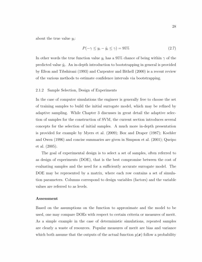
Figure 2.1: Three variants of factorial designs in three-dimensional design space.Samples are denoted by solid black dots.

Factorial Designs

Full factorial designs are likely the simplest space filling designs. For each parameter

a set of values is selected and the DOE consists simply of every possible combination,

forming a grid spanning the design space. For example Figure 2.1a shows a full

factorial design with two levels in a three-dimensional design space. Two and three

levels per variable are most common and the assumption is that this provides enough

information to discover linear and quadratic dependencies. The number of samples

is an exponential function of the number of levels, therefore full factorial designs are

generally not practical for high-dimensional problems. A possible solution is to use

fractional factorial designs such as Plackett-Burman designs (Plackett and Burman

(1946)) which leave out some of the samples. Figure 2.1b) shows a half-fractional

design consisting of half as many samples as the corresponding full factorial design.

Another variation of the factorial design is the central composite design (CCD)

(Figure 2.1c), which may be considered as a compromise between 2- and 3-level full

factorial designs. A thorough introduction to full and fractional factorial designs

and their variations is given by Myers et al. (2009) for example.

31

x1

x2

(a) LHS design 1

x1

x2

(b) LHS design 2

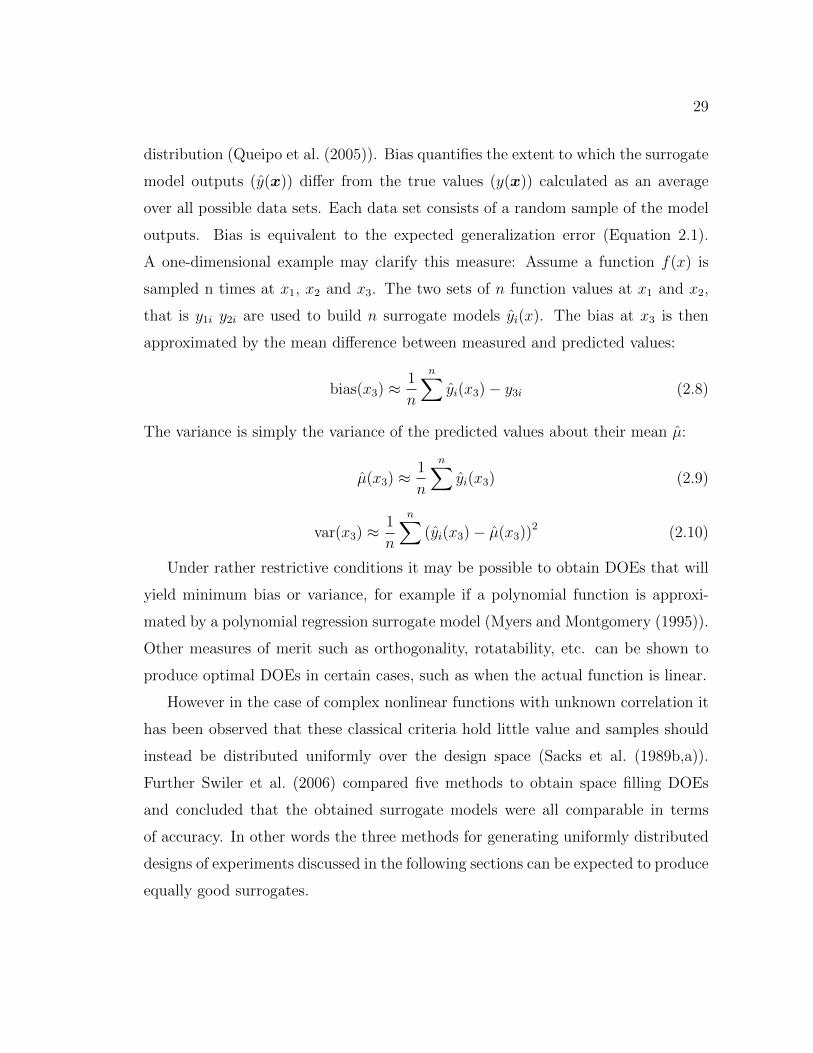
Figure 2.2: Two examples of latin hypercube sampling with 9 levels in a two-dimensional design space. In each design, none of the 9 segments is sampled twice.

Latin Hypercube Sampling (LHS)

A latin hypercube sampling (McKay et al. (1979)) is obtained by dividing each

parameter range into n segments of equal probability. n samples are composed

randomly such that each segment is sampled once and no two samples contain the

same level for any of the factors as shown by two examples of LHS in Figure 2.2.

In the case where the parameters are not random variables, n equally spaced values

are selected for each parameter. Latin hypercube sampling has been used for over

thirty years and this standard procedure is covered by most texts on computer

experiments.

Advantages of LHS are the simplicity of the algorithm which allows to gener-

ate large DOEs very efficiently as compared to central voronoi tesselation (Section

2.1.2). Also unlike factorial designs (Section 2.1.2) any number of samples may be

generated. A possible disadvantage of LHS is that it can be lacking in terms of

uniformity as measured by maximum minimum-distance between samples (Queipo

et al. (2005)). This has been addressed by various optimized LHS (Ye et al. (2000);

Viana et al. (2010)).

32

x1

x2

(a) CVT design: 10 samples

x1

x2

(b) CVT design: 11 samples

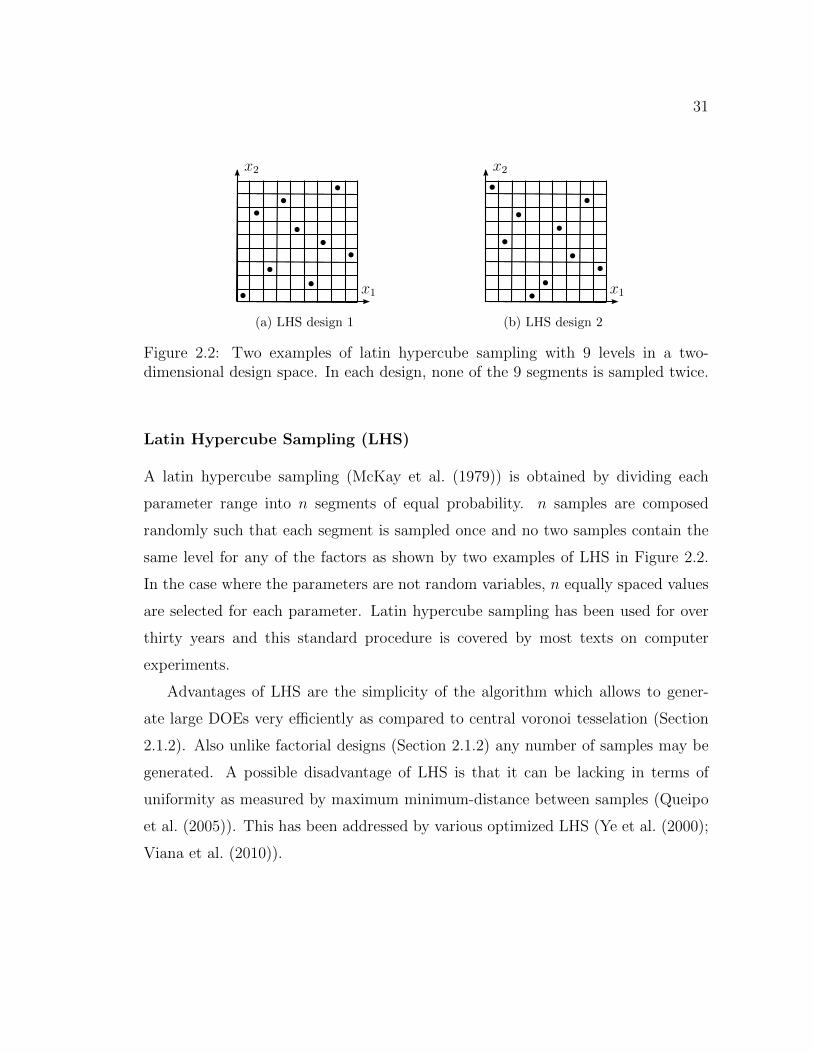
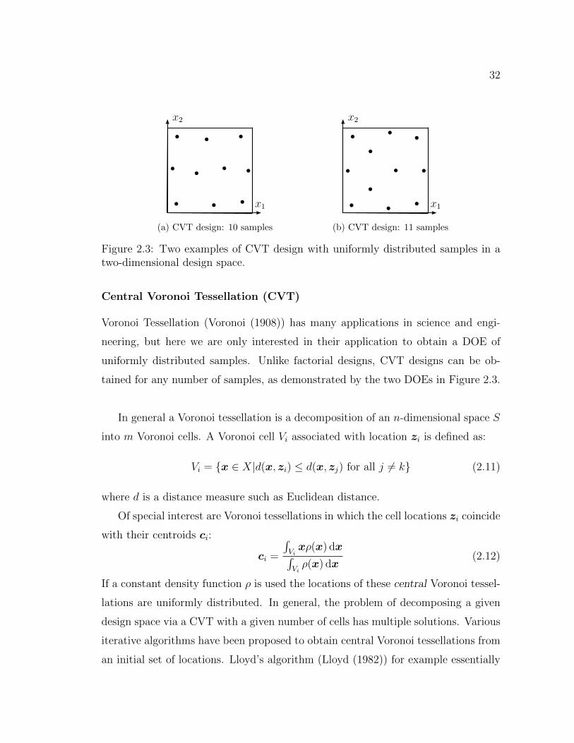
Figure 2.3: Two examples of CVT design with uniformly distributed samples in atwo-dimensional design space.

Central Voronoi Tessellation (CVT)

Voronoi Tessellation (Voronoi (1908)) has many applications in science and engi-

neering, but here we are only interested in their application to obtain a DOE of

uniformly distributed samples. Unlike factorial designs, CVT designs can be ob-

tained for any number of samples, as demonstrated by the two DOEs in Figure 2.3.

In general a Voronoi tessellation is a decomposition of an n-dimensional space S

into m Voronoi cells. A Voronoi cell Vi associated with location zi is defined as:

Vi = {x ∈ X|d(x, zi) ≤ d(x, zj) for all j 6= k} (2.11)

where d is a distance measure such as Euclidean distance.

Of special interest are Voronoi tessellations in which the cell locations zi coincide

with their centroids ci:

ci =

∫Vixρ(x) dx∫

Viρ(x) dx

(2.12)

If a constant density function ρ is used the locations of these central Voronoi tessel-

lations are uniformly distributed. In general, the problem of decomposing a given

design space via a CVT with a given number of cells has multiple solutions. Various

iterative algorithms have been proposed to obtain central Voronoi tessellations from

an initial set of locations. Lloyd’s algorithm (Lloyd (1982)) for example essentially

33

consists of replacing the cell locations by their closest centroid at each iteration. A

concise summary of CVT and it’s applications is offered by Du et al. (1999). A very

comprehensive treatment is the classical text Okabe et al. (1992).

2.1.3 Polynomials

While the more powerful surrogate models of radial basis functions and Kriging

discussed in later sections are relatively recent developments, polynomial functions

were among the first surrogate models. These surrogate models are parameterized

in terms of the polynomial coefficients, and searching for the parameters that give

the closest fit to a given set of results is known as regression.

This section provides a brief summary of the fundamentals of polynomial sur-

rogate models. Various review articles offer concise introductions (Forrester and

Keane (2009); Simpson et al. (2001); Queipo et al. (2005)) and in-depth coverage is

provided by many text books such as the classic Box and Draper (1987).

In the case of a single variable, a polynomial surrogate model of degree m is

given as:

y(x) =m∑i=0

βixi (2.13)

In the n-dimensional case the most-common polynomials of degree 1 and 2 are:

y(x) = β0 +n∑i=1

βixi (2.14)

y(x) = β0 +n∑i=1

βixi +n∑i=1

j∑i=1

βijxixj (2.15)

Given a set of s samples xi the predictions yi may be written in matrix form as:

y = Φβ (2.16)

where β contains all the coefficients and y is a column vector of predictions. In the

34

one-dimensional case Φ is the Vandermonde matrix:

Φ =

1 x1 x21 . . . xm1

1 x2 x22 . . . xm2...

......

. . ....

1 xs x2s . . . xms

(2.17)

In the n-dimensional case Φ also contains mixed terms. Assuming that the number

of samples s exceeds the number of coefficients, the coefficients can be determined

uniquely by minimizing the quadratic prediction error:

β = arg minβ

1

s

s∑||y − y||2 (2.18)

The quadratic loss function is differentiable (Section 2.1.1) and the coefficients are

obtained by setting the derivative of the sum of errors to zero. This results in a

linear equation for β with the solution:

β =(ΦTΦ

)−1y (2.19)

The degree m of the polynomial surrogate may be selected based on minimum

estimated generalization error using, for example, cross-validation 2.1.1. Alterna-

tively one may use the null-hypothesis under which the degree is increased as long

as the improvement of a scaled error measure is significant (Ralston and Rabinowitz

(1978)).

In theory any continuous function is approximated to arbitrary accuracy by a

Taylor series of high enough order, but in practice polynomial surrogate models are

ill-suited for highly non-linear models. Since the polynomial itself is smooth, trying

to approximate a discontinuous response via a polynomial surrogate via Equation

2.18 will always produce a poor fit, not necessarily limited to the discontinuity.

In high dimensions only low order polynomials may be feasible due to the large

number of coefficients. Additional concerns are the oscillatory shape of high degree

polynomials and numerical stability.

35

2.1.4 Radial Basis Functions

Here a weighted sum of simple basis functions is used to approximate the function of

interest based on a set of n evaluated samples xi and corresponding function values

yi = f(xi) (Broomhead and Lowe (1988)). The surrogate model f(x) is constructed

as:

f(x) =n∑i=1

wiψ (‖x− xi‖) (2.20)

with weights wi and radial basis function ψ. The function argument ‖x−xi‖ equals

the distance to the training sample xi as is often referred to as radius. Equation 2.20

is so general that it encompasses several popular surrogate models. For example,

splines can be represented as radial basis functions if the basis function is selected

properly. Similarly, single layer neural networks with radial coordinate neurons may

be represented by equation 2.20 (Duch and Jankowski (1999)). Kriging models

however do not conform to equation 2.20 since their basis function is not a function

of euclidean distance. The basis function ψ(r) may be fixed or parametric and some

popular choices are (Forrester and Keane (2009)):

• linear ψ(r) = r

• cubic ψ(r) = r3

• thin plate spline ψ(r) = r2 ln(r)

• Gaussian ψ(r) = e−r2/2σ2

• multi-quadratic ψ(r) = (r2 + σ)1/2

• inverse multi-quadratic ψ(r) = (r2 + σ)−1/2

In general parametric kernels may lead to better approximations with fewer samples

if the parameters are chosen wisely. However estimation of the parameters such as σ,

based on for example cross-validation (Friedman et al. (2001)), will add considerable

over-head and therefore fixed basis functions may be a better choice.

36

For a given basis function the weightsw are obtained by solving the interpolation

condition 2.21 which can also be stated in matrix form 2.22:

f(x) =n∑i=1

wiψ (||x− xi||) = yi) (2.21)

Ψw = y (2.22)

Often the number of basis function is chosen to match the number of evaluated

samples and then the interpolation condition is easily solved for w. In the case of

Gaussian and inverse multi-quadratic basis functions Ψ will be symmetric positive-

definite enabling computation of w via Cholesky factorization (Vapnik (1998)). Fur-

ther, in the case of Gaussian kernels the mean squared error of the prediction is

approximated as

MSE (x) =√

1−ψ(x)TΨ−1ψ(x) (2.23)

as derived in detail in Sobester (2003); Gibbs (1997).

If the evaluated samples are known to contain “noise”, then an exact interpo-

lation is known as overfitting and results in poor generalization of the model. To

avoid overfitting, only a small number of basis function may be selected via support

vector regression (Section 2.1.6). Alternatively a regularization parameter λ may

be introduced (Keane and Nair (2005)):

(Ψ + λI)w = y (2.24)

With the resulting weights of the RBF function given by the least-squares solution

of the above equation. If it is known, λ should be set to the standard deviation of

the noise (Keane and Nair (2005)).

2.1.5 Kriging

The concept of Kriging was introduced by Danie G. Krige to model geospacial dis-

tributions with the goal of selecting the most promising locations for mining (Krige

(1951)). A detailed history of the origins of Kriging is given by Cressie (1990). Krig-

ing was first proposed as a surrogate model of deterministic simulations by Sacks

37

et al. (1989b) and is now widely used for this purpose (Kleijnen (2009)). The pop-

ularity of Kriging is founded in part in the generality of the approach as the only

assumption about the approximated function is its continuity. On the other hand

the large number of parameters to be estimated create considerable overhead and

Kriging is therefore best suited to replace relatively expensive simulations. For the

same reason it is rarely used for problems with more than 20 variables (Forrester

and Keane (2009)). The availability of the estimated prediction error is very helpful

to select additional samples to refine the model. The model parameters, estimated

based on statistical analysis of the training data, may provide valuable information

about the actual function, especially for high-dimensional problems where the re-

sponse values are not easily visualized. For example, parameter θk can be used to

identify the most important variables (Keane (2003)) and exponent pk characterizes

the smoothness of the response (see Equation 2.30).

Concept

The basic assumption in Kriging is that the unknown function y(x) can be approx-

imated by the sum of global trend f(x) and local deviation Z(x).

y(x) ≈ f(x) + Z(x) (2.25)

f(x) known polynomial (global function), often constant (Sacks et al. (1989b); Welch

et al. (1990, 1992)). Working with f(x) equal to the mean value µ may be referred

to as ordinary Kriging and instead using some known function is referred to as

universal Kriging (Cressie (1993)). The Gaussian process Z(x) is characterized by

its variance σ2, and non-zero covariance, defined in the following paragraphs.

Variance, often denoted as σ2, is a measure of the variation in the values of the

random variable X and is defined as the expected value of squared deviation from

the expected value of X (E[X]).

Var(X) = σ2 = E[(X − E[X])2] (2.26)

It is of course closely related to another common measure of variation called standard

deviation σ (also called root mean square deviation).

38

Covariance is a measure of the dependence between two random variables (X

and Y ):

Cov(X, Y ) = E[(X − E[X])(Y − E[Y ])] (2.27)

For example, Cov(X, Y ) > 0 signifies that X is more likely to be above average if

Y is above average, while Cov(X, Y ) < 0 suggests an inverse relationship. How-

ever, covariance detects only linear dependence and one cannot conclude that two

variables are independent based on their covariance.

While closely related, correlation is a better measure of the strength of the linear

dependence since it is scaled by the product of standard deviations:

Corr(X, Y ) = Cov(X, Y )/(σXσY ) (2.28)

The value of correlation ranges from −1 to 1, where |Corr(X, Y )| = 1 signifies a

perfectly linear relationship between the two variables.

Model Construction

Based on training samples xi the correlation R matrix of the Gaussian process Z is

defined as:

Rij = Corr(Z(xi), Z(xj)) =1

σ2Cov(Z(xi), Z(xj)) (2.29)

The correlation function Rij is generally not known and therefore assumed to be of

the form:

Rij = exp

(−

d∑k=1

θk|xik − xjk|pk)

(2.30)

where d is the dimensionality of the design space. This continuous function equals

1 for xi = xj and approaches 0 as distance ‖xi −xj‖ approaches infinity. For large

values of θ function values change rapidly even over small distances. Exponents

pk close to 2 characterize a smooth function, while pk close to zero point to rough,

nondifferentiable functions. (Jones (2001))

The parameters µ, σ, θk and pk are selected to maximize the likelihood 2.31 of

the observed data. Given a set of n evaluated samples xi and corresponding function

39

values yi, then the log of the likelihood L of this outcome (without constant terms)

is:

log(L) = −n2

log(σ2)− 1

2log(|R|)− (y − 1µ)′R−1(y − 1µ)

2σ2(2.31)

A more in-depth presentation is given in Jones (2001). It is also common to

use simpler correlation modes where for example pk is fixed to 2 or only a single

θ is used on all dimensions (Sacks et al. (1989b,a); Koehler and Owen (1996)).

The boundaries between radial basis functions and Kriging are therefore fluid and

Kriging is sometimes considered a variation of radial basis functions.

Once the estimates for µ, σ, θk and pk are obtained they can be used to estimate

the likelihood of any outcome at any additional sample x∗. This yields not only the

expected value of y(x∗), but also its estimated probability density function. Both the

expected value y∗ and its mean square error (variance) are efficiently calculated in

closed form (Jones (2001)). One must be careful that the prediction error σ2 is only

an estimate based on estimated parameters and the whole process is based on the

assumption that the dependence between two samples is given by Equation 2.30. So

clearly, the estimated prediction error is not a reliable measure, but maybe helpful

for example to select additional samples. In particular, the estimated prediction

error plays an important role in the efficient global optimization (EGO) algorithm

presented in the following section.

Efficient Global Optimization (EGO)

This section offers a brief introduction to the efficient global optimization algorithm

which is closely tied to the Kriging approach. In the case of design optimization the

goal is to find the sample x∗ with the lowest function value y∗. Maybe the most

straight forward method is to use a sufficiently large number of samples to build the

surrogate model such that the generalization error (Section 2.1.1)is negligible for the

application. The surrogate is then used to find the location of the lowest predicted

function value, which may be evaluated to obtain the actual lowest function value

40

y∗. This is a very simple and robust algorithm, but due to the cost of evaluations, it

may be intractable. Fortunately lots of research effort has been directed at locating

the optimum design with much fewer sample evaluations.

A function may have several local optima, and surrogate-based optimization al-

gorithms may be divided into local algorithms that seek a local optimum in the

neighborhood of an initial design and global algorithms, developed to locate the

overall (global) optimum. Further one may distinguish between methods that can

take into account various design constraints and other algorithms specializing in

unconstrained problems. Another distinction is between algorithms geared towards

deterministic models versus random models. In general, global algorithms will eval-

uate an initial set of samples to obtain some initial knowledge about the function

behavior. During a second phase additional samples are selected iteratively to fur-

ther explore regions of interest. This is often referred to as adaptive sampling or

adaptive updating. The additional samples may be called infill points which are

selected based on infill criteria. A broad overview of recent progress in deterministic

global optimization is provided by Floudas and Gounaris (2009). A review of surro-

gate based infill criteria is presented by Forrester and Keane (2009). Not so recent,

but not at all outdated, Jones (2001) gives an excellent summary with particular fo-

cus on the failure modes of various Kriging-based methods for unconstrained global

optimization. Most recently Parr et al. (2012) gives a good summary of the latest

research regarding infill criteria.

This section only discusses in detail one global unconstrained optimization al-

gorithm based on Kriging surrogates and the maximum expected improvement cri-

terion often referred to as efficient global optimization (Jones et al. (1998)). The

presentation loosely follows Forrester and Keane (2009); Jones (2001).

Concept Initially a Kriging model is build from a relatively small set of evaluated

samples. At each subsequent iteration another sample is selected at maximum ex-

pected improvement to update the Kriging model. The expected improvement infill

criterion may be calculated for any point in the design space based on the predicted

41

value and estimated prediction error of the Kriging model as detailed in the follow-

ing paragraph. Various global optimization algorithms such as genetic programming

may be used to find the infill point with maximum expected improvement. Due to

the low cost of evaluating the criterion the choice of algorithm is not critical and is

not treated in this section.

Expected Improvement is estimated based on the assumption that the true func-

tion value at any point follows a normal distribution with variance s and mean y(x):

P (−∞ <y(x)− y(x)

s(x)≤ u) = Φ(u) =

1√2π

∫ u

−∞exp

(−t2

2

)dt (2.32)

Where Φ(u) is the standard normal cumulative distribution function. If n samples xi

have been evaluated and the best (lowest) function value is ymin then the estimated

probability that the actual function value at x will be lower is given by:

P (y(x) ≤ ymin) = Φ

(ymin − y(x)

s(x)

)(2.33)

The improvement over the current best sample is defined as:

I =

ymin − y(x) if y(x) < ymin

0 otherwise(2.34)

The probability density function of improvement is a normal probability density

function:1√

2πs(x)exp

(−(ymin − I − y(x))2

2s2(x)

)(2.35)

and finally the inspected improvement is obtained by integration:

E(I) =

∫ I=∞

I=0

1√2πs(x)

exp

(−(ymin − I − y(x))2

2s2(x)

)dI (2.36)

The choice of convergence criterion to decide when to terminate the sampling

process is always subjective and application dependent. A natural choice seems to

stop the algorithm when the expected improvement is below a certain threshold. The

threshold should be selected rather conservatively since the expected improvement

is only an estimate. In particular Cressie (1993) shows that the prediction error

42

tends to be underestimated, which leads to unrealistically low estimates of expected

improvement. In practical applications the number of iterations may be dictated by

design schedules and computational resources.

The presented algorithm is considered a two-stage approach, where the first

stage of each iteration consists of estimating the parameters of the Kriging model.

The second stage relies on the accuracy of the estimated parameters to select an

additional sample for evaluation. This reliance on possibly poor estimates creates

various pitfalls and failure modes discussed in detail by Jones (2001). In particular

the estimate of prediction error is prone to inaccuracy as pointed out by Den Hertog

et al. (2005); Cressie (1993). Various alternative estimates of the variance based on

bootstrapping are proposed by Den Hertog et al. (2005) and Kleijnen et al. (2012)

shows how these may lead to better estimates of expected improvement. In most

cases the pitfalls of the presented two-stage algorithm can be avoided by choosing

a large enough set of initial samples. Alternatively one-stage algorithms have been

proposed (Gutmann (2001); Jones (2001); Forrester and Jones (2008)) where the

likelihood of a certain function value at an additional sample is evaluated based on

training a new Kriging model passing through that point. In theory these one-stage

algorithms may be the “silver bullet” of numerical optimization with surrogates,

but they are also much more computationally intense and may only be practical

for applications with extremely expensive model evaluations (Forrester and Keane

(2009)).

2.1.6 Support Vector Regression

Support Vector Regression may be considered as a special case of radial basis func-

tions, where only a subset of the evaluated samples is used to construct the surrogate.

With reference to Equation 2.20 the number of bases nb is much smaller than the

number of evaluated samples ns. Historically support vector regression originates in

the theory of support vector machines (Vapnik (1995)), which are covered in detail

in Section 2.4

Similar to radial basis functions the support vector regression seeks an approxi-

43

mation model of the following form:

f(x) = µ+

nb∑i=1

wiψ (x,xsvi ) (2.37)

Here ψ(x,y) is referred to as kernel function and and the so-called support vectors

xsvj are a subset of the evaluated samples xi. The weights wi and support vectors

are selected to minimize an objective function defined in terms of w, penalized by

constraints on the approximation error at the evaluated samples:

w = arg minw

1

2‖w‖2 + C

ns∑i=1

L(f(xi), yi) (2.38)

Here C > 0 is the penalty factor and L is the ε-insensitive loss function introduced

in Section 2.1.1:

L(f1, f2) =

0 if |f1 − f2| < ε

|f1 − f2| − ε otherwise(2.39)

and support vectors are characterized by wi 6= 0. The cost function only penalizes

deviations larger than ε and minimizing ‖w‖2 may be seen as a way of minimizing

model complexity (Forrester and Keane (2009)). Figure 2.4 shows an example of a

one-dimensional SVR surrogate model based on a number of training samples.

The parameters ε and C may be chosen based on prior knowledge about the

noise in the response values yi, but that is generally not available. Alternatively

cross-validation can be employed to compare ε, C pairs in order to find the best

values. The accuracy of the support vector regression is not very sensitive to the

choice of parameters and a simple grid search often yields good results.

An in-depth introduction to SVR is given by Scholkopf and Smola (2001). SVR

is compared to other surrogate models on 26 engineering test problems by Clarke

et al. (2005) and it was found that though Kriging may result in slightly lower

generalization error, SVR appears to be more robust. Other empirical studies of the

performance of SVR showed very promising results as well (Gunn (1998); Vapnik

et al. (1996)). Though Kriging appears to be the surrogate model of choice for

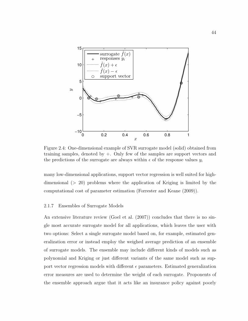
44

0 0.2 0.4 0.6 0.8 1−10

−5

0

5

10

15

x

y

surrogate f(x)responses yif(x) + ǫ

f(x)− ǫ

support vector

Figure 2.4: One-dimensional example of SVR surrogate model (solid) obtained fromtraining samples, denoted by +. Only few of the samples are support vectors andthe predictions of the surrogate are always within ε of the response values yi

many low-dimensional applications, support vector regression is well suited for high-

dimensional (> 20) problems where the application of Kriging is limited by the

computational cost of parameter estimation (Forrester and Keane (2009)).

2.1.7 Ensembles of Surrogate Models

An extensive literature review (Goel et al. (2007)) concludes that there is no sin-

gle most accurate surrogate model for all applications, which leaves the user with

two options: Select a single surrogate model based on, for example, estimated gen-

eralization error or instead employ the weighed average prediction of an ensemble

of surrogate models. The ensemble may include different kinds of models such as

polynomial and Kriging or just different variants of the same model such as sup-

port vector regression models with different ε parameters. Estimated generalization

error measures are used to determine the weight of each surrogate. Proponents of

the ensemble approach argue that it acts like an insurance policy against poorly

45

fitted models (Viana et al. (2009)) and will improve the robustness of surrogate-

based optimization (Glaz et al. (2009); Saijal et al. (2011)). On the other hand

Viana et al. (2009) also concedes that while in theory the most accurate surrogate

can be beaten by an ensemble, this is very difficult in practice, especially in high

dimensions. Most likely the most complete and up to date review of the ensemble

approach is provided by Viana (2011). In conclusion one may argue that ensem-

bles of surrogates may become increasingly popular with the availability of more

computational power and better software, when the added cost of training multiple

surrogates become negligible.

2.2 Multi-Fidelity Techniques

The last 25 years have seen a major increase in publications on multi-fidelity methods

for computational design. These methods use at least two models for the evaluation

of designs: The high-fidelity model provides the reference in terms of accuracy and

the low-fidelity model produces less accurate response values, but at significantly

lower expense. In part these methods are a formalization of long-since established

design practices: Engineers have always used simpler approximations for preliminary

design or to rule out flagrantly inadequate designs. With the exponential increase

in computational capabilities of previous decades, state of the art simulation models

have become ever more sophisticated and powerful, but it is often observed that the

highest accuracy available is rarely required. In addition, modern algorithms for

numerical optimization and uncertainty quantification often require the evaluation

of massive numbers of similar designs, which is simply not feasible at the highest

level of fidelity. This situation creates the challenge of using various levels of analysis

fidelity most efficiently to free up resources for cheaper and faster design processes

or to investigate more alternative designs.

Section 2.2.1 discusses the benefits of building a preliminary response surface

based on a low-fidelity approximation. Section 2.2.2 summarizes several algorithms

to obtain a surrogate of the high-fidelity response model from a low-fidelity model

46

and additional high-fidelity training samples, referred to as model correction. Such

modified low-fidelity models that are fitted to locally match the high-fidelity response

are at the backbone of the multi-fidelity trust region optimization method reviewed

in Section 2.2.3

2.2.1 Preliminary Low-Fidelity Study

Most simulation models have some straight-forward fidelity parameters which affect

both accuracy and computational cost of the simulations. Examples of such parame-

ters, which often relate to discretization, are finite element mesh size, integrator step

size, number of Monte-Carlo samples, etc. When given such a model to investigate

parameterized designs, it is customary to start with a relatively low fidelity setting

to gain some preliminary insight into the model behavior. This is generally helpful

to identify regions in the design space of particular interest and these low-fidelity

results may also serve as a baseline to later determine convergence of the results

with higher fidelity settings. For the purpose of design optimization the low-fidelity

simulation model or a corresponding surrogate model may be used to identify “non-

sense regions” which should be ignored because they are clearly far from optimal, as

demonstrated on aerodynamic wing design (Giunta et al. (1995a,b)). In addition the

low-fidelity response surface may be used to study the “make up” of the function,

possibly identifying intervening functions that compose the model and are easier to

approximate (Kaufman et al. (1996)).

2.2.2 Low-Fidelity Model Correction

Section 2.1 discusses general purpose surrogate models and it is reported that dif-

ferent models are better for different problems and that it is very difficult to predict

which surrogate will perform best for a given response model. However, in the

case of multi-fidelity models, one can use the lower-fidelity model to help in the

approximation of the higher-fidelity model. It is often reasonable to assume that a

surrogate model that approximates the low-fidelity model efficiently will also per-

47

form well on the high-fidelity model, therefore low-fidelity samples can be used to

select a suitable surrogate and corresponding parameters to approximate the high-

fidelity model. In other words, domain-specific information from the low-fidelity

model leads to improvements in the high-fidelity model approximation.

It has been observed in the field of empirical model building that carefully

constructed, special-purpose approximation models (also referred to as mechanis-

tic models) generally outperform the general-purpose models discussed in Section

2.1 (Box and Draper (1987)). In the case of multi-fidelity analysis we have the

domain-specific knowledge to build such a specialized model and several approaches

have been suggested to build an approximation fH(x) of the high-fidelity fH(x)

model based on the low-fidelity model fL(x) and additional parameters a as:

fH(x) ≈ f(fL(x),a) (2.40)

In the following paragraphs the four most popular formulations for constructing

this high-fidelity surrogate will be discussed. Which of these methods is best for

a given scenario is problem dependent and may be decided based on experience

or approximated generalization error (Section 2.1.1). Alternatively an ensemble of

surrogates may be used (Section 2.1.7).

Additive correction consists of approximating the difference in response values

between the high-fidelity and the low-fidelity response values (Equation 2.41). This

correction function C(x,a) may be as simple as a constant or as sophisticated as a

Kriging model (Keane (2003)):

fH(x) = C(x,a) + fL(x) (2.41)

Additive Correction has been used successfully during a wing optimization problem

by Keane (2003), but it appears that scaling as described in the following paragraph

is considerably more popular.

Scaling uses a factor to match the low-fidelity model to the high-fidelity outputs:

fH(x) = C(x,a)fL(x) (2.42)

48

The approach is of course general and any surrogate maybe used to construct the

correction function C(x,a), but a particularly popular approach is to use a first

order Taylor series of the ratio of response values β (Alexandrov et al. (2001)):

β(x) =fH(x)

fL(x)(2.43)

This results in an approximation fH that matches the high-fidelity model in value

and gradient at a single point. It was first demonstrated in the Global-Local Ap-

proximation method (GLA) to match a coarse FE beam model (low fidelity) to

the results of a more refined FE model (Haftka (1991)) and later employed dur-

ing aerodynamic and structural optimization (Unger et al. (1992); Chang et al.

(1993); Hutchison et al. (1994); Alexandrov et al. (2000, 2001); Gano et al. (2005,

2006)) using Variable Complexity Modeling (VCM) and Approximation Manage-

ment Framework (AMF). Eldred et al. (2004); Eldred and Dunlavy (2006) proposed

the use of second order Taylor series and compares this approach to other surrogate

models. All of these methods have in common that the high-fidelity approximation

fH(x) is used as part of a gradient-based optimization routine to obtain a local opti-

mum. For this purpose the high-fidelity approximation was repeatedly constructed

to match both value and gradients of the high-fidelity model at the current iterate.

A possible disadvantage of the multiplicative corrective function is the singularity

if fL(x) = 0.

A more “intrusive” approach is termed parameter tuning. Here a set of param-

eters a of the low-fidelity model are set to fit the low-fidelity output to high-fidelity

response values:

fH(x) = fL(x,a) (2.44)

Often the low-fidelity model is specifically constructed for this purpose, for example

Toropov et al. (1997) simulated a mechanical system with rigid bodies and used

the mass distributions as artificial parameters to match simulation results of the

same system with flexible members. Berci et al. (2011) used parameter tuning to

model the gust response of a very flexible wing and Toropov and Van der Giessen

(1993) approximated nonlinear deformations of a solid bar specimen. The parameter

49

tuning approach is most promising if the simulated system is well understood and

not suitable for black-box models. If available, parameter tuning appears to be

the most efficient model correction method as found in several comparative studies

(Toropov et al. (1997); Berci et al. (2009, 2011)).

Space mapping is another model correction method that modifies the input of

the low-fidelity model to match its outputs to the high-fidelity responses. Instead

of model parameters, the design variables are transformed via a linear or nonlin-

ear mapping function C(x,a) such that the deviation of the low-fidelity model is

minimized:

fH(x) = fL(C(x,a)) (2.45)

Space mapping is often compared to drawing the contours of the low-fidelity response

on a rubber sheet, which is then distorted to match the high-fidelity contours (Keane

and Nair (2005)), but space mapping is of course applicable to higher dimensional

design spaces as well. Space mapping is a standard tool in microwave circuit design

(Bandler et al. (2004); Koziel et al. (2008)) and has been gaining popularity in

other areas of design, such as structural optimization (Leary et al. (2003); Redhe

and Nilsson (2006)). In general, the low-fidelity model and the high-fidelity model

may have different design spaces, that is the design variables may be different in type

and number. This issue was addressed via corrected space mapping proposed by

Robinson et al. (2006b,a); Robinson (2007); Robinson et al. (2008) as demonstrated

on wing design and flapping wing problems.

The low-fidelity model is often a surrogate fitted to low-fidelity training samples,

therefore instead of applying a correction to the low-fidelity model, one may apply

a correction to the low-fidelity training samples to obtain an approximation of high-

fidelity response model. This was investigated by Balabanov et al. (1998) and it was

found that the difference was rather small.

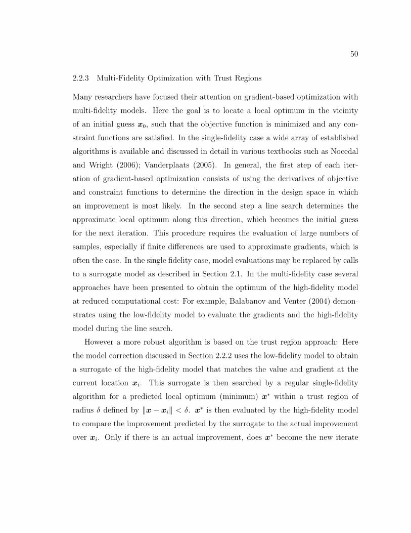
50

2.2.3 Multi-Fidelity Optimization with Trust Regions

Many researchers have focused their attention on gradient-based optimization with

multi-fidelity models. Here the goal is to locate a local optimum in the vicinity

of an initial guess x0, such that the objective function is minimized and any con-

straint functions are satisfied. In the single-fidelity case a wide array of established

algorithms is available and discussed in detail in various textbooks such as Nocedal

and Wright (2006); Vanderplaats (2005). In general, the first step of each iter-

ation of gradient-based optimization consists of using the derivatives of objective

and constraint functions to determine the direction in the design space in which

an improvement is most likely. In the second step a line search determines the

approximate local optimum along this direction, which becomes the initial guess

for the next iteration. This procedure requires the evaluation of large numbers of

samples, especially if finite differences are used to approximate gradients, which is

often the case. In the single fidelity case, model evaluations may be replaced by calls

to a surrogate model as described in Section 2.1. In the multi-fidelity case several

approaches have been presented to obtain the optimum of the high-fidelity model

at reduced computational cost: For example, Balabanov and Venter (2004) demon-

strates using the low-fidelity model to evaluate the gradients and the high-fidelity

model during the line search.

However a more robust algorithm is based on the trust region approach: Here

the model correction discussed in Section 2.2.2 uses the low-fidelity model to obtain

a surrogate of the high-fidelity model that matches the value and gradient at the

current location xi. This surrogate is then searched by a regular single-fidelity

algorithm for a predicted local optimum (minimum) x∗ within a trust region of

radius δ defined by ‖x− xi‖ < δ. x∗ is then evaluated by the high-fidelity model

to compare the improvement predicted by the surrogate to the actual improvement

over xi. Only if there is an actual improvement, does x∗ become the new iterate

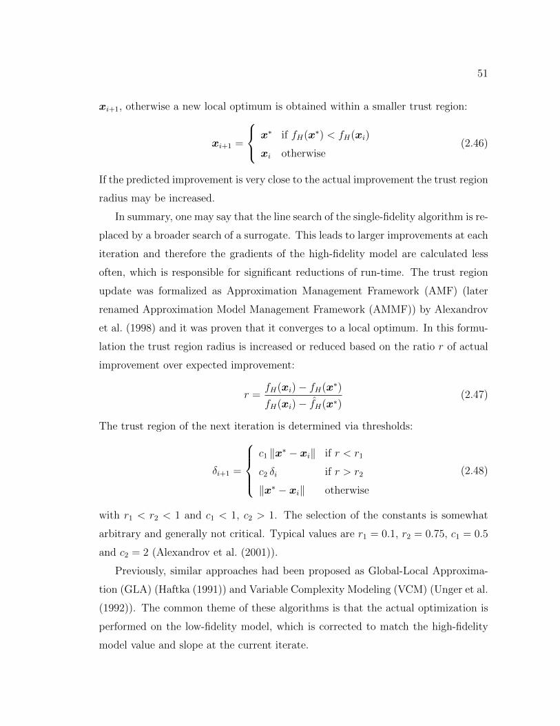
51

xi+1, otherwise a new local optimum is obtained within a smaller trust region:

xi+1 =

x∗ if fH(x∗) < fH(xi)

xi otherwise(2.46)

If the predicted improvement is very close to the actual improvement the trust region

radius may be increased.

In summary, one may say that the line search of the single-fidelity algorithm is re-

placed by a broader search of a surrogate. This leads to larger improvements at each

iteration and therefore the gradients of the high-fidelity model are calculated less

often, which is responsible for significant reductions of run-time. The trust region

update was formalized as Approximation Management Framework (AMF) (later

renamed Approximation Model Management Framework (AMMF)) by Alexandrov

et al. (1998) and it was proven that it converges to a local optimum. In this formu-

lation the trust region radius is increased or reduced based on the ratio r of actual

improvement over expected improvement:

r =fH(xi)− fH(x∗)

fH(xi)− fH(x∗)(2.47)

The trust region of the next iteration is determined via thresholds:

δi+1 =

c1 ‖x∗ − xi‖ if r < r1

c2 δi if r > r2

‖x∗ − xi‖ otherwise

(2.48)

with r1 < r2 < 1 and c1 < 1, c2 > 1. The selection of the constants is somewhat

arbitrary and generally not critical. Typical values are r1 = 0.1, r2 = 0.75, c1 = 0.5

and c2 = 2 (Alexandrov et al. (2001)).

Previously, similar approaches had been proposed as Global-Local Approxima-

tion (GLA) (Haftka (1991)) and Variable Complexity Modeling (VCM) (Unger et al.

(1992)). The common theme of these algorithms is that the actual optimization is

performed on the low-fidelity model, which is corrected to match the high-fidelity

model value and slope at the current iterate.

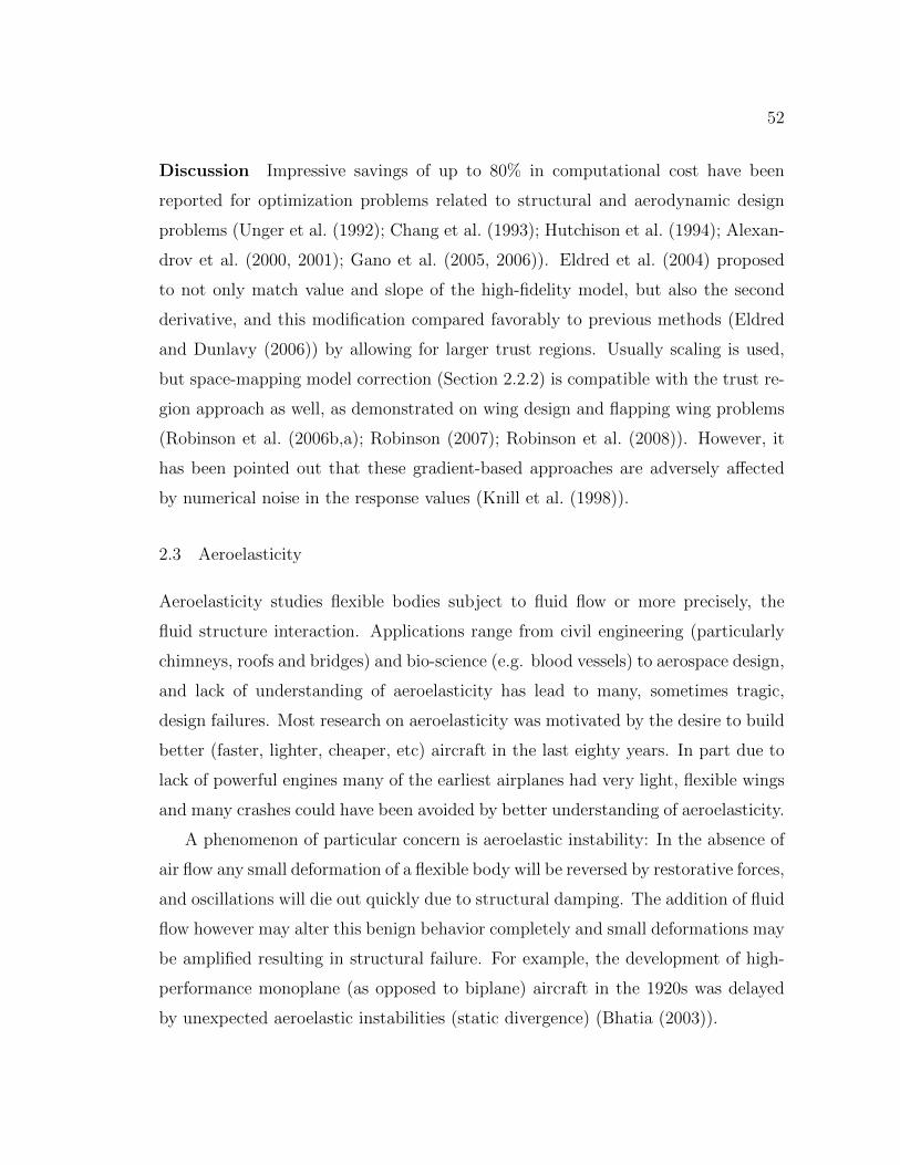
52

Discussion Impressive savings of up to 80% in computational cost have been

reported for optimization problems related to structural and aerodynamic design

problems (Unger et al. (1992); Chang et al. (1993); Hutchison et al. (1994); Alexan-

drov et al. (2000, 2001); Gano et al. (2005, 2006)). Eldred et al. (2004) proposed

to not only match value and slope of the high-fidelity model, but also the second

derivative, and this modification compared favorably to previous methods (Eldred

and Dunlavy (2006)) by allowing for larger trust regions. Usually scaling is used,

but space-mapping model correction (Section 2.2.2) is compatible with the trust re-

gion approach as well, as demonstrated on wing design and flapping wing problems

(Robinson et al. (2006b,a); Robinson (2007); Robinson et al. (2008)). However, it

has been pointed out that these gradient-based approaches are adversely affected

by numerical noise in the response values (Knill et al. (1998)).

2.3 Aeroelasticity

Aeroelasticity studies flexible bodies subject to fluid flow or more precisely, the

fluid structure interaction. Applications range from civil engineering (particularly

chimneys, roofs and bridges) and bio-science (e.g. blood vessels) to aerospace design,

and lack of understanding of aeroelasticity has lead to many, sometimes tragic,

design failures. Most research on aeroelasticity was motivated by the desire to build

better (faster, lighter, cheaper, etc) aircraft in the last eighty years. In part due to

lack of powerful engines many of the earliest airplanes had very light, flexible wings

and many crashes could have been avoided by better understanding of aeroelasticity.

A phenomenon of particular concern is aeroelastic instability: In the absence of

air flow any small deformation of a flexible body will be reversed by restorative forces,

and oscillations will die out quickly due to structural damping. The addition of fluid

flow however may alter this benign behavior completely and small deformations may

be amplified resulting in structural failure. For example, the development of high-

performance monoplane (as opposed to biplane) aircraft in the 1920s was delayed

by unexpected aeroelastic instabilities (static divergence) (Bhatia (2003)).

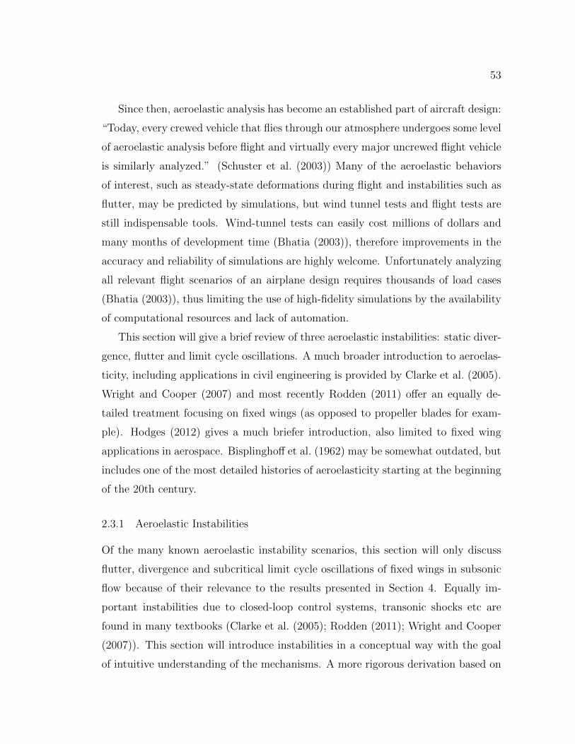
53

Since then, aeroelastic analysis has become an established part of aircraft design:

“Today, every crewed vehicle that flies through our atmosphere undergoes some level

of aeroelastic analysis before flight and virtually every major uncrewed flight vehicle

is similarly analyzed.” (Schuster et al. (2003)) Many of the aeroelastic behaviors

of interest, such as steady-state deformations during flight and instabilities such as

flutter, may be predicted by simulations, but wind tunnel tests and flight tests are

still indispensable tools. Wind-tunnel tests can easily cost millions of dollars and

many months of development time (Bhatia (2003)), therefore improvements in the

accuracy and reliability of simulations are highly welcome. Unfortunately analyzing

all relevant flight scenarios of an airplane design requires thousands of load cases

(Bhatia (2003)), thus limiting the use of high-fidelity simulations by the availability

of computational resources and lack of automation.

This section will give a brief review of three aeroelastic instabilities: static diver-

gence, flutter and limit cycle oscillations. A much broader introduction to aeroelas-

ticity, including applications in civil engineering is provided by Clarke et al. (2005).

Wright and Cooper (2007) and most recently Rodden (2011) offer an equally de-

tailed treatment focusing on fixed wings (as opposed to propeller blades for exam-

ple). Hodges (2012) gives a much briefer introduction, also limited to fixed wing

applications in aerospace. Bisplinghoff et al. (1962) may be somewhat outdated, but

includes one of the most detailed histories of aeroelasticity starting at the beginning

of the 20th century.

2.3.1 Aeroelastic Instabilities

Of the many known aeroelastic instability scenarios, this section will only discuss

flutter, divergence and subcritical limit cycle oscillations of fixed wings in subsonic

flow because of their relevance to the results presented in Section 4. Equally im-

portant instabilities due to closed-loop control systems, transonic shocks etc are

found in many textbooks (Clarke et al. (2005); Rodden (2011); Wright and Cooper

(2007)). This section will introduce instabilities in a conceptual way with the goal

of intuitive understanding of the mechanisms. A more rigorous derivation based on

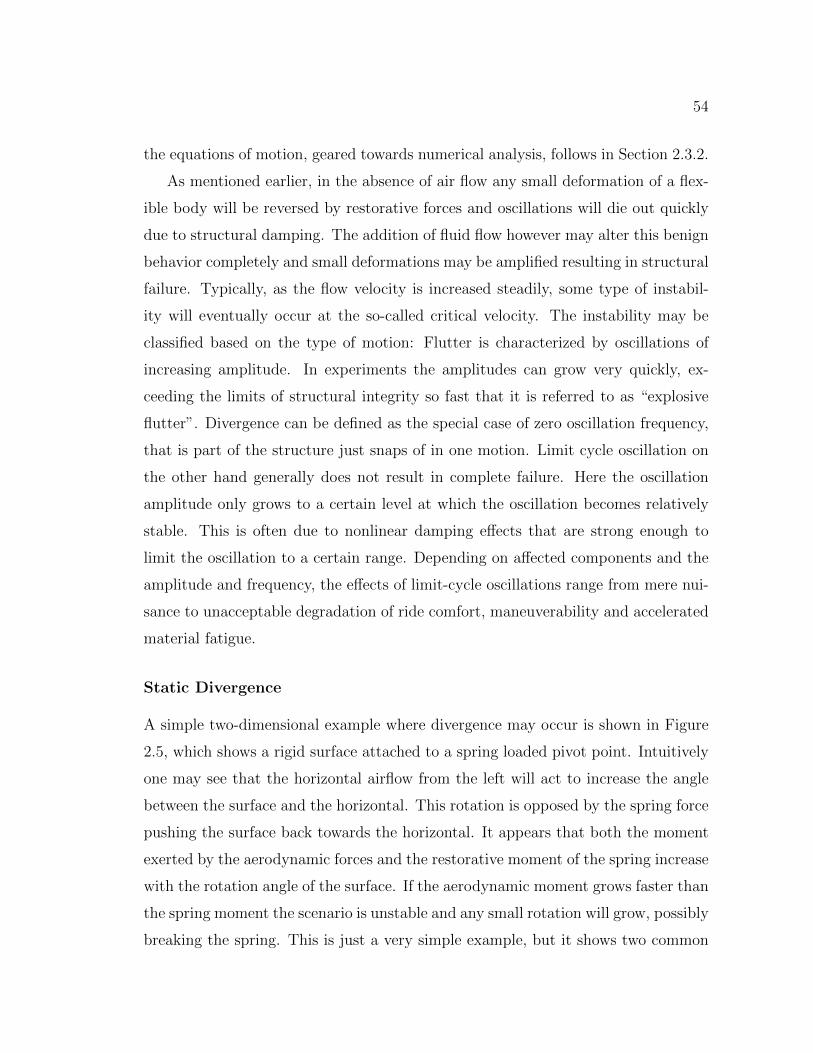
54

the equations of motion, geared towards numerical analysis, follows in Section 2.3.2.

As mentioned earlier, in the absence of air flow any small deformation of a flex-

ible body will be reversed by restorative forces and oscillations will die out quickly

due to structural damping. The addition of fluid flow however may alter this benign

behavior completely and small deformations may be amplified resulting in structural

failure. Typically, as the flow velocity is increased steadily, some type of instabil-

ity will eventually occur at the so-called critical velocity. The instability may be

classified based on the type of motion: Flutter is characterized by oscillations of

increasing amplitude. In experiments the amplitudes can grow very quickly, ex-

ceeding the limits of structural integrity so fast that it is referred to as “explosive

flutter”. Divergence can be defined as the special case of zero oscillation frequency,

that is part of the structure just snaps of in one motion. Limit cycle oscillation on

the other hand generally does not result in complete failure. Here the oscillation

amplitude only grows to a certain level at which the oscillation becomes relatively

stable. This is often due to nonlinear damping effects that are strong enough to

limit the oscillation to a certain range. Depending on affected components and the

amplitude and frequency, the effects of limit-cycle oscillations range from mere nui-

sance to unacceptable degradation of ride comfort, maneuverability and accelerated

material fatigue.

Static Divergence

A simple two-dimensional example where divergence may occur is shown in Figure

2.5, which shows a rigid surface attached to a spring loaded pivot point. Intuitively

one may see that the horizontal airflow from the left will act to increase the angle

between the surface and the horizontal. This rotation is opposed by the spring force

pushing the surface back towards the horizontal. It appears that both the moment

exerted by the aerodynamic forces and the restorative moment of the spring increase

with the rotation angle of the surface. If the aerodynamic moment grows faster than

the spring moment the scenario is unstable and any small rotation will grow, possibly

breaking the spring. This is just a very simple example, but it shows two common

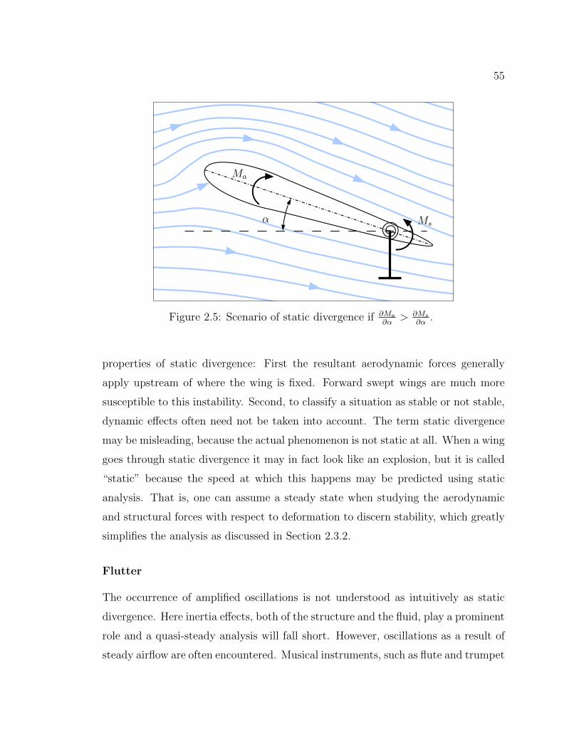
55

Ms

Ma

α

Figure 2.5: Scenario of static divergence if ∂Ma

∂α> ∂Ms

∂α.

properties of static divergence: First the resultant aerodynamic forces generally

apply upstream of where the wing is fixed. Forward swept wings are much more

susceptible to this instability. Second, to classify a situation as stable or not stable,

dynamic effects often need not be taken into account. The term static divergence

may be misleading, because the actual phenomenon is not static at all. When a wing

goes through static divergence it may in fact look like an explosion, but it is called

“static” because the speed at which this happens may be predicted using static

analysis. That is, one can assume a steady state when studying the aerodynamic

and structural forces with respect to deformation to discern stability, which greatly

simplifies the analysis as discussed in Section 2.3.2.

Flutter

The occurrence of amplified oscillations is not understood as intuitively as static

divergence. Here inertia effects, both of the structure and the fluid, play a prominent

role and a quasi-steady analysis will fall short. However, oscillations as a result of

steady airflow are often encountered. Musical instruments, such as flute and trumpet

56

use this effect to generate sounds. A flag “fluttering” in the wind is another example.

Flutter is often predicted based on linear models that assume displacements to be

small and do not take into account structural damping and other nonlinear effects.

If the system is unstable, small oscillations will quickly grow in amplitude and the

linear assumptions are no longer valid. At this point, two scenarios are possible:

• The oscillations continue to grow until structural failure occurs. This is gen-

erally referred to as flutter.

• Nonlinear effects provide sufficient damping to restrict the oscillations to a rel-

atively small, sustained amplitude. This is referred to as limit cycle oscillation

(LCO).

Under this definition, the examples of the fluttering flag and wind instruments would

be considered limit cycle oscillations, since they are obviously limited in amplitude

and do lead to structural failure. In terms of aerospace design, limit cycle oscillations

may be tolerated to some extend, but flutter must be avoided at all cost. Generally,

flutter predicted based on a linear model may turn out as limit cycle oscillation

in experiments. Rigorous analysis of flutter based on the equations of motion is

covered in Section 2.3.2.

Limit Cycle Oscillations (LCO)

As described in Section 2.3.1, limit cycle oscillation is a self-sustained vibration

of limited amplitude, which only occurs in nonlinear systems. It is usually not a

dramatic event, but LCO might hamper, for instance, control and maneuverability

and has therefore emerged as an interesting design challenge (Kousen and Bendiksen

(1994); Dowell and Tang (2002)). From a design point of view, the challenge lies in

developing approaches to manage LCO and mitigate their effects in a way prescribed

by the designer.

It is commonly accepted that two situations might be associated with LCO:

• In the transonic regime, shock waves can trigger LCO. Wing configurations

57

involving stores and missiles (e.g., F-16) are particularly prone to LCO (Beran

et al. (2004)).

• Structural nonlinearities can also be at the origin of LCO. Such nonlinearities

are found in high aspect ratio wings, such as those found in high altitude

surveillance airplanes, and are characterized by a high flexibility and large

deformations (Patil et al. (2001)).

Therefore, LCO are sustained by either aerodynamic nonlinearities and/or structural

nonlinearities (Lee et al. (1999b)). In some situations, it might be difficult to clearly

separate the contributions of these two factors. Studies have typically focused on

one or the other (Kousen and Bendiksen (1994); Dowell and Tang (2002); Patil et al.

(2001)). In this work, only LCO due to structural nonlinearities will be considered.

LCO may be categorized as “subcritical” or “supercritical” to distinguish

whether oscillations appear before or after the critical velocity at which the lin-

earized system experiences flutter. Subcritical LCO require a special treatment in

aeroelastic design not only because they appear before the critical flutter velocity,

but also because they lead to discontinuous responses that hamper the use of classi-

cal computational design tools for optimization or reliability assessment. Figure 2.6

schematically shows the amplitude of oscillations for subcritical and supercritical

LCO.

2.3.2 Aeroelastic Analysis

The following sections are dedicated to aeroelastic stability analysis, which is gener-

ally the first step of any aeroelastic analysis (Schuster et al. (2003)). Other important

aspects of aeroelastic analysis such as trim or gust response analysis are not treated

here, since this section is focused on the models used in Chapter 4. The discussion of

flutter and static divergence speed is limited to fixed wing models who’s structure is

represented by linear finite elements. Further, only subsonic compressible potential

flow is considered as a model to predict aerodynamic forces. Discussion of limit

cycle oscillation is limited to models with structural nonlinearities.

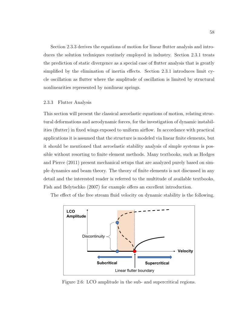
58

Section 2.3.3 derives the equations of motion for linear flutter analysis and intro-

duces the solution techniques routinely employed in industry. Section 2.3.1 treats

the prediction of static divergence as a special case of flutter analysis that is greatly

simplified by the elimination of inertia effects. Section 2.3.1 introduces limit cy-

cle oscillation as flutter where the amplitude of oscillation is limited by structural

nonlinearities represented by nonlinear springs.

2.3.3 Flutter Analysis

This section will present the classical aeroelastic equations of motion, relating struc-

tural deformations and aerodynamic forces, for the investigation of dynamic instabil-

ities (flutter) in fixed wings exposed to uniform airflow. In accordance with practical

applications it is assumed that the structure is modeled via linear finite elements, but

it should be mentioned that aeroelastic stability analysis of simple systems is pos-

sible without resorting to finite element methods. Many textbooks, such as Hodges

and Pierce (2011) present mechanical setups that are analyzed purely based on sim-

ple dynamics and beam theory. The theory of finite elements is not discussed in any

detail and the interested reader is referred to the multitude of available textbooks,

Fish and Belytschko (2007) for example offers an excellent introduction.

The effect of the free stream fluid velocity on dynamic stability is the following.

LCO Amplitude

Velocity

Subcritical Supercritical

Discontinuity

Linear flutter boundary

Figure 2.6: LCO amplitude in the sub- and supercritical regions.

59

At zero velocity the air has a minimal damping effect on structural deformation due

to the effort associated with the displacement of air. As the velocity increases the

damping effect generally increases initially, but if the velocity is increased further,

this trend is often reversed. For many structures a velocity threshold exists at

which the dampening effect of the airflow reverses. Beyond this flutter velocity

the aerodynamic forces feed oscillations which grow until structural failure occurs.

The general approach for determining the flutter velocity is to assume the existence

of steady harmonic oscillations of deformation at the flutter velocity. An iterative

process is employed to determine the fluid velocity and the oscillation that satisfy

the equation of motion.

State Space

In the finite element method the deformation of a flexible structure is represented by

the displacements of a finite set of locations (nodes). These nodes are connected by

elements representing relationships between the displacements based on geometry

and material properties. Assuming linear relationships between the stress and strain

in each element, and further assuming that the nodal displacements are small and

structural damping is negligible, the deformation of this discretized structure is

governed by the following equation of motion:

M ¨x(t) + Kx(t) = f(t) (2.49)

where x is the vector of time dependent nodal displacements and ¨x is its second time

derivative. The mass matrix M represents inertia effects, the stiffness matrix K

models the flexibility of the structure, and f represents the external forces applied

to the structure including aerodynamic forces.

The simpler steady state equation with constant displacement and applied forces

is given as:

Kxs = fs (2.50)

For the purpose of stability analysis the system is often linearized with respect to

60

the steady state solution xs via coordinate transformation:

x(t) = x(t)− xs (2.51)

Which leads to the following equation of motion in which fa represents the transient

aerodynamic forces caused by deformation from the steady state:

Mx(t) + Kx(t) = fa(x(t)) = f(t)− fs (2.52)

The notation fa(x(t)) indicates that the aerodynamic forces are a function not only

of the current displacements, but the complete history of displacements and could

be of the form: fa =∫. . .x(t)dt

Equation 2.52 is a closed-loop system and it is stable if any arbitrary small

deformation x0 converges to zero. It is possible to use Equation 2.52 directly, for

example by employing unsteady computational fluid dynamics (CFD) to obtain

the aerodynamic forces. Here the fluid velocity would be increased slowly while

simulating the system in a time-marching scheme until either the displacements

diverge or the maximum velocity of interest is reached. However this approach is

computationally very expensive and, therefore, the following sections will transform

the equation of motion to allow for more efficient methods of linear flutter analysis

commonly used in industry (Schuster et al. (2003)).

Modal Approach

A coordinate transformation Φ will express the displacements in terms of the eigen-

modes of the structure. The rationale of using this particular transformation is that

flutter is most often characterized by interactions of the first few modes, and using

as few as ten modes the flutter speed of a wing may be determined accurately (Zona

(2011)). In contrast, the number of structural nodes is often in the thousands, so

the transformation reduces the number of coordinates by orders of magnitude:

x(t) = Φq(t) (2.53)

with the generalized coordinates q(t). Each column of Φ is an eigenvector φi of

the structure, that is x(t) = φi sin(ωit) with eigenvalue ωi is a solution of the

61

homogeneous equation:

Mx(t) + Kx(t) = 0 (2.54)

Substitution and premultiplication with ΦT yields the transformed equation of mo-

tion:

ΦTMΦ q(t) + ΦTKΦ q(t) = ΦT fa(Φq(t)) (2.55)

Mq(t) +Kq(t) = fa(q(t)) (2.56)

where Equation 2.56 implicitly defines the transformed mass matrix M , stiffness

matrix K and aerodynamic forces fa as:

M = ΦTMΦ (2.57)

K = ΦTKΦ (2.58)

fa(q(t)) = ΦT fa(Φq(t)) (2.59)

Amplitude Linearization

A common assumption is that dynamic stability can be determined based on con-

vergence of infinitesimal displacements from the steady state. This is generally not

true in the case of limit cycle oscillations, but it leads to great simplifications for

flutter analysis. Based on the assumption of small displacements it is reason-

able to assume that the resulting aerodynamic forces are linear with respect to the

deformation:

fa(k1q1(t) + k2q2(t)) = k1fa(q1(t)) + k2fa(q2(t)) (2.60)

with constant factors k1 and k2. Further assuming a zero initial displacement com-

pletes the requirements of a continuous linear time-invariant system for which several

useful theorems are available. Specifically, the outputs (aerodynamic forces fa(t))

are related to the inputs (displacement x(t)) by the convolution integral:

fa(q(t)) =

∫ t

0

H(t− τ) q(t) dτ (2.61)

62

where H(t) is a matrix consisting of the (generally unknown) system’s response to

input pulses. However, it is more common to assume an impulse response that is

linear with respect to the free stream dynamic pressure q∞ and scale the argument

by the free stream velocity V divided by a reference length L, which is often defined

as half of the average chord length:

fa(q(t)) =

∫ t

0

q∞H

(V

L(t− τ)

)q(t) dτ (2.62)

Frequency Domain

In order to simplify the analysis, the problem is transferred to the frequency domain

via the Laplace transform defined as:

L{y(s)} =

∫ ∞0

e−sty(t) dt = y(s) (2.63)

where the unusual ˇ notation is chosen to maintain the convention that bold up-

percase letters denote matrices. Equation 2.62 is transformed using the convolution

theorem providing the Laplace transform of a convolution integral as:

L{∫ t

0

f(t)g(t− τ)dτ

}= L{f(t)}L {g(t)} (2.64)

This yields:

fa(s) = q∞ H

(V

Ls

)q(s) (2.65)

with H known as the aerodynamic transfer function that relates aerodynamic forces

to displacements in the Laplace domain.

Transformation of the Equation of motion 2.56 also requires the theorem appli-

cable to time differentials of signals with zero initial condition:

L{f(t)

}= s2L{f(t)} (2.66)

Now the Equation of motion 2.56 maybe transferred to the Laplace domain as:

Ms2q(s) +Kq(s) = q∞H

(L

Vs

)q(s) (2.67)

63

It is generally possible to obtain the aerodynamic transfer function H in the

s-domain to solve the equation of motion for q, which would then be transformed

back to the time domain via inverse Laplace transform. However it is much more

efficient to restrict solutions to the positive complex axis of the s-domain, which

corresponds to simple harmonic motion of the structure. This greatly simplifies

the calculation of the aerodynamic transfer function, but has the disadvantage that

the equation of motion 2.67 generally does not have such a solution. In fact, such

a harmonic solution only exists at certain velocities, the lowest positive of which

is defined as the flutter velocity. At all other velocities oscillations will either die

out (stable behavior) or grow exponentially (unstable). The corresponding equation

of motion is obtained by substituting iω for s, with ω being the frequency of the

harmonic oscillation:

− ω2Mq(iω) +Kq(iω) = q∞H

(L

Viω

)q(iω) (2.68)

This equation is commonly expressed using the reduced frequency k:

k =Lω

V(2.69)

(−ω2M +K − q∞H (ik)

)q(iω) = 0 (2.70)

Solution techniques for this equation are presented in Section 2.3.3 after a brief

discussion of modeling the unsteady aerodynamics.

Aerodynamic Models

Solving the flutter equation 2.70 requires a model of the aerodynamic forces that

act on the structure. This section will be restricted to a brief description of the

model used to obtain the aerodynamic forces in the subsonic model presented in the

results section. A concise overview of aerodynamic models relevant to aeroelastic

analysis is provided in many text books, for example chapter 3 of Rodden (2011).

The ZAERO theory manual (Zona (2011)) is also a very good reference, especially

with respect to numerical implementation.

64

In subsonic unsteady potential flow theory, it is assumed that the velocity field

is governed by a potential φ such that the components of the fluid velocity along

the x, y and z coordinates are given as:

u(x, y, z) = ∂φ(x,y,z)∂x

v(x, y, z) = ∂φ(x,y,z)∂y

w(x, y, z) = ∂φ(x,y,z)∂z

(2.71)

where u, v and w are the components of fluid velocity along the x, y and z co-

ordinates and ω(x, y, z) is the velocity potential. Given a steady stream of fluid

along the x-axis, the velocity potential around an obstacle (wing) is approximately

governed by

(1−M∞)φxx + φyy + φzz − 2M∞a∞

φxt −1

a2∞φtt = 0 (2.72)

where it is assumed that the disturbances from the steady flow are small. M∞ and

a∞ are respectively the Mach number and the speed of sound of the undisturbed

flow, and the indices denote partial derivatives. In the case where the movement of

the wing is given by a simple harmonic motion, the potential equation can be solved

numerically relatively efficiently in the Laplace domain. In general, the numerical

solution involves dividing the surface of the wing into small elements, each containing

one control point. At each control point the velocity potential is obtained, which

also yields the pressure on the surface based on the assumption of adiabatic flow:

p = p∞

(1− γ

a2∞(V∞φx + φt)

) γγ−1

(2.73)

where p∞ and V∞ denote the pressure and velocity of the undisturbed flow and γ

is the ratio of the specific heat at constant pressure to the specific heat at constant

volume of the fluid. The aerodynamic forces at the control points of the wing are

obtained by integration of the surface pressure. The equivalent generalized forces

on the structural model are provided by a spline model, which converts forces and

displacements between the structural finite element model and the aerodynamic

mesh.

65

Flutter Solution Methods

After deriving the equations of motion in the Laplace domain in Section 2.3.3,

the current Section discusses several solution techniques to determine the stability

boundary. To improve readability, the equation of motion in the Laplace domain

and the equation for harmonic motion, often referred to as the flutter equation, are

repeated here:

Ms2q(s) +Kq(s) = q∞H

(L

Vs

)q(s) (2.74)(

−ω2M +K − q∞H (ik))q(iω) = 0 (2.75)

The basic concept, shared by the following solution methods, is to modify the flutter

equation by adding a damping term so that it has solutions for all velocities. This

equation is then solved for a list of velocities and interpolated to obtain the solution

with zero added damping (if it exists).

The K-method, also referred to as the American method, introduces artificial

structural damping that is proportional to the stiffness as first proposed by Theodor-

son (1935): (−ω2M + (1 + igs)K − q∞H (ik)

)q(iω) = 0 (2.76)

where gs is a real number. The dynamic pressure q∞ is then expressed in terms of

the reduced frequency k (Equation 2.69) and fluid density ρ:

q∞ =1

2ρV 2∞ =

1

2ρ

(ωL

k

)2

(2.77)

and the resulting equation is divided by ω2 to obtain:(M +

ρ

2

(L

k

)2

H (ik) +1 + igsω2

K

)q = 0 (2.78)

A final substitution for the coefficient of K gives the final flutter equation for the

K-method:

λ =1 + igsω2

(2.79)

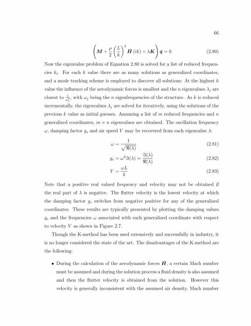
66

(M +

ρ

2

(L

k

)2

H (ik) + λK

)q = 0 (2.80)

Now the eigenvalue problem of Equation 2.80 is solved for a list of reduced frequen-

cies ki. For each k value there are as many solutions as generalized coordinates,

and a mode tracking scheme is employed to discover all solutions: At the highest k

value the influence of the aerodynamic forces is smallest and the n eigenvalues λj are

closest to 1ω2j, with ωj being the n eigenfrequencies of the structure. As k is reduced

incrementally, the eigenvalues λj are solved for iteratively, using the solutions of the

previous k value as initial guesses. Assuming a list of m reduced frequencies and n

generalized coordinates, m× n eigenvalues are obtained. The oscillation frequency

ω, damping factor gs and air speed V may be recovered from each eigenvalue λ:

ω =1√<(λ)

(2.81)

gs = ω2=(λ) ==(λ)

<(λ)(2.82)

V =ωL

k(2.83)

Note that a positive real valued frequency and velocity may not be obtained if

the real part of λ is negative. The flutter velocity is the lowest velocity at which

the damping factor gs switches from negative positive for any of the generalized

coordinates. These results are typically presented by plotting the damping values

gs and the frequencies ω associated with each generalized coordinate with respect

to velocity V as shown in Figure 2.7.

Though the K-method has been used extensively and successfully in industry, it

is no longer considered the state of the art. The disadvantages of the K-method are

the following:

• During the calculation of the aerodynamic forces H , a certain Mach number

must be assumed and during the solution process a fluid density is also assumed

and then the flutter velocity is obtained from the solution. However this

velocity is generally inconsistent with the assumed air density, Mach number

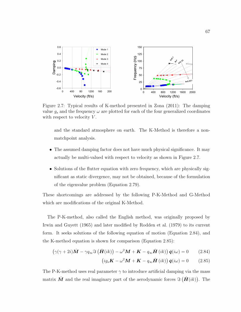
67

0

25

50

75

100

125

150

0 400 800 1200 1600 2000

Velocity (ft/s)

-0.6

-0.4

-0.2

0.0

0.2

0.4

0.6

0 400 80 1200 160 200

Mode 1

Mode 2

Mode 3

Mode 4

Velocity (ft/s)

Figure 2.7: Typical results of K-method presented in Zona (2011): The dampingvalue gs and the frequency ω are plotted for each of the four generalized coordinateswith respect to velocity V .

and the standard atmosphere on earth. The K-Method is therefore a non-

matchpoint analysis.

• The assumed damping factor does not have much physical significance. It may

actually be multi-valued with respect to velocity as shown in Figure 2.7.

• Solutions of the flutter equation with zero frequency, which are physically sig-

nificant as static divergence, may not be obtained, because of the formulation

of the eigenvalue problem (Equation 2.79).

These shortcomings are addressed by the following P-K-Method and G-Method

which are modifications of the original K-Method.

The P-K-method, also called the English method, was originally proposed by

Irwin and Guyett (1965) and later modified by Rodden et al. (1979) to its current

form. It seeks solutions of the following equation of motion (Equation 2.84), and

the K-method equation is shown for comparison (Equation 2.85):(γ(γ + 2i)M − γq∞=

(H(ik)

)− ω2M +K − q∞H (ik)

)q(iω) = 0 (2.84)(

igsK − ω2M +K − q∞H (ik))q(iω) = 0 (2.85)

The P-K-method uses real parameter γ to introduce artificial damping via the mass

matrix M and the real imaginary part of the aerodynamic forces =(H(ik)

). The

68

-0.6

-0.4

-0.2

0.0

0.2

0.4

0.6

600 700 800 900 1000 1100 1200 1300

Velocity (ft/s)

Mode 1

Mode 2

Mode 3

Mode 4

0.0

20.0

40.0

60.0

80.0

100.0

600 700 800 900 1000 1100 1200 1300

Velocity (ft/s)

Figure 2.8: Typical results of P-K-method presented in Zona (2011): The dampingvalue γ and the frequency ω are plotted for each of the four generalized coordinateswith respect to velocity V .

K-method, on the other hand, uses real parameter gs to introduce artificial damping

via the stiffness matrix. For given pairs of velocity V and fluid density ρ, Equation

2.84 is solved for γ and k via an iterative procedure. One such algorithm is detailed

in Rodden and Johnson (1994). Figure 2.8 shows the results of a flutter analysis

using the P-K-method for the same problem as in Figure 2.7.

Both the K-Method and the P-K-Method have been widely used in practice

and are discussed in virtually every textbook on aeroelasticity. The P-K-Method is

generally preferred and may be considered the standard for linear flutter analysis,

due to the following advantages:

• Equation 2.84 is solved for selected velocity/density pairs and the correspond-

ing Mach number is used the calculate the aerodynamic forces. This means the

analysis is a match point analysis, consistent with the standard atmosphere.

• The obtained damping values, for example in Figure 2.8, are generally per-

ceived to be more realistic and never multi-valued with respect to velocity.

• Because of it’s formulation, the P-K-method can obtain solutions with zero

frequency ω, corresponding to static divergence.

69

The G-Method (Chen (2000)) is another variation of the K-method that is imple-

mented in ZAERO Zona (2011). Its main advantage over the P-K-method is that

it generally provides a more realistic approximation of the damping coefficient. The

flutter equation is formulated in the s domain as:(V 2

L2p2M +K − 1

2ρV 2H (p)

)q(iω) = 0 (2.86)

p = g + ik = kγ + ik (2.87)

This is quite similar to the P-K-method equation, which may be written as:(V 2

L2p2M +K − 1

2ρV 2=

(H (ik)

)γ − 1

2ρV 2H (ik)

)q(iω) = 0 (2.88)

H is only available along the positive complex axis, therefore the G-method uses a

linear Taylor series:

H(p) ≈ H(ik) + g∂H(p)

∂g

∣∣∣∣g=0

(2.89)

The partial derivative may be transformed based on the Cauchy-Riemann equations,

such that only the function along the complex axis need to be known:

∂H(p)

∂g

∣∣∣∣g=0

=dH(ik)

d(ik)(2.90)

which can be approximated by numerical differentiation (finite differences).

Both the P-K-Method and the G-Method are well suited to predict both flutter

and static divergence instabilities and will determine the same maximum velocity.

However, one may argue that the G-method is more rigorously derived and provides

more realistic damping values over the whole velocity range. It has also been shown

that the G-method will detect bifurcations in the roots of the flutter equation, where

additional solutions (aerodynamic lag roots) appear at a certain velocities. Using

the P-K-method, these bifurcations may cause discontinuities in the damping values

with respect to the velocity, whereas the damping values obtained by the G-method

are continuous with respect the velocity (Zona (2011)).

70

Various software packages are available for the linear flutter analysis described

in this section, but large airspace companies often prefer their own proprietary

solutions due to better integration into their design process (Bhatia (2003)). Expe-

rienced engineers routinely perform linear flutter analysis with relative ease and it is

therefore considered a mature science (Schuster et al. (2003)). However, this gener-

ally involves manual selection of parameters affecting fidelity such as mesh density

and manual interpretation of results. Completely automated linear flutter analysis

still poses considerable challenges: For example even small changes in the natu-

ral frequencies can have unexpectedly large effects on the obtained flutter velocity,

which is generally linked to the interplay of different modes. As another example,

interpolation error in the calculation of aerodynamic forces may lead to “spurious”

roots of the flutter equation, causing underestimation of the flutter speed (Zona

(2011)).

2.3.4 Static Divergence

As described in Section 2.3.3, some flutter solution techniques are capable of pre-

dicting static divergence as well. However, if only the prediction of static divergence

is desired, then a much simpler static analysis is sufficient. This section describes

such analysis suitable for restrained cantilevered wings as proposed by Rodden and

Love (1985). Similar algorithms are implemented in virtually all commercial soft-

ware packages for aeroelastic analysis and extensively covered by textbooks such as

Rodden (2011) on which the following derivation is based.

Consider a thin cantilevered wing whose planform in the X-Y plane is represented

by a mesh of structural grid points. The airfoil, that is the shape of the cross-section

of the wing, is approximated by the Z-coordinates hi of the grid points. The airflow

along the X-axis is deflected by the wing and the resulting aerodynamic forces at

the grid points fa may be approximated by a linear equation:

fa =qS

cCah (2.91)

71

with dynamic pressure q, reference wing area S, reference chord length c and aerody-

namic influence coefficient matrix Ca. The aerodynamic influence coefficient matrix

Ca is obtained from numerical solution of the static velocity potential equation

(Section 2.3.3):

(1−M∞)φxx + φyy + φzz = 0 (2.92)

The fraction qSc

is merely a scaling factor and could be absorbed into the aerody-

namic influence coefficient matrix, but the representation above is more common

and it is important to realize that the aerodynamic forces are proportional to the

dynamic pressure, which is a quadratic function of the uniform velocity of the undis-

turbed air flow:

q =1

2ρv2 (2.93)

with air density ρ and velocity v. The deviation h from the X-Y plane is comprised

of two components

h = hr + hf (2.94)

where hr represents the known undeformed shape and hf corresponds to the flexible

deflection of the wing, which is related to the aerodynamic forces by the stiffness

matrix K:

Khf = fa (2.95)

Substitution of Equations 2.94 and 2.95 into Equation 2.91 relates the undeformed

shape hr to the flexible deformations hf :

Khf =qS

cCa(hr + hf ) (2.96)

which may be written as

(K − qS

cCa)hf =

qS

cCahr (2.97)

This equation may only be solved for the flexible deformation hf if the matrix on

the left hand side is nonsingular, therefore the following eigenvalue problem is of

special interest:

(K − qS

cCa)hf = 0 (2.98)

72

Negative values of dynamic pressure q that solve this equation have no physical

relevance, but positive solutions signify static divergence. If positive solutions exist,

Equation 2.93 may be solved for the lowest critical velocity at which divergence will

occur:

vd = 2ρ√q (2.99)

2.3.5 Limit Cycle Oscillations

As described in Section 2.3.1, limit cycle oscillations only occur in nonlinear systems.

Generally speaking, either aerodynamic or structural nonlinearities must be present.

For this reason, only a nonlinear model may predict LCO consistently. In many cases

numerical time integration of the state space model is employed to obtain the time

history for a given initial state and the presence of LCO must be judged from this

time history. For a single simulation this may be done manually by studying the

deformation history to detect sustained vibration. However, an automatic detection

algorithm is needed when larger numbers of samples are to be evaluated in the

context of numerical optimization or uncertainty quantification.

Detection of LCO based on mechanical energy

For the LCO test problem described in Section 4.1, the time response considered is

the mechanical energy defined as the sum of the kinetic and the strain energies. This

approach has the advantage of encompassing all the degrees of freedom of the system

in one quantity. For an asymptotically stable system, the energy will converge to the

steady state equilibrium characterized by constant zero kinetic energy and constant

potential energy. For a diverging system (static divergence or flutter) the system

energy will continue to grow unboundedly. In the case of LCO the mechanical

energy will hover consistently above the steady-state level and the kinetic energy will

oscillate periodically. Based on this criterion, design configurations may be classified

as stable or unstable and the method of support vector machines, described in the

following section, may be used to approximate the stability boundary.

73

2.4 Support Vector Machines (SVM)

This section will focus on a machine learning process, called support vector machine

(SVM), that is used throughout this work to approximate the boundaries between

feasible and infeasible regions of a parameterized design space. A review of the

theory behind SVM in Section 2.4.2 will be followed by a discussion of the advantages

and pitfalls in Section 2.4.3. It should be noted that SVM is a very popular approach

to the classification problem and a number of classic text books such as Alpaydin

(2004); Abe (2010); Scholkopf and Smola (2001) will provide a deeper understanding

than the following treatment.

2.4.1 Motivation

Many applications require the classification of samples into one or more classes.

Take for example the classification of emails into regular correspondence and spam.

Obviously an algorithm that will automatically sort out the spam mail is very useful,

but while it is easy for people to recognize unsolicited emails, the underlying “algo-

rithm” is not known and varies between users. What is known, however, is that the

decision is based on the content and origin of each message. The email classification

problem is therefore a popular application of machine learning algorithms that build

a classification function based on empirical data. Such an algorithm would analyze

a set of manually classified emails in order to categorize additional emails. Similar

problems exist in many areas of science, relating for example to the classification

of tissue samples, face recognition and of course, the classification of parameterized

designs as feasible or infeasible, which is the topic of this work.

2.4.2 Construction of SVM

The classification problem introduced above is formally defined as follows: Assume

an n-dimensional parameter space S ⊂ <n and a computable, deterministic classifier

c : S → {−1, 1} with binary output. Based on a set of training data: {xi, yi},i = 1, . . . , l, yi = c(xi), xi ∈ S predict the class (−1 or 1) of any additional

74

sample x ∈ S. In general, c may be stochastic, but this section will be limited to

the deterministic case, relevant to the deterministic simulation models presented in

Chapter 4.

Confusingly, the term SVM is generally used both for the predicting function

and for the machine learning process, which produces the predicting function. In

the first sense, the SVM is a scalar, analytical function s : S → < of the form

s(x) = b+l∑

i=1

λiyiK(xi,x) (2.100)

The training data is incorporated via the kernel function K and the SVM value is

a weighted sum with coefficients λi and offset b. Ideally, b and λi are selected such

that the sign of the SVM value predicts the class of any sample:

sgn(s(x)) ≈ c(x) (2.101)

and the most probable approximation of the boundary between the two domains is

the zero contour:

s(x) = 0 (2.102)

To describe the accuracy of the SVM, one distinguishes between the empirical

error (training error) and the true error of the SVM. The empirical error quantifies

the ability of the SVM to correctly classify the training samples and may be defined

as

εt =1

l

l∑i=1

fe(xi) with fe(x) =

1 if c(x) 6= sgn(s(x))

0 otherwise(2.103)

The simulation models presented in this dissertation are deterministic and with

proper selection of the kernel function (Section 2.4.2) the SVM will separate the

training samples. Therefore all SVMs discussed in Section 4 have zero training

error. The true error quantifies the ability of the SVM to correctly classify any

sample in the design space and is equivalent to the generalization error discussed

in Section 2.1.1. Only for very few analytical problems is it possible to calculate

the true error exactly. In the general case, the true error is approximated based

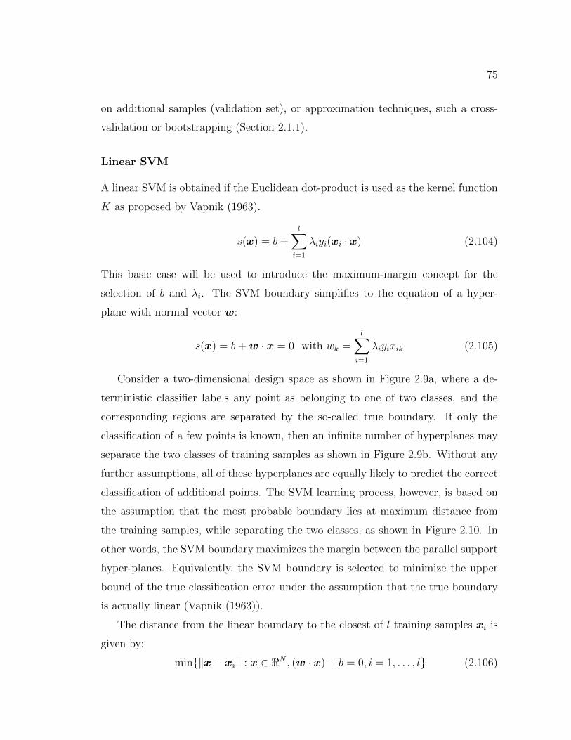
75

on additional samples (validation set), or approximation techniques, such a cross-

validation or bootstrapping (Section 2.1.1).

Linear SVM

A linear SVM is obtained if the Euclidean dot-product is used as the kernel function

K as proposed by Vapnik (1963).

s(x) = b+l∑

i=1

λiyi(xi · x) (2.104)

This basic case will be used to introduce the maximum-margin concept for the

selection of b and λi. The SVM boundary simplifies to the equation of a hyper-

plane with normal vector w:

s(x) = b+w · x = 0 with wk =l∑

i=1

λiyixik (2.105)

Consider a two-dimensional design space as shown in Figure 2.9a, where a de-

terministic classifier labels any point as belonging to one of two classes, and the

corresponding regions are separated by the so-called true boundary. If only the

classification of a few points is known, then an infinite number of hyperplanes may

separate the two classes of training samples as shown in Figure 2.9b. Without any

further assumptions, all of these hyperplanes are equally likely to predict the correct

classification of additional points. The SVM learning process, however, is based on

the assumption that the most probable boundary lies at maximum distance from

the training samples, while separating the two classes, as shown in Figure 2.10. In

other words, the SVM boundary maximizes the margin between the parallel support

hyper-planes. Equivalently, the SVM boundary is selected to minimize the upper

bound of the true classification error under the assumption that the true boundary

is actually linear (Vapnik (1963)).

The distance from the linear boundary to the closest of l training samples xi is

given by:

min{‖x− xi‖ : x ∈ <N , (w · x) + b = 0, i = 1, . . . , l} (2.106)

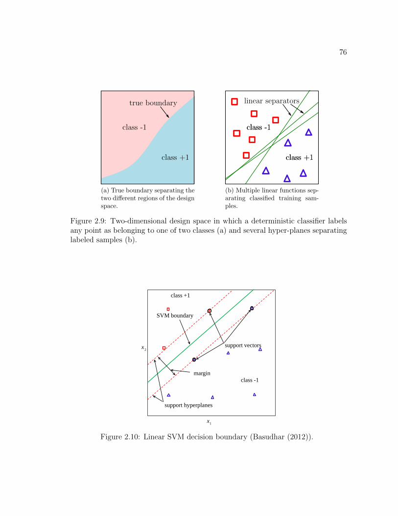
76

true boundary

class -1

class +1

(a) True boundary separating thetwo different regions of the designspace.

class -1

class +1

linear separators

class -1

class +1

(b) Multiple linear functions sep-arating classified training sam-ples.

Figure 2.9: Two-dimensional design space in which a deterministic classifier labelsany point as belonging to one of two classes (a) and several hyper-planes separatinglabeled samples (b).

class +1

SVM boundary

support vectors

margin

class -1

support hyperplanes

1x

2x

Figure 2.10: Linear SVM decision boundary (Basudhar (2012)).

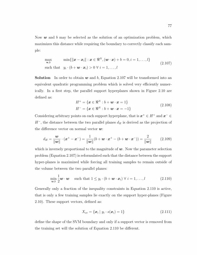
77

Now w and b may be selected as the solution of an optimization problem, which

maximizes this distance while requiring the boundary to correctly classify each sam-

ple:

maxw,b

min{‖x− xi‖ : x ∈ <N , (w · x) + b = 0, i = 1, . . . , l}

such that yi · (b+w · xi) > 0 ∀ i = 1, . . . , l(2.107)

Solution In order to obtain w and b, Equation 2.107 will be transformed into an

equivalent quadratic programming problem which is solved very efficiently numer-

ically. In a first step, the parallel support hyperplanes shown in Figure 2.10 are

defined as:

H+ = {x ∈ <N : b+w · x = 1}H− = {x ∈ <N : b+w · x = −1}

(2.108)

Considering arbitrary points on each support hyperplane, that is x+ ∈ H+ and x− ∈H−, the distance between the two parallel planes dH is derived as the projection of

the difference vector on normal vector w:

dH =w

‖w‖· (x+ − x−) =

1

‖w‖(b+w · x+ − (b+w · x−)) =

2

‖w‖(2.109)

which is inversely proportional to the magnitude of w. Now the parameter selection

problem (Equation 2.107) is reformulated such that the distance between the support

hyper-planes is maximized while forcing all training samples to remain outside of

the volume between the two parallel planes:

minw,b

1

2w ·w such that 1 ≤ yi · (b+w · xi) ∀ i = 1, . . . , l (2.110)

Generally only a fraction of the inequality constraints in Equation 2.110 is active,

that is only a few training samples lie exactly on the support hyper-planes (Figure

2.10). These support vectors, defined as:

Xsv = {xi | yi · s(xi) = 1} (2.111)

define the shape of the SVM boundary and only if a support vector is removed from

the training set will the solution of Equation 2.110 be different.

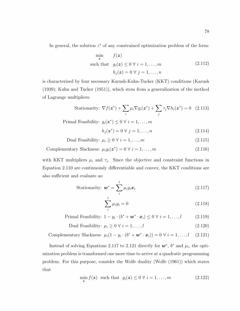
78

In general, the solution z∗ of any constrained optimization problem of the form:

minz

f(z)

such that gi(z) ≤ 0 ∀ i = 1, . . . ,m

hj(z) = 0 ∀ j = 1, . . . , n

(2.112)

is characterized by four necessary Karush-Kuhn-Tucker (KKT) conditions (Karush

(1939); Kuhn and Tucker (1951)), which stem from a generalization of the method

of Lagrange multipliers:

Stationarity: ∇f(z∗) +∑i

µi∇gi(z∗) +∑j

τj∇hi(z∗) = 0 (2.113)

Primal Feasibility: gi(z∗) ≤ 0 ∀ i = 1, . . . ,m

hj(z∗) = 0 ∀ j = 1, . . . , n (2.114)

Dual Feasibility: µi ≥ 0 ∀ i = 1, . . . ,m (2.115)

Complementary Slackness: µigi(z∗) = 0 ∀ i = 1, . . . ,m (2.116)

with KKT multipliers µi and τj. Since the objective and constraint functions in

Equation 2.110 are continuously differentiable and convex, the KKT conditions are

also sufficient and evaluate as:

Stationarity: w∗ =l∑i

µiyixi (2.117)

l∑i

µiyi = 0 (2.118)

Primal Feasibility: 1− yi · (b∗ +w∗ · xi) ≤ 0 ∀ i = 1, . . . , l (2.119)

Dual Feasibility: µi ≥ 0 ∀ i = 1, . . . , l (2.120)

Complementary Slackness: µi(1− yi · (b∗ +w∗ · xi)) = 0 ∀ i = 1, . . . , l (2.121)

Instead of solving Equations 2.117 to 2.121 directly for w∗, b∗ and µi, the opti-

mization problem is transformed one more time to arrive at a quadratic programming

problem. For this purpose, consider the Wolfe duality (Wolfe (1961)) which states

that

minzf(z) such that gi(z) ≤ 0 ∀ i = 1, . . . ,m (2.122)

79

has the same solution as its dual:

maxz,µ

f(z) +m∑i

µigi(z)

such that ∇f(z) +m∑i

µi∇gi(z) = 0

µi ≥ 0 ∀ i = 1, . . . , l (2.123)

if objective and constraint functions are continuously differentiable and convex. The

objective function of the Wolfe dual of Equation 2.110 may be expressed as:

1

2w∗ ·w∗ +

l∑i

µi (1− yi · (b∗ +w∗ · xi)) (2.124)

=1

2w∗ ·w∗ +

l∑i

µi − b∗l∑i

µiyi −w∗ ·l∑i

µiyixi

=l∑i

µi −l∑i,j

µiµjyiyj (xi · xj)

where w∗ and b∗ are eliminated by substituting the KKT conditions (Equations

2.117 and 2.118). The constraint function of the Wolfe dual is identical to the

stationarity KKT condition and simplifies to Equation 2.118. Finally, the Wolfe

dual may be expressed as a quadratic programming problem in terms of the vector

of multipliers µ:

maxµ

l∑i

µi −l∑i,j

µiµjyiyj (xi · xj)

such thatl∑i

µiyi = 0

µi ≥ 0 ∀ i = 1, . . . , l

(2.125)

Even for large sets of training data, Equation 2.125 can always be solved exactly

efficiently (Cristianini and Scholkopf (2002)), and an extensive review of solution

algorithms is given by Scholkopf et al. (1998). Once the solution µ∗ is known, w∗ is

provided by Equation 2.117 and b∗ is obtained by solving Equation 2.121 using any

80

non-zero multiplier µ∗k. Alternatively, the SVM itself is expressed in terms of the

multipliers µ∗ and offset b∗ by substitution of Equation 2.117 into Equation 2.105:

s(x) = b∗ +l∑i

µ∗i yi(xi · x) (2.126)

Nonlinear SVM

Of course in the general case, training samples may not be separable by a straight

hyper-plane. Fortunately, the SVM approach may be expanded to reproduce nonlin-

ear and disjoint boundaries via the so-called “kernel trick” (Aizerman et al. (1964)):

By replacing any dot products x ·y with a nonlinear scalar kernel function K(x,y),

as proposed by Boser et al. (1992), it is possible to obtain complex SVM boundaries

as shown in Figure 2.11, for example. This modification is equivalent to mapping the

training samples xi into a higher-dimensional feature space F , in which the samples

may be separated by a linear hyper-sphere. However, since both the SVM function

(Equation 2.126) and the quadratic programming problem (Equation 2.125) only

contain the kernel function (dot product), the transition from linear hyper-planes to

nonlinear SVM boundaries is rather small and does not actually require a mapping.

That is, the new quadratic programming problem and the SVM function are simply

given as:

maxµ

l∑i

µi −l∑i,j

µiµjyiyjK (xi,xj)

such thatl∑i

µiyi = 0

µi ≥ 0 ∀ i = 1, . . . , l

(2.127)

and

s(x) = b∗ +l∑i

µ∗i yiK(xi,x) (2.128)

where b∗ is obtained by solving the modified KKT complementary condition with

nonzero µ∗i :

µ∗i (1− yi · (b∗ +l∑j

µjyjK(xj,xi)) = 0 ∀ i = 1, . . . , l (2.129)

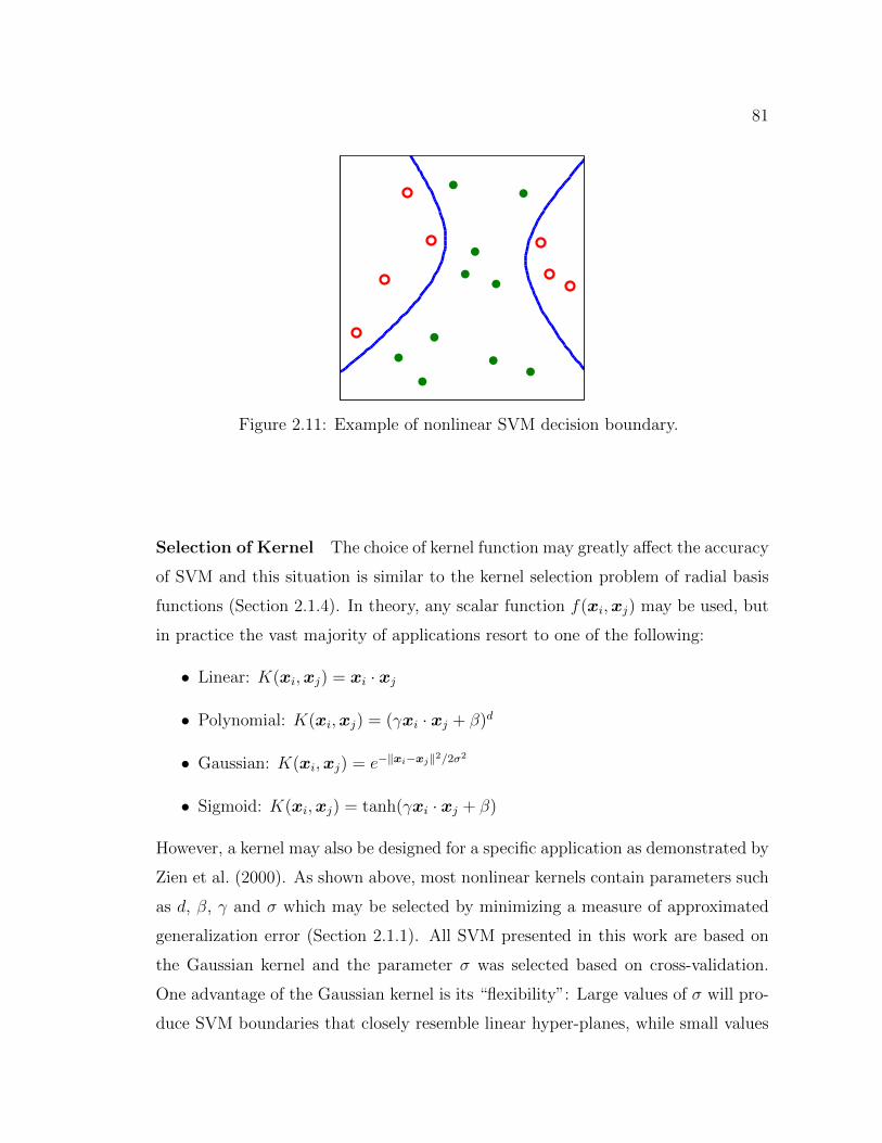
81

Figure 2.11: Example of nonlinear SVM decision boundary.

Selection of Kernel The choice of kernel function may greatly affect the accuracy

of SVM and this situation is similar to the kernel selection problem of radial basis

functions (Section 2.1.4). In theory, any scalar function f(xi,xj) may be used, but

in practice the vast majority of applications resort to one of the following:

• Linear: K(xi,xj) = xi · xj

• Polynomial: K(xi,xj) = (γxi · xj + β)d

• Gaussian: K(xi,xj) = e−‖xi−xj‖2/2σ2

• Sigmoid: K(xi,xj) = tanh(γxi · xj + β)

However, a kernel may also be designed for a specific application as demonstrated by

Zien et al. (2000). As shown above, most nonlinear kernels contain parameters such

as d, β, γ and σ which may be selected by minimizing a measure of approximated

generalization error (Section 2.1.1). All SVM presented in this work are based on

the Gaussian kernel and the parameter σ was selected based on cross-validation.

One advantage of the Gaussian kernel is its “flexibility”: Large values of σ will pro-

duce SVM boundaries that closely resemble linear hyper-planes, while small values

82

produce “more localized” boundaries as shown in Figure 2.11. Virtually any data

set becomes separable if a small enough σ is chosen. A more thorough discussion

of kernel functions is provided by many textbooks such as Alpaydin (2004); Abe

(2010); Scholkopf and Smola (2001). It should also be mentioned that the selection

of kernel parameters quickly becomes non-trivial if there are more than one or two

values to select. In this case, gradient-based optimization may be employed to min-

imize approximated generalization error as demonstrated by Chapelle et al. (2002)

on a kernel with more than 100 parameters.

As can be seen from Equation 2.100, an SVM, using one of the kernels above, is

a continuous analytical function s(x) for which the gradients with respect to x are

available analytically. This is relevant for applications in numerical optimization,

because it greatly improves the efficiency of gradient-based algorithms.

2.4.3 Discussion

Support vector machines have become a very popular tool for classification problems

and the hype around SVM has been compared to the popularity of neural networks

which they often replace. Successful applications include, for example, spam filter-

ing (Guzella and Caminhas (2009)), wind speed prediction (Mohandes et al. (2004)),

classification of cancer tissue (Furey et al. (2000)), recognition of handwritten dig-

its (Scholkopf et al. (1997)) and military vehicles (Karlsen et al. (2000)) and the

prediction of bankruptcy (Min and Lee (2005)). Because of the large number of pub-

lications, many review articles summarize the research for specific applications such

as chemistry (Li et al. (2009)), remote sensing (Mountrakis et al. (2011)), imaging

biomarkers (Orr et al. (2012)) or pattern recognition (Byun and Lee (2002)).

Advantages The general popularity of SVM may be attributed to the following

advantages: SVM routinely meet or exceed the prediction accuracy of other clas-

sification approaches such as neural networks and decision trees (Joachims (1998);

Bennett and Campbell (2000); Scholkopf et al. (1997)). This is in part due to the

flexibility of nonlinear kernels which allows for the reproduction of nonlinear, dis-

83

joint, boundaries. The SVM approach is well suited for high-dimensional training

samples, such as imaging data and large numbers of samples, found in extensive

databases. This often eliminates the need to carefully select features and training

samples. The methodology is easy to use and provides repeatable, consistent results.

Further simplification is due to the availability of sophisticated software packages,

such as Chang and Lin (2011), that solve the optimization problem (Equation 2.127)

and aid in the selection of kernel parameters.

Specifically for application in numerical design methods, SVM has the additional

advantage that the classifying function is analytical, differentiable and very cheap

to evaluate, which is important for gradient-based optimization and Monte-Carlo-

based uncertainty quantification. The training process is relatively quick as well,

thus enabling the use of adaptive sampling as described in Section 3.3.

Disadvantages It has been criticized that SVM do not “provide an explanation or

a comprehensible justification for the knowledge they learn” (Barakat and Bradley

(2010)). Lack of explanation can be a major obstacle to the acceptance of black-box

systems, for example in medical diagnosis and considerable research has therefore

been directed towards the extraction of rules from support vector machines as re-

viewed by Barakat and Bradley (2010).

Specifically for applications in numerical design methods, it has been noted that

SVM may require large numbers of samples to achieve the accuracy required for

numerical design methods (Basudhar et al. (2008)). This is a crucial issue if the

training data is not provided by an existing database, but instead requires expensive

simulations. To address this drawback, samples may be selected iteratively via adap-

tive sampling, where, based on a preliminary SVM boundary, additional training

samples are selected to refine the accuracy of the classifier. This approach, termed

explicit design space decomposition (EDSD) (Basudhar and Missoum (2010); Ba-

sudhar et al. (2012); Basudhar (2012)) was integrated into the algorithm proposed

in Chapter 3, that further incorporates lower-fidelity simulation models into the

learning process.

84

CHAPTER 3

MULTI-FIDELITY ALGORITHM

As stated in the introduction of this dissertation, design constraints characterized

by high cost of evaluating the corresponding simulation models and binary or dis-

continuous responses present a difficult obstacle to numerical optimization. Because

of the high cost of each evaluation, straight-forward optimization algorithms like ge-

netic programming are not feasible and more efficient algorithms based on surrogate

models and multi-fidelity methods are limited to continuous response models.

To address this challenge, this chapter proposes a multi-fidelity algorithm for the

construction of SVM representations of failure boundaries. The failure boundary,

also referred to as constraint boundary, is the boundary of the feasible region in the

design space. SVMs (Section 2.4) are widely used in computer science and their

advantages include the ability to approximate nonlinear, disjoint failure boundaries

in n-dimensional parameter spaces. Training samples are chosen iteratively, mini-

mizing simulation cost by carefully identifying points in the parameter space where

more information is needed. A key advantage of the algorithm and its main im-

provement over recent work by Basudhar and Missoum (2010) is the incorporation

of previous knowledge about the failure boundary to be approximated. That is, the

algorithm takes advantage of low-fidelity results to reduce the number of evaluations

of the high-fidelity model of interest.

This chapter is organized as follows: Section 3.1 analyzes and clarifies the as-

sumptions and goals that comprise the problem statement on which the development

of the algorithm is founded. The main concepts of the algorithm are outlined in

Section 3.2, followed by Section 3.3 which provides the level of detail required for

implementation. Finally, Section 3.4 applies the multi-fidelity algorithm to various

test problems to study its efficiency and convergence characteristics.

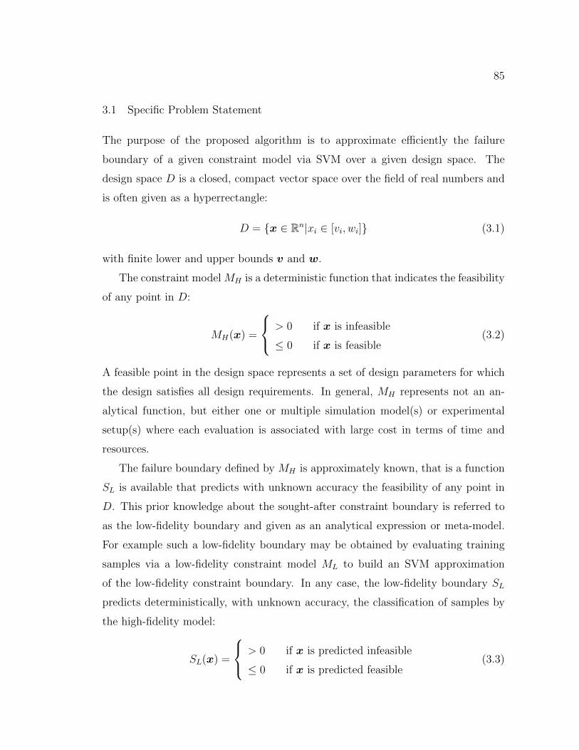
85

3.1 Specific Problem Statement

The purpose of the proposed algorithm is to approximate efficiently the failure

boundary of a given constraint model via SVM over a given design space. The

design space D is a closed, compact vector space over the field of real numbers and

is often given as a hyperrectangle:

D = {x ∈ Rn|xi ∈ [vi, wi]} (3.1)

with finite lower and upper bounds v and w.

The constraint model MH is a deterministic function that indicates the feasibility

of any point in D:

MH(x) =

> 0 if x is infeasible

≤ 0 if x is feasible(3.2)

A feasible point in the design space represents a set of design parameters for which

the design satisfies all design requirements. In general, MH represents not an an-

alytical function, but either one or multiple simulation model(s) or experimental

setup(s) where each evaluation is associated with large cost in terms of time and

resources.

The failure boundary defined by MH is approximately known, that is a function

SL is available that predicts with unknown accuracy the feasibility of any point in

D. This prior knowledge about the sought-after constraint boundary is referred to

as the low-fidelity boundary and given as an analytical expression or meta-model.

For example such a low-fidelity boundary may be obtained by evaluating training

samples via a low-fidelity constraint model ML to build an SVM approximation

of the low-fidelity constraint boundary. In any case, the low-fidelity boundary SL

predicts deterministically, with unknown accuracy, the classification of samples by

the high-fidelity model:

SL(x) =

> 0 if x is predicted infeasible

≤ 0 if x is predicted feasible(3.3)

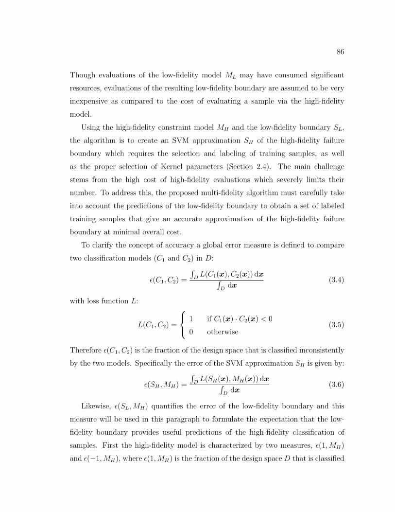
86

Though evaluations of the low-fidelity model ML may have consumed significant

resources, evaluations of the resulting low-fidelity boundary are assumed to be very

inexpensive as compared to the cost of evaluating a sample via the high-fidelity

model.

Using the high-fidelity constraint model MH and the low-fidelity boundary SL,

the algorithm is to create an SVM approximation SH of the high-fidelity failure

boundary which requires the selection and labeling of training samples, as well

as the proper selection of Kernel parameters (Section 2.4). The main challenge

stems from the high cost of high-fidelity evaluations which severely limits their

number. To address this, the proposed multi-fidelity algorithm must carefully take

into account the predictions of the low-fidelity boundary to obtain a set of labeled

training samples that give an accurate approximation of the high-fidelity failure

boundary at minimal overall cost.

To clarify the concept of accuracy a global error measure is defined to compare

two classification models (C1 and C2) in D:

ε(C1, C2) =

∫DL(C1(x), C2(x)) dx∫

Ddx

(3.4)

with loss function L:

L(C1, C2) =

1 if C1(x) · C2(x) < 0

0 otherwise(3.5)

Therefore ε(C1, C2) is the fraction of the design space that is classified inconsistently

by the two models. Specifically the error of the SVM approximation SH is given by:

ε(SH ,MH) =

∫DL(SH(x),MH(x)) dx∫

Ddx

(3.6)

Likewise, ε(SL,MH) quantifies the error of the low-fidelity boundary and this

measure will be used in this paragraph to formulate the expectation that the low-

fidelity boundary provides useful predictions of the high-fidelity classification of

samples. First the high-fidelity model is characterized by two measures, ε(1,MH)

and ε(−1,MH), where ε(1,MH) is the fraction of the design space D that is classified

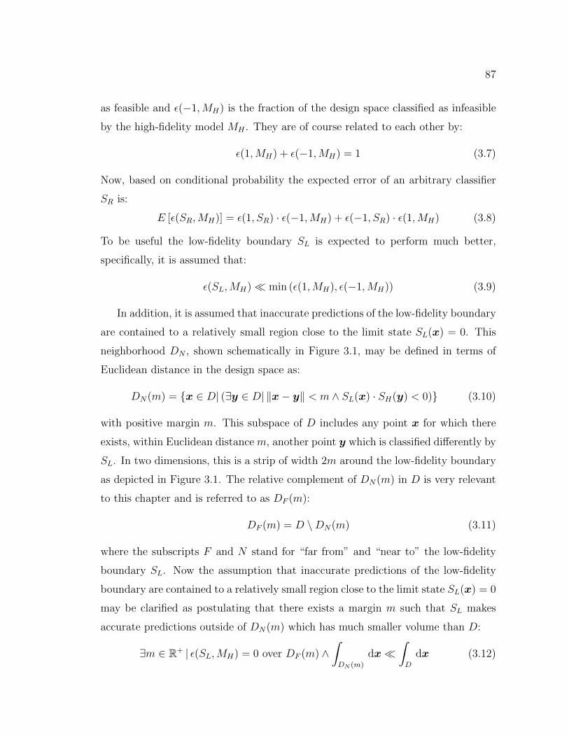
87

as feasible and ε(−1,MH) is the fraction of the design space classified as infeasible

by the high-fidelity model MH . They are of course related to each other by:

ε(1,MH) + ε(−1,MH) = 1 (3.7)

Now, based on conditional probability the expected error of an arbitrary classifier

SR is:

E [ε(SR,MH)] = ε(1, SR) · ε(−1,MH) + ε(−1, SR) · ε(1,MH) (3.8)

To be useful the low-fidelity boundary SL is expected to perform much better,

specifically, it is assumed that:

ε(SL,MH)� min (ε(1,MH), ε(−1,MH)) (3.9)

In addition, it is assumed that inaccurate predictions of the low-fidelity boundary

are contained to a relatively small region close to the limit state SL(x) = 0. This

neighborhood DN , shown schematically in Figure 3.1, may be defined in terms of

Euclidean distance in the design space as:

DN(m) = {x ∈ D| (∃y ∈ D| ‖x− y‖ < m ∧ SL(x) · SH(y) < 0)} (3.10)

with positive margin m. This subspace of D includes any point x for which there

exists, within Euclidean distance m, another point y which is classified differently by

SL. In two dimensions, this is a strip of width 2m around the low-fidelity boundary

as depicted in Figure 3.1. The relative complement of DN(m) in D is very relevant

to this chapter and is referred to as DF (m):

DF (m) = D \DN(m) (3.11)

where the subscripts F and N stand for “far from” and “near to” the low-fidelity

boundary SL. Now the assumption that inaccurate predictions of the low-fidelity

boundary are contained to a relatively small region close to the limit state SL(x) = 0

may be clarified as postulating that there exists a margin m such that SL makes

accurate predictions outside of DN(m) which has much smaller volume than D:

∃m ∈ R+ | ε(SL,MH) = 0 over DF (m) ∧∫DN (m)

dx�∫D

dx (3.12)

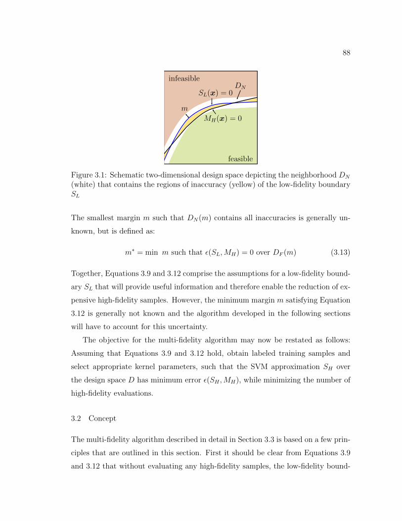
88

SL(x) = 0

m

MH(x) = 0

DN

infeasible

feasible

Figure 3.1: Schematic two-dimensional design space depicting the neighborhood DN

(white) that contains the regions of inaccuracy (yellow) of the low-fidelity boundarySL

The smallest margin m such that DN(m) contains all inaccuracies is generally un-

known, but is defined as:

m∗ = min m such that ε(SL,MH) = 0 over DF (m) (3.13)

Together, Equations 3.9 and 3.12 comprise the assumptions for a low-fidelity bound-

ary SL that will provide useful information and therefore enable the reduction of ex-

pensive high-fidelity samples. However, the minimum margin m satisfying Equation

3.12 is generally not known and the algorithm developed in the following sections

will have to account for this uncertainty.

The objective for the multi-fidelity algorithm may now be restated as follows:

Assuming that Equations 3.9 and 3.12 hold, obtain labeled training samples and

select appropriate kernel parameters, such that the SVM approximation SH over

the design space D has minimum error ε(SH ,MH), while minimizing the number of

high-fidelity evaluations.

3.2 Concept

The multi-fidelity algorithm described in detail in Section 3.3 is based on a few prin-

ciples that are outlined in this section. First it should be clear from Equations 3.9

and 3.12 that without evaluating any high-fidelity samples, the low-fidelity bound-

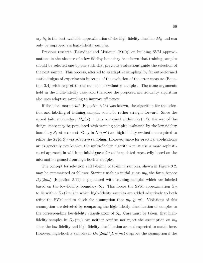
89

ary SL is the best available approximation of the high-fidelity classifier MH and can

only be improved via high-fidelity samples.

Previous research (Basudhar and Missoum (2010)) on building SVM approxi-

mations in the absence of a low-fidelity boundary has shown that training samples

should be selected one-by-one such that previous evaluations guide the selection of

the next sample. This process, referred to as adaptive sampling, by far outperformed

static designs of experiments in terms of the evolution of the error measure (Equa-

tion 3.4) with respect to the number of evaluated samples. The same arguments

hold in the multi-fidelity case, and therefore the proposed multi-fidelity algorithm

also uses adaptive sampling to improve efficiency.

If the ideal margin m∗ (Equation 3.13) was known, the algorithm for the selec-

tion and labeling of training samples could be rather straight forward: Since the

actual failure boundary MH(x) = 0 is contained within DN(m∗), the rest of the

design space may be populated with training samples evaluated by the low-fidelity

boundary SL at zero cost. Only in DN(m∗) are high-fidelity evaluations required to

refine the SVM SH via adaptive sampling. However, since for practical applications

m∗ is generally not known, the multi-fidelity algorithm must use a more sophisti-

cated approach in which an initial guess for m∗ is updated repeatedly based on the

information gained from high-fidelity samples.

The concept for selection and labeling of training samples, shown in Figure 3.2,

may be summarized as follows: Starting with an initial guess m0, the far subspace

DF (2m0) (Equation 3.11) is populated with training samples which are labeled

based on the low-fidelity boundary SL. This forces the SVM approximation SH

to lie within DN(2m0) in which high-fidelity samples are added adaptively to both

refine the SVM and to check the assumption that m0 ≥ m∗. Violations of this

assumption are detected by comparing the high-fidelity classification of samples to

the corresponding low-fidelity classification of SL. Care must be taken, that high-

fidelity samples in DN(m0) can neither confirm nor reject the assumption on m0

since the low-fidelity and high-fidelity classification are not expected to match here.

However, high-fidelity samples in DN(2m0)\DN(m0) disprove the assumption if the

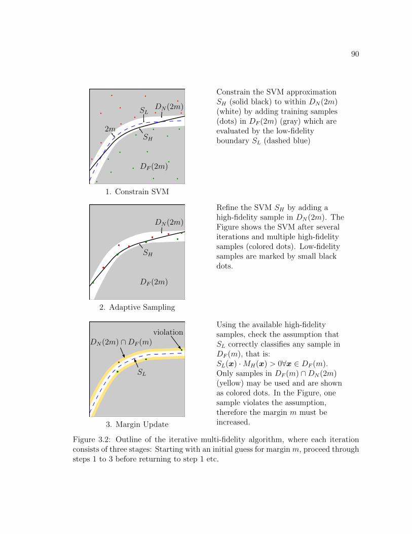
90

SL

2mSH

DF (2m)

DN(2m)

1. Constrain SVM

Constrain the SVM approximationSH (solid black) to within DN(2m)(white) by adding training samples(dots) in DF (2m) (gray) which areevaluated by the low-fidelityboundary SL (dashed blue)

SH

DF (2m)

DN(2m)

2. Adaptive Sampling

Refine the SVM SH by adding ahigh-fidelity sample in DN(2m). TheFigure shows the SVM after severaliterations and multiple high-fidelitysamples (colored dots). Low-fidelitysamples are marked by small blackdots.

DN(2m) ∩DF (m)

SL

violation

3. Margin Update

Using the available high-fidelitysamples, check the assumption thatSL correctly classifies any sample inDF (m), that is:SL(x) ·MH(x) > 0∀x ∈ DF (m).Only samples in DF (m) ∩DN(2m)(yellow) may be used and are shownas colored dots. In the Figure, onesample violates the assumption,therefore the margin m must beincreased.

Figure 3.2: Outline of the iterative multi-fidelity algorithm, where each iterationconsists of three stages: Starting with an initial guess for margin m, proceed throughsteps 1 to 3 before returning to step 1 etc.

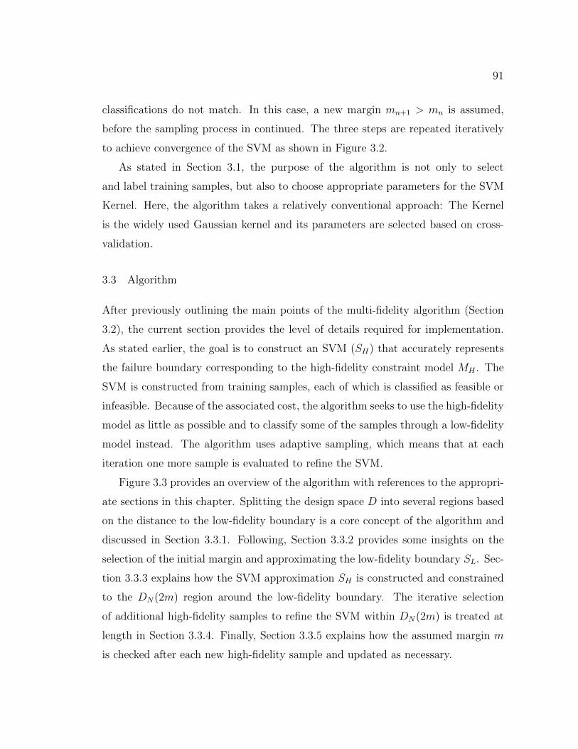
91

classifications do not match. In this case, a new margin mn+1 > mn is assumed,

before the sampling process in continued. The three steps are repeated iteratively

to achieve convergence of the SVM as shown in Figure 3.2.

As stated in Section 3.1, the purpose of the algorithm is not only to select

and label training samples, but also to choose appropriate parameters for the SVM

Kernel. Here, the algorithm takes a relatively conventional approach: The Kernel

is the widely used Gaussian kernel and its parameters are selected based on cross-

validation.

3.3 Algorithm

After previously outlining the main points of the multi-fidelity algorithm (Section

3.2), the current section provides the level of details required for implementation.

As stated earlier, the goal is to construct an SVM (SH) that accurately represents

the failure boundary corresponding to the high-fidelity constraint model MH . The

SVM is constructed from training samples, each of which is classified as feasible or

infeasible. Because of the associated cost, the algorithm seeks to use the high-fidelity

model as little as possible and to classify some of the samples through a low-fidelity

model instead. The algorithm uses adaptive sampling, which means that at each

iteration one more sample is evaluated to refine the SVM.

Figure 3.3 provides an overview of the algorithm with references to the appropri-

ate sections in this chapter. Splitting the design space D into several regions based

on the distance to the low-fidelity boundary is a core concept of the algorithm and

discussed in Section 3.3.1. Following, Section 3.3.2 provides some insights on the

selection of the initial margin and approximating the low-fidelity boundary SL. Sec-

tion 3.3.3 explains how the SVM approximation SH is constructed and constrained

to the DN(2m) region around the low-fidelity boundary. The iterative selection

of additional high-fidelity samples to refine the SVM within DN(2m) is treated at

length in Section 3.3.4. Finally, Section 3.3.5 explains how the assumed margin m

is checked after each new high-fidelity sample and updated as necessary.

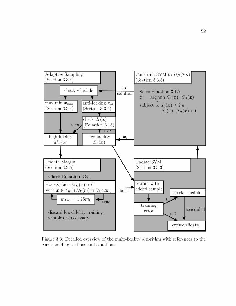
92

Update Margin(Section 3.3.5)

Update SVM(Section 3.3.3)

Adaptive Sampling(Section 3.3.4)

Check Equation 3.33:

cross-validate

check schedule

Solve Equation 3.17:xc = arg min

xSL(x) · SH(x)

subject to dL(x) ≥ 2mSL(x) · SH(x) < 0

check schedule

> m

< m

0

> 0scheduled

Constrain SVM to DN(2m)(Section 3.3.3)

xc

nosolution

max-min xmm(Section 3.3.4)

anti-locking xal(Section 3.3.4)

check dL(x)(Equation 3.15)

high-fidelityMH(x)

low-fidelitySL(x)

mk+1 = 1.25mk

∃x : SL(x) ·MH(x) < 0with x ∈ TH ∩DF (m) ∩DN(2m) false

true

retrain withadded sample

trainingerrordiscard low-fidelity training

samples as necessary

Figure 3.3: Detailed overview of the multi-fidelity algorithm with references to thecorresponding sections and equations.

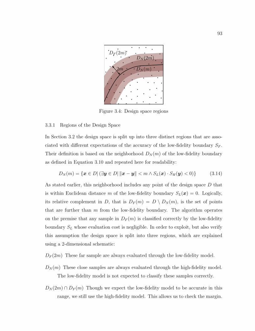
93

DN(2m)

DN(m)

DF (2m)

2m

Figure 3.4: Design space regions

3.3.1 Regions of the Design Space

In Section 3.2 the design space is split up into three distinct regions that are asso-

ciated with different expectations of the accuracy of the low-fidelity boundary SF .

Their definition is based on the neighborhood DN(m) of the low-fidelity boundary

as defined in Equation 3.10 and repeated here for readability:

DN(m) = {x ∈ D| (∃y ∈ D| ‖x− y‖ < m ∧ SL(x) · SH(y) < 0)} (3.14)

As stated earlier, this neighborhood includes any point of the design space D that

is within Euclidean distance m of the low-fidelity boundary SL(x) = 0. Logically,

its relative complement in D, that is DF (m) = D \ DN(m), is the set of points

that are further than m from the low-fidelity boundary. The algorithm operates

on the premise that any sample in DF (m) is classified correctly by the low-fidelity

boundary SL whose evaluation cost is negligible. In order to exploit, but also verify

this assumption the design space is split into three regions, which are explained

using a 2-dimensional schematic:

DF (2m) These far sample are always evaluated through the low-fidelity model.

DN(m) These close samples are always evaluated through the high-fidelity model.

The low-fidelity model is not expected to classify these samples correctly.

DN(2m) ∩DF (m) Though we expect the low-fidelity model to be accurate in this

range, we still use the high-fidelity model. This allows us to check the margin.

94

If samples in this region are misclassified by the low-fidelity model the margin

is increased.

Clearly, the algorithm must be able to determine which region a point x belongs

to, which requires the Euclidean distance to the low-fidelity boundary. This dis-

tance dL(x) may be obtained by solving the following optimization problem which

seeks the closest other point y ∈ D that is classified differently by the low-fidelity

boundary SL:

dL(x) = miny‖x− y‖ subject to: SL(x) · SL(y) < 0 (3.15)

Solving this optimization problem efficiently is non-trivial due to the likelihood

of multiple local optima. The current implementation uses a Monte-Carlo search

to find a good initial guess which is then refined via gradient-based optimization

(SQP) with analytical gradients. As detailed in the following Sections, the multi-

fidelity algorithm may require this distance for large numbers of points, which can

be addressed by building a Kriging model of dL(x). This is efficient because the

required accuracy is not very high and the low-fidelity boundary SL is fixed, which

means the Kriging model must be built only once. The practical implementation

of the algorithm uses dL to determine which region a point x belongs to via the

following equivalences:

dL(x) < m ≡ x ∈ DN(m)

dL(x) ≥ 2m ≡ x ∈ DF (2m)

m < dL(x) < 2m ≡ x ∈ DN(2m) ∩DF (m)

(3.16)

3.3.2 Initial Setup

Starting the multi-fidelity algorithm requires a high-fidelity constraint model MH ,

a low-fidelity boundary SL and an initial guess for the margin m. While MH is

considered a given, the other two invite further explanaition. First, however, to

avoid any confusion, the distinction between the 4 classifiers introduced in Section

3.1 is summarized:

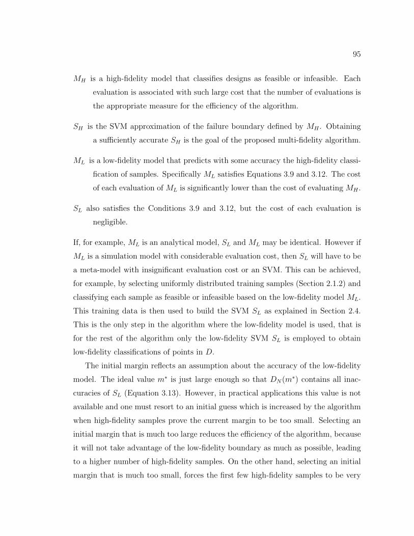
95

MH is a high-fidelity model that classifies designs as feasible or infeasible. Each

evaluation is associated with such large cost that the number of evaluations is

the appropriate measure for the efficiency of the algorithm.

SH is the SVM approximation of the failure boundary defined by MH . Obtaining

a sufficiently accurate SH is the goal of the proposed multi-fidelity algorithm.

ML is a low-fidelity model that predicts with some accuracy the high-fidelity classi-

fication of samples. Specifically ML satisfies Equations 3.9 and 3.12. The cost

of each evaluation of ML is significantly lower than the cost of evaluating MH .

SL also satisfies the Conditions 3.9 and 3.12, but the cost of each evaluation is

negligible.

If, for example, ML is an analytical model, SL and ML may be identical. However if

ML is a simulation model with considerable evaluation cost, then SL will have to be

a meta-model with insignificant evaluation cost or an SVM. This can be achieved,

for example, by selecting uniformly distributed training samples (Section 2.1.2) and

classifying each sample as feasible or infeasible based on the low-fidelity model ML.

This training data is then used to build the SVM SL as explained in Section 2.4.

This is the only step in the algorithm where the low-fidelity model is used, that is

for the rest of the algorithm only the low-fidelity SVM SL is employed to obtain

low-fidelity classifications of points in D.

The initial margin reflects an assumption about the accuracy of the low-fidelity

model. The ideal value m∗ is just large enough so that DN(m∗) contains all inac-

curacies of SL (Equation 3.13). However, in practical applications this value is not

available and one must resort to an initial guess which is increased by the algorithm

when high-fidelity samples prove the current margin to be too small. Selecting an

initial margin that is much too large reduces the efficiency of the algorithm, because

it will not take advantage of the low-fidelity boundary as much as possible, leading

to a higher number of high-fidelity samples. On the other hand, selecting an initial

margin that is much too small, forces the first few high-fidelity samples to be very

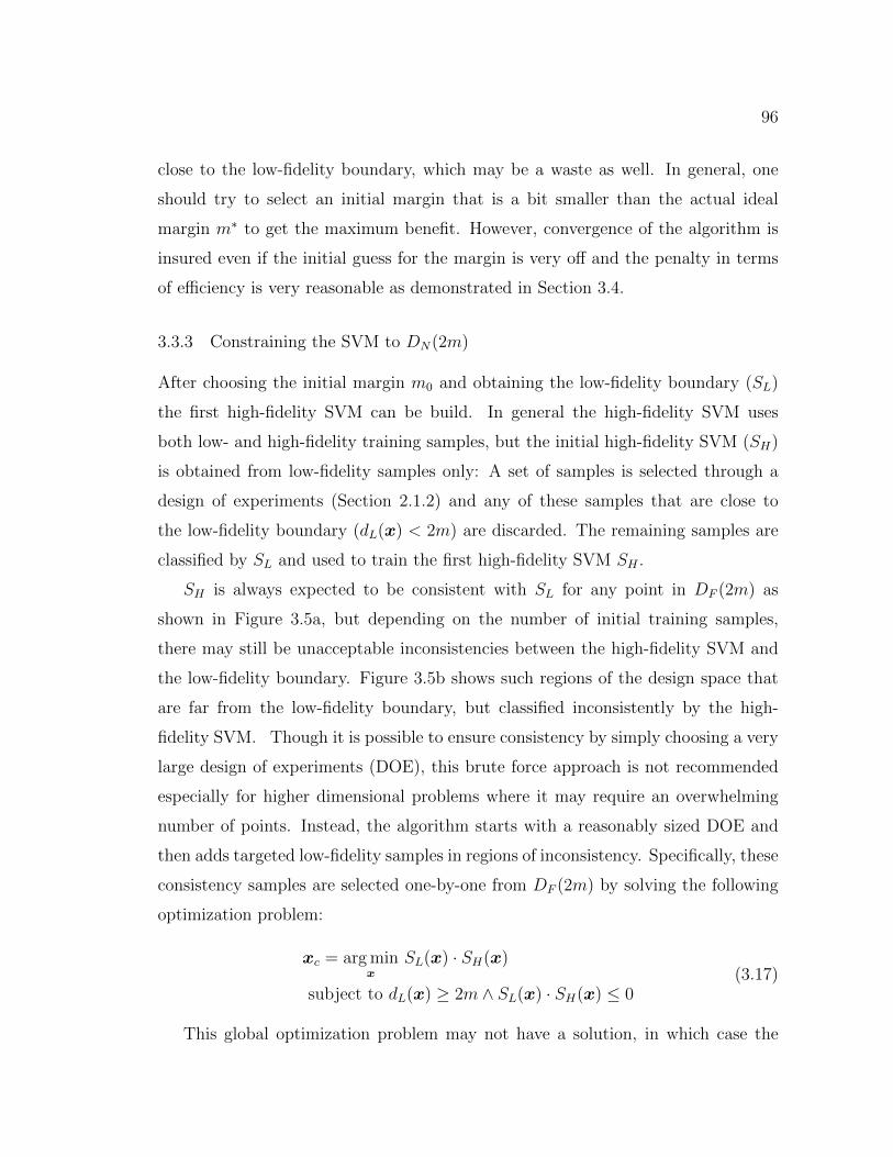
96

close to the low-fidelity boundary, which may be a waste as well. In general, one

should try to select an initial margin that is a bit smaller than the actual ideal

margin m∗ to get the maximum benefit. However, convergence of the algorithm is

insured even if the initial guess for the margin is very off and the penalty in terms

of efficiency is very reasonable as demonstrated in Section 3.4.

3.3.3 Constraining the SVM to DN(2m)

After choosing the initial margin m0 and obtaining the low-fidelity boundary (SL)

the first high-fidelity SVM can be build. In general the high-fidelity SVM uses

both low- and high-fidelity training samples, but the initial high-fidelity SVM (SH)

is obtained from low-fidelity samples only: A set of samples is selected through a

design of experiments (Section 2.1.2) and any of these samples that are close to

the low-fidelity boundary (dL(x) < 2m) are discarded. The remaining samples are

classified by SL and used to train the first high-fidelity SVM SH .

SH is always expected to be consistent with SL for any point in DF (2m) as

shown in Figure 3.5a, but depending on the number of initial training samples,

there may still be unacceptable inconsistencies between the high-fidelity SVM and

the low-fidelity boundary. Figure 3.5b shows such regions of the design space that

are far from the low-fidelity boundary, but classified inconsistently by the high-

fidelity SVM. Though it is possible to ensure consistency by simply choosing a very

large design of experiments (DOE), this brute force approach is not recommended

especially for higher dimensional problems where it may require an overwhelming

number of points. Instead, the algorithm starts with a reasonably sized DOE and

then adds targeted low-fidelity samples in regions of inconsistency. Specifically, these

consistency samples are selected one-by-one from DF (2m) by solving the following

optimization problem:

xc = arg minx

SL(x) · SH(x)

subject to dL(x) ≥ 2m ∧ SL(x) · SH(x) ≤ 0(3.17)

This global optimization problem may not have a solution, in which case the

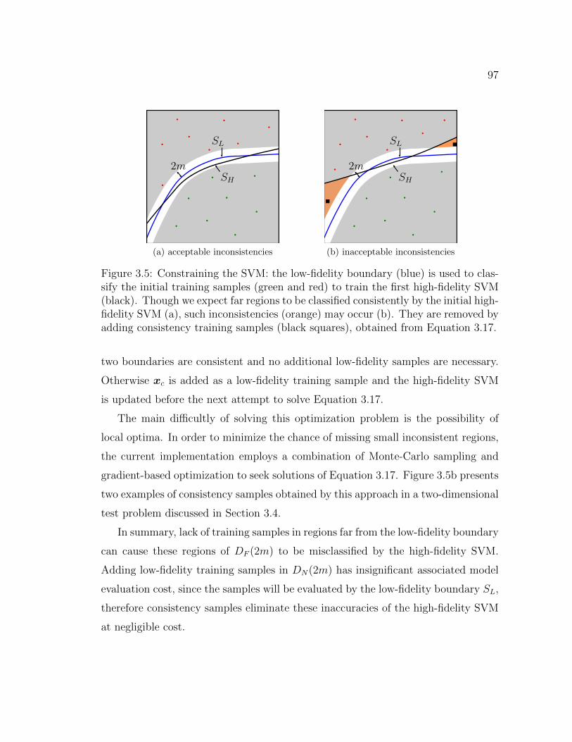
97

SL

2mSH

(a) acceptable inconsistencies

SL

2mSH

(b) inacceptable inconsistencies

Figure 3.5: Constraining the SVM: the low-fidelity boundary (blue) is used to clas-sify the initial training samples (green and red) to train the first high-fidelity SVM(black). Though we expect far regions to be classified consistently by the initial high-fidelity SVM (a), such inconsistencies (orange) may occur (b). They are removed byadding consistency training samples (black squares), obtained from Equation 3.17.

two boundaries are consistent and no additional low-fidelity samples are necessary.

Otherwise xc is added as a low-fidelity training sample and the high-fidelity SVM

is updated before the next attempt to solve Equation 3.17.

The main difficultly of solving this optimization problem is the possibility of

local optima. In order to minimize the chance of missing small inconsistent regions,

the current implementation employs a combination of Monte-Carlo sampling and

gradient-based optimization to seek solutions of Equation 3.17. Figure 3.5b presents

two examples of consistency samples obtained by this approach in a two-dimensional

test problem discussed in Section 3.4.

In summary, lack of training samples in regions far from the low-fidelity boundary

can cause these regions of DF (2m) to be misclassified by the high-fidelity SVM.

Adding low-fidelity training samples in DN(2m) has insignificant associated model

evaluation cost, since the samples will be evaluated by the low-fidelity boundary SL,

therefore consistency samples eliminate these inaccuracies of the high-fidelity SVM

at negligible cost.

98

Construction of Support Vector Machine

In addition to a set of classified training samples, constructing the SVM also requires

the selection of a Kernel function and corresponding Kernel parameters as discussed

in Section 2.4. The current algorithm uses the general-purpose Gaussian kernel:

K(xi,xj) = e−‖xi−xj‖2/2σ2

(3.18)

with parameter σ to obtain a nonlinear SVM boundary. σ is selected from a discrete

set of logarithmically spaced values to minimize the cross-validation error (Section

2.1.1). Since the multi-fidelity algorithm is geared towards deterministic constraint

models, the training samples are expected to be separable and no training error is

permitted (Section 2.4.2). This is achieved by ignoring all values of σ that result in

non-zero training error, regardless of the corresponding cross-validation error.

3.3.4 Adaptive Sampling

After the high-fidelity SVM has been constrained to the DN(2m) neighborhood of

the low-fidelity boundary SL as described in the previous Section 3.3.3, the next

step is to add a high-fidelity sample to refine SH in DN(2m). The current section

will first discuss the selection of these samples in general terms before presenting

the finer details in Sections 3.3.4 and 3.3.4. The concept of adaptive sampling is

to use the current SVM and its distribution of training samples to predict where

additional information in the form of an evaluated sample will be most helpful to

improve the SVM.

The selection of these samples as part of the multi-fidelity algorithm is based on

two algorithms developed by Anirban Basudhar as part of his dissertation research

(Basudhar (2012)). Specifically the max-min samples described below are identical

to the primary samples proposed in Basudhar and Missoum (2010). Likewise, the

anti-locking samples (Section 3.3.4) are similar to, and serve the same purpose as

the secondary samples proposed in Basudhar and Missoum (2010).

The underlying idea for the max-min samples is that adding a sample right on

the SVM boundary SH(x) = 0 is guaranteed to modify the SVM. Further, the

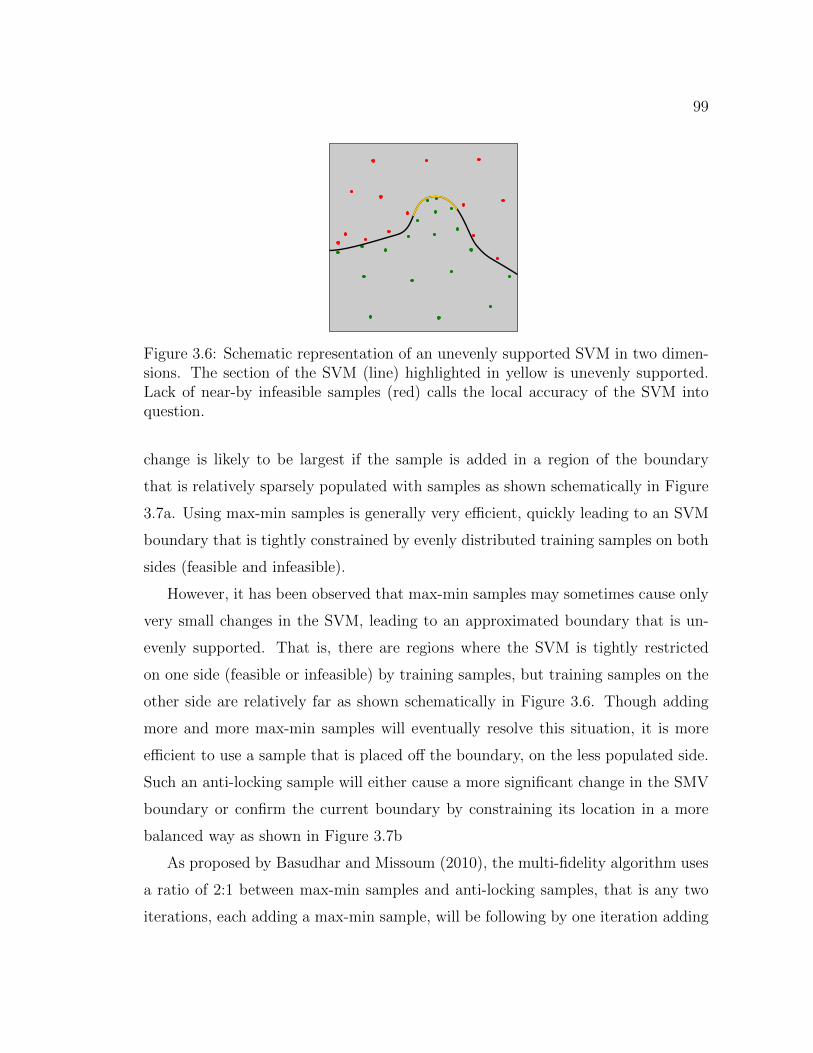
99

Figure 3.6: Schematic representation of an unevenly supported SVM in two dimen-sions. The section of the SVM (line) highlighted in yellow is unevenly supported.Lack of near-by infeasible samples (red) calls the local accuracy of the SVM intoquestion.

change is likely to be largest if the sample is added in a region of the boundary

that is relatively sparsely populated with samples as shown schematically in Figure

3.7a. Using max-min samples is generally very efficient, quickly leading to an SVM

boundary that is tightly constrained by evenly distributed training samples on both

sides (feasible and infeasible).

However, it has been observed that max-min samples may sometimes cause only

very small changes in the SVM, leading to an approximated boundary that is un-

evenly supported. That is, there are regions where the SVM is tightly restricted

on one side (feasible or infeasible) by training samples, but training samples on the

other side are relatively far as shown schematically in Figure 3.6. Though adding

more and more max-min samples will eventually resolve this situation, it is more

efficient to use a sample that is placed off the boundary, on the less populated side.

Such an anti-locking sample will either cause a more significant change in the SMV

boundary or confirm the current boundary by constraining its location in a more

balanced way as shown in Figure 3.7b

As proposed by Basudhar and Missoum (2010), the multi-fidelity algorithm uses

a ratio of 2:1 between max-min samples and anti-locking samples, that is any two

iterations, each adding a max-min sample, will be following by one iteration adding

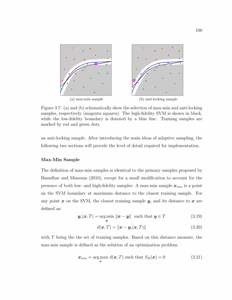
100

(a) max-min sample (b) anti-locking sample

Figure 3.7: (a) and (b) schematically show the selection of max-min and anti-lockingsamples, respectively (magenta squares). The high-fidelity SVM is shown in black,while the low-fidelity boundary is denoted by a blue line. Training samples aremarked by red and green dots.

an anti-locking sample. After introducing the main ideas of adaptive sampling, the

following two sections will provide the level of detail required for implementation.

Max-Min Sample

The definition of max-min samples is identical to the primary samples proposed by

Basudhar and Missoum (2010), except for a small modification to account for the

presence of both low- and high-fidelity samples. A max-min sample xmm is a point

on the SVM boundary at maximum distance to the closest training sample. For

any point x on the SVM, the closest training sample yc and its distance to x are

defined as:

yc(x, T ) = arg miny

‖x− y‖ such that y ∈ T (3.19)

d(x, T ) = ‖x− yc(x, T )‖ (3.20)

with T being the the set of training samples. Based on this distance measure, the

max-min sample is defined as the solution of an optimization problem:

xmm = arg maxx

d(x, T ) such that SH(x) = 0 (3.21)

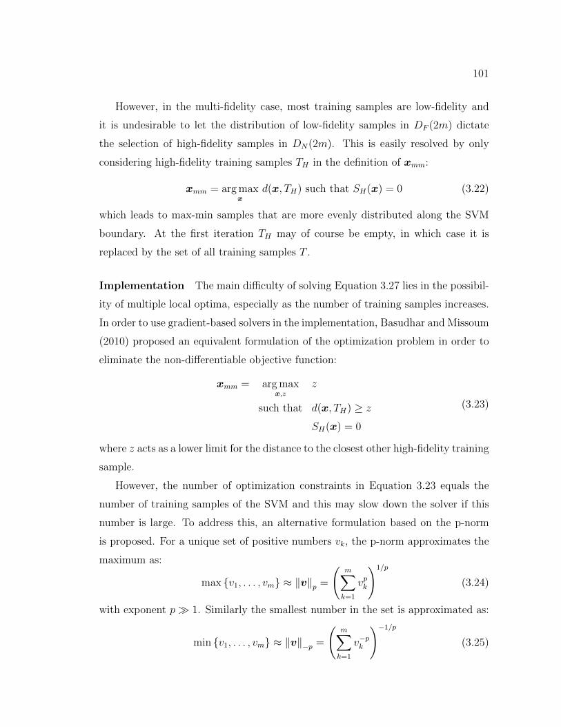
101

However, in the multi-fidelity case, most training samples are low-fidelity and

it is undesirable to let the distribution of low-fidelity samples in DF (2m) dictate

the selection of high-fidelity samples in DN(2m). This is easily resolved by only

considering high-fidelity training samples TH in the definition of xmm:

xmm = arg maxx

d(x, TH) such that SH(x) = 0 (3.22)

which leads to max-min samples that are more evenly distributed along the SVM

boundary. At the first iteration TH may of course be empty, in which case it is

replaced by the set of all training samples T .

Implementation The main difficulty of solving Equation 3.27 lies in the possibil-

ity of multiple local optima, especially as the number of training samples increases.

In order to use gradient-based solvers in the implementation, Basudhar and Missoum

(2010) proposed an equivalent formulation of the optimization problem in order to

eliminate the non-differentiable objective function:

xmm = arg maxx,z

z

such that d(x, TH) ≥ z

SH(x) = 0

(3.23)

where z acts as a lower limit for the distance to the closest other high-fidelity training

sample.

However, the number of optimization constraints in Equation 3.23 equals the

number of training samples of the SVM and this may slow down the solver if this

number is large. To address this, an alternative formulation based on the p-norm

is proposed. For a unique set of positive numbers vk, the p-norm approximates the

maximum as:

max {v1, . . . , vm} ≈ ‖v‖p =

(m∑k=1

vpk

)1/p

(3.24)

with exponent p� 1. Similarly the smallest number in the set is approximated as:

min {v1, . . . , vm} ≈ ‖v‖−p =

(m∑k=1

v−pk

)−1/p(3.25)

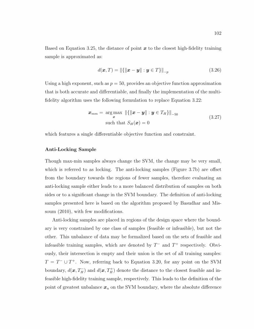
102

Based on Equation 3.25, the distance of point x to the closest high-fidelity training

sample is approximated as:

d(x, T ) = ‖{‖x− y‖ : y ∈ T}‖−p (3.26)

Using a high exponent, such as p = 50, provides an objective function approximation

that is both accurate and differentiable, and finally the implementation of the multi-

fidelity algorithm uses the following formulation to replace Equation 3.22:

xmm = arg maxx

‖{‖x− y‖ : y ∈ TH}‖−50

such that SH(x) = 0(3.27)

which features a single differentiable objective function and constraint.

Anti-Locking Sample

Though max-min samples always change the SVM, the change may be very small,

which is referred to as locking. The anti-locking samples (Figure 3.7b) are offset

from the boundary towards the regions of fewer samples, therefore evaluating an

anti-locking sample either leads to a more balanced distribution of samples on both

sides or to a significant change in the SVM boundary. The definition of anti-locking

samples presented here is based on the algorithm proposed by Basudhar and Mis-

soum (2010), with few modifications.

Anti-locking samples are placed in regions of the design space where the bound-

ary is very constrained by one class of samples (feasible or infeasible), but not the

other. This unbalance of data may be formalized based on the sets of feasible and

infeasible training samples, which are denoted by T− and T+ respectively. Obvi-

ously, their intersection is empty and their union is the set of all training samples:

T = T− ∪ T+. Now, referring back to Equation 3.20, for any point on the SVM

boundary, d(x, T−H ) and d(x, T+H ) denote the distance to the closest feasible and in-

feasible high-fidelity training sample, respectively. This leads to the definition of the

point of greatest unbalance xu on the SVM boundary, where the absolute difference

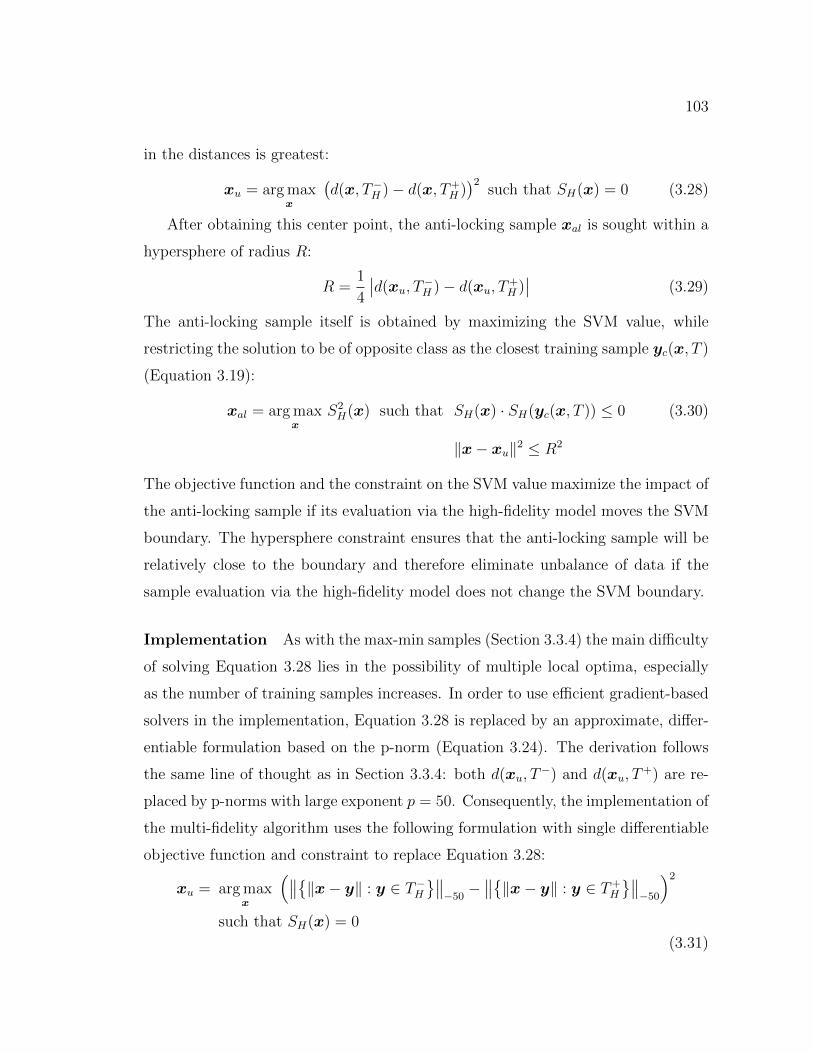
103

in the distances is greatest:

xu = arg maxx

(d(x, T−H )− d(x, T+

H ))2

such that SH(x) = 0 (3.28)

After obtaining this center point, the anti-locking sample xal is sought within a

hypersphere of radius R:

R =1

4

∣∣d(xu, T−H )− d(xu, T

+H )∣∣ (3.29)

The anti-locking sample itself is obtained by maximizing the SVM value, while

restricting the solution to be of opposite class as the closest training sample yc(x, T )

(Equation 3.19):

xal = arg maxx

S2H(x) such that SH(x) · SH(yc(x, T )) ≤ 0 (3.30)

‖x− xu‖2 ≤ R2

The objective function and the constraint on the SVM value maximize the impact of

the anti-locking sample if its evaluation via the high-fidelity model moves the SVM

boundary. The hypersphere constraint ensures that the anti-locking sample will be

relatively close to the boundary and therefore eliminate unbalance of data if the

sample evaluation via the high-fidelity model does not change the SVM boundary.

Implementation As with the max-min samples (Section 3.3.4) the main difficulty

of solving Equation 3.28 lies in the possibility of multiple local optima, especially

as the number of training samples increases. In order to use efficient gradient-based

solvers in the implementation, Equation 3.28 is replaced by an approximate, differ-

entiable formulation based on the p-norm (Equation 3.24). The derivation follows

the same line of thought as in Section 3.3.4: both d(xu, T−) and d(xu, T

+) are re-

placed by p-norms with large exponent p = 50. Consequently, the implementation of

the multi-fidelity algorithm uses the following formulation with single differentiable

objective function and constraint to replace Equation 3.28:

xu = arg maxx

(∥∥{‖x− y‖ : y ∈ T−H}∥∥−50 −

∥∥{‖x− y‖ : y ∈ T+H

}∥∥−50

)2such that SH(x) = 0

(3.31)

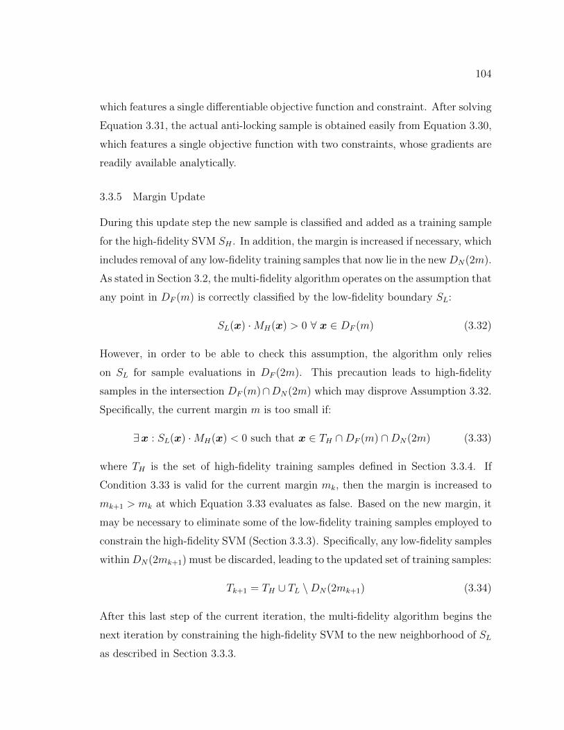
104

which features a single differentiable objective function and constraint. After solving

Equation 3.31, the actual anti-locking sample is obtained easily from Equation 3.30,

which features a single objective function with two constraints, whose gradients are

readily available analytically.

3.3.5 Margin Update

During this update step the new sample is classified and added as a training sample

for the high-fidelity SVM SH . In addition, the margin is increased if necessary, which

includes removal of any low-fidelity training samples that now lie in the newDN(2m).

As stated in Section 3.2, the multi-fidelity algorithm operates on the assumption that

any point in DF (m) is correctly classified by the low-fidelity boundary SL:

SL(x) ·MH(x) > 0 ∀ x ∈ DF (m) (3.32)

However, in order to be able to check this assumption, the algorithm only relies

on SL for sample evaluations in DF (2m). This precaution leads to high-fidelity

samples in the intersection DF (m)∩DN(2m) which may disprove Assumption 3.32.

Specifically, the current margin m is too small if:

∃x : SL(x) ·MH(x) < 0 such that x ∈ TH ∩DF (m) ∩DN(2m) (3.33)

where TH is the set of high-fidelity training samples defined in Section 3.3.4. If

Condition 3.33 is valid for the current margin mk, then the margin is increased to

mk+1 > mk at which Equation 3.33 evaluates as false. Based on the new margin, it

may be necessary to eliminate some of the low-fidelity training samples employed to

constrain the high-fidelity SVM (Section 3.3.3). Specifically, any low-fidelity samples

withinDN(2mk+1) must be discarded, leading to the updated set of training samples:

Tk+1 = TH ∪ TL \DN(2mk+1) (3.34)

After this last step of the current iteration, the multi-fidelity algorithm begins the

next iteration by constraining the high-fidelity SVM to the new neighborhood of SL

as described in Section 3.3.3.

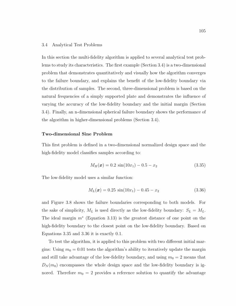
105

3.4 Analytical Test Problems

In this section the multi-fidelity algorithm is applied to several analytical test prob-

lems to study its characteristics. The first example (Section 3.4) is a two-dimensional

problem that demonstrates quantitatively and visually how the algorithm converges

to the failure boundary, and explains the benefit of the low-fidelity boundary via

the distribution of samples. The second, three-dimensional problem is based on the

natural frequencies of a simply supported plate and demonstrates the influence of

varying the accuracy of the low-fidelity boundary and the initial margin (Section

3.4). Finally, an n-dimensional spherical failure boundary shows the performance of

the algorithm in higher-dimensional problems (Section 3.4).

Two-dimensional Sine Problem

This first problem is defined in a two-dimensional normalized design space and the

high-fidelity model classifies samples according to:

MH(x) = 0.2 sin(10x1)− 0.5− x2 (3.35)

The low-fidelity model uses a similar function:

ML(x) = 0.25 sin(10x1)− 0.45− x2 (3.36)

and Figure 3.8 shows the failure boundaries corresponding to both models. For

the sake of simplicity, ML is used directly as the low-fidelity boundary: SL = ML.

The ideal margin m∗ (Equation 3.13) is the greatest distance of one point on the

high-fidelity boundary to the closest point on the low-fidelity boundary. Based on

Equations 3.35 and 3.36 it is exactly 0.1.

To test the algorithm, it is applied to this problem with two different initial mar-

gins: Using m0 = 0.01 tests the algorithm’s ability to iteratively update the margin

and still take advantage of the low-fidelity boundary, and using m0 = 2 means that

DN(m0) encompasses the whole design space and the low-fidelity boundary is ig-

nored. Therefore m0 = 2 provides a reference solution to quantify the advantage

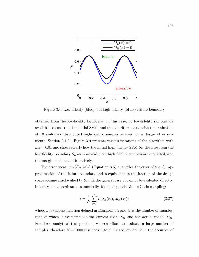
106

feasible

infeasible

x1

x2

0 0.2 0.4 0.6 0.8 10

0.2

0.4

0.6

0.8

1

ML(x) = 0MH(x) = 0

Figure 3.8: Low-fidelity (blue) and high-fidelity (black) failure boundary

obtained from the low-fidelity boundary. In this case, no low-fidelity samples are

available to construct the initial SVM, and the algorithm starts with the evaluation

of 10 uniformly distributed high-fidelity samples selected by a design of experi-

ments (Section 2.1.2). Figure 3.9 presents various iterations of the algorithm with

m0 = 0.01 and shows clearly how the initial high-fidelity SVM SH deviates from the

low-fidelity boundary SL as more and more high-fidelity samples are evaluated, and

the margin is increased iteratively.

The error measure ε(SH ,MH) (Equation 3.6) quantifies the error of the SH ap-

proximation of the failure boundary and is equivalent to the fraction of the design

space volume misclassified by SH . In the general case, it cannot be evaluated directly,

but may be approximated numerically, for example via Monte-Carlo sampling:

ε =1

N

N∑i=1

L(SH(xi),MH(xi)) (3.37)

where L is the loss function defined in Equation 3.5 and N is the number of samples,

each of which is evaluated via the current SVM SH and the actual model MH .

For these analytical test problems we can afford to evaluate a large number of

samples, therefore N = 100000 is chosen to eliminate any doubt in the accuracy of

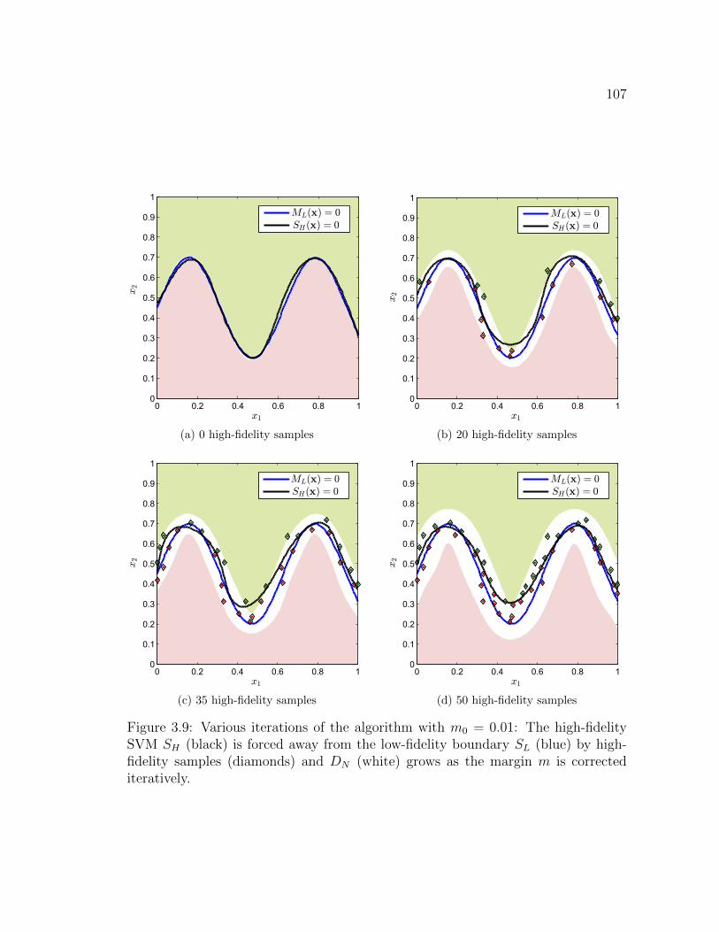
107

0 0.2 0.4 0.6 0.8 10

0.1

0.2

0.3

0.4

0.5

0.6

0.7

0.8

0.9

1

x1

x2

ML(x) = 0

SH(x) = 0

(a) 0 high-fidelity samples

0 0.2 0.4 0.6 0.8 10

0.1

0.2

0.3

0.4

0.5

0.6

0.7

0.8

0.9

1

x1

x2

ML(x) = 0

SH(x) = 0

(b) 20 high-fidelity samples

0 0.2 0.4 0.6 0.8 10

0.1

0.2

0.3

0.4

0.5

0.6

0.7

0.8

0.9

1

x1

x2

ML(x) = 0

SH(x) = 0

(c) 35 high-fidelity samples

0 0.2 0.4 0.6 0.8 10

0.1

0.2

0.3

0.4

0.5

0.6

0.7

0.8

0.9

1

x1

x2

ML(x) = 0

SH(x) = 0

(d) 50 high-fidelity samples

Figure 3.9: Various iterations of the algorithm with m0 = 0.01: The high-fidelitySVM SH (black) is forced away from the low-fidelity boundary SL (blue) by high-fidelity samples (diamonds) and DN (white) grows as the margin m is correctediteratively.

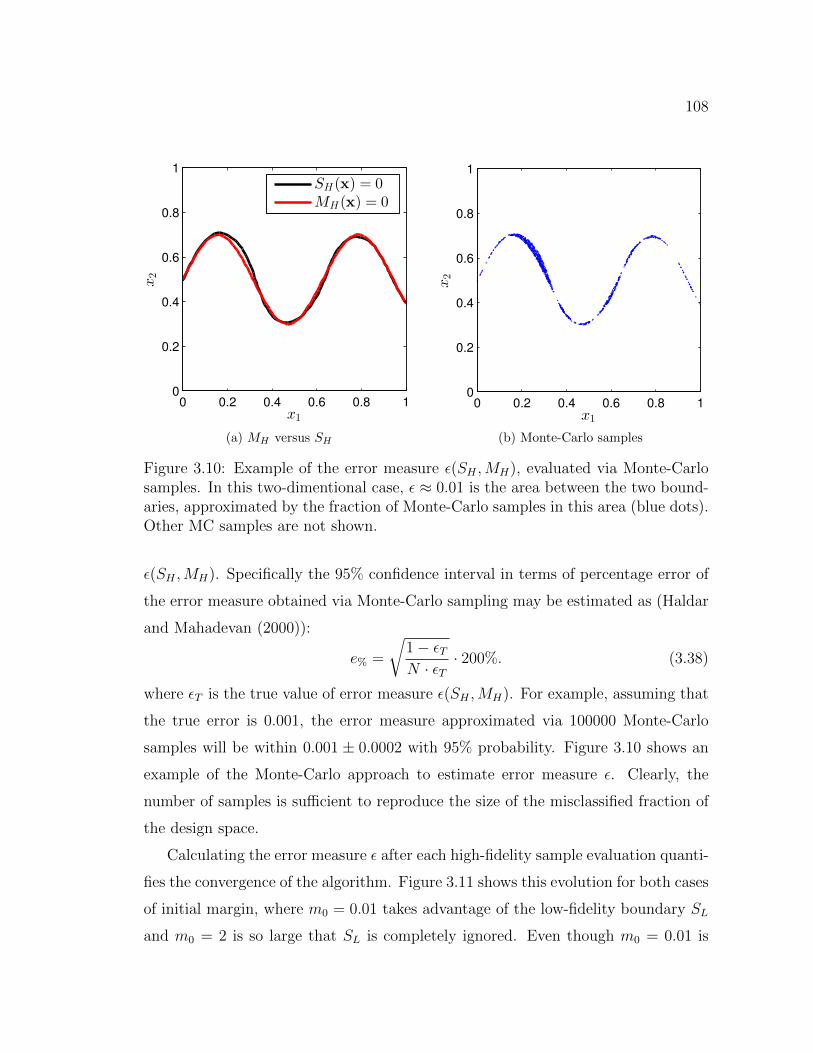
108

x1

x2

0 0.2 0.4 0.6 0.8 10

0.2

0.4

0.6

0.8

1

SH(x) = 0MH(x) = 0

(a) MH versus SH

x1

x2

0 0.2 0.4 0.6 0.8 10

0.2

0.4

0.6

0.8

1

(b) Monte-Carlo samples

Figure 3.10: Example of the error measure ε(SH ,MH), evaluated via Monte-Carlosamples. In this two-dimentional case, ε ≈ 0.01 is the area between the two bound-aries, approximated by the fraction of Monte-Carlo samples in this area (blue dots).Other MC samples are not shown.

ε(SH ,MH). Specifically the 95% confidence interval in terms of percentage error of

the error measure obtained via Monte-Carlo sampling may be estimated as (Haldar

and Mahadevan (2000)):

e% =

√1− εTN · εT

· 200%. (3.38)

where εT is the true value of error measure ε(SH ,MH). For example, assuming that

the true error is 0.001, the error measure approximated via 100000 Monte-Carlo

samples will be within 0.001 ± 0.0002 with 95% probability. Figure 3.10 shows an

example of the Monte-Carlo approach to estimate error measure ε. Clearly, the

number of samples is sufficient to reproduce the size of the misclassified fraction of

the design space.

Calculating the error measure ε after each high-fidelity sample evaluation quanti-

fies the convergence of the algorithm. Figure 3.11 shows this evolution for both cases

of initial margin, where m0 = 0.01 takes advantage of the low-fidelity boundary SL

and m0 = 2 is so large that SL is completely ignored. Even though m0 = 0.01 is

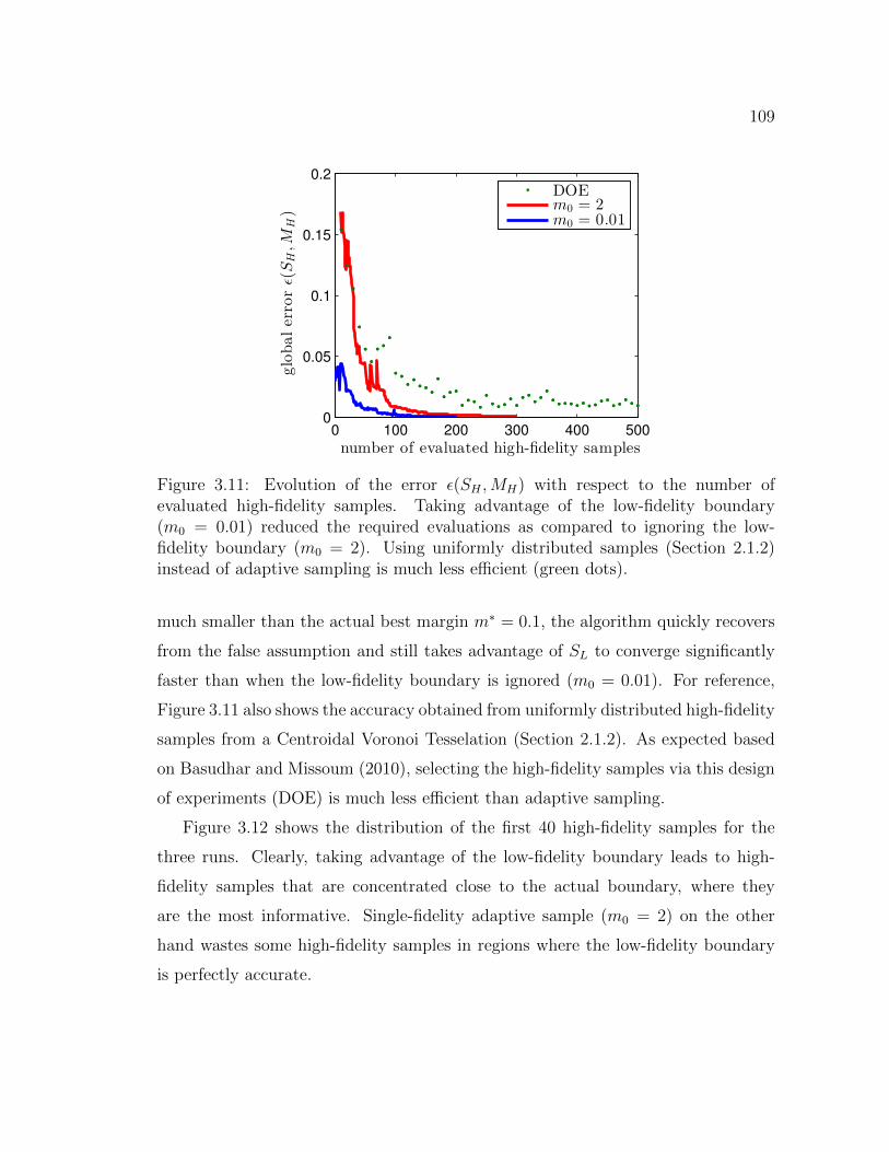
109

0 100 200 300 400 5000

0.05

0.1

0.15

0.2

number of evaluated high-fidelity samples

globalerrorǫ(S

H,M

H)

DOEm0 = 2m0 = 0.01

Figure 3.11: Evolution of the error ε(SH ,MH) with respect to the number ofevaluated high-fidelity samples. Taking advantage of the low-fidelity boundary(m0 = 0.01) reduced the required evaluations as compared to ignoring the low-fidelity boundary (m0 = 2). Using uniformly distributed samples (Section 2.1.2)instead of adaptive sampling is much less efficient (green dots).

much smaller than the actual best margin m∗ = 0.1, the algorithm quickly recovers

from the false assumption and still takes advantage of SL to converge significantly

faster than when the low-fidelity boundary is ignored (m0 = 0.01). For reference,

Figure 3.11 also shows the accuracy obtained from uniformly distributed high-fidelity

samples from a Centroidal Voronoi Tesselation (Section 2.1.2). As expected based

on Basudhar and Missoum (2010), selecting the high-fidelity samples via this design

of experiments (DOE) is much less efficient than adaptive sampling.

Figure 3.12 shows the distribution of the first 40 high-fidelity samples for the

three runs. Clearly, taking advantage of the low-fidelity boundary leads to high-

fidelity samples that are concentrated close to the actual boundary, where they

are the most informative. Single-fidelity adaptive sample (m0 = 2) on the other

hand wastes some high-fidelity samples in regions where the low-fidelity boundary

is perfectly accurate.

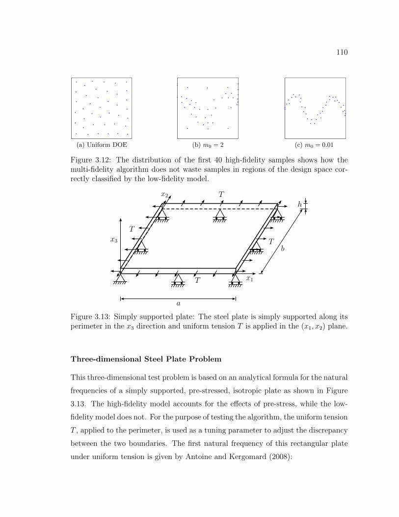
110

(a) Uniform DOE (b) m0 = 2 (c) m0 = 0.01

Figure 3.12: The distribution of the first 40 high-fidelity samples shows how themulti-fidelity algorithm does not waste samples in regions of the design space cor-rectly classified by the low-fidelity model.

T

T

T

T

x1

x2

x3

a

b

h

Figure 3.13: Simply supported plate: The steel plate is simply supported along itsperimeter in the x3 direction and uniform tension T is applied in the (x1, x2) plane.

Three-dimensional Steel Plate Problem

This three-dimensional test problem is based on an analytical formula for the natural

frequencies of a simply supported, pre-stressed, isotropic plate as shown in Figure

3.13. The high-fidelity model accounts for the effects of pre-stress, while the low-

fidelity model does not. For the purpose of testing the algorithm, the uniform tension

T , applied to the perimeter, is used as a tuning parameter to adjust the discrepancy

between the two boundaries. The first natural frequency of this rectangular plate

under uniform tension is given by Antoine and Kergomard (2008):

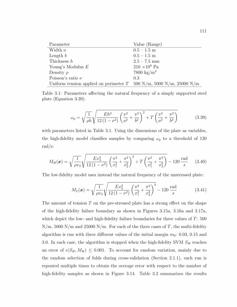
111

Parameter Value (Range)Width a 0.5 – 1.5 mLength b 0.5 – 1.5 mThickness h 2.5 – 7.5 mmYoung’s Modulus E 210 ×109 PaDensity ρ 7800 kg/m3

Poisson’s ratio ν 0.3Uniform tension applied on perimeter T 500 N/m, 5000 N/m, 25000 N/m

Table 3.1: Parameters affecting the natural frequency of a simply supported steelplate (Equation 3.39).

ωp =

√1

ρh

√Eh3

12 (1− ν2)

(π2

a2+π2

b2

)2

+ T

(π2

a2+π2

b2

)(3.39)

with parameters listed in Table 3.1. Using the dimensions of the plate as variables,

the high-fidelity model classifies samples by comparing ωp to a threshold of 120

rad/s:

MH(x) =

√1

ρx3

√Ex33

12 (1− ν2)

(π2

x21+π2

x22

)2

+ T

(π2

x21+π2

x22

)− 120

rad

s(3.40)

The low-fidelity model uses instead the natural frequency of the unstressed plate:

ML(x) =

√1

ρx3

√Ex33

12 (1− ν2)

(π2

x21+π2

x22

)2

− 120rad

s(3.41)

The amount of tension T on the pre-stressed plate has a strong effect on the shape

of the high-fidelity failure boundary as shown in Figures 3.15a, 3.16a and 3.17a,

which depict the low- and high-fidelity failure boundaries for three values of T : 500

N/m, 5000 N/m and 25000 N/m. For each of the three cases of T , the multi-fidelity

algorithm is run with three different values of the initial margin m0: 0.03, 0.15 and

3.0. In each case, the algorithm is stopped when the high-fidelity SVM SH reaches

an error of ε(SH ,MH) ≤ 0.001. To account for random variation, mainly due to

the random selection of folds during cross-validation (Section 2.1.1), each run is

repeated multiple times to obtain the average error with respect to the number of

high-fidelity samples as shown in Figure 3.14. Table 3.2 summarizes the results

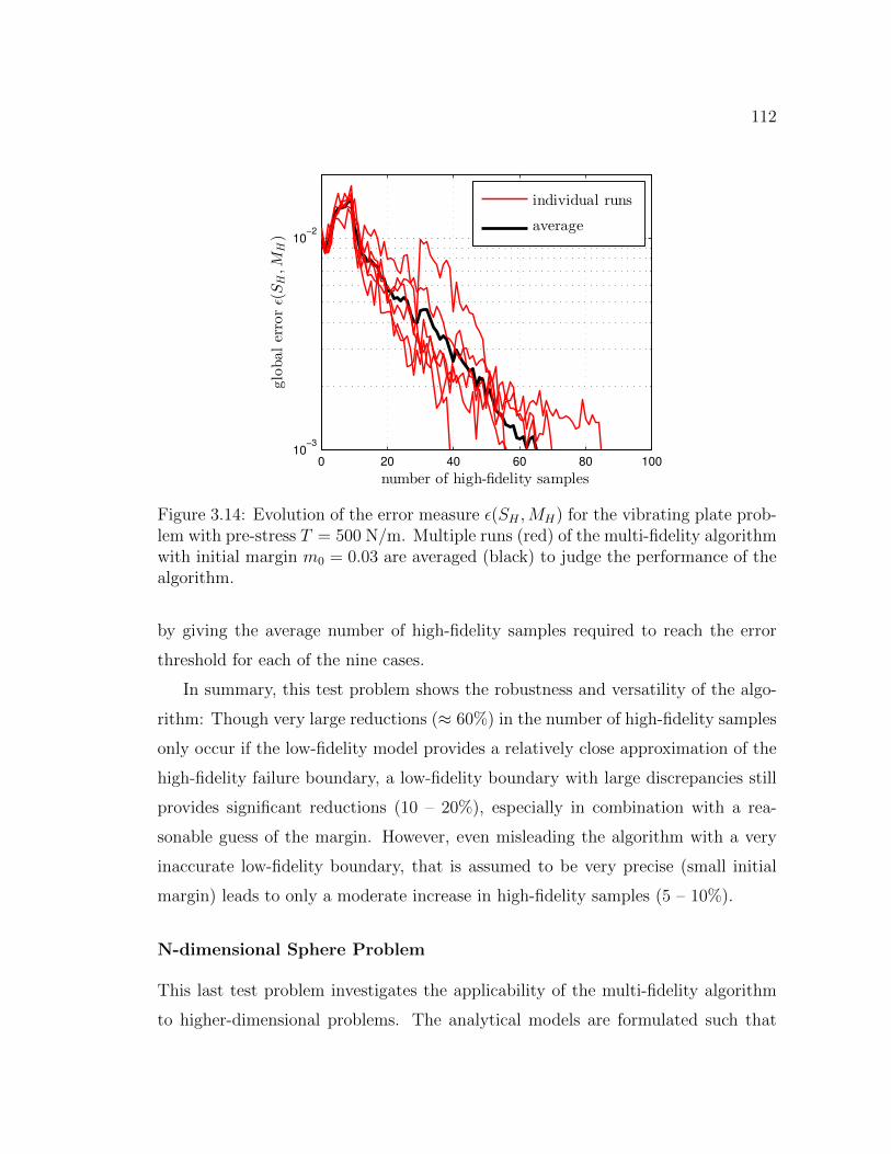
112

0 20 40 60 80 100

10−3

10−2

number of high-fidelity samples

globalerrorǫ(S

H,M

H)

individual runs

average

Figure 3.14: Evolution of the error measure ε(SH ,MH) for the vibrating plate prob-lem with pre-stress T = 500 N/m. Multiple runs (red) of the multi-fidelity algorithmwith initial margin m0 = 0.03 are averaged (black) to judge the performance of thealgorithm.

by giving the average number of high-fidelity samples required to reach the error

threshold for each of the nine cases.

In summary, this test problem shows the robustness and versatility of the algo-

rithm: Though very large reductions (≈ 60%) in the number of high-fidelity samples

only occur if the low-fidelity model provides a relatively close approximation of the

high-fidelity failure boundary, a low-fidelity boundary with large discrepancies still

provides significant reductions (10 – 20%), especially in combination with a rea-

sonable guess of the margin. However, even misleading the algorithm with a very

inaccurate low-fidelity boundary, that is assumed to be very precise (small initial

margin) leads to only a moderate increase in high-fidelity samples (5 – 10%).

N-dimensional Sphere Problem

This last test problem investigates the applicability of the multi-fidelity algorithm

to higher-dimensional problems. The analytical models are formulated such that

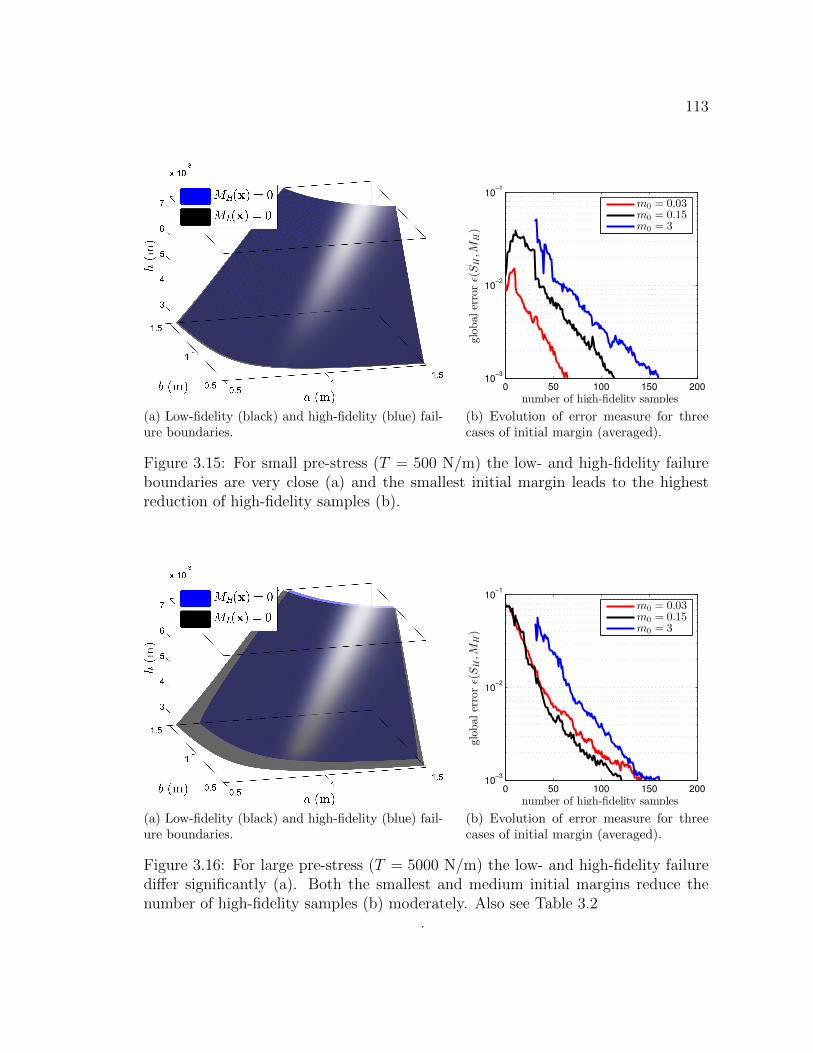
113

(a) Low-fidelity (black) and high-fidelity (blue) fail-ure boundaries.

0 50 100 150 20010

−3

10−2

10−1

number of high-fidelity samples

globalerrorǫ(S

H,M

H)

m0 = 0.03m0 = 0.15m0 = 3

(b) Evolution of error measure for threecases of initial margin (averaged).

Figure 3.15: For small pre-stress (T = 500 N/m) the low- and high-fidelity failureboundaries are very close (a) and the smallest initial margin leads to the highestreduction of high-fidelity samples (b).

(a) Low-fidelity (black) and high-fidelity (blue) fail-ure boundaries.

0 50 100 150 20010

−3

10−2

10−1

number of high-fidelity samples

global

errorǫ(S

H,M

H)

m0 = 0.03m0 = 0.15m0 = 3

(b) Evolution of error measure for threecases of initial margin (averaged).

Figure 3.16: For large pre-stress (T = 5000 N/m) the low- and high-fidelity failurediffer significantly (a). Both the smallest and medium initial margins reduce thenumber of high-fidelity samples (b) moderately. Also see Table 3.2

.

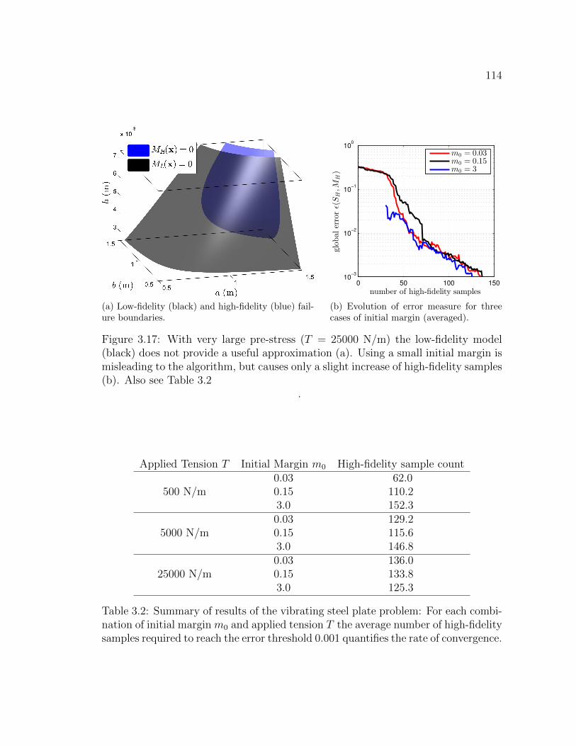
114

(a) Low-fidelity (black) and high-fidelity (blue) fail-ure boundaries.

0 50 100 15010

−3

10−2

10−1

100

number of high-fidelity samples

global

errorǫ(S

H,M

H)

m0 = 0.03m0 = 0.15m0 = 3

(b) Evolution of error measure for threecases of initial margin (averaged).

Figure 3.17: With very large pre-stress (T = 25000 N/m) the low-fidelity model(black) does not provide a useful approximation (a). Using a small initial margin ismisleading to the algorithm, but causes only a slight increase of high-fidelity samples(b). Also see Table 3.2

.

Applied Tension T Initial Margin m0 High-fidelity sample count0.03 62.0

500 N/m 0.15 110.23.0 152.30.03 129.2

5000 N/m 0.15 115.63.0 146.80.03 136.0

25000 N/m 0.15 133.83.0 125.3

Table 3.2: Summary of results of the vibrating steel plate problem: For each combi-nation of initial margin m0 and applied tension T the average number of high-fidelitysamples required to reach the error threshold 0.001 quantifies the rate of convergence.

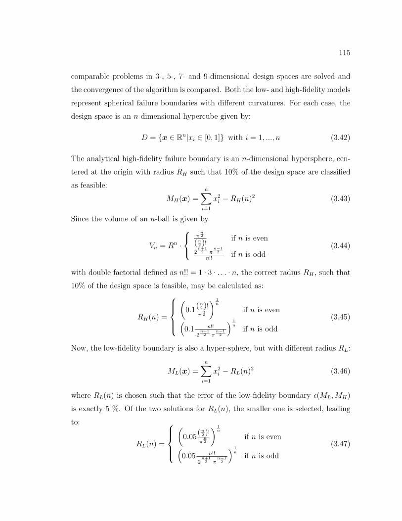
115

comparable problems in 3-, 5-, 7- and 9-dimensional design spaces are solved and

the convergence of the algorithm is compared. Both the low- and high-fidelity models

represent spherical failure boundaries with different curvatures. For each case, the

design space is an n-dimensional hypercube given by:

D = {x ∈ Rn|xi ∈ [0, 1]} with i = 1, ..., n (3.42)

The analytical high-fidelity failure boundary is an n-dimensional hypersphere, cen-

tered at the origin with radius RH such that 10% of the design space are classified

as feasible:

MH(x) =n∑i=1

x2i −RH(n)2 (3.43)

Since the volume of an n-ball is given by

Vn = Rn ·

πn2

(n2 )!if n is even

2n+12 π

n−12

n!!if n is odd

(3.44)

with double factorial defined as n!! = 1 · 3 · . . . · n, the correct radius RH , such that

10% of the design space is feasible, may be calculated as:

RH(n) =

(

0.1(n2 )!πn2

) 1n

if n is even(0.1 n!!

·2n+12 π

n−12

) 1n

if n is odd

(3.45)

Now, the low-fidelity boundary is also a hyper-sphere, but with different radius RL:

ML(x) =n∑i=1

x2i −RL(n)2 (3.46)

where RL(n) is chosen such that the error of the low-fidelity boundary ε(ML,MH)

is exactly 5 %. Of the two solutions for RL(n), the smaller one is selected, leading

to:

RL(n) =

(

0.05(n2 )!πn2

) 1n

if n is even(0.05 n!!

·2n+12 π

n−12

) 1n

if n is odd

(3.47)

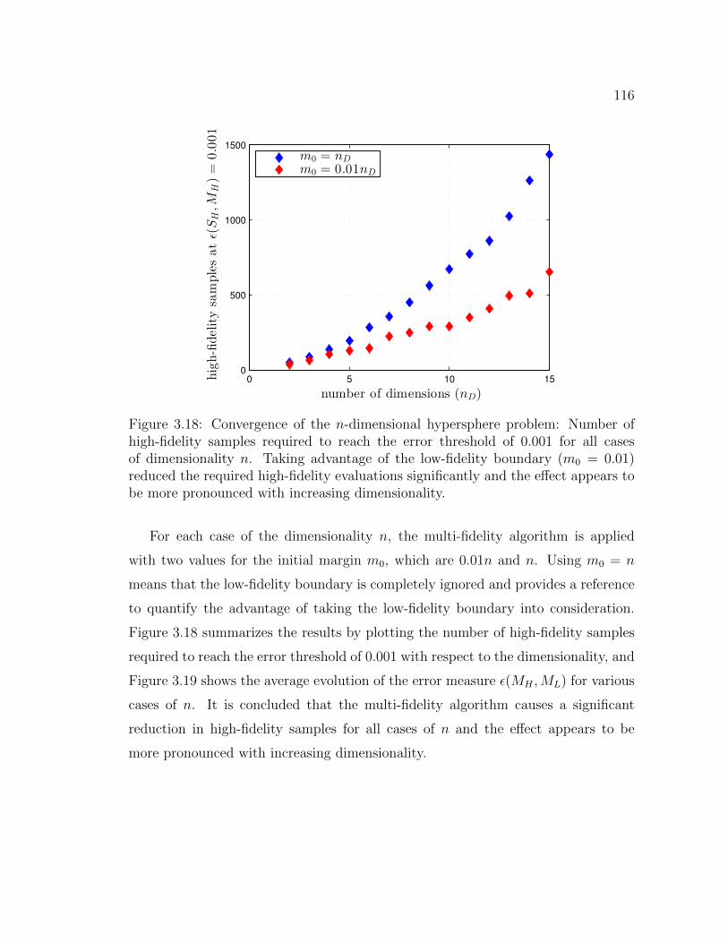
116

0 5 10 15

0

500

1000

1500

number of dimensions (nD)

high-fidelitysamplesatǫ(S

H,M

H)=

0.001

m0 = nD

m0 = 0.01nD

Figure 3.18: Convergence of the n-dimensional hypersphere problem: Number ofhigh-fidelity samples required to reach the error threshold of 0.001 for all casesof dimensionality n. Taking advantage of the low-fidelity boundary (m0 = 0.01)reduced the required high-fidelity evaluations significantly and the effect appears tobe more pronounced with increasing dimensionality.

For each case of the dimensionality n, the multi-fidelity algorithm is applied

with two values for the initial margin m0, which are 0.01n and n. Using m0 = n

means that the low-fidelity boundary is completely ignored and provides a reference

to quantify the advantage of taking the low-fidelity boundary into consideration.

Figure 3.18 summarizes the results by plotting the number of high-fidelity samples

required to reach the error threshold of 0.001 with respect to the dimensionality, and

Figure 3.19 shows the average evolution of the error measure ε(MH ,ML) for various

cases of n. It is concluded that the multi-fidelity algorithm causes a significant

reduction in high-fidelity samples for all cases of n and the effect appears to be

more pronounced with increasing dimensionality.

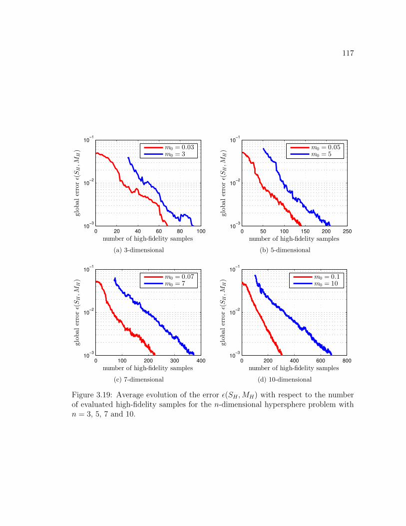
117

0 20 40 60 80 100

10−3

10−2

10−1

number of high-fidelity samples

globalerrorǫ(S

H,M

H)

m0 = 0.03m0 = 3

(a) 3-dimensional

0 50 100 150 200 250

10−3

10−2

10−1

number of high-fidelity samples

globalerrorǫ(S

H,M

H)

m0 = 0.05m0 = 5

(b) 5-dimensional

0 100 200 300 400

10−3

10−2

10−1

number of high-fidelity samples

globalerrorǫ(S

H,M

H)

m0 = 0.07m0 = 7

(c) 7-dimensional

0 200 400 600 800

10−3

10−2

10−1

number of high-fidelity samples

globalerrorǫ(S

H,M

H)

m0 = 0.1m0 = 10

(d) 10-dimensional

Figure 3.19: Average evolution of the error ε(SH ,MH) with respect to the numberof evaluated high-fidelity samples for the n-dimensional hypersphere problem withn = 3, 5, 7 and 10.

118

CHAPTER 4

AEROELASTIC STABILITY BOUNDARIES

In this section, the multi-fidelity algorithm is used to obtain the aeroelastic sta-

bility boundaries for two simulation models. The first model, proposed by Lee

et al. (1999a), simulates a rigid two degree-of-freedom airfoil, supported by non-

linear springs, in unsteady incompressible flow (Section 4.1). Here, the goal is to

obtain the stability boundary in terms of fluid velocity and initial conditions, while

taking advantage of a readily available low-fidelity stability boundary obtained from

a linear analysis assuming linear springs.

The second model (Section 4.2) simulates a finite-element model of a flexible

wing in unsteady potential flow (Section 2.3.3), using the G-method for flutter anal-

ysis (Section 2.3.3). For this problem, various simulation parameters related to

discretization affect the accuracy of the model, and two settings are defined to ob-

tain both a low-fidelity model for quick approximations and a slower high-fidelity

model for precise results.

4.1 Nonlinear Two Degree-of-Freedom Airfoil

In this section the multi-fidelity algorithm (Chapter 3) is employed to construct the

stability boundary of a rigid airfoil supported by nonlinear springs, as a function of

initial pitch conditions and reduced velocity.

Figure 4.1 schematically shows the rigid airfoil, described and analyzed in great

detail by Lee et al. (1999a), and its two degrees of freedom, which are the pitch

angle (α) and the plunge displacement (h). The airfoil is supported at the elastic

axis by nonlinear translational and rotational springs, opposing pitch and plunge,

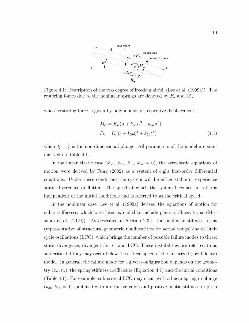
119

ah b

b

b

x b

mid-chord

elastic axis

center of massF h

M

h

Figure 4.1: Description of the two degree of freedom airfoil (Lee et al. (1999a)). Therestoring forces due to the nonlinear springs are denoted by Fh and Mα.

whose restoring force is given by polynomials of respective displacement:

Mα = Kα(α + k3αα3 + k5αα

5)

Fh = Kh(ξ + k3hξ3 + k5hξ

5) (4.1)

where ξ = hb

is the non-dimensional plunge. All parameters of the model are sum-

marized on Table 4.1.

In the linear elastic case (k3α, k5α, k3h, k5h = 0), the aeroelastic equations of

motion were derived by Fung (2002) as a system of eight first-order differential

equations. Under these conditions the system will be either stable or experience

static divergence or flutter. The speed at which the system becomes unstable is

independent of the initial conditions and is referred to as the critical speed.

In the nonlinear case, Lee et al. (1999a) derived the equations of motion for

cubic stiffnesses, which were later extended to include pentic stiffness terms (Mis-

soum et al. (2010)). As described in Section 2.3.1, the nonlinear stiffness terms

(representative of structural geometric nonlinearities for actual wings) enable limit

cycle oscillations (LCO), which brings the number of possible failure modes to three:

static divergence, divergent flutter and LCO. These instabilities are referred to as

sub-critical if they may occur below the critical speed of the linearized (low-fidelity)

model. In general, the failure mode for a given configuration depends on the geome-

try (xα, rα), the spring stiffness coefficients (Equation 4.1) and the initial conditions

(Table 4.1). For example, sub-critical LCO may occur with a linear spring in plunge

(k3h, k5h = 0) combined with a negative cubic and positive pentic stiffness in pitch

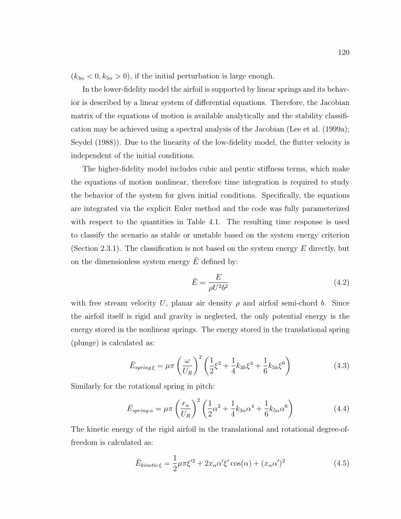
120

(k3α < 0, k5α > 0), if the initial perturbation is large enough.

In the lower-fidelity model the airfoil is supported by linear springs and its behav-

ior is described by a linear system of differential equations. Therefore, the Jacobian

matrix of the equations of motion is available analytically and the stability classifi-

cation may be achieved using a spectral analysis of the Jacobian (Lee et al. (1999a);

Seydel (1988)). Due to the linearity of the low-fidelity model, the flutter velocity is

independent of the initial conditions.

The higher-fidelity model includes cubic and pentic stiffness terms, which make

the equations of motion nonlinear, therefore time integration is required to study

the behavior of the system for given initial conditions. Specifically, the equations

are integrated via the explicit Euler method and the code was fully parameterized

with respect to the quantities in Table 4.1. The resulting time response is used

to classify the scenario as stable or unstable based on the system energy criterion

(Section 2.3.1). The classification is not based on the system energy E directly, but

on the dimensionless system energy E defined by:

E =E

ρU2b2(4.2)

with free stream velocity U , planar air density ρ and airfoil semi-chord b. Since

the airfoil itself is rigid and gravity is neglected, the only potential energy is the

energy stored in the nonlinear springs. The energy stored in the translational spring

(plunge) is calculated as:

Espring ξ = µπ

(ω

UR

)2(1

2ξ2 +

1

4k3hξ

4 +1

6k5hξ

6

)(4.3)

Similarly for the rotational spring in pitch:

Espring α = µπ

(rαUR

)2(1

2α2 +

1

4k3αα

4 +1

6k5αα

6

)(4.4)

The kinetic energy of the rigid airfoil in the translational and rotational degree-of-

freedom is calculated as:

Ekinetic ξ =1

2µπξ′2 + 2xαα

′ξ′ cos(α) + (xαα′)2 (4.5)

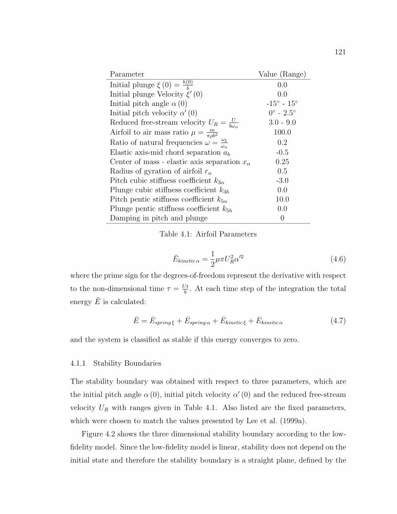
121

Parameter Value (Range)

Initial plunge ξ (0) = h(0)b

0.0Initial plunge Velocity ξ′ (0) 0.0Initial pitch angle α (0) -15◦ - 15◦

Initial pitch velocity α′ (0) 0◦ - 2.5◦

Reduced free-stream velocity UR = Ubωα

3.0 - 9.0

Airfoil to air mass ratio µ = mπρb2

100.0

Ratio of natural frequencies ω =ωξωα

0.2

Elastic axis-mid chord separation ah -0.5Center of mass - elastic axis separation xα 0.25Radius of gyration of airfoil rα 0.5Pitch cubic stiffness coefficient k3α -3.0Plunge cubic stiffness coefficient k3h 0.0Pitch pentic stiffness coefficient k5α 10.0Plunge pentic stiffness coefficient k5h 0.0Damping in pitch and plunge 0

Table 4.1: Airfoil Parameters

Ekinetic α =1

2µπU2

Rα′2 (4.6)

where the prime sign for the degrees-of-freedom represent the derivative with respect

to the non-dimensional time τ = Utb

. At each time step of the integration the total

energy E is calculated:

E = Espring ξ + Espring α + Ekinetic ξ + Ekinetic α (4.7)

and the system is classified as stable if this energy converges to zero.

4.1.1 Stability Boundaries

The stability boundary was obtained with respect to three parameters, which are

the initial pitch angle α (0), initial pitch velocity α′ (0) and the reduced free-stream

velocity UR with ranges given in Table 4.1. Also listed are the fixed parameters,

which were chosen to match the values presented by Lee et al. (1999a).

Figure 4.2 shows the three dimensional stability boundary according to the low-

fidelity model. Since the low-fidelity model is linear, stability does not depend on the

initial state and therefore the stability boundary is a straight plane, defined by the

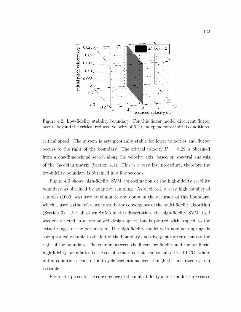
122

Figure 4.2: Low-fidelity stability boundary: For this linear model divergent flutteroccurs beyond the critical reduced velocity of 6.29, independent of initial conditions.

critical speed. The system is asymptotically stable for lower velocities and flutter

occurs to the right of the boundary. The critical velocity Uc = 6.29 is obtained

from a one-dimensional search along the velocity axis, based on spectral analysis

of the Jacobian matrix (Section 4.1). This is a very fast procedure, therefore the

low-fidelity boundary is obtained in a few seconds.

Figure 4.3 shows high-fidelity SVM approximation of the high-fidelity stability

boundary as obtained by adaptive sampling. As depicted, a very high number of

samples (1000) was used to eliminate any doubt in the accuracy of this boundary,

which is used as the reference to study the convergence of the multi-fidelity algorithm

(Section 3). Like all other SVMs in this dissertation, the high-fidelity SVM itself

was constructed in a normalized design space, but is plotted with respect to the

actual ranges of the parameters. The high-fidelity model with nonlinear springs is

asymptotically stable to the left of the boundary and divergent flutter occurs to the

right of the boundary. The volume between the linear low-fidelity and the nonlinear

high-fidelity boundaries is the set of scenarios that lead to sub-critical LCO, where

initial conditions lead to limit-cycle oscillations even though the linearized system

is stable.

Figure 4.4 presents the convergence of the multi-fidelity algorithm for three cases

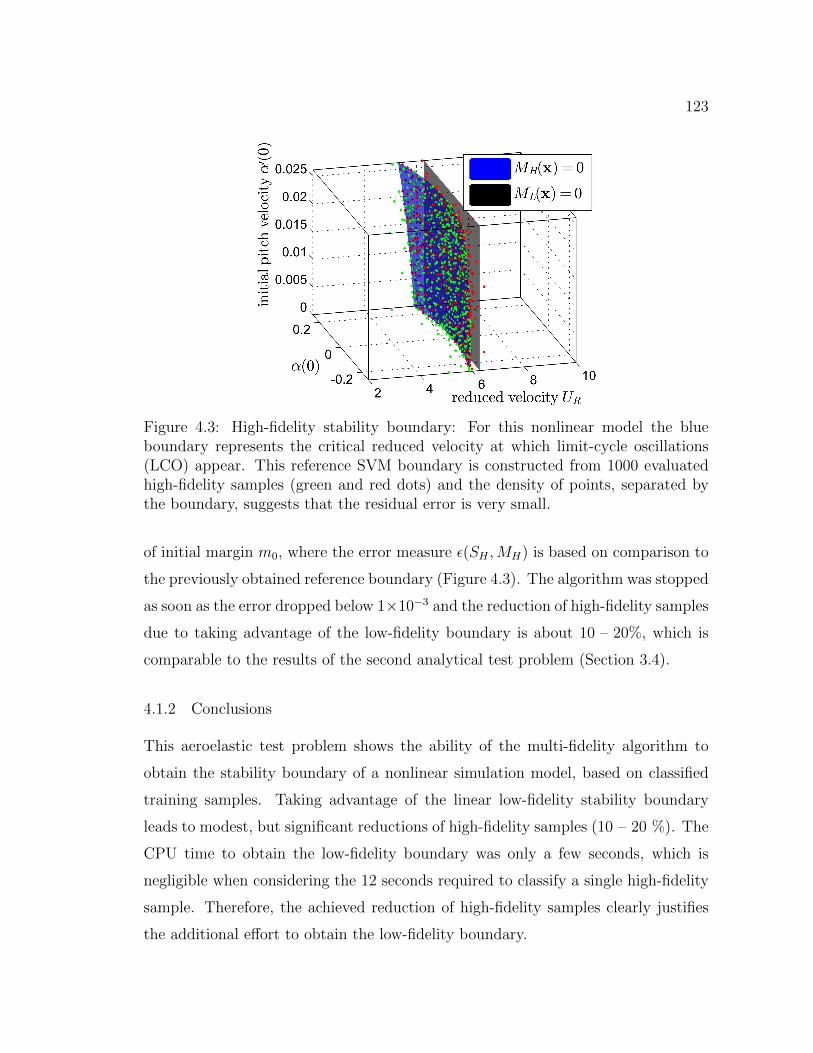
123

Figure 4.3: High-fidelity stability boundary: For this nonlinear model the blueboundary represents the critical reduced velocity at which limit-cycle oscillations(LCO) appear. This reference SVM boundary is constructed from 1000 evaluatedhigh-fidelity samples (green and red dots) and the density of points, separated bythe boundary, suggests that the residual error is very small.

of initial margin m0, where the error measure ε(SH ,MH) is based on comparison to

the previously obtained reference boundary (Figure 4.3). The algorithm was stopped

as soon as the error dropped below 1×10−3 and the reduction of high-fidelity samples

due to taking advantage of the low-fidelity boundary is about 10 – 20%, which is

comparable to the results of the second analytical test problem (Section 3.4).

4.1.2 Conclusions

This aeroelastic test problem shows the ability of the multi-fidelity algorithm to

obtain the stability boundary of a nonlinear simulation model, based on classified

training samples. Taking advantage of the linear low-fidelity stability boundary

leads to modest, but significant reductions of high-fidelity samples (10 – 20 %). The

CPU time to obtain the low-fidelity boundary was only a few seconds, which is

negligible when considering the 12 seconds required to classify a single high-fidelity

sample. Therefore, the achieved reduction of high-fidelity samples clearly justifies

the additional effort to obtain the low-fidelity boundary.

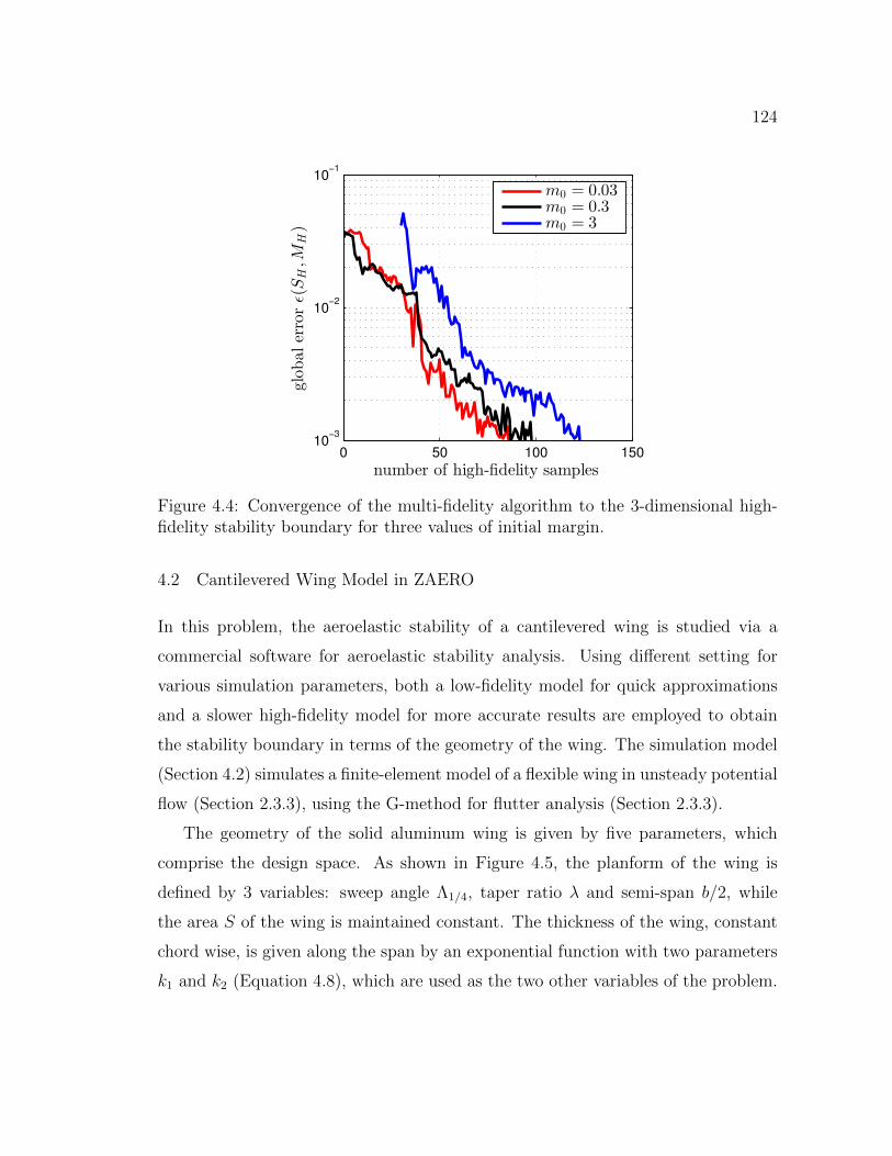
124

0 50 100 15010

−3

10−2

10−1

number of high-fidelity samples

globalerrorǫ(S

H,M

H)

m0 = 0.03m0 = 0.3m0 = 3

Figure 4.4: Convergence of the multi-fidelity algorithm to the 3-dimensional high-fidelity stability boundary for three values of initial margin.

4.2 Cantilevered Wing Model in ZAERO

In this problem, the aeroelastic stability of a cantilevered wing is studied via a

commercial software for aeroelastic stability analysis. Using different setting for

various simulation parameters, both a low-fidelity model for quick approximations

and a slower high-fidelity model for more accurate results are employed to obtain

the stability boundary in terms of the geometry of the wing. The simulation model

(Section 4.2) simulates a finite-element model of a flexible wing in unsteady potential

flow (Section 2.3.3), using the G-method for flutter analysis (Section 2.3.3).

The geometry of the solid aluminum wing is given by five parameters, which

comprise the design space. As shown in Figure 4.5, the planform of the wing is

defined by 3 variables: sweep angle Λ1/4, taper ratio λ and semi-span b/2, while

the area S of the wing is maintained constant. The thickness of the wing, constant

chord wise, is given along the span by an exponential function with two parameters

k1 and k2 (Equation 4.8), which are used as the two other variables of the problem.

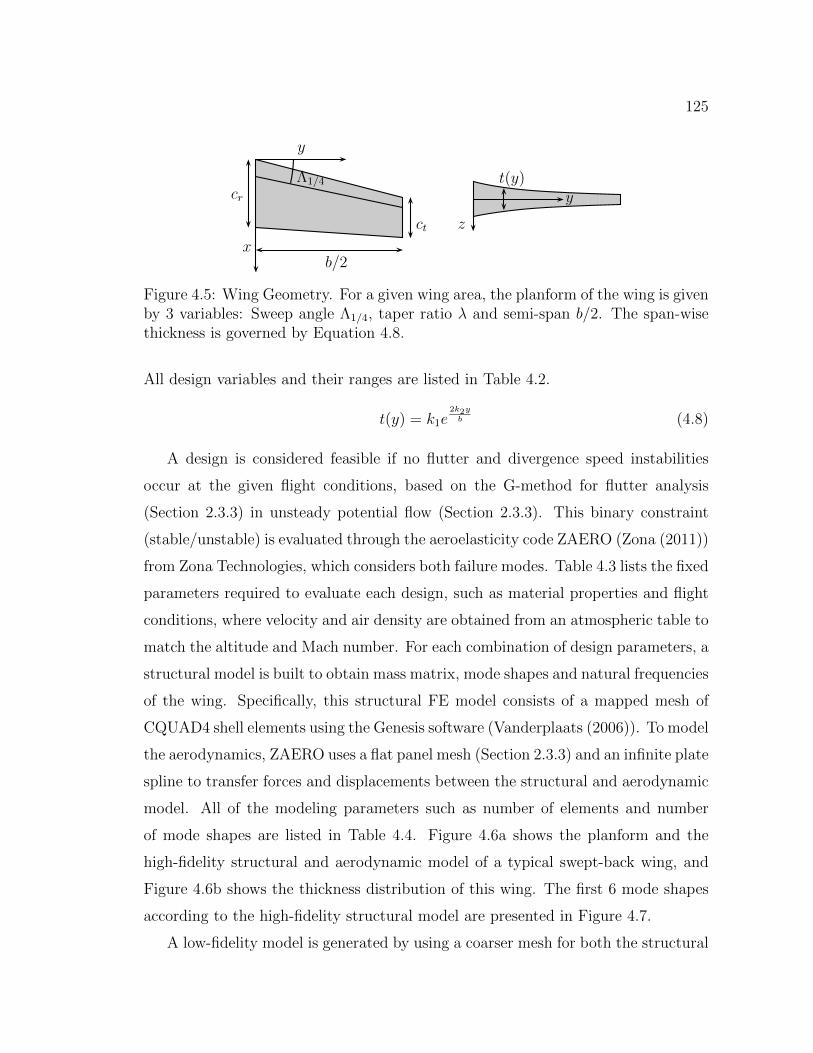
125

ct

cr

y

xb/2

Λ1/4 t(y)y

z

Figure 4.5: Wing Geometry. For a given wing area, the planform of the wing is givenby 3 variables: Sweep angle Λ1/4, taper ratio λ and semi-span b/2. The span-wisethickness is governed by Equation 4.8.

All design variables and their ranges are listed in Table 4.2.

t(y) = k1e2k2yb (4.8)

A design is considered feasible if no flutter and divergence speed instabilities

occur at the given flight conditions, based on the G-method for flutter analysis

(Section 2.3.3) in unsteady potential flow (Section 2.3.3). This binary constraint

(stable/unstable) is evaluated through the aeroelasticity code ZAERO (Zona (2011))

from Zona Technologies, which considers both failure modes. Table 4.3 lists the fixed

parameters required to evaluate each design, such as material properties and flight

conditions, where velocity and air density are obtained from an atmospheric table to

match the altitude and Mach number. For each combination of design parameters, a

structural model is built to obtain mass matrix, mode shapes and natural frequencies

of the wing. Specifically, this structural FE model consists of a mapped mesh of

CQUAD4 shell elements using the Genesis software (Vanderplaats (2006)). To model

the aerodynamics, ZAERO uses a flat panel mesh (Section 2.3.3) and an infinite plate

spline to transfer forces and displacements between the structural and aerodynamic

model. All of the modeling parameters such as number of elements and number

of mode shapes are listed in Table 4.4. Figure 4.6a shows the planform and the

high-fidelity structural and aerodynamic model of a typical swept-back wing, and

Figure 4.6b shows the thickness distribution of this wing. The first 6 mode shapes

according to the high-fidelity structural model are presented in Figure 4.7.

A low-fidelity model is generated by using a coarser mesh for both the structural

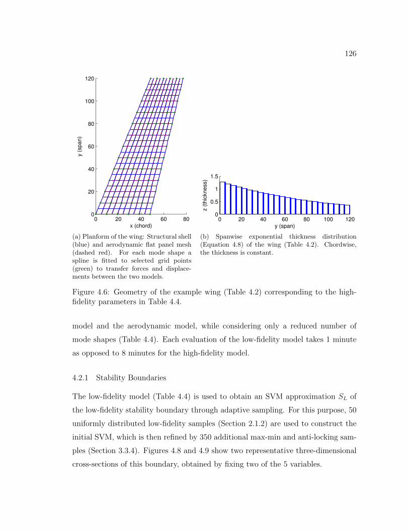
126

0 20 40 60 800

20

40

60

80

100

120

x (chord)

y (

sp

an

)

(a) Planform of the wing: Structural shell(blue) and aerodynamic flat panel mesh(dashed red). For each mode shape aspline is fitted to selected grid points(green) to transfer forces and displace-ments between the two models.

0 20 40 60 80 100 1200

0.5

1

1.5

y (span)

z (

thic

kn

ess)

(b) Spanwise exponential thickness distribution(Equation 4.8) of the wing (Table 4.2). Chordwise,the thickness is constant.

Figure 4.6: Geometry of the example wing (Table 4.2) corresponding to the high-fidelity parameters in Table 4.4.

model and the aerodynamic model, while considering only a reduced number of

mode shapes (Table 4.4). Each evaluation of the low-fidelity model takes 1 minute

as opposed to 8 minutes for the high-fidelity model.

4.2.1 Stability Boundaries

The low-fidelity model (Table 4.4) is used to obtain an SVM approximation SL of

the low-fidelity stability boundary through adaptive sampling. For this purpose, 50

uniformly distributed low-fidelity samples (Section 2.1.2) are used to construct the

initial SVM, which is then refined by 350 additional max-min and anti-locking sam-

ples (Section 3.3.4). Figures 4.8 and 4.9 show two representative three-dimensional

cross-sections of this boundary, obtained by fixing two of the 5 variables.

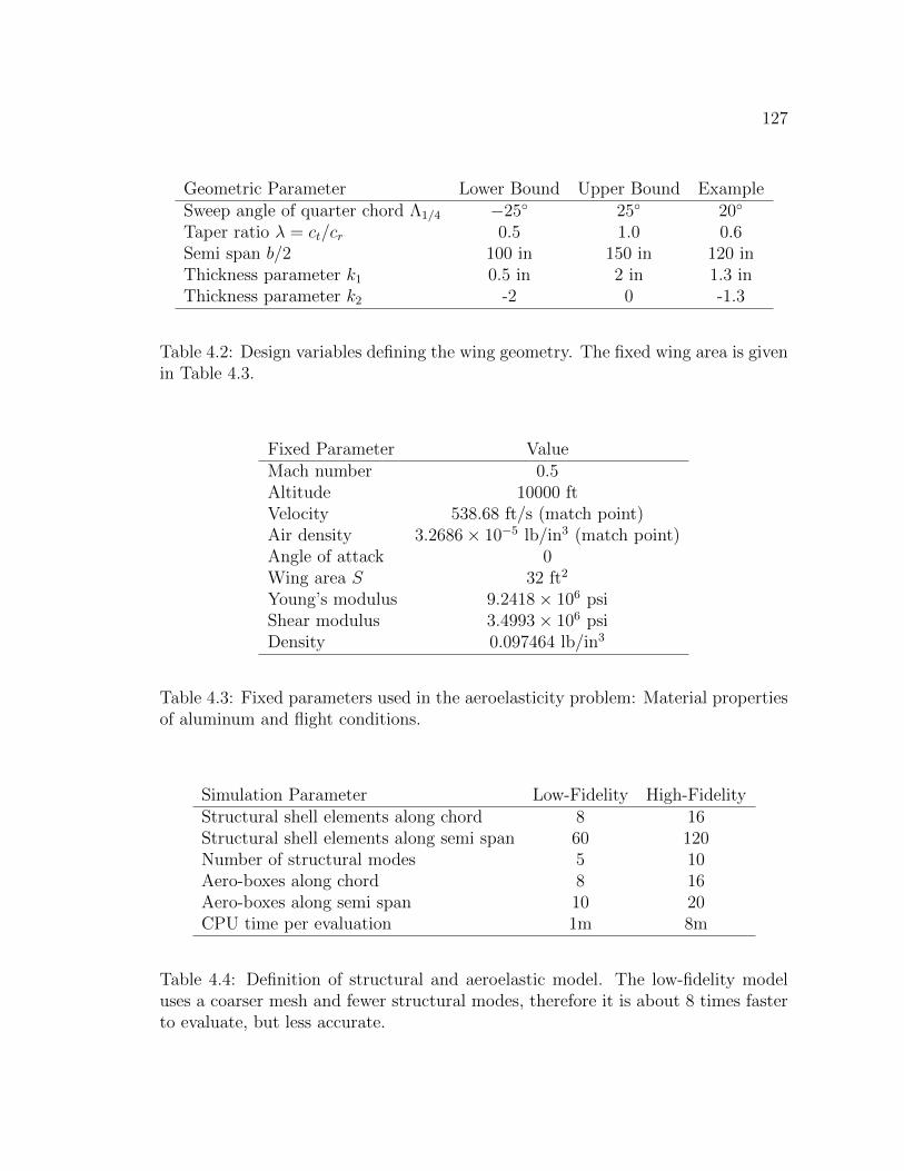
127

Geometric Parameter Lower Bound Upper Bound ExampleSweep angle of quarter chord Λ1/4 −25◦ 25◦ 20◦

Taper ratio λ = ct/cr 0.5 1.0 0.6Semi span b/2 100 in 150 in 120 inThickness parameter k1 0.5 in 2 in 1.3 inThickness parameter k2 -2 0 -1.3

Table 4.2: Design variables defining the wing geometry. The fixed wing area is givenin Table 4.3.

Fixed Parameter ValueMach number 0.5Altitude 10000 ftVelocity 538.68 ft/s (match point)Air density 3.2686× 10−5 lb/in3 (match point)Angle of attack 0Wing area S 32 ft2

Young’s modulus 9.2418× 106 psiShear modulus 3.4993× 106 psiDensity 0.097464 lb/in3

Table 4.3: Fixed parameters used in the aeroelasticity problem: Material propertiesof aluminum and flight conditions.

Simulation Parameter Low-Fidelity High-FidelityStructural shell elements along chord 8 16Structural shell elements along semi span 60 120Number of structural modes 5 10Aero-boxes along chord 8 16Aero-boxes along semi span 10 20CPU time per evaluation 1m 8m

Table 4.4: Definition of structural and aeroelastic model. The low-fidelity modeluses a coarser mesh and fewer structural modes, therefore it is about 8 times fasterto evaluate, but less accurate.

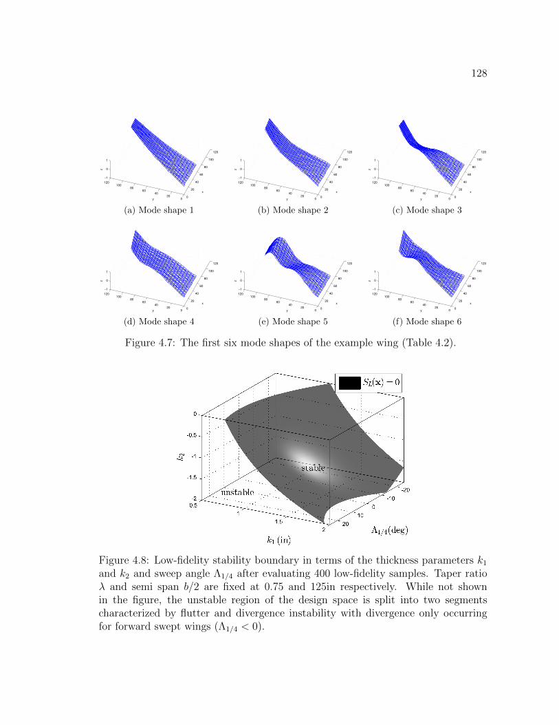
128

0

20

40

60

80

100

120

020

4060

80100

120

−1

0

1

x

y

z

(a) Mode shape 1

0

20

40

60

80

100

120

020

4060

80100

120

−1

0

1

x

y

z

(b) Mode shape 2

0

20

40

60

80

100

120

020

4060

80100

120

−1

0

1

x

y

z

(c) Mode shape 3

0

20

40

60

80

100

120

020

4060

80100

120

−1

0

1

x

y

z

(d) Mode shape 4

0

20

40

60

80

100

120

020

4060

80100

120

−1

0

1

x

y

z

(e) Mode shape 5

0

20

40

60

80

100

120

020

4060

80100

120

−1

0

1

x

y

z

(f) Mode shape 6

Figure 4.7: The first six mode shapes of the example wing (Table 4.2).

Figure 4.8: Low-fidelity stability boundary in terms of the thickness parameters k1and k2 and sweep angle Λ1/4 after evaluating 400 low-fidelity samples. Taper ratioλ and semi span b/2 are fixed at 0.75 and 125in respectively. While not shownin the figure, the unstable region of the design space is split into two segmentscharacterized by flutter and divergence instability with divergence only occurringfor forward swept wings (Λ1/4 < 0).

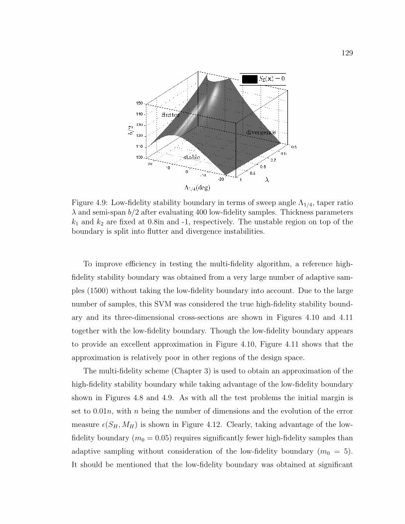
129

Figure 4.9: Low-fidelity stability boundary in terms of sweep angle Λ1/4, taper ratioλ and semi-span b/2 after evaluating 400 low-fidelity samples. Thickness parametersk1 and k2 are fixed at 0.8in and -1, respectively. The unstable region on top of theboundary is split into flutter and divergence instabilities.

To improve efficiency in testing the multi-fidelity algorithm, a reference high-

fidelity stability boundary was obtained from a very large number of adaptive sam-

ples (1500) without taking the low-fidelity boundary into account. Due to the large

number of samples, this SVM was considered the true high-fidelity stability bound-

ary and its three-dimensional cross-sections are shown in Figures 4.10 and 4.11

together with the low-fidelity boundary. Though the low-fidelity boundary appears

to provide an excellent approximation in Figure 4.10, Figure 4.11 shows that the

approximation is relatively poor in other regions of the design space.

The multi-fidelity scheme (Chapter 3) is used to obtain an approximation of the

high-fidelity stability boundary while taking advantage of the low-fidelity boundary

shown in Figures 4.8 and 4.9. As with all the test problems the initial margin is

set to 0.01n, with n being the number of dimensions and the evolution of the error

measure ε(SH ,MH) is shown in Figure 4.12. Clearly, taking advantage of the low-

fidelity boundary (m0 = 0.05) requires significantly fewer high-fidelity samples than

adaptive sampling without consideration of the low-fidelity boundary (m0 = 5).

It should be mentioned that the low-fidelity boundary was obtained at significant

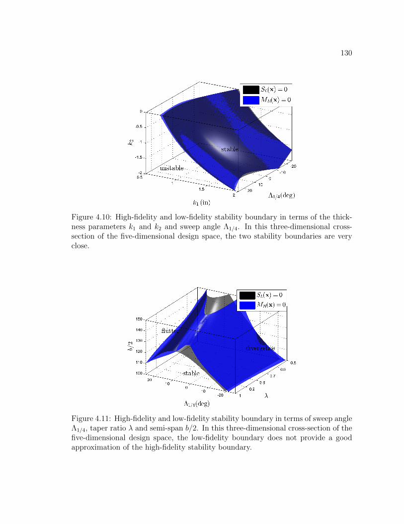
130

Figure 4.10: High-fidelity and low-fidelity stability boundary in terms of the thick-ness parameters k1 and k2 and sweep angle Λ1/4. In this three-dimensional cross-section of the five-dimensional design space, the two stability boundaries are veryclose.

Figure 4.11: High-fidelity and low-fidelity stability boundary in terms of sweep angleΛ1/4, taper ratio λ and semi-span b/2. In this three-dimensional cross-section of thefive-dimensional design space, the low-fidelity boundary does not provide a goodapproximation of the high-fidelity stability boundary.

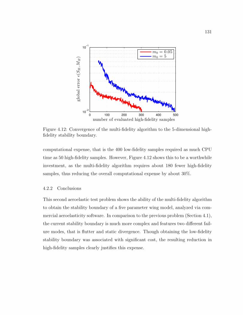
131

0 100 200 300 400 500

10−2

10−1

number of evaluated high-fidelity samples

globalerrorǫ(S

H,M

H)

m0 = 0.05m0 = 5

Figure 4.12: Convergence of the multi-fidelity algorithm to the 5-dimensional high-fidelity stability boundary.

computational expense, that is the 400 low-fidelity samples required as much CPU

time as 50 high-fidelity samples. However, Figure 4.12 shows this to be a worthwhile

investment, as the multi-fidelity algorithm requires about 180 fewer high-fidelity

samples, thus reducing the overall computational expense by about 30%.

4.2.2 Conclusions

This second aeroelastic test problem shows the ability of the multi-fidelity algorithm

to obtain the stability boundary of a five parameter wing model, analyzed via com-

mercial aeroelasticity software. In comparison to the previous problem (Section 4.1),

the current stability boundary is much more complex and features two different fail-

ure modes, that is flutter and static divergence. Though obtaining the low-fidelity

stability boundary was associated with significant cost, the resulting reduction in

high-fidelity samples clearly justifies this expense.

132

CHAPTER 5

MULTI-FIDELITY OPTIMIZATION

The multi-fidelity algorithm described in Chapter 3 seeks to construct an SVM

constraint boundary that is accurate over the whole design space. However, for the

purpose of numerical design optimization, it may be advantageous to limit high-

fidelity samples to regions of the design space that are likely to contain the optimal

design. Assuming a low evaluation cost of the objective function to minimize, this

can be achieved by only a small modification of the multi-fidelity algorithm as

presented in this section.

The main premise of this variant is the following: As soon as the algorithm

has discovered a sample that is classified as feasible by the high-fidelity constraint

model, it is wasteful to evaluate any other sample via the high-fidelity constraint,

unless its objective function value is lower. To eliminate such waste, any high-fidelity

sample xi selected by the multi-fidelity algorithm is first evaluated via the objective

function. If its value is higher than the current best feasible sample x∗, then the

new sample xi is not evaluated via the high-fidelity constraint function, but instead

added to the set of blocked samples Xb. This set of samples is ignored for the purpose

of training the SVM, but treated as existing samples during the adaptive sampling

(Section 3.3.4). Blocking samples in this way prevents the algorithm from selecting

the same point again and forces the adaptive sampling routine to find max-min or

anti-locking samples with lower objective function value than the current optimum

x∗k.

This straight-forward modification requires only a small change to the imple-

mentation (Figure 5.1) and reduces the computational burden significantly if one

only seeks to obtain the constrained optimum with respect to an inexpensive objec-

tive function. Unfortunately, this modification is not well suited for the case where

evaluating the objective function is associated with significant cost, unless the ob-

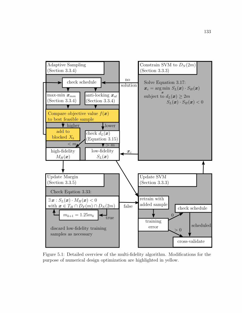
133

Update Margin(Section 3.3.5)

Update SVM(Section 3.3.3)

Adaptive Sampling(Section 3.3.4)

Check Eqation 3.33:

cross-validate

check schedule

Solve Equation 3.17:xc = arg min

xSL(x) · SH(x)

subject to dL(x) ≥ 2mSL(x) · SH(x) < 0

check schedule

> m< m

0

> 0scheduled

Constrain SVM to DN(2m)(Section 3.3.3)

xc

nosolution

max-min xmm(Section 3.3.4)

anti-locking xal(Section 3.3.4)

check dL(x)(Equation 3.15)

high-fidelityMH(x)

low-fidelitySL(x)

mk+1 = 1.25mk

∃x : SL(x) ·MH(x) < 0with x ∈ TH ∩DF (m) ∩DN(2m) false

true

retrain withadded sample

trainingerrordiscard low-fidelity training

samples as necessary

Compare objective value f(x)to best feasible sample

add toblocked Xb

higher lower

Figure 5.1: Detailed overview of the multi-fidelity algorithm. Modifications for thepurpose of numerical design optimization are highlighted in yellow.

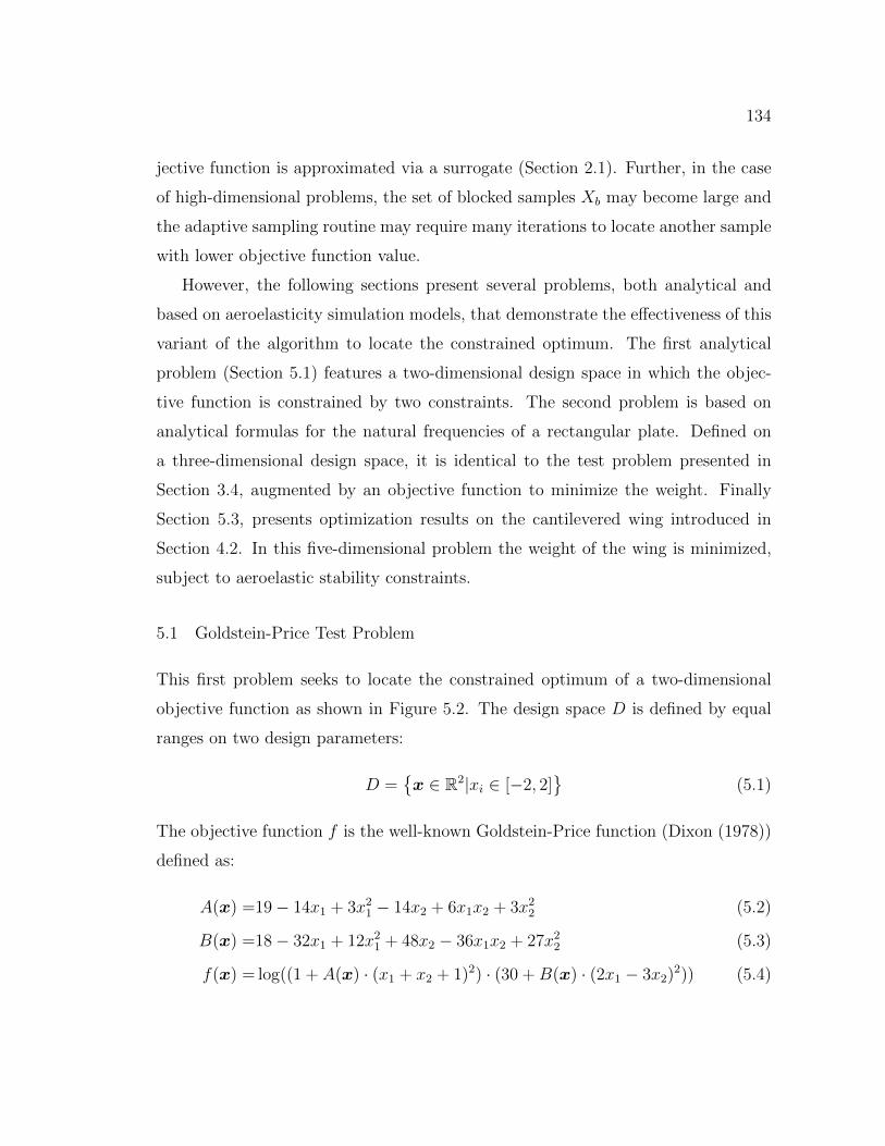
134

jective function is approximated via a surrogate (Section 2.1). Further, in the case

of high-dimensional problems, the set of blocked samples Xb may become large and

the adaptive sampling routine may require many iterations to locate another sample

with lower objective function value.

However, the following sections present several problems, both analytical and

based on aeroelasticity simulation models, that demonstrate the effectiveness of this

variant of the algorithm to locate the constrained optimum. The first analytical

problem (Section 5.1) features a two-dimensional design space in which the objec-

tive function is constrained by two constraints. The second problem is based on

analytical formulas for the natural frequencies of a rectangular plate. Defined on

a three-dimensional design space, it is identical to the test problem presented in

Section 3.4, augmented by an objective function to minimize the weight. Finally

Section 5.3, presents optimization results on the cantilevered wing introduced in

Section 4.2. In this five-dimensional problem the weight of the wing is minimized,

subject to aeroelastic stability constraints.

5.1 Goldstein-Price Test Problem

This first problem seeks to locate the constrained optimum of a two-dimensional

objective function as shown in Figure 5.2. The design space D is defined by equal

ranges on two design parameters:

D ={x ∈ R2|xi ∈ [−2, 2]

}(5.1)

The objective function f is the well-known Goldstein-Price function (Dixon (1978))

defined as:

A(x) =19− 14x1 + 3x21 − 14x2 + 6x1x2 + 3x22 (5.2)

B(x) =18− 32x1 + 12x21 + 48x2 − 36x1x2 + 27x22 (5.3)

f(x) = log((1 + A(x) · (x1 + x2 + 1)2) · (30 +B(x) · (2x1 − 3x2)2)) (5.4)

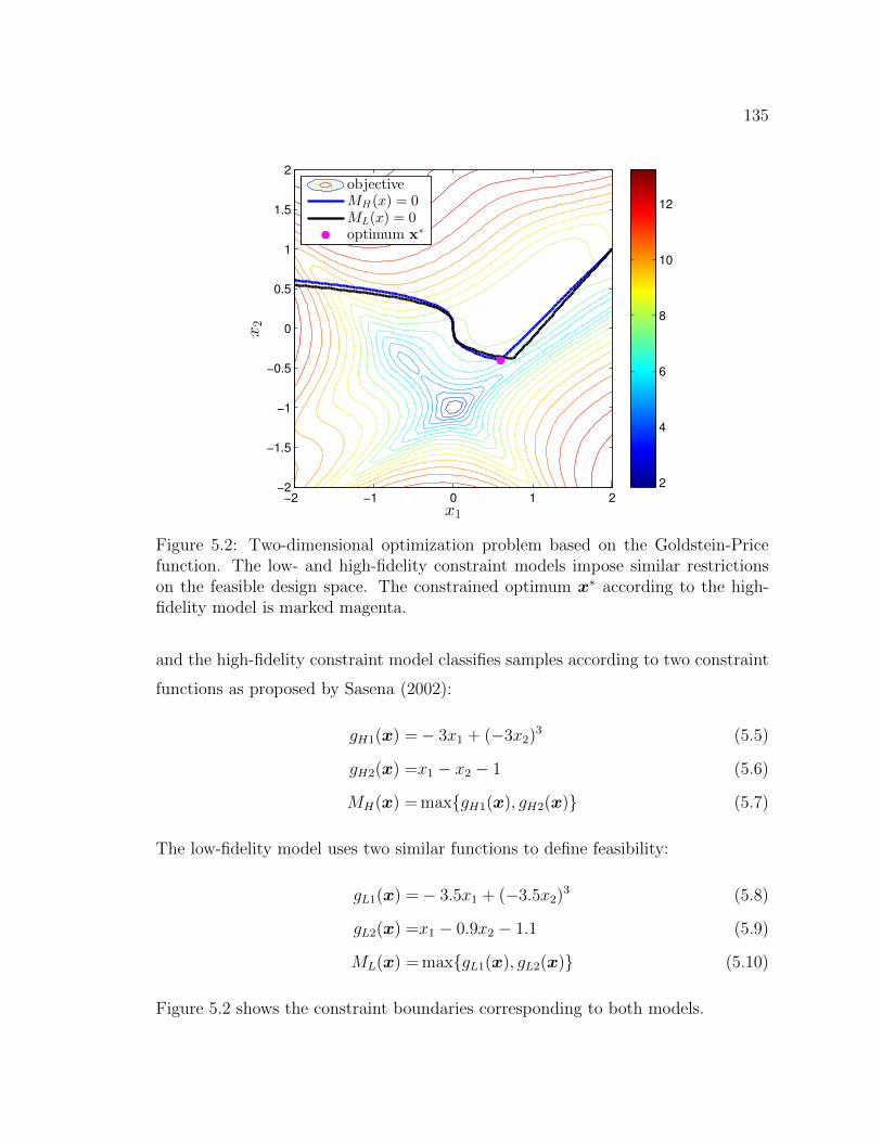
135

x1

x2

−2 −1 0 1 2−2

−1.5

−1

−0.5

0

0.5

1

1.5

2

objectiveMH(x) = 0ML(x) = 0optimum x

∗

2

4

6

8

10

12

Figure 5.2: Two-dimensional optimization problem based on the Goldstein-Pricefunction. The low- and high-fidelity constraint models impose similar restrictionson the feasible design space. The constrained optimum x∗ according to the high-fidelity model is marked magenta.

and the high-fidelity constraint model classifies samples according to two constraint

functions as proposed by Sasena (2002):

gH1(x) =− 3x1 + (−3x2)3 (5.5)

gH2(x) =x1 − x2 − 1 (5.6)

MH(x) = max{gH1(x), gH2(x)} (5.7)

The low-fidelity model uses two similar functions to define feasibility:

gL1(x) =− 3.5x1 + (−3.5x2)3 (5.8)

gL2(x) =x1 − 0.9x2 − 1.1 (5.9)

ML(x) = max{gL1(x), gL2(x)} (5.10)

Figure 5.2 shows the constraint boundaries corresponding to both models.

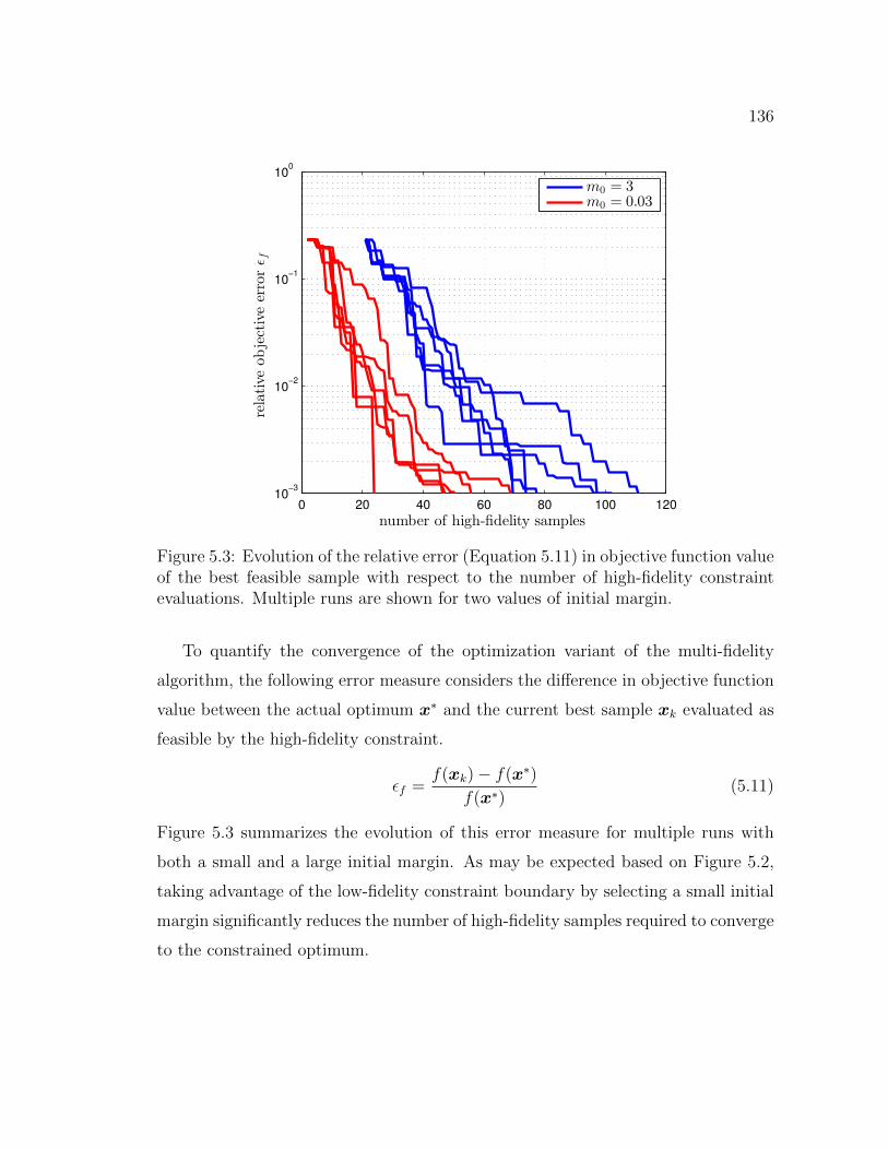
136

0 20 40 60 80 100 12010

−3

10−2

10−1

100

number of high-fidelity samples

relativeobjectiveerrorǫf

m0 = 3m0 = 0.03

Figure 5.3: Evolution of the relative error (Equation 5.11) in objective function valueof the best feasible sample with respect to the number of high-fidelity constraintevaluations. Multiple runs are shown for two values of initial margin.

To quantify the convergence of the optimization variant of the multi-fidelity

algorithm, the following error measure considers the difference in objective function

value between the actual optimum x∗ and the current best sample xk evaluated as

feasible by the high-fidelity constraint.

εf =f(xk)− f(x∗)

f(x∗)(5.11)

Figure 5.3 summarizes the evolution of this error measure for multiple runs with

both a small and a large initial margin. As may be expected based on Figure 5.2,

taking advantage of the low-fidelity constraint boundary by selecting a small initial

margin significantly reduces the number of high-fidelity samples required to converge

to the constrained optimum.

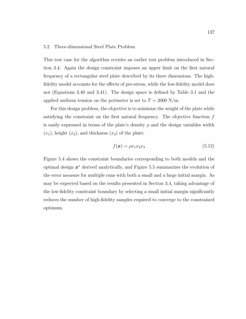
137

5.2 Three-dimensional Steel Plate Problem

This test case for the algorithm revisits an earlier test problem introduced in Sec-

tion 3.4. Again the design constraint imposes an upper limit on the first natural

frequency of a rectangular steel plate described by its three dimensions. The high-

fidelity model accounts for the effects of pre-stress, while the low-fidelity model does

not (Equations 3.40 and 3.41). The design space is defined by Table 3.1 and the

applied uniform tension on the perimeter is set to T = 2000 N/m.

For this design problem, the objective is to minimize the weight of the plate while

satisfying the constraint on the first natural frequency. The objective function f

is easily expressed in terms of the plate’s density ρ and the design variables width

(x1), height (x2), and thickness (x3) of the plate:

f(x) = ρx1x2x3 (5.12)

Figure 5.4 shows the constraint boundaries corresponding to both models and the

optimal design x∗ derived analytically, and Figure 5.5 summarizes the evolution of

the error measure for multiple runs with both a small and a large initial margin. As

may be expected based on the results presented in Section 3.4, taking advantage of

the low-fidelity constraint boundary by selecting a small initial margin significantly

reduces the number of high-fidelity samples required to converge to the constrained

optimum.

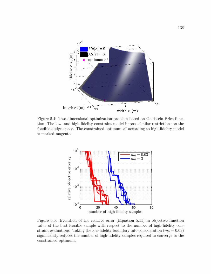
138

Figure 5.4: Two-dimensional optimization problem based on Goldstein-Price func-tion. The low- and high-fidelity constraint model impose similar restrictions on thefeasible design space. The constrained optimum x∗ according to high-fidelity modelis marked magenta.

0 20 40 60 8010

−3

10−2

10−1

100

number of high-fidelity samples

relativeobjectiveerrorǫf

m0 = 0.03m0 = 3

Figure 5.5: Evolution of the relative error (Equation 5.11) in objective functionvalue of the best feasible sample with respect to the number of high-fidelity con-straint evaluations. Taking the low-fidelity boundary into consideration (m0 = 0.03)significantly reduces the number of high-fidelity samples required to converge to theconstrained optimum.

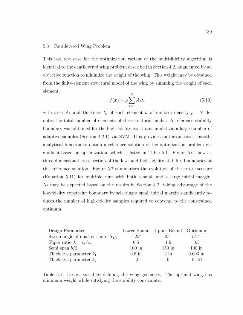
139

5.3 Cantilevered Wing Problem

This last test case for the optimization variant of the multi-fidelity algorithm is

identical to the cantilevered wing problem described in Section 4.2, augmented by an

objective function to minimize the weight of the wing. This weight may be obtained

from the finite-element structural model of the wing by summing the weight of each

element:

f(x) = ρN∑k=1

Aktk (5.13)

with area Ak and thickness tk of shell element k of uniform density ρ. N de-

notes the total number of elements of the structural model. A reference stability

boundary was obtained for the high-fidelity constraint model via a large number of

adaptive samples (Section 4.2.1) via SVM. This provides an inexpensive, smooth,

analytical function to obtain a reference solution of the optimization problem via

gradient-based on optimization, which is listed in Table 5.1. Figure 5.6 shows a

three-dimensional cross-section of the low- and high-fidelity stability boundaries at

this reference solution. Figure 5.7 summarizes the evolution of the error measure

(Equation 5.11) for multiple runs with both a small and a large initial margin.

As may be expected based on the results in Section 4.2, taking advantage of the

low-fidelity constraint boundary by selecting a small initial margin significantly re-

duces the number of high-fidelity samples required to converge to the constrained

optimum.

Design Parameter Lower Bound Upper Bound OptimumSweep angle of quarter chord Λ1/4 −25◦ 25◦ 7.74◦

Taper ratio λ = ct/cr 0.5 1.0 0.5Semi span b/2 100 in 150 in 100 inThickness parameter k1 0.5 in 2 in 0.603 inThickness parameter k2 -2 0 -0.454

Table 5.1: Design variables defining the wing geometry. The optimal wing hasminimum weight while satisfying the stability constraints.

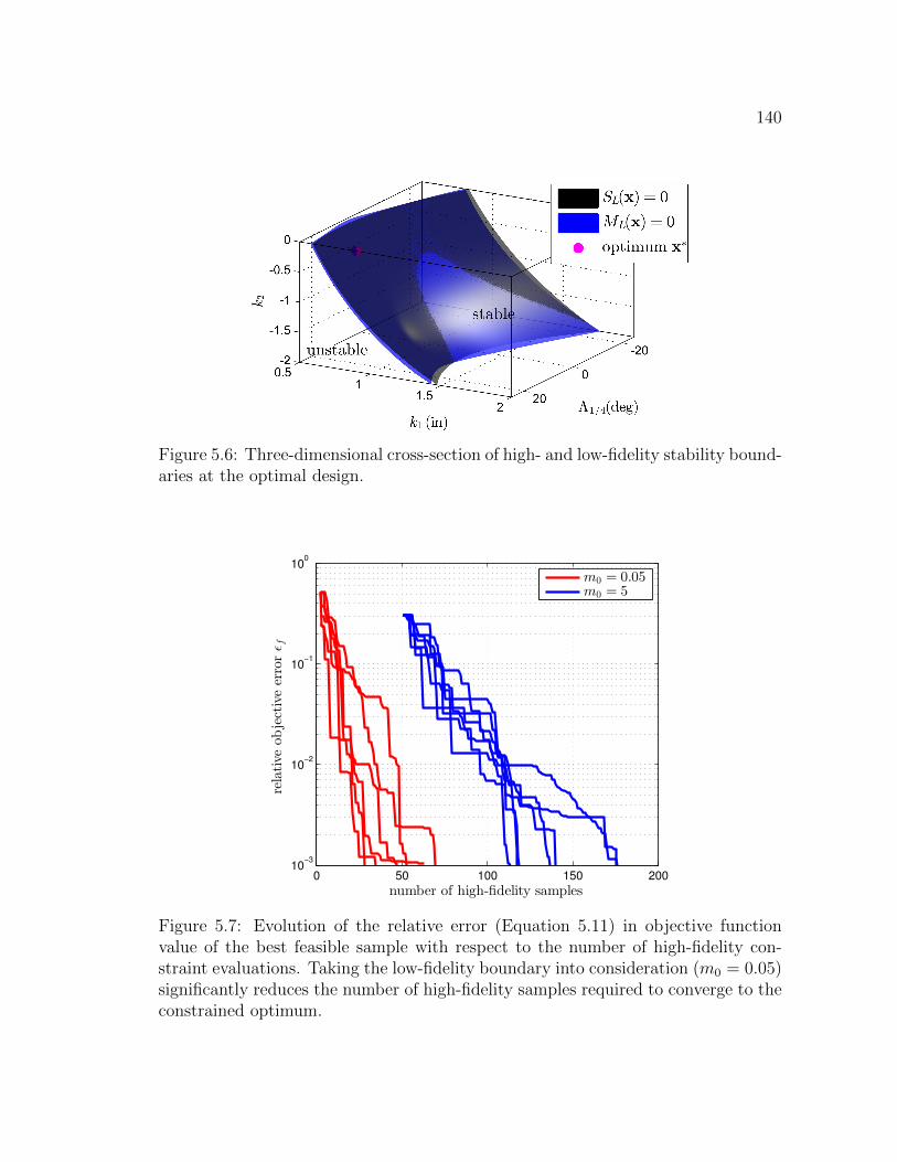
140

Figure 5.6: Three-dimensional cross-section of high- and low-fidelity stability bound-aries at the optimal design.

0 50 100 150 20010

−3

10−2

10−1

100

number of high-fidelity samples

relativeobjectiveerrorǫf

m0 = 0.05m0 = 5

Figure 5.7: Evolution of the relative error (Equation 5.11) in objective functionvalue of the best feasible sample with respect to the number of high-fidelity con-straint evaluations. Taking the low-fidelity boundary into consideration (m0 = 0.05)significantly reduces the number of high-fidelity samples required to converge to theconstrained optimum.

141

CHAPTER 6

CONCLUSIONS

This chapter summarizes the conclusions on the proposed multi-fidelity algorithm

and discusses its limitations to show opportunities for future improvements and

extensions.

The multi-fidelity algorithm proposed in Chapter 3 enables the user to construct

a support vector machine predictor (SVM) of design failure. To minimize simula-

tion costs, training samples are selected iteratively and the algorithm chooses one

of two levels of fidelity for each evaluation. Thereby, it addresses the challenges

presented by design constraints that are expensive to evaluate and not effectively

approximated by traditional meta-models due to discontinuous simulation responses.

Further, since the SVM training process is based only on the classification of train-

ing samples as feasible or infeasible, it does not distinguish between various failure

modes and therefore a single SVM may represent multiple design constraints. The

resulting SVM function is an analytical, differentiable expression ideally suited for

computational design methods, such as numerical optimization and reliability quan-

tification.

The multi-fidelity algorithm is tested on various analytical test problems (Sec-

tions 3.4) as well as two simulation models to predict aeroelastic stability (Section

4). While the analytical problems are designed to study the performance of the

algorithm in detail, the aeroelasticity models demonstrate the applicability of the

algorithm to realistic engineering problems. It is found that the prediction error

of the SVM constructed by the algorithm reliably converges towards zero as train-

ing samples are added iteratively. Specifically, the convergence is approximately

exponential while the rate of convergence is problem dependent. The multi-fidelity

algorithm takes advantage of a low-fidelity boundary to classify some of the SVM

training samples and the test problems show that this multi-fidelity approach re-

142

duces the overall computational burden. The benefit of the multi-fidelity approach

in terms of reducing the overall cost depends both of the accuracy of the low-fidelity

boundary and the cost of obtaining it. For cases where the low-fidelity boundary

represents a good approximation of the high-fidelity constraint model, the com-

putational savings ranged from 10 to 60%. In addition, the third analytical test

problem (Section 3.4) suggests that the benefit increases with the dimensionality of

the design problem. On the other hand, the second analytical test problem (Sec-

tion 3.4) demonstrates that even if the low-fidelity boundary is very inaccurate and

therefore misleading to the multi-fidelity algorithm, the resulting penalty in terms

of computational efficiency is small.

Chapter 5 presents a variant of the multi-fidelity algorithm specifically geared

towards numerical design optimization that limits simulations to regions of the de-

sign space with the potential to improve on the current best, feasible design. The

usefulness of this algorithm variant is limited to relatively low-dimensional optimiza-

tion problems where the computational cost of the objective function is negligible

compared to the evaluation cost of the constraints. However, for this sub-set of

problems the efficiency of the algorithm is demonstrated both on analytical test

problems and on the optimization of a cantilevered wing in terms of five geometrical

parameters. Here the structural weight is minimized while satisfying an aeroelas-

tic stability constraint and the convergence towards the constrained optimum is

approximately exponential.

Several limitations of the algorithm present opportunities for future improve-

ments. For example, it is assumed that the high-fidelity constraint model classifies

samples consistently such that feasible and infeasible samples may be separated en-

tirely by an SVM boundary. This assumption is generally justified in the case of

simulation models, but if experimental data is incorporated, there might be several

sources of uncertainty. This leads to non-separable data sets, where the best SVM

approximation of the true boundary misclassifies some of the samples. Adapting

the multi-fidelity algorithm for such a scenario would require major modifications

to how assumptions on the accuracy of the low-fidelity boundary are generated and

143

how the SVM is constructed (Section 3.3.5).

In addition, the algorithm is not suited for very high-dimensional problems with,

for example, hundreds of variables. This limitation is due to the large role of Eu-

clidean distance in the iterative selection of training samples in the design space

and also for the selection of fidelity levels. With increasing dimensionality, more

and more adaptive samples would be located on the boundary of the design space,

and convergence of the SVM to the actual boundary of the feasible space would likely

to be very slow. However, with a different criterion for the selection of samples, the

multi-fidelity approach may well be applicable to such problems.

144

REFERENCES

Abe, S. (2010). Support Vector Machines for Pattern Classification. Springer.

Aizerman, A., E. Braverman, and L. Rozoner (1964). Theoretical Foundations ofthe Potential Function Method in Pattern Recognition Learning. Automation andremote control, 25, pp. 821–837.

Alexandrov, N., J. Dennis, R. Lewis, and V. Torczon (1998). A Trust-Region Frame-work for Managing the Use of Approximation Models in Optimization. Structuraland Multidisciplinary Optimization, 15(1), pp. 16–23. doi:10.1007/BF01197433.

Alexandrov, N., R. Lewis, C. Gumbert, L. Green, and P. Newman (2001). Approx-imation and Model Management in Aerodynamic Optimization with Variable-Fidelity Models. Journal of Aircraft, 38(6), pp. 1093–1101.

Alexandrov, N. M., E. J. Nielsen, R. M. Lewis, and W. K. Anderson (2000).First-Order Model Management With Variable-Fidelity Physics Applied to Multi-Element Airfoil Optimization. Technical report, Nasa Langley Research Center.

Alpaydin, E. (2004). Introduction to Machine Learning. The MIT Press. ISBN0262012111.

Antoine, C. and J. Kergomard (2008). Acoustique des Instruments de Musique.Belin.

Balabanov, V., R. T. Haftka, B. Grossman, W. H. Mason, and L. T. Watson (1998).Multifidelity Response Surface Model for HSCT Wing Bending Material Weight.In 7th AIAA/USAF/NASA/ISSMO Symposium on Multidisciplinary Analysisand Optimization, AIAA–1998–4804, pp. 778–788.

Balabanov, V. and G. Venter (2004). Multi-Fidelity Optimization with High-FidelityAnalysis and Low-Fidelity Gradients. In 10 th AIAA/ISSMO MultidisciplinaryAnalysis and Optimization Conference.

Bandler, J., Q. Cheng, S. Dakroury, A. Mohamed, M. Bakr, K. Madsen, and J. Son-dergaard (2004). Space Mapping: The State of the Art. Microwave Theory andTechniques, IEEE Transactions on, 52(1), pp. 337–361.

Barakat, N. and A. P. Bradley (2010). Rule Extraction from Support Vector Ma-chines: A Review. Neurocomputing, 74(13), pp. 178 – 190. ISSN 0925-2312.doi:10.1016/j.neucom.2010.02.016. ¡ce:title¿Artificial Brains¡/ce:title¿.

145

Basudhar, A. (2012). Computational Optimal Design and Uncertainty Quantifica-tion of Complex Systems Using Explicit Decision Boundaries. Ph.D. thesis, TheUniversity of Arizona.

Basudhar, A., C. Dribusch, S. Lacaze, and S. Missoum (2012). Constrained Ef-ficient Global Optimization with Support Vector Machines. Structural andMultidisciplinary Optimization, 46(2), pp. 201–221. ISSN 1615-147X. doi:10.1007/s00158-011-0745-5. 10.1007/s00158-011-0745-5.

Basudhar, A. and S. Missoum (2010). An Improved Adaptive Sampling Schemefor the Construction of Explicit Boundaries. Structural and MultidisciplinaryOptimization, 42, pp. 517–529. ISSN 1615-147X. doi:10.1007/s00158-010-0511-0.10.1007/s00158-010-0511-0.

Basudhar, A., S. Missoum, and S. Harrison (2008). Limit State Function Identifi-cation Using Support Vector Machines for Discontinuous Responses and DisjointFailure Domains. Probabilistic Engineering Mechanics, 23(1), pp. 1–11. ISSN0266-8920. doi:10.1016/j.probengmech.2007.08.004.

Bennett, K. and C. Campbell (2000). Support Vector Machines: Hype or Hallelujah?ACM SIGKDD Explorations Newsletter, 2(2), pp. 1–13.

Beran, P., T. Strganac, K. Kim, and C. Nichkawde (2004). Studies of Store-InducedLimit-Cycle Oscillations Using a Model with Full System Nonlinearities. NonlinearDynamics, 37(4), pp. 323–339.

Berci, M., P. H. Gaskell, R. W. Hewson, and V. V. Toropov (2011). Multi-fidelity Metamodel Building as a Route to Aeroelastic Optimization of Flex-ible Wings. Proceedings of the Institution of Mechanical Engineers, PartC: Journal of Mechanical Engineering Science, 225(9), pp. 2115–2137. doi:10.1177/0954406211403549.

Berci, M., V. V. Toropov, R. W. Hewson, and P. Gaskell (2009). MetamodellingBased on High and Low Fidelity Model Interaction for UAV Gust PerformanceOptimization. In 50th AIAA/ASME/ASCE/AHS/ASC Structures, StructuralDynamics, and Materials Conference, AIAA–2009–2215. AIAA, AIAA.

Bhatia, K. G. (2003). Airplane Aeroelasticity: Practice and Potential. Journal ofAircraft, 40(6), pp. 1010–1018.

Bisplinghoff, R. L., H. Ashley, and R. L. Halfman (1962). Aeroelasticity. Dover,New York.

Boser, B., I. Guyon, and V. Vapnik (1992). A Training Algorithm for OptimalMargin Classifiers. In Proceedings of the fifth annual workshop on Computationallearning theory, pp. 144–152. ACM.

146

Box, G. E. P. and N. R. Draper (1987). Empirical Model-Building and ResponseSurfaces (Wiley Series in Probability and Statistics). John Wiley & Sons, NewYork. ISBN 0471810339.

Broomhead, D. and D. Lowe (1988). Multivariable Functional Interpolation andAdaptive Networks. Complex systems, 2, pp. 321–355.

Byun, H. and S. Lee (2002). Applications of Support Vector Machines for PatternRecognition: A Survey. Pattern recognition with support vector machines, pp.571–591.

Carpenter, J. and J. Bithell (2000). Bootstrap Confidence Intervals: When, Which,What? A Practical Guide for Medical Statisticians. Statistics in medicine, 19(9),pp. 1141–1164.

Chang, C.-C. and C.-J. Lin (2011). LIBSVM: A Library for Support Vector Ma-chines. ACM Trans. Intell. Syst. Technol., 2(3), pp. 27:1–27:27. ISSN 2157-6904.doi:10.1145/1961189.1961199.

Chang, K. J., G. L. Giles, R. T. Haftka, and P.-J. Kao (1993). Sensitivity-BasedScaling for Approximating Structural Response. Journal of Aircraft, 30(2), pp.283–288. ISSN 0021-8669. doi:10.2514/3.48278.

Chapelle, O., V. Vapnik, O. Bousquet, and S. Mukherjee (2002). Choosing MultipleParameters for Support Vector Machines. Machine Learning, 46, pp. 131–159.ISSN 0885-6125. 10.1023/A:1012450327387.

Chen, P. (2000). Damping Perturbation Method for Flutter Solution: The G-Method. AIAA journal, 38(9), pp. 1519–1524.

Clarke, S. M., J. H. Griebsch, and T. W. Simpson (2005). Analysis of SupportVector Regression for Approximation of Complex Engineering Analyses. Journalof Mechanical Design, 127(6), pp. 1077–1087. doi:10.1115/1.1897403.

Cressie, N. (1990). The Origins of Kriging. Mathematical Geology, 22, pp. 239–252.ISSN 0882-8121. 10.1007/BF00889887.

Cressie, N. (1993). Statistics for Spatial Data. Wiley series in probability andmathematical statistics: Applied probability and statistics. J. Wiley, 2 edition.ISBN 9780471002550.

Cristianini, N. and B. Scholkopf (2002). Support Vector Machines and Kernel Meth-ods: The New Generation of Learning Machines. Artificial Intelligence Magazine,23(3), pp. 31–41.

147

Den Hertog, D., J. Kleijnen, and A. Siem (2005). The Correct Kriging VarianceEstimated by Bootstrapping. Journal of the Operational Research Society, 57(4),pp. 400–409.

Dixon, L. (1978). Towards Global Optimisation 2. Towards Global Optimisation.North-Holland Pub. Co. ISBN 9780444851710.

Dowell, E. and D. Tang (2002). Nonlinear Aeroelasticity and Unsteady Aerodynam-ics. AIAA Journal, 40(9), pp. 1697–1707. doi:10.2514/2.1853.

Du, Q., V. Faber, and M. Gunzburger (1999). Centroidal Voronoi Tessellations: Ap-plications and Algorithms. SIAM Review, 41(4), pp. pp. 637–676. ISSN 00361445.

Duch, W. and N. Jankowski (1999). Survey of Neural Transfer Functions. NeuralComputing Surveys, 2(1), pp. 163–212.

Efron, B. (1983). Estimating the Error Rate of a Prediction Rule: Improvement onCross-Validation. Journal of the American Statistical Association, pp. 316–331.

Efron, B. and R. Tibshirani (1993). An Introduction to the Bootstrap, volume 57.Chapman & Hall/CRC.

Eldred, M. S. and D. M. Dunlavy (2006). Formulations for Surrogate-Based Op-timization with Data-Fit, Multifidelity and Reduced-Order Models. In 11 thAIAA/ISSMO Multidisciplinary Analysis and Optimization Conference, AIAA–2006–7117. AIAA, AIAA.

Eldred, M. S., A. A. Giunta, S. S. Collis, N. A. Alexandrov, and R. M. Lewis(2004). Second-Order Corrections for Surrogate-Based Optimization with ModelHierarchies. In Proceedings of the 10th AIAA/ISSMO Multidisciplinary Analysisand Optimization Conference, 4457.

Fish, J. and T. Belytschko (2007). A First Course in Finite Elements. John Wiley& Sons. ISBN 9780470035801.

Floudas, C. and C. Gounaris (2009). A Review of Recent Advances in GlobalOptimization. Journal of Global Optimization, 45, pp. 3–38. ISSN 0925-5001.10.1007/s10898-008-9332-8.

Forrester, A. and D. Jones (2008). Global optimization of Deceptive Functions withSparse Sampling. In 12th AIAA/ISSMO multidisciplinary analysis and optimiza-tion conference, Victoria, British Columbia, Canada, pp. 10–12.

Forrester, A. I. and A. J. Keane (2009). Recent Advances in Surrogate-Based Opti-mization. Progress in Aerospace Sciences, 45(1-3), pp. 50 – 79. ISSN 0376-0421.doi:10.1016/j.paerosci.2008.11.001.

148

Friedman, J., T. Hastie, and R. Tibshirani (2001). The Elements of StatisticalLearning, volume 1. Springer Series in Statistics.

Fung, Y. (2002). An Introduction to the Theory of Aeroelasticity. Courier DoverPublications.

Furey, T., N. Cristianini, N. Duffy, D. Bednarski, M. Schummer, and D. Haussler(2000). Support Vector Machine Classification and Validation of Cancer TissueSamples using Microarray Expression Data. Bioinformatics, 16(10), pp. 906–914.

Gano, S., J. Renaud, J. Martin, and T. Simpson (2006). Update Strategies forKriging Models Used in Variable Fidelity Optimization. Structural and Multidis-ciplinary Optimization, 32(4), pp. 287–298. doi:10.1007/s00158-006-0025-y.

Gano, S., J. Renaud, and B. Sanders (2005). Hybrid Variable Fidelity Optimizationby Using a Kriging-Based Scaling Function. AIAA Journal, 43(11), pp. 2422–2433. doi:10.2514/1.12466.

Gibbs, M. (1997). Bayesian Gaussian Processes for Regression and Classification.Ph.D. thesis, Citeseer.

Giunta, A., V. Balabanov, M. Kaufman, S. Burgee, B. Grossman, R. Haftka, W. Ma-son, and L. Watson (1995a). Variable-Complexity Response Surface Design of anHSCT Configuration. In Proceedings of ICASE/LaRC Workshop on Multidisci-plinary Design Optimization, Hampton, VA.

Giunta, A., R. Narducci, S. Burgee, B. Grossman, W. Mason, L. Watson, andR. Haftka (1995b). Variable-Complexity Response Surface Aerodynamic Designof an HSCT Wing. In 13th AIAA Applied Aerodynamics Conference, AIAA–1995–1886. AIAA, AIAA.

Glaz, B., T. Goel, L. Liu, P. Friedmann, and R. Haftka (2009). Multiple-SurrogateApproach to Helicopter Rotor Blade Vibration Reduction. AIAA Journal, 47,pp. 271–282. doi:10.2514/1.40291.

Goel, T., R. Haftka, W. Shyy, and N. Queipo (2007). Ensemble of Surrogates.Structural and Multidisciplinary Optimization, 33, pp. 199–216. ISSN 1615-147X.10.1007/s00158-006-0051-9.

Gunn, S. (1998). Support Vector Machines for Classification and Regression. Tech-nical report, University of Southampton.

Gutmann, H.-M. (2001). A Radial Basis Function Method for Global Optimization.Journal of Global Optimization, 19, pp. 201–227. ISSN 0925-5001. doi:10.1023/A:1011255519438. 10.1023/A:1011255519438.

149

Guzella, T. S. and W. M. Caminhas (2009). A Review of Machine Learning Ap-proaches to Spam Filtering. Expert Systems with Applications, 36(7), pp. 10206– 10222. ISSN 0957-4174. doi:10.1016/j.eswa.2009.02.037.

Haftka, R. T. (1991). Combining Global and Local Approximations. AIAA Journal,29(9), pp. 1523–1525.

Haldar, A. and S. Mahadevan (2000). Probability, Reliability, and Statistical Meth-ods in Engineering Design. John Wiley. ISBN 9780471331193.

Hall, P. (1986). On the Bootstrap and Confidence Intervals. The Annals of Statistics,14(4), pp. pp. 1431–1452. ISSN 00905364.

Hodges, D. and G. Pierce (2011). Introduction to Structural Dynamics and Aeroe-lasticity. Cambridge Aerospace Series. Cambridge University Press. ISBN9780521195904.

Hodges, D. H. (2012). Book Review: Theoretical and Computational Aeroelasticity.Journal of Aircraft, 50(4), pp. 990–991. doi:10.2514/1.J051738.

Huber, P. (1964). Robust Estimation of a Location Parameter. The Annals ofMathematical Statistics, 35(1), pp. 73–101.

Hutchison, M. G., B. Grossman, R. T. Haftka, W. H. Mason, and E. R. Unger(1994). Variable-Complexity Aerodynamic Optimization of a High-Speed CivilTransport Wing. Journal of Aircraft, 31(1), pp. 110–116. ISSN 0021-8669. doi:10.2514/3.46462.

Irwin, C. and P. Guyett (1965). The Subcritical Response and Flutter of a Swept-Wing Model. Technical Report 3497, United Kingdom Ministry of Technology,Aeronautical Research Council.

Joachims, T. (1998). Text Categorization With Support Vector Machines: LearningWith Many Relevant Features. Machine learning: ECML-98, pp. 137–142.

Jones, D. (2001). A Taxonomy of Global Optimization Methods Based on ResponseSurfaces. Journal of Global Optimization, 21(4), pp. 345–383.

Jones, D., M. Schonlau, and W. Welch (1998). Efficient Global Optimization ofExpensive Black-Box Functions. Journal of Global optimization, 13(4), pp. 455–492.

Karlsen, R., D. Gorsich, and G. Gehart (2000). Target Classification Via SupportVector Machines. Optical Engineering, 39(3), pp. 704–711. doi:10.1117/1.602417.

150

Karush, W. (1939). Minima of Functions of Several Variables with Inequalities asSide Constraints. Master’s thesis, Dept. of Mathematics, Univ. of Chicago.

Kaufman, M., V. Balabanov, A. A. Giunta, B. Grossman, W. H. Mason, S. L.Burgee, R. T. Haftka, and L. T. Watson (1996). Variable-Complexity ResponseSurface Approximations for Wing Structural Weight in HSCT Design. Computa-tional Mechanics, 18(2), pp. 112–126. doi:10.1007/BF00350530.

Keane, A. (2003). Wing Optimization Using Design of Experiment, Response Sur-face, and Data Fusion Methods. Journal of Aircraft, 40(4), pp. 741–750.

Keane, A. and P. Nair (2005). Computational Approaches for Aerospace Design.Wiley Online Library. doi:10.1002/0470855487.fmatter.

Kleijnen, J. (2009). Kriging Metamodeling in Simulation: A Review. EuropeanJournal of Operational Research, 192(3), pp. 707–716.

Kleijnen, J., W. van Beers, and I. van Nieuwenhuyse (2012). Expected Improve-ment in Efficient Global Optimization Through Bootstrapped Kriging. Journal ofGlobal Optimization, 54, pp. 59–73. ISSN 0925-5001. 10.1007/s10898-011-9741-y.

Knill, D. L., A. A. Giunta, C. A. Baker, B. Grossman, W. H. Mason, R. T. Haftka,and L. T. Watson (1998). HSCT Configuration Design Using Response SurfaceApproximations of Supersonic Euler Aerodynamics. In 36th Aerospace SciencesMeeting and Exhibit, AIAA-1998-0905. AIAA, AIAA.

Koehler, J. and A. Owen (1996). Computer Experiments. Handbook of statistics,13(13), pp. 261–308.

Kousen, K. and O. Bendiksen (1994). Limit Cycle Phenomena in ComputationalTransonic Aeroelasticity. Journal of Aircraft, 31(6), pp. 1257–1263. doi:10.2514/3.46644.

Koziel, S., Q. Cheng, and J. Bandler (2008). Space Mapping. Microwave Magazine,IEEE, 9(6), pp. 105 –122. ISSN 1527-3342. doi:10.1109/MMM.2008.929554.

Krige, D. G. (1951). A Statistical Approach to Some Basic Mine Valuation Problemson the Witwatersrand. Journal of the Chemcial, Metallurgical and Mining Societyof South Africa, 52, pp. 119–139.

Kuhn, H. W. and A. W. Tucker (1951). Nonlinear Programming. In Second Berkeleysymposium on mathematical statistics and probability, volume 1, pp. 481–492.

Lachenbruch, P. and M. Mickey (1968). Estimation of Error Rates in DiscriminantAnalysis. Technometrics, pp. 1–11.

151

Leary, S. J., A. Bhaskar, and A. J. Keane (2003). A Knowledge-Based ApproachTo Response Surface Modelling in Multifidelity Optimization. Journal of GlobalOptimization, 26(3), pp. 297–319. doi:10.1023/A:1023283917997.

Lee, B., L. Jiang, and Y. Wong (1999a). Flutter of an Airfoil with Cubic RestoringForce. Journal of Fluids and Structures, 13(1), pp. 75–101. doi:10.1006/jfls.1998.0190.

Lee, B., S. Price, and Y. Wong (1999b). Nonlinear Aeroelastic Analysis of Airfoils:Bifurcation and Chaos. Progress in Aerospace Sciences, 35(3), pp. 205–334. doi:10.1016/S0376-0421(98)00015-3.

Li, H., Y. Liang, and Q. Xu (2009). Support Vector Machines and Its Applicationsin Chemistry. Chemometrics and Intelligent Laboratory Systems, 95(2), pp. 188–198.

Lloyd, S. (1982). Least Squares Quantization in PCM. Information Theory, IEEETransactions on, 28(2), pp. 129 – 137. ISSN 0018-9448. doi:10.1109/TIT.1982.1056489.

Martin, J. and T. Simpson (2005). Use of Kriging Models to Approximate Deter-ministic Computer Models. AIAA journal, 43(4), pp. 853–863.

McKay, M., R. Beckman, and W. Conover (1979). A Comparison of Three Methodsfor Selecting Values of Input Variables in the Analysis of Output from a ComputerCode. Technometrics, pp. 239–245.

Min, J. and Y. Lee (2005). Bankruptcy Prediction Using Support Vector Machinewith Optimal Choice of Kernel Function Parameters. Expert systems with appli-cations, 28(4), pp. 603–614.

Missoum, S., C. Dribusch, and P. Beran (2010). Reliability-Based Design Opti-mization of Nonlinear Aeroelasticity Problems. Journal of Aircraft, 47(3), pp.992–998. doi:10.2514/1.46665.

Mohandes, M., T. Halawani, S. Rehman, and A. A. Hussain (2004). Support VectorMachines for Wind Speed Prediction. Renewable Energy, 29(6), pp. 939 – 947.ISSN 0960-1481. doi:10.1016/j.renene.2003.11.009.

Mountrakis, G., J. Im, and C. Ogole (2011). Support Vector Machines in RemoteSensing: A Review. ISPRS Journal of Photogrammetry and Remote Sensing,66(3), pp. 247–259.

Myers, R., D. Montgomery, and C. Anderson-Cook (2009). Response SurfaceMethodology: Process and Product Optimization Using Designed Experiments,volume 705. John Wiley & Sons Inc.

152

Myers, R. H. and D. C. Montgomery (1995). Response Surface Methodology: Pro-cess and Product Optimization Using Designed Experiments. Wiley-Interscience,1 edition.

Nocedal, J. and S. Wright (2006). Numerical Optimization. Springer series inoperations research. Springer. ISBN 9780387303031.

Noll, T., J. Brown, M. Perez-Davis, S. Ishmael, G. Tiffany, and M. Gaier (2004).Investigation of the Helios Prototype Aircraft Mishap Volume I Mishap Report.Technical report, NASA.

Okabe, A., B. Boots, K. Sugihara, and S. Chiu (1992). Spatial Tessellations: Con-cepts and Applications of Voronoi Diagrams. Wiley & Sons Chichester.

Orr, G., W. Pettersson-Yeo, A. F. Marquand, G. Sartori, and A. Mechelli (2012).Using Support Vector Machine to Identify Imaging Biomarkers of Neurologicaland Psychiatric Disease: A Critical Review. Neuroscience &amp; BiobehavioralReviews, 36(4), pp. 1140 – 1152. ISSN 0149-7634. doi:10.1016/j.neubiorev.2012.01.004.

Parr, J. M., A. J. Keane, A. I. Forrester, and C. M. Holden (2012). Infill SamplingCriteria for Surrogate-Based Optimization with Constraint Handling. EngineeringOptimization, 0(0), pp. 1–20. doi:10.1080/0305215X.2011.637556.

Patil, M., D. Hodges, and C. Cesnik (2001). Limit-Cycle Oscillations in High AspectRatio Wings. Journal of Fluids and Structures, 15(1), pp. 107–132.

Plackett, R. and J. Burman (1946). The Design of Optimum Multifactorial Exper-iments. Biometrika, 33(4), pp. 305–325.

Queipo, N., R. Haftka, W. Shyy, T. Goel, R. Vaidyanathan, and P. Kevin Tucker(2005). Surrogate-Based Analysis and Optimization. Progress in Aerospace Sci-ences, 41(1), pp. 1–28. doi:10.1016/j.paerosci.2005.02.001.

Ralston, A. and P. Rabinowitz (1978). A first Course in Numerical Analy-sis. International series in pure and applied mathematics. McGraw-Hill. ISBN9780070511583.

Redhe, M. and L. Nilsson (2006). A Multipoint Version of Space Mapping Optimiza-tion Applied to Vehicle Crashworthiness Design. Structural and MultidisciplinaryOptimization, 31, pp. 134–146. ISSN 1615-147X. 10.1007/s00158-005-0544-y.

Robinson, T. (2007). Surrogate-Based Optimization Using Multifidelity Models withVariable Parameterization. Ph.D. thesis, Massachusetts Institute of Technology.

153

Robinson, T., M. Eldred, K. Willcox, and R. Haimes (2006a). Strategies for Multifi-delity Optimization with Variable Dimensional Hierarchical Models. In Proceed-ings of the 47th AIAA/ASME/ASCE/AHS/ASC Structures, Structural Dynam-ics, and Materials Conference (2nd AIAA Multidisciplinary Design OptimizationSpecialist Conference), Newport, RI, pp. 2006–1819.

Robinson, T., M. Eldred, K. Willcox, and R. Haimes (2008). Surrogate-Based Op-timization Using Multifidelity Models with Variable Parameterization and Cor-rected Space Mapping. Aiaa Journal, 46(11), pp. 2814–2822.

Robinson, T., K. Willcox, M. Eldred, and R. Haimes (2006b). Multifidelity Op-timization for Variable-Complexity Design. In 11th AIAA/ISSMO Multidisci-plinary Analysis and Optimization Conference, AIAA–2006–7114. AIAA, AIAA.

Rodden, W. (2011). Theoretical and Computational Aeroelasticity. Crest Publish-ing. ISBN 9780692012413.

Rodden, W. and E. Johnson (1994). MSC/NASTRAN Aeroelastic Analysis: User’sGuide, Version 68. MacNeal-Schwendler Corporation.

Rodden, W. and J. Love (1985). Equations of Motion of a Quasisteady Flight VehicleUtilizing Restrained Static Aeroelastic Characteristics. Journal of Aircraft, 22(9),pp. 802–809. doi:10.2514/3.45205.

Rodden, W. P., R. L. Harder, and E. D. Bellinger (1979). Aeroelastic Addition toNastran. Technical Report 3094, NASA.

Sacks, J., S. Schiller, and W. Welch (1989a). Designs for Computer Experiments.Technometrics, pp. 41–47.

Sacks, J., W. Welch, T. Mitchell, and H. Wynn (1989b). Design and Analysis ofComputer Experiments. Statistical science, 4(4), pp. 409–423.

Saijal, K., R. Ganguli, and S. Viswamurthy (2011). Optimization of HelicopterRotor Using Polynomial and Neural Network Metamodels. Journal of Aircraft,48(2), pp. 553–566. doi:10.2514/1.53495.

Sasena, M. J. (2002). Flexibility and Efficiency Enhancements for ConstrainedGlobal Design Optimization with Kriging Approximations. Ph.D. thesis, Citeseer.

Scholkopf, B., C. J. C. Burges, and A. J. Smola (eds.) (1998). Advances in KernelMethods. The MIT Press.

Scholkopf, B. and A. Smola (2001). Learning with Kernels: Support Vector Ma-chines, Regularization, Optimization, and Beyond. MIT press.

154

Scholkopf, B., K.-K. Sung, C. Burges, F. Girosi, P. Niyogi, T. Poggio, and V. Vapnik(1997). Comparing Support Vector Machines with Gaussian Kernels to RadialBasis Function Classifiers. Signal Processing, IEEE Transactions on, 45(11), pp.2758 –2765. ISSN 1053-587X. doi:10.1109/78.650102.

Schuster, D. M., D. D. Liu, and L. J. Huttsell (2003). Computational Aeroelasticity:Success, Progress, Challenge. Journal of Aircraft, 40(5), pp. 843–856. doi:10.2514/2.6875.

Seydel, R. (1988). From Equilibrium to Chaos: Practical Bifurcation and StabilityAnalysis. Elsevier Science Ltd.

Simpson, T., J. Poplinski, P. N. Koch, and J. Allen (2001). Metamodels forComputer-Based Engineering Design: Survey and Recommendations. Engineer-ing with Computers, 17, pp. 129–150. ISSN 0177-0667. 10.1007/PL00007198.

Sobester, A. (2003). Enhancements to Global Design Optimization Techniques.Ph.D. thesis, University of Southampton.

Stone, M. (1974). Cross-Validatory Choice and Assessment of Statistical Predictions.Journal of the Royal Statistical Society. Series B (Methodological), 36(2), pp. pp.111–147. ISSN 00359246.

Swiler, L., R. Slepoy, and A. Giunta (2006). Evaluation of Sampling Meth-ods in Constructing Response Surface Approximations. In Proc. 47thAIAA/ASME/ASCE/AHS/ASC Structures, Structural Dynamics, and Materi-als Conference, number AIAA-2006-1827, Newport, RI.

Theodorson, T. (1935). General Theory of Aerodynamic Instability and the Mech-anism of Flutter. Technical Report 496, National Advisory Commitee for Aero-nautics.

Toropov, V., V. Markine, P. Meijers, and J. Meijaard (1997). Optimization of a Dy-namic System Using Multipoint Approximations and Simplified Numerical Model.In Proceedings of the Second World Congress of Structural and MultidisciplinaryOptimization, pp. 613–618. Polish Academy of Sciences.

Toropov, V. V. and E. Van der Giessen (1993). Parameter Identification for Non-linear Constitutive Models: Finite Element Simulation–Optimization–NontrivialExperiments. In Pedersen, P. (ed.) Proceedings of IUTAM Symposium on Opti-mal Design of Advanced Materials, The Frithiof I. Niordson Volume, pp. 113–130.IUTAM, Elesevier Scientific Publishers, Amsterdam.

Unger, E., M. Hutchinson, X. Huang, W. Mason, R. Haftka, and B. Grossmann(1992). Variable-Complexity Aerodynamic-Structural Design of a High-Speed

155

Civil Transport. In 4th AIAA/NASA/USAF/OAI Symposium on Multidisci-plinary Analysis and Optimization, AIAA–1992–4695. AIAA, AIAA.

Vanderplaats (2006). Genesis Analysis Manual Version 9.0. Vanderplaats Research& Developement, Inc.

Vanderplaats, G. (2005). Numerical Optimization Techniques for Engineering De-sign. Vanderplaats Research & Development, Incorporated. ISBN 9780944956021.

Vapnik, V. (1963). Pattern Recognition Using Generalized Portrait Method. Au-tomation and Remote Control, 24, pp. 774–780.

Vapnik, V. (1995). The Nature of Statistical Learning Theory. Springer-Verlag NewYork Inc.

Vapnik, V. (1998). Statistical Learning Theory. Adaptive and learning systems forsignal processing, communications, and control. Wiley. ISBN 9780471030034.

Vapnik, V., S. Golowich, and A. Smola (1996). Support Vector Method for FunctionApproximation, Regression Estimation, and Signal Processing. In Advances inNeural Information Processing Systems 9. Citeseer.

Viana, F. (2011). Multiple Surrogates for Prediction and Optimization. Ph.D. thesis,University of Florida.

Viana, F., R. Haftka, and V. Steffen (2009). Multiple Surrogates: How Cross-Validation Errors Can Help Us to Obtain the Best Predictor. Structural and Mul-tidisciplinary Optimization, 39, pp. 439–457. ISSN 1615-147X. 10.1007/s00158-008-0338-0.

Viana, F. A. C., G. Venter, and V. Balabanov (2010). An Algorithm for Fast OptimalLatin Hypercube Design of Experiments. International Journal for NumericalMethods in Engineering, 82(2), pp. 135–156. ISSN 1097-0207. doi:10.1002/nme.2750.

Voronoi, G. (1908). Nouvelles Applications des Paramtres Continus la Thoriedes Formes Quadratiques. Premier Mmoire. Sur Quelques Proprits des FormesQuadratiques Positives Parfaites. Journal fr die reine und angewandte Mathe-matik (Crelle’s Journal), 1908(133), pp. 97–102. doi:10.1515/crll.1908.133.97.

Welch, W., R. J. Buck, J. Sacks, H. Wynn, T. Mitchell, and M. Morris (1992).Screening, Predicting, and Computer Experiments. Technometrics, pp. 15–25.

Welch, W., T. Yu, S. Kang, and J. Sacks (1990). Computer Experiments for QualityControl by Parameter Design. Journal of Quality Technology, 22(1), pp. 15–15.

156

Wolfe, P. (1961). A Duality Theorem for Nonlinear Programming. Quarterly ofapplied mathematics, 19(3), pp. 239–244.

Wright, J. and J. Cooper (2007). Introduction to Aircraft Aeroelasticity and Loads.Aerospace Series. John Wiley & Sons. ISBN 9780470858400.

Ye, K., W. Li, and A. Sudjianto (2000). Algorithmic Construction of OptimalSymmetric Latin Hypercube Designs. Journal of statistical planning and inference,90(1), pp. 145–159. doi:10.1016/S0378-3758(00)00105-1.

Zien, A., G. Rtsch, S. Mika, B. Schlkopf, T. Lengauer, and K.-R. Mller (2000). En-gineering Support Vector Machine Kernels That Recognize Translation InitiationSites. Bioinformatics, 16(9), pp. 799–807. doi:10.1093/bioinformatics/16.9.799.

Zona (2011). ZAERO Theoretical Manual Version 8.5. ZONA Technology Inc, 21stedition.