Multi-Criteria Dimensionality Reduction withApplications to Fairness

Uthaipon (Tao) Tantipongpipat∗ Samira Samadi∗ Mohit Singh∗

Jamie Morgenstern† Santosh Vempala∗

June 17, 2020

Abstract

Dimensionality reduction is a classical technique widely used for data analysis. One foundationalinstantiation is Principal Component Analysis (PCA), which minimizes the average reconstruction error.In this paper, we introduce the multi-criteria dimensionality reduction problem where we are givenmultiple objectives that need to be optimized simultaneously. As an application, our model capturesseveral fairness criteria for dimensionality reduction such as our novel Fair-PCA problem and the NashSocial Welfare (NSW) problem. In Fair-PCA, the input data is divided into k groups, and the goal is tofind a single d-dimensional representation for all groups for which the minimum variance of any onegroup is maximized. In NSW, the goal is to maximize the product of the individual variances of thegroups achieved by the common low-dimensional space.

Our main result is an exact polynomial-time algorithm for the two-criterion dimensionality reductionproblem when the two criteria are increasing concave functions. As an application of this result, we obtaina polynomial time algorithm for Fair-PCA for k = 2 groups and a polynomial time algorithm for NSWobjective for k = 2 groups. We also give approximation algorithms for k > 2. Our technical contributionin the above results is to prove new low-rank properties of extreme point solutions to semi-definiteprograms. We conclude with experiments indicating the effectiveness of algorithms based on extremepoint solutions of semi-definite programs on several real-world data sets.

1 Introduction

Dimensionality reduction is the process of choosing a low-dimensional representation of a large, high-dimensional data set. It is a core primitive for modern machine learning and is being used in imageprocessing, biomedical research, time series analysis, etc. Dimensionality reduction can be used during thepreprocessing of the data to reduce the computational burden as well as at the final stages of data analysisto facilitate data summarization and data visualization [72, 41]. Among the most ubiquitous and effectiveof dimensionality reduction techniques in practice are Principal Component Analysis (PCA) [68, 43, 39],multidimensional scaling [57], Isomap [78], locally linear embedding [73], and t-SNE [61].

One of the major obstacles to dimensionality reduction tasks in practice is complex high-dimensionaldata structures that lie on multiple different low-dimensional subspaces. For example, Maaten and Hinton[61] address this issue for low-dimensional visualization of images of objects from diverse classes seenfrom various viewpoints. Dimensionality reduction algorithms may optimize one data structure well whileperforms poorly on the others. In this work, we consider when those data structures lying on different∗Georgia Institute of Technology†University of Washington

1

arX

iv:1

902.

1128

1v3

[cs

.DM

] 1

6 Ju

n 20

20

Figure 1: Left: average reconstruction error of PCA on labeled faces in the wild data set (LFW), separatedby gender. Right: the same, but sampling 1000 faces with men and women equiprobably (mean over 20samples).

low-dimensional subspaces are subpopulations partitioned by sensitive attributes, such as gender, race, andeducation level.

As an illustration, consider applying PCA on a high-dimensional data to do a visualization analysis in lowdimensions. Standard PCA aims to minimize the single criteria of average reconstruction error over the wholedata, but the reconstruction error on different parts of data can be different. In particular, we show in Figure 1that PCA on the real-world labeled faces in the wild data set (LFW) [40] has higher reconstruction errorfor women than men, and this disparity in performance remains even if male and female faces are sampledwith equal weight. We similarly observe difference in reconstruction errors of PCA in other real-worlddatasets. Dissimilarity of performance on different data structure, such as unbalanced average reconstructionerrors we demonstrated, raises ethical and legal concerns whether outcomes of algorithms discriminate thesubpopulations against sensitive attributes.

Relationship to fairness in machine learning. In recent years, machine learning community has witnessedan onslaught of charges that real-world machine learning algorithms have produced “biased” outcomes.The examples come from diverse and impactful domains. Google Photos labeled African Americans asgorillas [79, 75] and returned queries for CEOs with images overwhelmingly male and white [53], searchesfor African American names caused the display of arrest record advertisements with higher frequency thansearches for white names [77], facial recognition has wildly different accuracy for white men than dark-skinned women [17], and recidivism prediction software has labeled low-risk African Americans as high-riskat higher rates than low-risk white people [4].

The community’s work to explain these observations has roughly fallen into either “biased data” or“biased algorithm” bins. In some cases, the training data might under-represent (or over-represent) somegroup, or have noisier labels for one population than another, or use an imperfect proxy for the predictionlabel (e.g., using arrest records in lieu of whether a crime was committed). Separately, issues of imbalance andbias might occur due to an algorithm’s behavior, such as focusing on accuracy across the entire distributionrather than guaranteeing similar false positive rates across populations, or by improperly accounting forconfirmation bias and feedback loops in data collection. If an algorithm fails to distribute loans or bail to adeserving population, the algorithm won’t receive additional data showing those people would have paidback the loan, but it will continue to receive more data about the populations it (correctly) believed shouldreceive loans or bail.

Many of the proposed solutions to “biased data” problems amount to re-weighting the training set oradding noise to some of the labels; for “biased algorithms,” most work has focused on maximizing accuracy

2

subject to a constraint forbidding (or penalizing) an unfair model. Both of these concerns and approacheshave significant merit, but form an incomplete picture of the machine learning pipeline where unfairnessmight be introduced therein. Our work takes another step in fleshing out this picture by analyzing whendimensionality reduction might inadvertently introduce bias.

This work underlines the importance of considering fairness and bias at every stage of data science,not only in gathering and documenting a data set [33] and in training a model, but also in any interim dataprocessing steps. Many scientific disciplines have adopted PCA as a default preprocessing step, both to avoidthe curse of dimensionality and also to do exploratory/explanatory data analysis (projecting the data into anumber of dimensions that humans can more easily visualize). The study of human biology, disease, andthe development of health interventions all face both aforementioned difficulties, as do numerous economicand financial analysis. In such high-stakes settings, where statistical tools will help in making decisions thataffect a diverse set of people, we must take particular care to ensure that we share the benefits of data sciencewith a diverse community.

We also emphasize this work has implications for representational rather than just allocative harms, adistinction drawn by Crawford [25] between how people are represented and what goods or opportunitiesthey receive. Showing primates in search results for African Americans is repugnant primarily due to itsrepresenting and reaffirming a racist painting of African Americans, not because it directly reduces any oneperson’s access to a resource. If the default template for a data set begins with running PCA, and PCA does abetter job representing men than women, or white people over minorities, the new representation of the dataset itself may rightly be considered an unacceptable sketch of the world it aims to describe.

Remark 1.1. We focus on the setting where we ask for a single projection into d dimensions rather thanseparate projections for each group, because using distinct projections (or more generally distinct models)for different populations raises legal and ethical concerns.1

Instability of PCA. Disparity of performance in subpopulations of PCA is closely related to its instability.Maximizing total variance or equivalently minimizing total reconstruction errors is sensitive to a slight changeof data, giving widely different outcomes even if data are sampled from the same distribution. An example isshown in Figure 2. Figure 2a shows the distribution of two groups lying in orthogonal dimensions. Whenthe first group’s variance in the x-axis is slightly higher than the second group’s variance in the y-axis, PCAoutputs the x-axis, otherwise it outputs the y-axis, and it rarely outputs something in between. The instabilityof performance can be shown in Figure 2b. Even though in each trial, data are sampled from the samedistribution, PCA solutions are unstable and give oscillating variances to each group. However, solutions toone of our proposed formulations (FAIR-PCA, which is to be presented later) are stable and give the same,optimal variance to both groups in each trial.

Our work presents a novel general framework that addresses all aforementioned issues: data lying ondifferent low-dimensional structure, unfairness, and instability of PCA. A common difficulty in those settingsis that a single criteria for dimensionality reduction might not be sufficient to capture different structures inthe data. This motivates our study of multi-criteria dimensionality reduction.

Multi-criteria dimensionality reduction. Multi-criteria dimensionality reduction could be used as anumbrella term with specifications changing based on the applications and the metrics that the machinelearning researcher has in mind. Aiming for an output with a balanced error over different subgroups seemsto be a natural choice, extending economic game theory literature. For example, this covers maximizinggeometric mean of the variances of the groups, which is the well-studied Nash social welfare (NSW) objective[51, 63]. Motivated by these settings, the more general question that we would like to study is as follows.

1Lipton et al. [59] have asked whether equal treatment requires different models for two groups.

3

(a) A distribution of two groups where PCA into onedimension is unfair and unstable

(b) Variances of two groups by PCA are unstable as data are resam-pled from the same distribution across many trials. Large gaps of twovariances results from PCA favoring one group and ignoring the other.Fair-PCA equalizes two variances and is stable over resampling.

Figure 2: An example of the distribution of two groups which has very unstable and unfair PCA output

Question 1. How might one redefine dimensionality reduction to produce projections which optimize differentgroups’ representation in a balanced way?

For simplicity of explanation, we first describe our framework for PCA, but the approach is general andapplies to a much wider class of dimensionality reduction techniques. Consider the data points as rows ofan m × n matrix A. For PCA, the objective is to find an n × d projection matrix P that maximizes theFrobenius norm ‖AP‖2F (this is equivalent to minimizing the reconstruction error ‖A−APP T ‖2F ). Supposethat the rows of A belong to different groups based on demographics or some other semantically meaningfulclustering. The definition of these groups need not be a partition; each group could be defined as a differentweighting of the data set (rather than a subset, which is a 0/1 weighting). Multi-criteria dimensionalityreduction can then be viewed as simultaneously considering objectives on the different weightings of A, i.e.,Ai. One way to balance multiple objectives is to find a projection P that maximizes the minimum objectivevalue over each of the groups (weightings):

maxP∈Rn×d:PTP=Id

min1≤i≤k

‖AiP‖2F = 〈ATi Ai, PP T 〉. (FAIR-PCA)

More generally, let Pd denote the set of all n× d projection matrices P , i.e., matrices with d orthonormalcolumns. For each group Ai, we associate a function fi : Pd → R that denotes the group’s objectivevalue for a particular projection. We are also given an accumulation function g : Rk → R. We definethe (f, g)-multi-criteria dimensionality reduction problem as finding a d-dimensional projection P whichoptimizes

maxP∈Pd

g(f1(P ), f2(P ), . . . , fk(P )). (MULTI-CRITERIA-DIMENSION-REDUCTION)

In the above example of FAIR-PCA, g is simply the min function and fi(P ) = ‖AiP‖2 is the total squarednorm of the projection of vectors in Ai. The central motivating questions of this paper are the following:

• What is the complexity of FAIR-PCA?

4

• More generally, what is the complexity of MULTI-CRITERIA-DIMENSION-REDUCTION?

Framed another way, we ask whether these multi-criteria optimization problems force us to incursubstantial computational cost compared to optimizing g over A alone.

Summary of contributions. We summarize our contributions in this work as follows.

1. We introduce a novel definition of MULTI-CRITERIA-DIMENSION-REDUCTION.

2. We give polynomial-time algorithms for MULTI-CRITERIA-DIMENSION-REDUCTION with provableguarantees.

3. We analyze the complexity and show hardness of MULTI-CRITERIA-DIMENSION-REDUCTION.

4. We present empirical results to show efficacy of our algorithms in addressing fairness.

We have introduced MULTI-CRITERIA-DIMENSION-REDUCTION earlier, and we now present thetechnical contributions in this paper.

1.1 Summary of technical results

Let us first focus on FAIR-PCA for ease of exposition. The problem can be reformulated as the followingmathematical program where we denote PP T byX . A natural approach to solving this problem is to considerthe SDP relaxation obtained by relaxing the rank constraint to a bound on the trace.

Exact FAIR-PCA

max z

〈ATi Ai, X〉 ≥ z i ∈ 1, . . . , krank(X) ≤ d0 X I

SDP relaxation of FAIR-PCA

max z (1)

〈ATi Ai, X〉 ≥ z i ∈ 1, . . . , k (2)

tr(X) ≤ d (3)

0 X I (4)

Our first main result is that the SDP relaxation is exact when there are two groups. Thus finding anextreme point of this SDP gives an exact algorithm for FAIR-PCA for two groups.

Theorem 1.2. Any optimal extreme point solution to the SDP relaxation for FAIR-PCA with two groups hasrank at most d. Therefore, 2-group FAIR-PCA can be solved in polynomial time.

Given m data points partitioned into k ≤ n groups in n dimensions, the algorithm runs in O(nm+ n6.5)time. O(mnk) is from computing ATi Ai and O(n6.5) is from solving an SDP over n × n PSD matrices[10]. Alternative heuristics and their analyses are discussed in Section 7.2. Our results also hold for theMULTI-CRITERIA-DIMENSION-REDUCTION when g is monotone nondecreasing in any one coordinate andconcave, and each fi is an affine function of PP T (and thus a special case of a quadratic function in P ).

Theorem 1.3. There is a polynomial-time algorithm for 2-group MULTI-CRITERIA-DIMENSION-REDUCTION

when g is concave and monotone nondecreasing for at least one of its two arguments and each fi is linear inPP T , i.e., fi(P ) = 〈Bi, PP T 〉 for some matrix Bi(A).

5

As indicated in the theorem, the core idea is that extreme-point solutions of the SDP in fact have rank d,not just trace equal to d. For k > 2, the SDP need not recover a rank-d solution. In fact, the SDP may beinexact even for k = 3 (see Section 6.2). Nonetheless, we show that we can bound the rank of a solutionto the SDP and obtain the following result. We state it for FAIR-PCA, although the same bound holds forMULTI-CRITERIA-DIMENSION-REDUCTION under the same assumptions as in Theorem 1.3. Note that thisresult generalizes Theorems 1.2 and 1.3.

Theorem 1.4. For any concave g that is monotone nondecreasing in at least one of its arguments, thereexists a polynomial time algorithm for MULTI-CRITERIA-DIMENSION-REDUCTION with k groups that

returns a d+⌊√

2k + 14 −

32

⌋-dimensional embedding whose objective value is at least that of the optimal

d-dimensional embedding. If g is only concave, then the solution lies in at most d+ 1 dimensions.

We note that the iterative rounding framework for linear programs [58] would give a rank bound ofd + k − 1 for the FAIR-PCA problem (see [74] for details). Hence, we strictly improves the bound to

d+⌊√

2k + 14 −

32

⌋. Moreover, if the dimensionality of the solution is a hard constraint, instead of tolerating

s = O(√k) extra dimension in the solution, one may solve FAIR-PCA for target dimension d−s to guarantee

a solution of rank at most d. Thus, we obtain an approximation algorithm for FAIR-PCA of factor 1− O(√k)

d .

Corollary 1.5. Let A1, . . . , Ak be data sets of k groups and suppose s :=⌊√

2k + 14 −

32

⌋< d. Then there

exists a polynomial-time approximation algorithm of factor 1− sd = 1− O(

√k)

d to FAIR-PCA.

That is, the algorithm returns a projection P ∈ Pd of exact rank d with objective at least 1 − sd of the

optimal objective. More details on the approximation result are in Section 3.1. The runtime of Theorems 1.3and 1.4 depends on the access to first order oracle to g, and standard application of the ellipsoid algorithmwould take O(n2) oracle calls.

We also develop a general rounding framework for SDPs with eigenvalue upper bounds and k other linearconstraints. This algorithm gives a solution of desired rank that violates each constraint by a bounded amount.It implies that for FAIR-PCA and some of its variants, the additive error is

∆(A) := maxS⊆[m]

b√

2|S|+1c∑i=1

σi(AS)

where AS = 1|S|∑

i∈S Ai. The precise statement is Theorem 1.9 and full details are presented in Section 4.It is natural to ask whether FAIR-PCA is NP-hard to solve exactly. The following result implies that it is,

even for target dimension d = 1.

Theorem 1.6. The FAIR-PCA problem for target dimension d = 1 is NP-hard when the number of groups kis part of the input.

This raises the question of the complexity for constant k ≥ 3 groups. For k groups, we would have kconstraints, one for each group, plus the eigenvalue constraint and the trace constraint; now the tractabilityof the problem is far from clear. In fact, as we show in Section 6.2, the SDP has an integrality gap evenfor k = 3, d = 1. We therefore consider an approach beyond SDPs, to one that involves solving non-convex problems. Thanks to the powerful algorithmic theory of quadratic maps, developed by Grigorievand Pasechnik [36], it is polynomial-time solvable to check feasibility of a set of quadratic constraints forany fixed k. As we discuss next, their algorithm can check for zeros of a function of a set of k quadraticfunctions, and can be used to optimize the function. Using this result, we show that for d = k = O(1), thereis a polynomial-time algorithm for rather general functions g of the values of individual groups.

6

Theorem 1.7. Let g : Rk → R where g is a degree-` polynomial in some computable subring of Rk, andlet each fi be quadratic for 1 ≤ i ≤ k. Then there is an algorithm to solve (f, g)-MULTI-CRITERIA-DIMENSION-REDUCTION in time (`dn)O(k+d2).

By choosing g to be the product polynomial over the usual (×,+) ring or the min function which isdegree k in the (min,+) ring, this applies to FAIR-PCA discussed above and various other problems.

1.2 Techniques

SDP extreme points. For k = 2, the underlying structural property we show is that extreme point solutionsof the SDP have rank exactly d. First, for k = d = 1, this is the largest eigenvalue problem, since themaximum obtained by a matrix of trace equal to 1 can also be obtained by one of the extreme points in theconvex decomposition of this matrix. This extends to trace equal to any d, i.e., the optimal solution mustbe given by the top d eigenvectors of ATA. Second, without the eigenvalue bound, for any SDP with kconstraints, there is an upper bound on the rank of any extreme point, of O(

√k), a seminal result of Pataki

[67] (see also Barvinok [9]). However, we cannot apply this directly as we have the eigenvalue upper boundconstraint. The complication here is that we have to take into account the constraintX I without increasingthe rank.

Theorem 1.8. Let C and A1, . . . , Am be n × n real matrices, d ≤ n, and b1, . . . bm ∈ R. Suppose thesemi-definite program SDP(I):

min〈C,X〉 subject to (5)

〈Ai, X〉 i bi ∀ 1 ≤ i ≤ m (6)

tr(X) ≤ d (7)

0 X In (8)

where i ∈ ≤,≥,=, has a nonempty feasible set. Then, all extreme optimal solutions X∗ to SDP(I) have

rank at most r∗ := d+⌊√

2m+ 94 −

32

⌋. Moreover, given a feasible optimal solution, an extreme optimal

solution can be found in polynomial time.

To prove the theorem, we extend Pataki [67]’s characterization of rank of SDP extreme points withminimal loss in the rank. We show that the constraints 0 X I can be interpreted as a generalizationof restricting variables to lie between 0 and 1 in the case of linear programming relaxations. From atechnical perspective, our results give new insights into structural properties of extreme points of semi-definiteprograms and more general convex programs. Since the result of [67] has been studied from perspective offast algorithms [16, 18, 19] and applied in community detection and phase synchronization [7], we expectour extension of the result to have further applications in many of these areas.

SDP iterative rounding. Using Theorem 1.8, we extend the iterative rounding framework for linear pro-grams (see [58] and references therein) to semi-definite programs, where the 0, 1 constraints are generalizedto eigenvalue bounds. The algorithm has a remarkably similar flavor. In each iteration, we fix the subspacesspanned by eigenvectors with 0 and 1 eigenvalues, and argue that one of the constraints can be dropped whilebounding the total violation in the constraint over the course of the algorithm. While this applies directly tothe FAIR-PCA problem, it is in fact a general statement for SDPs, which we give below.

Let A = A1, . . . , Am be a collection of n× n matrices. For any set S ⊆ 1, . . . ,m, let σi(S) the ith

largest singular of the average of matrices 1|S|∑

i∈S Ai. We let

∆(A) := maxS⊆[m]

b√

2|S|+1c∑i=1

σi(S).

7

Theorem 1.9. Let C be a real n× n matrix and A = A1, . . . , Am be a collection of real n× n matrices,d ≤ n, and b1, . . . bm ∈ R. Suppose the semi-definite program SDP:

min〈C,X〉 subject to

〈Ai, X〉 ≥ bi ∀ 1 ≤ i ≤ mtr(X) ≤ d

0 X In

has a nonempty feasible set and let X∗ denote an optimal solution. The algorithm ITERATIVE-SDP (seeAlgorithm 1 in Section 4) returns a matrix X such that

1. rank of X is at most d,

2. 〈C, X〉 ≤ 〈C,X∗〉, and

3. 〈Ai, X〉 ≥ bi −∆(A) for each 1 ≤ i ≤ m.

Moreover, ITERATIVE-SDP runs in polynomial time.

The time complexity of Theorems 1.8 and 1.9 is analyzed in Sections 2 and 4, respectively. Bothalgorithms introduce the rounding procedures that do not contribute significant computational cost; rather,solving the SDP is the bottleneck for running time both in theory and practice.

1.3 Organization

We present related work in Section 1.4. In Section 2, we prove Theorem 1.8 and apply the result to MULTI-CRITERIA-DIMENSION-REDUCTION to obtain Theorem 1.4. In Section 3, we present and motivate severalfairness criteria for dimensionality reduction, including a novel one of our own, and apply Theorem 1.4 toget approximation algorithm of FAIR-PCA, thus proving Corollary 1.5. In Section 4, we give an iterativerounding algorithm and prove Theorem 1.9. In Section 5, we show the polynomial-time solvability ofMULTI-CRITERIA-DIMENSION-REDUCTION when the number of groups k and the target dimension d arefixed, proving Theorem 1.7. In Section 6, we show NP-hardness and integrality gap of MULTI-CRITERIA-DIMENSION-REDUCTION for k > 2. In Section 7, we show the experimental results of our algorithms onreal-world data sets, evaluated by different fairness criteria, and present additional algorithms with improvedruntime. We present missing proofs in Appendix A. In Appendix B, we show that the rank of extremesolutions of SDPs in Theorem 1.8 cannot be improved.

1.4 Related work

Optimization. As mentioned earlier, Pataki [67] (see also Barvinok [9]) showed that low rank solutionsto semi-definite programs with small number of affine constraints can be obtained efficiently. Restrictinga feasible region of certain SDPs relaxations with low-rank constraints has been shown to avoid spuriouslocal optima [7] and reduce the runtime due to known heuristics and analysis [18, 19, 16]. We also remarkthat methods based on Johnson-Lindenstrauss lemma can also be applied to obtain bi-criteria results forthe FAIR-PCA problem. For example, So et al. [76] give algorithms that give low rank solutions for SDPswith affine constraints without the upper bound on eigenvalues. Here we have focused on the single criteriasetting, with violation either in the number of dimensions or the objective but not both. We also remark thatextreme point solutions to linear programming have played an important role in design of approximationalgorithms [58], and our result add to the comparatively small, but growing, number of applications forutilizing extreme points of semi-definite programs.

8

A closely related area, especially to MULTI-CRITERIA-DIMENSION-REDUCTION, is multi-objectiveoptimization which has a vast literature. We refer the reader to Deb [26] and references therein. We remarkthat properties of extreme point solutions of linear programs [70, 34] have also been utilized to obtainapproximation algorithms to multi-objective problems. For semi-definite programming based methods, theclosest works are on simultaneous max-cut [12, 13] that utilize sum of squares hierarchy to obtain improvedapproximation algorithms.

Fairness in machine learning. The applications of multi-criteria dimensionality reduction in fairness areclosely related to studies on representational bias in machine learning [25, 65, 15], for which there have beenvarious mathematical formulations studied [23, 22, 55, 56]. One interpretation of our work is that we suggestusing multi-criteria dimensionality reduction rather than standard PCA when creating a lower-dimensionalrepresentation of a data set for further analysis. Two most relevant pieces of work take the posture ofexplicitly trying to reduce the correlation between a sensitive attribute (such as race or gender) and the newrepresentation of the data. The first piece is a broad line of work [85, 11, 21, 62, 86] that aims to designrepresentations which will be conditionally independent of the protected attribute, while retaining as muchinformation as possible (and particularly task-relevant information for some fixed classification task). Thesecond piece is the work by Olfat and Aswani [66], who also look to design PCA-like maps which reducethe projected data’s dependence on a sensitive attribute. Our work has a qualitatively different goal: we aimnot to hide a sensitive attribute, but to instead maintain as much information about each population afterprojecting the data. In other words, we look for representation with similar richness for population, ratherthan making each group indistinguishable.

Other work has developed techniques to obfuscate a sensitive attribute directly [69, 48, 20, 47, 60,49, 50, 37, 30, 84, 31, 1]. This line of work diverges from ours in two ways. First, these works focuson representations which obfuscate the sensitive attribute rather than a representation with high fidelityregardless of the sensitive attribute. Second, most of these works do not give formal guarantees on how muchan objective will degrade after their transformations. Our work gives theoretical guarantees including anexact optimality for two groups.

Much of other work on fairness for learning algorithms focuses on fairness in classification or scoring [27,38, 54, 24], or in online learning settings [44, 52, 28]. These works focus on either statistical parity of thedecision rule, or equality of false positives or negatives, or an algorithm with a fair decision rule. All of thesenotions are driven by a single learning task rather than a generic transformation of a data set, while our workfocuses on a ubiquitous, task-agnostic preprocessing step.

Game theory applications. The applications of multi-criteria dimensionality reduction in fairness areclosely related to studies on fair resource allocation in game theory [81, 29]. From the game theory literature,our model covers Nash social welfare objective [51, 63] and others [46, 45].

2 Low-rank solutions of MULTI-CRITERIA-DIMENSION-REDUCTION

In this section, we show that all extreme solutions of SDP relaxation of MULTI-CRITERIA-DIMENSION-REDUCTION have low rank, proving Theorem 1.2-1.4. Before we state the results, we make the followingassumptions. In this section, we let g : Rk → R be a concave function, and mildly assume that g can beaccessed with a polynomial-time subgradient oracle. We are explicitly given functions f1, f2, . . . , fk whichare affine in PP T , i.e., we are given real n× n matrices B1, . . . , Bk and constants α1, α2, . . . , αk ∈ R, andfi(P ) =

⟨Bi, PP

T⟩

+ αi.We assume g to be G-Lipschitz. For functions f1, . . . , fk, g that are L1, . . . , Lk, G-Lipschitz, we define

an ε-optimal solution to (f, g)-MULTI-CRITERIA-DIMENSION-REDUCTION as a matrix X ∈ Rn×n of rank

9

d with 0 X In whose objective value is at most Gε(∑k

i=1 L2i

)1/2away from the optimum. IWhen an

optimization problem has affine constraints Fi(X) ≤ bi where Fi is Li-Lipschitz for all i ∈ 1, . . . ,m, wealso define an ε-feasible solution as a projection matrix X ∈ Rn×n of rank d with 0 X In that violatesthe ith affine constraint Fi(X) ≤ bi by at most εLi for all i. Note that the feasible region of the problem isimplicitly bounded by the constraint X In.

In this work, an algorithm may involve solving an optimization under a matrix linear inequality, whoseexact optimal solutions may not be representable in finite bits of computation. However, we give algorithmsthat return an ε-feasible solution whose running time depends polynomially on log 1

ε for any ε > 0. This isstandard for computational tractability in convex optimization (see, for example, in [10]). Therefore, forease of exposition, we omit the computational error dependent on this ε to obtain an ε-feasible and ε-optimalsolution, and define polynomial time as polynomial in n, k and log 1

ε .We first prove Theorem 1.8 below. To prove Theorem 1.2-1.4, we first show that extreme point solutions

in a general class of semi-definite cone under affine constraints and X I have low rank. The statementbuilds on a result of [67], and also generalizes to SDPs under a constraint X C for any given PSD matrixC ∈ Rn×n by the transformation X 7→ C

12Y C

12 of the SDP feasible region. We then apply our result to

MULTI-CRITERIA-DIMENSION-REDUCTION, which generalizes FAIR-PCA, and prove Theorem 1.4, whichimplies Theorem 1.2 and 1.3.Proof of Theorem 1.8: Let X∗ be an extreme point optimal solution to SDP(I). Suppose rank of X∗, sayr, is more than r∗. Then we show a contradiction to the fact that X∗ is extreme. Let 0 ≤ l ≤ r of theeigenvalues of X∗ be equal to one. If l ≥ d, then we have l = r = d since tr(X) ≤ d, and we are done.Thus we assume that l ≤ d− 1. In that case, there exist matrices Q1 ∈ Rn×r−l, Q2 ∈ Rn×l and a symmetricmatrix Λ ∈ R(r−l)×(r−l) such that

X∗ =(Q1 Q2

)(Λ 00 Il

)(Q1 Q2

)>= Q1ΛQ>1 +Q2Q

T2

where 0 ≺ Λ ≺ Ir−l, QT1 Q1 = Ir−l, QT2 Q2 = Il, and that the columns of Q1 and Q2 are orthogonal, i.e.Q =

(Q1 Q2

)has orthonormal columns. Now, we have

〈Ai, X∗〉 = 〈Ai, Q1ΛQ>1 +Q2Q>2 〉 = 〈Q>1 AiQ1,Λ〉+ 〈Ai, Q2Q

>2 〉

and tr(X∗) = 〈Q>1 Q1,Λ〉+ tr(Q2Q>2 ) so that 〈Ai, X∗〉 and tr(X∗) are linear in Λ.

Observe that the set of s × s symmetric matrices forms a vector space of dimension s(s+1)2 with the

above inner product where we consider the matrices as long vectors. If m + 1 < (r−l)(r−l+1)2 , then there

exists a (r − l) × (r − l)-symmetric matrix ∆ 6= 0 such that 〈Q>1 AiQ1,∆〉 = 0 for each 1 ≤ i ≤ m and〈Q>1 Q1,∆〉 = 0.

But then we claim that X = Q1(Λ± δ∆)Q>1 +Q2QT2 is feasible for some small δ > 0, which implies a

contradiction to X∗ being extreme. Indeed, X satisfies all the linear constraints by the construction of ∆.Thus it remains to check the eigenvalues of X . Observe that

Q1(Λ± δ∆)Q>1 +Q2QT2 = Q

(Λ± δ∆ 0

0 Il

)Q>

with orthonormal Q. Thus it is enough to consider the eigenvalues of(

Λ± δ∆ 00 Il

).

Observe that eigenvalues of the above matrix are exactly l ones and eigenvalues of Λ ± δ∆. Sinceeigenvalues of Λ are bounded away from 0 and 1, one can find a small δ > 0 such that the eigenvalues ofΛ±δ∆ are bounded away from 0 and 1 as well, so we are done. Therefore, we must havem+1 ≥ (r−l)(r−l+1)

2

which implies r − l ≤ −12 +

√2m+ 9

4 . By l ≤ d− 1, we have r ≤ r∗.

10

To obtain the algorithmic result, given feasible X , we iteratively reduce r − l by at least one untilm+ 1 ≥ (r−l)(r−l+1)

2 . While m+ 1 < (r−l)(r−l+1)2 , we obtain ∆ by Gaussian elimination. Now we want

to find the correct value of ±δ so that Λ′ = Λ ± δ∆ takes one of the eigenvalues to zero or one. First,determine the sign of 〈C,∆〉 to find the correct sign to move Λ that keeps the objective non-increasing,say it is in the positive direction. Since the feasible set of SDP(I) is convex and bounded, the ray f(t) =Q1(Λ + t∆)Q>1 +Q2Q

>2 , t ≥ 0 intersects the boundary of feasible region at a unique t′ > 0. Perform binary

search for t′ up to a desired accuracy, and set δ = t′. Since 〈Q>1 AiQ1,∆〉 = 0 for each 1 ≤ i ≤ m and〈Q>1 Q1,∆〉 = 0, the additional tight constraint from moving Λ′ ← Λ + δ∆ to the boundary of the feasibleregion must be an eigenvalue constraint 0 X In, i.e., at least one additional eigenvalue is now at 0 or 1,as desired. We apply eigenvalue decomposition to Λ′ and update Q1 accordingly, and repeat.

The algorithm involves at most n rounds of reducing r − l, each of which involves Gaussian eliminationand several iterations of checking 0 f(t) In (from binary search) which can be done by eigenvaluevalue decomposition. Gaussian elimination and eigenvalue decomposition can be done in O(n3) time, andtherefore the total runtime of SDP rounding is O(n4) which is polynomial. 2

One can initially reduce the rank of given feasible X using an LP rounding in O(n3.5) time [74] beforeour SDP rounding. This reduces the number of iterative rounding steps; particularly, r − l is further boundedby k − 1. The runtime complexity is then O(n3.5) + O(kn3).

The next corollary is another useful fact of the low-rank property and is used in the analysis of iterative

rounding algorithm in Section 4. The corollary can be obtained from the bound r − l ≤ −12 +

√2m+ 9

4 inthe proof of Theorem 1.8.

Corollary 2.1. The number of fractional eigenvalues in any extreme point solution X to SDP(I) is bounded

by√

2m+ 94 −

12 ≤ b

√2mc+ 1.

We are now ready to prove the main result that we can find a low-rank solution for MULTI-CRITERIA-DIMENSION-REDUCTION.

Proof of Theorem 1.4: Let r∗ := d+⌊√

2k + 14 −

32

⌋. Given assumptions on g, we write a relaxation of

MULTI-CRITERIA-DIMENSION-REDUCTION as follows:

maxX∈Rn×n

g(〈B1, X〉+ α1, . . . , 〈Bk, X〉+ αk) subject to (9)

tr(X) ≤ d (10)

0 X In (11)

Since g(x) is concave in x ∈ Rk and 〈Bi, X〉+ αi is affine in X ∈ Rn×n, we have that g as a function ofX is also concave in X . By concavity of g and that the feasible set is convex and bounded, we can solvethe convex program (9)-(11) in polynomial time, e.g. by ellipsoid method, to obtain a (possibly high-rank)optimal solution X ∈ Rn×n. (In the case that g is linear, the relaxation is also an SDP and may be solvedfaster in theory and practice).

We first assume that g is monotonic in at least one coordinate, so without loss of generality, we let g benondecreasing in the first coordinate. To reduce the rank of X , we consider an SDP(II):

maxX∈Rn×n

〈B1, X〉 subject to (12)

〈Bi, X〉 =⟨Bi, X

⟩∀ 2 ≤ i ≤ k (13)

tr(X) ≤ d (14)

0 X In (15)

11

SDP(II) has a feasible solution X of objective 〈B1, X〉, and note that there are k − 1 constraints in (13).Hence, we can apply the algorithm in Theorem 1.8 with m = k − 1 to find an extreme solution X∗ ofSDP(II) of rank at most r∗. Since g is nondecreasing in 〈B1, X〉, an optimal solution to SDP(II) givesobjective value at least the optimum of the relaxation and hence at least the optimum of the original MULTI-CRITERIA-DIMENSION-REDUCTION.

If the assumption that g is monotonic in at least one coordinate is dropped, the argument holds by indexingconstraints (13) in SDP(II) for all k groups instead of k − 1 groups. 2

Another way to state Theorem 1.4 is that the number of groups must reach (s+1)(s+2)2 before additional

s dimensions in the solution matrix P is required to achieve the optimal objective value. For k = 2, noadditional dimension in the solution is necessary to attain the optimum, which proves Theorem 1.3. Inparticular, it applies to FAIR-PCA with two groups, proving Theorem 1.2. We note that the rank bound inTheorem 1.8 (and thus also the bound in Corollary 2.1) is tight. An example of the problem instance followsfrom [14] with a slight modification. We refer the reader to Appendix B for details.

3 Applications of low-rank solutions in fairness

In this section, we show applications of low-rank solutions of Theorem 1.4 in fairness applications ofdimensionality reduction. We describe existing fairness criteria and motivate our new fairness objective,summarized in Table 1. The new fairness objective appropriately addresses fairness when subgroups havedifferent optimal variances in a low-dimensional space. We note that all fairness criteria in this section satisfythe assumption in Theorem 1.4 that g is concave and monotone nondecreasing in at least one (in fact, all) ofits arguments, and thus these fairness objectives can be solved with Theorem 1.4. We also give approximationalgorithm for FAIR-PCA, proving Corollary 1.5.

3.1 Application to FAIR-PCA

We prove Corollary 1.5 below. Recall that, by Theorem 1.4, s :=⌊√

2k + 14 −

32

⌋additional dimensions for

the projection are required to achieve the optimal objective. One way to ensure that the algorithm outputsd-dimensional projection is to solve the problem in the lower target dimension d − s, and then apply therounding algorithm described in Section 2.

Proof of Corollary 1.5. We find an extreme solution X∗ of the FAIR-PCA problem of finding a projectionfrom n to d− s target dimensions. By Theorem 1.4, the rank of X∗ is at most d.

Denote OPTd, X∗d the optimal value and an optimal solution to exact FAIR-PCA with target dimension d,respectively. Note that d−sd X∗d is a feasible solution to the FAIR-PCA relaxation (1)-(4) on target dimensiond− s whose objective is at least d−sd OPTd, since the FAIR-PCA relaxation objective scales linearly with X .Therefore, the optimal value of FAIR-PCA relaxation of target dimension d− s, which is achieved by X∗

(Theorem 1.4), is at least d−sd OPTd. Hence, we obtain the (1− sd)-approximation.

3.2 Welfare economic and NSW

If we interpret fi(P ) = ‖AiP‖2 in FAIR-PCA as individual utility, then standard PCA maximizes the totalutility of individuals, also known as a utilitarian objective in welfare economic. One other objective isegalitarian, aiming to maximize the minimum utility [45], which is equivalent to FAIR-PCA in our setting.One other example, which lies between the two, is to choose the product function g(y1, . . . , yk) =

∏i yi for

the accumulation function g. This is also a natural choice, famously introduced in Nash’s solution to thebargaining problem [63, 51], and we call this objective Nash Social Welfare (NSW). The three objectives

12

Table 1: Examples of fairness criteria to which our results in this work apply. We are given Ai as thedata matrix of group i in n dimensions for i = 1, . . . , k and a target dimension d < n. We denotePd =

P ∈ Rn×d : P TP = Id

the set of all n × d matrices with d orthonormal columns and βi =

maxQ∈Pd ‖AiQ‖2 the variance of an optimal projection for group i alone.

Name fi(P ) g MULTI-CRITERIA-DIMENSION-REDUCTION

Standard PCA ‖AiP‖2 sum maxP∈Pd∑

i∈[k] ‖AiP‖2

FAIR-PCA (MM-Var) ‖AiP‖2 min maxP∈Pd mini∈[k] ‖AiP‖2Nash social welfare (NSW) ‖AiP‖2 product maxP∈Pd

∏i∈[k] ‖AiP‖2

Marginal loss (MM-Loss) ‖AiP‖2 − βi min maxP∈Pd mini∈[k]

(‖AiP‖2 − βi

)are special cases of the pth power mean of individual utilities, i.e. g(y1, . . . , yk) =

(∑i∈[k] y

pi

)1/p, with

p = 1,−∞, 0 giving standard PCA, FAIR-PCA, and NSW, respectively. Since the pth power mean is concavefor p ≤ 1, the assumptions in Theorem 1.4 hold and our algorithms apply to these objectives.

Because the assumptions in Theorem 1.4 does not change under an affine transformation of g, we mayalso take any weighting and introduce additive constants on the square norm. For example, we can take theaverage squared norm of the projections rather than the total, replacing ‖AiP‖2 by 1

mi‖AiP‖2 where mi

is the number of data points in Ai, in any of the discussed fairness criteria. This normalization equalizesweight of each group, which can be useful when groups are of very different sizes, and is also used in all ofour experiments. More generally, one can weight each fi by a positive constant wi, where the appropriateweighting of k objectives often depends on the context and application. Another example is to replacefi(P ) = ‖AiP‖2 by ‖AiP‖2 − ‖Ai‖2, which optimizes the worst reconstruction error rather than the worstvariance across all groups as in the FAIR-PCA definition.

3.3 Marginal loss objective

We now present a novel fairness criterion marginal loss objective. We first give a motivating example of twogroups for this objective, shown in Figure 3.

In this example, two groups can have very different variances when projected onto one dimension: thefirst group has a perfect representation in the horizontal direction and enjoys high variance, while the secondhas lower variance for every projection. Thus, asking for a projection which maximizes the minimum variancemight incur loss of variance on the first group while not improving the second group. So, minimizing themaximum reconstruction error of these two groups fails to account for the fact that two populations mighthave wildly different representation variances when embedded into d dimensions. Optimal solutions to suchobjective might behave in a counterintuitive way, preferring to exactly optimize for the group with smallerinherent representation variance rather than approximately optimizing for both groups simultaneously. Wefind this behaviour undesirable—it requires sacrifice in quality for one group for no improvement for theother group. In other words, it does not satisfy Pareto-optimality.

We therefore turn to finding a projection which minimizes the maximum deviation of each group from itsoptimal projection. This optimization asks that two groups suffer a similar decrease in variance for beingprojected together onto d dimensions compared to their individually optimal projections ("the marginal costof sharing a common subspace"). Specifically, we set the utility fi(P ) := ‖AiP‖2F −maxQ∈Pd ‖AiQ‖2Fas the change of variance for each group i and g(f1, f2, . . . , fk) := min f1, f2, . . . , fk in the MULTI-CRITERIA-DIMENSION-REDUCTION formulation. This gives an optimization problem

minP∈Pd

maxi∈[k]

(maxQ∈Pd

‖AiQ‖2F − ‖AiP‖2F)

(16)

13

Figure 3: A distribution of two groups where, when projected onto one dimension, maximizing the minimumvariance and minimizing the maximum reconstruction error are undesirable objectives.

We refer to maxQ∈Pd ‖AiQ‖2F − ‖AiP‖2 as the loss of group i by a projection P , and we call the objective(16) to be minimized the marginal loss objective.

For two groups, marginal loss objective prevents the optimization from incurring loss of variance for onesubpopulation without improving the other as seen in Figure 3. In fact, we show that an optimal solution ofmarginal loss objective always gives the same loss for two groups. As a result, marginal loss objective notonly satisfies Pareto-optimality , but also equalizes individual utilities, a property that none of the previouslymentioned fairness criteria necessarily holds.

Theorem 3.1. Let P ∗ be an optimal solution to (16) for two groups. Then,

maxQ∈Pd

‖A1Q‖2F − ‖A1P∗‖2F = max

Q∈Pd‖A2Q‖2F − ‖A2P

∗‖2F

Theorem 3.1 can be proved by a "local move" argument on the space of all d-dimensional subspacesequipped with a carefully defined distance metric. We define a new metric space since the move is not validon the natural choice of space, namely the domain Pd ⊆ Rn×n with Euclidean distance, as the set Pd is notconvex. We also give a proof using the SDP relaxation of the problem. We refer the reader to Appendix A forthe proofs of Theorem 3.1. In general, Theorem 3.1 does not generalize to more than two groups (see Section6.2).

Another motivation of the marginal loss objective is to check bias in PCA performance on subpopulations.A data set may show a small gap in variances or reconstruction errors of different groups, but a significant gapin losses. An example is the labeled faces in the wild data set (LFW) [40] where we check both reconstructionerrors and losses of male and female groups. As shown in Figure 5, the gap between male and femalereconstruction errors is about 10%, while the marginal loss of female is about 5 to 10 times of the male group.This suggests that the difference in marginal losses is a primary source of bias, and therefore marginal lossesrather than reconstruction errors should be equalized.

4 Iterative rounding framework with applications to FAIR-PCA

In this section, we give an iterative rounding algorithm and prove Theorem 1.9. The algorithm is specified inAlgorithm 1. The algorithm maintains three subspaces of Rn×n that are mutually orthogonal. Let F0, F1, Fdenote matrices whose columns form an orthonormal basis of these subspaces. We will also abuse notationand denote these matrices by sets of vectors in their columns. We let the rank of F0, F1 and F be r0, r1 and r,respectively. We will ensure that r0 + r1 + r = n, i.e., vectors in F0, F1 and F span Rn.

We initialize F0 = F1 = ∅ and F = In. Over iterations, we increase the subspaces spanned by columnsof F0 and F1 and decrease F while maintaining pairwise orthogonality. The vectors in columns of F1 will be

14

Figure 4: Left: reconstruction error of PCA on labeled faces in the wild data set (LFW), separated by gender.Right: marginal loss objective on the same data set. The fair loss is obtained by a solution to the marginalloss objective, which equalizes the two losses.

eigenvectors of our final solution with eigenvalue 1. In each iteration, we project the constraint matrices Aiorthogonal to F1 and F0. We will then formulate a residual SDP using columns of F as a basis and thus thenew constructed matrices will have size r × r. To readers familiar with the iterative rounding framework inlinear programming, this generalizes the method of fixing certain variables to 0 or 1 and then formulating theresidual problem. We also maintain a subset of constraints indexed by S where S is initialized to 1, . . . ,m.

In each iteration, we formulate the following SDP(r) with variablesX(r) which will be a r×r symmetricmatrix. Recall r is the number of columns in F .

max 〈F TCF,X(r)〉〈F TAiF,X(r)〉 ≥ bi − F T1 AiF1 i ∈ S

tr(X) ≤ d− rank(F1)

0 X(r) Ir

Algorithm 1 Iterative rounding algorithm ITERATIVE-SDP

Input: C a real n×nmatrix,A = A1, . . . , Am a set of real n×nmatrices, d ≤ n, and b1, . . . bm ∈ R.Output: A feasible solution X to SDP

1: Initialize F0, F1 to be empty matrices and F ← In, S ← 1, . . . ,m.2: If the SDP is infeasible, declare infeasibility and stop.3: while F is not the empty matrix do4: Solve SDP(r) to obtain an extreme point X∗(r) =

∑rj=1 λjvjv

Tj where λj are the eigenvalues and

vj ∈ Rr are the corresponding eigenvectors.5: For any eigenvector v of X∗(r) with eigenvalue 0, let F0 ← F0 ∪ Fv.6: For any eigenvector v of X∗(r) with eigenvalue 1, let F1 ← F1 ∪ Fv.7: Let Xf =

∑j:0<λj<1 λjvjv

Tj . If there exists a constraint i ∈ S such that 〈F TAiF,Xf 〉 < ∆(A),

then S ← S \ i.8: For every eigenvector v of X∗(r) with eigenvalue not equal to 0 or 1, consider the vectors Fv and

form a matrix with these columns and use it as the new F .9: end while

10: Return X = F1FT1 .

It is easy to see that the semi-definite program remains feasible over all iterations if SDP is declared

15

feasible in the first iteration. Indeed the solution Xf defined at the end of any iteration is a feasible solutionto the next iteration. We also need the following standard claim.

Claim 4.1. Let Y be a positive semi-definite matrix such that Y I with tr(Y ) ≤ l. Let B be a real matrixof the same size as Y and let λi(B) denote the ith largest singular value of B. Then

〈B, Y 〉 ≤l∑

i=1

λi(B).

The following result follows from Corollary 2.1 and Claim 4.1. Recall that

∆(A) := maxS⊆[m]

b√

2|S|+1c∑i=1

σi(S).

where σi(S) is the i’th largest singular value of 1|S|∑

i∈S Ai. We let ∆ denote ∆(A) for the rest of thesection.

Lemma 4.2. Consider any extreme point solution X(r) of SDP(r) such that rank(X(r)) > tr(X(r)). LetX(r) =

∑rj=1 λjvjv

Tj be its eigenvalue decomposition and Xf =

∑0<λj<1 λjvjv

Tj . Then there exists a

constraint i such that 〈F TAiF,Xf 〉 < ∆.

Proof. Let l = |S|. From Corollary 2.1, it follows that the number of fractional eigenvalues of X(r) is

at most −12 +

√2l + 9

4 ≤√

2l + 1. Observe that l > 0 since rank(X(r)) > tr(X(r)). Thus, we have

rank(Xf ) ≤√

2l + 1. Moreover, 0 Xf I , so from Claim 4.1, we obtain that⟨∑j∈S

F TAjF,Xf

⟩≤b√

2l+1c∑i=1

σi

∑j∈S

F TAjF

≤ b√

2l+1c∑i=1

σi

∑j∈S

Aj

≤ l ·∆where the first inequality follows from Claim 4.1 and the second inequality follows since the sum of top lsingular values reduces after projection. But then we obtain, by averaging, that there exists j ∈ S such that

〈F TAjF,Xf 〉 <1

l· l∆ = ∆

as claimed.

Now we complete the proof of Theorem 1.9. Observe that the algorithm always maintains that at the endof each iteration, tr(Xf ) + rank(F1) ≤ d. Thus at the end of the algorithm, the returned solution has rank atmost d. Next, consider the solution X = F1F

T1 +FXfF

T over the course of the algorithm. Again, it is easyto see that the objective value is non-increasing over the iterations. This follows since Xf defined at the endof an iteration is a feasible solution to the next iteration.

Now we argue a bound on the violation in any constraint i. While the constraint i remains in the SDP, thesolution X = F1F

T1 + FXfF

T satisfies

〈Ai, X〉 = 〈Ai, F1FT1 〉+ 〈Ai, FXfF

T 〉= 〈Ai, F1F

T1 〉+ 〈F TAiF,Xf 〉 ≤ 〈Ai, F1F

T1 〉+ bi − 〈Ai, F1F

T1 〉 = bi.

where the inequality again follows since Xf is feasible with the updated constraints.

16

When constraint i is removed, it might be violated by a later solution. At this iteration, 〈F TAiF,Xf 〉 ≤ ∆.Thus, 〈Ai, F1F

T1 〉 ≥ bi −∆. In the final solution, this bound can only go up as F1 might only become larger.

This completes the proof of the theorem.We now analyze the runtime of the algorithm which contains at most m iterations. First we note that

we may avoid computing ∆(A) by deleting a constraint i from S with smallest 〈F TAiF,Xf 〉 instead ofchecking 〈F TAiF,Xf 〉 < ∆(A) in step (7) of Algorithm 1. The guarantee still holds by Lemma 4.2. Eachiteration requires solving an SDP and eigenvalue decompositions over r × r matrices, computing F0, F1, F ,and finding i ∈ S with the smallest 〈F TAiF,Xf 〉. These can be done in O(r6.5), O(r2n), and O(rmn2)time. However, the result in Section 2 shows that after solving the first SDP(r), we have r ≤ O(

√m), and

hence the total runtime of iterative rounding after solving for an extreme solution of the SDP relaxation) isO(m4.25 +m1.5n2).

Application to FAIR-PCA. For FAIR-PCA, iterative rounding recovers a rank-d solution whose variancegoes down from the SDP solution by at most ∆(AT1 A1, . . . , A

TkAk). While this is no better than what we

get by scaling (Corollary 1.5) for the max variance objective function, when we consider the marginal loss,i.e., the difference between the variance of the common d-dimensional solution and the best d-dimensionalsolution for each group, then iterative rounding can be much better. The scaling solution guarantee relies onthe max-variance being a concave function, and for the marginal loss, the loss for each group could go upproportional to the largest max variance (largest sum of top k singular values over the groups). With iterativerounding applied to the SDP solution, the loss ∆ is the sum of only O(

√k) singular values of the average of

some subset of data matrices, so it can be better by as much as a factor of√k.

5 Polynomial time algorithm for fixed number of groups

Functions of quadratic maps. We briefly summarize the approach of [36]. Let f1, . . . , fk : Rn → Rbe real-valued quadratic functions in n variables. Let p : Rk → R be a polynomial of degree ` oversome subring of Rk (e.g., the usual (×,+) or (+,min)) The problem is to find all roots of the polynomialp(f1(x), f2(x), . . . , fk(x)), i.e., the set

Z = x : p(f1(x), f2(x), . . . , fk(x)) = 0.

First note that the set of solutions above is in general not finite and is some manifold and highly non-convex.The key idea of Grigoriev and Paleshnik (see also Barvinok [8] for a similar idea applied to a special case) isto show that this set of solutions can be partitioned into a relatively small number of connected componentssuch that there is an into map from these components to roots of a univariate polynomial of degree (`n)O(k);this therefore bounds the total number of components. The proof of this mapping is based on an explicitdecomposition of space with the property that if a piece of the decomposition has a solution, it must bethe solution of a linear system. The number of possible such linear systems is bounded as nO(k), and thesesystems can be enumerated efficiently.

The core idea of the decomposition starts with the following simple observation that relies crucially onthe maps being quadratic (and not of higher degree).

Proposition 5.1. The partial derivatives of any degree d polynomial p of quadratic forms fi(x), wherefi : Rn → R, is linear in x for any fixed value of f1(x), . . . , fk(x).

To see this, suppose Yj = fj(x) and write

∂p

∂xi=

k∑j=1

∂p(Y1, . . . , Yk)

∂Yj

∂Yj∂xi

=

k∑j=1

∂p(Y1, . . . , Yk)

∂Yj

∂fj(x)

∂xi.

17

Now the derivatives of fj are linear in xi as fj is quadratic, and so for any fixed values of Y1, . . . , Yk, theexpression is linear in x.

The next step is a nontrivial fact about connected components of analytic manifolds that holds in muchgreater generality. Instead of all points that correspond to zeros of p, we look at all “critical" points of pdefined as the set of points x for which the partial derivatives in all but the first coordinate, i.e.,

Zc = x :∂p

∂xi= 0, ∀2 ≤ i ≤ n.

The theorem says that Zc will intersect every connected component of Z [35].Now the above two ideas can be combined as follows. We will cover all connected components of Zc. To

do this we consider, for each fixed value of Y1, . . . , Yk, the possible solutions to the linear system obtained,alongside minimizing x1. The rank of this system is in general at least n− k after a small perturbation (while[36] uses a deterministic perturbation that takes some care, we could also use a small random perturbation).So the number of possible solutions grows only as exponential in O(k) (and not n), and can be effectivelyenumerated in time (`d)O(k). This last step is highly nontrivial, and needs the argument that over the reals,zeros from distinct components need only to be computed up to finite polynomial precision (as rationals) tokeep them distinct. Thus, the perturbed version still covers all components of the original version. In thisenumeration, we check for true solutions. The method actually works for any level set of p, x : p(x) = tand not just its zeros. With this, we can optimize over p as well. We conclude this section by paraphrasingthe main theorem from [36].

Theorem 5.2. [36] Given k quadratic maps q1, . . . , qk : Rk → R and a polynomial p : Rk → R over somecomputable subring of R of degree at most `, there is an algorithm to compute a set of points satisfyingp(q1(x), . . . , qk(x)) = 0 that meets each connected component of the set of zeros of p using at most (`n)O(k)

operations with all intermediate representations bounded by (`n)O(k) times the bit sizes of the coefficients ofp, q1, . . . , qk. The minimizer, maximizer or infimum of any polynomial r(q1(x), . . . , qk(x)) of degree at most` over the zeros of p can also be computed in the same complexity.

5.1 Proof of Theorem 1.7

We apply Theorem 5.2 and the corresponding algorithm as follows. Our variables will be the entries ofan n × d matrix P . The quadratic maps will be fi(P ) plus additional maps for qii(P ) = ‖Pi‖2 − 1 andqij(P ) = P Ti Pj for columns Pi, Pj of P . The final polynomial is

p(f1, . . . , fk, q11, . . . , qdd) =∑i≤j

qij(P )2.

We will find the maximum of the polynomial r(f1, . . . fk) = g(f1, . . . , fk) over the set of zeros of p usingthe algorithm of Theorem 5.2. Since the total number of variables is dn and the number of quadratic mapsis k + d(d+ 1)/2, we get the claimed complexity of O(`dn)O(k+d2) operations and this times the input bitsizes as the bit complexity of the algorithm.

6 Hardness and integrality gap

6.1 NP-Hardness

In this section, we show NP-hardness of FAIR-PCA even for d = 1, proving Theorem 1.6.

18

Theorem 6.1. The FAIR-PCA problem:

maxz∈R,P∈Rn×d

z subject to (17)⟨Bi, PP

T⟩≥ z ,∀i ∈ [k] (18)

P TP = Id (19)

for arbitrary n× n symmetric real PSD matrices B1, . . . , Bk is NP-hard for d = 1 and k = O(n).

Proof of Theorem 6.1: We reduce another NP-hard problem MAX-CUT to FAIR-PCA with d = 1. InMAX-CUT, given a simple graph G = (V,E), we optimize

maxS⊆V

e(S, V \ S) (20)

over all subset S of vertices. Here, e(S, V \ S) = | eij ∈ E : i ∈ S, j ∈ V \ S | is the size of the cut S inG. As common in NP-hard problems, the decision version of MAX-CUT:

∃?S ⊆ V : e(S, V \ S) ≥ b (21)

for an arbitrary b > 0 is also NP-hard. We may write MAX-CUT as an integer program as follows:

∃?v ∈ −1, 1V :1

2

∑ij∈E

(1− vivj) ≥ b. (22)

Here vi represents whether a vertex i is in the set S or not:

vi =

1 i ∈ S−1 i /∈ S

, (23)

and it can be easily verified that the objective represents the desired cut function.We now show that this MAX-CUT integer feasibility problem can be formulated as an instance of

FAIR-PCA (17)-(19). In particular, it will be formulated as a feasibility version of FAIR-PCA by checkingif the optimum z of FAIR-PCA is at least b. We choose d = 1 and n = |V | for this instance, and we writeP = [u1; . . . ;un] ∈ Rn. The rest of the proof is to show that it is possible to construct constraints in the form(18)-(19) to 1) enforce a discrete condition on ui to take only two values, behaving similarly as vi; and 2)check an objective value of MAX-CUT.

Note that constraint (19) requires∑n

i=1 ui2 = 1 but

∑ni=1 vi

2 = n. Hence, we scale the variables inMAX-CUT problem by writing vi =

√nui and rearrange terms in (22) to obtain an equivalent formulation

of MAX-CUT:

∃?u ∈− 1√

n,

1√n

n: n∑ij∈E−uiuj ≥ 2b− |E| (24)

We are now ready to give an explicit construction of Biki=1 to solve MAX-CUT formulation (24). Letk = 2n+ 1. For each j = 1, . . . , n, define

B2j−1 = bn · diag(ej), B2j =bn

n− 1· diag(1− ej)

19

where ej and 1 denote vectors of length n with all zeroes except one at the jth coordinate, and withall ones, respectively. It is clear that B2j−1, B2j are PSD. Then for each j = 1 . . . , n, the constraints⟨B2j−1, PP

T⟩≥ b and

⟨B2j , PP

T⟩≥ b are equivalent to

u2j ≥

1

n, and

∑i 6=j

u2j ≥

n− 1

n

respectively. Combining these two inequalities with∑n

i=1 u2i = 1 forces both inequalities to be equalities,

implying that uj ∈− 1√

n, 1√

n

for all j ∈ [n], as we aim.

Next, we set

B2n+1 =bn

2b− |E|+ n2· (nIn −AG)

where AG = (I[ij ∈ E])i,j∈[n] is the adjacency matrix of the graph G. Since the matrix nIn − AG isdiagonally dominant and real symmetric, B2n+1 is PSD. We have that

⟨B2n+1, PP

T⟩≥ b is equivalent to

bn

2b− |E|+ n2

n n∑i=1

u2i −

∑ij∈E

uiuj

≥ bwhich, by

∑ni=1 u

2i = 1, is further equivalent to

n∑ij∈E−uiuj ≥ 2b− |E|,

matching (24). To summarize, we constructed B1, . . . , B2n+1 so that checking whether an objective ofFAIR-PCA is at least b is equivalent to checking whether a graph G has a cut of size at least b, which isNP-hard. 2

6.2 Integrality gap

We showed that FAIR-PCA for k = 2 groups can be solved up to optimality in polynomial time using anSDP. For k > 2, we used a different, non-convex approach to get a polynomial-time algorithm for any fixedk, d. We show that the SDP relaxation of FAIR-PCA has a gap even for k = 3 and d = 1 in the followinglemma. Here, the constructed matrices Bi’s are also PSD, as required by Bi = ATi Ai for a data matrix Ai inthe FAIR-PCA formulation. A similar result on tightness of rank violation for larger k using real (non-PSD)matrices Bi’s is stated in Lemma B.1 in Appendix B.

Lemma 6.2. The FAIR-PCA SDP relaxation:

max z

〈Bi, X〉 ≥ z i ∈ 1, . . . , ktr(X) ≤ d

0 X I

for k = 3, d = 1, and arbitrary PSD Biki=1 contains a gap, i.e. the optimum value of the SDP relaxationis different from one of exact FAIR-PCA problem.

20

Proof of Lemma 6.2: Let B1 =

[2 11 1

], B2 =

[1 11 2

], B3 =

[2 −1−1 2

]. It can be checked that Bi are

PSD. The optimum of the relaxation is 7/4 (given by the optimal solution X =

[1/2 1/81/8 1/2

]). However, an

optimal exact FAIR-PCA solution is X =

[16/17 4/174/17 1/17

]which gives an optimum 26/17 (one way to solve

for optimum rank-1 solution X is by parameterizing X = v(θ)v(θ)T for v(θ) = [cos θ; sin θ], θ ∈ [0, 2π)). 2

The idea of the example in Lemma 6.2 is that an optimal solution is close to picking the first axis as aprojection, whereas a relaxation solution splits two halves for each of the two axes. Note that the examplealso shows a gap for marginal loss objective (16). Indeed, the numerical computation shows that optimal

marginal loss (which is to be minimized) for the exact problem is 1.298 by X∗ ≈[0.977 0.1490.149 0.023

]and for

relaxed problem is 1.060 by X ≈[

0.5 0.0300.030 0.5

]. This shows that equal losses for two groups in Theorem

3.1 cannot be extended to more than two groups. The same example also show a gap if the objective is tominimize the maximum reconstruction errors. Gaps for all three objectives remain even after normalizing thedata by Bi ← Bi

tr(Bi)by numerical computation. The pattern of solutions across three objectives and in both

unnormalized and normalized setting remains the same as mentioned: an exact solution is a projection closeto the first axis, and the relaxation splits two halves for the two axes, i.e., picking X close to I2.

7 Experiments

7.1 Efficacy of our algorithms to fairness

We perform experiments using the algorithm as outlined in Section 2 on the Default Credit data set [83]for different target dimensions d, and evaluate the fairness performance based on marginal loss and NSWcriteria (see Table 1 in Section 3 on definitions of these criteria). The data consists of 30K data pointsin 23 dimensions, partitioned into k = 4, 6 groups by education and gender, and then preprocessedto have mean zero and same variance over features. Our algorithms are set to optimize on either themarginal loss and NSW objective. The code is publicly available at https://github.com/uthaipon/multi-criteria-dimensionality-reduction.

Figure 5: Marginal loss function of standard PCA compared to our SDP-based algorithms on Default Creditdata. SDPRoundNSW and SDPRoundMar-Loss are two runs of the SDP-based algorithms maximizing NSWand minimizing marginal loss. Left: k = 4 groups. Right: k = 6.

21

Figure 5 shows the marginal loss by our algorithms compared to standard PCA on the entire data set. Ouralgorithms significantly reduce disparity of marginal loss of PCA that the standard PCA subtly introduces.We also assess the performance of PCA with NSW objective, summarized in Figure 6. With respect to NSW,standard PCA performs marginally worse (about 10%) compared to our algorithms. It is worth noting fromFigures 5 and 6 that our algorithms which try to optimize either marginal loss or NSW also perform well onthe other fairness objective, making these PCAs promising candidates for fairness applications.

Figure 6: NSW objective of standard PCA compared to our SDP-based algorithms on Default Credit data.SDPRoundNSW and SDPRoundMar-Loss are two runs of the SDP-based algorithms maximizing NSWobjective and minimizing marginal loss. Left: k = 4 groups. Right: k = 6.

Same experiments are done on the Adult Income data [80]. Some categorial features are preprocessedinto integers vectors and some features and rows with missing values are discarded. The final preprocesseddata contains m = 32560 data points in n = 59 dimensions and is partitioned into k = 5 groups based onrace. Figure 7 shows the performance of our SDP-based algorithms compared to standard PCA on marginalloss and NSW objectives. Similar to Credit Data, optimizing for either marginal loss or NSW gives a PCAsolution that also performs well in another criterion and performs better than the standard PCA in bothobjectives.

Figure 7: Marginal loss and NSW objective of standard PCA compared to our SDP-based algorithms on AdultIncome data. SDPRoundNSW and SDPRoundMar-Loss are two runs of the SDP algorithms maximizingNSW objective and minimizing maximum marginal loss.

We note details of the labeled faces in the wild data set (LFW) [40] used in Figures 1 and 4 here. The

22

original data are in 1764 dimensions (42×42 images). We preprocess all data to have mean zero and wenormalize each pixel value by multiplying 1

255 . The gender information for LFW was taken from Afifi andAbdelhamed [2], who manually verified the correctness of these labels. To obtain the fair loss in Figure 4, wesolve using our SDP-based algorithm which, as our theory suggests, always give an exact optimal solution.

Rank violations in experiments. In all of the experiments, extreme point solutions from SDPs enjoy lowerrank violation than our worst-case guarantee. Indeed, while the guarantee is that the numbers of additionalrank are at most s = 1, 2 for k = 4, 6, almost all SDP solutions have exact rank, and in rare cases when thesolutions are not exact, the rank violation is only one. As a result, we solve MULTI-CRITERIA-DIMENSION-REDUCTION in practice by solving the SDP relaxation targeting dimension d. If the solution is exact, then weare done. Else, we target dimension d− 1 and check if the solution is of rank at most d. If not, we continueto target dimension d− 2, d− 3, . . . until the solution of the SDP relaxation has rank at most d. While ourrank violation guarantee cannot be improved in general (due to the integrality gap in Section 6.2; also seeLemma B.1 for tightness of the rank violation bound), this opens a question whether the guarantee is betterfor instances that arise in practice.

Extreme property of SDP relaxation solutions in real data sets. One concern for solving an SDP iswhether the solver will not return an extreme solution; if so, the SDP-based algorithm requires an additionaltime to round the solution. We found that a solution from SDP relaxation is, in fact, always already extreme inpractice. This is because with probability one over random data sets, SDP is not degenerate, and hence have aunique optimal solution. Since any linear optimization over a compact, convex set must have an extremeoptimal solution, this optimal solution is necessarily extreme. Therefore, in practice, it is not necessary toapply the SDP rounding algorithm to the solution of SDP relaxation. As an application, any faster algorithmor heuristics which can solve SDP relaxation to optimality in practice will always obtain a low-rank solutionimmediately. We discuss some useful heuristics in Section 7.2.

7.2 Runtime improvement

We found that the running time of solving SDP, which depends on n, is the bottleneck in all experiments.Each run (for one value of d) of the experiments is fast (< 0.5 seconds) on Default Credit data (n = 23),whereas a run on Adult Income data (n = 59) takes between 10 and 15 seconds on a personal computer. Theruntime is not noticeably impacted by the numbers of data points and groups: larger m only increases thedata preprocessing time (the matrix multiplication Bi = ATi Ai) to obtain n× n matrices, and larger k simplyincreases the number of constraints. SDP solver and rounding algorithms can handle moderate number ofaffine constraints efficiently. This observation is as expected from the theoretical analysis.

In this section, we show two heuristics for solving the SDP relaxation that run significantly faster inpractice for large data sets: multiplicative weight update (MW) and Frank-Wolfe (FW). We also discussseveral findings and suggestions for implementing our algorithms in practice. Both heuristics are publiclyavailable at the same location as SDP-based algorithm experiments.

For the rest of this section, we assume that the utility of each group is ui(X) = 〈Bi, X〉 for realBi ∈ Rn×n, and that g(z1, . . . , zk) is a concave function of z1, . . . , zk. When ui is other linear function inX , we can model such different utility function by modifying g without changing the concavity of g. The

23

SDP relaxation of MULTI-CRITERIA-DIMENSION-REDUCTION can then be framed as the following SDP.

maxX∈Rn×n

g(z1, z2, . . . , zk) subject to (25)

zi = 〈Bi, X〉 ∀i = 1, 2, . . . , k (26)

tr(X) ≤ d (27)

0 X In (28)

7.2.1 Multiplicative Weight Update (MW)

One alternative method to solving (25)-(28) is multiplicative weight (MW) update [6]. Though this algorithmhas theoretical guarantee, in practice the learning rate is tuned more aggressively and the algorithm becomesa heuristic without any certificate of optimality. We show the primal-dual derivation of MW which providesthe primal-dual gap to certify optimality.

We take the Lagrangian with dual constraints in (26) to obtain that the optimum of the SDP equals to

maxX∈Rn×nz∈Rn

tr(X)=d0XI

infw∈Rk

g(z) +

k∑i=1

wi (〈Bi, X〉 − zi)

By strong duality, we may swap max and inf . After rearranging, the optimum of the SDP equals

infw∈Rk

maxX∈Rn×n

tr(X)=d,0XI

k∑i=1

wi 〈Bi, X〉 − minz∈Rn

(wT z − g(z)

) (29)

The inner optimization

maxX∈Rn×n

tr(X)=d,0XI

k∑i=1

wi 〈Bi, X〉 (30)

in (29) can easily be computed by standard PCA on weighted data∑k

i=1wi · Bi projecting from n to ddimensions. The term (30) is also convex in w, as it is a maximum of (infinitely many) linear functions.The term minz∈Rn

(wT z − g(z)

)is also known as concave conjugate of g, which we will denote by g∗(w).

Concave conjugate g∗(w) is concave, as it is a minimum of linear functions. Hence, (29) is a convexoptimization problem.

Solving (29) depends on the form of g∗(w). For each fairness criteria outlined in this paper, we summarizethe form of g∗(w) below.

Max-Min Variance (FAIR-PCA or MM-Var) : the fairness objective g(z) = mini∈[k] zi gives

g∗(w) =

0 if w ≥ 0,

∑ki=1wi = 1

−∞ otherwise

Min-Max Loss (MM-Loss) : the fairness objective (recall (16)) g(z) = mini∈[k] zi − βi, where βi =maxQ∈Pd ‖AiQ‖2F is the optimal variance of the group i, gives

g∗(w) =

∑ki=1wiβi if w ≥ 0,

∑ki=1wi = 1

−∞ otherwise

24

More generally, the above form of g∗(w) holds for any constants βi’s. For example, this calculation alsocaptures min-max reconstruction error: g(X) = mini∈[k]

−‖Ai −AiP‖2F

= mini∈[k]zi−tr(Bi)

(recall that X = PP T , Bi = ATi Ai, and zi = 〈Bi, X〉).

Nash Social Welfare (NSW) : the fairness objective g(z) =∑k

i=1 log(zi) gives

g∗(w) =

∑ki=1(1 + logwi) if w > 0

−∞ otherwise

For fairness criteria of the "max-min" type, such as MM-Var and MM-Loss, solving the dual problemis an optimization over a simplex with standard PCA as the function evaluation oracle. This can be doneusing mirror descent [64] with negative entropy potential function R(w) =

∑ki=1wi logwi. The algorithm

is identical to multiplicative weight update (MW) by [6], described in Algorithm 2, and the convergencebounds from mirror descent and [6] are identical. However, with primal-dual formulation, the dual solutionwi obtained in each step of mirror descent can be used to calculate the dual objective in (29), and the optimumX in (30) is used to calculate the primal objective, which gives the duality gap. The algorithm runs iterativelyuntil the duality gap is less than a set threshold. We summarize MW in Algorithm 2.

Algorithm 2 Multiplicative weight update (MW) for MULTI-CRITERIA-DIMENSION-REDUCTION

Input: PSD B1, . . . , Bk ∈ Rn×n, β1, . . . , βk ∈ R, learning rate η > 0, accuracy goal ε.Output: an ε-additive approximate solution X to

maxX∈Rn×n

tr(X)=d,0XI

(g(X) := min

i∈[k]〈Bi, X〉 − βi

)

That is, g∗ − g(X) ≤ ε where g∗ is the optimum of the above maximization.1: Initialize w0 ← (1/k, . . . , 1/k) ∈ Rk; initialize dual bound y(0) ←∞2: t← 03: while true do4: Pt ← V V T where V is n-by-d matrix of top d eigenvectors of

∑i∈[k]wiBi . oracle of MW

5: y(t)i ← 〈Bi, Pt〉 − βi for i = 1, . . . , k

6: w(t)i ← w

(t−1)i e−ηy

(t)i for i = 1, . . . , k

7: w(t)i ← w

(t)i /(

∑i∈[k] w

(t)i ) for i = 1, . . . , k

. Compute the duality gap8: Xt ← 1

t

∑s∈[t] Ps

9: y(t) ← miny(t−1),

∑ki=1w

(t)i · (〈Bi, Pt〉 − βi)

10: if y(t) − g(Xt) ≤ ε then11: break12: end if13: t← t+ 114: end while15: return X(t)

Runtime analysis. The convergence of MW is stated as follows and can be derived from the convergenceof mirror descent [64]. A proof can be found in Appendix A.3.

25

Theorem 7.1. Given PSD B1, . . . , Bk ∈ Rn×n and β1, . . . , βk ∈ R, we consider a maximization problem ofthe function

g(X) = mini∈[k]〈Bi, X〉 − βi

over Ω = X ∈ Rn×n : tr(X) = d, 0 X I. For any T ≥ 1, the T -th iterate XT of multi-

plicative weight update algorithm with uniform initial weight and learning rate η =√

log k2T L where

L = maxi∈[k] tr(Bi) satisfies

g∗ − g(XT ) ≤√

2 log k

Tmaxi∈[k]

tr(Bi) (31)

where g∗ is the optimum of the maximization problem.

Theorem 7.1 implies that MW takes O(

log kε2

)iterations to obtain an additive error bound ε. For the

MULTI-CRITERIA-DIMENSION-REDUCTION application, maxi∈[k] tr(Bi) is a scaling of the data input andcan be bounded if data are normalized. In particular, suppose Bi = ATi Ai and each column of Ai has meanzero and variance at most one, then

maxi∈[k]

tr(Bi) = maxi∈[k]‖Ai‖2F ≤ n.

MW for two groups. For MM-Var and MM-Loss objectives in two groups, the simplex is a one-dimensionalsegment. The dual problem (29) reduces to

infw∈[0,1]

h(w) := maxX∈Rn×n

tr(X)=d,0XI

〈wB1 + (1− w)B2, X〉

(32)

The function h(w) is a maximum of linear functions 〈wB1 + (1− w)B2, X〉 in w, and hence is convex onw. Instead of mirror descent, one can apply ternary search, a technique applicable to maximizing a generalconvex function in one dimension, to solve (32). However, we claim that binary search, which is faster thanternary search, is also a valid choice.

First, because h(w) is convex, we may assume that h achieves minimum at w = w∗ and that allsubgradients ∂h(w) ⊆ (−∞, 0] for all w < w∗ and ∂h(w) ⊆ [0,∞) for all w > w∗. In the binary searchalgorithm with current iterate w = wt, let

Xt ∈ arg maxX∈Rn×n

tr(X)=d,0XI

〈wtB1 + (1− wt)B2, X〉

be any solution of the optimization (which can be implemented easily by standard PCA). Because a linearfunction 〈wB1 + (1− w)B2, Xt〉 = 〈B2, Xt〉+ w 〈B1 −B2, Xt〉 is a lower bound of h(w) over w ∈ [0, 1]and h is convex, we have 〈B1 −B2, Xt〉 ∈ ∂h(wt). Therefore, the binary search algorithm can check thesign of 〈B1 −B2, Xt〉 for a correct recursion. If 〈B1 −B2, Xt〉 < 0, then w∗ > wt; if 〈B1 −B2, Xt〉 > 0,then w∗ < wt; and the algorithm recurses in the left half or right half of the current segment accordingly. If〈B1 −B2, Xt〉 = 0, then wt is an optimum dual solution.

Tuning in practice. In practice for MM-Var and MM-Loss objectives, we tune the learning rate of mirrordescent much higher than in theory. In fact, we find that the last iterate of MW sometimes converges (certifiedby checking the duality gap), and in such case the convergence is much faster. For NSW, the dual is still aconvex optimization, so standard technique such as gradient descent can be used. We found that in practice,however, the unboundedness of the feasible set is a challenge to tune MW for NSW to converge quickly.

26

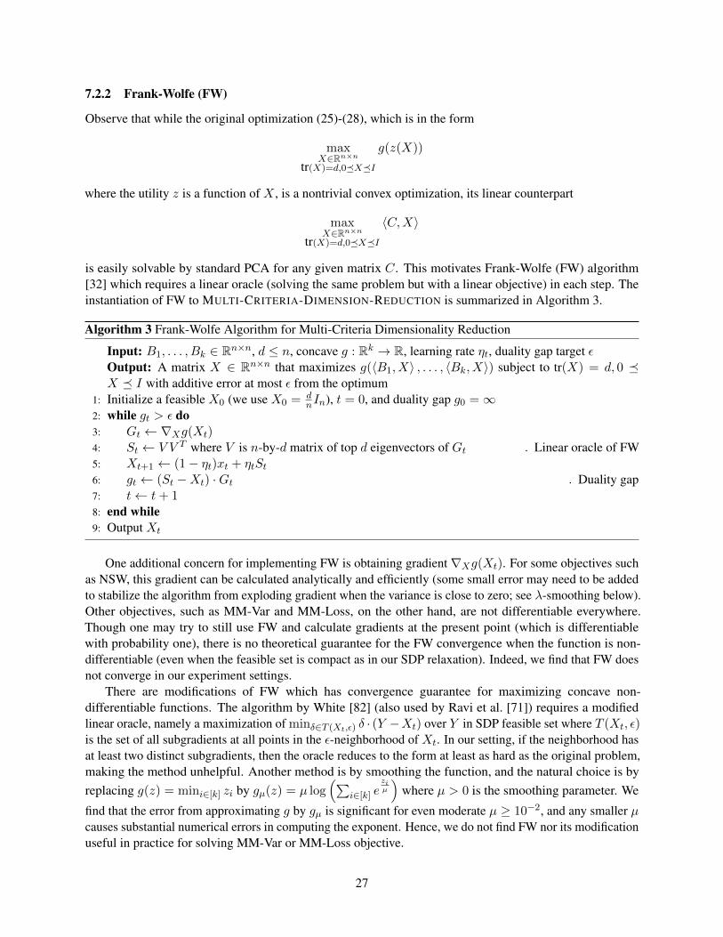
7.2.2 Frank-Wolfe (FW)

Observe that while the original optimization (25)-(28), which is in the form

maxX∈Rn×n

tr(X)=d,0XI

g(z(X))

where the utility z is a function of X , is a nontrivial convex optimization, its linear counterpart

maxX∈Rn×n

tr(X)=d,0XI

〈C,X〉

is easily solvable by standard PCA for any given matrix C. This motivates Frank-Wolfe (FW) algorithm[32] which requires a linear oracle (solving the same problem but with a linear objective) in each step. Theinstantiation of FW to MULTI-CRITERIA-DIMENSION-REDUCTION is summarized in Algorithm 3.

Algorithm 3 Frank-Wolfe Algorithm for Multi-Criteria Dimensionality Reduction

Input: B1, . . . , Bk ∈ Rn×n, d ≤ n, concave g : Rk → R, learning rate ηt, duality gap target εOutput: A matrix X ∈ Rn×n that maximizes g(〈B1, X〉 , . . . , 〈Bk, X〉) subject to tr(X) = d, 0 X I with additive error at most ε from the optimum

1: Initialize a feasible X0 (we use X0 = dnIn), t = 0, and duality gap g0 =∞

2: while gt > ε do3: Gt ← ∇Xg(Xt)4: St ← V V T where V is n-by-d matrix of top d eigenvectors of Gt . Linear oracle of FW5: Xt+1 ← (1− ηt)xt + ηtSt6: gt ← (St −Xt) ·Gt . Duality gap7: t← t+ 18: end while9: Output Xt

One additional concern for implementing FW is obtaining gradient ∇Xg(Xt). For some objectives suchas NSW, this gradient can be calculated analytically and efficiently (some small error may need to be addedto stabilize the algorithm from exploding gradient when the variance is close to zero; see λ-smoothing below).Other objectives, such as MM-Var and MM-Loss, on the other hand, are not differentiable everywhere.Though one may try to still use FW and calculate gradients at the present point (which is differentiablewith probability one), there is no theoretical guarantee for the FW convergence when the function is non-differentiable (even when the feasible set is compact as in our SDP relaxation). Indeed, we find that FW doesnot converge in our experiment settings.

There are modifications of FW which has convergence guarantee for maximizing concave non-differentiable functions. The algorithm by White [82] (also used by Ravi et al. [71]) requires a modifiedlinear oracle, namely a maximization of minδ∈T (Xt,ε) δ · (Y −Xt) over Y in SDP feasible set where T (Xt, ε)is the set of all subgradients at all points in the ε-neighborhood of Xt. In our setting, if the neighborhood hasat least two distinct subgradients, then the oracle reduces to the form at least as hard as the original problem,making the method unhelpful. Another method is by smoothing the function, and the natural choice is byreplacing g(z) = mini∈[k] zi by gµ(z) = µ log

(∑i∈[k] e

ziµ

)where µ > 0 is the smoothing parameter. We

find that the error from approximating g by gµ is significant for even moderate µ ≥ 10−2, and any smaller µcauses substantial numerical errors in computing the exponent. Hence, we do not find FW nor its modificationuseful in practice for solving MM-Var or MM-Loss objective.

27

Runtime analysis. The NSW objective can be ill-conditioned or even undefined when matrices Bi’s spanlow dimensions and those dimensions are distinct. This is due to log 〈Bi, X〉 not defined at 〈Bi, X〉 = 0 andhaving unbounded gradient when 〈Bi, X〉 is small. To stabilize the objective, we solve the λ-smoothed NSWobjective

maxX∈Rn×n

tr(X)=d,0XI

g(X) :=∑i∈[k]

log (〈Bi, X〉+ λ · ‖Bi‖F ) (33)

Here, λ > 0 is a regularizer, and the regularization term λ · ‖Bi‖F normalizes the effect of each group whentheir variances are small, regardless of their original sizes ‖Bi‖F . Since g(X) is now also Lipschitz, FW hasthe convergence guarantee as follows, which follows from the standard FW convergence bound [42]. Theproof can be found in Appendix A.4.

Theorem 7.2. Given n, k, d, λ and PSD B1, . . . , Bk ∈ Rn×n as an input to λ-smooth NSW (33), the t-thiterate Xt of Frank-Wolfe with step sizes ηs = 2/(s+ 1) satisfies

g∗ − g(Xt) ≤8kd

λ(t+ 2)(34)

where g∗ is the optimum of the optimization problem.

Theorem 7.2 implies that FW takes O(kdλε

)iterations to get an error bound ε for solving λ-smooth NSW.

Tuning in practice. In practice, we experiment with more aggressive learning rate schedule and line searchalgorithm. We found that FW converges quickly for NSW objective. However, FW does not converge forMM-Var and MM-Loss for any learning rate schedule, including the standard ηt = 1

t+2 and line search. Thisis consistent with, as we mentioned, that FW does not have convergence guarantee for non-differentiableobjectives.

7.2.3 Empirical runtime result on a large data set

We perform MW and FW heuristics on a large 1940 Colorado Census data set [5]. The data is preprocessedby one-hot encoding all discrete columns, ignoring columns with N/A, and normalizing the data to havemean zero and variance one on each feature. The preprocessed data set contains 661k data points and 7284columns. Data are partitioned into 16 groups based on 2 genders and 8 education levels. We solve the SDPrelaxation of MULTI-CRITERIA-DIMENSION-REDUCTION with MM-Var, MM-Loss, and NSW objectivesuntil achieving the duality gap of no more than 0.1% (in the case of NSW, the product of variances, not thesum of logarithmic of variances, is used to calculate this gap). The runtime results, in seconds, are in shownin Table 2. When n increases, the bottleneck of the experiment becomes the standard PCA itself. Sincespeeding up the standard PCA is not in the scope of this work, we capped the original dimension of data byselecting the first n dimensions out of 7284, so that the standard PCA can still be performed in a reasonableamount of time. We note that the rank violation of solutions are almost always zero, and are exactly onewhen it is not zero, similarly to what we found for Adult Income and Credit data sets [80, 83].

Runtime of MW. We found that MM-Var and MM-Loss objectives are solved efficiently by MW, whereasMW with gradient descent on the dual of NSW does not converge quickly. It is usual that the solution ofthe relaxation has rank exactly d, and in all those cases we are able to tune learning rates so that the lastiterate converges, giving a much faster convergence than the average iterate. For the Census data set, afterparameter tuning, MW runs 100-200 iterations on both objectives. MW for both Credit and Income data sets(n = 23, 59) on 4-6 groups on both objectives finishes in 10-20 iterations whenever the last iterate converges,giving a total runtime of less than few seconds. Each iteration of MW takes 1x-2x of an SVD algorithm.

28

Table 2: Runtime of MW and FW for solving MULTI-CRITERIA-DIMENSION-REDUCTION on differentfairness objectives and numbers of dimensions on the original 1940 Colorado Census data set. Runtimes ofthe standard PCA by SVD are included for comparison. All instances are solved to duality gap of at most0.1%. Times are in second(s).

Original Dimensions MM-Var (by MW) MM-Loss (by MW) NSW (by FW) Standard PCA (by SVD)n = 1000 77 65 11 0.22n = 2000 585 589 69 1.5

Therefore, the price of fairness in PCA for MW-Var and MM-Loss objectives is 200-400x runtime for largedata sets, and 20-40x runtime for medium data sets, as compared to the standard PCA without a fairnessconstraint.

Runtime of FW. FW converges quickly for NSW objective, and does not converge on MM-Var or MM-Loss. FW terminates in 10-20 iterations for Census Data. In practice, each iteration of FW has an overheadof 1.5x-3x of an SVD algorithm. We suspect codes can be optimized so that the constant overhead of eachiteration is closer to 1x, as the bottleneck in each iteration is one standard PCA. Therefore, the price offairness in PCA for NSW objective is 15-60x runtime compared to the standard PCA without a fairnessconstraint.

References

[1] Philip Adler, Casey Falk, Sorelle Friedler, Gabriel Rybeck, Carlos Scheidegger, Brandon Smith, andSuresh Venkatasubramanian. Auditing black-box models for indirect influence. In Proceedings of the16th International Conference on Data Mining, pages 1–10, 2016.

[2] Mahmoud Afifi and Abdelrahman Abdelhamed. Afif4: Deep gender classification based on adaboost-based fusion of isolated facial features and foggy faces. arXiv preprint arXiv:1706.04277, 2017.

[3] Wenbao Ai, Yongwei Huang, and Shuzhong Zhang. On the low rank solutions for linear matrixinequalities. Mathematics of Operations Research, 33(4):965–975, 2008.

[4] Julia Angwin, Jeff Larson, Surya Mattu, and Lauren Kirchner. Ma-chine bias - propublica. https://www.propublica.org/article/machine-bias-risk-assessments-in-criminal-sentencing, 2018.

[5] The U.S. National Archives and Records Administration. https://1940census.archives.gov/index.asp.Accessed on March 27th, 2020.

[6] Sanjeev Arora, Elad Hazan, and Satyen Kale. The multiplicative weights update method: a meta-algorithm and applications. Theory of Computing, 8(1):121–164, 2012.

[7] Afonso S Bandeira, Nicolas Boumal, and Vladislav Voroninski. On the low-rank approach for semidefi-nite programs arising in synchronization and community detection. In Conference on learning theory,pages 361–382, 2016.

[8] Alexander I Barvinok. Feasibility testing for systems of real quadratic equations. Discrete & Computa-tional Geometry, 10(1):1–13, 1993.

29

[9] Alexander I. Barvinok. Problems of distance geometry and convex properties of quadratic maps.Discrete & Computational Geometry, 13(2):189–202, 1995.

[10] Ahron Ben-Tal and Arkadi Nemirovski. Lectures on modern convex optimization: analysis, algorithms,and engineering applications, volume 2. Siam, 2001.

[11] Alex Beutel, Jilin Chen, Zhe Zhao, and Ed Huai-hsin Chi. Data decisions and theoretical implicationswhen adversarially learning fair representations. CoRR, abs/1707.00075, 2017.

[12] Amey Bhangale, Swastik Kopparty, and Sushant Sachdeva. Simultaneous approximation of constraintsatisfaction problems. In International Colloquium on Automata, Languages, and Programming, pages193–205. Springer, 2015.

[13] Amey Bhangale, Subhash Khot, Swastik Kopparty, Sushant Sachdeva, and Devanathan Thimvenkat-achari. Near-optimal approximation algorithm for simultaneous max-cut. In Proceedings of theTwenty-Ninth Annual ACM-SIAM Symposium on Discrete Algorithms, pages 1407–1425. Society forIndustrial and Applied Mathematics, 2018.

[14] F Bohnenblust. Joint positiveness of matrices. Unpublished manuscript, 48, 1948.

[15] Tolga Bolukbasi, Kai-Wei Chang, James Y Zou, Venkatesh Saligrama, and Adam T Kalai. Man is tocomputer programmer as woman is to homemaker? debiasing word embeddings. In Advances in neuralinformation processing systems, pages 4349–4357, 2016.

[16] Nicolas Boumal, Vlad Voroninski, and Afonso Bandeira. The non-convex burer-monteiro approachworks on smooth semidefinite programs. In Advances in Neural Information Processing Systems, pages2757–2765, 2016.

[17] Joy Buolamwini and Timnit Gebru. Gender shades: Intersectional accuracy disparities in commercialgender classification. In Conference on Fairness, Accountability and Transparency, pages 77–91, 2018.

[18] Samuel Burer and Renato DC Monteiro. A nonlinear programming algorithm for solving semidefiniteprograms via low-rank factorization. Mathematical Programming, 95(2):329–357, 2003.

[19] Samuel Burer and Renato DC Monteiro. Local minima and convergence in low-rank semidefiniteprogramming. Mathematical Programming, 103(3):427–444, 2005.

[20] Toon Calders and Sicco Verwer. Three naive Bayes approaches for discrimination-free classification.Data Mining and Knowledge Discovery, 21(2):277–292, 2010.

[21] Flavio Calmon, Dennis Wei, Bhanukiran Vinzamuri, Karthikeyan Natesan Ramamurthy, and Kush RVarshney. Optimized pre-processing for discrimination prevention. In Advances in Neural InformationProcessing Systems, pages 3992–4001, 2017.

[22] L Elisa Celis, Vijay Keswani, Damian Straszak, Amit Deshpande, Tarun Kathuria, and Nisheeth KVishnoi. Fair and diverse dpp-based data summarization. arXiv preprint arXiv:1802.04023, 2018.

[23] Flavio Chierichetti, Ravi Kumar, Silvio Lattanzi, and Sergei Vassilvitskii. Fair clustering throughfairlets. In Advances in Neural Information Processing Systems, pages 5029–5037, 2017.

[24] Alexandra Chouldechova. Fair prediction with disparate impact: A study of bias in recidivism predictioninstruments. Big data, 5(2):153–163, 2017.

30

[25] Kate Crawford. The trouble with bias, 2017. URL http://blog.revolutionanalytics.com/2017/12/the-trouble-with-bias-by-kate-crawford.html. Invited Talk byKate Crawford at NIPS 2017, Long Beach, CA.

[26] Kalyanmoy Deb. Multi-objective optimization. In Search methodologies, pages 403–449. Springer,2014.

[27] Cynthia Dwork, Moritz Hardt, Toniann Pitassi, Omer Reingold, and Richard Zemel. Fairness throughawareness. In Proceedings of the 3rd innovations in theoretical computer science conference, pages214–226. ACM, 2012.

[28] Danielle Ensign, Sorelle A. Friedler, Scott Neville, Carlos Eduardo Scheidegger, and Suresh Venkata-subramanian. Runaway feedback loops in predictive policing. Workshop on Fairness, Accountability,and Transparency in Machine Learning, 2017.

[29] Zuyuan Fang and Brahim Bensaou. Fair bandwidth sharing algorithms based on game theory frameworksfor wireless ad hoc networks. In IEEE infocom, volume 2, pages 1284–1295. Citeseer, 2004.

[30] Michael Feldman, Sorelle Friedler, John Moeller, Carlos Scheidegger, and Suresh Venkatasubramanian.Certifying and removing disparate impact. In Proceedings of the 21th ACM SIGKDD InternationalConference on Knowledge Discovery and Data Mining, pages 259–268, 2015.

[31] Benjamin Fish, Jeremy Kun, and Ádám Dániel Lelkes. A confidence-based approach for balancingfairness and accuracy. In Proceedings of the 16th SIAM International Conference on Data Mining,pages 144–152, 2016.

[32] Marguerite Frank and Philip Wolfe. An algorithm for quadratic programming. Naval research logisticsquarterly, 3(1-2):95–110, 1956.

[33] Timnit Gebru, Jamie Morgenstern, Briana Vecchione, Jennifer Wortman Vaughan, Hanna Wallach, HalDaumeé III, and Kate Crawford. Datasheets for datasets. arXiv preprint arXiv:1803.09010, 2018.

[34] Fabrizio Grandoni, R Ravi, Mohit Singh, and Rico Zenklusen. New approaches to multi-objectiveoptimization. Mathematical Programming, 146(1-2):525–554, 2014.

[35] D Yu Grigor’ev and NN Vorobjov Jr. Solving systems of polynomial inequalities in subexponentialtime. Journal of Symbolic Computation, 5(1-2):37–64, 1988.

[36] Dima Grigoriev and Dmitrii V Pasechnik. Polynomial-time computing over quadratic maps i: samplingin real algebraic sets. Computational complexity, 14(1):20–52, 2005.

[37] Sara Hajian and Josep Domingo-Ferrer. A methodology for direct and indirect discrimination preventionin data mining. IEEE Transactions on Knowledge and Data Engineering, 25(7):1445–1459, 2013.

[38] Moritz Hardt, Eric Price, Nati Srebro, et al. Equality of opportunity in supervised learning. In Advancesin neural information processing systems, pages 3315–3323, 2016.

[39] Harold Hotelling. Analysis of a complex of statistical variables into principal components. Journal ofeducational psychology, 24(6):417, 1933.

[40] Gary B. Huang, Manu Ramesh, Tamara Berg, and Erik Learned-Miller. Labeled faces in the wild:A database for studying face recognition in unconstrained environments. Technical Report 07-49,University of Massachusetts, Amherst, October 2007.

31

[41] Amy F Iezzoni and Marvin P Pritts. Applications of principal component analysis to horticulturalresearch. HortScience, 26(4):334–338, 1991.

[42] Martin Jaggi. Revisiting frank-wolfe: Projection-free sparse convex optimization. In Proceedings of the30th international conference on machine learning, number CONF, pages 427–435, 2013.

[43] Ian T Jolliffe. Principal component analysis and factor analysis. In Principal component analysis, pages115–128. Springer, 1986.

[44] Matthew Joseph, Michael Kearns, Jamie H Morgenstern, and Aaron Roth. Fairness in learning: Classicand contextual bandits. In Advances in Neural Information Processing Systems, pages 325–333, 2016.

[45] Ehud Kalai. Proportional solutions to bargaining situations: interpersonal utility comparisons. Econo-metrica: Journal of the Econometric Society, pages 1623–1630, 1977.

[46] Ehud Kalai, Meir Smorodinsky, et al. Other solutions to nash bargaining problem. Econometrica, 43(3):513–518, 1975.

[47] Faisal Kamiran and Toon Calders. Data preprocessing techniques for classification without discrimina-tion. Knowledge and Information Systems, 33(1):1–33, 2011.

[48] Faisal Kamiran, Toon Calders, and Mykola Pechenizkiy. Discrimination aware decision tree learning.In Proceedings of the 10th IEEE International Conference on Data Mining, pages 869–874, 2010.

[49] Faisal Kamiran, Asim Karim, and Xiangliang Zhang. Decision theory for discrimination-awareclassification. In Proceedings of the 12th IEEE International Conference on Data Mining, pages924–929, 2012.

[50] Toshihiro Kamishima, Shotaro Akaho, Hideki Asoh, and Jun Sakuma. Fairness-aware classifier withprejudice remover regularizer. In Proceedings of the European Conference on Machine Learning andKnowledge Discovery in Databases, pages 35–50, 2012.

[51] Mamoru Kaneko and Kenjiro Nakamura. The nash social welfare function. Econometrica: Journal ofthe Econometric Society, pages 423–435, 1979.

[52] Sampath Kannan, Michael Kearns, Jamie Morgenstern, Mallesh M. Pai, Aaron Roth, Rakesh V. Vohra,and Zhiwei Steven Wu. Fairness incentives for myopic agents. In Proceedings of the 2017 ACMConference on Economics and Computation, pages 369–386, 2017.

[53] Matthew Kay, Cynthia Matuszek, and Sean A Munson. Unequal representation and gender stereotypesin image search results for occupations. In Proceedings of the 33rd Annual ACM Conference on HumanFactors in Computing Systems, pages 3819–3828. ACM, 2015.

[54] Jon Kleinberg, Sendhil Mullainathan, and Manish Raghavan. Inherent trade-offs in the fair determinationof risk scores. arXiv preprint arXiv:1609.05807, 2016.

[55] Matthäus Kleindessner, Pranjal Awasthi, and Jamie Morgenstern. Fair k-center clustering for datasummarization. In Proceedings of the 36th International Conference on Machine Learning, 2019.

[56] Matthäus Kleindessner, Samira Samadi, Pranjal Awasthi, and Jamie Morgenstern. Guarantees forspectral clustering with fairness constraints. In Proceedings of the 36th International Conference onMachine Learning, 2019.

32

[57] Joseph B Kruskal. Multidimensional scaling by optimizing goodness of fit to a nonmetric hypothesis.Psychometrika, 29(1):1–27, 1964.

[58] Lap Chi Lau, Ramamoorthi Ravi, and Mohit Singh. Iterative methods in combinatorial optimization,volume 46. Cambridge University Press, 2011.

[59] Zachary Lipton, Julian McAuley, and Alexandra Chouldechova. Does mitigating ml’s impact disparityrequire treatment disparity? In Advances in Neural Information Processing Systems, pages 8125–8135,2018.

[60] Binh Thanh Luong, Salvatore Ruggieri, and Franco Turini. k-NN as an implementation of situation test-ing for discrimination discovery and prevention. In Proceedings of the 17th ACM SIGKDD internationalconference on Knowledge discovery and data mining, pages 502–510. ACM, 2011.

[61] Laurens van der Maaten and Geoffrey Hinton. Visualizing data using t-sne. Journal of machine learningresearch, 9(Nov):2579–2605, 2008.

[62] David Madras, Elliot Creager, Toniann Pitassi, and Richard Zemel. Learning adversarially fair andtransferable representations. In Proceedings of the 35th International Conference on Machine Learning,pages 3384–3393, 2018.

[63] John F Nash Jr. The bargaining problem. Econometrica: Journal of the Econometric Society, pages155–162, 1950.

[64] Arkadiı Semenovich Nemirovsky and David Borisovich Yudin. Problem complexity and methodefficiency in optimization. 1983.

[65] Safiya Umoja Noble. Algorithms of oppression: How search engines reinforce racism. nyu Press, 2018.

[66] Matt Olfat and Anil Aswani. Convex formulations for fair principal component analysis. arXiv preprintarXiv:1802.03765, 2018.

[67] Gábor Pataki. On the rank of extreme matrices in semi-definite programs and the multiplicity of optimaleigenvalues. Mathematics of operations research, 23(2):339–358, 1998.

[68] Karl Pearson. On lines and planes of closest fit to systems of points in space. The London, Edinburgh,and Dublin Philosophical Magazine and Journal of Science, 2(11):559–572, 1901.

[69] Dino Pedreshi, Salvatore Ruggieri, and Franco Turini. Discrimination-aware data mining. In Proceed-ings of the 14th ACM SIGKDD international conference on Knowledge discovery and data mining,pages 560–568. ACM, 2008.

[70] Ram Ravi and Michel X Goemans. The constrained minimum spanning tree problem. In ScandinavianWorkshop on Algorithm Theory, pages 66–75. Springer, 1996.

[71] Sathya N Ravi, Maxwell D Collins, and Vikas Singh. A deterministic nonsmooth frank wolfe algorithmwith coreset guarantees. Informs Journal on Optimization, 1(2):120–142, 2019.

[72] Soumya Raychaudhuri, Joshua M Stuart, and Russ B Altman. Principal components analysis tosummarize microarray experiments: application to sporulation time series. In Biocomputing 2000,pages 455–466. World Scientific, 1999.

[73] Sam T Roweis and Lawrence K Saul. Nonlinear dimensionality reduction by locally linear embedding.science, 290(5500):2323–2326, 2000.

33

[74] Samira Samadi, Uthaipon Tantipongpipat, Jamie H Morgenstern, Mohit Singh, and Santosh Vempala.The price of fair pca: One extra dimension. In Advances in Neural Information Processing Systems,pages 10976–10987, 2018.

[75] Tom Simonite. When it comes to gorillas, google photos remains blind. https://www.wired.com/story/when-it-comes-to-gorillas-google-photos-remains-blind/, Jan2018.

[76] Anthony Man-Cho So, Yinyu Ye, and Jiawei Zhang. A unified theorem on sdp rank reduction.Mathematics of Operations Research, 33(4):910–920, 2008.

[77] Latanya Sweeney. Discrimination in online ad delivery. Communications of the ACM, 56(5):44–54,2013.

[78] Joshua B Tenenbaum, Vin De Silva, and John C Langford. A global geometric framework for nonlineardimensionality reduction. science, 290(5500):2319–2323, 2000.

[79] Twitter. Jacky lives: Google photos, y’all fucked up. My friend’s not a gorilla. https://twitter.com/jackyalcine/status/615329515909156865, June 2015.

[80] UC Irvine Repository. Adult data set. Machine Learning Repository, Center for Machine Learning andIntelligent Systems. https://archive.ics.uci.edu/ml/datasets/adult. Accessed May 2019.

[81] Guiyi Wei, Athanasios V Vasilakos, Yao Zheng, and Naixue Xiong. A game-theoretic method of fairresource allocation for cloud computing services. The journal of supercomputing, 54(2):252–269, 2010.

[82] DJ White. Extension of the frank-wolfe algorithm to concave nondifferentiable objective functions.Journal of optimization theory and applications, 78(2):283–301, 1993.

[83] I-Cheng Yeh and Che-hui Lien. The comparisons of data mining techniques for the predictive accuracyof probability of default of credit card clients. Expert Systems with Applications, 36(2):2473–2480,2009.

[84] Muhammad Zafar, Isabel Valera, Manuel Gomez-Rodriguez, and Krishna Gummadi. Fairness con-straints: A mechanism for fair classification. CoRR, abs/1507.05259, 2015.

[85] Rich Zemel, Yu Wu, Kevin Swersky, Toni Pitassi, and Cynthia Dwork. Learning fair representations. InInternational Conference on Machine Learning, pages 325–333, 2013.

[86] Brian Hu Zhang, Blake Lemoine, and Margaret Mitchell. Mitigating unwanted biases with adversariallearning. arXiv preprint arXiv:1801.07593, 2018.

34

A Proofs

A.1 Proof of Theorem 3.1 by local optimality

Before proving Theorem 3.1, we first state some notations and lemmas. We denote by A1 ∈ Rm1×n, A2 ∈Rm2×n data matrices of two groups, with rows as data points, in n dimensions that are to be projected onto ddimensions. Let Sd denote the set of all d-dimensional subspaces of Rn. For U ∈ Sd, we let PU ∈ Pd be amatrix which has an orthonormal basis of the subspace U as its columns.

For each matrix M , we let P ∗M ∈ arg maxQ∈Pd ‖MQ‖2F . We denote loss(M,U) = ‖MP ∗M‖2F −‖MPU‖2F be the loss of data M by a projection onto U . For data matrix A in n dimensions, we letgA(U) = ‖APU‖2F for U ∈ Sd. We let h(U) be the marginal loss objective (16) given by a projection matrixPU to be minimized. We note that gA, h, and loss are well-defined since their values do not change based onthe orthonormal basis representation of U .

For a function f : Pd → R, we call P ∗ ∈ Pd a local maximum of f if there exists ε > 0 suchthat f(P ∗) ≥ f(P ) for all P ∈ Pd with ‖P − P ∗‖F < ε (we note that any P ∈ Pd always has an ε-neighbor by a slight change in one column while remaining in the orthogonal complement of the rest forall d < n). We define an ε-neighborhood of U ∈ Sd as the set of all d-dimensional subspaces V ∈ Sdsuch that there exist orthonormal bases PU , PV of U, V with ‖PU − PV ‖F < ε. (More generally, welet d(U, V ) := inf ‖PU − PV ‖F : PU , PV are orthonormal bases of U, V be the metric on Sd.) We thendefine the local optimality and continuity of gA, h, and loss accordingly.

We state the a property of gA which is a building block for the proof of Theorem 3.1.

Lemma A.1. Given a matrix A ∈ Ra×n, the value of the function gA at any local maximum is the same.

Before we prove this lemma, we prove use it to prove Theorem 3.1.

Proof of Theorem 3.1: We prove by a contradiction. Let W be a global minimum of h and assume that

loss(A1,W ) > loss(A2,W ). (35)

Since loss is continuous, there exists ε > 0 such that for any Wε in the ε-neighborhood of W , h(Wε) =loss(A1,W ). Since W is a global minimum of h, it is a local minimum of loss(A1,W ), or equivalently alocal maximum of gA1 .

Let v1, . . . , vn be an orthonormal basis of the eigenvectors of AT1 A1 corresponding to eigenvaluesλ1 ≥ λ2 ≥ . . . ≥ λn. Let V ∗ be the subspace spanned by v1, . . . , vd. Note that loss(A1, V

∗) = 0. Sincethe loss is always non-negative for both A1 and A2, (35) implies that loss(A1,W ) > 0. Therefore, W 6= V ∗

and gA1(V ∗) > gA1(W ). By Lemma A.1, this is in contradiction with V ∗ being a global maximum and Wbeing a local maximum of gA1 . 2

We now prove Lemma A.1. We will also use the following formula: given a matrix V = [v1, . . . , vd] ∈Rn×d with orthonormal columns and U = span(V ), we have

gA(U) = ‖AV ‖2F =d∑i=1

‖Avi‖2 (36)

Formula (36) is straightforward from the definitions of gA and Frobenius norm.

Proof of Lemma A.1: We prove that the value of function gA at its local maxima is equal to its value at itsglobal maximum, which we know is the subspace spanned by a top d eigenvectors of ATA. Let v1, . . . , vnbe an orthonormal basis of eigenvectors of ATA with corresponding eigenvalues λ1 ≥ . . . ≥ λn where tiesare broken arbitrarily. Let V ∗ be the subspace spanned by v1, . . . , vd and let U ∈ Sd be a local optimum

35

of gA. We assume for contradiction that gA(U) < gA(V ∗). We will show that there exists a small constantC > 0 such that for all ε ∈ (0, C), there exists Uε in the ε-neighborhood of U which strictly increases gA.This will contradict the local optimality of U .

As gA(U) < gA(V ∗), we have U 6= V ∗. Let k be the smallest index such that vk /∈ U . Extendv1, . . . , vk−1 to an orthonormal basis of U : v1, . . . , vk−1, v

′k, . . . , v

′d. Let q ≥ k be the smallest index

such that ‖Avq‖2 > ‖Av′q‖2 (such an index q must exist because gA(U) < gA(V ∗)). Without loss ofgenerality, we can assume that q = 1. Therefore, we assume that v1, the top eigenvector of ATA, is not in Uand that v1 strictly maximizes the function ‖Au‖2 over the space of unit vectors u. Specifically, for any unitvector u ∈ U , ‖Au‖2 < ‖Av1‖2 = λ1. We distinguish two cases:

Case v1 ⊥ U . Let wε =√

1− ε2u1 + εv1. Then we have ‖wε‖ = 1 and that wε, u2, . . . , ud is anorthonormal set of vectors. We set Uε = spanwε, u2, . . . , ud and claim that gA(Uε)−gA(U) > 0 for all ε ∈(0, 1). By (36), gA(Uε) = ‖Awε‖2+‖Au2‖2+. . .+‖Aud‖2 and gA(U) = ‖Au1‖2+‖Au2‖2+. . .+‖Aud‖2.Hence, gA(Uε)− gA(U) = ‖Awε‖2 − ‖Au1‖2. We have

‖Awε‖2 − ‖Au1‖2 = ‖A(√

1− ε2u1 + εv1)‖2 − ‖Au1‖2

= (√

1− ε2uT1 + εvT1 )ATA(√

1− ε2u1 + εv1)− ‖Au1‖2

= (1− ε2)uT1 ATAu1 + ε2vT1 A

TAv1 + 2√

1− ε2εuT1 ATAv1 − ‖Au1‖2

= (1− ε2)‖Au1‖2 + ε2λ1 + 2ε√

1− ε2uT1 ATAv1 − ‖Au1‖2

= ε2(λ1 − ‖Au1‖2) + 2ε√

1− ε2uT1 ATAv1

Next, we have uT1 ATAv1 = uT1 (λ1v1) = λ1u

T1 v1 = 0 since v1 is an eigenvector of ATA and v1 ⊥ u1. This

and the fact that ‖Au1‖2 < λ1 give

‖Awε‖2 − ‖Au1‖2 = ε2(λ1 − ‖Au1‖2) > 0

as desired.

Case v1 6⊥ U . Let v1 =√

1− a2z1 + az2 where z1 ∈ U , z2 ⊥ U , a ∈ (0, 1) and‖z1‖ = ‖z2‖ = 1, so theprojection of v1 to U is

√1− a2z1. Note that z2 6= 0 and a > 0 since v1 /∈ U , and that a < 1 since v1 6⊥ U .

We extend z1 to an orthonormal basis of U : z1, u2, . . . , uk.Consider the unit vector wε =

√1− ε2z1 + εz2 for ε ∈ (0, 1). Let Uε := spanwε, u2, . . . , ud. Note

that wε, u2, . . . , ud is orthonormal for any ε since both z1 and z2 are orthogonal to all of u2, . . . , ud andwε is in the span of z1, z2. Since the chosen orthonormal bases of Uε and U differ only in wε and z1, by (36),gA(Uε)− gA(U) = ‖Awε‖2 − ‖Az1‖2. We can write

wε =

(√1− ε2 − ε

√1− a2

a

)z1 +

ε

a

(√1− a2z1 + az2

)=

(√1− ε2 − ε

√1− a2

a

)z1 +

ε

av1.

36

Thus, by ATAv1 = λ1v1 (as v1 is an eigenvector with eigenvalue λ1) and zT1 v1 =√

1− a2, we have

‖Awε‖2 =

(√1− ε2 − ε

√1− a2

a

)2

‖Az1‖2 +ε2

a2‖Av1‖2 + 2

ε

a

(√1− ε2 − ε

√1− a2

a

)zT1 A

TAv1

=

(1− ε2 +

ε2(1− a2)

a2− 2

ε√

(1− ε2)(1− a2)

a

)‖Az1‖2 +

ε2

a2λ1

+ 2ε

a

(√1− ε2 − ε

√1− a2

a

)λ1z

T1 v1

=

(1− 2ε2 +

ε2

a2− 2

ε√

(1− ε2)(1− a2)

a

)‖Az1‖2

+

(ε2

a2+ 2

ε√

(1− ε2)(1− a2)

a− 2

ε2(1− a2)

a2

)λ1

= ‖Az1‖2 + (λ1 − ‖Az1‖2)

(2ε√

(1− ε2)(1− a2)

a+ 2ε2 − ε2

a2

)> ‖Az1‖2.

The last inequality follows since λ1 > ‖Az1‖2. Now, we let 0 < ε < 11+b for b = 4a2(1 − a2) so that

2ε√

(1−ε2)(1−a2)

a > ε2

a2. Then, ‖Awε‖2 > ‖Az1‖2 and therefore gA(Uε) > gA(U) for all such ε. 2

A.2 Proof of Theorem 3.1 by SDP relaxation

We remark that Theorem 3.1 also follows from using SDP relaxation formulation of MULTI-CRITERIA-DIMENSION-REDUCTION for marginal loss objective, which is

minX∈Rn×n

z subject to (37)

βi − 〈ATi Ai, X〉 ≤ z , i ∈ 1, 2 (38)

tr(X) ≤ d (39)

0 X I (40)

where βi = maxQ∈Pd ‖AiQ‖2. We provide a proof here as another application of the relaxation.

Proof of Theorem 3.1: Let X∗ be an extreme solution of the SDP (37)-(40). Suppose the marginal loss oftwo groups are not equal; without loss of generality, we have

β1 − 〈AT1 A1, X〉 > β2 − 〈AT2 A2, X〉.

Since the constraint β2 − 〈AT2 A2, X〉 ≤ z is not tight, we can delete it and the new SDP does not change theoptimal solution. However, an optimal solution of the new SDP, which now has only one group, is a standardPCA solution of the first group. This solution gives a loss of zero, so the optimum of the new SDP is zero.Therefore, the optimum of original SDP (37)-(40) is also zero. However, since the losses of both groups arealways non-negative, they must be zero and hence are equal. 2

37

A.3 Proof of MW convergence

Here we prove Theorem 7.1 using the mirror descent convergence [64]. When mirror descent is performedover a simplex, and the convergence guarantee from mirror descent is simplified as follows. We write∆k :=

w ∈ Rk : w ≥ 0,

∑i∈[k]wi = 1

.

Theorem A.2. ([64]) Consider a problem of maximizing a concave function h(w) over w ∈ ∆k whereh(u) − h(v) ≤ L ‖u− v‖1 for u, v ∈ ∆k. The t-th iterate w(t) of the mirror descent algorithm withnegative entropy potential function R(w) =

∑ki=1wi logwi, step size η, and the initial solution w(0) =

(1/k, . . . , 1/k) satisfies

h∗ − h(w(t)) ≤ log k

ηt+η

2L2 (41)

where h∗ is the optimum of the maximization problem.

We apply Theorem A.2 to obtain the convergence bound for MULTI-CRITERIA-DIMENSION-REDUCTION for fairness criteria in the "max-min" type including MM-Var and MM-Loss.

Proof of Theorem 7.1. We showed earlier that the dual problem of maximizing g is

infw∈∆k

(h(w) := max

X∈Ω

k∑i=1

wi 〈Bi, X〉

)

and that MW algorithm is equivalent to mirror descent on h(w) over w ∈ ∆k. Applying Theorem A.2 and

substituting η =√

log k2T L, the desired convergence bound follows, so it remains to show that h(u)− h(v) ≤

L ‖u− v‖1 for u, v ∈ ∆k. Let X∗u ∈ arg maxX∈Ω

∑ki=1 ui 〈Bi, X〉. We have

h(u) =k∑i=1

ui 〈Bi, X∗u〉 =k∑i=1

vi 〈Bi, X∗u〉+k∑i=1

(ui − vi) · 〈Bi, X∗u〉

≤ h(v) +k∑i=1

|ui − vi| · 〈Bi, X∗u〉

≤ h(v) +

k∑i=1

|ui − vi| · tr(Bi) ≤ h(v) + ‖u− v‖1 · L

where the first inequality follows from Bi, X∗u 0 so that their inner product is non-negative, and the second

follows from Bi 0 and X∗u I . This finishes the proof.

A.4 Proof of NSW convergence

We have a standard convergence of FW for differentiable and L-Lipschitz objective functions as follows.

Theorem A.3. ([42]) Consider a maximization problem of an L-Lipschitz concave function g(X) over aconvex feasible set D of diameter diam(D) := maxX,Y ∈D ‖X − Y ‖2. The t-th iterate Xt of Frank-Wolfewith step sizes ηs = 2/(s+ 1) satisfies

g∗ − g(Xt) ≤2L · diam2(D)

t+ 2(42)

where g∗ is the optimum of the maximization problem.

38

The theorem gives the proof of Theorem 7.2 as follow(s).

Proof of Theorem 7.2. We first show that g is L-Lipschitz for L = kλ . We have

‖∇Xg(X)‖F =

∥∥∥∥∥∥∑i∈[k]

Bi〈Bi, X〉+ λ · ‖Bi‖F

∥∥∥∥∥∥ ≤∑i∈[k]

‖Bi‖Fλ · ‖Bi‖F

=k

λ

as claimed. We write Ω = X ∈ Rn×n : tr(X) = d, 0 X I. By the convergence of FW in TheoremA.3, it remains to show that diam(Ω) ≤ 2

√d. For any X ∈ Ω, let σi(X) be the eigenvalues of X in the

descending order. Then, we have ‖X‖2F =∑

i∈[n] σ2i (X),

∑i∈[n] σi(X) ≤ d, and σi(X) ∈ [0, 1] for all

i by the constraints in Ω. Since a function h(x) = x2 is convex,∑

i∈[n] σ2i (X) is maximized subject to∑

i∈[n] σi(X) = 1 when σ1(X) = . . . = σd(X) = 1 and σd+1(X) = . . . = σn(X) = 0. So, we have‖X‖2F ≤ d, and therefore

maxX,Y ∈Ω

‖X − Y ‖F ≤ maxX∈Ω‖X‖F + max

Y ∈Ω‖Y ‖F ≤ 2

√d (43)

as needed.

B Tightness of the rank violation bound

Here, we show that the bound of rank of extreme solutions in Theorem 1.8 is tight by the following statement.

Lemma B.1. For any n, d, and s such that d ≤ n and 1 ≤ s ≤ n− d, there exist m = (s+1)(s+2)2 − 1 real

matrices A1, . . . , Am and a real matrix C, all of dimension n× n, and b1, . . . bm ∈ R such that SDP(I) isfeasible and all of its solutions have rank at least d+ s.

The example of instance is modified from [14] (and can also be found in [3]) to match our SDP that hasthe additional X I constraint.

Proof. We construct the constraints of SDP(I) so that the feasible set isX =

[λIs+1 X12

X21 X22

]∈ Rn×n : λ ∈ R, tr(X) ≤ d, 0 X In

(44)

This can be done by m constraint of the form (6) (e.g. by using s(s+1)2 equality constraints to set off-diagonal

entries of top (s + 1) × (s + 1) submatrix to zero, and the rest to set diagonal entries to be identical). Tofinish the construction of the instance, we set

C = diag(0, . . . , 0︸ ︷︷ ︸s times

, 1, . . . , 1︸ ︷︷ ︸d times

, 0, . . . , 0︸ ︷︷ ︸n−s−d times

)

Then, we claim that SDP(I) has an extreme solution

X∗ = diag(1/s, . . . , 1/s︸ ︷︷ ︸s+1 times

, 1, . . . , 1︸ ︷︷ ︸d−1 times

, 0, . . . , 0︸ ︷︷ ︸n−s−d times

) (45)

We first show that X∗ is an optimal solution. Let x1, . . . , xn be diagonal entries of X in the feasible set. By0 X I , we have xi = ei

TXei ∈ [0, 1] where ei is the unit vector at coordinate i. This fact, combinedwith tr(X) =

∑ni=1 xi ≤ d, shows that 〈C,X〉 is maximized when diag(X) is as described in (45).

39

We now show that X∗ is extreme. In fact, we show that X∗ is the unique solution and hence necessarilyextreme (since the feasible set is convex and compact). From the argument above, any solution X =[xij ]i,j∈[n] must satisfy diag(X) = diag(X∗), and it remains to show that off-diagonal entries must be zero.Because every 2 × 2 principle minor of X is non-negative, we have xij = 0 if i ∈ s+ d+ 1, . . . , n orj ∈ s+ d+ 1, . . . , n. We know that xij = 0 for all i, j ≤ s+ 1 such that i 6= j by the constraints in (44),so it remains to show that xij = 0 for s+ 2 ≤ i ≤ d+ s and j ≤ d+ s such that i 6= j.

Let i, j be one of such pair. We claim that the bigger eigenvalue of the 2× 2 submatrix[xii xijxij xjj

]is at

least max xii, xjj, with a strict equality if and only if xij 6= 0. Let p(t) be the characteristic polynomialof the matrix. Observe that p(xii), p(xjj) ≤ 0 (< 0 if xij 6= 0 and = 0 if xij = 0) and that p(t′) > 0 for asufficiently large t′ > max xii, xjj. Hence, there must be a root of p(t) in between max xii, xjj and t′,and the claim follows. Now, for the pair i, j, we have xjj = 1. By Cauchy’s Interlacing Theorem, X Iimplies that any 2 × 2 submatrix of X has both eigvenvalues at most 1. Therefore, the claim implies thatxij = 0.

40