April 18, 2023 Slide 1

Multicollinarity: Definition• Multicollinarity originally it meant the existence of a “perfect,” or

exact, linear relationship among some or all explanatory variables of a regression model.

• Multicollinarity is the condition where the independent variables are related to each other. Causation is not implied by Multicollinarity.

• As any two (or more) variables become more and more closely correlated, the condition worsens, and ‘approaches singularity’.

• Since the X's are supposed to be fixed, this a sample problem.

• Since Multicollinarity is almost always present, it is a problem of degree, not merely existence.

Example • As a numerical example, consider the following hypothetical data:• X2 X3 X*3• 10 50 52• 15 75 75• 18 90 97• 24 120 129• 30 150 152

• It is apparent that X3i = 5X2i . Therefore, there is perfect colinearity between X2 and X3 since the coefficient of correlation r23 is unity. The variable X*3 was created from X3 by simply adding to it the following numbers, which were taken from a table of random numbers: 2, 0, 7, 9, 2. Now there is no longer perfect collinearity between X2 and X*3. (X3i = 5X2i + vi ) However, the two variables are highly correlated because calculations will show that the coefficient of correlation between them is 0.9959.

Diagrammatic Presentation

• The preceding algebraic approach to Multicollinarity can be portrayed in Figure 10.1). In this figure the circles Y, X2, and X3 represent, respectively, the variations in Y (the dependent variable) and X2 and X3 (the explanatory variables). The degree of collinearity can be measured by the extent of the overlap (shaded area) of the X2 and X3 circles. In the extreme, if X2 and X3 were to overlap completely (or if X2 were completely inside X3, or vice versa), collinearity would be perfect.

Degree of Multicollinarity

April 18, 2023 Slide 5

Multicollinarity: Implications• Why does the classical linear regression model assume

that there is no Multicollinarity among the X’s? The reasoning is this:

• If Multicollinarity is perfect, the regression coefficients of the X variables are indeterminate and their standard errors are infinite.

• If Multicollinarity is less than perfect, the regression coefficients, although determinate, possess large standard errors which means the coefficients cannot be estimated with great precision or accuracy.

Multicollinarity: Causes

• 1. The data collection method employed, for example, sampling over a limited range of the values taken by the regressors in the population.

• 2. Constraints on the model or in the population being sampled. For example, in the regression of electricity consumption on income (X2) and house size (X3) (High X2 always mean high X3).

• 3. Model specification, for example, adding polynomial terms to a regression model, especially when the range of the X variable is small.

• 4. An over determined model. This happens when the model has more explanatory variables than the number of observations.

An additional reason for Multicollinarity, especially in time series data, may be that the regressors included in the model share a common trend, that is, they all increase or decrease over time.

PRACTICAL CONSEQUENCES OF MULTICOLLINEARITY

• In cases of near or high Multicollinarity, one is likely to encounter the following consequences:

• 1. Although BLUE, the OLS estimators have large variances and covariance's, making precise estimation difficult.

• 2. Because of consequence 1, the confidence intervals tend to be much wider, leading to the acceptance of the “zero null hypothesis” (i.e., the true population coefficient is zero) more readily.

• 3. Also because of consequence 1, the t ratio of one or more coefficients tends to be statistically insignificant.

• 4. Although the t ratio of one or more coefficients is statistically insignificant, R2 can be very high.

• 5. The OLS estimators and their standard errors can be sensitive to small changes in the data. The preceding consequences can be demonstrated as follows.

Example

Explanation

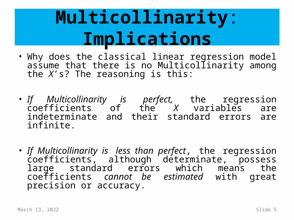
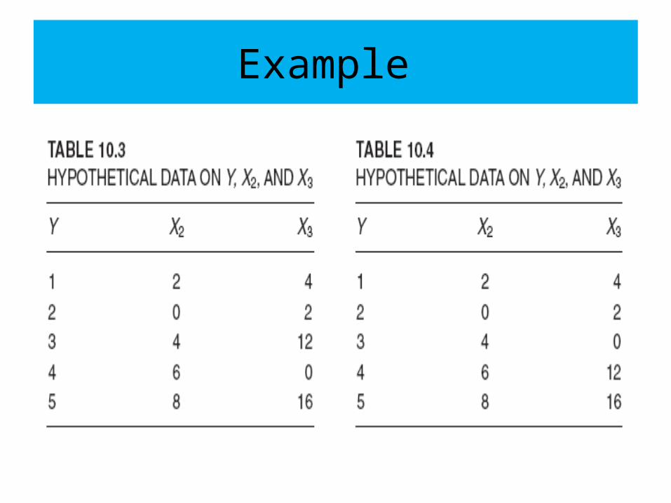
• As long as multicollinearity is not perfect, estimation of the regression coefficients is possible but the estimates and their standard errors become very sensitive to even the slightest change in the data.

• To see this, consider Table 10.3. Based on these data, we obtain the following multiple regression:Yˆi = 1.1939 + 0.4463X2i + 0.0030X3i (0.7737) (0.1848) (0.0851)

t = (1.5431) (2.4151) (0.0358) (10.5.6)

R2 = 0.8101 • cov (βˆ2, βˆ3) = −0.00868

Explanation• Regression (10.5.6) shows that none of the regression coefficients is

individually significant at the conventional 1 or 5 percent levels of significance, although βˆ2 is significant at the 10 percent level on the basis of a one-tail t test.

• Using the data of Table 10.4, we now obtain:Yˆi = 1.2108 + 0.4014X2i + 0.0270X3i

(0.7480) (0.2721) (0.1252)t = (1.6187) (1.4752) (0.2158) (10.5.7)R2 = 0.8143 cov (βˆ2, βˆ3) = −0.0282

• As a result of a slight change in the data, we see that βˆ2, which was statistically significant before at the 10 percent level of significance, is no longer significant. Also note that in (10.5.6) cov (βˆ2, βˆ3) = −0.00868 whereas in (10.5.7) it is −0.0282, a more than threefold increase. All these changes may be attributable to increased Multicollinarity: In (10.5.6) r23 = 0.5523, whereas in (10.5.7) it is 0.8285. Similarly, the standard errors of βˆ2 and βˆ3 increase between the two regressions, a usual symptom of collinearity.

Example

AN ILLUSTRATIVE EXAMPLE: CONSUMPTION EXPENDITUREIN RELATION TO INCOME AND WEALTH

• Let us reconsider the consumption–income example in table 10.5. we obtain the following regression:

Yˆi = 24.7747 + 0.9415X2i − 0.0424X3i (6.7525) (0.8229) (0.0807)

t = (3.6690) (1.1442) (−0.5261)

R2 = 0.9635 R¯2 = 0.9531 • Regression (10.6.1) shows that income and wealth

together explain about 96 percent of the variation in consumption expenditure, and yet neither of the slope coefficients is individually statistically significant. The wealth variable has the wrong sign. Although βˆ2 and βˆ3 are individually statistically insignificant, if we test the hypothesis that β2 = β3 = 0 simultaneously, this hypothesis can be rejected, as Table 10.6 shows.

Illustration

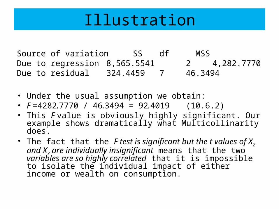
Source of variation SS df MSSDue to regression 8,565.5541 2 4,282.7770Due to residual 324.4459 7 46.3494

• Under the usual assumption we obtain:• F =4282.7770 / 46.3494 = 92.4019

(10.6.2)• This F value is obviously highly significant. Our example shows

dramatically what Multicollinarity does. • The fact that the F test is significant but the t values of X2 and X3 are

individually insignificant means that the two variables are so highly correlated that it is impossible to isolate the individual impact of either income or wealth on consumption.

Detection of Multicollinarity

• 1. High R2 but few significant t ratios. If R2 is high, say, in excess of 0.8, the F test in most cases will reject the hypothesis that the partial slope coefficients are simultaneously equal to zero, but the individual t tests will show that none or very few of the partial slope coefficients are statistically different from zero.

Detection of Multicollinarity• 2. Examination of partial correlations. Because of the

problem just mentioned in relying on zero-order correlations, Farrar and Glauber have suggested that one should look at the partial correlation coefficients. Thus, in the regression of Y on X2, X3, and X4, a finding that R2

1.234 is very high but r2

12.34, r213.24, and r2

14.23 are comparatively low may suggest that the variables X2, X3, and X4 are highly intercorrelated and that at least one of these variables is superfluous.

• Although a study of the partial correlations may be useful, there is no guarantee that they will provide a perfect guide to Multicollinarity, for it may happen that both R2 and all the partial correlations are sufficiently high.

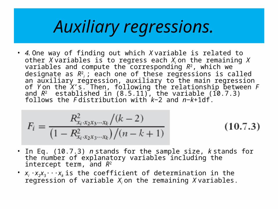
Auxiliary regressions. • 4. One way of finding out which X variable is related to other X

variables is to regress each Xi on the remaining X variables and compute the corresponding R2, which we designate as R2

i ; each one of these regressions is called an auxiliary regression, auxiliary to the main regression of Y on the X’s. Then, following the relationship between F and R2 established in (8.5.11), the variable (10.7.3) follows the F distribution with k−2 and n−k+1df.

• In Eq. (10.7.3) n stands for the sample size, k stands for the number of explanatory variables including the intercept term, and R2

• xi ·x2x3···xk is the coefficient of determination in the regression of variable Xi on the remaining X variables.

• If the computed F exceeds the critical Fi at the chosen level of significance, it is taken to mean that the particular Xi is collinear with other X’s; if it does not exceed the critical Fi, we say that it is not collinear with other X’s, in which case we may retain that variable in the model.

• Klien’s rule of thumb• Instead of formally testing all auxiliary R2 values, one may

adopt Klien’s rule of thumb, which suggests that multicollinearity may be a troublesome problem only if the R2 obtained from an auxiliary regression is greater than the overall R2, that is, that obtained from the regression of Y on all the regressors. Of course, like all other rules of thumb, this one should be used judiciously.

April 18, 2023 Slide 18

Tolerance and Variance Inflation Factors (VIFs)

• If the tolerance equals 1, the variables are unrelated. If TOLj = 0, then they are perfectly correlated.

• Variance Inflation Factors (VIFs)

• ToleranceV IF

R k

1

1 2

T O L R V IFj j j 1 12 ( / ( ))

April 18, 2023 Slide 19

Interpreting VIFs

• No multicollinearity produces VIFs = 1.0• If the VIF is greater than 10.0, then

multicollinearity is probably severe. 90% of the variance of Xj is explained by the other X’s.

• In small samples, a VIF of about 5.0 may indicate problems

Solution of Multicollinarity• 1. A priori information. • Suppose we consider the model • Yi = β1 + β2X2i + β3X3i + ui • where Y = consumption, X2 = income, and X3 = wealth. Suppose a

priori we believe that β3 = 0.10β2; that is, the rate of change of consumption with respect to wealth is one-tenth the corresponding rate with respect to income. We can then run the following regression:

• Yi = β1 + β2X2i + 0.10β2X3i + ui = β1 + β2Xi + ui

• where Xi = X2i + 0.1X3i . • Once we obtain βˆ2, we can estimate βˆ3 from the postulated

relationship between β2 and β3. How does one obtain a priori information? It could come from previous empirical work.

• 2. Combining cross-sectional and time series data.

• A variant of the priori information technique is the combination of cross-sectional and time-series data, known as pooling the data. Suppose we want to study the demand for automobiles in the US and assume we have time series data on the number of cars sold, average price of the car, and consumer income.

• Dropping the same variables

• Transformation of variables:

Additional or new data.

N = 10

N = 40