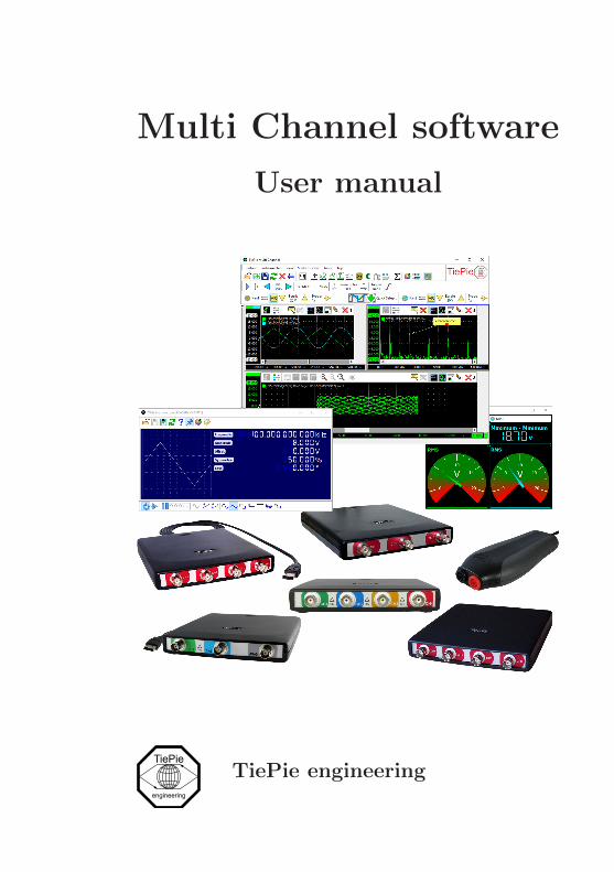
Multi Channel software

User manual

TiePie engineering

Copyright c©2017 TiePie engineering.All rights reserved.

Revision 1.07, March 2017

Despite the care taken for the compilation ofthis user manual, TiePie engineering can notbe held responsible for any damage resultingfrom errors that may appear in this manual.

Contents

1 Introduction 11.1 About the software . . . . . . . . . . . . . . . . . . . 11.2 How to use the software . . . . . . . . . . . . . . . . 2

1.2.1 Controlling the software . . . . . . . . . . . . 21.3 Software installation . . . . . . . . . . . . . . . . . . 31.4 Hardware installation . . . . . . . . . . . . . . . . . 3

2 Software basics 52.1 Main window parts . . . . . . . . . . . . . . . . . . . 52.2 Basic measurements . . . . . . . . . . . . . . . . . . 7

2.2.1 New graph . . . . . . . . . . . . . . . . . . . 82.2.2 Oscilloscope in Yt mode . . . . . . . . . . . . 82.2.3 Oscilloscope in XY mode . . . . . . . . . . . 82.2.4 Spectrum analyzer . . . . . . . . . . . . . . . 92.2.5 Transient recorder . . . . . . . . . . . . . . . 102.2.6 Voltmeter . . . . . . . . . . . . . . . . . . . . 112.2.7 CAN analyzer . . . . . . . . . . . . . . . . . . 122.2.8 I2C analyzer . . . . . . . . . . . . . . . . . . 122.2.9 Serial analyzer . . . . . . . . . . . . . . . . . 12

2.3 Printing . . . . . . . . . . . . . . . . . . . . . . . . . 132.4 Settings . . . . . . . . . . . . . . . . . . . . . . . . . 13

3 Displaying data 153.1 Graphs . . . . . . . . . . . . . . . . . . . . . . . . . . 15

3.1.1 Creating new graphs . . . . . . . . . . . . . . 153.1.2 Graph modes . . . . . . . . . . . . . . . . . . 163.1.3 Showing measured data in Yt mode . . . . . 173.1.4 Showing measured data in XY mode . . . . . 183.1.5 Drawing options . . . . . . . . . . . . . . . . 183.1.6 References . . . . . . . . . . . . . . . . . . . . 183.1.7 Cursors . . . . . . . . . . . . . . . . . . . . . 193.1.8 Axes . . . . . . . . . . . . . . . . . . . . . . . 21

3.2 Meters . . . . . . . . . . . . . . . . . . . . . . . . . . 23

4 Instruments 254.1 Controlling instruments . . . . . . . . . . . . . . . . 26

4.1.1 Instrument bar . . . . . . . . . . . . . . . . . 26

Contents I

4.1.2 Channel bar . . . . . . . . . . . . . . . . . . . 274.2 Settings . . . . . . . . . . . . . . . . . . . . . . . . . 27

4.2.1 Instrument settings . . . . . . . . . . . . . . . 284.2.2 Channel settings . . . . . . . . . . . . . . . . 31

4.3 Automatically storing measurements . . . . . . . . . 334.4 Streaming measurements . . . . . . . . . . . . . . . . 33

4.4.1 Streaming versus block measurements . . . . 344.4.2 Collecting streaming data . . . . . . . . . . . 344.4.3 Using streaming mode . . . . . . . . . . . . . 35

4.5 Combining instruments . . . . . . . . . . . . . . . . 35

5 Arbitrary Waveform Generator 375.1 Extended arbitrary waveform generator . . . . . . . 37

5.1.1 Toolbars . . . . . . . . . . . . . . . . . . . . . 385.1.2 Signal properties . . . . . . . . . . . . . . . . 395.1.3 Generator mode . . . . . . . . . . . . . . . . 395.1.4 Frequency mode . . . . . . . . . . . . . . . . 405.1.5 Sweep . . . . . . . . . . . . . . . . . . . . . . 40

5.2 Classic arbitrary waveform generator . . . . . . . . . 415.2.1 Toolbar . . . . . . . . . . . . . . . . . . . . . 425.2.2 Signal type . . . . . . . . . . . . . . . . . . . 425.2.3 Frequency . . . . . . . . . . . . . . . . . . . . 425.2.4 Symmetry . . . . . . . . . . . . . . . . . . . . 435.2.5 Amplitude . . . . . . . . . . . . . . . . . . . . 435.2.6 Offset . . . . . . . . . . . . . . . . . . . . . . 435.2.7 Output . . . . . . . . . . . . . . . . . . . . . 43

5.3 Setfiles . . . . . . . . . . . . . . . . . . . . . . . . . . 445.4 Arbitrary data . . . . . . . . . . . . . . . . . . . . . 44

5.4.1 Loading arbitrary data from a source . . . . . 445.4.2 Loading arbitrary data from a file . . . . . . 455.4.3 Data resampling . . . . . . . . . . . . . . . . 45

5.5 Hotkeys . . . . . . . . . . . . . . . . . . . . . . . . . 45

6 Objects 476.1 Using objects . . . . . . . . . . . . . . . . . . . . . . 476.2 Object tree . . . . . . . . . . . . . . . . . . . . . . . 486.3 Object types . . . . . . . . . . . . . . . . . . . . . . 486.4 Handling objects . . . . . . . . . . . . . . . . . . . . 49

6.4.1 Creating . . . . . . . . . . . . . . . . . . . . . 496.4.2 Cloning . . . . . . . . . . . . . . . . . . . . . 496.4.3 Connecting . . . . . . . . . . . . . . . . . . . 496.4.4 Disconnecting . . . . . . . . . . . . . . . . . . 50

II

6.4.5 Using aliases . . . . . . . . . . . . . . . . . . 516.5 Examples . . . . . . . . . . . . . . . . . . . . . . . . 52

6.5.1 Summing channel data . . . . . . . . . . . . . 526.5.2 Modulate measured data . . . . . . . . . . . 52

7 Sources 557.1 How to use sources . . . . . . . . . . . . . . . . . . . 557.2 Change unit . . . . . . . . . . . . . . . . . . . . . . . 557.3 Software signal generator . . . . . . . . . . . . . . . 557.4 Demo Source . . . . . . . . . . . . . . . . . . . . . . 56

8 I/Os 578.1 Gain/Offset . . . . . . . . . . . . . . . . . . . . . . . 578.2 Add/Subtract . . . . . . . . . . . . . . . . . . . . . . 588.3 Multiply/Divide . . . . . . . . . . . . . . . . . . . . 588.4 Sqrt . . . . . . . . . . . . . . . . . . . . . . . . . . . 588.5 ABS . . . . . . . . . . . . . . . . . . . . . . . . . . . 598.6 Differentiate . . . . . . . . . . . . . . . . . . . . . . . 598.7 Integrate . . . . . . . . . . . . . . . . . . . . . . . . . 608.8 Log . . . . . . . . . . . . . . . . . . . . . . . . . . . . 608.9 Low-pass filter . . . . . . . . . . . . . . . . . . . . . 618.10 Average . . . . . . . . . . . . . . . . . . . . . . . . . 618.11 Min/Max detector . . . . . . . . . . . . . . . . . . . 618.12 Limiter . . . . . . . . . . . . . . . . . . . . . . . . . 628.13 Resampler . . . . . . . . . . . . . . . . . . . . . . . . 628.14 Data collector . . . . . . . . . . . . . . . . . . . . . . 638.15 FFT . . . . . . . . . . . . . . . . . . . . . . . . . . . 648.16 Duty cycle . . . . . . . . . . . . . . . . . . . . . . . . 648.17 RPM-detector . . . . . . . . . . . . . . . . . . . . . . 658.18 Pulse decoder . . . . . . . . . . . . . . . . . . . . . . 668.19 CAN analyzer . . . . . . . . . . . . . . . . . . . . . . 678.20 SAE J1939 decoder . . . . . . . . . . . . . . . . . . . 68

9 Sinks 699.1 Meter . . . . . . . . . . . . . . . . . . . . . . . . . . 699.2 Table . . . . . . . . . . . . . . . . . . . . . . . . . . . 699.3 Disk writer . . . . . . . . . . . . . . . . . . . . . . . 70

9.3.1 File names . . . . . . . . . . . . . . . . . . . 719.3.2 Limiting file size . . . . . . . . . . . . . . . . 729.3.3 Skipping data . . . . . . . . . . . . . . . . . . 739.3.4 File type options . . . . . . . . . . . . . . . . 73

9.4 I2C Analyzer . . . . . . . . . . . . . . . . . . . . . . 73

Contents III

9.5 Serial analyzer . . . . . . . . . . . . . . . . . . . . . 749.6 Sound . . . . . . . . . . . . . . . . . . . . . . . . . . 749.7 Compression test . . . . . . . . . . . . . . . . . . . . 75

10 Files 7710.1 File types . . . . . . . . . . . . . . . . . . . . . . . . 77

10.1.1 Multi Channel TPS files . . . . . . . . . . . . 7710.1.2 Multi Channel TPO files . . . . . . . . . . . . 7810.1.3 WinSoft files . . . . . . . . . . . . . . . . . . 78

10.2 Saving Files . . . . . . . . . . . . . . . . . . . . . . . 7910.2.1 Saving to a TPS file . . . . . . . . . . . . . . 7910.2.2 Saving objects to a TPO file . . . . . . . . . 79

10.3 Loading Files . . . . . . . . . . . . . . . . . . . . . . 8110.3.1 Loading a whole file . . . . . . . . . . . . . . 8110.3.2 Loading just a part of a file . . . . . . . . . . 8110.3.3 Loading into selected objects . . . . . . . . . 82

10.4 Exporting data . . . . . . . . . . . . . . . . . . . . . 8310.4.1 How to export data . . . . . . . . . . . . . . 8310.4.2 Supported file types . . . . . . . . . . . . . . 85

A Standard measurements 87A.1 Short description of the measurements . . . . . . . . 88

B Hotkeys 93

C Command line parameters 97

Index 99

IV

Introduction 1The Multi Channel software package is the measuring soft-ware for the TiePie engineering measuring instruments andfunction generators. This document explains the basic func-tionality in the application. It is intended to get you startedand to teach you how to do basic and more advanced mea-surements.

A basic knowledge of controlling windows based applica-tions and computer based measuring instruments is assumed.For a detailed and up to date description of functionalityand objects that are not described in this document, referto the help file that comes with the Multi Channel softwareor to the classroom section of the TiePie engineering websitewww.tiepie.nl.

1.1 About the software

The Multi Channel software can control an unlimited amountof measuring instruments, each with an unlimited amount ofchannels. The Multi Channel software can display this datain an unlimited amount of different displays. Measured datacan be displayed directly, but it can also be processed first.

In addition to measured data from the instrument inputchannels, the software can also work with other data sources.For example data from internal software signal generators canbe combined with the measured data.

Besides for measuring and displaying data, the MultiChannel software can be used to control Arbitrary Wave-form Generators (AWG). An AWG can be used to generatestandard signals, like sine, block and triangle or for generat-ing arbitrary signals, for example signals that have previouslybeen measured. Refer to chapter 5 for information about theAWG.

Introduction 1

1.2 How to use the software

The Multi Channel software is suitable both for experiencedand inexperienced users. For performing basic measurementsin an easy way, you can use the quick functions, which areexplained in section 2.2. The quick functions automaticallycreate graphs and other objects that are needed to performthe measurement. To easily perform more complex measure-ments, you can load predefined setfiles and start measuringright away.

To get more control and flexibility, you can create objectsyourself and connect them to each other the way you want.You can find information about using objects in chapter 6and the online help. When you have created your test setup,you can store it in a setfile for later use. See chapter 10 formore information about using files.

1.2.1 Controlling the software

There are many different ways to control the Multi Channelsoftware. A few of them are treated in this section. This willbe enough to get you started. Not all of the functionalityis mentioned in this manual. Once you are used to how thesoftware is controlled, you will discover it yourself.

Hotkeys The instruments and graphs in the Multi Channelsoftware can be controlled with hotkeys. You can find a com-plete list of the hotkeys in appendix B. Once you know themost important hotkeys by heart you will be able to changesettings very quickly.

Popup menus Almost all settings and options in the MultiChannel software are available via popup menus. When youright-click an object, a popup menu will appear which con-tains actions that affect the object you clicked. The best wayto find all the possibilities is to try.

2 Chapter 1

Drag and drop Besides the popup menus, drag and dropis very important. You can drag different objects onto eachother or onto graphs to make connections and you can draggraph axes and trigger symbols. You can find more informa-tion about connecting different objects in section 6.4.3. Insection 3.1.8 you can read how to drag axes and trigger sym-bols. Just like with the popup menus, the best way to findall the possibilities is to try. The mouse cursor will indicatewhere the object you are dragging can be dropped.

1.3 Software installation

If you have just recently purchased your instrument, you canuse the installation program from the CD that comes withyour instrument to install the software. Otherwise it is recom-mended to download the latest version from www.tiepie.nl,because the Multi Channel software is constantly updated.With the latest version you will be able to use all functiona-lity of your hardware.

The installation process is straightforward and is not ex-plained in detail here. During the installation you will beprompted if you would like to associate the file extensions.DAT and .SET with the Multi Channel software. Thesefiles are used by the old WinSoft measurement software. Ifyou associate the extensions with the Multi Channel software(default), you will be able to open WinSoft files by just dou-ble clicking them or dragging them on the main window ofthe Multi Channel software. If you don’t have WinSoft filesor have other programs that use these file extensions, you canuncheck the checkboxes.

1.4 Hardware installation

Before the Multi Channel software can control your instru-ment(s), a driver needs to be installed. Please refer to the

Introduction 3

user manual of your instrument(s) for instructions for in-stalling hardware and drivers.

The drivers for the TiePie engineering instruments arecontinuously improved. It is recommended to downloadthe latest version of the driver for your instrument fromwww.tiepie.nl.

4 Chapter 1

Software basics 2This chapter will explain the basics of the Multi Channelsoftware to get you started. It will show you the differentparts of the main window and how to use them to performbasic measurements. A Handyscope HS5 is used in most ofthe examples, but of course other instruments supported bythe Multi Channel software can be used just as well.

2.1 Main window parts

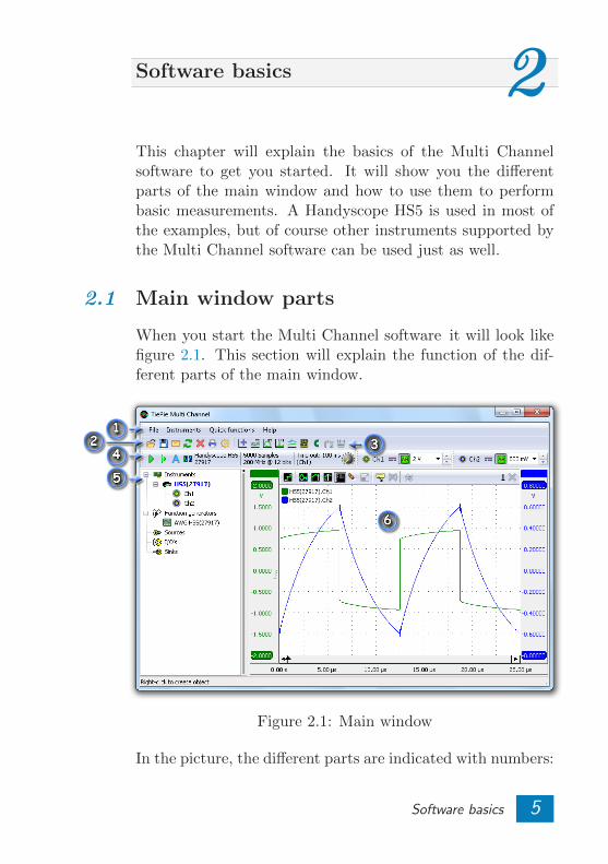
When you start the Multi Channel software it will look likefigure 2.1. This section will explain the function of the dif-ferent parts of the main window.

Figure 2.1: Main window

In the picture, the different parts are indicated with numbers:

Software basics 5

1 Main menu

2 File toolbar

3 Quick functions toolbar

4 Instrument toolbar

5 Object tree

6 Graph

File toolbar The file toolbar can be used for accessing fre-quently used items from the file menu, for example opening,saving or reloading files.

Quick functions toolbar The quick functions toolbarcontains quick functions to use the active measurement in-strument as a standard virtual instrument: oscilloscope,spectrum analyzer, transient recorder or voltmeter. The ac-tive instrument is the instrument highlighted in the objecttree. You can make another instrument active by clicking onit in the object tree or using the hotkey CTRL-n , with n aninstrument number (1..0). See section 2.2 for more informa-tion about the quick functions.

Instrument toolbar The instrument toolbar can be usedto control basic instrument settings, like sample frequency,record length and trigger settings. For each channel, a toolbaris present to control channel settings like range, auto rangingand coupling. Refer to chapter 4 for more information aboutcontrolling instruments.

Object tree The object tree is situated at the left side ofthe main window of the application. It contains the measur-ing instruments, function generators and other objects con-structed in the application. These other objects are datasources, I/O blocks and data sinks, which all can be used incombination with the measured data. Data of all sources canbe exported to different file types, see section 10.4.

6 Chapter 2

You can create a new source, I/O or sink by right click-ing on the label in the object tree and select the object ofyour choice from the popup menu. With drag and drop, thedifferent objects in the object tree can be connected to otherobjects. You can drag a source object on a sink object, I/Oblock or a graph. When the source is dropped it will con-nect the object it was dropped on. For detailed informationon how to work with the objects in the object tree, refer tochapter 6.2.

Graph The Multi Channel software allows you to createand arrange multiple graphs for displaying measured or ge-nerated data. In section 3.1 you can read more about graphs.

2.2 Basic measurements

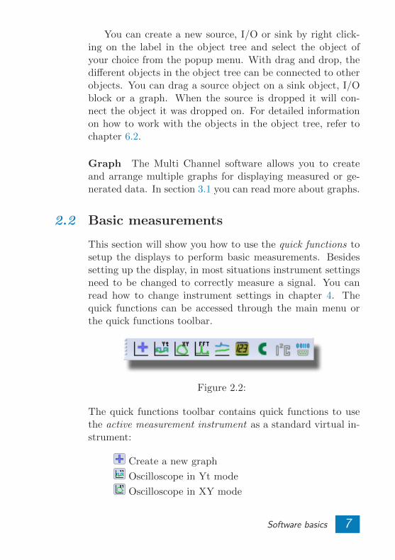
This section will show you how to use the quick functions tosetup the displays to perform basic measurements. Besidessetting up the display, in most situations instrument settingsneed to be changed to correctly measure a signal. You canread how to change instrument settings in chapter 4. Thequick functions can be accessed through the main menu orthe quick functions toolbar.

Figure 2.2:

The quick functions toolbar contains quick functions to usethe active measurement instrument as a standard virtual in-strument:

Create a new graph

Oscilloscope in Yt mode

Oscilloscope in XY mode

Software basics 7

Spectrum analyzer

Transient recorder

Voltmeter

CAN analyzer

I2C analyzer

Serial analyzer

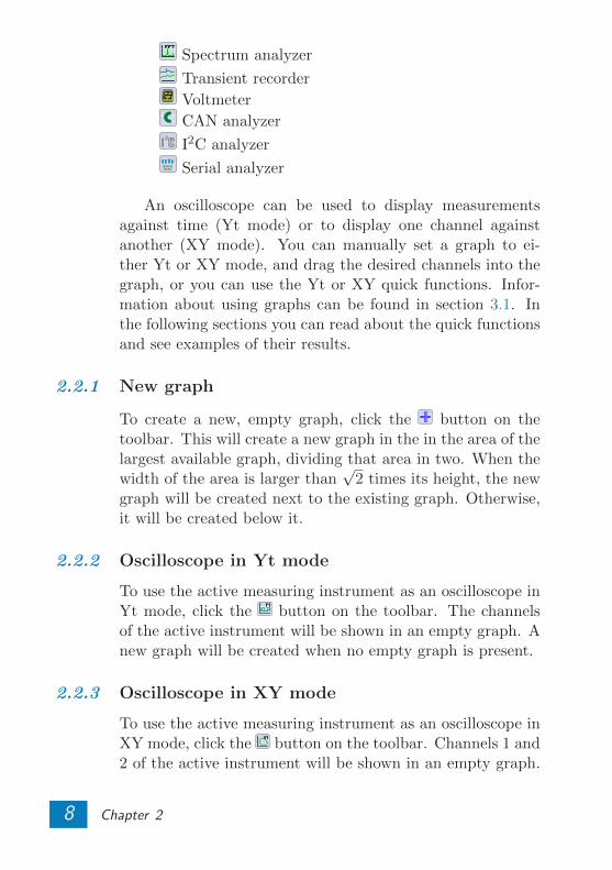
An oscilloscope can be used to display measurementsagainst time (Yt mode) or to display one channel againstanother (XY mode). You can manually set a graph to ei-ther Yt or XY mode, and drag the desired channels into thegraph, or you can use the Yt or XY quick functions. Infor-mation about using graphs can be found in section 3.1. Inthe following sections you can read about the quick functionsand see examples of their results.

2.2.1 New graph

To create a new, empty graph, click the button on thetoolbar. This will create a new graph in the in the area of thelargest available graph, dividing that area in two. When thewidth of the area is larger than

√2 times its height, the new

graph will be created next to the existing graph. Otherwise,it will be created below it.

2.2.2 Oscilloscope in Yt mode

To use the active measuring instrument as an oscilloscope inYt mode, click the button on the toolbar. The channelsof the active instrument will be shown in an empty graph. Anew graph will be created when no empty graph is present.

2.2.3 Oscilloscope in XY mode

To use the active measuring instrument as an oscilloscope inXY mode, click the button on the toolbar. Channels 1 and2 of the active instrument will be shown in an empty graph.

8 Chapter 2

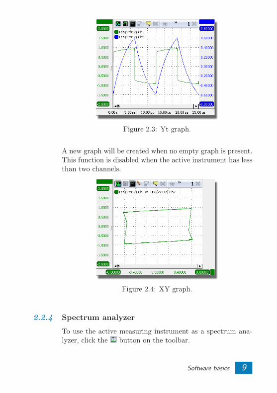
Figure 2.3: Yt graph.

A new graph will be created when no empty graph is present.This function is disabled when the active instrument has lessthan two channels.

Figure 2.4: XY graph.

2.2.4 Spectrum analyzer

To use the active measuring instrument as a spectrum ana-lyzer, click the button on the toolbar.

Software basics 9

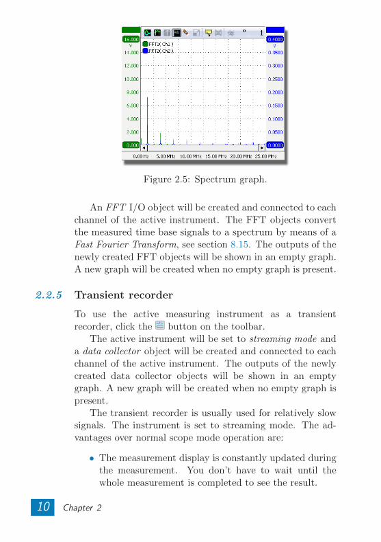
Figure 2.5: Spectrum graph.

An FFT I/O object will be created and connected to eachchannel of the active instrument. The FFT objects convertthe measured time base signals to a spectrum by means of aFast Fourier Transform, see section 8.15. The outputs of thenewly created FFT objects will be shown in an empty graph.A new graph will be created when no empty graph is present.

2.2.5 Transient recorder

To use the active measuring instrument as a transientrecorder, click the button on the toolbar.

The active instrument will be set to streaming mode anda data collector object will be created and connected to eachchannel of the active instrument. The outputs of the newlycreated data collector objects will be shown in an emptygraph. A new graph will be created when no empty graph ispresent.

The transient recorder is usually used for relatively slowsignals. The instrument is set to streaming mode. The ad-vantages over normal scope mode operation are:

• The measurement display is constantly updated duringthe measurement. You don’t have to wait until thewhole measurement is completed to see the result.

10 Chapter 2

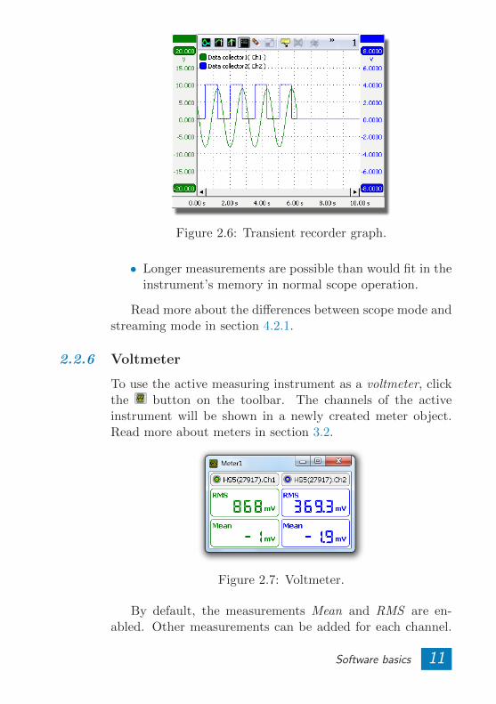
Figure 2.6: Transient recorder graph.

• Longer measurements are possible than would fit in theinstrument’s memory in normal scope operation.

Read more about the differences between scope mode andstreaming mode in section 4.2.1.

2.2.6 Voltmeter

To use the active measuring instrument as a voltmeter, clickthe button on the toolbar. The channels of the activeinstrument will be shown in a newly created meter object.Read more about meters in section 3.2.

Figure 2.7: Voltmeter.

By default, the measurements Mean and RMS are en-abled. Other measurements can be added for each channel.

Software basics 11

Examples are: minimum, maximum, top-bottom, variance,standard deviation, frequency and for frequency data: To-tal Harmonic Distortion. See appendix A for a list of theavailable measurements and a description.

2.2.7 CAN analyzer

To use the active measuring instrument as a CAN analyzer,click the button on the toolbar. A new CAN analyzer I/Owill be created and connected to an newly created table sinkto display the decoded CAN data. Read more on the CANanalyzer in section 8.19.

If the active instrument has two or more channels, theuser is asked whether one or two channels should be used.When two channels are used, both the CAN high and CANlow signal should be measured. The difference signal H-L iscalculated with a Add/Subtract I/O and fed into the analyzer.

If only one channel is used, this may measure CAN high,or the differential CAN signal H-L. The latter is only possiblewith a differential input.

2.2.8 I2C analyzer

To use the active measuring instrument as a I2C analyzer,click the button on the toolbar. A new I2C analyzer sinkwill be created and connected to the first two channels of theactive instrument. The I2C analyzer can only be used withinstruments with two or more channels. The first channelwill be used as I2C SCL (clock) and the second as I2C SDA(data). Read more on the I2C analyzer in section 9.4.

2.2.9 Serial analyzer

To use the active measuring instrument as a serial analyzer,click the button on the toolbar. A new Serial analyzersink will be created and connected to the first active channelof the active instrument. It can be used to analyze RS232,

12 Chapter 2

RS485, MIDI, DMX or other compatible serial buses. Readmore on the serial analyzer in section 9.5.

2.3 Printing

You can print your measurements just like they are shown onthe screen. Each graph is printed to a separate page. ChoosePrint... in the file menu, press the print button on the filetoolbar, or use the hotkey CTRL-P .

The graphs are printed with the selected graph scheme.By default a black and white printing scheme is used, butyou can also use a scheme with colors or define your owncolor scheme. You can select another scheme or change colorsfor printing in the application settings, in Graph→Print. Tocheck how the graphs will look on paper without actuallyprinting them, click Print preview... in the file menu.

2.4 Settings

Several applications settings can be changed with the settingswindow. You can open the settings window by clicking theSettings... item in the file menu or pressing the settingsbutton ( ) on the file toolbar.

All settings are stored in an INI file. This makes it possi-ble to easily backup your settings or to copy them to anothercomputer. You can also use another INI file. If you createan INI file with the same name as the application executablein some folder and run the Multi Channel software from thatfolder, that file will be used instead of the default one in theapplication folder. You can easily accomplish this by chang-ing the ”Start in” property of a shortcut.

Language The user interface of the Multi Channel soft-ware can be set to many different languages via the Setlanguage... item in the file menu. This item is always dis-played in English to make it easily accessible.

Software basics 13

Graph schemes You will notice the colors of the screenshots in this manual are different than the standard colorson your screen when you use the software. The screen shotswere made using a different graph scheme. You can choosefrom several schemes or make your own schemes for on screenas well as for printing.

Meter schemes Just as the colors of the graphs, the colorsof the meters can also be changed with schemes.

Toolbars The instument and channel toolbars (see sections4.1.1 and 4.1.2) are fully customizable. Buttons and read-outs for all settings can be dragged on or off the toolbar tomeet specific needs. Also the icon size and text size can beadjusted. Toolbar configurations can be stored for easy re-configuring different setups.

14 Chapter 2

Displaying data 3Measured or generated data can be displayed in differentways. Mostly graphs are used, but you can also use meters.This chapter will show you how to use graphs and meters.

3.1 Graphs

The Multi Channel software allows you to create and arrangegraphs the way you want. New graphs can be created on themain screen of the Multi Channel software and can be movedto a separate window outside the main screen.

3.1.1 Creating new graphs

Creating new graphs is very easy: Simply click the new graphquick function button . This will create a new graph in thein the area of the largest available graph, dividing that areain two. When the width of the area is larger than

√2 times

its height, the new graph will be created next to the existinggraph. Otherwise, it will be created below it.

It is also possible to create a graph at a self defined loca-tion. 1 Right-click anywhere in a graph on the main screenand select Make new graph from the menu. 2 After drag-ging a rectangle anywhere on the graph section, a new graphwill be created on the selected position. See figure 3.1.

The size of the newly created graph can be adjusted bydragging the edges of the graph. When the mouse cursor ismoved over the edges of a graph, the mouse cursor will changeshape to indicate that the size of the graph can be changed.

Displaying data 15

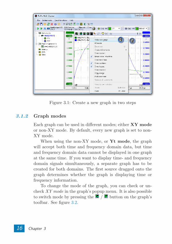
Figure 3.1: Create a new graph in two steps

3.1.2 Graph modes

Each graph can be used in different modes; either XY modeor non-XY mode. By default, every new graph is set to non-XY mode.

When using the non-XY mode, or Yt mode, the graphwill accept both time and frequency domain data, but timeand frequency domain data cannot be displayed in one graphat the same time. If you want to display time- and frequencydomain signals simultaneously, a separate graph has to becreated for both domains. The first source dragged onto thegraph determines whether the graph is displaying time orfrequency information.

To change the mode of the graph, you can check or un-check XY mode in the graph’s popup menu. It is also possibleto switch mode by pressing the / button on the graph’stoolbar. See figure 3.2.

16 Chapter 3

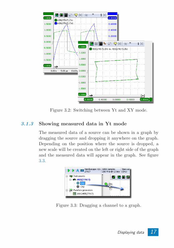
Figure 3.2: Switching between Yt and XY mode.

3.1.3 Showing measured data in Yt mode

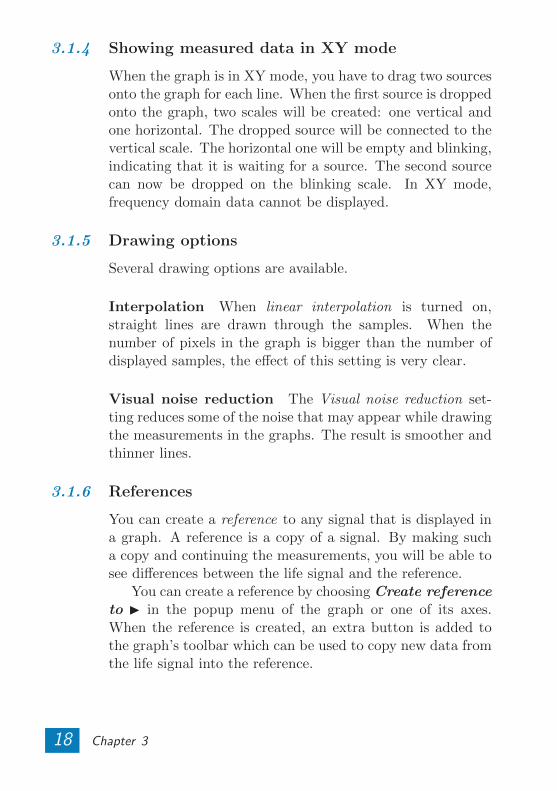
The measured data of a source can be shown in a graph bydragging the source and dropping it anywhere on the graph.Depending on the position where the source is dropped, anew scale will be created on the left or right side of the graphand the measured data will appear in the graph. See figure3.3.

Figure 3.3: Dragging a channel to a graph.

Displaying data 17

3.1.4 Showing measured data in XY mode

When the graph is in XY mode, you have to drag two sourcesonto the graph for each line. When the first source is droppedonto the graph, two scales will be created: one vertical andone horizontal. The dropped source will be connected to thevertical scale. The horizontal one will be empty and blinking,indicating that it is waiting for a source. The second sourcecan now be dropped on the blinking scale. In XY mode,frequency domain data cannot be displayed.

3.1.5 Drawing options

Several drawing options are available.

Interpolation When linear interpolation is turned on,straight lines are drawn through the samples. When thenumber of pixels in the graph is bigger than the number ofdisplayed samples, the effect of this setting is very clear.

Visual noise reduction The Visual noise reduction set-ting reduces some of the noise that may appear while drawingthe measurements in the graphs. The result is smoother andthinner lines.

3.1.6 References

You can create a reference to any signal that is displayed ina graph. A reference is a copy of a signal. By making sucha copy and continuing the measurements, you will be able tosee differences between the life signal and the reference.

You can create a reference by choosing Create referenceto I in the popup menu of the graph or one of its axes.When the reference is created, an extra button is added tothe graph’s toolbar which can be used to copy new data fromthe life signal into the reference.

18 Chapter 3

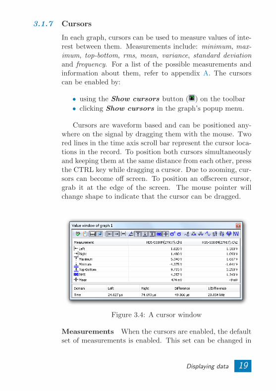
3.1.7 Cursors

In each graph, cursors can be used to measure values of inte-rest between them. Measurements include: minimum, max-imum, top-bottom, rms, mean, variance, standard deviationand frequency. For a list of the possible measurements andinformation about them, refer to appendix A. The cursorscan be enabled by:

• using the Show cursors button ( ) on the toolbar

• clicking Show cursors in the graph’s popup menu.

Cursors are waveform based and can be positioned any-where on the signal by dragging them with the mouse. Twored lines in the time axis scroll bar represent the cursor loca-tions in the record. To position both cursors simultaneouslyand keeping them at the same distance from each other, pressthe CTRL key while dragging a cursor. Due to zooming, cur-sors can become off screen. To position an offscreen cursor,grab it at the edge of the screen. The mouse pointer willchange shape to indicate that the cursor can be dragged.

Figure 3.4: A cursor window

Measurements When the cursors are enabled, the defaultset of measurements is enabled. This set can be changed in

Displaying data 19

Settings→Graph→Value window→Measurements. The cur-sor window will look like figure 3.4.

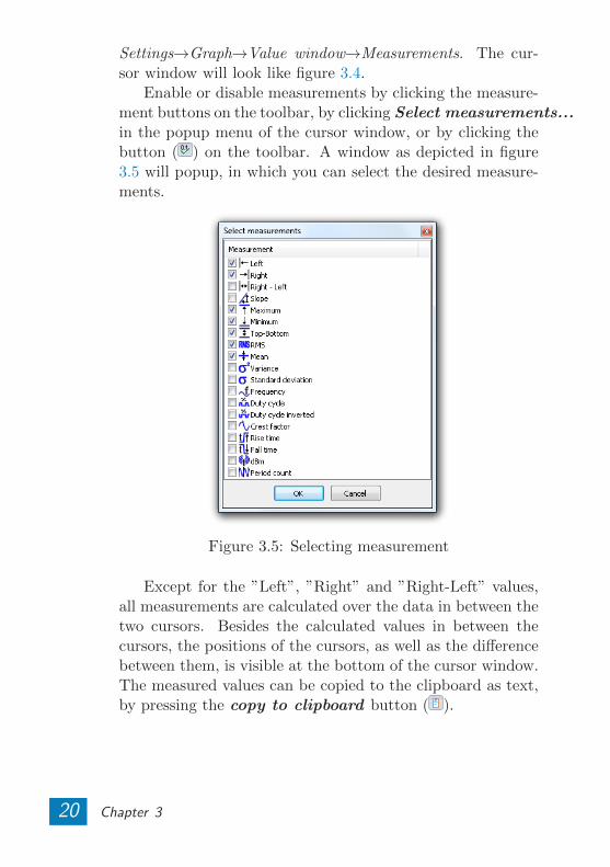
Enable or disable measurements by clicking the measure-ment buttons on the toolbar, by clicking Select measurements...in the popup menu of the cursor window, or by clicking thebutton ( ) on the toolbar. A window as depicted in figure3.5 will popup, in which you can select the desired measure-ments.

Figure 3.5: Selecting measurement

Except for the ”Left”, ”Right” and ”Right-Left” values,all measurements are calculated over the data in between thetwo cursors. Besides the calculated values in between thecursors, the positions of the cursors, as well as the differencebetween them, is visible at the bottom of the cursor window.The measured values can be copied to the clipboard as text,by pressing the copy to clipboard button ( ).

20 Chapter 3

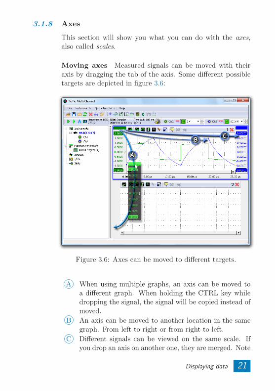
3.1.8 Axes

This section will show you what you can do with the axes,also called scales.

Moving axes Measured signals can be moved with theiraxis by dragging the tab of the axis. Some different possibletargets are depicted in figure 3.6:

Figure 3.6: Axes can be moved to different targets.

A When using multiple graphs, an axis can be moved toa different graph. When holding the CTRL key whiledropping the signal, the signal will be copied instead ofmoved.

B An axis can be moved to another location in the samegraph. From left to right or from right to left.

C Different signals can be viewed on the same scale. Ifyou drop an axis on another one, they are merged. Note

Displaying data 21

that the units of the axes must be the same. You canextract a signal from an axis by choosing Extract linefrom its popup menu.

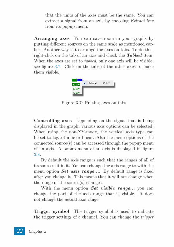
Arranging axes You can save room in your graphs byputting different sources on the same scale as mentioned ear-lier. Another way is to arrange the axes on tabs. To do this,right-click on the tab of an axis and check the Tabbed item.When the axes are set to tabbed, only one axis will be visible,see figure 3.7. Click on the tabs of the other axes to makethem visible.

Figure 3.7: Putting axes on tabs

Controlling axes Depending on the signal that is beingdisplayed in the graph, various axis options can be selected.When using the non-XY-mode, the vertical axis type canbe set to logarithmic or linear. Also the menu options of theconnected source(s) can be accessed through the popup menuof an axis. A popup menu of an axis is displayed in figure3.8.

By default the axis range is such that the ranges of all ofits sources fit in it. You can change the axis range to with themenu option Set axis range.... By default range is fixedafter you change it. This means that it will not change whenthe range of the source(s) changes.

With the menu option Set visible range... you canchange the part of the axis range that is visible. It doesnot change the actual axis range.

Trigger symbol The trigger symbol is used to indicatethe trigger settings of a channel. You can change the trigger

22 Chapter 3

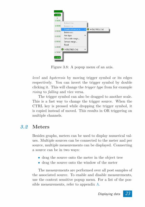
Figure 3.8: A popup menu of an axis.

level and hysteresis by moving trigger symbol or its edgesrespectively. You can invert the trigger symbol by doubleclicking it. This will change the trigger type from for examplerising to falling and vice versa.

The trigger symbol can also be dragged to another scale.This is a fast way to change the trigger source. When theCTRL key is pressed while dropping the trigger symbol, itis copied instead of moved. This results in OR triggering onmultiple channels.

3.2 Meters

Besides graphs, meters can be used to display numerical val-ues. Multiple sources can be connected to the meter and persource, multiple measurements can be displayed. Connectinga source can be in two ways:

• drag the source onto the meter in the object tree

• drag the source onto the window of the meter

The measurements are performed over all post samples ofthe associated source. To enable and disable measurements,use the context sensitive popup menu. For a list of the pos-sible measurements, refer to appendix A.

Displaying data 23

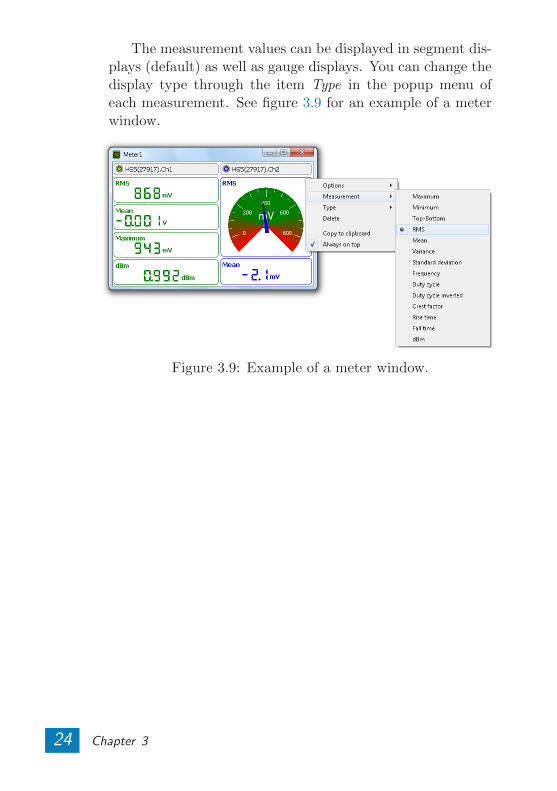
The measurement values can be displayed in segment dis-plays (default) as well as gauge displays. You can change thedisplay type through the item Type in the popup menu ofeach measurement. See figure 3.9 for an example of a meterwindow.

Figure 3.9: Example of a meter window.

24 Chapter 3

Instruments 4

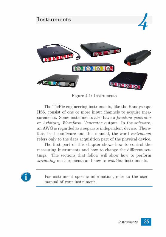
Figure 4.1: Instruments

The TiePie engineering instruments, like the HandyscopeHS5, consist of one or more input channels to acquire mea-surements. Some instruments also have a function generatoror Arbitrary Waveform Generator output. In the software,an AWG is regarded as a separate independent device. There-fore, in the software and this manual, the word instrumentrefers only to the data acquisition part of the physical device.

The first part of this chapter shows how to control themeasuring instruments and how to change the different set-tings. The sections that follow will show how to performstreaming measurements and how to combine instruments.

For instrument specific information, refer to the usermanual of your instrument.

Instruments 25

4.1 Controlling instruments

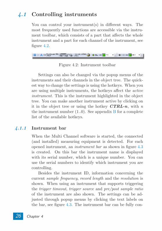
You can control your instrument(s) in different ways. Themost frequently used functions are accessible via the instru-ment toolbar, which consists of a part that affects the wholeinstrument and a part for each channel of the instrument, seefigure 4.2.

Figure 4.2: Instrument toolbar

Settings can also be changed via the popup menus of theinstruments and their channels in the object tree. The quick-est way to change the settings is using the hotkeys. When youare using multiple instruments, the hotkeys affect the activeinstrument. This is the instrument highlighted in the objecttree. You can make another instrument active by clicking onit in the object tree or using the hotkey CTRL-n , with nthe instrument number (1..0). See appendix B for a completelist of the available hotkeys.

4.1.1 Instrument bar

When the Multi Channel software is started, the connected(and installed) measuring equipment is detected. For eachopened instrument, an instrument bar as shown in figure 4.3is created. On this bar the instrument name is displayedwith its serial number, which is a unique number. You canuse the serial numbers to identify which instrument you arecontrolling.

Besides the instrument ID, information concerning thecurrent sample frequency, record length and the resolution isshown. When using an instrument that supports triggeringthe trigger timeout, trigger source and pre/post sample ratioof the instrument are also shown. The settings can be ad-justed through popup menus by clicking the text labels onthe bar, see figure 4.3. The instrument bar can be fully con-

26 Chapter 4

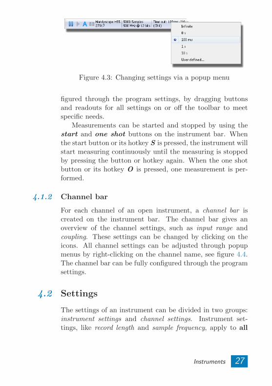
Figure 4.3: Changing settings via a popup menu

figured through the program settings, by dragging buttonsand readouts for all settings on or off the toolbar to meetspecific needs.

Measurements can be started and stopped by using thestart and one shot buttons on the instrument bar. Whenthe start button or its hotkey S is pressed, the instrument willstart measuring continuously until the measuring is stoppedby pressing the button or hotkey again. When the one shotbutton or its hotkey O is pressed, one measurement is per-formed.

4.1.2 Channel bar

For each channel of an open instrument, a channel bar iscreated on the instrument bar. The channel bar gives anoverview of the channel settings, such as input range andcoupling. These settings can be changed by clicking on theicons. All channel settings can be adjusted through popupmenus by right-clicking on the channel name, see figure 4.4.The channel bar can be fully configured through the programsettings.

4.2 Settings

The settings of an instrument can be divided in two groups:instrument settings and channel settings. Instrument set-tings, like record length and sample frequency, apply to all

Instruments 27

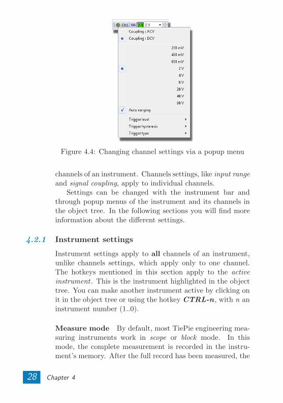
Figure 4.4: Changing channel settings via a popup menu

channels of an instrument. Channels settings, like input rangeand signal coupling, apply to individual channels.

Settings can be changed with the instrument bar andthrough popup menus of the instrument and its channels inthe object tree. In the following sections you will find moreinformation about the different settings.

4.2.1 Instrument settings

Instrument settings apply to all channels of an instrument,unlike channels settings, which apply only to one channel.The hotkeys mentioned in this section apply to the activeinstrument . This is the instrument highlighted in the objecttree. You can make another instrument active by clicking onit in the object tree or using the hotkey CTRL-n , with n aninstrument number (1..0).

Measure mode By default, most TiePie engineering mea-suring instruments work in scope or block mode. In thismode, the complete measurement is recorded in the instru-ment’s memory. After the full record has been measured, the

28 Chapter 4

data is transferred to the computer. The next measurementis started after the data has been processed, therefore thereare gaps between the measurements.

Besides working in block mode TiePie engineering instru-ments support working in streaming mode. In this modethe measured data is transferred directly to the computer,without using the internal memory of the instrument. Thismakes it possible to perform continuous measurements with-out gaps. For more information on streaming measurements,refer to section 4.4. You can change the measure mode of aninstrument via its popup menu in the object tree.

To change the measure mode of an instrument, the in-strument must first be set to pause.

Sample frequency The sample frequency is the rate atwhich the instrument takes its samples of the input signals.It can be set to predefined or user defined values via differentmenus. Use the hotkeys F3 and F4 to decrease or increasethe sample frequency.

Record length The record length is the number of samplesthe instrument takes during each measurement or record. Itcan be set to predefined or user defined values via differentmenus. Use the hotkeys F11 and F12 to decrease or increasethe record length.

Resolution The resolution of an instrument determinesthe smallest voltage step that can be detected. The resolu-tion is indicated with a number of bits. Every extra bit dou-bles the accuracy. This means that the smallest detectablevoltage step will be 16 times smaller when you use a 12 bitresolution instead of 8 bit. You can change the resolution ofan instrument via its popup menu in the object tree.

Instruments 29

Pre-trigger In most cases, all samples in the record willbe measured after a trigger. It is however also possible tomeasure a part of the record before the trigger moment.The samples taken before the trigger moment are called pre-samples. The remaining samples are called post-samples.You can change the pre/post-sample ratio with the knob onthe instrument bar and via different menus or with hotkeysSHIFT + ← and SHIFT + →.

When measuring fast periodical signals, in most casesnot all pre-samples will be measured. This is becausethe trigger condition is met before all pre-samples havebeen measured and starts the post-sample counter.You will see the first pre-samples are zero when theyare not measured.

Trigger time-out The trigger time-out is an often over-looked, but important setting. When the measurement isstarted, the instrument will start waiting for the trigger event.When the trigger event does not occur within the time-outtime, the instrument starts measuring the post-samples au-tomatically. This will not result in a stable display, but itwill give an impression of the signal. This will enable you tochange the trigger settings to accomplish stable triggering.Use the hotkeys 0 , 1 and W to change the time-out to 0, 1second or infinite respectively.

When the instrument should measure only when a trig-ger event occurs the trigger time-out must be set toinfinite!

Trigger source The trigger source setting of an instrumentdetermines which trigger signals are used to trigger the mea-

30 Chapter 4

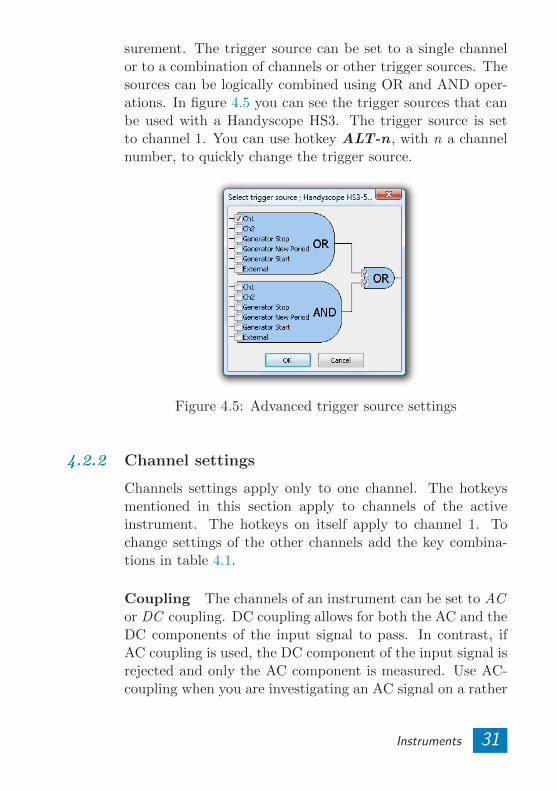
surement. The trigger source can be set to a single channelor to a combination of channels or other trigger sources. Thesources can be logically combined using OR and AND oper-ations. In figure 4.5 you can see the trigger sources that canbe used with a Handyscope HS3. The trigger source is setto channel 1. You can use hotkey ALT-n , with n a channelnumber, to quickly change the trigger source.

Figure 4.5: Advanced trigger source settings

4.2.2 Channel settings

Channels settings apply only to one channel. The hotkeysmentioned in this section apply to channels of the activeinstrument. The hotkeys on itself apply to channel 1. Tochange settings of the other channels add the key combina-tions in table 4.1.

Coupling The channels of an instrument can be set to ACor DC coupling. DC coupling allows for both the AC and theDC components of the input signal to pass. In contrast, ifAC coupling is used, the DC component of the input signal isrejected and only the AC component is measured. Use AC-coupling when you are investigating an AC signal on a rather

Instruments 31

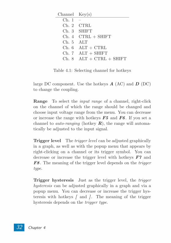
Channel Key(s)

Ch. 1 –Ch. 2 CTRLCh. 3 SHIFTCh. 4 CTRL + SHIFTCh. 5 ALTCh. 6 ALT + CTRLCh. 7 ALT + SHIFTCh. 8 ALT + CTRL + SHIFT

Table 4.1: Selecting channel for hotkeys

large DC component. Use the hotkeys A (AC) and D (DC)to change the coupling.

Range To select the input range of a channel, right-clickon the channel of which the range should be changed andchoose input voltage range from the menu. You can decreaseor increase the range with hotkeys F5 and F6 . If you set achannel to auto-ranging (hotkey R), the range will automa-tically be adjusted to the input signal.

Trigger level The trigger level can be adjusted graphicallyin a graph, as well as with the popup menu that appears byright-clicking on a channel or its trigger symbol. You candecrease or increase the trigger level with hotkeys F7 andF8 . The meaning of the trigger level depends on the triggertype.

Trigger hysteresis Just as the trigger level, the triggerhysteresis can be adjusted graphically in a graph and via apopup menu. You can decrease or increase the trigger hys-teresis with hotkeys [ and ] . The meaning of the triggerhysteresis depends on the trigger type.

32 Chapter 4

Trigger type A different trigger type can be selected perchannel. Depending on the trigger type, the input signal ismonitored differently. Examples of trigger types are risingand falling slope and In- and OutWindow. Refer to theonline help for a detailed description of the trigger types.

4.3 Automatically storing measurements

You can use the auto disk function to automatically storeall measurements. This is particularly useful when you aremeasuring an event that occurs sporadically. When you setthe trigger settings such that the instrument will trigger whenthe event occurs and use the auto disk function, all events willbe stored.

To enable auto disk, click AutoDisk... in the instru-ments menu. A save dialog will show, in which you can en-ter a filename. A rising number will be appended to thisfilename for each measurement. For example, naming thefiles TiePie will create a file sequence of TiePie000000.TPS,TiePie000001.TPS, etc.

4.4 Streaming measurements

By default, TiePie engineering measuring instruments workin scope or block mode. In this mode, the complete measure-ment is recorded in the instrument’s memory. After the fullrecord has been measured, the data is transferred to the com-puter. The next measurement is started after the data hasbeen processed, therefore there are gaps between the mea-surements.

Besides working in block mode TiePie engineering instru-ments support working in streaming mode. In this modethe measured data is transferred directly to the computer,without using the internal memory of the instrument. Thismakes it possible to perform continuous measurements with-out gaps.

Instruments 33

4.4.1 Streaming versus block measurements

Both block and streaming measurements have their advan-tages and disadvantages. The key features of both modes arelisted below. Block mode (/Scope mode):

+ Fast measurements are possible

− Record length is limited by the instrument’s memorysize

Stream mode:

+ Long measurements are possible

− Sample speed is limited by the data transfer rate tocomputer and the computer speed

In block mode, the next measurement is started after theprevious data has been transferred to the computer. Thismeans that there will always be a (small) gap in betweenthe measurements. In streaming mode, no data is missed.All successive data blocks can be connected to form one bigmeasurement.

A disadvantage of the streaming mode is that the maxi-mum measurement speed depends on the data transfer ratefrom the instrument to the computer and on the overall sys-tem performance.

4.4.2 Collecting streaming data

In streaming mode, successive measurements will arrive inblocks. Each of those blocks contains record length samplesand can be connected seamlessly with previous and next datablocks.

The Data collector I/O-object can be used to collect thesuccessive measurements and combine them into one big blockof data of up to 20 million samples.

34 Chapter 4

4.4.3 Using streaming mode

By default, TiePie engineering measuring instruments workin scope or block mode. There are several ways to set aninstrument’s mode to stream.

The easiest way to use the streaming mode is to use oneof the quick functions: Transient recorder. When you choosethis function, either from the main menu or the toolbar, itwill set the selected instrument’s mode to stream. Besidesthis, for each channel of the instrument a data collector I/O-object is created with a data size of 100000 samples and eachdata collector is put into a graph.

To manually change the mode of an instrument, usethe popup menu of the instrument in the object tree. Inthe menu, select ”Measure mode→Stream” or ”Measuremode→Block”.

To change the measure mode, the instrument must firstbe set to pause.

4.5 Combining instruments

With the Multi Channel software, you are not limited tonumber of channels of one instrument. It is possible to com-bine two or more instruments to form a combined instrument.Once the instruments are combined, the resulting single in-strument works just like a normal instrument. There is nolimit to the number of channels in a combined instrument.At the time this manual is written, combining is possible withthe following instruments:

• Handyscope HS3

• Handyscope HS4

• Handyscope HS4 DIFF

• Handyscope HS5

Instruments 35

You can create a combined instrument by selecting Cre-ate combined instrument... from the Instrument menu.Choose which instruments must be combined in the appear-ing dialog.

The instruments must be synchronized with a couplingcable attached to their extension connectors.

36 Chapter 4

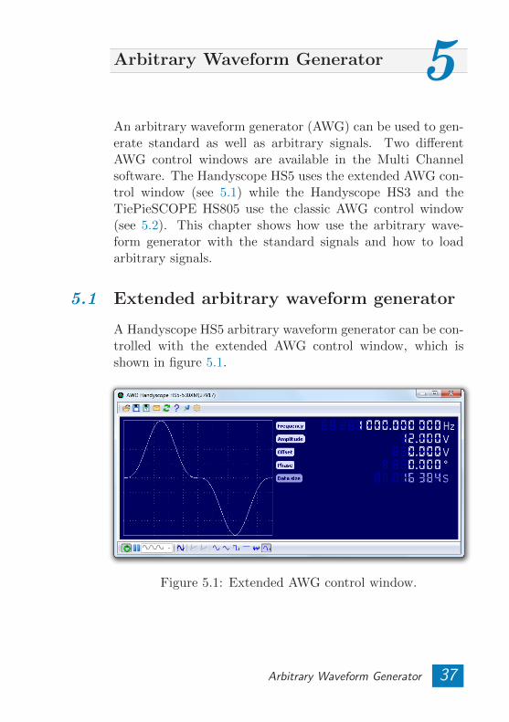
Arbitrary Waveform Generator 5An arbitrary waveform generator (AWG) can be used to gen-erate standard as well as arbitrary signals. Two differentAWG control windows are available in the Multi Channelsoftware. The Handyscope HS5 uses the extended AWG con-trol window (see 5.1) while the Handyscope HS3 and theTiePieSCOPE HS805 use the classic AWG control window(see 5.2). This chapter shows how use the arbitrary wave-form generator with the standard signals and how to loadarbitrary signals.

5.1 Extended arbitrary waveform generator

A Handyscope HS5 arbitrary waveform generator can be con-trolled with the extended AWG control window, which isshown in figure 5.1.

Figure 5.1: Extended AWG control window.

Arbitrary Waveform Generator 37

5.1.1 Toolbars

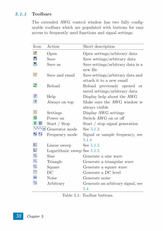
The extended AWG control window has two fully config-urable toolbars which are populated with buttons for easyaccess to frequently used functions and signal settings:

Icon Action Short description

Open Open settings/arbitrary data

Save Save settings/arbitrary data

Save as Save settings/arbitrary data in anew file

Save and email Save settings/arbitrary data andattach it to a new email

Reload Reload previously opened orsaved settings/arbitrary data

Help Display help about the AWG

Always on top Make sure the AWG window isalways visible

Settings Display AWG settings

Power on Switch AWG on or off

Start / Stop Start / stop signal generation

Generator mode See 5.1.3

Frequency mode Signal or sample frequency, see5.1.4

Linear sweep See 5.1.5

Logarithmic sweep See 5.1.5

Sine Generate a sine wave

Triangle Generate a triangular wave

Square Generate a square wave

DC Generate a DC level

Noise Generate noise

Arbitrary Generate an arbitrary signal, see5.4

Table 5.1: Toolbar buttons.

38 Chapter 5

5.1.2 Signal properties

Depending on the selected signal type and generator mode,various signal properties like frequency or amplitude can beset. To adjust a signal property, the property name label canbe clicked. This opens a dialog in which the new value canbe entered. This dialog accepts prefixes like u, m, k, M, etc.

Properties can also be adjusted by clicking the digits orscrolling the mouse wheel when the mouse pointer is over aspecific digit. Clicking the upper half of a digit will increasethe value of that digit, while clicking the lower half of a digitdecreases it. Digits that are currently off, can be enabled byclicking their upper half.

5.1.3 Generator mode

Generator mode can only be set when the generator is stopped.The following generator modes are supported:

Continuous When the start button is pressed,the signal generation is started and continues until stoppedby the user.

Burst When the start button is pressed, the sig-nal generation is started. It stops automatically after ’burstcount’ periods.

Gated periods After the start button is pressed,signal generation is started when an enabled external triggerinput becomes active. When the enabled external triggerinput(s) becomes inactive, the current period is finalized andsignal generation stops. A combination of any of the availabletrigger inputs can be used. When none are enabled, externaltrigger input 2 is automatically enabled when gated periodsis selected. (Note that the external trigger inputs are activeby default, unless pulled down.)

Arbitrary Waveform Generator 39

5.1.4 Frequency mode

Frequency mode determines the relation between the frequencycontrols and the output frequency. Available frequency modesare limited by the current signal type. The Handyscope HS5AWG frequency mode is fixed to signal frequency for signaltypes sine, triangle, square and DC, and to to sample fre-quency for signal type noise. Both modes can be used forarbitrary signals. The following frequency modes are sup-ported:

Signal frequency The frequency controls set the fre-quency at which the signal will be repeated.

Sample frequency The frequency controls set the sam-ple frequency at which the individual samples of the signalwill be generated.

5.1.5 Sweep

The sweep function enables a linear or logarithmic continuoussweep with the selected signal type (sine, triangle or square).The sweep runs from frequency1 to frequency2, where fre-quency1 is allowed to be higher than frequency2. Optionally,the sweep can start at a different frequency by setting thestart frequency to a value between the two sweep frequen-cies. Duration determines the sweep duration.

The accuracy of the sweep is determined by sweep set-tings in the settings dialog. The minimum and maximumnumber of samples that are used for one period of the signalcan be set, as well as the maximum amount of samples forthe complete sweep. Higher values will give a more accuratesweep, but changes to sweep properties will take a bit longerto take effect.

Sweeping is only available on Handyscope HS5 modelswith extended memory option XM.

40 Chapter 5

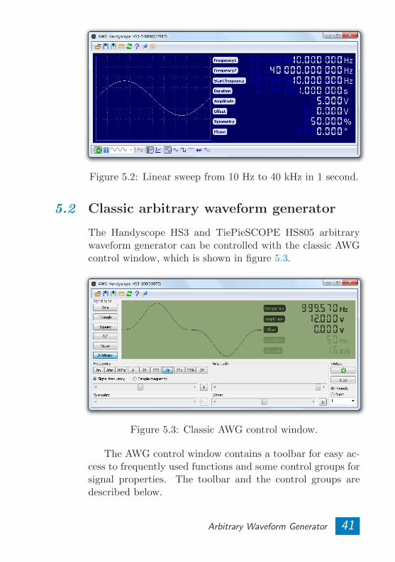
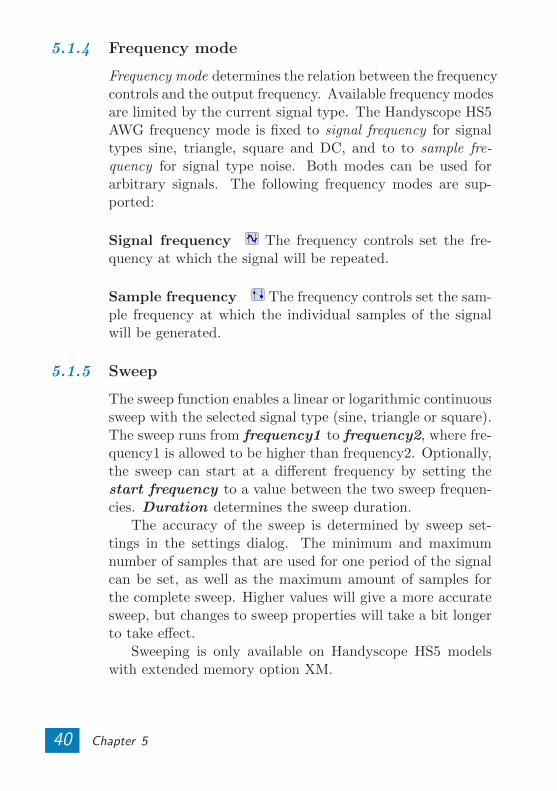
Figure 5.2: Linear sweep from 10 Hz to 40 kHz in 1 second.

5.2 Classic arbitrary waveform generator

The Handyscope HS3 and TiePieSCOPE HS805 arbitrarywaveform generator can be controlled with the classic AWGcontrol window, which is shown in figure 5.3.

Figure 5.3: Classic AWG control window.

The AWG control window contains a toolbar for easy ac-cess to frequently used functions and some control groups forsignal properties. The toolbar and the control groups aredescribed below.

Arbitrary Waveform Generator 41

5.2.1 Toolbar

The toolbar at the top of the window contains some buttonsfor easy access to frequently used functions. The function ofthe different buttons is described in table 5.1.

Icon Action Short description

Open Open settings/arbitrary data

Save Save settings/arbitrary data

Save as Save settings/arbitrary data in anew file

Save and email Save settings/arbitrary data andattach it to a new email

Reload Reload previously opened orsaved settings/arbitrary data

Help Display help about the AWG

Always on top Make sure the AWG window is al-ways visible

Table 5.2: Toolbar buttons.

5.2.2 Signal type

The different signal types supported by the AWG can beselected with buttons. The signal that will be at the outputof the generator is displayed. By default, no arbitrary data isloaded into the AWG. As a result only an offset is generatedwhen ’arbitrary’ is chosen. See section 5.4 for informationabout loading data.

5.2.3 Frequency

The frequency can be adjusted with the range select buttonsand the scroll bar. An exact frequency value can be enteredafter pressing the hotkey F or after double-clicking the fre-quency display. The actual value is shown on the display.

42 Chapter 5

By default, the signal frequency will be displayed. This isthe frequency at which the displayed signal will be repeated.It is also possible to change the sampling frequency of theAWG directly, by checking the sample frequency radio but-ton. The minimum and maximum frequency will depend onthe instrument.

5.2.4 Symmetry

The symmetry can be adjusted with the scroll bar. An exactsymmetry value can be entered after pressing the hotkey S orafter double-clicking the symmetry display. The actual valueis shown on the display. The symmetry range is 0% - 100%.

5.2.5 Amplitude

The amplitude can be adjusted with the scroll bar. An exactamplitude value can be entered after pressing the hotkey Aor after double-clicking the amplitude display. The actualvalue is shown on the display. The minimum and maximumamplitude will depend on the instrument.

5.2.6 Offset

The offset can be adjusted with the scroll bar. An exactoffset value can be entered after pressing the hotkey O orafter double-clicking the offset display. The actual value isshown on the display. The minimum and maximum offsetwill depend on the instrument.

5.2.7 Output

The two buttons in the output group can be used to turn theoutput on or off, and to start or stop the signal:

Turn AWG on/off.

Start/stop AWG signal output.

Arbitrary Waveform Generator 43

By default, the signal will output continuously, but it isalso possible to perform a burst of a certain number of periodsof the signal. To perform a burst, check the ”Burst” radiobutton and select or type the number of periods in the combobox. After pressing ”Start” the burst will be generated.

5.3 Setfiles

All settings and arbitrary data of the AWG can be saved insetfiles with the Save and Save as... buttons on the toolbar.Setfiles can be loaded with the Load... toolbar button, or bydragging a setfile onto the AWG control window. In figure5.3 for example, setfile Sin3.TPS is loaded, which contains anarbitrary signal (sine3). See chapter 10 for more informationabout using files.

5.4 Arbitrary data

Besides some standard signals, the arbitrary waveform gene-rator (AWG) can output arbitrary data. There are differentways of loading such data into the generator. Data can beloaded directly from an open source in the software, or froma file. See chapter 10 for more information about using files.

5.4.1 Loading arbitrary data from a source

Data of every source in the Multi Channel software can beloaded directly into an AWG. This means that measureddata, but also processed or generated data can be put intothe AWG. There are two ways to do this. One way is to dragthe source onto the AWG in the object tree. The other wayto get the data of a source is to drag the source onto a AWGcontrol window.

Note: Depending on the AWG and the data size, datamay be resampled during loading, see 5.4.3.

44 Chapter 5

5.4.2 Loading arbitrary data from a file

Besides loading data from a source, it can also be loaded froma file. Currently, loading data from TiePie engineering TPSfile and from Wave audio files is supported.

From a TiePie engineering TPS file, data can be read fromeach AWG or Source chunk in the file. Data from Wave audiofiles can also be read into the AWG. If more than one channel(mono) is available in the file, only the first channel will beread. All uncompressed Wave audio files with a resolution of8, 16, 32 or 64 bit are supported.

Note: Depending on the AWG and the data size, datamay be resampled during loading, see 5.4.3.

5.4.3 Data resampling

When loading data into an AWG, it is possible that the AWGdoes not support the data size of the loaded data. This canhappen for example when the data is too big to fit into thememory of the AWG. The Handyscope HS3 has another li-mitation: the data size must be a power of two (2, 4 , 8, 16,..., 262144).

When it is not possible to set the data size of the AWGto the data’s size, the data will be stretched or shrunken tofit exactly into the possible data size that is closest to therequested data size.

5.5 Hotkeys

The AWG can be controlled with several hotkeys, see ap-pendix B for a complete list.

Arbitrary Waveform Generator 45

46 Chapter 5

Objects 6The Multi Channel software can be used to do basic measure-ments that could also be done with a classic oscilloscope. Forsuch basic measurements, one graph displaying the measureddata is enough. In section 2.2 you can read how to performsuch basic measurements very easily.

Besides basic measurements, the Multi Channel softwareis capable of performing more complex processing on the mea-sured data. This processing is done with the help of differentobjects: sources, I/Os or processing blocks, and sinks. Thischapter will explain how to work with the different objects:how to create them and how to connect them to each other.At the end of the chapter you will find some examples insection 6.5.

6.1 Using objects

There are a lot of occasions where using objects is helpful dur-ing measurements. Sometimes you want to display the sumof different channels. You can do this with a Add/SubtractI/O object. Another example is power measurement. Whenyou measure the voltage over a load with one channel andthe current through it with another channel, you can mul-tiply the data of both channels with a Multiply/Divide I/Oobject to get the power.

You can also use a Low-pass filter to filter your measure-ments. The easiest way to learn about the possibilities of theobjects is to try. Just create some objects, connect them toeach other and see what happens. You can also have a lookat the examples in section 6.5 to get you started.

Objects 47

6.2 Object tree

The object tree is situated at the left side of the main windowof the application. It contains the measuring instruments,function generators and other objects constructed in the ap-plication, the data sources, I/O blocks and data sinks, whichall can be used in combination with the measured data.

Via the object tree, you can create different in- and out-put blocks (see section 6.4.1) and connect them (see sec-tion 6.4.3). When sources are connected to an object, thisis indicated by the caption of the object in the tree. Forexample when two channels of a Handyscope HS5 are con-nected to a Add/Subtract I/O object, its caption will changeto Add/Subtract1(HS5(27917).Ch1 + HS5(27917).Ch2). Youcan hide or show the object tree by pressing the symbols Jand I respectively.

You can export data to different file formats via the popupmenu of the sources (and I/Os) in the object tree. Read howto do this in section 10.4.

6.3 Object types

The different objects are divided into groups that are visiblein the object tree. Each group of objects is described in itsown chapter:

Instruments Chapter 4Function Generators Chapter 5Sources Chapter 7I/Os Chapter 8Sinks Chapter 9

Sources are objects that output data. This can be constantdata, like in the demo source, or any other kind of data. Themost important sources are the instrument channels.

48 Chapter 6

I/Os also called processing blocks are objects with input(s)and output(s). They produce data at their output(s) that issomehow related to their input(s). A Low pass filter I/O forexample filters the input data. The output of a processingblock is again a source, which can be connected to other I/Oblocks or to graphs.

Sinks are the opposite of a source. Instead of supplyingdata, they accept it, just like an I/O object. The differenceis that a sink does not have an output source.

6.4 Handling objects

6.4.1 Creating

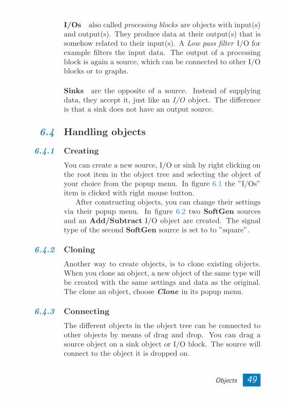
You can create a new source, I/O or sink by right clicking onthe root item in the object tree and selecting the object ofyour choice from the popup menu. In figure 6.1 the ”I/Os”item is clicked with right mouse button.

After constructing objects, you can change their settingsvia their popup menu. In figure 6.2 two SoftGen sourcesand an Add/Subtract I/O object are created. The signaltype of the second SoftGen source is set to to ”square”.

6.4.2 Cloning

Another way to create objects, is to clone existing objects.When you clone an object, a new object of the same type willbe created with the same settings and data as the original.The clone an object, choose Clone in its popup menu.

6.4.3 Connecting

The different objects in the object tree can be connected toother objects by means of drag and drop. You can drag asource object on a sink object or I/O block. The source willconnect to the object it is dropped on.

Objects 49

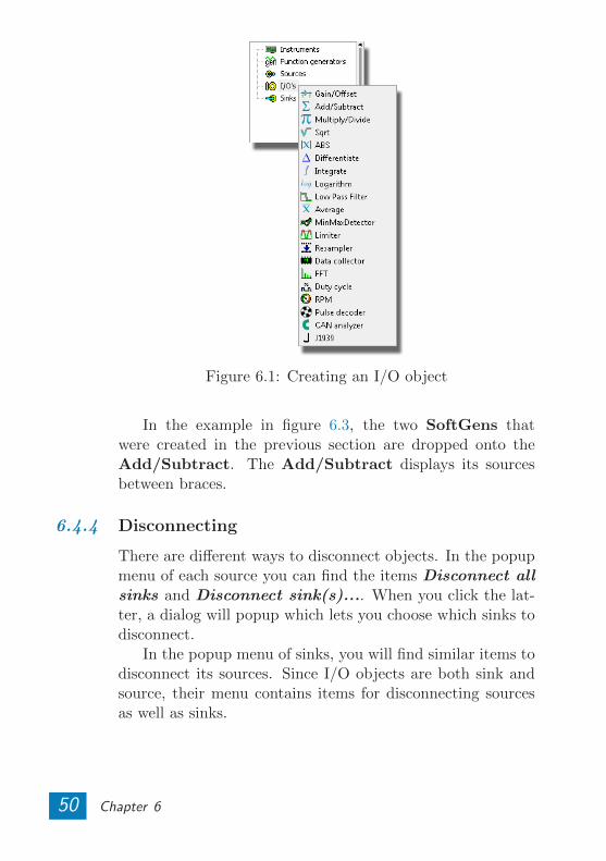
Figure 6.1: Creating an I/O object

In the example in figure 6.3, the two SoftGens thatwere created in the previous section are dropped onto theAdd/Subtract. The Add/Subtract displays its sourcesbetween braces.

6.4.4 Disconnecting

There are different ways to disconnect objects. In the popupmenu of each source you can find the items Disconnect allsinks and Disconnect sink(s).... When you click the lat-ter, a dialog will popup which lets you choose which sinks todisconnect.

In the popup menu of sinks, you will find similar items todisconnect its sources. Since I/O objects are both sink andsource, their menu contains items for disconnecting sourcesas well as sinks.

50 Chapter 6

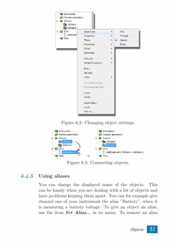
Figure 6.2: Changing object settings.

→Figure 6.3: Connecting objects.

6.4.5 Using aliases

You can change the displayed name of the objects. Thiscan be handy when you are dealing with a lot of objects andhave problems keeping them apart. You can for example givechannel one of your instrument the alias ”Battery”, when itis measuring a battery voltage. To give an object an alias,use the item Set Alias... in its menu. To remove an alias

Objects 51

and revert to the original name of the object, set the alias toan empty string.

6.5 Examples

In this section you will find some examples of how to usedifferent objects to process data.

6.5.1 Summing channel data

In some applications it is useful to sum or subtract the dataof different channels. To do this, create an Add/Subtractobject (right-click: Object tree→I/Os→Add/Subtract) anddrag the sources you want to add on top of it in the ob-ject tree. In figure 6.4 you can see the result of summingthe two channels of a Handyscope HS5. Note that it is dif-ficult to compare the different signals because they have dif-ferent scales. To make comparison easier, put the signals onone axis by dragging the axes on top of each other, see sec-tion 3.1.8. To subtract sources, change the +− mask of theAdd/Subtract object, see section 8.2 on page 58.

6.5.2 Modulate measured data

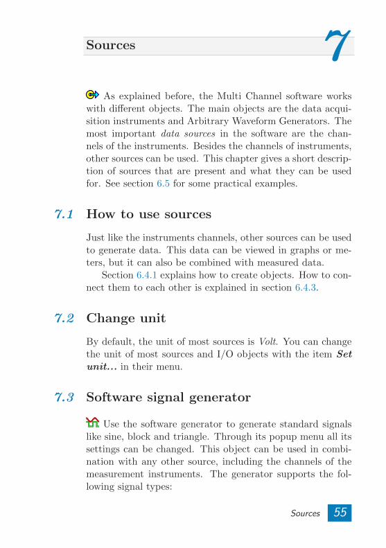
You can modulate measured data with a sine wave generatedby a software signal generator. Create a software signal ge-nerator (right-click: Object tree→Sources→SoftGen) and setits sample frequency and data size to the same values as yourinstrument. Then create a Multiply/Divide I/O object andconnect the signal generator and your measuring channel toit. The result of the Multiply/Divide is the measured data,multiplied with the generated data. In figure 6.5 you can seethe result in a graph.

52 Chapter 6

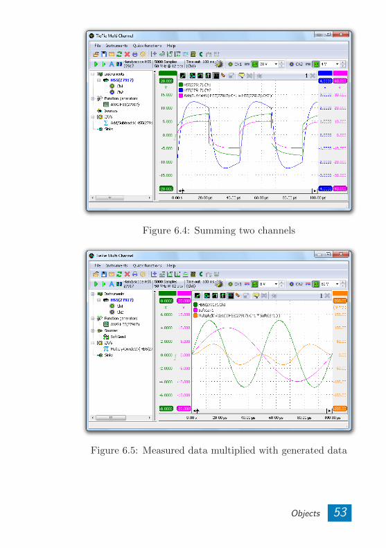
Figure 6.4: Summing two channels

Figure 6.5: Measured data multiplied with generated data

Objects 53

54 Chapter 6

Sources 7As explained before, the Multi Channel software works

with different objects. The main objects are the data acqui-sition instruments and Arbitrary Waveform Generators. Themost important data sources in the software are the chan-nels of the instruments. Besides the channels of instruments,other sources can be used. This chapter gives a short descrip-tion of sources that are present and what they can be usedfor. See section 6.5 for some practical examples.

7.1 How to use sources

Just like the instruments channels, other sources can be usedto generate data. This data can be viewed in graphs or me-ters, but it can also be combined with measured data.

Section 6.4.1 explains how to create objects. How to con-nect them to each other is explained in section 6.4.3.

7.2 Change unit

By default, the unit of most sources is Volt. You can changethe unit of most sources and I/O objects with the item Setunit... in their menu.

7.3 Software signal generator

Use the software generator to generate standard signalslike sine, block and triangle. Through its popup menu all itssettings can be changed. This object can be used in combi-nation with any other source, including the channels of themeasurement instruments. The generator supports the fol-lowing signal types:

Sources 55

• Sine

• Triangle

• Square

• Noise

Several signal parameters can be adjusted:

• Signal frequency

• Phase

• Amplitude

• Offset

• Symmetry

• Data size

• Sample frequency

7.4 Demo Source

The demo source contains a little bit of data, which isonly meant for demonstration. There are two different datasets from which one is chosen depending on the number (evenor odd) of the demo source.

Try creating two demo sources and add them to an emptygraph. If you set the graph to XY-mode you can see thepurpose of the demo data. You can read how to view data ina graph in section 3.1.

56 Chapter 7

I/Os 8I/Os, also called processing blocks are objects with in-

put(s) and output(s). They produce data at their output(s)that is somehow related to their input(s). For example, a Lowpass filter I/O filters the input data and a FFT I/O convertsthe input data to a frequency spectrum. The output(s) of theI/Os can be used as sources for further processing. This chap-ter will give an overview of I/O objects in the Multi Channelsoftware. Refer to the online help for more complete and upto date information.

8.1 Gain/Offset

Use the Gain/Offset I/O to multiply a signal with a cer-tain factor and to add an offset. It is mostly used in com-bination with sensors. For example, if you are measuringwith an acceleration sensor which produces 167 mV/g, youcan convert the measured voltage to g ’s with a gain factor of1/0.167 = 5.99. Note that you do not have to calculate this.You can enter this value directly as ”1/0.167” or ”1/167m”.

To invert a source, you can use a Gain/Offset I/O witha gain of -1.

You can enter the offset in two ways: at the input or atthe output. In the example with the accelerometer, you cansubtract the component caused by gravity in two ways: enteran input offset of -167 mV, or enter an output offset of -1 g.

When the source of the Gain/Offset I/O is a spectrum,you can use the Spectrum to density setting to convert amagnitude spectrum into a density spectrum. For exampleif the unit of the source spectrum is V, the output unit willbecome V/Hz.

I/Os 57

The Gain/Offset I/O can also be used to neutralize anoffset in a signal.

8.2 Add/Subtract

Use the Add/Subtract object to add or subtract the data ofdifferent sources. The +− mask determines which sources areadded and which sources are subtracted. This mask containsa + or − character for every connected source. By default,the mask consists of +-es only and all sources are added. Tosubtract a source, set its corresponding mask character to −.For example, to subtract sources 2 and 3 from source 1, setthe mask to ”+ − −”. Up to 32 sources can be added orsubtracted with an Add/Subtract I/O. See section 6.5.1 foran example of using the Add/Subtract I/O object.

8.3 Multiply/Divide

Use the Multiply/Divide object to multiply or divide thedata of different sources. Depending on the */ mask, theinput sources can be either in the nominator (default) or thedenominator. This mask works similar to the mask of theAdd/Subtract I/O. For example, a mask of ”*//” will resultin src1/(src2*src3). A maximum of 32 sources can be used.

A typical application of the Multiply/Divide object ispower measurement. When you measure the voltage over aload and the current through it, you can calculate the powerby multiplying both measurements.

8.4 Sqrt

The Sqrt processing block calculates the square root ofeach sample of the source’s data.

58 Chapter 8

The Sqrt-I/O can be used to calculate RMS values.Perform the following steps:

• Create a multiply/divide

• Create a low pass filter

• Create a Sqrt

• Drag your source onto the multiply/divide twiceto calculate squared values of the source’s data.

• Drag the multiply/divide onto the low pass filterto calculate a running mean of the squares.

• Drag the low pass filter onto the Sqrt to get theRMS values.

8.5 ABS

Use this processing block to take the absolute value of allsamples of its source. The ABS operation does the followingfor every sample:

if sample < 0 then sample := -sample;

8.6 Differentiate

Use this processing block to differentiate data. The out-put is proportional to rate of change of the input. For ex-ample, if a source has the unit Volt, the output of the DIFFwill have unit Volt/s. The output range can be changed andfixed to user defined values.

I/Os 59

The differentiate operation is very sensitive to noise,because in most cases noise has a higher frequency thanthe signal of interest. To minimize the effect of noise,add a low-pass filter processing block before or afterthe differentiate block.

8.7 Integrate

The Integrate processing block is the inverse of the Dif-ferentiate operation. The output range of the integrate pro-cessing block can also be changed and fixed.

An ideal integrator integrates all frequencies in a signal.In practice, unwanted offsets can cause problems with anideal integrator. Therefore the integrate object contains aleakage parameter. In its menu you can set the Leak fre-quency. All frequencies below the leak frequency will besuppressed.

If you are using acceleration sensors, you can integratetheir acceleration signal to obtain the speed. Integra-tion of the speed will give the relative position.

8.8 Log

The Logarithm processing block calculates the logarithmof the input data. The base number that is used is selectablefrom 2, e, 10 and user defined. Additionally a gain can beset.

60 Chapter 8

8.9 Low-pass filter

Use this processing block to filter data. Data is filteredwith a first order low-pass IIR filter. The cut-off frequencycan be entered through its popup menu. The filtered data canbe multiplied by a gain which can also be entered throughthe popup menu.

8.10 Average

Averaging is useful in situations when the signal of inte-rest is periodic and (random) noise is present on top of it.By taking multiple measurements of the signal and averagingthem, the signal to noise ratio will increase.

The average I/O object can work in two different modes:running average (default) and average-of-n. When the ob-ject is working in running average mode, it will continuouslyreplace a part of its memory by the newly arriving data,effectively ”forgetting” the oldest measurements. In average-of-n mode, the average will automatically be cleared after nmeasurements. You can manually clear the average with theClear option in its menu.

8.11 Min/Max detector

Use the Min/Max detector to detect minimum or max-imum values of a source. By default maximum values arebe detected. Every time the source of the Min/Max detec-tor signals new data, the detector will compare each value inmemory to the new source data and keep the largest value.Minima can be detected instead of maxima by choosing Min-imum in the popup menu.

Optionally a fall-off percentage can be set. If this per-centage is not zero, the output will slowly fall back to theinput signal. The higher the fall-off percentage, the faster

I/Os 61

the memory values of the detector will fall in the direction ofthe source values. The effect can be compared to a VU-meterwith peak detect.

When only expand is set, the data size of the Min/Maxdetector gets higher when the source’s data size grows, butdoes not shrink when the source’s data does. This can beuseful when detecting minima or maxima of a source withvarying data size.

8.12 Limiter

Use this processing block to limit or clip a signal to acertain range. The clip range can be set via the popup menuof the limiter. The limiter works as follows: all values of thesignal above the maximum of the clip range are changed tothe maximum value. All values below the minimum of theclip range are changed to the minimum value.

if sample < ClipMin then sample := ClipMin elseif sample > ClipMax then sample := ClipMax;

8.13 Resampler

Use the Resampler processing block to change the sam-ple frequency (and record length) of a signal. This can beuseful when several signals are sampled with a high samplefrequency but not all of them require this high speed. Withthe resampler, the signal(s) that can be represented with alower sample frequency, can be resampled to a lower samplefrequency.

An example: when using a RPM I/O to determine thespeed of an engine, the sample frequency must be around10 kHz or higher to get the accurate rpms. Once the speedhas been determined, it can be resampled to a lower samplefrequency, for example 10 Hz, because the speed will vary

62 Chapter 8

relatively slow. This decreases the amount a memory ( or filesize ) by a factor 1000.

You can enter the ratio between output sample frequencyand input sample frequency directly via the resampler’s popupmenu. It is also possible to enter the output sample fre-quency in the menu. In that case, the ratio is calculatedautomatically.

Different resampling methods are available:

• normal: The input data is sampled at the output sam-ple times without any interpolation.

• linear: The linear interpolated input data is sampledat the output sample times.

• average: When the ratio is smaller than 1, the meanvalue of several samples of the input data is used foreach output sample. When the ratio is greater than 1,the linear method is used.

8.14 Data collector

Use the data collector object when performing streamingmeasurements. During streaming measurements, data arrivesin blocks with a size equal to the instrument’s record length.To form a continuous stream of data, these blocks must beappended to each other. The data collector does this job. Itwill fill its data with the arriving blocks of data.

The size of the collected data can be set to a maximum of20 million samples. When the data collector is full, differentactions can be performed:

• Continue: the oldest data is shifted out at the left, whilenew data is appended to the right

• Stop: data collecting is stopped when full. (The mea-surement is NOT stopped.)

• Clear: the output data is cleared and the filling startsover again

I/Os 63

• Overwrite: existing data in the output array is over-written by the new data

8.15 FFT

Use the FFT I/O object for spectral analysis of a signal.The FFT object converts a time base signal to a spectrum bymeans of a Fast Fourier Transform, an efficient algorithm tocompute the Discrete Fourier transform (DFT). As describedin section 3.1.2, the output of an FFT I/O can be connectedto a graph with a frequency scale or an empty graph.

The Fast Fourier Transform treats the input signal as if itwas a periodical signal. In other words, it assumes the signalis an infinitely long series of repetitions of the record. In prac-tice, mostly the record does not contain an integer numberof periods of the signal. Therefore, if the end of the record isconnected to the beginning, a discontinuity will arise, whichresults in extra frequency components in the resulting spec-trum. This effect is called spectral leakage.

To minimize the effect of spectral leakage, the inputrecord of the FFT can be multiplied with a window. Thisis called windowing. Several windows can be chosen in themenu of the FFT I/O, which all basically perform the sameaction: they make the edges of the record smoother to makethe discontinuities smaller. In most cases, the Blackman-Harris window will give the best results. However, if yourdata contains an integer number of periods, the rectangle (nowindowing) will give the best result. Refer to the online helpfor more information.

8.16 Duty cycle

Use the Duty cycle processing block to determine theduty cycle of a signal. Normally the duty cycle is defined asthe ratio between the time that a signal is higher than half

64 Chapter 8

the amplitude and the period. It is usually expressed as apercentage.

In some applications, for example in automotive applica-tions, it is more convenient to invert the percentage, such that”low” means active. Select Type→Inverted in the popupmenu to use it.

By default the mid-level is automatically detected, ashalfway between the minimum and the maximum of the in-put signal. In most applications this will give good results.However, when a signal is noisy or inactive, it can lead towrong duty cycle detection. To prevent this from happening,it is possible to set the mid-level via the popup menu.

8.17 RPM-detector

In modern engines, usually a crankshaft sensor is presentwhich generates a periodic signal with a number of periodsper revolution of the engine. The RPM block can be used toconvert this signal into revolutions per minute. The enginespeed is calculated multiple times per revolution. Because ofthis, variations in the engine speed during a revolution arevisible.

In figure 8.1 you can see a crank shaft signal of a truckduring start-up, which is converted to the engine speed withan RPM block. The middle picture is a zoomed in part ofthe top picture.

Gaps are present in a typical crankshaft signal. The sig-nal can for example consist of three times eighteen periods ofa sine-like signal and a two period gap per revolution, whichresults in sixty periods per revolution. This is the default set-ting of the RPM-detector. The gaps are detected internallyby the RPM block and the number of RPMs is only detectedbetween each period of the sine wave.

The number of periods per revolution of the used enginecan be entered through the popup menu of the RPM block.As well as the maximum detectable RPM.

I/Os 65

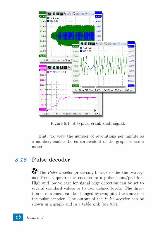
Figure 8.1: A typical crank shaft signal.

Hint: To view the number of revolutions per minute asa number, enable the cursor readout of the graph or use ameter.

8.18 Pulse decoder

The Pulse decoder processing block decodes the two sig-nals from a quadrature encoder to a pulse count/position.High and low voltage for signal edge detection can be set toseveral standard values or to user defined levels. The direc-tion of movement can be changed by swapping the sources ofthe pulse decoder. The output of the Pulse decoder can beshown in a graph and in a table sink (see 9.2).

66 Chapter 8

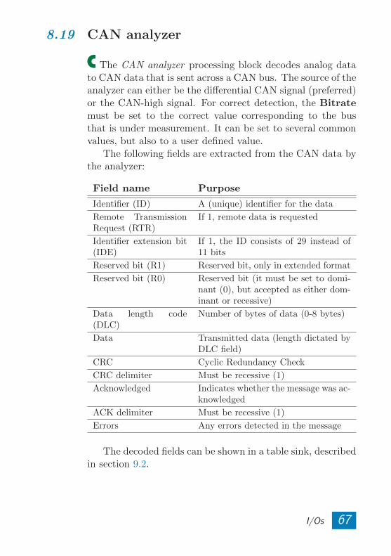
8.19 CAN analyzer

The CAN analyzer processing block decodes analog datato CAN data that is sent across a CAN bus. The source of theanalyzer can either be the differential CAN signal (preferred)or the CAN-high signal. For correct detection, the Bitratemust be set to the correct value corresponding to the busthat is under measurement. It can be set to several commonvalues, but also to a user defined value.

The following fields are extracted from the CAN data bythe analyzer:

Field name Purpose

Identifier (ID) A (unique) identifier for the data

Remote TransmissionRequest (RTR)

If 1, remote data is requested

Identifier extension bit(IDE)

If 1, the ID consists of 29 instead of11 bits

Reserved bit (R1) Reserved bit, only in extended format

Reserved bit (R0) Reserved bit (it must be set to domi-nant (0), but accepted as either dom-inant or recessive)

Data length code(DLC)

Number of bytes of data (0-8 bytes)

Data Transmitted data (length dictated byDLC field)

CRC Cyclic Redundancy Check

CRC delimiter Must be recessive (1)

Acknowledged Indicates whether the message was ac-knowledged

ACK delimiter Must be recessive (1)

Errors Any errors detected in the message

The decoded fields can be shown in a table sink, describedin section 9.2.

I/Os 67

8.20 SAE J1939 decoder

The J1939 decoder I/O (or J1939 analyzer) extracts SAEJ1939 SPN values from CAN messages. It has one input thatmust be connected to a source of CAN messages, typically aCAN analyzer I/O (see 8.19), and can have multiple outputs.Each output contains the values of a single SPN (SuspectParameter Number), selected from a database or loaded froma custom INI file. The data from these outputs can be used ingraphs, meter sinks, table sinks and by other I/Os. TypicalSPNs are:

• Engine coolant temperature

• Engine intake manifold temperature

• Engine speed

• Engine oil level

• etc.

J1939 is a high-level protocol that defines the communi-cation between nodes or electronic control units on a vehicleCAN bus. It was developed by the Society of AutomotiveEngineers (SAE) for car and heavy duty truck applications.Currently the J1939 standard is used worldwide by heavyduty truck and machinery companies. J1939 is commonlyused for communications throughout a vehicle or machine.

68 Chapter 8

Sinks 9Besides sources and processing blocks, the Multi Chan-

nel software also contains sinks. Sinks are the opposite of asource. Instead of supplying data, they accept it, just likean I/O object. The difference is that a sink does not havean output source. An example of a sink is a meter object,which displays certain measurements on the input data. Thischapter will give an overview of the sink objects. Refer to theonline help for more up to date information.

9.1 Meter

Use the Meter sink to view numerical values. A descrip-tion of the functionality is given in chapter 3.2

9.2 Table

Use the table sink to view values in a grid. You canconnect a source by dragging it onto:

• the table in the object tree

• the window of the table

The values contained in the source’s data are displayedin multiple columns. The table can display both numericaland string values. Columns can be hidden via the columnheader popup menu. Sort the grid values by clicking on acolumn header.

A table with decoded data from a CAN bus, decoded bya CAN analyzer I/O (see 8.19) is shown in figure 9.1.

Sinks 69

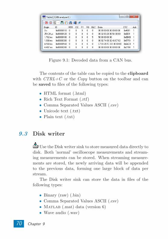
Figure 9.1: Decoded data from a CAN bus.

The contents of the table can be copied to the clipboardwith CTRL+C or the Copy button on the toolbar and canbe saved to files of the following types:

• HTML format (.html)

• Rich Text Format (.rtf)

• Comma Separated Values ASCII (.csv)

• Unicode text (.txt)

• Plain text (.txt)

9.3 Disk writer

Use the Disk writer sink to store measured data directly todisk. Both ’normal’ oscilloscope measurements and stream-ing measurements can be stored. When streaming measure-ments are stored, the newly arriving data will be appendedto the previous data, forming one large block of data perstream.

The Disk writer sink can store the data in files of thefollowing types:

• Binary (raw) (.bin)

• Comma Separated Values ASCII (.csv)

• Matlab (.mat) data (version 6)

• Wave audio (.wav)

70 Chapter 9

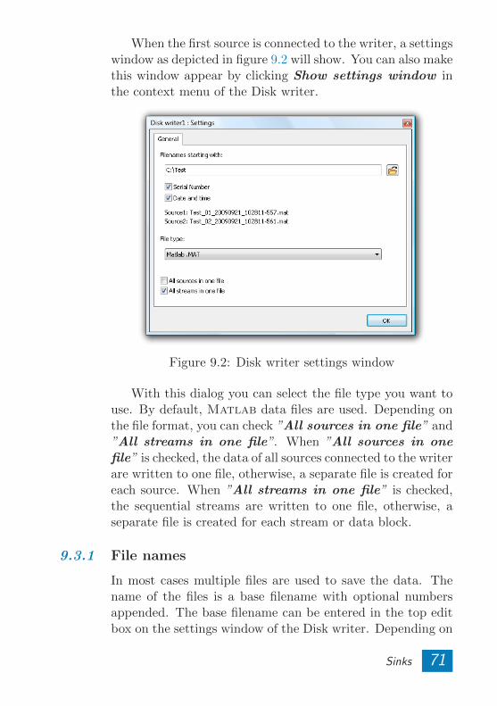
When the first source is connected to the writer, a settingswindow as depicted in figure 9.2 will show. You can also makethis window appear by clicking Show settings window inthe context menu of the Disk writer.

Figure 9.2: Disk writer settings window

With this dialog you can select the file type you want touse. By default, Matlab data files are used. Depending onthe file format, you can check ”All sources in one file” and”All streams in one file”. When ”All sources in onefile” is checked, the data of all sources connected to the writerare written to one file, otherwise, a separate file is created foreach source. When ”All streams in one file” is checked,the sequential streams are written to one file, otherwise, aseparate file is created for each stream or data block.

9.3.1 File names

In most cases multiple files are used to save the data. Thename of the files is a base filename with optional numbersappended. The base filename can be entered in the top editbox on the settings window of the Disk writer. Depending on

Sinks 71

the ”All sources in one file” and ”All streams in onefile” options, serial numbers will be appended to the basefilename.

The date and time in millisecond precision can also be in-cluded in the file names, to make sure they are always unique.An example of the resulting filename(s) is shown below theedit box. With a base filename D:\Test, the filenames willlook like this:

D:\Test XX YYY.mat,where XX and YYY are numbers. When ”All sources inone file” is off, the source number XX starting from 1 isused. When ”All streams in one file” is off, the streamnumber YYY starting from 0 is used.

When the option ”All streams in one file” is on, butfor some reason a new file is started, another number is ap-pended to the base filename. The filename will then look likethis:

D:\TestA XX.mat, where A is the file number, startingfrom 1. A new file may be started for different reasons:

• the previous file has reached the file size limit and wasclosed

• the user has clicked ”Close file(s)” in the menu of theDisk writer

When ”Date and time” is checked, the date and timewill be added to the file name in the following format:

YYYYMMDD HHMMSS-MMM

9.3.2 Limiting file size

By default the maximum file size is limited to 4 GiB. Becausemost current applications have problems handling such bigfiles, the Disk writer has an option to limit the file size to anarbitrary number of bytes. You can set a file size limit bychoosing Limit file size to in the menu if the Disk writer.

72 Chapter 9

On FAT32 file systems, the maximum allowed file size is4 GiB. On NTFS file systems, the files may be as big as thedisk.

9.3.3 Skipping data

By default all measurements are written to disk. It is alsopossible to change this behavior, such that one of every Nmeasurements is written.

This can for example be used to write the average of sev-eral measurements to disk. To do so, create an Average I/O(see 8.10) and connect it to a Disk writer sink. Set the boththe Averaging count and the Disk writer ’s Store one of ev-ery... setting to the same number. Disable the Runningaverage setting of the Average I/O.

9.3.4 File type options

Some file types, like CSV, have extra options. When such afile type is selected, its options will be displayed on a separatetab in the settings window.

The file format options for storing data with the Diskwriter are the same as for exporting data, described in chap-ter 10.4.

9.4 I2C Analyzer

Use the I2C analyzer to inspect an I2C bus. Just measurethe Clock and Data lines of the I2C bus with a scope andconnect the measuring channels to an analyzer sink. Thesink uses a window for its output. The output can be savedto a text file. In figure 9.3 you can see an example of theoutput of the analyzer.

The I2C analyzer needs two sources: the first connectedsource will be used as I2C SCL (clock) and the second con-nected source will be used as I2C SDA (data).

Sinks 73

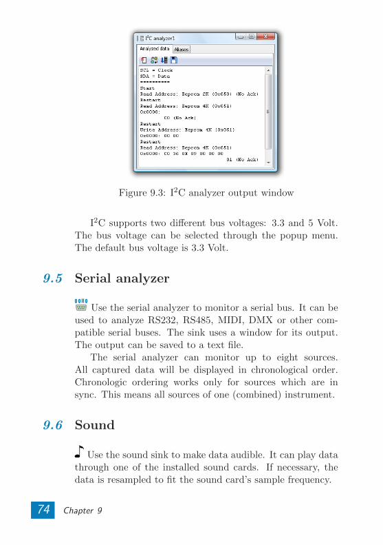
Figure 9.3: I2C analyzer output window

I2C supports two different bus voltages: 3.3 and 5 Volt.The bus voltage can be selected through the popup menu.The default bus voltage is 3.3 Volt.

9.5 Serial analyzer

Use the serial analyzer to monitor a serial bus. It can beused to analyze RS232, RS485, MIDI, DMX or other com-patible serial buses. The sink uses a window for its output.The output can be saved to a text file.

The serial analyzer can monitor up to eight sources.All captured data will be displayed in chronological order.Chronologic ordering works only for sources which are insync. This means all sources of one (combined) instrument.

9.6 Sound

Use the sound sink to make data audible. It can play datathrough one of the installed sound cards. If necessary, thedata is resampled to fit the sound card’s sample frequency.

74 Chapter 9

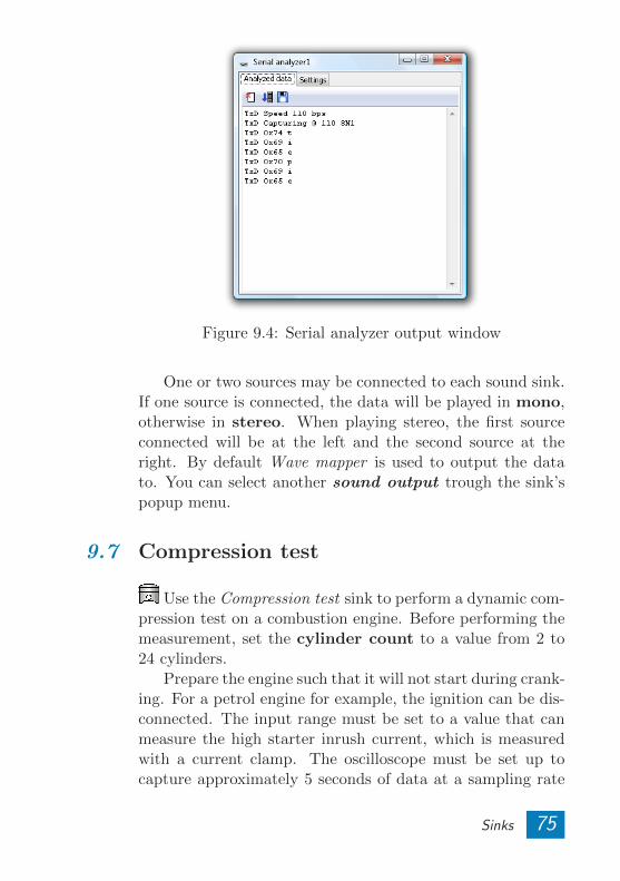
Figure 9.4: Serial analyzer output window

One or two sources may be connected to each sound sink.If one source is connected, the data will be played in mono,otherwise in stereo. When playing stereo, the first sourceconnected will be at the left and the second source at theright. By default Wave mapper is used to output the datato. You can select another sound output trough the sink’spopup menu.

9.7 Compression test

Use the Compression test sink to perform a dynamic com-pression test on a combustion engine. Before performing themeasurement, set the cylinder count to a value from 2 to24 cylinders.

Prepare the engine such that it will not start during crank-ing. For a petrol engine for example, the ignition can be dis-connected. The input range must be set to a value that canmeasure the high starter inrush current, which is measuredwith a current clamp. The oscilloscope must be set up tocapture approximately 5 seconds of data at a sampling rate

Sinks 75

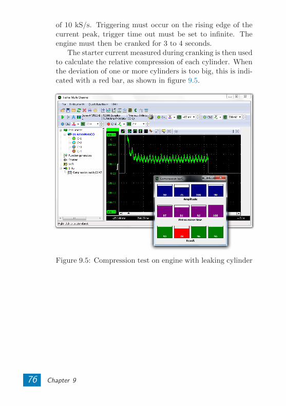
of 10 kS/s. Triggering must occur on the rising edge of thecurrent peak, trigger time out must be set to infinite. Theengine must then be cranked for 3 to 4 seconds.

The starter current measured during cranking is then usedto calculate the relative compression of each cylinder. Whenthe deviation of one or more cylinders is too big, this is indi-cated with a red bar, as shown in figure 9.5.

Figure 9.5: Compression test on engine with leaking cylinder

76 Chapter 9

Files 10The Multi Channel software uses various file types to loadand store data and settings. This chapter describes how youcan use these files.

10.1 File types

This section gives a short description of the TiePie file typesused in the Multi Channel software. Refer to section 10.4for information about other file types to which data can beexported.

10.1.1 Multi Channel TPS files

TiePie Settings (TPS) files, also known as setfiles, can beused to store all kinds of settings as well as data. The files cancontain instrument settings, graph settings, function genera-tor settings, etc. They can be used to save a (complicated)measurement setup for later use. The files can also containmeasured data, making it possible to examine the measureddata at a different location or at a later time.

There are three kinds of TPS files which can all includedata:

TPS type Contains

Desktop all settings of the instruments, func-tion generators, objects, graphs, etc.

Instrument settings of one instrumentFunction Generator settings of one function generator

When selecting a TPS file in the open dialog, you can seeits type in the tree view at the right side of the dialog. Theroot node in the tree view displays the file type.

Files 77

Desktop TPS files can be loaded as a whole, but you canalso load just parts from a file. See section 10.3 about loadingfiles for details.

10.1.2 Multi Channel TPO files

TiePie Objects (TPO) files can be used to store one or moreobjects with or without their data. The objects can be sour-ces, I/Os and sinks. When multiple objects are stored in aTPO file, the connections between these objects are stored aswell. This makes it possible to save e.g. a mathematical op-eration using multiple objects to a file for later use or to loadit multiple times if you want to perform the same operationon multiple sources.

The file structure of TPO files is very similar to that ofTPS files. The objects contained in TPO files can also befound in TPS files and can be loaded from both file types thesame way. See the sections about loading and saving objectsfor details.

10.1.3 WinSoft files

For backward compatibility, the Multi Channel software canopen files created by the WinSoft measuring software. Bothsettings and data can be loaded. The following file types aresupported:

WinSoft type Description

DAT Binary or ASCII data file. Must be ac-companied by a .GEG settings file.

SET WinSoft settings. Can contain instru-ment and function generator settings.

When a WinSoft file is opened via the file menu ordragged and dropped onto the main form, the current setupis closed and replaced by the setup in the file. When a Win-Soft file is opened via the popup menu of an instrument

78 Chapter 10

or function generator, the settings of that device are loaded,but the rest of the setup is left intact.

You can also open a WinSoft DAT file by clicking the loadbutton on the function generator control window.

10.2 Saving Files

The Multi Channel software can save to TPS and TPO files.As described in the types section, both file types are verysimilar. Refer to section 10.4 for information about other filetypes to which data can be exported.

10.2.1 Saving to a TPS file

As mentioned earlier, there are different kinds of TPS files.To save your complete setup in a Desktop type of file, createa TPS file with the Save as... item in the File menu. Tosave instrument settings and optionally data to an Instru-ment type of file, right-click the instrument in the objecttree and click Save as.... To save function generator settingsand optionally data to a Function Generator type of file,right-click the function generator in the object tree and clickSave as... or use the save button on the function generatorcontrol window.

10.2.2 Saving objects to a TPO file

In the object tree one or more sources, I/Os and sinks can beselected. You can save the selected object(s) to a TPO fileby right-clicking on the selection and choosing Save as...from the popup menu. The objects will be saved with allconnections they have in common.

Saving groups of objects can be handy when you wantto use the group with the same settings in another setup, orjust want to quickly create multiple equal groups of objectsto perform the same kind of processing on several sources.

Files 79

Figure 10.1: Saving two objects

After saving the file, you can open it multiple times to addthe objects in the file to the setup.

You can enter a description and choose to only store set-tings and no data by checking the ”Don’t store data” check-box.

Figure 10.2: TPO Save as dialog.

80 Chapter 10

10.3 Loading Files

A TPS, TPO or WinSoft file can be loaded in several ways.

10.3.1 Loading a whole file

The common way to load a file is to use the Load... itemin the File menu. By default, the whole file is loaded whenyou press ”Open”. Dragging and dropping a file on the mainform of the application will also load the whole file.

10.3.2 Loading just a part of a file

The open dialog of the Multi Channel software is extendedwith a tree view. This tree view represents the contents ofTPS and TPO files. The parts of the file that can be opened,are highlighted in the tree.

Figure 10.3: File Open dialog.

In the displayed open dialog, the selected file is a Desktoptype TPS file, containing a complete setup. By default, theDesktop node in the tree is selected and the total file is loadedwhen you press ”Open”.

As you can see in figure 10.3, the instrument and func-tion generator are highlighted as well. They can be loadedseparately, leaving the rest of your setup intact. To load the

Files 81

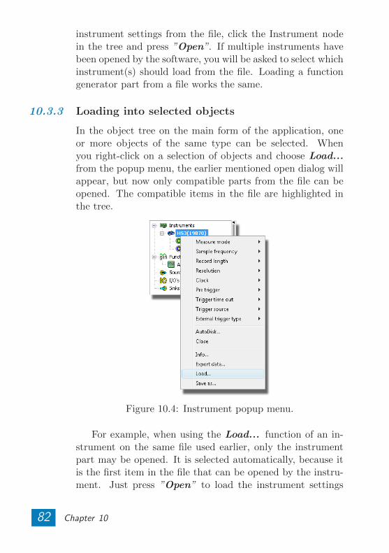
instrument settings from the file, click the Instrument nodein the tree and press ”Open”. If multiple instruments havebeen opened by the software, you will be asked to select whichinstrument(s) should load from the file. Loading a functiongenerator part from a file works the same.

10.3.3 Loading into selected objects

In the object tree on the main form of the application, oneor more objects of the same type can be selected. Whenyou right-click on a selection of objects and choose Load...from the popup menu, the earlier mentioned open dialog willappear, but now only compatible parts from the file can beopened. The compatible items in the file are highlighted inthe tree.

Figure 10.4: Instrument popup menu.

For example, when using the Load... function of an in-strument on the same file used earlier, only the instrumentpart may be opened. It is selected automatically, because itis the first item in the file that can be opened by the instru-ment. Just press ”Open” to load the instrument settings

82 Chapter 10

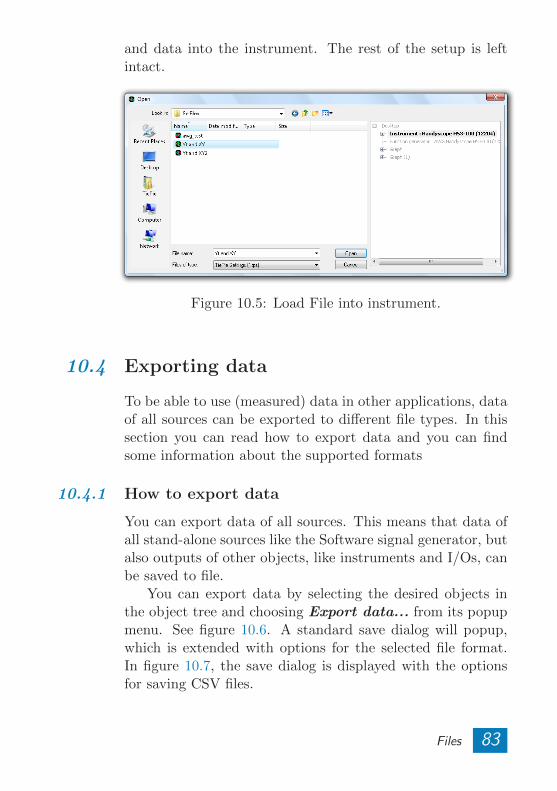
and data into the instrument. The rest of the setup is leftintact.

Figure 10.5: Load File into instrument.

10.4 Exporting data

To be able to use (measured) data in other applications, dataof all sources can be exported to different file types. In thissection you can read how to export data and you can findsome information about the supported formats

10.4.1 How to export data

You can export data of all sources. This means that data ofall stand-alone sources like the Software signal generator, butalso outputs of other objects, like instruments and I/Os, canbe saved to file.

You can export data by selecting the desired objects inthe object tree and choosing Export data... from its popupmenu. See figure 10.6. A standard save dialog will popup,which is extended with options for the selected file format.In figure 10.7, the save dialog is displayed with the optionsfor saving CSV files.

Files 83

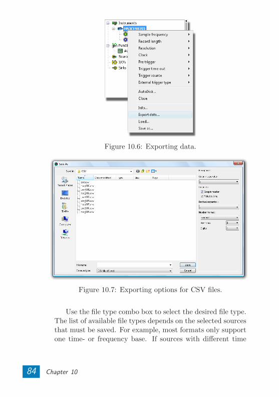
Figure 10.6: Exporting data.

Figure 10.7: Exporting options for CSV files.

Use the file type combo box to select the desired file type.The list of available file types depends on the selected sourcesthat must be saved. For example, most formats only supportone time- or frequency base. If sources with different time

84 Chapter 10

bases are selected, these formats will not appear in the filetype list.

10.4.2 Supported file types

At the time of writing is is possible to export data to thefollowing file formats:

• Binary (raw) (.bin)

• Comma Separated Values ASCII (.csv)

• Matlab (.mat) data (version 6)

• Wave audio (.wav)

It is possible that more file formats are supported in yourversion of the software. Refer to the online help file thatcomes with the software for a complete list of the file formatsand a description of their options.

Files 85

86 Chapter 10

Standard measurements AIn the cursor window of each graph and in meter objects,different measurements can be selected. These measurementsinclude:

• Maximum

• Minimum

• Top-Bottom

• Root Mean Square (RMS)

• Mean

• Variance

• Standard Deviation

• Frequency

• Duty cycle

• Duty cycle inverted

• Total Harmonic Distortion (THD)

• Crest factor

• Rise time

• Fall time

• dBm

The measurements are calculated over a sample range.When using the cursor window, the sample range is equal tothe samples in between the left and right cursor. In a meterobject, the sample range is equal to the post samples.

In the cursor window the following additional measure-ments are possible:

• Left

• Right

• Right-Left

• Slope

Standard measurements 87

A.1 Short description of the measurements

This section gives a short description of the standard mea-surements. Most measurements are very straight forward,but are explained for clarity. Some measurements are ex-plained with a formula. In these formulas m corresponds tothe index of the first sample in the sample range and n is thelast index. N is the number of samples in the sample rangeand is equal to n - m + 1. The ith sample is denoted as xi.

Maximum The measurement maximum is the highestvalue in the sample range.

Minimum The measurement minimum is the lowestvalue in the sample range.

Top-Bottom The measurement top-bottom, alsoknown as peak-peak is the highest value in the sample rangeminus the lowest value.

Root Mean Square (RMS) The measurement RMSis equal to the square root of the mean of the square of allsamples in the sample range. This is a whole mouth full anda formula is clearer:

RMS =

√√√√ 1

N

n∑i=m

x2i

Mean The measurement mean is the mean value of allsamples in the sample range.

Mean = x =1

N

n∑i=m

xi

88 Appendix A

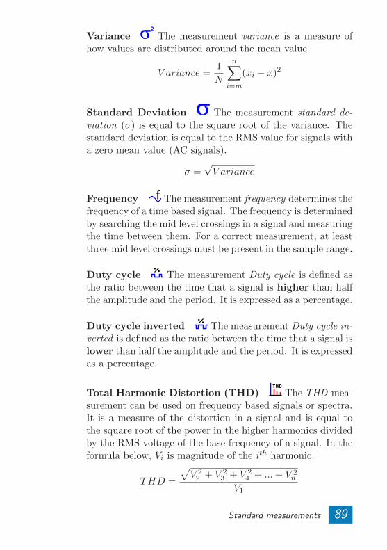
Variance The measurement variance is a measure ofhow values are distributed around the mean value.

V ariance =1

N

n∑i=m

(xi − x)2

Standard Deviation The measurement standard de-viation (σ) is equal to the square root of the variance. Thestandard deviation is equal to the RMS value for signals witha zero mean value (AC signals).

σ =√V ariance

Frequency The measurement frequency determines thefrequency of a time based signal. The frequency is determinedby searching the mid level crossings in a signal and measuringthe time between them. For a correct measurement, at leastthree mid level crossings must be present in the sample range.

Duty cycle The measurement Duty cycle is defined asthe ratio between the time that a signal is higher than halfthe amplitude and the period. It is expressed as a percentage.

Duty cycle inverted The measurement Duty cycle in-verted is defined as the ratio between the time that a signal islower than half the amplitude and the period. It is expressedas a percentage.

Total Harmonic Distortion (THD) The THD mea-surement can be used on frequency based signals or spectra.It is a measure of the distortion in a signal and is equal tothe square root of the power in the higher harmonics dividedby the RMS voltage of the base frequency of a signal. In theformula below, Vi is magnitude of the ith harmonic.

THD =

√V 22 + V 2

3 + V 24 + ...+ V 2

n

V1

Standard measurements 89

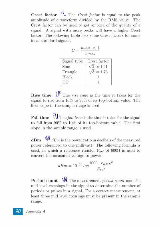
Crest factor The Crest factor is equal to the peakamplitude of a waveform divided by the RMS value. TheCrest factor can be used to get an idea of the quality of asignal. A signal with more peaks will have a higher Crestfactor. The following table lists some Crest factors for someideal standard signals.

C =max(| x |)xRMS

Signal type Crest factor

Sine√

2 ≈ 1.41

Triangle√

3 ≈ 1.73Block 1DC 1

Rise time The rise time is the time it takes for thesignal to rise from 10% to 90% of its top-bottom value. Thefirst slope in the sample range is used.

Fall time The fall time is the time it takes for the signalto fall from 90% to 10% of its top-bottom value. The firstslope in the sample range is used.

dBm dBm is the power ratio in decibels of the measuredpower referenced to one milliwatt. The following formula isused, in which a reference resistor Rref of 600Ω is used toconvert the measured voltage to power.

dBm = 10 ·10 log1000 · xRMS2

Rref

Period count The measurement period count uses themid level crossings in the signal to determine the number ofperiods or pulses in a signal. For a correct measurement, atleast three mid level crossings must be present in the samplerange.

90 Appendix A

Left The measurement left can be used in the cursorwindow. It is the value of the signal at the position of theleft cursor.

Right The measurement right can be used in the cursorwindow. It is the magnitude of the signal at the position ofthe right side cursor.

Right-Left The measurement right-left can be used inthe cursor window. It is the difference between the magnitudeof the signal at the position of the right and left cursor.

Slope The slope of a signal is the change of magnitudedivided by the elapsed time. The measurement slope deter-mines the slope in a signal between the left and the rightcursor.

Slope =xright − xlefttright − tleft

Standard measurements 91

92 Appendix A

Hotkeys BFor the most frequently used functions, hotkeys have been in-cluded to allow faster and easier control of the Multi Channelsoftware.

Common:

F1 Context sensitive helpSHIFT + (1 . . . 0) Select graph 1 through 10CTRL + (1 . . . 0) Select instrument 1 through 10

ALT + S Search instruments

Per instrument:

F3 / F4 Decrease / increase sample frequencyF11 / F12 Decrease / increase record length

S Start / StopO Start Oneshot / Stop0 Trigger timeout = 01 Trigger timeout = 1 sec.

W Trigger timeout = infiniteSHIFT + ← / → Change pre-/post samples ratio

<space> Directly force a triggerQ Perform a quick auto setup

CTRL + Q Perform a quick auto setup andkeep following the signal

Hotkeys 93

Per channel:

F5 / F6 Decrease / increase rangeR Autoranging on / off

F7 / F8 Trigger level[ / ] Trigger hysteresis

A AC-couplingD DC-coupling

The mentioned channel hotkeys by default apply to chan-nel 1. If the hotkeys are used with the keys mentioned in tableB.1, the hotkey applies to the indicated channel, of the activeinstrument.

Channel Key(s)

Ch. 1 –Ch. 2 CTRLCh. 3 SHIFTCh. 4 CTRL + SHIFTCh. 5 ALTCh. 6 ALT + CTRLCh. 7 ALT + SHIFTCh. 8 ALT + CTRL + SHIFT

Table B.1: Selecting channel for hotkeys

94 Appendix B

Per graph:

L InterpolationU Zoom out

CTRL + DEL Clear graphSHIFT + DEL Delete graph

← / → Move scroll bar sliderCTRL + ← / → Move left edge of the scroll bar slider

↑ / ↓ Move right edge of the scroll bar sliderT Full record viewX XY-modeY Yt-mode

Per AWG:

F Enter the frequencyA Enter the amplitudeO Enter the offsetS Enter the symmetryP Enter the phaseB Enter the burst countD Enter the sweep duration

Hotkeys 95

96 Appendix B

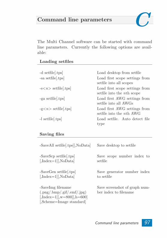
Command line parameters CThe Multi Channel software can be started with commandline parameters. Currently the following options are avail-able:

Loading setfiles

-d setfile[.tps] Load desktop from setfile

-sa setfile[.tps] Load first scope settings fromsetfile into all scopes

-s<n> setfile[.tps] Load first scope settings fromsetfile into the nth scope

-ga setfile[.tps] Load first AWG settings fromsetfile into all AWGs

-g<n> setfile[.tps] Load first AWG settings fromsetfile into the nth AWG

-l setfile[.tps] Load setfile. Auto detect filetype

Saving files

-SaveAll setfile[.tps][,NoData] Save desktop to setfile

-SaveScp setfile[.tps][,Index=1][,NoData]

Save scope number index tosetfile

-SaveGen setfile[.tps][,Index=1][,NoData]

Save generator number indexto setfile

-SaveImg filename(.png/.bmp/.gif/.emf/.jpg)[,Index=1][,w=800][,h=600][,Scheme=Image standard]

Save screenshot of graph num-ber index to filename

Command line parameters 97

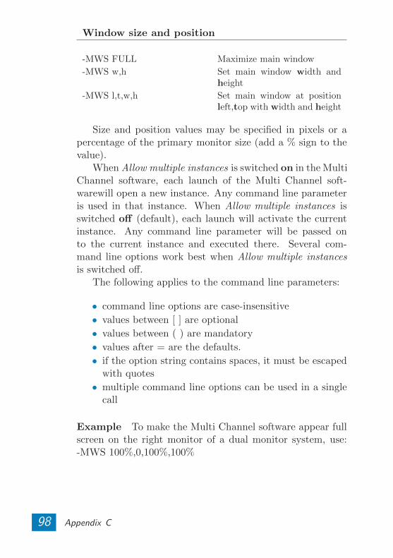
Window size and position

-MWS FULL Maximize main window

-MWS w,h Set main window width andheight

-MWS l,t,w,h Set main window at positionleft,top with width and height

Size and position values may be specified in pixels or apercentage of the primary monitor size (add a % sign to thevalue).

When Allow multiple instances is switched on in the MultiChannel software, each launch of the Multi Channel soft-warewill open a new instance. Any command line parameteris used in that instance. When Allow multiple instances isswitched off (default), each launch will activate the currentinstance. Any command line parameter will be passed onto the current instance and executed there. Several com-mand line options work best when Allow multiple instancesis switched off.

The following applies to the command line parameters:

• command line options are case-insensitive

• values between [ ] are optional

• values between ( ) are mandatory

• values after = are the defaults.

• if the option string contains spaces, it must be escapedwith quotes

• multiple command line options can be used in a singlecall

Example To make the Multi Channel software appear fullscreen on the right monitor of a dual monitor system, use:-MWS 100%,0,100%,100%

98 Appendix C

Index

ABS, 59AC coupling, 31Active instrument, 6, 28Add, 58Alias, 51Analyzer

I2C, 12, 73CAN, 12, 67Serial, 12, 74

Arbitrary data, 44ASCII files, 70, 85Auto disk, 33Auto-ranging, 32Average, 61AWG, 37Axis, 21

Basic measurements, 7Binary files, 70, 85

CAN analyzer, 12, 67Channel bar, 27Combining instruments, 35Compression test, 75Connecting objects, 49Coupling, 31Creating objects, 49Crest factor, 90CSV files, 70, 85Cursors, 19

Data collector, 10, 63dBm, 90DC coupling, 31Differentiate, 59Disconnecting objects, 50Disk writer, 70Displaying data, 15Duty cycle, 64, 89

Duty cycle inverted, 89

Exporting data, 83

Fall time, 90FFT, 10, 64File

ASCII, 70, 85Binary, 70, 85CSV, 70, 85HTML, 70Loading, 81Matlab, 70, 85Rich Text Format, 70Saving, 79Setfile, 77Text, 70TPO, 78TPS, 77Wave audio, 70, 85WinSoft, 78

Frequency, 89

Gain/Offset, 57Graph, 15Graph mode, 16Graph scheme, 14Grid, 69

HTML files, 70

I2C analyzer, 12, 73Input range, 32Instrument bar, 26Integrate, 60Interpolation, 18Invert, 57

J1939 decoder, 68

99

Language, 13Limiter, 62Log, 60Low-pass filter, 61

Math, 52, 58Matlab files, 70, 85Maximum, 88Mean, 88Measure mode, 28

Stream, 10, 33Meter, 23, 69Meter scheme, 14Min/Max detector, 61Minimum, 88Multiply/Divide, 58

ObjectChanging settings, 49Connecting, 49Creating, 49Disonnecting, 50types, 48

Object tree, 48Oscilloscope in XY mode, 8Oscilloscope in Yt mode, 8

Peak-peak, 88Period count, 90Post-samples, 30Pre-samples, 30Pre-trigger, 30Printing, 13Pulse decoder, 66

Quick functions, 7

Range, 32Record length, 29Reference, 18Resampler, 62Resolution, 29Rise time, 90

RMS, 88RPM-detector, 65

Sample frequency, 29Scale, 21Sensors, 57Serial analyzer, 12, 74Setfile, 77Settings, 13Slope, 91SoftGen, 55Source, 55Spectral leakage, 64Spectrum analyzer, 9, 64Sqrt, 58Standard Deviation, 89Start measuring, 27Streaming mode, 10, 33Sum, 52, 58

Table, 69Text files, 70THD, 89Top-Bottom, 88Transient recorder, 10Trigger

Hysteresis, 32Level, 32Source, 30Time-out, 30Type, 32

UnitChanging, 55

Variance, 89Voltmeter, 11, 23, 69

Wave audio files, 70, 85

XY mode, 16

Yt mode, 16

100

If you have any suggestions and/or remarks regarding this manual,please contact:

TiePie engineeringKoperslagersstraaat 378601 WL SNEEKThe Netherlands

Tel.: +31 515 415 416Fax: +31 515 418 819E-mail: support@tiepie.nlSite: www.tiepie.com