Embed Size (px)
Citation preview
Multi-Carrier CDMA in an Indoor WirelessRadio Channel
Nathan Yee and Jean-Paul Linnartz
University of California at BerkeleyBerkeley, California 94720
Multi-Carrier CDMA
This report summarizes the research findings of the MICRO project 93-101, entitled "Frequency - Code Division Mul-
tiple Access: a New Spreading Technique for Radio Communications over Multipath Channels", supported by Teknekron
Communication Systems, Berkeley and the California MICRO Program. Principal Investigator is Professor J.P. Linnartz,
Industrial Liaison is Dr. G. Fettweis.
Multi-Carrier CDMA
Table of Contents
CHAPTER 1 Introduction 11.1 Introduction 1
CHAPTER 2 Multipath Channels 32.1 Multipath Channels 3
CHAPTER 3 Principles of MC-CDMA 63.1 What is MC-CDMA? 6
3.2 The F-parameter 7
3.3 Comparison with Conventional Modulation Techniques 8
3.4 The Indoor Environment and MC-CDMA 10
3.5 The Codes 11
3.6 Transmitter Model 11
3.7 Channel Model 13
3.8 Receiver Model 14
3.9 Equalization 16
CHAPTER 4 Analysis of the Performance of MC-CDMA in Rayleigh andRician Fading Channels 20
4.1 Rayleigh Fading 20
4.2 Rician Fading 28
CHAPTER 5 Numerical Results 335.1 Rayleigh Fading 33
5.2 Rician Fading 38
CHAPTER 6 Conclusion 44
Appendix A Statistical Properties of the Noise46
Appendix B Statistical Properties of the Interference 49
Appendix C Simplification of CLT Expressions 52
References 53
Multi-Carrier CDMA 1
CHAPTER 1 Introduction
1.1 Introduction
With a surging increase in demand for personal wireless radio communications within the past decade, there is a grow-
ing need for technological innovations to satisfy these demands. Future technology must be able to allow users to effi-
ciently share common resources, whether it involves the frequency spectrum, computing facilities, databases, or storage
facilities. As with mobile cellular telephony, the driving forces behind this demand includes the mobility and flexibility
that this technology provides. In contrast to wired communications, future personal communication networks will allow
users the connection to a multitude of resources while enjoying the freedom of mobility. A particular area of growing
interest is indoor wireless communications.
In an indoor environment, the use of a wireless communication link removes any need for wiring. Besides the
removal of the costs associated with wiring, wireless links allow the network to operate undisturbed while new users are
added.
While there is a strong desire for this technology, there are many obstacles and issues that need to be addressed. The
issue of portability places constraints on the size and on the power consumption of the terminals. In addition, transmis-
sions in an indoor environment face the harsh degradations of multipath channels.
In this document, a novel digital modulation and multiple access scheme called Multi-Carrier CDMA (MC-
CDMA) [1] [2] [3] is analyzed. Although this modulation technique in this report is applied primarily to an indoor wire-

Introduction
2 Multi-Carrier CDMA
less radio network, this transmission scheme may have other applications. One possible application is vehicle-to-vehicle
communications for Intelligent Highway Vehicle Systems (IHVS). The deciding factors on whether this technique is fea-
sible for a certain application depends largely on the physical channel and the baud rates of interest. Under appropriate
conditions, MC-CDMA signals will propagate through multipath channels with little distortion1.
Although MC-CDMA resembles the signal structure for OFDM when the subcarriers are spaced as closely as possible,
the manner in which the subcarriers are utilized is very different. In [4] [5], OFDM is discussed as a means of decreasing
the effective baud rate by transmitting different data symbols on different subcarriers. With MC-CDMA, the same data bit
is transmitted over all subcarriers without changing the original baud rate.
In [3], a bound on the bit error rate for convolutionally-coded MC-CDMA is presented. In this scheme, a maximum-
likelihood detection is performed on the received signal where all signals including the interference are considered in the
decision making process. For the MC-CDMA system that we are analyzing, the receiver is assumed to be of a much sim-
pler form, detecting only for the desired signal using classical diversity theory.
The general organization of this document is as follows. The discussion begins with the review of multipath channels
and its implications on wireless communications. In Chapter 3, MC-CDMA is described in detail. It is compared to other
conventional modulation techniques; differences and similarities are pointed out. In the process, motivations for this new
technique are discussed. Next, implementation of this modulation scheme will be discussed with a possible transmitter
and receiver model. In the receiver model, different frequency equalization techniques are considered. In Chapter 4, the
performance of this technique in an indoor wireless environment is evaluated for Rayleigh and Rician fading channels.
Numerical results are presented and discussed in Chapter 5.
1. In this report, "distortion" means linear distortion or dispersion.
Multipath Channels
Multi-Carrier CDMA 3
CHAPTER 2 Multipath Channels
2.1 Multipath Channels
When a binary phase-shift keying (BPSK) modulated signal is transmitted over a wireless channel, the transmitted sig-
nal decomposes into multiple copies of the original signal corresponding to multiple path reflections off of the surround-
ing environment. Each path will experience an attenuation, a phase delay and a time delay. At the receiver, the received
signal consists of the superposition of these paths. Because of the random nature of the channel effects mentioned above,
the paths may add destructively. This phenomenon creates an obstacle for wireless communications.
Two parameters that are often used to characterize multipath channels are the delay spread and the coherence
bandwidth[6]. Thedelay spread,Td, is a measure of the length of the impulse response of the channel. Delay spreads lead
to intersymbol interference (ISI) and consequently degrade the performance of the system and complicate the receiver
design. In indoor environments, the root mean square (r.m.s) delay spread is in general small with typical values in the
range of 10 - 50 ns.[7]. Also of interest is the number of resolvable paths, which is defined to be
(1)
whereTd is the maximum delay spread andTb is the symbol duration. For narrowband communications, there is usually
only one resolvable path for transmission rates up to 1 Mbauds/sec.
As a measure of the correlation of the fading between frequencies, the coherence bandwidth is directly related to the
delay spread. For an exponentially distributed delay spread power profile, the coherence bandwidth is given as
. (2)
Two frequencies lying within the coherence bandwidth are likely to experience correlated fading.
LTm
Tb
1+=
BWc1
2πTd
=
Multipath Channels
4 Multi-Carrier CDMA
Another channel phenomenon associated with wireless communications is the Doppler spread. While it may be inter-
preted as a measure of the variation of the shift in the carrier frequency, it is in some ways more intuitive to view it as a
measure of the rate at which the channel changes. Small doppler spreads imply a large coherence time or a slowly chang-
ing channel. Measurements indicate that Doppler shifts are relatively small and typically in the range of 0.3 to 6.1 Hz[8]
in the indoor environment. Thus, the channel may be assumed to be constant over the symbol duration,Tb, for baud rates
up to 1 Mbaud/sec.
Within a small time window in which the effects of the channel are relatively constant, the received signal consists of
the contribution from the paths that arrive within this interval. Each path may be treated as a vector with an amplitude and
phase. If the terminal is moving or the surrounding environment is changing, the effects of the channel will randomly
change with time. Thus, at some points in time, the paths may add destructively and in others constructively. Obviously,
the case that is undesirable is when the channel attenuates the signal. Two distributions that are commonly used to
describe the random amplitudes resulting from multipath channels are the Rayleigh and Rician distributions.
If there is no line-of-sight (LOS) component in the received signal, i.e, when the direct path is obstructed as with prop-
agation in an outdoor environment over long distances, the received signal consists only of scattered components due to
reflections with no dominant path. The received signal can be separated into an in-phase and a quadrature component
where each path will contribute an in-phase and a quadrature component. Assuming that there are a very large number of
paths, the in-phase and quadrature components can be assumed to be zero-mean Gaussian random variables by the Central
Limit Theorem (CLT). Thus, the overall amplitude of the signal that results from the vector addition of all components is
by definition Rayleigh distributed and the phase is uniformly distributed on the interval of [0,].
The Rayleigh distribution of is defined to be
(3)
where is the variance of the in-phase and quadrature components. Two statistical quantities of interest are the mean
and the second moment of the Rayleigh random variable. They can be determined to be
. (4)
If there is a direct LOS component, as in the case of indoor environments, the received signal will most likely consis-
tent of a dominant component corresponding to the LOS path and a scattered component due to reflections. Arbitrarily
2π
ρ
fρ ρ( )ρ
σ2e
ρ2
2σ2 −
=
σ2
Eρπ2
σ= Eρ2 2σ2=
Multipath Channels
Multi-Carrier CDMA 5
orienting the in-phase and quadrature components so that the LOS component is in-phase, the received signal amplitude,
, has a Rician distribution given by
(5)
where represents the power of the scattered in-phase and quadrature components, is the amplitude of the LOS
component and is the zeroth order modified Bessel function. The Rician distribution is often characterized by the
RicianK-factor, which is defined to be the ratio of the power of the LOS component to the power of the scattered compo-
nent and is given as
. (6)
Measurements of the indoor environments indicate that a RicianK-factor of 10 is a typical value for an open-office inte-
rior floor plan[9] [10]. A statistical quantity that is of interest is the mean of the Rician distribution which can be found to
be
(7)
where represents the first order modified Bessel function.
Many studies have been done on the channel modelling of indoor environments. The statistical models given
in [11] [12] may be more appropriate for wideband signals where there are many resolvable paths rather than in narrow-
band communications where there is usually one resolvable path (i.e., ).
ρ
fρ ρ( )ρ
σ2e
ρ2 b02+
2σ2−
I0
b0ρ
σ2 =
σ2 b0
I0 ρ( )
Kb0
2
2σ2=
Eρ e K 2⁄− π2 K 1+( )
p 1 K+( ) I0K2
( ) KI1K2
( )+=
I1 K( )
Td Tb«

Principles of MC-CDMA
6 Multi-Carrier CDMA
CHAPTER 3 Principles of MC-CDMA
3.1 What is MC-CDMA?
Multi-carrier CDMA is a digital modulation technique where a single data symbol is transmitted at multiple narrow-
band subcarriers with each subcarrier encoded with a phase offset of 0 or based on a spreading code. The narrowband
subcarriers are generated using BPSK modulated signals, each at different frequencies which at baseband are at multiples
of a harmonic frequency, . Consequently, the subcarriers are orthogonal to each other at baseband, and the compo-
nent at each subcarrier may be filtered out by modulating the received signal with the frequency corresponding to the par-
ticular subcarrier of interest and integrating over a symbol duration. The orthogonality between subcarrier frequencies is
maintained if the subcarrier frequencies are spaced apart by multiples of where is an integer. Throughout this
document, F, which will be used to describe the spacing between subcarrier frequencies for an MC-CDMA signal, will be
referred to as the F-parameter. An example of an MC-CDMA signal in the frequency domain for F = 6 is shown in Fig.
1c.
The phase at each subcarrier corresponds to one element of the spreading code. For a spreading code of length N,
there are N subcarriers. Throughout this paper, N will be referred to as the spreading factor. This modulation scheme is
also a multiple access technique in the sense that different users will use the same set of subcarriers but with a different
spreading code that is orthogonal to the code of all other users. Thus, it is important to point out that there exist two levels
of orthogonality. While the subcarriers frequencies are orthogonal to each other, and the spreading codes are also orthog-
onal to each other.
Upon careful examination, the discrete-time version of the signal can be viewed as the Discrete Fourier Transform
(DFT) of a Direct Sequence - Code Division Multiple Access (DS-CDMA) signal, i.e., the signal is CDMA-coded in fre-
π
1 Tb⁄
F Tb⁄ F

The F-parameter
Multi-Carrier CDMA 7
quency. This scheme can also be considered as a spread spectrum technique since the signal is spread over a larger band-
width than necessary in order to achieve frequency diversity.
3.2 The F-parameter
In order to obtain a compact signal in frequency, it would be desirable to space the subcarriers as closely together as
possible. The closest possible spacing between subcarriers is where F = 1. With this particular spacing, the struc-
ture of the signal is exactly that of Orthogonal Frequency Division Multiplexing (OFDM) [4] [5].
3.2.1 F = 1 and OFDM
Although OFDM and MC-CDMA have the same signal structure, they are very different in how the subcarriers are
actually used to transmit data. With OFDM, different data symbols are transmitted at different subcarriers. These sets of
data symbols can be encoded with error correction or detection codes to compensate for the loss of individual subcarriers
and their corresponding data symbols. The goal of OFDM is to reduce the effective transmission rate and consequently
increase the symbol duration. As a result, the OFDM signal is affected less by delay spreads and ISI because of the longer
symbol duration. In addition, if the channel changes rapidly, i.e., when there are large Doppler shifts, the longer symbol
duration helps to average out the signal over these fluctuations and occurrences of deep fades in time. The implementa-
tion of multiple access in OFDM is different from that of MC-CDMA in that different users do not use the same set of
subcarriers. Multiple access in OFDM may be implemented by having different users transmit on different sets of subcar-
riers (frequency division multiplexing) or to have different users contribute to a data set that will be assigned to the same
OFDM signal. Thus, as it can be seen, OFDM and MC-CDMA differ greatly in the utilization of the subcarriers.
Since MC-CDMA has the same signal structure for F = 1 as OFDM, some conclusions and results about OFDM can
be applied to MC-CDMA for F = 1. One conclusion is that MC-CDMA for F = 1 is spectrally efficient. Since the subcar-
riers are spaced closely together, an efficient bits/Hz ratio is obtained [5]. In addition, since the edges of the signal in fre-
quency are formed by narrowband sinc( ) functions, the drop off of the MC-CDMA (F = 1) signal spectrum at its edges is
very sharp. Consequently, the spectral leakage into adjacent frequency bands is small. Another conclusion that can be
drawn from the similarity with OFDM will be brought up when the implementation aspects of MC-CDMA are discussed.
1 Tb⁄

Principles of MC-CDMA
8 Multi-Carrier CDMA
3.2.2 F very Large
While one would desire a spectrally compact and efficient signal, there is also the conflicting goal of frequency diver-
sity. By transmitting the signal at multiple subcarriers, it is hoped that only a few of the subcarriers will be severely atten-
uated with the majority of the subcarriers passing through the channel with little distortion. The degree to which this goal
coincides with the physical channel depends on the coherence bandwidth, , of the channel. If several subcarriers lie
within the coherence bandwidth, then it is statistically likely that the loss of one subcarrier implies the loss of all the sub-
carriers within . In this case, frequency diversity is not achieved.
Consequently, depending on the actual physical channel, one may desire to space the subcarriers as far apart as possi-
ble, corresponding to a large F-parameter, in order to obtain frequency diversity. This implies that frequency diversity can
be achieved with a relatively small spreading factor with MC-CDMA using an appropriate value for . While this may
not make the MC-CDMA signal spectrally compact, a possible solution is to have other programs or applications (not
necessarily constructed of MC-CDMA signals) assigned to the gaps between the narrowband subcarriers.
3.3 Comparison with Conventional Modulation Techniques
In order to understand the motivations for MC-CDMA, it is helpful to compare it with other conventional modulation
techniques.
3.3.1 Narrowband (BPSK) signals
Narrowband communications [13] has the desirable quality of being relatively immune to intersymbol interference in
an indoor environment as the symbol duration is greater than the delay spread ( << ). However, this same condition
implies that the signal bandwidth is smaller than the coherence bandwidth. Consequently, a narrowband signal will expe-
rience the undesirable effect of experiencing flat fading. Depending on the location of the receiver, the entire signal may
be located in a deep fade that significantly attenuates the entire signal (see Fig. 1a).
3.3.2 Direct Sequence - Spread Spectrum Code Division Multiple Access
To combat the effect of flat fading, conventional DS-CDMA Spread Spectrum [14] [15] may be applied so that the sig-
nal bandwidth is spread over a bandwidth larger than the coherence bandwidth. A DS-CDMA signal is generated by mul-
BWc
BWc
F
Td Tb

Comparison with Conventional Modulation Techniques
Multi-Carrier CDMA 9
tiplying each user data symbol by a fast binary antipodal sequence where the chip duration is . These faster
variations in time increase the bandwidth of the signal. Consequently, if the spreading factor is sufficiently large, the sig-
nal experiences frequency-selective fading, and it is unlikely that the entire signal will be lost to fades in frequency (see
Fig 1b).
In the process of generating this signal, the resolution in time at the receiver is increased by a factor of N, and the sig-
nal is more susceptible to inter-chip interference. This inter-chip interference results in complexity in the design of the
receiver and synchronization issues that must address the increase in the number of resolvable paths. One method of
implementing the receiver is with a Rake receiver where the receiver consists of multiple branches of receivers, each syn-
chronized in time to a resolvable path. If is very small compared to , then the number of branches (resolvable
paths) in the Rake receiver will be prohibitively large.
Although the implementation of the Rake receiver is possible, there are complications and limitations that arise for
certain applications. With indoor wireless office communications, there is the issue of power consumption. The portable
terminals are designed under a low power consumption constraint. Measurements of the indoor wireless radio channel
a)
b)
c)
d)
Fig. 1 Spectrum of a) Narrowband signal, b) DS-CDMA signal, c) MC-CDMA signal before the channel, and d) MC-CDMA after the channel. The (---) represents the channel while the solid line represents the signal.
Tb N⁄
Tb N⁄ Td

Principles of MC-CDMA
10 Multi-Carrier CDMA
have shown that some bands of frequency, such as the deregulated ISM band, have a relatively flat channel and a large
coherence bandwidth. In order to achieve frequency diversity with a DS-CDMA system in such an environment, very
large spreading factors would be required. This large spreading factor translates to a prohibitively large power consump-
tion due to signal processing and synchronization. In addition, large spreading factors would imply the usage of a large
physical bandwidth and consequently a spectrally inefficient allocation of resources.
3.3.3 MC-CDMA
MC-CDMA addresses the issue of how to spread the signal bandwidth without increasing the adverse effect of the
delay spread. As a MC-CDMA signal is composed of N narrowband subcarrier signals each of which has a symbol dura-
tion much larger than the delay spread, a MC-CDMA signal will not experience an increase in susceptibility to delay
spreads and ISI as does DS-CDMA. In addition, since the F-parameter can be chosen to determine the spacing between
subcarrier frequencies, a smaller spreading factor than one required by DS-CDMA can be used to make it unlikely that all
of the subcarriers are located in a deep fade in frequency and consequently achieve frequency diversity (see Fig. 1c and d).
3.4 The Indoor Environment and MC-CDMA
In an indoor environment, the characteristics of the channel allow for an MC-CDMA signal to experience relatively
little distortion. As mentioned in the section on multipath channels, indoor wireless radio channels are typically charac-
terized by small delay spreads and small doppler shifts. As mentioned above, MC-CDMA signals are composed of nar-
rowband subcarrier signals with a symbol duration greater than the delay spread. Equivalently, the signal bandwidth is
smaller than the coherence bandwidth. Thus, the channel that each subcarrier experiences can be approximated as flat
fading which only attenuates the entire signal leaving the general shape of the signal undistorted. Thus, this reasoning
implies that the lengthening or dispersion of the signal in time is negligible. Small doppler shifts are desirable for MC-
CDMA signals since doppler shifts larger than or on the order of the bandwidth of the narrowband signals would make
the reception of these signals very difficult.

The Codes
Multi-Carrier CDMA 11
3.5 The Codes
Up until now, we have been very vague about the specific spreading codes that may be used. In this section, we will
discuss possible codes that may be used. The length of the codes are assumed to be equal to the number of subcarriers,N.
The individual elements of the code will be referred to as chips. Each chip of a code belongs to the set. The
property of the codes that is desired is for the codes of different users to be orthogonal, i.e.,
. (8)
One possible set of codes are the pseudo-random codes (pn-codes) generated by shift registers. These codes are called
pseudo-random because they appear to be random with a balanced run of -1’s and 1’s. Using a shift register of lengthn,
the length of the code that is generated is . Thus, only odd length codes can be generated. This observation implies
that the codes are not perfectly orthogonal since there is not a perfect balance between -1’s and 1’s. To be precise, the
inner product between any two different pn-codes is -1. In addition, if the transmitter is to be implemented with an FFT,
the code length should be a multiple of 2, which is not possible with pn-codes.
Another possible set of codes are the Walsh-Hadamard codes. These codes are generated by matrix operations. The
basic matrix unit of Walsh-Hadamard code generation is
. (9)
Walsh codes of length can be generated with the following recursive matrix operation
(10)
where the matrix, , of size is formed using the matrix, , of size with given inEq. (9).
Each row of the matrix, , gives the code for one user. It can be verified that these codes are perfectly orthogonal in the
sense that the inner product between any two different codes (rows of the matrix) is zero.
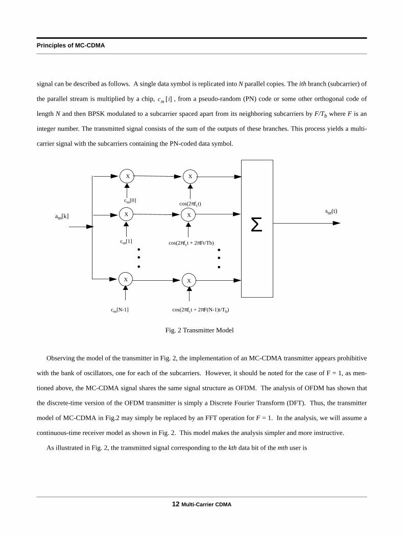
3.6 Transmitter model
Shown in Fig. 2 is a model of the transmitter for one possible implementation of an MC-CDMA system. The input
data symbols, am[k], are assumed to be binary antipodal wherek denotes thekth bit interval andm denotes themth user. In
the analysis, it is assumed thatam[k] takes on values of -1 and 1 with equal probability. The generation of an MC-CDMA
1 1−,{ }
cl i[ ] cm i[ ]i 0=
N 1−
∑ Nδl m,=
2n 1−
H01 11 1−
=
2n
Hn
Hn 1− Hn 1−
Hn 1− Hn 1−−=
Hn 2n 2n× Hn 1− 2n 1− 2n 1−× H0
Hn
Principles of MC-CDMA
12 Multi-Carrier CDMA
signal can be described as follows. A single data symbol is replicated into N parallel copies. The ith branch (subcarrier) of
the parallel stream is multiplied by a chip, , from a pseudo-random (PN) code or some other orthogonal code of
length N and then BPSK modulated to a subcarrier spaced apart from its neighboring subcarriers by F/Tb where F is an
integer number. The transmitted signal consists of the sum of the outputs of these branches. This process yields a multi-
carrier signal with the subcarriers containing the PN-coded data symbol.
Observing the model of the transmitter in Fig. 2, the implementation of an MC-CDMA transmitter appears prohibitive
with the bank of oscillators, one for each of the subcarriers. However, it should be noted for the case of F = 1, as men-
tioned above, the MC-CDMA signal shares the same signal structure as OFDM. The analysis of OFDM has shown that
the discrete-time version of the OFDM transmitter is simply a Discrete Fourier Transform (DFT). Thus, the transmitter
model of MC-CDMA in Fig.2 may simply be replaced by an FFT operation for F = 1. In the analysis, we will assume a
continuous-time receiver model as shown in Fig. 2. This model makes the analysis simpler and more instructive.
As illustrated in Fig. 2, the transmitted signal corresponding to the kth data bit of the mth user is
cm i[ ]
Fig. 2 Transmitter Model
X
cos(2πfct + 2πF(N-1)t/Tb)
X
cos(2πfct + 2πFt/Tb)
X
cos(2πfct)
X
cm[N-1]
X
cm[1]
X
cm[0]
am[k]
Σsm(t)
..
. ...

Channel Model
Multi-Carrier CDMA 13
(11)
where cm[0], cm[1], ... , cm[N-1] represents the spreading code of the mth user and is defined to be an unit amplitude
pulse that is non-zero in the interval of [0, Tb].
3.7 Channel Model
In Chapter 2, multipath channels were discussed and the common distribution functions encountered when character-
izing the random amplitude effects of the channel were described. A more detailed discussion of the channel model that is
appropriate for MC-CDMA systems in an indoor environment will follow.
In this document, we will focus on a frequency-selective channel with 1/Tb << BWc << F/Tb. For the symbol rates of
interest, this model implies that each modulated subcarrier with transmission bandwidth of 1/Tb does not experience sig-
nificant dispersion (Tb >> Td) and overlapping between adjacent data symbols (ISI). It is also assumed that the amplitude
and phase remain constant over a symbol duration, Tb, (i.e., Doppler shifts due to the motion of terminals and the sur-
rounding environment are negligible) which as mentioned earlier is a reasonable assumption. The condition BWc << F/Tb
implies that for different subcarriers the fading is assumed to be independent. For symbol rates on the order of 1 Mbauds/
sec, this assumption is reasonable since the symbol duration of secs is much larger that the typical r.m.s delay
spreads of 50 ns.
Assuming flat fading at the subcarriers, the effects of the channel for a signal subcarrier can be characterized by 2
parameters: an amplitude scaling and a phase distortion. The transfer function of the continuous-time fading channel
assumed for the mth user in the indoor environment can be represented as
(12)
where ρm,i and θm,i are the random amplitude and phase effects of the channel of the mth user at frequency fc+i(F/Tb). In
addition, as mentioned above, it is assumed that the and remain approximately constant over the symbol dura-
tion, Tb.
The local-mean power at the ith modulated subcarrier of the mth user is defined to be
(13)
sm t( ) cm i[ ] am k[ ] 2πfct 2πiFTb
t+( )cosi 0=
N 1−
∑= pTbt kTb−( )
cm i[ ] 1 1,−{ }∈
pTbt( )
1 10 6−×
Hm fc iFTb
+ ρm i, ejθm i,=
ρm i, θm i,
pm i, E ρm i, 2πfct 2πiFTb
+ t θm i,+( )cos2 1
2Eρm i,
2= =
Principles of MC-CDMA
14 Multi-Carrier CDMA
where the iid assumptions imply that the local-mean powers, , of all subcarriers are equal. Thus, the total local-mean
power of the mth user is defined to be .
An important distinction to make in the channel model is the difference between uplink and downlink transmissions.
Transmissions in these different directions lead to very different effects on the transmitted signal.
3.7.1 Uplink
With uplink transmissions, i.e., transmissions from the terminals to the base station, the base station receives the sig-
nals from different terminals through different channels. Thus, there is a set of random amplitudes, , and a set
of random phases, , associated with each user for m = 0, 1, ..., M-1. In the analysis, it is assumed that these
random variables are independent between users. This assumption implies that any amplitude or phase correction per-
formed on the desired signal of the received signal does not simultaneously correct for the amplitude and phase of the
interference.
3.7.2 Downlink
For transmissions in the downlink, i.e., transmissions from the base station to the terminals, a terminal receives inter-
fering signals designated for other users (m = 1, 2, ... , M-1) through the same channel as the wanted signal (m = 0). Thus,
there is only one set of amplitudes and phases describing the channel for all user signals. This observation can be
included in the notation by repressing the user index in the channel variables for downlink transmissions
. (14)
This observation implies that when amplitude or phase correction is applied on the wanted signal, the amplitude and phase
of the interfering signals will also be corrected.
3.8 Receiver Model
When there are M active users, the received signal is
(15)
where the effects of the channel have been included in and and n(t) is additive white Gaussian noise (AGWN)
with a one-sided power spectral density of . Assuming the transmitter model of Fig. 2, a possible implementation of
pm i,
pm Npm i,=
ρm i,{ }i 0=N 1−
θm i,{ }i 0=N 1−
ρm i, ρ0 i,= θm i, θ0 i,= m∀
r t( ) ρm i,i 0=
N 1−
∑ cm i[ ] am
k[ ]m 0=
M 1−
∑= 2πfct 2πiFTb
+ t θm i,+( ) n t( )+cos
ρm i, θm i,
N0
Receiver Model
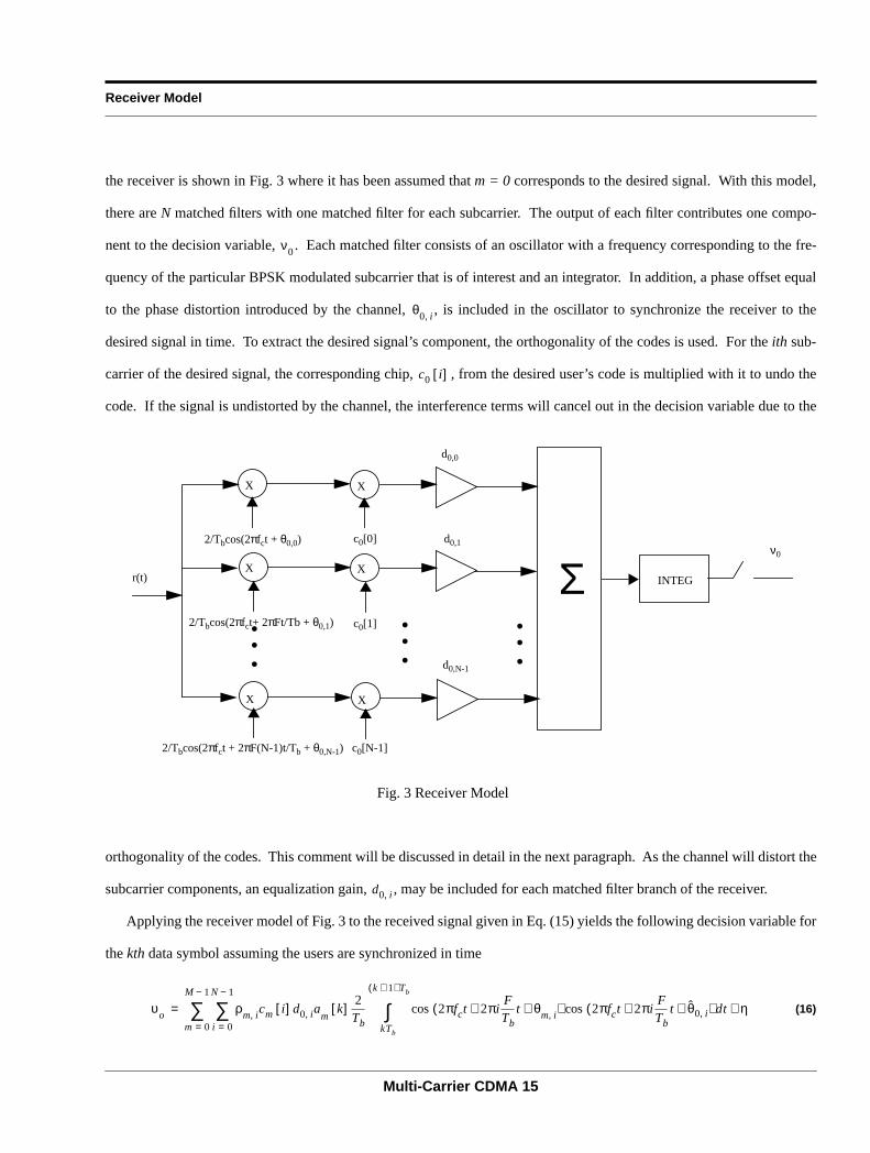
Multi-Carrier CDMA 15
the receiver is shown in Fig. 3 where it has been assumed thatm = 0 corresponds to the desired signal. With this model,
there areN matched filters with one matched filter for each subcarrier. The output of each filter contributes one compo-
nent to the decision variable, . Each matched filter consists of an oscillator with a frequency corresponding to the fre-
quency of the particular BPSK modulated subcarrier that is of interest and an integrator. In addition, a phase offset equal
to the phase distortion introduced by the channel,, is included in the oscillator to synchronize the receiver to the
desired signal in time. To extract the desired signal’s component, the orthogonality of the codes is used. For theith sub-
carrier of the desired signal, the corresponding chip, , from the desired user’s code is multiplied with it to undo the
code. If the signal is undistorted by the channel, the interference terms will cancel out in the decision variable due to the
orthogonality of the codes. This comment will be discussed in detail in the next paragraph. As the channel will distort the
subcarrier components, an equalization gain,, may be included for each matched filter branch of the receiver.
Applying the receiver model of Fig. 3 to the received signal given inEq. (15) yields the following decision variable for
thekth data symbol assuming the users are synchronized in time
(16)
ν0
θ0 i,
c0 i[ ]
X
2/Tbcos(2πfct + θ0,0)
X
2/Tbcos(2πfct+ 2πFt/Tb +θ0,1)
X
d0,0
d0,1
d0,N-1
Fig. 3 Receiver Model
Σ INTEG
..
. ...
r(t)
2/Tbcos(2πfct + 2πF(N-1)t/Tb + θ0,N-1)
ν0
X
X
X
..
.
c0[N-1]
c0[1]
c0[0]
d0 i,
υo ρm i,i 0=
N 1−
∑ cm i[ ] d0 i, am
k[ ]2Tb
2πfct 2πiFTb
+ t θm i,+( ) 2πfct 2πiFTb
+ t θ̂0 i,+( ) dtcos η+cos
kTb
k 1+( ) Tb
∫m 0=
M 1−
∑=
Principles of MC-CDMA
16 Multi-Carrier CDMA
where denotes the receiver’s estimation of the phase at theith subcarrier of the desired signal and the corresponding
AWGN term, , is given as
. (17)
Assuming perfect phase correction, i.e., , the decision variable reduces to
(18)
where . Note that if and are iid uniform r.v.’s on the interval [0, ], then is also uni-
formly distributed on the interval [0, ]. Note that the decision variable consists of three terms. The first term corre-
sponds to the desired signal’s component, the second corresponds to the interference and the last corresponds to a noise
term.
To illustrate the desired effect of the codes, consider the case of a perfect channel where and . In a
perfect channel, the decision variable is given as
(19)
where all interference terms cancel out because of the orthogonality of the codes. Unfortunately, in real multipath chan-
nels, this is unlikely to happen and each subcarrier will experience fading. This leads to the question of what form of
equalization should be performed.
3.9 Equalization
The question of what equalization technique should be used must address different issues. The underlying goal of
these techniques should be to reduce the effect of the fading and the interference while not enhancing the effect of the
noise on the decision of what data symbol was transmitted. Whenever there is a diversity scheme involved whether it may
involve receiving multiple copies of a signal from time, frequency or antenna diversity, the field of classical diversity the-
ory can be applied. These equalization techniques may be desirable for their simplicity as they involve simple multiplica-
tions with each copy of the signal. However, they may not be optimal in a channel with interference in the sense of
minimizing the error under some criterion. In some ways, these equalization scheme appear "ad hoc" as they are not
derived under some clear procedure.
θ̂0 i,
η
η n t( )2Tb
d0 i, 2πfct 2πiFTb
+ t θ̂0 i,+( ) dtcos
kTb
k 1+( ) Tb
∫i 0=
N 1−
∑=
θ̂0 i, θ0 i,=
υo a0. k[ ] ρ0 i, d0 i,i 0=
N 1−
∑ am k[ ] cm i[ ] c0 i[ ] ρm i, d0 i, θ̃m i,cosi 0=
N 1−
∑m 1=
M 1−
∑ η+ +=
θ̃m i, θ0 i, θm i,−= θ0 i, θm i, 2π θ̃m i,
2π
ρm i, 1= θm i, 0=
υo Na0. k[ ] am k[ ] cm i[ ] c0 i[ ]i 0=
N 1−
∑m 1=
M 1−
∑ η+ +=

Equalization
Multi-Carrier CDMA 17
It should be noted that while there are some decision making techniques, such as Viterbi decoding and Wiener filter-
ing, that are optimal in the sense that they minimize the mean-squared error, the actual implementation of these methods
may be prohibitive complex for a channel equivalent to the one that is being analyzed in this document. By assuming that
the fading at the N subcarriers are independent, it is assumed that there are N degrees of freedom in one form or another.
This channel assumption could imply that there are N resolvable paths in a DS-CDMA rake receiver. It could mean that
there are N taps in the impulse response of the channel and a very large number of states in a Viterbi decoder for large N.
It could also mean there are N taps in a LMS implementation of a Wiener filter.
In the analysis, three equalization techniques will be evaluated: Equal Gain Combining (EGC), Maximal Ratio Com-
bining (MRC) and Controlled Equalization (CE). These techniques may be associated with classical diversity theory as
they involved multiplying each copy of the signal by some gain factor as shown in Fig. 3. As it can be seen from Eq. (17),
each of the equalization techniques will affect the distribution of the noise component differently. In Appendix A, the sta-
tistical characteristics of the noise for the different equalization techniques are discussed.
3.9.1 EGC
With EGC, the gain factor of the ith subcarrier is chosen to be
, (20)
that is, this technique does not attempt to equalize the effect of the channel distortion in any way. This technique may be
desirable for its simplicity as the receiver does not require the estimation of the channel’s transfer function. Using this
scheme, the decision variable of Eq. (18) is given as
(21)
where the noise can be approximated by a zero-mean Gaussian random with a variance of
. (22)
3.9.2 MRC
With MRC, the scheme squares the amplitude of each copy of the signal by using a gain factor for the ith subcarrier of
. (23)
d0 i, 1=
υo a0. k[ ] ρ0 i,i 0=
N 1−
∑ am k[ ] cm i[ ] c0 i[ ] ρm i, θ̃m i,cosi 0=
N 1−
∑m 1=
M 1−
∑ η+ +=
ση2 N
N0
Tb=
d0 i, ρ0 i,=

Principles of MC-CDMA
18 Multi-Carrier CDMA
The motivation behind Maximal Ratio Combining is that the components of the received signal with large amplitudes are
likely to contain relatively less noise. Thus, their effect on the decision process is increased by squaring their amplitudes.
The corresponding decision variable is
(24)
where the noise can be approximated by a zero-mean Gaussian random variable with variance
. (25)
3.9.3 Controlled Equalization
While EGC may be desirable for its simplicity and MRC for its noise combating capability, neither of these techniques
directly address the interference and the exploitation of the coding at the subcarriers. As one of the goal of mobile radio
communication systems is to multiplex as many users as possible to share the same resources, the channel models for
these communication systems are moving from noise-limited channels to interference-limited channels. With CE, an
attempt at restoring the orthogonality between users is made by normalizing the amplitudes of the subcarriers. As the
orthogonality of the users is encoded in the phase of the subcarriers, this method appears to be primarily beneficial in the
downlink where phase distortion for all users may be more easily corrected rather than in the uplink. For Controlled
Equalization, the gain factor the ith subcarrier is
(26)
where is the unit step function. Thus, only subcarriers above a certain threshold will be equalized and retained.
This constraint is added to prevent the over amplification of subcarriers with small amplitudes that may be dominated by a
noise component. Given that there are subcarriers above the threshold, the corresponding decision variable is
(27)
where the inner sum of the interference term (indexed by j) is carried over the terms corresponding to the subcarriers
above threshold and
. (28)
υo a0. k[ ] ρ0 i,2
i 0=
N 1−
∑ am k[ ] cm i[ ] c0 i[ ] ρm i, ρ0 i, θ̃m i,cosi 0=
N 1−
∑m 1=
M 1−
∑ η+ +=
ση2 N
N0
TbEρ0 i,
2=
d0 i,1
ρ0 i,u ρ0 i, ρthresh−( )=
u ρ0 i,( )
n0
υo n0 a0. k[ ] n0 am k[ ] cm j[ ] c0 j[ ]j
∑m 1=
M 1−
∑ η+ +=
n0
η do j, n t( )2Tb
2πfct 2πjFTb
+ t θ0 j,+( ) dtcos
kTb
k 1+( ) Tb
∫j
∑=
Equalization
Multi-Carrier CDMA 19
The noise can be approximated by a zero-mean Gaussian random variable with a variance of
. (29)ση n0
2 n0
N0
TbEd0 j,
2=

Analysis of the Performance of MC-CDMA in Rayleigh and Rician Fading Channels
20 Multi-Carrier CDMA
CHAPTER 4 Analysis of the Performance ofMC-CDMA in Rayleigh andRician Fading Channels
4.1 Rayleigh Fading
4.1.1 Channel Model
In this section, the scalings of the amplitude are assumed to be independent and identically distributed (IID) Rayleigh ran-
dom variables of the form
(30)
where the indexes m and i have been added to differentiate between the mth user and the ith subcarrier. This corresponds
to the case in which the LOS path from the transmitter to the receiver is obstructed by a person or an object. The phase
effects, for i = 0, 1, ... N-1, introduced by the channel are assumed to be IID random variables uniformly distributed
on the interval [ , ] for all subcarriers. As summarized in Eq. (13), the local-mean power of one subcarrier is assumed
to be
with each user having a total local-mean power of .
fρm i,ρm i,( )
ρm i,
σm i,2
e
ρm i,2
2σm i,2
−
=
θm i,
π− π
pm i,12
Eρm i,2 σm i,
2= =
pm Npm i,=
Rayleigh Fading
Multi-Carrier CDMA 21
4.1.2 Uplink
For uplink transmissions, we will consider only EGC and MRC for the following reason. As mentioned above, for
uplink transmissions, phase correction is not simultaneously applied to the interference when it is applied to the desired
signal. Examining the interference component of the decision variable for EGC and MRC in Eq. (21) and in Eq. (24), the
phase distortion results in the multiplicative term . This term can add a phase of 0 or depending on the value of
which happens to be random. As the code is encoded in the phase, the phase distortion will randomize the phase and
consequently cancel the effect of the orthogonal coding unless predistortion is applied in the transmitters of the interfering
signals.
4.1.2.1 EGC
For EGC in the uplink, as explained below, the interference term
(31)
is a Gaussian r.v. Since the in-phase component of a Rayleigh random variable, , is Gaussian and
, consists of the sum of iid Gaussian r.v.’s. Thus, is Gaussian with a
mean and variance (as calculated in Appendix B) of
. (32)
Examining Eq. (21), the probability of making a decision error conditioned on the amplitudes of the desired signal,
, and the local-mean interference power, , given is
. (33)
Note that since is assumed to take on values of 1 and -1 with equal probability, the average probability of making a
decision error is equal to the bit error rate (BER). As the interference term and the noise term are independent and Gaus-
sian, the sum to the right of the inequality has a zero-mean Gaussian distribution with a variance equal to the sum of their
variances. Using this observation, the probability of a decision error can be found to be
. (34)
θ̃m i,cos π
θ̃m i,
βint am k[ ] cm i[ ] c0 i[ ] ρm i, θ̃m i,cosi 0=
N 1−
∑m 1=
M 1−
∑=
ρm i, θ̃m i,cos
am k[ ] cm i[ ] c0 i[ ] 1 1,−{ }∈ βint M 1−( ) N× βint
Eβint 0= σβint
2 M 1−( ) pm=
ρ0 i,{ }i 0=N 1− σβint
2 a0 k[ ] 1−=
Pr error ρ0 i,{ }i 0=N 1− σβint
2,( ) Pr ρ0 i, βint η+<i 0=
N 1−
∑ =
am k[ ]
Pr error ρ0 i,{ }i 0=N 1− σβint
2,( )1
2π σβint
2 σn2+( )
e
y2
2 σβint
2 σn2+( )
−
dy
ρ0 i,
i 0=
N 1−
∑
∞
∫=

Analysis of the Performance of MC-CDMA in Rayleigh and Rician Fading Channels
22 Multi-Carrier CDMA
Performing a change of variables results in
(35)
where the complementary error function is defined to be
. (36)
To obtain an expression for the average probability of making a decision error, Eq. (35) must be averaged over the distri-
bution of the instantaneous amplitudes .
Finding the distribution of the sum of iid Rayleigh random variables
(37)
has historically been a difficult problem. In [16], Beaulieu offers an infinite series representation of this sum that has some
computational advantages. In this paper, three approximations of the distribution will be compared: a Law of Large Num-
bers (LLN) approximation, a small parameter approximation [16], and a Central Limit Theorem (CLT) approximation.
1. LLNIn the limiting case of a large number of subcarriers, can be approximated by the LLN to be the constant .
The advantage of using the LLN is that it requires low computational complexity. Using the LLN simplifies the expres-
sion for the probability of error to
. (38)
Applying the statistical properties of Rayleigh distributions given in Eq. (4), the probability of error simplifies to
. (39)
2. Small Argument Approximation
For small values of , the distribution of can be approximated by
Pr error ρ0 i,{ }i 0=N 1− pm,( )
12
erfc
12
ρ0 i,i 0=
N 1−
∑
2
M 1−( ) pm
NN0
Tb+
=
erfc x( )2
πe t2− dt
x
∞
∫≡
ρ0 i,{ }i 0=N 1−
ρ0 ρ0 i,i 0=
N 1−
∑=
ρ0 i,i 0=
N 1−
∑ NEρo i,
Pr error Eρ0 i, pm,( )12
erfc
12
N2E2ρ0 i, Tb
M 1−( ) pmTb NN0+
≅
Pr error p0 pm,( )12
erfcπ4
p0Tb
M 1−( )pm
NTb N0+
≅
ρ0 ρ0
Rayleigh Fading
Multi-Carrier CDMA 23
(40)
where . In contrast to the LLN approximation, is considered to be a random variable instead of
a deterministic constant. Thus, the average probability of making a decision error may be approximated by averaging
over Eq. (40) to yield
. (41)
3. CLT
A third possible approximation can be obtained by applying the CLT for the limiting case of large N. Using the CLT
results in a BER of
(42)
where and . This expression may be simplified by exchanging the order of the integrals to
yield
. (43)
Thus, the randomness of the desired signals’ amplitudes may be reflected as an addition to the power of the interference
and noise and consequently is a more conservative approximation than the LLN approximation.
4.1.2.2 MRC
For MRC, the interference component is given as
. (44)
Comparing Eq. (44) with Eq. (31), it can be seen that for MRC and EGC, the interference components have similar forms.
Thus, the analysis for MRC should follow the analysis of EGC. Since consists of iid r.v.’s with respect
to m and i, it can be approximated by a zero-mean Gaussian r.v. with a variance as determined in Appendix B of
f ρ0 p0( )ρ0
2N 1− e
ρ02
2b−
2N 1− bN N 1−( ) !=
bp0
N2N 1−( ) ! ![ ] 1 N⁄= ρ0
Pr error p0 pm,( )ρ0
2N 1− e
ρ02
2b−
2N 1− bN N 1−( ) !
12
erfc
12
ρ02Tb
M 1−( ) pmTb NN0+
dρ00
∞
∫≅
Pr error p0 pm,( )1
2πσρ0
2e
ρ0 µρ0
−( )
2σρ0
2
2
−12
erfc
12
ρ02Tb
M 1−( ) pmTb NN0+
dρ0∞−
∞
∫≅
µρ0
π2
Np0= σρ0
2 2π2
−( ) p0=
Pr error p0 pm,( )12
erfcπ4
p0Tb
2π2
−( )p0
NTb M 1−( )
pm
NTb N0+ +
≅
βint am k[ ] cm i[ ] c0 i[ ] ρm i, ρ0 i, θ̃m i,cosi 0=
N 1−
∑m 1=
M 1−
∑=
βint M 1−( ) N×
Analysis of the Performance of MC-CDMA in Rayleigh and Rician Fading Channels
24 Multi-Carrier CDMA
. (45)
Using Eq. (24) Eq. (25) Eq. (45), the conditioned instantaneous BER for MRC can be calculated to be
. (46)
1. ExactFortunately, the distribution of the sum of exponentially distributed random variables is known to have the
gamma distribution which has the following closed form distribution
. (47)
Unconditioning Eq. (46) over Eq. (47) results in the following exact expression for the average probability of error using
MRC
. (48)
2. LLN
Using Eq. (48) as a basis of comparison, the expressions of the probability of error for the LLN and CLT will be included
so that the effectiveness of the EGC approximations can be judged. Using the LLN, the probability of error is given as
. (49)
3. CLT
Using the CLT approximation with and , the probability of error can be found to be
. (50)
σβint
2 2M 1−( )
Npmp0=
Pr error ρ0 i,{ }i 0=N 1− p0 pm, ,( )
12
erfc
12
ρ0 i,2
i 0=
N 1−
∑
2
2M 1−( )
Npmp0
2p0N0
Tb+
=
r12
ρ0 i,
2
i 0=
N 1−
∑=
f r p0( )1
p0 i, N 1−( ) !
r
p0 i,
N 1−e
r
p0 i,
−
=
Pr error p0 pm,( )1
p0 i, N 1−( ) !
r
p0 i,
N 1−e
r
p0 i,
−12
erfcr2Tb
M 1−( )N
pmp0Tb p0N0
+
dr
0
∞
∫=
Pr error p0 pm,( )12
erfcp0T
b
M 1−( )N
pmTb N0+
≅
µ 2p0= σ 4p0
2
N=2
Pr error p0 pm,( )12
erfcp0T
b
2p0
NTb
M 1−( )N
+ pmTb N0+
≅

Rayleigh Fading
Multi-Carrier CDMA 25
4.1.3 Downlink
As discussed earlier, downlink transmissions designated for different users arrive at one particular receiver through the
same channel. Thus, in this section, we will use the notation of Eq. (14) and assume perfect phase correction for the inter-
ference. The generalized decision variable given in Eq. (18) simplifies to
. (51)
Note that in contrast to the uplink, the sign reversals due to phase distortions are no longer present in the interference term.
Thus, the effect of the subcarrier coding is not invalidated by the channel and can be included in the analysis. Let
. (52)
Note that the orthogonality of the codes described in Eq. (8)
(53)
for and the fact that imply that the set consists of exactly elements that are
equal to "1" and exactly elements that equal to "-1". Let the elements of set that are equal to "1" be indexed by
and the elements that are equal to "-1" be indexed by for = 0, 1, ..., such that
. (54)
Using this notation, the generalized decision variable in the downlink may be written as
. (55)
4.1.3.1 EGC
Using Eq. (55), the decision variable for EGC is given as
(56)
where the interference now has a variance of
. (57)
υo a0. k[ ] ρ0 i, d0 i,i 0=
N 1−
∑ am k[ ] cm i[ ] c0 i[ ] ρ0 i, d0 i,i 0=
N 1−
∑m 1=
M 1−
∑ η+ +=
Q i[ ] cl i[ ] cm i[ ]=
Q i[ ]i 0=
N 1−
∑ 0=
l m≠ Q i[ ] 1 1,−{ }∈ A Q i[ ]{ } i 0=N 1−= N
2N2
A aj
bj jN2
1−
Q aj[ ] 1= Q bj[ ] 1−=
aj{ } bj{ }∪ 0 1 … N 1−, , ,{ }=
υo a0. k[ ] ρ0 i, d0 i,i 0=
N 1−
∑ am k[ ] ρ0 aj, d0 aj, ρ0 bj,j 0=
N
21−
∑ d0 bj,−j 0=
N
21−
∑
m 1=
M 1−
∑ η+ +=
υo a0. k[ ] ρ0 i,i 0=
N 1−
∑ am k[ ] ρ0 aj, ρ0 bj,j 0=
N
21−
∑−j 0=
N
21−
∑m 1=
M 1−
∑ η+ +=
σβint
2 2 M 1−( ) 1π4
− p0=
Analysis of the Performance of MC-CDMA in Rayleigh and Rician Fading Channels
26 Multi-Carrier CDMA
Following an analysis similar to that of the uplink and using Eq. (22) and Eq. (57), the average BER for EGC in the down-
link can be obtained for the following approximations
1. LLN
(58)
2. Small Argument
(59)
3. CLT
With and , the BER can be expressed as
. (60)
Comparing Eq. (58) with Eq. (60), it can be seen that using the CLT approximation is more conservative, resulting in "1"
additional interfering power compared to the LLN approximation.
4.1.3.2 MRC
The decision variable for MRC in the downlink is
(61)
where from Appendix B the interference has a variance of
. (62)
Following an analysis similar to that of the uplink and using Eq. (25) and Eq. (62), the average BER for MRC in the
downlink can be obtained for the following approximations
1. Exact
(63)
2. LLN
Pr error p0( )12
erfcπ4
p0Tb
2M 1−( )
N1
π4
− p0Tb N0+
≅
Pr error p0( )ρ0
2N 1− e
ρ02
2b−
2N 1− bN N 1−( ) !
12
erfc
12
ρ02Tb
2 M 1−( ) 1π4
−( ) p0Tb NN0+
dρ00
∞
∫≅
µρ0
π2
Np0= σρ0
2 2π2
−( ) p0=
Pr error p0( )12
erfcπ4
p0Tb
2MN
1π4
− p0Tb N0+
≅
υo a0. k[ ] ρ0 i,2
i 0=
N 1−
∑ am k[ ] ρ0 aj,2 ρ0 bj,
2
j 0=
N
21−
∑−j 0=
N
21−
∑m 1=
M 1−
∑ η+ +=
σβint
2 M 1−N
( ) 4p02=
Pr error p0( )1
p0 i, N 1−( ) !
r
p0 i,
N 1−e
r
p0 i,
−12
erfcr2Tb
2M 1−( )
Np0
2Tb p0N
0+
dr
0
∞
∫=

Rayleigh Fading
Multi-Carrier CDMA 27
(64)
3. CLT
Using the CLT approximation with and , the probability of error can be found to be
. (65)
4.1.3.3 Controlled Equalization (CE)
Examining Eq. (27), the probability of making a decision error conditioned the number of subcarriers above the
threshold, , and the interference component, , given is
(66)
where the variance of the noise, , is given in Eq. (A-10) as
(67)
where is the exponential integral defined as
(68)
and the probability that a subcarrier is above the threshold for Rayleigh fading is
. (69)
The distribution of the number of subcarriers above the threshold, , is described by the following binomial distribution
(70)
for = 0, 1, 2, ... , N. As mentioned earlier, note that the orthogonality of the codes, given by the following condition
, (71)
imply that half of the inner products, , are positive while the other half are negative. Denote the inner sum of
the interference term of Eq. (27) by
Pr error p0( )12
erfcp0T
b
2M 1−( )
Np0Tb N0+
≅
µ 2p0= σ2 4p0
2
N=
Pr error p0( )12
erfcp0T
b
2MN
p0Tb N0+
≅
n0 βint a0 k[ ] 1−=
Pr error n0 βint,( )1
2πση n0
2e
x2
2ση n0
2−
dx
n0 βint−
∞
∫≅
ση n0
2
ση n0
2 n0
N0
Tb
1
2p0 i,
1pron
E1
ρthresh2
2p0 i, =
E1 ρ( )
E1 ρ( ) e t−
tdt
ρ
∞
∫=
pron e
ρthresh2
2p0 i,
−
=
n0
pn0n0( ) N
n0
pron{ } n0 1 pron−{ } N n0−=
n0
cm i[ ] c0 i[ ]i 0=
N 1−
∑ Nδm 0,=
cm i[ ] c0 i[ ]

Analysis of the Performance of MC-CDMA in Rayleigh and Rician Fading Channels
28 Multi-Carrier CDMA
. (72)
Using this notation, the distribution of the inner sum given that there are subcarriers above threshold is
(73)
where and can only assume even (odd) values if is even (odd). The exact
distribution of the interference term, , given depends on the spreading code, for i = 0, 1, ..., N-1. In this
analysis, it is assumed that each of the inner sums acts as an independent r.v., and that the pdf of the interference is given
as the convolution of the pdfs of for m = 1, 2, ..., M-1. Combining the results given above yield the following expres-
sion for the bit error rate
. (74)
4.2 Rician Fading
In an indoor environment, the direct path from the transmitter, which most likely is located on the ceiling, to the
receiving terminal is usually unobstructed. Thus, the Rician distribution given in Eq. (5) is more appropriate when
describing of the amplitude scalings, of the channel. To conform to the multi-carrier and multi-user notation, the
Rician distribution is rewritten as
(75)
where the indexes i and m have been added to differentiate between the ith subcarrier at the frequency and the
mth user. As the notation suggests, the dominant LOS component, , is assumed to equal for all subcarriers and all users.
With BPSK modulation, the power of the LOS component for "1" subcarrier is . The scattered power, , is also
assumed to be equal with respect to user m and subcarrier i. As a consequence, the Rician K-factor given in Eq. (6) and
rewritten here using the user/subcarrier notation
, (76)
is equal for users and subcarriers. The mean given in Eq. (7) can be rewritten as
Σm cm j[ ] c0 j[ ]j
∑=
n0
pΣm n0
Σm n0( )
N 2⁄n0 Σm+( ) 2⁄
N 2⁄n0 Σm−( ) 2⁄
Nn0
=
min n0 N, n0−{ }− Σm m≤ in n0 N n0−,{ }≤ Σm n0
βint n0 cm i[ ]{ }
Σm
BER pn0n0( ) pβint n0
βint n0( )12
erfcn0 βint−
2ση n0
βint
∑n0 0=
N
∑≅
ρm i,
fρm i,ρm i,( )
ρm i,
σm i,2
e
ρm i,2 b0
2+
2σm i,2
−
I0
b0ρm i,
σm i,2
=
f0 Fi
Tb+
bo
12
b02 σm i,
2
Kb0
2
2σm i,2
=

Rician Fading
Multi-Carrier CDMA 29
. (77)
Assuming BPSK modulation, the local-mean power of the ith subcarrier of the mth user consisting of a contribution from
the scattered component and the LOS component is defined to be
. (78)
In terms of the Rician K-factor and the local-mean power, the power of the dominant and scattered components can be
rewritten as
. (79)
Consequently, the Rician pdf may be rewritten in terms of the K-factor as
. (80)
4.2.1 Uplink
The method for obtaining the BER with Rician fading is identical to that of Rayleigh fading with the same decision
variables being used. The only factors that change in the expressions are the replacement of the statistical properties of
Rayleigh fading with Rician fading. The calculation of the statistical properties of the interference assuming Rician fad-
ing are included in Appendix B. To obtain the average BER, the conditional expressions that are obtained must be aver-
aged over the sum of Rician r.v.’s or of Rician-squared r.v.’s. Again, the difficulty of finding closed form expressions for
the distribution of these r.v.’s are encountered. Again, the LLN and CLT will be used to approximate the average BER.
While it is theoretically possible to synchronize the transmitters in time so that the LOS components will maintain their
orthogonality and cancel out of the decision variable, it can be shown that this scenario would require a time synchroniza-
tion of within which may not be feasible for high bit rates or large . Thus, this case is not considered.
4.2.1.1 EGC
With EGC in a Rician fading channel, the variance of the interference is given in Appendix B as
. (81)
The average BER for the LLN and CLT approximations are
1. LLN
Eρm i, e K 2⁄− π2 K 1+( )
p0 i, 1 K+( ) I0K2
( ) KI1K2
( )+=
pm i, E ρm i, 2πfct 2πiFTb
+ t θm i,+( )cos2 1
2Eρm i,
2 σm i,2 1
2b0
2+= = =
12
b02 K
K 1+pm i,= σm i,
2 pm i,
K 1+=
fρm i,ρm i, K pm i,,( ) K 1+( ) e K−
ρm i,
pm i,
e
K 1+
2pm i,
ρm i,2−
I0 ρm i,2K K 1+( )
pm i, =
Tb N⁄ N
σβint
2 M 1−( ) pm=
Analysis of the Performance of MC-CDMA in Rayleigh and Rician Fading Channels
30 Multi-Carrier CDMA
(82)
where
. (83)
2.
Applying the CLT with and results in
. (84)
4.2.1.2 MRC
With MRC in the uplink of a Rician fading channel, the variance of the interference is given in Appendix B as
. (85)
The BER expressions that result are as follows.
1. LLN
(86)
2. CLT
Applying the CLT with and results in
. (87)
4.2.2 Downlink
4.2.2.1 EGC
Approximating the interference by a Gaussian distribution, the variance of can be determined to be
. (88)
The corresponding average BER expressions are as follows.
1. LLN
Pr error p0 K,( )12
erfcγp0T
b
M 1−N
( ) pmTb N0+
≅
γπ4
e K−
K 1+( ) 1 K+( ) I0
K2
( ) KI1K2
( )+2
=
µρ02Nγp0= σρ0
2 2 1 γ−( ) p0=
Pr error p0 pm K, ,( )12
erfcγp0Tb
2 1 γ−[ ]p0
NTb
M 1−N
pmTb N0+ +
≅
σβint
2 2M 1−( )
Npmp0=
Pr error p0 K,( )12
erfcp0T
b
M 1−N
( ) pmTb N0+
≅
µr 2p0= σr2 8K 4+
K 1+( ) 2
p02
N=
Pr error p0 K,( )12
erfcp0T
b
4K 2+
K 1+( ) 2
p0
NTb
M 1−N
pmTb N0+ +
≅
βint
σβint
2 2 M 1−( ) 1 γ−( ) p0=

Rician Fading
Multi-Carrier CDMA 31
(89)
2. CLT
Applying the CLT with and results in
. (90)
4.2.2.2 MRC
Approximating the interference by a Gaussian distribution, the variance of can be determined to be
. (91)
The resulting average BER expressions are given below.
1. LLN
(92)
2. CLT
Applying the CLT with and results in
. (93)
Note that for all the average BER expressions obtained assuming Rician fading, the expressions for K = 0 reduce to that of
Rayleigh fading agreeing with earlier results.
4.2.2.3 CE
With CE in a Rician fading channel, only two factors will change from the Rayleigh fading case. As mentioned in Appen-
dix A, the variance of the noise given that there are subcarriers above threshold is now given as
(94)
where
Pr error p0 K,( )12
erfcγp0T
b
2M 1−
N( ) 1 γ−[ ] p0Tb N0+
≅
µρ02Nγp0= σρ0
2 2 1 γ−( ) p0=
Pr error p0 K,( )12
erfcγp0Tb
2MN
1 γ−[ ] p0Tb N0+
≅
βint
σβint
2 M 1−N
( )8K 4+K 1+( ) 2
p02=
Pr error p0 K,( )12
erfcp0T
b
M 1−N
( )4K 2+
K 1+( ) 2p0Tb N0+
≅
µr 2p0= σr2 8K 4+
K 1+( ) 2
p02
N=
Pr error p0 K,( )12
erfcp0T
b
MN
4K 2+
K 1+( ) 2p0Tb N0+
≅
n0
ση n0
2 n0
N0
Tb
1
2p0 i,
1pron
K 1+( ) e K− 1
ρo i, p0 i,
e
K 1+
2p0 i,
ρ0 i,2−
I0 ρ0 i,2K K 1+( )
p0 i, dρ0 i,
ρthresh
∞
∫=

Analysis of the Performance of MC-CDMA in Rayleigh and Rician Fading Channels
32 Multi-Carrier CDMA
. (95)
The distribution of the number of subcarriers above the threshold, , remains a binomial distribution but with a different
binomial parameter, . The average BER expression remains the same as Eq. (74).
pron K 1+( ) e K−ρo i,
p0 i,
e
K 1+
2p0 i,
ρ0 i,2−
I0 ρ0 i,2K K 1+( )
p0 i, dρ0 i,
ρthresh
∞
∫=
n0
pron

Rayleigh Fading
Multi-Carrier CDMA 33
CHAPTER 5 Numerical Results
In the analytical section, the only closed form expressions for the average BER were obtained with MRC. In this sec-
tion, approximations for the BER using the LLN and the CLT will be evaluated numerically. These results will be com-
pared to the exact results for MRC to measure the reliability of these approximations.
5.1 Rayleigh Fading
5.1.1 Uplink
Using the expressions for the BER obtained for uplink transmissions in a Rayleigh fading channel, the average BER
versus the number of co-channel interferers with a spreading factor of is shown in Fig. 4. To calculate the BER,
it is assumed that the local-mean power of each interferer is equal to the local-mean power of the desired signal. The SNR,
which is assumed to be 10dB, is defined to be
. (96)
Eq. (39), Eq. (41), and Eq. (43) correspond to the BER expressions for the LLN, the small argument, and the CLT
approximations using EGC in the receiver. While Eq. (49) and Eq. (50) give the LLN and CLT approximations for
MRC, Eq. (48) gives an exact expression for the BER. As it can be seen in Fig. 4., the approximations for MRC give rel-
atively close results when compared to the exact result. Note that the exact results and the CLT approximation for MRC
are indistinguishable. This observation indicates that the CLT approximation may be better than the LLN. For EGC, all
of approximations give results that are close to the other approximations. For all approximations, it can be seen the MRC
N 128=
SNRp0Tb
N0=
Numerical Results
34 Multi-Carrier CDMA
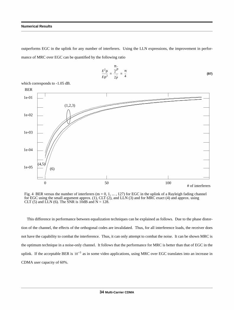
outperforms EGC in the uplink for any number of interferers. Using the LLN expressions, the improvement in perfor-
mance of MRC over EGC can be quantified by the following ratio
(97)
which corresponds to -1.05 dB.
This difference in performance between equalization techniques can be explained as follows. Due to the phase distor-
tion of the channel, the effects of the orthogonal codes are invalidated. Thus, for all interference loads, the receiver does
not have the capability to combat the interference. Thus, it can only attempt to combat the noise. It can be shown MRC is
the optimum technique in a noise-only channel. It follows that the performance for MRC is better than that of EGC in the
uplink. If the acceptable BER is as in some video applications, using MRC over EGC translates into an increase in
CDMA user capacity of 60%.
E2ρ
Eρ2
π2
p
2p
π4
= =
BER
# of interferers
Fig. 4 BER versus the number of interferers (m = 0, 1, ... , 127) for EGC in the uplink of a Rayleigh fading channelfor EGC using the small argument approx. (1), CLT (2), and LLN (3) and for MRC exact (4) and approx. usingCLT (5) and LLN (6). The SNR is 10dB and N = 128.
1e-05
1e-04
1e-03
1e-02
1e-01
0 50 100
(4,5)
(1,2,3)
(6)
10 3−
Rayleigh Fading
Multi-Carrier CDMA 35
5.1.2 Downlink
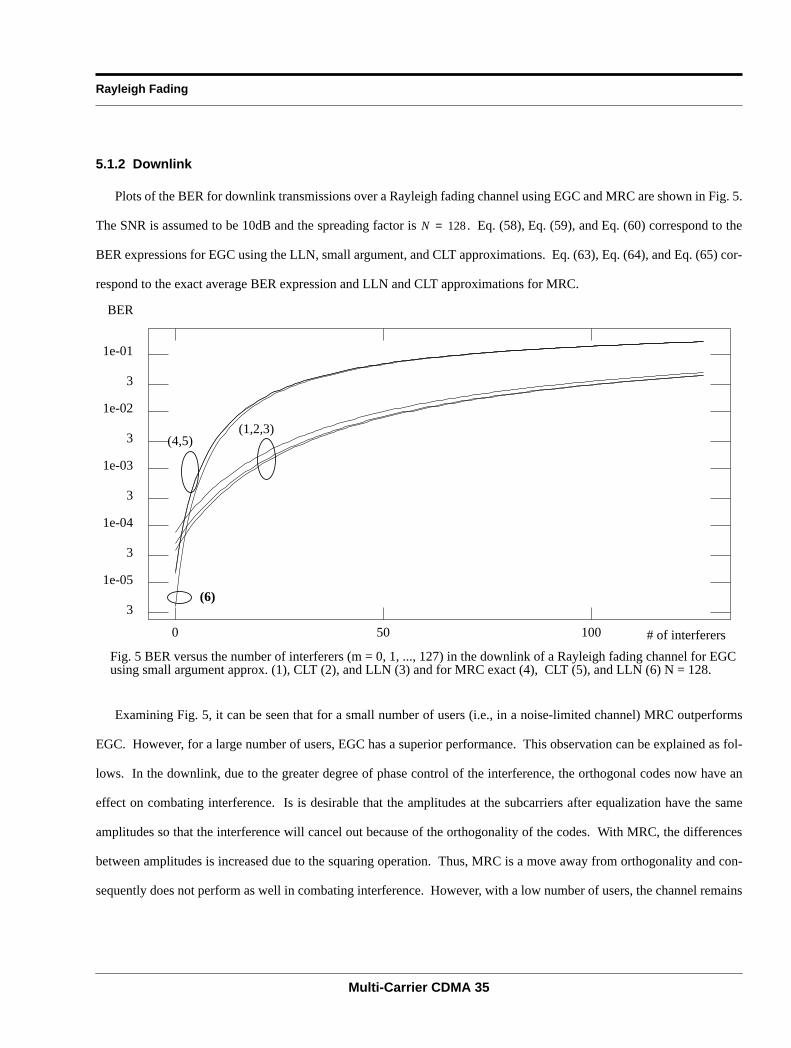
Plots of the BER for downlink transmissions over a Rayleigh fading channel using EGC and MRC are shown in Fig. 5.
The SNR is assumed to be 10dB and the spreading factor is . Eq. (58), Eq. (59), and Eq. (60) correspond to the
BER expressions for EGC using the LLN, small argument, and CLT approximations. Eq. (63), Eq. (64), and Eq. (65) cor-
respond to the exact average BER expression and LLN and CLT approximations for MRC.
Examining Fig. 5, it can be seen that for a small number of users (i.e., in a noise-limited channel) MRC outperforms
EGC. However, for a large number of users, EGC has a superior performance. This observation can be explained as fol-
lows. In the downlink, due to the greater degree of phase control of the interference, the orthogonal codes now have an
effect on combating interference. Is is desirable that the amplitudes at the subcarriers after equalization have the same
amplitudes so that the interference will cancel out because of the orthogonality of the codes. With MRC, the differences
between amplitudes is increased due to the squaring operation. Thus, MRC is a move away from orthogonality and con-
sequently does not perform as well in combating interference. However, with a low number of users, the channel remains
N 128=
(4,5)(1,2,3)
BER
# of interferers
Fig. 5 BER versus the number of interferers (m = 0, 1, ..., 127) in the downlink of a Rayleigh fading channel for EGCusing small argument approx. (1), CLT (2), and LLN (3) and for MRC exact (4), CLT (5), and LLN (6) N = 128.
3
1e-05
3
1e-04
3
1e-03
3
1e-02
3
1e-01
0 50 100
(6)

Numerical Results
36 Multi-Carrier CDMA
a noise-limited channel and consequently, MRC performs better. Again, note that the exact results and the CLT approxi-
mation for MRC are indistinguishable.
In comparison to the uplink, the performance in the downlink is better when the same equalization technique is com-
pared. Comparing the performance of EGC in the uplink to the downlink at a bit error rate of , there is an increase in
capacity from 8 users to 20 users in the downlink. This improvement is due to the greater degree of phase control in the
downlink that allows for some of the benefits from the orthogonality of the codes to be utilized.
Plots of the BER for CE in the downlink of a Rayleigh fading channel for a SNR of 10dB and 20dB are shown in Fig.
6 and Fig. 7. The expression for the BER with CE is given in Eq. (74). The BER curves are calculated for different values
of the threshold power to local-mean power (TLR) per subcarrier, which is defined to be
. (98)
Note that for large N, a SNR of 10dB results in a very small SNR at each subcarrier and a threshold power lower than the
power of the noise. Plots of the performance for EGC and MRC using the LLN approximation are included for compari-
son. With CE, the performance also depends on the local-mean power of the desired signal which was chosen to be
.
As it can be seen from Fig. 6, there exists threshold levels, , in which CE outperforms EGC and MRC for a high
number of users. This observation is due to the interference combating capability of CE. Note that there exists a
such that the BER versus the number of interferers is relatively flat. At this threshold level, there are a sufficient number
of subcarriers above the threshold such that orthogonality between users has been significantly restored. As the threshold
level is lowered past this point, no benefit occurs since "orthogonality" has been already been achieved and only noise
amplification results. For higher threshold values, the BER is affected by the number of interferers to a greater extent.
Note that for all threshold levels, CE performs worse than EGC or MRC for a low number of users. This degradation is
the trade-off between combating interference and combating noise. In restoring the orthogonality between users and com-
bating interferers, the noise has also been amplified.
Although CE outperforms EGC and MRC in the downlink, the BER that is achievable with CE in a Rayleigh fading
channel is still very high (on the order of ) for a SNR of 10dB. With a low SNR, CE suffers greatly from the amplifi-
10 3−
TLR
12
ρthresh2
p0 N⁄=
p0 0.1=
ρthresh
ρthresh
10 2−

Rayleigh Fading
Multi-Carrier CDMA 37
cation of the noise. If a SNR of 20dB is used, as shown in Fig. 7, acceptable BERs on the order of are obtainable.
With the larger SNR, CE suffers less from noise amplification.
In the downlink, the following trend is observed. For a very low number of users, MRC outperforms all equalization
techniques. This observation is in agreement with theory since MRC is the optimum equalization technique in a noise-
limited channel. As the number of users is increased, EGC becomes the best equalization technique out of all the methods
considered. Although the interference increases, the increase is not great enough to balance the adverse effects of noise
amplification that CE experiences. As the load is increased past a certain point, CE becomes the best equalization tech-
nique in the interference-limited channel.
1e-05
1e-04
1e-03
1e-02
1e-01
0 50 100
(1)
(2)
(3,4,5,6)
BER
# of interferers
Fig. 6 BER versus the number of interferers (m = 0, 1, ..., 127) in the downlink of a Rayleigh fading channel forMRC (1), EGC (2), and CE for TLR = -16.3 dB (3), TLR = -13.8 dB (4), TLR =-10.3 dB (5), and TLR = -6.8 dB.The SNR is 10dB, p0 = 0.1, and N = 128.
10 8−

Numerical Results
38 Multi-Carrier CDMA
5.2 Rician Fading
5.2.1 Uplink
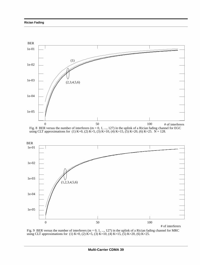
Plots of the average BER versus the number of interferers in the uplink of a Rician fading channel using EGC and
MRC are shown in Fig. 8 and Fig. 9 for K = 0, 5, 10, 15, and 25. The BER expressions are given in Eq. (84) and Eq. (87).
Only the CLT approximations have been included to prevent the cluttering of the curves since the LLN results are almost
identical. Note that without the coding of the subcarriers (due to the lack of phase control in the uplink) the K-factor has
little effect in the uplink.
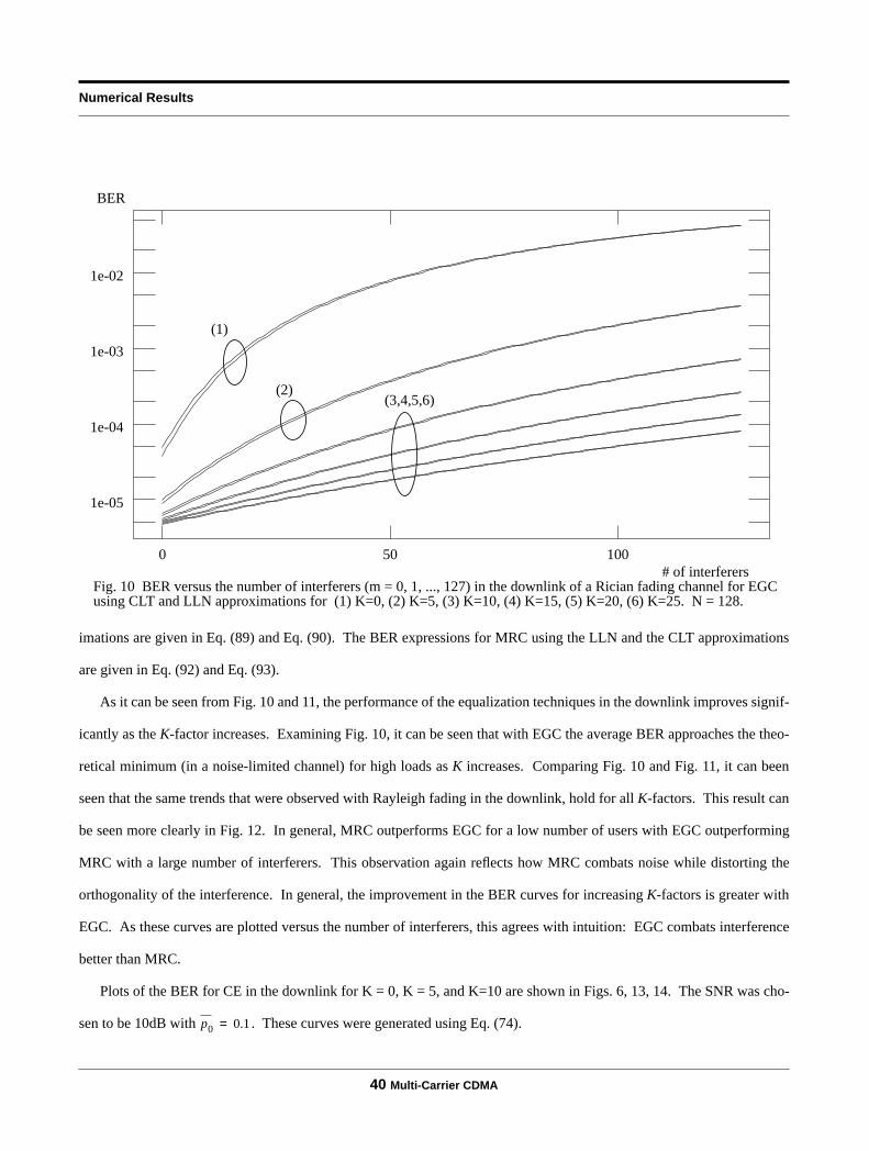
5.2.2 Downlink
Plots of the BER using EGC and MRC in the downlink of a Rician fading channel for various K-factors are shown in
Fig. 10 and Fig. 11. A third plot that combines the curves of EGC and MRC for K = 0 and K = 10 is included so that the
two frequency equalization techniques can be compared. The BER expressions for EGC using the LLN and CLT approx-
BER
1e-22
1e-20
1e-18
1e-16
1e-14
1e-12
1e-10
1e-08
1e-06
1e-04
1e-02
1e+00
0 50 100
(1)(2)
(3,4,5,6)
# of interferers
Fig. 7 BER versus the number of interferers (m = 0, 1, ..., 127) in the downlink of a Rayleigh fading channelfor MRC (1), EGC (2), and CE for TLR = -33.8 dB (3), TLR = -28.4 dB (4), TLR = -25.9 dB (5), and TLR =-19.9 dB. (6). The SNR is 20dB, p0 = 0.1, and N = 128.
Rician Fading
Multi-Carrier CDMA 39
1e-05
1e-04
1e-03
1e-02
1e-01
0 50 100Fig. 8 BER versus the number of interferers (m = 0, 1, ..., 127) in the uplink of a Rician fading channel for EGCusing CLT approximations for (1) K=0, (2) K=5, (3) K=10, (4) K=15, (5) K=20, (6) K=25. N = 128.
BER
# of interferers
(1)
(2,3,4,5,6)
1e-05
1e-04
1e-03
1e-02
1e-01
0 50 100
BER
# of interferersFig. 9 BER versus the number of interferers (m = 0, 1, ..., 127) in the uplink of a Rician fading channel for MRCusing CLT approximations for (1) K=0, (2) K=5, (3) K=10, (4) K=15, (5) K=20, (6) K=25.
(1,2,3,4,5,6)
Numerical Results
40 Multi-Carrier CDMA
imations are given in Eq. (89) and Eq. (90). The BER expressions for MRC using the LLN and the CLT approximations
are given in Eq. (92) and Eq. (93).
As it can be seen from Fig. 10 and 11, the performance of the equalization techniques in the downlink improves signif-
icantly as the K-factor increases. Examining Fig. 10, it can be seen that with EGC the average BER approaches the theo-
retical minimum (in a noise-limited channel) for high loads as K increases. Comparing Fig. 10 and Fig. 11, it can been
seen that the same trends that were observed with Rayleigh fading in the downlink, hold for all K-factors. This result can
be seen more clearly in Fig. 12. In general, MRC outperforms EGC for a low number of users with EGC outperforming
MRC with a large number of interferers. This observation again reflects how MRC combats noise while distorting the
orthogonality of the interference. In general, the improvement in the BER curves for increasing K-factors is greater with
EGC. As these curves are plotted versus the number of interferers, this agrees with intuition: EGC combats interference
better than MRC.
Plots of the BER for CE in the downlink for K = 0, K = 5, and K=10 are shown in Figs. 6, 13, 14. The SNR was cho-
sen to be 10dB with . These curves were generated using Eq. (74).
1e-05
1e-04
1e-03
1e-02
0 50 100
(1)
(2)(3,4,5,6)
BER
Fig. 10 BER versus the number of interferers (m = 0, 1, ..., 127) in the downlink of a Rician fading channel for EGC# of interferers
using CLT and LLN approximations for (1) K=0, (2) K=5, (3) K=10, (4) K=15, (5) K=20, (6) K=25. N = 128.
p0 0.1=

Rician Fading
Multi-Carrier CDMA 41
BER
1e-05
1e-04
1e-03
1e-02
1e-01
0 50 100
(1)(2,3,4,5,6)
Fig. 11 BER versus the number of interferers (m=0, 1, ..., 127) in the downlink of a Rician fading channel for MRC# of interferers
using CLT and LLN approximations for (1) K=0, (2) K=5, (3) K=10, (4) K=15, (5) K=20, (6) K=25. N = 128.
Fig. 12 BER versus the number of interferers (m = 0, 1, ..., 127) for different Rician K-factors using MRC:# of interferers
BER
1e-05
1e-04
1e-03
1e-02
1e-01
0 50 100
(1)
(2)
(3)
(4)
K=0 (1) and K=10 (3) and EGC: K=0 (2) and K=10 (4). Curves are shown for both CLT and LLN approximations.The SNR is 10 dB and N = 128.
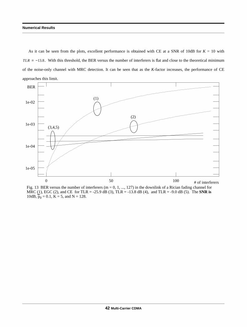
Numerical Results
42 Multi-Carrier CDMA
As it can be seen from the plots, excellent performance is obtained with CE at a SNR of 10dB for K = 10 with
. With this threshold, the BER versus the number of interferers is flat and close to the theoretical minimum
of the noise-only channel with MRC detection. It can be seen that as the K-factor increases, the performance of CE
approaches this limit.
TLR 13.8−=
1e-05
1e-04
1e-03
1e-02
0 50 100
(1)
(2)
(3,4,5)
BER
Fig. 13 BER versus the number of interferers (m = 0, 1, ..., 127) in the downlink of a Rician fading channel for# of interferers
MRC (1), EGC (2), and CE for TLR = -25.9 dB (3), TLR = -13.8 dB (4), and TLR = -9.0 dB (5). The SNR is10dB, p0 = 0.1, K = 5, and N = 128.
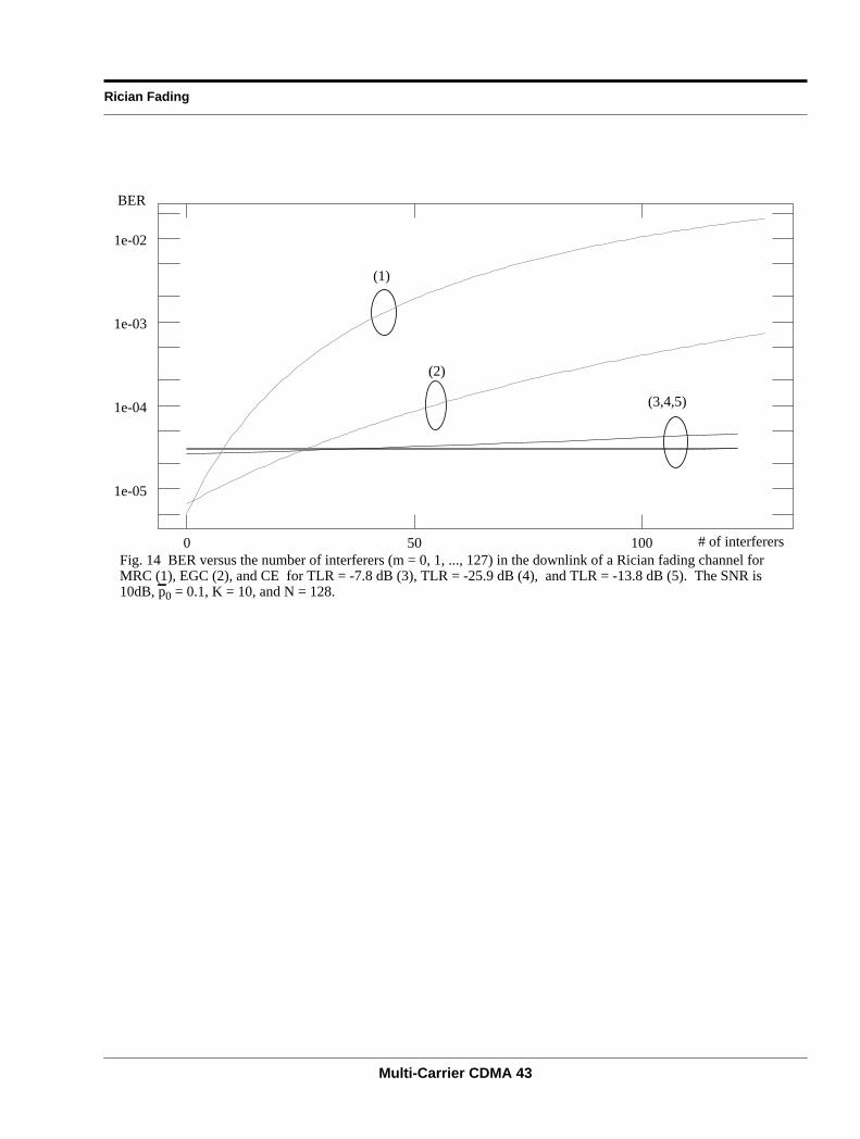
Rician Fading
Multi-Carrier CDMA 43
1e-05
1e-04
1e-03
1e-02
0 50 100
(1)
(2)
(3,4,5)
BER
Fig. 14 BER versus the number of interferers (m = 0, 1, ..., 127) in the downlink of a Rician fading channel for# of interferers
MRC (1), EGC (2), and CE for TLR = -7.8 dB (3), TLR = -25.9 dB (4), and TLR = -13.8 dB (5). The SNR is10dB, p0 = 0.1, K = 10, and N = 128.

Conclusion
44 Multi-Carrier CDMA
CHAPTER 6 Conclusion
In this document, a novel digital modulation technique called Multi-Carrier Code Division Multiple Access was intro-
duced and analyzed in both Rayleigh and Rician fading channels. The performance of this technique, gauged by the aver-
age bit error rate, was analytically and numerically evaluated for three equalization techniques that fall under classical
diversity techniques. These techniques, Equal Gain Combining, Maximal Ratio Combining, and Controlled Equalization,
perform equalization in the frequency domain, taking the component of each subcarrier (which represents the fading of
the channel at a corresponding frequency) and performing a multiplicative operation on this component.
MC-CDMA appears to be a new promising spread spectrum-multiple access technique. It appears to be most effective
in the downlink where phase control is most easily implemented. In the downlink, it was found that CE outperforms EGC
and MRC in combating interference. It can also operate well in channels with large delay spreads: an assumption of inde-
pendent fading at the subcarriers corresponds to a DS-CDMA system in which the number of resolvable paths is equal to
the spreading factor. Since the F-parameter can be freely chosen, the spacing between subcarriers can be chosen so that
MC-CDMA will exploit frequency diversity without excessive spreading factors.
In the uplink of a MC-CDMA communications system, it was found that because of the lack of phase control the
codes and the orthogonality between users is invalidated. As the effectiveness of CE depends on restoring the orthogonal-
ity between users, it was not considered in the uplink. Thus, unless a remedy is applied to compensate for this deficiency,
the coding of the subcarriers has no effect and consequently, the equalization techniques that were considered have no
ability to combat the interference besides the redundancy in transmissions at multiple subcarriers. Thus, as one would
expect, MRC, which is the optimal equalization in a noise-only channel, outperforms EGC. A possible solution to the
phase distortion problem is predistortion in the transmitters. With this technique, each transmitter makes a measurement

Rician Fading
Multi-Carrier CDMA 45
of the channel and modifies the signal that it transmits so that at the receiving end, the signal that is obtained is the original
signal that it intended to transmit.
For downlink transmissions, the following pattern was observed. For a very low number of users, MRC outperforms
all equalization techniques. This result agrees with intuition since this corresponds to a noise-limited channel. For inter-
ference-limited channels, CE outperforms all techniques. This results because CE makes a direct attempt at combating
interference. In between these two extremes, EGC performed the best for a "medium" load. While not distorting the
orthogonality between users as with MRC and while not over amplifying the noise as with CE, EGC finds the balance
between these extremes.
Thus, these equalization techniques have two conflicting goals: to combat noise and to combat interference. In the
process of combating one form of degradation, the receiver becomes more susceptible to the other. EGC may be desirable
for its simplicity, MRC in systems where a low number of users are expected, and CE for interference-limited channels. It
should be noted that future communication systems tend to be headed in the direction of interference-limited channels, as
they attempt to multiplex as many users as possible using the same resources.
While these techniques are not optimal in the sense that they do not address the minimization of some performance
parameter, they are noteworthy for their relative simplicity and their intuitive feel for the underlying effects of the coding
of the subcarriers. It should be noted that although CE is not optimal, it produces low BERs that are close to the theoreti-
cal minimum that are obtainable in a noise-only Rician fading channel (using MRC) with K = 10. A more formal (and
more complicated) approach may be taken with multi-signal/multi-user detection to minimize the interference plus noise
power in the decision process. With these schemes, each receiver considers the signals designated for all users simulta-
neously to decide what was transmitted from the desired user.
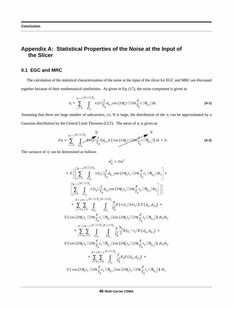
Conclusion
46 Multi-Carrier CDMA
Appendix A: Statistical Properties of the Noise at the Input ofthe Slicer
0.1 EGC and MRC
The calculation of the statistical characterization of the noise at the input of the slicer for EGC and MRC are discussed
together because of their mathematical similarities. As given in Eq. (17), the noise component is given as
. (A-1)
Assuming that there are large number of subcarriers, i.e, N is large, the distribution of the can be approximated by a
Gaussian distribution by the Central Limit Theorem (CLT). The mean of is given as
. (A-2)
The variance of can be determined as follows
η n t( )2Tb
d0 i, 2πfct 2πiFTb
+ t θ0 i,+( ) dtcos
kTb
k 1+( ) Tb
∫i 0=
N 1−
∑=
η
η
Eη En t( )2Tb
Ed0 i, E 2πfct 2πiFTb
+ t θ0 i,+( )cos{ } dt
kTb
k 1+( ) Tb
∫i 0=
N 1−
∑ 0= =
00
η
ση2 Eη2=
E n t1( )2Tb
d0 i, 2πfct1 2πiFTb
+ t1 θ0 i,+( ) dt1cos
kTb
k 1+( ) Tb
∫i 0=
N 1−
∑ ×
=
n t2( )2Tb
d0 j, 2πfct2 2πjFTb
+ t2 θ0 j,+( ) dt2cos
kTb
k 1+( ) Tb
∫j 0=
N 1−
∑
4
Tb2
E n t1( ) n t2( ){ } E d0 i, d0 j,{ }kTb
k 1+( ) Tb
∫kTb
k 1+( ) Tb
∫j 0=
N 1−
∑i 0=
N 1−
∑ ×=
E 2πfct1 2πiFTb
+ t1 θ0 i,+( ) 2πfct2 2πjFTb
+ t2 θ0 j,+( )coscos{ } dt1dt2
4
Tb2
N0
2δ t1 t2−( ) E d0 i, d0 j,{ }
kTb
k 1+( ) Tb
∫kTb
k 1+( ) Tb
∫j 0=
N 1−
∑i 0=
N 1−
∑ ×=
E 2πfct1 2πiFTb
+ t1 θ0 i,+( ) 2πfct2 2πjFTb
+ t2 θ0 j,+( )coscos{ } dt1dt2
2
Tb2
N0E d0 i, d0 j,{ }kTb
k 1+( ) Tb
∫j 0=
N 1−
∑i 0=
N 1−
∑ ×=
E 2πfct1 2πiFTb
+ t1 θ0 i,+( ) 2πfct1 2πjFTb
t1+ θ0 j,+( )coscos{ } dt1
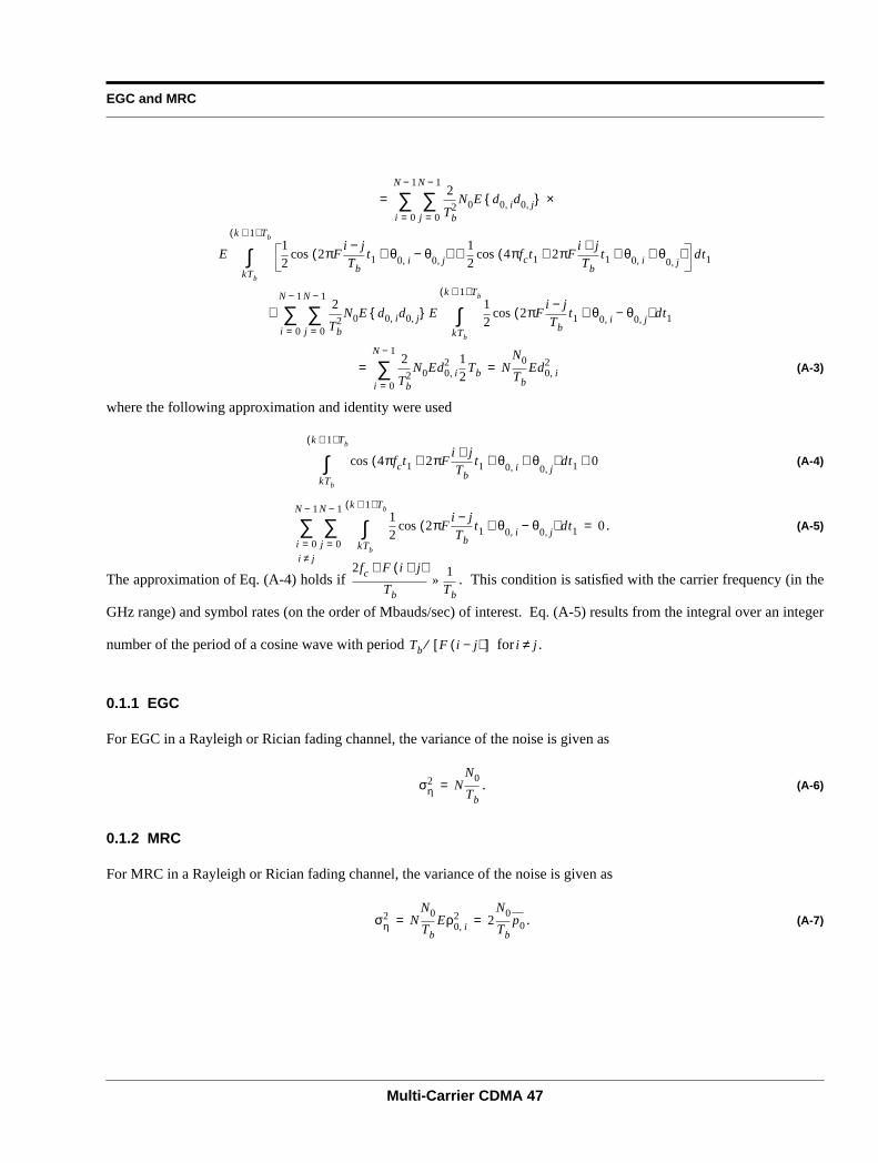
EGC and MRC
Multi-Carrier CDMA 47
(A-3)
where the following approximation and identity were used
(A-4)
. (A-5)
The approximation ofEq. (A-4) holds if . This condition is satisfied with the carrier frequency (in the
GHz range) and symbol rates (on the order of Mbauds/sec) of interest.Eq. (A-5) results from the integral over an integer
number of the period of a cosine wave with period for .
0.1.1 EGC
For EGC in a Rayleigh or Rician fading channel, the variance of the noise is given as
. (A-6)
0.1.2 MRC
For MRC in a Rayleigh or Rician fading channel, the variance of the noise is given as
. (A-7)
2
Tb2
N0E d0 i, d0 j,{ }j 0=
N 1−
∑i 0=
N 1−
∑ ×=
E12
2πFi j−Tb
t1 θ0 i, θ0 j,−+( )12
4πfct1 2πFi j+Tb
t1+ θ0 i, θ+0 j,
+( )cos+cos dt1kTb
k 1+( ) Tb
∫
2
Tb2
N0E d0 i, d0 j,{ }j 0=
N 1−
∑i 0=
N 1−
∑ E12
2πFi j−Tb
t1 θ0 i, θ0 j,−+( )cos dt1kTb
k 1+( ) Tb
∫≅
2
Tb2
N0Ed0 i,2
i 0=
N 1−
∑ 12
Tb NN0
TbEd0 i,
2= =
4πfct1 2πFi j+Tb
t1+ θ0 i, θ+0 j,
+( )cos dt1kTb
k 1+( ) Tb
∫ 0≅
12
2πFi j−Tb
t1 θ0 i, θ0 j,−+( )cos dt1kTb
k 1+( ) Tb
∫j 0=
N 1−
∑i 0=i j≠
N 1−
∑ 0=
2fc F i j+( )+
Tb
1Tb
»
Tb F i j−( )[ ]⁄ i j≠
ση2 N
N0
Tb=
ση2 N
N0
TbEρ0 i,
2 2N0
Tbp0= =
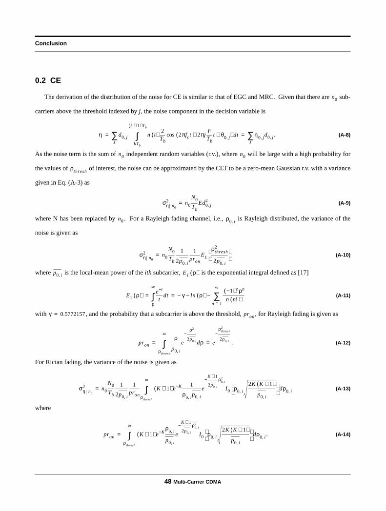
Conclusion
48 Multi-Carrier CDMA
0.2 CE
The derivation of the distribution of the noise for CE is similar to that of EGC and MRC. Given that there are sub-
carriers above the threshold indexed by j, the noise component in the decision variable is
. (A-8)
As the noise term is the sum of independent random variables (r.v.), where will be large with a high probability for
the values of of interest, the noise can be approximated by the CLT to be a zero-mean Gaussian r.v. with a variance
given in Eq. (A-3) as
(A-9)
where N has been replaced by . For a Rayleigh fading channel, i.e., is Rayleigh distributed, the variance of the
noise is given as
(A-10)
where is the local-mean power of the ith subcarrier, is the exponential integral defined as [17]
(A-11)
with , and the probability that a subcarrier is above the threshold, , for Rayleigh fading is given as
. (A-12)
For Rician fading, the variance of the noise is given as
(A-13)
where
. (A-14)
n0
η d0 j, n t( )2Tb
2πfct 2πjFTb
+ t θ0 j,+( ) dtcos
kTb
k 1+( ) Tb
∫j
∑ η0 j, d0 j,j
∑= =
n0 n0
ρthresh
ση n0
2 n0
N0
TbEd0 j,
2=
n0 ρ0 i,
ση n0
2 n0
N0
Tb
1
2p0 i,
1pron
E1
ρthresh2
2p0 i, =
p0 i, E1 ρ( )
E1 ρ( ) e t−
tdt
ρ
∞
∫ γ− ln ρ( )−1−( ) nρn
n n!( )n 1=
∞
∑−= =
γ 0.5772157= pron
pron
ρ
p0 i,
e
ρ2
2p0 i,
−
dρρthresh
∞
∫ e
ρthresh2
2p0 i,
−
= =
ση n0
2 n0
N0
Tb
1
2p0 i,
1pron
K 1+( ) e K− 1
ρo i, p0 i,
e
K 1+
2p0 i,
ρ0 i,2−
I0 ρ0 i,2K K 1+( )
p0 i, dρ0 i,
ρthresh
∞
∫=
pron K 1+( ) e K−ρo i,
p0 i,
e
K 1+
2p0 i,
ρ0 i,2−
I0 ρ0 i,2K K 1+( )
p0 i, dρ0 i,
ρthresh
∞
∫=

Uplink
Multi-Carrier CDMA 49
Appendix B: Statistical Properties of the Interference (at theInput to the Slicer)
The following statistical identities will be used
. (B-1)
0.1 Uplink
0.1.1 EGC
The interference component, , for EGC is given as
. (B-2)
Since the in-phase component of a Rayleigh random variable, , is Gaussian and ,
consists of the sum of iid Gaussian r.v.’s. Thus, is Gaussian with a mean of
(B-3)
and a variance of
. (B-4)
If has a Rician distribution, then the interference can be approximated by the CLT as a Gaussian r.v. since it consists
of a sum of iid r.v.’s. Thus, will have the same mean and variance expression as in Eq. (B-3) and Eq. (B-4). Note that
this is true for the variance of the interference since the local-mean power for Rayleigh and Rician fading are defined by
the same quantity
.
Eam k[ ]12
1−( )12
1( )+ 0= = Eam2 k[ ]
12
1−( ) 2 12
1( ) 2+ 1= =
Ecos2 θ0 i, θm i,−( )1
2πcos2θ̃m i, θ̃m i,d
0
2π
∫12
= =
βint
βint am k[ ] cm i[ ] c0 i[ ] ρm i, θ̃m i,cosi 0=
N 1−
∑m 1=
M 1−
∑=
ρm i, θ̃m i,cos am k[ ] cm i[ ] c0 i[ ] 1 1,−{ }∈
βint M 1−( ) N× βint
Eβint Ei 0=
N 1−
∑m 1=
M 1−
∑ am k[ ] ρm i, cm i[ ] c0 i[ ] θ̃m i,cos{ }=
Eam k[ ] cm i[ ] c0 i[ ] Eρm i, E θ̃m i,cosi 0=
N 1−
∑m 1=
M 1−
∑ 0= =
σβint
2 M 1−( ) NE am k[ ] ρm i, cm i[ ] c0 i[ ] θ̃m i,cos{ }2
=
M 1−( ) Ncm2 i[ ] c
02 i[ ] Eam
2 k[ ] Eρm i,2 Ecos2θ̃m i,=
12
M 1−( ) NEρm i,2 M 1−( ) pm= =
ρ0 i,
βint
pm i,12
Eρm i,2=

Conclusion
50 Multi-Carrier CDMA
0.1.2 MRC
For MRC, the interference component is given as
(B-5)
As is composed of iid r.v.’s, it can be approximated by a Gaussian distribution using the CLT for both
Rayleigh and Rician fading with a mean of
(B-6)
and a variance of
. (B-7)
0.2 Downlink
0.2.1 EGC
For downlink transmissions using EGC, the interference component is
(B-8)
Applying the CLT independently to both inner summations yields two identical Gaussian random variables. Thus,
may be approximated by a zero-mean Gaussian r.v. with a variance of
(B-9)
for Rayleigh fading and
(B-10)
for Rician fading, where
βint am k[ ] cm i[ ] c0 i[ ] ρm i, ρ0 i, θ̃m i,cosi 0=
N 1−
∑m 1=
M 1−
∑=
βint M 1−( ) N×
Eβint M 1−( ) NE am k[ ] ρm i, cm i[ ] c0 i[ ] θ̃m i,cos{ }=
M 1−( ) NE am k[ ]{ } cm i[ ] c0 i[ ] Eρm i, E θ̃m i,cos 0= =
σβint
2 M 1−( ) NE am k[ ] ρm i, ρ0 i, cm i[ ] c0 i[ ] θ0 i, θm i,−( )cos{ } 2=
M 1−( ) Ncm2 i[ ] c
02 i[ ] Eam
2 k[ ] Eρm i,2 Eρ0 i,
2 Ecos2 θ0 i, θm i,−( )=
12
M 1−( ) NEρm i,2 Eρ0 i,
2 2M 1−( )
Npmp0= =
βint am k[ ] ρ0 aj, ρ0 bj,j 0=
N
21−
∑−j 0=
N
21−
∑
m 1=
M 1−
∑=
βint
σβint
3 M 1−( ) Nσρ0 i,
2 M 1−( ) N Eρ0 i,2 E2ρ0 i,−( ) M 1−( ) N 2p0 i,
π2
p0 i,−( )= = =
2 M 1−( ) 1π4
−( ) p0=
σβint
3 M 1−( ) Nσρ0 i,
2 2 M 1−( ) 1 γ−( ) p0= =

Downlink
Multi-Carrier CDMA 51
. (B-11)
0.2.2 MRC
For MRC in the downlink, the decision variable is given as
. (B-12)
Applying the CLT in the same manner as with EGC, the interference can be approximated by a zero-mean Gaussian r.v.
with a variance of
(B-13)
for Rayleigh fading and
(B-14)
for Rician fading.
γπ4
e K−
K 1+( ) 1 K+( ) I0
K2
( ) KI1K2
( )+2
=
βint am k[ ] ρ0 aj,2 ρ0 bj,
2
j 0=
N
21−
∑−j 0=
N
21−
∑
m 1=
M 1−
∑=
σβint
2 M 1−( ) N Eρ0 i,4 Eρ0 i,
2( ) 2−[ ] M 1−( ) N 8p0 i,2
4p0 i,2−( )
M 1−N
( ) 4p02= = =
σβint
2 M 1−( ) N Eρ0 i,4 Eρ0 i,
2( ) 2−[ ]M 1−
N( )
8K 4+K 1+( ) 2
p02= =

Conclusion
52 Multi-Carrier CDMA
Appendix C: Simplification of CL T Expressions
Assume the conditional BER to have the following general form
. (C-1)
Assuming that has a Gaussian distribution with mean and variance , the average BER can be simplified as follows
(C-2)
. (C-3)
pr error ρ( )12
erfc
12
ρ2
σβint
2 ση2+
1
2π σβint
2 ση2+( )
e
y2
2 σβint
2 ση2+( )
−
dy
ρ
∞
∫= =
ρ µ σ2
BER1
2πσ2e
ρ µ−( ) 2
2σ2−
1
2π σβint
2 ση2+( )
e
y2
2 σβint
2 ση2+( )
−
dydρρ
∞
∫∞−
∞
∫=
1
2π( ) 2σ2 σβint
2 ση2+( )
e
ρ µ−( ) 2
2σ2
x ρ+( ) 2
2 σβint
2 ση2+( )
−−
dρdx
∞−
∞
∫0
∞
∫=
1
2π( ) 2σ2 σβint
2 ση2+( )
e
1
2σ2 σβint
2 ση2+( )
µ σβint
2 ση2+( ) xσ2−{ } 2
σβint
2 ση2+ σ2+
− µ2 σβint
2 ση2+( ) x2σ2+ +−
×0
∞
∫=
e
1
2σ2 σβint
2 ση2+( )
σβint
2 ση2+ σ2+ ρ
µ σβint
2 ση2+( ) xσ2−
σβint
2 ση2+ σ2+
−
2
−
dρdx
∞−
∞
∫×
1
2π σβint
2 ση2+ σ2+( )
e
1
2σ2 σβint
2 ση2+( )
µ σβint
2 ση2+( ) xσ2−{ } 2
σβint
2 ση2+ σ2+
− µ2 σβint
2 ση2+( ) x2σ2+ +−
dx
0
∞
∫=
1
2π σβint
2 ση2+ σ2+( )
e
1
2
x µ+( ) 2
σβint
2 ση2+ σ2+( )
−
dx
0
∞
∫=
1
πe t2− dt
µ
2 σβint
2 ση2+ σ2+( )
∞
∫=
12
erfc
12
µ2
σ2 σ+ βint
2 ση2+
=

References
Multi-Carrier CDMA 53
References
[1] N. Yee, J. P. Linnartz and G. Fettweis, “Multi-Carrier CDMA in Indoor Wireless Radio Networks,” ProceedingsPIMRC ’93, Yokohama, Japan, 1993, pp. 109-113.
[2] G. Fettweis, “Multi-Carrier Code Division Multiple Access (MC-CDMA): Basic Idea,” Technekron CommunicationSystems - Internal Report.
[3] K. Fazel and L. Papke, “On the Performance of Convolutionally - Coded CDMA/OFDM for Mobile CommunicationSystem,” Proceedings PIMRC ’93, Yokohama, Japan, 1993, pp. 468-472.
[4] Leonard J. Cimini, Jr., “Analysis and Simulation of a Digital Mobile Channel Using Orthogonal Frequency DivisionMultiplexing,” IEEE Transactions on Communications, vol. COM-33, pp. 665-6.
[5] Michel Alard and Roselyne Lassalle, “Principles of Modulation and Channel Coding for Digital Broadcasting forMobile Receivers,”EBU Review - Technical, no. 224, pp. 168-190, 1987.
[6] J. Proakis,Digital Communications, New York: McGraw-Hill, 1983, Ch. 4.
[7] R. Ganesh and K. Pahlavan, “Effects of Traffic and Local Movements on Multipath Characteristics of an IndoorRadio Channel,”Electronics Letters, vol. 26, no. 12, June 1990, pp. 810-12.
[8] S. Howard and K. Pahlavan, “Doppler Spread Measurements of the Indoor Radio Channel,”Electronic Letters, v. 26,no. 2, 1990, pp. 107-109.
[9] Robert Bultitude, "Measurement, Characterization and Modelling of Indoor 800/900 MHz Radio Channels for Digi-tal Communications,"IEEE Communications Magazine, v. 25, no. 6, pp. 5-12, June 1987.
[10] R. Bultitude, S. Mahmoud and W. Sullivan, “A Comparison of Indoor Radio Propagation Characteristics at 910 MHzand 1.75 GHz,”IEEE Journal on Selected Areas in Communications, vol. 7, no. 1, Jan. 1989, pp. 20-30.
[11] Adel A.M. Saleh and Reinaldo A. Venuezula, “A Statistical Model for Indoor Multipath Propagation,”IEEE Journalon Selected Areas in Communications, vol. SAC-5, no. 2, pp. 128-137, Feb. 1987.
[12] Thomas A. Sexton and Kaveh Pahlavan, “Channel Modeling and Adaptive Equalization of Indoor Radio Channels,”IEEE Journal on Selected Areas in Communications, vol. 7, no. 1, pp. 114-120, Jan. 1989.
[13] J. P. Linnartz,Narrowband Land-Mobile Networks, Artech House, Norwood MA, 1993.
[14] R. L. Pickholtz, D. L. Schilling and L.B. Milstein, “Theory of Spread-Spectrum Communications - A Tutorial,” IEEETransactions on Communications, COM-30, May 1982, pp.855-884.
[15] Rodger E. Zeimer and Roger L. Peterson,Digital communications and spread spectrum systems, New York: Mac-millan; London: Collier Macmillan, c1985.
[16] N. C. Beaulieu, “Infinite Series for the Computation of the Complementary Probability Distribution Function as aSum of Independent Random Variables and Its Application to the Sum of Rayleigh Random Variables,”IEEE Trans-actions on Communications, vol. 38, no. 9, Sept. 1990, pp. 1463-1474.
[17] M. Abramowitz and L. A. Stegun,Handbook of Mathematical Functions: with Formulas, Graphs, and MathematicalTables, New York: Dover Publications, 1970.