Multi-Bunch Feedback Systems

H . Schmickler, CERN, CAS 2017 Egham

Special thanks to Marco Lonza for leaving most of his slides and animations

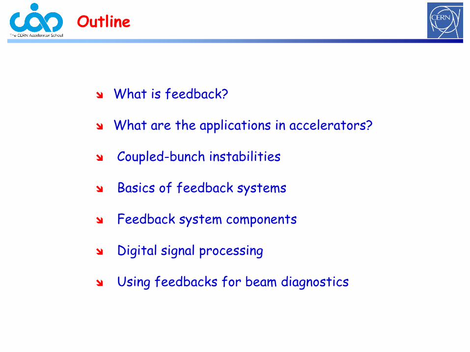
Outline

What is feedback?

What are the applications in accelerators?

Coupled-bunch instabilities

Basics of feedback systems

Feedback system components

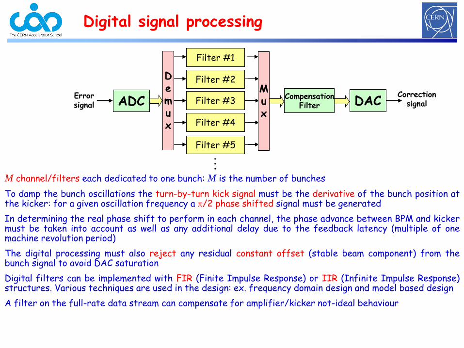
Digital signal processing

Using feedbacks for beam diagnostics

input

plant

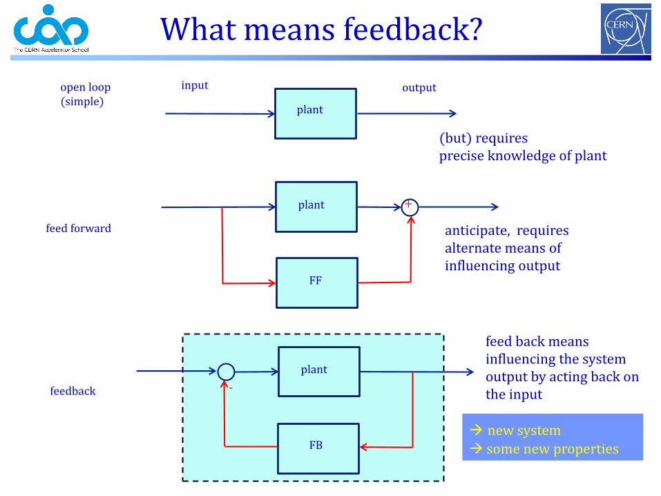
What means feedback?

open loop(simple)

(but) requiresprecise knowledge of plant

FF

output

plant

feed forward anticipate, requires alternate means of influencing output

+

FB

plant

feedback -

new system

some new properties

feed back means influencing the system output by acting back on the input

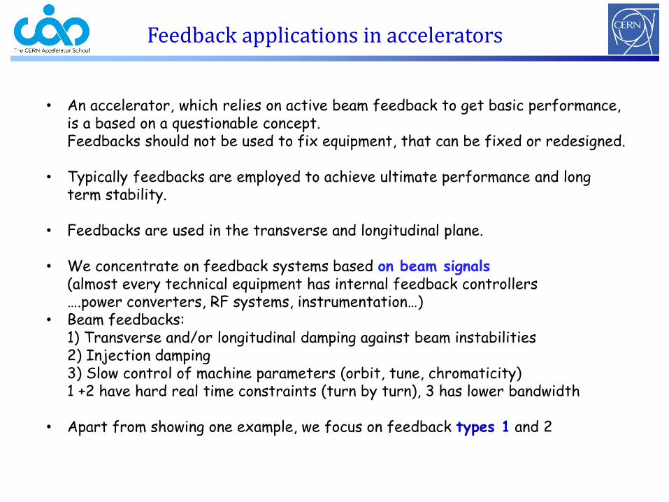
Feedback applications in accelerators

• An accelerator, which relies on active beam feedback to get basic performance, is a based on a questionable concept.Feedbacks should not be used to fix equipment, that can be fixed or redesigned.

• Typically feedbacks are employed to achieve ultimate performance and long term stability.

• Feedbacks are used in the transverse and longitudinal plane.

• We concentrate on feedback systems based on beam signals (almost every technical equipment has internal feedback controllers ….power converters, RF systems, instrumentation…)

• Beam feedbacks: 1) Transverse and/or longitudinal damping against beam instabilities2) Injection damping3) Slow control of machine parameters (orbit, tune, chromaticity)1 +2 have hard real time constraints (turn by turn), 3 has lower bandwidth

• Apart from showing one example, we focus on feedback types 1 and 2

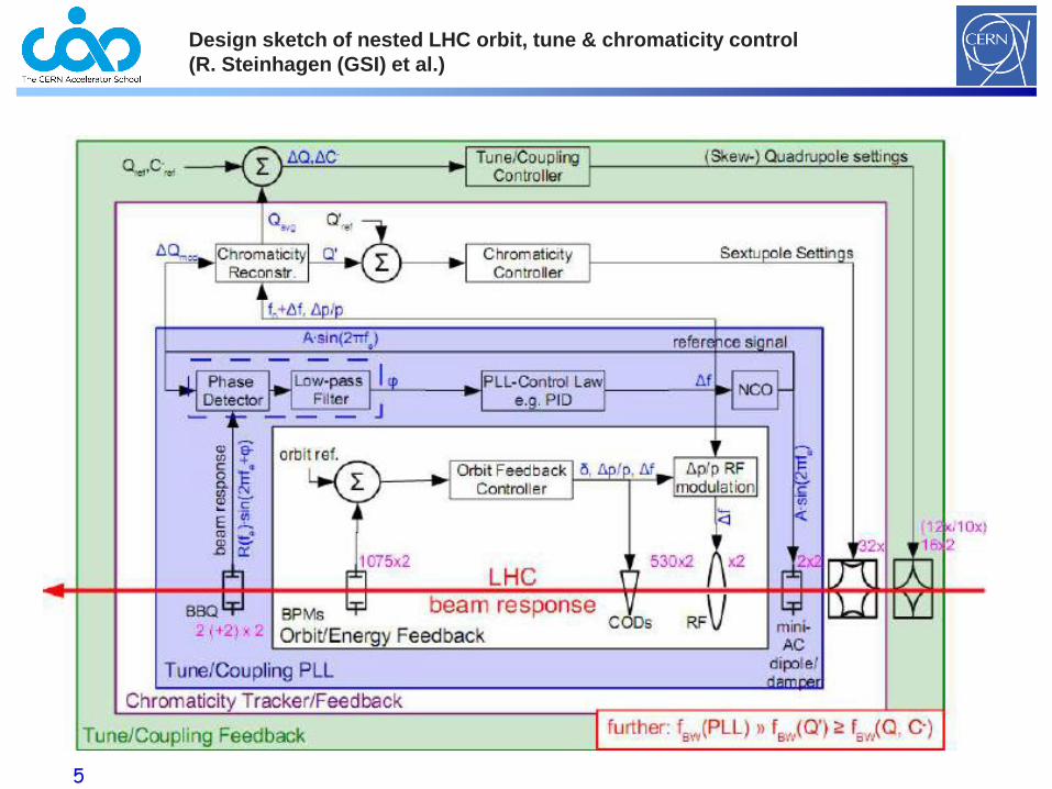
Design sketch of nested LHC orbit, tune & chromaticity control

(R. Steinhagen (GSI) et al.)

5

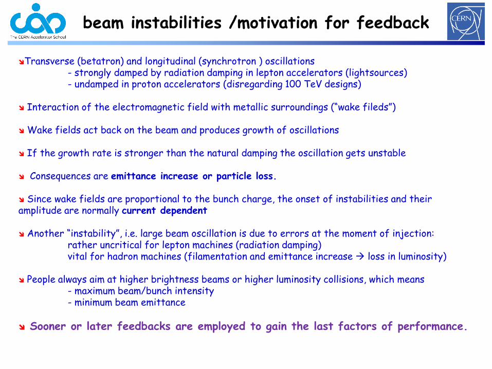
beam instabilities /motivation for feedback

Transverse (betatron) and longitudinal (synchrotron ) oscillations - strongly damped by radiation damping in lepton accelerators (lightsources)- undamped in proton accelerators (disregarding 100 TeV designs)

Interaction of the electromagnetic field with metallic surroundings (“wake fileds”)

Wake fields act back on the beam and produces growth of oscillations

If the growth rate is stronger than the natural damping the oscillation gets unstable

Consequences are emittance increase or particle loss.

Since wake fields are proportional to the bunch charge, the onset of instabilities and their amplitude are normally current dependent

Another “instability”, i.e. large beam oscillation is due to errors at the moment of injection:rather uncritical for lepton machines (radiation damping)vital for hadron machines (filamentation and emittance increase loss in luminosity)

People always aim at higher brightness beams or higher luminosity collisions, which means- maximum beam/bunch intensity- minimum beam emittance

Sooner or later feedbacks are employed to gain the last factors of performance.

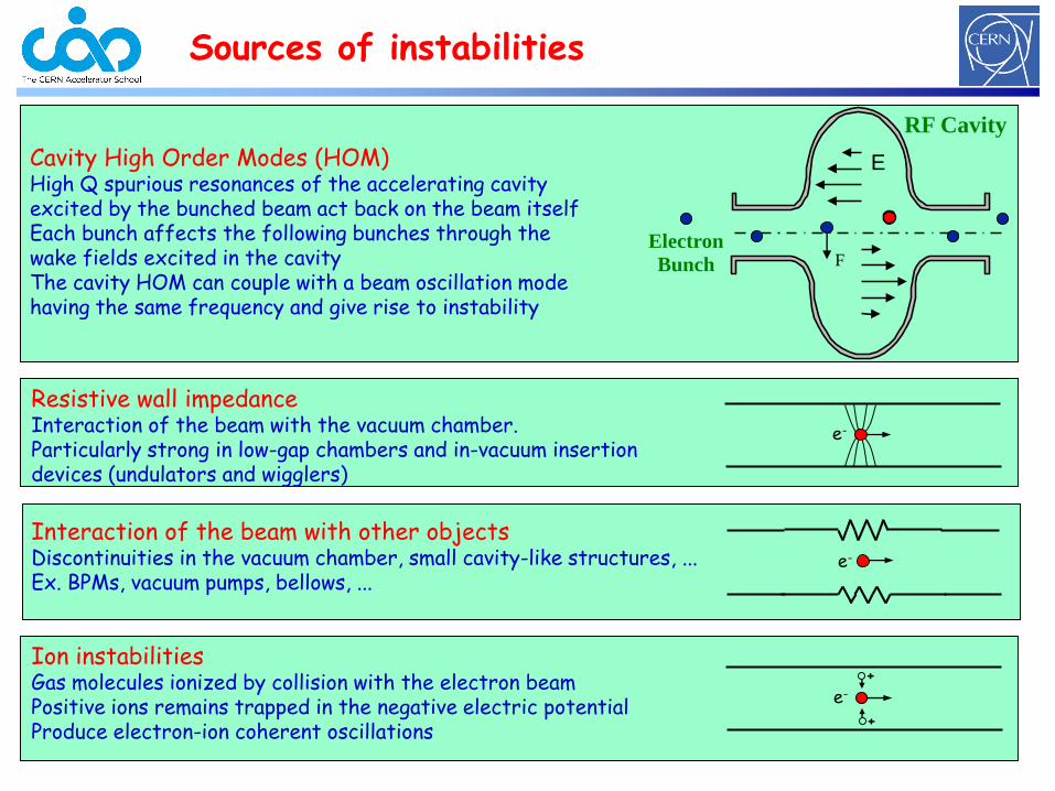
Sources of instabilities

Interaction of the beam with other objectsDiscontinuities in the vacuum chamber, small cavity-like structures, ... Ex. BPMs, vacuum pumps, bellows, ...

e-

Resistive wall impedanceInteraction of the beam with the vacuum chamber.Particularly strong in low-gap chambers and in-vacuum insertion devices (undulators and wigglers)

e-

Ion instabilitiesGas molecules ionized by collision with the electron beamPositive ions remains trapped in the negative electric potentialProduce electron-ion coherent oscillations

e-

+

+

Cavity High Order Modes (HOM)High Q spurious resonances of the accelerating cavity excited by the bunched beam act back on the beam itselfEach bunch affects the following bunches through the wake fields excited in the cavityThe cavity HOM can couple with a beam oscillation mode having the same frequency and give rise to instability

Electron

Bunch F

E

RF Cavity

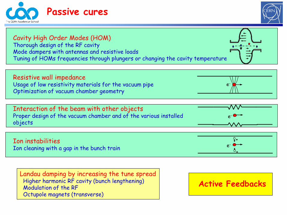
Passive cures

Landau damping by increasing the tune spreadHigher harmonic RF cavity (bunch lengthening)Modulation of the RFOctupole magnets (transverse)

Active Feedbacks

e-

e-

+

+

e-

Cavity High Order Modes (HOM)Thorough design of the RF cavityMode dampers with antennas and resistive loadsTuning of HOMs frequencies through plungers or changing the cavity temperature

Resistive wall impedanceUsage of low resistivity materials for the vacuum pipeOptimization of vacuum chamber geometry

Ion instabilitiesIon cleaning with a gap in the bunch train

Interaction of the beam with other objectsProper design of the vacuum chamber and of the various installed objects

H.Schmickler, CERN 9

H.Schmickler, CERN 10

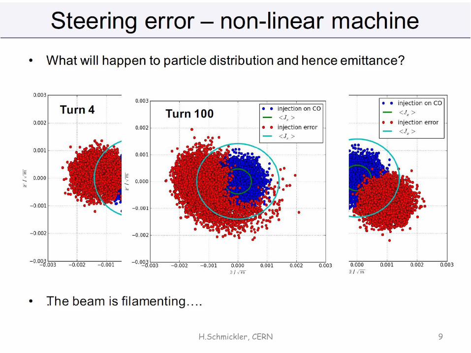
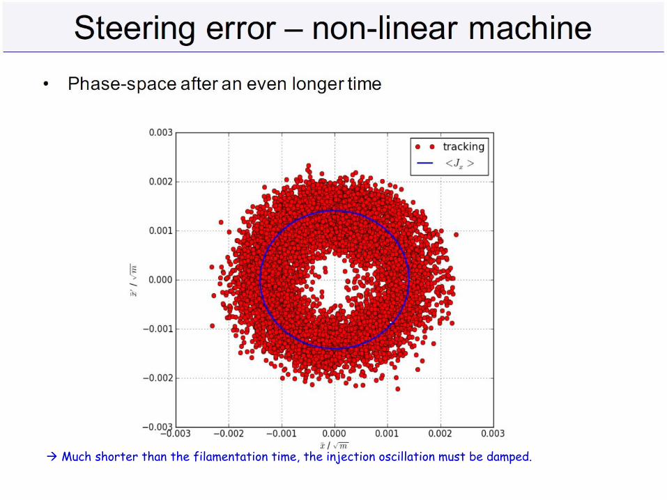
Much shorter than the filamentation time, the injection oscillation must be damped.

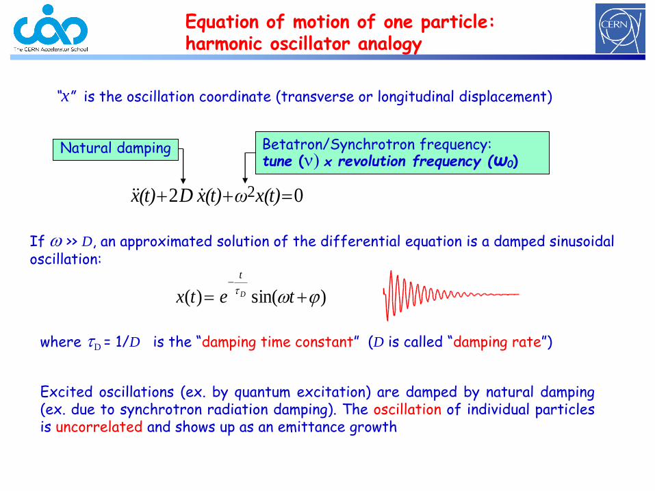
Equation of motion of one particle: harmonic oscillator analogy

02 2 x(t)ω(t)xD (t)x

Natural damping Betatron/Synchrotron frequency:tune (n) x revolution frequency (ω0)

Excited oscillations (ex. by quantum excitation) are damped by natural damping(ex. due to synchrotron radiation damping). The oscillation of individual particlesis uncorrelated and shows up as an emittance growth

)sin()(

tetx D

t

If >> D, an approximated solution of the differential equation is a damped sinusoidal oscillation:

where D = 1/D is the “damping time constant” (D is called “damping rate”)

“x” is the oscillation coordinate (transverse or longitudinal displacement)

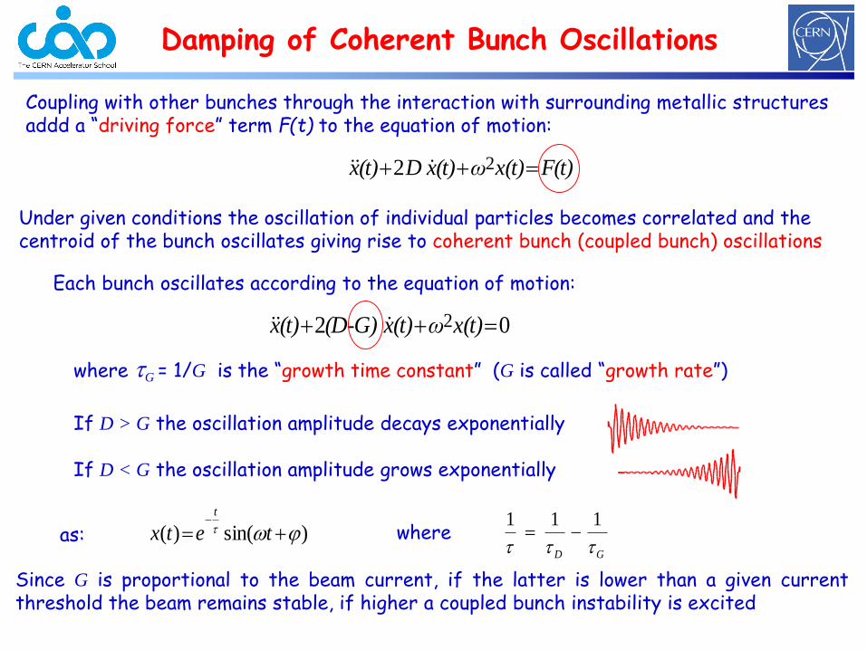
02 2 x(t)ω(t)x(D-G) (t)x

Each bunch oscillates according to the equation of motion:

If D > G the oscillation amplitude decays exponentially

If D < G the oscillation amplitude grows exponentially

F(t)x(t)ω(t)xD (t)x 22

Coupling with other bunches through the interaction with surrounding metallic structures addd a “driving force” term F(t) to the equation of motion:

GD

111

where G = 1/G is the “growth time constant” (G is called “growth rate”)

)sin()(

tetx

t

where

Since G is proportional to the beam current, if the latter is lower than a given currentthreshold the beam remains stable, if higher a coupled bunch instability is excited

as:

Damping of Coherent Bunch Oscillations

Under given conditions the oscillation of individual particles becomes correlated and the centroid of the bunch oscillates giving rise to coherent bunch (coupled bunch) oscillations

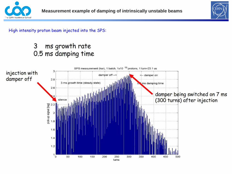
Measurement example of damping of intrinsically unstable beams

High intensity proton beam injected into the SPS:

The feedback action adds a damping term Dfb to the equation of motion

02 2 x(t)ω(t)x) D(D-G(t)xfb

In order to introduce damping, the feedback must provide a kick proportional to the derivative of the bunch oscillation

A multi-bunch feedback detects an instability by means of one or more Beam Position Monitors (BPM) and acts back on the beam by applying electromagnetic ‘kicks’ to the bunches

Since the oscillation is sinusoidal, the kick signal for each bunch can be generated by

shifting by π/2 the oscillation signal of the same bunch when it passes through the kicker

Such that D-G+Dfb > 0

Feedback Damping Action

DETECTOR

PROCESSING

KICKER

H.Schmickler, CERN 15

x

Applied kicks

Position measurements

X’

Illustration of Damping process in phase space

Multi-bunch modes

Typically, betatron tune frequencies (horizontal and vertical) are higher than therevolution frequency, while the synchrotron tune frequency (longitudinal) is lower thanthe revolution frequency

Although each bunch oscillates at the tune frequency, there can be different modesof oscillation, called multi-bunch modes depending on how each bunch oscillates withrespect to the other bunches

0 1 2 3 4Machine Turns

Ex.

Vertical

Tune = 2.25

Longitudinal

Tune = 0.5

Multi-bunch modes

Let us consider M bunches equally spaced around the ring

Each multi-bunch mode is characterized by a bunch-to-bunch phase difference of:

m = multi-bunch mode number (0, 1, .., M-1)M

m2

Each multi-bunch mode is associated to a characteristic set of frequencies:

00 )( n mMp

Where:

p is and integer number - < p <

0 is the revolution frequency

M0 = rf is the RF frequency (bunch repetition frequency)

n is the tune

Two sidebands at ±(m+n)0 for each multiple of the RF frequency

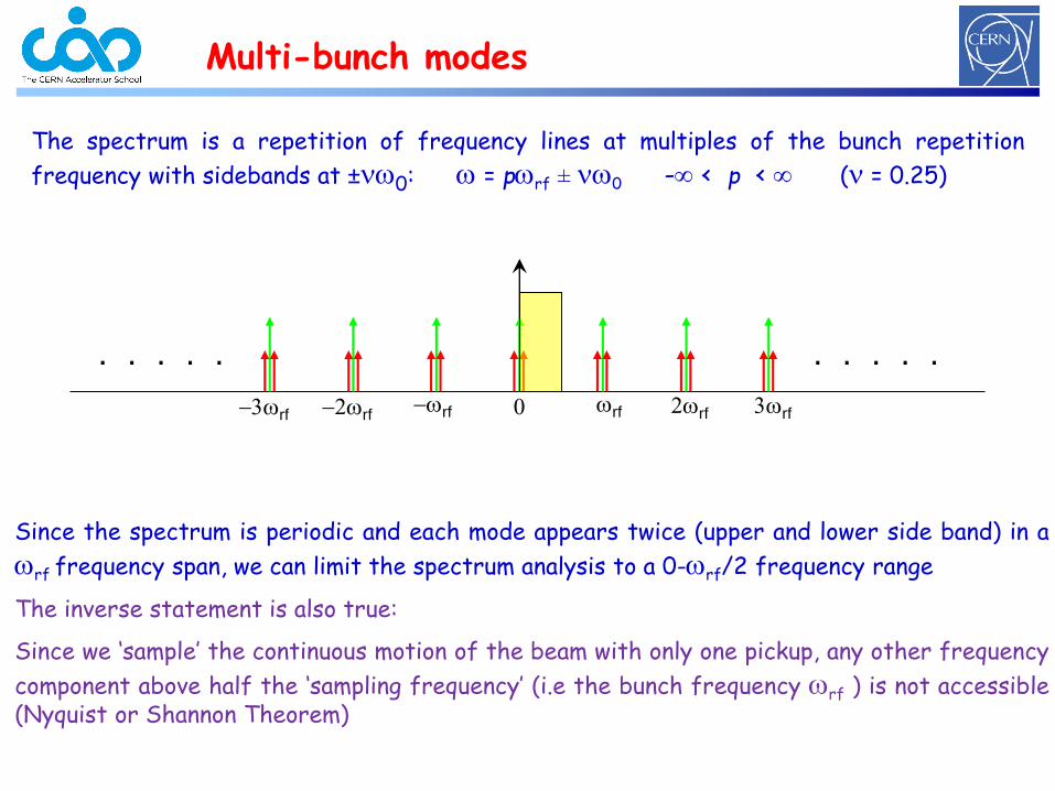
Multi-bunch modes

The spectrum is a repetition of frequency lines at multiples of the bunch repetition

frequency with sidebands at ±n0: = prf ± n0 - < p < (n = 0.25)

Since the spectrum is periodic and each mode appears twice (upper and lower side band) in a

rf frequency span, we can limit the spectrum analysis to a 0-rf/2 frequency range

The inverse statement is also true:

Since we ‘sample’ the continuous motion of the beam with only one pickup, any other frequency

component above half the ‘sampling frequency’ (i.e the bunch frequency rf ) is not accessible(Nyquist or Shannon Theorem)

2rf3rf 0

. . . . . . . . . .

rf 2rf 3rfrf

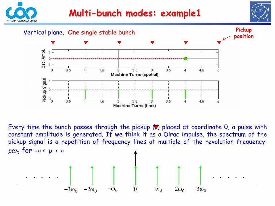
Multi-bunch modes: example1

Vertical plane. One single stable bunch

Every time the bunch passes through the pickup ( ) placed at coordinate 0, a pulse withconstant amplitude is generated. If we think it as a Dirac impulse, the spectrum of thepickup signal is a repetition of frequency lines at multiple of the revolution frequency:

p0 for - < p <

0 20 30

. . . . . . . . . .

02030 0

Pickup position

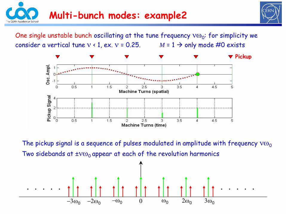
Multi-bunch modes: example2

One single unstable bunch oscillating at the tune frequency n0: for simplicity we

consider a vertical tune n < 1, ex. n = 0.25. M = 1 only mode #0 exists

The pickup signal is a sequence of pulses modulated in amplitude with frequency n0

Two sidebands at ±n0 appear at each of the revolution harmonics

0 20 30

. . . . . . . . . .

02030 0

Pickup

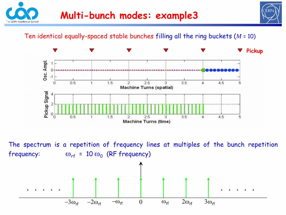
Multi-bunch modes: example3

Ten identical equally-spaced stable bunches filling all the ring buckets (M = 10)

The spectrum is a repetition of frequency lines at multiples of the bunch repetition

frequency: rf = 10 0 (RF frequency)

. . . . . . . . . .

rf 2rf 3rfrf2rf3rf 0

Pickup

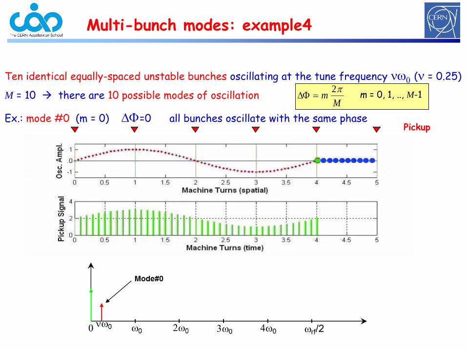
Multi-bunch modes: example4

Ten identical equally-spaced unstable bunches oscillating at the tune frequency n0 (n = 0.25)

M = 10 there are 10 possible modes of oscillation

Ex.: mode #0 (m = 0) =0 all bunches oscillate with the same phase

Mm

2

Pickup

m = 0, 1, .., M-1

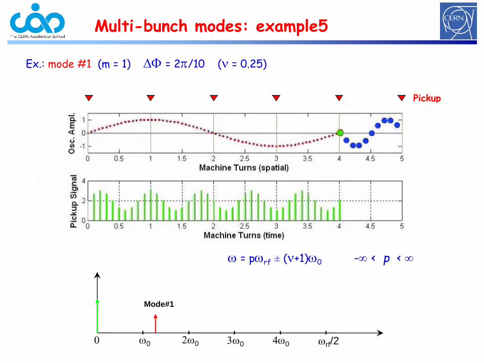
Multi-bunch modes: example5

Ex.: mode #1 (m = 1) = 2/10 (n = 0.25)

= prf ± (n+1)0 - < p <

rf/20 0 20 40

Mode#1

30

Pickup

rf/20 0 20 40

Mode#2

30

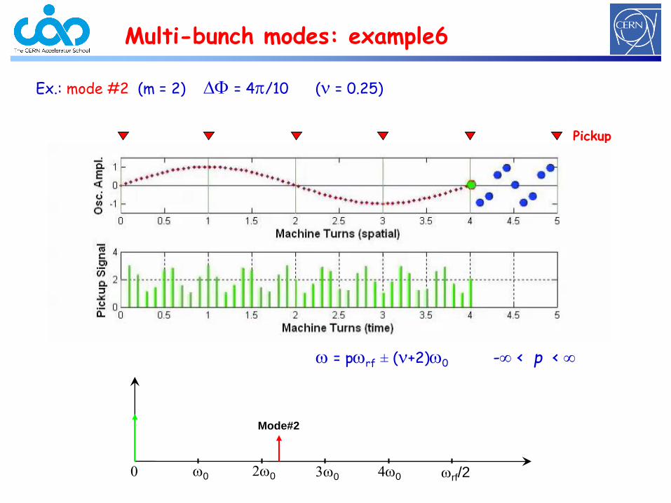
Multi-bunch modes: example6

Ex.: mode #2 (m = 2) = 4/10 (n = 0.25)

= prf ± (n+2)0 - < p <

Pickup

rf/20 0 20 40

Mode#3

30

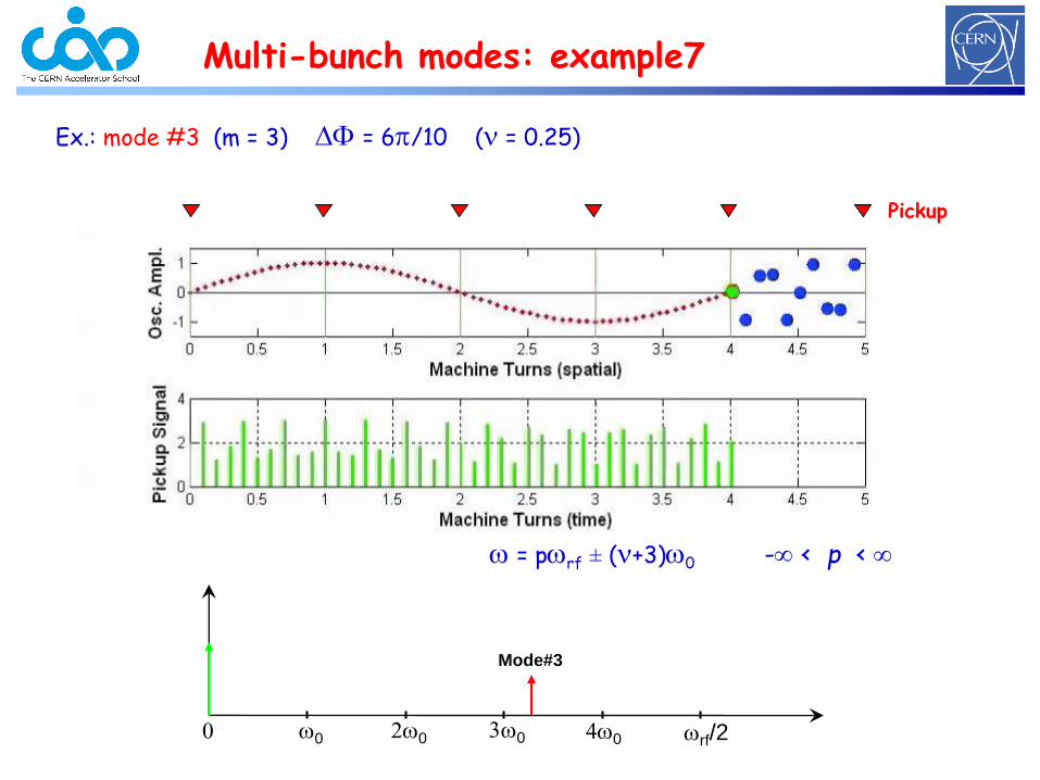
Multi-bunch modes: example7

Ex.: mode #3 (m = 3) = 6/10 (n = 0.25)

= prf ± (n+3)0 - < p <

Pickup

rf/20 0 20 40

Mode#4

30

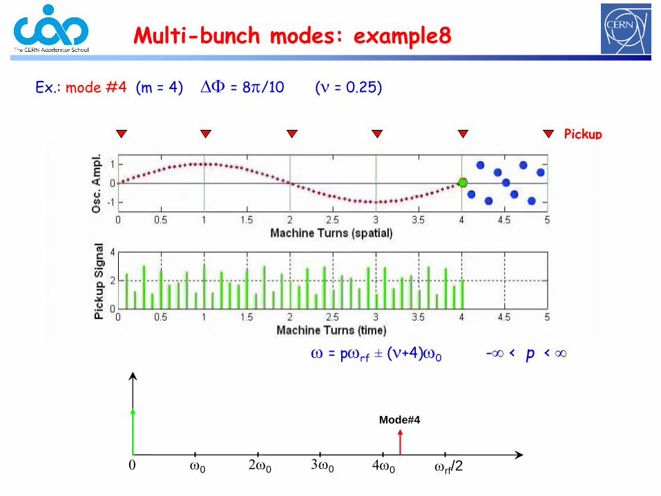
Multi-bunch modes: example8

Ex.: mode #4 (m = 4) = 8/10 (n = 0.25)

= prf ± (n+4)0 - < p <

Pickup

rf/20 0 20 40

Mode#5

30

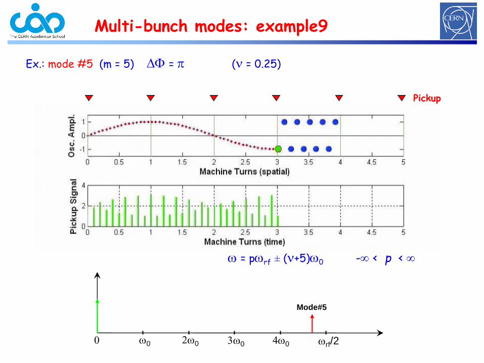
Multi-bunch modes: example9

Ex.: mode #5 (m = 5) = (n = 0.25)

= prf ± (n+5)0 - < p <

Pickup

rf/20 0 20 40

Mode#6

30

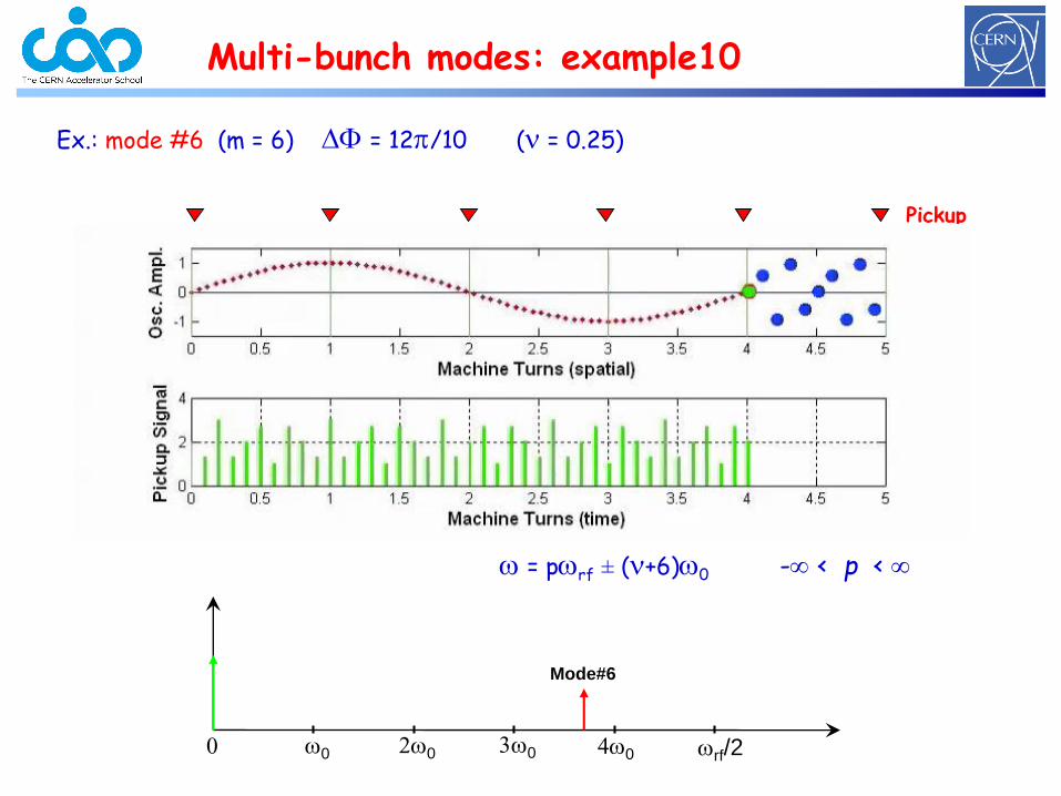
Multi-bunch modes: example10

Ex.: mode #6 (m = 6) = 12/10 (n = 0.25)

= prf ± (n+6)0 - < p <

Pickup

rf/20 0 20 40

Mode#7

30

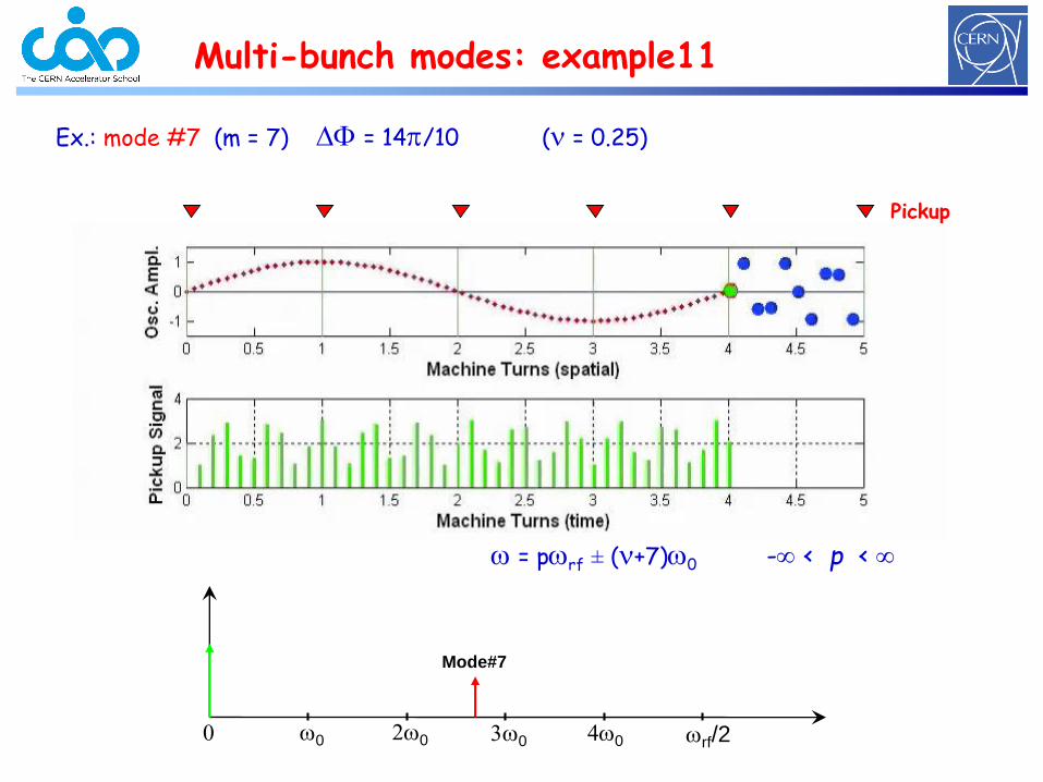
Multi-bunch modes: example11

Ex.: mode #7 (m = 7) = 14/10 (n = 0.25)

= prf ± (n+7)0 - < p <

Pickup

rf/20 0 20 40

Mode#8

30

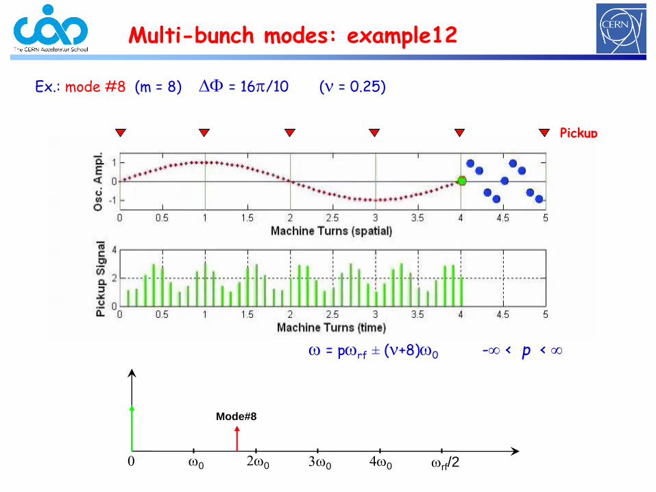
Multi-bunch modes: example12

Ex.: mode #8 (m = 8) = 16/10 (n = 0.25)

= prf ± (n+8)0 - < p <

Pickup

rf/20 0 20 40

Mode#9

30

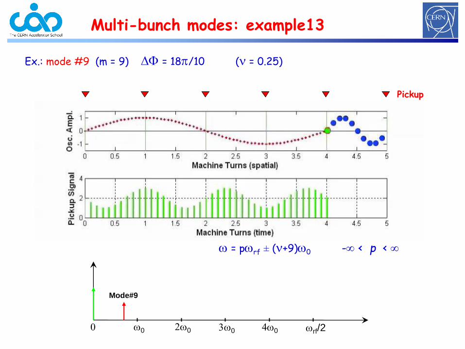
Multi-bunch modes: example13

Ex.: mode #9 (m = 9) = 18/10 (n = 0.25)

= prf ± (n+9)0 - < p <

Pickup

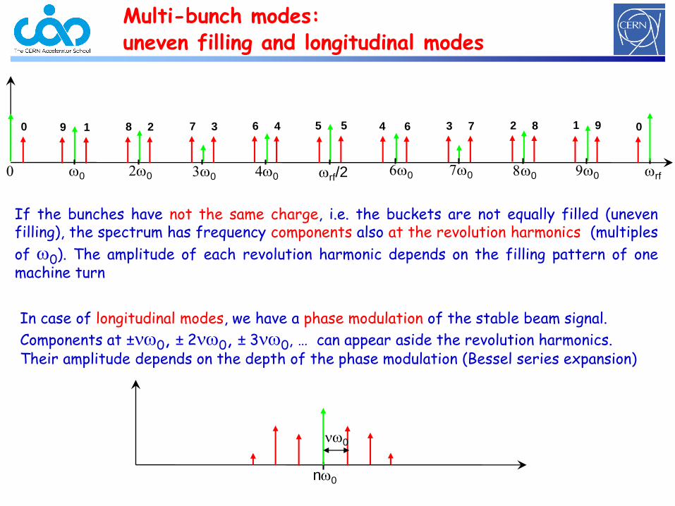
Multi-bunch modes: uneven filling and longitudinal modes

If the bunches have not the same charge, i.e. the buckets are not equally filled (unevenfilling), the spectrum has frequency components also at the revolution harmonics (multiples

of 0). The amplitude of each revolution harmonic depends on the filling pattern of onemachine turn

rf/20 0 20 40

9

30

8 7 6 51 2 3 40

rf60 70 90

4

80

3 2 1 06 7 8 95

In case of longitudinal modes, we have a phase modulation of the stable beam signal.

Components at ±n0, ± 2n0, ± 3n0, … can appear aside the revolution harmonics. Their amplitude depends on the depth of the phase modulation (Bessel series expansion)

n0

n0

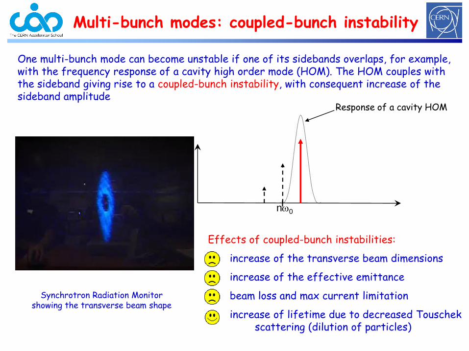
Multi-bunch modes: coupled-bunch instability

One multi-bunch mode can become unstable if one of its sidebands overlaps, for example, with the frequency response of a cavity high order mode (HOM). The HOM couples with the sideband giving rise to a coupled-bunch instability, with consequent increase of the sideband amplitude

n0

Response of a cavity HOM

Effects of coupled-bunch instabilities:

increase of the transverse beam dimensions

increase of the effective emittance

beam loss and max current limitation

increase of lifetime due to decreased Touschek scattering (dilution of particles)

Synchrotron Radiation Monitor showing the transverse beam shape

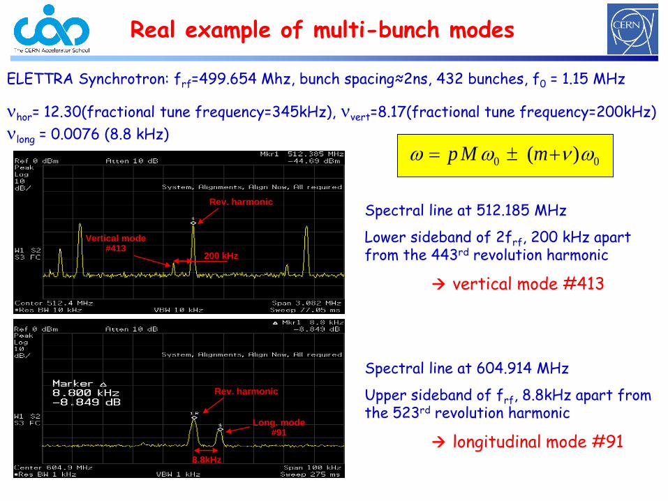
ELETTRA Synchrotron: frf=499.654 Mhz, bunch spacing≈2ns, 432 bunches, f0 = 1.15 MHz

nhor= 12.30(fractional tune frequency=345kHz), nvert=8.17(fractional tune frequency=200kHz)

nlong = 0.0076 (8.8 kHz)

00 )( n mMp

Spectral line at 512.185 MHz

Lower sideband of 2frf, 200 kHz apart from the 443rd revolution harmonic

vertical mode #413

200 kHz

Rev. harmonic

Vertical mode #413

Spectral line at 604.914 MHz

Upper sideband of frf, 8.8kHz apart from the 523rd revolution harmonic

longitudinal mode #91

Rev. harmonic

Long. mode #91

8.8kHz

Real example of multi-bunch modes

Feedback systems

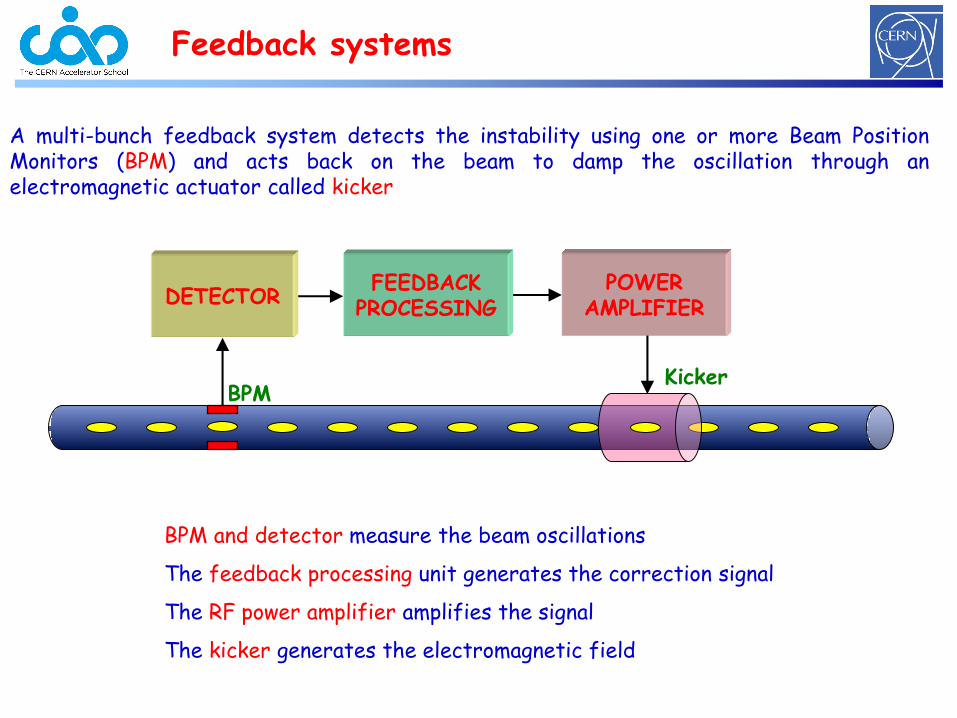
A multi-bunch feedback system detects the instability using one or more Beam PositionMonitors (BPM) and acts back on the beam to damp the oscillation through anelectromagnetic actuator called kicker

DETECTORFEEDBACK

PROCESSINGPOWER

AMPLIFIER

BPMKicker

BPM and detector measure the beam oscillations

The feedback processing unit generates the correction signal

The RF power amplifier amplifies the signal

The kicker generates the electromagnetic field

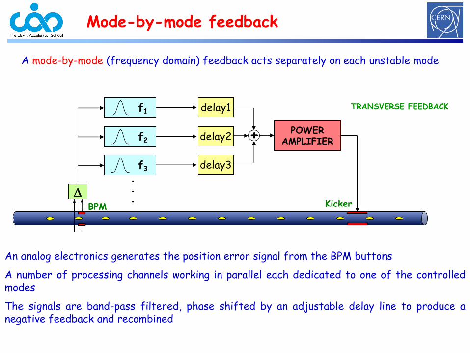
Mode-by-mode feedback

A mode-by-mode (frequency domain) feedback acts separately on each unstable mode

POWERAMPLIFIER

An analog electronics generates the position error signal from the BPM buttons

A number of processing channels working in parallel each dedicated to one of the controlledmodes

The signals are band-pass filtered, phase shifted by an adjustable delay line to produce anegative feedback and recombined

f3 delay3

+f2 delay2

f1 delay1

.

.

.BPM Kicker

TRANSVERSE FEEDBACK

Bunch-by-bunch feedback

A bunch-by-bunch (time domain) feedback individually steers each bunch by applying smallelectromagnetic kicks every time the bunch passes through the kicker: the result is a dampedoscillation lasting several turns

The correction signal for a given bunch is generated based on the motion of the same bunch

POWERAMPLIFIER

Channel1

.

.

.BPM

Channel2

Channel3

Kicker

TRANSVERSE FEEDBACK

delay

Damping the oscillation of each bunch is equivalent to damping all multi-bunch modes

Example of implementation using a time division scheme

Every bunch is measured and corrected at every machine turn but, due to the delay of thefeedback chain, the correction kick corresponding to a given measurement is applied to thebunch one or more turns later

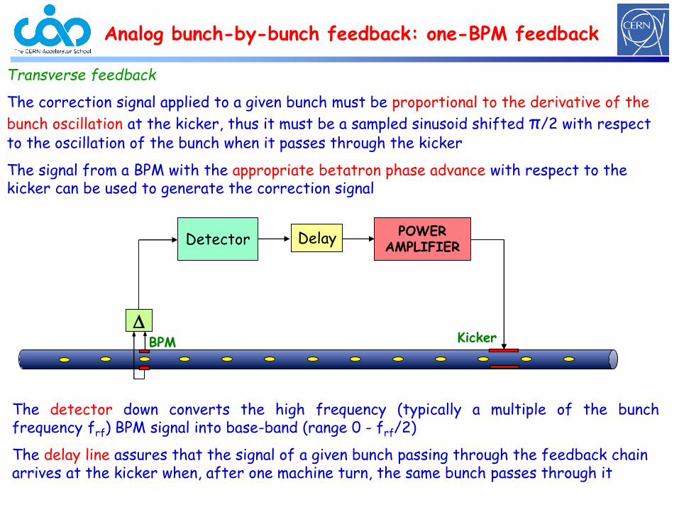
Analog bunch-by-bunch feedback: one-BPM feedback

POWERAMPLIFIER

BPM

Transverse feedback

The correction signal applied to a given bunch must be proportional to the derivative of the

bunch oscillation at the kicker, thus it must be a sampled sinusoid shifted π/2 with respect to the oscillation of the bunch when it passes through the kicker

The signal from a BPM with the appropriate betatron phase advance with respect to the kicker can be used to generate the correction signal

DelayDetector

The detector down converts the high frequency (typically a multiple of the bunchfrequency frf) BPM signal into base-band (range 0 - frf/2)

The delay line assures that the signal of a given bunch passing through the feedback chain arrives at the kicker when, after one machine turn, the same bunch passes through it

Kicker

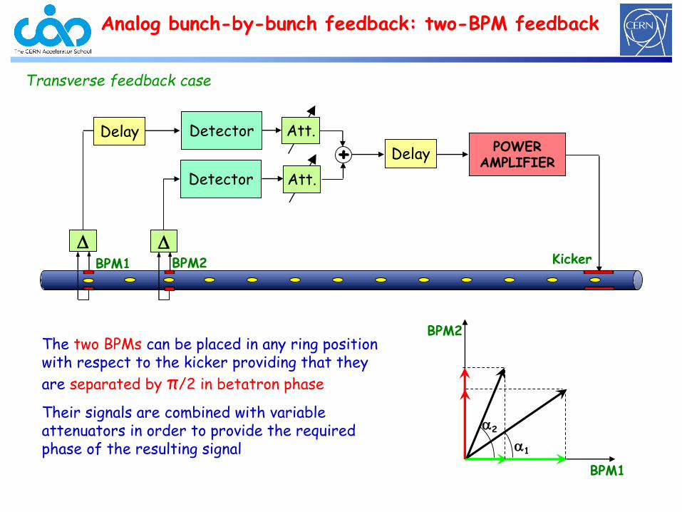
Analog bunch-by-bunch feedback: two-BPM feedback

POWERAMPLIFIER

BPM2

Delay

Detector

Detector

BPM1

+Att.

Att.

Delay

Kicker

The two BPMs can be placed in any ring position with respect to the kicker providing that they

are separated by π/2 in betatron phase

Their signals are combined with variable attenuators in order to provide the required phase of the resulting signal a1

a2

BPM1

BPM2

Transverse feedback case

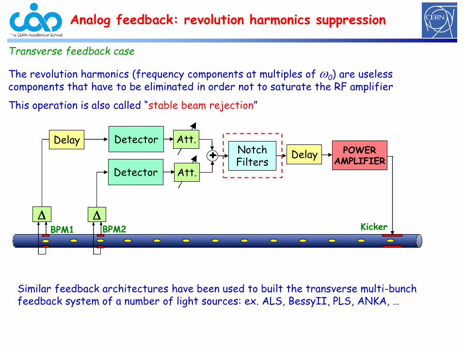
Analog feedback: revolution harmonics suppression

POWERAMPLIFIER

BPM2

Delay

Detector

Detector

BPM1

+Att.

Att.

Transverse feedback case

The revolution harmonics (frequency components at multiples of 0) are useless components that have to be eliminated in order not to saturate the RF amplifier

This operation is also called “stable beam rejection”

Delay

Similar feedback architectures have been used to built the transverse multi-bunch feedback system of a number of light sources: ex. ALS, BessyII, PLS, ANKA, …

NotchFilters

Kicker

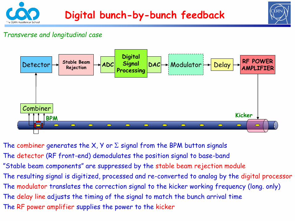
Digital bunch-by-bunch feedback

Transverse and longitudinal case

The combiner generates the X, Y or S signal from the BPM button signals

The detector (RF front-end) demodulates the position signal to base-band

”Stable beam components” are suppressed by the stable beam rejection module

The resulting signal is digitized, processed and re-converted to analog by the digital processor

The modulator translates the correction signal to the kicker working frequency (long. only)

The delay line adjusts the timing of the signal to match the bunch arrival time

The RF power amplifier supplies the power to the kicker

RF POWERAMPLIFIER

Kicker

Detector

Combiner

BPM

ADC

DigitalSignal

ProcessingDACStable Beam

Rejection DelayModulator

42

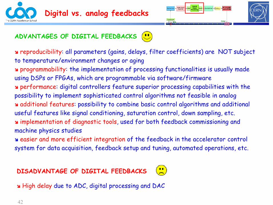
Digital vs. analog feedbacks

ADVANTAGES OF DIGITAL FEEDBACKS

reproducibility: all parameters (gains, delays, filter coefficients) are NOT subject

to temperature/environment changes or aging

programmability: the implementation of processing functionalities is usually made

using DSPs or FPGAs, which are programmable via software/firmware

performance: digital controllers feature superior processing capabilities with the

possibility to implement sophisticated control algorithms not feasible in analog

additional features: possibility to combine basic control algorithms and additional

useful features like signal conditioning, saturation control, down sampling, etc.

implementation of diagnostic tools, used for both feedback commissioning and

machine physics studies

easier and more efficient integration of the feedback in the accelerator control

system for data acquisition, feedback setup and tuning, automated operations, etc.

DISADVANTAGE OF DIGITAL FEEDBACKS

High delay due to ADC, digital processing and DAC

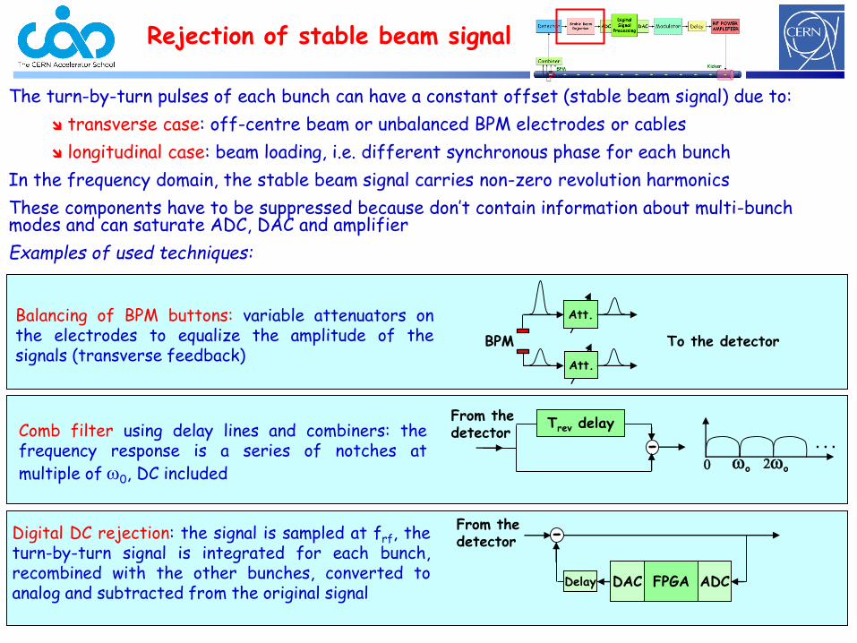
Rejection of stable beam signal

The turn-by-turn pulses of each bunch can have a constant offset (stable beam signal) due to:

transverse case: off-centre beam or unbalanced BPM electrodes or cables

longitudinal case: beam loading, i.e. different synchronous phase for each bunch

In the frequency domain, the stable beam signal carries non-zero revolution harmonics

These components have to be suppressed because don’t contain information about multi-bunch modes and can saturate ADC, DAC and amplifier

Examples of used techniques:

Trev delay

- . . .

o 2o0

From the detectorComb filter using delay lines and combiners: the

frequency response is a series of notches at

multiple of 0, DC included

Att.

Att.

BPM To the detector

Balancing of BPM buttons: variable attenuators onthe electrodes to equalize the amplitude of thesignals (transverse feedback)

Digital DC rejection: the signal is sampled at frf, theturn-by-turn signal is integrated for each bunch,recombined with the other bunches, converted toanalog and subtracted from the original signal

FPGA ADCDAC

-From the detector

Delay

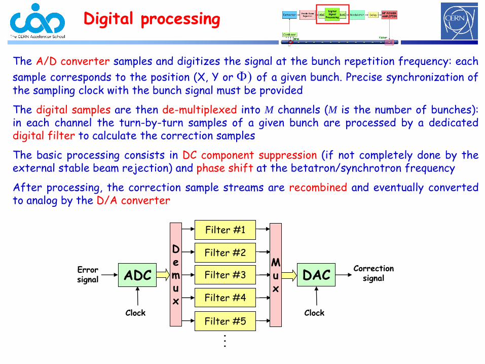
Digital processing

The A/D converter samples and digitizes the signal at the bunch repetition frequency: each

sample corresponds to the position (X, Y or ) of a given bunch. Precise synchronization ofthe sampling clock with the bunch signal must be provided

The digital samples are then de-multiplexed into M channels (M is the number of bunches):in each channel the turn-by-turn samples of a given bunch are processed by a dedicateddigital filter to calculate the correction samples

The basic processing consists in DC component suppression (if not completely done by theexternal stable beam rejection) and phase shift at the betatron/synchrotron frequency

After processing, the correction sample streams are recombined and eventually convertedto analog by the D/A converter

ADC

Filter #1

DACError signal

Clock Clock

Filter #2

Filter #3

Filter #4

Filter #5...

Correction signal

Demux

Mux

45

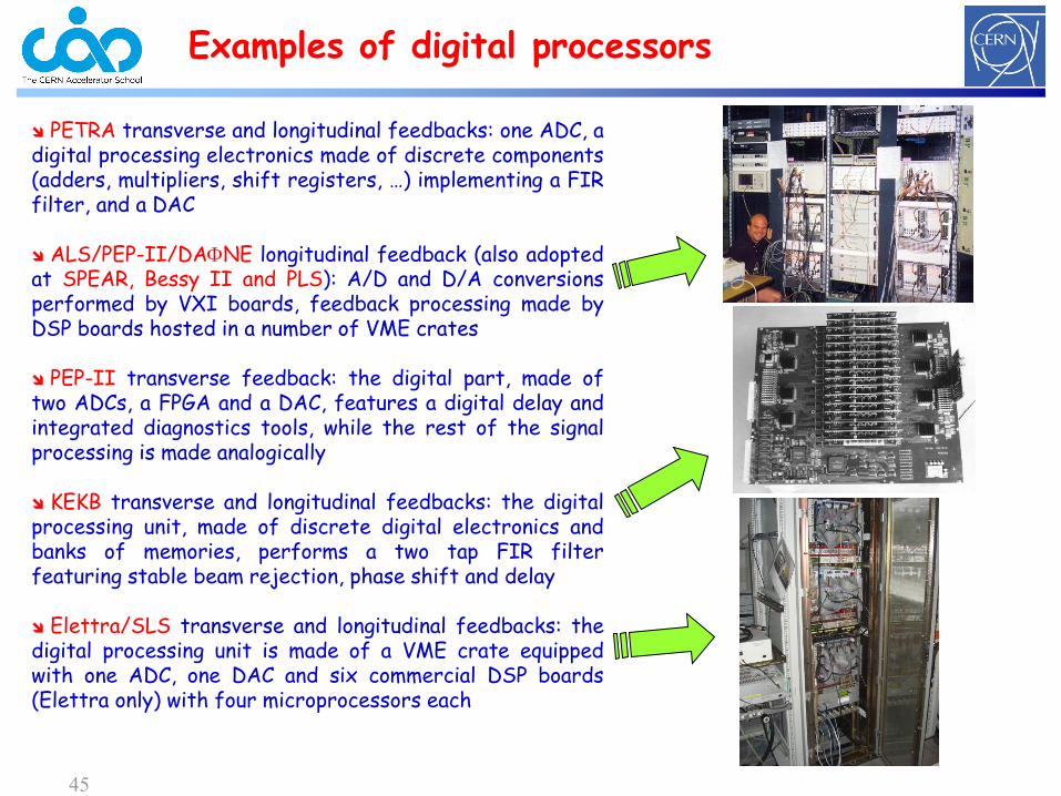
Examples of digital processors

PETRA transverse and longitudinal feedbacks: one ADC, adigital processing electronics made of discrete components(adders, multipliers, shift registers, …) implementing a FIRfilter, and a DAC

ALS/PEP-II/DANE longitudinal feedback (also adoptedat SPEAR, Bessy II and PLS): A/D and D/A conversionsperformed by VXI boards, feedback processing made byDSP boards hosted in a number of VME crates

PEP-II transverse feedback: the digital part, made oftwo ADCs, a FPGA and a DAC, features a digital delay andintegrated diagnostics tools, while the rest of the signalprocessing is made analogically

KEKB transverse and longitudinal feedbacks: the digitalprocessing unit, made of discrete digital electronics andbanks of memories, performs a two tap FIR filterfeaturing stable beam rejection, phase shift and delay

Elettra/SLS transverse and longitudinal feedbacks: thedigital processing unit is made of a VME crate equippedwith one ADC, one DAC and six commercial DSP boards(Elettra only) with four microprocessors each

46

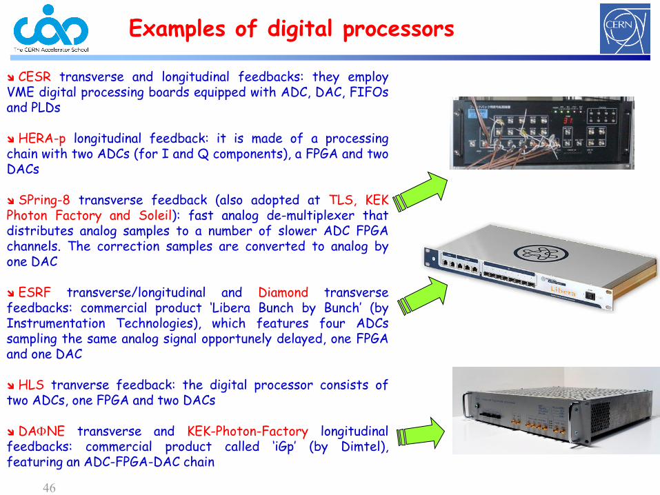
CESR transverse and longitudinal feedbacks: they employVME digital processing boards equipped with ADC, DAC, FIFOsand PLDs

HERA-p longitudinal feedback: it is made of a processingchain with two ADCs (for I and Q components), a FPGA and twoDACs

SPring-8 transverse feedback (also adopted at TLS, KEKPhoton Factory and Soleil): fast analog de-multiplexer thatdistributes analog samples to a number of slower ADC FPGAchannels. The correction samples are converted to analog byone DAC

ESRF transverse/longitudinal and Diamond transversefeedbacks: commercial product ‘Libera Bunch by Bunch’ (byInstrumentation Technologies), which features four ADCssampling the same analog signal opportunely delayed, one FPGAand one DAC

HLS tranverse feedback: the digital processor consists oftwo ADCs, one FPGA and two DACs

DANE transverse and KEK-Photon-Factory longitudinalfeedbacks: commercial product called ‘iGp’ (by Dimtel),featuring an ADC-FPGA-DAC chain

Examples of digital processors

Amplifier and kicker

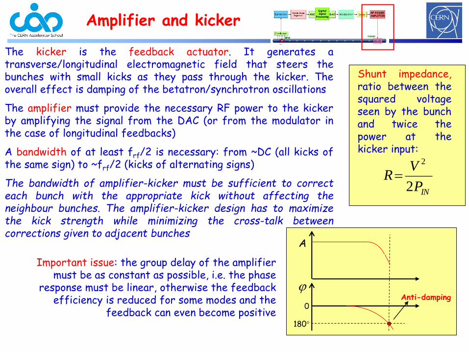
The kicker is the feedback actuator. It generates atransverse/longitudinal electromagnetic field that steers thebunches with small kicks as they pass through the kicker. Theoverall effect is damping of the betatron/synchrotron oscillations

The amplifier must provide the necessary RF power to the kickerby amplifying the signal from the DAC (or from the modulator inthe case of longitudinal feedbacks)

A bandwidth of at least frf/2 is necessary: from ~DC (all kicks ofthe same sign) to ~frf/2 (kicks of alternating signs)

The bandwidth of amplifier-kicker must be sufficient to correcteach bunch with the appropriate kick without affecting theneighbour bunches. The amplifier-kicker design has to maximizethe kick strength while minimizing the cross-talk betweencorrections given to adjacent bunches

INP

VR

2

2

Shunt impedance,ratio between thesquared voltageseen by the bunchand twice thepower at thekicker input:

Important issue: the group delay of the amplifier must be as constant as possible, i.e. the phase

response must be linear, otherwise the feedback efficiency is reduced for some modes and the

feedback can even become positive

A

0

180°

Anti-damping

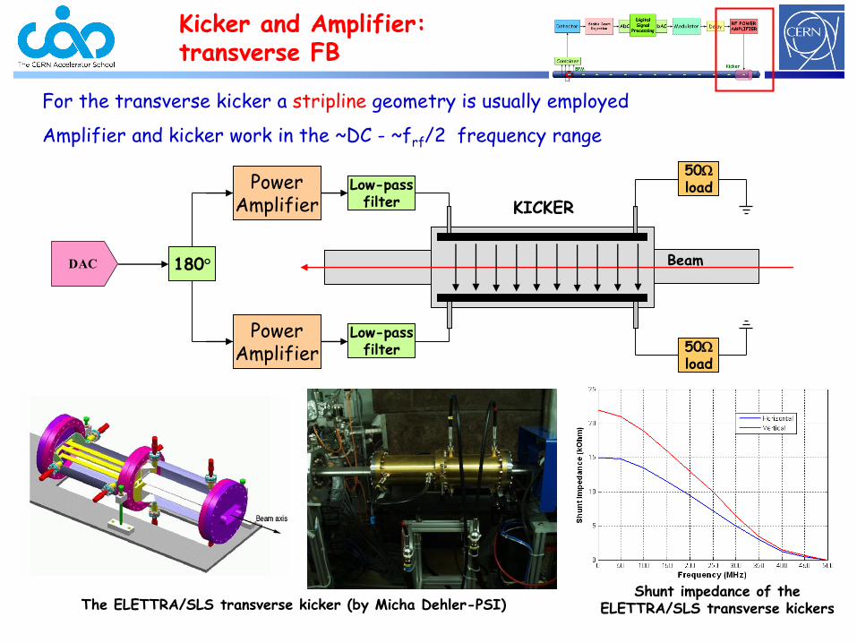
Kicker and Amplifier: transverse FB

For the transverse kicker a stripline geometry is usually employed

Amplifier and kicker work in the ~DC - ~frf/2 frequency range

Beam

PowerAmplifier

50W

load

50W

load

180°

KICKER

DAC

Low-passfilter

PowerAmplifier

Low-passfilter

Shunt impedance of the ELETTRA/SLS transverse kickersThe ELETTRA/SLS transverse kicker (by Micha Dehler-PSI)

Kicker and Amplifier: longitudinal FB

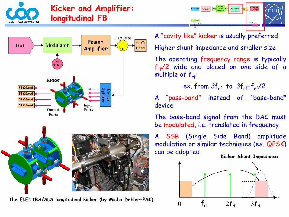
The ELETTRA/SLS longitudinal kicker (by Micha Dehler-PSI)

A “cavity like” kicker is usually preferred

Higher shunt impedance and smaller size

The operating frequency range is typicallyfrf/2 wide and placed on one side of amultiple of frf:

ex. from 3frf to 3frf+frf/2

A “pass-band” instead of “base-band”device

The base-band signal from the DAC mustbe modulated, i.e. translated in frequency

A SSB (Single Side Band) amplitudemodulation or similar techniques (ex. QPSK)can be adopted

frf 2frf 3frf0

Kicker Shunt Impedance

2

max

2

0

2

2

B

BB

KK

K

AT

e

E

RP

Required damping time

Max oscillation amplitude

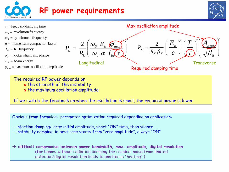
RF power requirements

The required RF power depends on: the strength of the instability the maximum oscillation amplitude

If we switch the feedback on when the oscillation is small, the required power is lower

2

0

max2

a

RF

BS

k

kf

E

RP

amplitudenoscillatiomaximum

energybeam

impedanceshuntkicker

frequencyRF

factorcompactionmomentum

frequencynsynchrotro

frequencyrevolution

timedampingfeedback

max

0

B

k

rf

S

E

R

f

α

ω

ω

τ

Longitudinal Transverse

Obvious from formulae: parameter optimization required depending on application:

- injection damping: large initial amplitude, short “ON” time, then silence- instability damping: in best case starts from “zero amplitude”, always “ON”

difficult compromise between power bandwidth, max. amplitude, digital resolution(for beams without radiation damping the residual noise from limited detector/digital resolution leads to emittance “heating”.)

Digital signal processing

M channel/filters each dedicated to one bunch: M is the number of bunches

To damp the bunch oscillations the turn-by-turn kick signal must be the derivative of the bunch position atthe kicker: for a given oscillation frequency a /2 phase shifted signal must be generated

In determining the real phase shift to perform in each channel, the phase advance between BPM and kickermust be taken into account as well as any additional delay due to the feedback latency (multiple of onemachine revolution period)

The digital processing must also reject any residual constant offset (stable beam component) from thebunch signal to avoid DAC saturation

Digital filters can be implemented with FIR (Finite Impulse Response) or IIR (Infinite Impulse Response)structures. Various techniques are used in the design: ex. frequency domain design and model based design

A filter on the full-rate data stream can compensate for amplifier/kicker not-ideal behaviour

ADC

Filter #1

DACError signal

Filter #2

Filter #3

Filter #4

Filter #5...

Correction signal

Demux

Mux

CompensationFilter

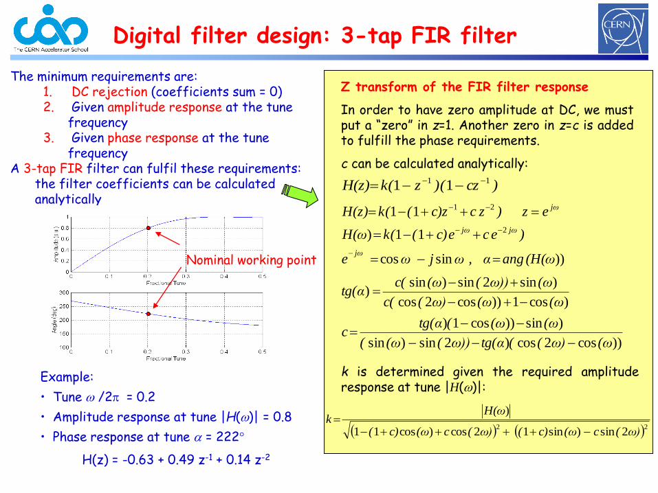
Digital filter design: 3-tap FIR filter

The minimum requirements are:1. DC rejection (coefficients sum = 0)2. Given amplitude response at the tune

frequency3. Given phase response at the tune

frequencyA 3-tap FIR filter can fulfil these requirements:

the filter coefficients can be calculated analytically

Example:

• Tune /2 = 0.2

• Amplitude response at tune |H()| = 0.8

• Phase response at tune a = 222°

H(z) = -0.63 + 0.49 z-1 + 0.14 z-2

Z transform of the FIR filter response

In order to have zero amplitude at DC, we mustput a “zero” in z=1. Another zero in z=c is addedto fulfill the phase requirements.

c can be calculated analytically:

k is determined given the required amplituderesponse at tune |H()|:

Nominal working point

))cos2cos)2sin)sin

)sin))cos1)

)cos1))cos2cos

)sin2sin)sin)

))sincos

11)

11

2

21

(ωω)((tg(αω))((ω(

(ω(ω(tg(αc

(ω(ωω)(c(

(ωω))((ωc(tg(α

(H(ωangα,ωjωe

)ecec)(k(H(ω

ez)zcc)z(k(H(z)

jω

jωjω

jω

)cz()zk(H(z) 11 11

) )222sin)sin12cos)cos11

)

ω)(c(ωc)(ω)(c(ωc)(

H(ωk

H.Schmickler, CERN 53

x

Applied kicks

Position measurements

X’

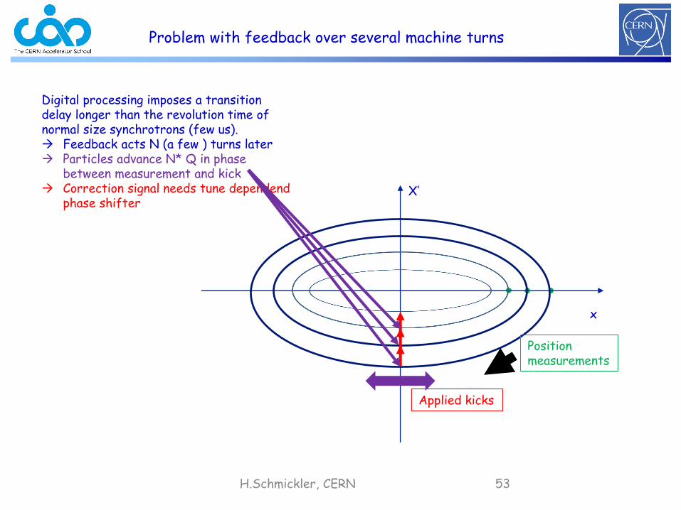
Problem with feedback over several machine turns

Digital processing imposes a transition delay longer than the revolution time of normal size synchrotrons (few us). Feedback acts N (a few ) turns later Particles advance N* Q in phase

between measurement and kick Correction signal needs tune dependend

phase shifter

54

http://www.micromodeler.com/dsp/#

55

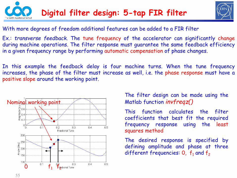
Digital filter design: 5-tap FIR filter

With more degrees of freedom additional features can be added to a FIR filter

Ex.: transverse feedback. The tune frequency of the accelerator can significantly changeduring machine operations. The filter response must guarantee the same feedback efficiencyin a given frequency range by performing automatic compensation of phase changes.

In this example the feedback delay is four machine turns. When the tune frequencyincreases, the phase of the filter must increase as well, i.e. the phase response must have apositive slope around the working point.

The filter design can be made using theMatlab function invfreqz()

This function calculates the filtercoefficients that best fit the requiredfrequency response using the leastsquares method

The desired response is specified bydefining amplitude and phase at threedifferent frequencies: 0, f1 and f2

Nominal working point

f1 f20

56

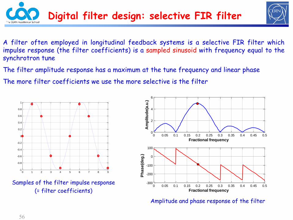
Digital filter design: selective FIR filter

A filter often employed in longitudinal feedback systems is a selective FIR filter whichimpulse response (the filter coefficients) is a sampled sinusoid with frequency equal to thesynchrotron tune

The filter amplitude response has a maximum at the tune frequency and linear phase

The more filter coefficients we use the more selective is the filter

0 0.05 0.1 0.15 0.2 0.25 0.3 0.35 0.4 0.45 0.50

2

4

6

Fractional frequency

Am

plitu

de

(a.u

.)

0 0.05 0.1 0.15 0.2 0.25 0.3 0.35 0.4 0.45 0.5-300

-200

-100

0

100

Fractional frequency

Ph

as

e(d

eg

.)

Samples of the filter impulse response

(= filter coefficients)

0 1 2 3 4 5 6 7 8 9-1

-0.8

-0.6

-0.4

-0.2

0

0.2

0.4

0.6

0.8

1

Amplitude and phase response of the filter

57

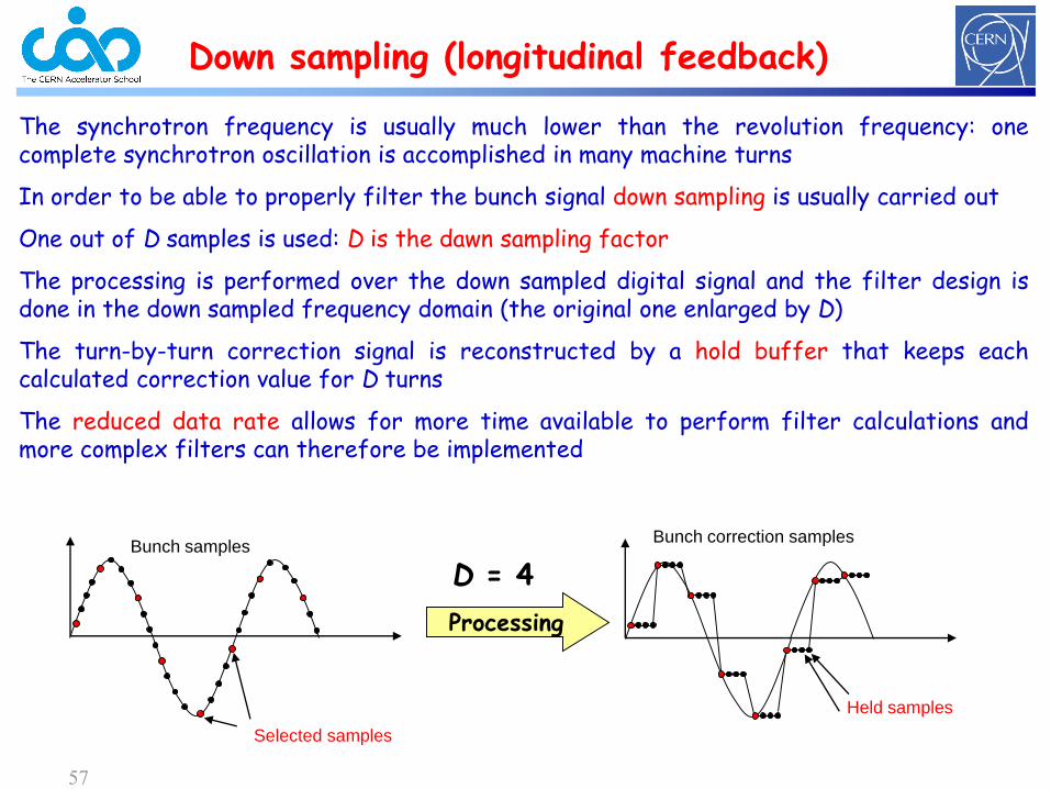
Down sampling (longitudinal feedback)

The synchrotron frequency is usually much lower than the revolution frequency: onecomplete synchrotron oscillation is accomplished in many machine turns

In order to be able to properly filter the bunch signal down sampling is usually carried out

One out of D samples is used: D is the dawn sampling factor

The processing is performed over the down sampled digital signal and the filter design isdone in the down sampled frequency domain (the original one enlarged by D)

The turn-by-turn correction signal is reconstructed by a hold buffer that keeps eachcalculated correction value for D turns

The reduced data rate allows for more time available to perform filter calculations andmore complex filters can therefore be implemented

D = 4Bunch samples

Bunch correction samples

Selected samples

Held samples

Processing

58

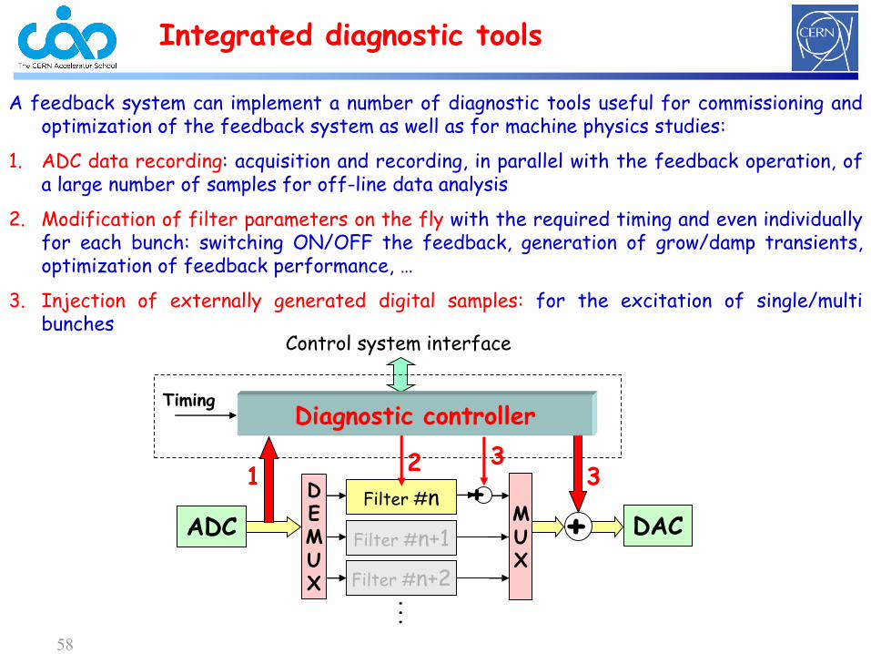
Integrated diagnostic tools

A feedback system can implement a number of diagnostic tools useful for commissioning andoptimization of the feedback system as well as for machine physics studies:

1. ADC data recording: acquisition and recording, in parallel with the feedback operation, ofa large number of samples for off-line data analysis

2. Modification of filter parameters on the fly with the required timing and even individuallyfor each bunch: switching ON/OFF the feedback, generation of grow/damp transients,optimization of feedback performance, …

3. Injection of externally generated digital samples: for the excitation of single/multibunches

ADCFilter #n

DACFilter #n+1

Filter #n+2

DEMUX

MUX

...

Timing

Control system interface

++

12 3

3

Diagnostic controller

59

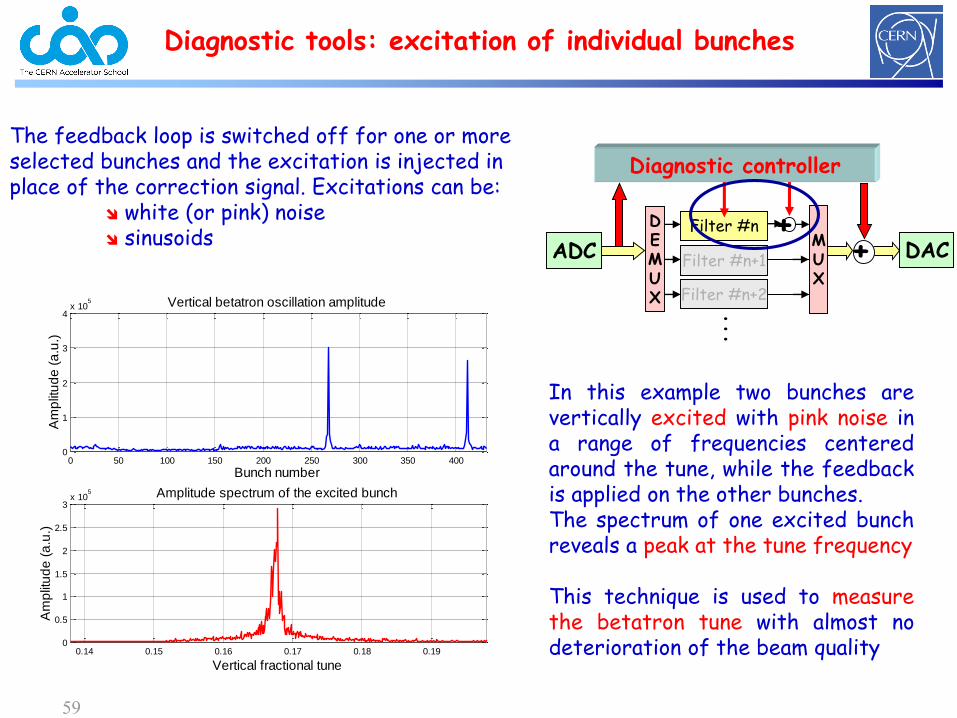
Diagnostic tools: excitation of individual bunches

The feedback loop is switched off for one or more selected bunches and the excitation is injected in place of the correction signal. Excitations can be:

white (or pink) noise sinusoids

0 50 100 150 200 250 300 350 4000

1

2

3

4x 10

5

Bunch number

Am

plit

ud

e (

a.u

.)

Vertical betatron oscillation amplitude

0.14 0.15 0.16 0.17 0.18 0.190

0.5

1

1.5

2

2.5

3x 10

5

Vertical fractional tune

Am

plit

ud

e (

a.u

.)

Amplitude spectrum of the excited bunch

In this example two bunches arevertically excited with pink noise ina range of frequencies centeredaround the tune, while the feedbackis applied on the other bunches.The spectrum of one excited bunchreveals a peak at the tune frequency

This technique is used to measurethe betatron tune with almost nodeterioration of the beam quality

ADCFilter #n

DACFilter #n+1

Filter #n+2

DEMUX

MUX

...

++

Diagnostic controller

60

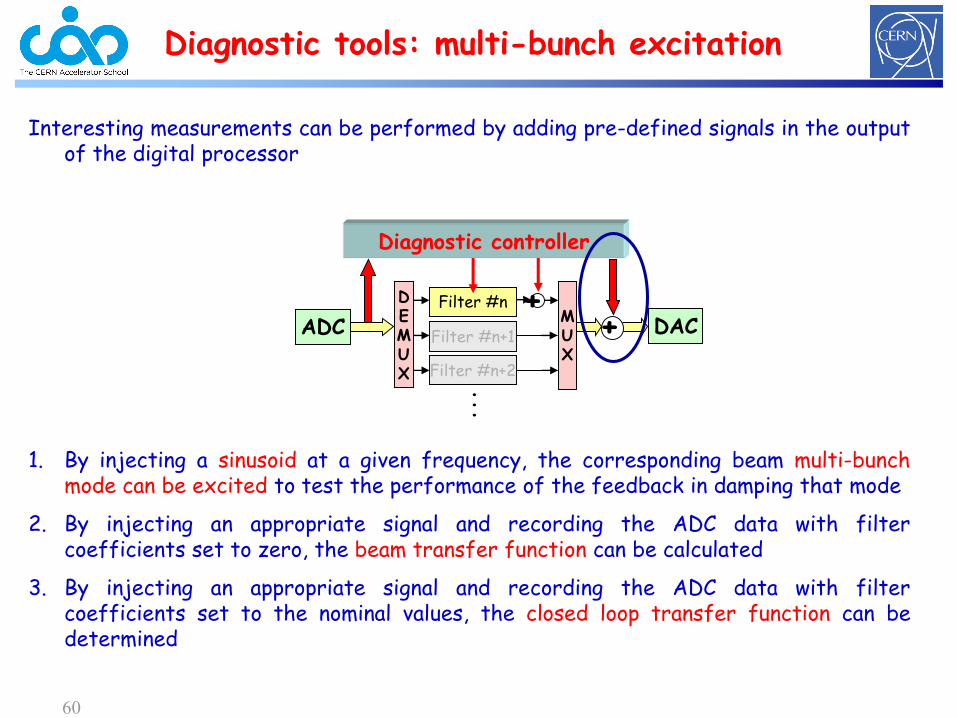
Diagnostic tools: multi-bunch excitation

Interesting measurements can be performed by adding pre-defined signals in the outputof the digital processor

1. By injecting a sinusoid at a given frequency, the corresponding beam multi-bunchmode can be excited to test the performance of the feedback in damping that mode

2. By injecting an appropriate signal and recording the ADC data with filtercoefficients set to zero, the beam transfer function can be calculated

3. By injecting an appropriate signal and recording the ADC data with filtercoefficients set to the nominal values, the closed loop transfer function can bedetermined

ADCFilter #n

DACFilter #n+1

Filter #n+2

DEMUX

MUX

...

++

Diagnostic controller

61

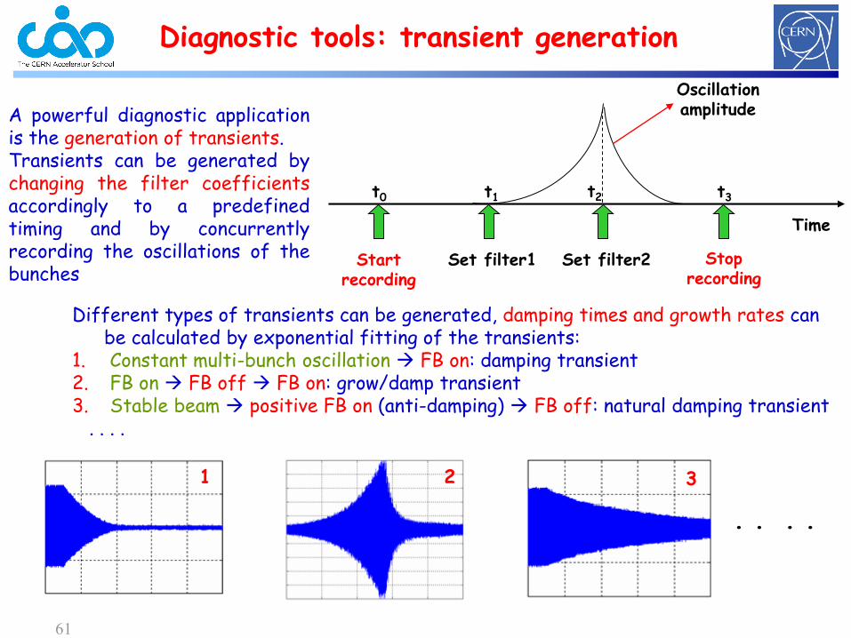
Diagnostic tools: transient generation

Different types of transients can be generated, damping times and growth rates can be calculated by exponential fitting of the transients:

1. Constant multi-bunch oscillation FB on: damping transient2. FB on FB off FB on: grow/damp transient3. Stable beam positive FB on (anti-damping) FB off: natural damping transient

. . . .

A powerful diagnostic applicationis the generation of transients.Transients can be generated bychanging the filter coefficientsaccordingly to a predefinedtiming and by concurrentlyrecording the oscillations of thebunches

Time

Start recording

Set filter1 Set filter2 Stop recording

Oscillation amplitude

1 2

t0 t1 t2 t3

3

. . . .

62

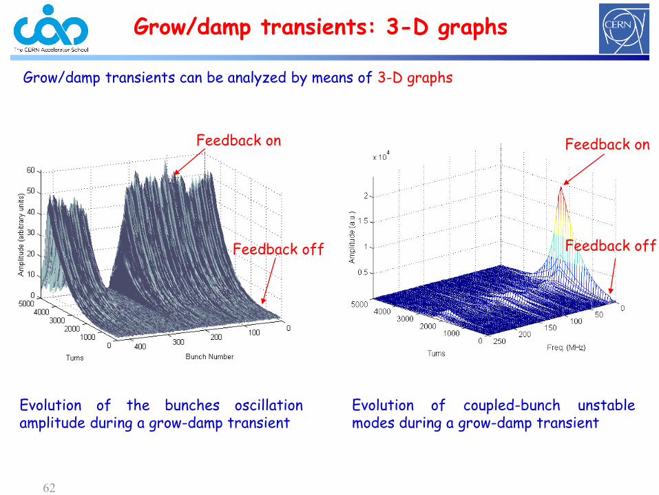
Grow/damp transients can be analyzed by means of 3-D graphs

Grow/damp transients: 3-D graphs

Evolution of coupled-bunch unstablemodes during a grow-damp transient

Feedback on

Feedback off

Feedback on

Feedback off

Evolution of the bunches oscillationamplitude during a grow-damp transient

63

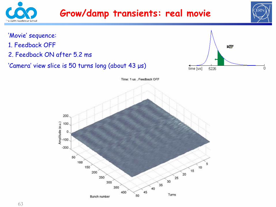
‘Movie’ sequence:

1. Feedback OFF

2. Feedback ON after 5.2 ms

‘Camera’ view slice is 50 turns long (about 43 μs)

Grow/damp transients: real movie

64

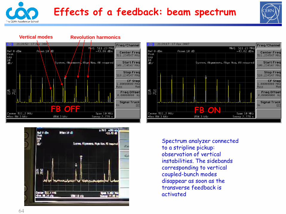
Effects of a feedback: beam spectrum

Revolution harmonicsVertical modes

FB OFF FB ON

Spectrum analyzer connected to a stripline pickup: observation of vertical instabilities. The sidebands corresponding to vertical coupled-bunch modes disappear as soon as the transverse feedback is activated

65

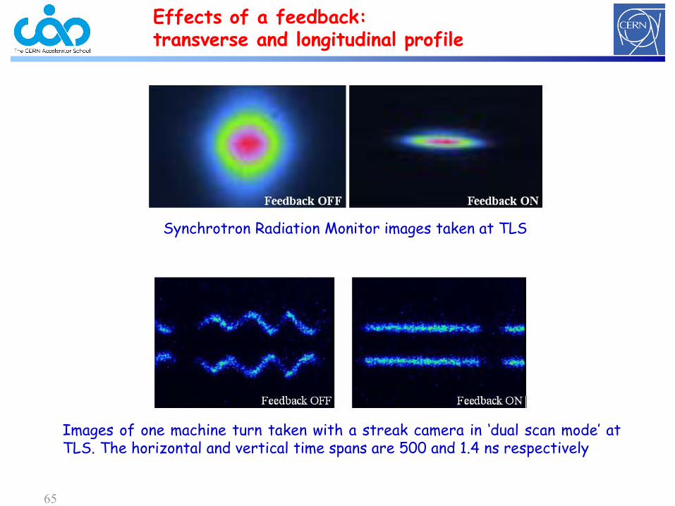
Effects of a feedback: transverse and longitudinal profile

Synchrotron Radiation Monitor images taken at TLS

Images of one machine turn taken with a streak camera in ‘dual scan mode’ atTLS. The horizontal and vertical time spans are 500 and 1.4 ns respectively

66

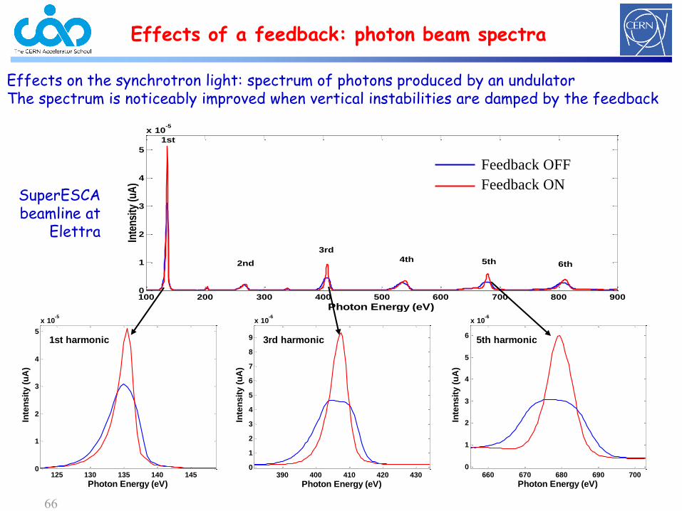
Effects of a feedback: photon beam spectra

Pin-hole camera images at SLS/PSI (courtesy of Micha Dehler)

100 200 300 400 500 600 700 800 9000

1

2

3

4

5

x 10-5

Photon Energy (eV)

Inte

nsi

ty (

uA

)1st

2nd 6th4th 5th

3rd

125 130 135 140 1450

1

2

3

4

5

x 10-5

Photon Energy (eV)

Inte

nsit

y (

uA

)

1st harmonic

390 400 410 420 4300

1

2

3

4

5

6

7

8

9

x 10-6

Photon Energy (eV)

Inte

nsit

y (

uA

)

3rd harmonic

660 670 680 690 7000

1

2

3

4

5

6

x 10-6

Photon Energy (eV)

Inte

nsit

y (

uA

)

5th harmonic

Feedback OFF

Feedback ON

Effects on the synchrotron light: spectrum of photons produced by an undulatorThe spectrum is noticeably improved when vertical instabilities are damped by the feedback

SuperESCA beamline at

Elettra

67

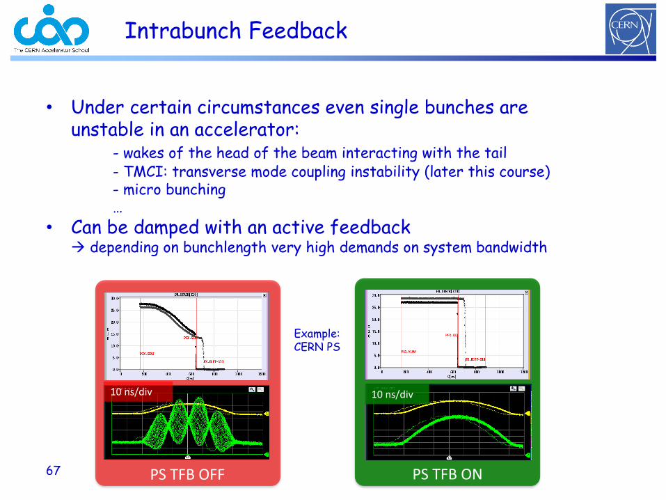
Intrabunch Feedback

• Under certain circumstances even single bunches are unstable in an accelerator:

- wakes of the head of the beam interacting with the tail- TMCI: transverse mode coupling instability (later this course)- micro bunching…

• Can be damped with an active feedback depending on bunchlength very high demands on system bandwidth

10 ns/div

PS TFB OFF

10 ns/div

PS TFB ON

Example: CERN PS

68

Intrabunch Feedback : SPS tests

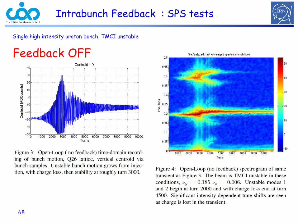
Single high intensity proton bunch, TMCI unstable

Feedback OFF

69

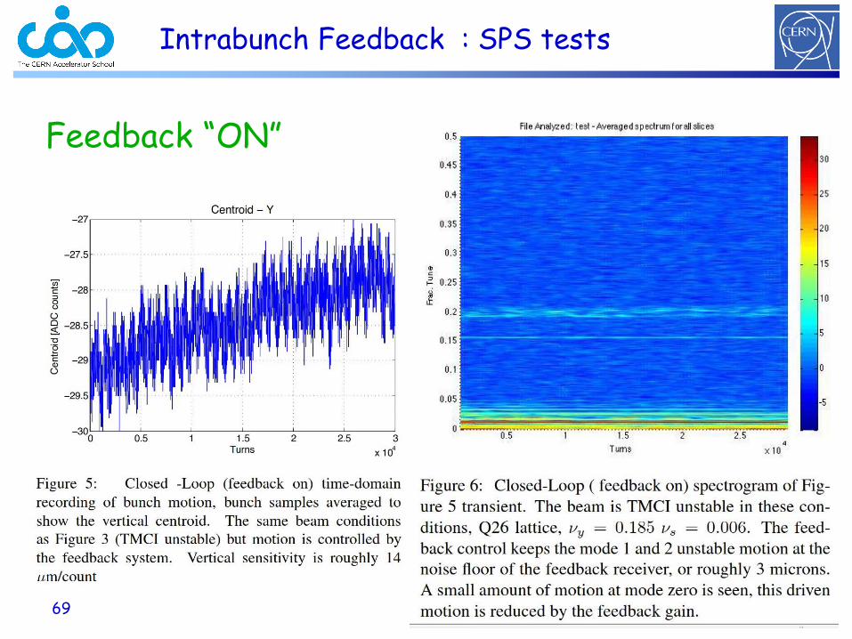
Intrabunch Feedback : SPS tests

Feedback “ON”

70

Injection damping (1/3)

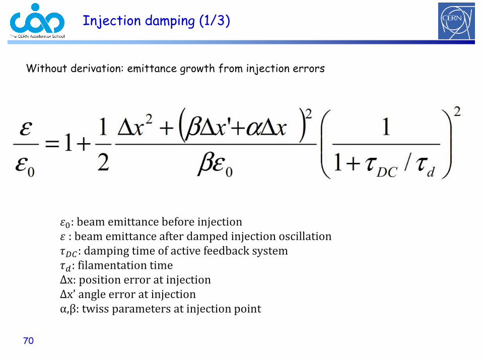
Without derivation: emittance growth from injection errors

𝜀0: beam emittance before injection𝜀 : beam emittance after damped injection oscillation𝜏𝐷𝐶: damping time of active feedback system𝜏𝑑: filamentation timeΔx: position error at injectionΔx’ angle error at injectionα,β: twiss parameters at injection point

71

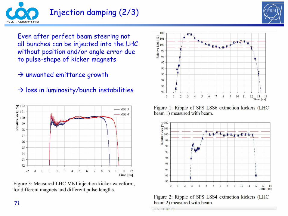
Injection damping (2/3)

Even after perfect beam steering not all bunches can be injected into the LHC without position and/or angle error due to pulse-shape of kicker magnets

unwanted emittance growth

loss in luminosity/bunch instabilities

72

Injection damping (3/3)

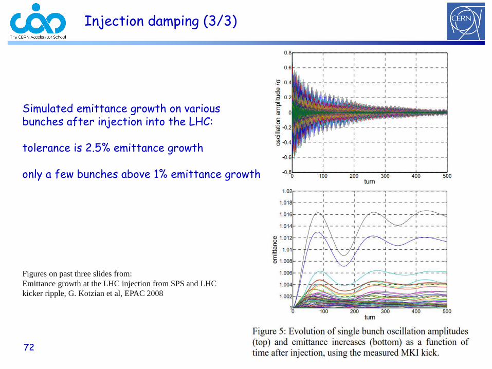
Simulated emittance growth on various bunches after injection into the LHC:

tolerance is 2.5% emittance growth

only a few bunches above 1% emittance growth

Figures on past three slides from:

Emittance growth at the LHC injection from SPS and LHC

kicker ripple, G. Kotzian et al, EPAC 2008

73

References and acknowledges

Marco Lonza (Elletra) for his splendid animations

Many papers about coupled-bunch instabilities and multi-bunch feedbacksystems (PETRA, KEK, SPring-8, Dane, ALS, PEP-II, SPEAR, ESRF, Elettra,SLS, CESR, HERA, HLS, DESY, PLS, BessyII, SRRC, SPS, LHC, …)

Intrabunch feedback at the SPS: Wideband vertical intra-bunch feedback at the SPSJ. Fox (SLAC), W.Hofle (CERN) et al., proceedings of IPAC 2015, Richmond USA

Injection damping: Verena Kain; CAS in Erice 2017

74

Appendix

1. 3 slides : Power requirements for transverse dampers

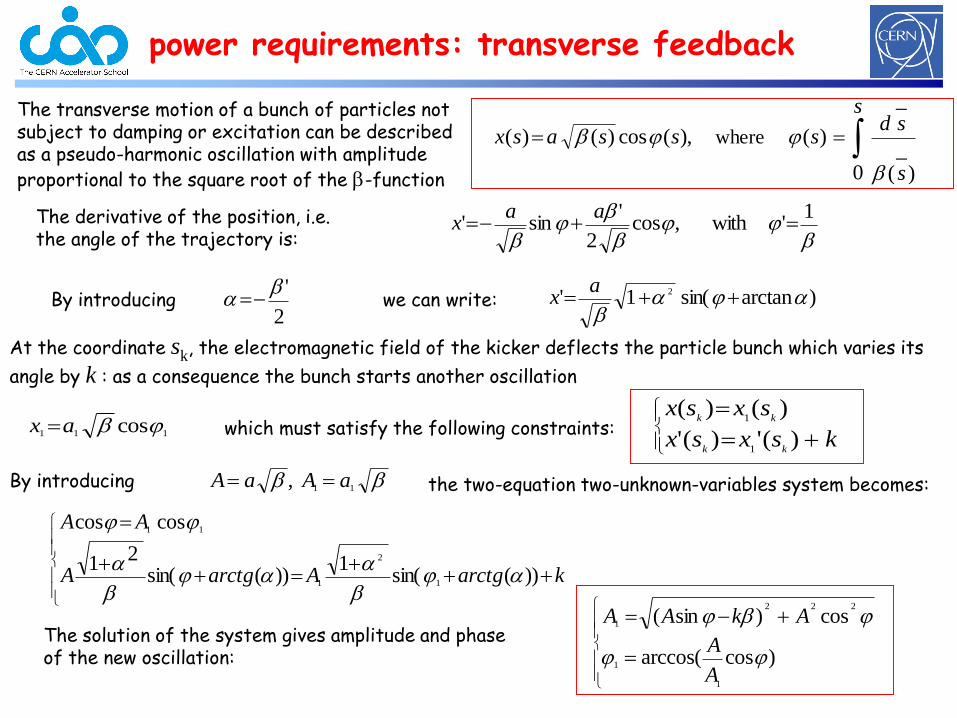
power requirements: transverse feedback

s

s

sdsssasx

0 )_

(

_

)( ),(cos)()( where

1'with ,cos

2

'sin'

aax

2

'a )arctansin(1' 2 aa

ax

The transverse motion of a bunch of particles not subject to damping or excitation can be described as a pseudo-harmonic oscillation with amplitude

proportional to the square root of the -function

The derivative of the position, i.e. the angle of the trajectory is:

By introducing we can write:

111 cosax

ksxsx

sxsx

kk

kk

)(')('

)()(

1

1

At the coordinate sk, the electromagnetic field of the kicker deflects the particle bunch which varies its

angle by k : as a consequence the bunch starts another oscillation

which must satisfy the following constraints:

11, aAaA

karctgAarctgA

AA

))(sin(1

))(sin(21

coscos

1

2

1

11

a

aa

a

By introducing the two-equation two-unknown-variables system becomes:

The solution of the system gives amplitude and phase of the new oscillation:

)cosarccos(

cos)sin(

1

1

222

1

A

A

AkAA

The optimal gain gopt is determined by the maximum kick value kmax that the kicker is able to generate. The

feedback gain must be set so that kmax is generated when the oscillation amplitude A at the kicker location is

maximum:

1 0with sin g β

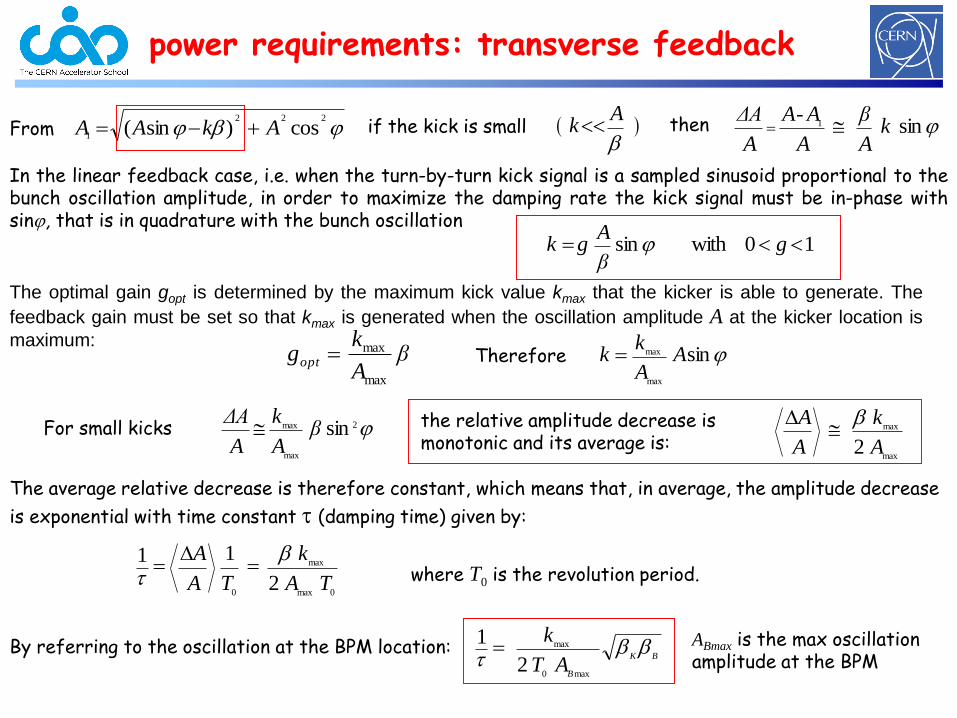
Agk

In the linear feedback case, i.e. when the turn-by-turn kick signal is a sampled sinusoid proportional to thebunch oscillation amplitude, in order to maximize the damping rate the kick signal must be in-phase withsin, that is in quadrature with the bunch oscillation

sin1 kA

β

A

A-A

A

ΔA

max

max

2 A

k

A

A

For small kicks the relative amplitude decrease is

monotonic and its average is:

The average relative decrease is therefore constant, which means that, in average, the amplitude decrease

is exponential with time constant (damping time) given by:

0max

max

02

11

TA

k

TA

A

where T0 is the revolution period.

βA

kgopt

max

max Therefore AA

kk sin

max

max

)

Ak then

2

max

max sinβA

k

A

ΔA

if the kick is small

BK

BAT

k

max0

max

2

1By referring to the oscillation at the BPM location: ABmax is the max oscillation

amplitude at the BPM

222

1 cos)sin( AkAA From

power requirements: transverse feedback

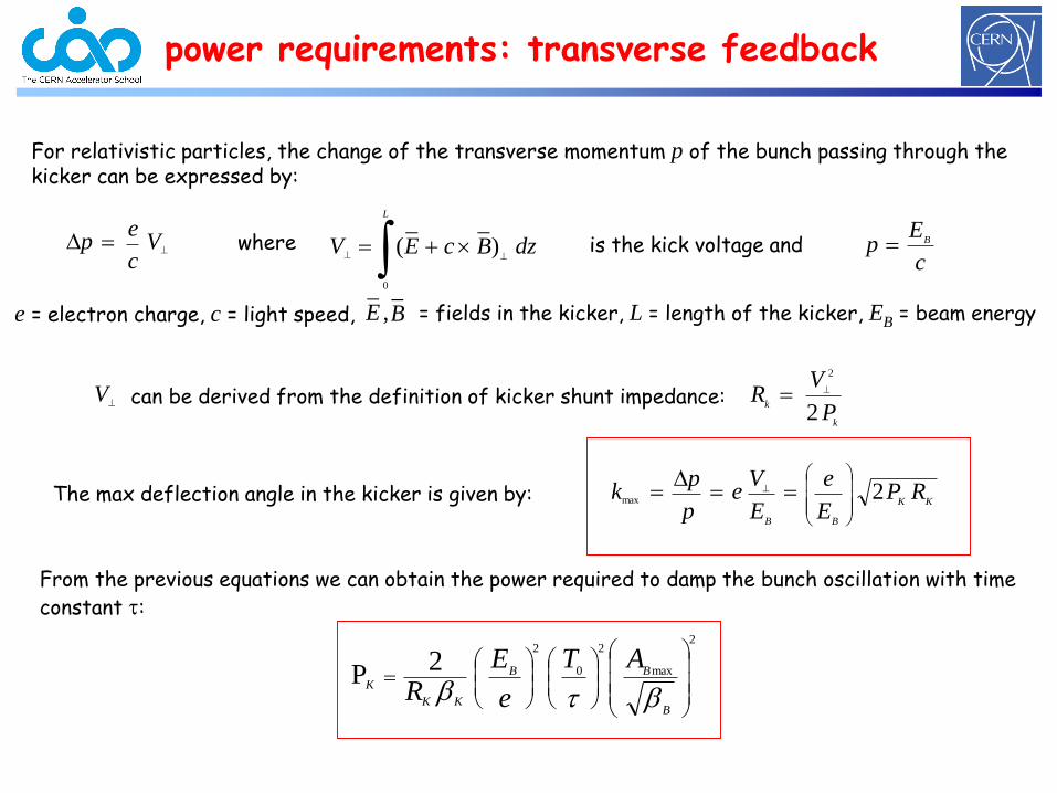
Vc

ep dzBcEV

L

0

)__

(c

Ep B

,_E

_B

For relativistic particles, the change of the transverse momentum p of the bunch passing through the kicker can be expressed by:

where

e = electron charge, c = light speed, = fields in the kicker, L = length of the kicker, EB = beam energy

V can be derived from the definition of kicker shunt impedance:k

k

P

VR

2

2

KK

BB

RPE

e

E

Ve

p

pk 2max

The max deflection angle in the kicker is given by:

From the previous equations we can obtain the power required to damp the bunch oscillation with time

constant :

2

max

2

0

2

2P

B

BB

KK

K

AT

e

E

R

is the kick voltage and

power requirements: transverse feedback