Embed Size (px)
Citation preview

Mule Deer Modeling Report:
A quantitative evaluation of survey efforts to model, monitor and manage
Wyoming mule deer populations
Thomas A. Morrison
Postdoctoral researcher, Wyoming Cooperative Fish and Wildlife Research Unit, Laramie, WY
Matthew J. Kauffman
Unit Leader, Wyoming Cooperative Fish and Wildlife Research Unit, Laramie, WY
APRIL 2014

Deer monitoring final report April 2014
2
Contents
Summary ......................................................................................................................................... 4
Goal: ........................................................................................................................................ 4
Methods: ................................................................................................................................. 4
Introduction and background .......................................................................................................... 7
Study questions ........................................................................................................................... 7
Methods - Simulations .................................................................................................................... 8
Approach ..................................................................................................................................... 8
The Spreadsheet Model............................................................................................................... 8
Simulation ................................................................................................................................... 9
True dynamics ......................................................................................................................... 9
Sampled field data................................................................................................................. 11
Assessing model accuracy .................................................................................................... 11
Assessing ability of model to detect trends........................................................................... 12
Sources of variation in simulations ....................................................................................... 13
Population monitoring scenarios........................................................................................... 13
Monitoring costs summary ....................................................................................................... 14
Herd Composition ................................................................................................................. 14
Harvest survey ...................................................................................................................... 15
Abundance Monitoring ......................................................................................................... 15
Survival monitoring .............................................................................................................. 17
Simulation cost assumptions ................................................................................................. 17
Results ........................................................................................................................................... 17
1. Why are smaller populations more difficult to model? ..................................................... 17
2. How does the addition of abundance estimates affect model performance? ..................... 20
3. If a single field estimate of population abundance is added to a dataset, which year
improves the model the most? .................................................................................................. 22

Deer monitoring final report April 2014
3
4. Can classification be skipped some years and replaces with abundance surveys? Is this
strategy cost effective and what is the best strategy for inputting missing classification data? 23
5. How does the model cope with severe winters (i.e. years where reproduction and survival
are abnormally low)? ................................................................................................................ 24
Conclusions ................................................................................................................................... 25
Relationship between accuracy and cost................................................................................... 25
Future Research Questions ................................................................................................... 27
Acknowledgements ....................................................................................................................... 28
Literature Cited ............................................................................................................................. 28

Deer monitoring final report April 2014
4
Summary Goal: To examine trade-offs between monitoring effort/cost and model accuracy when
estimating post-hunt mule deer herd sizes using the Colorado “Spreadsheet” Model.
Methods: (1) Simulate mule deer population dynamics, (2) sample the simulated populations
under various types and intensities of monitoring data, (3) model the population using the
Spreadsheet Model and the simulated field data, and (4) assess accuracy of the model estimates
of population abundance by comparing them to the simulated “true” population abundances.
Model performance was assessed in two ways: 1) the relative accuracy, measured as the mean
square error, and 2) the probability of correctly detecting a population decline/increase of 5% or
more.
Herd Composition Monitoring
Our analysis relies entirely on the current WGFD monitoring procedures, which rely on the
individual animal as the sampling unit in Classification surveys (i.e. the “Czaplewski”
estimator; Czaplewski et al. 1983). Because the Spreadsheet Model is largely driven by the
herd ratio data, the method for estimating herd composition likely deserves greater
consideration going forward. Because ungulates occur in groups, and individuals within
groups are more likely to be similar to one another in terms of age and sex than those in other
groups, the individual-based method may yield unrealistically precise ratio estimates (i.e. due
to pseudo-replication). Since the Department’s Spreadsheet Models use the standard error
around the classification mean as part of the data fitting process, underestimating this error
(i.e. overly precise estimates) will constrain the model fitting process. “Group-based”
estimators, such as the Bowden estimator (Bowden et al. 2000), resolves several of these
issues by using the group, or how deer are seen on the landscape, and the variation between
groups to more accurately estimate sample error. Since this technique requires the user to
look at more groups in order to get to an acceptable level of sample error, it is likely that
classification survey costs may increase while at the same time resulting in a wider though
more accurate estimated sampling error. Our results suggest that Survival and Abundance
monitoring are not cost effective relative to increasing Classification survey intensity.
However, the relative importance of classification data in the Spreadsheet Model compared
to other data types (survival and abundance estimates) will change (likely becoming less cost
effective) with a change to a different classification estimator.
The “number of animals classified” largely determines the precision of herd ratio estimates,
which in turn largely drives the performance of the Spreadsheet Model under current
monitoring procedures. For key herds and other important herds with a post-season
population objective, annual classification data are critical. However, the cost per animal
classified in Wyoming deer surveys in 2011 varied more than 6-fold (range: $1.41 - $8.67

Deer monitoring final report April 2014
5
per animal). Thus, if there is an immediate need to reduce survey costs, we recommend
focusing survey efforts on priority herds where many animals can be located and classified in
a relatively short period of time.
We recommend against modeling small populations (<1000 individuals in our simulations)
when the intensity of classification surveys is low (fewer than 400 animals), unless there are
other objectives besides that of modeling population trends. Models perform extremely
poorly when classification intensity is low (i.e. 300-400 animals classified or fewer) in all
sized populations, but particularly in small populations (<1000 individuals). If groups are
used as the sampling unit (Bowden estimator), survey intensity will have to be even higher to
provide good model estimates (not part of this analysis).
When composition counts are missed in some years – for example due to priorities elsewhere
or due to budgeting for an abundance survey (see Section 4) – we recommend inserting the
value of the most recent buck:doe ratio and the 4 or 5-yr average fawn:doe ratio in the model.
Using the average values for missing years of buck:doe data results in poor models. This is
because buck:doe ratios are correlated across years, while fawn:doe ratios are mostly
uncorrelated.
Composition counts should never be skipped in years following a severe winter (i.e. the
December following a severe winter). In a severe winter, fawn survival and pregnancy rates
will likely be lower than average. Thus, classification survey results are important the
following year in order to estimate whether survival decreased or not, as inferred from
estimated yearling buck:doe ratios and to detect any decrease in fawn production resulting
from the previous hard winter. Replacing missing herd buck ratios with average values (as
below in Section 4) in the Spreadsheet Model during these years will likely bias the model
estimates high.
Abundance monitoring
Abundance surveys improve model performance under many, though not all, conditions.
One-time, low precision abundance surveys often lower model accuracy, particularly in
medium and large size herds, and are therefore not recommended. Further, abundance
surveys can be costly, and are generally less valuable in terms of gain in model accuracy per
unit cost than an investment in more precise herd ratio data given current monitoring
methodology (see section above).
Abundance surveys provide the greatest value in small populations, in terms of gain in model
accuracy per unit cost. In small populations, even low precision abundance surveys (i.e.,
Coefficient of variation <20%; CV=SD/mean) improve model performance.
In medium and large herds (~9000 and ~25,000 individuals, respectively) abundance surveys
increase model accuracy when they are either (1) conducted very frequently (every 2-3 years)

Deer monitoring final report April 2014
6
and/or (2) conducted at relatively high intensity (Coefficient of variation <15%;
CV=SD/mean). Conducting infrequent AND low-precision abundance surveys (CV=20% or
greater) actually reduces model accuracy on average in medium and large herds because it
adds additional variation to the model. In larger herds where classification and harvest data
are reliable, there appears to be little value in collecting abundance estimates, particularly if
these estimates have low-precision.
Adding two or more abundance surveys, even at low intensity (CV=20%), to a 10-year
dataset generally improves the models, relative to baseline scenarios, in all herd sizes. Thus,
survey intensity should be high (10%) for all initial first-time surveys in the event that they
are not repeated. Subsequent surveys can occur at low (CV=20%) or high intensities (10%)
and still improve the spreadsheet model results. Higher intensity survey will always be more
beneficial.
When using quadrat-based sampling (as in Colorado Parks and Wildlife; see Quadrat
Surveys, page 16), abundance surveys can replace classification surveys in some years while
still improving model performance at comparable cost. For example, consider two
monitoring scenarios: 1) herds are classified every year and 2) herds are classified every two
or three years, but abundance is estimated during the off years at high precision (CV=12%).
Both strategies incur roughly the same cost (assuming abundance can be surveyed similarly
to CPW), but the scenarios with abundance estimates (#2) have higher accuracy. The
exception is when there is a severe winter; then, the scenario with classification surveys
every year (#1) yields better models (see Section 4).
We found no strong rationale for conducting abundance surveys in a given year simply as a
way of “anchoring the models”. Abundance surveys can occur at any time within a series of
data with a similar impact on the model’s performance.
Trend counts cannot be directly incorporated into the Spreadsheet Model; thus we do not
recommend collecting these data for the purpose of generating population estimates.
Survival monitoring
While collecting survival estimates from VHF/GPS collars yielded the most accurate of all
models, survival surveys were also the most expensive survey option to implement, and the
least valuable in terms of gains in model accuracy per unit cost. As an example, monitoring
survival for 10 years using 20 adult collars and 60 juvenile collars yielded only 6-10%
greater model accuracy than monitoring the same herds for abundance every 3 years with
Sightability surveys (assuming a CV of 6%); yet the survival surveys cost roughly 1.5-20
times as much to implement.
If survival surveys are conducted, they are most cost-effective in large populations (>25000
individuals) where other survey options (abundance and classification surveys) are likewise
relatively expensive.

Deer monitoring final report April 2014
7
Introduction and background The Wyoming Game and Fish Department’s survey, data collection, and modeling protocols
have evolved over the years but may not be optimized to allow efficient management of mule
deer and other ungulates under current fiscal, logistical, or environmental constraints. There is a
need to ensure monitoring and modeling practices generate the most accurate and cost-effective
population estimates possible. Model estimates of herd abundance receive considerable scrutiny
from the general public, legislators and other non-management stakeholders due to the economic
and social value of game species. Further, across the western U.S., there is a general call for
standardizing data collection and sharing of ungulate monitoring data to enable needed regional
analyses such as those addressing climate change or habitat alteration (Mason et al. 2006).
In 2012, the WGFD committed to transitioning to the ‘Spreadsheet Model’, developed by
Colorado Parks and Wildlife, for all of its ungulate herd modeling and season setting (White and
Lubow 2002). This model offers a number of practical and statistical advantages over older POP-
series modeling software used by WGFD biologists. Most importantly, the spreadsheet model
incorporates measures of uncertainty (standard error) from monitoring data to produce best-fit
herd size estimates. While the spreadsheet model accommodates multiple sources of monitoring
data, each type of survey data, at each level of intensity, provides a different gain in accuracy for
a given cost to the WGFD. The optimal monitoring approach will likely depend on the species,
the density of herd units, the variability in survival and production of young, and the growth
trajectory of the population.
Given the department’s transition to a new population model at a time of growing fiscal
constraints within the state, there was a need to better understand the efficacy of current and
alternative monitoring and modeling practices. The goal of this study is to examine the many
tradeoffs among potential monitoring and modeling approaches using the Spreadsheet Model.
Our focus is on modeling mule deer populations (i.e. we assume demographic rates are drawn
from a typical mule deer), but many of the results from the study are broadly applicable to most
of Wyoming’s ungulate species.
Study questions
We used simulated data to explore trade-offs in cost, effort, ability to detect herd trends and
model accuracy across a broad range of different monitoring scenarios. The simulations
addressed six main research questions:
1. What are the average costs of monitoring mule deer? Given current monitoring practices,
are there opportunities for cost savings without compromising model performance?
2. How does classification intensity affect model performance?
3. How does the addition of population abundance estimates affect model performance?
4. If a single field estimate of population abundance is added to a dataset, which year
improves the model the most?
Deer monitoring final report April 2014
8
5. Can you improve model accuracy by substituting field estimates of population size for
composition counts? If so, where does this strategy become most cost effective and what
is the best strategy for inputting missing classification data?
6. How does the model cope with severe winters (i.e. years where reproduction and survival
are abnormally low)?
Methods - Simulations
Approach
One of the challenges of modeling field data is that we rarely know the true size of a population,
which means we do not know how well (or poorly) our model has estimated abundance. While
error estimates (e.g. standard error) provide a measure of uncertainty, many population models
suffer from large error, while other models (such as POP-II) simply do not provide a method to
measure error. We addressed this problem by using simulated populations and simulated ‘field
data.’ This approach – increasingly common in the design of monitoring protocols (Nuno et al.,
2013) – allowed us to compare a model estimate of population size (derived from simulated field
data) to a true (simulated) population size. Further, simulations allowed us to explore a large
number of possible monitoring and modeling scenarios (i.e. a large set of parameters). For
example, if we’re interested in understanding whether resources are better used collecting a
single abundance estimate in a 10-year deer dataset versus conducting more precise classification
surveys over that entire period, simulation allows us to control all variables except the ones in
which we are most interested (abundance and precision in age-sex ratios). As in the ‘real world’,
our simulations assumed that populations and field data had some random component, for
example due to winter conditions impacting survival rates. When we simulated a particular
monitoring scenario a large number of times with this random component, the entirety of all
iterations generated a mean set of population estimates and standard errors which could be used
to assess accuracy of the given monitoring scenario. While models are only as good as their
assumptions, the demography of ungulates (mule deer in particular) have been well-studied, so
that we are confident in being able to produce realistic herd dynamics, and realistic field data
based on those herds. We outline this approach in more detail below.
The Spreadsheet Model
The ‘Spreadsheet Model’ is a family of population models that estimates the number of adult
females, adult males and juveniles in a herd across multiple years (White & Ludow 2002). The
number of adults (buck or doe) in a given year (year i) equals the number adults in the previous
year (year i-1) multiplied by their survival rate, plus the number of fawns of that sex that have
survived into adulthood. Finally, the number of animals harvested that year (i) is subtracted from
these totals.
The model incorporates the following types of field data:

Deer monitoring final report April 2014
9
1. Harvest estimates for every year of the model (required)
2. Fawn:Doe ratios for every year of the model (required)
3. Buck:Doe ratios and SE’s for every year of the model (required)
4. Survival rates and SE’s for fawns and/or adults (optional)
5. Abundance and SE’s for a given year (optional)
For more details on the structure of the model, please refer to the WGFD Spreadsheet Model
User Guide.
Simulation
Our simulations consisted of four main steps:
1. Simulate “true” mule deer population abundances
2. Sample the simulated populations under various types and intensities of monitoring data
3. Model the population abundances using the Spreadsheet Model
4. Assess accuracy of the model estimates of population abundance by comparing them to
the simulated “true” population abundances
True dynamics
We simulated the true dynamics of mule deer using an age-structured, post-hunt model that was
split into two age-sex classes: fawns, bucks and does. Survival and fecundity rates were based on
values reported in previous field studies in the Western U.S. (Table 1; Bishop et al. 2005;
Unsworth et al. 2009, Lukacs 2009; Forrester et al. 2012). We assumed vital rates were beta
distributed and constrained between biologically-realistic minimum and maximum values (Table
1).This yielded a mean population growth rate of 0.987.
Age-Class Mean SE Max Min
Fecundity (fawns per doe per year) 1.700 0.120 2.00 0.00
Over-summer fawn survival (0-0.5 years) 0.743 0.052 0.99 0.20
Over-winter fawn survival (0.5-1 years) 0.721 0.094 0.95 0.05
Over-summer yearling survival (1-1.5 years) 0.757 0.018 0.99 0.40
Over-winter yearling survival 0.935 0.007 0.99 0.70
Annual adult survival (1.5+ years) 0.840 0.048 0.99 0.65
Table 1. Mule deer demographic rates used to project ‘true’ population dynamics in this study.
We assumed adults are harvested each year based on the distribution of harvest rates reported in
the North Bighorn mule deer herd from 1982-2007 (26 years). We chose the North Bighorn herd
to reflect harvest intensity in our simulation because this herd appeared to have continuous and
relatively stable harvest rates over a long period of time. Further, the herd was relatively isolated
so does not have major interchange issues, compared to some herds. Harvest rates from this herd

Deer monitoring final report April 2014
10
were calculated as the proportion of the pre-hunt population in each age-sex class harvested in a
given year, based on harvest survey estimates and POP-II population values reported in WGFD
Annual Big Game Reports (Table 2). After confirming normality of North Bighorn harvest rates,
we randomly sampled from the distribution of harvest rates. Actual harvest numbers in a given
year were scaled to the previous year’s population size, so that larger populations had larger
harvests. Overall, total harvests averaged 10.1% of the pre-hunt population size.
Table 2. North Bighorn mule deer survey and POP-II model results 1982-2007, Wyoming Game and Fish
Department.
For each monitoring scenario, we simulated the same 25 independent populations by randomly
selecting different combinations of survival and harvest. Each of these populations was sampled
200 times to generate representative field data. Finally, population abundance was estimated
using the Spreadsheet Model (for a total of 5000 simulations per monitoring scenario). This
approach allowed us to estimate a sampling variance for each population trajectory (see
following section). Each projected population started at one of three initial sizes (small: 2000
individuals; medium: 20,000 individuals; large: 50,000 individuals) and was projected for 50
Buck Doe Fawn Total
1982 1860 319 0 2179 12629 NA NA
1983 1287 410 44 1741 14304 NA NA
1984 1128 372 33 1533 11700 2.3 73.5
1985 1160 601 41 1802 11745 3.4 66.6
1986 1302 555 43 1900 11267 8.9 61.7
1987 1382 510 45 1937 14800 10.4 76.1
1988 1613 370 27 2010 12483 11.9 76.9
1989 1429 517 35 1981 12918 11.8 71.3
1990 1222 752 53 2027 13184 11.7 69.4
1991 1640 724 28 2392 23071 13.5 76.5
1992 1590 1160 54 2804 22687 15.0 67.6
1993 1610 1124 51 2785 17831 14.5 66.9
1994 1272 853 38 2163 17796 14.7 61.9
1995 1062 580 40 1682 18561 15.3 62.4
1996 1796 556 21 2373 19941 12.3 65.3
1997 1107 172 10 1289 15994 12.5 66.0
1998 1549 106 13 1668 18297 13.6 67.9
1999 1735 114 7 1856 22826 11.4 71.7
2000 1738 168 12 1918 20328 10.7 58.3
2001 1315 272 22 1609 20060 15.2 63.0
2002 1187 227 40 1454 20435 12.6 66.3
2003 1359 154 22 1535 21533 13.5 73.9
2004 1601 285 16 1902 23959 10.6 76.8
2005 1652 401 32 2085 23247 15.5 71.7
2006 1713 456 33 2202 25410 18.3 76.9
2007 1389 661 27 2077 26404 23.0 68.3
Buck:Doe Fawn:DoeHarvest
Year POP-II Est.

Deer monitoring final report April 2014
11
years into the future. We used only the final 10 years of these projections to minimize potential
effects of initial conditions.
Sampled field data
Simulated field data were sampled from the 10-year ‘true’ population projections. We treated
herd classification samples as random normal variables, with mean equal to the true age-sex
ratio; thus, we assumed there was no bias in classification. Sample estimators were based on the
Czaplewski et al. (1983) approach. We examined a range of classification intensities (i.e. the
proportion of the population that was classified): 12%, 15%, 18% or 30%. For comparison, in
Wyoming in 2011 the average proportion of mule deer herds classified was roughly 25%.
We collected harvest samples from the true harvest rates (mentioned above), assuming that the
samples came from a random normal distribution. Harvest rates were inclusive of wounding loss.
We also assumed that 95% of harvest samples were within 10% of the true harvest, similar to the
error rate reported from the Wyoming deer harvest survey for many herds.
Field estimates of survival were sampled from the true survival rates assuming random binomial
sampling, where the number of samples equaled the number of VHF radio collars (either 20 or
40 for adults, and 60 or 120 for fawns). SE of these samples was calculated from the sample size
and survival rate.
Abundance estimates were likewise sampled from the true population abundance assuming
samples derived from a random normal distribution. We sampled abundance at a high, medium
and low precision, equivalent to Coefficients of Variation = 6%, 12% and 20%, respectively. We
also assumed equal sightability of all age-sex classes.
Assessing model accuracy
We used a similar model as the Spreadsheet Model but built in the program R (R: Development
Core Team 2009), developed by Paul Lukacs (University of Montana). Using R allowed us to
simulate population data and run models over a large numbers of conditions and parameters,
which would have been unmanageable in Microsoft Excel. The only difference in models
between the Excel and R versions is that the R version uses a more powerful optimization
procedure called maximum likelihood (‘optim’ function in R) in place of Excel’s Solver.
Maximum likelihood is a standard statistical approach used to find optimal parameter values.
Importantly, we chose to use only one survival model – #2 in the spreadsheet model (constant
adult survival, time-varying fawn survival) rather than compare multiple models using AICc, to
reduce the sizable computational demands of the simulation. Following White and Lubow
(2002), we assumed the fawn sex ratio was 0.5 and that buck and doe survival rates were equal.
We also used a starting population of twelve times the mean buck harvest for the first 5 years,
which serves as a rough rule of thumb when approximating population size. The starting adult

Deer monitoring final report April 2014
12
and fawn survival values were 0.87 and 0.57, respectively, which is the mean annual survival for
these age classes.
We used several common metrics for comparing the performance of different field monitoring
scenarios: bias, precision (SE) and accuracy (root mean squared error).
n
NN
NBias
n
i
i
1
)ˆ(
)ˆ(
1
)ˆˆ(
)ˆ( 1
2
n
NN
NSE
n
i
i
1
)ˆ(
)ˆ(
2
1
n
NN
NRMSE
n
i
i
Because we modeled 25 population trajectories 200 times each for every scenario, we report the
overall mean of the bias, Standard Error (SE) and Root mean square error (RMSE) for each
scenario across all simulations. Ultimately model performance is based on RMSE, which is a
measure of total model accuracy, a combination of bias and SE. Higher RMSE implies a less
accurate model. Thus, most of the focus of the results is on this error metric.
Assessing ability of model to detect trends
Additionally, we measured the probability that the model correctly detected changes in the
population size. We did this by measuring the proportion of years where the true population size
increased or decreased by more than 5% while the model estimates indicated a population
change in the opposite direction (by any amount). For example, if the true population declined by
8% between two years, we judged the model estimates as having detected the decline incorrectly
if the model indicated that the population increased.
Similarly, we were interested in the probability that the model produced a trend (increasing or
decreasing) when there was no trend present (i.e. false positives). We measured the proportion of
years where the model indicated a >5% population change, while the true population trends were
changing in the opposite direction. For instance, if our model suggested a 11% increasing
population trend, but the true trend was a -1% decrease (or vice versa), we deemed this a false
positive.

Deer monitoring final report April 2014
13
Sources of variation in simulations
Our simulations produced two types of variance: process variance and sampling variance (Figure
1). Process variance is caused by random variation in survival and fecundity rates from year to
year within the true population. Sampling variance, in contrast, was generated from sampling the
true population and modeling a given set of sample data. In the analysis, we are mostly interested
in sampling variance. However, model results will vary depending on the specific trajectory of
the true population, so it is important to allow for some process variance in the simulation.
Figure 1. Illustration of the sources of variation in the simulations (n=500 iterations).Process variance (A)
shows the variance of true population sizes and 95% confidence intervals (dotted red lines) around the mean
population trend (black line). Each grey line in (A) is a single iteration with randomly drawn vital rates and
harvest rates. Sampling variance (B) is the variance due to the sampling of herd composition data surrounding a
single population trend (black line). Each grey line in (B) is a single iteration of model-derived population
estimates in which the true population had invariable vital rates and harvest rates each year (i.e. we held the true
population constant). Only field herd composition data are used in the model. Note that model-derived
population estimates (B) are more precise during the middle of the data series than at the beginning or end.
Population monitoring scenarios
Following discussions with WGFD biologists, we identified a set of core monitoring scenarios
which differ only slightly from current monitoring approaches in terms of cost and effort, and
would therefore be the most feasible scenarios to implement. These core monitoring scenarios
are concerned with either (1) herd classification survey intensity, (2) trade-off between
A B

Deer monitoring final report April 2014
14
substituting abundance estimates for classification estimates in some years, (3) optimal timing
for a “one off” field estimate of herd abundance to improve model accuracy, or (4) the impact of
a severe winter on model results. Note that many of the results of these core monitoring
scenarios are presented as being relative to “baseline”. The baseline is the one most similar to
current monitoring practices in Wyoming, which includes medium-intensity classification (18%
of the herd is classified) and annual harvest surveys.
Because we were interested in exploring the capabilities of the spreadsheet model under a large
number of circumstances, we also examined several additional scenarios that would require
substantial increases in cost and effort, such as those involving survival monitoring and annual
abundance estimation. We evaluated model accuracy across three population sizes: small (1000
individuals), medium (9000 individuals) and large (25000 individuals). For the medium
population size, we evaluated the impact of a severe winter (occurring in year 5 of the dataset),
in which fawn survival and adult fecundity were reduced by 60% and adult survival was reduced
by 30%. This large set of survey scenarios allowed us to ask a set of specific questions related to
power and cost.
Monitoring costs summary
The cost of a particular monitoring strategy for any ungulate population depends on a large
number of factors, including survey intensity, survey type, survey area, herd density, weather
conditions, transport distance of survey vehicles, sightability, collar type (for survival
monitoring), etc. Thus, cost will vary greatly from one situation to another. Our goal here was to
summarize the average survey costs for a herd of average density to provide insight into the
relationship between model precision and cost, or literally “bang for your buck”.
Herd Composition
For classification surveys, we solicited information from WGFD biologists across the state about
survey costs in 2011, number of animals classified and hours spent classifying (Table 3). Since
the precision of herd ratio estimates largely depends on the number of animals classified
(Czaplewski et al. 1983), we calculated a cost per animal classified. For mule deer, the cost per
animal classified ranged widely, from $1.41 to $8.67 per animal. The greater cost in some areas
appeared to be at least partly due to lower herd densities and more challenging cover and terrain
within these sampling areas. The “number of animals classified” largely determines the precision
of herd ratio estimates, which in turn largely drives the performance of the spreadsheet model.
Thus, if there is an immediate need to reduce survey costs, there may be opportunities to target
specific areas or herd units where many animals can be classified in a relatively short period of
time.

Deer monitoring final report April 2014
15
Table 3. Classification costs of high-priority herds in Wyoming, from WGFD big game biologists in 2011.
Elk are included here for comparison.
Harvest survey
For harvest survey costs, we converted the harvest survey budget for deer ($342,000 = total
harvest survey budget in FY12, of which 44% went towards deer classification) into a survey
cost per animal harvested ($2.98/harvested deer) (Table 4). Harvest surveys are largely mail-
based surveys and most surveys are contracted to a private company that specializes in compiling
harvest surveys.
Table 4. Approximate harvest survey cost summary, WGFD 2010.
Abundance Monitoring
Our simulations sampled abundance at a low, medium and high intensity, equivalent to
Coefficients of Variation = 20%, 12%, and 6%, respectively. At CV=6%, the population estimate
is within 10% of the true herd size 90% of the time. Costs for these sampling intensities were
based on Sightability surveys.
Sightability Survey.
WGFD recently implemented Sightability surveys for estimating abundance. This technique,
originally developed in Idaho, involves counts from helicopters that correct for variation in
detectability across different habitat types, group sizes and snow cover (among other variables)
Spp. Herd UnitPost-hunt Pop Est
(2009)
Total animals
classified
Hours
flownTotal cost
Class-
cost/hour
Class-
cost/animal
DEER Baggs Mule 16300 4291 12 $9,500 $792 $2.21
DEER Bates Hole/Hat Six 8000 1300 12.5 $11,000 $880 $8.46
DEER Powder River 52400 2590 6 $5,700 $950 $2.20
DEER South Wind River 11600 3000 33 $26,000 $788 $8.67
DEER Sublette 29000 8800 18 $12,420 $690 $1.41
DEER Wyoming Range 29000 7700 20 $13,800 $690 $1.79
ELK Laramie Peak/Muddy Mountain 9815 4650 18 $16,000 $889 $3.44
ELK Piney 3511 2563 3 $2,070 $690 $0.81
ELK Sierra Madre 8957 4960 15 $12,000 $800 $2.42
ELK South Wind River 4000 3000 13 $10,000 $769 $3.33
ELK West Green River 3878 3200 18 $15,000 $833 $4.69
ELK Wiggins Fork 7034 3110 12 $10,000 $833 $3.22
Species#Animals Harvested
(2010)
Harvest Survey
Costs (approx)
Harvest survey cost per
animal harvested
Elk 25,672 $116,354 $4.53
Mule Deer 34,469 $102,665 $2.98
Pronghorn 58,863 $75,288 $1.28
White-Tailed Deer 14,650 $47,911 $3.27
TOTAL 133654 $342,218
Deer monitoring final report April 2014
16
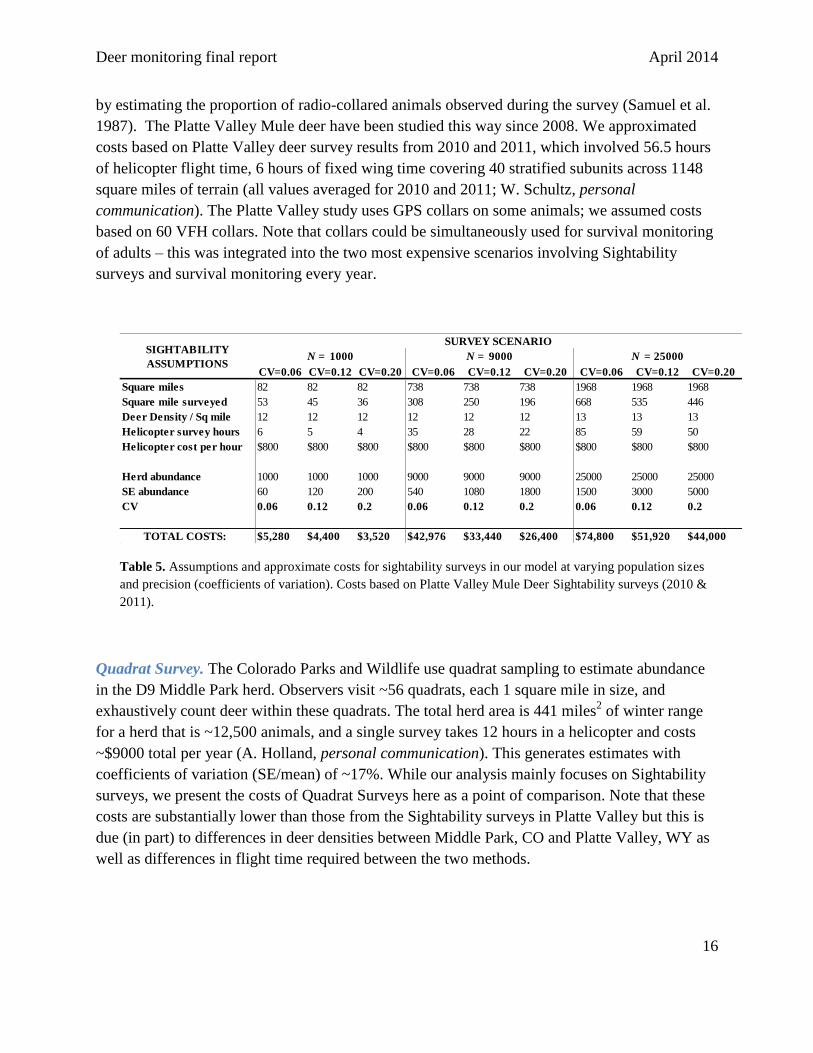
by estimating the proportion of radio-collared animals observed during the survey (Samuel et al.
1987). The Platte Valley Mule deer have been studied this way since 2008. We approximated
costs based on Platte Valley deer survey results from 2010 and 2011, which involved 56.5 hours
of helicopter flight time, 6 hours of fixed wing time covering 40 stratified subunits across 1148
square miles of terrain (all values averaged for 2010 and 2011; W. Schultz, personal
communication). The Platte Valley study uses GPS collars on some animals; we assumed costs
based on 60 VFH collars. Note that collars could be simultaneously used for survival monitoring
of adults – this was integrated into the two most expensive scenarios involving Sightability
surveys and survival monitoring every year.
Table 5. Assumptions and approximate costs for sightability surveys in our model at varying population sizes
and precision (coefficients of variation). Costs based on Platte Valley Mule Deer Sightability surveys (2010 &
2011).
Quadrat Survey. The Colorado Parks and Wildlife use quadrat sampling to estimate abundance
in the D9 Middle Park herd. Observers visit ~56 quadrats, each 1 square mile in size, and
exhaustively count deer within these quadrats. The total herd area is 441 miles2 of winter range
for a herd that is ~12,500 animals, and a single survey takes 12 hours in a helicopter and costs
~$9000 total per year (A. Holland, personal communication). This generates estimates with
coefficients of variation (SE/mean) of ~17%. While our analysis mainly focuses on Sightability
surveys, we present the costs of Quadrat Surveys here as a point of comparison. Note that these
costs are substantially lower than those from the Sightability surveys in Platte Valley but this is
due (in part) to differences in deer densities between Middle Park, CO and Platte Valley, WY as
well as differences in flight time required between the two methods.
N = 1000 N = 9000 N = 25000
CV=0.06 CV=0.12 CV=0.20 CV=0.06 CV=0.12 CV=0.20 CV=0.06 CV=0.12 CV=0.20
Square miles 82 82 82 738 738 738 1968 1968 1968
Square mile surveyed 53 45 36 308 250 196 668 535 446
Deer Density / Sq mile 12 12 12 12 12 12 13 13 13
Helicopter survey hours 6 5 4 35 28 22 85 59 50
Helicopter cost per hour $800 $800 $800 $800 $800 $800 $800 $800 $800
Herd abundance 1000 1000 1000 9000 9000 9000 25000 25000 25000
SE abundance 60 120 200 540 1080 1800 1500 3000 5000
CV 0.06 0.12 0.2 0.06 0.12 0.2 0.06 0.12 0.2
TOTAL COSTS: $5,280 $4,400 $3,520 $42,976 $33,440 $26,400 $74,800 $51,920 $44,000
SIGHTABILITY
ASSUMPTIONS
SURVEY SCENARIO

Deer monitoring final report April 2014
17
Survival monitoring
For survival monitoring we assumed each VHF collar cost $700 for materials, deployment and
monitoring ($400/collar + $200 for capture + $100 for monitoring/collar/year). Fawn survival
monitoring was more expensive than adult survival monitoring because it required redeploying
collars each year on a new cohorts of animals. Adult survival monitoring only required
replacement of collars after the animal or the battery died (assumed survival at the mean annual
adult rate: 0.87; battery needs replacing every four years).
Simulation cost assumptions
In our simulations, we assumed the cost of classification flights was linearly related to the total
number of animals classified. The simulated herds were classified across a range of sampling
intensities, and we converted these into a cost estimate assuming a mean herd size and mean
coverage area from Table 6.
Table 6. Cost assumptions per year used in this study. See text for description of herd density, herd size and material
costs of each monitoring scenario.
Results
1. Why are smaller populations more difficult to model?
Small populations are the most challenging to model in the Spreadsheet Model because they are
the most sensitive to variation in quality of field data. If harvest and classification surveys are
imprecise in some years (which is likely in small populations), fitting reasonable survival rates
Pop size = 1000 Pop size = 9000 Pop size = 25000
Harvest Survey $349 $3,145 $8,737
Classification - vLow intensity (12% herd classified) $360 $3,235 $8,986
Classification - Low intensity (15% herd classified) $450 $4,044 $11,233
Classification - Medium intensity (18% herd classified) $539 $4,843 $13,480
Classification - High intensity (30% herd classified) $898 $8,088 $22,465
Sightability-Low precision (CV=20%) $3,520 $26,400 $44,000
Sightability-Med precision (CV=12%) $4,400 $33,440 $51,920
Sightability-High precision (CV=6%) $5,280 $42,976 $74,800
Survival juvenile - 60 collars $42,000 $42,000 $42,000
Survival juvenile - 120 collars $84,000 $84,000 $84,000
Survival adult - 20 collars $6,993 $6,993 $6,993
Survival adults - 40 collars $13,986 $13,986 $13,986
Survival juvenile 60 collars + Survival adult 20 collars $48,993 $48,993 $48,993
Survival juvenile - 120 collars $84,000 $84,000 $84,000
Survival juvenile 120 collars + Survival adults 40 collars $97,986 $97,986 $97,986
Cost per YearSurvey Data Type

Deer monitoring final report April 2014
18
becomes extremely difficult. Often the result is that the population crashes or explodes, though
adding constraints to the survival rates reduces this effect. In our simulations, herds of 1000
individuals modeled poorly when fewer than 40% of the herd were classified (Figures 2 & 3). In
small populations, model estimates were 107 times more accurate (yes, you read that right) when
40% of the herd was classified compared to 10%. Yet, the cost per year of increasing sampling
intensity from 10% of the herd to 40% of the herd in small herds was just over $800, or one
additional hour of helicopter flying time. In medium size herds (9000 individuals) there was only
a 7-fold difference in accuracy between classifying 10% and 40% of the herd. We did not
examine large herds in this set of simulations because of computing limitations.
Figure 2. Relationship between classification intensity and relative model accuracy (lower Rel MSE is
better) and correct trend detection across two herd sizes, small (red) and medium (blue). Model accuracy in
the small herd (red) was extremely poor when classification intensity was below 40%. In these sets of
monitoring scenarios, no large-sized herds were examined.
Deer monitoring final report April 2014
19
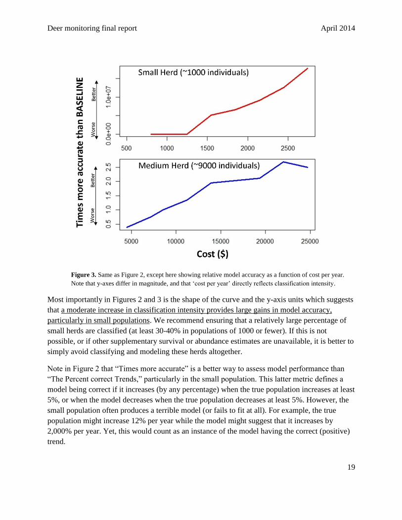
Figure 3. Same as Figure 2, except here showing relative model accuracy as a function of cost per year.
Note that y-axes differ in magnitude, and that ‘cost per year’ directly reflects classification intensity.
Most importantly in Figures 2 and 3 is the shape of the curve and the y-axis units which suggests
that a moderate increase in classification intensity provides large gains in model accuracy,
particularly in small populations. We recommend ensuring that a relatively large percentage of
small herds are classified (at least 30-40% in populations of 1000 or fewer). If this is not
possible, or if other supplementary survival or abundance estimates are unavailable, it is better to
simply avoid classifying and modeling these herds altogether.
Note in Figure 2 that “Times more accurate” is a better way to assess model performance than
“The Percent correct Trends,” particularly in the small population. This latter metric defines a
model being correct if it increases (by any percentage) when the true population increases at least
5%, or when the model decreases when the true population decreases at least 5%. However, the
small population often produces a terrible model (or fails to fit at all). For example, the true
population might increase 12% per year while the model might suggest that it increases by
2,000% per year. Yet, this would count as an instance of the model having the correct (positive)
trend.

Deer monitoring final report April 2014
20
2. How does the addition of abundance estimates affect model performance?
Model accuracy generally improves when field estimates of herd abundance can be conducted
and added to datasets (Figure 4). Abundance estimates provide the largest relative benefits –
given their cost – in small populations. However, if abundance estimates are imprecise, they can
actually reduce model accuracy (see points below the dotted line in Figure 4). This occurs when
other field data (namely classification data) are precise, but abundance estimates introduce
additional noise (i.e. uncertainty) to the model estimates.
Figure 4. Relationship between relative survey cost (x-axis) and relative model accuracy (y-axis) across
three herd sizes: ~1000 animals, ~9000 animals and ~25,000 animals herd size and three Sightability
survey intensities (CV = 6%, 12% and 20%). All scenarios involve only a single abundance estimate within
a 10-year data series, and all values are relative to a “baseline” monitoring scenario, where monitoring data
include medium-intensity classification (18% of herd is classified) only. Note that the x-axis is on a relative
scale, so increasing cost from 1 to 1.5 in the largest herd is more expensive in absolute terms than
increasing the same percentage in the medium or small-sized herds. Also note that the y-axis differs
between the small population and the medium and large populations. Thus, in the small population a single
abundance estimate with CV=20% improves the model 580 times relative to baseline.
In small herds (~1000 animals), abundance surveys are inexpensive in absolute terms, though not
in relative terms. However these surveys – even at low intensity (CV=20%) – will strongly

Deer monitoring final report April 2014
21
benefit model results compared to the baseline situation. In contrast, abundance surveys of large-
sized herds (~25,000 animals) can actually generate lower accuracy than baseline if survey
intensity is low (CV > 12%). Note these results (Figure 4) apply specifically to 10-year datasets
containing a single abundance estimate.
Figure 5. Abundance survey intensity vs. model accuracy, relative to baseline, across a range of herd sizes
and survey frequencies (red numbers: 1, 2, 3 or 5 surveys per 10-years). Values above 1.0 on the y-axis
indicate monitoring scenarios that produce better model estimates than those of baseline (i.e. better than a
scenario with only classification surveys at medium intensity, 18% of herd of a given size is classified).
When abundance surveys are conducted multiple times over a 10-year span (Figure 5), model
accuracy improves but may still not be worth the cost, particularly in large-sized herds
(N=25,000). Large herds have more precise classification and harvest data than medium and
small-sized herds, so the models for large herds are less sensitive to ancillary data such as
abundance estimates. Figure 5 shows that, in a large herd, even when abundance is collected 5
times over a 10-year dataset (i.e. every other year), model accuracy only improves (at most) by
2-fold. This 2-fold increase in accuracy would require high-precision surveys (CV=6%) costing
$74,800 per year. Thus, in larger herds where classification and harvest data are reliable,
there appears to be little value in collecting abundance estimates, particularly if these
estimates have low-precision.
Overall, low-precision abundance surveys (CV=20%) always led to poorer models (relative to
baseline) in all medium- and large-sized herds (Figure 5). This suggests that conducting an

Deer monitoring final report April 2014
22
abundance survey does not necessarily yield better models; survey precision must remain
relatively high. Models with high precision abundance surveys always produced better models
regardless of herd size.
3. If a single field estimate of population abundance is added to a dataset,
which year improves the model the most?
As the WGFD transitions to the Spreadsheet Model, one monitoring option is to conduct
abundance surveys during the early years of the transition as a way of ensuring the starting
population sizes (a key assumption in the Spreadsheet Model) are close to reality. Thus, we
wanted to know whether abundance estimates at the beginning of a data series would “anchor”
the model more effectively than waiting to conduct a survey in later years.
Our results suggest that field estimates of population abundance had the largest impact on model
performance if added to the middle years of a dataset, rather than in the first or last year (Figure
6). The greatest accuracy and detection of trends was achieved by adding an abundance estimate
to year 7. However, accuracy and trend detection did not vary substantially in our simulation: the
difference between the lowest and highest values was only 16% for accuracy and 2% for trend
detection, suggesting that the year in which population abundance is added does not have a large
impact on model performance. Thus, the year in which surveys are conducted does not
substantially impact model accuracy. Obviously, managers do not have the luxury of selecting
the particular year in which a survey falls within a given dataset. However our results suggest
that surveys need not be conducted from the onset of using the Spreadsheet Model for good
model performance.
Figure 6. Relationship between the timing (year) of the abundance estimate within a data series and model accuracy.
Note the relatively small degree of variation in either y-axis.

Deer monitoring final report April 2014
23
4. Can classification be skipped some years and replaces with abundance
surveys? Is this strategy cost effective and what is the best strategy for
inputting missing classification data?
The Spreadsheet Model requires classification survey data be inputted every year. However,
because of field constraints or because of alternative monitoring strategies, classification sruveys
may be missed in certain years. Here we examine an alternative monitoring in which
classification surveys are skipped some years, but abundance surveys are conducted instead.
Skipping classification surveys and substituting some missing years with abundance surveys
generally improves model accuracy relative to baseline, particularly in small populations (Figure
7). However, because of the high cost of Sightability surveys, replacing classification surveys
with occasional abundance surveys always incurs a higher cost relative to baseline. In our
analysis, we assumed that classification and abundance surveys were each conducted either
every 2 years or every 4 years (Figure 7).
Our results suggest that in small populations, skipping classification surveys and conducting
occasional abundance surveys also generates much better model estimates than baseline at a
relatively low additional cost. Thus, this strategy is most cost-effective in small, high priority
populations, particularly if the cost of abundance surveys is not much greater than classification
surveys. In larger populations, skipping classification surveys and replacing them with
abundance surveys is only worthwhile (though still costly) if survey intensity is relatively high
(CV=12% or 6%). Note that these results are contingent on the assumption that abundance
survey costs are based on Sightability surveys. Costs associated with quadrat sampling from
CPW suggest that this strategy (i.e. skipping classification and conducting occasional abundance
surveys) every 4 years is actually cheaper than baseline. More information about the quadrat
sampling method is needed to explore its applicability to Wyoming herds.
There are various ways to input the missing classification data in the Spreadsheet model. In
Figure 7, the best strategy for inputting missing Fawn:Doe data is to take the 4-year average of
Fawn:Doe ratios and SE estimates. A separate analysis (figure not included) suggests that the
best overall strategy for missing Buck:Doe data is to simply use the most recent buck:doe count
and SE. This is because Buck:Doe ratios are correlated across years, while Fawn:Doe ratios are
largely uncorrelated.

Deer monitoring final report April 2014
24
Figure 7. Monitoring scenarios in which abundance and classification surveys each occur every 2 or 4
years. Three strategies for modeling the missing Fawn:Doe data in the Spreadsheet Model: (1) take the 4
year recent average (blue line), take the 10-year average (red line) or take the most recent value (green
line). All values are relative to baseline, i.e. the monitoring scenario in which only medium intensity
classification survey data are modeled. X-values greater than 1.0 are more expensive than baseline, while
Y-values above 1.0 are more accurate than baseline.
5. How does the model cope with severe winters (i.e. years where
reproduction and survival are abnormally low)?
Severe winters increased the importance of including composition counts in the model each year.
Models that used mean composition data in some years did a poor job of identifying the correct
trends. For example, when classification data were NOT collected each year, the models only
identified the correct population trend 47-62% of runs. This occurred even if the monitoring
datasets included field estimates of herd abundance. When herd composition data were collected
every year (even with low precision and no supplementary field data), the models identified the
correct trend 76%-96% of the time (Figure 8).

Deer monitoring final report April 2014
25
Figure 8. Effect of a severe winter on model performance. Each point represents a different monitoring
scenario, with 5000 iterations. Only years where the true population changed by at least 5% were included.
Models that lacked herd composition data every year (scenarios below the grey dotted line) performed
poorly, even when field estimates of abundance were included in the model.
Conclusions
Relationship between accuracy and cost
Our main interest was to identify monitoring scenarios that provide the most cost-effective and
accurate population estimates, using the Spreadsheet Model. We found that as monitoring
costs/effort go up, there are diminishing returns in terms of model accuracy (Figures 8-9). Many
of the more expensive scenarios would be impractical to implement in Wyoming. However,
importantly, current monitoring practices in Wyoming are near the inflection point of the cost-
benefit curve. This indicates that small changes to monitoring practices – either slightly more or
slightly less cost/effort – can have large impacts on model accuracy. For example, Figure 9
below shows the relationship between accuracy (low values are more accurate) and relative cost
in the medium size population (9000 individuals). The blue arrow indicates one scenario that
improves accuracy by almost 2-fold, at a marginally higher cost than baseline (red dot). This
particular scenario involves simply collecting high-precision classification data during
composition surveys (i.e. classifying 30% of the herd rather than 18% in the baseline), which in
our simulations translates into an additional $2500 in survey costs per year, or 40% more than
the baseline.

Deer monitoring final report April 2014
26
Figure 9. Relationship between relative survey cost/effort and model accuracy across 38 possible
monitoring scenarios for a medium sized herd (N=9000 individuals). The red dot indicates the baseline
scenario in which 18% of the herd is classified and the blue arrow indicates a cost-effective scenario where
30% of the herd is classified.
Our results suggest that the biggest bang for your buck (or, improvement in model accuracy per
unit cost) comes by increasing classification survey intensity. Abundance and Survival surveys
generally improve model performance, but they do it at a high relative cost. Importantly, this
result is contingent on the methodology used for classification counts – as mentioned earlier, the
Czaplewski estimator provides extremely high estimates of precision (perhaps misleadingly
high), which strongly drive the model’s performance. If WGFD were to use a ’group-based’
estimator (e.g. Bowden et al. 2000), abundance and survival surveys would almost certainly
become more cost-effective and valuable. This likely explains at least some of the discrepancy
between our results and those from scientists in Colorado, who advocate survival monitoring
(White & Lubow 2002). Group-based estimators such as the Bowden estimator generate
considerably larger SE estimates than those currently used by WGFD. The problem with the
individual-based classification estimators is two-fold: (1) classification data may be biased, for
example due to sightability differences between age-sex classes, or between does with fawns
versus though without fawns and (2) the composition of groups of animals tend to be correlated,
so that counting individuals within groups is akin to pseudo-replication. Because the
Spreadsheet Model weighs the field composition data by its SE, having misleadingly accurate or

Deer monitoring final report April 2014
27
precise ratio estimates will have a considerable impact on model results, particularly when no
other supplementary data (abundance or survival estimates) are used in the model.
Furthermore, there are additional reasons (not considered in the present analysis) to conduct
Survival or Abundance monitoring than simply to include a single estimate in a single population
model. For instance, current work by Paul Lukacs (University of Montana) suggests that survival
rates are correlated between adjacent herds and that this correlation can be estimated, suggesting
that survival rates for one herd can be used to infer survival rates in adjacent herds. Further,
collars are obviously an important tool for monitoring movement patterns and interchange
between herds. Abundance monitoring provides useful information on the distribution of animals
on the landscape.
Our analysis is specifically concerned with the relationship between model accuracy and direct
monitoring costs. Obviously there are numerous benefits to monitoring that are not directly
reflected here. For instance, our analyses suggest that monitoring survival rates with collars
yields only marginal gains in precision for a considerable cost investment. However, collaring
data yield important insight into the degree of herd closure, which is a major assumption in
ungulate modeling. Knowledge of interchange may improve modeling efforts. The violation of
the closure assumption can strongly impact and bias model estimates. Further, collaring provides
a means for estimating sightability coefficients, which are critical for obtaining unbiased
abundance estimates.
While biologists must weigh a large number of factors when determining how best to survey
mule deer given finite resources, our simulation approach provides insight into this highly
dimensional problem. This approach and supplementary R-code could be modified to examine a
host of other possible scenarios, involving different herd sizes, population trends, mean vital
rates, species, etc.
Future Research Questions
1. How does classification methodology (i.e. individual-based vs. group-based estimators)
influence model performance?
2. What are the trade-offs between Quadrat-based and Sightability surveys?
3. What is the impact of the dataset length? I.e., do long (20 years) datasets perform better
than short (10 years) or very short (5 years) datasets?
4. Should new models (and data series) be started following severe winters?
5. How does the harvest survey impact model accuracy? Since the model assumes harvest
estimates do not contain any error, how much of an effect does greater/lower precision of
harvest estimates have on model accuracy?
6. How does violation of the herd closure assumption influence model estimates?

Deer monitoring final report April 2014
28
Acknowledgements
The study would not have been possible without substantial input and support from Bob Lanka,
Jeff Short, Greg Anderson and Daryl Lutz, as well as numerous other big game biologists in the
Wyoming Game and Fish Department. Bob in particular provided valuable feedback on
numerous drafts of this report. Will Schultz was extremely helpful in collating information about
Sightability surveys. We also thank biologists in the Colorado Parks and Wildlife, in particular
Andy Holland and Paul Lukacs (now at the University of Montana), who provided considerable
input. Andy patiently responded to numerous inquiries about the Spreadsheet Model and CPW
survey methods. Paul was instrumental in his technical advice and helped develop the
Spreadsheet Model in R, which was used to run the simulations.
Literature Cited
Bishop, C.J., White, G.C., Freddy, D.J. & Watkins, B.E. (2005). Effect of limited antlered
harvest on mule deer sex and age ratios. Wildlife Society Bulletin, 33: 662-668.
Bowden, D.C., White, G.C., Bartmann, R.M., 2000. Optimal allocation of sampling effort for
monitoring a harvested mule deer population. Journal of Wildlife Management, 64, 1013-1024.
Czaplewski, R.L., Crowe, D.M. & Mcdonald, L.L. (1983). Sample sizes and confidence intervals
for wildlife population ratios. Wildlife Society Bulletin, 11: 123-128.
Forrester, T.D., Wittmer, H.U., 2012. A review of the population dynamics of mule deer and
black-tailed deer Odocoileus hemionus in North America. Mammal Review, 43, 292-308.
Lukacs, P.M., White, G.C., Watkins, B.E., Kahn, R.H., Banulis, B.A., Finley, D.J., Holland,
A.A., Martens, J.A. & Vayhinger, J. (2009). Separating Components of Variation in Survival of
Mule Deer in Colorado. Journal of Wildlife Management, 73: 817-826.
Nuno, A., Bunnefeld, N. & Milner-Gulland, E.J. (2013) Matching observations and reality: using
simulation models to improve monitoring under uncertainty in the Serengeti. Journal Applied
Ecology, 50, 488-498.
R: Development C. Team (2009) R: A Language and Environment for Statistical Computing. R
Foundation for Statistical Computing, Vienna.
Samuel, M.D., Garton, E.O., Schlegel, M.W. & Carson, R.G. (1987) Visibility Bias during
Aerial Surveys of Elk in Northcentral Idaho. Journal of Wildlife Management, 51, 622-630.
Unsworth, J.W., Pac, D.F., White, G.C. & Bartmann, R.M. (1999). Mule deer survival in
Colorado, Idaho, and Montana. Journal of Wildlife Management, 63: 315-326.
White, G.C. & Lubow, B.C. (2002). Fitting population models to multiple sources of observed
data. Journal of Wildlife Management, 66: 300-309.

Deer monitoring final report April 2014
29