Embed Size (px)
Citation preview
Mugele, Christian und Schnitzer, Monika:
Organization of Multinational Activities and Ownership
Structure
Munich Discussion Paper No. 2006-23
Department of Economics
University of Munich
Volkswirtschaftliche Fakultät
Ludwig-Maximilians-Universität München
Online at https://doi.org/10.5282/ubm/epub.893
Organization of Multinational Activities and Ownership
Structure
Christian Mugele∗ and Monika Schnitzer†,‡
February 2006
Abstract
We develop a model in which multinational investors decide about the modes of orga-nization, the locations of production, and the markets to be served. Foreign investmentsare driven by market-seeking and cost-reducing motives. We further assume that investorsface costs of control that vary among sectors and increase in distance. The results showthat (i) production intensive sectors are more likely to operate a foreign business indepen-dent of the investment motive, (ii) that distance may have a non-monotonous effect on thelikelihood of horizontal investments, and (iii) that globalization, if understood as reducingdistance, leads to more integration.
Keywords: Multinational firms, Joint ventures, Distance, Technology spillovers, Ownership
structure
JEL: F23, L24, L22, L23, D23
∗Munich Graduate School of Economics, Kaulbachstraße 45, 80539 Munich, Germany, Tel.: +49 89 2180 3903,e-mail: [email protected]
†Corresponding author. Department of Economics, University of Munich, Akademiestraße 1/III, 80799 Munich,Germany, Tel.: +49 89 2180 2217, e-mail: [email protected]
‡Financial support through SFB-TR 15 is gratefully acknowledged.
1 Introduction
Multinational enterprises (MNE) play an increasingly important role in the world economy
as documented by UNCTAD (2005).1 Their internationalization strategies are driven by hor-
izontal considerations of how to serve foreign markets and by vertical considerations of how
to organize global production efficiently.2 Furthermore, MNE decide about the mode of orga-
nization which comprises a large set of possibilities from transactions at arm’s length to fully
integrated subsidiaries. In this paper, we address the following three questions: Which activ-
ities do multinationals shift abroad? When do multinationals enter a joint venture instead of
choosing a wholly-owned subsidiary? Do different sectors react differently to global produc-
tion and market opportunities?
To answer these questions we study the investment decision of a firm in a partial equilibrium
framework. A representative investor decides about the location of production, the market
to be served and the optimal ownership structure. Foreign activities are driven by market-
seeking and cost-reducing motives. However, costs of control are higher when an activity is
undertaken abroad by the investor. She is further limited in the contracting possibilities with a
local partner. Another drawback of foreign activities are potential technology spillovers if the
investor decides to enter a joint venture.
In our model, revenues are created by combining three activities. Goods must be produced,
brought to the market and firm specific knowledge is needed in order to generate revenues.
Sectors are distinguished by the relative importance of each activity for revenue creating. We
thus distinguish production intensive, marketing intensive, and technology intensive sectors.
We assume that only the investor possesses the necessary skills to provide technology. Dis-
tance captures the idea of increasing costs of control. These costs arise because investors have
difficulties in understanding the foreign environment including culture, business customs and
administration.3 Think of it as local knowledge which cannot be acquired on the market. Im-
1The number of MNE affiliates rose from 170, 000 in 1990 to 690, 000 in 2004 along with sales, value added, assetsand employment.
2Brainard (1997) presented early work on the trade-off between exports and foreign direct investments. Hum-mels et al. (2001) show that vertical specialization accounts for an increasing part of trade in inputs. They measure theuse of imported inputs in a country’s exports. Hanson et al. (2003) look at U.S. vertical production networks. Theyfind that foreign affiliate inputs are positively correlated with lower trade costs.
3Rauch (2001) reviews the literature on business and social networks and their role in overcoming informal tradebarriers. Distance, as we use it, and limited contracting possibilities can be thought of informal trade barriers.
1
portantly, these costs are specific to each activity.
The investing firm can get access to this local knowledge by entering a local joint venture as
supported by empirical evidence.4 In doing so, agency costs arise which are related to contract-
ing difficulties and potential technology spillovers. The latter also increases in distance e.g. as
a result of weak intellectual property rights.5
Sector characteristics influence several trade-offs the investor faces in her decision on the lo-
cation of activities and on the form of organization. For instance, production intensive sectors
benefit especially from lower production costs abroad. However, these sectors also face sub-
stantial costs of control when shifting production abroad. In a similar way, marketing intensive
sectors face substantial costs of control when serving the foreign market.
As we will see, sector characteristics also affect the form of organization. On the one hand, the
investor can save on costs of control by including a partner. These cost savings depend on the
relative importance of the activity the investor considers shifting abroad. On the other hand,
the investor bears agency costs that also depend on sector characteristics because of incentive
considerations.
Our analysis reveals that both trade-offs are interdependent as the form of organization in-
fluences the incentives that can be given to the investor and a potential joint venture partner.
Interdependencies between sector characteristics, motive for foreign activities and control costs
arising from distance are central to our main results. Buch et al. (2005) give first empirical evi-
dence for such interdependencies. They show that the effect of market size, measured by gross
domestic products, on German FDI varies considerably between sectors.
The main results of our analysis are the following. We show that production intensive indus-
tries are more likely to engage in foreign activities independent of the motive that drives the
foreign investment. This is due to an asymmetry between the market and the production de-
cision because all sectors benefit in the same way from foreign market advantages, whereas
production intensive sectors benefit more from production cost advantages than marketing
intensive sectors.
4Lin and Png (2003) find that geographic distance increases the likelihood of entering a joint venture. Naka-mura and Xie (1998) provide further evidence by showing that monitoring needs, measured by number of workers,increase the local partner’s share in a joint venture.
5Louri et al. (2002) show a negative correlation between the likelihood of a joint venture and R&D intensity.Marin (2005) shows that the choice of owning less than 30% of a foreign subsidiary is positively correlated withdistance and negatively with R&D intensity. Both studies indicate that firms try to avoid potential spillovers.
2
Second, our model shows that distance may have a non-monotonous effect on the likelihood
of horizontal investments. Consider an investor selling goods abroad. She may want to ex-
ploit production cost advantages if production can be shifted to a nearby region. If distance to
the foreign market is larger, she may decide against foreign production as monitoring is more
costly. As distance is very large instead she needs a local partner to overcome the lack of lo-
cal market knowledge. In this case, it may become profitable again to produce abroad with
the help of the local partner as the partner provides both local monitoring and local market
knowledge. The investor can additionally give high powered incentives to a local partner if
incentives are better aligned by handing over full responsibility.
We also show that firms tend to integrate their foreign activities as distance decreases. Intu-
itively, as the firm has the potential to operate its foreign businesses efficiently, it is not willing
to share revenues with a local partner.6 The same tendency applies to technology intensive
sectors. In these industries technology spillovers significantly reduce the profitability of a joint
venture.
Our paper is related to two strands of literature. The first strand focuses on cost reducing
motives of shifting production and examines the form of organization and the location of pro-
duction. Different theories of the firm, most prominently Grossman and Hart (1986), are used
to explain the form of organization. Distinguishing sector characteristics, Antràs (2003) com-
bines the property rights approach with a Helpman-Krugman model of international trade and
argues that the share of intra-firm trade is higher in capital intensive industries. Grossman and
Helpman (2003) discuss whether foreign production is done within or outside firm boundaries
conditional on foreign production. Their assumption of a local supplier advantage relates to
our idea of increased costs of control to the investor. Grossman and Helpman (2004) examine
how falling trade costs influence the prevalence of outsourcing versus foreign direct invest-
ment considering firm heterogeneity. All these papers have a vertical perspective, i.e. they
focus on the question of how firms organize their production efficiently given lower costs of
production abroad. Whether production is integrated or outsourced relates to our question of
whether production is integrated or done by a local joint venture partner.
6Marin (2005) finds that German and Austrian multinationals hold a lower ownership share as corruption ishigh. A fact that can be linked to sovereign risk but also indicates that a local partner helps to operate in a corruptenvironment.
3
The second strand of literature focuses on the question of how firms serve foreign markets. Pos-
sible choices are exports or foreign direct investments. The trade-off is then between variable
transport costs and fixed plant costs (Brainard, 1997).7 While the idea of separating headquar-
ters and production plants implies a sort of vertical separation, the form of organization is not
tackled in this literature. The knowledge-capital model as developed by Markusen (2002) is
widely discussed and allows for vertical firms. Recent contributions highlight the interdepen-
dence between horizontal and vertical investments. Yeaple (2003) considers a third country
and allows for vertical and horizontal investments of one multinational firm. Still this theory
is silent about the boundaries of a firm. One result of this literature is an increase in (hori-
zontal) FDI as distance increases. We find a contrary effect for wholly-owned subsidiaries as
we focus on a different mechanism. Distance increases monitoring costs which makes foreign
production plants less likely. In our model horizontal FDI can arise as distance is large only in
the form of a joint venture. This result underlines the importance of the ownership choice in
investigating multinational activities.
Our model incorporates market seeking and cost reducing motives which are borrowed from
the above literature. Furthermore, we examine the boundaries of the firm by allowing for
wholly-owned subsidiaries and joint ventures. Allowing for marketing effort we stress that
sales revenues do not accrue without any additional effort. In that way our approach takes into
account export-oriented foreign direct investment.
The paper is organized as follows. In the next section we set up the model of a multinational
investor. In Section 3 we derive the equilibrium profits for the different investment modes.
Section 4 analyzes the investor’s internationalization strategies. The results lead to empirical
hypotheses that are presented in Section 5, Section 6 concludes.
2 The Model
Consider a world with two countries Home and Foreign. An investor is located in Home and
owns the technology for producing a particular product. She decides where to produce and
7The literature on horizontal FDI is extensive. Eicher and Kang (2005) e.g. allow for acquisition as an additionalentry mode. De Santis and Stähler (2004) provide analytical solutions for a horizontal model of exports versus FDIthat allows for free entry and exit.
4
which market to serve, i.e. about producing at home or abroad, and about selling at home or
abroad. We use the notation as given in Table 1 to describe the different investment strategies
of the (potentially) multinational firm.
PRODUCTION
Home Foreign
SALES
Home National Vertical FDI
Foreign Exports Horizontal FDI
Table 1: Notation of Firm Choices
2.1 National firms
We start with the national case to develop the basic features of the model. The revenue generat-
ing technology requires to combine three activities. These are production p, marketing m, and
technology t. The revenue generating function is assumed to be Cobb-Douglas with constant
returns to scale as in Equation 1.
R(·) = pβ(1−γ)m(1−β)(1−γ)tγ , β, γ ∈ (0; 1) (1)
The parameter β describes the importance of production versus marketing efforts. A high value
of β relates to an industry that strongly relies on efficient production, while a low value of β
relates to an industry in which marketing is a major value chain activity. The importance of
technology relative to all other activities is captured by γ. High values of γ relate to industries
that are intensive in technology. The modeling strategy thereby allows a detailed analysis of
sector differences.
The cost function captures effort costs related to the three activities: production p, marketing
m, and technology t. Effort is needed to monitor production, to sell the products, and to train
the workforce in applying the firm’s technology. The cost function is given in Equation 2.
C(·) =1
2p2 +
1
2m2 +
1
2t2 (2)
5
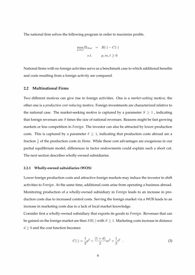
The national firm solves the following program in order to maximize profits.
maxp,m,t
ΠNat = R(·) − C(·)
s.t. p, m, t ≥ 0
National firms with no foreign activities serve as a benchmark case to which additional benefits
and costs resulting from a foreign activity are compared.
2.2 Multinational Firms
Two different motives can give rise to foreign activities. One is a market-seeking motive, the
other one is a production cost-reducing motive. Foreign investments are characterized relative to
the national case. The market-seeking motive is captured by a parameter S ≥ 1 , indicating
that foreign revenues are S times the size of national revenues. Reasons might be fast growing
markets or less competition in Foreign. The investor can also be attracted by lower production
costs. This is captured by a parameter δ ≥ 1, indicating that production costs abroad are a
fraction 1δ of the production costs in Home. While these cost advantages are exogenous in our
partial equilibrium model, differences in factor endowments could explain such a short cut.
The next section describes wholly-owned subsidiaries.
2.2.1 Wholly-owned subsidiaries (WOS)
Lower foreign production costs and attractive foreign markets may induce the investor to shift
activities to Foreign. At the same time, additional costs arise from operating a business abroad.
Monitoring production of a wholly-owned subsidiary in Foreign leads to an increase in pro-
duction costs due to increased control costs. Serving the foreign market via a WOS leads to an
increase in marketing costs due to a lack of local market knowledge.
Consider first a wholly-owned subsidiary that exports its goods to Foreign. Revenues that can
be gained on the foreign market are then SR(·) with S ≥ 1. Marketing costs increase in distance
d ≥ 0 and the cost function becomes
C(·) =1
2p2 +
(1 + d)
2m2 +
1
2t2 . (3)
6
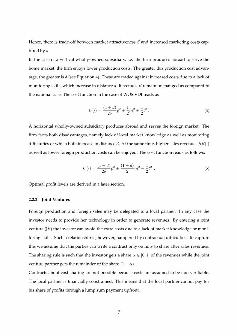
Hence, there is trade-off between market attractiveness S and increased marketing costs cap-
tured by d.
In the case of a vertical wholly-owned subsidiary, i.e. the firm produces abroad to serve the
home market, the firm enjoys lower production costs. The greater this production cost advan-
tage, the greater is δ (see Equation 4). These are traded against increased costs due to a lack of
monitoring skills which increase in distance d. Revenues R remain unchanged as compared to
the national case. The cost function in the case of WOS VDI reads as
C(·) =(1 + d)
2δp2 +
1
2m2 +
1
2t2 . (4)
A horizontal wholly-owned subsidiary produces abroad and serves the foreign market. The
firm faces both disadvantages, namely lack of local market knowledge as well as monitoring
difficulties of which both increase in distance d. At the same time, higher sales revenues SR(·)
as well as lower foreign production costs can be enjoyed. The cost function reads as follows:
C(·) =(1 + d)
2δp2 +
(1 + d)
2m2 +
1
2t2 . (5)
Optimal profit levels are derived in a later section.
2.2.2 Joint Ventures
Foreign production and foreign sales may be delegated to a local partner. In any case the
investor needs to provide her technology in order to generate revenues. By entering a joint
venture (JV) the investor can avoid the extra costs due to a lack of market knowledge or moni-
toring skills. Such a relationship is, however, hampered by contractual difficulties. To capture
this we assume that the parties can write a contract only on how to share after sales revenues.
The sharing rule is such that the investor gets a share α ∈ [0, 1] of the revenues while the joint
venture partner gets the remainder of the share (1 − α).
Contracts about cost sharing are not possible because costs are assumed to be non-verifiable.
The local partner is financially constrained. This means that the local partner cannot pay for
his share of profits through a lump sum payment upfront.
7
We allow for the possibility of technology spillovers in case of joint ventures.8 To capture this
effect, we assume that technology transfers become more expensive if a partner is involved.9
The investor may fear to being imitated by a local partner and to being driven out of business
once she revealed her intangible assets.10 This danger is stronger the weaker institutions and
protection of intellectual property rights are.11 We capture weaker institutions by increasing
distance. Thus technology spillovers are assumed to increase technology costs by the factor
(1 + d).
In order to distinguish the investing firm and the joint venture partner we denote the investor
by superscript 1 and the partner by 2. In the following we describe the payoff structures for JV
Export, JV VDI, and JV HDI.
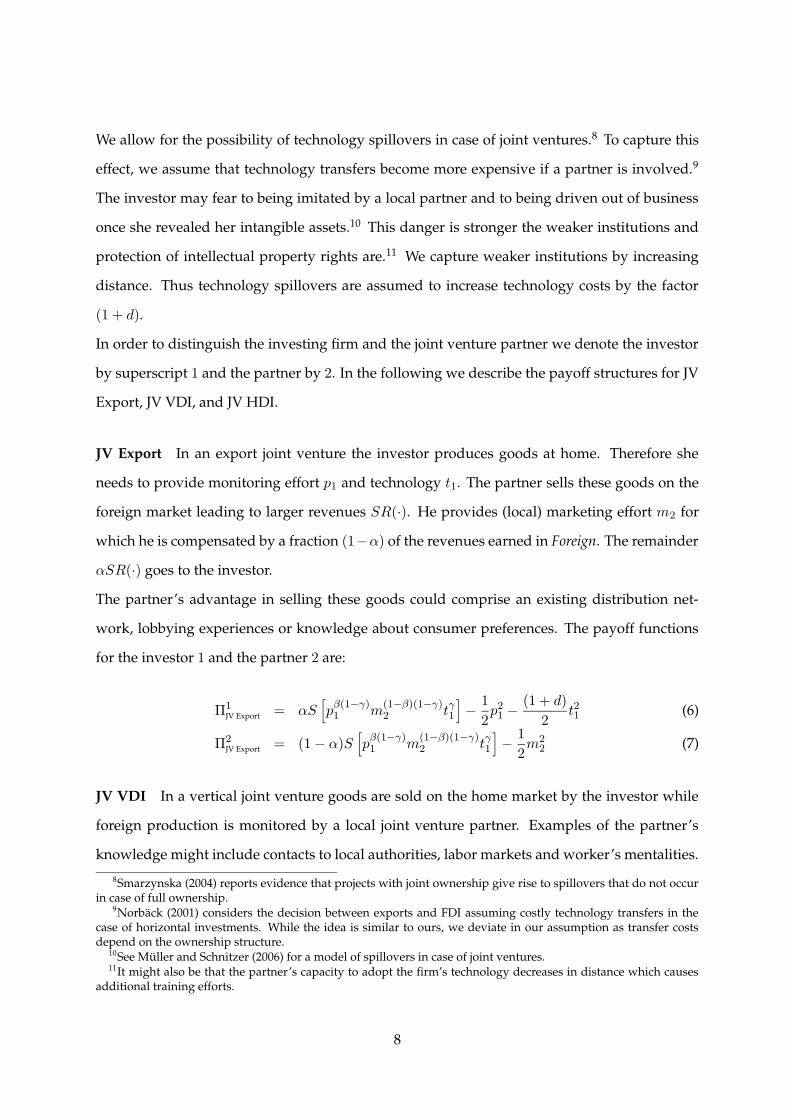
JV Export In an export joint venture the investor produces goods at home. Therefore she
needs to provide monitoring effort p1 and technology t1. The partner sells these goods on the
foreign market leading to larger revenues SR(·). He provides (local) marketing effort m2 for
which he is compensated by a fraction (1−α) of the revenues earned in Foreign. The remainder
αSR(·) goes to the investor.
The partner’s advantage in selling these goods could comprise an existing distribution net-
work, lobbying experiences or knowledge about consumer preferences. The payoff functions
for the investor 1 and the partner 2 are:
Π1JV Export = αS
[
pβ(1−γ)1 m
(1−β)(1−γ)2 tγ1
]
−1
2p21 −
(1 + d)
2t21 (6)
Π2JV Export = (1 − α)S
[
pβ(1−γ)1 m
(1−β)(1−γ)2 tγ1
]
−1
2m2
2 (7)
JV VDI In a vertical joint venture goods are sold on the home market by the investor while
foreign production is monitored by a local joint venture partner. Examples of the partner’s
knowledge might include contacts to local authorities, labor markets and worker’s mentalities.
8Smarzynska (2004) reports evidence that projects with joint ownership give rise to spillovers that do not occurin case of full ownership.
9Norbäck (2001) considers the decision between exports and FDI assuming costly technology transfers in thecase of horizontal investments. While the idea is similar to ours, we deviate in our assumption as transfer costsdepend on the ownership structure.
10See Müller and Schnitzer (2006) for a model of spillovers in case of joint ventures.11It might also be that the partner’s capacity to adopt the firm’s technology decreases in distance which causes
additional training efforts.
8
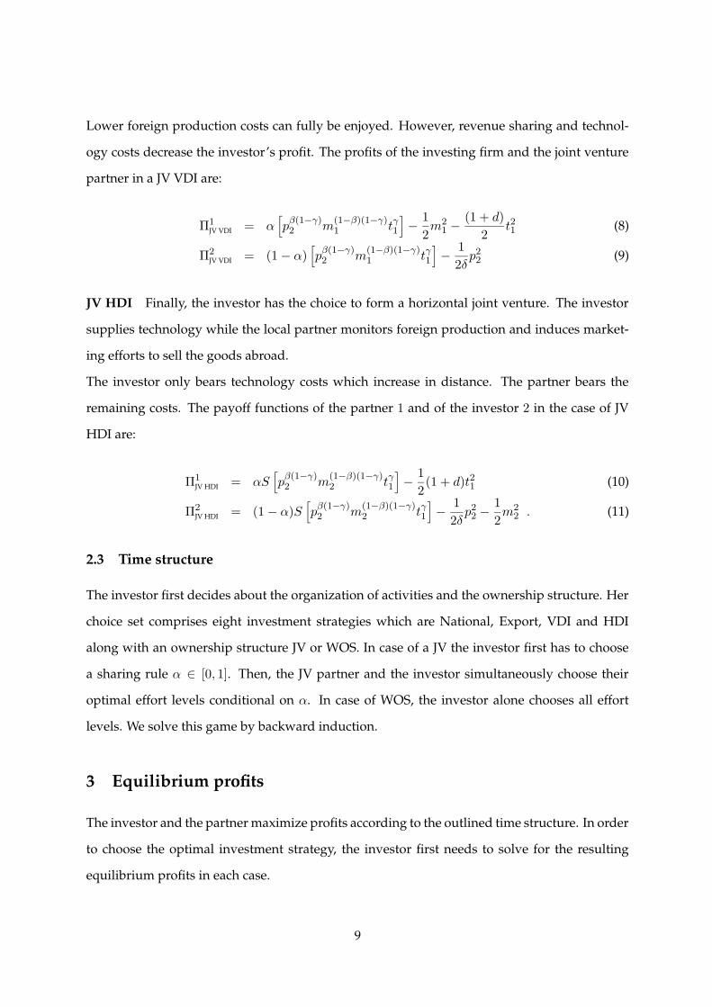
Lower foreign production costs can fully be enjoyed. However, revenue sharing and technol-
ogy costs decrease the investor’s profit. The profits of the investing firm and the joint venture
partner in a JV VDI are:
Π1JV VDI = α
[
pβ(1−γ)2 m
(1−β)(1−γ)1 tγ1
]
−1
2m2
1 −(1 + d)
2t21 (8)
Π2JV VDI = (1 − α)
[
pβ(1−γ)2 m
(1−β)(1−γ)1 tγ1
]
−1
2δp22 (9)
JV HDI Finally, the investor has the choice to form a horizontal joint venture. The investor
supplies technology while the local partner monitors foreign production and induces market-
ing efforts to sell the goods abroad.
The investor only bears technology costs which increase in distance. The partner bears the
remaining costs. The payoff functions of the partner 1 and of the investor 2 in the case of JV
HDI are:
Π1JV HDI = αS
[
pβ(1−γ)2 m
(1−β)(1−γ)2 tγ1
]
−1
2(1 + d)t21 (10)
Π2JV HDI = (1 − α)S
[
pβ(1−γ)2 m
(1−β)(1−γ)2 tγ1
]
−1
2δp22 −
1
2m2
2 . (11)
2.3 Time structure
The investor first decides about the organization of activities and the ownership structure. Her
choice set comprises eight investment strategies which are National, Export, VDI and HDI
along with an ownership structure JV or WOS. In case of a JV the investor first has to choose
a sharing rule α ∈ [0, 1]. Then, the JV partner and the investor simultaneously choose their
optimal effort levels conditional on α. In case of WOS, the investor alone chooses all effort
levels. We solve this game by backward induction.
3 Equilibrium profits
The investor and the partner maximize profits according to the outlined time structure. In order
to choose the optimal investment strategy, the investor first needs to solve for the resulting
equilibrium profits in each case.
9
First, we describe the national case, we then turn to wholly-owned subsidiaries where still no
partner is involved, and last we solve the model for joint ventures.
3.1 National firms
If the investor chooses National she will never enter a joint venture as our model gives no
advantage to national joint ventures that would compensate for resulting agency costs. The
investor chooses p, m, and t to maximize her profits. This results in the following profits,
derived in the appendix.
Π∗Nat =
1
2ββ(1−γ)(1 − β)(1−β)(1−γ)γγ(1 − γ)1−γ (12)
3.2 Wholly-owned subsidiaries
We can solve the investor’s profit maximization problem in the same way as above for the
three cases of WOS Export, WOS VDI, and WOS HDI. We derive the following solutions to
these profit maximization problems.
Π∗WOS Exports = S2
(1
1 + d
)(1−β)(1−γ)
Π∗Nat (13)
Π∗WOS VDI =
(δ
1 + d
)β(1−γ)
Π∗Nat (14)
Π∗WOS HDI = S2δβ(1−γ)
(1
1 + d
)(1−γ)
Π∗Nat (15)
The equilibrium profits reveal the trade-off between additional costs due to distance and for-
eign advantages as expressed by higher sales revenues S and lower production costs δ.
The choices whether to serve the foreign market and whether to produce abroad can be sep-
arated in our model. The reason is that we do not assume any costs of fragmentation as it is
sometimes done in the literature. Costs of fragmentation occur if splitting up production steps
causes additional costs that would not arise if all activities are kept at one place.
The production and the sales decision differ with respect to their sector dependence. Consider
first the decision which market to serve. All sectors benefit from higher sales revenues abroad.
Marketing-intensive sectors suffer more from a lack of local market knowledge as this activity
10
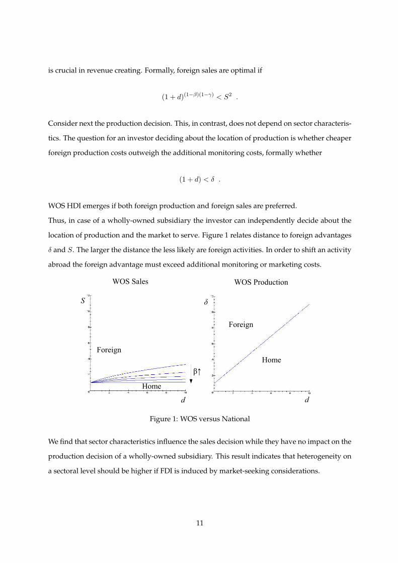
is crucial in revenue creating. Formally, foreign sales are optimal if
(1 + d)(1−β)(1−γ) < S2 .
Consider next the production decision. This, in contrast, does not depend on sector characteris-
tics. The question for an investor deciding about the location of production is whether cheaper
foreign production costs outweigh the additional monitoring costs, formally whether
(1 + d) < δ .
WOS HDI emerges if both foreign production and foreign sales are preferred.
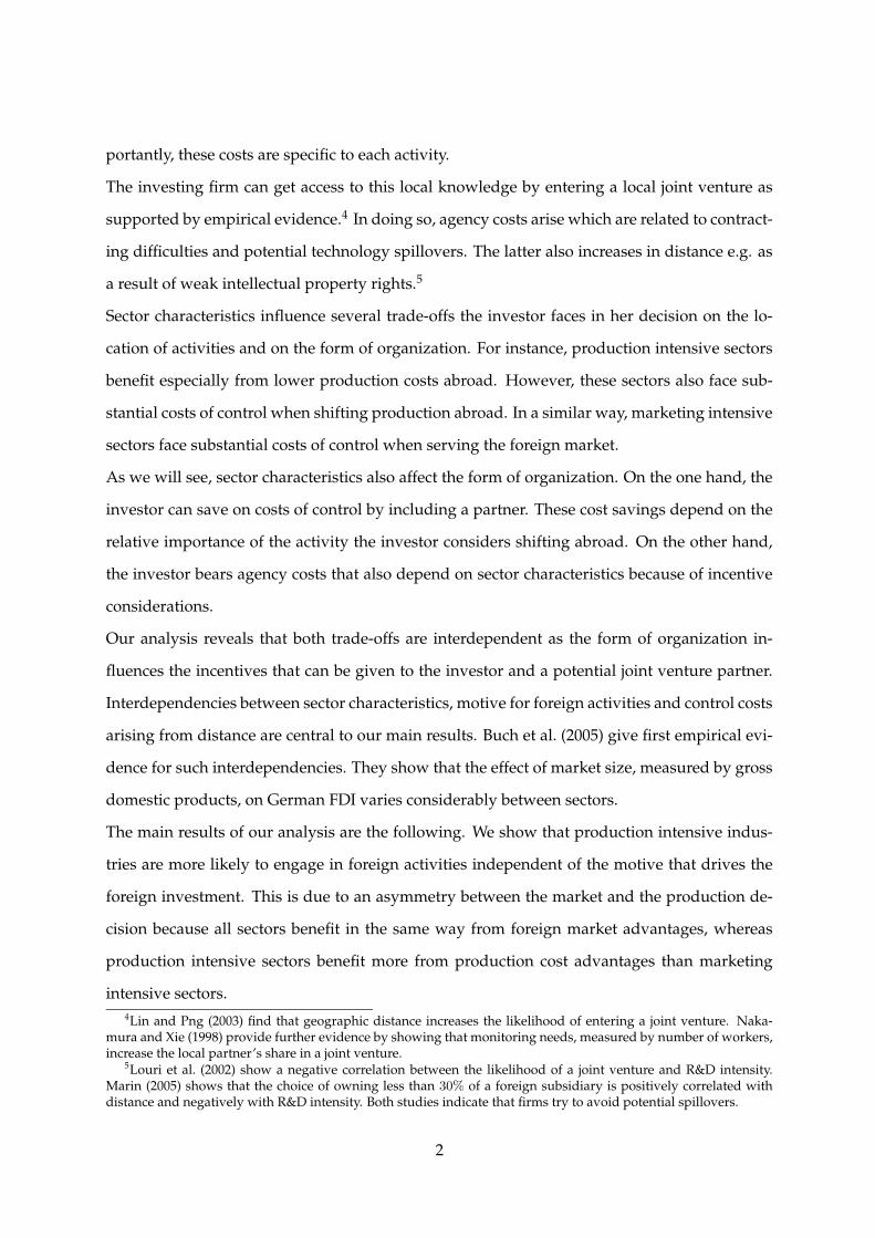
Thus, in case of a wholly-owned subsidiary the investor can independently decide about the
location of production and the market to serve. Figure 1 relates distance to foreign advantages
δ and S. The larger the distance the less likely are foreign activities. In order to shift an activity
abroad the foreign advantage must exceed additional monitoring or marketing costs.
Figure 1: WOS versus National
We find that sector characteristics influence the sales decision while they have no impact on the
production decision of a wholly-owned subsidiary. This result indicates that heterogeneity on
a sectoral level should be higher if FDI is induced by market-seeking considerations.
11
3.3 Joint ventures
In case of a joint venture, both investor and partner simultaneously choose their effort levels in
order to maximize their profits, given the sharing rule α. Anticipating these equilibrium profits
the investor chooses α such as to maximize her profits. In the appendix we derive the solutions
for the following three cases.
JV Export Suppose the investor chooses to sell goods in Foreign via a joint venture partner.
The investor’s optimal share of revenues α∗ is then given by Equation 16.
α∗JV Export =
1 + γ + β(1 − γ)
2(16)
The investor’s share increases in the importance of the provided inputs, namely in the impor-
tance of technology γ and of production β(1−γ). To put it differently, the more important is the
marketing activity, the higher is the share of the local joint venture partner in order to provide
efficient incentives.
The investor’s profit in the case of JV Export is:
Π1∗JV Export =
1
4S2(
1
1 + d)γ(1 + (1 − β)(1 − γ))
((1 − β)(1 − γ))(1−β)(1−γ)(2 − (1 − β)(1 − γ))2−(1−β)(1−γ)Π∗Nat (17)
JV Export profits are characterized by a trade-off between the foreign market attractiveness
S on the one hand and additional costs due to spillovers(
11+d
)γand revenue sharing on the
other.
JV VDI If the investor opts for JV VDI the partner supplies production inputs while the in-
vestor provides technology and marketing effort. Goods are sold on the home market. The
optimal share α∗V DI turns out to be lowest when production is the most important import fac-
tor.
α∗JV VDI =
2 − β(1 − γ)
2(18)
12
The result resembles that of JV Export. While the optimal share α∗JV Export increases in the impor-
tance of production β(1 − γ) the optimal share α∗JV VDI increases in the importance of marketing
(1 − β). In both cases the effect of technology γ increases the investor’s participation. In short,
the importance of the provided input factor increases the respective parties revenue share.
13
Knowing the efficient share of sales revenues we can derive the investor’s profit in case of JV
VDI:
Π1∗JV VDI =
1
4
(1
1 + d
)γ
(δβ(1 − γ))β(1−γ)
(1 + β(1 − γ)) (2 − β(1 − γ))2−β(1−γ)Π∗Nat (19)
As one would expect lower foreign production costs increase profits. This cost effect is more
pronounced in production intensive sectors.
JV HDI The investor only provides technology in a JV HDI. The partner monitors production
and also sells the goods on the foreign market. Solving for the optimal revenue share left to the
investor leads to Equation 20.
α∗JV HDI =
1 + γ
2(20)
The optimal share does not depend on β as both production and marketing are in the partner’s
hands. However, technology influences the investor’s decision as technology is the intangible
asset the partner cannot contribute. If technology does not play a role, formally if γ approaches
zero, the optimal share is 1/2.
Π1∗JV HDI =
1
4S2δβ(1−γ)
(1
1 + d
)γ
(2 − γ) (1 + γ)1+γ(1 − γ)2(1−γ)Π∗Nat (21)
The profit function already points at some results of the model. First, foreign market advan-
tages accrue to all sectors while the magnitude of cost savings due to foreign production de-
pend on production intensity. Second, technology spillovers decrease the profits made by the
investor in all joint ventures. The effect is higher in high technology sectors, i.e. if γ is high,
and in distant countries, i.e. if d is high.
If we ignore technology for a moment Equation (21) boils down to
Π1∗JV HDI =
1
2S2δβΠ∗
Nat .
In that case the investor only receives half of the profits, this reflects the agency costs due
to partnership, but the foreign advantages increase profits by S2 and δβ . Technology further
14
reduces the investor’s profits as spillovers occur. Additionally, an inefficiency arises as only
the investor can provide technology. Hence, incentives are split between the investor and the
partner. A fact that further reduces investor’s profits.
4 Optimal investment strategy
So far we described the equilibrium profits of the investing firm for the different investment
choices. We can now ask which is the firm’s best choice depending on the business environment
it faces. The results focus on the influence of distance. We start with investigating internation-
alization strategies when the firm exploits lower production costs or develops a foreign market.
In the last part of the analysis we look at high technology sectors.
The firm takes the market attractiveness, production cost differences and distance as given.
Furthermore, the firm operates in a certain sector. These exogenous parameters determine the
firm’s best choice.
4.1 Production cost effects
Consider a firm which faces lower foreign production costs and gains the same revenues in
Home and Foreign. The only force driving the investor to shift activities abroad is the produc-
tion cost effect δ.12 Abstract further from technology inputs to focus on agency costs due to
contractual limitations.
Result 1 summarizes the main effects that are spurred by the cost-reducing motive of the firm
in low technology industries. Parameters referring to production cost advantages are indicated
by tilde. Proofs are given in the appendix.
Result 1 Impact of production cost advantage for low tech goods
(i) There exists a critical production cost advantage δ such that for δ < δ production takes place
at home and for δ > δ production takes place abroad. The critical δ increases in distance and
decreases in β.
(ii) If the investor prefers to produce at home the good is sold at home as well.
12Braconier et al. (2005) support vertical motives of multinational activities. They find that more FDI takes placein countries where unskilled labor is relatively cheap.
15
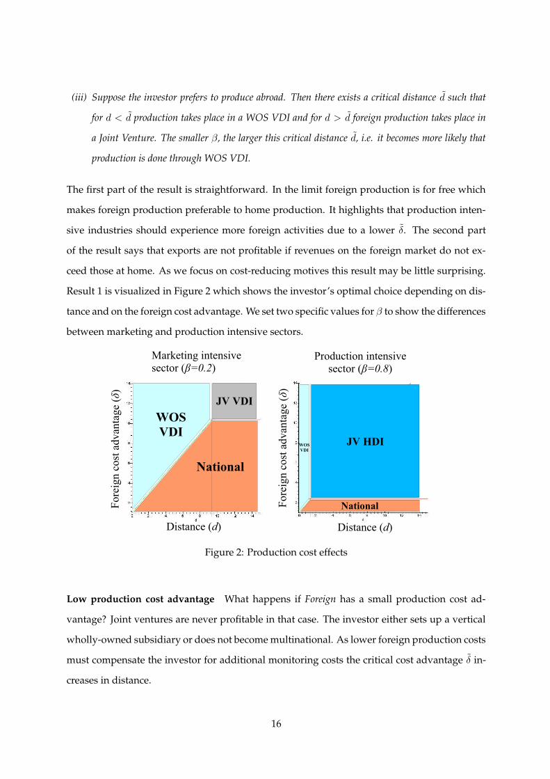
(iii) Suppose the investor prefers to produce abroad. Then there exists a critical distance d such that
for d < d production takes place in a WOS VDI and for d > d foreign production takes place in
a Joint Venture. The smaller β, the larger this critical distance d, i.e. it becomes more likely that
production is done through WOS VDI.
The first part of the result is straightforward. In the limit foreign production is for free which
makes foreign production preferable to home production. It highlights that production inten-
sive industries should experience more foreign activities due to a lower δ. The second part
of the result says that exports are not profitable if revenues on the foreign market do not ex-
ceed those at home. As we focus on cost-reducing motives this result may be little surprising.
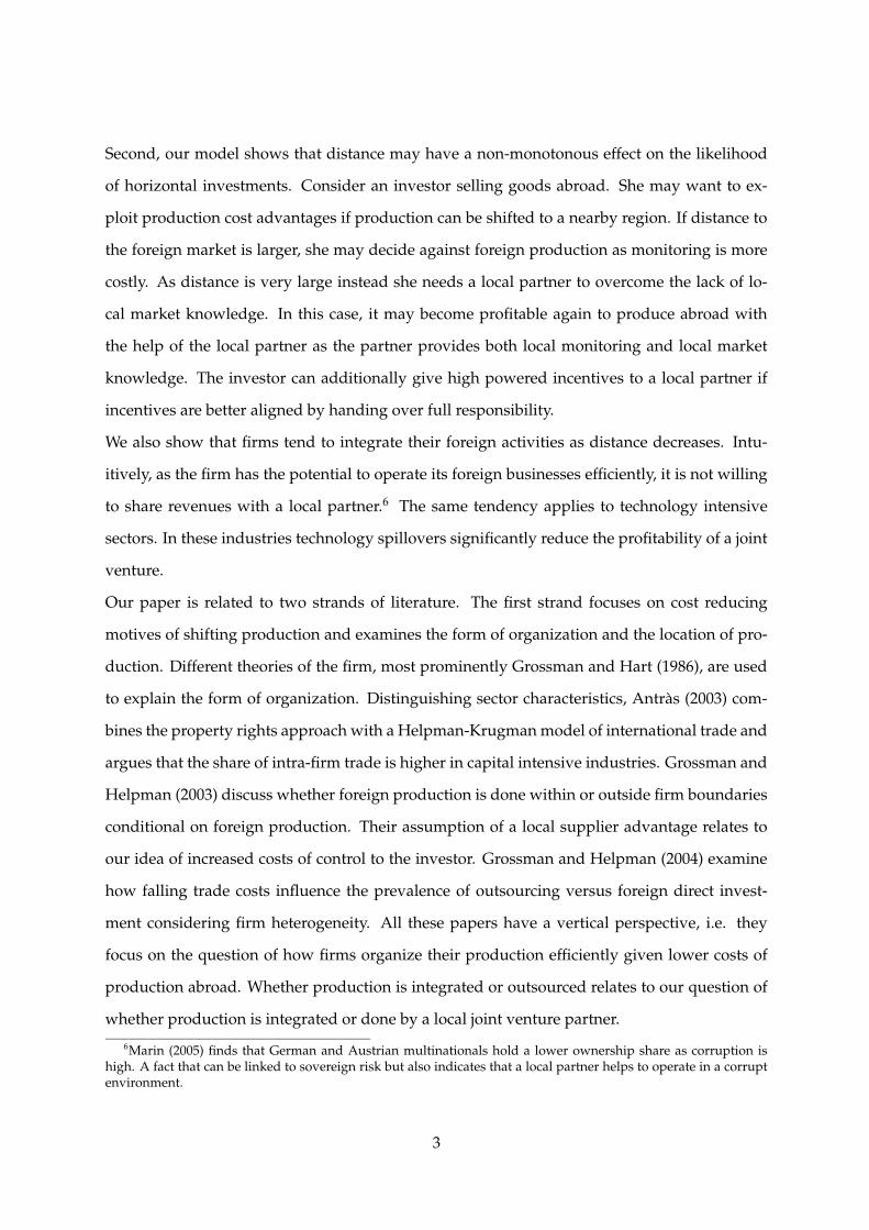
Result 1 is visualized in Figure 2 which shows the investor’s optimal choice depending on dis-
tance and on the foreign cost advantage. We set two specific values for β to show the differences
between marketing and production intensive sectors.
Figure 2: Production cost effects
Low production cost advantage What happens if Foreign has a small production cost ad-
vantage? Joint ventures are never profitable in that case. The investor either sets up a vertical
wholly-owned subsidiary or does not become multinational. As lower foreign production costs
must compensate the investor for additional monitoring costs the critical cost advantage δ in-
creases in distance.
16
High production cost advantage What happens if the foreign cost advantage is large? As
shown in Result 1 foreign production is then always profitable. For short distances WOS VDI
is the best strategy. For large distances the investor enters a joint venture. The reason is that
the investor’s monitoring costs increase in distance. Hence, distance also increases the value
of the partner’s local knowledge. As a consequence, entering a partnership pays more as the
investor saves on control costs. To put it differently, agency costs do not increase in distance
d while the investor’s monitoring costs do. The threshold level that separates WOS VDI from
joint ventures is named d.
Sector differences How do production and marketing intensive sectors differ? First, the more
production intensive a good, the wider is the parameter range that leads to foreign production.
The reason is that the magnitude of cost reduction is greater if production is important in rev-
enue creating. Recall that in case of a WOS the decision to produce abroad does not depend
on industry characteristics because the investor’s monitoring costs increase side by side with
the cost advantage. This is different in a JV, as production intensive joint ventures benefit from
lower production costs while no additional monitoring costs arise.
Sector differences also influence the choice of JV HDI versus JV VDI. Surprisingly, foreign sales
can be optimal even if there is no market advantage. We state this observation in Lemma 1.
Lemma 1 Suppose the investor considers to produce abroad through a Joint Venture. Then there exists
a critical β such that for any β < β the investor prefers a VDI Joint Venture, and for β > β she prefers
a HDI Joint Venture.
The reason is an inefficiency that arises if incentives are split between the investor and the local
partner. To get a better intuition for Lemma 1 consider a situation in which JV VDI is optimal.
Increasing the production intensity of the revenue generating process leads to an increase of the
partner’s share to provide appropriate incentives. At the same time the relevance of marketing
declines. At a point little extra is needed if the partner also sells the goods on the foreign
market. As soon as the efficiency gain from bundling incentives at the partner’s side outweighs
this additional share JV HDI are optimal. Incentives are then best aligned as the joint venture
partner is responsible not only for production but also for sales.
Serving a foreign market might be not valuable in form of a wholly-owned subsidiary. How-
17
ever, if the multinational firm already bears the costs stemming from a joint venture it might
find serving the foreign market attractive - through the hands of the partner. This situation
is more likely as the sector is production intensive. Formally, JV HDI dominates JV VDI if
production intensity is above β which can approximated by β ≈ 0.4471.
In summary, the production cost-reducing motive renders joint ventures that are production
intensive more profitable. Intuitively, the agency costs of a joint venture are more easily recov-
ered as the cost savings are substantial. Agency costs are not recovered if the foreign advantage
is relatively small. Furthermore, joint ventures occur if distance is relatively large as distance
corresponds to the partner’s specific advantage. Once JV is optimal distance does not influence
the investor’s profits. This is not the case for WOS VDI. In that case distance reflects increased
monitoring costs that decrease profits. This channel complements trade costs that are usually
thought of to decrease the likelihood of vertical foreign direct investments. Finally, we see that
the relative importance of an activity joint with the motive for foreign activities determines the
investor’s optimal choice.
4.2 Market advantage effects
Market-seeking is found to be another reason for companies to become multinational, reflected
by the fact that most foreign direct investments take place between developed countries. Em-
pirically, Head and Mayer (2004) show that a ten percent increase in market potential increases
the probability of a European region to be chosen by a Japanese investor between three and
eleven per cent. In the theoretical literature, monopolistic competition combined with a love
for variety is proposed as one rationale for why firms would serve foreign markets. Strategic
decisions are frequently cited in newspapers when firms promote their expansion strategies.
First mover advantages and expected market growth might underlie such ’strategic decisions’.
We capture foreign market attractiveness by a parameter S ≥ 1, without investigating in detail
the underlying factors.13 In that way we translate the market-seeking motive of a firm into S
times National revenues R that can be gained abroad as opposed to home.
The effects of higher sales revenues differ from production cost effects as the market advantage
13The foreign market might also be less attractive in terms of revenues. However, in this case there is no reasonfor the investor to invest abroad. Hence, we restrict our attention to S ≥ 1 as the relevant cases when foreignactivities occur.
18
affects total sales revenues independent of sector characteristics. We start by exploring the
optimal investment strategies under the assumption of equal production costs in Home and
Foreign, abstracting from technology inputs.
The following result summarizes how the market-seeking motive affects the investor’s optimal
investment strategy in low technology sectors. Parameters referring to foreign market advan-
tages are indicated by hat.
Result 2 Impact of foreign market advantage for low tech goods
(i) There exists a critical size of the foreign market, S ≤√
2, such that for S < S, the product is sold
on the home market and for S > S, the product is sold in foreign.
The critical S increases in d and it decreases in β. That is, the smaller the distance or the less
marketing intensive the production the smaller the foreign market advantage needs to be for the
investor to prefer selling abroad.
(ii) If the investor serves the domestic market the good is produced in home.
(iii) Suppose the investor prefers to serve the foreign market. Then there exists a critical distance d
such that for d < d the foreign market is served through WOS Exports and for d > d the foreign
market is served through a Joint Venture. The larger β, the larger this critical distance d, i.e. the
more likely is it that the foreign market is served through WOS Exports.
As in the case of production cost advantages we find a critical foreign advantage S at which
the investor is indifferent between national and multinational activities. The additional costs
of foreign activities equal the additional revenues at these points. The costs depend on the
mode of organization. Wholly-owned subsidiaries suffer from lacking market knowledge, joint
ventures cause agency costs. Vertical FDI are never profitable as there is no benefit of operating
a foreign business but costs.
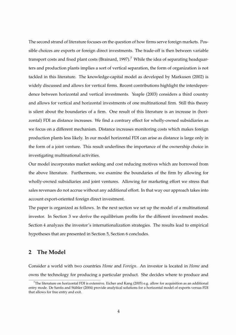
Figure 3 illustrates the optimal strategy of a multinational firm as the market attractiveness
of foreign S increases. The graph shows two goods, one intensive in production, the other
intensive in marketing to visualize sector differences that are presented in the following. Next,
we look at situations in which foreign market attractiveness is low.
19
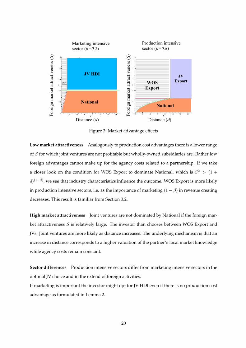
Figure 3: Market advantage effects
Low market attractiveness Analogously to production cost advantages there is a lower range
of S for which joint ventures are not profitable but wholly-owned subsidiaries are. Rather low
foreign advantages cannot make up for the agency costs related to a partnership. If we take
a closer look on the condition for WOS Export to dominate National, which is S2 > (1 +
d)(1−β), we see that industry characteristics influence the outcome. WOS Export is more likely
in production intensive sectors, i.e. as the importance of marketing (1 − β) in revenue creating
decreases. This result is familiar from Section 3.2.
High market attractiveness Joint ventures are not dominated by National if the foreign mar-
ket attractiveness S is relatively large. The investor than chooses between WOS Export and
JVs. Joint ventures are more likely as distance increases. The underlying mechanism is that an
increase in distance corresponds to a higher valuation of the partner’s local market knowledge
while agency costs remain constant.
Sector differences Production intensive sectors differ from marketing intensive sectors in the
optimal JV choice and in the extend of foreign activities.
If marketing is important the investor might opt for JV HDI even if there is no production cost
advantage as formulated in Lemma 2.
20
Lemma 2 Suppose the investor considers to serve the foreign market through a Joint Venture. Then
there exists a critical β such that for any β < β the investor prefers a Horizontal JV, and for β > β he
prefers an Export JV.
By a similar reasoning as in the case of production cost advantages the investor might shift
production abroad to bundle incentives at the partner’s side. The critical importance of pro-
duction is numerically approximated by β ≈ 0.5529. Below this value JV HDI dominates JV
Export. Above this value the investor benefits more from keeping control over the production
process.
How can we explain this result? Consider a situation in which JV Export is optimal, i.e. distance
together with foreign market attractiveness is relatively large. However, the investor produces
in Home as the additional share a partner would require to induce production effort is too high.
An increase of the marketing intensity (1 − β) leads to high powered incentives given to the
joint venture partner. Hence, additional incentives to provide production monitoring activities
are low. At the same time there is an efficiency gain as incentives are bundled in the hands of
one party. For this reason production is shifted abroad handing over the full responsibility of
all revenue creating activities to the partner.
The trade-off exists between bundling incentives and keeping control over crucial activities.
The former increases overall profits, the latter avoids relatively costly incentives given to the
partner in form of a high share (1 − α).
Sectors also differ in their extend of foreign activities. As marketing intensity increases one
might expect more foreign activities if market-seeking is the motive for the firm’s foreign ac-
tivities. But Result 2 tells the opposite story. The reason is that all sectors benefit from higher
sales revenues S while additional weight is put on the investor’s disadvantage as marketing is
important. This additional weight renders foreign activities less profitable.
Up to this point we found two results that are independent of whether the investor develops a
foreign market or whether she seeks to save on production costs. First, joint ventures are more
likely if distance is large as distance reflects the value of a partner’s local knowledge. Using
data on U.S. multinational firms Desai et al. (2004) show that partial ownership has declined
between 1982 and 1997. Thinking of economic integration as a process of reducing foreign costs
of control our model provides one theoretical explanation for such a development.
21
Second, foreign activities are more likely in production intensive industries. These industries
have two advantages as compared to marketing intensive ones. The relative importance of
the production process results in high cost-savings if production is shifted abroad. As argued
before, the cost savings are particular to the production process. The relative unimportance of
sales activities results in low additional costs of control if the foreign market is served while
the full market advantage can be enjoyed.
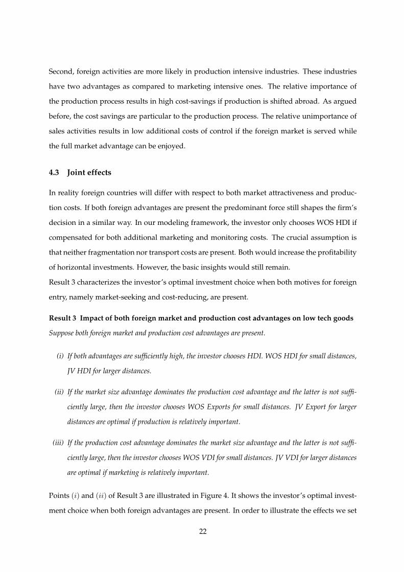
4.3 Joint effects
In reality foreign countries will differ with respect to both market attractiveness and produc-
tion costs. If both foreign advantages are present the predominant force still shapes the firm’s
decision in a similar way. In our modeling framework, the investor only chooses WOS HDI if
compensated for both additional marketing and monitoring costs. The crucial assumption is
that neither fragmentation nor transport costs are present. Both would increase the profitability
of horizontal investments. However, the basic insights would still remain.
Result 3 characterizes the investor’s optimal investment choice when both motives for foreign
entry, namely market-seeking and cost-reducing, are present.
Result 3 Impact of both foreign market and production cost advantages on low tech goods
Suppose both foreign market and production cost advantages are present.
(i) If both advantages are sufficiently high, the investor chooses HDI. WOS HDI for small distances,
JV HDI for larger distances.
(ii) If the market size advantage dominates the production cost advantage and the latter is not suffi-
ciently large, then the investor chooses WOS Exports for small distances. JV Export for larger
distances are optimal if production is relatively important.
(iii) If the production cost advantage dominates the market size advantage and the latter is not suffi-
ciently large, then the investor chooses WOS VDI for small distances. JV VDI for larger distances
are optimal if marketing is relatively important.
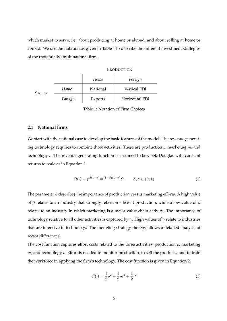
Points (i) and (ii) of Result 3 are illustrated in Figure 4. It shows the investor’s optimal invest-
ment choice when both foreign advantages are present. In order to illustrate the effects we set
22
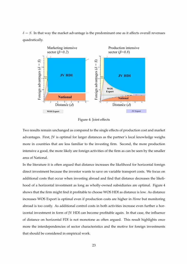
δ = S. In that way the market advantage is the predominant one as it affects overall revenues
quadratically.
Figure 4: Joint effects
Two results remain unchanged as compared to the single effects of production cost and market
advantages. First, JV is optimal for larger distances as the partner’s local knowledge weighs
more in countries that are less familiar to the investing firm. Second, the more production
intensive a good, the more likely are foreign activities of the firm as can be seen by the smaller
area of National.
In the literature it is often argued that distance increases the likelihood for horizontal foreign
direct investment because the investor wants to save on variable transport costs. We focus on
additional costs that occur when investing abroad and find that distance decreases the likeli-
hood of a horizontal investment as long as wholly-owned subsidiaries are optimal. Figure 4
shows that the firm might find it profitable to choose WOS HDI as distance is low. As distance
increases WOS Export is optimal even if production costs are higher in Home but monitoring
abroad is too costly. As additional control costs in both activities increase even further a hor-
izontal investment in form of JV HDI can become profitable again. In that case, the influence
of distance on horizontal FDI is not monotone as often argued. This result highlights once
more the interdependencies of sector characteristics and the motive for foreign investments
that should be considered in empirical work.
23
4.4 Technology
Do technology intensive sectors differ in their internationalization strategies? This question
is answered in this last part of the analysis. In general, technology makes joint ventures less
profitable as spillovers are costly. Furthermore, foreign activities are less likely as distance
increases. So far, a joint venture could overcome all hurdles related to distance. But if tech-
nology is relevant in revenue generating joint ventures are hampered by distance, too. In this
case, distance describes the firm’s capacity to transfer technology and to protect its proprietary
knowledge. A second effect is that incentives are naturally split between the investor and the
partner which constitutes an additional inefficiency. Consequently, national firms as well as
wholly-owned subsidiaries are chosen for a wider range of parameters as γ increases. If the
weight on technology γ exceeds the one on the remaining activities (1 − γ) a joint venture is
never profitable. The reason is that we assume distance to affect technology costs in the same
way as marketing or monitoring costs. This assumption eases the illustration of the result but
could easily be relaxed.
Result 4 Impact of technology on investment decision
(i) The critical distances d and d above which joint ventures are preferred over wholly-owned subsidiaries
increases in the importance of technology γ of an industry making full ownership more likely.
(ii) As the importance of technology γ in revenue creating increases joint ventures become less attractive
as compared to National.
(iii) If technology is the major revenue creating input, i.e. if γ > 0.5 the firm never enters a joint venture.
(iv) The ownership share of the investor α in a joint venture increases as technology becomes more im-
portant in revenue creating, i.e. as γ increases.
The results predict that the ownership of an investor increases as technology intensity increases.
Two effects lead to the result. Wholly-owned subsidiaries become a preferred ownership struc-
ture. Plus, conditional on joint ventures the investor’s share α∗ increases as technology be-
comes more important.
24
5 Empirical hypotheses
Our model gives rise to several empirical hypotheses. The aim is to provide testable predictions
that can be confronted with the data.
Desai et al. (2004) conclude that the forces of globalization lead to more integration. Thinking
of globalization as reducing distance our first hypothesis relates to their general statement.
Hypothesis 1 Foreign investments that are situated in countries that are close in terms of geographic
distance, culture and institutions, i.e. countries that display a low distance d, are more likely to be
organized as wholly-owned subsidiaries.
The investor’s potential to control and operate foreign activities is assumed to decrease in dis-
tance. Reversely, the value of local knowledge increases in distance. Hypothesis 2 relates to
this mechanism.
Hypothesis 2 As the distance d between an investing firm and the host country increases, it is more
likely that a joint venture is the preferred investment mode.
At the same time, technology spillovers decrease the profitability of joint ventures. For this
reason we describe the link between distance and joint ventures more precisely.
Hypothesis 3 Less joint ventures appear as high technology sectors are considered, i.e. as the weight
on technology γ increases.
We have seen that sectoral differences play an important role for the understanding of multi-
national activities. This is captured by the following hypotheses.
Hypothesis 4 Production intensive sectors are more likely to operate a foreign business, independent
of the investment motive.
Production intensive and marketing intensive industries react in opposite ways as the choice
of JV HDI is considered. Marketing intensive industries prefer JV HDI if market attractiveness
is the motive for foreign activities. Production intensive industries prefer JV HDI when the
production cost advantage is the motive for foreign activities. The next hypothesis generalizes
this observation.
25
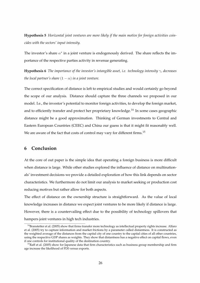
Hypothesis 5 Horizontal joint ventures are more likely if the main motive for foreign activities coin-
cides with the sectors’ input intensity.
The investor’s share α∗ in a joint venture is endogenously derived. The share reflects the im-
portance of the respective parties activity in revenue generating.
Hypothesis 6 The importance of the investor’s intangible asset, i.e. technology intensity γ, decreases
the local partner’s share (1 − α) in a joint venture.
The correct specification of distance is left to empirical studies and would certainly go beyond
the scope of our analysis. Distance should capture the three channels we proposed in our
model. I.e., the investor’s potential to monitor foreign activities, to develop the foreign market,
and to efficiently transfer and protect her proprietary knowledge.14 In some cases geographic
distance might be a good approximation. Thinking of German investments to Central and
Eastern European Countries (CEEC) and China our guess is that it might fit reasonably well.
We are aware of the fact that costs of control may vary for different firms.15
6 Conclusion
At the core of out paper is the simple idea that operating a foreign business is more difficult
when distance is large. While other studies explored the influence of distance on multination-
als’ investment decisions we provide a detailed exploration of how this link depends on sector
characteristics. We furthermore do not limit our analysis to market seeking or production cost
reducing motives but rather allow for both aspects.
The effect of distance on the ownership structure is straightforward. As the value of local
knowledge increases in distance we expect joint ventures to be more likely if distance is large.
However, there is a countervailing effect due to the possibility of technology spillovers that
hampers joint ventures in high tech industries.
14Branstetter et al. (2005) show that firms transfer more technology as intellectual property rights increase. Alfaroet al. (2005) try to capture information and market frictions by a parameter called distantness. It is constructed asthe weighted average of the distances from the capital city of one country to the capital cities of all other countries,using the respective GDP shares as weights. They show that distantness has a negative effect on capital flows, evenif one controls for institutional quality of the destination country.
15Raff et al. (2005) show for Japanese data that firm characteristics such as business group membership and firmage increase the likelihood of FDI versus exports.
26
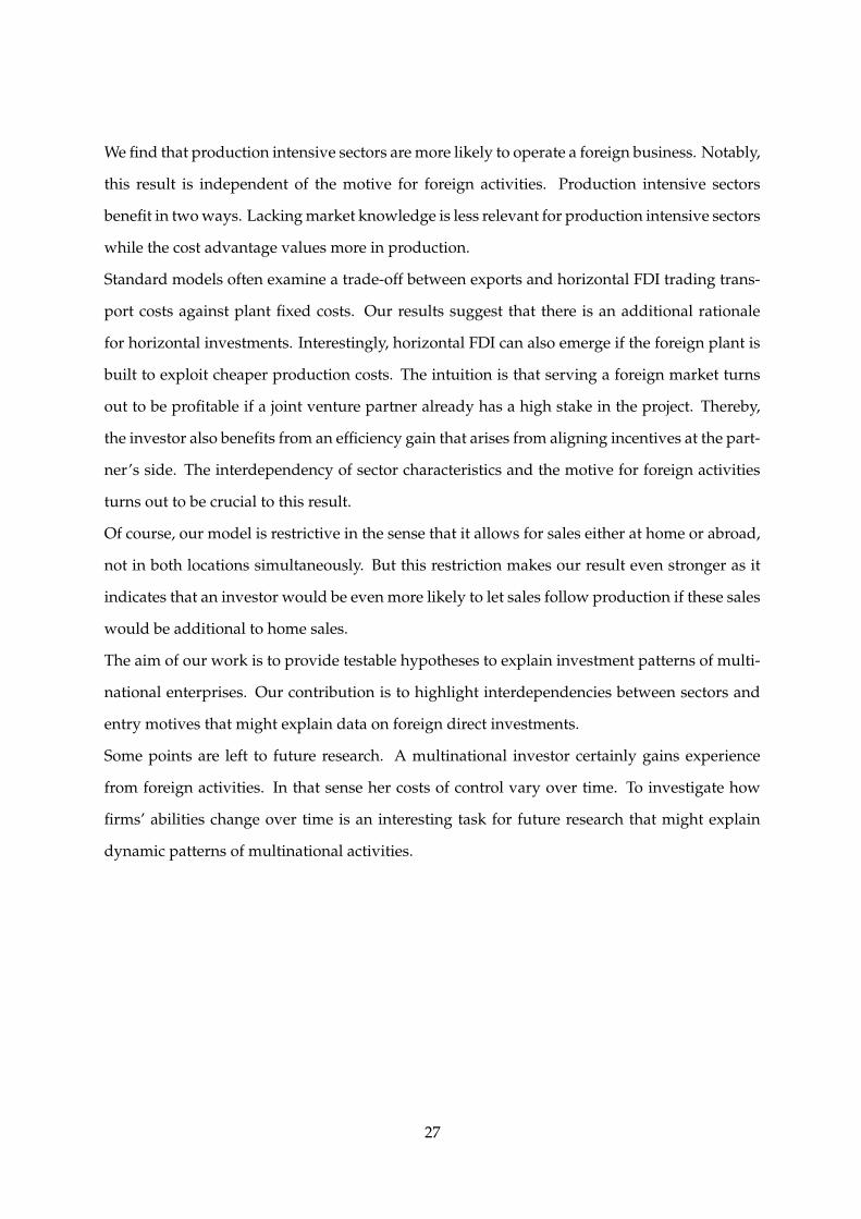
We find that production intensive sectors are more likely to operate a foreign business. Notably,
this result is independent of the motive for foreign activities. Production intensive sectors
benefit in two ways. Lacking market knowledge is less relevant for production intensive sectors
while the cost advantage values more in production.
Standard models often examine a trade-off between exports and horizontal FDI trading trans-
port costs against plant fixed costs. Our results suggest that there is an additional rationale
for horizontal investments. Interestingly, horizontal FDI can also emerge if the foreign plant is
built to exploit cheaper production costs. The intuition is that serving a foreign market turns
out to be profitable if a joint venture partner already has a high stake in the project. Thereby,
the investor also benefits from an efficiency gain that arises from aligning incentives at the part-
ner’s side. The interdependency of sector characteristics and the motive for foreign activities
turns out to be crucial to this result.
Of course, our model is restrictive in the sense that it allows for sales either at home or abroad,
not in both locations simultaneously. But this restriction makes our result even stronger as it
indicates that an investor would be even more likely to let sales follow production if these sales
would be additional to home sales.
The aim of our work is to provide testable hypotheses to explain investment patterns of multi-
national enterprises. Our contribution is to highlight interdependencies between sectors and
entry motives that might explain data on foreign direct investments.
Some points are left to future research. A multinational investor certainly gains experience
from foreign activities. In that sense her costs of control vary over time. To investigate how
firms’ abilities change over time is an interesting task for future research that might explain
dynamic patterns of multinational activities.
27
References
Alfaro, L., Kalemli-Ozcan, S., and Volosovych, V. (2005). Capital flows in a globalized world: The role
of policies and institutions. NBER Working Paper No. 11696.
Antràs, P. (2003). Firms, contracts, and trade structure. Quarterly Journal of Economics, 118(4):1375–
1418.
Braconier, H., Norbäck, P.-J., and Urban, D. (2005). Multinational enterprises and wage costs. Journal
of International Economics, 67(2):446–470.
Brainard, S. L. (1997). An empirical assessment of the proximity-concentration trade-off between
multinational sales and trade. American Economic Review, 87(4):520–544.
Branstetter, L., Fisman, R., and Foley, C. F. (2005). Do stronger intellectual property rights increase
international technology transfer? Empirical evidence from U.S. firm level data. NBER Working Paper
No. 11516.
Buch, C. M., Kleinert, J., Lipponer, A., and Toubal, F. (2005). Determinants and effects of foreign direct
investment: evidence from german firm-level data. Economic Policy, 20(41):52–110.
De Santis, R. A. and Stähler, F. (2004). Endogenous market structures and the gains from foreign direct
investment. Journal of International Economics, 64(2):545–565.
Desai, M. A., Foley, C. F., and Hines, Jr, J. R. (2004). The costs of shared ownership: Evidence from
international joint ventures. Journal of Financial Economics, 73(2):323–374.
Eicher, T. and Kang, J. W. (2005). Trade, foreign direct investment or acquisition: Optimal entry modes
for multinationals. Journal of Development Economics, 77(1):207–228.
Grossman, G. M. and Helpman, E. (2003). Outsourcing versus fdi in industry equilibrium. Journal of
the European Economic Association, 1(2-3):317–327.
Grossman, G. M. and Helpman, E. (2004). Managerial incentives and the international organization
of production. Journal of International Economics, 63:237–262.
Grossman, S. J. and Hart, O. D. (1986). The costs and benefits of ownership: A theory of vertical and
lateral integration. The Journal of Political Economy, 94(4):691–719.
Hanson, G. H., Mataloni, jr, R. J., and Slaughter, M. J. (2003). Vertical production networks in multi-
national firms. NBER Working Paper No. 9723.
28
Head, K. and Mayer, T. (2004). Market potential and the location of japanese investment in the euro-
pean union. Review of Economics and Statistics, 86(4):959–972.
Hummels, D., Ishii, J., and Yi, K.-M. (2001). The nature and growth of vertical specialization in world
trade. Journal of International Economics, 54(1):75–96.
Lin, C.-C. S. and Png, I. (2003). Monitoring costs and the mode of international investment. Journal of
Economic Geography, 3(3):261 – 274.
Louri, H., Loufir, R., and Papanastassiou, M. (2002). Foreign investment and ownership structure: An
empirical analysis. Empirica, 29:31–45.
Marin, D. (2005). A new international division of labor in europe: Outsourcing and offshoring to
eastern europe. Munich Economics - Discussion paper, 17.
Markusen, J. R. (2002). Multinational firms and the theory of international trade. The MIT press.
Müller, T. and Schnitzer, M. (2006). Technology transfer and spillovers in international joint ventures.
Journal of International Economics, forthcoming.
Nakamura, M. and Xie, J. (1998). Nonverifiability, noncontractability and ownership determination
models in foreign direct investment, with an application to foreign operations in japan. International
Journal of Industrial Organization, 16:571–599.
Norbäck, P.-J. (2001). Multinational firms, technology and location. Journal of International Economics,
2(54):449–469.
Raff, H., Ryan, M., and Stähler, F. (2005). Asset ownership and foreign-market entry. CESifo Working
Paper No. 1676.
Rauch, J. E. (2001). Business and social networks in international trade. Journal of Economic Literature,
39(4):1177–1203.
Smarzynska, J. B. (2004). Does foreign direct investment increase the productivity of domestic firms?
In search of spillovers through backward linkages. American Economic Review, 94(3):605–627.
UNCTAD (2005). World investment report 2005. United Nations Conference on Trade and Development.
Yeaple, S. R. (2003). The complex integration strategies of multinationals and cross country depen-
dencies in the structure of foreign direct investment. Journal of International Economics, 60(2):293–314.
29
A Appendix
A.1 National firm
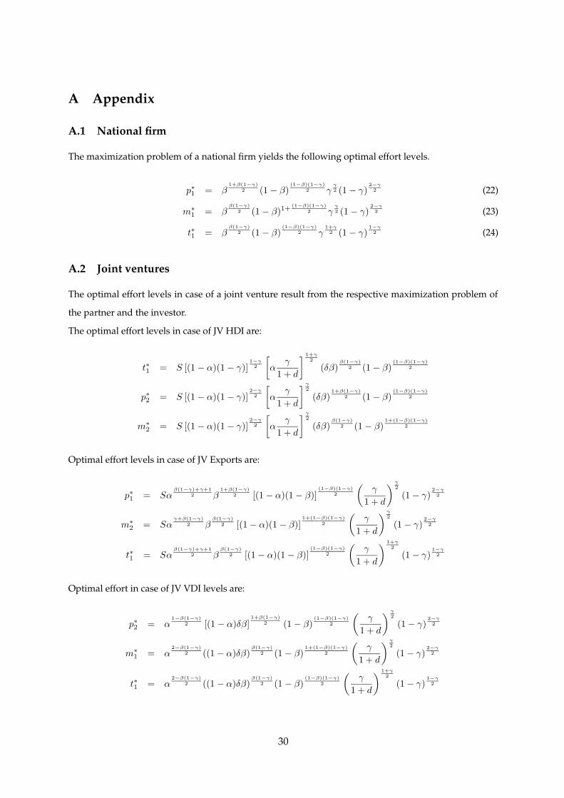
The maximization problem of a national firm yields the following optimal effort levels.
p∗1 = β1+β(1−γ)
2 (1 − β)(1−β)(1−γ)
2 γγ2 (1 − γ)
2−γ2 (22)
m∗
1 = ββ(1−γ)
2 (1 − β)1+(1−β)(1−γ)
2 γγ2 (1 − γ)
2−γ2 (23)
t∗1 = ββ(1−γ)
2 (1 − β)(1−β)(1−γ)
2 γ1+γ2 (1 − γ)
1−γ2 (24)
A.2 Joint ventures
The optimal effort levels in case of a joint venture result from the respective maximization problem of
the partner and the investor.
The optimal effort levels in case of JV HDI are:
t∗1 = S [(1 − α)(1 − γ)]1−γ
2
[
αγ
1 + d
] 1+γ2
(δβ)β(1−γ)
2 (1 − β)(1−β)(1−γ)
2
p∗2 = S [(1 − α)(1 − γ)]2−γ
2
[
αγ
1 + d
] γ2
(δβ)1+β(1−γ)
2 (1 − β)(1−β)(1−γ)
2
m∗
2 = S [(1 − α)(1 − γ)]2−γ
2
[
αγ
1 + d
] γ2
(δβ)β(1−γ)
2 (1 − β)1+(1−β)(1−γ)
2
Optimal effort levels in case of JV Exports are:
p∗1 = Sαβ(1−γ)+γ+1
2 β1+β(1−γ)
2 [(1 − α)(1 − β)](1−β)(1−γ)
2
(γ
1 + d
) γ2
(1 − γ)2−γ
2
m∗
2 = Sαγ+β(1−γ)
2 ββ(1−γ)
2 [(1 − α)(1 − β)]1+(1−β)(1−γ)
2
(γ
1 + d
) γ2
(1 − γ)2−γ
2
t∗1 = Sαβ(1−γ)+γ+1
2 ββ(1−γ)
2 [(1 − α)(1 − β)](1−β)(1−γ)
2
(γ
1 + d
) 1+γ2
(1 − γ)1−γ
2
Optimal effort in case of JV VDI levels are:
p∗2 = α1−β(1−γ)
2 [(1 − α)δβ]1+β(1−γ)
2 (1 − β)(1−β)(1−γ)
2
(γ
1 + d
) γ2
(1 − γ)2−γ
2
m∗
1 = α2−β(1−γ)
2 ((1 − α)δβ)β(1−γ)
2 (1 − β)1+(1−β)(1−γ)
2
(γ
1 + d
) γ2
(1 − γ)2−γ
2
t∗1 = α2−β(1−γ)
2 ((1 − α)δβ)β(1−γ)
2 (1 − β)(1−β)(1−γ)
2
(γ
1 + d
) 1+γ2
(1 − γ)1−γ
2
30
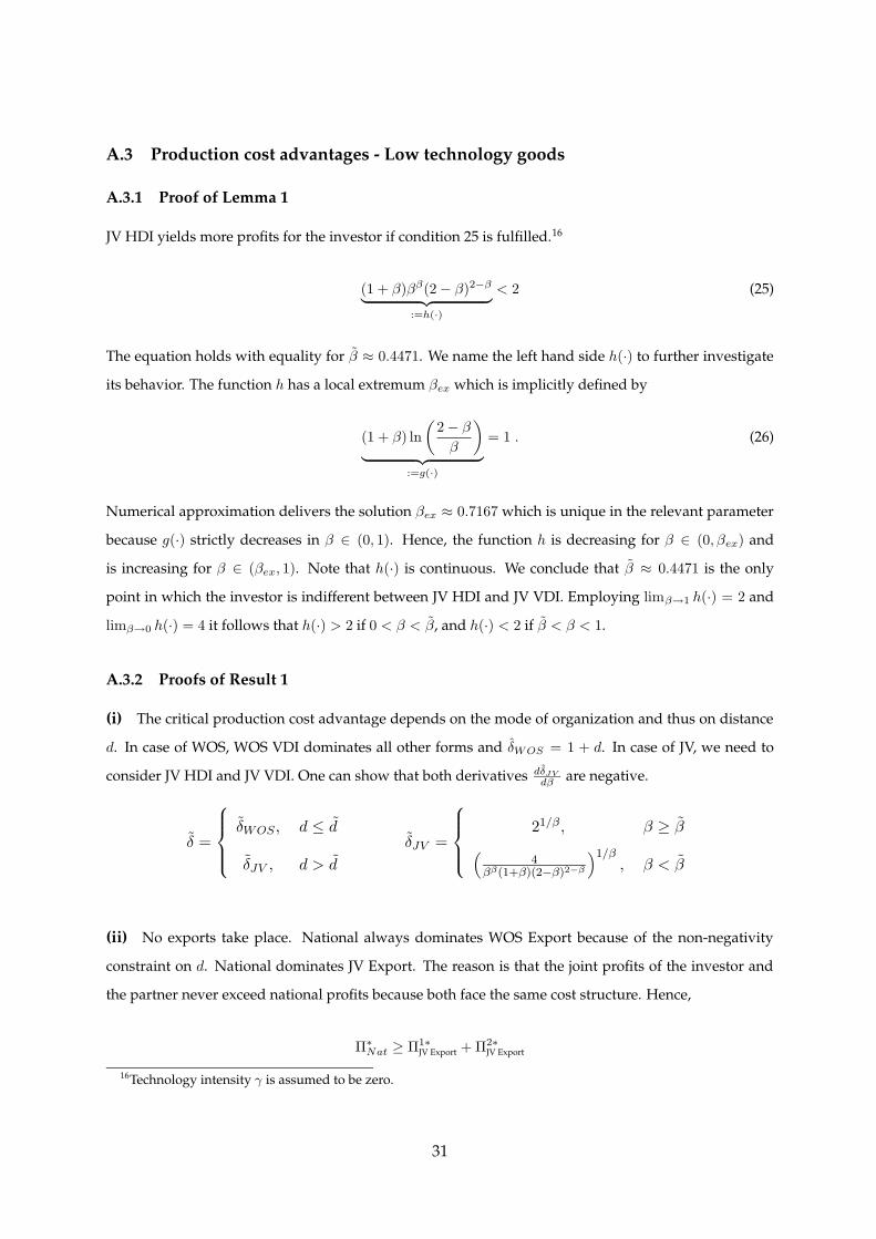
A.3 Production cost advantages - Low technology goods
A.3.1 Proof of Lemma 1
JV HDI yields more profits for the investor if condition 25 is fulfilled.16
(1 + β)ββ(2 − β)2−β
︸ ︷︷ ︸
:=h(·)
< 2 (25)
The equation holds with equality for β ≈ 0.4471. We name the left hand side h(·) to further investigate
its behavior. The function h has a local extremum βex which is implicitly defined by
(1 + β) ln
(2 − β
β
)
︸ ︷︷ ︸
:=g(·)
= 1 . (26)
Numerical approximation delivers the solution βex ≈ 0.7167 which is unique in the relevant parameter
because g(·) strictly decreases in β ∈ (0, 1). Hence, the function h is decreasing for β ∈ (0, βex) and
is increasing for β ∈ (βex, 1). Note that h(·) is continuous. We conclude that β ≈ 0.4471 is the only
point in which the investor is indifferent between JV HDI and JV VDI. Employing limβ→1 h(·) = 2 and
limβ→0 h(·) = 4 it follows that h(·) > 2 if 0 < β < β, and h(·) < 2 if β < β < 1.
A.3.2 Proofs of Result 1
(i) The critical production cost advantage depends on the mode of organization and thus on distance
d. In case of WOS, WOS VDI dominates all other forms and δWOS = 1 + d. In case of JV, we need to
consider JV HDI and JV VDI. One can show that both derivatives dδJV
dβ are negative.
δ =
δWOS , d ≤ d
δJV , d > d
δJV =
21/β , β ≥ β
(4
ββ(1+β)(2−β)2−β
)1/β, β < β
(ii) No exports take place. National always dominates WOS Export because of the non-negativity
constraint on d. National dominates JV Export. The reason is that the joint profits of the investor and
the partner never exceed national profits because both face the same cost structure. Hence,
Π∗
Nat ≥ Π1∗JV Export + Π2∗
JV Export
16Technology intensity γ is assumed to be zero.
31
As α < 1 is needed to generate joint venture revenues it follows that National leads to higher profits for
the investor.
(iii) Conditional on foreign activities we can calculate the critical distance d above which joint ventures
dominate WOS VDI. We find that d = δ − 1 and it follows directly that d decreases in β.
(iv) The result is a reformulation of Lemma 1.
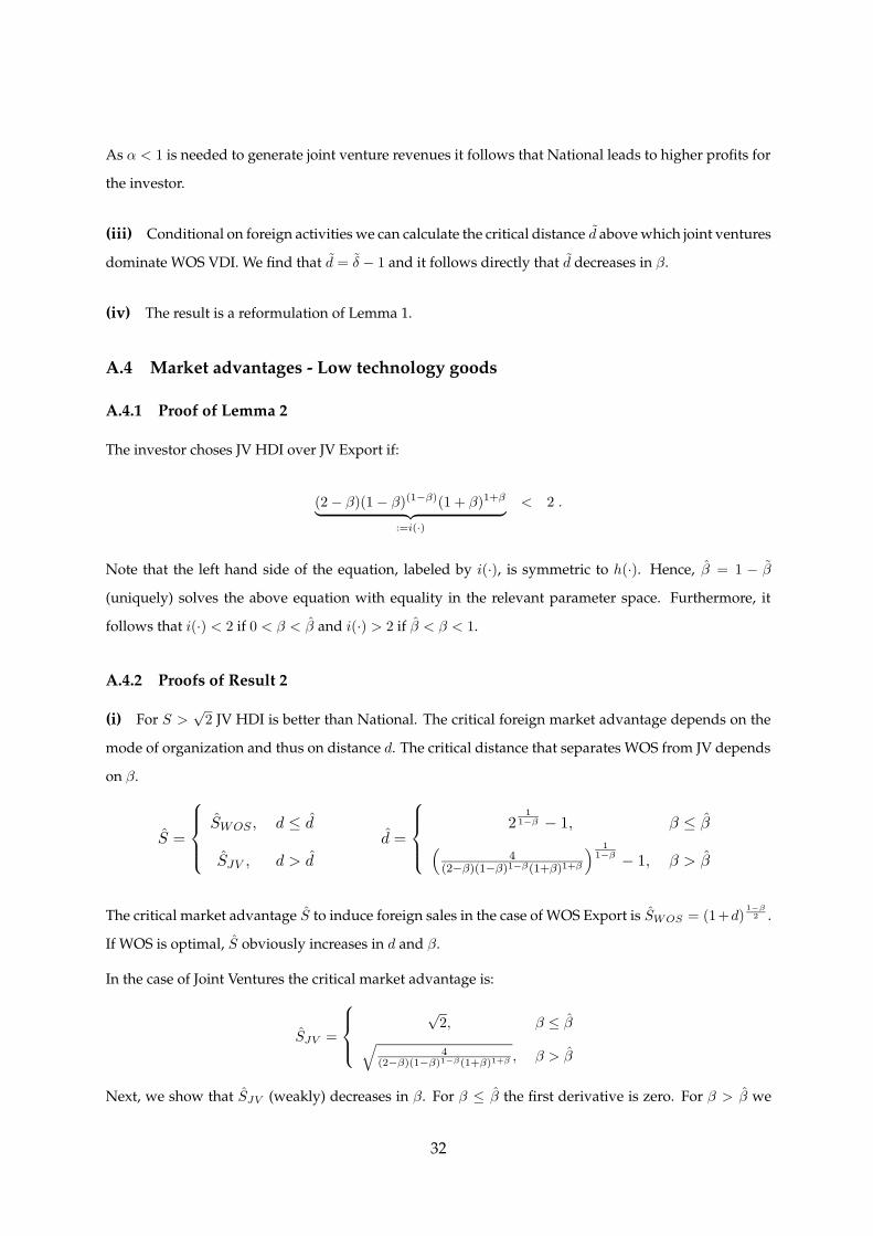
A.4 Market advantages - Low technology goods
A.4.1 Proof of Lemma 2
The investor choses JV HDI over JV Export if:
(2 − β)(1 − β)(1−β)(1 + β)1+β
︸ ︷︷ ︸
:=i(·)
< 2 .
Note that the left hand side of the equation, labeled by i(·), is symmetric to h(·). Hence, β = 1 − β
(uniquely) solves the above equation with equality in the relevant parameter space. Furthermore, it
follows that i(·) < 2 if 0 < β < β and i(·) > 2 if β < β < 1.
A.4.2 Proofs of Result 2
(i) For S >√
2 JV HDI is better than National. The critical foreign market advantage depends on the
mode of organization and thus on distance d. The critical distance that separates WOS from JV depends
on β.
S =
SWOS , d ≤ d
SJV , d > d
d =
21
1−β − 1, β ≤ β
(4
(2−β)(1−β)1−β(1+β)1+β
) 1
1−β − 1, β > β
The critical market advantage S to induce foreign sales in the case of WOS Export is SWOS = (1+d)1−β
2 .
If WOS is optimal, S obviously increases in d and β.
In the case of Joint Ventures the critical market advantage is:
SJV =
√2, β ≤ β
√4
(2−β)(1−β)1−β(1+β)1+β , β > β
Next, we show that SJV (weakly) decreases in β. For β ≤ β the first derivative is zero. For β > β we
32
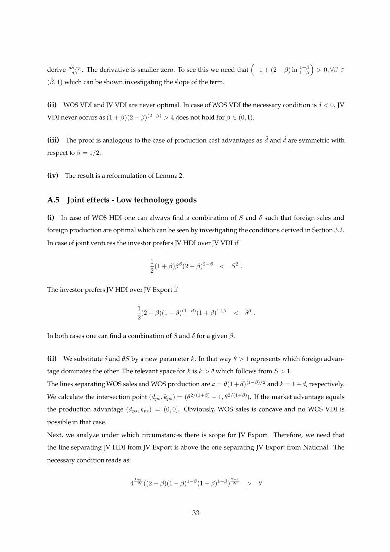
derive dSJV
dβ . The derivative is smaller zero. To see this we need that(
−1 + (2 − β) ln 1+β1−β
)
> 0,∀β ∈
(β, 1) which can be shown investigating the slope of the term.
(ii) WOS VDI and JV VDI are never optimal. In case of WOS VDI the necessary condition is d < 0. JV
VDI never occurs as (1 + β)(2 − β)(2−β) > 4 does not hold for β ∈ (0, 1).
(iii) The proof is analogous to the case of production cost advantages as d and d are symmetric with
respect to β = 1/2.
(iv) The result is a reformulation of Lemma 2.
A.5 Joint effects - Low technology goods
(i) In case of WOS HDI one can always find a combination of S and δ such that foreign sales and
foreign production are optimal which can be seen by investigating the conditions derived in Section 3.2.
In case of joint ventures the investor prefers JV HDI over JV VDI if
1
2(1 + β)ββ(2 − β)2−β < S2 .
The investor prefers JV HDI over JV Export if
1
2(2 − β)(1 − β)(1−β)(1 + β)1+β < δβ .
In both cases one can find a combination of S and δ for a given β.
(ii) We substitute δ and θS by a new parameter k. In that way θ > 1 represents which foreign advan-
tage dominates the other. The relevant space for k is k > θ which follows from S > 1.
The lines separating WOS sales and WOS production are k = θ(1+d)(1−β)/2 and k = 1+d, respectively.
We calculate the intersection point (dps, kps) = (θ2/(1+β) − 1, θ2/(1+β)). If the market advantage equals
the production advantage (dps, kps) = (0, 0). Obviously, WOS sales is concave and no WOS VDI is
possible in that case.
Next, we analyze under which circumstances there is scope for JV Export. Therefore, we need that
the line separating JV HDI from JV Export is above the one separating JV Export from National. The
necessary condition reads as:
41+β−2β ((2 − β)(1 − β)1−β(1 + β)1+β)
2+β2β > θ
33
It follows that JV Export is not implemented if θ ≥ 2. It always exist d such that JV dominates WOS. As
the left hand side is smaller than 1 for β < 0.7758, JV Export are only chosen for high β.
(iii) In order to observe JV VDI, there must be a region in which JV VDI dominates National and JV
HDI. This condition implies
(24+β
((1 + β)ββ(2 − β)(2−β))2+β
) 12β
< θ
From the above equation we see that θ has to be large to make JV VDI a viable option. It follows that no
JV VDI occurs if θ < 2. The first derivative of the left hand side with respect to β is negative if
2
βln(
(1 + β)ββ(2 − β)2−β
4) + (2 + β)
(−1
1 + βln(
2 − β
β)
)
< 0
Note, that (1 + β)ββ(2 − β)2−β equals h(·) as labeled in A.3.1. We know that h(·) < 4. It follows that
ln(%14 ) is negative. It is easy to see that
2
βln(
%1
4)
︸ ︷︷ ︸
<0
+(2 + β)
(−1
1 + βln(
2 − β
β)
)
︸ ︷︷ ︸
<0
< 0
Hence, the likelihood of JV VDI decreases in β.
A.6 Impact of technology
(i) First, we look at production cost advantages and set S = 1. We restrict ourselves to β(1−γ)−γ > 0
as no Joint Venture would occur otherwise. It follows that γ < β1+β , and for β ∈ (0, 1) that γ < 1/2. JV
HDI dominates WOS VDI if distance d is greater than d which is defined by
(1 + d)β(1−γ)−γ =4
(1 − γ)1−γ(1 + γ)1+γ(2 − γ).
The first derivative of the critical distance ∂d/∂γ is positive if
(1 + β) ln( 4%1 )
(β(1 − γ) − γ)+ ln(1 − γ) − ln(1 + γ) +
1
2 − γ> 0 ,
where %1 = (1 − γ)1−γ(1 + γ)1+γ(2 − γ). We can show that the above equation holds for γ < 1/2 by
investigating minimum values of the left hand side.
In case of JV VDI d also increases in γ. JV VDI dominates WOS VDI if distance d is greater than d which
34

is given by
(d + 1)ρ−γ =4
(2 − ρ)(2−ρ)(1 + ρ)ρρ
where ρ := β(1 − γ). We have already shown that
(4
(2 − ρ)(2−ρ)(1 + ρ)ρρ
) 1ρ
decreases in ρ. Furthermore, it is true that(
4(2−ρ)(2−ρ)(1+ρ)ρρ
)
> 1. As we increase γ we decrease ρ. This
leads to an increase of the critical distance d.
The proofs in case of market advantages (δ = 1) are analogous to the once above if we replace the weight
on production β(1 − γ) by the weight on marketing (1 − β)(1 − γ).
(ii) We show that joint ventures become less attractive as compared to National if γ increases. In (iii)
we show that JV is never optimal for for γ > 1/2.
JV HDI dominates National if
S2δβ(1−γ) >4(1 + d)γ
(1 − γ)1−γ(1 + γ)1+γ(2 − γ)︸ ︷︷ ︸
:=s(·)
.
JV HDI is not profitable if d ≤ 1 as WOS HDI dominates JV HDI in that case. The left hand side (weakly)
decreases in γ, making JV HDI less likely. The right hand side of the above equation increases in γ, also
making JV HDI less likely. The necessary condition is
∂s(·)∂γ
> 0
⇒ ln
(1 − γ
1 + γ
)
+1
2 − γ+ ln(1 + d) > 0
The equation holds for d ≥ 1 and γ < 0.53. Hence, JV HDI becomes less likely as the importance of
technology γ increases in the relevant cases.
JV Export dominates National if
S2 >4(1 + d)γ
ρρ(2 − ρ)(2−ρ)(1 + ρ)︸ ︷︷ ︸
:=v(·)
,
where ρ = (1−β)(1−γ). The right hand side, named v(·), increases in γ, i.e. a higher foreign advantage
35
is needed in order to make JV Export better than National. The crucial condition is
(1 − β) ln(ρ) − (1 − β) ln(2 − ρ) +1 − β
1 + ρ+ ln(1 + d) > 0
Exploiting the two limitations d > 1 and ρ > γ, it can be shown that the above equation holds.
The proof for JV VDI is analogous to JV Export replacing ρ := (1 − β)(1 − γ) with ρ2 := β(1 − γ) which
reflects the weight on the production activity.
(iii) Joint ventures are never optimal if γ > 0.5 because for each JV there exists at least one WOS that
pays strictly higher profits to the investor. Each joint venture is dominated by its respective WOS.
JV Export dominates WOS Export if
(1 + d)(1−β)(1−γ)−γ(1 + (1 − β)(1 − γ))
((1 − β)(1 − γ))((1−β)(1−γ))(2 − (1 − β)(1 − γ))(2−(1−β)(1−γ)) > 4
Using maximum values on the left hand side we are left to show that
(1 + (1 − β)(1 − γ))(2 − (1 − β)(1 − γ))2 > 4
never holds. The solutions to the polynomial w.r.t. γ, 1 and β+2β+1 , are both out of (0, 1). By plugging
numbers it follows that WOS Export is better than JV Export for γ ∈ ( 12 , 1).
The proofs for VDI and HDI are analogously.
(iv) The first derivatives of the investor’s optimal ownership shares with respect to technology inten-
sity γdα∗
JV Export
dγ = 1/2(1 − β),dα∗
JV VDI
dγ = 1/2β, andα∗
JV HDI
dγ = 1/2 are all greater than zero.
36