Embed Size (px)
Citation preview
Huang et al:MTG-IRS OSSE. EMC seminar, 1/11/2008. 1
MTG-IRS: An Observing System SimulationExperiment (OSSE) on regional scales
Xiang-Yu Huang, Hongli Wang, Yongsheng ChenNational Center for Atmospheric Research, Boulder, Colorado, U.S.A.
Xin ZhangUniversity of Hawaii, Honolulu. Hawaii, U.S.A.
Stephen A. Tjemkes, Rolf StuhlmannEUMETSAT, Darmstadt, Germany
Huang et al:MTG-IRS OSSE. EMC seminar, 1/11/2008. 2
Contents
• Background• The nature run (MM5)• Calibration experiments (WRF)• MTG-IRS retrievals• Data assimilation and forecast results (WRF)• Summary• Future work• Identical twin experiments
Huang et al:MTG-IRS OSSE. EMC seminar, 1/11/2008. 3
Background• IRS sounding Mission on MTG will provide high-resolution data
which includes temperature and water vapor information.• Realistic mesoscale details in moisture are important for
forecasting convective events (e.g., Koch et al. 1997; Parsons etal. 2000; Weckwerth 2000, 2004).
• Objective: To document the added value of water vaporobservations derived from a hyperspectral infrared soundinginstrument on a geostationary satellite for regionalforecasting.
Huang et al:MTG-IRS OSSE. EMC seminar, 1/11/2008. 4
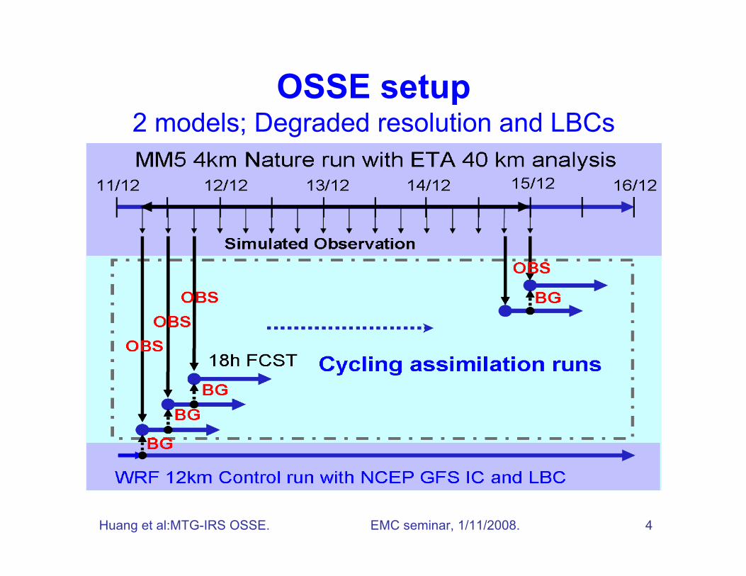
OSSE setup2 models; Degraded resolution and LBCs
Huang et al:MTG-IRS OSSE. EMC seminar, 1/11/2008. 5
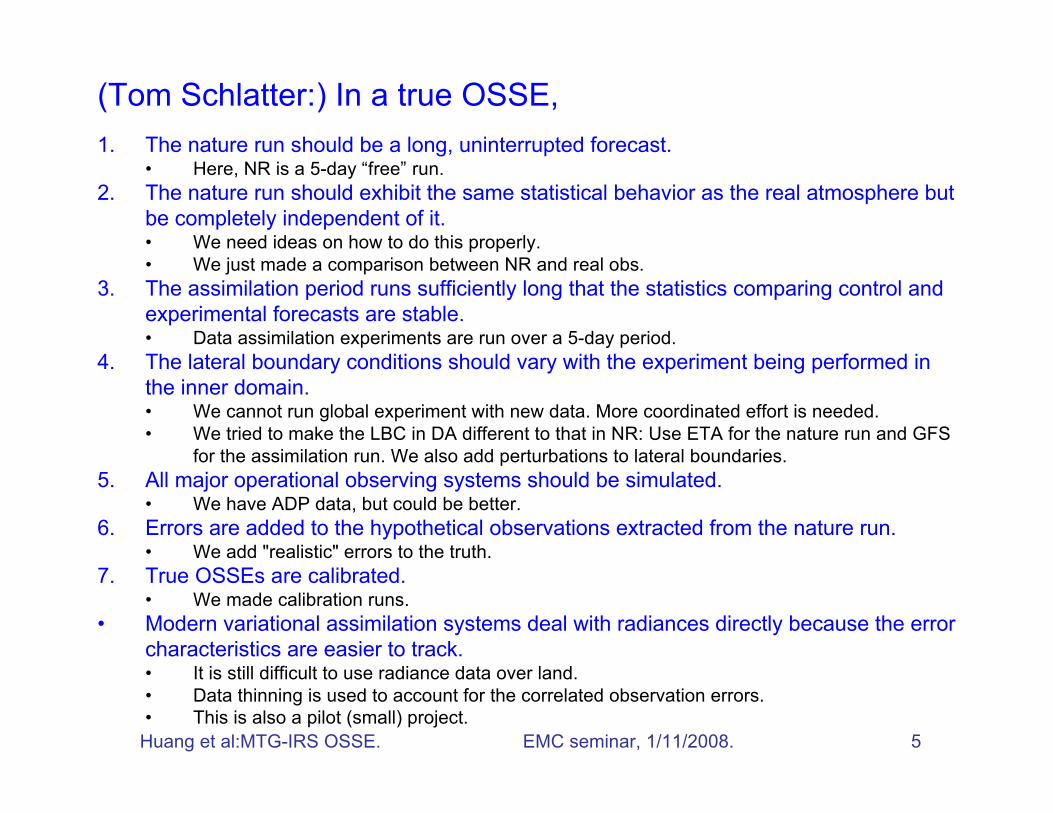
1. The nature run should be a long, uninterrupted forecast.• Here, NR is a 5-day “free” run.
2. The nature run should exhibit the same statistical behavior as the real atmosphere butbe completely independent of it.• We need ideas on how to do this properly.• We just made a comparison between NR and real obs.
3. The assimilation period runs sufficiently long that the statistics comparing control andexperimental forecasts are stable.• Data assimilation experiments are run over a 5-day period.
4. The lateral boundary conditions should vary with the experiment being performed inthe inner domain.• We cannot run global experiment with new data. More coordinated effort is needed.• We tried to make the LBC in DA different to that in NR: Use ETA for the nature run and GFS
for the assimilation run. We also add perturbations to lateral boundaries.5. All major operational observing systems should be simulated.
• We have ADP data, but could be better.6. Errors are added to the hypothetical observations extracted from the nature run.
• We add "realistic" errors to the truth.7. True OSSEs are calibrated.
• We made calibration runs.• Modern variational assimilation systems deal with radiances directly because the error
characteristics are easier to track.• It is still difficult to use radiance data over land.• Data thinning is used to account for the correlated observation errors.• This is also a pilot (small) project.
(Tom Schlatter:) In a true OSSE,
Huang et al:MTG-IRS OSSE. EMC seminar, 1/11/2008. 6
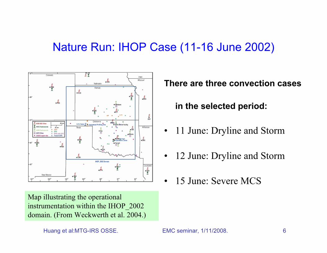
Nature Run: IHOP Case (11-16 June 2002)
There are three convection cases
in the selected period:
• 11 June: Dryline and Storm
• 12 June: Dryline and Storm
• 15 June: Severe MCSMap illustrating the operationalinstrumentation within the IHOP_2002domain. (From Weckwerth et al. 2004.)
Huang et al:MTG-IRS OSSE. EMC seminar, 1/11/2008. 7
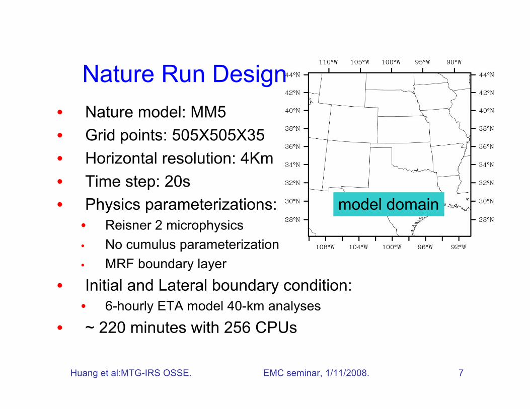
Nature Run Design• Nature model: MM5• Grid points: 505X505X35• Horizontal resolution: 4Km• Time step: 20s• Physics parameterizations:
• Reisner 2 microphysics• No cumulus parameterization• MRF boundary layer
• Initial and Lateral boundary condition:• 6-hourly ETA model 40-km analyses
• ~ 220 minutes with 256 CPUs
model domain
Huang et al:MTG-IRS OSSE. EMC seminar, 1/11/2008. 8
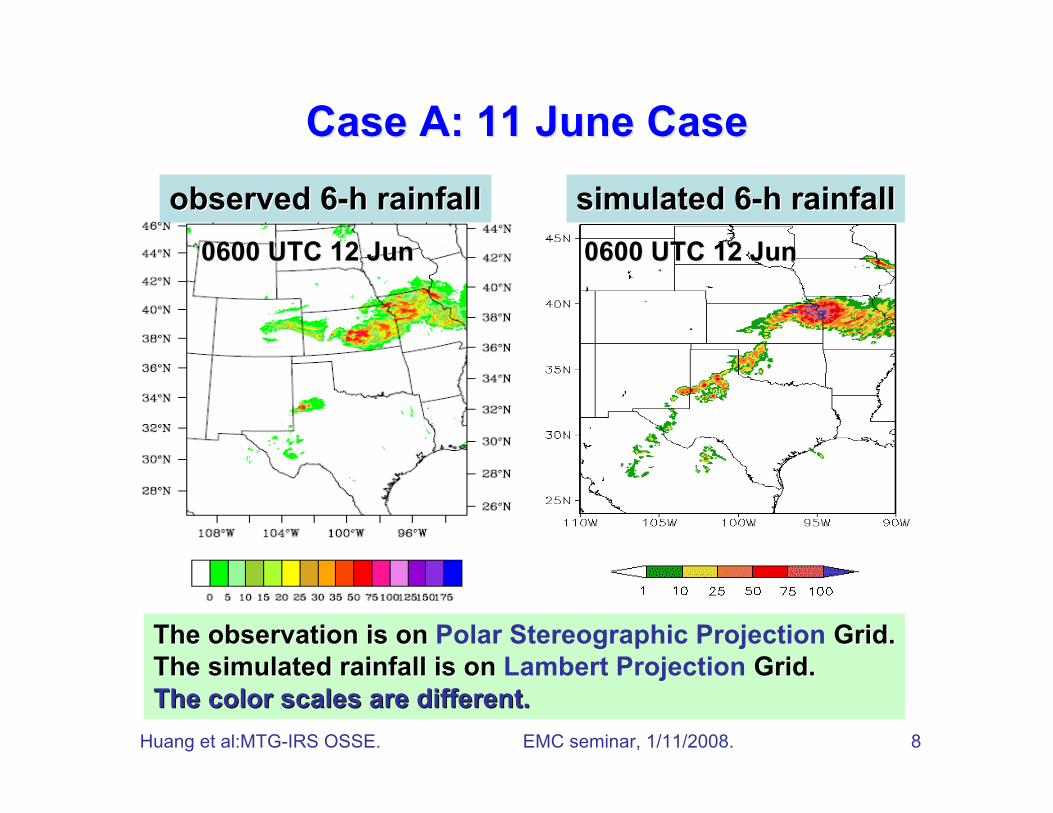
observed 6-h rainfallobserved 6-h rainfall simulated 6-h rainfallsimulated 6-h rainfall
The observation is on The observation is on Polar Stereographic Projection Grid. Grid.The simulated rainfall is on The simulated rainfall is on Lambert Projection Grid. Grid.The color scales are different.The color scales are different.
0600 UTC 12 Jun0600 UTC 12 Jun 0600 UTC 12 Jun0600 UTC 12 Jun
Case A: 11 June CaseCase A: 11 June Case
Huang et al:MTG-IRS OSSE. EMC seminar, 1/11/2008. 9
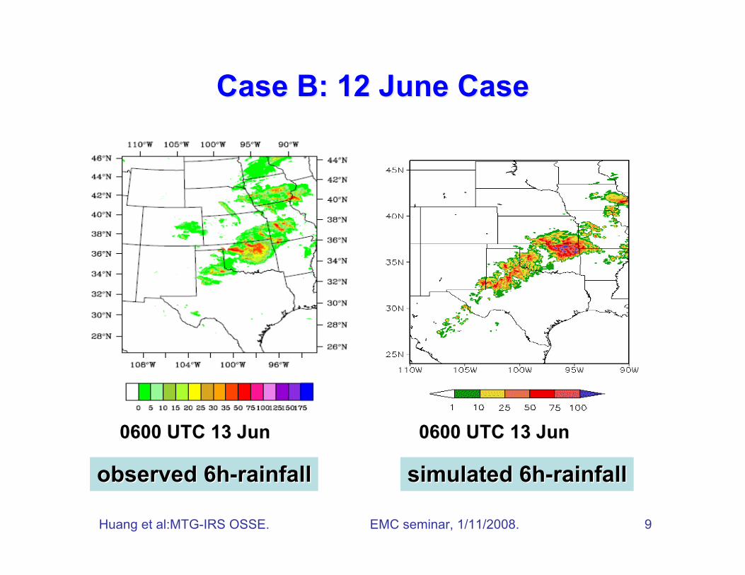
observed 6h-rainfallobserved 6h-rainfall simulated 6h-rainfallsimulated 6h-rainfall
0600 UTC 13 Jun0600 UTC 13 Jun 0600 UTC 13 Jun0600 UTC 13 Jun
Case B: 12 June CaseCase B: 12 June Case
Huang et al:MTG-IRS OSSE. EMC seminar, 1/11/2008. 10
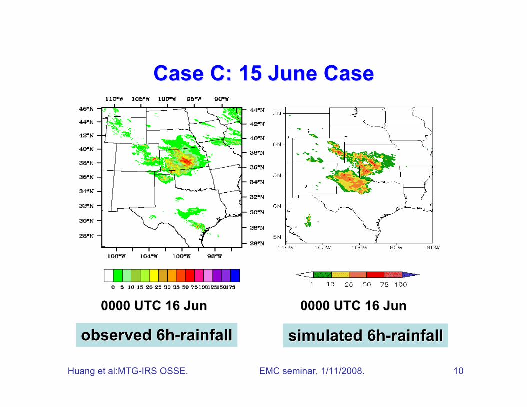
Case C: 15 June CaseCase C: 15 June Case
observed 6h-rainfallobserved 6h-rainfall simulated 6h-rainfallsimulated 6h-rainfall
0000 UTC 16 Jun0000 UTC 16 Jun 0000 UTC 16 Jun0000 UTC 16 Jun
Huang et al:MTG-IRS OSSE. EMC seminar, 1/11/2008. 11
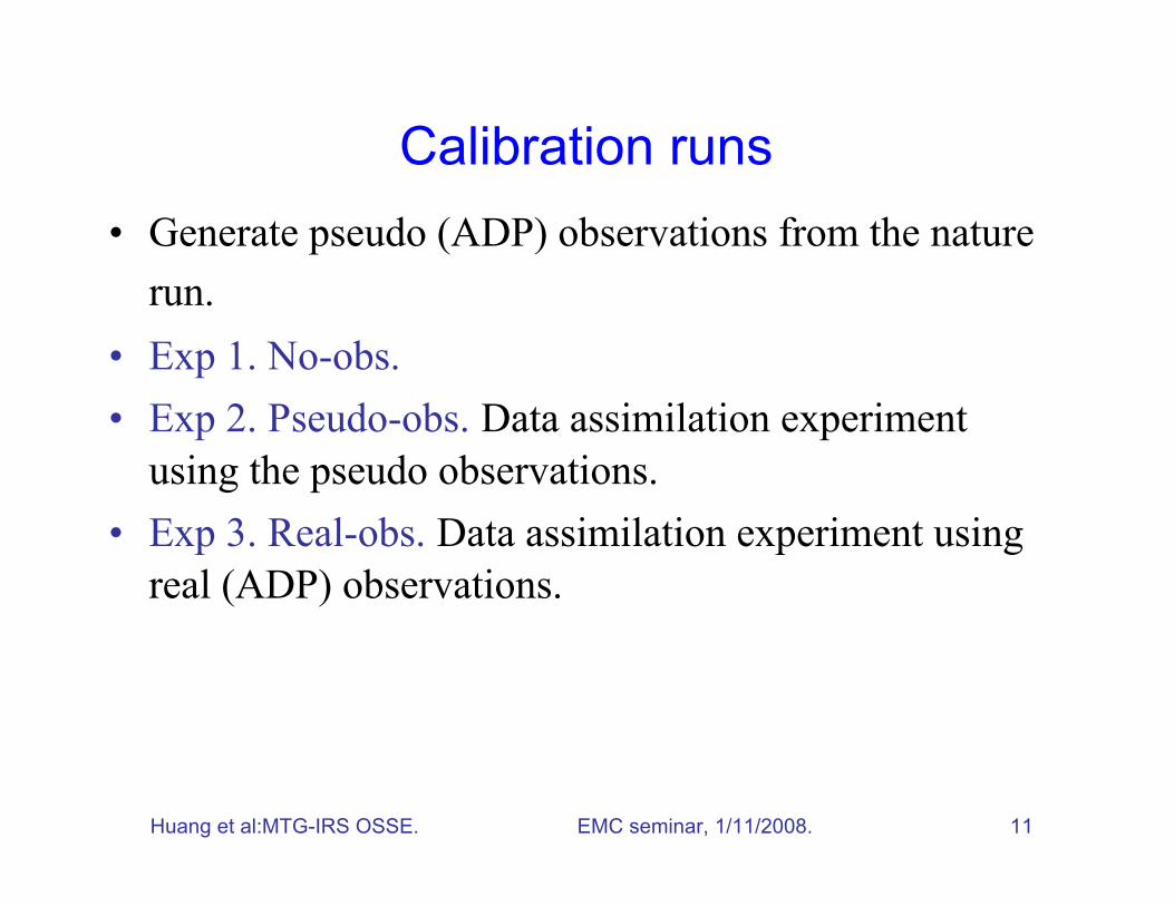
Calibration runs• Generate pseudo (ADP) observations from the nature
run.• Exp 1. No-obs.• Exp 2. Pseudo-obs. Data assimilation experiment
using the pseudo observations.• Exp 3. Real-obs. Data assimilation experiment using
real (ADP) observations.
Huang et al:MTG-IRS OSSE. EMC seminar, 1/11/2008. 12
Simulated Dataset
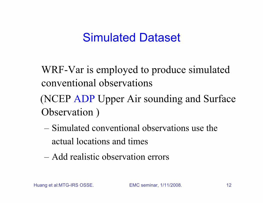
WRF-Var is employed to produce simulatedconventional observations
(NCEP ADP Upper Air sounding and SurfaceObservation )– Simulated conventional observations use the
actual locations and times
– Add realistic observation errors
Huang et al:MTG-IRS OSSE. EMC seminar, 1/11/2008. 13
Simulated Dataset
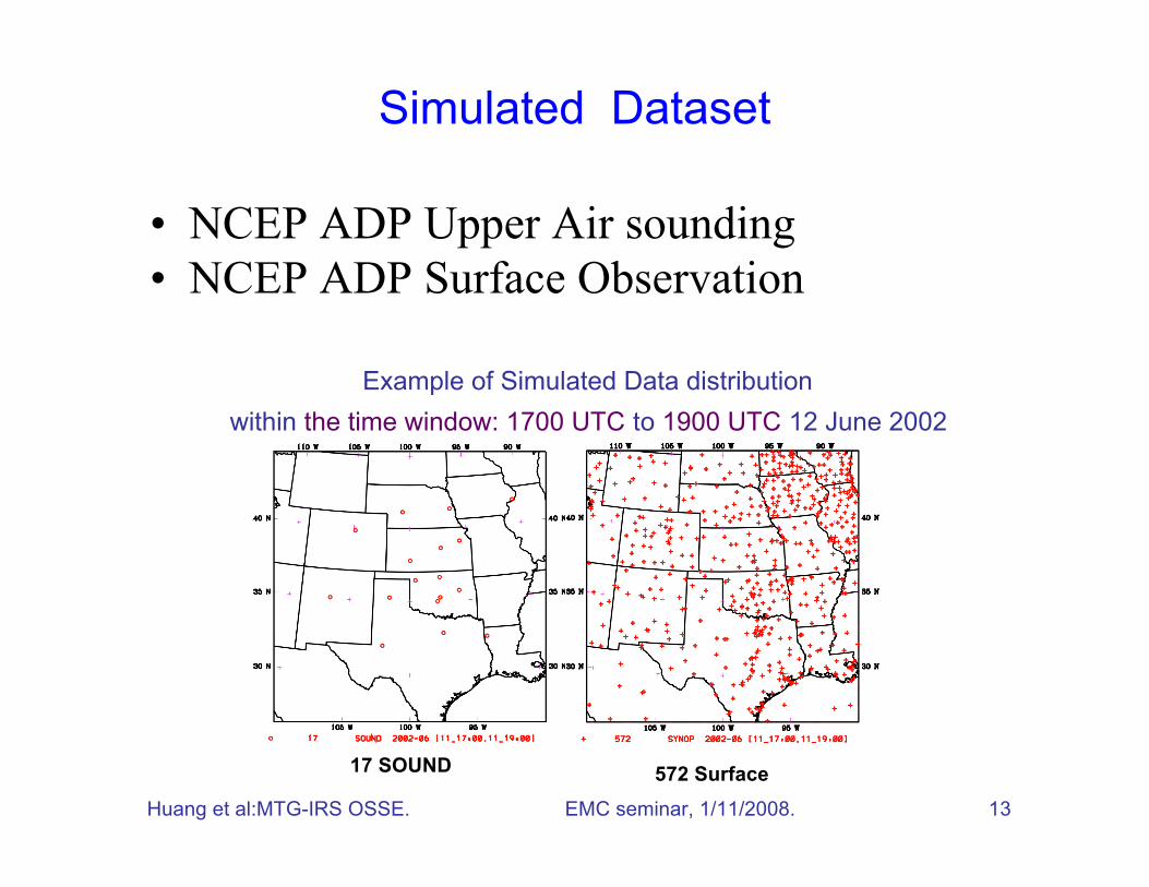
• NCEP ADP Upper Air sounding• NCEP ADP Surface Observation
572 Surface17 SOUND
Example of Simulated Data distributionwithin the time window: 1700 UTC to 1900 UTC 12 June 2002
Huang et al:MTG-IRS OSSE. EMC seminar, 1/11/2008. 14
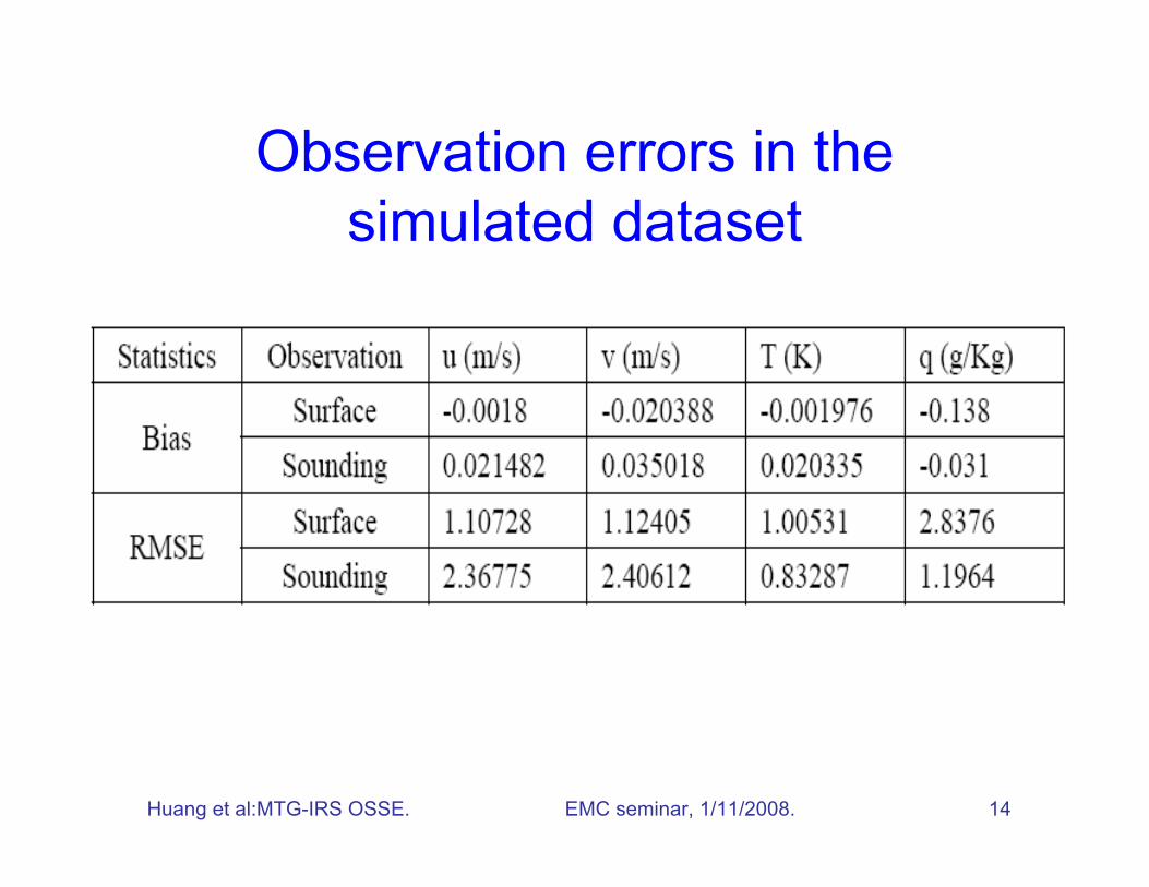
Observation errors in thesimulated dataset
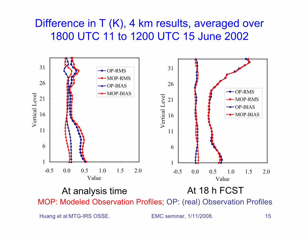
Huang et al:MTG-IRS OSSE. EMC seminar, 1/11/2008. 15
MOP: Modeled Observation Profiles; OP: (real) Observation Profiles
Difference in T (K), 4 km results, averaged over1800 UTC 11 to 1200 UTC 15 June 2002
At analysis time At 18 h FCST
1
6
11
16
21
26
31
-0.5 0.0 0.5 1.0 1.5 2.0
Value
Vert
ical
Lev
el
OP-RMS
MOP-RMS
OP-BIAS
MOP-BIAS
1
6
11
16
21
26
31
-0.5 0.0 0.5 1.0 1.5 2.0
Value
Vert
ical
Lev
el OP-RMS
MOP-RMS
OP-BIAS
MOP-BIAS
Huang et al:MTG-IRS OSSE. EMC seminar, 1/11/2008. 16
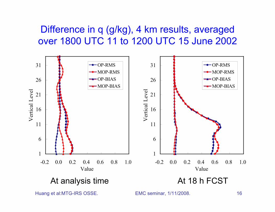
Difference in q (g/kg), 4 km results, averagedover 1800 UTC 11 to 1200 UTC 15 June 2002
At analysis time At 18 h FCST
1
6
11
16
21
26
31
-0.2 0.0 0.2 0.4 0.6 0.8 1.0
Value
Vert
ical
Lev
el
OP-RMS
MOP-RMS
OP-BIAS
MOP-BIAS
1
6
11
16
21
26
31
-0.2 0.0 0.2 0.4 0.6 0.8 1.0
Value
Vert
ical
Lev
el
OP-RMS
MOP-RMS
OP-BIAS
MOP-BIAS
Huang et al:MTG-IRS OSSE. EMC seminar, 1/11/2008. 17
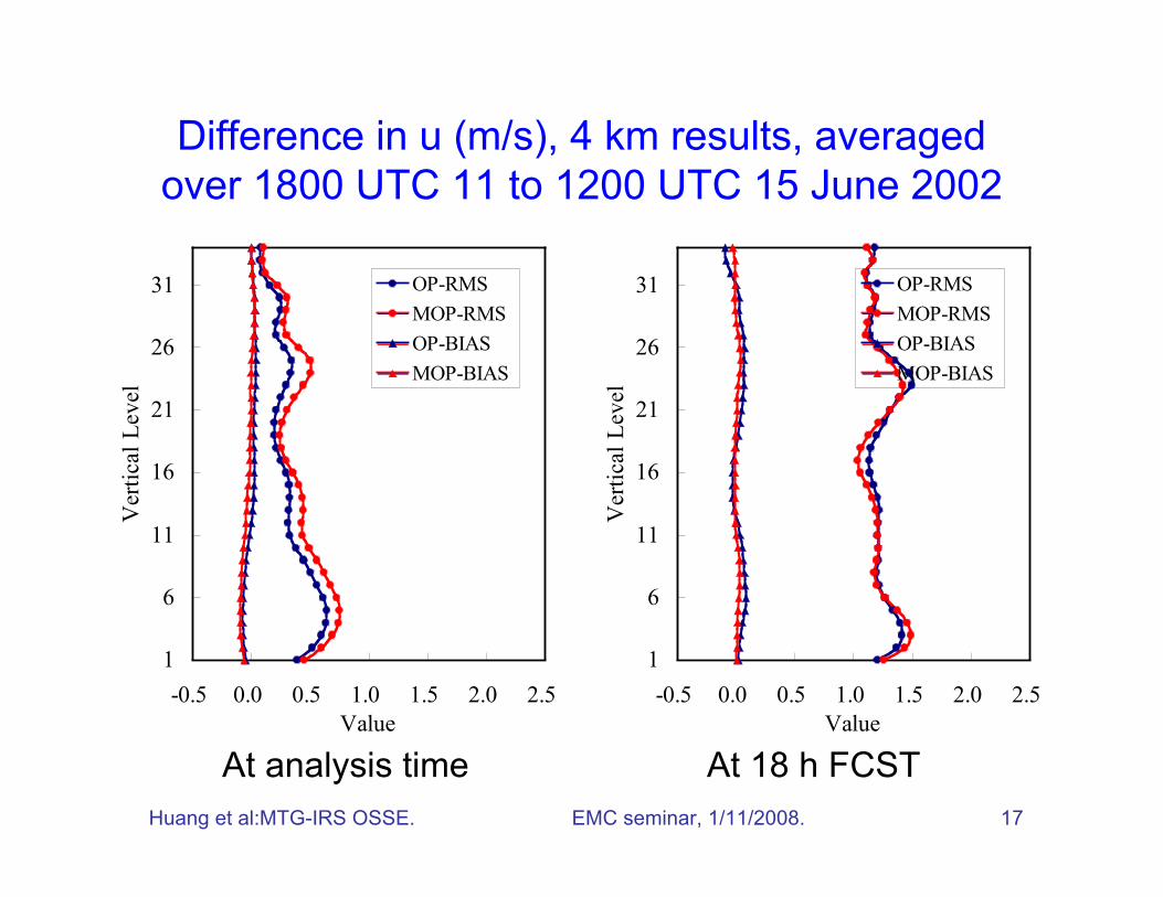
Difference in u (m/s), 4 km results, averagedover 1800 UTC 11 to 1200 UTC 15 June 2002
At analysis time At 18 h FCST
1
6
11
16
21
26
31
-0.5 0.0 0.5 1.0 1.5 2.0 2.5
Value
Vert
ical
Lev
el
OP-RMS
MOP-RMS
OP-BIAS
MOP-BIAS
1
6
11
16
21
26
31
-0.5 0.0 0.5 1.0 1.5 2.0 2.5
Value
Vert
ical
Lev
el
OP-RMS
MOP-RMS
OP-BIAS
MOP-BIAS
Huang et al:MTG-IRS OSSE. EMC seminar, 1/11/2008. 18
MTG-IRS Retrieval (I)Forward calculations
• Profile information for the forward calculations arecombination of climatology (above 50 hPa) and MM5results (below 50 hPa), Ozone information isextracted from climatology. For each hour for fivedays 505 x 505 profiles (= one “data cube”).
• RTM adopted is same code as used for HES/GIFTStrade-off studies by SSEC, which is a statisticalmodel. Only clear sky calculations, accuracy is notknown.
• CPU: To generate R(toa) for one “data cube” takesabout 20 hours CPU.
Huang et al:MTG-IRS OSSE. EMC seminar, 1/11/2008. 19
MTG-IRS Retrieval (II)Inverse Calculations
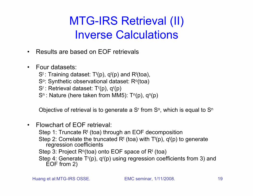
• Results are based on EOF retrievals
• Four datasets:St : Training dataset: Tt(p), qt(p) and Rt(toa),So: Synthetic observational dataset: Ro(toa)Sr : Retrieval dataset: Tr(p), qr(p)Sn : Nature (here taken from MM5): Tn(p), qn(p)
Objective of retrieval is to generate a Sr from So, which is equal to Sn
• Flowchart of EOF retrieval:Step 1: Truncate Rt (toa) through an EOF decompositionStep 2: Correlate the truncated Rt (toa) with Tt(p), qt(p) to generate
regression coefficientsStep 3: Project Ro(toa) onto EOF space of Rt (toa)Step 4: Generate Tr(p), qr(p) using regression coefficients from 3) and
EOF from 2)
Huang et al:MTG-IRS OSSE. EMC seminar, 1/11/2008. 20
Two EOF Training methodsTwo different training methods applied:
Global Training: generated a “global dataset” by randomselection of profiles from a number data cubescovering dynamical range of the diurnal cycle. About100000 profiles, a single training dataset
As this global dataset had different properties than anindividual data-cube; assimilation generated notsatisfactory results (mainly because of bias)
“Bias free Training”: For each datacube a separatetraining dataset consisting of 10% of the data in theparticular datacube.

Huang et al:MTG-IRS OSSE. EMC seminar, 1/11/2008. 21
Simulated Dataset
• NCEP ADP Upper Air sounding• NCEP ADP Surface Observation• MTG-IRS retrieved profiles
572 Surface17 SOUND 10706 MTG-IRS RP
Example of Simulated Data distributionwithin the time window: 1700 UTC to 1900 UTC 12 June 2002
Huang et al:MTG-IRS OSSE. EMC seminar, 1/11/2008. 22
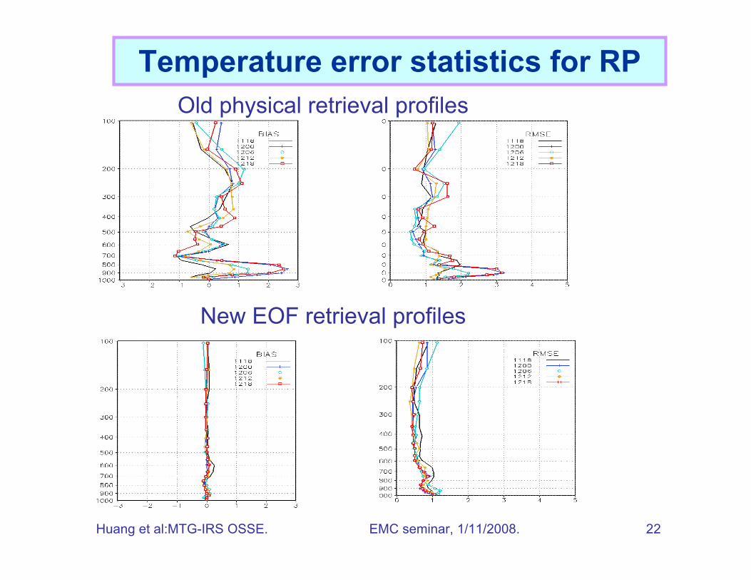
Old physical retrieval profiles
New EOF retrieval profiles
Temperature error statistics for RP
Huang et al:MTG-IRS OSSE. EMC seminar, 1/11/2008. 23
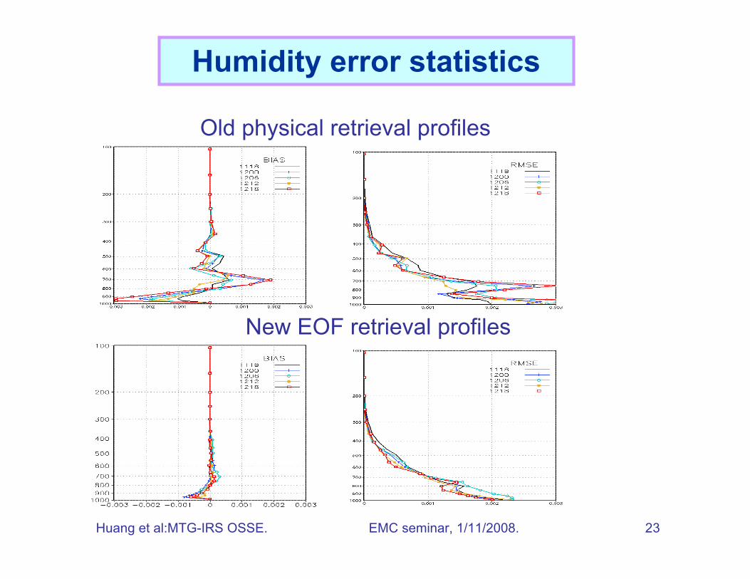
Humidity error statistics
Old physical retrieval profiles
New EOF retrieval profiles
Huang et al:MTG-IRS OSSE. EMC seminar, 1/11/2008. 24
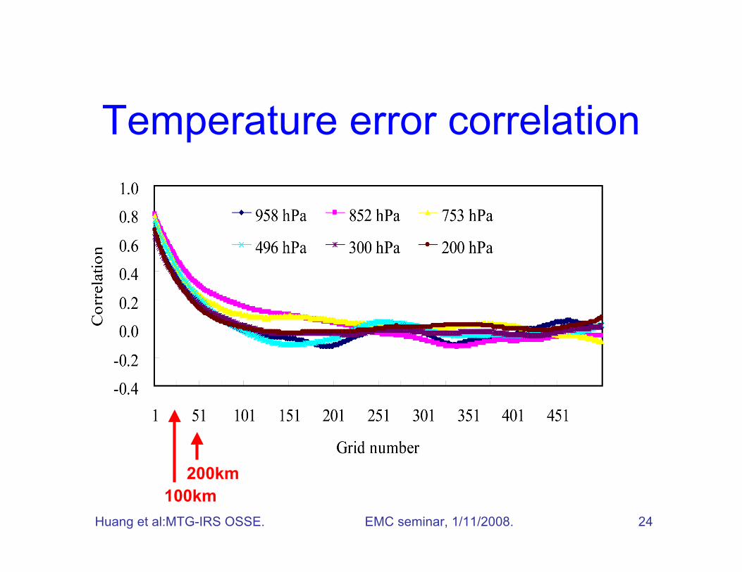
Temperature error correlation
200km100km
Huang et al:MTG-IRS OSSE. EMC seminar, 1/11/2008. 25
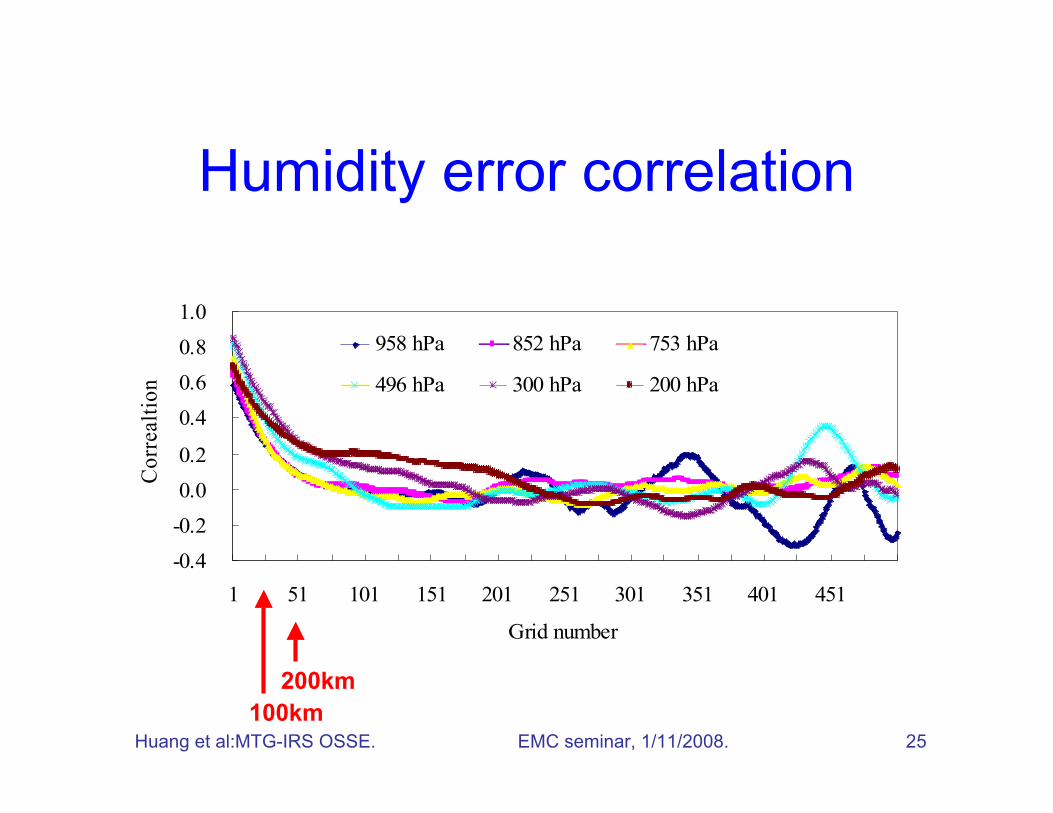
Humidity error correlation
-0.4
-0.2
0.0
0.2
0.4
0.6
0.8
1.0
1 51 101 151 201 251 301 351 401 451
Grid number
Co
rrealt
ion
958 hPa 852 hPa 753 hPa
496 hPa 300 hPa 200 hPa
200km100km
Huang et al:MTG-IRS OSSE. EMC seminar, 1/11/2008. 26
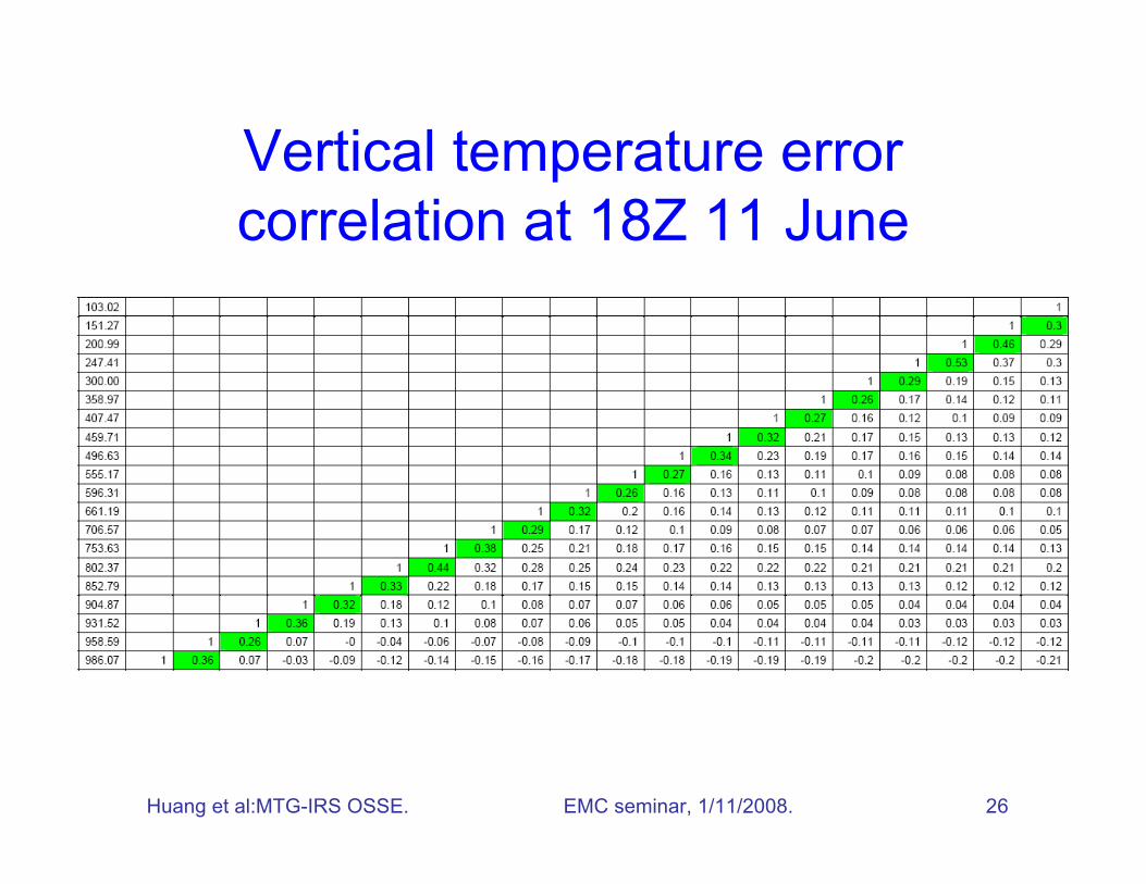
Vertical temperature errorcorrelation at 18Z 11 June
Huang et al:MTG-IRS OSSE. EMC seminar, 1/11/2008. 27
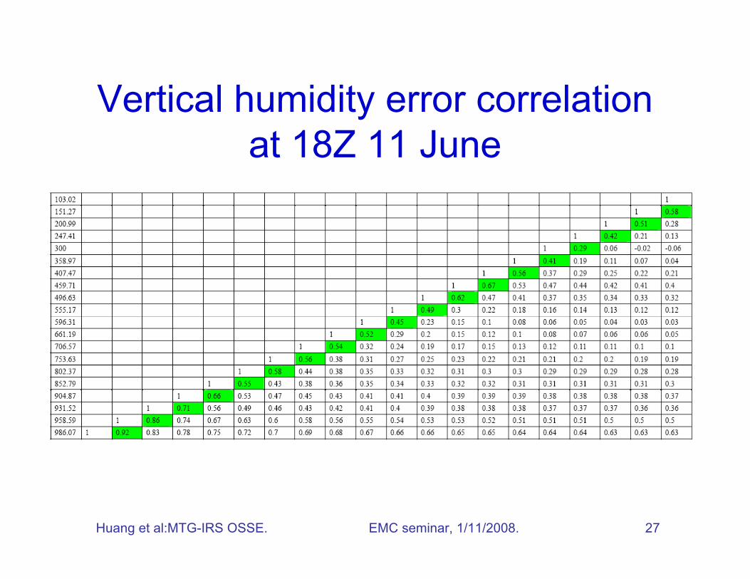
Vertical humidity error correlationat 18Z 11 June
Huang et al:MTG-IRS OSSE. EMC seminar, 1/11/2008. 28
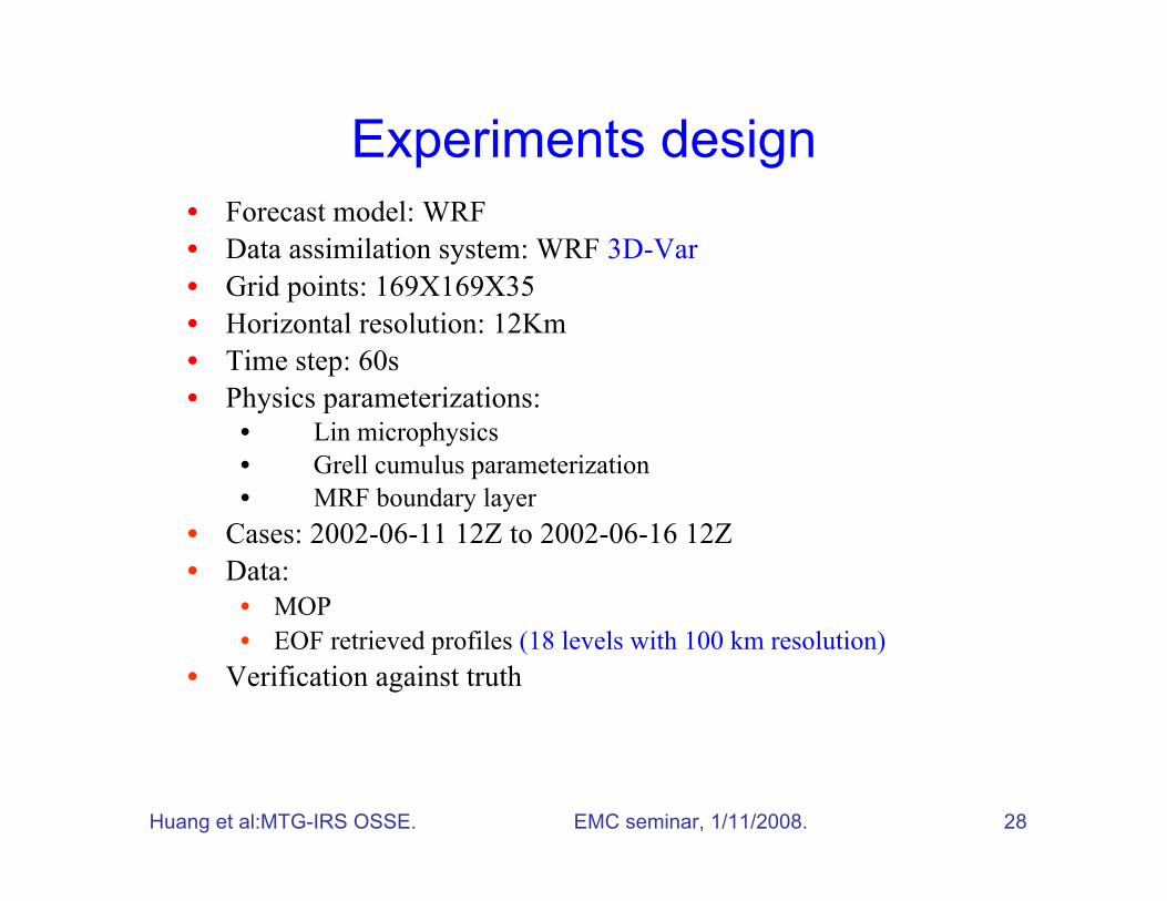
Experiments design• Forecast model: WRF• Data assimilation system: WRF 3D-Var• Grid points: 169X169X35• Horizontal resolution: 12Km• Time step: 60s• Physics parameterizations:
• Lin microphysics• Grell cumulus parameterization• MRF boundary layer
• Cases: 2002-06-11 12Z to 2002-06-16 12Z• Data:
• MOP• EOF retrieved profiles (18 levels with 100 km resolution)
• Verification against truth
Huang et al:MTG-IRS OSSE. EMC seminar, 1/11/2008. 29
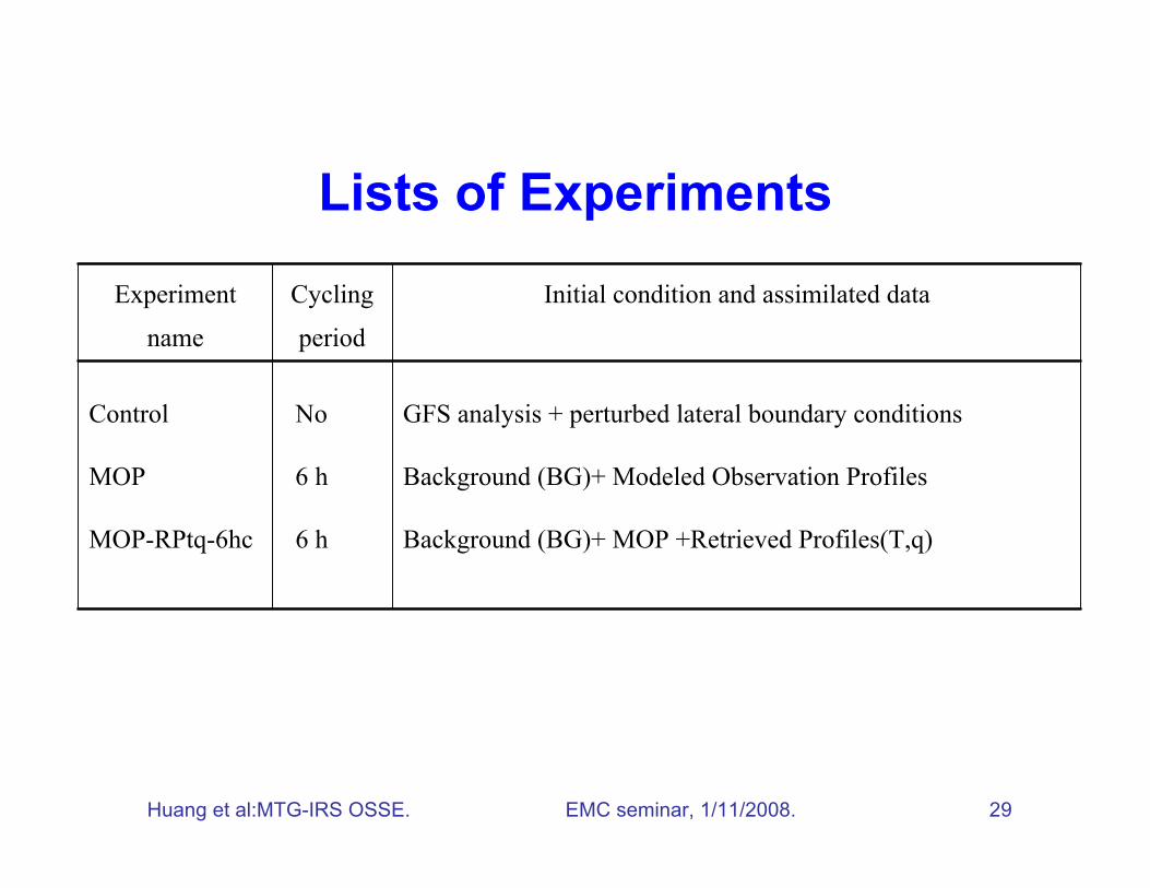
Lists of Experiments
GFS analysis + perturbed lateral boundary conditions
Background (BG)+ Modeled Observation Profiles
Background (BG)+ MOP +Retrieved Profiles(T,q)
No
6 h
6 h
Control
MOP
MOP-RPtq-6hc
Initial condition and assimilated dataCycling
period
Experiment
name
Huang et al:MTG-IRS OSSE. EMC seminar, 1/11/2008. 30
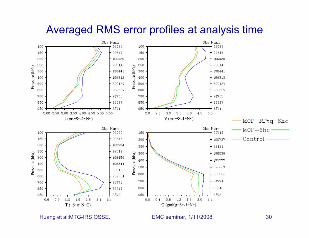
Averaged RMS error profiles at analysis time
Huang et al:MTG-IRS OSSE. EMC seminar, 1/11/2008. 31
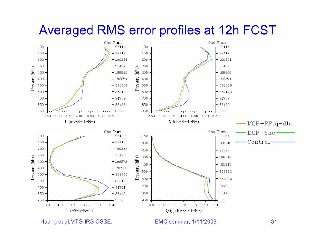
Averaged RMS error profiles at 12h FCST
Huang et al:MTG-IRS OSSE. EMC seminar, 1/11/2008. 32
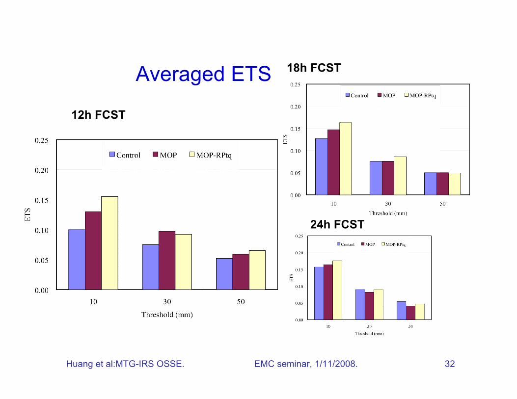
Averaged ETS
12h FCST
18h FCST
24h FCST
Huang et al:MTG-IRS OSSE. EMC seminar, 1/11/2008. 33
(64,64)
4Dvar
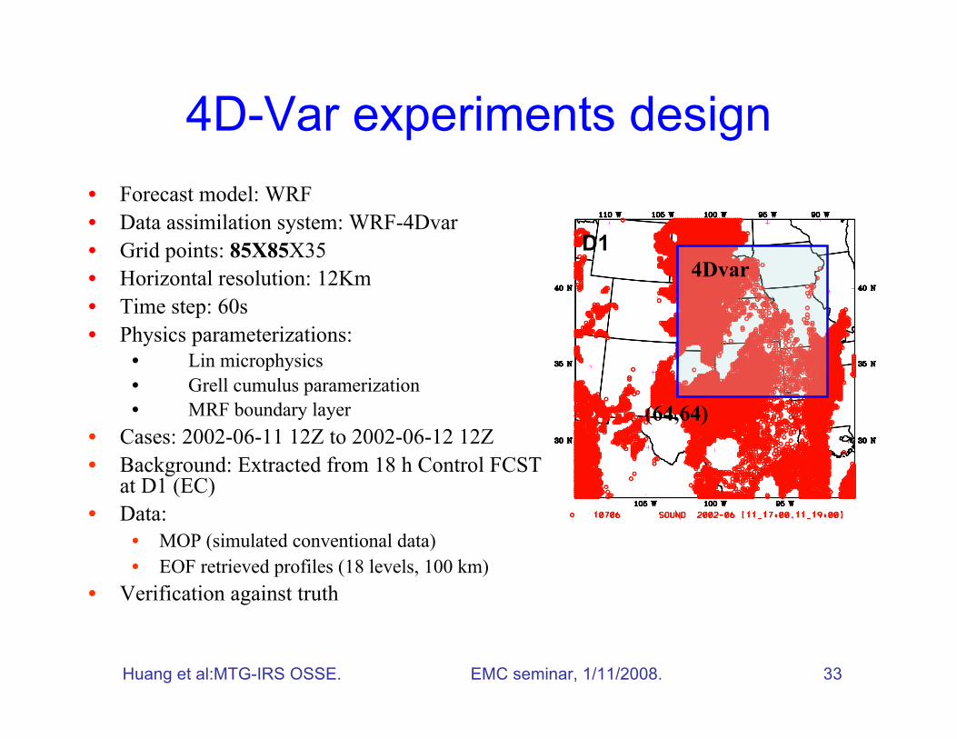
• Forecast model: WRF• Data assimilation system: WRF-4Dvar• Grid points: 85X85X35• Horizontal resolution: 12Km• Time step: 60s• Physics parameterizations:
• Lin microphysics• Grell cumulus paramerization• MRF boundary layer
• Cases: 2002-06-11 12Z to 2002-06-12 12Z• Background: Extracted from 18 h Control FCST
at D1 (EC)• Data:
• MOP (simulated conventional data)• EOF retrieved profiles (18 levels, 100 km)
• Verification against truth
4D-Var experiments design
D1
Huang et al:MTG-IRS OSSE. EMC seminar, 1/11/2008. 34
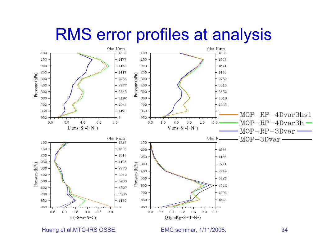
RMS error profiles at analysistime
Huang et al:MTG-IRS OSSE. EMC seminar, 1/11/2008. 35
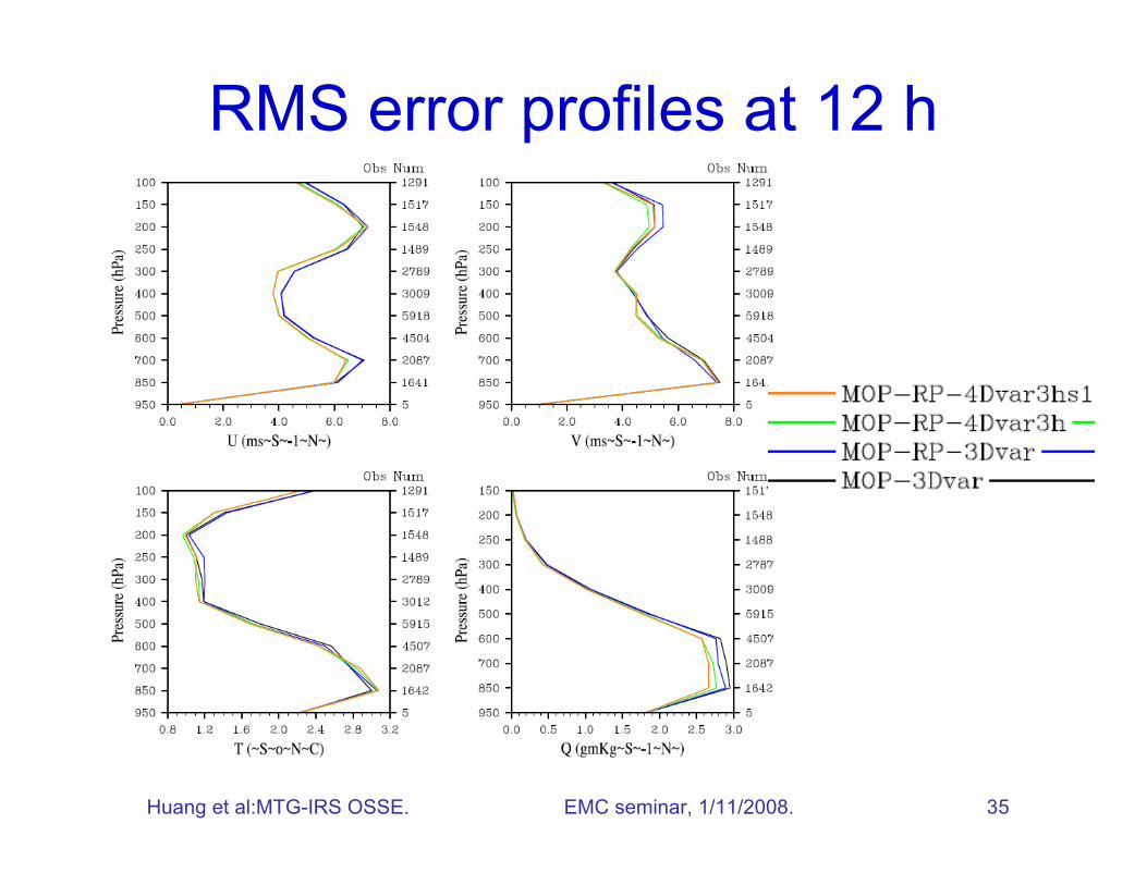
RMS error profiles at 12 hFCST
Huang et al:MTG-IRS OSSE. EMC seminar, 1/11/2008. 36
Summary
• Three storms are well reproduced in the 5 day nature run.
• The calibration experiment shows that the real and simulatedobservations have the similar impacts on the analysesincrements and forecasts differences.
• The quality of the retrievals has been improved significantly.
• The forecast skill is improved when MTG-IRS T and qretrieved profiles are assimilated.
Huang et al:MTG-IRS OSSE. EMC seminar, 1/11/2008. 37
Future work
• WRF-4DVAR experiments– Cycling assimilation and forecast experiments
– Time and computer source permitted
• Reduction of error correlations in MTG-IRS T(p) and q(p)
• Assimilating modeled wind observations from other
platforms (such as wind profilers or radars)
• OSSE for European cases.– Two nature runs have been carried out
Huang et al:MTG-IRS OSSE. EMC seminar, 1/11/2008. 38
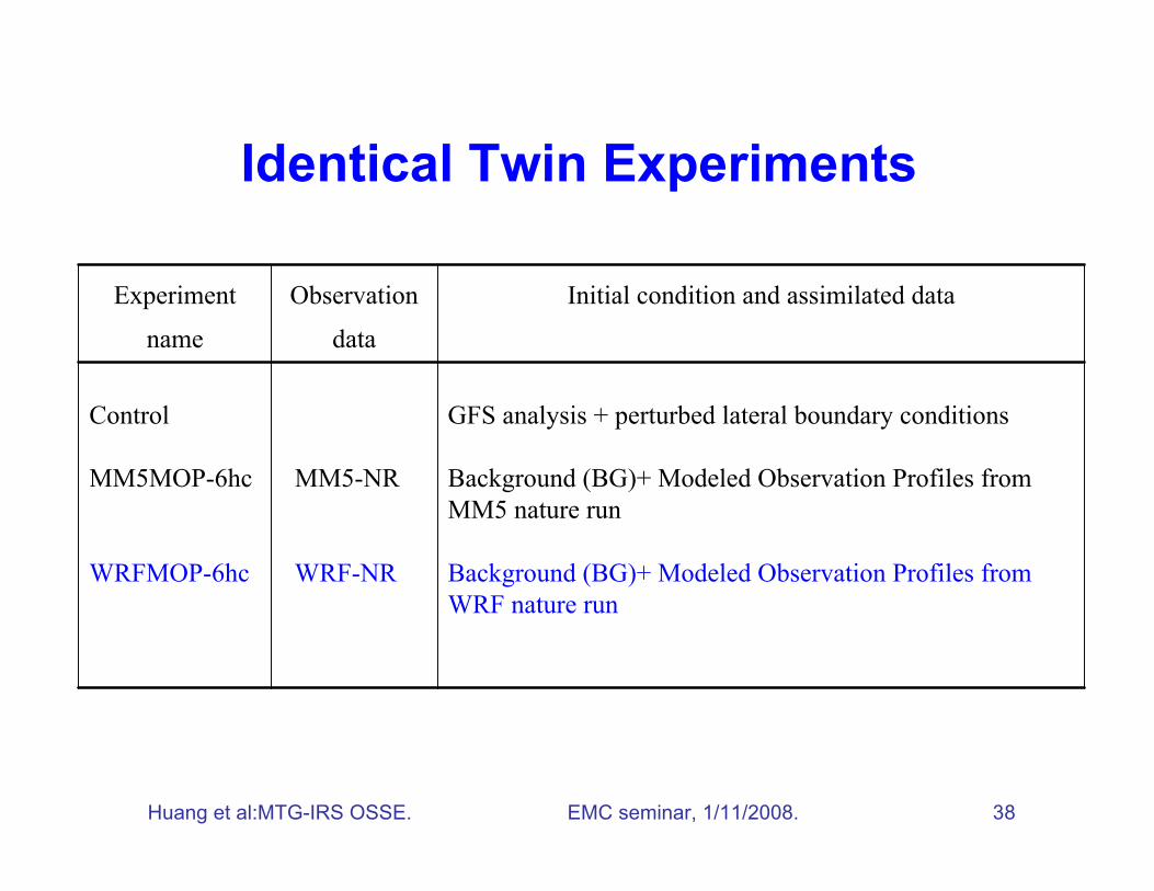
Identical Twin Experiments
GFS analysis + perturbed lateral boundary conditions
Background (BG)+ Modeled Observation Profiles fromMM5 nature run
Background (BG)+ Modeled Observation Profiles fromWRF nature run
MM5-NR
WRF-NR
Control
MM5MOP-6hc
WRFMOP-6hc
Initial condition and assimilated dataObservation
data
Experiment
name
Huang et al:MTG-IRS OSSE. EMC seminar, 1/11/2008. 39
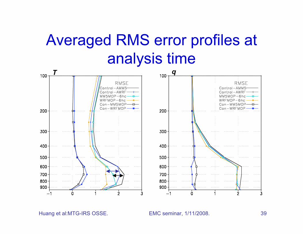
Averaged RMS error profiles atanalysis time
T q
Huang et al:MTG-IRS OSSE. EMC seminar, 1/11/2008. 40
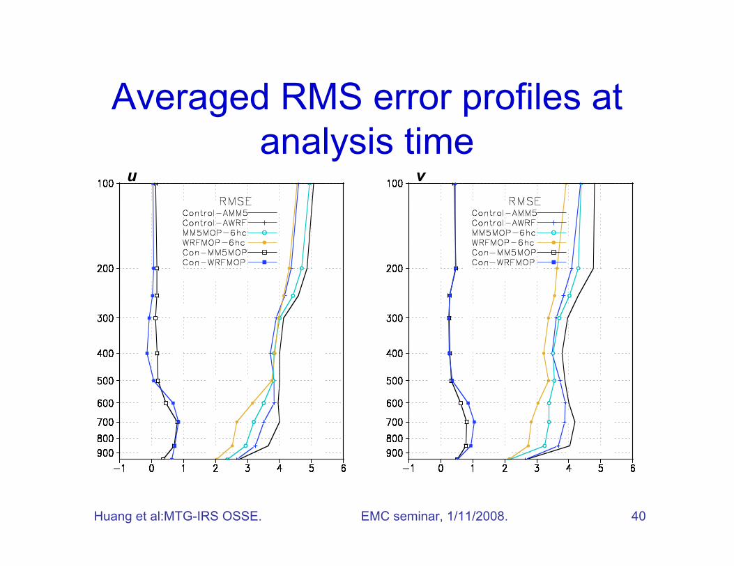
Averaged RMS error profiles atanalysis time
u v
Huang et al:MTG-IRS OSSE. EMC seminar, 1/11/2008. 41
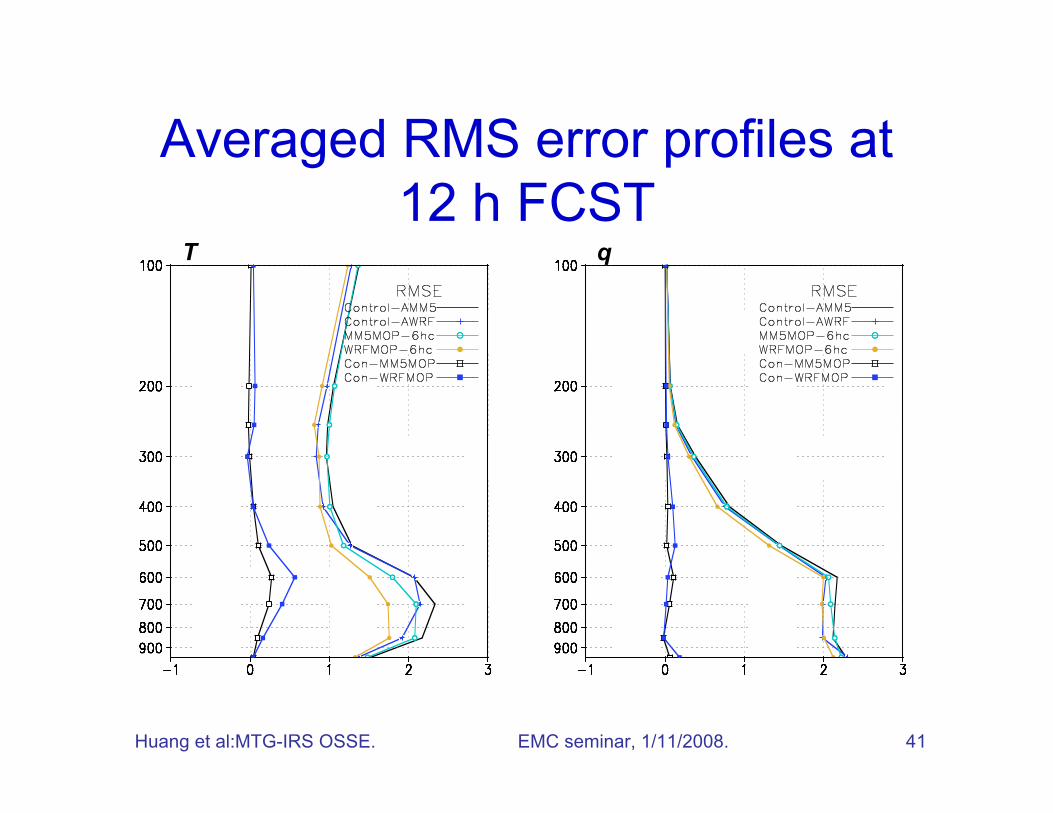
Averaged RMS error profiles at12 h FCST
T q
Huang et al:MTG-IRS OSSE. EMC seminar, 1/11/2008. 42
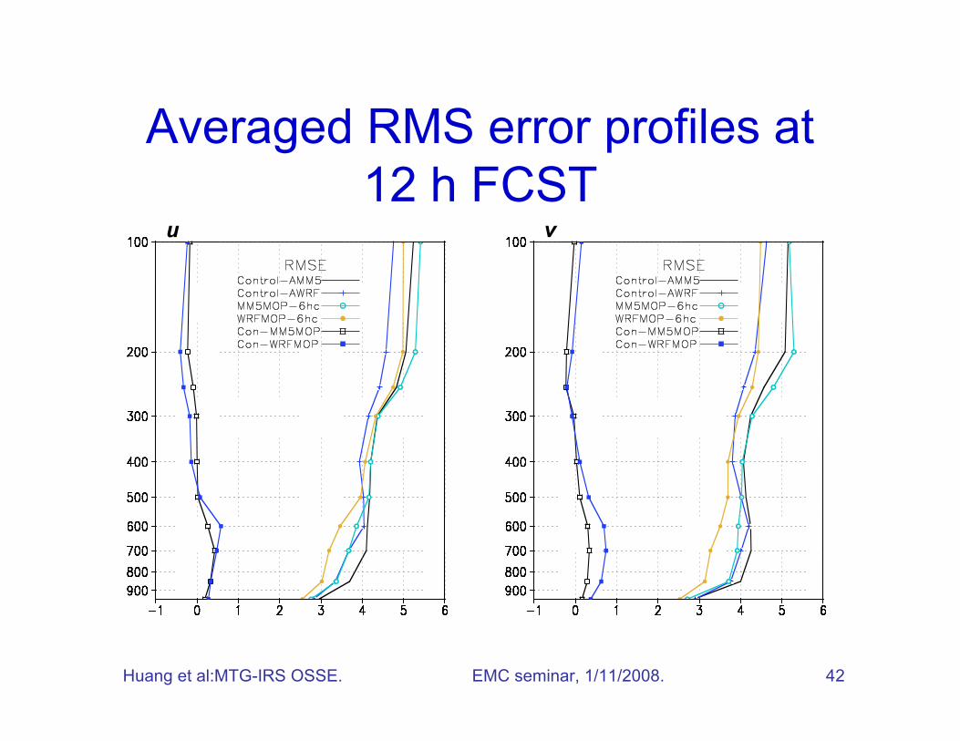
Averaged RMS error profiles at12 h FCST
u v
Huang et al:MTG-IRS OSSE. EMC seminar, 1/11/2008. 43
Compared with “non-identical”twin experiments
• The control experiment has smallererrors.
• The observation impact is larger.• Identical-twin experiments are not too
bad … may still be useful?!