MTAT.03.231 Business Process Management (BPM) Lecture 6 ... - ttu.eecloud.ld.ttu.ee/idu0111/Portals/0/Loengud/ITlecture6Dumas.pdf · MTAT.03.231 Business Process Management (BPM)

MTAT.03.231

Business Process Management (BPM)

Lecture 6

Quantitative Process Analysis

(Queuing & Simulation)

Marlon Dumas

marlon.dumas ät ut . ee

2

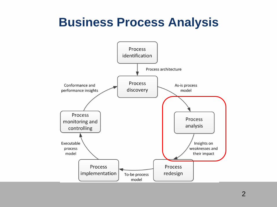
Business Process Analysis

3

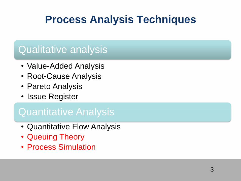
Process Analysis Techniques

Qualitative analysis

• Value-Added Analysis

• Root-Cause Analysis

• Pareto Analysis

• Issue Register

Quantitative Analysis

• Quantitative Flow Analysis

• Queuing Theory

• Process Simulation

4

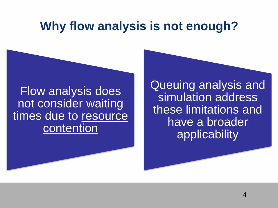
Why flow analysis is not enough?

Flow analysis does not consider waiting

times due to resource contention

Queuing analysis and simulation address

these limitations and have a broader

applicability

5

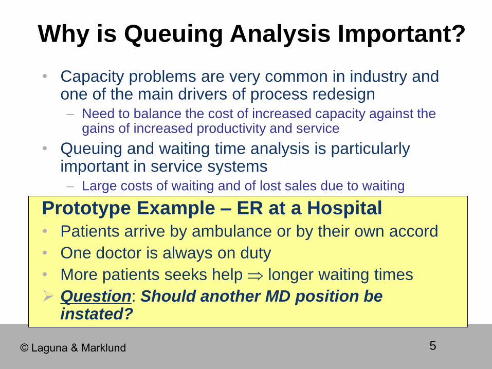
• Capacity problems are very common in industry and one of the main drivers of process redesign – Need to balance the cost of increased capacity against the

gains of increased productivity and service

• Queuing and waiting time analysis is particularly important in service systems – Large costs of waiting and of lost sales due to waiting

Prototype Example – ER at a Hospital • Patients arrive by ambulance or by their own accord

• One doctor is always on duty

• More patients seeks help longer waiting times

Question: Should another MD position be instated?

Why is Queuing Analysis Important?

© Laguna & Marklund

6

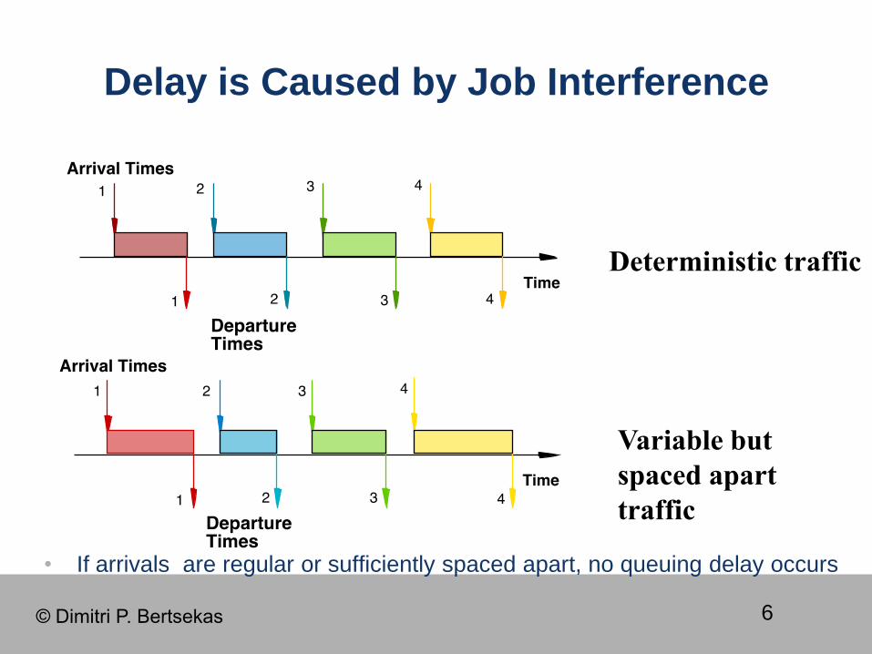
Delay is Caused by Job Interference

• If arrivals are regular or sufficiently spaced apart, no queuing delay occurs

Deterministic traffic

Variable but

spaced apart

traffic

© Dimitri P. Bertsekas

7

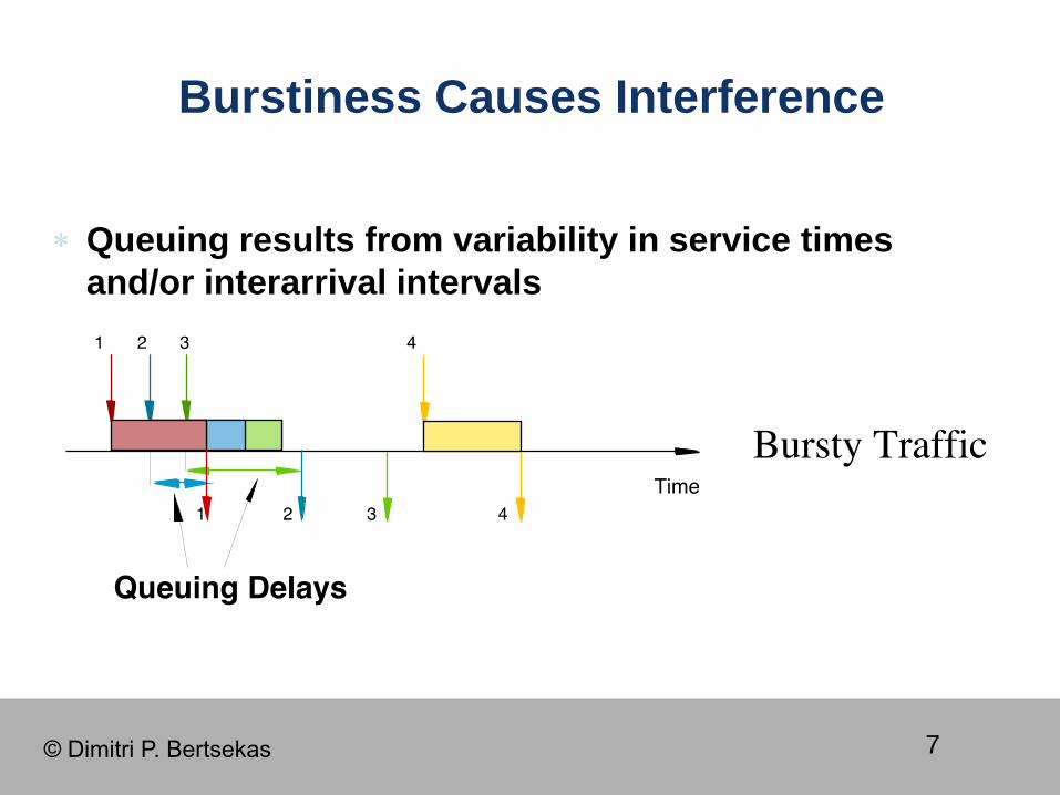
Burstiness Causes Interference

Queuing results from variability in service times

and/or interarrival intervals


8

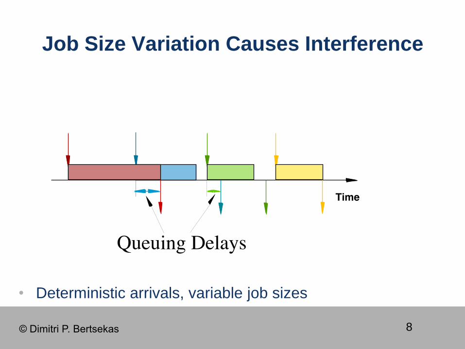
Job Size Variation Causes Interference

• Deterministic arrivals, variable job sizes


9

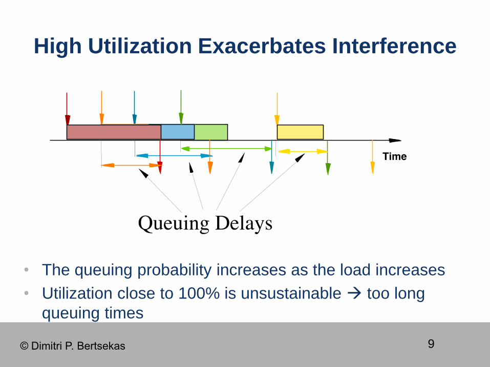
High Utilization Exacerbates Interference

• The queuing probability increases as the load increases

• Utilization close to 100% is unsustainable too long

queuing times


10

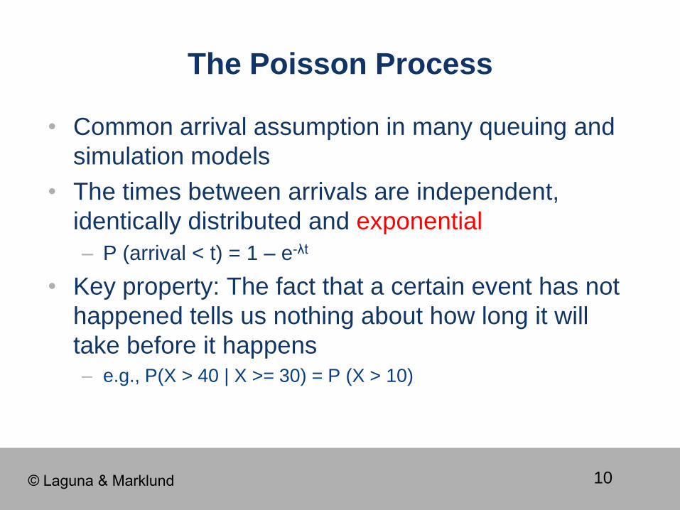
The Poisson Process

• Common arrival assumption in many queuing and

simulation models

• The times between arrivals are independent,

identically distributed and exponential

– P (arrival < t) = 1 – e-λt

• Key property: The fact that a certain event has not

happened tells us nothing about how long it will

take before it happens – e.g., P(X > 40 | X >= 30) = P (X > 10)


11

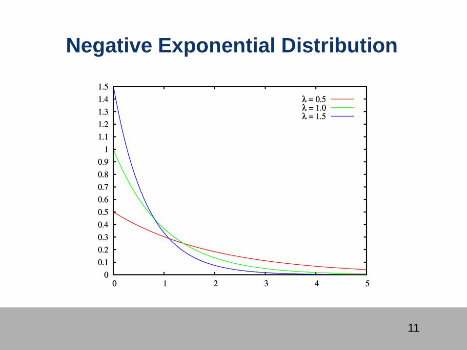
Negative Exponential Distribution

12

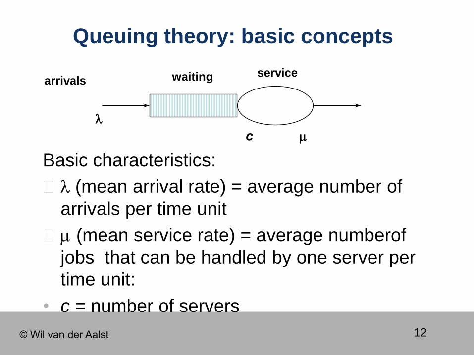
Queuing theory: basic concepts

Basic characteristics:

l (mean arrival rate) = average number of

arrivals per time unit

m (mean service rate) = average numberof

jobs that can be handled by one server per

time unit:

• c = number of servers

arrivals waiting service

l

m c

© Wil van der Aalst

13

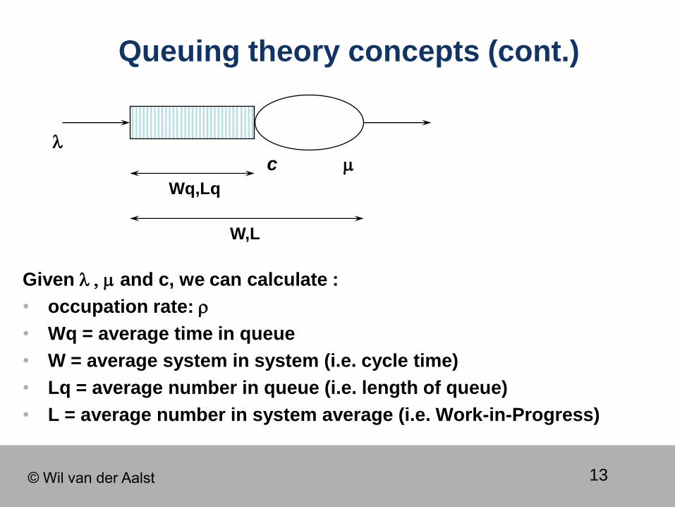
Queuing theory concepts (cont.)

Given l , m and c, we can calculate :

• occupation rate: r

• Wq = average time in queue

• W = average system in system (i.e. cycle time)

• Lq = average number in queue (i.e. length of queue)

• L = average number in system average (i.e. Work-in-Progress)

l

m c

Wq,Lq

W,L

© Wil van der Aalst

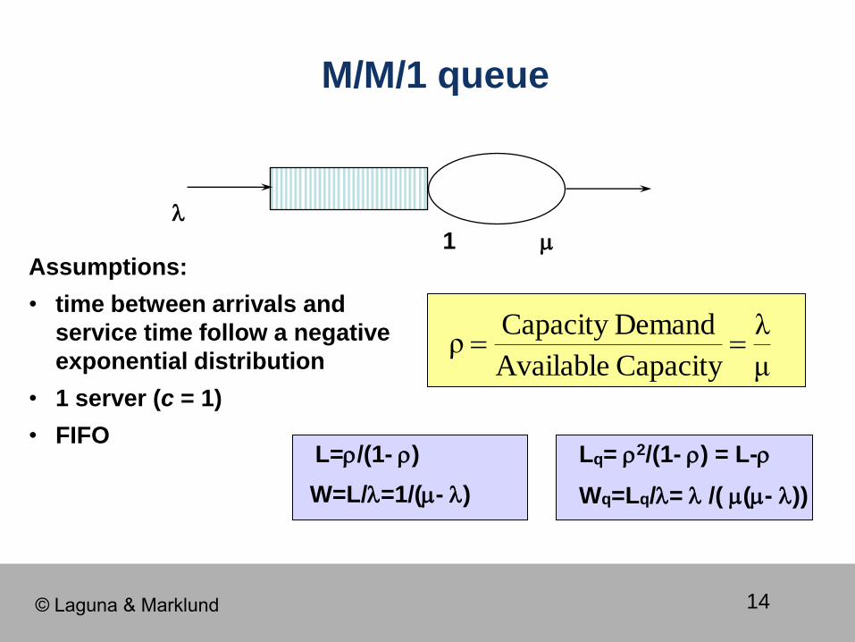
14

M/M/1 queue

l

m 1 Assumptions:

• time between arrivals and

service time follow a negative

exponential distribution

• 1 server (c = 1)

• FIFO L=r/(1- r) Lq= r2/(1- r) = L-r

W=L/l=1/(m- l) Wq=Lq/l= l /( m(m- l))

μ

λ

CapacityAvailable

DemandCapacityρ


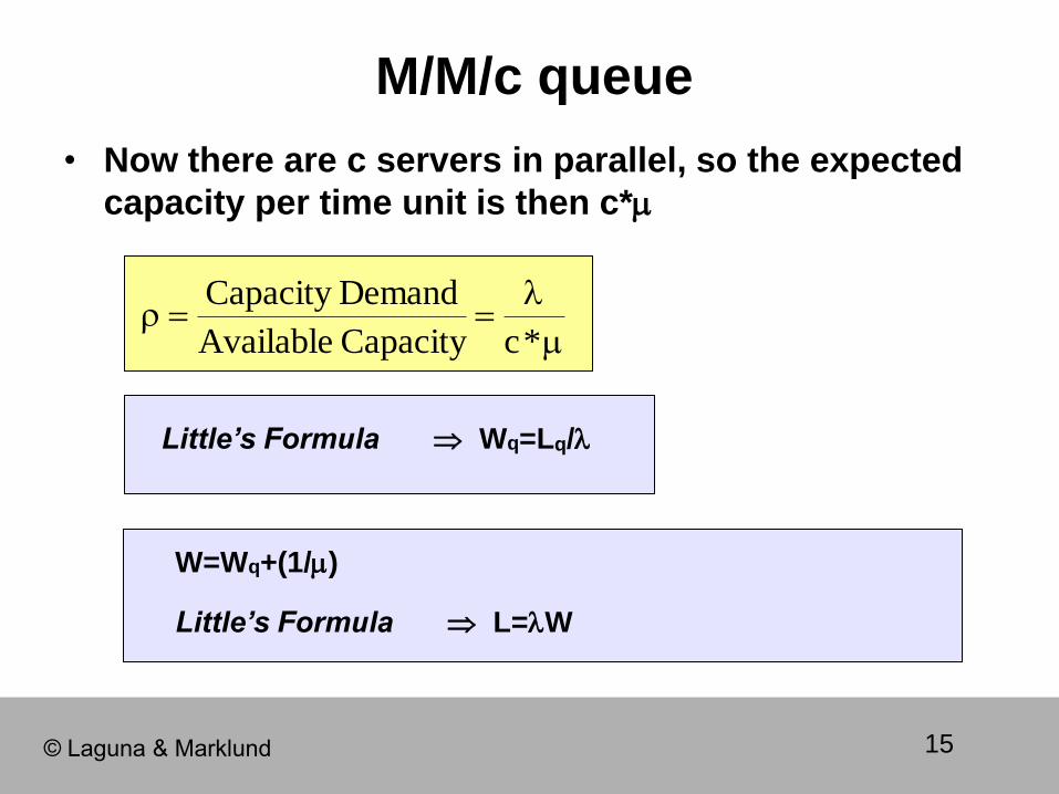
15

M/M/c queue

m

lr

*cCapacityAvailable

DemandCapacity

• Now there are c servers in parallel, so the expected

capacity per time unit is then c*m

W=Wq+(1/m)

Little’s Formula Wq=Lq/l

Little’s Formula L=lW


16

Tool Support

• For M/M/c systems, the exact computation of Lq is

rather complex…

• Consider using a tool, e.g.

– http://apps.business.ualberta.ca/aingolfsson/qtp/

– http://www.stat.auckland.ac.nz/~stats255/qsim/qsim.html

02

c

cnnq P

)1(!c

)/(...P)cn(L

r

rml

1c1c

0n

n

0)c/((1

1

!c

)/(

!n

)/(P

ml

ml

ml

http://apps.business.ualberta.ca/aingolfsson/qtp/

http://www.stat.auckland.ac.nz/~stats255/qsim/qsim.html

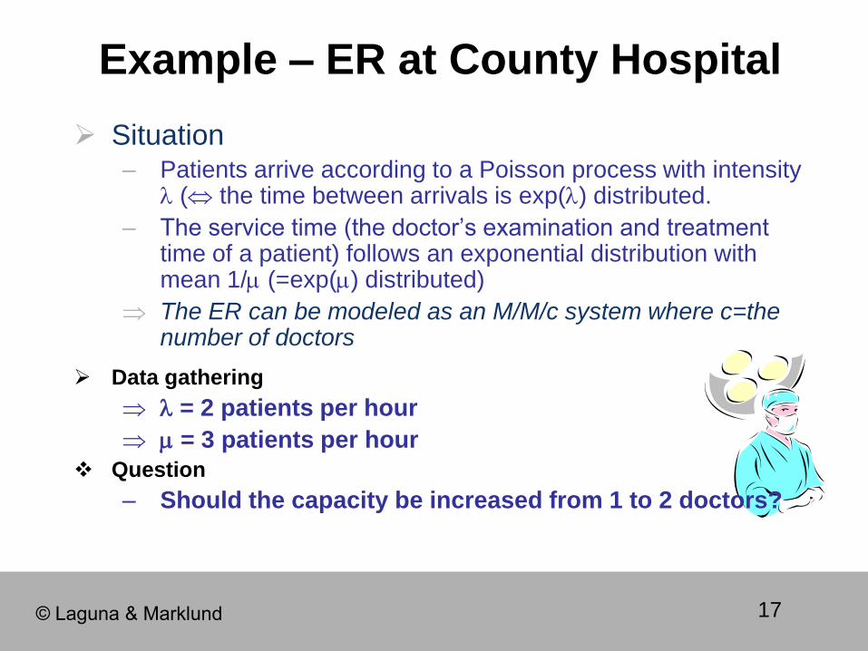
17

Situation – Patients arrive according to a Poisson process with intensity

l ( the time between arrivals is exp(l) distributed.

– The service time (the doctor’s examination and treatment time of a patient) follows an exponential distribution with mean 1/m (=exp(m) distributed)

The ER can be modeled as an M/M/c system where c=the number of doctors

Example – ER at County Hospital

Data gathering

l = 2 patients per hour

m = 3 patients per hour

Question

– Should the capacity be increased from 1 to 2 doctors?


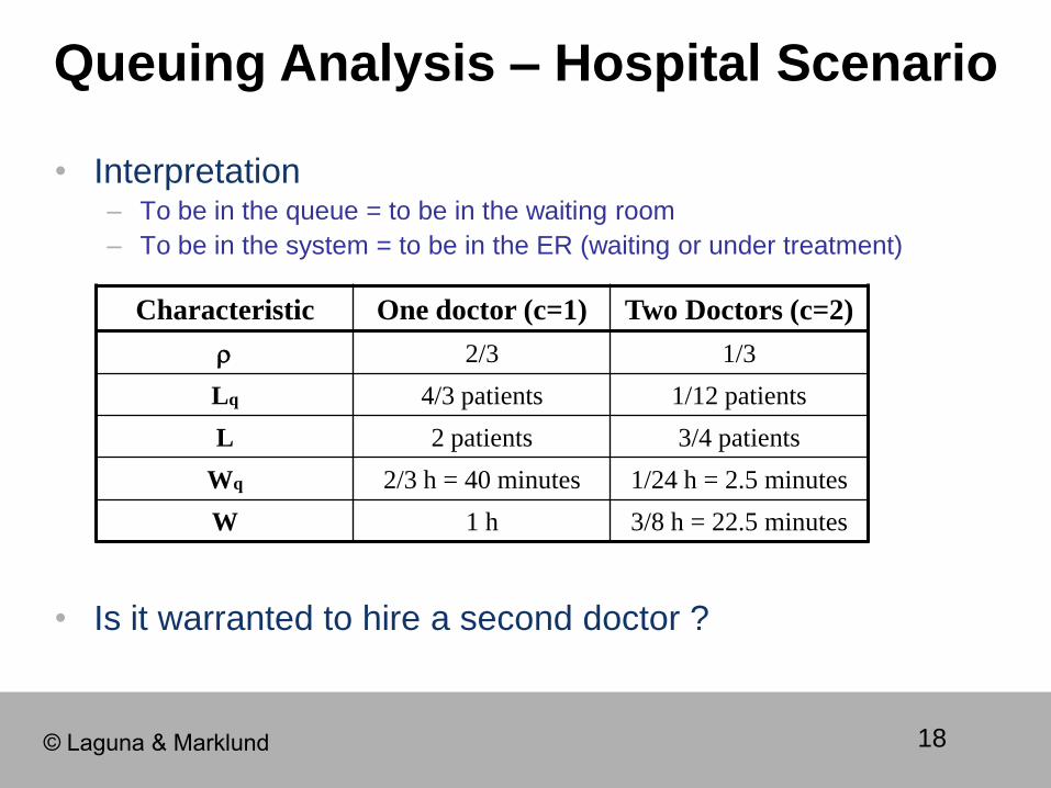
18

• Interpretation – To be in the queue = to be in the waiting room

– To be in the system = to be in the ER (waiting or under treatment)

• Is it warranted to hire a second doctor ?

Queuing Analysis – Hospital Scenario

Characteristic One doctor (c=1) Two Doctors (c=2)

r 2/3 1/3

Lq 4/3 patients 1/12 patients

L 2 patients 3/4 patients

Wq 2/3 h = 40 minutes 1/24 h = 2.5 minutes

W 1 h 3/8 h = 22.5 minutes


19

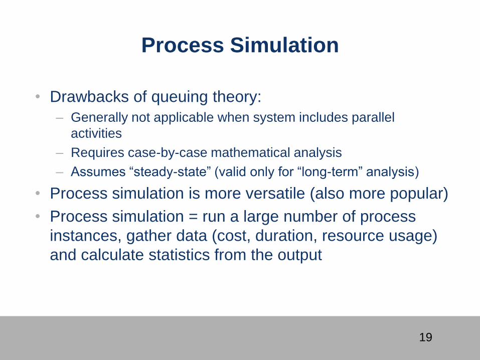
• Drawbacks of queuing theory:

– Generally not applicable when system includes parallel

activities

– Requires case-by-case mathematical analysis

– Assumes “steady-state” (valid only for “long-term” analysis)

• Process simulation is more versatile (also more popular)

• Process simulation = run a large number of process

instances, gather data (cost, duration, resource usage)

and calculate statistics from the output

Process Simulation

20

Process Simulation

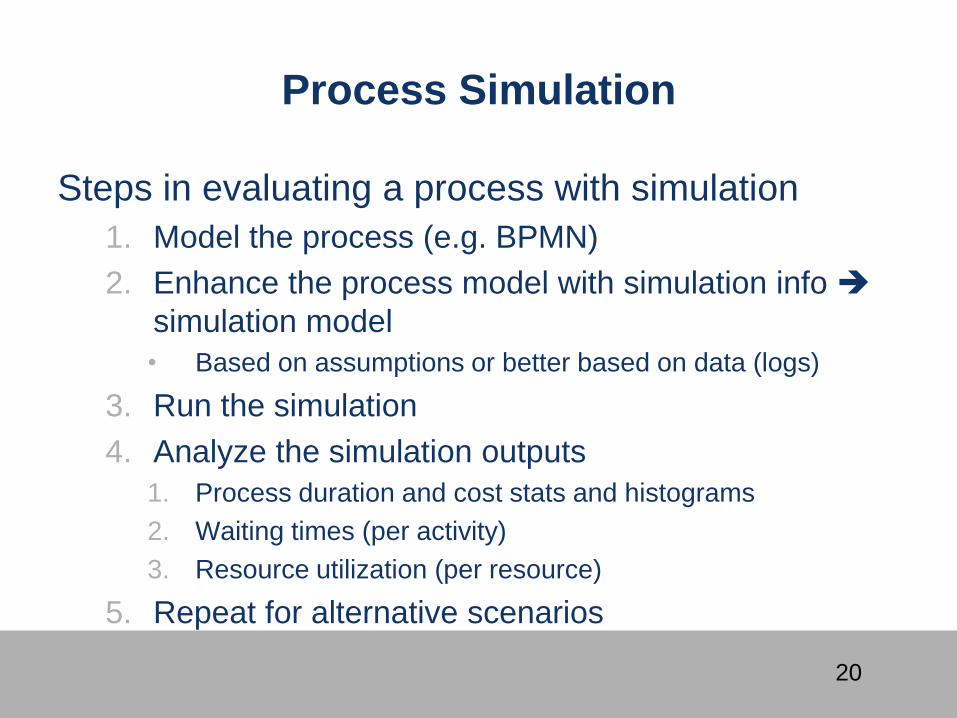
Steps in evaluating a process with simulation

1. Model the process (e.g. BPMN)

2. Enhance the process model with simulation info

simulation model

• Based on assumptions or better based on data (logs)

3. Run the simulation

4. Analyze the simulation outputs

1. Process duration and cost stats and histograms

2. Waiting times (per activity)

3. Resource utilization (per resource)

5. Repeat for alternative scenarios

21

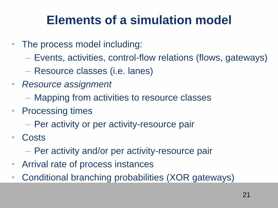
Elements of a simulation model

• The process model including:

– Events, activities, control-flow relations (flows, gateways)

– Resource classes (i.e. lanes)

• Resource assignment

– Mapping from activities to resource classes

• Processing times

– Per activity or per activity-resource pair

• Costs

– Per activity and/or per activity-resource pair

• Arrival rate of process instances

• Conditional branching probabilities (XOR gateways)

22

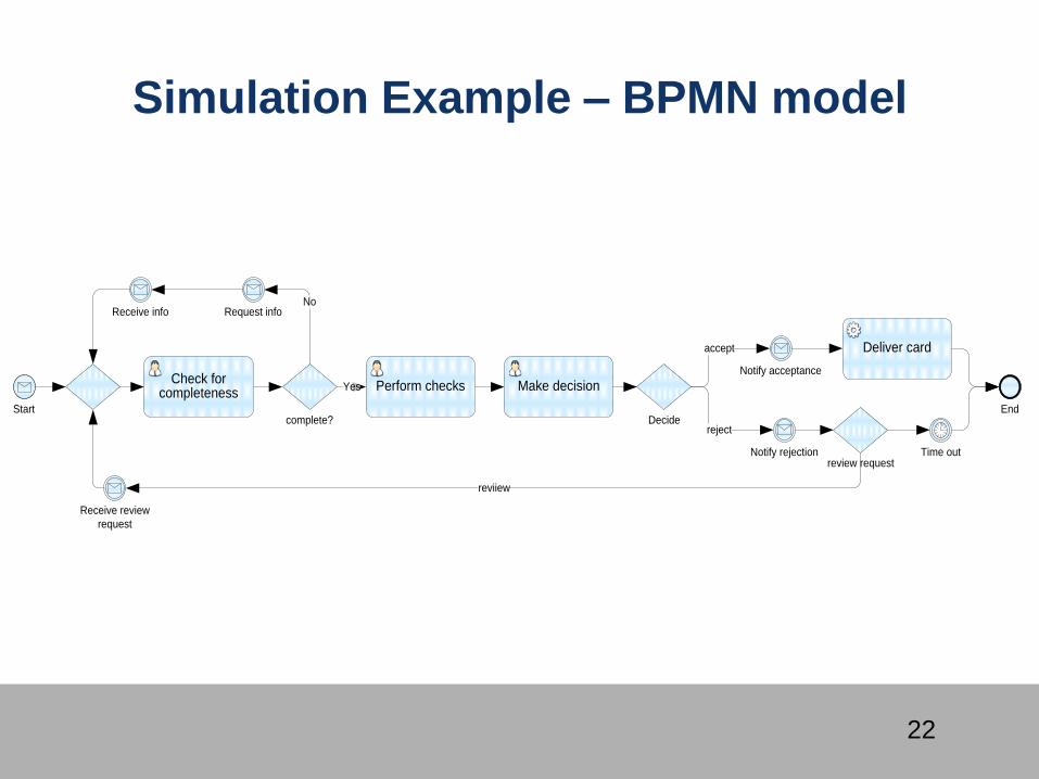
Simulation Example – BPMN model

Start End

Check for completeness

Perform checks Make decision

Deliver card

Receive review

request

Request infoReceive info

Notify acceptance

Notify rejection Time out

complete? Decide

review request

Yes

No

reject

reviiew

accept

23

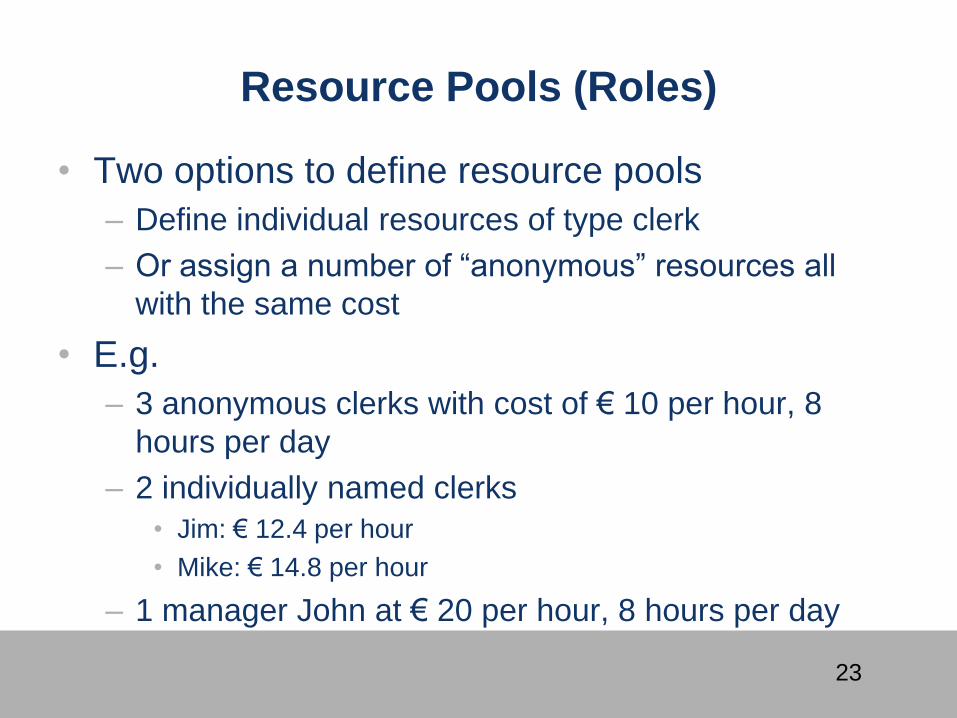
Resource Pools (Roles)

• Two options to define resource pools

– Define individual resources of type clerk

– Or assign a number of “anonymous” resources all

with the same cost

• E.g.

– 3 anonymous clerks with cost of € 10 per hour, 8

hours per day

– 2 individually named clerks

• Jim: € 12.4 per hour

• Mike: € 14.8 per hour

– 1 manager John at € 20 per hour, 8 hours per day

24

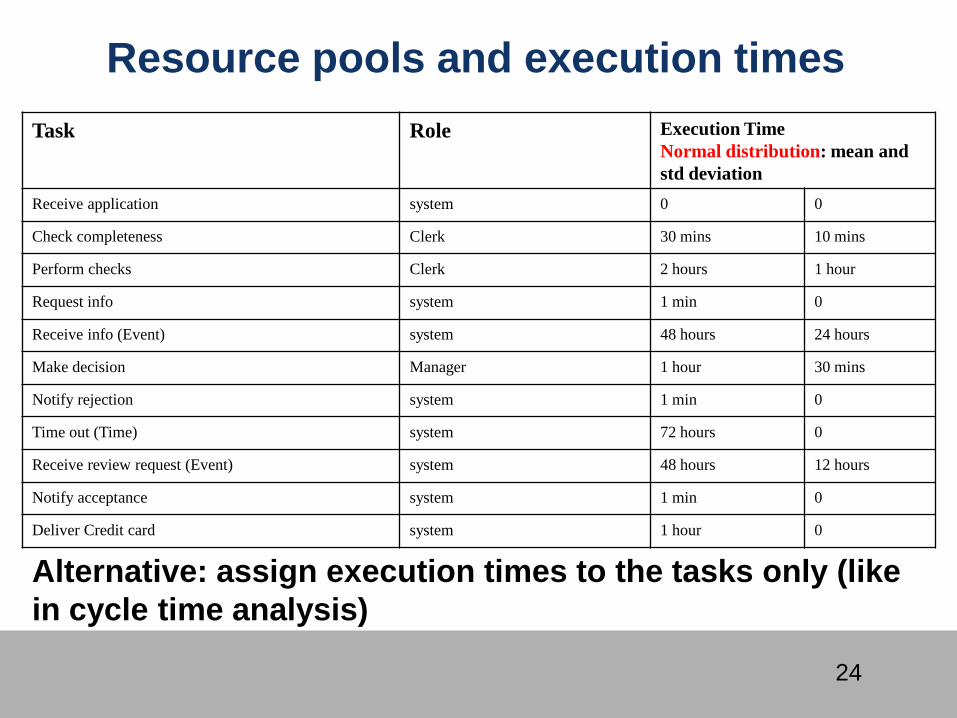
Resource pools and execution times

Task Role Execution Time

Normal distribution: mean and

std deviation

Receive application system 0 0

Check completeness Clerk 30 mins 10 mins

Perform checks Clerk 2 hours 1 hour

Request info system 1 min 0

Receive info (Event) system 48 hours 24 hours

Make decision Manager 1 hour 30 mins

Notify rejection system 1 min 0

Time out (Time) system 72 hours 0

Receive review request (Event) system 48 hours 12 hours

Notify acceptance system 1 min 0

Deliver Credit card system 1 hour 0

Alternative: assign execution times to the tasks only (like

in cycle time analysis)

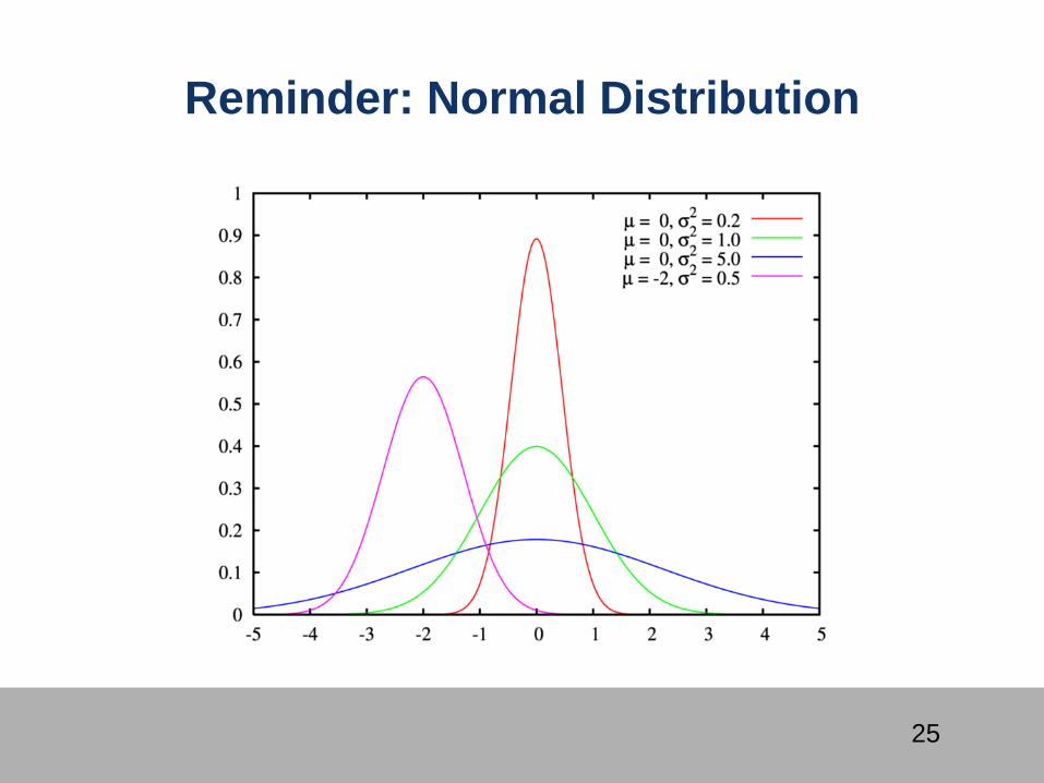
25

Reminder: Normal Distribution

26

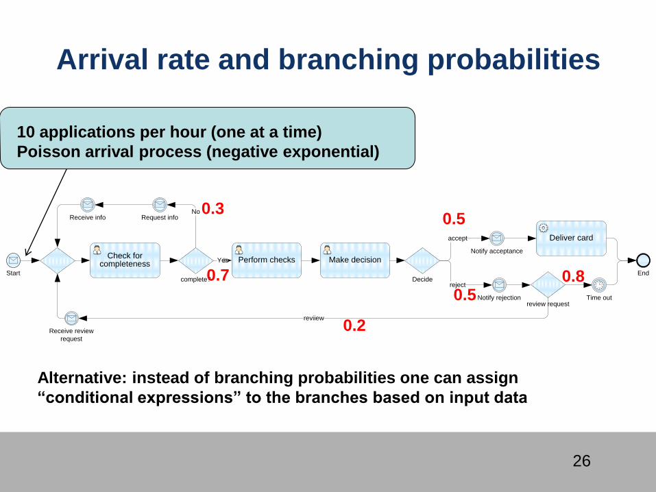
Arrival rate and branching probabilities

Start End

Check for completeness

Perform checks Make decision

Deliver card

Receive review

request

Request infoReceive info

Notify acceptance

Notify rejection Time out

complete? Decide

review request

Yes

No

reject

reviiew

accept

10 applications per hour (one at a time)

Poisson arrival process (negative exponential)

0.5

0.7

0.3

0.5

Alternative: instead of branching probabilities one can assign

“conditional expressions” to the branches based on input data

0.2

0.8

27

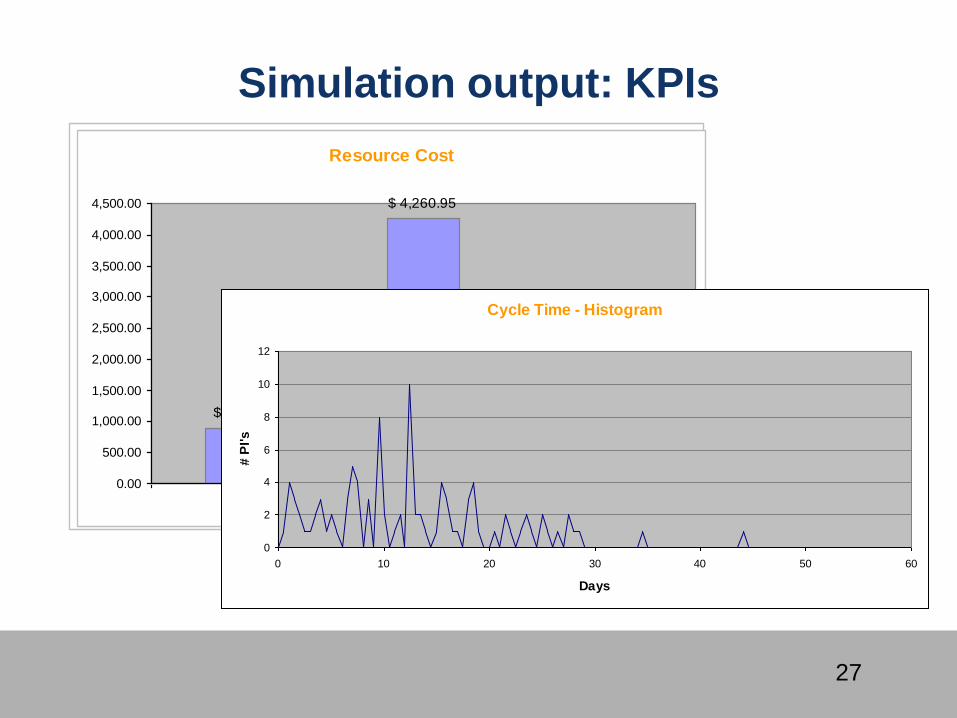
Simulation output: KPIs

Resource Utilization

18.82%

50.34%

5.04%

0.00%

10.00%

20.00%

30.00%

40.00%

50.00%

60.00%

70.00%

80.00%

90.00%

100.00%

Clerk Manager System

Resource Cost

$ 898.45

$ 4,260.95

$ 285.00

0.00

500.00

1,000.00

1,500.00

2,000.00

2,500.00

3,000.00

3,500.00

4,000.00

4,500.00

Clerk Manager System

Cycle Time - Histogram

0

2

4

6

8

10

12

0 10 20 30 40 50 60

Days

# P

I's

28

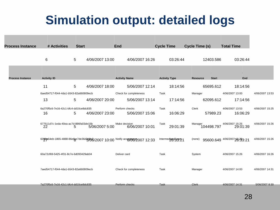
Simulation output: detailed logs

Process Instance # Activities Start End Cycle Time Cycle Time (s) Total Time

6 5 4/06/2007 13:00 4/06/2007 16:26 03:26:44 12403.586 03:26:44

7 5 4/06/2007 14:00 5/06/2007 9:30 19:30:38 70238.376 19:30:38

11 5 4/06/2007 18:00 5/06/2007 12:14 18:14:56 65695.612 18:14:56

13 5 4/06/2007 20:00 5/06/2007 13:14 17:14:56 62095.612 17:14:56

16 5 4/06/2007 23:00 5/06/2007 15:06 16:06:29 57989.23 16:06:29

22 5 5/06/2007 5:00 6/06/2007 10:01 29:01:39 104498.797 29:01:39

27 8 5/06/2007 10:00 6/06/2007 12:33 26:33:21 95600.649 26:33:21

Process Instance Activity ID Activity Name Activity Type Resource Start End

6 aed54717-f044-4da1-b543-82a660809ecb Check for completeness Task Manager 4/06/2007 13:00 4/06/2007 13:53

6 a270f5c6-7e16-42c1-bfc4-dd10ce8dc835 Perform checks Task Clerk 4/06/2007 13:53 4/06/2007 15:25

6 77511d7c-1eda-40ea-ac7d-886fa03de15b Make decision Task Manager 4/06/2007 15:25 4/06/2007 15:26

6 099a64eb-1865-4888-86e6-e7de36d348c2 Notify acceptance IntermediateEvent (none) 4/06/2007 15:26 4/06/2007 15:26

6 0a72cf69-5425-4f31-8c7e-6d093429ab04 Deliver card Task System 4/06/2007 15:26 4/06/2007 16:26

7 aed54717-f044-4da1-b543-82a660809ecb Check for completeness Task Manager 4/06/2007 14:00 4/06/2007 14:31

7 a270f5c6-7e16-42c1-bfc4-dd10ce8dc835 Perform checks Task Clerk 4/06/2007 14:31 5/06/2007 8:30

29

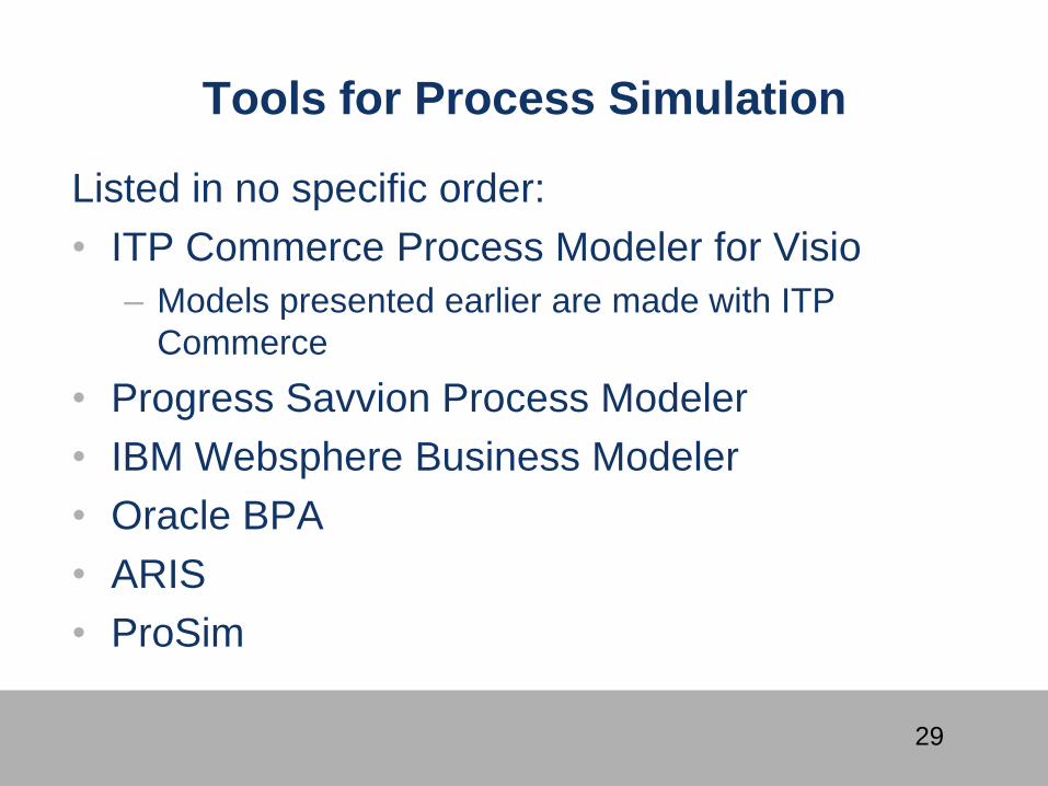
Tools for Process Simulation

Listed in no specific order:

• ITP Commerce Process Modeler for Visio

– Models presented earlier are made with ITP

Commerce

• Progress Savvion Process Modeler

• IBM Websphere Business Modeler

• Oracle BPA

• ARIS

• ProSim

30

Simple Online Simulator

• BIMP: http://bimp.cs.ut.ee/

• Accepts standard BPMN 2.0 as input

• Link from Signavio Academic Edition to BIMP

– Open a model in Signavio and push it to BIMP using

the flask icon

http://bimp.cs.ut.ee/

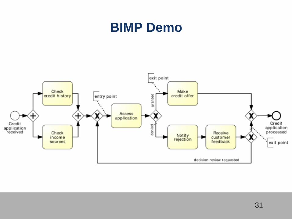
31

BIMP Demo

Documents

MTAT.03.231 Business Process Management (BPM) Lecture 6 ... - ttu.eecloud.ld.ttu.ee/idu0111/Portals/0/Loengud/ITlecture6Dumas.pdf · MTAT.03.231 Business Process Management (BPM)