MSc Mas6002 Introductory Material

Block A

Introduction to Probability and Statistics

1 Probability

1.1 Multiple approaches

The concept of probability may be defined and interpreted in several different ways, the

chief ones arising from the following four approaches.

1.1.1 The classical approach

A game of chance has a finite number of different possible outcomes, which by symmetry

are assumed ‘equally likely’. The probability of any event (i.e. particular outcome of

interest) is then defined as the proportion of the total number of possible outcomes for

which that event does occur.

Evaluating probabilities in this framework involves counting methods (e.g. permutations

and combinations).

1.1.2 The frequency approach

An experiment can be repeated indefinitely under essentially identical conditions, but

the observed outcome is random (not the same every time). Empirical evidence suggests

that the proportion of times any particular event has occurred, i.e. its relative frequency,

converges to a limit as the number of repetitions increases. This limit is called the

probability of the event.

1.1.3 The subjective approach

In this approach, an event is a statement which may or may not be true, and the (sub-

jective) probability of the event is a measure of the degree of belief which the subject has

in the truth of the statement. If we imagine that a ‘prize’ is available if and only if the

statement does turn out to be true, the subjective probability can be thought of as the

proportion of the prize money which the subject is prepared to gamble in the hope of

winning the prize.

1.1.4 The logical approach

Formal logic depends on relationships of the kind A −→ B (‘A implies B’) between

propositions. The logical approach to probability generalizes the concept of implication

1

to partial implication; the conditional probability of B given A measures the extent to

which A implies B. In this approach, all probabilities are ‘conditional’; there are no

‘absolute’ probabilities.

Some pros and cons of the four approaches:

Classical Frequency Subjective Logical

Calculation Objective and Applicable to Extends formal

PRO straight-forward empirical wide range logic in

of ‘events’ consistent way

Limited Depends on Depends on Yields no way

CON in scope infinite individual of assigning

repeatability probabilities

1.2 Axiomatic probability theory

Because there is not a uniquely best way of defining probabilities, it is customary to lay

down a set of rules (axioms) which we expect probabilities to obey (whichever interpre-

tation is put on them). A mathematical theory can then be developed from these rules.

The framework is as follows. For any probability model we require a probability space

(Ω, F, P ) with

• the set Ω of all possible outcomes, known as the sample space (for the game, exper-

iment, etc.)

• a collection F of subsets of Ω, each subset being called an event (i.e. the event that

the observed outcome lies in that subset).

• a probability measure defined as a real valued function P of the elements of F (the

events) satisfying the following axioms of probability:

A1 P (A) ≥ 0 for all A ∈ FA2 P (Ω) = 1

A3 If A1, A2,... are mutually exclusive events (i.e. have no elements in common),

then P (A1∪A2∪ ...) = P (A1) +P (A2) + ... [The sum may be finite or infinite].

Example 1. In a ‘classical’ probability model, Ω consists of the n equally likely outcomes

a1, a2, ..., an say, F consists of all subsets of Ω, and P is defined by

P (A) =no. of elements in A

nfor A ∈ F.

It is easy to show that the P satisfies the axioms of probability.

Theorems about probabilities may be proved using the axioms. The following is a simple

example.

Theorem 1. If Ac = Ω\A, (the ‘complement’ or ‘negation’ of A), then P (Ac) = 1−P (A).

2

Proof. A and Ac are mutually exclusive with union Ω. Therefore

P (A) + P (Ac) = P (Ω) (by axiom A3)

= 1 (by axiom A2).

1.3 Conditional probability

For any event A with P (A) > 0, we can ‘condition’ on the occurrence of A by defining

a new probability measure, PA say, which is obtained from P by reducing all probability

outside A to zero and rescaling the rest so that the axioms are still satisfied. Thus for

any event B in the original sample space Ω, we define

PA(B) =P (A ∩B)

P (A)= probability of B conditional on A or given A

PA(B) is normally written P (B | A).

Conditional probabilities are often easier to specify than unconditional ones, and the

above definition may be rearranged to give

P (A ∩B) = P (A)P (B | A)

which is sometimes known as the multiplication rule. This may be extended (by an easy

induction argument) to a sequence A1, A2, ..., An of events

P (A1 ∩ A2 ∩ . . . ∩ An) = P (A1)P (A2 | A1)P (A3 | A1 ∩ A2) . . . P (An | A1 ∩ . . . ∩ An−1)

which is useful when it is easy to write down the probability of each event in the sequence

conditional on all the previous ones having occurred.

Another important relationship involving conditional probabilities is the law of total prob-

ability (sometimes known as the elimination rule). This involves the notion of a partition

of the sample space, which is a sequence A1, A2, . . . (finite or infinite) such that

A1 ∪ A2 ∪ . . . = Ω

and Ai ∩ Aj = φ whenever i 6= j. In other words, ‘A1, A2, . . . are mutually exclusive and

exhaustive’ or alternatively ‘one and only one of A1, A2, . . . must occur’. If A1, A2, . . . is

a partition and B is an arbitrary event, then the law of total probability states that

P (B) =∑i

P (Ai)P (B | Ai)

This follows from the axioms and the definition of conditional probability, since A1 ∩B,A2 ∩B, . . . are mutually exclusive with union B, and P (Ai ∩B) = P (Ai)P (B | Ai) for

each i.

Example 2. In a multiple choice test, each question has m possible answers. If a candi-

date knows the right answer (which happens with probability p) he gives it; if he thinks

he knows it but is mistaken (which has probability q) he gives the answer he thinks is

3

correct; and if he does not think he knows it (with probability r = 1 − p − q) then he

chooses an answer at random. What is the probability that he answers correctly?

Let A1 be the event that the candidate knows the right answer, A2 the event that he

thinks he knows it but is mistaken, and A3 the event that he does not think he knows it.

Let B be the event that he answers correctly.

P (A1) = p P (B | A1) = 1

P (A2) = q P (B | A2) = 0

P (A3) = r P (B | A3) = 1/m

therefore

P (B) = p× 1 + q × 0 + r × 1

m= p+

r

m.

Sometimes we wish to relate two conditional probabilities. This is easily achieved

P (A | B) =P (B ∩ A)

P (B)=P (A ∩B)

P (B)=P (B | A)P (A)

P (B)

This result is known as Bayes’ Theorem (or Bayes’ rule). It is often used in conjunction

with a partition where we wish to know the probability of one (or more) of the events of

the partition having occurred conditional on the ‘secondary event’ B having been observed

to occur:

P (Aj | B) =P (Aj)P (B | Aj)

P (B)=

P (Aj)P (B | Aj)ΣP (Ai)P (B | Ai)

Example 3. (Model as above). What is the probability that the candidate knew the

right answer given that he answered correctly?

P (A1 | B) =p× 1

p× 1 + q × 0 + r × 1m

=p

p+ rm

Bayes’ Theorem lies at the foundation of a whole branch of statistics – Bayesian statistics.

See MAS6004.

1.4 Independence

Event B is said to be independent of event A if

P (B | A) = P (B)

i.e. conditioning on A does not affect the probability of B. The relationship is more usually

written equivalently as

P (A ∩B) = P (A)P (B)

which indicates that the relationship is symmetrical: A and B are mutually indepen-

dent. This form my be generalized to longer sequences: events A1, A2, . . . are said to be

(mutually) independent if

P (Ai1 ∩ Ai2 ∩ . . . ∩ Aik) = P (Ai1)P (Ai2) . . . P (Aik)

for any finite collection of distinct subscripts i1, i2, . . . ik.

4

Example 4. For three events A, B, C to be mutually independent, all the following

relationships must hold:

P (A ∩B) = P (A)P (B)

P (A ∩ C) = P (A)P (C)

P (B ∩ C) = P (B)P (C)

P (A ∩B ∩ C) = P (A)P (B)P (C).

Fortunately, independence is usually used as an assumption in constructing probability

models, and so we do not need to check a whole collection of relationships such as the

above.

1.5 Worked examples

Example 5. Consider the roll of an ordinary six-sided die. Then the sample space Ω is

the set of outcomes, i.e. 1, 2, 3, 4, 5, 6.

Let A be the event that we roll an even number, and let B be the event that we roll at

least 4. As subsets of Ω, A = 2, 4, 6 and B = 4, 5, 6.

Now look at the various set operations applied to these two events:

• A ∪ B = 2, 4, 5, 6: we roll an even number or we roll at least 4. (NB inclusive

“or”: both 4 and 6 are included.)

• A ∩B = 4, 6: we roll an even number and we roll at least 4, i.e. we roll 4 or 6.

• Ac = 1, 3, 5: we do not roll an even number, i.e. we roll an odd one.

If the die is fair we can assume that the elements of Ω are equally likely. We can then

work out probabilities of events by simply counting the number of elements and dividing

by the total number of elements in Ω (here 6): P (A) = 3/6 = 1/2, P (B) = 3/6 = 1/2,

P (A ∪B) = 4/6 = 2/3, etc.

Example 6. A bag contains 8 balls labelled 1, 2, . . . , 8. Three balls are drawn randomly

without replacement. Calculate (a) the probability that the ball labelled 4 is drawn, (b)

the probability that the three balls drawn have consecutive numbers (e.g. 3,4,5). Are the

events in (a) and (b) independent?

The number of outcomes here is the number of ways of selecting 3 from 8, i.e.(

83

)= 56.

(The order that the balls are drawn in is not important; otherwise the number of outcomes

would be 8× 7× 6 = 336.) (a) If ball 4 is drawn, there are(

72

)= 21 possibilities for the

other two, so, given equally likely outcomes, the probability is 21/56 = 3/8. (b) There

are six outcomes here, so the probability is 6/56 = 3/28.

Call the events A and B respectively. Then A∩B requires the balls to be 2, 3, 4, 3, 4, 5or 4, 5, 6, and hence has probability 3/56. But P (A)P (B) = 9/224 6= 3/56, so the two

events are not independent. (The conditional probability P (A|B) = P (A ∩ B)/P (B) =

(3/56)/(3/28) = 1/2 > 3/8, so B occurring increases the chance of A occurring.)

5

2 Random variables

2.1 Definition

Often the outcome of an experiment will have numerical values, e.g. throwing a die we can

take the sample space to be Ω = 1, 2, 3, 4, 5, 6. In other more complicated experiments

even though the outcomes may not be numerical we may be interested in a numerical

value which is a function of the observed outcome, e.g. throwing three dice we may be

interested in ‘the total score obtained’. In this latter example, the sample space may be

described as

Ω = (1, 1, 1), (1, 1, 2), (1, 1, 3), . . . . . . (6, 6, 6)

but the possible values which ‘the total score obtained’ can take are given by

ΩX = 3, 4, 5, . . . 18

which is called the induced sample space. The function which takes Ω into ΩX according

to the rule described is called a random variable, e.g. ‘the total score obtained’ is a random

variable which we may call X say. Associated with the sample space induced by X are:

(i) FX = events ‘generated’ by X (e.g. ‘X=4’ and ‘X is an even number’ are events);

(ii) PX = induced probability measure, known as the distribution of X, e.g. PX(3, 4) =

P (X = 3 or 4) = P(1, 1, 1), (1, 1, 2), (1, 2, 1)(2, 1, 1) = 4216

assuming dice are fair.

It is often convenient to work with (ΩX , FX , PX), rather than with (Ω, F, P ), but we have

to be careful if considering more than one random variable defined on the same underlying

sample space.

2.2 Types of distribution

A random variable X, or its distribution, is called discrete if it only takes values in the

integers or (possibly) some other countable set of real numbers. (This will automatically

be true if the underlying sample space is countable.) In this case the distribution is

entirely specified by giving its value on every singleton in the induced sample space:

PX(i) = pX(i) for i ∈ ΩX .

pX(i) is called the probability function of X (or of its distribution). The probability of any

event AX in FX is then found by summing the values of pX over the singletons contained

in AX :

P (AX) =∑i∈AX

pX(i) (1)

In order to satisfy the axioms of probability, it is sufficient that the function pX satisfies

(i) pX(i) > 0 for all i ∈ ΩX (to satisfy A1)

(ii)∑

i∈ΩXpX(i) = 1 (to satisfy A2)

6

A3 is then automatically satisfied because of (1).

Example 7.

pX(i) =1

i(i+ 1)with ΩX = 1, 2, 3, . . .

is a probability function since pX(i) > 0 obviously and also

∞∑i=1

pX(i) =∞∑i=1

(1

i− 1

i+ 1

)= 1.

A random variable X, or its distribution, is called (absolutely) continuous if it takes values

on the whole real line or some sub-intervals and the probability that it lies in any interval

(a, b] say is given by the integral over the interval of a function, known as the probability

density function (p.d.f.)fX :

P (a < X ≤ b) =

∫ b

a

fX(x) dx = PX((a, b]).

Note that it does not matter whether we include the endpoints of the interval or not; the

probability of any singleton is zero.

In order to satisfy the axioms of probability it is sufficient that the function fX satisfies

1. fX(x) ≥ 0 for all x;

2.∫

ΩXfX(x)dx = 1.

Example 8. For what value of c is the function

fX(x) =c

1 + x2

a p.d.f.?

Obviously (i) is satisfied provided c ≥ 0; to satisfy (ii) we must have

1 =

∫ ∞−∞

c

1 + x2dx = c

[tan−1 x

]∞−∞ = c

[π

2−(−π2

)]= cπ, therefore c =

1

π.

Note. Not all distributions are either discrete or absolutely continuous; for example, a

distribution may be partly discrete and partly absolutely continuous.

The distribution function FX of any distribution is defined as

FX(x) = P (X ≤ x) = PX((−∞, x]) for all real x.

If the distribution is discrete, it will be a step function:

FX(x) =∑i≤x

pX(i) for i ∈ ΩX

whereas if the distribution is absolutely continuous, it will be a smooth function with

derivative given by the p.d.f.:

FX(x) =

∫ x

−∞fX(u) du

7

therefore F ′X(x) = fX(x). Because of the axioms of probability, a distribution function is

always non-decreasing, continuous from the right, and satisfies

FX(x) ↓ 0 as x→ −∞FX(x) ↑ 1 as x→ +∞

Example 9. For Example 7 (here [x] denotes ‘whole number part of x’, so [3.2] = 3)

FX(x) =

[x]∑i=1

(1

i− 1

i+ 1

)= 1 − 1

[x] + 1for x ≥ 0

0 for x < 0

and for Example 8

FX(x) =

∫ x

−∞

1

π(1 + u2)du =

1

2+

1

πtan−1x (−∞ < x <∞).

Note. In the discrete case where ΩX = 0, 1, 2, . . . say, we can ‘recover’ pX from FXusing the fact that pX(i) = FX(i)− FX(i− 1) (difference of successive values).

Note. We usually drop subscripts on p, f and F if it is clear to which variable they refer.

2.3 Expectation and more general moments

If X is a random variable, then its expectation, expected value or mean E(X) is the number

defined by

E(X) =

∑i∈ΩX

ipX(i) (discrete case)∫ΩX

xfX(x)dx (abs. cont. case)

provided that the sum or integral converges (otherwise the expectation does not exist).

It is a weighted average of the possible values which X can take, the weights being

determined by the distribution. It measures where the centre of the distribution lies.

Properties

• If X > 0 always, then E(X) > 0.

• If X ≡ c (constant) then E(X) = c.

• If a and b are constants then E(a+ bX) = a+ bE(X) (linearity).

If g(X) is a function of a random variable, then, to evaluate E(g(X)), it is unnecessary

to know the distribution of g(X) because it may be shown that

E(g(X)) =

∑i∈ΩX

g(i)pX(i) (discrete case)∫ΩX

g(x)fX(x)dx (abs. cont. case)

8

Of particular importance are moments of a random variable, such as the following:

E(Xr) = rth moment of X

E((X − µX)r) = rth moment of X about its mean

(where µX = E(X))

E(X(X − 1) . . . (X − r + 1)) = rth factorial moment

The second moment of X about its mean is called the variance of X

Var(X) = E(X − µX)2 = σ2X

and measures the extent to which the distribution is dispersed about µX . Its positive

square root σX is called the standard deviation (s.d.).

Properties of variance

• Var(X) ≥ 0, with equality if and only if X is a constant random variable

• Var(a+ bX) = b2 VarX.

The mean and variance of a distribution are commonly used measures of ‘location’ and

‘dispersion’ but there are other possibilities, e.g. the median is defined as any value η such

that FX(η) ≥ 12

and FX(η−) ≤ 12

(η may not be unique) and is a measure of location (the

half-way point of the distribution), and the interquartile range is defined as

η 34− η 1

4

where the upper and lower quartiles used here are defined as the median but with 1/2

replaced by 3/4 and 1/4 respectively; the interquartile range is a measure of dispersion.

Examples of moments will follow in the next section.

2.4 Some standard distributions

2.4.1 The binomial distribution Bi(n, θ)

This is the discrete distribution with probability function given by

p(i) =

(n

i

)θi(1− θ)n−i for 0 ≤ i ≤ n

0 otherwise

n and θ are the parameters of the distribution. Here n is a positive integer and θ a

real number between 0 and 1. It arises as the distribution of the number of ‘successes’

in n independent ‘Bernoulli trials’ at each of which there is probability of ‘success’ θ. A

combinatorial argument leads to the above formula.

If X has Bi(n, θ) distribution then we write X ∼ Bi(n, θ) and find

E(X) = nθ and Var(X) = nθ(1− θ).

9

2.4.2 The Poisson distribution Po(µ).

This is the discrete distribution with probability function given by

p(i) =

e−µ

µi

i!for i = 0, 1, 2, . . .

0 otherwise

.

Here µ is the parameter of the distribution, and is a positive real number. It arises as

the distribution of the number of ‘occurrences’ in a time period during which in a certain

sense these ‘occurrences’ are completely random.

The Poisson distribution with parameter µ has mean µ and variance µ. (See Example 10

below.)

One way of deriving the Poisson probability function is to take the limit of Bi(n, θ) as

n→∞ and θ → 0 but nθ remains fixed at µ. If we substitute θ = µ/n then the binomial

probability function is

n!

i!(n− i)!

(µn

)i (1− µ

n

)n−i=n.(n− 1) . . . (n− i+ 1)

n.n . . . n

µi

i!

(1− µ

n

)−i (1− µ

n

)n−→ 1× µi

i!× 1× e−µ as n→∞.

For this reason, the binomial distribution Bi(n, θ) is well approximated by Po(nθ) when

n is large — the approximation is most useful when θ is small, so that nθ is not large.

The distribution functions of the binomial and Poisson distribution are tabulated for

various values of the parameters (Neave tables 1.1 and 1.3(a) respectively).

Example 10. Calculate the mean and variance of a Po(λ) random variable X.

We have

E(X) =∞∑n=0

npX(n)

=∞∑n=0

ne−λλn

n!

=∞∑n=1

e−λλn

(n− 1)!(the n = 0 term is zero)

= λe−λ∞∑m=0

λm

m!(changing variables to m = n− 1)

= λe−λeλ = λ

For the variance, start off by calculating

E(X(X − 1)) =∞∑n=2

n(n− 1)e−λλn

n!.

10

(The sum can start from n = 2 as the first two terms would be zero.) Change variables

to m = n− 2, using the fact that n! = n(n− 1)(n− 2)!, giving

E(X(X − 1)) = λ2

∞∑n=0

e−λλm

m!= λ2.

Then E(X2) = E(X(X − 1)) + E(X) = λ2 + λ, and

Var(X) = E(X2) = E(X)2 = λ2 + λ− λ2 = λ.

2.4.3 The normal distribution N(µ, σ2)

The normal distribution with parameters µ and σ2 is the continuous distribution with

p.d.f. given by

f(x) =1√2πσ

exp

(−(x− µ)2

2σ2

)for −∞ < x <∞

It is a symmetrical bell-shaped distribution of great importance. It has mean µ and

variance σ2.

If X has N(µ, σ2) distribution then (X −µ)/σ has standard normal distribution N(0,1),

whose density is given the special symbol φ and likewise its distribution function Φ. Both

Φ and its inverse are tabulated (Neave tables 2.1, 2.3). Any probability involving a

N(µ, σ2) random variable may be obtained from these tables, e.g.

P (a < X ≤ b) = P

(a− µσ≤ X − µ

σ≤ b− µ

σ

)= Φ

(b− µσ

)− Φ

(a− µσ

)

2.4.4 The exponential distribution Ex(λ), and the Gamma distribution Ga(α, λ)

Before introducing these distributions, we define the Gamma function

Γ(α) =

∫ ∞0

uα−1e−u du.

Integration by parts shows that

Γ(α) =[− uα−1e−u

]∞0

+

∫ ∞0

(α− 1)uα−2e−u du

= 0 + (α− 1)Γ(α− 1)

= (α− 1)Γ(α− 1).

Also

Γ(1) =

∫ ∞0

e−u du =[− e−u

]∞0

= 1.

11

Using the above two results, we can see that for a positive integer α,

Γ(α) =α−1∏i=1

i = (α− 1)!.

For example, Γ(3) = 2! = 2, Γ(7) = 6! = 720. Another value which is relevant in the

theory of probability distributions is Γ(

12

)=√π).)

The exponential distribution with parameter λ is the continuous distribution with p.d.f.

given by

f(x) =

λe−λx for x ≥ 0 (λ > 0)

0 for x < 0

It occurs commonly as the distribution of a “waiting time” in various processes. It has

mean 1/λ and variance 1/λ2 (see Example 11 below). Its distribution function is given

by

F (x) =

∫ x

0

λe−λudu = 1− e−λx for x ≥ 0;

0 for x < 0.

Example 11. Calculate the mean and variance of a Ex(λ) random variable Y .

We have

E(Y ) =

∫ ∞0

λxe−λx dx =1

λ

∫ ∞0

ue−u dx =1

λΓ(2),

by changing variables to u = λx and the definition of the Gamma function. As Γ(2) = 1,

the mean is 1/λ.

For the variance, calculate

E(Y 2) =

∫ ∞0

λx2e−λx dx =1

λ2Γ(3)

by the same change of variables. As Γ(3) = 2, we get

Var(Y ) = E(X2)− E(X)2 =2

λ2− 1

λ2=

1

λ2.

The Gamma distribution with parameters α and λ is a generalization of the exponential

distribution with p.d.f. given by

f(x) =

λα

Γ(α)xα−1e−λx for x > 0 (λ, α > 0).

0 for x ≤ 0

The appearance Γ(α) here ensures that the p.d.f. integrates to 1.

It has mean α/λ and variance α/λ2. The exponential is the special case α = 1; another

special case of interest in statistics is the case α = ν/2, λ = 1/2, where ν is a positive

integer, which is known as the χ2 distribution with ν degrees of freedom, χ2ν .

12

2.5 Transformations of random variables

2.5.1 New densities from old

If X is a random variable then so is Y = g(X) for any function g, and its distribution is

related to that of X by

PY (B) = P (g(X) ∈ B) = PX(g−1(B))

for B ⊆ ΩY , where g−1(B) denotes the inverse image of B under g. In many cases

such inverse images are easy to identify, e.g. if g is a continuous increasing function and

B = (−∞, y] say, then here the distribution function of Y is given by

FY (y) = PY ((−∞, y]) = P (g(X) ≤ y) = P (X ≤ g−1(y)) = FX(g−1(y))

and if X has p.d.f. fX and g is also differentiable, then Y is also absolutely continuous

with p.d.f.

fY (y) = F ′Y (y) =d

dyFX(g−1(y)) = fX(g−1(y))

d

dy[g−1(y)].

Example 12. If X has Ex(λ) distribution and Y =√X then the above conditions are

satisfied (since X ≥ 0 always) and g(x) =√x, g−1(y) = y2 for y ≥ 0. Therefore

fY (y) = fX(y2)d

dyy2 = λe−λy

2

2y = 2λye−λy2

for y ≥ 0.

2.5.2 Approximating moments

It is sometimes useful to approximate moments of functions of random variables in terms

of moments of the original random variables as follows: suppose the distribution of X is

such that the first term Taylor expansion

g(X) = g(µ) + g′(µ)(X − µ),

where µ = E(X), is a good approximation over the bulk of the range of X. It then should

follow that E(g(X)) ≈ g(µ) since E(X − µ) = 0, and Var g(X) ≈ [g′(µ)]2 VarX.

This approximation will be useful if g is smooth at µ.

Example 13. If X has Ga(α, λ) distribution, then

E(logX) ≈ log(α/λ) and Var(logX) ≈(λ

α

)2α

λ2=

1

α.

Example 14. Suppose X has Bi(n, θ) distribution. Then θ might be estimated1 by X/n

and the odds θ/(1 − θ) could be estimated by (X/n)/(1 − (X/n)) = X/(n − X). The

log odds, log(θ/(1− θ)) = log θ− log(1− θ), can be estimated by log(X/n/(1−X/n)) =

1Estimation is developed more fully later, in Section 4

13

log(X) − log(n − X). Now a natural question is what is the (approximate) variance of

this estimator.

Here EX = nθ, Var(X) = nθ(1− θ) and g(x) = log(x)− log(n− x). Thus

g′(x) =1

x+

1

n− x.

Hence

E[log(X)− log(n−X)] ≈ log(nθ)− log(n− nθ) = log(θ/(1− θ))

and

Var[log(X)− log(n−X)] ≈(

1

nθ+

1

n− nθ

)2

nθ(1− θ)

=1

nθ(1− θ)=

1

nθ+

1

n(1− θ).

Now, if you wanted to estimate this variance, you would have to replace θ by its estimator

X/n, giving an estimated approximate variance of

1

n(X/n)+

1

n(1− (X/n))=

1

X+

1

n−X.

This approximation should work reasonably well provided neither X nor n − X is too

small. Obviously it breaks down if either of these is zero.

2.6 Independent random variables

Two random variables X and Y are said to be independent of each other if

P (X ∈ A, Y ∈ B) = P (X ∈ A)P (Y ∈ B)

for any choice of events A and B. This clearly extends the notion of independence of

events. The generalization to more than two random variables follows: X1, X2, . . . (a

finite or infinite sequence) are independent. If the events X1 ∈ A1, X2 ∈ A2, . . .Xn ∈ Anare independent for all n and for all A1 ∈ FX1 ,. . .An ∈ FXn .

Often we use a sequence of independent random variables as the starting point in con-

structing a model. It can be shown that it is always possible to construct a probability

space which can carry a sequence of independent random variables with given distribu-

tions.

Example 15. In a sequence of n Bernoulli trials with probability of success θ , let

Uk =

1 if success occurs on kth trial (1 < k < n)

0 otherwise.

Then U1, U2, . . . Un are independent (because the trials are independent) and each has the

same distribution, given by the probability function

PU(0) = 1− θPU(1) = θ

PU(i) = 0, i 6= 0, i 6= 1

Note also that E(Uk) = θ and Var(Uk) = θ(1− θ) for each k.

14

If we have several random variables defined on the same probability space, then we can

form functions of them and create new random variables, e.g. we can talk about the sum

of them. The following results are important.

(i) E(X1 +X2 + . . .+Xn) = E(X1) + E(X2) + . . .+ E(Xn).

If X1, X2, . . . , Xn are independent then in addition:

(ii) E(X1X2 . . . Xn) = E(X1)E(X2) . . . E(Xn)

and

(iii) Var(X1 +X2 + . . .+Xn) = VarX1 + VarX2 + . . . +VarXn.

Example 16. (Continuing Example 15) U1 +U2 + . . .+Un = total no. of successes which

has Bi(n, θ) distribution. Using (i),

E(U1 + U2 + . . .+ Un) = nθ;

using (iii)

Var(U1 + U2 + . . .+ Un) = nθ(1− θ)— confirming these facts for Bi(n, θ).

Often if each of a sequence of independent random variables has a standard form, then

their sum has a related standard form. The following summary gives examples, it being

understood in each case that the two random variables on the left are independent, and

the notation being self-explanatory.

(i) Bi1(n1, θ) +Bi2(n2, θ) = Bi3(n1 + n2, θ)

(ii) Po1(µ1) + Po2(µ2) = Po3(µ1 + µ2)

(iii) N1(µ1, σ21) +N2(µ2, σ

22) = N3(µ1 + µ2, σ

21 + σ2

2)

(iv) Ga1(α1, λ) +Ga2(α2, λ) = Ga3(α1 + α2, λ)

3 Multivariate random variables and distributions

3.1 General Concepts

If X1, X2, . . . , Xk are random variables, not necessarily independent, defined on the same

sample space, then the induced sample space is (a subset of) k-dimensional space, Rk,

and the induced probability measure is called the joint distribution of X1, X2, . . . , Xk.

Alternatively we can think of X = (X1, X2, . . . , Xk)′ as a random vector.

The joint distribution may be discrete, i.e. given by

P(X1, X2, . . . , Xk) ∈ B =∑∑

. . .∑

(i1,i2,...,ik)∈B

pX1,X2,...,Xk(i1, i2, . . . , ik) (B ⊆ Rk)

where pX1,X2,...,Xkis called the joint probability function of X1, X2, . . . , Xk.

It may also be absolutely continuous, i.e. given by

P(X1, X2, . . . , Xk) ∈ B =

∫ ∫. . .

∫B

fX1,X2,...,Xk(x1, x2, . . . , xk)dx1dx2 . . . dxk

15

where fX1,X2,...,Xkis called the joint probability density function of X1, X2, . . . , Xk.

There are many other possibilities, e.g. it might be discrete in the first variable and

absolutely continuous in the second variable. For simplicity of notation we shall talk

mainly about two random variables (X, Y ) say. Most of the concepts generalize naturally.

3.1.1 Discrete case

The joint probability function

pX,Y (i, j) = P (X = i, Y = j)

must satisfy pX,Y (i, j) ≥ 0 and ∑i∈ΩX

∑j∈ΩY

pX,Y (i, j) = 1.

The marginal probability function of X (i.e. its probability function in the usual sense)

is found by summing over j ∈ ΩY while keeping i ∈ ΩX fixed:

pX(i) =∑j∈ΩY

pX,Y (i, j).

Similarly pY (j) =∑

i∈ΩXpX,Y (i, j).

If (and only if) X and Y are independent then pX,Y factorizes into the marginals:

pX,Y (i, j) = pX(i)pY (j).

More generally we can define the conditional probability functions

pX|Y (i | j) = P (X = i | Y = j) =pX,Y (i, j)

pY (j)

and similarly the other way round. We then have, e.g.

pY (j) =∑i∈ΩX

pX(i)pY |X(j | i)

by the Law of Total Probability.

3.1.2 Absolutely continuous case

All the analogous results go through, where probability functions are replaced by p.d.f.s

and sums by integrals. The definition of conditional p.d.f. as

fX|Y (x | y) =fX,Y (x, y)

fY (y)

is less obvious but nevertheless works.

16

3.2 Covariance and Correlation

3.2.1 Two variables

The covariance of two random variables X and Y is defined as

Cov(X, Y ) = E(X − E(X))(Y − E(Y )) = E(XY )− E(X)E(Y ).

If X and Y are independent then Cov(X, Y ) = 0, but the converse is not true. The

covariance measures how strongly X and Y are (linearly) related to each other, but if we

require a dimensionless quantity to do this we use the correlation coefficient :

ρ(X, Y ) =Cov(X, Y )√

[(VarX)(VarY )].

It may be shown that | ρ(X, Y ) |≤ 1, with equality if and only if there is an exact linear

relationship between X and Y (Y = a+ bX say).

To evaluate the covariance we use

E(XY ) =∑i∈ΩX

∑j∈ΩY

ijpX,Y (i, j)

in the discrete case and an analogous integral in the absolutely continuous case.

Covariance is a symmetric function (Cov(X, Y ) = Cov(Y,X)) and is linear in each of its

arguments, e.g.

Cov(X, aY + bZ) = aCov(X, Y ) + bCov(X,Z).

It is needed when we wish to evaluate the variance of the sum of two (or more) not

necessarily independent random variables:

Var(X + Y ) = Var(X) + Var(Y ) + 2 Cov(X, Y ).

This is most easily seen by writing Var(X + Y ) = Cov(X + Y,X + Y ) and using the

linearity in both arguments.

3.2.2 General case

Let X be a random (column) vector with components X1, X2, . . . , Xk. Then the mean

vector µ has its ith component given by EXi, so we can write EX = µ and then (to

practise notation) µi = (E(X))i = E(Xi) = E(Xi).

Now let

Σij = Cov(Xi, Xj),

which makes Σ a k × k matrix, and write Cov(X) = Σ. You can check (by considering

the ijth entry on both sides, that

E(X − µ)(X − µ)T = Σ.

[Notational note: it is also common to use Var(X) for Cov(X).]

17

If a is a q-vector (q ≤ k) and B is a q × k matrix of rank q then

E[a+BX] = a+Bµ

and

Cov[a+BX] = BΣBT . (2)

If y is any vector (or length k) then, yTX is actually a random variable. Now using the

result just given with B = yT ,

Cov[yTX] = yTΣy;

but Var(yTX) = Cov[yTX] and variances are always non-negative. Hence the matrix Σ

must have the property that, for every y, yTΣy ≥ 0. Matrices with this property are

called non-negative definite.

Multiplying out the definition Cov(X) = E(X −µ)(X −µ)T and rearrange to give that

E(XXT ) = Cov(X) + µµT

= Var(X) + µµT (see notational note on previous page)

(c.f. E(X2) = Cov(X) + (EX)2). Here note that XXT is a matrix with ijth entry equal

to XiXj. On the other hand

E(XTX) = E(∑

X2i

)=∑

V ar(Xi) + (EXi)2 =

∑i

Cov(X))ii +∑i

µiµi

The trace of a square matrix Z, tr(Z) is the sum of its diagonal entries, and so the

previous equation can be rewritten as

E(XTX) = tr (Cov(X)) + µTµ. (3)

Also, if B is a k × k matrix then XTBX is just a number and so is equal to its trace.

Thus (using the properties of the trace — see Basic Mathematics material)

XTBX = tr(XTBX) = tr(BXXT ),

and so

E(XTBX) = E(tr(BXXT )

)= tr(BE(XXT ))

= tr(B(Cov(X) + µµT ))

= tr(B Cov(X)) + tr(BµµT )

= tr(B Cov(X)) + tr(µTBµ)

= tr(B Cov(X)) + µTBµ.

3.3 Worked examples

Example 17. Take the following joint probability function pX,Y (x, y) for two random

variables X and Y :

18

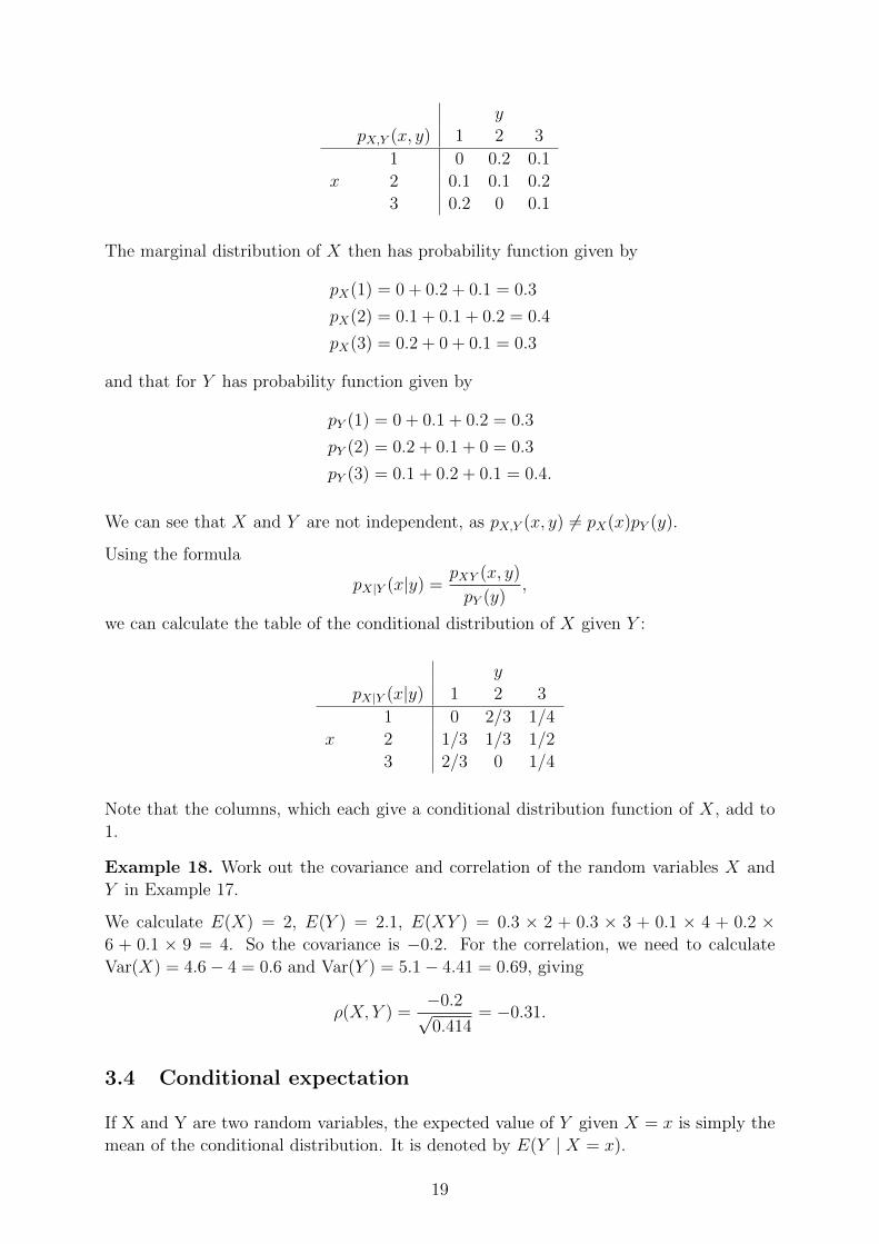
y

pX,Y (x, y) 1 2 3

1 0 0.2 0.1

x 2 0.1 0.1 0.2

3 0.2 0 0.1

The marginal distribution of X then has probability function given by

pX(1) = 0 + 0.2 + 0.1 = 0.3

pX(2) = 0.1 + 0.1 + 0.2 = 0.4

pX(3) = 0.2 + 0 + 0.1 = 0.3

and that for Y has probability function given by

pY (1) = 0 + 0.1 + 0.2 = 0.3

pY (2) = 0.2 + 0.1 + 0 = 0.3

pY (3) = 0.1 + 0.2 + 0.1 = 0.4.

We can see that X and Y are not independent, as pX,Y (x, y) 6= pX(x)pY (y).

Using the formula

pX|Y (x|y) =pXY (x, y)

pY (y),

we can calculate the table of the conditional distribution of X given Y :

y

pX|Y (x|y) 1 2 3

1 0 2/3 1/4

x 2 1/3 1/3 1/2

3 2/3 0 1/4

Note that the columns, which each give a conditional distribution function of X, add to

1.

Example 18. Work out the covariance and correlation of the random variables X and

Y in Example 17.

We calculate E(X) = 2, E(Y ) = 2.1, E(XY ) = 0.3 × 2 + 0.3 × 3 + 0.1 × 4 + 0.2 ×6 + 0.1 × 9 = 4. So the covariance is −0.2. For the correlation, we need to calculate

Var(X) = 4.6− 4 = 0.6 and Var(Y ) = 5.1− 4.41 = 0.69, giving

ρ(X, Y ) =−0.2√0.414

= −0.31.

3.4 Conditional expectation

If X and Y are two random variables, the expected value of Y given X = x is simply the

mean of the conditional distribution. It is denoted by E(Y | X = x).

19

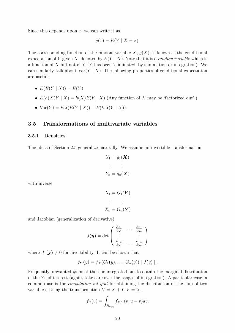
Since this depends upon x, we can write it as

g(x) = E(Y | X = x).

The corresponding function of the random variable X, g(X), is known as the conditional

expectation of Y given X, denoted by E(Y | X). Note that it is a random variable which is

a function of X but not of Y (Y has been ‘eliminated’ by summation or integration). We

can similarly talk about Var(Y | X). The following properties of conditional expectation

are useful:

• E(E(Y | X)) = E(Y )

• E(h(X)Y | X) = h(X)E(Y | X) (Any function of X may be ‘factorized out’.)

• Var(Y ) = Var(E(Y | X)) + E(Var(Y | X)).

3.5 Transformations of multivariate variables

3.5.1 Densities

The ideas of Section 2.5 generalize naturally. We assume an invertible transformation

Y1 = g1(X)

......

Yn = gn(X)

with inverse

X1 = G1(Y )

......

Xn = Gn(Y )

and Jacobian (generalization of derivative)

J(y) = det

∂x1∂y1

. . . ∂x1∂yn

......

∂xn∂y1

. . . ∂xn∂yn

where J (y) 6= 0 for invertibility. It can be shown that

fY (y) = fX(G1(y), . . . , Gn(y)) | J(y) | .

Frequently, unwanted ys must then be integrated out to obtain the marginal distribution

of the Y s of interest (again, take care over the ranges of integration). A particular case in

common use is the convolution integral for obtaining the distribution of the sum of two

variables. Using the transformation U = X + Y, V = X,

fU(u) =

∫RV |u

fX,Y (v, u− v)dv.

20

3.5.2 Approximate means and covariances

Now suppose that the random vector X has length n, mean µ and covariance matrix Σ,

see §3.2.2. Consider Y , a k-vector, obtained from X by application of the function g.

Thus Y = g(X) or, more explicitly,

Y1 = g1(X)

......

Yk = gk(X).

Note that, unlike in §3.5.1, k may be smaller than n. The idea is to get an approximation

for the mean vector and covariance matrix of Y . The approach show in §2.5.2 works here

too, but needs the multivariable version of Taylor’s theorem:

Y = g(X) ≈ g(µ) + g′(µ)(X − µ)

where g′(x) is the k × n matrix ∂g1∂x1

. . . ∂g1∂xn

......

∂gk∂x1

. . . ∂gk∂xn

.

Then, taking expectations, EY ≈ g(µ) and applying (2),

Cov(Y ) ≈ g′(µ)Σg′(µ)T ,

which does indeed give a k × k matrix, as it should.

This may seem rather abstract, but it is a powerful result when you have an estimated

covariance matrix for a set of quantities (coming out of your statistical analysis) and you

want to say something about the covariances of some function of them.

3.6 Standard multivariate distributions

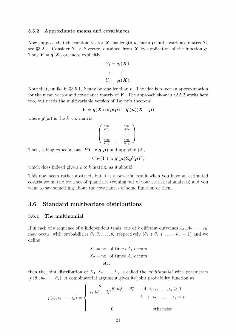
3.6.1 The multinomial

If in each of a sequence of n independent trials, one of k different outcomes A1, A2, . . . , Akmay occur, with probabilities θ1, θ2, . . . , θk respectively (θ1 + θ2 + . . . + θk = 1) and we

define

X1 = no. of times A1 occurs

X2 = no. of times A2 occurs

etc.

then the joint distribution of X1, X2, . . . , Xk is called the multinomial with parameters

(n; θ1, θ2, . . . , θk). A combinatorial argument gives its joint probability function as

p(i1, i2, . . . , ik) =

n!

i1!i2! . . . ik!θi11 θ

i22 . . . θ

ikk if i1, i2, . . . , ik ≥ 0

i1 + i2 + . . .+ ik = n

0 otherwise

21

The marginal distribution ofXr isBi(n, θr) and the distribution ofXr+Xs isBi(n, θr+θs),

which leads to the following results:

E(X)r = nθr

Var(Xr) = nθr(1− θr)Cov(Xr, Xs) = −nθrθs if r 6= s.

The likelihood function (see §4.5) is given by

L(θ;X) =n!

X1!X2! . . . Xk!θX1

1 θX22 . . . θXk

k

(assuming X1 +X2 + . . .+Xk = n) and the maximum likelihood estimators are θr = Xr

n

for r = 1, 2, . . . , k which are unbiased2.

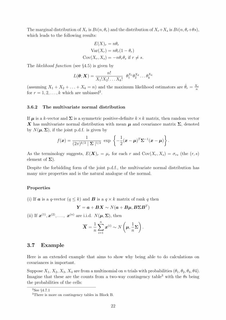
3.6.2 The multivariate normal distribution

If µ is a k-vector and Σ is a symmetric positive-definite k×k matrix, then random vector

X has multivariate normal distribution with mean µ and covariance matrix Σ, denoted

by N(µ,Σ), if the joint p.d.f. is given by

f(x) =1

(2π)k/2 | Σ |1/2exp

−1

2(x− µ)TΣ−1(x− µ)

.

As the terminology suggests, E(X)r = µr for each r and Cov(Xr, Xs) = σrs (the (r, s)

element of Σ).

Despite the forbidding form of the joint p.d.f., the multivariate normal distribution has

many nice properties and is the natural analogue of the normal.

Properties

(i) If a is a q-vector (q ≤ k) and B is a q × k matrix of rank q then

Y = a+BX ∼ N(a+Bµ,BΣBT )

(ii) If x(1),x(2), . . . , x(n) are i.i.d. N(µ,Σ), then

X =1

n

n∑i=1

x(i) ∼ N

(µ,

1

nΣ

).

3.7 Example

Here is an extended example that aims to show why being able to do calculations on

covariances is important.

SupposeX1, X2, X3, X4 are from a multinomial on n trials with probabilities (θ1, θ2, θ3, θ4).

Imagine that these are the counts from a two-way contingency table3 with the θs being

the probabilities of the cells:

2See §4.7.13There is more on contingency tables in Block B.

22

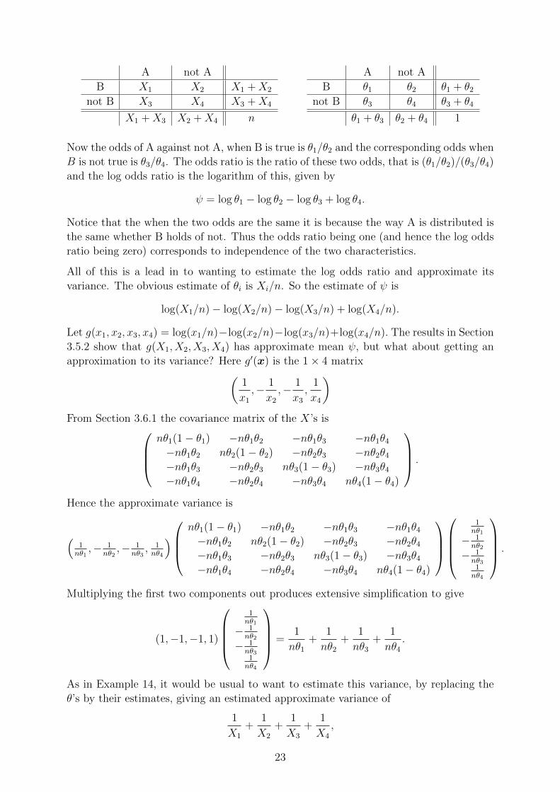
A not A

B X1 X2 X1 +X2

not B X3 X4 X3 +X4

X1 +X3 X2 +X4 n

A not A

B θ1 θ2 θ1 + θ2

not B θ3 θ4 θ3 + θ4

θ1 + θ3 θ2 + θ4 1

Now the odds of A against not A, when B is true is θ1/θ2 and the corresponding odds when

B is not true is θ3/θ4. The odds ratio is the ratio of these two odds, that is (θ1/θ2)/(θ3/θ4)

and the log odds ratio is the logarithm of this, given by

ψ = log θ1 − log θ2 − log θ3 + log θ4.

Notice that the when the two odds are the same it is because the way A is distributed is

the same whether B holds of not. Thus the odds ratio being one (and hence the log odds

ratio being zero) corresponds to independence of the two characteristics.

All of this is a lead in to wanting to estimate the log odds ratio and approximate its

variance. The obvious estimate of θi is Xi/n. So the estimate of ψ is

log(X1/n)− log(X2/n)− log(X3/n) + log(X4/n).

Let g(x1, x2, x3, x4) = log(x1/n)−log(x2/n)−log(x3/n)+log(x4/n). The results in Section

3.5.2 show that g(X1, X2, X3, X4) has approximate mean ψ, but what about getting an

approximation to its variance? Here g′(x) is the 1× 4 matrix(1

x1

,− 1

x2

,− 1

x3

,1

x4

)From Section 3.6.1 the covariance matrix of the X’s is

nθ1(1− θ1) −nθ1θ2 −nθ1θ3 −nθ1θ4

−nθ1θ2 nθ2(1− θ2) −nθ2θ3 −nθ2θ4

−nθ1θ3 −nθ2θ3 nθ3(1− θ3) −nθ3θ4

−nθ1θ4 −nθ2θ4 −nθ3θ4 nθ4(1− θ4)

.

Hence the approximate variance is

(1nθ1,− 1

nθ2,− 1

nθ3, 1nθ4

)nθ1(1− θ1) −nθ1θ2 −nθ1θ3 −nθ1θ4

−nθ1θ2 nθ2(1− θ2) −nθ2θ3 −nθ2θ4

−nθ1θ3 −nθ2θ3 nθ3(1− θ3) −nθ3θ4

−nθ1θ4 −nθ2θ4 −nθ3θ4 nθ4(1− θ4)

1nθ1

− 1nθ2

− 1nθ31nθ4

.

Multiplying the first two components out produces extensive simplification to give

(1,−1,−1, 1)

1nθ1

− 1nθ2

− 1nθ31nθ4

=1

nθ1

+1

nθ2

+1

nθ3

+1

nθ4

.

As in Example 14, it would be usual to want to estimate this variance, by replacing the

θ’s by their estimates, giving an estimated approximate variance of

1

X1

+1

X2

+1

X3

+1

X4

,

23

which is a nice memorable form. With a little bit more work we could show that the

same result is true if our original table had been r × s, instead of 2 × 2 and we had the

intersections of any picked any two rows and columns to identify the θ’s we were interested

in.

4 Introduction to inference and likelihood

4.1 Introduction

In probability theory we use the axioms of probability and their consequences as ‘rules

of the game’ for deducing what is likely to happen when an ‘experiment’ is performed.

In statistical inference we observe the outcome of an ‘experiment’ — which we call the

data — and use this as evidence to infer by what mechanism the observation has been

generated. Because of the apparent random variation in the data we assume that this

mechanism is a probability model; the data help us to reach some decision about the

nature of this model. Often in order to make the problem of inference tractable, we make

some broad assumptions about the form of the underlying probability model; the data

then help to narrow our choices within these assumptions.

As a common example, a collection of data of the same type, x1, x2, ..., xn say, may be

regarded as an observation on a sequence of independent identically distributed (i.i.d.)

random variables, X1, X2, ..., Xn say, whose common distribution is of some standard

form, e.g. normal or Poisson, but whose parameters are unknown. Such data constitute

a random sample. The data then give us information about the likely values of the

parameters.

These notes concentrate on classical (or frequentist) inference in which we assume that

the values of our underlying parameters are unknown, but fixed. An alternative approach

is Bayesian inference (see MAS6004) in which we express our initial uncertainty about

the true values of parameters by assigning them probability distributions. The data

then combine with these prior ideas to offer an updated distributional assessment of the

parameter values.

4.2 Types of (classical) inference

Three common types of inference are as follows

Point estimation A single number (which is a function of the observed data) is given

as an estimate of some parameter. The formula specifying the function is called an

estimator.

Interval estimation Instead of a single number, we specify a range (usually an interval)

of values in which the parameter is thought to lie on the basis of the observed data.

Testing hypotheses A hypothesis about a parameter value, or more generally about

the underlying probability model, is to be accepted or rejected on the basis of the

observed data.

24

Many other types of action are possible, e.g. ‘collect more data’.

4.3 Sampling distributions

Inference about a population is usually conducted in terms of a statistic t = T (x1, x2, ..., xn)

which is a function of the observed data. Regarded as a function of the corresponding

random variables, T = T (X1, X2, ..., Xn), this statistic is itself a random variable. Its

distribution is known as the sampling distribution of the statistic. In principle this distri-

bution can be derived from the distribution of the data; in practice this may or may not

be possible. The sampling distribution is important because it enables us to construct

good inferential procedures and to quantify their effectiveness.

Example 19. If X1, X2, ..., Xn is a random sample from the normal distribution N(µ, σ2)

then two important statistics are the sample mean

X =1

n

n∑i=1

Xi

and the sample variance

S2 =1

n− 1

n∑i=1

(Xi −X)2

which are used to estimate µ and σ2 respectively. It may be shown that

X ∼ N

(µ,σ2

n

),

(n− 1)S2

σ2∼ χ2

n−1

and that X and S2 are independent.

The first result above, for instance, tells us how precise X is as an estimator of µ: it has

‘mean square error’

E(X − µ

)2= Var(X) =

σ2

n

which decreases as the sample size n increases.

4.4 Normal approximations for large samples

In the preceding example, we note that if the probability model is correct (i.e. if X1, X2,

. . . , Xn are i.i.d. random variables each with N(µ, σ2) distribution) then the sampling

distribution of X is known exactly. But the central limit theorem tells us that even

if the distribution of the Xs is not normal in form, the sampling distribution of X is

approximately normal in form if the sample size n is large. We say that the sampling

distribution of X is asymptotically normal.

The important consequence of this result is that we can conduct inference using the

sampling distribution of X without being too concerned what the underlying distribution

of the Xs is.

25

There are many other statistical models in which the sampling distribution of a statistic

is asymptotically normal ; in other cases it may be e.g. asymptotically χ2 (which typi-

cally has behind it a result about some multivariate statistic being multivariate normal

by the central limit theorem). The beauty of these results is that what might be an in-

tractable distributional problem is made tractable by an approximation using a standard

distribution. Such methods are known as large sample methods.

4.5 Likelihood

A key tool in many classical and Bayesian approaches to inference is the likelihood function.

We often have some reason (for example a probabilistic model for the process producing

the data) to assume a particular form for the joint p.d.f. of X, usually involving some

standard distribution. However, the parameters of the standard distribution will usually

be unknown, and our aim in analysing the data will be to obtain information about the

values of these unknown parameters.

General parameters are usually denoted by θ; we represent θ as a vector, although in any

particular case the set of parameters can be a scalar (a single number), a matrix or some

other structure.

If we have a statistical model with parameter values θ then f(x|θ) is a p.d.f. (in the

continuous case) and as such it defines the distribution of X, given values of θ.

(If we have discrete random variables, then we would have a probability function instead

of a p.d.f. The theory in this case is very similar, so it is common to use the same notation

in both cases.)

Once we have observed data values x (a realisation of X) we can consider f(x|θ) as a

function of θ. Note that, considered this way, it is no longer a p.d.f.; in particular there

is no requirement for it to integrate to 1.

Definition:

When we regard f(x|θ) as a function of θ, for the fixed (observed) data x, it is called

the likelihood function (or just the likelihood). We will denote it by L(θ;x) and we say

that L(θ;x) is the likelihood of θ based on data x.

The likelihood is a function of the parameter θ. Thus, to describe completely the like-

lihood, it is important, when we calculate L(θ;x), to identify the set of the possible

parameter values θ, that is the domain of L. We will denote the set of possible parameter

values by Θ.

In a situation in which X1, . . . , Xn are not a random sample (so they are not i.i.d.), the

likelihood is still just the joint p.d.f. or probability function of the variables, but this will

no longer be a simple product of terms of identical form.

This function provides the basic link between the data and unknown parameters so it is

not surprising that it is used throughout classical inference in determining (theoretically

or graphically) estimates, test statistics, confidence intervals and their properties and

underpins the entire Bayesian approach. In many situations it is more natural to consider

26

the natural logarithm (but we usually use log for this rather than ln) of the likelihood

function

`(θ;x) = log(L(θ;x)).

This is often denoted simply l(θ).

4.6 Maximum likelihood estimation

If we approach inference from a likelihood-based perspective, then a natural choice of

point estimator for θ is the maximum likelihood estimator θ = θ(X1, X2, . . . , Xn) where

θ is such that

L(θ;X) = maxθ

L(θ;X)

This is the value which gives the observed data the highest likelihood (i.e., in the discrete

case, the highest probability of having occurred).

Example 20. Let x1, x2, ..., xn be a random sample from Po(µ).

L(µ;x) = e−µµx1

x1!. . . e−µ

µxn

xn!.

It is easier to maximize

`(µ) = logL(µ;x) = −nµ+

(n∑i=1

xi

)log µ−

n∑i=1

log xi!.

Differentiating,d`

dµ= −n+

∑xiµ

= 0 when µ =

∑xin

= x.

Therefore µ = µ(X1, X2, . . . , Xn) = X is the maximum likelihood estimator of µ. You can

check that the second derivative is negative to confirm that this is indeed a maximum.

Example 21. Let x1, x2 . . . , xn be the values of independent observations of exponential

random variables with unknown parameter µ (mean 1/µ). Then the likelihood function

is

L(x|µ) =n∏j=1

µe−µxj = µnn∏j=1

e−µxj

and the log likelihood l(x|µ) = n log µ− µ∑n

j=1 xj.

To find the maximum likelihood estimate, differentiate l(x|µ) with respect to µ:

dl(x|µ)

dµ=n

µ−

n∑j=1

xj.

So at a maximum we will haven

µ=

n∑j=1

xj,

27

which implies that at a maximum µ = n/∑n

j=1 xj = 1/x. To check that this really is a

maximum, look at the second derivative:

d2l(x|µ)

dµ2= − n

µ2,

which is negative, indicating that we have indeed found a maximum.

So the maximum likelihood estimate is µ = 1/x. (Note that we write µ to distinguish

this from the true value of the parameter µ, which was what we were trying to estimate,

but the actual value of which remains unknown.)

Notes: 1) It is equivalent and often easier to maximize the natural logarithm of the

likelihood rather than L itself. 2) Writing the process in terms of the observed likelihood

L(θ;x) leads to the maximum likelihood estimate rather than the maximum likelihood

estimator. (The first is a function of the actual values, x, the second of the random

variablesX.) This may tempt you into notational inaccuracy when considering properties

of m.l.e.s, etc.

4.7 Properties of estimators

4.7.1 Unbiasedness

If τ(θ) is some function of a parameter θ and T (X1, ..., Xn) = T (X) is some function of

X, then T is an unbiased estimator of τ if

Eθ[T (X)] = τ(θ)

for all values of θ. [Eθ denotes expected value with respect to the sampling distribution

of T when θ is the true value of the parameter]. In other words, ‘on average’ T gives the

right answer.

Example 22. If X1, X2, ..., Xn is a random sample from any distribution with mean µ

and

X =X1 +X2 + ...+Xn

n,

then EX = µ as we have seen earlier. Hence X is an unbiased estimator of µ.

Unbiasedness is a desirable property in general, but not always, as the following example

shows.

Example 23. Let X be an observation from Po(µ), and suppose we wish to estimate

τ(µ) = e−2µ. If we define

T (X) =

1 if X is even

−1 if X is odd

then

E[T (X)] =∞∑i=0

(−1)ie−µµi

i!= e−µ.e−µ = e−2µ

and so T is an unbiased estimator of e−2µ. But is is an absurd estimator, because e.g.

e−2µ cannot take the value −1.

28

4.7.2 Mean square error and efficiency

If T (X) is an estimator of τ(θ), then its mean square error (m.s.e.) is given by

Eθ[T (X)− τ(θ)]2

In particular, if T (X) is unbiased for τ(θ), then the above is the same as the variance of

T (X). It is a measure of the likely accuracy of T as an estimator of t: the larger it is,

the less accurate the estimator.

If T and T ′ are two different estimators of t, the relative efficiency of T ′ is given by the

ratioEθ(T − τ)2

Eθ(T ′ − τ)2

This appears to depend on θ, but in many cases it does not.

Example 24. Let X1, X2, ..., X2m+1 be a random sample (of odd size) from N(µ, σ2), let

X be the sample mean, and let M be the sample median, i.e. the (m+ 1)th data value in

ascending order. X and M are both unbiased estimators of µ; we know that

Var(X) =σ2

2m+ 1,

and it may be shown that

Var(M) =πσ2

2(2m+ 1)

for large m. Hence the (asymptotic) relative efficiency of M with respect to X as an

estimator of µ isσ2

2m+ 1· 2(2m+ 1)

πσ2=

2

π.

M is less efficient than X by this factor.

5 Interval estimation and hypothesis testing

5.1 Interval estimation

In point estimation we aim to produce a single ‘best guess’ at a parameter value θ. Here,

in contrast, we provide a region (usually an interval) in which θ ‘probably lies’.

Construction is via inversion of a probability statement concerning the data, so if T is a

statistic derived from the data we find, by examining the sampling distribution of T , a

region A(θ) such that

P (T ∈ A(θ)) = 1− α (4)

for some suitable small α, and invert this to identify the region C(T ) = [θ : T ∈ A(θ)]

which then satisfies

P (θ ∈ C(T )) = 1− α. (5)

29

In other words, the ‘random region’ C(T ) ‘covers’ the true parameter value θ with prob-

ability 1− α. In simple situations C(T ) is an interval, called a confidence interval for θ.

The confidence level is usually expressed as a percentage: 100(1-α)% (e.g. α = 0.05 gives

a 95% confidence interval).

Example 25. X1, X2, ..., Xn a random sample from N(µ, σ2) with µ unknown, σ2 known.

T = X with

X ∼ N(µ, σ2/n).

ThusX − µσ/√n∼ N(0, 1)

P

(−z1−α/2 ≤

X − µσ/√n≤ z1−α/2

)= 1− α (6)

where z1−α/2 solves Φ(z1−α/2) = 1− α/2 (from tables).

Thus

P

(µ− z1−α/2

σ√n≤ X ≤ µ+ z1−α/2

σ√n

)= 1− α (7)

so

A(µ) =

(µ− z1−α/2

σ√n, µ+ z1−α/2

σ√n

)Inverting (7)

P

[X − z1−α/2

σ√n≤ µ ≤ X + z1−α/2

σ√n

]= 1− α

i.e.

C(T ) =

(X − z1−α/2

σ√n,X + z1−α/2

σ√n

).

Note: we have chosen the z1−α/2 in (6) symmetrically; we could have chosen any z values

giving overall probability level 1− α.

In general if an estimator θ is asymptotically normally distributed with mean equal to

the true value of the parameter θ, then an approximate 100(1− α)% confidence interval

is given by (θ − z1−α/2σθ, θ + z1−α/2σθ

)where σθ, the standard deviation of the sampling distribution of θ, is called the standard

error. This may itself have to be estimated from the data.

5.2 Introduction to testing hypotheses

A hypothesis is a statement about the underlying probability model which may or may not

be true. We do not know which. We can, however, obtain some information by looking

at the data. A test is a decision rule which attaches a verdict (‘do not reject’ or ‘reject’)

to each possible set of observed data. Ideally we would like to make the right decision

most of the time.

30

If the model is specified up to an unknown (vector) parameter θ say, then a hypothesis

H is a statement restricting θ to some subset Θ0 of the parameter space Θ. If H specifies

completely the distribution of the data, it is called a simple hypothesis (usually this means

Θ0 is a singleton); otherwise it is composite. A null hypothesis (typically denoted H0) is

one of particular interest — typically the default/status quo/no effect hypothesis.

5.3 Pure significance tests (for simple H0)

In addition to our null hypothesis H0 we need some idea of the type of departures from

H0 which are of interest.

Example 26. Data X1, X2, ..., Xn; H0 : Xi ∼ N(0, 1) i.i.d.

Possible departures of interest:

(a) increase in mean,

(b) increase in variance,

(c) correlation between successive individuals.

To formulate a pure significance test we need to find a statistic T (X) such that

(i) the values of T increase with departure from H0 in the direction of interest;

(ii) the distribution of T is known when H0 is assumed true.

For the departures from H0 in Example 26 we might use the following test statistics:

(a) Use X ∼ N(0, 1/n) on H0 (note terminology).

(b) Use∑n

i=1X2i ∼ χ2

n on H0.

(c) Use∑n−1

1 XiXi+1 distribution known on H0

We evaluate tobs, the observed value of T , and find pobs = P (T ≥ tobs | H0 true) — the

p-value or observed (or exact) significance level of T. This is the probability, under H0,

of getting a value of T at least as extreme as the one observed.

In specifying the result of the test we would either quote the p-value directly, or, if p ≤ α

for some small preassigned value α, say ‘the data depart significantly (at level α) from

H0 (in the direction of interest)’.

5.4 Hypothesis tests

Here we specify formally both our null hypothesis H0 : θ ∈ Θ0 and an alternative hypoth-

esis H1 : θ ∈ Θ1 (often Θc0) representing our ‘departures of interest’.

Any test divides the set of possible data sets X say, into an non-rejection region X0 and

a critical region X1 such that if the observed x lies in X1 we reject H0 and otherwise we

do not reject it.

31

In principle we can evaluate, for each θ ∈ Θ, the probability thatX lies in X1; the function

γ(θ) = Pθ(X ∈ X1)

is called the power function of the test and summarises its properties. Ideally we wish to

choose X1 so that γ(θ) is small (close to 0) for θ ∈ Θ0 and large (close to 1) when θ ∈ Θ1.

The number

α = supθ∈Θ0

γ(θ)

is called the size of the test, this is the maximum probability of rejecting H0 if it is true.

Often, instead X, we work in terms of a statistic T = T (X), say, known as the test

statistic; it is then convenient to define the non-rejection and critical regions in terms of

T rather than X.

5.5 Constructing tests

5.5.1 Intuition

Often the form of a test (i.e. the form of the critical region) will be suggested by intuition.

For example, if T is a good estimator of a parameter θ and the hypotheses take the

‘one-sided’ form

H0 : θ ≤ θ0 H1 : θ > θ0

for some fixed given θ0, then we would expect that the larger the value of T , the greater

the evidence in favour of H1; and so a sensible critical region will be of the form T > cfor some constant c. Then

γ(θ) = Pθ(T > c).

To choose c: as c increases, γ(θ) decreases for all values of θ; for θ ∈ Θ0 this is a good

thing, whereas for θ ∈ Θ1 it is a bad thing. So we must choose c so as to strike a balance.

Often this is done by prescribing the value of α (e.g. 0.05). This is sufficient to determine

c. Often tables of critical values of the test statistic for specified α are produced.

Example 27. X1, X2, ..., Xn a sample from N(µ, 1).

H0 : µ ≤ 0 H1 : µ > 0.

Use X as test statistic; critical region will be of the form x > c.

γ(µ) = Pµ(X > c) = 1− Φ

(c− µ1/√n

)= Φ

(√n(µ− c)

).

This has its maximum value in H0 when µ = 0; so if α is prescribed we must choose c

such that Φ(−c√n) = α. This is easily solved for c (using tables).

If n = 100, α = 0.05 Φ(−10c) = 0.05 c = −110

Φ−1(0.05) Neave table 2.3(b) gives c =−110

(−1.6449) = 0.16449. So the test is ‘reject H0 : µ ≤ 0 at the 5% level if x > 0.16449’

32

5.5.2 Neyman-Pearson approach

This form is most easily introduced in the (not very practically useful) case of choosing

between two simple hypotheses H0 : θ = θ0 versus H1 : θ = θ1 (it can be extended to

composite hypotheses).

We consider the probabilities of making the two types of error that can occur in any test

α = P (type I error) = P (reject H0 | H0 true) = γ(θ0) as before;

β = P (type II error) = P (do not reject H0 | H1 true) = 1− γ(θ1).

Again, ideally we would like both α and β small, but simultaneous reduction is usually

impossible so we compromise by fixing α at an acceptably low level and then minimising

β (for this fixed α).

The Neyman-Pearson lemma tells us that the test with

X1 =

x :

L(θ0;x)

L(θ1;x)< c

where c is such that P (X ∈ X1 | θ0) = α will minimize β = P (X ∈ X0 | θ1), i.e. it is the

most powerful test of level α.

Typically the form of the test simplifies and we can work with a particular test statistic

T and determine probabilities from its sampling distribution.

Example 28. X1, X2, ..., Xn a sample from N(µ, σ2), σ2 known.

H0 : µ = µ0 H1 : µ = µ1 with µ1 > µ0 say.

Intuition suggests a test with critical region X > c and this is indeed the most powerful

test:

L(µ;X) =1

(2π)n/2(σ2)n/2exp

−1

2

n∑i=1

(Xi − µ)2

σ2

.

So the N-P lemma says the best test has critical region given by X’s for which

exp

− 1

2σ2

[∑(Xi − µ0)2 −

∑(Xi − µ1)2

]< c

i.e. − 1

2σ2

[∑X2i − 2µ0

∑Xi + µ2

0 −∑

X2i + 2µ1

∑Xi − µ2

1

]< c′

i.e.∑Xi(µ1 − µ0) > c′′ (take care over direction of inequality)

i.e. X > c′′′ = k say recalling µ1 − µ0 > 0.

Now k is determined by the requirement

P (X ∈ X1 | µ = µ0) = α i.e. P (X > k | µ = µ0) = α.

The sampling distribution of X is N(µ0, σ2/n) when H0 holds. Therefore

P (X > k | µ = µ0) = P

(X − µ0

σ/√n>k − µ0

σ/√n

)= α.

i.e. k = µ0 + σ√nΦ−1(1− α) evaluated using Neave 2.3(b).

33

5.5.3 The likelihood ratio procedure

This is a method of suggesting a form of test which in principle always works. It gives

the same result as the Neyman-Pearson test in the simple versus simple case (despite the

difference in the denominator) and extends easily to more general situations. There is

also a useful asymptotic result about it (see later). The test is defined by considering the

ratiosupθ∈Θ0

L(θ;x)

supθ∈Θ

L(θ;x)= Λ.

This ratio is always < 1 since the supremum in the denominator is over a larger set. The

further Λ is from 1, the greater the evidence against H0. Hence a form of critical region

which suggests itself is Λ < c.

Example 29. X1, X2, ..., Xn a sample from N(µ, σ2) with both µ and σ2 unknown.

H0 : µ = µ0 H1 : µ 6= µ0 (a ‘two-sided’ alternative).

Here Θ0 = (µ, σ2); µ = µ0, σ2 > 0 and Θ = (µ, σ2); σ2 > 0.

The likelihood is

L(θ;X) =1

(2π)n/2(σ2)n/2exp

[−1

2

n∑i=1

(Xi − µ)2

σ2

].

This is maximized in Θ0 by putting µ = µ0 and σ2 = 1n

∑ni=1(Xi − µ0)2 (check by

differentiating!), giving

maxθ∈Θ0

L(θ;X) =nn/2 e−n/2

(2π)n/2 [∑

(Xi − µ0)2]n/2,

It is maximized in Θ by putting µ = X and σ2 = 1n

∑ni=1(Xi −X)2, giving

maxθ∈Θ

L(θ;X) =nn/2 e−n/2

(2π)n/2[∑

(Xi −X)2]n/2 .

Hence the critical region takes the form (from the ratio of the previous two expressions)(∑(Xi −X)2∑(Xi − µ0)2

)n/2< c.

Since∑

(Xi − µ0)2 =∑

(Xi −X)2 + n(X − µ0)2, this is equivalent to

(X − µ0)2∑(Xi −X)2

> c′

orX − µ0

S> c′′

where S2 is the sample variance.

34

The statistic

T =

√n(X − µ0)

S

is called the one-sample t statistic. Its sampling distribution if µ = µ0 does not depend

upon σ2, and is known as the t distribution with n − 1 degrees of freedom. So a test of

given size may be constructed using tables of critical values for this distribution (Neave

3.1).

The form of test suggested by the likelihood ratio procedure often simplifies, as above,

but the sampling distribution of the simplified test statistic must be derived by ‘ad hoc’

methods — and this is not always possible. It is, therefore, useful to have a general

asymptotic result which works under reasonable regularity conditions as the sample size

n → ∞; this is that if H0 is true −2 log Λ is asymptotically χ2ν where ν, the number of

degrees of freedom, is the difference in dimensionality between Θ0 and Θ.

Example 30. (X11, ..., X1n), (X21, ..., X2n), . . . , (Xk1, ..., Xkn) are samples fromN(µ1, σ21),

. . . , N(µk, σ2k) respectively where µ1, σ

21, . . . , µk, σ

2k are all unknown, and we wish to test

H0 : σ21 = σ2

2 = . . . = σ2k. Then the unrestricted parameter space Θ is 2k-dimensional

whereas Θ0 is (k + 1)-dimensional, since H0 imposes (k − 1) linear constraints. Hence

−2 log Λ ∼ X2k−1 asymptotically.

5.6 Duality between interval estimation and hypothesis testing

There is a duality between interval estimation and hypothesis testing in that possible

parameter values which would not be rejected in a size α test are those which constitute

the 100(1− α)% confidence interval. This gives us a direct means of establishing A(θ) in

(4).

Let A(θ0) denote the acceptance region for a standard test of size α of H0 : θ = θ0 (simple)

against H1 : θ 6= θ0 using a test statistic T . Then we have

Pθ0(T ∈ A(θ0)) = 1− α for all θ0.

Defining C(T ) as in (5), this may be written

Pθ(θ ∈ C(T )) = 1− α.

So C(T ) is a confidence interval for θ.

35