Embed Size (px)
Citation preview
MS Office 2010
Excel Formulas
&
Functions Part 1 www.catraining.co.uk
Tel: 020 7920 9500

i
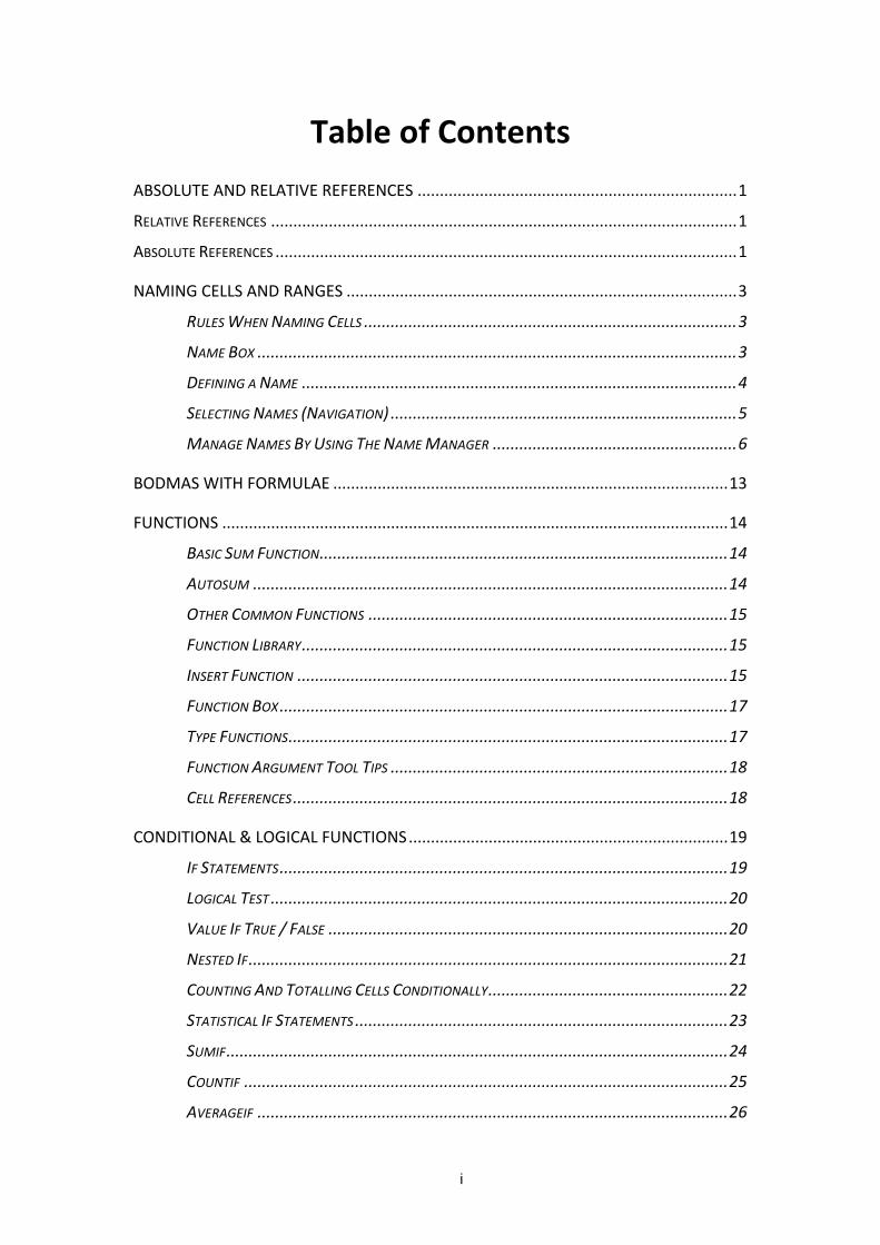
Table of Contents
ABSOLUTE AND RELATIVE REFERENCES ........................................................................ 1
RELATIVE REFERENCES ......................................................................................................... 1
ABSOLUTE REFERENCES ........................................................................................................ 1
NAMING CELLS AND RANGES ........................................................................................ 3
RULES WHEN NAMING CELLS .................................................................................... 3
NAME BOX ............................................................................................................ 3
DEFINING A NAME .................................................................................................. 4
SELECTING NAMES (NAVIGATION) .............................................................................. 5
MANAGE NAMES BY USING THE NAME MANAGER ....................................................... 6
BODMAS WITH FORMULAE ......................................................................................... 13
FUNCTIONS .................................................................................................................. 14
BASIC SUM FUNCTION ............................................................................................ 14
AUTOSUM ........................................................................................................... 14
OTHER COMMON FUNCTIONS ................................................................................. 15
FUNCTION LIBRARY ................................................................................................ 15
INSERT FUNCTION ................................................................................................. 15
FUNCTION BOX ..................................................................................................... 17
TYPE FUNCTIONS ................................................................................................... 17
FUNCTION ARGUMENT TOOL TIPS ............................................................................ 18
CELL REFERENCES .................................................................................................. 18
CONDITIONAL & LOGICAL FUNCTIONS ........................................................................ 19
IF STATEMENTS ..................................................................................................... 19
LOGICAL TEST ....................................................................................................... 20
VALUE IF TRUE / FALSE .......................................................................................... 20
NESTED IF ............................................................................................................ 21
COUNTING AND TOTALLING CELLS CONDITIONALLY ...................................................... 22
STATISTICAL IF STATEMENTS .................................................................................... 23
SUMIF ................................................................................................................. 24
COUNTIF ............................................................................................................. 25
AVERAGEIF .......................................................................................................... 26
ii
AVERAGEIFS ......................................................................................................... 27
SUMIFS ............................................................................................................... 28
COUNTIFS ............................................................................................................ 30
AND, OR, NOT ............................................................................................................... 31
AND FUNCTION .................................................................................................... 32
OR FUNCTION ...................................................................................................... 32
NOT FUNCTION ..................................................................................................... 33
ISERROR FUNCTION ............................................................................................. 33
IFERROR FUNCTION ............................................................................................. 34
LOOKUP FUNCTIONS .......................................................................................................... 36
LOOKUP .............................................................................................................. 36
VECTOR LOOKUP ................................................................................................... 36
HLOOKUP ............................................................................................................ 38
VLOOKUP ............................................................................................................ 40
NESTED LOOKUPS .................................................................................................. 41
MATCH() ........................................................................................................... 42
TWO-WAY LOOKUP ............................................................................................... 42
INDEX FUNCTION ................................................................................................. 43
COMBINING MATCH AND INDEX ........................................................................... 44
CHOOSE .............................................................................................................. 45
OFFSET ............................................................................................................... 46
FINANCIAL FUNCTIONS ................................................................................................ 48
NPV() ................................................................................................................ 48
COMPARING INVESTMENT SCHEDULES ....................................................................... 49
IRR() .................................................................................................................. 50
PMT() ................................................................................................................ 51
CALCULATING LOAN REPAYMENTS ............................................................................ 52
FV() ................................................................................................................... 52
DATE & TIME CALCULATIONS ...................................................................................... 54
DATES ................................................................................................................. 54
NETWORKDAYS() .............................................................................................. 54
ANALYSIS TOOLPAK ............................................................................................... 54
TODAY() ............................................................................................................ 55
iii
NOW ................................................................................................................. 56
DAY(), MONTH() AND YEAR()............................................................................ 56
TIME CALCULATIONS .......................................................................................................... 57
SUBTRACTING TIMES .............................................................................................. 57
TOTALLING TIMES ................................................................................................. 57
TEXT FUNCTIONS ......................................................................................................... 60
PROPER, UPPER, LOWER, REPT ........................................................................ 60
CONCATENATE ................................................................................................. 60
STRING FUNCTIONS (LEFT, MID, RIGHT) ................................................................................ 61
LEFT FUNCTION ................................................................................................... 61
MID FUNCTION .................................................................................................... 61
RIGHT FUNCTION ................................................................................................. 61

iv
Excel Formulas and Functions.docx Absolute And Relative References
Page 1
Absolute And Relative References
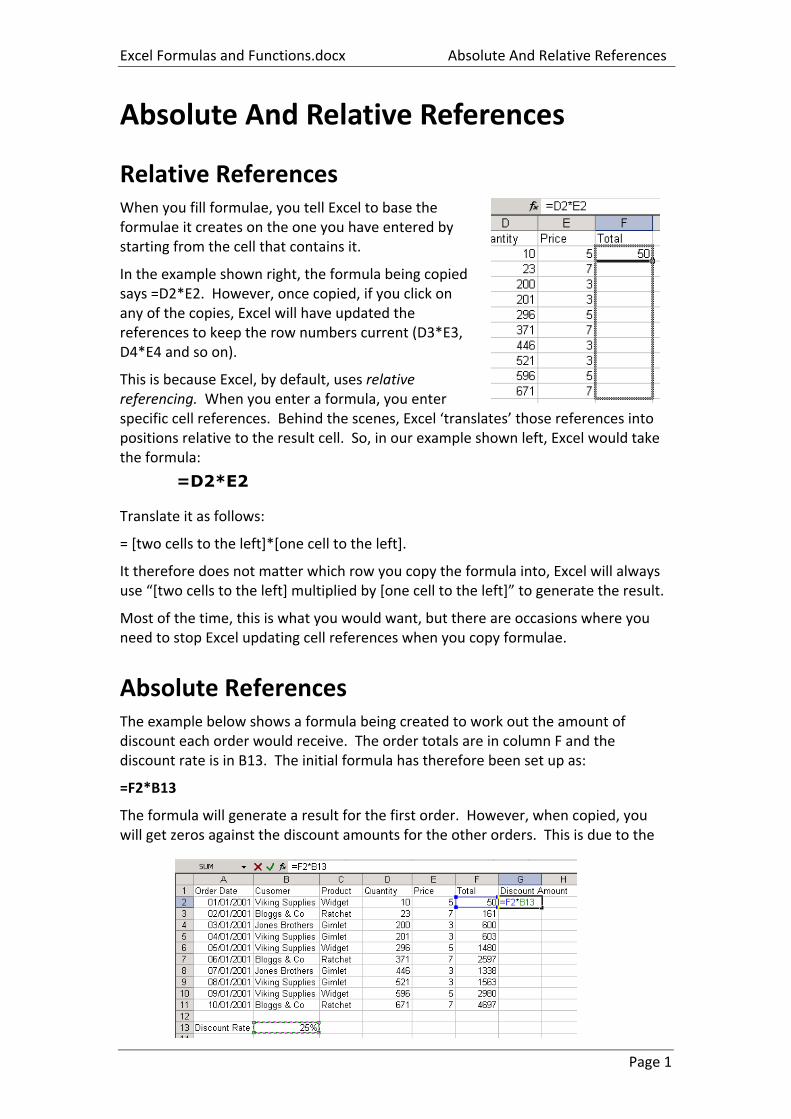
Relative References When you fill formulae, you tell Excel to base the formulae it creates on the one you have entered by starting from the cell that contains it.
In the example shown right, the formula being copied says =D2*E2. However, once copied, if you click on any of the copies, Excel will have updated the references to keep the row numbers current (D3*E3, D4*E4 and so on).
This is because Excel, by default, uses relative referencing. When you enter a formula, you enter specific cell references. Behind the scenes, Excel ‘translates’ those references into positions relative to the result cell. So, in our example shown left, Excel would take the formula:
=D2*E2
Translate it as follows:
= [two cells to the left]*[one cell to the left].
It therefore does not matter which row you copy the formula into, Excel will always use “[two cells to the left] multiplied by [one cell to the left]” to generate the result.
Most of the time, this is what you would want, but there are occasions where you need to stop Excel updating cell references when you copy formulae.
Absolute References The example below shows a formula being created to work out the amount of discount each order would receive. The order totals are in column F and the discount rate is in B13. The initial formula has therefore been set up as:
=F2*B13
The formula will generate a result for the first order. However, when copied, you will get zeros against the discount amounts for the other orders. This is due to the
Absolute And Relative References Excel Formulas and Functions.docx
Page 2
relative referencing that Excel applies to all formulae by default.
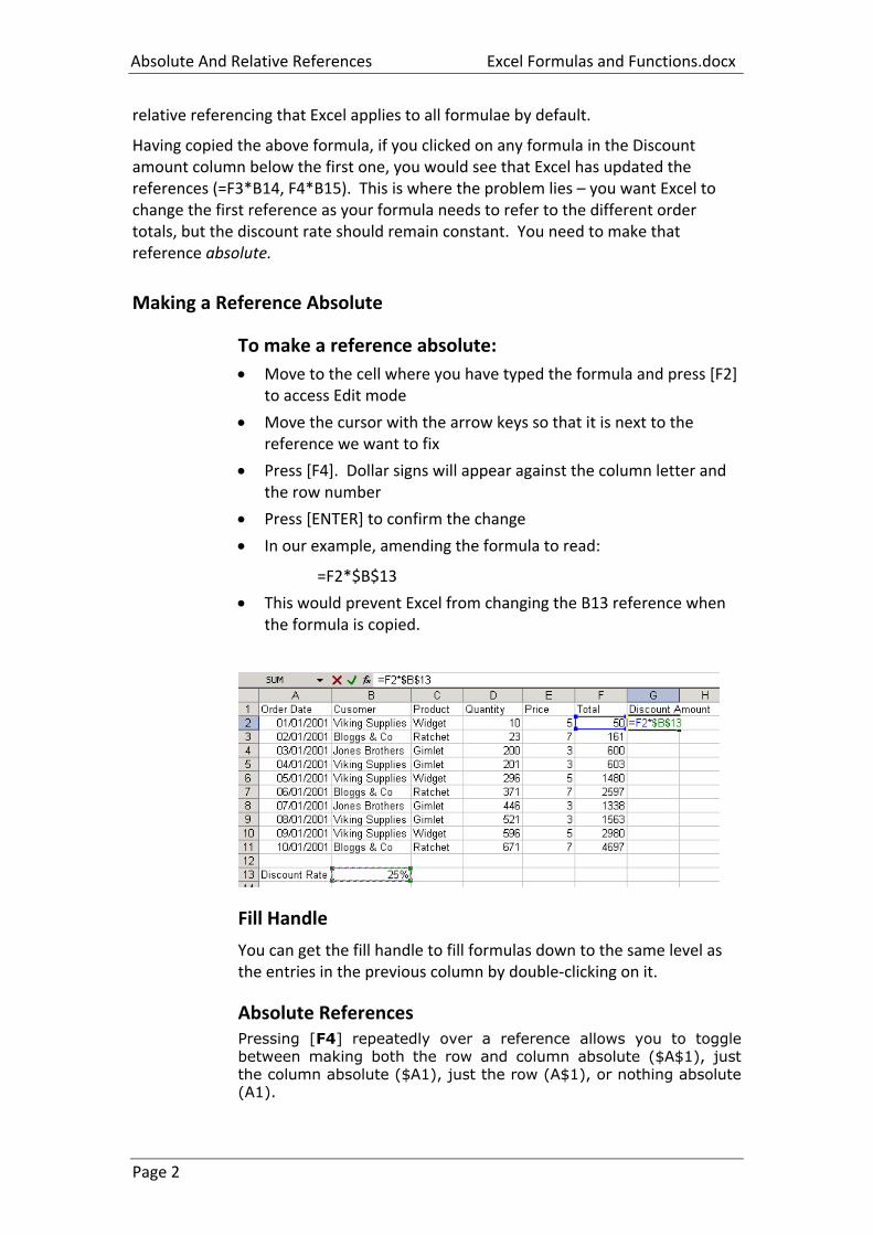
Having copied the above formula, if you clicked on any formula in the Discount amount column below the first one, you would see that Excel has updated the references (=F3*B14, F4*B15). This is where the problem lies – you want Excel to change the first reference as your formula needs to refer to the different order totals, but the discount rate should remain constant. You need to make that reference absolute.
Making a Reference Absolute
To make a reference absolute:
Move to the cell where you have typed the formula and press [F2] to access Edit mode
Move the cursor with the arrow keys so that it is next to the reference we want to fix
Press [F4]. Dollar signs will appear against the column letter and the row number
Press [ENTER] to confirm the change
In our example, amending the formula to read:
=F2*$B$13
This would prevent Excel from changing the B13 reference when the formula is copied.
Fill Handle
You can get the fill handle to fill formulas down to the same level as the entries in the previous column by double-clicking on it.
Absolute References Pressing [F4] repeatedly over a reference allows you to toggle
between making both the row and column absolute ($A$1), just
the column absolute ($A1), just the row (A$1), or nothing absolute (A1).
Excel Formulas and Functions.docx Naming Cells and Ranges
Page 3
Naming Cells and Ranges When entering formulae or referring to an area in a workbook, it is usual to refer to a ‘range’. For example, B6 is a range reference; B6:B10 is also a range reference. One problem with this sort of reference is that it is not very meaningful and therefore easily forgettable. If you want to refer to a range several times in formulae or functions, you may find it necessary to write it down, or select it, which often means wasting time scrolling around the workbook. Instead, Excel offers the chance to name ranges in a workbook, and to use these names to select cells, refer to them in formulae or use them in Database, Chart or Macro commands.
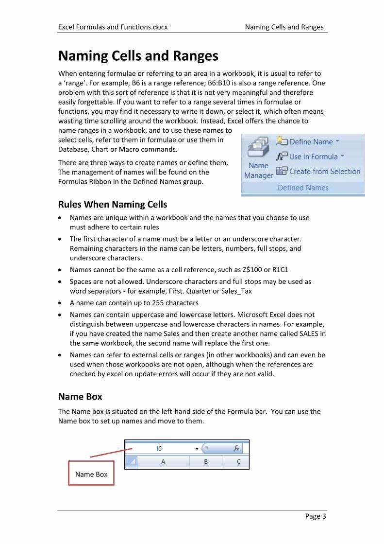
There are three ways to create names or define them. The management of names will be found on the Formulas Ribbon in the Defined Names group.
Rules When Naming Cells Names are unique within a workbook and the names that you choose to use
must adhere to certain rules
The first character of a name must be a letter or an underscore character. Remaining characters in the name can be letters, numbers, full stops, and underscore characters.
Names cannot be the same as a cell reference, such as Z$100 or R1C1
Spaces are not allowed. Underscore characters and full stops may be used as word separators - for example, First. Quarter or Sales_Tax
A name can contain up to 255 characters
Names can contain uppercase and lowercase letters. Microsoft Excel does not distinguish between uppercase and lowercase characters in names. For example, if you have created the name Sales and then create another name called SALES in the same workbook, the second name will replace the first one.
Names can refer to external cells or ranges (in other workbooks) and can even be used when those workbooks are not open, although when the references are checked by excel on update errors will occur if they are not valid.
Name Box
The Name box is situated on the left-hand side of the Formula bar. You can use the Name box to set up names and move to them.
Name Box
Absolute References Naming Cells and Ranges
Page 4
Defining a Name
To define a name
Select the cell or cells you wish to name
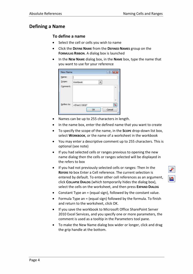
Click the DEFINE NAME from the DEFINED NAMES group on the FORMULAS RIBBON. A dialog box is launched
In the NEW NAME dialog box, in the NAME box, type the name that you want to use for your reference
Names can be up to 255 characters in length.
In the name box, enter the defined name that you want to create
To specify the scope of the name, in the SCOPE drop-down list box, select WORKBOOK, or the name of a worksheet in the workbook
You may enter a descriptive comment up to 255 characters. This is optional (see note)
If you had selected cells or ranges previous to opening the new name dialog then the cells or ranges selected will be displayed in the refers to box
If you had not previously selected cells or ranges: Then In the REFERS TO box Enter a Cell reference. The current selection is entered by default. To enter other cell references as an argument, click COLLAPSE DIALOG (which temporarily hides the dialog box), select the cells on the worksheet, and then press EXPAND DIALOG
Constant Type an = (equal sign), followed by the constant value.
Formula Type an = (equal sign) followed by the formula. To finish and return to the worksheet, click OK.
If you save the workbook to Microsoft Office SharePoint Server 2010 Excel Services, and you specify one or more parameters, the comment is used as a tooltip in the Parameters tool pane.
To make the New Name dialog box wider or longer, click and drag the grip handle at the bottom.
Excel Formulas and Functions.docx Naming Cells and Ranges
Page 5
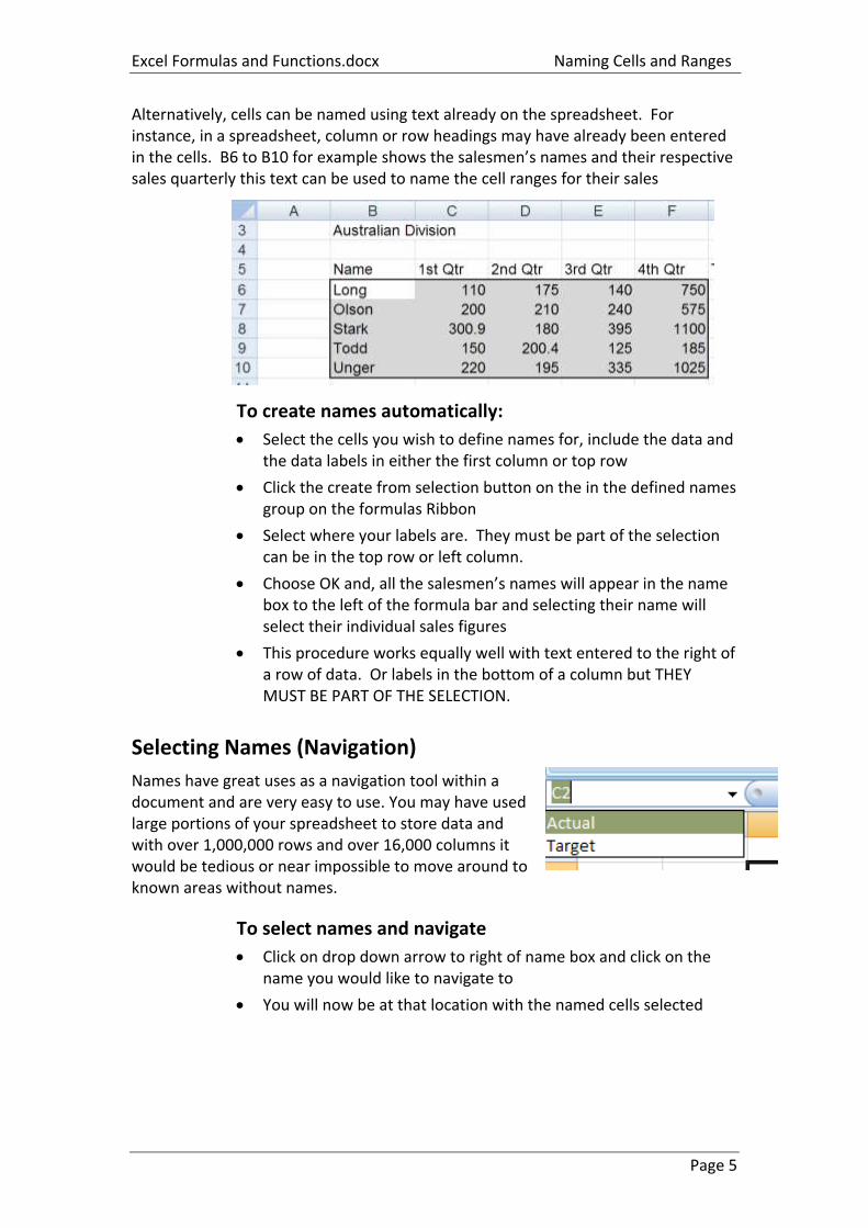
Alternatively, cells can be named using text already on the spreadsheet. For instance, in a spreadsheet, column or row headings may have already been entered in the cells. B6 to B10 for example shows the salesmen’s names and their respective sales quarterly this text can be used to name the cell ranges for their sales
To create names automatically:
Select the cells you wish to define names for, include the data and the data labels in either the first column or top row
Click the create from selection button on the in the defined names group on the formulas Ribbon
Select where your labels are. They must be part of the selection can be in the top row or left column.
Choose OK and, all the salesmen’s names will appear in the name box to the left of the formula bar and selecting their name will select their individual sales figures
This procedure works equally well with text entered to the right of a row of data. Or labels in the bottom of a column but THEY MUST BE PART OF THE SELECTION.
Selecting Names (Navigation)
Names have great uses as a navigation tool within a document and are very easy to use. You may have used large portions of your spreadsheet to store data and with over 1,000,000 rows and over 16,000 columns it would be tedious or near impossible to move around to known areas without names.
To select names and navigate
Click on drop down arrow to right of name box and click on the name you would like to navigate to
You will now be at that location with the named cells selected
Absolute References Naming Cells and Ranges
Page 6
Manage Names By Using The Name Manager
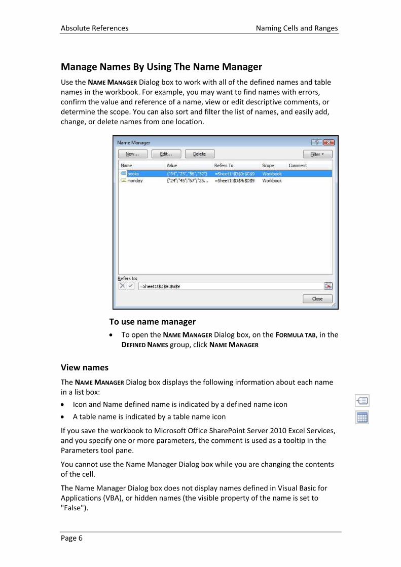
Use the NAME MANAGER Dialog box to work with all of the defined names and table names in the workbook. For example, you may want to find names with errors, confirm the value and reference of a name, view or edit descriptive comments, or determine the scope. You can also sort and filter the list of names, and easily add, change, or delete names from one location.
To use name manager
To open the NAME MANAGER Dialog box, on the FORMULA TAB, in the DEFINED NAMES group, click NAME MANAGER
View names
The NAME MANAGER Dialog box displays the following information about each name in a list box:
Icon and Name defined name is indicated by a defined name icon
A table name is indicated by a table name icon
If you save the workbook to Microsoft Office SharePoint Server 2010 Excel Services, and you specify one or more parameters, the comment is used as a tooltip in the Parameters tool pane.
You cannot use the Name Manager Dialog box while you are changing the contents of the cell.
The Name Manager Dialog box does not display names defined in Visual Basic for Applications (VBA), or hidden names (the visible property of the name is set to "False").
Excel Formulas and Functions.docx Naming Cells and Ranges
Page 7
Resize columns in name manager
To automatically size the column to fit the largest value in that column, double-click the right side of the column header or drag to left or right to adjust width
Sort names
To sort the list of names in ascending or descending order, alternately click the column header.
Filter names
Use the commands in the Filter drop-down list to quickly display a subset of names. Selecting each command toggles the filter operation on or off, which makes it easy to combine or remove different filter operations to get the results that you want.
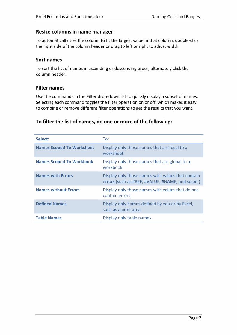
To filter the list of names, do one or more of the following:
Select: To:
Names Scoped To Worksheet Display only those names that are local to a worksheet.
Names Scoped To Workbook Display only those names that are global to a workbook.
Names with Errors Display only those names with values that contain errors (such as #REF, #VALUE, #NAME, and so on.)
Names without Errors Display only those names with values that do not contain errors.
Defined Names Display only names defined by you or by Excel, such as a print area.
Table Names Display only table names.
Absolute References Naming Cells and Ranges
Page 8
Changing a Name
To Change a name
On the FORMULAS TAB, in the DEFINED NAMES group, click NAME
MANAGER
In the NAME MANAGER Dialog box, click the name that you want to change, and then click EDIT. You can also double-click the name
The EDIT NAME dialog box is displayed
Type the new name for the reference in the Name box
Change the reference in the Refers to box, and click OK
In the NAME MANAGER Dialog box, in the REFERS TO box, change the cell, formula or constant represented by the name
To cancel unwanted or accidental changes, click CANCEL, or press ESC.
To save changes, click COMMIT , or press ENTER
If you change a defined name or table name, all uses of that name in the workbook are also changed. The Close button only closes the Name Manager Dialog box. It is not required to commit changes that have already been made
Delete one or more names
On the FORMULAS tab, in the DEFINED NAMES group, click NAME
MANAGER
In the NAME MANAGER dialog box, click the name that you want to change
To select a name click it
To select more than one name in a contiguous group, click and
drag the names, or press [SHIFT]+[Click] for each name in the
group
To select more than one name in a non-contiguous group, press
[CTRL]+[Click] for each name in the group
Click DELETE. You can also press DELETE.
Click OK to confirm the deletion.
The Close button only closes the Name Manager Dialog box. It is not required to commit changes that have already been made.
Excel Formulas and Functions.docx Naming Cells and Ranges
Page 9
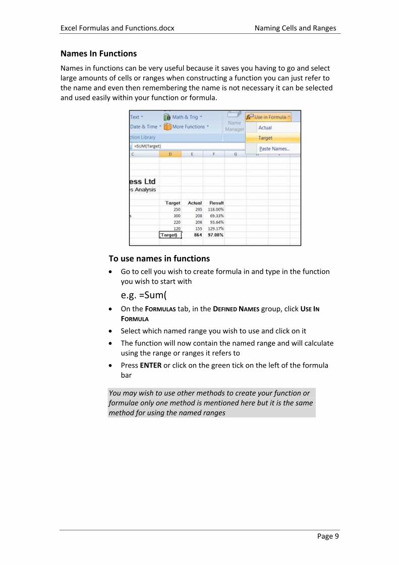
Names In Functions
Names in functions can be very useful because it saves you having to go and select large amounts of cells or ranges when constructing a function you can just refer to the name and even then remembering the name is not necessary it can be selected and used easily within your function or formula.
To use names in functions
Go to cell you wish to create formula in and type in the function you wish to start with
e.g. =Sum( On the FORMULAS tab, in the DEFINED NAMES group, click USE IN
FORMULA
Select which named range you wish to use and click on it
The function will now contain the named range and will calculate using the range or ranges it refers to
Press ENTER or click on the green tick on the left of the formula bar
You may wish to use other methods to create your function or formulae only one method is mentioned here but it is the same method for using the named ranges
Absolute References Naming Cells and Ranges
Page 10
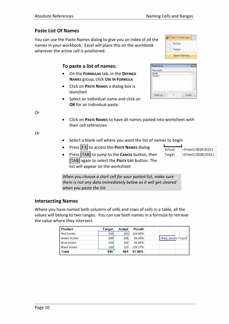
Paste List Of Names
You can use the Paste Names dialog to give you an index of all the names in your workbook. Excel will place this on the workbook wherever the active cell is positioned.
To paste a list of names:
On the FORMULAS tab, in the DEFINED
NAMES group, click USE IN FORMULA
Click on PASTE NAMES a dialog box is launched
Select an individual name and click on OK for an individual paste.
Or
Click on PASTE NAMES to have all names pasted into worksheet with their cell references
Or
Select a blank cell where you want the list of names to begin
Press [F3] to access the PASTE NAMES dialog
Press [TAB] to jump to the CANCEL button, then
[TAB] again to select the PASTE LIST button. The
list will appear on the worksheet
When you choose a start cell for your pasted list, make sure there is not any data immediately below as it will get cleared when you paste the list
Intersecting Names
Where you have named both columns of cells and rows of cells in a table, all the values will belong to two ranges. You can use both names in a formula to retrieve the value where they intersect.
Excel Formulas and Functions.docx Naming Cells and Ranges
Page 11
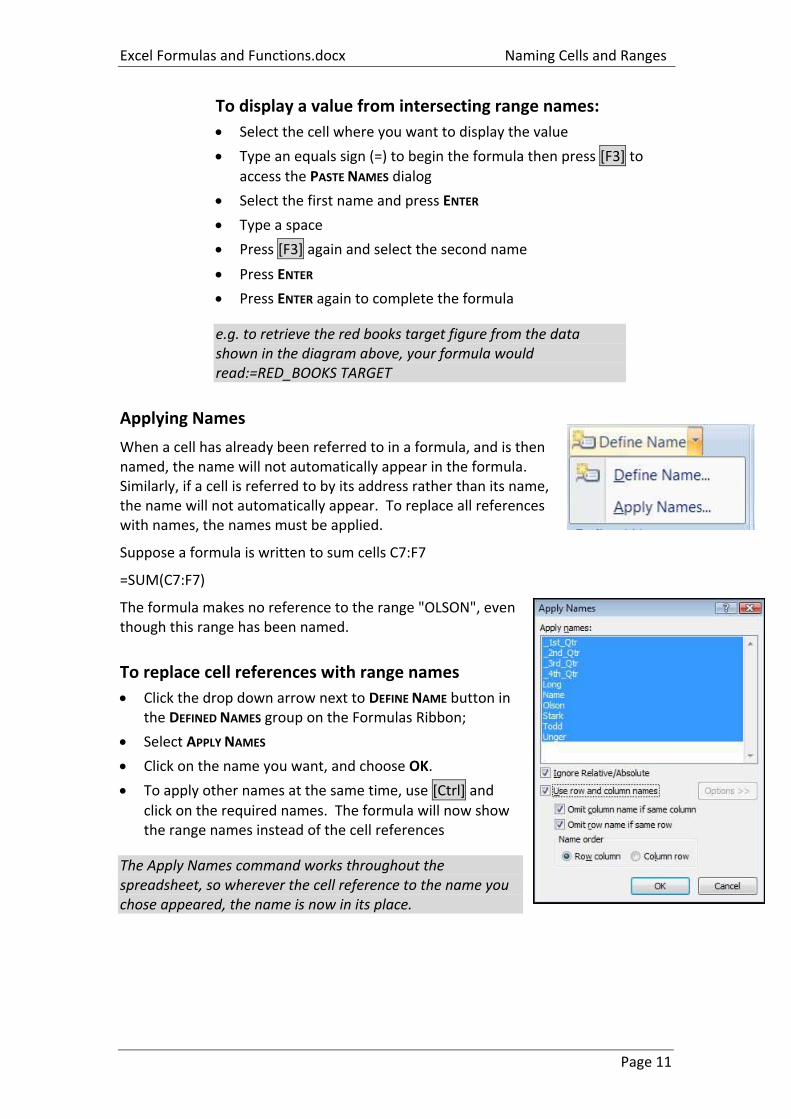
To display a value from intersecting range names:
Select the cell where you want to display the value
Type an equals sign (=) to begin the formula then press [F3] to
access the PASTE NAMES dialog
Select the first name and press ENTER
Type a space
Press [F3] again and select the second name
Press ENTER
Press ENTER again to complete the formula
e.g. to retrieve the red books target figure from the data shown in the diagram above, your formula would read:=RED_BOOKS TARGET
Applying Names
When a cell has already been referred to in a formula, and is then named, the name will not automatically appear in the formula. Similarly, if a cell is referred to by its address rather than its name, the name will not automatically appear. To replace all references with names, the names must be applied.
Suppose a formula is written to sum cells C7:F7
=SUM(C7:F7)
The formula makes no reference to the range "OLSON", even though this range has been named.
To replace cell references with range names
Click the drop down arrow next to DEFINE NAME button in the DEFINED NAMES group on the Formulas Ribbon;
Select APPLY NAMES
Click on the name you want, and choose OK.
To apply other names at the same time, use [Ctrl] and
click on the required names. The formula will now show the range names instead of the cell references
The Apply Names command works throughout the spreadsheet, so wherever the cell reference to the name you chose appeared, the name is now in its place.

Absolute References Naming Cells and Ranges
Page 12
Filtering out needed named ranges
Using the filter button allows some basic filtering of the names within your workbook
Don’t forget to clear the filter after you have what you want
Scoping is a function where the names may be used on a specific sheet or throughout the whole workbook. When filtering the names you have it may be useful to set a scope if you have many names on many sheets.
Excel Formulas and Functions.docx BoDMAS With Formulae
Page 13
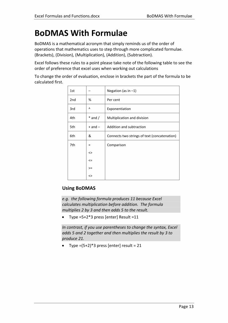
BoDMAS With Formulae BoDMAS is a mathematical acronym that simply reminds us of the order of operations that mathematics uses to step through more complicated formulae. (Brackets), (Division), (Multiplication), (Addition), (Subtraction).
Excel follows these rules to a point please take note of the following table to see the order of preference that excel uses when working out calculations
To change the order of evaluation, enclose in brackets the part of the formula to be calculated first.
1st – Negation (as in –1)
2nd % Per cent
3rd ^ Exponentiation
4th * and / Multiplication and division
5th + and – Addition and subtraction
6th & Connects two strings of text (concatenation)
7th =
<>
<=
>=
<>
Comparison
Using BoDMAS
e.g. the following formula produces 11 because Excel calculates multiplication before addition. The formula multiplies 2 by 3 and then adds 5 to the result.
Type =5+2*3 press [enter] Result =11
In contrast, if you use parentheses to change the syntax, Excel adds 5 and 2 together and then multiplies the result by 3 to produce 21.
Type =(5+2)*3 press [enter] result = 21
Absolute References Functions
Page 14
Functions
Basic Sum Function
Having mastered how to set up your own custom formulae, you will be able to carry out any calculations you wish. However, some calculations are complicated or involve referring to lots of cells making entry tedious and time consuming. For example, you could construct a formula to generate a total at the bottom of a column (or the end of a row), like this:
=D2+D3+D4+D5
The above formula would work, but if there were 400 cells to total and not just 4, you would get bored with entering the individual cell references.
When formulae become unwieldy or complex, Excel comes to the rescue with its own built-in formulae known as functions.
Functions always follow the same syntax:
The name of the selected function tells Excel what you want to do and the arguments generally tell Excel where the data is that you want to calculate.
Excel has a huge number of functions, not all of them are relevant to everyone. The functions are categorised according to what they do. In this manual, we outline some of the functions that can be usefully used at a general level.
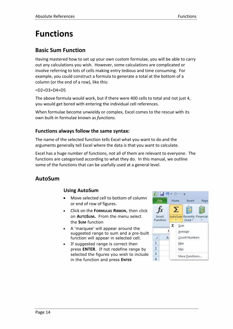
AutoSum
Using AutoSum
Move selected cell to bottom of column or end of row of figures.
Click on the FORMULAS RIBBON, then click
on AUTOSUM. From the menu select
the SUM function
A ‘marquee’ will appear around the
suggested range to sum and a pre-built
function will appear in selected cell.
If suggested range is correct then
press ENTER. If not redefine range by
selected the figures you wish to include
in the function and press ENTER
Excel Formulas and Functions.docx Functions
Page 15
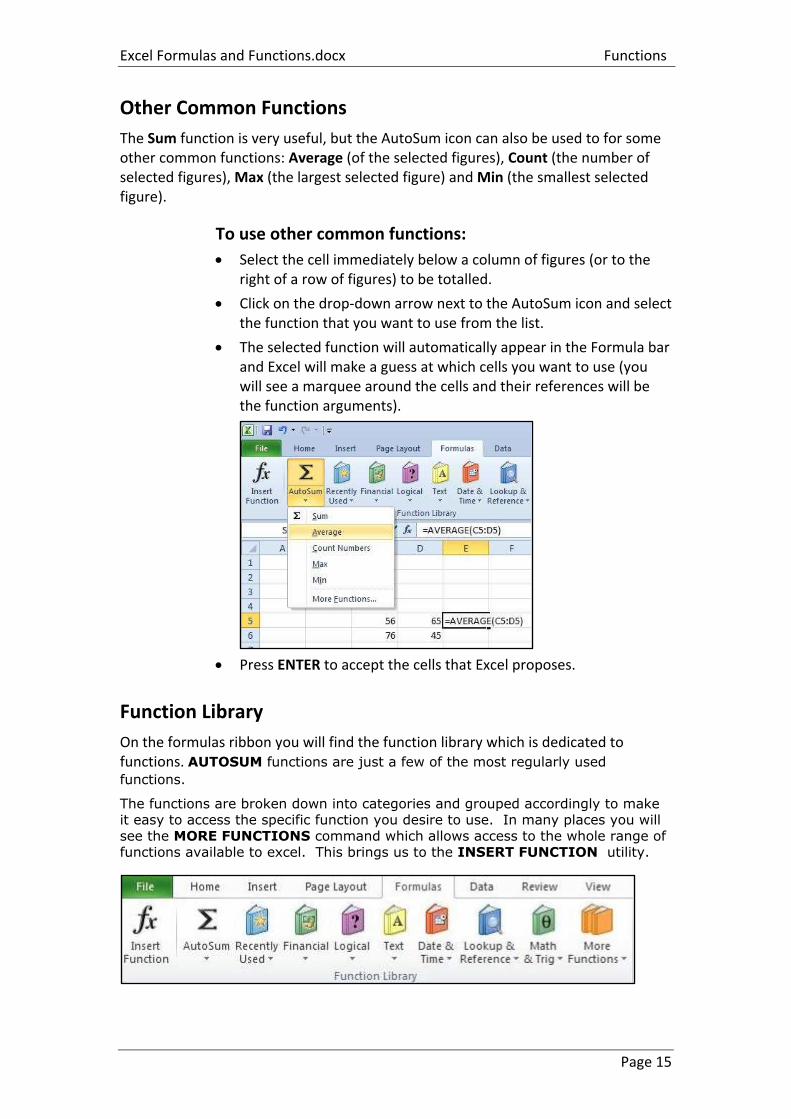
Other Common Functions
The Sum function is very useful, but the AutoSum icon can also be used to for some other common functions: Average (of the selected figures), Count (the number of selected figures), Max (the largest selected figure) and Min (the smallest selected figure).
To use other common functions:
Select the cell immediately below a column of figures (or to the right of a row of figures) to be totalled.
Click on the drop-down arrow next to the AutoSum icon and select the function that you want to use from the list.
The selected function will automatically appear in the Formula bar and Excel will make a guess at which cells you want to use (you will see a marquee around the cells and their references will be the function arguments).
Press ENTER to accept the cells that Excel proposes.
Function Library
On the formulas ribbon you will find the function library which is dedicated to functions. AUTOSUM functions are just a few of the most regularly used
functions.
The functions are broken down into categories and grouped accordingly to make it easy to access the specific function you desire to use. In many places you will
see the MORE FUNCTIONS command which allows access to the whole range of functions available to excel. This brings us to the INSERT FUNCTION utility.
Absolute References Functions
Page 16
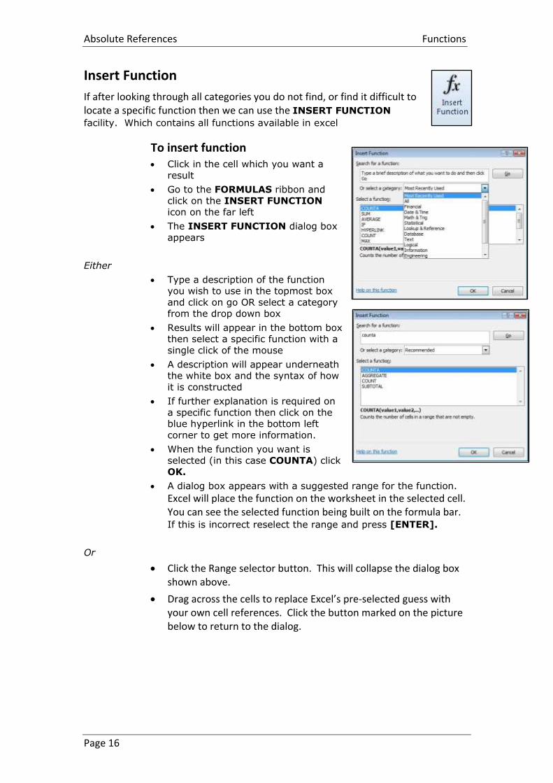
Insert Function
If after looking through all categories you do not find, or find it difficult to locate a specific function then we can use the INSERT FUNCTION
facility. Which contains all functions available in excel
To insert function
Click in the cell which you want a
result
Go to the FORMULAS ribbon and
click on the INSERT FUNCTION icon on the far left
The INSERT FUNCTION dialog box
appears
Either
Type a description of the function you wish to use in the topmost box
and click on go OR select a category from the drop down box
Results will appear in the bottom box then select a specific function with a
single click of the mouse
A description will appear underneath the white box and the syntax of how
it is constructed
If further explanation is required on
a specific function then click on the blue hyperlink in the bottom left
corner to get more information.
When the function you want is
selected (in this case COUNTA) click
OK.
A dialog box appears with a suggested range for the function. Excel will place the function on the worksheet in the selected cell. You can see the selected function being built on the formula bar. If this is incorrect reselect the range and press [ENTER].
Or
Click the Range selector button. This will collapse the dialog box shown above.
Drag across the cells to replace Excel’s pre-selected guess with your own cell references. Click the button marked on the picture below to return to the dialog.
Excel Formulas and Functions.docx Functions
Page 17
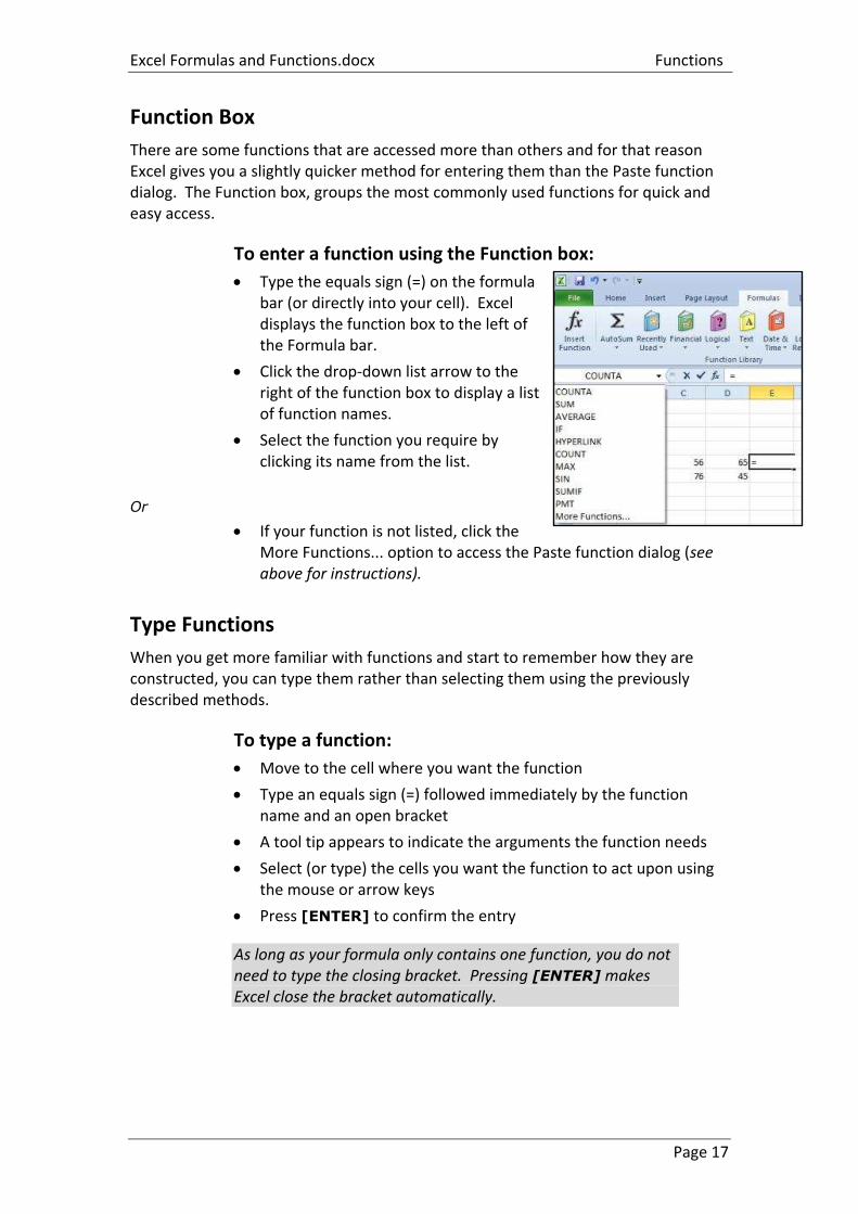
Function Box
There are some functions that are accessed more than others and for that reason Excel gives you a slightly quicker method for entering them than the Paste function dialog. The Function box, groups the most commonly used functions for quick and easy access.
To enter a function using the Function box:
Type the equals sign (=) on the formula bar (or directly into your cell). Excel displays the function box to the left of the Formula bar.
Click the drop-down list arrow to the right of the function box to display a list of function names.
Select the function you require by clicking its name from the list.
Or
If your function is not listed, click the More Functions... option to access the Paste function dialog (see above for instructions).
Type Functions
When you get more familiar with functions and start to remember how they are constructed, you can type them rather than selecting them using the previously described methods.
To type a function:
Move to the cell where you want the function
Type an equals sign (=) followed immediately by the function name and an open bracket
A tool tip appears to indicate the arguments the function needs
Select (or type) the cells you want the function to act upon using the mouse or arrow keys
Press [ENTER] to confirm the entry
As long as your formula only contains one function, you do not need to type the closing bracket. Pressing [ENTER] makes Excel close the bracket automatically.
Absolute References Functions
Page 18
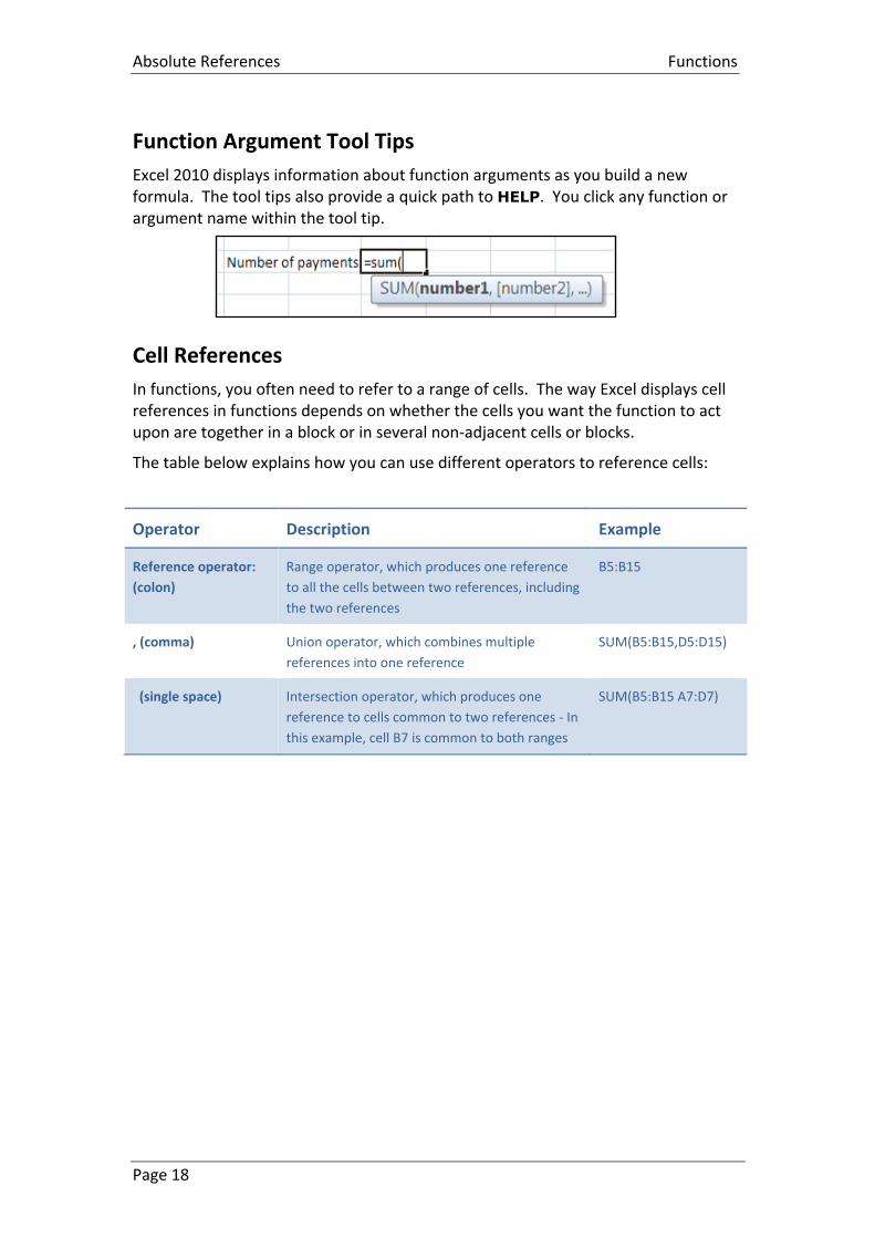
Function Argument Tool Tips
Excel 2010 displays information about function arguments as you build a new formula. The tool tips also provide a quick path to HELP. You click any function or argument name within the tool tip.
Cell References
In functions, you often need to refer to a range of cells. The way Excel displays cell references in functions depends on whether the cells you want the function to act upon are together in a block or in several non-adjacent cells or blocks.
The table below explains how you can use different operators to reference cells:
Operator Description Example
Reference operator:
(colon)
Range operator, which produces one reference
to all the cells between two references, including
the two references
B5:B15
, (comma) Union operator, which combines multiple
references into one reference
SUM(B5:B15,D5:D15)
(single space) Intersection operator, which produces one
reference to cells common to two references - In
this example, cell B7 is common to both ranges
SUM(B5:B15 A7:D7)
Excel Formulas and Functions.docx Conditional & Logical Functions
Page 19
Conditional & Logical Functions Excel has a number of logical functions which allow you to set various "conditions" and have data respond to them. For example, you may only want a certain calculation performed or piece of text displayed if certain conditions are met. The functions used to produce this type of analysis are found in the Insert, Function menu, under the heading LOGICAL.
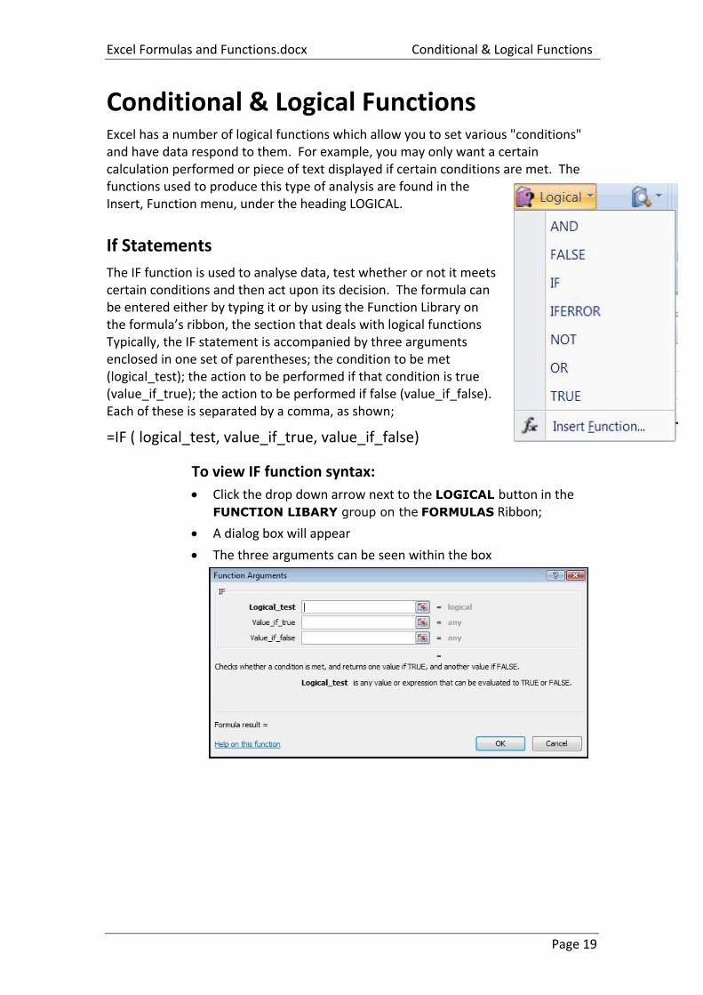
If Statements
The IF function is used to analyse data, test whether or not it meets certain conditions and then act upon its decision. The formula can be entered either by typing it or by using the Function Library on the formula’s ribbon, the section that deals with logical functions Typically, the IF statement is accompanied by three arguments enclosed in one set of parentheses; the condition to be met (logical_test); the action to be performed if that condition is true (value_if_true); the action to be performed if false (value_if_false). Each of these is separated by a comma, as shown;
=IF ( logical_test, value_if_true, value_if_false)
To view IF function syntax:
Click the drop down arrow next to the LOGICAL button in the FUNCTION LIBARY group on the FORMULAS Ribbon;
A dialog box will appear
The three arguments can be seen within the box
Absolute References Conditional & Logical Functions
Page 20
Logical Test
This part of the IF statement is the "condition", or test. You may want to test to see if a cell is a certain value, or to compare two cells. In these cases, symbols called LOGICAL OPERATORS are useful;
> Greater than
< Less than
> = Greater than or equal to
< = Less than or equal to
= Equal to
< > Not equal to
Therefore, a typical logical test might be B1 > B2, testing whether or not the value contained in cell B1 of the spreadsheet is greater than the value in cell B2. Names can also be included in the logical test, so if cells B1 and B2 were respectively named SALES and TARGET, the logical test would read SALES > TARGET. Another type of logical test could include text strings. If you want to check a cell to see if it contains text, that text string must be included in quotation marks. For example, cell C5 could be tested for the word YES as follows; C5="YES".
It should be noted that Excel's logic is, at times, brutally precise. In the above example, the logical test is that sales should be greater than target. If sales are equal to target, the IF statement will return the false value. To make the logical test more flexible, it would be advisable to use the operator > = to indicate "meeting or exceeding".
Value If True / False
Provided that you remember that TRUE value always precedes FALSE value, these two values can be almost anything. If desired, a simple number could be returned, a calculation performed, or even a piece of text entered. Also, the type of data entered can vary depending on whether it is a true or false result. You may want a calculation if the logical test is true, but a message displayed if false. (Remember that text to be included in functions should be enclosed in quotes).
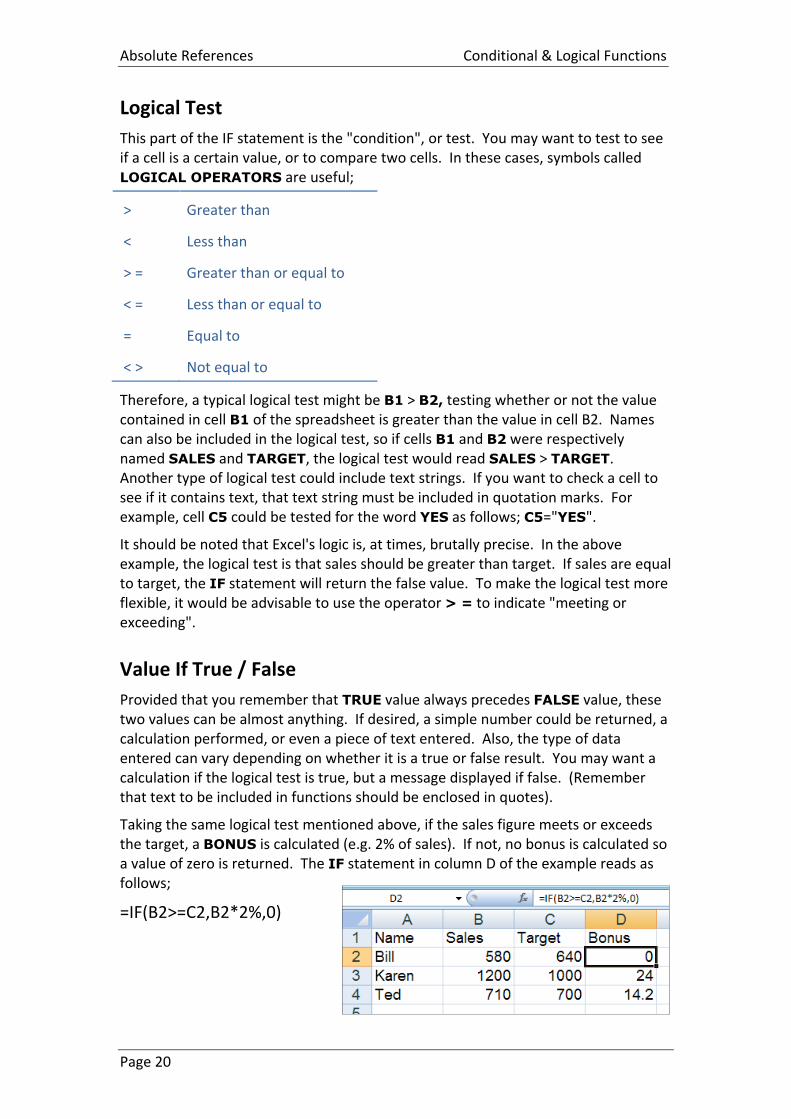
Taking the same logical test mentioned above, if the sales figure meets or exceeds the target, a BONUS is calculated (e.g. 2% of sales). If not, no bonus is calculated so a value of zero is returned. The IF statement in column D of the example reads as follows;
=IF(B2>=C2,B2*2%,0)
Excel Formulas and Functions.docx Conditional & Logical Functions
Page 21
You may, alternatively, want to see a message saying "NO BONUS". In this case, the true value will remain the same and the false value will be the text string "NO
BONUS";
=IF(B2>=C2,B2*2%,"NO BONUS")
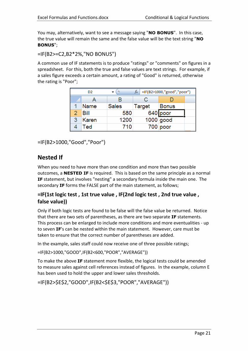
A common use of IF statements is to produce "ratings" or "comments" on figures in a spreadsheet. For this, both the true and false values are text strings. For example, if a sales figure exceeds a certain amount, a rating of "Good" is returned, otherwise the rating is "Poor";
=IF(B2>1000,"Good","Poor")
Nested If
When you need to have more than one condition and more than two possible outcomes, a NESTED IF is required. This is based on the same principle as a normal IF statement, but involves "nesting" a secondary formula inside the main one. The secondary IF forms the FALSE part of the main statement, as follows;
=IF(1st logic test , 1st true value , IF(2nd logic test , 2nd true value , false value))
Only if both logic tests are found to be false will the false value be returned. Notice that there are two sets of parentheses, as there are two separate IF statements. This process can be enlarged to include more conditions and more eventualities - up to seven IF's can be nested within the main statement. However, care must be taken to ensure that the correct number of parentheses are added.
In the example, sales staff could now receive one of three possible ratings;
=IF(B2>1000,"GOOD",IF(B2<600,"POOR","AVERAGE"))
To make the above IF statement more flexible, the logical tests could be amended to measure sales against cell references instead of figures. In the example, column E has been used to hold the upper and lower sales thresholds.
=IF(B2>$E$2,"GOOD",IF(B2<$E$3,"POOR","AVERAGE"))
Absolute References Conditional & Logical Functions
Page 22
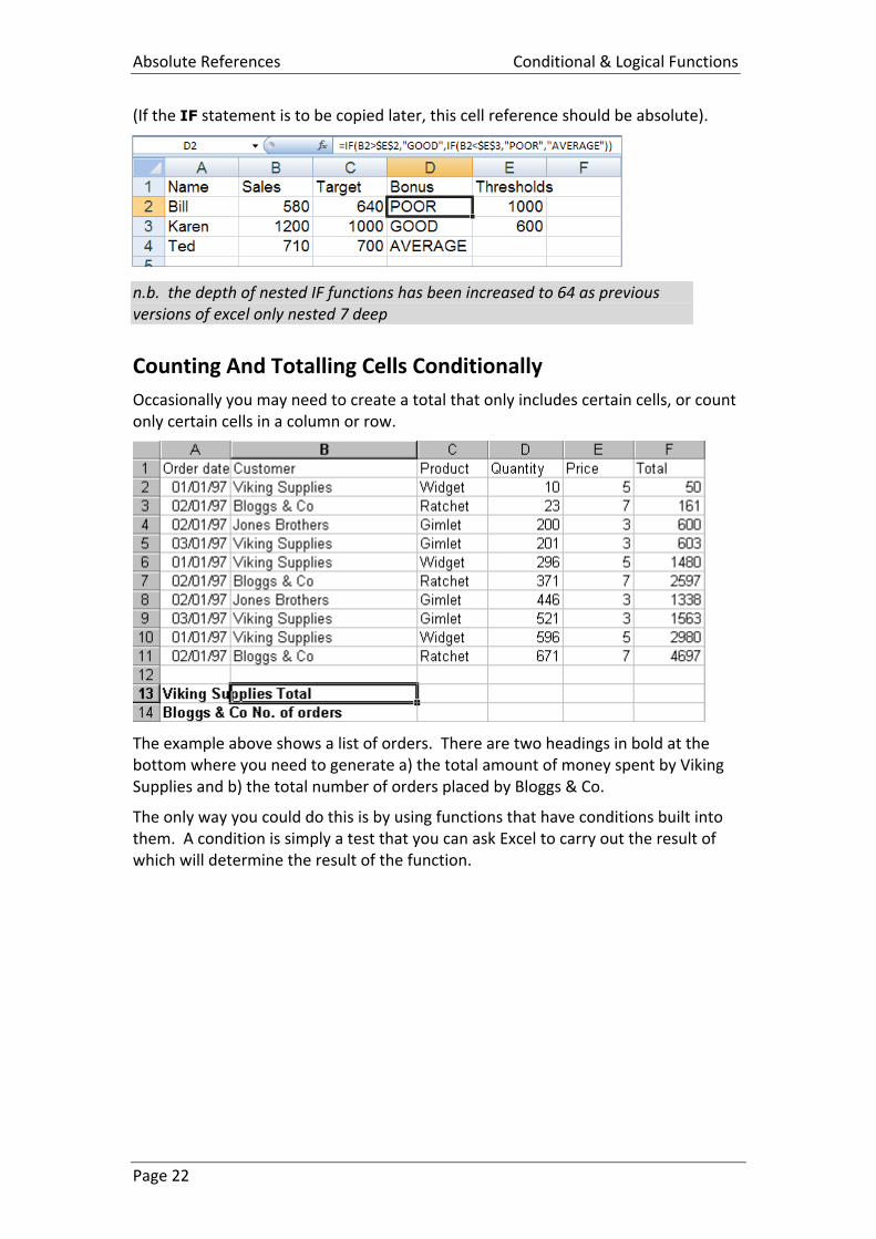
(If the IF statement is to be copied later, this cell reference should be absolute).
n.b. the depth of nested IF functions has been increased to 64 as previous versions of excel only nested 7 deep
Counting And Totalling Cells Conditionally
Occasionally you may need to create a total that only includes certain cells, or count only certain cells in a column or row.
The example above shows a list of orders. There are two headings in bold at the bottom where you need to generate a) the total amount of money spent by Viking Supplies and b) the total number of orders placed by Bloggs & Co.
The only way you could do this is by using functions that have conditions built into them. A condition is simply a test that you can ask Excel to carry out the result of which will determine the result of the function.
Excel Formulas and Functions.docx Conditional & Logical Functions
Page 23
Statistical If Statements
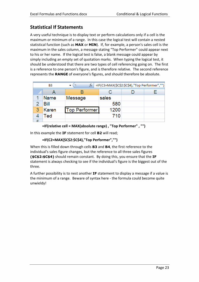
A very useful technique is to display text or perform calculations only if a cell is the maximum or minimum of a range. In this case the logical test will contain a nested statistical function (such as MAX or MIN). If, for example, a person's sales cell is the maximum in the sales column, a message stating "Top Performer" could appear next to his or her name. If the logical test is false, a blank message could appear by simply including an empty set of quotation marks. When typing the logical test, it should be understood that there are two types of cell referencing going on. The first is a reference to one person's figure, and is therefore relative. The second reference represents the RANGE of everyone's figures, and should therefore be absolute.
=IF(relative cell = MAX(absolute range) , "Top Performer" , "")
In this example the IF statement for cell B2 will read;
=IF(C2=MAX($C$2:$C$4),"Top Performer","")
When this is filled down through cells B3 and B4, the first reference to the individual's sales figure changes, but the reference to all three sales figures ($C$2:$C$4) should remain constant. By doing this, you ensure that the IF statement is always checking to see if the individual's figure is the biggest out of the three.
A further possibility is to nest another IF statement to display a message if a value is the minimum of a range. Beware of syntax here - the formula could become quite unwieldy!
Absolute References Conditional & Logical Functions
Page 24
Sumif
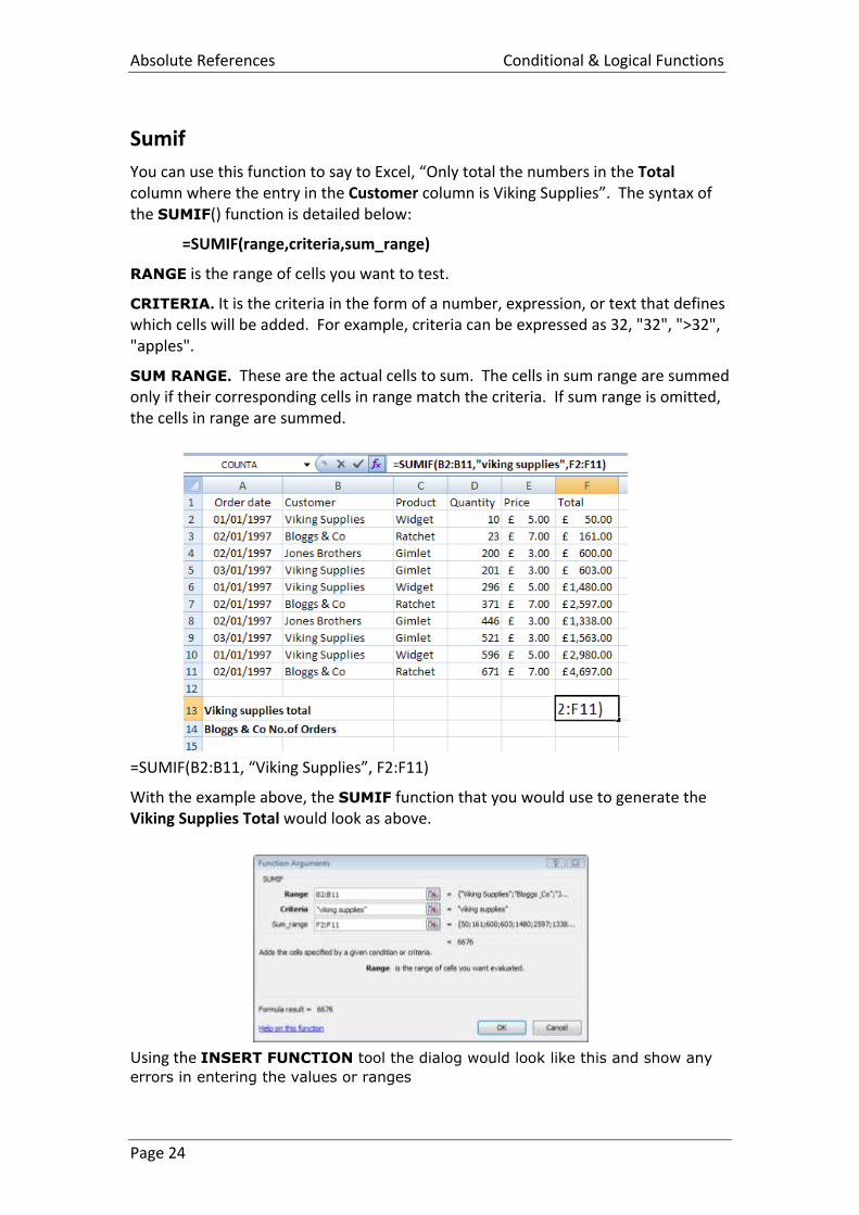
You can use this function to say to Excel, “Only total the numbers in the Total column where the entry in the Customer column is Viking Supplies”. The syntax of the SUMIF() function is detailed below:
=SUMIF(range,criteria,sum_range)
RANGE is the range of cells you want to test.
CRITERIA. It is the criteria in the form of a number, expression, or text that defines which cells will be added. For example, criteria can be expressed as 32, "32", ">32", "apples".
SUM RANGE. These are the actual cells to sum. The cells in sum range are summed only if their corresponding cells in range match the criteria. If sum range is omitted, the cells in range are summed.
=SUMIF(B2:B11, “Viking Supplies”, F2:F11)
With the example above, the SUMIF function that you would use to generate the Viking Supplies Total would look as above.
Using the INSERT FUNCTION tool the dialog would look like this and show any
errors in entering the values or ranges
Excel Formulas and Functions.docx Conditional & Logical Functions
Page 25
Countif
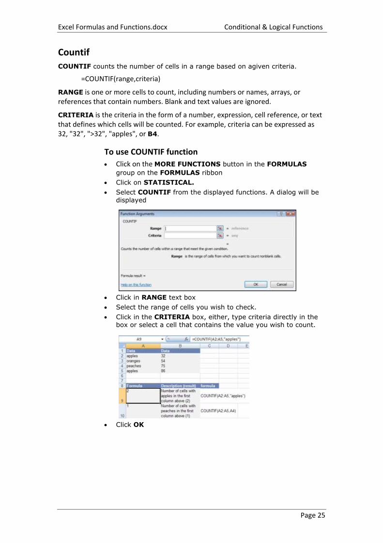
COUNTIF counts the number of cells in a range based on agiven criteria.
=COUNTIF(range,criteria)
RANGE is one or more cells to count, including numbers or names, arrays, or references that contain numbers. Blank and text values are ignored.
CRITERIA is the criteria in the form of a number, expression, cell reference, or text that defines which cells will be counted. For example, criteria can be expressed as 32, "32", ">32", "apples", or B4.
To use COUNTIF function
Click on the MORE FUNCTIONS button in the FORMULAS
group on the FORMULAS ribbon
Click on STATISTICAL.
Select COUNTIF from the displayed functions. A dialog will be
displayed
Click in RANGE text box
Select the range of cells you wish to check.
Click in the CRITERIA box, either, type criteria directly in the box or select a cell that contains the value you wish to count.
Click OK
Absolute References Conditional & Logical Functions
Page 26
Averageif
A common request is for a single function to conditionally average a range of numbers – a complement to SUMIF and COUNTIF. AVERAGEIF, allows users to easily average a range based on a specific criteria.
=AVERAGEIF(Range, Criteria, [Average Range])
RANGE is one or more cells to average, including numbers or names, arrays, or references that contain numbers.
CRITERIA is the criteria in the form of a number, expression, cell reference, or text that defines which cells are averaged. For example, criteria can be expressed as 32, "32", ">32", "apples", or B4.
AVERAGE_range is the actual set of cells to average. If omitted, RANGE is used.
Here is an example that returns the average of B2:B5 where the corresponding value in column A is greater than 250,000:
=AVERAGEIF(A2:A5, “>250000”, B2:B5)
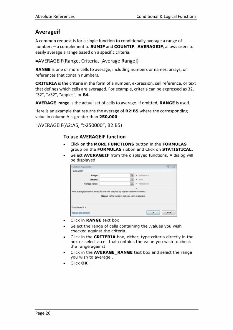
To use AVERAGEIF function
Click on the MORE FUNCTIONS button in the FORMULAS
group on the FORMULAS ribbon and Click on STATISTICAL.
Select AVERAGEIF from the displayed functions. A dialog will
be displayed
Click in RANGE text box
Select the range of cells containing the .values you wish
checked against the criteria.
Click in the CRITERIA box, either, type criteria directly in the
box or select a cell that contains the value you wish to check the range against
Click in the AVERAGE_RANGE text box and select the range
you wish to average..
Click OK
Excel Formulas and Functions.docx Conditional & Logical Functions
Page 27
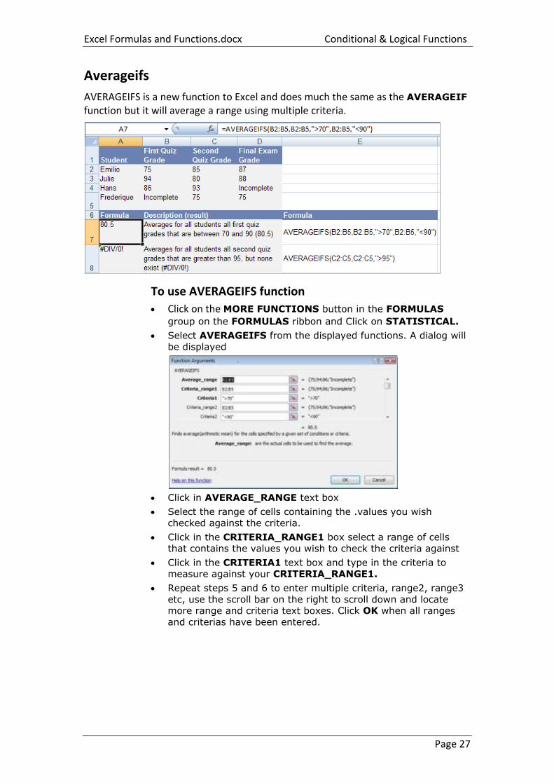
Averageifs
AVERAGEIFS is a new function to Excel and does much the same as the AVERAGEIF function but it will average a range using multiple criteria.
To use AVERAGEIFS function
Click on the MORE FUNCTIONS button in the FORMULAS
group on the FORMULAS ribbon and Click on STATISTICAL.
Select AVERAGEIFS from the displayed functions. A dialog will
be displayed
Click in AVERAGE_RANGE text box
Select the range of cells containing the .values you wish
checked against the criteria.
Click in the CRITERIA_RANGE1 box select a range of cells
that contains the values you wish to check the criteria against
Click in the CRITERIA1 text box and type in the criteria to
measure against your CRITERIA_RANGE1.
Repeat steps 5 and 6 to enter multiple criteria, range2, range3
etc, use the scroll bar on the right to scroll down and locate more range and criteria text boxes. Click OK when all ranges
and criterias have been entered.
Absolute References Conditional & Logical Functions
Page 28
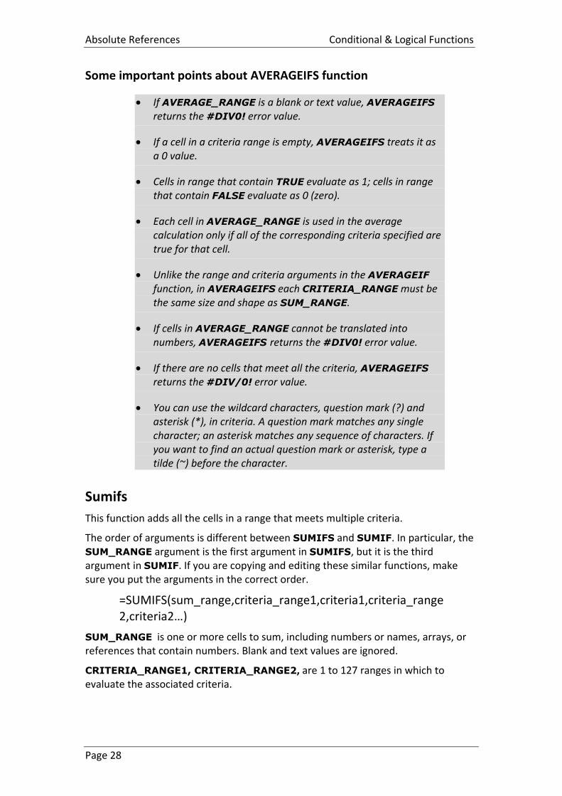
Some important points about AVERAGEIFS function
If AVERAGE_RANGE is a blank or text value, AVERAGEIFS returns the #DIV0! error value.
If a cell in a criteria range is empty, AVERAGEIFS treats it as a 0 value.
Cells in range that contain TRUE evaluate as 1; cells in range that contain FALSE evaluate as 0 (zero).
Each cell in AVERAGE_RANGE is used in the average calculation only if all of the corresponding criteria specified are true for that cell.
Unlike the range and criteria arguments in the AVERAGEIF function, in AVERAGEIFS each CRITERIA_RANGE must be the same size and shape as SUM_RANGE.
If cells in AVERAGE_RANGE cannot be translated into numbers, AVERAGEIFS returns the #DIV0! error value.
If there are no cells that meet all the criteria, AVERAGEIFS
returns the #DIV/0! error value.
You can use the wildcard characters, question mark (?) and asterisk (*), in criteria. A question mark matches any single character; an asterisk matches any sequence of characters. If you want to find an actual question mark or asterisk, type a tilde (~) before the character.
Sumifs
This function adds all the cells in a range that meets multiple criteria.
The order of arguments is different between SUMIFS and SUMIF. In particular, the SUM_RANGE argument is the first argument in SUMIFS, but it is the third argument in SUMIF. If you are copying and editing these similar functions, make sure you put the arguments in the correct order.
=SUMIFS(sum_range,criteria_range1,criteria1,criteria_range2,criteria2…)
SUM_RANGE is one or more cells to sum, including numbers or names, arrays, or references that contain numbers. Blank and text values are ignored.
CRITERIA_RANGE1, CRITERIA_RANGE2, are 1 to 127 ranges in which to evaluate the associated criteria.
Excel Formulas and Functions.docx Conditional & Logical Functions
Page 29
CRITERIA1, CRITERIA2, …are 1 to 127 criteria in the form of a number, expression, cell reference, or text that define which cells will be added. For example, criteria can be expressed as 32, "32", ">32", "apples", or B4.
Some important points about SUMIFS
Each cell in SUM_RANGE is summed only if all of the corresponding criteria specified are true for that cell.
Cells in SUM_RANGE that contain TRUE evaluate as 1; cells in SUM_RANGE that contain FALSE evaluate as 0 (zero).
Unlike the range and criteria arguments in the SUMIF function, in SUMIFS each CRITERIA_RANGE must be the same size and shape as SUM_RANGE.
You can use the wildcard characters, question mark (?) and asterisk (*), in criteria. A question mark matches any single character; an asterisk matches any sequence of characters. If you want to find an actual question mark or asterisk, type a tilde (~) before the character.
To use SUMIFS function
Click on the MATH & TRIG BUTTON in the FORMULAS group
on the FORMULAS ribbon.
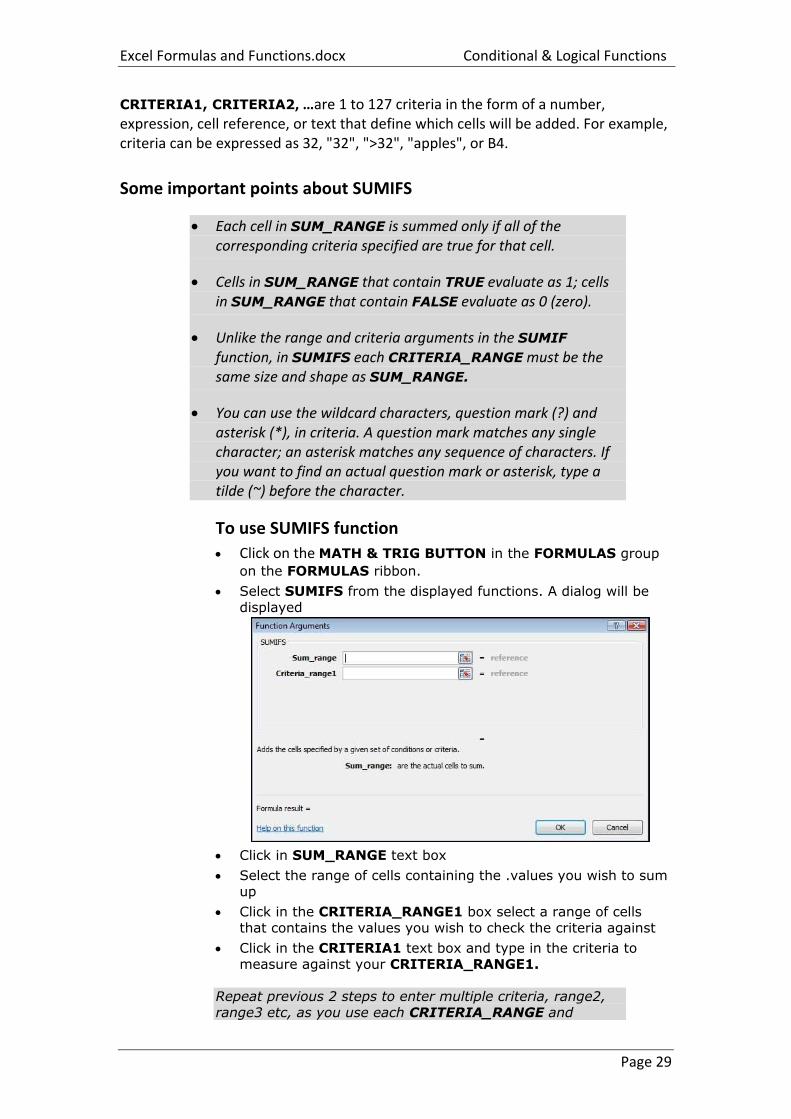
Select SUMIFS from the displayed functions. A dialog will be
displayed
Click in SUM_RANGE text box
Select the range of cells containing the .values you wish to sum up
Click in the CRITERIA_RANGE1 box select a range of cells that contains the values you wish to check the criteria against
Click in the CRITERIA1 text box and type in the criteria to measure against your CRITERIA_RANGE1.
Repeat previous 2 steps to enter multiple criteria, range2, range3 etc, as you use each CRITERIA_RANGE and
Absolute References Conditional & Logical Functions
Page 30
CRITERIA more text boxes will appear for you to use. Click
OK when all ranges and criterias have been entered.
Countifs
The COUNTIFS function, counts a range based on multiple criteria.
=COUNTIFS(range1, criteria1,range2, criteria2…)
RANGE1, RANGE2, … are 1 to 127 ranges in which to evaluate the associated criteria. Cells in each range must be numbers or names, arrays, or references that contain numbers. Blank and text values are ignored.
CRITERIA1, CRITERIA2, …are 1 to 127 criteria in the form of a number, expression, cell reference, or text that define which cells will be counted. For example, criteria can be expressed as 32, "32", ">32", "apples", or B4.
Excel Formulas and Functions.docx Conditional & Logical Functions
Page 31
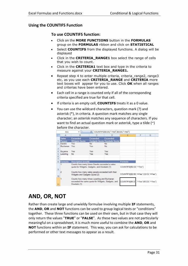
Using the COUNTIFS Function
To use COUNTIFS function:
Click on the MORE FUNCTIONS button in the FORMULAS
group on the FORMULAS ribbon and click on STATISTICAL
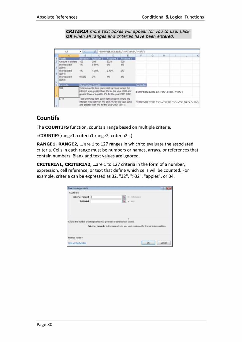
Select COUNTIFS from the displayed functions. A dialog will be
displayed
Click in the CRITERIA_RANGE1 box select the range of cells
that you wish to count.
Click in the CRITERIA1 text box and type in the criteria to measure against your CRITERIA_RANGE1.
Repeat step 4 to enter multiple criteria, criteria_range2, range3 etc, as you use each CRITERIA_RANGE and CRITERIA more text boxes will appear for you to use. Click OK when all ranges
and criterias have been entered.
Each cell in a range is counted only if all of the corresponding criteria specified are true for that cell.
If criteria is an empty cell, COUNTIFS treats it as a 0 value.
You can use the wildcard characters, question mark (?) and asterisk (*), in criteria. A question mark matches any single character; an asterisk matches any sequence of characters. If you want to find an actual question mark or asterisk, type a tilde (~) before the character.
AND, OR, NOT Rather than create large and unwieldy formulae involving multiple IF statements, the AND, OR and NOT functions can be used to group logical tests or "conditions" together. These three functions can be used on their own, but in that case they will only return the values "TRUE" or "FALSE". As these two values are not particularly meaningful on a spreadsheet, it is much more useful to combine the AND, OR and NOT functions within an IF statement. This way, you can ask for calculations to be performed or other text messages to appear as a result.
AND, OR, NOT Conditional & Logical Functions
Page 32
And Function
This function is a logical test to see if all conditions are true. If this is the case, the value "TRUE" is returned. If any of the arguments in the AND statement are found to be false, the whole statement produces the value "FALSE". This function is particularly useful as a check to make sure that all conditions you set are met.
Arguments are entered in the AND statement in parentheses, separated by commas, and there is a maximum of 30 arguments to one AND statement. The following example checks that two cells, B1 and B2, are both greater than 100.
=AND(B1>100,B2>100)
If either one of these two cells contains a value less than a hundred, the result of the AND statement is "FALSE.” This can now be wrapped inside an IF function to produce a more meaningful result. You may want to add the two figures together if they are over 100, or display a message indicating that they are not high enough.
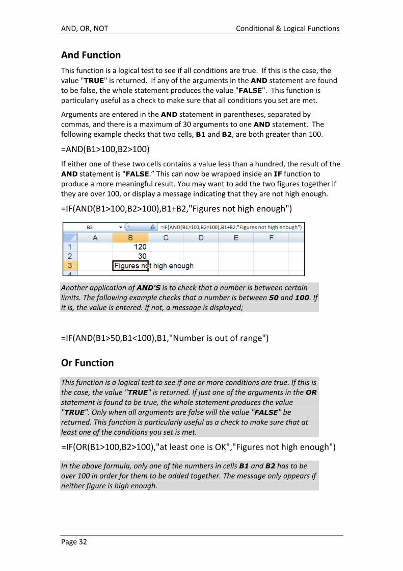
=IF(AND(B1>100,B2>100),B1+B2,"Figures not high enough")
Another application of AND'S is to check that a number is between certain limits. The following example checks that a number is between 50 and 100. If it is, the value is entered. If not, a message is displayed;
=IF(AND(B1>50,B1<100),B1,"Number is out of range")
Or Function
This function is a logical test to see if one or more conditions are true. If this is the case, the value "TRUE" is returned. If just one of the arguments in the OR statement is found to be true, the whole statement produces the value "TRUE". Only when all arguments are false will the value "FALSE" be returned. This function is particularly useful as a check to make sure that at least one of the conditions you set is met.
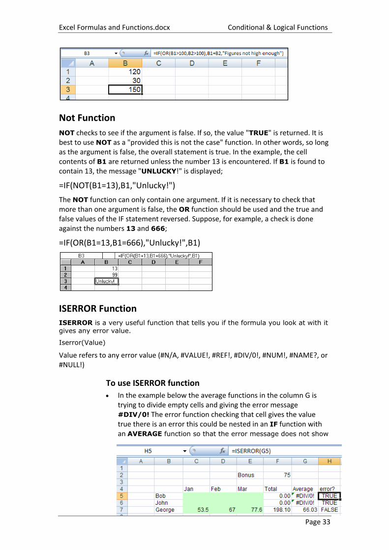
=IF(OR(B1>100,B2>100),"at least one is OK","Figures not high enough")
In the above formula, only one of the numbers in cells B1 and B2 has to be over 100 in order for them to be added together. The message only appears if neither figure is high enough.
Excel Formulas and Functions.docx Conditional & Logical Functions
Page 33
Not Function
NOT checks to see if the argument is false. If so, the value "TRUE" is returned. It is best to use NOT as a "provided this is not the case" function. In other words, so long as the argument is false, the overall statement is true. In the example, the cell contents of B1 are returned unless the number 13 is encountered. If B1 is found to contain 13, the message "UNLUCKY!" is displayed;
=IF(NOT(B1=13),B1,"Unlucky!")
The NOT function can only contain one argument. If it is necessary to check that more than one argument is false, the OR function should be used and the true and false values of the IF statement reversed. Suppose, for example, a check is done against the numbers 13 and 666;
=IF(OR(B1=13,B1=666),"Unlucky!",B1)
ISERROR Function
ISERROR is a very useful function that tells you if the formula you look at with it
gives any error value.
Iserror(Value)
Value refers to any error value (#N/A, #VALUE!, #REF!, #DIV/0!, #NUM!, #NAME?, or #NULL!)
To use ISERROR function
In the example below the average functions in the column G is trying to divide empty cells and giving the error message #DIV/0! The error function checking that cell gives the value true there is an error this could be nested in an IF function with an AVERAGE function so that the error message does not show
AND, OR, NOT Conditional & Logical Functions
Page 34
in column G
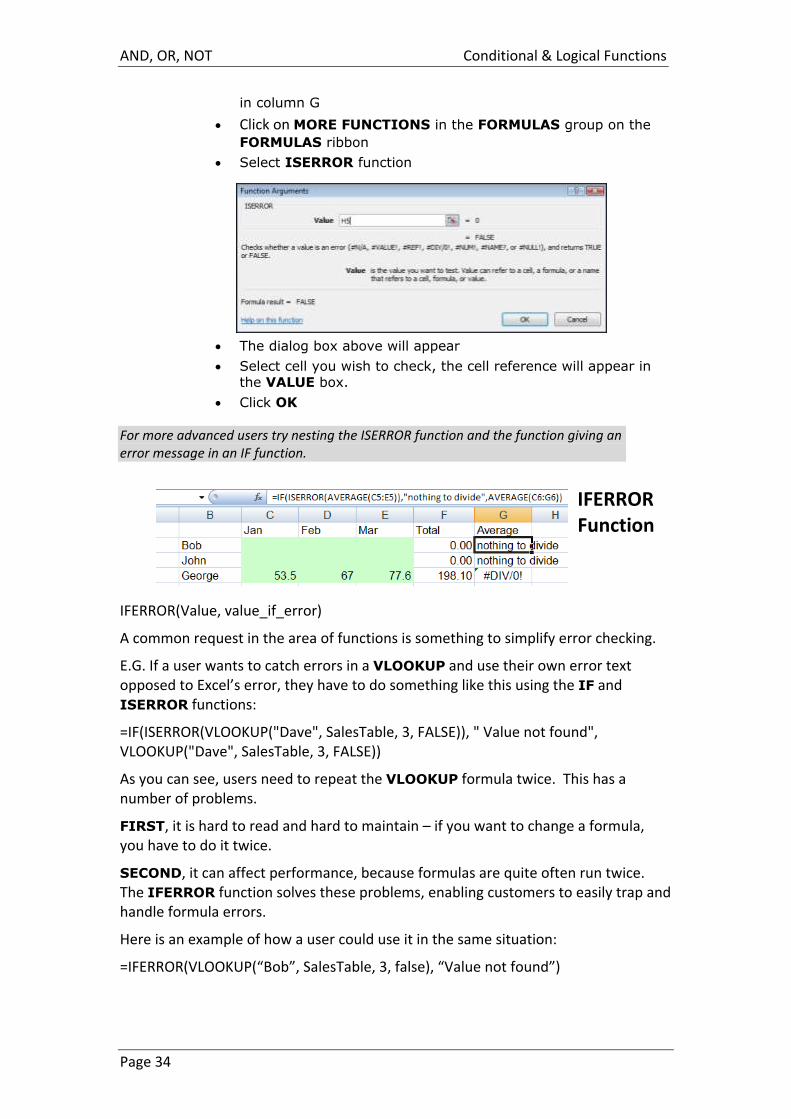
Click on MORE FUNCTIONS in the FORMULAS group on the
FORMULAS ribbon
Select ISERROR function
The dialog box above will appear
Select cell you wish to check, the cell reference will appear in the VALUE box.
Click OK
For more advanced users try nesting the ISERROR function and the function giving an error message in an IF function.
IFERROR Function
IFERROR(Value, value_if_error)
A common request in the area of functions is something to simplify error checking.
E.G. If a user wants to catch errors in a VLOOKUP and use their own error text opposed to Excel’s error, they have to do something like this using the IF and ISERROR functions:
=IF(ISERROR(VLOOKUP("Dave", SalesTable, 3, FALSE)), " Value not found", VLOOKUP("Dave", SalesTable, 3, FALSE))
As you can see, users need to repeat the VLOOKUP formula twice. This has a number of problems.
FIRST, it is hard to read and hard to maintain – if you want to change a formula, you have to do it twice.
SECOND, it can affect performance, because formulas are quite often run twice. The IFERROR function solves these problems, enabling customers to easily trap and handle formula errors.
Here is an example of how a user could use it in the same situation:
=IFERROR(VLOOKUP(“Bob”, SalesTable, 3, false), “Value not found”)
Excel Formulas and Functions.docx Conditional & Logical Functions
Page 35
To use IFERROR function
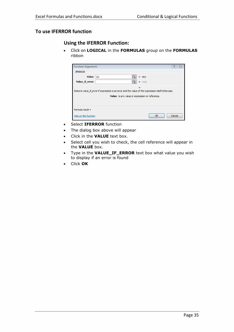
Using the IFERROR Function:
Click on LOGICAL in the FORMULAS group on the FORMULAS
ribbon
Select IFERROR function
The dialog box above will appear
Click in the VALUE text box.
Select cell you wish to check, the cell reference will appear in the VALUE box.
Type in the VALUE_IF_ERROR text box what value you wish to display if an error is found
Click OK
Lookup Functions Conditional & Logical Functions
Page 36
Lookup Functions As already mentioned, Excel can produce varying results in a cell, depending on conditions set by you. For example, if numbers are above or below certain limits, different calculations will be performed and text messages displayed. The usual method for constructing this sort of analysis is using the IF function. However, as already demonstrated, this can become large and unwieldy when you want multiple conditions and many possible outcomes. To begin with, Excel can only nest seven IF clauses in a main IF statement, whereas you may want more than eight logical tests or "scenarios.” To achieve this, Excel provides some LOOKUP functions. These functions allow you to create formulae which examine large amounts of data and find information which matches or approximates to certain conditions. They are simpler to construct than nested IF’s and can produce many more varied results.
Lookup
Before you actually start to use the various LOOKUP functions, it is worth learning the terms that you will come across, what they mean and the syntax of the function arguments.
Vector Lookup
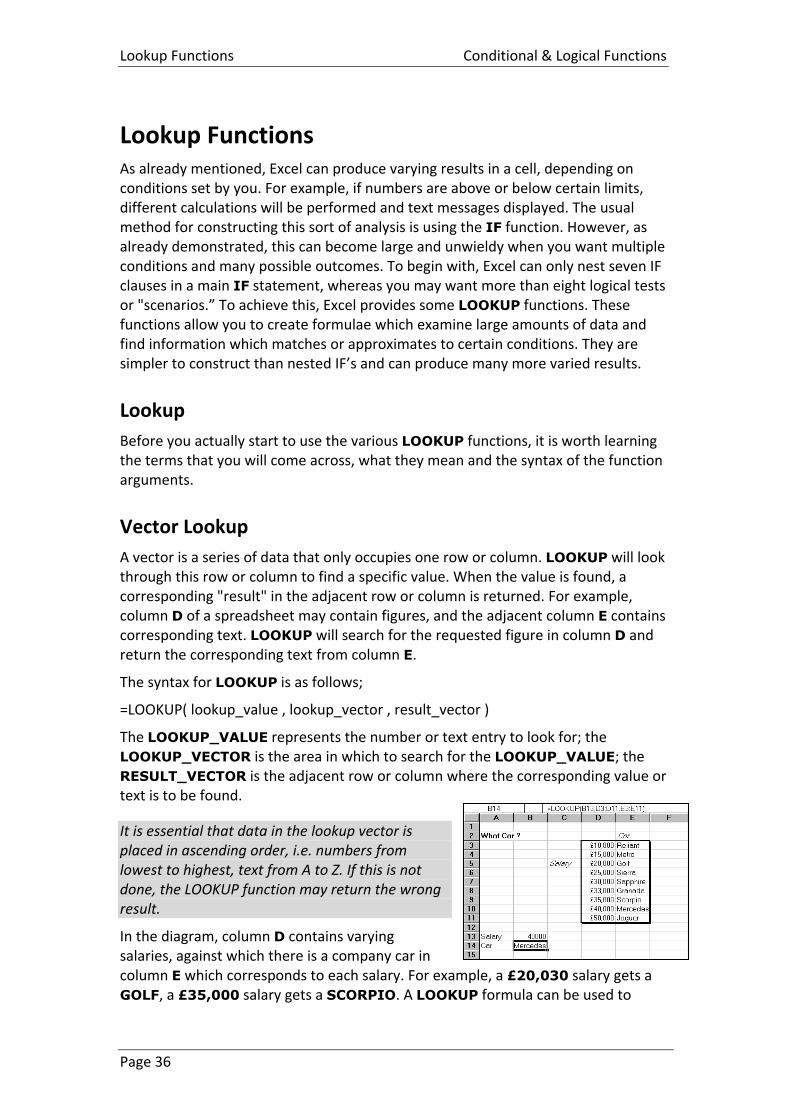
A vector is a series of data that only occupies one row or column. LOOKUP will look through this row or column to find a specific value. When the value is found, a corresponding "result" in the adjacent row or column is returned. For example, column D of a spreadsheet may contain figures, and the adjacent column E contains corresponding text. LOOKUP will search for the requested figure in column D and return the corresponding text from column E.
The syntax for LOOKUP is as follows;
=LOOKUP( lookup_value , lookup_vector , result_vector )
The LOOKUP_VALUE represents the number or text entry to look for; the LOOKUP_VECTOR is the area in which to search for the LOOKUP_VALUE; the RESULT_VECTOR is the adjacent row or column where the corresponding value or text is to be found.
It is essential that data in the lookup vector is placed in ascending order, i.e. numbers from lowest to highest, text from A to Z. If this is not done, the LOOKUP function may return the wrong result.
In the diagram, column D contains varying salaries, against which there is a company car in column E which corresponds to each salary. For example, a £20,030 salary gets a GOLF, a £35,000 salary gets a SCORPIO. A LOOKUP formula can be used to
Excel Formulas and Functions.docx Conditional & Logical Functions
Page 37
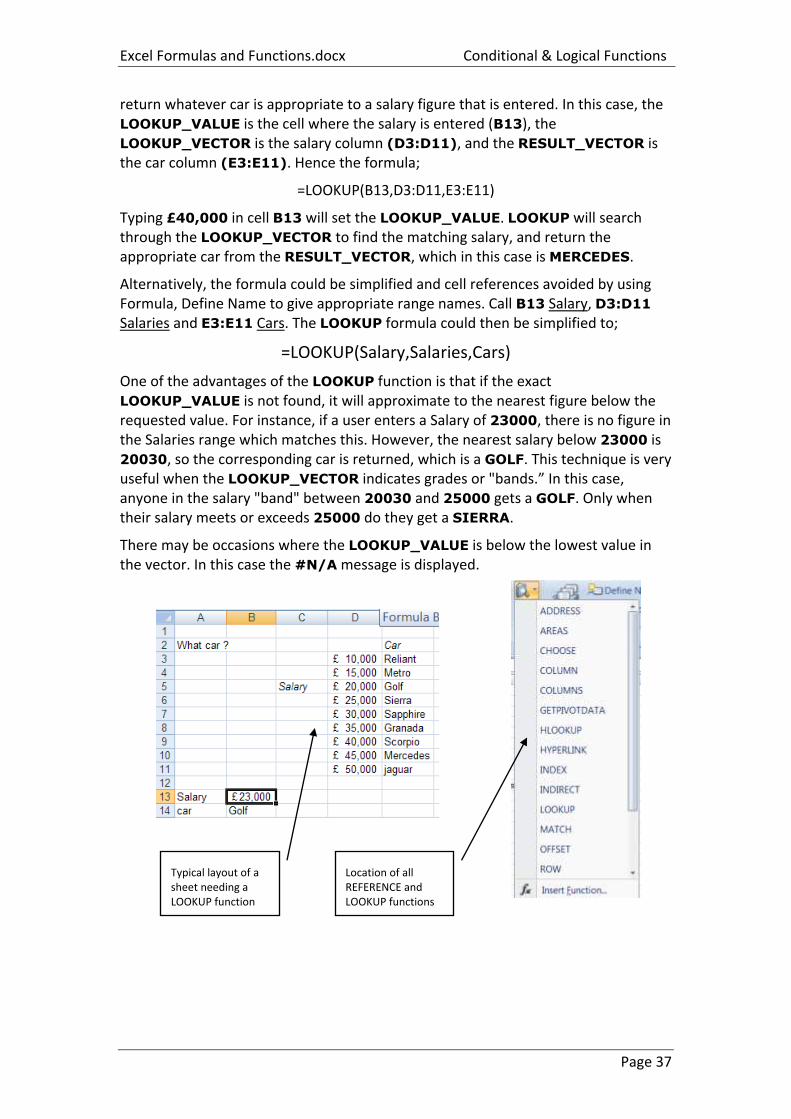
return whatever car is appropriate to a salary figure that is entered. In this case, the LOOKUP_VALUE is the cell where the salary is entered (B13), the LOOKUP_VECTOR is the salary column (D3:D11), and the RESULT_VECTOR is the car column (E3:E11). Hence the formula;
=LOOKUP(B13,D3:D11,E3:E11)
Typing £40,000 in cell B13 will set the LOOKUP_VALUE. LOOKUP will search through the LOOKUP_VECTOR to find the matching salary, and return the appropriate car from the RESULT_VECTOR, which in this case is MERCEDES.
Alternatively, the formula could be simplified and cell references avoided by using Formula, Define Name to give appropriate range names. Call B13 Salary, D3:D11 Salaries and E3:E11 Cars. The LOOKUP formula could then be simplified to;
=LOOKUP(Salary,Salaries,Cars)
One of the advantages of the LOOKUP function is that if the exact LOOKUP_VALUE is not found, it will approximate to the nearest figure below the requested value. For instance, if a user enters a Salary of 23000, there is no figure in the Salaries range which matches this. However, the nearest salary below 23000 is 20030, so the corresponding car is returned, which is a GOLF. This technique is very useful when the LOOKUP_VECTOR indicates grades or "bands.” In this case, anyone in the salary "band" between 20030 and 25000 gets a GOLF. Only when their salary meets or exceeds 25000 do they get a SIERRA.
There may be occasions where the LOOKUP_VALUE is below the lowest value in the vector. In this case the #N/A message is displayed.
Location of all REFERENCE and LOOKUP functions
Typical layout of a sheet needing a LOOKUP function
Lookup Functions Conditional & Logical Functions
Page 38
Inserting a LOOKUP Function
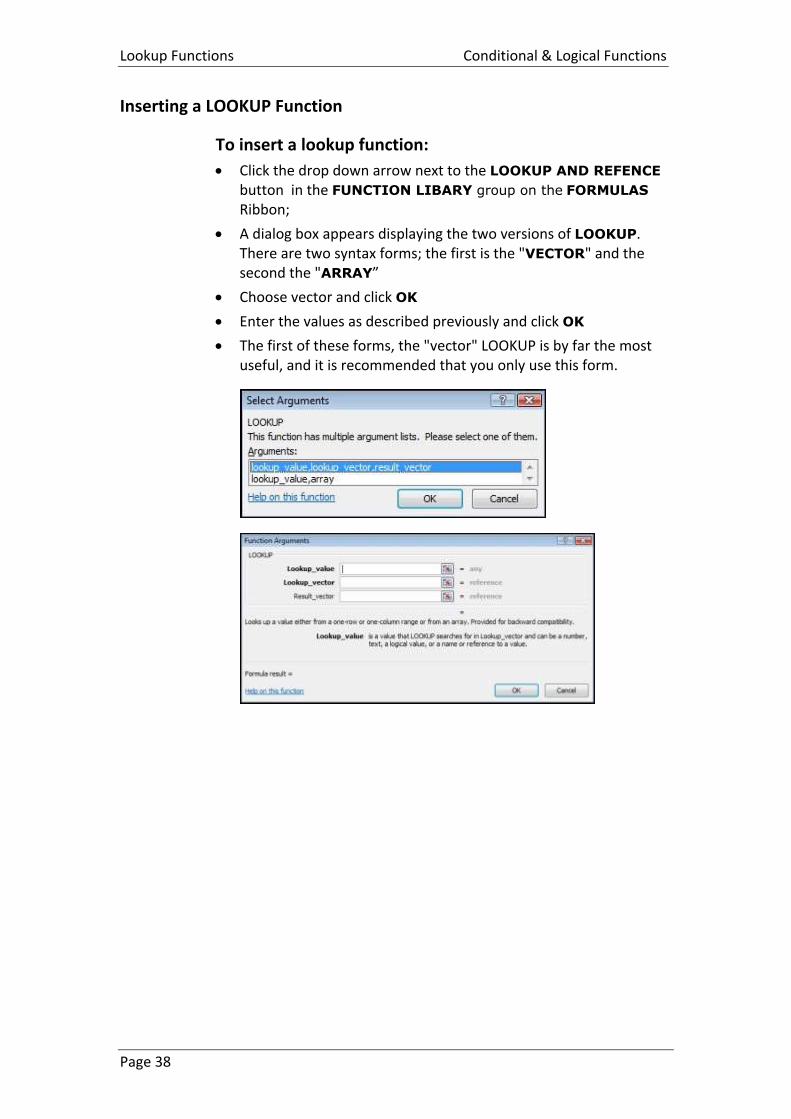
To insert a lookup function:
Click the drop down arrow next to the LOOKUP AND REFENCE
button in the FUNCTION LIBARY group on the FORMULAS Ribbon;
A dialog box appears displaying the two versions of LOOKUP. There are two syntax forms; the first is the "VECTOR" and the second the "ARRAY”
Choose vector and click OK
Enter the values as described previously and click OK
The first of these forms, the "vector" LOOKUP is by far the most useful, and it is recommended that you only use this form.
Excel Formulas and Functions.docx Conditional & Logical Functions
Page 39
Hlookup
The horizontal LOOKUP function (HLOOKUP) can be used not just on a "VECTOR" (single column or row of data), but on an "array" (multiple rows and columns). HLOOKUP searches for a specified value horizontally along the top row of an array. When the value is found, HLOOKUP searches down to a specified row and enters the value of the cell. This is useful when data is arranged in a large tabular format, and it would be difficult for you to read across columns and then down to the appropriate cell. HLOOKUP will do this automatically.
The syntax for HLOOKUP is;
=HLOOKUP( lookup_value , table_array , row_index_number)
The LOOKUP_VALUE is, as before, a number, text string or cell reference which is the value to be found along the top row of the data; the TABLE_ARRAY is the cell references (or range name) of the entire table of data; the ROW_INDEX_NUMBER represents the row from which the result is required. This must be a number, e.g. 4 instructs HLOOKUP to extract a value from row 4 of the TABLE_ARRAY.
It is important to remember that data in the array must be in ascending order. With a simple LOOKUP function, only one column or row of data, referred to as a vector, is required. HLOOKUP uses an array (i.e. more than one column or row of data). Therefore, as HLOOKUP searches horizontally (i.e. across the array), data in the first row must be in ascending order, i.e. numbers from lowest to highest, text from A to Z. As with LOOKUP, if this rule is ignored, HLOOKUP will return the wrong value.
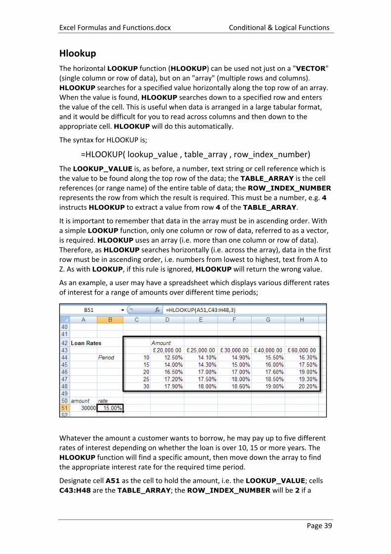
As an example, a user may have a spreadsheet which displays various different rates of interest for a range of amounts over different time periods;
Whatever the amount a customer wants to borrow, he may pay up to five different rates of interest depending on whether the loan is over 10, 15 or more years. The HLOOKUP function will find a specific amount, then move down the array to find the appropriate interest rate for the required time period.
Designate cell A51 as the cell to hold the amount, i.e. the LOOKUP_VALUE; cells C43:H48 are the TABLE_ARRAY; the ROW_INDEX_NUMBER will be 2 if a
Lookup Functions Conditional & Logical Functions
Page 40
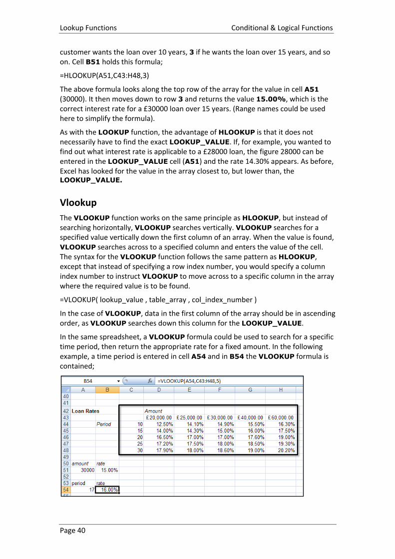
customer wants the loan over 10 years, 3 if he wants the loan over 15 years, and so on. Cell B51 holds this formula;
=HLOOKUP(A51,C43:H48,3)
The above formula looks along the top row of the array for the value in cell A51 (30000). It then moves down to row 3 and returns the value 15.00%, which is the correct interest rate for a £30000 loan over 15 years. (Range names could be used here to simplify the formula).
As with the LOOKUP function, the advantage of HLOOKUP is that it does not necessarily have to find the exact LOOKUP_VALUE. If, for example, you wanted to find out what interest rate is applicable to a £28000 loan, the figure 28000 can be entered in the LOOKUP_VALUE cell (A51) and the rate 14.30% appears. As before, Excel has looked for the value in the array closest to, but lower than, the LOOKUP_VALUE.
Vlookup
The VLOOKUP function works on the same principle as HLOOKUP, but instead of searching horizontally, VLOOKUP searches vertically. VLOOKUP searches for a specified value vertically down the first column of an array. When the value is found, VLOOKUP searches across to a specified column and enters the value of the cell. The syntax for the VLOOKUP function follows the same pattern as HLOOKUP, except that instead of specifying a row index number, you would specify a column index number to instruct VLOOKUP to move across to a specific column in the array where the required value is to be found.
=VLOOKUP( lookup_value , table_array , col_index_number )
In the case of VLOOKUP, data in the first column of the array should be in ascending order, as VLOOKUP searches down this column for the LOOKUP_VALUE.
In the same spreadsheet, a VLOOKUP formula could be used to search for a specific time period, then return the appropriate rate for a fixed amount. In the following example, a time period is entered in cell A54 and in B54 the VLOOKUP formula is contained;
Excel Formulas and Functions.docx Conditional & Logical Functions
Page 41
Cell B54 holds this formula;
=VLOOKUP(A54,C43:H48,5)
The cell A54 is the LOOKUP_VALUE (time period), the TABLE_ARRAY is as before, and for this example rates are looked up for a loan of £40000, hence the COLUMN_INDEX_NUMBER 5. By changing the value of cell A54, the appropriate rate for that time period is returned. Where the specific lookup_value is not found, VLOOKUP works in the same way as HLOOKUP. In other words, the nearest value in the array that is less than the LOOKUP_VALUE will be returned. So, a £40000 loan over 17 years would return an interest rate of 16.00%.
Nested Lookups
One of the limitations of the horizontal and vertical LOOKUP functions is that for every LOOKUP_VALUE changed, the column or row index number stays constant. Using our example, the HLOOKUP will search for any amount, but always for the same time period. Conversely, the VLOOKUP will search for any time period, but always for the same amount. In both cases, if you want to alter the time period and the amount the formula must be edited to alter the column or row index number.
There is, however, a technique whereby one LOOKUP function is "nested" within another. This looks up one value, which will then be used in a second LOOKUP formula as a column or row index number. Using this technique allows you to, say, enter a time period and an amount and see the correct interest rate.
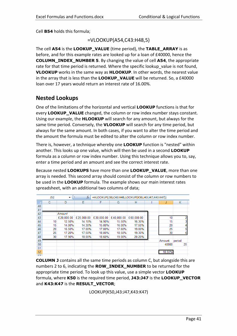
Because nested LOOKUPS have more than one LOOKUP_VALUE, more than one array is needed. This second array should consist of the column or row numbers to be used in the LOOKUP formula. The example shows our main interest rates spreadsheet, with an additional two columns of data;
COLUMN J contains all the same time periods as column C, but alongside this are numbers 2 to 6, indicating the ROW_INDEX_NUMBER to be returned for the appropriate time period. To look up this value, use a simple vector LOOKUP formula, where K50 is the required time period, J43:J47 is the LOOKUP_VECTOR and K43:K47 is the RESULT_VECTOR;
LOOKUP(K50,J43:J47,K43:K47)
Lookup Functions Conditional & Logical Functions
Page 42
Notice there is no equals sign, because this formula is not being entered in a cell of its own. The formula will return a value between 2 and 6 which will be used as a ROW_INDEX_NUMBER in a HLOOKUP formula. This HLOOKUP will look in the main interest rate table for an amount typed in by you, and will respond to the ROW_INDEX_NUMBER returned from the nested LOOKUP formula. The cells J50 and K50 hold the amount and time period to be typed in by you, and the entire nested HLOOKUP, typed in J52, is as follows;
=HLOOKUP(J50,C43:H48,LOOKUP(K50,J43:J47,K43:K47))
In the example, the time period 25 is vertically looked up in COLUMN J and the corresponding value 5 is returned. Also, the amount 40000 is horizontally looked up in the main table, with a ROW_INDEX_NUMBER of 5. The end result is an interest rate of 18.50%. Simply by changing cells J50 and K50, the correct interest rate is always returned for the amount and period typed in.
MATCH()
This function can be used to find out the position of a value in an array. If it matches the first value the function returns a result of 1, the second value returns 2 and so on.
=MATCH(lookup_value, lookup_array, match_type)
lookup_value A value that MATCH() searches for in the lookup_array.
lookup_array A range of cells containing text, numbers or formulae.
match_type 1 the values in the lookup_array must be in ascending order.
0 the values can be in any order, as the function must find an exact match.
-1 the values must be in descending order.
The MATCH() function is unlikely to be used on its own. It can be intelligently used as a substitute for the col_index_num or row_index_num argument in either the VLOOKUP() or HLOOKUP() functions. See the next example.
Two-Way Lookup
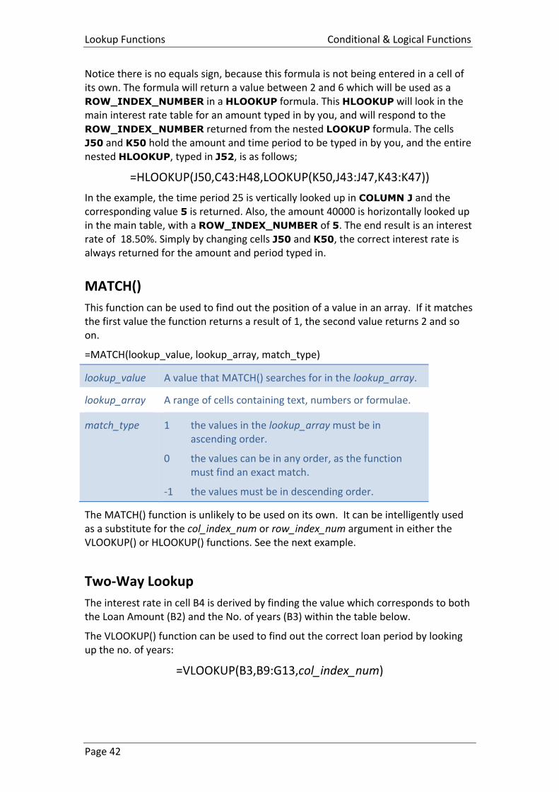
The interest rate in cell B4 is derived by finding the value which corresponds to both the Loan Amount (B2) and the No. of years (B3) within the table below.
The VLOOKUP() function can be used to find out the correct loan period by looking up the no. of years:
=VLOOKUP(B3,B9:G13,col_index_num)
Excel Formulas and Functions.docx Conditional & Logical Functions
Page 43
However the function requires a value for the col_index_num. This should be the column number which is appropriate for the loan amount, for example £25,000 is the third column in the table which means the col_index_num would need to be 3.
Rather than manually inputting the col_index_num, it can be automatically worked out by using the MATCH() function:
=MATCH(B2,B8:G8,1) This function will return the value 4.
The VLOOKUP() and MATCH() functions can be combined to find the correct interest rate:
=VLOOKUP(B3,B9:G13,MATCH(B2,B8:G8,1))
INDEX Function
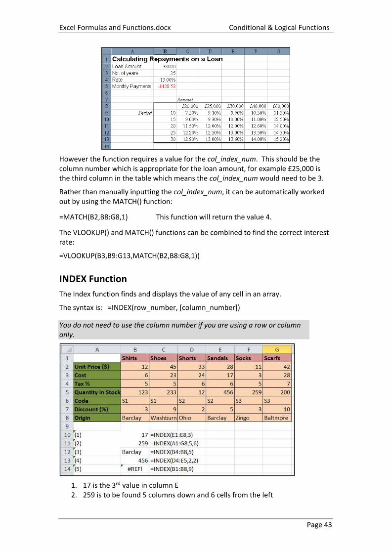
The Index function finds and displays the value of any cell in an array.
The syntax is: =INDEX(row_number, [column_number])
You do not need to use the column number if you are using a row or column only.
1. 17 is the 3rd value in column E 2. 259 is to be found 5 columns down and 6 cells from the left
Lookup Functions Conditional & Logical Functions
Page 44
3. Barclay is the value of the 5th cell from top in the array B4:B8 4. 456 is the value of the cell 2nd from top and 3nd from left in the array D4:E5 5. #REF is the error Excel gives because there is no value in the 9th cell in the
array B1:B8
Combining MATCH and INDEX
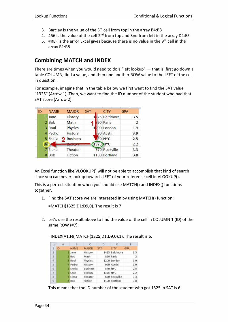
There are times when you would need to do a “left lookup” — that is, first go down a table COLUMN, find a value, and then find another ROW value to the LEFT of the cell in question.
For example, imagine that in the table below we first want to find the SAT value “1325″ (Arrow 1). Then, we want to find the ID number of the student who had that SAT score (Arrow 2):
An Excel function like VLOOKUP() will not be able to accomplish that kind of search since you can never lookup towards LEFT of your reference cell in VLOOKUP().
This is a perfect situation when you should use MATCH() and INDEX() functions together.
1. Find the SAT score we are interested in by using MATCH() function:
=MATCH(1325,D1:D9,0). The result is 7
2. Let’s use the result above to find the value of the cell in COLUMN 1 (ID) of the same ROW (#7): =INDEX(A1:F9,MATCH(1325,D1:D9,0),1). The result is 6.
This means that the ID number of the student who got 1325 in SAT is 6.
Excel Formulas and Functions.docx Conditional & Logical Functions
Page 45
Choose
The Choose function uses an index number to return a value from the list of arguments. Use CHOOSE to select one of up to 29 values based on the index number. For example, if value 1 through value 7 are the days of the week, CHOOSE returns one of the days when a number between 1 and 7 is used as index_num.
Syntax
CHOOSE(index_num, value1, value2,…)
Index_num specifies which value argument is selected. Index_num must be a number between 1 and 29, or a formula or reference to a cell containing a number between 1 and 29.
Value1, Value2,… are 1 to 29 value arguments from which CHOOSE selects a value or an action to perform based on index_num. The arguments can be numbers, cell references, defined names, formulas, functions or text.
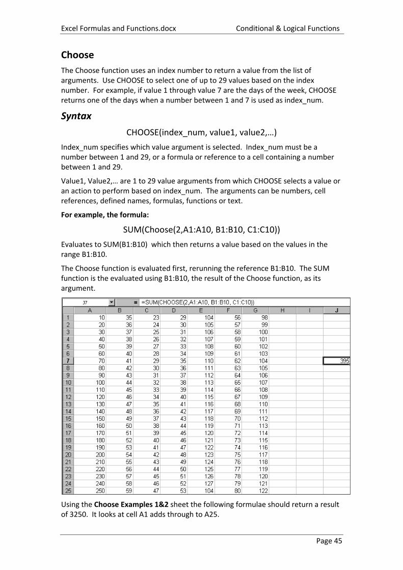
For example, the formula:
SUM(Choose(2,A1:A10, B1:B10, C1:C10))
Evaluates to SUM(B1:B10) which then returns a value based on the values in the range B1:B10.
The Choose function is evaluated first, rerunning the reference B1:B10. The SUM function is the evaluated using B1:B10, the result of the Choose function, as its argument.
Using the Choose Examples 1&2 sheet the following formulae should return a result of 3250. It looks at cell A1 adds through to A25.
Lookup Functions Conditional & Logical Functions
Page 46
SUM(A1:CHOOSE(3,A10,A20, A25))
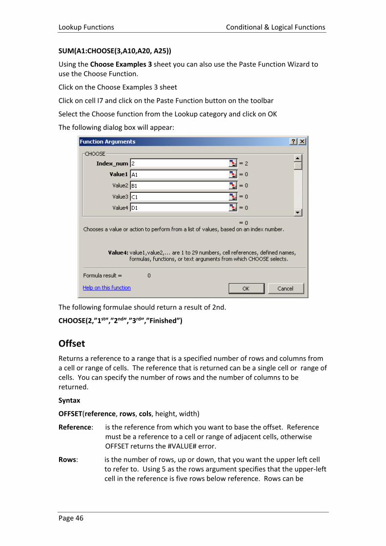
Using the Choose Examples 3 sheet you can also use the Paste Function Wizard to use the Choose Function.
Click on the Choose Examples 3 sheet
Click on cell I7 and click on the Paste Function button on the toolbar
Select the Choose function from the Lookup category and click on OK
The following dialog box will appear:
The following formulae should return a result of 2nd.
CHOOSE(2,”1st”,”2nd”,”3rd”,”Finished”)
Offset
Returns a reference to a range that is a specified number of rows and columns from a cell or range of cells. The reference that is returned can be a single cell or range of cells. You can specify the number of rows and the number of columns to be returned.
Syntax
OFFSET(reference, rows, cols, height, width)
Reference: is the reference from which you want to base the offset. Reference must be a reference to a cell or range of adjacent cells, otherwise OFFSET returns the #VALUE# error.
Rows: is the number of rows, up or down, that you want the upper left cell to refer to. Using 5 as the rows argument specifies that the upper-left cell in the reference is five rows below reference. Rows can be
Excel Formulas and Functions.docx Conditional & Logical Functions
Page 47
positive, which means below the starting reference) or negative, which means above the starting reference.
Columns: is the number of columns to the left or right that you want the upper left cell of the result to refer to. Using 5 as the cols argument specifies that the upper left cell in the reference is 5 columns to the right of the reference. Columns can be positive, which means to the right of the starting reference, or negative, which means to the left of the starting reference.
If the rows or columns offset reference goes over the edge of the worksheet OFFSET returns the #REF# error value.
OFFSET does not actually move any cells or change the selection, it merely returns a reference. OFFSET can be used with any function expecting a reference argument.
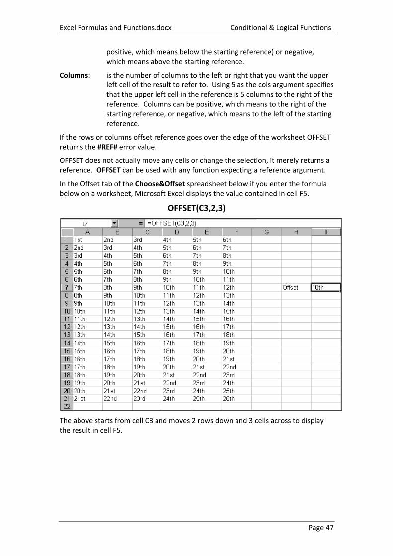
In the Offset tab of the Choose&Offset spreadsheet below if you enter the formula below on a worksheet, Microsoft Excel displays the value contained in cell F5.
OFFSET(C3,2,3)
The above starts from cell C3 and moves 2 rows down and 3 cells across to display the result in cell F5.
Lookup Functions Financial Functions
Page 48
Financial Functions
NPV()
Most business enterprises and investors are required to decide whether a particular business venture or investment is worthwhile and should proceed. In many cases, a comparison between alternative projects is also required. That is, a financial assessment of each proposal is necessary before it commences so that the appropriate decision is made. The NPV() function, Net Present Value, can be used as a basis for this type of decision.
NPV() returns the net present value of an investment based on a series of periodic cash flows and a discount rate. The net present value of an investment is today's value of a series of future payments (negative values) and income (positive values).
=NPV(rate,value1,value2,value3,...)
rate This is a percentage rate, which might represent the rate of inflation or the interest rate of a competing investment.
value1 This can be a single value representing either payment or income at the end of the first period. The rest of the cash flows can be entered as value2, value3 etc. (up to 29).
Alternatively, it can be a range of cells containing cash flows where the first value occurs at the end of the first period.
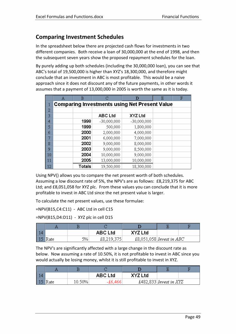
Excel Formulas and Functions.docx Financial Functions
Page 49
Comparing Investment Schedules
In the spreadsheet below there are projected cash flows for investments in two different companies. Both receive a loan of 30,000,000 at the end of 1998, and then the subsequent seven years show the proposed repayment schedules for the loan.
By purely adding up both schedules (including the 30,000,000 loan), you can see that ABC's total of 19,500,000 is higher than XYZ's 18,300,000, and therefore might conclude that an investment in ABC is most profitable. This would be a naive approach since it does not discount any of the future payments, in other words it assumes that a payment of 13,000,000 in 2005 is worth the same as it is today.
Using NPV() allows you to compare the net present worth of both schedules. Assuming a low discount rate of 5%, the NPV's are as follows: £8,219,375 for ABC Ltd; and £8,051,058 for XYZ plc. From these values you can conclude that it is more profitable to invest in ABC Ltd since the net present value is larger.
To calculate the net present values, use these formulae:
=NPV(B15,C4:C11) - ABC Ltd in cell C15
=NPV(B15,D4:D11) - XYZ plc in cell D15
The NPV's are significantly affected with a large change in the discount rate as below. Now assuming a rate of 10.50%, it is not profitable to invest in ABC since you would actually be losing money, whilst it is still profitable to invest in XYZ.
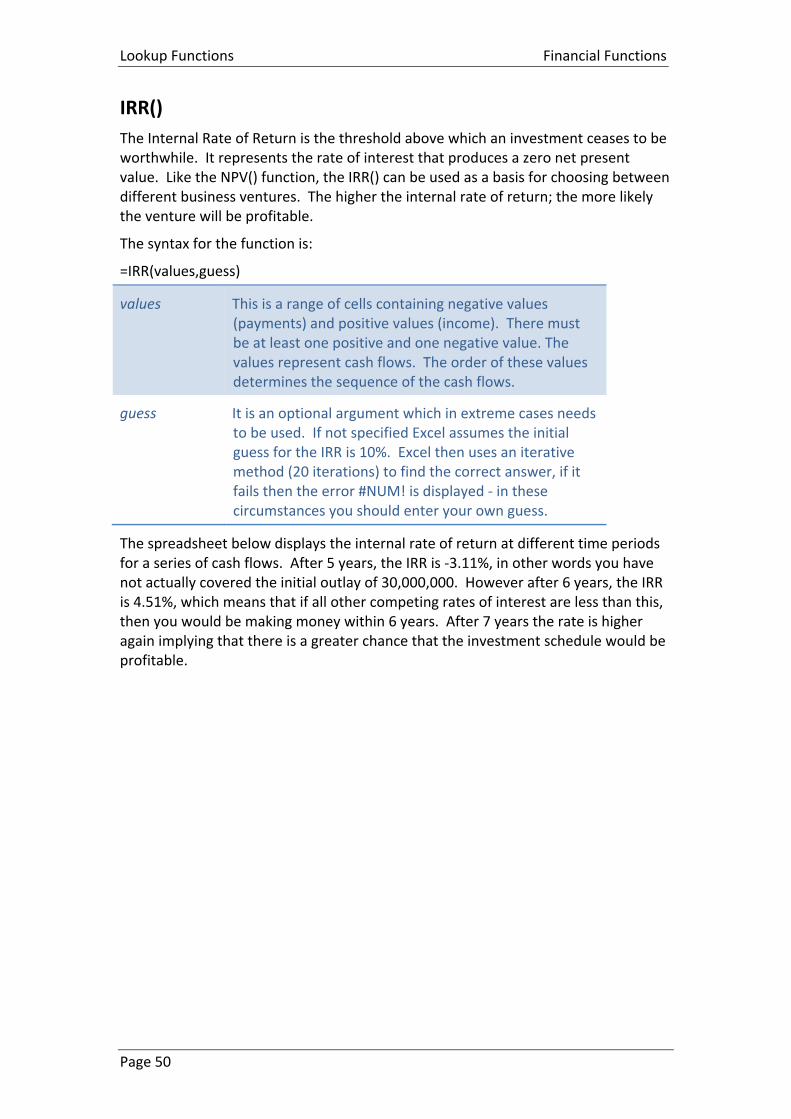
Lookup Functions Financial Functions
Page 50
IRR()
The Internal Rate of Return is the threshold above which an investment ceases to be worthwhile. It represents the rate of interest that produces a zero net present value. Like the NPV() function, the IRR() can be used as a basis for choosing between different business ventures. The higher the internal rate of return; the more likely the venture will be profitable.
The syntax for the function is:
=IRR(values,guess)
values This is a range of cells containing negative values (payments) and positive values (income). There must be at least one positive and one negative value. The values represent cash flows. The order of these values determines the sequence of the cash flows.
guess It is an optional argument which in extreme cases needs to be used. If not specified Excel assumes the initial guess for the IRR is 10%. Excel then uses an iterative method (20 iterations) to find the correct answer, if it fails then the error #NUM! is displayed - in these circumstances you should enter your own guess.
The spreadsheet below displays the internal rate of return at different time periods for a series of cash flows. After 5 years, the IRR is -3.11%, in other words you have not actually covered the initial outlay of 30,000,000. However after 6 years, the IRR is 4.51%, which means that if all other competing rates of interest are less than this, then you would be making money within 6 years. After 7 years the rate is higher again implying that there is a greater chance that the investment schedule would be profitable.
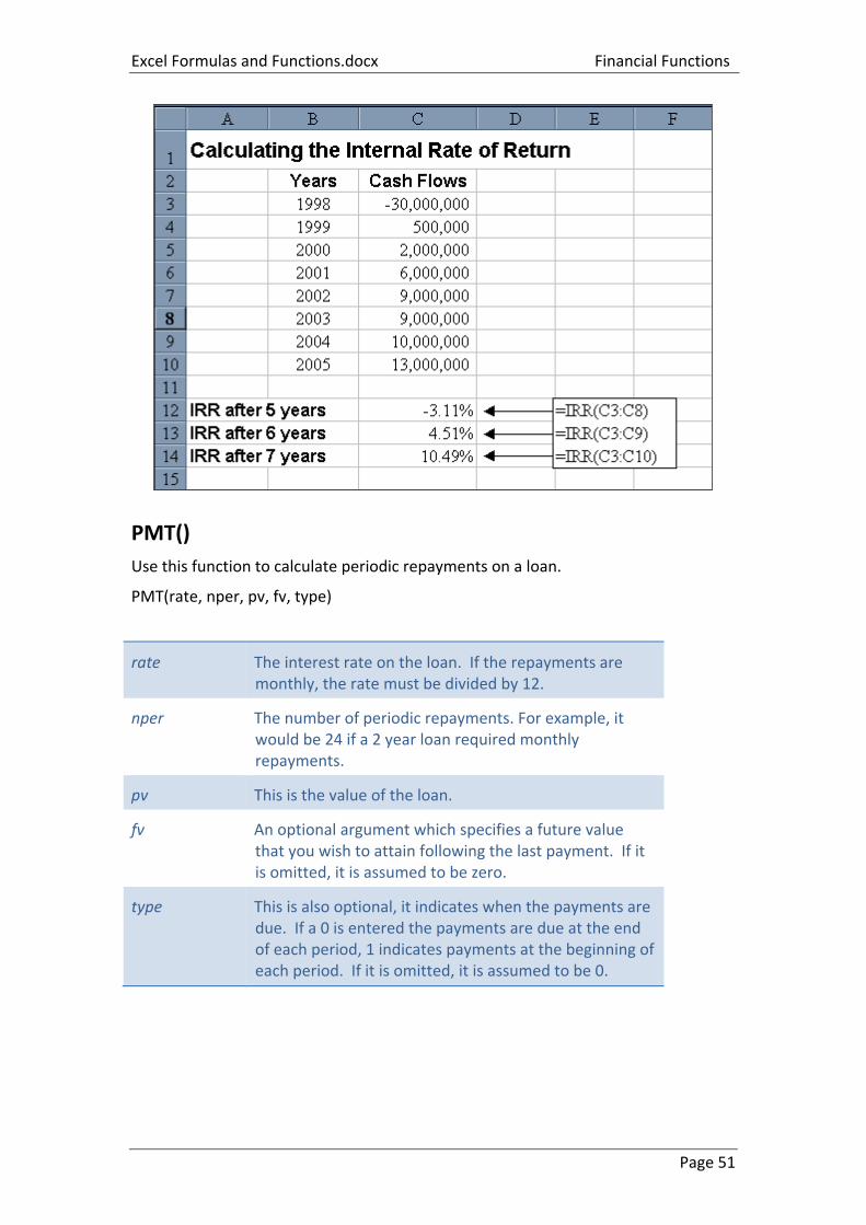
Excel Formulas and Functions.docx Financial Functions
Page 51
PMT()
Use this function to calculate periodic repayments on a loan.
PMT(rate, nper, pv, fv, type)
rate The interest rate on the loan. If the repayments are monthly, the rate must be divided by 12.
nper The number of periodic repayments. For example, it would be 24 if a 2 year loan required monthly repayments.
pv This is the value of the loan.
fv An optional argument which specifies a future value that you wish to attain following the last payment. If it is omitted, it is assumed to be zero.
type This is also optional, it indicates when the payments are due. If a 0 is entered the payments are due at the end of each period, 1 indicates payments at the beginning of each period. If it is omitted, it is assumed to be 0.
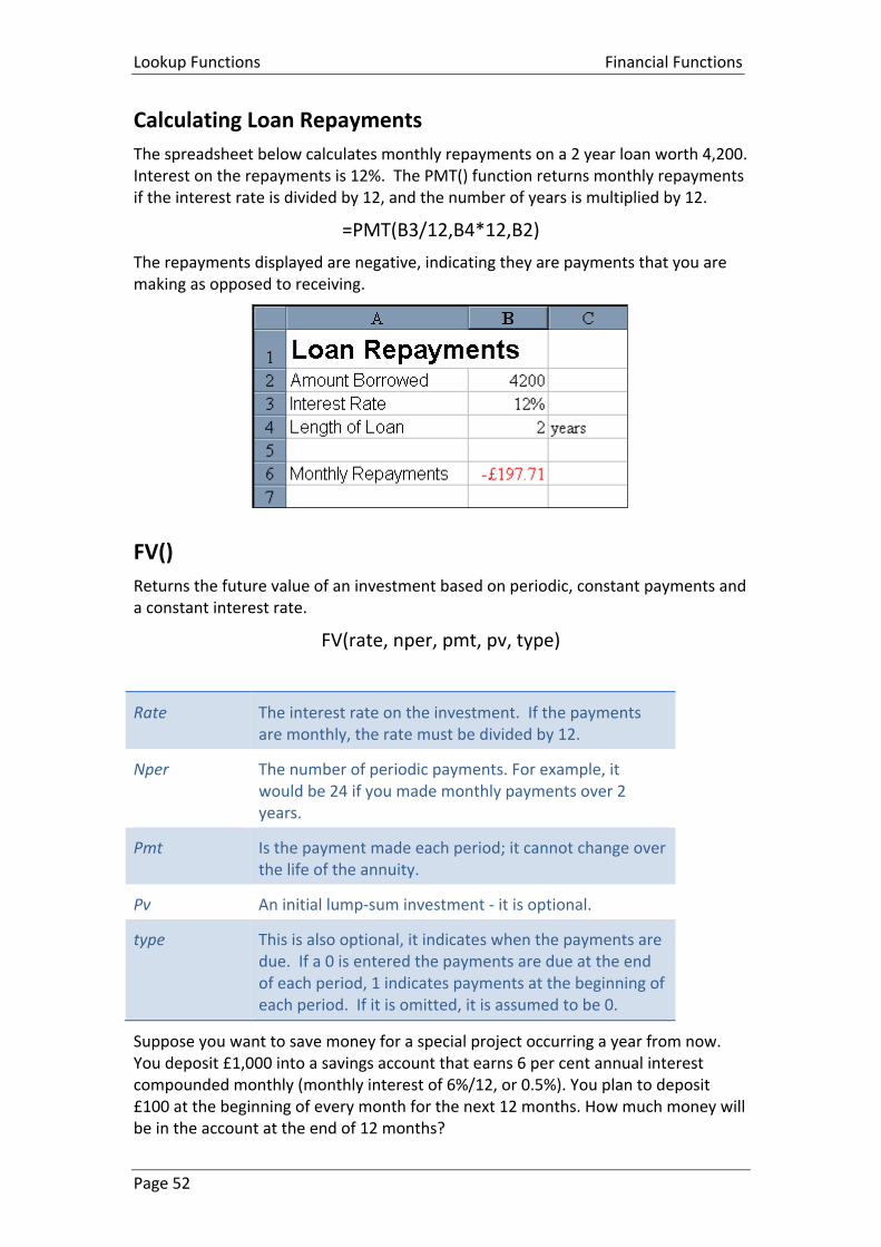
Lookup Functions Financial Functions
Page 52
Calculating Loan Repayments
The spreadsheet below calculates monthly repayments on a 2 year loan worth 4,200. Interest on the repayments is 12%. The PMT() function returns monthly repayments if the interest rate is divided by 12, and the number of years is multiplied by 12.
=PMT(B3/12,B4*12,B2)
The repayments displayed are negative, indicating they are payments that you are making as opposed to receiving.
FV()
Returns the future value of an investment based on periodic, constant payments and a constant interest rate.
FV(rate, nper, pmt, pv, type)
Rate The interest rate on the investment. If the payments are monthly, the rate must be divided by 12.
Nper The number of periodic payments. For example, it would be 24 if you made monthly payments over 2 years.
Pmt Is the payment made each period; it cannot change over the life of the annuity.
Pv An initial lump-sum investment - it is optional.
type This is also optional, it indicates when the payments are due. If a 0 is entered the payments are due at the end of each period, 1 indicates payments at the beginning of each period. If it is omitted, it is assumed to be 0.
Suppose you want to save money for a special project occurring a year from now. You deposit £1,000 into a savings account that earns 6 per cent annual interest compounded monthly (monthly interest of 6%/12, or 0.5%). You plan to deposit £100 at the beginning of every month for the next 12 months. How much money will be in the account at the end of 12 months?
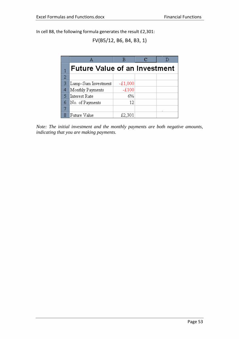
Excel Formulas and Functions.docx Financial Functions
Page 53
In cell B8, the following formula generates the result £2,301:
FV(B5/12, B6, B4, B3, 1)
Note: The initial investment and the monthly payments are both negative amounts,
indicating that you are making payments.
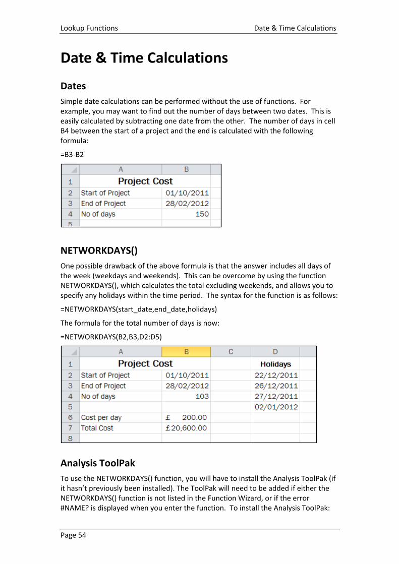
Lookup Functions Date & Time Calculations
Page 54
Date & Time Calculations
Dates
Simple date calculations can be performed without the use of functions. For example, you may want to find out the number of days between two dates. This is easily calculated by subtracting one date from the other. The number of days in cell B4 between the start of a project and the end is calculated with the following formula:
=B3-B2
NETWORKDAYS()
One possible drawback of the above formula is that the answer includes all days of the week (weekdays and weekends). This can be overcome by using the function NETWORKDAYS(), which calculates the total excluding weekends, and allows you to specify any holidays within the time period. The syntax for the function is as follows:
=NETWORKDAYS(start_date,end_date,holidays)
The formula for the total number of days is now:
=NETWORKDAYS(B2,B3,D2:D5)
Analysis ToolPak
To use the NETWORKDAYS() function, you will have to install the Analysis ToolPak (if it hasn’t previously been installed). The ToolPak will need to be added if either the NETWORKDAYS() function is not listed in the Function Wizard, or if the error #NAME? is displayed when you enter the function. To install the Analysis ToolPak:
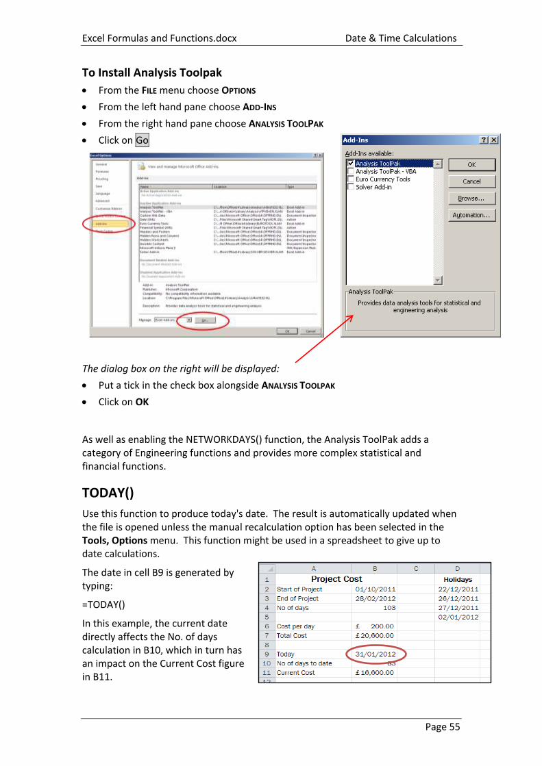
Excel Formulas and Functions.docx Date & Time Calculations
Page 55
To Install Analysis Toolpak
From the FILE menu choose OPTIONS
From the left hand pane choose ADD-INS
From the right hand pane choose ANALYSIS TOOLPAK
Click on Go
The dialog box on the right will be displayed:
Put a tick in the check box alongside ANALYSIS TOOLPAK
Click on OK
As well as enabling the NETWORKDAYS() function, the Analysis ToolPak adds a category of Engineering functions and provides more complex statistical and financial functions.
TODAY()
Use this function to produce today's date. The result is automatically updated when the file is opened unless the manual recalculation option has been selected in the Tools, Options menu. This function might be used in a spreadsheet to give up to date calculations.
The date in cell B9 is generated by typing:
=TODAY()
In this example, the current date directly affects the No. of days calculation in B10, which in turn has an impact on the Current Cost figure in B11.
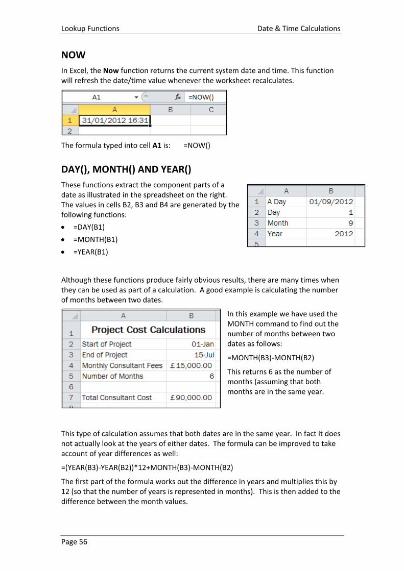
Lookup Functions Date & Time Calculations
Page 56
NOW
In Excel, the Now function returns the current system date and time. This function will refresh the date/time value whenever the worksheet recalculates.
The formula typed into cell A1 is: =NOW()
DAY(), MONTH() AND YEAR()
These functions extract the component parts of a date as illustrated in the spreadsheet on the right. The values in cells B2, B3 and B4 are generated by the following functions:
=DAY(B1)
=MONTH(B1)
=YEAR(B1)
Although these functions produce fairly obvious results, there are many times when they can be used as part of a calculation. A good example is calculating the number of months between two dates.
In this example we have used the MONTH command to find out the number of months between two dates as follows:
=MONTH(B3)-MONTH(B2)
This returns 6 as the number of months (assuming that both months are in the same year.
This type of calculation assumes that both dates are in the same year. In fact it does not actually look at the years of either dates. The formula can be improved to take account of year differences as well:
=(YEAR(B3)-YEAR(B2))*12+MONTH(B3)-MONTH(B2)
The first part of the formula works out the difference in years and multiplies this by 12 (so that the number of years is represented in months). This is then added to the difference between the month values.
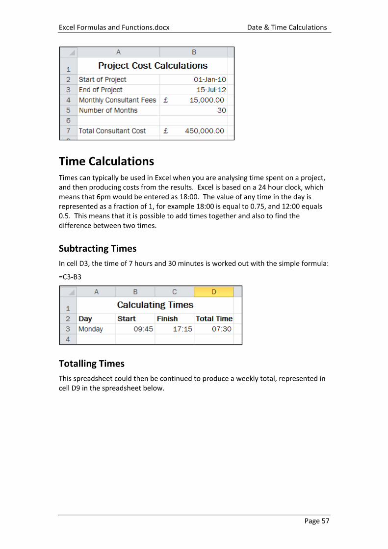
Excel Formulas and Functions.docx Date & Time Calculations
Page 57
Time Calculations Times can typically be used in Excel when you are analysing time spent on a project, and then producing costs from the results. Excel is based on a 24 hour clock, which means that 6pm would be entered as 18:00. The value of any time in the day is represented as a fraction of 1, for example 18:00 is equal to 0.75, and 12:00 equals 0.5. This means that it is possible to add times together and also to find the difference between two times.
Subtracting Times
In cell D3, the time of 7 hours and 30 minutes is worked out with the simple formula:
=C3-B3
Totalling Times
This spreadsheet could then be continued to produce a weekly total, represented in cell D9 in the spreadsheet below.
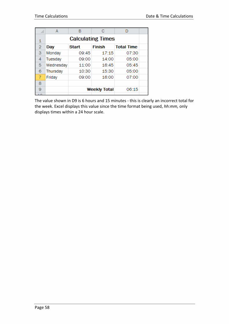
Time Calculations Date & Time Calculations
Page 58
The value shown in D9 is 6 hours and 15 minutes - this is clearly an incorrect total for the week. Excel displays this value since the time format being used, hh:mm, only displays times within a 24 hour scale.
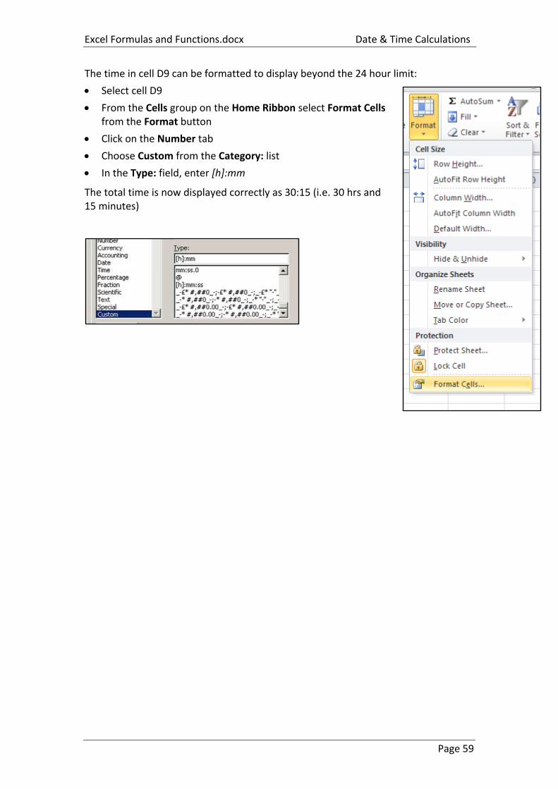
Excel Formulas and Functions.docx Date & Time Calculations
Page 59
The time in cell D9 can be formatted to display beyond the 24 hour limit:
Select cell D9
From the Cells group on the Home Ribbon select Format Cells from the Format button
Click on the Number tab
Choose Custom from the Category: list
In the Type: field, enter [h]:mm
The total time is now displayed correctly as 30:15 (i.e. 30 hrs and 15 minutes)
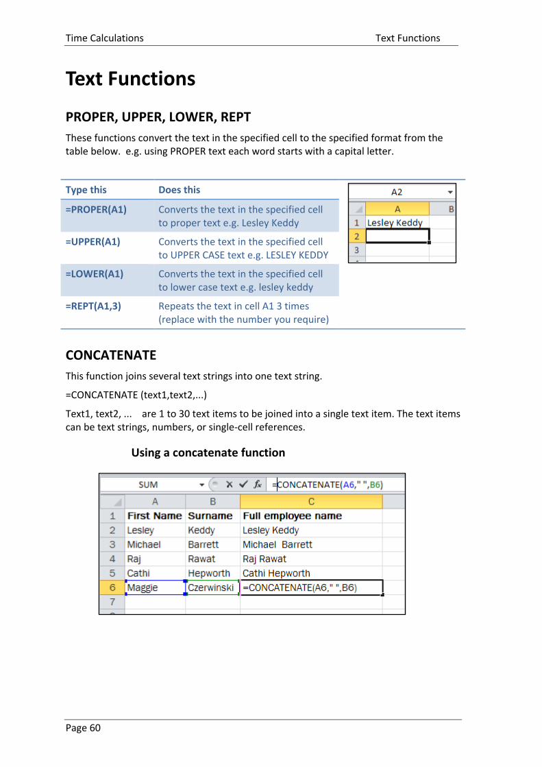
Time Calculations Text Functions
Page 60
Text Functions
PROPER, UPPER, LOWER, REPT
These functions convert the text in the specified cell to the specified format from the table below. e.g. using PROPER text each word starts with a capital letter.
Type this Does this
=PROPER(A1) Converts the text in the specified cell to proper text e.g. Lesley Keddy
=UPPER(A1) Converts the text in the specified cell to UPPER CASE text e.g. LESLEY KEDDY
=LOWER(A1) Converts the text in the specified cell to lower case text e.g. lesley keddy
=REPT(A1,3) Repeats the text in cell A1 3 times (replace with the number you require)
CONCATENATE
This function joins several text strings into one text string.
=CONCATENATE (text1,text2,...)
Text1, text2, ... are 1 to 30 text items to be joined into a single text item. The text items can be text strings, numbers, or single-cell references.
Using a concatenate function
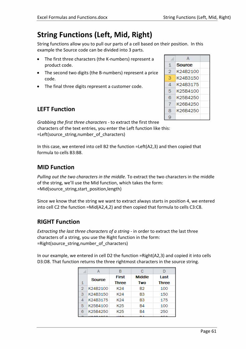
Excel Formulas and Functions.docx String Functions (Left, Mid, Right)
Page 61
String Functions (Left, Mid, Right) String functions allow you to pull our parts of a cell based on their position. In this example the Source code can be divided into 3 parts.
The first three characters (the K-numbers) represent a product code.
The second two digits (the B-numbers) represent a price code.
The final three digits represent a customer code.
LEFT Function Grabbing the first three characters - to extract the first three characters of the text entries, you enter the Left function like this: =Left(source_string,number_of_characters) In this case, we entered into cell B2 the function =Left(A2,3) and then copied that formula to cells B3:B8.
MID Function
Pulling out the two characters in the middle. To extract the two characters in the middle of the string, we’ll use the Mid function, which takes the form: =Mid(source_string,start_position,length) Since we know that the string we want to extract always starts in position 4, we entered into cell C2 the function =Mid(A2,4,2) and then copied that formula to cells C3:C8.
RIGHT Function
Extracting the last three characters of a string - in order to extract the last three characters of a string, you use the Right function in the form: =Right(source_string,number_of_characters) In our example, we entered in cell D2 the function =Right(A2,3) and copied it into cells D3:D8. That function returns the three rightmost characters in the source string.


![[XLS]faculty.fuqua.duke.edupecklund/ExcelReview/... · Web viewCharting Data Tables Formulas Basic Editing Formatting Naming Ranges Introduction cement Interest_rate Principal SALES](https://img.pdfslide.us/doc/110x75/5b1fc4777f8b9a20508b5601/xls-pecklundexcelreview-web-viewcharting-data-tables-formulas-basic-editing.jpg)