Embed Size (px)
Citation preview
MS-EXCEL STATISTICAL PROCEDURES
Cini Varghese
Indian Agricultural Statistics Research Institute
Library Avenue New Delhi ndash 110012
cini_viasriresin
Microsoft (MS) Excel ( ) is a powerful spreadsheet that is easy to use and allows you to
store manipulate analyze and visualize data It also supports databases graphic and
presentation features It is a powerful research tool and needs a minimum of teaching
Spreadsheets offer the potential to bring the real numerical work alive and make statistics
enjoyable But the main disadvantage is that some advanced statistical functions are not
available and it takes a longer computing time as compared to other specialized softwares
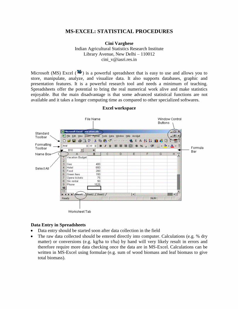
Excel workspace
Data Entry in Spreadsheets
Data entry should be started soon after data collection in the field
The raw data collected should be entered directly into computer Calculations (eg dry
matter) or conversions (eg kgha to tha) by hand will very likely result in errors and
therefore require more data checking once the data are in MS-Excel Calculations can be
written in MS-Excel using formulae (eg sum of wood biomass and leaf biomass to give
total biomass)
M I 2 MS-EXCEL Statistical Procedures
M I-31
Data Checking
One can use calculations and conversions for data checking For example if the collected data
is grain yield per plot it may be difficult to see whether the values are reasonable However if
these are converted to yield per hectare then one can compare the numbers with our scientific
knowledge of grain yields Simple formulae can be written to check for consistency in the
data For example if tree height is measured 3 times in the year a simple formula that
subtracts tree height 1 from tree height 2can be used to check the correctness of the
data The numbers in the resulting column should all be positive We cannot have a shrinking
tree For new columns of calculated or converted data suitable header information (what the
new column is units and short name) at the top of the data should be included
Missing Values
In MS-Excel the missing values are BLANK cells It is useful to know this when calculating
formulae and summaries of the data For example when calculating the average of a number
of cells if one cell is blank MS-Excel ignores this as an observation (ie the average is the
sumnumber of non-blank cells) But if the cell contains a 0 then this is included in the
calculation (ie the average is the sumno of cells) In a column of number of fruit per plot
a missing value could signify zero (tree is there but no fruit) dead (tree was there but died so
no fruit) lost (measurement was lost illegible) or not representative (tree had been browsed
severely by goats) In this example depending on the objectives of the trial the scientist
might choose to put a 0 in the cells of trees with no fruit and leave blank (but add comments)
for the other missing values
Pivot Tables (to check consistency between replicates)
Variation between replicates is expected but some level of consistency is also usual We can
use pivot tables to look at the data A pivot table is an interactive worksheet table that quickly
summarizes large amount of data using a format and calculation methods you choose It is
called pivot table because you can rotate its row and column heading around the core data
area to give you different views of the source data A pivot table provides an easy way for you
to display and analyze summary information about data already created in MS-Excel or other
application
Scatter Plots (to check consistency between variates)
We can often expect two measured variables to have a fairly consistent relationship with each
other For example number of fruits with weight of fruits or Stover yield plotted against
grain yield To look for odd values we could plot one against the other in a scatter
plot Scatter plots are useful tools for helping to spot outliers
Line Plots (to examine changes over time)
Where measurements on a unit are taken on several occasions over a period of time it may be
possible to check that the changes are realistic A check back at the problematic data which is
not in the usual trend can be made
Double Data Entry One effective although not always practical way of checking for errors caused by data entry
mistakes is double entry The data are entered by two individuals onto separate sheets that
M I 2 MS-EXCEL Statistical Procedures
M I-32
have the same design structure The sheets are then compared and any inconsistencies are
checked with the original data It is assumed that the two data entry operators will not make
the same errors There is no built-in system for double entry in MS-Excel However there
are some functions that can be used to compare the two copies An example is the DELTA
function that compares two values and returns a 1 if they are the same and a 0 otherwise To
use this function we would set up a third worksheet and input a formula into each cell that
compares the two identical cells in the other two worksheets The 0s on the third worksheet
will therefore identify the contradictions between the two sets of data This method can also
be used to check survey data but for the process to work the records must be entered in
exactly the same order in both sheets If a section at the bottom of the third worksheet
contains mostly 0s this could indicate that you have omitted a record in one of the other
sheets
Preparing Data for Export to a Statistical Package Statistical analysis of research data usually involves exporting the data into a statistical
package such as GENSTAT SAS or SPSS These packages require you to give the MS-Excel
cell range from which data are to be taken In the latest editions of MS-Excel we can mark
these ranges within MS-Excel and then transfer them directly into the statistical packages
Highlight the data you require including the column titles (the codes which have been
used to label the factors and variables)
Go to the Name Box an empty white box at the top left of the spreadsheet Click in this
box and type a name for the highlighted range (eg Data) Press Enter
From now on when you want to select your data to export go to the Name Box and
select that name (eg Data) The relevant data will then be highlighted
MS-Excel Help If you get stuck on any aspect of MS-Excel then use the Help facility It contains extensive
topics and by typing in a question you can extract the required information See the picture
below for an example
FEATURES OF MS-EXCEL Analytic Features
The windows interface includes windows pull down menus dialog boxes and mouse
support
M I 2 MS-EXCEL Statistical Procedures
M I-33
Repetitive tasks can be automated with MS-Excel Easy to use macros and user
defined functions
Full featured graphing and charting facilities
Supports on screen databases with querying extracting and sorting functions
Permits the user to add edit delete and find database records
Presentation Features
Individual cells and chart text can be formatted to any font and font size
Variations in font size style and alignment control can be determined
The user can add legends text pattern scaling and symbols to charts
Charts and Graphs
A chart is a graphic representation of worksheet data The dimension of a chart depends upon
the range of the data selected Charts are created on a worksheet or as a separate document
that is saved with an extension XLS MS-Excel automatically scales the axes creates columns
categories and labels the columns Values from worksheet cells or data points are displayed as
bars lines columns pie slices or other shapes in the chart Showing a data in a chart can
make it clearer interesting and easier to understand Charts can also help the user to evaluate
hisher data and make comparisons between different worksheet values
Creating Chart
Select worksheet data
Choose ―Insert ―chart
Select ―chart type
Different chart wizard dialog boxes will appear Define titles legends etc
The final screen of the Chart Wizard will give you the option of saving the graph either as its
own sheet or as a part of the current sheet First give a name to your graph by typing your
name of choice in the first white textbox Finally click on the little white circle to the left of
the line ―As new sheet
Click ―Finish
Sorting and Filtering
MS-Excel makes it easy to organize find and create report from data stored in a list
Sort To organize data in a list alphabetically numerically or chronologically
(i) To sort entire list
Select a single cell in the list
Choose ―data ―sort
(ii) Sorting column from left to right
Choose the ―option button in the sort dialog box
In the sort option dialog box select ―sort left to right
Choose ―OK
Filter To quickly find and work with a subset of your data without moving or sorting it
Choose ―Data ―Filter ―Auto Filter
MS-Excel place a drop down arrow directly on the column labels of the list
M I 2 MS-EXCEL Statistical Procedures
M I-34
Clicking arrow displays a list of all the unique items in the column
STATISTICAL FUNCTIONS
Excellsquos statistical functions are quite powerful In general statistical functions take lists as
arguments rather than single numerical values or text A list could be a group of numbers
separated by commas such as (351121516) or a specified range of cells such as (A1A6)
which is the equivalent of typing out the list (A1A2A3A4A5A6)
The function COUNT(list) counts the number of values in a list ignoring empty or
nonnumeric cells whereas COUNTA(list) counts the number of values in the list that have
any entry at all MIN(list) returns a listlsquos smallest value whereas MAX(list) returns a listlsquos
largest value
The functions AVERAGE(list) MEDIAN(list) MODE(list) STDEV(list) all carry out the
statistical operations you would expect (STDEV stands for standard deviation) when you
pass a list of values as an argument
Create a Formula
Formulas are equations that perform calculations on values in your worksheet A formula
starts with an equal sign (=) For example the following formula multiplies 2 by 3 and then
adds 5 to the result =5+23 The following formulas contain operators and constants
Example formula What it does
=128+345 Adds 128 and 345
=5^2 Squares 5
Click the cell in which you want to enter the formula
Type = (an equal sign)
Enter the formula
Press ENTER
Create a Formula that Contains References or Names A1+23
The following formulas contain relative references and names of other cells The cell that
contains the formula is known as a dependent cell when its value depends on the values in
other cells For example cell B2 is a dependent cell if it contains the formula =C2
Example formula What it does
=C2 Uses the value in the cell C2
=Sheet2B2 Uses the value in cell B2 on Sheet2
=Asset-Liability Subtracts a cell named Liability from a cell named Asset
Click the cell in which the formula enter has to be entered
M I 2 MS-EXCEL Statistical Procedures
M I-35
In the formula bar type = (equal sign)
To create a reference select a cell a range of cells a location in another worksheet or a
location in another workbook One can drag the border of the cell selection to move the
selection or drag the corner of the border to expand the selection
Press ENTER
Create a Formula that Contains a Function =AVERAGE(A1B4)
The following formulas contain functions
Example formula What it does
=SUM(AA) Adds all numbers in column A
=AVERAGE(A1B4) Averages all numbers in the range
Click the cell in which the formula enter has to be entered
To start the formula with the function click ―insert function on the formula bar
Select the function
Enter the arguments When the formula is completed press ENTER
Create a Formula with Nested Functions =IF(AVERAGE(F2F5)gt50 SUM(G2G5)0)
Nested functions use a function as one of the arguments of another function The following
formula sums a set of numbers (G2G5) only if the average of another set of numbers (F2F5)
is greater than 50 Otherwise it returns 0
STATISTICAL ANALYSIS TOOLS
Microsoft Excel provides a set of data analysis tools mdash called the Analysis ToolPak mdash that
one can use to save steps when you develop complex statistical or engineering analyses
Provide the data and parameters for each analysis the tool uses the appropriate statistical or
engineering macro functions and then displays the results in an output table Some tools
generate charts in addition to output tables
Accessing the Data Analysis Tools To access various tools included in the Analysis
ToolPak click ―Data Analysis on the ―Tools menu If the ―Data Analysis command is not
available we need to load the Analysis ToolPak ―add-in program
Correlation
The ―Correlation analysis tool measures the relationship between two data sets that are
scaled to be independent of the unit of measurement It can be used to determine whether two
ranges of data move together mdash that is whether large values of one set are associated with
large values of the other (positive correlation) whether small values of one set are associated
with large values of the other (negative correlation) or whether values in both sets are
unrelated (correlation near zero)
M I 2 MS-EXCEL Statistical Procedures
M I-36
If the experimenter had measured two variables in a group of individuals such as foot-length
and height heshe can calculate how closely the variables are correlated with each other
Select ―Tools ―Data Analysis Scroll down the list select ―Correlation and click OK
A new window will appear where the following information needs to be entered
Input range Highlight the two columns of data that are the paired values for the two
variables The cell range will automatically appear in the box If column headings are
included in this range tick the Labels box
Output range Click in this box then select a region on the worksheet where the user want the
data table displayed It can be done by clicking on a single cell which will become the top left
cell of the table
Click OK and a table will be displayed showing the correlation coefficient (r) for the data
CORREL(array1 array2) also returns the correlation coefficient between two data sets
Covariance
Covariance is a measure of the relationship between two ranges of data The ―covariance tool
can be used to determine whether two ranges of data move together ie whether large values
of one set are associated with large values of the other (positive covariance) whether small
values of one set are associated with large values of the other (negative covariance) or
whether values in both sets are unrelated (covariance near zero)
To return the covariance for individual data point pairs use the COVAR worksheet function
Regression
The ―Regression analysis tool performs linear regression analysis by using the least
squares method to fit a line through a set of observations You can analyze how a single
dependent variable is affected by the values of one or more independent variables For
example one can analyze how grain yield of barley is affected by factors like ears per plant
ear length (in cms) 100 grain weight (in gms) and number of grains per ear
Descriptive Statistics
The ―Descriptive Statistics analysis tool generates a report of univariate statistics for data in
the input range which includes information about the central tendency and variability of the
entered data
Sampling
The ―Sampling analysis tool creates a sample from a population by treating the input range
as a population When the population is too large to process or chart a representative sample
can be used One can also create a sample that contains only values from a particular part of a
cycle if you believe that the input data is periodic For example if the input range contains
quarterly sales figures sampling with a periodic rate of four places values from the same
quarter in the output range
Random Number Generation
The ―Random Number Generation analysis tool fills a range with independent random
numbers drawn from one of several distributions We can characterize subjects in a
population with a probability distribution For example you might use a normal distribution
M I 2 MS-EXCEL Statistical Procedures
M I-37
to characterize the population of individuals heights or you might use a Bernoulli distribution
of two possible outcomes to characterize the population of coin-flip results
ANOVA Single Factor
―ANOVA Single Factor option can be used for analysis of one-way classified data or data
obtained from a completely randomized design In this option the data is given either in rows
or columns such that observations in a row or column belong to one treatment only
Accordingly define the input data range Then specify whether treatments are in rows or
columns Give the identification of upper most left corner cell in output range and click OK
In output we get replication number of treatments treatment totals treatment means and
treatment variances In the ANOVA table besides usual sum of squares Mean Square F-
calculated and P-value it also gives the F-value at the pre-defined level of significance
ANOVA Two Factors with Replication
This option can be used for analysis of two-way classified data with m-observations per cell
or for analysis of data obtained from a factorial CRD with two factors with same or different
levels with same replications
ANOVA Two Factors without Replication
This option can be utilized for the analysis of two-way classified data with single observation
per cell or the data obtained from a randomized complete block design Suppose that there are
vlsquo treatments and rlsquo replications and then prepare a v r data sheet Define it in input range
define alpha and output range
t-Test Two-Sample Assuming Equal Variances
This analysis tool performs a two-sample students t-test This t-test form assumes that the
means of both data sets are equal it is referred to as a homoscedastic t-test You can use t-
tests to determine whether two sample means are equal TTEST(array1array2tailstype)
returns the probability associated with a studentlsquos t test
t-Test Two-Sample Assuming Unequal Variances
This t-test form assumes that the variances of both ranges of data are unequal it is referred to
as a heteroscedastic t-test Use this test when the groups under study are distinct
t-Test Paired Two Sample For Means
This analysis tool performs a paired two-sample students t-test to determine whether a
samples means are distinct This t-test form does not assume that the variances of both
populations are equal One can use this test when there is a natural pairing of observations in
the samples like a sample group is tested twice - before and after an experiment
F-Test Two-Sample for Variances
The F-Test Two-Sample for Variances analysis tool performs a two-sample F-test to compare
two population variances For example you can use an F-test to determine whether the time
scores in a swimming meet have a difference in variance for samples from two teams
FTEST(array1 array2) returns the result of an F-test the one tailed probability that the
variances of Array1 and array 2 are not significantly different
M I 2 MS-EXCEL Statistical Procedures
M I-38
Transformation of Data
The validity of analysis of variance depends on certain important assumptions like normality
of errors and random effects independence of errors homoscedasticity of errors and effects
are additive The analysis is likely to lead to faulty conclusions when some of these
assumptions are violated A very common case of violation is the assumption regarding the
constancy of variance of errors One of the alternatives in such cases is to go for a weighted
analysis of variance wherein each observation is weighted by the inverse of its variance For
this an estimate of the variance of each observation is to be obtained which may not be
feasible always Quite often the data are subjected to certain scale transformations such that
in the transformed scale the constant variance assumption is realized Some of such
transformations can also correct for departures of observations from normality because
unequal variance is many times related to the distribution of the variable also Major aims of
applying transformations are to bring data closer to normal distribution to reduce relationship
between mean and variance to reduce the influence of outliers to improve linearity in
regression to reduce interaction effects to reduce skewness and kurtosis Certain methods are
available for identifying the transformation needed for any particular data set but one may
also resort to certain standard forms of transformations depending on the nature of the data
Most commonly used transformations in the analysis of experimental data are Arcsine
Logarithmic and Square root These transformations of data can be carried out using the
following options
Arcsine (ASIN) In the case of proportions derived from frequency data the observed
proportion p can be changed to a new form = sin-1(p) This type of transformation is known
as angular or arcsine transformation However when nearly all values in the data lie between
03 and 07 there is no need for such transformation It may be noted that the angular
transformation is not applicable to proportion or percentage data which are not derived from
counts For example percentage of marks percentage of profit percentage of protein in
grains oil content in seeds etc can not be subjected to angular transformation The angular
transformation is not good when the data contain 0 or 1 values for p The transformation in
such cases is improved by replacing 0 with (14n) and 1 with [1-(14n)] before taking angular
values where n is the number of observations based on which p is estimated for each group
ASIN gives the arcsine of a number The arcsine is the angle whose sine is number and this
number must be from -1 to 1 The returned angle is given in radians in the range 2 to
2 To express the arcsine in degrees multiply the result by 180 For this go to the CELL
where the transformation is required and write =ASIN (Give Cell identification for which
transformation to be done) 180722 and press ENTER Then copy it for all observations
Example ASIN (05) equals 05236 ( 6 radians) and ASIN (05) 180PI equals 30
(degrees)
Logarithmic (LN) When the data are in whole numbers representing counts with a wide
range the variances of observations within each group are usually proportional to the squares
of the group means For data of this nature logarithmic transformation is recommended It
squeezes the bigger values and stretches smaller values A simple plot of group means against
the group standard deviation will show linearity in such cases A good example is data from
M I 2 MS-EXCEL Statistical Procedures
M I-39
an experiment involving various types of insecticides For the effective insecticide insect
counts on the treated experimental unit may be small while for the ineffective ones the counts
may range from 100 to several thousands When zeros are present in the data it is advisable to
add 1 to each observation before making the transformation The log transformation is
particularly effective in normalizing positively skewed distributions It is also used to achieve
additivity of effects in certain cases
LN gives the natural logarithm of a positive number Natural logarithms are based on the
constant e (2718281828845904) For this go the CELL where the transformation is required
and write = LN(Give Cell Number for which transformation to be done) and press ENTER
Then copy it for all observations
Example LN(86) equals 4454347 LN(27182818) equals 1 LN(EXP(3)) Equals 3 and
EXP(LN(4)) equals 4 Further EXP returns e raised to the power of a given number LOG
returns the logarithm of a number to a specified base and LOG 10 returns the base-10
logarithm of a number
Square Root (SQRT) If the original observations are brought to square root scale by taking
the square root of each observation it is known as square root transformation This is
appropriate when the variance is proportional to the mean as discernible from a graph of
group variances against group means Linear relationship between mean and variance is
commonly observed when the data are in the form of small whole numbers (eg counts of
wildlings per quadrat weeds per plot earthworms per square metre of soil insects caught in
traps etc) When the observed values fall within the range of 1 to 10 and especially when
zeros are present the transformation should be (y + 05)
SQRT gives square root of a positive number For this go to the CELL where the
transformation is required and write = SQRT (Give Cell No for which transformation to be
done = 05) and press ENTER Then copy it for all observations However if number is
negative SQRT return the NUM error value
Example SQRT(16) equals 4 SQRT(-16) equals NUM and SQRT(ABS(-16)) equals 4
Once the transformation has been made the analysis is carried out with the transformed data
and all the conclusions are drawn in the transformed scale However while presenting the
results the means and their standard errors are transformed back into original units While
transforming back into the original units certain corrections have to be made for the means
In the case of log transformed data if the mean value is y the mean value of the original units
will be antilog ( y + 115 y ) instead of antilog ( y ) If the square root transformation had been
used then the mean in the original scale would be antilog (( y + V( y ))2 instead of ( y )
2 where
V( y ) represents the variance of y No such correction is generally made in the case of
angular transformation The inverse transformation for angular transformation would be p =
(sin q)2
Sum(SUM) It gives the sum of all the numbers in the list of arguments For this go to the
CELL where the sum of observations is required and write = SUM (define data range for
which the sum is required) and press ENTER Instead of defining the data range the exact
M I 2 MS-EXCEL Statistical Procedures
M I-40
numerical values to be added can also be given in the argument viz SUM (Number1
number2hellip) number1 number2hellip are 1 to 30 arguments for which you want the sum
Example If cells A2E2 contain 5 153040 and 50 SUM(A2C2) equals 50 SUM(B2E215)
equals 150 and SUM(515) equals 20
Some other related functions with this option are
AVERAGE returns the average of its arguments PRODUCT multiplies its arguments and
SUMPRODUCT returns the sum of the products of corresponding array components
Sum of Squares (SUMSQ) This gives the sum of the squares of the list of arguments For
this go to the CELL where the sum of squares of observations is required and write = SUMSQ
(define data range for which the sum of squares is required) and press ENTER
Example If cells A2E2 contain 5 15 30 40 and 50 SUMSQ(A2C2) equals 1150 and
SUMSQ(34) equals 25
Matrix Multiplication (MMULT) It gives the matrix product of two arrays say array 1 and
array 2 The result is an array with the same number of rows as array1 say a and the same
number of columns as array2 say b For getting this mark the a b cells on the spread sheet
Write =MMULT (array 1 array 2) and press Control +Shift+ Enter The number of columns
in array1 must be the same as the number of rows in array2 and both arrays must contain only
numbers Array1 and array2 can be given as cell ranges array constants or references If any
cells are empty or contain text or if the number of columns in array1 is different from the
number of rows in array2 MMULT returns the VALUE error value
Determinant of a Matrix (MDETERM) It gives the value of the determinant associated
with the matrix Write = MDETERM(array) and press Control + Shift + Enter
Matrix Inverse (MINVERSE) It gives the inverse matrix for the non-singular matrix stored
in a square array say of order p ie an array with equal number of rows and columns For
getting this mark the p p cells on the spread sheet where the inverse of the array is required
and write = MINVERSE(array) and press Control + Shift + Enter Array can be given as a cell
range such as A1C3 as an array constant such as 123456788 or as a name for either
of these If any cells in array are empty or contain text MINVERSE returns the VALUE
error value
Example MINVERSE (4-120) equals 005-12and MINVERSE (12134-1020)
equals 025 025-0750005075-025-025
Transpose (TRANSPOSE) For getting the transpose of an array mark the array and then
select copy from the EDIT menu Go to the left corner of the array where the transpose is
required Select the EDIT menu and then paste special and under paste special select the
TRANSPOSE option
M I 2 MS-EXCEL Statistical Procedures
M I-41
EXERCISES ON MS-EXCEL
1 Table below contains values of pH and organic carbon content observed in soil
samples collected from natural forest Compute mean median standard deviation
range and skewness of the data
Soil
pit
pH
(x)
Organic
carbon ()
(y)
Soil pit pH
(x)
Organic
carbon ()
(y)
1 57 210 9 54 209
2 61 217 10 59 101
3 52 197 11 53 089
4 57 139 12 54 160
5 56 226 13 51 090
6 51 129 14 51 101
7 58 117 15 52 121
8 55 114
Descriptive
Statistics
pH
(x)
Organic carbon ()
(y)
Mean 54733 148
Standard Error 00819 013
Median 54 129
Mode 51 101
Standard Deviation 03173 05036
Sample Variance 01007 02536
Kurtosis -07905 -1545
Skewness 04671 04409
Range 1 137
Minimum 51 089
Maximum 61 226
Sum 821 222
M I 2 MS-EXCEL Statistical Procedures
M I-42
Count 15 15
2 Consider the following data on various characteristics of a crop
Pp Ph ngl yield
142 0525 82 247
143 064 95 476
107 066 93 331
78 066 75 197
100 046 59 134
865 0345 64 114
1035 086 64 15
15599 033 75 203
8088 0285 84 254
10977 059 106 49
6177 0265 83 291
7911 066 116 276
15599 042 81 059
6181 034 94 084
745 063 84 387
97 0705 72 447
9314 068 64 331
3743 0665 84 157
3644 0275 74 053
51 028 74 115
104 028 98 108
49 049 48 183
5466 0385 55 076
5555 0265 5 043
8844 098 5 408
9955 0645 96 283
6399 0635 56 257
10177 029 82 742
13866 072 99 262
9022 063 84 2
(i) Sort yield in ascending order and filter the data ph less than 03 or greater than 06
from the data
(ii) Find the correlation coefficient and fit the multiple regression equation by taking yield
as dependent variable
3 Let A B and C be three matrices as follows
A
31113519382765391642
B
1891427531
C
5582116632755328876348132
Find (i) AB (ii) C-1
(iii) A (iv) AT
M I 2 MS-EXCEL Statistical Procedures
M I-43
4 Draw line graph for the following data on a tree species
Year Height (cm) Diameter
1981 21 50
1982 34 80
1983 11 90
1984 13 30
1985 15 24
1986 55 55
1987 30 69
1988 50 91
1989 23 100
1990 22 25
1991 37 34
1992 38 62
1993 37 70
1994 11 81
1995 20 90
1996 16 37
1997 54 90
1998 33 40
1999 12 67
2000 19 77
M I 2 MS-EXCEL Statistical Procedures
M I-44
Also draw a bar diagram using the above data
5 The table below lists plant height in cm of seedlings of rice belonging to the two
varieties Examine whether the two samples are coming from populations having
equal variance using F-test Further test whether the average height of the two groups
are the same using appropriate t-test
Plot Group
I
Group II
1 230 85
2 174 96
3 170 77
4 205 101
5 227 97
6 240 132
7 225 103
8 227 91
9 194 105
10 188 74
F-Test Two-Sample for Variances
Variable 1 Variable 2
Mean 208 961
Variance 636 27143
Observations 10 10
Df 9 9
F 23431
P(Flt=f) one-
tail 01103
F Critical
one-tail 31789
Height and diameter of a tree species
over years
0
10
20
30
40
50
60
19
81
19
82
19
83
19
84
19
85
19
86
19
87
19
88
19
89
19
90
19
91
19
92
19
93
19
94
19
95
19
96
19
97
19
98
19
99
20
00
Year
Mea
sure
men
ts i
n c
ms
Height (cm)
Diameter
M I 2 MS-EXCEL Statistical Procedures
M I-45
t-Test Two-Sample Assuming Equal Variances
Variable 1 Variable 2
Mean 208 961
Variance 636 27143
Observations 10 10
Pooled Variance 45372
Hypothesized Mean
Difference 0
Df 18
t Stat 117469
P(Tlt=t) one-tail 35537E-10
t Critical one-tail 17341
P(Tlt=t) two-tail 71073E-10
t Critical two-tail 21009
6 Examine whether the average organic carbon content measured from two layers of a
set of soil pits from a pasture are same using paired t-test from the data given below
Organic carbon () OUTPUT
Soil
pit
Layer 1
(x)
Layer 2
(y)
x y
1 159 121 Mean 145 1269
2 139 092 Variance 0032 00613
3 164 131 Observations 10 10
4 117 152 Pearson Correlation -06249
5 127 162 Hypothesized Mean
Difference 0
6 158 091 df 9
7 164 123 t Stat 14845
8 153 121 P(Tlt=t) one-tail 00859
9 121 158 t Critical one-tail 18331
10 148 118 P(Tlt=t) two-tail 01718
t Critical two-tail 22622
7 Mycelial growth in terms of diameter of the colony (mm) of R solani isolates on PDA
medium after 14 hours of incubation is given in the table below Carry out the CRD
analysis for the data And draw your inferences
R solani isolates Mycelial growth
Repl 1 Repl 2 Repl 3
RS 1 290 280 290
RS 2 335 315 290
RS 3 265 300
RS 4 485 465 490
M I 2 MS-EXCEL Statistical Procedures
M I-46
RS 5 345 310
ANOVA
Source of
Variation SS df MS F P-value F crit
Treatments 7626859 4 1906715 573808 626E-06 38379
Error 2658333 8 3322917
Total 7892692 12
8 Following is the data on mean yield in kg per plot of an experiment conducted to
compare the performance of 8 treatments using a Randomized Complete Block design
with 3 replications Perform the analysis of variance
Treatment
(Provenance)
Replication
I II III
1 3085 3801 3510
2 3024 2843 3593
3 3094 3164 3495
4 2989 2912 3675
5 2152 2407 2076
6 2538 3214 3219
7 2289 1966 2692
8 2944 2495 3799
ANOVA
Source of
Variation SS df MS F P-value F crit
Treatments 4264549 7 609221 60497 00021 27642
Blocks 1109798 2 554899 55103 00172 37389
Error 1409842 14 100703
Total 6784189 23
9 From the following data make a summary table for finding out the average of X9 for
various years and various levels of X6 using pivot table and pivot chart report option
of MS-Excel
YR X1 X2 X3 X4 X5 X6 X7 X8 X9 X10 X11
1995 1 1 40 30 0 60 40 4861 5208 5556 5694
1995 1 2 40 30 0 60 40 4167 4444 4861 5035
1995 2 3 40 30 0 60 40 4618 4653 4653 5174
1995 2 4 40 30 0 60 40 4028 4167 4514 4722
1995 2 5 40 30 0 60 40 4306 4514 4653 4861
1996 2 1 40 30 0 60 40 6000 5750 5499 6250
1996 2 2 40 30 0 60 40 5646 5000 5250 5444
1996 2 3 40 30 0 60 40 4799 5097 4896 5299
1996 2 4 40 30 0 60 40 5250 5299 4194 4847
M I 2 MS-EXCEL Statistical Procedures
M I-47
1996 3 1 40 30 0 60 40 5139 5417 5764 5903
1996 3 2 40 30 0 60 40 5417 5694 6007 6111
1996 4 1 40 30 0 60 40 6300 7450 7750 8000
1996 4 2 40 30 0 60 40 6350 7850 7988 8200
1996 4 3 40 30 0 60 40 5750 6400 6600 6700
1996 4 4 40 30 0 60 40 6000 7250 7450 7681
1996 5 1 40 30 0 60 40 3396 4090 5056 5403
1996 5 2 40 30 0 60 40 5194 5000 6000 6500
1996 5 3 40 30 0 60 40 4299 4250 4750 5250
1996 6 1 40 30 0 60 40 4944 5194 5000 5097
1996 6 2 40 30 0 60 40 5395 5499 5499 5597
1996 6 3 40 30 0 60 40 3444 5646 5000 5000
1996 6 4 40 30 0 60 40 6250 6500 6646 6750
1997 1 1 120 30 30 120 60 5839 6248 6199 6335
1997 1 2 120 30 30 120 60 5590 5652 5702 5851
1997 2 1 120 30 30 120 60 4497 4794 4894 5205
1997 2 2 120 30 30 120 60 4696 5006 5304 5702
1997 2 3 120 30 30 120 60 4398 4596 4894 5304
1997 2 4 120 30 30 120 60 4497 5503 5702 6099
1997 3 1 120 30 30 120 60 4199 5602 5801 6000
1997 3 2 120 30 30 120 60 3404 3901 4199 4497
1997 3 3 120 30 30 120 60 3602 5404 5503 5801
1997 3 4 120 30 30 120 60 3602 4297 4497 4696
1997 4 1 120 30 30 120 60 3205 3801 4199 4894
1997 4 2 120 30 30 120 60 3801 4794 6099 6298
1997 4 3 120 30 30 120 60 3503 5205 6298 6795
1997 4 4 120 30 30 120 60 3205 4894 5503 6199
1997 5 1 120 30 30 120 60 4199 4099 4199 4297
1997 5 2 120 30 30 120 60 3304 3702 3602 3801
1997 5 3 120 30 30 120 60 2596 2894 3106 3205
1998 1 1 40 30 0 60 40 3727 3106 3404 3503
1998 1 2 40 30 0 60 40 4894 4348 4447 4534
1998 1 3 40 30 0 60 40 2696 2795 3056 3205
1998 2 2 40 30 0 60 40 5503 4298 4497 4795
1998 2 3 40 30 0 60 40 5006 3702 3702 3901
OUTPUT
Average of X9 X6
YR 60 120 Grand Total
1995 45972 45972
1996 57285882 57285882
1997 47289412 47289412
1998 36498 36498
Grand Total 51341111 47289412 49775682
M I 2 MS-EXCEL Statistical Procedures
M I-48
10 From the data given in problem 10 sort X10 in ascending order Also filter the data for
X11 lt 4200 or X11 gt 5000
M I 2 MS-EXCEL Statistical Procedures
M I-31
Data Checking
One can use calculations and conversions for data checking For example if the collected data
is grain yield per plot it may be difficult to see whether the values are reasonable However if
these are converted to yield per hectare then one can compare the numbers with our scientific
knowledge of grain yields Simple formulae can be written to check for consistency in the
data For example if tree height is measured 3 times in the year a simple formula that
subtracts tree height 1 from tree height 2can be used to check the correctness of the
data The numbers in the resulting column should all be positive We cannot have a shrinking
tree For new columns of calculated or converted data suitable header information (what the
new column is units and short name) at the top of the data should be included
Missing Values
In MS-Excel the missing values are BLANK cells It is useful to know this when calculating
formulae and summaries of the data For example when calculating the average of a number
of cells if one cell is blank MS-Excel ignores this as an observation (ie the average is the
sumnumber of non-blank cells) But if the cell contains a 0 then this is included in the
calculation (ie the average is the sumno of cells) In a column of number of fruit per plot
a missing value could signify zero (tree is there but no fruit) dead (tree was there but died so
no fruit) lost (measurement was lost illegible) or not representative (tree had been browsed
severely by goats) In this example depending on the objectives of the trial the scientist
might choose to put a 0 in the cells of trees with no fruit and leave blank (but add comments)
for the other missing values
Pivot Tables (to check consistency between replicates)
Variation between replicates is expected but some level of consistency is also usual We can
use pivot tables to look at the data A pivot table is an interactive worksheet table that quickly
summarizes large amount of data using a format and calculation methods you choose It is
called pivot table because you can rotate its row and column heading around the core data
area to give you different views of the source data A pivot table provides an easy way for you
to display and analyze summary information about data already created in MS-Excel or other
application
Scatter Plots (to check consistency between variates)
We can often expect two measured variables to have a fairly consistent relationship with each
other For example number of fruits with weight of fruits or Stover yield plotted against
grain yield To look for odd values we could plot one against the other in a scatter
plot Scatter plots are useful tools for helping to spot outliers
Line Plots (to examine changes over time)
Where measurements on a unit are taken on several occasions over a period of time it may be
possible to check that the changes are realistic A check back at the problematic data which is
not in the usual trend can be made
Double Data Entry One effective although not always practical way of checking for errors caused by data entry
mistakes is double entry The data are entered by two individuals onto separate sheets that
M I 2 MS-EXCEL Statistical Procedures
M I-32
have the same design structure The sheets are then compared and any inconsistencies are
checked with the original data It is assumed that the two data entry operators will not make
the same errors There is no built-in system for double entry in MS-Excel However there
are some functions that can be used to compare the two copies An example is the DELTA
function that compares two values and returns a 1 if they are the same and a 0 otherwise To
use this function we would set up a third worksheet and input a formula into each cell that
compares the two identical cells in the other two worksheets The 0s on the third worksheet
will therefore identify the contradictions between the two sets of data This method can also
be used to check survey data but for the process to work the records must be entered in
exactly the same order in both sheets If a section at the bottom of the third worksheet
contains mostly 0s this could indicate that you have omitted a record in one of the other
sheets
Preparing Data for Export to a Statistical Package Statistical analysis of research data usually involves exporting the data into a statistical
package such as GENSTAT SAS or SPSS These packages require you to give the MS-Excel
cell range from which data are to be taken In the latest editions of MS-Excel we can mark
these ranges within MS-Excel and then transfer them directly into the statistical packages
Highlight the data you require including the column titles (the codes which have been
used to label the factors and variables)
Go to the Name Box an empty white box at the top left of the spreadsheet Click in this
box and type a name for the highlighted range (eg Data) Press Enter
From now on when you want to select your data to export go to the Name Box and
select that name (eg Data) The relevant data will then be highlighted
MS-Excel Help If you get stuck on any aspect of MS-Excel then use the Help facility It contains extensive
topics and by typing in a question you can extract the required information See the picture
below for an example
FEATURES OF MS-EXCEL Analytic Features
The windows interface includes windows pull down menus dialog boxes and mouse
support
M I 2 MS-EXCEL Statistical Procedures
M I-33
Repetitive tasks can be automated with MS-Excel Easy to use macros and user
defined functions
Full featured graphing and charting facilities
Supports on screen databases with querying extracting and sorting functions
Permits the user to add edit delete and find database records
Presentation Features
Individual cells and chart text can be formatted to any font and font size
Variations in font size style and alignment control can be determined
The user can add legends text pattern scaling and symbols to charts
Charts and Graphs
A chart is a graphic representation of worksheet data The dimension of a chart depends upon
the range of the data selected Charts are created on a worksheet or as a separate document
that is saved with an extension XLS MS-Excel automatically scales the axes creates columns
categories and labels the columns Values from worksheet cells or data points are displayed as
bars lines columns pie slices or other shapes in the chart Showing a data in a chart can
make it clearer interesting and easier to understand Charts can also help the user to evaluate
hisher data and make comparisons between different worksheet values
Creating Chart
Select worksheet data
Choose ―Insert ―chart
Select ―chart type
Different chart wizard dialog boxes will appear Define titles legends etc
The final screen of the Chart Wizard will give you the option of saving the graph either as its
own sheet or as a part of the current sheet First give a name to your graph by typing your
name of choice in the first white textbox Finally click on the little white circle to the left of
the line ―As new sheet
Click ―Finish
Sorting and Filtering
MS-Excel makes it easy to organize find and create report from data stored in a list
Sort To organize data in a list alphabetically numerically or chronologically
(i) To sort entire list
Select a single cell in the list
Choose ―data ―sort
(ii) Sorting column from left to right
Choose the ―option button in the sort dialog box
In the sort option dialog box select ―sort left to right
Choose ―OK
Filter To quickly find and work with a subset of your data without moving or sorting it
Choose ―Data ―Filter ―Auto Filter
MS-Excel place a drop down arrow directly on the column labels of the list
M I 2 MS-EXCEL Statistical Procedures
M I-34
Clicking arrow displays a list of all the unique items in the column
STATISTICAL FUNCTIONS
Excellsquos statistical functions are quite powerful In general statistical functions take lists as
arguments rather than single numerical values or text A list could be a group of numbers
separated by commas such as (351121516) or a specified range of cells such as (A1A6)
which is the equivalent of typing out the list (A1A2A3A4A5A6)
The function COUNT(list) counts the number of values in a list ignoring empty or
nonnumeric cells whereas COUNTA(list) counts the number of values in the list that have
any entry at all MIN(list) returns a listlsquos smallest value whereas MAX(list) returns a listlsquos
largest value
The functions AVERAGE(list) MEDIAN(list) MODE(list) STDEV(list) all carry out the
statistical operations you would expect (STDEV stands for standard deviation) when you
pass a list of values as an argument
Create a Formula
Formulas are equations that perform calculations on values in your worksheet A formula
starts with an equal sign (=) For example the following formula multiplies 2 by 3 and then
adds 5 to the result =5+23 The following formulas contain operators and constants
Example formula What it does
=128+345 Adds 128 and 345
=5^2 Squares 5
Click the cell in which you want to enter the formula
Type = (an equal sign)
Enter the formula
Press ENTER
Create a Formula that Contains References or Names A1+23
The following formulas contain relative references and names of other cells The cell that
contains the formula is known as a dependent cell when its value depends on the values in
other cells For example cell B2 is a dependent cell if it contains the formula =C2
Example formula What it does
=C2 Uses the value in the cell C2
=Sheet2B2 Uses the value in cell B2 on Sheet2
=Asset-Liability Subtracts a cell named Liability from a cell named Asset
Click the cell in which the formula enter has to be entered
M I 2 MS-EXCEL Statistical Procedures
M I-35
In the formula bar type = (equal sign)
To create a reference select a cell a range of cells a location in another worksheet or a
location in another workbook One can drag the border of the cell selection to move the
selection or drag the corner of the border to expand the selection
Press ENTER
Create a Formula that Contains a Function =AVERAGE(A1B4)
The following formulas contain functions
Example formula What it does
=SUM(AA) Adds all numbers in column A
=AVERAGE(A1B4) Averages all numbers in the range
Click the cell in which the formula enter has to be entered
To start the formula with the function click ―insert function on the formula bar
Select the function
Enter the arguments When the formula is completed press ENTER
Create a Formula with Nested Functions =IF(AVERAGE(F2F5)gt50 SUM(G2G5)0)
Nested functions use a function as one of the arguments of another function The following
formula sums a set of numbers (G2G5) only if the average of another set of numbers (F2F5)
is greater than 50 Otherwise it returns 0
STATISTICAL ANALYSIS TOOLS
Microsoft Excel provides a set of data analysis tools mdash called the Analysis ToolPak mdash that
one can use to save steps when you develop complex statistical or engineering analyses
Provide the data and parameters for each analysis the tool uses the appropriate statistical or
engineering macro functions and then displays the results in an output table Some tools
generate charts in addition to output tables
Accessing the Data Analysis Tools To access various tools included in the Analysis
ToolPak click ―Data Analysis on the ―Tools menu If the ―Data Analysis command is not
available we need to load the Analysis ToolPak ―add-in program
Correlation
The ―Correlation analysis tool measures the relationship between two data sets that are
scaled to be independent of the unit of measurement It can be used to determine whether two
ranges of data move together mdash that is whether large values of one set are associated with
large values of the other (positive correlation) whether small values of one set are associated
with large values of the other (negative correlation) or whether values in both sets are
unrelated (correlation near zero)
M I 2 MS-EXCEL Statistical Procedures
M I-36
If the experimenter had measured two variables in a group of individuals such as foot-length
and height heshe can calculate how closely the variables are correlated with each other
Select ―Tools ―Data Analysis Scroll down the list select ―Correlation and click OK
A new window will appear where the following information needs to be entered
Input range Highlight the two columns of data that are the paired values for the two
variables The cell range will automatically appear in the box If column headings are
included in this range tick the Labels box
Output range Click in this box then select a region on the worksheet where the user want the
data table displayed It can be done by clicking on a single cell which will become the top left
cell of the table
Click OK and a table will be displayed showing the correlation coefficient (r) for the data
CORREL(array1 array2) also returns the correlation coefficient between two data sets
Covariance
Covariance is a measure of the relationship between two ranges of data The ―covariance tool
can be used to determine whether two ranges of data move together ie whether large values
of one set are associated with large values of the other (positive covariance) whether small
values of one set are associated with large values of the other (negative covariance) or
whether values in both sets are unrelated (covariance near zero)
To return the covariance for individual data point pairs use the COVAR worksheet function
Regression
The ―Regression analysis tool performs linear regression analysis by using the least
squares method to fit a line through a set of observations You can analyze how a single
dependent variable is affected by the values of one or more independent variables For
example one can analyze how grain yield of barley is affected by factors like ears per plant
ear length (in cms) 100 grain weight (in gms) and number of grains per ear
Descriptive Statistics
The ―Descriptive Statistics analysis tool generates a report of univariate statistics for data in
the input range which includes information about the central tendency and variability of the
entered data
Sampling
The ―Sampling analysis tool creates a sample from a population by treating the input range
as a population When the population is too large to process or chart a representative sample
can be used One can also create a sample that contains only values from a particular part of a
cycle if you believe that the input data is periodic For example if the input range contains
quarterly sales figures sampling with a periodic rate of four places values from the same
quarter in the output range
Random Number Generation
The ―Random Number Generation analysis tool fills a range with independent random
numbers drawn from one of several distributions We can characterize subjects in a
population with a probability distribution For example you might use a normal distribution
M I 2 MS-EXCEL Statistical Procedures
M I-37
to characterize the population of individuals heights or you might use a Bernoulli distribution
of two possible outcomes to characterize the population of coin-flip results
ANOVA Single Factor
―ANOVA Single Factor option can be used for analysis of one-way classified data or data
obtained from a completely randomized design In this option the data is given either in rows
or columns such that observations in a row or column belong to one treatment only
Accordingly define the input data range Then specify whether treatments are in rows or
columns Give the identification of upper most left corner cell in output range and click OK
In output we get replication number of treatments treatment totals treatment means and
treatment variances In the ANOVA table besides usual sum of squares Mean Square F-
calculated and P-value it also gives the F-value at the pre-defined level of significance
ANOVA Two Factors with Replication
This option can be used for analysis of two-way classified data with m-observations per cell
or for analysis of data obtained from a factorial CRD with two factors with same or different
levels with same replications
ANOVA Two Factors without Replication
This option can be utilized for the analysis of two-way classified data with single observation
per cell or the data obtained from a randomized complete block design Suppose that there are
vlsquo treatments and rlsquo replications and then prepare a v r data sheet Define it in input range
define alpha and output range
t-Test Two-Sample Assuming Equal Variances
This analysis tool performs a two-sample students t-test This t-test form assumes that the
means of both data sets are equal it is referred to as a homoscedastic t-test You can use t-
tests to determine whether two sample means are equal TTEST(array1array2tailstype)
returns the probability associated with a studentlsquos t test
t-Test Two-Sample Assuming Unequal Variances
This t-test form assumes that the variances of both ranges of data are unequal it is referred to
as a heteroscedastic t-test Use this test when the groups under study are distinct
t-Test Paired Two Sample For Means
This analysis tool performs a paired two-sample students t-test to determine whether a
samples means are distinct This t-test form does not assume that the variances of both
populations are equal One can use this test when there is a natural pairing of observations in
the samples like a sample group is tested twice - before and after an experiment
F-Test Two-Sample for Variances
The F-Test Two-Sample for Variances analysis tool performs a two-sample F-test to compare
two population variances For example you can use an F-test to determine whether the time
scores in a swimming meet have a difference in variance for samples from two teams
FTEST(array1 array2) returns the result of an F-test the one tailed probability that the
variances of Array1 and array 2 are not significantly different
M I 2 MS-EXCEL Statistical Procedures
M I-38
Transformation of Data
The validity of analysis of variance depends on certain important assumptions like normality
of errors and random effects independence of errors homoscedasticity of errors and effects
are additive The analysis is likely to lead to faulty conclusions when some of these
assumptions are violated A very common case of violation is the assumption regarding the
constancy of variance of errors One of the alternatives in such cases is to go for a weighted
analysis of variance wherein each observation is weighted by the inverse of its variance For
this an estimate of the variance of each observation is to be obtained which may not be
feasible always Quite often the data are subjected to certain scale transformations such that
in the transformed scale the constant variance assumption is realized Some of such
transformations can also correct for departures of observations from normality because
unequal variance is many times related to the distribution of the variable also Major aims of
applying transformations are to bring data closer to normal distribution to reduce relationship
between mean and variance to reduce the influence of outliers to improve linearity in
regression to reduce interaction effects to reduce skewness and kurtosis Certain methods are
available for identifying the transformation needed for any particular data set but one may
also resort to certain standard forms of transformations depending on the nature of the data
Most commonly used transformations in the analysis of experimental data are Arcsine
Logarithmic and Square root These transformations of data can be carried out using the
following options
Arcsine (ASIN) In the case of proportions derived from frequency data the observed
proportion p can be changed to a new form = sin-1(p) This type of transformation is known
as angular or arcsine transformation However when nearly all values in the data lie between
03 and 07 there is no need for such transformation It may be noted that the angular
transformation is not applicable to proportion or percentage data which are not derived from
counts For example percentage of marks percentage of profit percentage of protein in
grains oil content in seeds etc can not be subjected to angular transformation The angular
transformation is not good when the data contain 0 or 1 values for p The transformation in
such cases is improved by replacing 0 with (14n) and 1 with [1-(14n)] before taking angular
values where n is the number of observations based on which p is estimated for each group
ASIN gives the arcsine of a number The arcsine is the angle whose sine is number and this
number must be from -1 to 1 The returned angle is given in radians in the range 2 to
2 To express the arcsine in degrees multiply the result by 180 For this go to the CELL
where the transformation is required and write =ASIN (Give Cell identification for which
transformation to be done) 180722 and press ENTER Then copy it for all observations
Example ASIN (05) equals 05236 ( 6 radians) and ASIN (05) 180PI equals 30
(degrees)
Logarithmic (LN) When the data are in whole numbers representing counts with a wide
range the variances of observations within each group are usually proportional to the squares
of the group means For data of this nature logarithmic transformation is recommended It
squeezes the bigger values and stretches smaller values A simple plot of group means against
the group standard deviation will show linearity in such cases A good example is data from
M I 2 MS-EXCEL Statistical Procedures
M I-39
an experiment involving various types of insecticides For the effective insecticide insect
counts on the treated experimental unit may be small while for the ineffective ones the counts
may range from 100 to several thousands When zeros are present in the data it is advisable to
add 1 to each observation before making the transformation The log transformation is
particularly effective in normalizing positively skewed distributions It is also used to achieve
additivity of effects in certain cases
LN gives the natural logarithm of a positive number Natural logarithms are based on the
constant e (2718281828845904) For this go the CELL where the transformation is required
and write = LN(Give Cell Number for which transformation to be done) and press ENTER
Then copy it for all observations
Example LN(86) equals 4454347 LN(27182818) equals 1 LN(EXP(3)) Equals 3 and
EXP(LN(4)) equals 4 Further EXP returns e raised to the power of a given number LOG
returns the logarithm of a number to a specified base and LOG 10 returns the base-10
logarithm of a number
Square Root (SQRT) If the original observations are brought to square root scale by taking
the square root of each observation it is known as square root transformation This is
appropriate when the variance is proportional to the mean as discernible from a graph of
group variances against group means Linear relationship between mean and variance is
commonly observed when the data are in the form of small whole numbers (eg counts of
wildlings per quadrat weeds per plot earthworms per square metre of soil insects caught in
traps etc) When the observed values fall within the range of 1 to 10 and especially when
zeros are present the transformation should be (y + 05)
SQRT gives square root of a positive number For this go to the CELL where the
transformation is required and write = SQRT (Give Cell No for which transformation to be
done = 05) and press ENTER Then copy it for all observations However if number is
negative SQRT return the NUM error value
Example SQRT(16) equals 4 SQRT(-16) equals NUM and SQRT(ABS(-16)) equals 4
Once the transformation has been made the analysis is carried out with the transformed data
and all the conclusions are drawn in the transformed scale However while presenting the
results the means and their standard errors are transformed back into original units While
transforming back into the original units certain corrections have to be made for the means
In the case of log transformed data if the mean value is y the mean value of the original units
will be antilog ( y + 115 y ) instead of antilog ( y ) If the square root transformation had been
used then the mean in the original scale would be antilog (( y + V( y ))2 instead of ( y )
2 where
V( y ) represents the variance of y No such correction is generally made in the case of
angular transformation The inverse transformation for angular transformation would be p =
(sin q)2
Sum(SUM) It gives the sum of all the numbers in the list of arguments For this go to the
CELL where the sum of observations is required and write = SUM (define data range for
which the sum is required) and press ENTER Instead of defining the data range the exact
M I 2 MS-EXCEL Statistical Procedures
M I-40
numerical values to be added can also be given in the argument viz SUM (Number1
number2hellip) number1 number2hellip are 1 to 30 arguments for which you want the sum
Example If cells A2E2 contain 5 153040 and 50 SUM(A2C2) equals 50 SUM(B2E215)
equals 150 and SUM(515) equals 20
Some other related functions with this option are
AVERAGE returns the average of its arguments PRODUCT multiplies its arguments and
SUMPRODUCT returns the sum of the products of corresponding array components
Sum of Squares (SUMSQ) This gives the sum of the squares of the list of arguments For
this go to the CELL where the sum of squares of observations is required and write = SUMSQ
(define data range for which the sum of squares is required) and press ENTER
Example If cells A2E2 contain 5 15 30 40 and 50 SUMSQ(A2C2) equals 1150 and
SUMSQ(34) equals 25
Matrix Multiplication (MMULT) It gives the matrix product of two arrays say array 1 and
array 2 The result is an array with the same number of rows as array1 say a and the same
number of columns as array2 say b For getting this mark the a b cells on the spread sheet
Write =MMULT (array 1 array 2) and press Control +Shift+ Enter The number of columns
in array1 must be the same as the number of rows in array2 and both arrays must contain only
numbers Array1 and array2 can be given as cell ranges array constants or references If any
cells are empty or contain text or if the number of columns in array1 is different from the
number of rows in array2 MMULT returns the VALUE error value
Determinant of a Matrix (MDETERM) It gives the value of the determinant associated
with the matrix Write = MDETERM(array) and press Control + Shift + Enter
Matrix Inverse (MINVERSE) It gives the inverse matrix for the non-singular matrix stored
in a square array say of order p ie an array with equal number of rows and columns For
getting this mark the p p cells on the spread sheet where the inverse of the array is required
and write = MINVERSE(array) and press Control + Shift + Enter Array can be given as a cell
range such as A1C3 as an array constant such as 123456788 or as a name for either
of these If any cells in array are empty or contain text MINVERSE returns the VALUE
error value
Example MINVERSE (4-120) equals 005-12and MINVERSE (12134-1020)
equals 025 025-0750005075-025-025
Transpose (TRANSPOSE) For getting the transpose of an array mark the array and then
select copy from the EDIT menu Go to the left corner of the array where the transpose is
required Select the EDIT menu and then paste special and under paste special select the
TRANSPOSE option
M I 2 MS-EXCEL Statistical Procedures
M I-41
EXERCISES ON MS-EXCEL
1 Table below contains values of pH and organic carbon content observed in soil
samples collected from natural forest Compute mean median standard deviation
range and skewness of the data
Soil
pit
pH
(x)
Organic
carbon ()
(y)
Soil pit pH
(x)
Organic
carbon ()
(y)
1 57 210 9 54 209
2 61 217 10 59 101
3 52 197 11 53 089
4 57 139 12 54 160
5 56 226 13 51 090
6 51 129 14 51 101
7 58 117 15 52 121
8 55 114
Descriptive
Statistics
pH
(x)
Organic carbon ()
(y)
Mean 54733 148
Standard Error 00819 013
Median 54 129
Mode 51 101
Standard Deviation 03173 05036
Sample Variance 01007 02536
Kurtosis -07905 -1545
Skewness 04671 04409
Range 1 137
Minimum 51 089
Maximum 61 226
Sum 821 222
M I 2 MS-EXCEL Statistical Procedures
M I-42
Count 15 15
2 Consider the following data on various characteristics of a crop
Pp Ph ngl yield
142 0525 82 247
143 064 95 476
107 066 93 331
78 066 75 197
100 046 59 134
865 0345 64 114
1035 086 64 15
15599 033 75 203
8088 0285 84 254
10977 059 106 49
6177 0265 83 291
7911 066 116 276
15599 042 81 059
6181 034 94 084
745 063 84 387
97 0705 72 447
9314 068 64 331
3743 0665 84 157
3644 0275 74 053
51 028 74 115
104 028 98 108
49 049 48 183
5466 0385 55 076
5555 0265 5 043
8844 098 5 408
9955 0645 96 283
6399 0635 56 257
10177 029 82 742
13866 072 99 262
9022 063 84 2
(i) Sort yield in ascending order and filter the data ph less than 03 or greater than 06
from the data
(ii) Find the correlation coefficient and fit the multiple regression equation by taking yield
as dependent variable
3 Let A B and C be three matrices as follows
A
31113519382765391642
B
1891427531
C
5582116632755328876348132
Find (i) AB (ii) C-1
(iii) A (iv) AT
M I 2 MS-EXCEL Statistical Procedures
M I-43
4 Draw line graph for the following data on a tree species
Year Height (cm) Diameter
1981 21 50
1982 34 80
1983 11 90
1984 13 30
1985 15 24
1986 55 55
1987 30 69
1988 50 91
1989 23 100
1990 22 25
1991 37 34
1992 38 62
1993 37 70
1994 11 81
1995 20 90
1996 16 37
1997 54 90
1998 33 40
1999 12 67
2000 19 77
M I 2 MS-EXCEL Statistical Procedures
M I-44
Also draw a bar diagram using the above data
5 The table below lists plant height in cm of seedlings of rice belonging to the two
varieties Examine whether the two samples are coming from populations having
equal variance using F-test Further test whether the average height of the two groups
are the same using appropriate t-test
Plot Group
I
Group II
1 230 85
2 174 96
3 170 77
4 205 101
5 227 97
6 240 132
7 225 103
8 227 91
9 194 105
10 188 74
F-Test Two-Sample for Variances
Variable 1 Variable 2
Mean 208 961
Variance 636 27143
Observations 10 10
Df 9 9
F 23431
P(Flt=f) one-
tail 01103
F Critical
one-tail 31789
Height and diameter of a tree species
over years
0
10
20
30
40
50
60
19
81
19
82
19
83
19
84
19
85
19
86
19
87
19
88
19
89
19
90
19
91
19
92
19
93
19
94
19
95
19
96
19
97
19
98
19
99
20
00
Year
Mea
sure
men
ts i
n c
ms
Height (cm)
Diameter
M I 2 MS-EXCEL Statistical Procedures
M I-45
t-Test Two-Sample Assuming Equal Variances
Variable 1 Variable 2
Mean 208 961
Variance 636 27143
Observations 10 10
Pooled Variance 45372
Hypothesized Mean
Difference 0
Df 18
t Stat 117469
P(Tlt=t) one-tail 35537E-10
t Critical one-tail 17341
P(Tlt=t) two-tail 71073E-10
t Critical two-tail 21009
6 Examine whether the average organic carbon content measured from two layers of a
set of soil pits from a pasture are same using paired t-test from the data given below
Organic carbon () OUTPUT
Soil
pit
Layer 1
(x)
Layer 2
(y)
x y
1 159 121 Mean 145 1269
2 139 092 Variance 0032 00613
3 164 131 Observations 10 10
4 117 152 Pearson Correlation -06249
5 127 162 Hypothesized Mean
Difference 0
6 158 091 df 9
7 164 123 t Stat 14845
8 153 121 P(Tlt=t) one-tail 00859
9 121 158 t Critical one-tail 18331
10 148 118 P(Tlt=t) two-tail 01718
t Critical two-tail 22622
7 Mycelial growth in terms of diameter of the colony (mm) of R solani isolates on PDA
medium after 14 hours of incubation is given in the table below Carry out the CRD
analysis for the data And draw your inferences
R solani isolates Mycelial growth
Repl 1 Repl 2 Repl 3
RS 1 290 280 290
RS 2 335 315 290
RS 3 265 300
RS 4 485 465 490
M I 2 MS-EXCEL Statistical Procedures
M I-46
RS 5 345 310
ANOVA
Source of
Variation SS df MS F P-value F crit
Treatments 7626859 4 1906715 573808 626E-06 38379
Error 2658333 8 3322917
Total 7892692 12
8 Following is the data on mean yield in kg per plot of an experiment conducted to
compare the performance of 8 treatments using a Randomized Complete Block design
with 3 replications Perform the analysis of variance
Treatment
(Provenance)
Replication
I II III
1 3085 3801 3510
2 3024 2843 3593
3 3094 3164 3495
4 2989 2912 3675
5 2152 2407 2076
6 2538 3214 3219
7 2289 1966 2692
8 2944 2495 3799
ANOVA
Source of
Variation SS df MS F P-value F crit
Treatments 4264549 7 609221 60497 00021 27642
Blocks 1109798 2 554899 55103 00172 37389
Error 1409842 14 100703
Total 6784189 23
9 From the following data make a summary table for finding out the average of X9 for
various years and various levels of X6 using pivot table and pivot chart report option
of MS-Excel
YR X1 X2 X3 X4 X5 X6 X7 X8 X9 X10 X11
1995 1 1 40 30 0 60 40 4861 5208 5556 5694
1995 1 2 40 30 0 60 40 4167 4444 4861 5035
1995 2 3 40 30 0 60 40 4618 4653 4653 5174
1995 2 4 40 30 0 60 40 4028 4167 4514 4722
1995 2 5 40 30 0 60 40 4306 4514 4653 4861
1996 2 1 40 30 0 60 40 6000 5750 5499 6250
1996 2 2 40 30 0 60 40 5646 5000 5250 5444
1996 2 3 40 30 0 60 40 4799 5097 4896 5299
1996 2 4 40 30 0 60 40 5250 5299 4194 4847
M I 2 MS-EXCEL Statistical Procedures
M I-47
1996 3 1 40 30 0 60 40 5139 5417 5764 5903
1996 3 2 40 30 0 60 40 5417 5694 6007 6111
1996 4 1 40 30 0 60 40 6300 7450 7750 8000
1996 4 2 40 30 0 60 40 6350 7850 7988 8200
1996 4 3 40 30 0 60 40 5750 6400 6600 6700
1996 4 4 40 30 0 60 40 6000 7250 7450 7681
1996 5 1 40 30 0 60 40 3396 4090 5056 5403
1996 5 2 40 30 0 60 40 5194 5000 6000 6500
1996 5 3 40 30 0 60 40 4299 4250 4750 5250
1996 6 1 40 30 0 60 40 4944 5194 5000 5097
1996 6 2 40 30 0 60 40 5395 5499 5499 5597
1996 6 3 40 30 0 60 40 3444 5646 5000 5000
1996 6 4 40 30 0 60 40 6250 6500 6646 6750
1997 1 1 120 30 30 120 60 5839 6248 6199 6335
1997 1 2 120 30 30 120 60 5590 5652 5702 5851
1997 2 1 120 30 30 120 60 4497 4794 4894 5205
1997 2 2 120 30 30 120 60 4696 5006 5304 5702
1997 2 3 120 30 30 120 60 4398 4596 4894 5304
1997 2 4 120 30 30 120 60 4497 5503 5702 6099
1997 3 1 120 30 30 120 60 4199 5602 5801 6000
1997 3 2 120 30 30 120 60 3404 3901 4199 4497
1997 3 3 120 30 30 120 60 3602 5404 5503 5801
1997 3 4 120 30 30 120 60 3602 4297 4497 4696
1997 4 1 120 30 30 120 60 3205 3801 4199 4894
1997 4 2 120 30 30 120 60 3801 4794 6099 6298
1997 4 3 120 30 30 120 60 3503 5205 6298 6795
1997 4 4 120 30 30 120 60 3205 4894 5503 6199
1997 5 1 120 30 30 120 60 4199 4099 4199 4297
1997 5 2 120 30 30 120 60 3304 3702 3602 3801
1997 5 3 120 30 30 120 60 2596 2894 3106 3205
1998 1 1 40 30 0 60 40 3727 3106 3404 3503
1998 1 2 40 30 0 60 40 4894 4348 4447 4534
1998 1 3 40 30 0 60 40 2696 2795 3056 3205
1998 2 2 40 30 0 60 40 5503 4298 4497 4795
1998 2 3 40 30 0 60 40 5006 3702 3702 3901
OUTPUT
Average of X9 X6
YR 60 120 Grand Total
1995 45972 45972
1996 57285882 57285882
1997 47289412 47289412
1998 36498 36498
Grand Total 51341111 47289412 49775682
M I 2 MS-EXCEL Statistical Procedures
M I-48
10 From the data given in problem 10 sort X10 in ascending order Also filter the data for
X11 lt 4200 or X11 gt 5000

M I 2 MS-EXCEL Statistical Procedures
M I-33
Repetitive tasks can be automated with MS-Excel Easy to use macros and user
defined functions
Full featured graphing and charting facilities
Supports on screen databases with querying extracting and sorting functions
Permits the user to add edit delete and find database records
Presentation Features
Individual cells and chart text can be formatted to any font and font size
Variations in font size style and alignment control can be determined
The user can add legends text pattern scaling and symbols to charts
Charts and Graphs
A chart is a graphic representation of worksheet data The dimension of a chart depends upon
the range of the data selected Charts are created on a worksheet or as a separate document
that is saved with an extension XLS MS-Excel automatically scales the axes creates columns
categories and labels the columns Values from worksheet cells or data points are displayed as
bars lines columns pie slices or other shapes in the chart Showing a data in a chart can
make it clearer interesting and easier to understand Charts can also help the user to evaluate
hisher data and make comparisons between different worksheet values
Creating Chart
Select worksheet data
Choose ―Insert ―chart
Select ―chart type
Different chart wizard dialog boxes will appear Define titles legends etc
The final screen of the Chart Wizard will give you the option of saving the graph either as its
own sheet or as a part of the current sheet First give a name to your graph by typing your
name of choice in the first white textbox Finally click on the little white circle to the left of
the line ―As new sheet
Click ―Finish
Sorting and Filtering
MS-Excel makes it easy to organize find and create report from data stored in a list
Sort To organize data in a list alphabetically numerically or chronologically
(i) To sort entire list
Select a single cell in the list
Choose ―data ―sort
(ii) Sorting column from left to right
Choose the ―option button in the sort dialog box
In the sort option dialog box select ―sort left to right
Choose ―OK
Filter To quickly find and work with a subset of your data without moving or sorting it
Choose ―Data ―Filter ―Auto Filter
MS-Excel place a drop down arrow directly on the column labels of the list
M I 2 MS-EXCEL Statistical Procedures
M I-34
Clicking arrow displays a list of all the unique items in the column
STATISTICAL FUNCTIONS
Excellsquos statistical functions are quite powerful In general statistical functions take lists as
arguments rather than single numerical values or text A list could be a group of numbers
separated by commas such as (351121516) or a specified range of cells such as (A1A6)
which is the equivalent of typing out the list (A1A2A3A4A5A6)
The function COUNT(list) counts the number of values in a list ignoring empty or
nonnumeric cells whereas COUNTA(list) counts the number of values in the list that have
any entry at all MIN(list) returns a listlsquos smallest value whereas MAX(list) returns a listlsquos
largest value
The functions AVERAGE(list) MEDIAN(list) MODE(list) STDEV(list) all carry out the
statistical operations you would expect (STDEV stands for standard deviation) when you
pass a list of values as an argument
Create a Formula
Formulas are equations that perform calculations on values in your worksheet A formula
starts with an equal sign (=) For example the following formula multiplies 2 by 3 and then
adds 5 to the result =5+23 The following formulas contain operators and constants
Example formula What it does
=128+345 Adds 128 and 345
=5^2 Squares 5
Click the cell in which you want to enter the formula
Type = (an equal sign)
Enter the formula
Press ENTER
Create a Formula that Contains References or Names A1+23
The following formulas contain relative references and names of other cells The cell that
contains the formula is known as a dependent cell when its value depends on the values in
other cells For example cell B2 is a dependent cell if it contains the formula =C2
Example formula What it does
=C2 Uses the value in the cell C2
=Sheet2B2 Uses the value in cell B2 on Sheet2
=Asset-Liability Subtracts a cell named Liability from a cell named Asset
Click the cell in which the formula enter has to be entered
M I 2 MS-EXCEL Statistical Procedures
M I-35
In the formula bar type = (equal sign)
To create a reference select a cell a range of cells a location in another worksheet or a
location in another workbook One can drag the border of the cell selection to move the
selection or drag the corner of the border to expand the selection
Press ENTER
Create a Formula that Contains a Function =AVERAGE(A1B4)
The following formulas contain functions
Example formula What it does
=SUM(AA) Adds all numbers in column A
=AVERAGE(A1B4) Averages all numbers in the range
Click the cell in which the formula enter has to be entered
To start the formula with the function click ―insert function on the formula bar
Select the function
Enter the arguments When the formula is completed press ENTER
Create a Formula with Nested Functions =IF(AVERAGE(F2F5)gt50 SUM(G2G5)0)
Nested functions use a function as one of the arguments of another function The following
formula sums a set of numbers (G2G5) only if the average of another set of numbers (F2F5)
is greater than 50 Otherwise it returns 0
STATISTICAL ANALYSIS TOOLS
Microsoft Excel provides a set of data analysis tools mdash called the Analysis ToolPak mdash that
one can use to save steps when you develop complex statistical or engineering analyses
Provide the data and parameters for each analysis the tool uses the appropriate statistical or
engineering macro functions and then displays the results in an output table Some tools
generate charts in addition to output tables
Accessing the Data Analysis Tools To access various tools included in the Analysis
ToolPak click ―Data Analysis on the ―Tools menu If the ―Data Analysis command is not
available we need to load the Analysis ToolPak ―add-in program
Correlation
The ―Correlation analysis tool measures the relationship between two data sets that are
scaled to be independent of the unit of measurement It can be used to determine whether two
ranges of data move together mdash that is whether large values of one set are associated with
large values of the other (positive correlation) whether small values of one set are associated
with large values of the other (negative correlation) or whether values in both sets are
unrelated (correlation near zero)
M I 2 MS-EXCEL Statistical Procedures
M I-36
If the experimenter had measured two variables in a group of individuals such as foot-length
and height heshe can calculate how closely the variables are correlated with each other
Select ―Tools ―Data Analysis Scroll down the list select ―Correlation and click OK
A new window will appear where the following information needs to be entered
Input range Highlight the two columns of data that are the paired values for the two
variables The cell range will automatically appear in the box If column headings are
included in this range tick the Labels box
Output range Click in this box then select a region on the worksheet where the user want the
data table displayed It can be done by clicking on a single cell which will become the top left
cell of the table
Click OK and a table will be displayed showing the correlation coefficient (r) for the data
CORREL(array1 array2) also returns the correlation coefficient between two data sets
Covariance
Covariance is a measure of the relationship between two ranges of data The ―covariance tool
can be used to determine whether two ranges of data move together ie whether large values
of one set are associated with large values of the other (positive covariance) whether small
values of one set are associated with large values of the other (negative covariance) or
whether values in both sets are unrelated (covariance near zero)
To return the covariance for individual data point pairs use the COVAR worksheet function
Regression
The ―Regression analysis tool performs linear regression analysis by using the least
squares method to fit a line through a set of observations You can analyze how a single
dependent variable is affected by the values of one or more independent variables For
example one can analyze how grain yield of barley is affected by factors like ears per plant
ear length (in cms) 100 grain weight (in gms) and number of grains per ear
Descriptive Statistics
The ―Descriptive Statistics analysis tool generates a report of univariate statistics for data in
the input range which includes information about the central tendency and variability of the
entered data
Sampling
The ―Sampling analysis tool creates a sample from a population by treating the input range
as a population When the population is too large to process or chart a representative sample
can be used One can also create a sample that contains only values from a particular part of a
cycle if you believe that the input data is periodic For example if the input range contains
quarterly sales figures sampling with a periodic rate of four places values from the same
quarter in the output range
Random Number Generation
The ―Random Number Generation analysis tool fills a range with independent random
numbers drawn from one of several distributions We can characterize subjects in a
population with a probability distribution For example you might use a normal distribution
M I 2 MS-EXCEL Statistical Procedures
M I-37
to characterize the population of individuals heights or you might use a Bernoulli distribution
of two possible outcomes to characterize the population of coin-flip results
ANOVA Single Factor
―ANOVA Single Factor option can be used for analysis of one-way classified data or data
obtained from a completely randomized design In this option the data is given either in rows
or columns such that observations in a row or column belong to one treatment only
Accordingly define the input data range Then specify whether treatments are in rows or
columns Give the identification of upper most left corner cell in output range and click OK
In output we get replication number of treatments treatment totals treatment means and
treatment variances In the ANOVA table besides usual sum of squares Mean Square F-
calculated and P-value it also gives the F-value at the pre-defined level of significance
ANOVA Two Factors with Replication
This option can be used for analysis of two-way classified data with m-observations per cell
or for analysis of data obtained from a factorial CRD with two factors with same or different
levels with same replications
ANOVA Two Factors without Replication
This option can be utilized for the analysis of two-way classified data with single observation
per cell or the data obtained from a randomized complete block design Suppose that there are
vlsquo treatments and rlsquo replications and then prepare a v r data sheet Define it in input range
define alpha and output range
t-Test Two-Sample Assuming Equal Variances
This analysis tool performs a two-sample students t-test This t-test form assumes that the
means of both data sets are equal it is referred to as a homoscedastic t-test You can use t-
tests to determine whether two sample means are equal TTEST(array1array2tailstype)
returns the probability associated with a studentlsquos t test
t-Test Two-Sample Assuming Unequal Variances
This t-test form assumes that the variances of both ranges of data are unequal it is referred to
as a heteroscedastic t-test Use this test when the groups under study are distinct
t-Test Paired Two Sample For Means
This analysis tool performs a paired two-sample students t-test to determine whether a
samples means are distinct This t-test form does not assume that the variances of both
populations are equal One can use this test when there is a natural pairing of observations in
the samples like a sample group is tested twice - before and after an experiment
F-Test Two-Sample for Variances
The F-Test Two-Sample for Variances analysis tool performs a two-sample F-test to compare
two population variances For example you can use an F-test to determine whether the time
scores in a swimming meet have a difference in variance for samples from two teams
FTEST(array1 array2) returns the result of an F-test the one tailed probability that the
variances of Array1 and array 2 are not significantly different
M I 2 MS-EXCEL Statistical Procedures
M I-38
Transformation of Data
The validity of analysis of variance depends on certain important assumptions like normality
of errors and random effects independence of errors homoscedasticity of errors and effects
are additive The analysis is likely to lead to faulty conclusions when some of these
assumptions are violated A very common case of violation is the assumption regarding the
constancy of variance of errors One of the alternatives in such cases is to go for a weighted
analysis of variance wherein each observation is weighted by the inverse of its variance For
this an estimate of the variance of each observation is to be obtained which may not be
feasible always Quite often the data are subjected to certain scale transformations such that
in the transformed scale the constant variance assumption is realized Some of such
transformations can also correct for departures of observations from normality because
unequal variance is many times related to the distribution of the variable also Major aims of
applying transformations are to bring data closer to normal distribution to reduce relationship
between mean and variance to reduce the influence of outliers to improve linearity in
regression to reduce interaction effects to reduce skewness and kurtosis Certain methods are
available for identifying the transformation needed for any particular data set but one may
also resort to certain standard forms of transformations depending on the nature of the data
Most commonly used transformations in the analysis of experimental data are Arcsine
Logarithmic and Square root These transformations of data can be carried out using the
following options
Arcsine (ASIN) In the case of proportions derived from frequency data the observed
proportion p can be changed to a new form = sin-1(p) This type of transformation is known
as angular or arcsine transformation However when nearly all values in the data lie between
03 and 07 there is no need for such transformation It may be noted that the angular
transformation is not applicable to proportion or percentage data which are not derived from
counts For example percentage of marks percentage of profit percentage of protein in
grains oil content in seeds etc can not be subjected to angular transformation The angular
transformation is not good when the data contain 0 or 1 values for p The transformation in
such cases is improved by replacing 0 with (14n) and 1 with [1-(14n)] before taking angular
values where n is the number of observations based on which p is estimated for each group
ASIN gives the arcsine of a number The arcsine is the angle whose sine is number and this
number must be from -1 to 1 The returned angle is given in radians in the range 2 to
2 To express the arcsine in degrees multiply the result by 180 For this go to the CELL
where the transformation is required and write =ASIN (Give Cell identification for which
transformation to be done) 180722 and press ENTER Then copy it for all observations
Example ASIN (05) equals 05236 ( 6 radians) and ASIN (05) 180PI equals 30
(degrees)
Logarithmic (LN) When the data are in whole numbers representing counts with a wide
range the variances of observations within each group are usually proportional to the squares
of the group means For data of this nature logarithmic transformation is recommended It
squeezes the bigger values and stretches smaller values A simple plot of group means against
the group standard deviation will show linearity in such cases A good example is data from
M I 2 MS-EXCEL Statistical Procedures
M I-39
an experiment involving various types of insecticides For the effective insecticide insect
counts on the treated experimental unit may be small while for the ineffective ones the counts
may range from 100 to several thousands When zeros are present in the data it is advisable to
add 1 to each observation before making the transformation The log transformation is
particularly effective in normalizing positively skewed distributions It is also used to achieve
additivity of effects in certain cases
LN gives the natural logarithm of a positive number Natural logarithms are based on the
constant e (2718281828845904) For this go the CELL where the transformation is required
and write = LN(Give Cell Number for which transformation to be done) and press ENTER
Then copy it for all observations
Example LN(86) equals 4454347 LN(27182818) equals 1 LN(EXP(3)) Equals 3 and
EXP(LN(4)) equals 4 Further EXP returns e raised to the power of a given number LOG
returns the logarithm of a number to a specified base and LOG 10 returns the base-10
logarithm of a number
Square Root (SQRT) If the original observations are brought to square root scale by taking
the square root of each observation it is known as square root transformation This is
appropriate when the variance is proportional to the mean as discernible from a graph of
group variances against group means Linear relationship between mean and variance is
commonly observed when the data are in the form of small whole numbers (eg counts of
wildlings per quadrat weeds per plot earthworms per square metre of soil insects caught in
traps etc) When the observed values fall within the range of 1 to 10 and especially when
zeros are present the transformation should be (y + 05)
SQRT gives square root of a positive number For this go to the CELL where the
transformation is required and write = SQRT (Give Cell No for which transformation to be
done = 05) and press ENTER Then copy it for all observations However if number is
negative SQRT return the NUM error value
Example SQRT(16) equals 4 SQRT(-16) equals NUM and SQRT(ABS(-16)) equals 4
Once the transformation has been made the analysis is carried out with the transformed data
and all the conclusions are drawn in the transformed scale However while presenting the
results the means and their standard errors are transformed back into original units While
transforming back into the original units certain corrections have to be made for the means
In the case of log transformed data if the mean value is y the mean value of the original units
will be antilog ( y + 115 y ) instead of antilog ( y ) If the square root transformation had been
used then the mean in the original scale would be antilog (( y + V( y ))2 instead of ( y )
2 where
V( y ) represents the variance of y No such correction is generally made in the case of
angular transformation The inverse transformation for angular transformation would be p =
(sin q)2
Sum(SUM) It gives the sum of all the numbers in the list of arguments For this go to the
CELL where the sum of observations is required and write = SUM (define data range for
which the sum is required) and press ENTER Instead of defining the data range the exact
M I 2 MS-EXCEL Statistical Procedures
M I-40
numerical values to be added can also be given in the argument viz SUM (Number1
number2hellip) number1 number2hellip are 1 to 30 arguments for which you want the sum
Example If cells A2E2 contain 5 153040 and 50 SUM(A2C2) equals 50 SUM(B2E215)
equals 150 and SUM(515) equals 20
Some other related functions with this option are
AVERAGE returns the average of its arguments PRODUCT multiplies its arguments and
SUMPRODUCT returns the sum of the products of corresponding array components
Sum of Squares (SUMSQ) This gives the sum of the squares of the list of arguments For
this go to the CELL where the sum of squares of observations is required and write = SUMSQ
(define data range for which the sum of squares is required) and press ENTER
Example If cells A2E2 contain 5 15 30 40 and 50 SUMSQ(A2C2) equals 1150 and
SUMSQ(34) equals 25
Matrix Multiplication (MMULT) It gives the matrix product of two arrays say array 1 and
array 2 The result is an array with the same number of rows as array1 say a and the same
number of columns as array2 say b For getting this mark the a b cells on the spread sheet
Write =MMULT (array 1 array 2) and press Control +Shift+ Enter The number of columns
in array1 must be the same as the number of rows in array2 and both arrays must contain only
numbers Array1 and array2 can be given as cell ranges array constants or references If any
cells are empty or contain text or if the number of columns in array1 is different from the
number of rows in array2 MMULT returns the VALUE error value
Determinant of a Matrix (MDETERM) It gives the value of the determinant associated
with the matrix Write = MDETERM(array) and press Control + Shift + Enter
Matrix Inverse (MINVERSE) It gives the inverse matrix for the non-singular matrix stored
in a square array say of order p ie an array with equal number of rows and columns For
getting this mark the p p cells on the spread sheet where the inverse of the array is required
and write = MINVERSE(array) and press Control + Shift + Enter Array can be given as a cell
range such as A1C3 as an array constant such as 123456788 or as a name for either
of these If any cells in array are empty or contain text MINVERSE returns the VALUE
error value
Example MINVERSE (4-120) equals 005-12and MINVERSE (12134-1020)
equals 025 025-0750005075-025-025
Transpose (TRANSPOSE) For getting the transpose of an array mark the array and then
select copy from the EDIT menu Go to the left corner of the array where the transpose is
required Select the EDIT menu and then paste special and under paste special select the
TRANSPOSE option
M I 2 MS-EXCEL Statistical Procedures
M I-41
EXERCISES ON MS-EXCEL
1 Table below contains values of pH and organic carbon content observed in soil
samples collected from natural forest Compute mean median standard deviation
range and skewness of the data
Soil
pit
pH
(x)
Organic
carbon ()
(y)
Soil pit pH
(x)
Organic
carbon ()
(y)
1 57 210 9 54 209
2 61 217 10 59 101
3 52 197 11 53 089
4 57 139 12 54 160
5 56 226 13 51 090
6 51 129 14 51 101
7 58 117 15 52 121
8 55 114
Descriptive
Statistics
pH
(x)
Organic carbon ()
(y)
Mean 54733 148
Standard Error 00819 013
Median 54 129
Mode 51 101
Standard Deviation 03173 05036
Sample Variance 01007 02536
Kurtosis -07905 -1545
Skewness 04671 04409
Range 1 137
Minimum 51 089
Maximum 61 226
Sum 821 222
M I 2 MS-EXCEL Statistical Procedures
M I-42
Count 15 15
2 Consider the following data on various characteristics of a crop
Pp Ph ngl yield
142 0525 82 247
143 064 95 476
107 066 93 331
78 066 75 197
100 046 59 134
865 0345 64 114
1035 086 64 15
15599 033 75 203
8088 0285 84 254
10977 059 106 49
6177 0265 83 291
7911 066 116 276
15599 042 81 059
6181 034 94 084
745 063 84 387
97 0705 72 447
9314 068 64 331
3743 0665 84 157
3644 0275 74 053
51 028 74 115
104 028 98 108
49 049 48 183
5466 0385 55 076
5555 0265 5 043
8844 098 5 408
9955 0645 96 283
6399 0635 56 257
10177 029 82 742
13866 072 99 262
9022 063 84 2
(i) Sort yield in ascending order and filter the data ph less than 03 or greater than 06
from the data
(ii) Find the correlation coefficient and fit the multiple regression equation by taking yield
as dependent variable
3 Let A B and C be three matrices as follows
A
31113519382765391642
B
1891427531
C
5582116632755328876348132
Find (i) AB (ii) C-1
(iii) A (iv) AT
M I 2 MS-EXCEL Statistical Procedures
M I-43
4 Draw line graph for the following data on a tree species
Year Height (cm) Diameter
1981 21 50
1982 34 80
1983 11 90
1984 13 30
1985 15 24
1986 55 55
1987 30 69
1988 50 91
1989 23 100
1990 22 25
1991 37 34
1992 38 62
1993 37 70
1994 11 81
1995 20 90
1996 16 37
1997 54 90
1998 33 40
1999 12 67
2000 19 77
M I 2 MS-EXCEL Statistical Procedures
M I-44
Also draw a bar diagram using the above data
5 The table below lists plant height in cm of seedlings of rice belonging to the two
varieties Examine whether the two samples are coming from populations having
equal variance using F-test Further test whether the average height of the two groups
are the same using appropriate t-test
Plot Group
I
Group II
1 230 85
2 174 96
3 170 77
4 205 101
5 227 97
6 240 132
7 225 103
8 227 91
9 194 105
10 188 74
F-Test Two-Sample for Variances
Variable 1 Variable 2
Mean 208 961
Variance 636 27143
Observations 10 10
Df 9 9
F 23431
P(Flt=f) one-
tail 01103
F Critical
one-tail 31789
Height and diameter of a tree species
over years
0
10
20
30
40
50
60
19
81
19
82
19
83
19
84
19
85
19
86
19
87
19
88
19
89
19
90
19
91
19
92
19
93
19
94
19
95
19
96
19
97
19
98
19
99
20
00
Year
Mea
sure
men
ts i
n c
ms
Height (cm)
Diameter
M I 2 MS-EXCEL Statistical Procedures
M I-45
t-Test Two-Sample Assuming Equal Variances
Variable 1 Variable 2
Mean 208 961
Variance 636 27143
Observations 10 10
Pooled Variance 45372
Hypothesized Mean
Difference 0
Df 18
t Stat 117469
P(Tlt=t) one-tail 35537E-10
t Critical one-tail 17341
P(Tlt=t) two-tail 71073E-10
t Critical two-tail 21009
6 Examine whether the average organic carbon content measured from two layers of a
set of soil pits from a pasture are same using paired t-test from the data given below
Organic carbon () OUTPUT
Soil
pit
Layer 1
(x)
Layer 2
(y)
x y
1 159 121 Mean 145 1269
2 139 092 Variance 0032 00613
3 164 131 Observations 10 10
4 117 152 Pearson Correlation -06249
5 127 162 Hypothesized Mean
Difference 0
6 158 091 df 9
7 164 123 t Stat 14845
8 153 121 P(Tlt=t) one-tail 00859
9 121 158 t Critical one-tail 18331
10 148 118 P(Tlt=t) two-tail 01718
t Critical two-tail 22622
7 Mycelial growth in terms of diameter of the colony (mm) of R solani isolates on PDA
medium after 14 hours of incubation is given in the table below Carry out the CRD
analysis for the data And draw your inferences
R solani isolates Mycelial growth
Repl 1 Repl 2 Repl 3
RS 1 290 280 290
RS 2 335 315 290
RS 3 265 300
RS 4 485 465 490
M I 2 MS-EXCEL Statistical Procedures
M I-46
RS 5 345 310
ANOVA
Source of
Variation SS df MS F P-value F crit
Treatments 7626859 4 1906715 573808 626E-06 38379
Error 2658333 8 3322917
Total 7892692 12
8 Following is the data on mean yield in kg per plot of an experiment conducted to
compare the performance of 8 treatments using a Randomized Complete Block design
with 3 replications Perform the analysis of variance
Treatment
(Provenance)
Replication
I II III
1 3085 3801 3510
2 3024 2843 3593
3 3094 3164 3495
4 2989 2912 3675
5 2152 2407 2076
6 2538 3214 3219
7 2289 1966 2692
8 2944 2495 3799
ANOVA
Source of
Variation SS df MS F P-value F crit
Treatments 4264549 7 609221 60497 00021 27642
Blocks 1109798 2 554899 55103 00172 37389
Error 1409842 14 100703
Total 6784189 23
9 From the following data make a summary table for finding out the average of X9 for
various years and various levels of X6 using pivot table and pivot chart report option
of MS-Excel
YR X1 X2 X3 X4 X5 X6 X7 X8 X9 X10 X11
1995 1 1 40 30 0 60 40 4861 5208 5556 5694
1995 1 2 40 30 0 60 40 4167 4444 4861 5035
1995 2 3 40 30 0 60 40 4618 4653 4653 5174
1995 2 4 40 30 0 60 40 4028 4167 4514 4722
1995 2 5 40 30 0 60 40 4306 4514 4653 4861
1996 2 1 40 30 0 60 40 6000 5750 5499 6250
1996 2 2 40 30 0 60 40 5646 5000 5250 5444
1996 2 3 40 30 0 60 40 4799 5097 4896 5299
1996 2 4 40 30 0 60 40 5250 5299 4194 4847
M I 2 MS-EXCEL Statistical Procedures
M I-47
1996 3 1 40 30 0 60 40 5139 5417 5764 5903
1996 3 2 40 30 0 60 40 5417 5694 6007 6111
1996 4 1 40 30 0 60 40 6300 7450 7750 8000
1996 4 2 40 30 0 60 40 6350 7850 7988 8200
1996 4 3 40 30 0 60 40 5750 6400 6600 6700
1996 4 4 40 30 0 60 40 6000 7250 7450 7681
1996 5 1 40 30 0 60 40 3396 4090 5056 5403
1996 5 2 40 30 0 60 40 5194 5000 6000 6500
1996 5 3 40 30 0 60 40 4299 4250 4750 5250
1996 6 1 40 30 0 60 40 4944 5194 5000 5097
1996 6 2 40 30 0 60 40 5395 5499 5499 5597
1996 6 3 40 30 0 60 40 3444 5646 5000 5000
1996 6 4 40 30 0 60 40 6250 6500 6646 6750
1997 1 1 120 30 30 120 60 5839 6248 6199 6335
1997 1 2 120 30 30 120 60 5590 5652 5702 5851
1997 2 1 120 30 30 120 60 4497 4794 4894 5205
1997 2 2 120 30 30 120 60 4696 5006 5304 5702
1997 2 3 120 30 30 120 60 4398 4596 4894 5304
1997 2 4 120 30 30 120 60 4497 5503 5702 6099
1997 3 1 120 30 30 120 60 4199 5602 5801 6000
1997 3 2 120 30 30 120 60 3404 3901 4199 4497
1997 3 3 120 30 30 120 60 3602 5404 5503 5801
1997 3 4 120 30 30 120 60 3602 4297 4497 4696
1997 4 1 120 30 30 120 60 3205 3801 4199 4894
1997 4 2 120 30 30 120 60 3801 4794 6099 6298
1997 4 3 120 30 30 120 60 3503 5205 6298 6795
1997 4 4 120 30 30 120 60 3205 4894 5503 6199
1997 5 1 120 30 30 120 60 4199 4099 4199 4297
1997 5 2 120 30 30 120 60 3304 3702 3602 3801
1997 5 3 120 30 30 120 60 2596 2894 3106 3205
1998 1 1 40 30 0 60 40 3727 3106 3404 3503
1998 1 2 40 30 0 60 40 4894 4348 4447 4534
1998 1 3 40 30 0 60 40 2696 2795 3056 3205
1998 2 2 40 30 0 60 40 5503 4298 4497 4795
1998 2 3 40 30 0 60 40 5006 3702 3702 3901
OUTPUT
Average of X9 X6
YR 60 120 Grand Total
1995 45972 45972
1996 57285882 57285882
1997 47289412 47289412
1998 36498 36498
Grand Total 51341111 47289412 49775682
M I 2 MS-EXCEL Statistical Procedures
M I-48
10 From the data given in problem 10 sort X10 in ascending order Also filter the data for
X11 lt 4200 or X11 gt 5000
M I 2 MS-EXCEL Statistical Procedures
M I-34
Clicking arrow displays a list of all the unique items in the column
STATISTICAL FUNCTIONS
Excellsquos statistical functions are quite powerful In general statistical functions take lists as
arguments rather than single numerical values or text A list could be a group of numbers
separated by commas such as (351121516) or a specified range of cells such as (A1A6)
which is the equivalent of typing out the list (A1A2A3A4A5A6)
The function COUNT(list) counts the number of values in a list ignoring empty or
nonnumeric cells whereas COUNTA(list) counts the number of values in the list that have
any entry at all MIN(list) returns a listlsquos smallest value whereas MAX(list) returns a listlsquos
largest value
The functions AVERAGE(list) MEDIAN(list) MODE(list) STDEV(list) all carry out the
statistical operations you would expect (STDEV stands for standard deviation) when you
pass a list of values as an argument
Create a Formula
Formulas are equations that perform calculations on values in your worksheet A formula
starts with an equal sign (=) For example the following formula multiplies 2 by 3 and then
adds 5 to the result =5+23 The following formulas contain operators and constants
Example formula What it does
=128+345 Adds 128 and 345
=5^2 Squares 5
Click the cell in which you want to enter the formula
Type = (an equal sign)
Enter the formula
Press ENTER
Create a Formula that Contains References or Names A1+23
The following formulas contain relative references and names of other cells The cell that
contains the formula is known as a dependent cell when its value depends on the values in
other cells For example cell B2 is a dependent cell if it contains the formula =C2
Example formula What it does
=C2 Uses the value in the cell C2
=Sheet2B2 Uses the value in cell B2 on Sheet2
=Asset-Liability Subtracts a cell named Liability from a cell named Asset
Click the cell in which the formula enter has to be entered
M I 2 MS-EXCEL Statistical Procedures
M I-35
In the formula bar type = (equal sign)
To create a reference select a cell a range of cells a location in another worksheet or a
location in another workbook One can drag the border of the cell selection to move the
selection or drag the corner of the border to expand the selection
Press ENTER
Create a Formula that Contains a Function =AVERAGE(A1B4)
The following formulas contain functions
Example formula What it does
=SUM(AA) Adds all numbers in column A
=AVERAGE(A1B4) Averages all numbers in the range
Click the cell in which the formula enter has to be entered
To start the formula with the function click ―insert function on the formula bar
Select the function
Enter the arguments When the formula is completed press ENTER
Create a Formula with Nested Functions =IF(AVERAGE(F2F5)gt50 SUM(G2G5)0)
Nested functions use a function as one of the arguments of another function The following
formula sums a set of numbers (G2G5) only if the average of another set of numbers (F2F5)
is greater than 50 Otherwise it returns 0
STATISTICAL ANALYSIS TOOLS
Microsoft Excel provides a set of data analysis tools mdash called the Analysis ToolPak mdash that
one can use to save steps when you develop complex statistical or engineering analyses
Provide the data and parameters for each analysis the tool uses the appropriate statistical or
engineering macro functions and then displays the results in an output table Some tools
generate charts in addition to output tables
Accessing the Data Analysis Tools To access various tools included in the Analysis
ToolPak click ―Data Analysis on the ―Tools menu If the ―Data Analysis command is not
available we need to load the Analysis ToolPak ―add-in program
Correlation
The ―Correlation analysis tool measures the relationship between two data sets that are
scaled to be independent of the unit of measurement It can be used to determine whether two
ranges of data move together mdash that is whether large values of one set are associated with
large values of the other (positive correlation) whether small values of one set are associated
with large values of the other (negative correlation) or whether values in both sets are
unrelated (correlation near zero)
M I 2 MS-EXCEL Statistical Procedures
M I-36
If the experimenter had measured two variables in a group of individuals such as foot-length
and height heshe can calculate how closely the variables are correlated with each other
Select ―Tools ―Data Analysis Scroll down the list select ―Correlation and click OK
A new window will appear where the following information needs to be entered
Input range Highlight the two columns of data that are the paired values for the two
variables The cell range will automatically appear in the box If column headings are
included in this range tick the Labels box
Output range Click in this box then select a region on the worksheet where the user want the
data table displayed It can be done by clicking on a single cell which will become the top left
cell of the table
Click OK and a table will be displayed showing the correlation coefficient (r) for the data
CORREL(array1 array2) also returns the correlation coefficient between two data sets
Covariance
Covariance is a measure of the relationship between two ranges of data The ―covariance tool
can be used to determine whether two ranges of data move together ie whether large values
of one set are associated with large values of the other (positive covariance) whether small
values of one set are associated with large values of the other (negative covariance) or
whether values in both sets are unrelated (covariance near zero)
To return the covariance for individual data point pairs use the COVAR worksheet function
Regression
The ―Regression analysis tool performs linear regression analysis by using the least
squares method to fit a line through a set of observations You can analyze how a single
dependent variable is affected by the values of one or more independent variables For
example one can analyze how grain yield of barley is affected by factors like ears per plant
ear length (in cms) 100 grain weight (in gms) and number of grains per ear
Descriptive Statistics
The ―Descriptive Statistics analysis tool generates a report of univariate statistics for data in
the input range which includes information about the central tendency and variability of the
entered data
Sampling
The ―Sampling analysis tool creates a sample from a population by treating the input range
as a population When the population is too large to process or chart a representative sample
can be used One can also create a sample that contains only values from a particular part of a
cycle if you believe that the input data is periodic For example if the input range contains
quarterly sales figures sampling with a periodic rate of four places values from the same
quarter in the output range
Random Number Generation
The ―Random Number Generation analysis tool fills a range with independent random
numbers drawn from one of several distributions We can characterize subjects in a
population with a probability distribution For example you might use a normal distribution
M I 2 MS-EXCEL Statistical Procedures
M I-37
to characterize the population of individuals heights or you might use a Bernoulli distribution
of two possible outcomes to characterize the population of coin-flip results
ANOVA Single Factor
―ANOVA Single Factor option can be used for analysis of one-way classified data or data
obtained from a completely randomized design In this option the data is given either in rows
or columns such that observations in a row or column belong to one treatment only
Accordingly define the input data range Then specify whether treatments are in rows or
columns Give the identification of upper most left corner cell in output range and click OK
In output we get replication number of treatments treatment totals treatment means and
treatment variances In the ANOVA table besides usual sum of squares Mean Square F-
calculated and P-value it also gives the F-value at the pre-defined level of significance
ANOVA Two Factors with Replication
This option can be used for analysis of two-way classified data with m-observations per cell
or for analysis of data obtained from a factorial CRD with two factors with same or different
levels with same replications
ANOVA Two Factors without Replication
This option can be utilized for the analysis of two-way classified data with single observation
per cell or the data obtained from a randomized complete block design Suppose that there are
vlsquo treatments and rlsquo replications and then prepare a v r data sheet Define it in input range
define alpha and output range
t-Test Two-Sample Assuming Equal Variances
This analysis tool performs a two-sample students t-test This t-test form assumes that the
means of both data sets are equal it is referred to as a homoscedastic t-test You can use t-
tests to determine whether two sample means are equal TTEST(array1array2tailstype)
returns the probability associated with a studentlsquos t test
t-Test Two-Sample Assuming Unequal Variances
This t-test form assumes that the variances of both ranges of data are unequal it is referred to
as a heteroscedastic t-test Use this test when the groups under study are distinct
t-Test Paired Two Sample For Means
This analysis tool performs a paired two-sample students t-test to determine whether a
samples means are distinct This t-test form does not assume that the variances of both
populations are equal One can use this test when there is a natural pairing of observations in
the samples like a sample group is tested twice - before and after an experiment
F-Test Two-Sample for Variances
The F-Test Two-Sample for Variances analysis tool performs a two-sample F-test to compare
two population variances For example you can use an F-test to determine whether the time
scores in a swimming meet have a difference in variance for samples from two teams
FTEST(array1 array2) returns the result of an F-test the one tailed probability that the
variances of Array1 and array 2 are not significantly different
M I 2 MS-EXCEL Statistical Procedures
M I-38
Transformation of Data
The validity of analysis of variance depends on certain important assumptions like normality
of errors and random effects independence of errors homoscedasticity of errors and effects
are additive The analysis is likely to lead to faulty conclusions when some of these
assumptions are violated A very common case of violation is the assumption regarding the
constancy of variance of errors One of the alternatives in such cases is to go for a weighted
analysis of variance wherein each observation is weighted by the inverse of its variance For
this an estimate of the variance of each observation is to be obtained which may not be
feasible always Quite often the data are subjected to certain scale transformations such that
in the transformed scale the constant variance assumption is realized Some of such
transformations can also correct for departures of observations from normality because
unequal variance is many times related to the distribution of the variable also Major aims of
applying transformations are to bring data closer to normal distribution to reduce relationship
between mean and variance to reduce the influence of outliers to improve linearity in
regression to reduce interaction effects to reduce skewness and kurtosis Certain methods are
available for identifying the transformation needed for any particular data set but one may
also resort to certain standard forms of transformations depending on the nature of the data
Most commonly used transformations in the analysis of experimental data are Arcsine
Logarithmic and Square root These transformations of data can be carried out using the
following options
Arcsine (ASIN) In the case of proportions derived from frequency data the observed
proportion p can be changed to a new form = sin-1(p) This type of transformation is known
as angular or arcsine transformation However when nearly all values in the data lie between
03 and 07 there is no need for such transformation It may be noted that the angular
transformation is not applicable to proportion or percentage data which are not derived from
counts For example percentage of marks percentage of profit percentage of protein in
grains oil content in seeds etc can not be subjected to angular transformation The angular
transformation is not good when the data contain 0 or 1 values for p The transformation in
such cases is improved by replacing 0 with (14n) and 1 with [1-(14n)] before taking angular
values where n is the number of observations based on which p is estimated for each group
ASIN gives the arcsine of a number The arcsine is the angle whose sine is number and this
number must be from -1 to 1 The returned angle is given in radians in the range 2 to
2 To express the arcsine in degrees multiply the result by 180 For this go to the CELL
where the transformation is required and write =ASIN (Give Cell identification for which
transformation to be done) 180722 and press ENTER Then copy it for all observations
Example ASIN (05) equals 05236 ( 6 radians) and ASIN (05) 180PI equals 30
(degrees)
Logarithmic (LN) When the data are in whole numbers representing counts with a wide
range the variances of observations within each group are usually proportional to the squares
of the group means For data of this nature logarithmic transformation is recommended It
squeezes the bigger values and stretches smaller values A simple plot of group means against
the group standard deviation will show linearity in such cases A good example is data from
M I 2 MS-EXCEL Statistical Procedures
M I-39
an experiment involving various types of insecticides For the effective insecticide insect
counts on the treated experimental unit may be small while for the ineffective ones the counts
may range from 100 to several thousands When zeros are present in the data it is advisable to
add 1 to each observation before making the transformation The log transformation is
particularly effective in normalizing positively skewed distributions It is also used to achieve
additivity of effects in certain cases
LN gives the natural logarithm of a positive number Natural logarithms are based on the
constant e (2718281828845904) For this go the CELL where the transformation is required
and write = LN(Give Cell Number for which transformation to be done) and press ENTER
Then copy it for all observations
Example LN(86) equals 4454347 LN(27182818) equals 1 LN(EXP(3)) Equals 3 and
EXP(LN(4)) equals 4 Further EXP returns e raised to the power of a given number LOG
returns the logarithm of a number to a specified base and LOG 10 returns the base-10
logarithm of a number
Square Root (SQRT) If the original observations are brought to square root scale by taking
the square root of each observation it is known as square root transformation This is
appropriate when the variance is proportional to the mean as discernible from a graph of
group variances against group means Linear relationship between mean and variance is
commonly observed when the data are in the form of small whole numbers (eg counts of
wildlings per quadrat weeds per plot earthworms per square metre of soil insects caught in
traps etc) When the observed values fall within the range of 1 to 10 and especially when
zeros are present the transformation should be (y + 05)
SQRT gives square root of a positive number For this go to the CELL where the
transformation is required and write = SQRT (Give Cell No for which transformation to be
done = 05) and press ENTER Then copy it for all observations However if number is
negative SQRT return the NUM error value
Example SQRT(16) equals 4 SQRT(-16) equals NUM and SQRT(ABS(-16)) equals 4
Once the transformation has been made the analysis is carried out with the transformed data
and all the conclusions are drawn in the transformed scale However while presenting the
results the means and their standard errors are transformed back into original units While
transforming back into the original units certain corrections have to be made for the means
In the case of log transformed data if the mean value is y the mean value of the original units
will be antilog ( y + 115 y ) instead of antilog ( y ) If the square root transformation had been
used then the mean in the original scale would be antilog (( y + V( y ))2 instead of ( y )
2 where
V( y ) represents the variance of y No such correction is generally made in the case of
angular transformation The inverse transformation for angular transformation would be p =
(sin q)2
Sum(SUM) It gives the sum of all the numbers in the list of arguments For this go to the
CELL where the sum of observations is required and write = SUM (define data range for
which the sum is required) and press ENTER Instead of defining the data range the exact
M I 2 MS-EXCEL Statistical Procedures
M I-40
numerical values to be added can also be given in the argument viz SUM (Number1
number2hellip) number1 number2hellip are 1 to 30 arguments for which you want the sum
Example If cells A2E2 contain 5 153040 and 50 SUM(A2C2) equals 50 SUM(B2E215)
equals 150 and SUM(515) equals 20
Some other related functions with this option are
AVERAGE returns the average of its arguments PRODUCT multiplies its arguments and
SUMPRODUCT returns the sum of the products of corresponding array components
Sum of Squares (SUMSQ) This gives the sum of the squares of the list of arguments For
this go to the CELL where the sum of squares of observations is required and write = SUMSQ
(define data range for which the sum of squares is required) and press ENTER
Example If cells A2E2 contain 5 15 30 40 and 50 SUMSQ(A2C2) equals 1150 and
SUMSQ(34) equals 25
Matrix Multiplication (MMULT) It gives the matrix product of two arrays say array 1 and
array 2 The result is an array with the same number of rows as array1 say a and the same
number of columns as array2 say b For getting this mark the a b cells on the spread sheet
Write =MMULT (array 1 array 2) and press Control +Shift+ Enter The number of columns
in array1 must be the same as the number of rows in array2 and both arrays must contain only
numbers Array1 and array2 can be given as cell ranges array constants or references If any
cells are empty or contain text or if the number of columns in array1 is different from the
number of rows in array2 MMULT returns the VALUE error value
Determinant of a Matrix (MDETERM) It gives the value of the determinant associated
with the matrix Write = MDETERM(array) and press Control + Shift + Enter
Matrix Inverse (MINVERSE) It gives the inverse matrix for the non-singular matrix stored
in a square array say of order p ie an array with equal number of rows and columns For
getting this mark the p p cells on the spread sheet where the inverse of the array is required
and write = MINVERSE(array) and press Control + Shift + Enter Array can be given as a cell
range such as A1C3 as an array constant such as 123456788 or as a name for either
of these If any cells in array are empty or contain text MINVERSE returns the VALUE
error value
Example MINVERSE (4-120) equals 005-12and MINVERSE (12134-1020)
equals 025 025-0750005075-025-025
Transpose (TRANSPOSE) For getting the transpose of an array mark the array and then
select copy from the EDIT menu Go to the left corner of the array where the transpose is
required Select the EDIT menu and then paste special and under paste special select the
TRANSPOSE option
M I 2 MS-EXCEL Statistical Procedures
M I-41
EXERCISES ON MS-EXCEL
1 Table below contains values of pH and organic carbon content observed in soil
samples collected from natural forest Compute mean median standard deviation
range and skewness of the data
Soil
pit
pH
(x)
Organic
carbon ()
(y)
Soil pit pH
(x)
Organic
carbon ()
(y)
1 57 210 9 54 209
2 61 217 10 59 101
3 52 197 11 53 089
4 57 139 12 54 160
5 56 226 13 51 090
6 51 129 14 51 101
7 58 117 15 52 121
8 55 114
Descriptive
Statistics
pH
(x)
Organic carbon ()
(y)
Mean 54733 148
Standard Error 00819 013
Median 54 129
Mode 51 101
Standard Deviation 03173 05036
Sample Variance 01007 02536
Kurtosis -07905 -1545
Skewness 04671 04409
Range 1 137
Minimum 51 089
Maximum 61 226
Sum 821 222
M I 2 MS-EXCEL Statistical Procedures
M I-42
Count 15 15
2 Consider the following data on various characteristics of a crop
Pp Ph ngl yield
142 0525 82 247
143 064 95 476
107 066 93 331
78 066 75 197
100 046 59 134
865 0345 64 114
1035 086 64 15
15599 033 75 203
8088 0285 84 254
10977 059 106 49
6177 0265 83 291
7911 066 116 276
15599 042 81 059
6181 034 94 084
745 063 84 387
97 0705 72 447
9314 068 64 331
3743 0665 84 157
3644 0275 74 053
51 028 74 115
104 028 98 108
49 049 48 183
5466 0385 55 076
5555 0265 5 043
8844 098 5 408
9955 0645 96 283
6399 0635 56 257
10177 029 82 742
13866 072 99 262
9022 063 84 2
(i) Sort yield in ascending order and filter the data ph less than 03 or greater than 06
from the data
(ii) Find the correlation coefficient and fit the multiple regression equation by taking yield
as dependent variable
3 Let A B and C be three matrices as follows
A
31113519382765391642
B
1891427531
C
5582116632755328876348132
Find (i) AB (ii) C-1
(iii) A (iv) AT
M I 2 MS-EXCEL Statistical Procedures
M I-43
4 Draw line graph for the following data on a tree species
Year Height (cm) Diameter
1981 21 50
1982 34 80
1983 11 90
1984 13 30
1985 15 24
1986 55 55
1987 30 69
1988 50 91
1989 23 100
1990 22 25
1991 37 34
1992 38 62
1993 37 70
1994 11 81
1995 20 90
1996 16 37
1997 54 90
1998 33 40
1999 12 67
2000 19 77
M I 2 MS-EXCEL Statistical Procedures
M I-44
Also draw a bar diagram using the above data
5 The table below lists plant height in cm of seedlings of rice belonging to the two
varieties Examine whether the two samples are coming from populations having
equal variance using F-test Further test whether the average height of the two groups
are the same using appropriate t-test
Plot Group
I
Group II
1 230 85
2 174 96
3 170 77
4 205 101
5 227 97
6 240 132
7 225 103
8 227 91
9 194 105
10 188 74
F-Test Two-Sample for Variances
Variable 1 Variable 2
Mean 208 961
Variance 636 27143
Observations 10 10
Df 9 9
F 23431
P(Flt=f) one-
tail 01103
F Critical
one-tail 31789
Height and diameter of a tree species
over years
0
10
20
30
40
50
60
19
81
19
82
19
83
19
84
19
85
19
86
19
87
19
88
19
89
19
90
19
91
19
92
19
93
19
94
19
95
19
96
19
97
19
98
19
99
20
00
Year
Mea
sure
men
ts i
n c
ms
Height (cm)
Diameter
M I 2 MS-EXCEL Statistical Procedures
M I-45
t-Test Two-Sample Assuming Equal Variances
Variable 1 Variable 2
Mean 208 961
Variance 636 27143
Observations 10 10
Pooled Variance 45372
Hypothesized Mean
Difference 0
Df 18
t Stat 117469
P(Tlt=t) one-tail 35537E-10
t Critical one-tail 17341
P(Tlt=t) two-tail 71073E-10
t Critical two-tail 21009
6 Examine whether the average organic carbon content measured from two layers of a
set of soil pits from a pasture are same using paired t-test from the data given below
Organic carbon () OUTPUT
Soil
pit
Layer 1
(x)
Layer 2
(y)
x y
1 159 121 Mean 145 1269
2 139 092 Variance 0032 00613
3 164 131 Observations 10 10
4 117 152 Pearson Correlation -06249
5 127 162 Hypothesized Mean
Difference 0
6 158 091 df 9
7 164 123 t Stat 14845
8 153 121 P(Tlt=t) one-tail 00859
9 121 158 t Critical one-tail 18331
10 148 118 P(Tlt=t) two-tail 01718
t Critical two-tail 22622
7 Mycelial growth in terms of diameter of the colony (mm) of R solani isolates on PDA
medium after 14 hours of incubation is given in the table below Carry out the CRD
analysis for the data And draw your inferences
R solani isolates Mycelial growth
Repl 1 Repl 2 Repl 3
RS 1 290 280 290
RS 2 335 315 290
RS 3 265 300
RS 4 485 465 490
M I 2 MS-EXCEL Statistical Procedures
M I-46
RS 5 345 310
ANOVA
Source of
Variation SS df MS F P-value F crit
Treatments 7626859 4 1906715 573808 626E-06 38379
Error 2658333 8 3322917
Total 7892692 12
8 Following is the data on mean yield in kg per plot of an experiment conducted to
compare the performance of 8 treatments using a Randomized Complete Block design
with 3 replications Perform the analysis of variance
Treatment
(Provenance)
Replication
I II III
1 3085 3801 3510
2 3024 2843 3593
3 3094 3164 3495
4 2989 2912 3675
5 2152 2407 2076
6 2538 3214 3219
7 2289 1966 2692
8 2944 2495 3799
ANOVA
Source of
Variation SS df MS F P-value F crit
Treatments 4264549 7 609221 60497 00021 27642
Blocks 1109798 2 554899 55103 00172 37389
Error 1409842 14 100703
Total 6784189 23
9 From the following data make a summary table for finding out the average of X9 for
various years and various levels of X6 using pivot table and pivot chart report option
of MS-Excel
YR X1 X2 X3 X4 X5 X6 X7 X8 X9 X10 X11
1995 1 1 40 30 0 60 40 4861 5208 5556 5694
1995 1 2 40 30 0 60 40 4167 4444 4861 5035
1995 2 3 40 30 0 60 40 4618 4653 4653 5174
1995 2 4 40 30 0 60 40 4028 4167 4514 4722
1995 2 5 40 30 0 60 40 4306 4514 4653 4861
1996 2 1 40 30 0 60 40 6000 5750 5499 6250
1996 2 2 40 30 0 60 40 5646 5000 5250 5444
1996 2 3 40 30 0 60 40 4799 5097 4896 5299
1996 2 4 40 30 0 60 40 5250 5299 4194 4847
M I 2 MS-EXCEL Statistical Procedures
M I-47
1996 3 1 40 30 0 60 40 5139 5417 5764 5903
1996 3 2 40 30 0 60 40 5417 5694 6007 6111
1996 4 1 40 30 0 60 40 6300 7450 7750 8000
1996 4 2 40 30 0 60 40 6350 7850 7988 8200
1996 4 3 40 30 0 60 40 5750 6400 6600 6700
1996 4 4 40 30 0 60 40 6000 7250 7450 7681
1996 5 1 40 30 0 60 40 3396 4090 5056 5403
1996 5 2 40 30 0 60 40 5194 5000 6000 6500
1996 5 3 40 30 0 60 40 4299 4250 4750 5250
1996 6 1 40 30 0 60 40 4944 5194 5000 5097
1996 6 2 40 30 0 60 40 5395 5499 5499 5597
1996 6 3 40 30 0 60 40 3444 5646 5000 5000
1996 6 4 40 30 0 60 40 6250 6500 6646 6750
1997 1 1 120 30 30 120 60 5839 6248 6199 6335
1997 1 2 120 30 30 120 60 5590 5652 5702 5851
1997 2 1 120 30 30 120 60 4497 4794 4894 5205
1997 2 2 120 30 30 120 60 4696 5006 5304 5702
1997 2 3 120 30 30 120 60 4398 4596 4894 5304
1997 2 4 120 30 30 120 60 4497 5503 5702 6099
1997 3 1 120 30 30 120 60 4199 5602 5801 6000
1997 3 2 120 30 30 120 60 3404 3901 4199 4497
1997 3 3 120 30 30 120 60 3602 5404 5503 5801
1997 3 4 120 30 30 120 60 3602 4297 4497 4696
1997 4 1 120 30 30 120 60 3205 3801 4199 4894
1997 4 2 120 30 30 120 60 3801 4794 6099 6298
1997 4 3 120 30 30 120 60 3503 5205 6298 6795
1997 4 4 120 30 30 120 60 3205 4894 5503 6199
1997 5 1 120 30 30 120 60 4199 4099 4199 4297
1997 5 2 120 30 30 120 60 3304 3702 3602 3801
1997 5 3 120 30 30 120 60 2596 2894 3106 3205
1998 1 1 40 30 0 60 40 3727 3106 3404 3503
1998 1 2 40 30 0 60 40 4894 4348 4447 4534
1998 1 3 40 30 0 60 40 2696 2795 3056 3205
1998 2 2 40 30 0 60 40 5503 4298 4497 4795
1998 2 3 40 30 0 60 40 5006 3702 3702 3901
OUTPUT
Average of X9 X6
YR 60 120 Grand Total
1995 45972 45972
1996 57285882 57285882
1997 47289412 47289412
1998 36498 36498
Grand Total 51341111 47289412 49775682
M I 2 MS-EXCEL Statistical Procedures
M I-48
10 From the data given in problem 10 sort X10 in ascending order Also filter the data for
X11 lt 4200 or X11 gt 5000

M I 2 MS-EXCEL Statistical Procedures
M I-35
In the formula bar type = (equal sign)
To create a reference select a cell a range of cells a location in another worksheet or a
location in another workbook One can drag the border of the cell selection to move the
selection or drag the corner of the border to expand the selection
Press ENTER
Create a Formula that Contains a Function =AVERAGE(A1B4)
The following formulas contain functions
Example formula What it does
=SUM(AA) Adds all numbers in column A
=AVERAGE(A1B4) Averages all numbers in the range
Click the cell in which the formula enter has to be entered
To start the formula with the function click ―insert function on the formula bar
Select the function
Enter the arguments When the formula is completed press ENTER
Create a Formula with Nested Functions =IF(AVERAGE(F2F5)gt50 SUM(G2G5)0)
Nested functions use a function as one of the arguments of another function The following
formula sums a set of numbers (G2G5) only if the average of another set of numbers (F2F5)
is greater than 50 Otherwise it returns 0
STATISTICAL ANALYSIS TOOLS
Microsoft Excel provides a set of data analysis tools mdash called the Analysis ToolPak mdash that
one can use to save steps when you develop complex statistical or engineering analyses
Provide the data and parameters for each analysis the tool uses the appropriate statistical or
engineering macro functions and then displays the results in an output table Some tools
generate charts in addition to output tables
Accessing the Data Analysis Tools To access various tools included in the Analysis
ToolPak click ―Data Analysis on the ―Tools menu If the ―Data Analysis command is not
available we need to load the Analysis ToolPak ―add-in program
Correlation
The ―Correlation analysis tool measures the relationship between two data sets that are
scaled to be independent of the unit of measurement It can be used to determine whether two
ranges of data move together mdash that is whether large values of one set are associated with
large values of the other (positive correlation) whether small values of one set are associated
with large values of the other (negative correlation) or whether values in both sets are
unrelated (correlation near zero)
M I 2 MS-EXCEL Statistical Procedures
M I-36
If the experimenter had measured two variables in a group of individuals such as foot-length
and height heshe can calculate how closely the variables are correlated with each other
Select ―Tools ―Data Analysis Scroll down the list select ―Correlation and click OK
A new window will appear where the following information needs to be entered
Input range Highlight the two columns of data that are the paired values for the two
variables The cell range will automatically appear in the box If column headings are
included in this range tick the Labels box
Output range Click in this box then select a region on the worksheet where the user want the
data table displayed It can be done by clicking on a single cell which will become the top left
cell of the table
Click OK and a table will be displayed showing the correlation coefficient (r) for the data
CORREL(array1 array2) also returns the correlation coefficient between two data sets
Covariance
Covariance is a measure of the relationship between two ranges of data The ―covariance tool
can be used to determine whether two ranges of data move together ie whether large values
of one set are associated with large values of the other (positive covariance) whether small
values of one set are associated with large values of the other (negative covariance) or
whether values in both sets are unrelated (covariance near zero)
To return the covariance for individual data point pairs use the COVAR worksheet function
Regression
The ―Regression analysis tool performs linear regression analysis by using the least
squares method to fit a line through a set of observations You can analyze how a single
dependent variable is affected by the values of one or more independent variables For
example one can analyze how grain yield of barley is affected by factors like ears per plant
ear length (in cms) 100 grain weight (in gms) and number of grains per ear
Descriptive Statistics
The ―Descriptive Statistics analysis tool generates a report of univariate statistics for data in
the input range which includes information about the central tendency and variability of the
entered data
Sampling
The ―Sampling analysis tool creates a sample from a population by treating the input range
as a population When the population is too large to process or chart a representative sample
can be used One can also create a sample that contains only values from a particular part of a
cycle if you believe that the input data is periodic For example if the input range contains
quarterly sales figures sampling with a periodic rate of four places values from the same
quarter in the output range
Random Number Generation
The ―Random Number Generation analysis tool fills a range with independent random
numbers drawn from one of several distributions We can characterize subjects in a
population with a probability distribution For example you might use a normal distribution
M I 2 MS-EXCEL Statistical Procedures
M I-37
to characterize the population of individuals heights or you might use a Bernoulli distribution
of two possible outcomes to characterize the population of coin-flip results
ANOVA Single Factor
―ANOVA Single Factor option can be used for analysis of one-way classified data or data
obtained from a completely randomized design In this option the data is given either in rows
or columns such that observations in a row or column belong to one treatment only
Accordingly define the input data range Then specify whether treatments are in rows or
columns Give the identification of upper most left corner cell in output range and click OK
In output we get replication number of treatments treatment totals treatment means and
treatment variances In the ANOVA table besides usual sum of squares Mean Square F-
calculated and P-value it also gives the F-value at the pre-defined level of significance
ANOVA Two Factors with Replication
This option can be used for analysis of two-way classified data with m-observations per cell
or for analysis of data obtained from a factorial CRD with two factors with same or different
levels with same replications
ANOVA Two Factors without Replication
This option can be utilized for the analysis of two-way classified data with single observation
per cell or the data obtained from a randomized complete block design Suppose that there are
vlsquo treatments and rlsquo replications and then prepare a v r data sheet Define it in input range
define alpha and output range
t-Test Two-Sample Assuming Equal Variances
This analysis tool performs a two-sample students t-test This t-test form assumes that the
means of both data sets are equal it is referred to as a homoscedastic t-test You can use t-
tests to determine whether two sample means are equal TTEST(array1array2tailstype)
returns the probability associated with a studentlsquos t test
t-Test Two-Sample Assuming Unequal Variances
This t-test form assumes that the variances of both ranges of data are unequal it is referred to
as a heteroscedastic t-test Use this test when the groups under study are distinct
t-Test Paired Two Sample For Means
This analysis tool performs a paired two-sample students t-test to determine whether a
samples means are distinct This t-test form does not assume that the variances of both
populations are equal One can use this test when there is a natural pairing of observations in
the samples like a sample group is tested twice - before and after an experiment
F-Test Two-Sample for Variances
The F-Test Two-Sample for Variances analysis tool performs a two-sample F-test to compare
two population variances For example you can use an F-test to determine whether the time
scores in a swimming meet have a difference in variance for samples from two teams
FTEST(array1 array2) returns the result of an F-test the one tailed probability that the
variances of Array1 and array 2 are not significantly different
M I 2 MS-EXCEL Statistical Procedures
M I-38
Transformation of Data
The validity of analysis of variance depends on certain important assumptions like normality
of errors and random effects independence of errors homoscedasticity of errors and effects
are additive The analysis is likely to lead to faulty conclusions when some of these
assumptions are violated A very common case of violation is the assumption regarding the
constancy of variance of errors One of the alternatives in such cases is to go for a weighted
analysis of variance wherein each observation is weighted by the inverse of its variance For
this an estimate of the variance of each observation is to be obtained which may not be
feasible always Quite often the data are subjected to certain scale transformations such that
in the transformed scale the constant variance assumption is realized Some of such
transformations can also correct for departures of observations from normality because
unequal variance is many times related to the distribution of the variable also Major aims of
applying transformations are to bring data closer to normal distribution to reduce relationship
between mean and variance to reduce the influence of outliers to improve linearity in
regression to reduce interaction effects to reduce skewness and kurtosis Certain methods are
available for identifying the transformation needed for any particular data set but one may
also resort to certain standard forms of transformations depending on the nature of the data
Most commonly used transformations in the analysis of experimental data are Arcsine
Logarithmic and Square root These transformations of data can be carried out using the
following options
Arcsine (ASIN) In the case of proportions derived from frequency data the observed
proportion p can be changed to a new form = sin-1(p) This type of transformation is known
as angular or arcsine transformation However when nearly all values in the data lie between
03 and 07 there is no need for such transformation It may be noted that the angular
transformation is not applicable to proportion or percentage data which are not derived from
counts For example percentage of marks percentage of profit percentage of protein in
grains oil content in seeds etc can not be subjected to angular transformation The angular
transformation is not good when the data contain 0 or 1 values for p The transformation in
such cases is improved by replacing 0 with (14n) and 1 with [1-(14n)] before taking angular
values where n is the number of observations based on which p is estimated for each group
ASIN gives the arcsine of a number The arcsine is the angle whose sine is number and this
number must be from -1 to 1 The returned angle is given in radians in the range 2 to
2 To express the arcsine in degrees multiply the result by 180 For this go to the CELL
where the transformation is required and write =ASIN (Give Cell identification for which
transformation to be done) 180722 and press ENTER Then copy it for all observations
Example ASIN (05) equals 05236 ( 6 radians) and ASIN (05) 180PI equals 30
(degrees)
Logarithmic (LN) When the data are in whole numbers representing counts with a wide
range the variances of observations within each group are usually proportional to the squares
of the group means For data of this nature logarithmic transformation is recommended It
squeezes the bigger values and stretches smaller values A simple plot of group means against
the group standard deviation will show linearity in such cases A good example is data from
M I 2 MS-EXCEL Statistical Procedures
M I-39
an experiment involving various types of insecticides For the effective insecticide insect
counts on the treated experimental unit may be small while for the ineffective ones the counts
may range from 100 to several thousands When zeros are present in the data it is advisable to
add 1 to each observation before making the transformation The log transformation is
particularly effective in normalizing positively skewed distributions It is also used to achieve
additivity of effects in certain cases
LN gives the natural logarithm of a positive number Natural logarithms are based on the
constant e (2718281828845904) For this go the CELL where the transformation is required
and write = LN(Give Cell Number for which transformation to be done) and press ENTER
Then copy it for all observations
Example LN(86) equals 4454347 LN(27182818) equals 1 LN(EXP(3)) Equals 3 and
EXP(LN(4)) equals 4 Further EXP returns e raised to the power of a given number LOG
returns the logarithm of a number to a specified base and LOG 10 returns the base-10
logarithm of a number
Square Root (SQRT) If the original observations are brought to square root scale by taking
the square root of each observation it is known as square root transformation This is
appropriate when the variance is proportional to the mean as discernible from a graph of
group variances against group means Linear relationship between mean and variance is
commonly observed when the data are in the form of small whole numbers (eg counts of
wildlings per quadrat weeds per plot earthworms per square metre of soil insects caught in
traps etc) When the observed values fall within the range of 1 to 10 and especially when
zeros are present the transformation should be (y + 05)
SQRT gives square root of a positive number For this go to the CELL where the
transformation is required and write = SQRT (Give Cell No for which transformation to be
done = 05) and press ENTER Then copy it for all observations However if number is
negative SQRT return the NUM error value
Example SQRT(16) equals 4 SQRT(-16) equals NUM and SQRT(ABS(-16)) equals 4
Once the transformation has been made the analysis is carried out with the transformed data
and all the conclusions are drawn in the transformed scale However while presenting the
results the means and their standard errors are transformed back into original units While
transforming back into the original units certain corrections have to be made for the means
In the case of log transformed data if the mean value is y the mean value of the original units
will be antilog ( y + 115 y ) instead of antilog ( y ) If the square root transformation had been
used then the mean in the original scale would be antilog (( y + V( y ))2 instead of ( y )
2 where
V( y ) represents the variance of y No such correction is generally made in the case of
angular transformation The inverse transformation for angular transformation would be p =
(sin q)2
Sum(SUM) It gives the sum of all the numbers in the list of arguments For this go to the
CELL where the sum of observations is required and write = SUM (define data range for
which the sum is required) and press ENTER Instead of defining the data range the exact
M I 2 MS-EXCEL Statistical Procedures
M I-40
numerical values to be added can also be given in the argument viz SUM (Number1
number2hellip) number1 number2hellip are 1 to 30 arguments for which you want the sum
Example If cells A2E2 contain 5 153040 and 50 SUM(A2C2) equals 50 SUM(B2E215)
equals 150 and SUM(515) equals 20
Some other related functions with this option are
AVERAGE returns the average of its arguments PRODUCT multiplies its arguments and
SUMPRODUCT returns the sum of the products of corresponding array components
Sum of Squares (SUMSQ) This gives the sum of the squares of the list of arguments For
this go to the CELL where the sum of squares of observations is required and write = SUMSQ
(define data range for which the sum of squares is required) and press ENTER
Example If cells A2E2 contain 5 15 30 40 and 50 SUMSQ(A2C2) equals 1150 and
SUMSQ(34) equals 25
Matrix Multiplication (MMULT) It gives the matrix product of two arrays say array 1 and
array 2 The result is an array with the same number of rows as array1 say a and the same
number of columns as array2 say b For getting this mark the a b cells on the spread sheet
Write =MMULT (array 1 array 2) and press Control +Shift+ Enter The number of columns
in array1 must be the same as the number of rows in array2 and both arrays must contain only
numbers Array1 and array2 can be given as cell ranges array constants or references If any
cells are empty or contain text or if the number of columns in array1 is different from the
number of rows in array2 MMULT returns the VALUE error value
Determinant of a Matrix (MDETERM) It gives the value of the determinant associated
with the matrix Write = MDETERM(array) and press Control + Shift + Enter
Matrix Inverse (MINVERSE) It gives the inverse matrix for the non-singular matrix stored
in a square array say of order p ie an array with equal number of rows and columns For
getting this mark the p p cells on the spread sheet where the inverse of the array is required
and write = MINVERSE(array) and press Control + Shift + Enter Array can be given as a cell
range such as A1C3 as an array constant such as 123456788 or as a name for either
of these If any cells in array are empty or contain text MINVERSE returns the VALUE
error value
Example MINVERSE (4-120) equals 005-12and MINVERSE (12134-1020)
equals 025 025-0750005075-025-025
Transpose (TRANSPOSE) For getting the transpose of an array mark the array and then
select copy from the EDIT menu Go to the left corner of the array where the transpose is
required Select the EDIT menu and then paste special and under paste special select the
TRANSPOSE option
M I 2 MS-EXCEL Statistical Procedures
M I-41
EXERCISES ON MS-EXCEL
1 Table below contains values of pH and organic carbon content observed in soil
samples collected from natural forest Compute mean median standard deviation
range and skewness of the data
Soil
pit
pH
(x)
Organic
carbon ()
(y)
Soil pit pH
(x)
Organic
carbon ()
(y)
1 57 210 9 54 209
2 61 217 10 59 101
3 52 197 11 53 089
4 57 139 12 54 160
5 56 226 13 51 090
6 51 129 14 51 101
7 58 117 15 52 121
8 55 114
Descriptive
Statistics
pH
(x)
Organic carbon ()
(y)
Mean 54733 148
Standard Error 00819 013
Median 54 129
Mode 51 101
Standard Deviation 03173 05036
Sample Variance 01007 02536
Kurtosis -07905 -1545
Skewness 04671 04409
Range 1 137
Minimum 51 089
Maximum 61 226
Sum 821 222
M I 2 MS-EXCEL Statistical Procedures
M I-42
Count 15 15
2 Consider the following data on various characteristics of a crop
Pp Ph ngl yield
142 0525 82 247
143 064 95 476
107 066 93 331
78 066 75 197
100 046 59 134
865 0345 64 114
1035 086 64 15
15599 033 75 203
8088 0285 84 254
10977 059 106 49
6177 0265 83 291
7911 066 116 276
15599 042 81 059
6181 034 94 084
745 063 84 387
97 0705 72 447
9314 068 64 331
3743 0665 84 157
3644 0275 74 053
51 028 74 115
104 028 98 108
49 049 48 183
5466 0385 55 076
5555 0265 5 043
8844 098 5 408
9955 0645 96 283
6399 0635 56 257
10177 029 82 742
13866 072 99 262
9022 063 84 2
(i) Sort yield in ascending order and filter the data ph less than 03 or greater than 06
from the data
(ii) Find the correlation coefficient and fit the multiple regression equation by taking yield
as dependent variable
3 Let A B and C be three matrices as follows
A
31113519382765391642
B
1891427531
C
5582116632755328876348132
Find (i) AB (ii) C-1
(iii) A (iv) AT
M I 2 MS-EXCEL Statistical Procedures
M I-43
4 Draw line graph for the following data on a tree species
Year Height (cm) Diameter
1981 21 50
1982 34 80
1983 11 90
1984 13 30
1985 15 24
1986 55 55
1987 30 69
1988 50 91
1989 23 100
1990 22 25
1991 37 34
1992 38 62
1993 37 70
1994 11 81
1995 20 90
1996 16 37
1997 54 90
1998 33 40
1999 12 67
2000 19 77
M I 2 MS-EXCEL Statistical Procedures
M I-44
Also draw a bar diagram using the above data
5 The table below lists plant height in cm of seedlings of rice belonging to the two
varieties Examine whether the two samples are coming from populations having
equal variance using F-test Further test whether the average height of the two groups
are the same using appropriate t-test
Plot Group
I
Group II
1 230 85
2 174 96
3 170 77
4 205 101
5 227 97
6 240 132
7 225 103
8 227 91
9 194 105
10 188 74
F-Test Two-Sample for Variances
Variable 1 Variable 2
Mean 208 961
Variance 636 27143
Observations 10 10
Df 9 9
F 23431
P(Flt=f) one-
tail 01103
F Critical
one-tail 31789
Height and diameter of a tree species
over years
0
10
20
30
40
50
60
19
81
19
82
19
83
19
84
19
85
19
86
19
87
19
88
19
89
19
90
19
91
19
92
19
93
19
94
19
95
19
96
19
97
19
98
19
99
20
00
Year
Mea
sure
men
ts i
n c
ms
Height (cm)
Diameter
M I 2 MS-EXCEL Statistical Procedures
M I-45
t-Test Two-Sample Assuming Equal Variances
Variable 1 Variable 2
Mean 208 961
Variance 636 27143
Observations 10 10
Pooled Variance 45372
Hypothesized Mean
Difference 0
Df 18
t Stat 117469
P(Tlt=t) one-tail 35537E-10
t Critical one-tail 17341
P(Tlt=t) two-tail 71073E-10
t Critical two-tail 21009
6 Examine whether the average organic carbon content measured from two layers of a
set of soil pits from a pasture are same using paired t-test from the data given below
Organic carbon () OUTPUT
Soil
pit
Layer 1
(x)
Layer 2
(y)
x y
1 159 121 Mean 145 1269
2 139 092 Variance 0032 00613
3 164 131 Observations 10 10
4 117 152 Pearson Correlation -06249
5 127 162 Hypothesized Mean
Difference 0
6 158 091 df 9
7 164 123 t Stat 14845
8 153 121 P(Tlt=t) one-tail 00859
9 121 158 t Critical one-tail 18331
10 148 118 P(Tlt=t) two-tail 01718
t Critical two-tail 22622
7 Mycelial growth in terms of diameter of the colony (mm) of R solani isolates on PDA
medium after 14 hours of incubation is given in the table below Carry out the CRD
analysis for the data And draw your inferences
R solani isolates Mycelial growth
Repl 1 Repl 2 Repl 3
RS 1 290 280 290
RS 2 335 315 290
RS 3 265 300
RS 4 485 465 490
M I 2 MS-EXCEL Statistical Procedures
M I-46
RS 5 345 310
ANOVA
Source of
Variation SS df MS F P-value F crit
Treatments 7626859 4 1906715 573808 626E-06 38379
Error 2658333 8 3322917
Total 7892692 12
8 Following is the data on mean yield in kg per plot of an experiment conducted to
compare the performance of 8 treatments using a Randomized Complete Block design
with 3 replications Perform the analysis of variance
Treatment
(Provenance)
Replication
I II III
1 3085 3801 3510
2 3024 2843 3593
3 3094 3164 3495
4 2989 2912 3675
5 2152 2407 2076
6 2538 3214 3219
7 2289 1966 2692
8 2944 2495 3799
ANOVA
Source of
Variation SS df MS F P-value F crit
Treatments 4264549 7 609221 60497 00021 27642
Blocks 1109798 2 554899 55103 00172 37389
Error 1409842 14 100703
Total 6784189 23
9 From the following data make a summary table for finding out the average of X9 for
various years and various levels of X6 using pivot table and pivot chart report option
of MS-Excel
YR X1 X2 X3 X4 X5 X6 X7 X8 X9 X10 X11
1995 1 1 40 30 0 60 40 4861 5208 5556 5694
1995 1 2 40 30 0 60 40 4167 4444 4861 5035
1995 2 3 40 30 0 60 40 4618 4653 4653 5174
1995 2 4 40 30 0 60 40 4028 4167 4514 4722
1995 2 5 40 30 0 60 40 4306 4514 4653 4861
1996 2 1 40 30 0 60 40 6000 5750 5499 6250
1996 2 2 40 30 0 60 40 5646 5000 5250 5444
1996 2 3 40 30 0 60 40 4799 5097 4896 5299
1996 2 4 40 30 0 60 40 5250 5299 4194 4847
M I 2 MS-EXCEL Statistical Procedures
M I-47
1996 3 1 40 30 0 60 40 5139 5417 5764 5903
1996 3 2 40 30 0 60 40 5417 5694 6007 6111
1996 4 1 40 30 0 60 40 6300 7450 7750 8000
1996 4 2 40 30 0 60 40 6350 7850 7988 8200
1996 4 3 40 30 0 60 40 5750 6400 6600 6700
1996 4 4 40 30 0 60 40 6000 7250 7450 7681
1996 5 1 40 30 0 60 40 3396 4090 5056 5403
1996 5 2 40 30 0 60 40 5194 5000 6000 6500
1996 5 3 40 30 0 60 40 4299 4250 4750 5250
1996 6 1 40 30 0 60 40 4944 5194 5000 5097
1996 6 2 40 30 0 60 40 5395 5499 5499 5597
1996 6 3 40 30 0 60 40 3444 5646 5000 5000
1996 6 4 40 30 0 60 40 6250 6500 6646 6750
1997 1 1 120 30 30 120 60 5839 6248 6199 6335
1997 1 2 120 30 30 120 60 5590 5652 5702 5851
1997 2 1 120 30 30 120 60 4497 4794 4894 5205
1997 2 2 120 30 30 120 60 4696 5006 5304 5702
1997 2 3 120 30 30 120 60 4398 4596 4894 5304
1997 2 4 120 30 30 120 60 4497 5503 5702 6099
1997 3 1 120 30 30 120 60 4199 5602 5801 6000
1997 3 2 120 30 30 120 60 3404 3901 4199 4497
1997 3 3 120 30 30 120 60 3602 5404 5503 5801
1997 3 4 120 30 30 120 60 3602 4297 4497 4696
1997 4 1 120 30 30 120 60 3205 3801 4199 4894
1997 4 2 120 30 30 120 60 3801 4794 6099 6298
1997 4 3 120 30 30 120 60 3503 5205 6298 6795
1997 4 4 120 30 30 120 60 3205 4894 5503 6199
1997 5 1 120 30 30 120 60 4199 4099 4199 4297
1997 5 2 120 30 30 120 60 3304 3702 3602 3801
1997 5 3 120 30 30 120 60 2596 2894 3106 3205
1998 1 1 40 30 0 60 40 3727 3106 3404 3503
1998 1 2 40 30 0 60 40 4894 4348 4447 4534
1998 1 3 40 30 0 60 40 2696 2795 3056 3205
1998 2 2 40 30 0 60 40 5503 4298 4497 4795
1998 2 3 40 30 0 60 40 5006 3702 3702 3901
OUTPUT
Average of X9 X6
YR 60 120 Grand Total
1995 45972 45972
1996 57285882 57285882
1997 47289412 47289412
1998 36498 36498
Grand Total 51341111 47289412 49775682
M I 2 MS-EXCEL Statistical Procedures
M I-48
10 From the data given in problem 10 sort X10 in ascending order Also filter the data for
X11 lt 4200 or X11 gt 5000
M I 2 MS-EXCEL Statistical Procedures
M I-40
numerical values to be added can also be given in the argument viz SUM (Number1
number2hellip) number1 number2hellip are 1 to 30 arguments for which you want the sum
Example If cells A2E2 contain 5 153040 and 50 SUM(A2C2) equals 50 SUM(B2E215)
equals 150 and SUM(515) equals 20
Some other related functions with this option are
AVERAGE returns the average of its arguments PRODUCT multiplies its arguments and
SUMPRODUCT returns the sum of the products of corresponding array components
Sum of Squares (SUMSQ) This gives the sum of the squares of the list of arguments For
this go to the CELL where the sum of squares of observations is required and write = SUMSQ
(define data range for which the sum of squares is required) and press ENTER
Example If cells A2E2 contain 5 15 30 40 and 50 SUMSQ(A2C2) equals 1150 and
SUMSQ(34) equals 25
Matrix Multiplication (MMULT) It gives the matrix product of two arrays say array 1 and
array 2 The result is an array with the same number of rows as array1 say a and the same
number of columns as array2 say b For getting this mark the a b cells on the spread sheet
Write =MMULT (array 1 array 2) and press Control +Shift+ Enter The number of columns
in array1 must be the same as the number of rows in array2 and both arrays must contain only
numbers Array1 and array2 can be given as cell ranges array constants or references If any
cells are empty or contain text or if the number of columns in array1 is different from the
number of rows in array2 MMULT returns the VALUE error value
Determinant of a Matrix (MDETERM) It gives the value of the determinant associated
with the matrix Write = MDETERM(array) and press Control + Shift + Enter
Matrix Inverse (MINVERSE) It gives the inverse matrix for the non-singular matrix stored
in a square array say of order p ie an array with equal number of rows and columns For
getting this mark the p p cells on the spread sheet where the inverse of the array is required
and write = MINVERSE(array) and press Control + Shift + Enter Array can be given as a cell
range such as A1C3 as an array constant such as 123456788 or as a name for either
of these If any cells in array are empty or contain text MINVERSE returns the VALUE
error value
Example MINVERSE (4-120) equals 005-12and MINVERSE (12134-1020)
equals 025 025-0750005075-025-025
Transpose (TRANSPOSE) For getting the transpose of an array mark the array and then
select copy from the EDIT menu Go to the left corner of the array where the transpose is
required Select the EDIT menu and then paste special and under paste special select the
TRANSPOSE option
M I 2 MS-EXCEL Statistical Procedures
M I-41
EXERCISES ON MS-EXCEL
1 Table below contains values of pH and organic carbon content observed in soil
samples collected from natural forest Compute mean median standard deviation
range and skewness of the data
Soil
pit
pH
(x)
Organic
carbon ()
(y)
Soil pit pH
(x)
Organic
carbon ()
(y)
1 57 210 9 54 209
2 61 217 10 59 101
3 52 197 11 53 089
4 57 139 12 54 160
5 56 226 13 51 090
6 51 129 14 51 101
7 58 117 15 52 121
8 55 114
Descriptive
Statistics
pH
(x)
Organic carbon ()
(y)
Mean 54733 148
Standard Error 00819 013
Median 54 129
Mode 51 101
Standard Deviation 03173 05036
Sample Variance 01007 02536
Kurtosis -07905 -1545
Skewness 04671 04409
Range 1 137
Minimum 51 089
Maximum 61 226
Sum 821 222
M I 2 MS-EXCEL Statistical Procedures
M I-42
Count 15 15
2 Consider the following data on various characteristics of a crop
Pp Ph ngl yield
142 0525 82 247
143 064 95 476
107 066 93 331
78 066 75 197
100 046 59 134
865 0345 64 114
1035 086 64 15
15599 033 75 203
8088 0285 84 254
10977 059 106 49
6177 0265 83 291
7911 066 116 276
15599 042 81 059
6181 034 94 084
745 063 84 387
97 0705 72 447
9314 068 64 331
3743 0665 84 157
3644 0275 74 053
51 028 74 115
104 028 98 108
49 049 48 183
5466 0385 55 076
5555 0265 5 043
8844 098 5 408
9955 0645 96 283
6399 0635 56 257
10177 029 82 742
13866 072 99 262
9022 063 84 2
(i) Sort yield in ascending order and filter the data ph less than 03 or greater than 06
from the data
(ii) Find the correlation coefficient and fit the multiple regression equation by taking yield
as dependent variable
3 Let A B and C be three matrices as follows
A
31113519382765391642
B
1891427531
C
5582116632755328876348132
Find (i) AB (ii) C-1
(iii) A (iv) AT
M I 2 MS-EXCEL Statistical Procedures
M I-43
4 Draw line graph for the following data on a tree species
Year Height (cm) Diameter
1981 21 50
1982 34 80
1983 11 90
1984 13 30
1985 15 24
1986 55 55
1987 30 69
1988 50 91
1989 23 100
1990 22 25
1991 37 34
1992 38 62
1993 37 70
1994 11 81
1995 20 90
1996 16 37
1997 54 90
1998 33 40
1999 12 67
2000 19 77
M I 2 MS-EXCEL Statistical Procedures
M I-44
Also draw a bar diagram using the above data
5 The table below lists plant height in cm of seedlings of rice belonging to the two
varieties Examine whether the two samples are coming from populations having
equal variance using F-test Further test whether the average height of the two groups
are the same using appropriate t-test
Plot Group
I
Group II
1 230 85
2 174 96
3 170 77
4 205 101
5 227 97
6 240 132
7 225 103
8 227 91
9 194 105
10 188 74
F-Test Two-Sample for Variances
Variable 1 Variable 2
Mean 208 961
Variance 636 27143
Observations 10 10
Df 9 9
F 23431
P(Flt=f) one-
tail 01103
F Critical
one-tail 31789
Height and diameter of a tree species
over years
0
10
20
30
40
50
60
19
81
19
82
19
83
19
84
19
85
19
86
19
87
19
88
19
89
19
90
19
91
19
92
19
93
19
94
19
95
19
96
19
97
19
98
19
99
20
00
Year
Mea
sure
men
ts i
n c
ms
Height (cm)
Diameter
M I 2 MS-EXCEL Statistical Procedures
M I-45
t-Test Two-Sample Assuming Equal Variances
Variable 1 Variable 2
Mean 208 961
Variance 636 27143
Observations 10 10
Pooled Variance 45372
Hypothesized Mean
Difference 0
Df 18
t Stat 117469
P(Tlt=t) one-tail 35537E-10
t Critical one-tail 17341
P(Tlt=t) two-tail 71073E-10
t Critical two-tail 21009
6 Examine whether the average organic carbon content measured from two layers of a
set of soil pits from a pasture are same using paired t-test from the data given below
Organic carbon () OUTPUT
Soil
pit
Layer 1
(x)
Layer 2
(y)
x y
1 159 121 Mean 145 1269
2 139 092 Variance 0032 00613
3 164 131 Observations 10 10
4 117 152 Pearson Correlation -06249
5 127 162 Hypothesized Mean
Difference 0
6 158 091 df 9
7 164 123 t Stat 14845
8 153 121 P(Tlt=t) one-tail 00859
9 121 158 t Critical one-tail 18331
10 148 118 P(Tlt=t) two-tail 01718
t Critical two-tail 22622
7 Mycelial growth in terms of diameter of the colony (mm) of R solani isolates on PDA
medium after 14 hours of incubation is given in the table below Carry out the CRD
analysis for the data And draw your inferences
R solani isolates Mycelial growth
Repl 1 Repl 2 Repl 3
RS 1 290 280 290
RS 2 335 315 290
RS 3 265 300
RS 4 485 465 490
M I 2 MS-EXCEL Statistical Procedures
M I-46
RS 5 345 310
ANOVA
Source of
Variation SS df MS F P-value F crit
Treatments 7626859 4 1906715 573808 626E-06 38379
Error 2658333 8 3322917
Total 7892692 12
8 Following is the data on mean yield in kg per plot of an experiment conducted to
compare the performance of 8 treatments using a Randomized Complete Block design
with 3 replications Perform the analysis of variance
Treatment
(Provenance)
Replication
I II III
1 3085 3801 3510
2 3024 2843 3593
3 3094 3164 3495
4 2989 2912 3675
5 2152 2407 2076
6 2538 3214 3219
7 2289 1966 2692
8 2944 2495 3799
ANOVA
Source of
Variation SS df MS F P-value F crit
Treatments 4264549 7 609221 60497 00021 27642
Blocks 1109798 2 554899 55103 00172 37389
Error 1409842 14 100703
Total 6784189 23
9 From the following data make a summary table for finding out the average of X9 for
various years and various levels of X6 using pivot table and pivot chart report option
of MS-Excel
YR X1 X2 X3 X4 X5 X6 X7 X8 X9 X10 X11
1995 1 1 40 30 0 60 40 4861 5208 5556 5694
1995 1 2 40 30 0 60 40 4167 4444 4861 5035
1995 2 3 40 30 0 60 40 4618 4653 4653 5174
1995 2 4 40 30 0 60 40 4028 4167 4514 4722
1995 2 5 40 30 0 60 40 4306 4514 4653 4861
1996 2 1 40 30 0 60 40 6000 5750 5499 6250
1996 2 2 40 30 0 60 40 5646 5000 5250 5444
1996 2 3 40 30 0 60 40 4799 5097 4896 5299
1996 2 4 40 30 0 60 40 5250 5299 4194 4847
M I 2 MS-EXCEL Statistical Procedures
M I-47
1996 3 1 40 30 0 60 40 5139 5417 5764 5903
1996 3 2 40 30 0 60 40 5417 5694 6007 6111
1996 4 1 40 30 0 60 40 6300 7450 7750 8000
1996 4 2 40 30 0 60 40 6350 7850 7988 8200
1996 4 3 40 30 0 60 40 5750 6400 6600 6700
1996 4 4 40 30 0 60 40 6000 7250 7450 7681
1996 5 1 40 30 0 60 40 3396 4090 5056 5403
1996 5 2 40 30 0 60 40 5194 5000 6000 6500
1996 5 3 40 30 0 60 40 4299 4250 4750 5250
1996 6 1 40 30 0 60 40 4944 5194 5000 5097
1996 6 2 40 30 0 60 40 5395 5499 5499 5597
1996 6 3 40 30 0 60 40 3444 5646 5000 5000
1996 6 4 40 30 0 60 40 6250 6500 6646 6750
1997 1 1 120 30 30 120 60 5839 6248 6199 6335
1997 1 2 120 30 30 120 60 5590 5652 5702 5851
1997 2 1 120 30 30 120 60 4497 4794 4894 5205
1997 2 2 120 30 30 120 60 4696 5006 5304 5702
1997 2 3 120 30 30 120 60 4398 4596 4894 5304
1997 2 4 120 30 30 120 60 4497 5503 5702 6099
1997 3 1 120 30 30 120 60 4199 5602 5801 6000
1997 3 2 120 30 30 120 60 3404 3901 4199 4497
1997 3 3 120 30 30 120 60 3602 5404 5503 5801
1997 3 4 120 30 30 120 60 3602 4297 4497 4696
1997 4 1 120 30 30 120 60 3205 3801 4199 4894
1997 4 2 120 30 30 120 60 3801 4794 6099 6298
1997 4 3 120 30 30 120 60 3503 5205 6298 6795
1997 4 4 120 30 30 120 60 3205 4894 5503 6199
1997 5 1 120 30 30 120 60 4199 4099 4199 4297
1997 5 2 120 30 30 120 60 3304 3702 3602 3801
1997 5 3 120 30 30 120 60 2596 2894 3106 3205
1998 1 1 40 30 0 60 40 3727 3106 3404 3503
1998 1 2 40 30 0 60 40 4894 4348 4447 4534
1998 1 3 40 30 0 60 40 2696 2795 3056 3205
1998 2 2 40 30 0 60 40 5503 4298 4497 4795
1998 2 3 40 30 0 60 40 5006 3702 3702 3901
OUTPUT
Average of X9 X6
YR 60 120 Grand Total
1995 45972 45972
1996 57285882 57285882
1997 47289412 47289412
1998 36498 36498
Grand Total 51341111 47289412 49775682
M I 2 MS-EXCEL Statistical Procedures
M I-48
10 From the data given in problem 10 sort X10 in ascending order Also filter the data for
X11 lt 4200 or X11 gt 5000
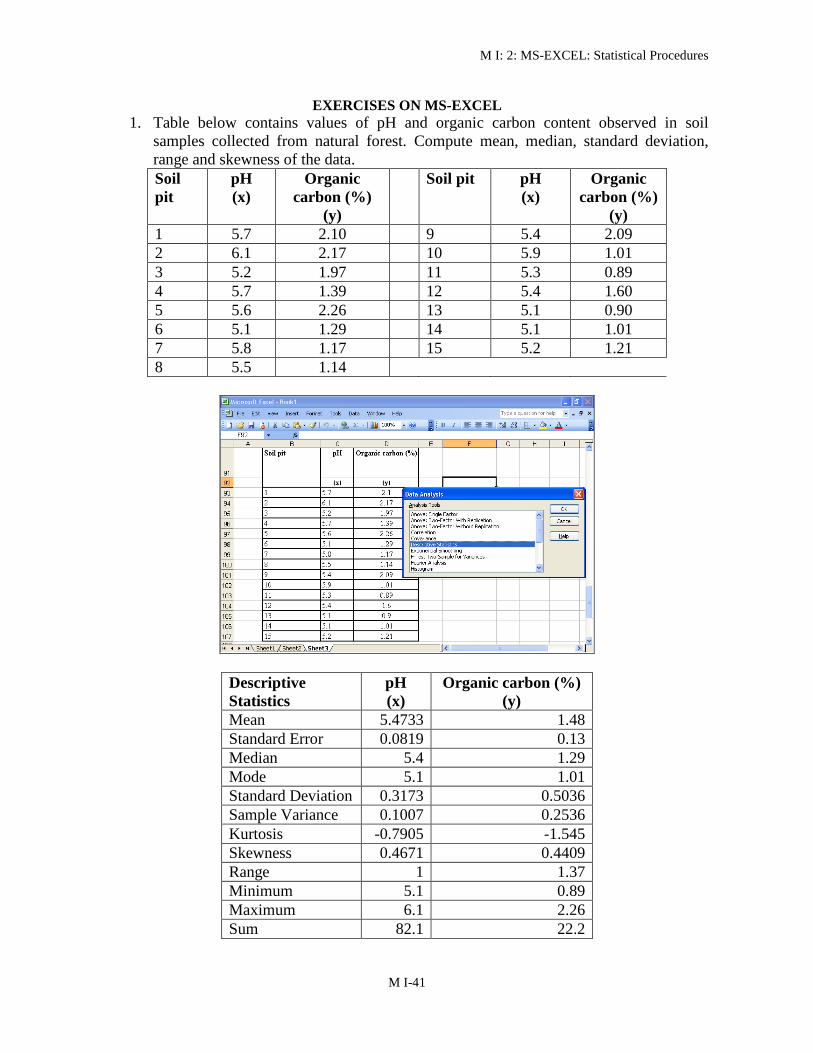
M I 2 MS-EXCEL Statistical Procedures
M I-41
EXERCISES ON MS-EXCEL
1 Table below contains values of pH and organic carbon content observed in soil
samples collected from natural forest Compute mean median standard deviation
range and skewness of the data
Soil
pit
pH
(x)
Organic
carbon ()
(y)
Soil pit pH
(x)
Organic
carbon ()
(y)
1 57 210 9 54 209
2 61 217 10 59 101
3 52 197 11 53 089
4 57 139 12 54 160
5 56 226 13 51 090
6 51 129 14 51 101
7 58 117 15 52 121
8 55 114
Descriptive
Statistics
pH
(x)
Organic carbon ()
(y)
Mean 54733 148
Standard Error 00819 013
Median 54 129
Mode 51 101
Standard Deviation 03173 05036
Sample Variance 01007 02536
Kurtosis -07905 -1545
Skewness 04671 04409
Range 1 137
Minimum 51 089
Maximum 61 226
Sum 821 222
M I 2 MS-EXCEL Statistical Procedures
M I-42
Count 15 15
2 Consider the following data on various characteristics of a crop
Pp Ph ngl yield
142 0525 82 247
143 064 95 476
107 066 93 331
78 066 75 197
100 046 59 134
865 0345 64 114
1035 086 64 15
15599 033 75 203
8088 0285 84 254
10977 059 106 49
6177 0265 83 291
7911 066 116 276
15599 042 81 059
6181 034 94 084
745 063 84 387
97 0705 72 447
9314 068 64 331
3743 0665 84 157
3644 0275 74 053
51 028 74 115
104 028 98 108
49 049 48 183
5466 0385 55 076
5555 0265 5 043
8844 098 5 408
9955 0645 96 283
6399 0635 56 257
10177 029 82 742
13866 072 99 262
9022 063 84 2
(i) Sort yield in ascending order and filter the data ph less than 03 or greater than 06
from the data
(ii) Find the correlation coefficient and fit the multiple regression equation by taking yield
as dependent variable
3 Let A B and C be three matrices as follows
A
31113519382765391642
B
1891427531
C
5582116632755328876348132
Find (i) AB (ii) C-1
(iii) A (iv) AT
M I 2 MS-EXCEL Statistical Procedures
M I-43
4 Draw line graph for the following data on a tree species
Year Height (cm) Diameter
1981 21 50
1982 34 80
1983 11 90
1984 13 30
1985 15 24
1986 55 55
1987 30 69
1988 50 91
1989 23 100
1990 22 25
1991 37 34
1992 38 62
1993 37 70
1994 11 81
1995 20 90
1996 16 37
1997 54 90
1998 33 40
1999 12 67
2000 19 77
M I 2 MS-EXCEL Statistical Procedures
M I-44
Also draw a bar diagram using the above data
5 The table below lists plant height in cm of seedlings of rice belonging to the two
varieties Examine whether the two samples are coming from populations having
equal variance using F-test Further test whether the average height of the two groups
are the same using appropriate t-test
Plot Group
I
Group II
1 230 85
2 174 96
3 170 77
4 205 101
5 227 97
6 240 132
7 225 103
8 227 91
9 194 105
10 188 74
F-Test Two-Sample for Variances
Variable 1 Variable 2
Mean 208 961
Variance 636 27143
Observations 10 10
Df 9 9
F 23431
P(Flt=f) one-
tail 01103
F Critical
one-tail 31789
Height and diameter of a tree species
over years
0
10
20
30
40
50
60
19
81
19
82
19
83
19
84
19
85
19
86
19
87
19
88
19
89
19
90
19
91
19
92
19
93
19
94
19
95
19
96
19
97
19
98
19
99
20
00
Year
Mea
sure
men
ts i
n c
ms
Height (cm)
Diameter
M I 2 MS-EXCEL Statistical Procedures
M I-45
t-Test Two-Sample Assuming Equal Variances
Variable 1 Variable 2
Mean 208 961
Variance 636 27143
Observations 10 10
Pooled Variance 45372
Hypothesized Mean
Difference 0
Df 18
t Stat 117469
P(Tlt=t) one-tail 35537E-10
t Critical one-tail 17341
P(Tlt=t) two-tail 71073E-10
t Critical two-tail 21009
6 Examine whether the average organic carbon content measured from two layers of a
set of soil pits from a pasture are same using paired t-test from the data given below
Organic carbon () OUTPUT
Soil
pit
Layer 1
(x)
Layer 2
(y)
x y
1 159 121 Mean 145 1269
2 139 092 Variance 0032 00613
3 164 131 Observations 10 10
4 117 152 Pearson Correlation -06249
5 127 162 Hypothesized Mean
Difference 0
6 158 091 df 9
7 164 123 t Stat 14845
8 153 121 P(Tlt=t) one-tail 00859
9 121 158 t Critical one-tail 18331
10 148 118 P(Tlt=t) two-tail 01718
t Critical two-tail 22622
7 Mycelial growth in terms of diameter of the colony (mm) of R solani isolates on PDA
medium after 14 hours of incubation is given in the table below Carry out the CRD
analysis for the data And draw your inferences
R solani isolates Mycelial growth
Repl 1 Repl 2 Repl 3
RS 1 290 280 290
RS 2 335 315 290
RS 3 265 300
RS 4 485 465 490
M I 2 MS-EXCEL Statistical Procedures
M I-46
RS 5 345 310
ANOVA
Source of
Variation SS df MS F P-value F crit
Treatments 7626859 4 1906715 573808 626E-06 38379
Error 2658333 8 3322917
Total 7892692 12
8 Following is the data on mean yield in kg per plot of an experiment conducted to
compare the performance of 8 treatments using a Randomized Complete Block design
with 3 replications Perform the analysis of variance
Treatment
(Provenance)
Replication
I II III
1 3085 3801 3510
2 3024 2843 3593
3 3094 3164 3495
4 2989 2912 3675
5 2152 2407 2076
6 2538 3214 3219
7 2289 1966 2692
8 2944 2495 3799
ANOVA
Source of
Variation SS df MS F P-value F crit
Treatments 4264549 7 609221 60497 00021 27642
Blocks 1109798 2 554899 55103 00172 37389
Error 1409842 14 100703
Total 6784189 23
9 From the following data make a summary table for finding out the average of X9 for
various years and various levels of X6 using pivot table and pivot chart report option
of MS-Excel
YR X1 X2 X3 X4 X5 X6 X7 X8 X9 X10 X11
1995 1 1 40 30 0 60 40 4861 5208 5556 5694
1995 1 2 40 30 0 60 40 4167 4444 4861 5035
1995 2 3 40 30 0 60 40 4618 4653 4653 5174
1995 2 4 40 30 0 60 40 4028 4167 4514 4722
1995 2 5 40 30 0 60 40 4306 4514 4653 4861
1996 2 1 40 30 0 60 40 6000 5750 5499 6250
1996 2 2 40 30 0 60 40 5646 5000 5250 5444
1996 2 3 40 30 0 60 40 4799 5097 4896 5299
1996 2 4 40 30 0 60 40 5250 5299 4194 4847
M I 2 MS-EXCEL Statistical Procedures
M I-47
1996 3 1 40 30 0 60 40 5139 5417 5764 5903
1996 3 2 40 30 0 60 40 5417 5694 6007 6111
1996 4 1 40 30 0 60 40 6300 7450 7750 8000
1996 4 2 40 30 0 60 40 6350 7850 7988 8200
1996 4 3 40 30 0 60 40 5750 6400 6600 6700
1996 4 4 40 30 0 60 40 6000 7250 7450 7681
1996 5 1 40 30 0 60 40 3396 4090 5056 5403
1996 5 2 40 30 0 60 40 5194 5000 6000 6500
1996 5 3 40 30 0 60 40 4299 4250 4750 5250
1996 6 1 40 30 0 60 40 4944 5194 5000 5097
1996 6 2 40 30 0 60 40 5395 5499 5499 5597
1996 6 3 40 30 0 60 40 3444 5646 5000 5000
1996 6 4 40 30 0 60 40 6250 6500 6646 6750
1997 1 1 120 30 30 120 60 5839 6248 6199 6335
1997 1 2 120 30 30 120 60 5590 5652 5702 5851
1997 2 1 120 30 30 120 60 4497 4794 4894 5205
1997 2 2 120 30 30 120 60 4696 5006 5304 5702
1997 2 3 120 30 30 120 60 4398 4596 4894 5304
1997 2 4 120 30 30 120 60 4497 5503 5702 6099
1997 3 1 120 30 30 120 60 4199 5602 5801 6000
1997 3 2 120 30 30 120 60 3404 3901 4199 4497
1997 3 3 120 30 30 120 60 3602 5404 5503 5801
1997 3 4 120 30 30 120 60 3602 4297 4497 4696
1997 4 1 120 30 30 120 60 3205 3801 4199 4894
1997 4 2 120 30 30 120 60 3801 4794 6099 6298
1997 4 3 120 30 30 120 60 3503 5205 6298 6795
1997 4 4 120 30 30 120 60 3205 4894 5503 6199
1997 5 1 120 30 30 120 60 4199 4099 4199 4297
1997 5 2 120 30 30 120 60 3304 3702 3602 3801
1997 5 3 120 30 30 120 60 2596 2894 3106 3205
1998 1 1 40 30 0 60 40 3727 3106 3404 3503
1998 1 2 40 30 0 60 40 4894 4348 4447 4534
1998 1 3 40 30 0 60 40 2696 2795 3056 3205
1998 2 2 40 30 0 60 40 5503 4298 4497 4795
1998 2 3 40 30 0 60 40 5006 3702 3702 3901
OUTPUT
Average of X9 X6
YR 60 120 Grand Total
1995 45972 45972
1996 57285882 57285882
1997 47289412 47289412
1998 36498 36498
Grand Total 51341111 47289412 49775682
M I 2 MS-EXCEL Statistical Procedures
M I-48
10 From the data given in problem 10 sort X10 in ascending order Also filter the data for
X11 lt 4200 or X11 gt 5000
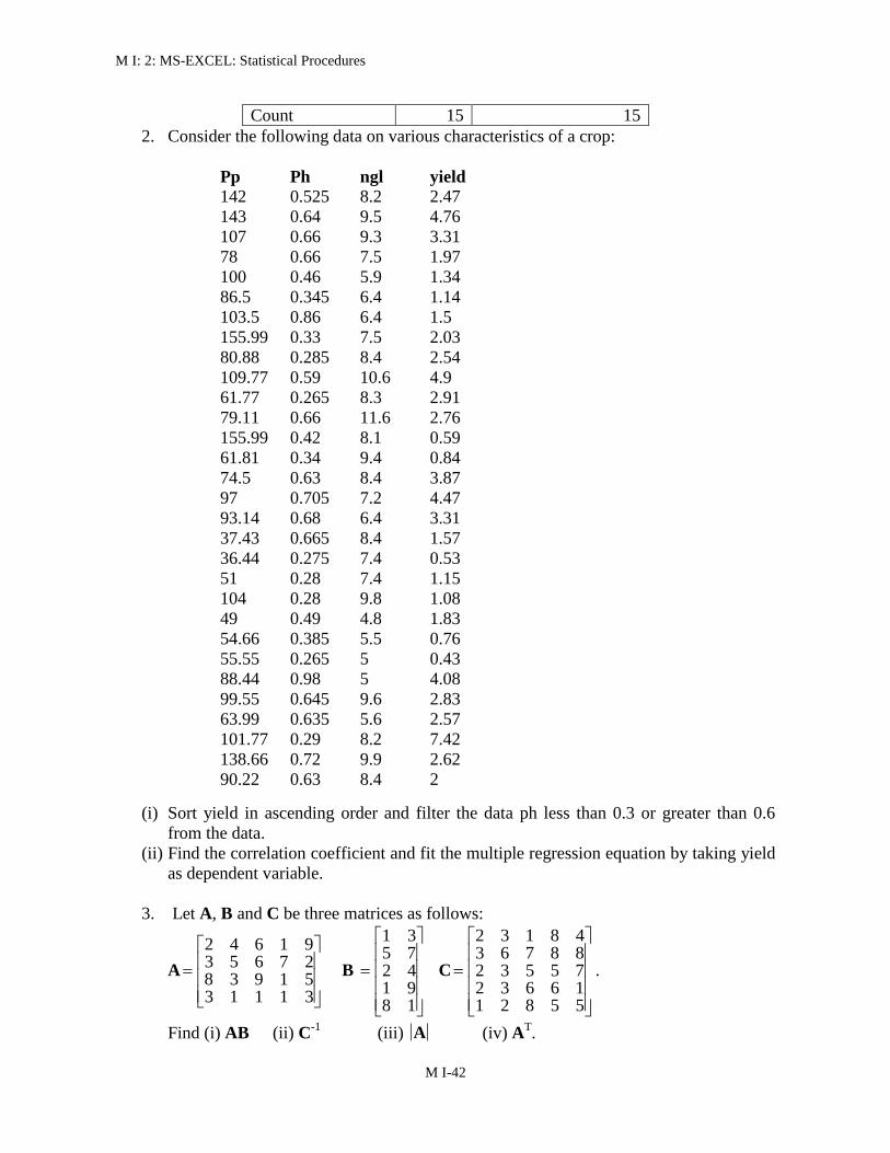
M I 2 MS-EXCEL Statistical Procedures
M I-42
Count 15 15
2 Consider the following data on various characteristics of a crop
Pp Ph ngl yield
142 0525 82 247
143 064 95 476
107 066 93 331
78 066 75 197
100 046 59 134
865 0345 64 114
1035 086 64 15
15599 033 75 203
8088 0285 84 254
10977 059 106 49
6177 0265 83 291
7911 066 116 276
15599 042 81 059
6181 034 94 084
745 063 84 387
97 0705 72 447
9314 068 64 331
3743 0665 84 157
3644 0275 74 053
51 028 74 115
104 028 98 108
49 049 48 183
5466 0385 55 076
5555 0265 5 043
8844 098 5 408
9955 0645 96 283
6399 0635 56 257
10177 029 82 742
13866 072 99 262
9022 063 84 2
(i) Sort yield in ascending order and filter the data ph less than 03 or greater than 06
from the data
(ii) Find the correlation coefficient and fit the multiple regression equation by taking yield
as dependent variable
3 Let A B and C be three matrices as follows
A
31113519382765391642
B
1891427531
C
5582116632755328876348132
Find (i) AB (ii) C-1
(iii) A (iv) AT
M I 2 MS-EXCEL Statistical Procedures
M I-43
4 Draw line graph for the following data on a tree species
Year Height (cm) Diameter
1981 21 50
1982 34 80
1983 11 90
1984 13 30
1985 15 24
1986 55 55
1987 30 69
1988 50 91
1989 23 100
1990 22 25
1991 37 34
1992 38 62
1993 37 70
1994 11 81
1995 20 90
1996 16 37
1997 54 90
1998 33 40
1999 12 67
2000 19 77
M I 2 MS-EXCEL Statistical Procedures
M I-44
Also draw a bar diagram using the above data
5 The table below lists plant height in cm of seedlings of rice belonging to the two
varieties Examine whether the two samples are coming from populations having
equal variance using F-test Further test whether the average height of the two groups
are the same using appropriate t-test
Plot Group
I
Group II
1 230 85
2 174 96
3 170 77
4 205 101
5 227 97
6 240 132
7 225 103
8 227 91
9 194 105
10 188 74
F-Test Two-Sample for Variances
Variable 1 Variable 2
Mean 208 961
Variance 636 27143
Observations 10 10
Df 9 9
F 23431
P(Flt=f) one-
tail 01103
F Critical
one-tail 31789
Height and diameter of a tree species
over years
0
10
20
30
40
50
60
19
81
19
82
19
83
19
84
19
85
19
86
19
87
19
88
19
89
19
90
19
91
19
92
19
93
19
94
19
95
19
96
19
97
19
98
19
99
20
00
Year
Mea
sure
men
ts i
n c
ms
Height (cm)
Diameter
M I 2 MS-EXCEL Statistical Procedures
M I-45
t-Test Two-Sample Assuming Equal Variances
Variable 1 Variable 2
Mean 208 961
Variance 636 27143
Observations 10 10
Pooled Variance 45372
Hypothesized Mean
Difference 0
Df 18
t Stat 117469
P(Tlt=t) one-tail 35537E-10
t Critical one-tail 17341
P(Tlt=t) two-tail 71073E-10
t Critical two-tail 21009
6 Examine whether the average organic carbon content measured from two layers of a
set of soil pits from a pasture are same using paired t-test from the data given below
Organic carbon () OUTPUT
Soil
pit
Layer 1
(x)
Layer 2
(y)
x y
1 159 121 Mean 145 1269
2 139 092 Variance 0032 00613
3 164 131 Observations 10 10
4 117 152 Pearson Correlation -06249
5 127 162 Hypothesized Mean
Difference 0
6 158 091 df 9
7 164 123 t Stat 14845
8 153 121 P(Tlt=t) one-tail 00859
9 121 158 t Critical one-tail 18331
10 148 118 P(Tlt=t) two-tail 01718
t Critical two-tail 22622
7 Mycelial growth in terms of diameter of the colony (mm) of R solani isolates on PDA
medium after 14 hours of incubation is given in the table below Carry out the CRD
analysis for the data And draw your inferences
R solani isolates Mycelial growth
Repl 1 Repl 2 Repl 3
RS 1 290 280 290
RS 2 335 315 290
RS 3 265 300
RS 4 485 465 490
M I 2 MS-EXCEL Statistical Procedures
M I-46
RS 5 345 310
ANOVA
Source of
Variation SS df MS F P-value F crit
Treatments 7626859 4 1906715 573808 626E-06 38379
Error 2658333 8 3322917
Total 7892692 12
8 Following is the data on mean yield in kg per plot of an experiment conducted to
compare the performance of 8 treatments using a Randomized Complete Block design
with 3 replications Perform the analysis of variance
Treatment
(Provenance)
Replication
I II III
1 3085 3801 3510
2 3024 2843 3593
3 3094 3164 3495
4 2989 2912 3675
5 2152 2407 2076
6 2538 3214 3219
7 2289 1966 2692
8 2944 2495 3799
ANOVA
Source of
Variation SS df MS F P-value F crit
Treatments 4264549 7 609221 60497 00021 27642
Blocks 1109798 2 554899 55103 00172 37389
Error 1409842 14 100703
Total 6784189 23
9 From the following data make a summary table for finding out the average of X9 for
various years and various levels of X6 using pivot table and pivot chart report option
of MS-Excel
YR X1 X2 X3 X4 X5 X6 X7 X8 X9 X10 X11
1995 1 1 40 30 0 60 40 4861 5208 5556 5694
1995 1 2 40 30 0 60 40 4167 4444 4861 5035
1995 2 3 40 30 0 60 40 4618 4653 4653 5174
1995 2 4 40 30 0 60 40 4028 4167 4514 4722
1995 2 5 40 30 0 60 40 4306 4514 4653 4861
1996 2 1 40 30 0 60 40 6000 5750 5499 6250
1996 2 2 40 30 0 60 40 5646 5000 5250 5444
1996 2 3 40 30 0 60 40 4799 5097 4896 5299
1996 2 4 40 30 0 60 40 5250 5299 4194 4847
M I 2 MS-EXCEL Statistical Procedures
M I-47
1996 3 1 40 30 0 60 40 5139 5417 5764 5903
1996 3 2 40 30 0 60 40 5417 5694 6007 6111
1996 4 1 40 30 0 60 40 6300 7450 7750 8000
1996 4 2 40 30 0 60 40 6350 7850 7988 8200
1996 4 3 40 30 0 60 40 5750 6400 6600 6700
1996 4 4 40 30 0 60 40 6000 7250 7450 7681
1996 5 1 40 30 0 60 40 3396 4090 5056 5403
1996 5 2 40 30 0 60 40 5194 5000 6000 6500
1996 5 3 40 30 0 60 40 4299 4250 4750 5250
1996 6 1 40 30 0 60 40 4944 5194 5000 5097
1996 6 2 40 30 0 60 40 5395 5499 5499 5597
1996 6 3 40 30 0 60 40 3444 5646 5000 5000
1996 6 4 40 30 0 60 40 6250 6500 6646 6750
1997 1 1 120 30 30 120 60 5839 6248 6199 6335
1997 1 2 120 30 30 120 60 5590 5652 5702 5851
1997 2 1 120 30 30 120 60 4497 4794 4894 5205
1997 2 2 120 30 30 120 60 4696 5006 5304 5702
1997 2 3 120 30 30 120 60 4398 4596 4894 5304
1997 2 4 120 30 30 120 60 4497 5503 5702 6099
1997 3 1 120 30 30 120 60 4199 5602 5801 6000
1997 3 2 120 30 30 120 60 3404 3901 4199 4497
1997 3 3 120 30 30 120 60 3602 5404 5503 5801
1997 3 4 120 30 30 120 60 3602 4297 4497 4696
1997 4 1 120 30 30 120 60 3205 3801 4199 4894
1997 4 2 120 30 30 120 60 3801 4794 6099 6298
1997 4 3 120 30 30 120 60 3503 5205 6298 6795
1997 4 4 120 30 30 120 60 3205 4894 5503 6199
1997 5 1 120 30 30 120 60 4199 4099 4199 4297
1997 5 2 120 30 30 120 60 3304 3702 3602 3801
1997 5 3 120 30 30 120 60 2596 2894 3106 3205
1998 1 1 40 30 0 60 40 3727 3106 3404 3503
1998 1 2 40 30 0 60 40 4894 4348 4447 4534
1998 1 3 40 30 0 60 40 2696 2795 3056 3205
1998 2 2 40 30 0 60 40 5503 4298 4497 4795
1998 2 3 40 30 0 60 40 5006 3702 3702 3901
OUTPUT
Average of X9 X6
YR 60 120 Grand Total
1995 45972 45972
1996 57285882 57285882
1997 47289412 47289412
1998 36498 36498
Grand Total 51341111 47289412 49775682
M I 2 MS-EXCEL Statistical Procedures
M I-48
10 From the data given in problem 10 sort X10 in ascending order Also filter the data for
X11 lt 4200 or X11 gt 5000
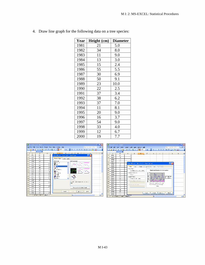
M I 2 MS-EXCEL Statistical Procedures
M I-43
4 Draw line graph for the following data on a tree species
Year Height (cm) Diameter
1981 21 50
1982 34 80
1983 11 90
1984 13 30
1985 15 24
1986 55 55
1987 30 69
1988 50 91
1989 23 100
1990 22 25
1991 37 34
1992 38 62
1993 37 70
1994 11 81
1995 20 90
1996 16 37
1997 54 90
1998 33 40
1999 12 67
2000 19 77
M I 2 MS-EXCEL Statistical Procedures
M I-44
Also draw a bar diagram using the above data
5 The table below lists plant height in cm of seedlings of rice belonging to the two
varieties Examine whether the two samples are coming from populations having
equal variance using F-test Further test whether the average height of the two groups
are the same using appropriate t-test
Plot Group
I
Group II
1 230 85
2 174 96
3 170 77
4 205 101
5 227 97
6 240 132
7 225 103
8 227 91
9 194 105
10 188 74
F-Test Two-Sample for Variances
Variable 1 Variable 2
Mean 208 961
Variance 636 27143
Observations 10 10
Df 9 9
F 23431
P(Flt=f) one-
tail 01103
F Critical
one-tail 31789
Height and diameter of a tree species
over years
0
10
20
30
40
50
60
19
81
19
82
19
83
19
84
19
85
19
86
19
87
19
88
19
89
19
90
19
91
19
92
19
93
19
94
19
95
19
96
19
97
19
98
19
99
20
00
Year
Mea
sure
men
ts i
n c
ms
Height (cm)
Diameter
M I 2 MS-EXCEL Statistical Procedures
M I-45
t-Test Two-Sample Assuming Equal Variances
Variable 1 Variable 2
Mean 208 961
Variance 636 27143
Observations 10 10
Pooled Variance 45372
Hypothesized Mean
Difference 0
Df 18
t Stat 117469
P(Tlt=t) one-tail 35537E-10
t Critical one-tail 17341
P(Tlt=t) two-tail 71073E-10
t Critical two-tail 21009
6 Examine whether the average organic carbon content measured from two layers of a
set of soil pits from a pasture are same using paired t-test from the data given below
Organic carbon () OUTPUT
Soil
pit
Layer 1
(x)
Layer 2
(y)
x y
1 159 121 Mean 145 1269
2 139 092 Variance 0032 00613
3 164 131 Observations 10 10
4 117 152 Pearson Correlation -06249
5 127 162 Hypothesized Mean
Difference 0
6 158 091 df 9
7 164 123 t Stat 14845
8 153 121 P(Tlt=t) one-tail 00859
9 121 158 t Critical one-tail 18331
10 148 118 P(Tlt=t) two-tail 01718
t Critical two-tail 22622
7 Mycelial growth in terms of diameter of the colony (mm) of R solani isolates on PDA
medium after 14 hours of incubation is given in the table below Carry out the CRD
analysis for the data And draw your inferences
R solani isolates Mycelial growth
Repl 1 Repl 2 Repl 3
RS 1 290 280 290
RS 2 335 315 290
RS 3 265 300
RS 4 485 465 490
M I 2 MS-EXCEL Statistical Procedures
M I-46
RS 5 345 310
ANOVA
Source of
Variation SS df MS F P-value F crit
Treatments 7626859 4 1906715 573808 626E-06 38379
Error 2658333 8 3322917
Total 7892692 12
8 Following is the data on mean yield in kg per plot of an experiment conducted to
compare the performance of 8 treatments using a Randomized Complete Block design
with 3 replications Perform the analysis of variance
Treatment
(Provenance)
Replication
I II III
1 3085 3801 3510
2 3024 2843 3593
3 3094 3164 3495
4 2989 2912 3675
5 2152 2407 2076
6 2538 3214 3219
7 2289 1966 2692
8 2944 2495 3799
ANOVA
Source of
Variation SS df MS F P-value F crit
Treatments 4264549 7 609221 60497 00021 27642
Blocks 1109798 2 554899 55103 00172 37389
Error 1409842 14 100703
Total 6784189 23
9 From the following data make a summary table for finding out the average of X9 for
various years and various levels of X6 using pivot table and pivot chart report option
of MS-Excel
YR X1 X2 X3 X4 X5 X6 X7 X8 X9 X10 X11
1995 1 1 40 30 0 60 40 4861 5208 5556 5694
1995 1 2 40 30 0 60 40 4167 4444 4861 5035
1995 2 3 40 30 0 60 40 4618 4653 4653 5174
1995 2 4 40 30 0 60 40 4028 4167 4514 4722
1995 2 5 40 30 0 60 40 4306 4514 4653 4861
1996 2 1 40 30 0 60 40 6000 5750 5499 6250
1996 2 2 40 30 0 60 40 5646 5000 5250 5444
1996 2 3 40 30 0 60 40 4799 5097 4896 5299
1996 2 4 40 30 0 60 40 5250 5299 4194 4847
M I 2 MS-EXCEL Statistical Procedures
M I-47
1996 3 1 40 30 0 60 40 5139 5417 5764 5903
1996 3 2 40 30 0 60 40 5417 5694 6007 6111
1996 4 1 40 30 0 60 40 6300 7450 7750 8000
1996 4 2 40 30 0 60 40 6350 7850 7988 8200
1996 4 3 40 30 0 60 40 5750 6400 6600 6700
1996 4 4 40 30 0 60 40 6000 7250 7450 7681
1996 5 1 40 30 0 60 40 3396 4090 5056 5403
1996 5 2 40 30 0 60 40 5194 5000 6000 6500
1996 5 3 40 30 0 60 40 4299 4250 4750 5250
1996 6 1 40 30 0 60 40 4944 5194 5000 5097
1996 6 2 40 30 0 60 40 5395 5499 5499 5597
1996 6 3 40 30 0 60 40 3444 5646 5000 5000
1996 6 4 40 30 0 60 40 6250 6500 6646 6750
1997 1 1 120 30 30 120 60 5839 6248 6199 6335
1997 1 2 120 30 30 120 60 5590 5652 5702 5851
1997 2 1 120 30 30 120 60 4497 4794 4894 5205
1997 2 2 120 30 30 120 60 4696 5006 5304 5702
1997 2 3 120 30 30 120 60 4398 4596 4894 5304
1997 2 4 120 30 30 120 60 4497 5503 5702 6099
1997 3 1 120 30 30 120 60 4199 5602 5801 6000
1997 3 2 120 30 30 120 60 3404 3901 4199 4497
1997 3 3 120 30 30 120 60 3602 5404 5503 5801
1997 3 4 120 30 30 120 60 3602 4297 4497 4696
1997 4 1 120 30 30 120 60 3205 3801 4199 4894
1997 4 2 120 30 30 120 60 3801 4794 6099 6298
1997 4 3 120 30 30 120 60 3503 5205 6298 6795
1997 4 4 120 30 30 120 60 3205 4894 5503 6199
1997 5 1 120 30 30 120 60 4199 4099 4199 4297
1997 5 2 120 30 30 120 60 3304 3702 3602 3801
1997 5 3 120 30 30 120 60 2596 2894 3106 3205
1998 1 1 40 30 0 60 40 3727 3106 3404 3503
1998 1 2 40 30 0 60 40 4894 4348 4447 4534
1998 1 3 40 30 0 60 40 2696 2795 3056 3205
1998 2 2 40 30 0 60 40 5503 4298 4497 4795
1998 2 3 40 30 0 60 40 5006 3702 3702 3901
OUTPUT
Average of X9 X6
YR 60 120 Grand Total
1995 45972 45972
1996 57285882 57285882
1997 47289412 47289412
1998 36498 36498
Grand Total 51341111 47289412 49775682
M I 2 MS-EXCEL Statistical Procedures
M I-48
10 From the data given in problem 10 sort X10 in ascending order Also filter the data for
X11 lt 4200 or X11 gt 5000
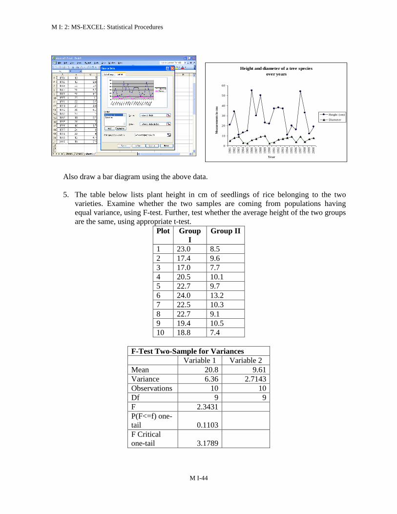
M I 2 MS-EXCEL Statistical Procedures
M I-44
Also draw a bar diagram using the above data
5 The table below lists plant height in cm of seedlings of rice belonging to the two
varieties Examine whether the two samples are coming from populations having
equal variance using F-test Further test whether the average height of the two groups
are the same using appropriate t-test
Plot Group
I
Group II
1 230 85
2 174 96
3 170 77
4 205 101
5 227 97
6 240 132
7 225 103
8 227 91
9 194 105
10 188 74
F-Test Two-Sample for Variances
Variable 1 Variable 2
Mean 208 961
Variance 636 27143
Observations 10 10
Df 9 9
F 23431
P(Flt=f) one-
tail 01103
F Critical
one-tail 31789
Height and diameter of a tree species
over years
0
10
20
30
40
50
60
19
81
19
82
19
83
19
84
19
85
19
86
19
87
19
88
19
89
19
90
19
91
19
92
19
93
19
94
19
95
19
96
19
97
19
98
19
99
20
00
Year
Mea
sure
men
ts i
n c
ms
Height (cm)
Diameter
M I 2 MS-EXCEL Statistical Procedures
M I-45
t-Test Two-Sample Assuming Equal Variances
Variable 1 Variable 2
Mean 208 961
Variance 636 27143
Observations 10 10
Pooled Variance 45372
Hypothesized Mean
Difference 0
Df 18
t Stat 117469
P(Tlt=t) one-tail 35537E-10
t Critical one-tail 17341
P(Tlt=t) two-tail 71073E-10
t Critical two-tail 21009
6 Examine whether the average organic carbon content measured from two layers of a
set of soil pits from a pasture are same using paired t-test from the data given below
Organic carbon () OUTPUT
Soil
pit
Layer 1
(x)
Layer 2
(y)
x y
1 159 121 Mean 145 1269
2 139 092 Variance 0032 00613
3 164 131 Observations 10 10
4 117 152 Pearson Correlation -06249
5 127 162 Hypothesized Mean
Difference 0
6 158 091 df 9
7 164 123 t Stat 14845
8 153 121 P(Tlt=t) one-tail 00859
9 121 158 t Critical one-tail 18331
10 148 118 P(Tlt=t) two-tail 01718
t Critical two-tail 22622
7 Mycelial growth in terms of diameter of the colony (mm) of R solani isolates on PDA
medium after 14 hours of incubation is given in the table below Carry out the CRD
analysis for the data And draw your inferences
R solani isolates Mycelial growth
Repl 1 Repl 2 Repl 3
RS 1 290 280 290
RS 2 335 315 290
RS 3 265 300
RS 4 485 465 490
M I 2 MS-EXCEL Statistical Procedures
M I-46
RS 5 345 310
ANOVA
Source of
Variation SS df MS F P-value F crit
Treatments 7626859 4 1906715 573808 626E-06 38379
Error 2658333 8 3322917
Total 7892692 12
8 Following is the data on mean yield in kg per plot of an experiment conducted to
compare the performance of 8 treatments using a Randomized Complete Block design
with 3 replications Perform the analysis of variance
Treatment
(Provenance)
Replication
I II III
1 3085 3801 3510
2 3024 2843 3593
3 3094 3164 3495
4 2989 2912 3675
5 2152 2407 2076
6 2538 3214 3219
7 2289 1966 2692
8 2944 2495 3799
ANOVA
Source of
Variation SS df MS F P-value F crit
Treatments 4264549 7 609221 60497 00021 27642
Blocks 1109798 2 554899 55103 00172 37389
Error 1409842 14 100703
Total 6784189 23
9 From the following data make a summary table for finding out the average of X9 for
various years and various levels of X6 using pivot table and pivot chart report option
of MS-Excel
YR X1 X2 X3 X4 X5 X6 X7 X8 X9 X10 X11
1995 1 1 40 30 0 60 40 4861 5208 5556 5694
1995 1 2 40 30 0 60 40 4167 4444 4861 5035
1995 2 3 40 30 0 60 40 4618 4653 4653 5174
1995 2 4 40 30 0 60 40 4028 4167 4514 4722
1995 2 5 40 30 0 60 40 4306 4514 4653 4861
1996 2 1 40 30 0 60 40 6000 5750 5499 6250
1996 2 2 40 30 0 60 40 5646 5000 5250 5444
1996 2 3 40 30 0 60 40 4799 5097 4896 5299
1996 2 4 40 30 0 60 40 5250 5299 4194 4847
M I 2 MS-EXCEL Statistical Procedures
M I-47
1996 3 1 40 30 0 60 40 5139 5417 5764 5903
1996 3 2 40 30 0 60 40 5417 5694 6007 6111
1996 4 1 40 30 0 60 40 6300 7450 7750 8000
1996 4 2 40 30 0 60 40 6350 7850 7988 8200
1996 4 3 40 30 0 60 40 5750 6400 6600 6700
1996 4 4 40 30 0 60 40 6000 7250 7450 7681
1996 5 1 40 30 0 60 40 3396 4090 5056 5403
1996 5 2 40 30 0 60 40 5194 5000 6000 6500
1996 5 3 40 30 0 60 40 4299 4250 4750 5250
1996 6 1 40 30 0 60 40 4944 5194 5000 5097
1996 6 2 40 30 0 60 40 5395 5499 5499 5597
1996 6 3 40 30 0 60 40 3444 5646 5000 5000
1996 6 4 40 30 0 60 40 6250 6500 6646 6750
1997 1 1 120 30 30 120 60 5839 6248 6199 6335
1997 1 2 120 30 30 120 60 5590 5652 5702 5851
1997 2 1 120 30 30 120 60 4497 4794 4894 5205
1997 2 2 120 30 30 120 60 4696 5006 5304 5702
1997 2 3 120 30 30 120 60 4398 4596 4894 5304
1997 2 4 120 30 30 120 60 4497 5503 5702 6099
1997 3 1 120 30 30 120 60 4199 5602 5801 6000
1997 3 2 120 30 30 120 60 3404 3901 4199 4497
1997 3 3 120 30 30 120 60 3602 5404 5503 5801
1997 3 4 120 30 30 120 60 3602 4297 4497 4696
1997 4 1 120 30 30 120 60 3205 3801 4199 4894
1997 4 2 120 30 30 120 60 3801 4794 6099 6298
1997 4 3 120 30 30 120 60 3503 5205 6298 6795
1997 4 4 120 30 30 120 60 3205 4894 5503 6199
1997 5 1 120 30 30 120 60 4199 4099 4199 4297
1997 5 2 120 30 30 120 60 3304 3702 3602 3801
1997 5 3 120 30 30 120 60 2596 2894 3106 3205
1998 1 1 40 30 0 60 40 3727 3106 3404 3503
1998 1 2 40 30 0 60 40 4894 4348 4447 4534
1998 1 3 40 30 0 60 40 2696 2795 3056 3205
1998 2 2 40 30 0 60 40 5503 4298 4497 4795
1998 2 3 40 30 0 60 40 5006 3702 3702 3901
OUTPUT
Average of X9 X6
YR 60 120 Grand Total
1995 45972 45972
1996 57285882 57285882
1997 47289412 47289412
1998 36498 36498
Grand Total 51341111 47289412 49775682
M I 2 MS-EXCEL Statistical Procedures
M I-48
10 From the data given in problem 10 sort X10 in ascending order Also filter the data for
X11 lt 4200 or X11 gt 5000
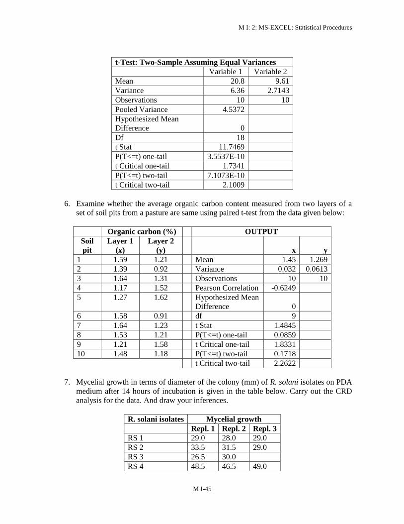
M I 2 MS-EXCEL Statistical Procedures
M I-45
t-Test Two-Sample Assuming Equal Variances
Variable 1 Variable 2
Mean 208 961
Variance 636 27143
Observations 10 10
Pooled Variance 45372
Hypothesized Mean
Difference 0
Df 18
t Stat 117469
P(Tlt=t) one-tail 35537E-10
t Critical one-tail 17341
P(Tlt=t) two-tail 71073E-10
t Critical two-tail 21009
6 Examine whether the average organic carbon content measured from two layers of a
set of soil pits from a pasture are same using paired t-test from the data given below
Organic carbon () OUTPUT
Soil
pit
Layer 1
(x)
Layer 2
(y)
x y
1 159 121 Mean 145 1269
2 139 092 Variance 0032 00613
3 164 131 Observations 10 10
4 117 152 Pearson Correlation -06249
5 127 162 Hypothesized Mean
Difference 0
6 158 091 df 9
7 164 123 t Stat 14845
8 153 121 P(Tlt=t) one-tail 00859
9 121 158 t Critical one-tail 18331
10 148 118 P(Tlt=t) two-tail 01718
t Critical two-tail 22622
7 Mycelial growth in terms of diameter of the colony (mm) of R solani isolates on PDA
medium after 14 hours of incubation is given in the table below Carry out the CRD
analysis for the data And draw your inferences
R solani isolates Mycelial growth
Repl 1 Repl 2 Repl 3
RS 1 290 280 290
RS 2 335 315 290
RS 3 265 300
RS 4 485 465 490
M I 2 MS-EXCEL Statistical Procedures
M I-46
RS 5 345 310
ANOVA
Source of
Variation SS df MS F P-value F crit
Treatments 7626859 4 1906715 573808 626E-06 38379
Error 2658333 8 3322917
Total 7892692 12
8 Following is the data on mean yield in kg per plot of an experiment conducted to
compare the performance of 8 treatments using a Randomized Complete Block design
with 3 replications Perform the analysis of variance
Treatment
(Provenance)
Replication
I II III
1 3085 3801 3510
2 3024 2843 3593
3 3094 3164 3495
4 2989 2912 3675
5 2152 2407 2076
6 2538 3214 3219
7 2289 1966 2692
8 2944 2495 3799
ANOVA
Source of
Variation SS df MS F P-value F crit
Treatments 4264549 7 609221 60497 00021 27642
Blocks 1109798 2 554899 55103 00172 37389
Error 1409842 14 100703
Total 6784189 23
9 From the following data make a summary table for finding out the average of X9 for
various years and various levels of X6 using pivot table and pivot chart report option
of MS-Excel
YR X1 X2 X3 X4 X5 X6 X7 X8 X9 X10 X11
1995 1 1 40 30 0 60 40 4861 5208 5556 5694
1995 1 2 40 30 0 60 40 4167 4444 4861 5035
1995 2 3 40 30 0 60 40 4618 4653 4653 5174
1995 2 4 40 30 0 60 40 4028 4167 4514 4722
1995 2 5 40 30 0 60 40 4306 4514 4653 4861
1996 2 1 40 30 0 60 40 6000 5750 5499 6250
1996 2 2 40 30 0 60 40 5646 5000 5250 5444
1996 2 3 40 30 0 60 40 4799 5097 4896 5299
1996 2 4 40 30 0 60 40 5250 5299 4194 4847
M I 2 MS-EXCEL Statistical Procedures
M I-47
1996 3 1 40 30 0 60 40 5139 5417 5764 5903
1996 3 2 40 30 0 60 40 5417 5694 6007 6111
1996 4 1 40 30 0 60 40 6300 7450 7750 8000
1996 4 2 40 30 0 60 40 6350 7850 7988 8200
1996 4 3 40 30 0 60 40 5750 6400 6600 6700
1996 4 4 40 30 0 60 40 6000 7250 7450 7681
1996 5 1 40 30 0 60 40 3396 4090 5056 5403
1996 5 2 40 30 0 60 40 5194 5000 6000 6500
1996 5 3 40 30 0 60 40 4299 4250 4750 5250
1996 6 1 40 30 0 60 40 4944 5194 5000 5097
1996 6 2 40 30 0 60 40 5395 5499 5499 5597
1996 6 3 40 30 0 60 40 3444 5646 5000 5000
1996 6 4 40 30 0 60 40 6250 6500 6646 6750
1997 1 1 120 30 30 120 60 5839 6248 6199 6335
1997 1 2 120 30 30 120 60 5590 5652 5702 5851
1997 2 1 120 30 30 120 60 4497 4794 4894 5205
1997 2 2 120 30 30 120 60 4696 5006 5304 5702
1997 2 3 120 30 30 120 60 4398 4596 4894 5304
1997 2 4 120 30 30 120 60 4497 5503 5702 6099
1997 3 1 120 30 30 120 60 4199 5602 5801 6000
1997 3 2 120 30 30 120 60 3404 3901 4199 4497
1997 3 3 120 30 30 120 60 3602 5404 5503 5801
1997 3 4 120 30 30 120 60 3602 4297 4497 4696
1997 4 1 120 30 30 120 60 3205 3801 4199 4894
1997 4 2 120 30 30 120 60 3801 4794 6099 6298
1997 4 3 120 30 30 120 60 3503 5205 6298 6795
1997 4 4 120 30 30 120 60 3205 4894 5503 6199
1997 5 1 120 30 30 120 60 4199 4099 4199 4297
1997 5 2 120 30 30 120 60 3304 3702 3602 3801
1997 5 3 120 30 30 120 60 2596 2894 3106 3205
1998 1 1 40 30 0 60 40 3727 3106 3404 3503
1998 1 2 40 30 0 60 40 4894 4348 4447 4534
1998 1 3 40 30 0 60 40 2696 2795 3056 3205
1998 2 2 40 30 0 60 40 5503 4298 4497 4795
1998 2 3 40 30 0 60 40 5006 3702 3702 3901
OUTPUT
Average of X9 X6
YR 60 120 Grand Total
1995 45972 45972
1996 57285882 57285882
1997 47289412 47289412
1998 36498 36498
Grand Total 51341111 47289412 49775682
M I 2 MS-EXCEL Statistical Procedures
M I-48
10 From the data given in problem 10 sort X10 in ascending order Also filter the data for
X11 lt 4200 or X11 gt 5000
M I 2 MS-EXCEL Statistical Procedures
M I-47
1996 3 1 40 30 0 60 40 5139 5417 5764 5903
1996 3 2 40 30 0 60 40 5417 5694 6007 6111
1996 4 1 40 30 0 60 40 6300 7450 7750 8000
1996 4 2 40 30 0 60 40 6350 7850 7988 8200
1996 4 3 40 30 0 60 40 5750 6400 6600 6700
1996 4 4 40 30 0 60 40 6000 7250 7450 7681
1996 5 1 40 30 0 60 40 3396 4090 5056 5403
1996 5 2 40 30 0 60 40 5194 5000 6000 6500
1996 5 3 40 30 0 60 40 4299 4250 4750 5250
1996 6 1 40 30 0 60 40 4944 5194 5000 5097
1996 6 2 40 30 0 60 40 5395 5499 5499 5597
1996 6 3 40 30 0 60 40 3444 5646 5000 5000
1996 6 4 40 30 0 60 40 6250 6500 6646 6750
1997 1 1 120 30 30 120 60 5839 6248 6199 6335
1997 1 2 120 30 30 120 60 5590 5652 5702 5851
1997 2 1 120 30 30 120 60 4497 4794 4894 5205
1997 2 2 120 30 30 120 60 4696 5006 5304 5702
1997 2 3 120 30 30 120 60 4398 4596 4894 5304
1997 2 4 120 30 30 120 60 4497 5503 5702 6099
1997 3 1 120 30 30 120 60 4199 5602 5801 6000
1997 3 2 120 30 30 120 60 3404 3901 4199 4497
1997 3 3 120 30 30 120 60 3602 5404 5503 5801
1997 3 4 120 30 30 120 60 3602 4297 4497 4696
1997 4 1 120 30 30 120 60 3205 3801 4199 4894
1997 4 2 120 30 30 120 60 3801 4794 6099 6298
1997 4 3 120 30 30 120 60 3503 5205 6298 6795
1997 4 4 120 30 30 120 60 3205 4894 5503 6199
1997 5 1 120 30 30 120 60 4199 4099 4199 4297
1997 5 2 120 30 30 120 60 3304 3702 3602 3801
1997 5 3 120 30 30 120 60 2596 2894 3106 3205
1998 1 1 40 30 0 60 40 3727 3106 3404 3503
1998 1 2 40 30 0 60 40 4894 4348 4447 4534
1998 1 3 40 30 0 60 40 2696 2795 3056 3205
1998 2 2 40 30 0 60 40 5503 4298 4497 4795
1998 2 3 40 30 0 60 40 5006 3702 3702 3901
OUTPUT
Average of X9 X6
YR 60 120 Grand Total
1995 45972 45972
1996 57285882 57285882
1997 47289412 47289412
1998 36498 36498
Grand Total 51341111 47289412 49775682
M I 2 MS-EXCEL Statistical Procedures
M I-48
10 From the data given in problem 10 sort X10 in ascending order Also filter the data for
X11 lt 4200 or X11 gt 5000

M I 2 MS-EXCEL Statistical Procedures
M I-48
10 From the data given in problem 10 sort X10 in ascending order Also filter the data for
X11 lt 4200 or X11 gt 5000