MRI denoising via phase error estimation

Dylan Tisdall and M. Stella Atkins

Simon Fraser University, 8888 University Drive, Burnaby, BC, Canada

ABSTRACT

If the phase error at each pixel in a complex-valued MRI image is known the noise in the image can be reducedresulting in improved detection of medically significant details. However, given a complex-valued MRI image,estimating the phase error at each pixel is a difficult problem. Several approaches have previously been suggestedincluding non-linear least squares fitting and smoothing filters. We propose a new scheme based on iterativelyapplying a series of non-linear filters, each used to modify the estimate into greater agreement with one pieceof knowledge about the problem, until the output converges to a stable estimate. We compare our results withother phase estimation and MRI denoising schemes using synthetic data.

Keywords: Magnetic Resonance Imaging, Denoising, MRI Phase Error Estimation

1. INTRODUCTION

A variety of techniques have been presented in the literature for the removal of noise from MRI images. This topicis increasingly significant as main magnetic field strengths are lowered, trading-off signal-to-noise ratio (SNR) infavor of reduced cost and improved availability of MRI. Most of the suggested denoising algorithms come fromthe signal processing literature and are based on wavelet thresholding or anisotropic diffusion. These approachesattempt to describe significant features of the image mathematically and preserve them while removing noise.The difficulty with these algorithms is the risk of over-smoothing fine details, particularly in images where theSNR is quite low.

An alternate approach specific to the complex-valued MRI signal has been suggested less often in the litera-ture.1–3 Phase-corrected real reconstruction relies on an estimate of the phase error to correct the phase of eachpixel so the imaginary component contains only noise and can be discarded. This approach offers the potentialfor image denoising without the risk of over-smoothing. Additionally, phase error estimation is useful in display-ing inversion recovery images and in partial k-space imaging. However, many of the suggested algorithms forperforming the estimation are computationally expensive and so are not considered practical. Those algorithmsthat are efficient enough to be used do not produce correct results on inversion recovery images or produce phaseerror estimates that suffer from artifacts.3, 4

We have developed a new phase error estimation scheme that requires modest computing power and operatescorrectly on inversion recovery images. In sections 2 and 3 we summarize the current approaches to MRI imageprocessing and describe our proposed algorithm. Additionally, we have implemented several alternate MRIdenoising and phase error estimation schemes. In sections 4 and 5 we describe three experiments that we usedto compare our proposed algorithm with current work in the MRI literature. Finally, in section 6 we present ourconclusions and directions for future work.

Further author information: (Send correspondence to D.T. )D.T. : E-mail: mtisdall@cs.sfu.ca, Telephone: 1 604 291 5509M.S.A.: E-mail: stella@cs.sfu.ca, Telephone: 1 604 291 4288

Medical Imaging 2005: Image Processing, edited by J. Michael Fitzpatrick,Joseph M. Reinhardt, Proc. of SPIE Vol. 5747 (SPIE, Bellingham, WA, 2005)

1605-7422/05/$15 · doi: 10.1117/12.595677

646

2. MRI NOISE AND DENOISING

MRI slices are acquired in the Fourier domain, also commonly called k-space. A spatial domain representationof the data is produced by applying an inverse fast Fourier transform (FFT) to the k-space data. Letting X bethe spatial domain image, and X(p) the complex value of pixel p in image X, we can describe the result of theinverse FFT as

X(p) = s(p) exp[iφ(p)] + nr(p) + ini(p) , (1)

where s(p) is the real-valued signal produced by the volume equivalent to pixel p, φ(p) ∈ [−π,π) is the phaseerror, and nr(p) and ni(p) are two real-valued samples from a zero-mean Guassian distribution with a fixedvariance, σ, that does not vary between pixels. Since in any practical situation we expect φ �= 0 and σ �= 0,we find that X(p) will be complex-valued. However, in order to display X on a grayscale computer screen, wemust reduce X(p) to a real value. The choice of how this reduction is performed has a significant impact on thestatistical properties of the image and the denoising algorithms that can be applied.

2.1. Magnitude reconstructionThe most common approach to this reduction is called magnitude reconstruction and operates by taking themagnitude of each pixel as the intensity value to display. The benefit of this approach is that it is not affected byφ. The downside is that the noise in the resulting image has a Rician distribution which tends to have a positivebias in low-signal regions and so shows reduced contrast.5 Additionally, applying magnitude reconstructionto inversion recovery images that may contain regions of negative signal results in the loss of the signal sign,potentially reducing the diagnostic value of these images.

Two different approaches have been proposed to reduce the effects of noise when using the magnitude recon-struction. The first denoising approach is to split the complex-valued images into two real-valued images, onefrom the real components and the other from the imaginary components. A denoising algorithm designed forGaussian noise is applied to each of these images separately. They are then recombined to produce a denoisedcomplex-valued image and magnitude reconstruction is applied to produce the final image. An example of thisapproach is the multi-scale wavelet algorithm of Bao and Zhang.6

The other denoising approach is to produce an algorithm designed specifically for Rician noise. Such analgorithm can be applied after the magnitude reconstruction, requiring only one image to be denoised instead oftwo. Additionally, there is the possibility that some pixels will have phase errors that orient the signal so it isdivided evenly between the real and imaginary components. If the two complex omponents are split and denoisedseparately these pixels will suffer undesired truncation since neither of the split images contains a strong signal.Denoising schemes for Rician noise, such as the wavelet algorithm presented by Nowak, avoid this problem byoperating on data after the phase has been discarded.7

2.2. Phase-corrected real reconstructionAn alternate reconstruction approach is to produce an estimate of the phase error, φ̂. This estimate can be usedto correct the phase error by a simple multiplication of the form

X(p) exp[−iφ̂(p)] = (s(p) exp[iφ(p)] + nr(p) + ini(p)) exp[−iφ̂(p)]

= s(p) exp[i(φ(p) − φ̂(p)] + (nr(p) + ini(p)) exp[−iφ̂(p)] .

Assuming the phase error estimate is good, we have φ(p)− φ̂(p) � 0 and the above equation can be simplified to

X(p) exp[−iφ̂(p)] = s(p) + (nr(p) + ini(p)) exp[−iφ̂(p)] .

The distribution of the complex-valued noise described by nr(p) + ini(p) changes probability with the complexmagnitude of the noise, but is constant with varying phase. Thus, while the rotation produced by the phaseerror correction modifies the individual noise samples at each pixel, it does not affect their distribution. We canconsider the phase corrected noise to consist of two different samples, n′

r and n′i taken from the same distribution

as nr and ni. Using this simplification, the equation for a phase-corrected pixel can be written

X(p) exp[−iφ̂(p)] = s(p) + n′r(p) + in′

i(p) . (2)

Proc. of SPIE Vol. 5747 647

This equation shows that in a phase-corrected pixel, the real component contains the signal and an additiveGaussian noise, while the imaginary component contains only noise. Simply discarding the imaginary componentand taking the real component as the display intensities will produce an image with Gaussian instead of Riciannoise. Additionally, by discarding the imaginary component we reduce the noise power across the image. Boththese effects result in improved signal detectability, particularly when considering weak signals.2 Comparedto applying wavelet- or diffusion-based denoising schemes, the phase-corrected real reconstruction allows for adecrease in noise without the risk of introducing artifacts or over-smoothing fine features. However, the primarydifficulty in making this approach practical is efficiently computing the phase error estimate, φ̂.

3. PHASE ERROR ESTIMATION

3.1. Previous algorithms

While the noise reduction potential of MRI phase estimation has been known for some time, the majority ofphase estimation algorithms appear in the literature as part of algorithms for speeding up MRI acquisition byperforming partial k-space reconstructions.8–10 Usually the same phase estimation algorithms can be applied todenoising, this is simply not their original focus. MRI phase estimation algorithms can generally be grouped intotwo classes: low-pass filtering and polynomial fitting. The first of these two approaches convolves the complex-valued image with a low-pass filter and then takes the pixel-by-pixel phase of the resulting image as the phaseerror estimate. This approach was suggested for denoising under the name homodyne detection.3

The latter of the two approaches attempts to fit a polynomial of degree d in image coordinates x and y tothe real-valued phase image. This polynomial is then taken as the phase error estimate.1, 4, 8, 11 The primarydifficulty with these approaches is that the fitting is non-linear due to phase values being ‘wrapped’ onto therange [−π,π). The complexity and instability of the search, even when fitting quartic polynomials, reduces thepractical value of these algorithms.2, 4

3.2. Proposed algorithm

We have developed a phase error estimation algorithm that takes a novel approach to the problem. Essential toour approach is that the correct phase estimate is an approximate solution to several sub-problems that can beefficiently solved. By iteratively making small changes, each moving our estimate closer to the solution of onethese sub-problems, we expect to converge at the desired phase error estimate. Our goal in using this approachis produce an algorithm that is both efficient and open to further development by the modification of existingsub-problems and the introduction of new ones.

Before any estimation is performed, a weight is calculated for each pixel based on its magnitude. This weightis used to discount the effects of low-signal pixels and increase the input of high-signal pixels at each step in theestimation process. Since the sub-problems we solve are localized to small neighborhoods of pixels, we foundthat when small, high-signal features were surrounded by large low-signal areas, the modifications produced bythe sub-problems often did not represent the signal effectively. By weighting each pixel’s contribution, we wereable to produce better results in these cases. While we have had success with different weighting functions inprevious experiments, in the results reported here we calculate w(p), the weight of pixel p, as

w(p) = erf( ||p|| tan ε

σ√

2

), (3)

where ||p|| is the magnitude of pixel p, ε is a small value greater than 0, and erf is the error function encounteredwhen integrating the normal distribution, defined as

erf(z) =2π

∫ z

0

e−t2dt .

This weighting function can be thought of as an estimator for the probability that noise contributed less than εradians to the phase of pixel p. In our experiments we set ε = π/18 rads. The noise variance, σ, in the sourcedata was estimated using the unbiased sample variance of the imaginary components of a manually selectedregion of interest (ROI) containing only air.

648 Proc. of SPIE Vol. 5747

Our first sub-problem is derived by noting that if a complex-valued image’s phase error is corrected, theexpected value of the sum of the imaginary components of the pixels in the image is zero due to their zero-meanGaussian distribution. This is true of the expected value regardless of the size of the image. However, given asmall range around zero, the probability of the sum of the imaginary components in any recorded phase-correctedimage being in our range increases as the image gets larger. Noting these facts, we specify a window size w1.We can see that a w1 ×w1 patch of pixels will also have an expected imaginary component sum of zero and theprobability of it being inside a small range around zero will increase with w1.

Given an input phase error estimate, φ̂, and recorded source image, I, the goal of this step is to producea phase estimate, φ̂′, that is closer to making the sum of the imaginary components in each w1 × w1 windowzero. Additionally, we assume that the phase of each pixel will fall on the range (−π/2,π/2), the equivalent ofassuming there are no negative real components. Referring to equation (1) we can see that this assumption iscertainly not true in low-signal areas because the real noise component, nr(p), can take negative values greaterthan the signal, s(p). In high-signal areas it also may not be true, depending on the pulse sequence used. Spinecho images will produce only positive signals while inversion recovery images may contain regions of strong,negative signal. We will address these issues in a later step, so for the purposes of this sub-problem, our idealoutput is assumed to take this limited range. The algorithm that is applied to each pixel, p, for this step is asfollows.

1. Apply the given phase correction, φ̂ to the recorded image, I to get our current best guess image, I ′.

2. Calculate the mean of the imaginary component of all the pixels in I ′ in a window of width w1 around p.

3. If the mean imaginary component is greater than ||p||, the magnitude of p, set p’s new phase estimate,φ̂′(p), to be π/2 to correct as much as possible.

4. If the mean imaginary component is less than −||p||, set φ̂′(p) = −π/2 to correct as much as possible.

5. Set φ̂′(p) so p’s phase is on (−π/2,π/2) and its imaginary component cancels the mean component of allthe other pixels in the window.

The remaining two sub-problems that we solve are designed to reduce the curvature of the phase errorestimate. This is a standard assumption in the phase error estimation literature, having some experimentaljustification.8 The first of these constraints attempts to fix errors introduced in the previous step when a pixel’sreal component was actually negative. If we have taken a pixel that was supposed to be positive and flipped itinto the negative orientation, then our phase error estimate for the pixel is incorrect by approximately π. Thisstep, then, consists of locating pixels that are closer to their neighbors when shifted by π radians and ‘flipping’them as needed. Using a window width of w2 the algorithm is as follows.

1. Calculate the mean of the distances, wrapped onto the range [−π,π), from φ̂(p) to each other phase estimatepixel in a window of with w2 centered on p.

2. Calculate the mean of the distances, wrapped onto the range [−π,π), from φ̂(p) + π to each other phaseestimate pixel in a window of with w2 centered on p.

3. If the second mean distance is smaller than the first, mark p as flipped.

The second smoothing constraint, and our third and final step, is a weighted averaging filter. Using a windowof width w3, we set each pixel’s phase estimate to be the weighted average of the phase estimates in a windowcentered on the target pixel. The weights for this calculation are given by equation (3).

The three steps are applied in sequence and the sequence is looped until the phase error estimate convergesto a solution. In the first iteration, we set the initial phase error estimate to be zero for each pixel. We thenuse the output from the first (zero imaginary mean) step as the input to the second (negative signal flip) step.Pixels marked as flipped have π added to their phase estimates and are then smoothed in the third (weighted

Proc. of SPIE Vol. 5747 649

average) step. On subsequent iterations of step one, we multiply the differences between the input φ̂ and outputφ̂′ by the weights in equation (3) so that noisy pixels are changed very little. This promotes a stable descenttowards the desired solution.

Additionally, we must remember that any pixels marked as flipped in step two are aligned in the negativedirection by the phase error estimate but step one will align them in the positive direction. This ‘flip fighting’ isa result of step one and two having different assumptions about the existence of negative signals in the data. Toresolve this problem, we use a ‘flip map’ to represent which pixels are flipped. This flip map is initialized to allzeros initially and pixels are updated in step two with zero meaning positive aligned (‘unflipped’) and 1 meaningnegative aligned (‘flipped’). Step two is modified in its final line so that pixels that are already marked ‘flipped’are marked as ’unflipped’ if the positive real orientation is closer to its neighbors. The flip map is then used toensure that all the pixels are ‘unflipped’ into the positive direction before every application of the first step, andthen returned to their corrected ’flip’ state before the application of the second and third steps.

The three steps should be repeated until the solution converges. Currently, we are still experimenting withmetrics that can be used to automatically determine convergence for the phase error estimate. In our experimentswe have chosen to stop the experiment when it has converged according to visual inspection (usually 3-6 iterationsof the loop). We have verified that running more loops does not lead to a worsening of the solution and so wehave not found an input image where convergence fails to occur.

4. METHODS AND MATERIALS

We compared three MRI image reconstruction and denoising approaches: phase-corrected real reconstruction,the split-image wavelet scheme of Bao and Zhang,6 and the Rician wavelet denoising scheme of Nowak.7 Of thevariations presented by Nowak, we used the non-decimating Harr wavelet transform since it is suggested to havesuperior denoising properties. In implementing the phase-corrected real reconstruction, we used three differentphase error estimation algorithms to produce three different results: the polynomial fitting of Bernstein et al.,11

the homodyne detection of Noll,3 and our proposed phase estimation algorithm. The non-linear polynomialfitting required for the Bernstein et al. algorithm was performed using the Mathematica FindFit function whichimplements the Levenberg-Marquardt method.12 The low-pass filtering required by the Noll algorithm wasimplemented in the Fourier domain by zeroing all the coefficients outside a 16 × 16 box centered around theorigin.

The complex-valued image data used for comparison was synthetically generated to model an inversionrecovery phantom image (Figure 1). The image consists of strongly negative signal regions embedded insidestrongly positive signal regions and fine details surrounded by large areas with zero signal. The phase errorswere produced for the synthetic image using the linear function

φ(x, y) = 0.01x + 0.04y . (4)

This image is supposed to model the result of performing an inverse FFT on unprocessed k-space data.

For each output image, we have calculated the SNR using13

SNR = 0.655µd

σu,

where µd is the average signal and σu is the standard deviation of the noise in a zero-signal region. The contrast-to-noise ratio (CNR) was calculated using6

CNR =|µd − µu|√0.5(σ2

d + σ2u)

,

where µu is the average recorded signal in a region of air and σd is the standard deviation of a patch containingsignal. The mean-to-standard-deviation ratio (MSR) was computed using6

MSR =µd

σd.

The signal and noise regions selected from each image are shown in Figure 1.

650 Proc. of SPIE Vol. 5747

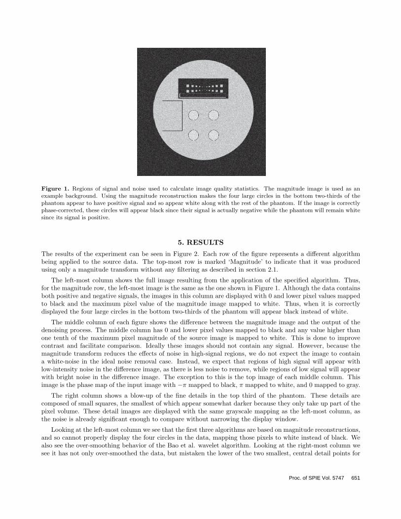
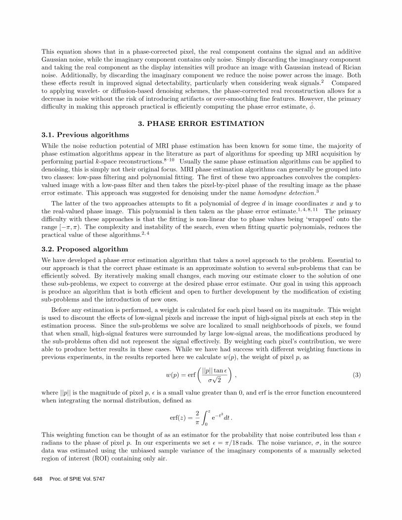
Figure 1. Regions of signal and noise used to calculate image quality statistics. The magnitude image is used as anexample background. Using the magnitude reconstruction makes the four large circles in the bottom two-thirds of thephantom appear to have positive signal and so appear white along with the rest of the phantom. If the image is correctlyphase-corrected, these circles will appear black since their signal is actually negative while the phantom will remain whitesince its signal is positive.

5. RESULTS

The results of the experiment can be seen in Figure 2. Each row of the figure represents a different algorithmbeing applied to the source data. The top-most row is marked ‘Magnitude’ to indicate that it was producedusing only a magnitude transform without any filtering as described in section 2.1.

The left-most column shows the full image resulting from the application of the specified algorithm. Thus,for the magnitude row, the left-most image is the same as the one shown in Figure 1. Although the data containsboth positive and negative signals, the images in this column are displayed with 0 and lower pixel values mappedto black and the maximum pixel value of the magnitude image mapped to white. Thus, when it is correctlydisplayed the four large circles in the bottom two-thirds of the phantom will appear black instead of white.

The middle column of each figure shows the difference between the magnitude image and the output of thedenoising process. The middle column has 0 and lower pixel values mapped to black and any value higher thanone tenth of the maximum pixel magnitude of the source image is mapped to white. This is done to improvecontrast and facilitate comparison. Ideally these images should not contain any signal. However, because themagnitude transform reduces the effects of noise in high-signal regions, we do not expect the image to containa white-noise in the ideal noise removal case. Instead, we expect that regions of high signal will appear withlow-intensity noise in the difference image, as there is less noise to remove, while regions of low signal will appearwith bright noise in the difference image. The exception to this is the top image of each middle column. Thisimage is the phase map of the input image with −π mapped to black, π mapped to white, and 0 mapped to gray.

The right column shows a blow-up of the fine details in the top third of the phantom. These details arecomposed of small squares, the smallest of which appear somewhat darker because they only take up part of thepixel volume. These detail images are displayed with the same grayscale mapping as the left-most column, asthe noise is already significant enough to compare without narrowing the display window.

Looking at the left-most column we see that the first three algorithms are based on magnitude reconstructions,and so cannot properly display the four circles in the data, mapping those pixels to white instead of black. Wealso see the over-smoothing behavior of the Bao et al. wavelet algorithm. Looking at the right-most column wesee it has not only over-smoothed the data, but mistaken the lower of the two smallest, central detail points for

Proc. of SPIE Vol. 5747 651

Magnitude

SNR: 14.63

CNR: 15.49

MSR: 14.63

Bao et al. Wavelet

SNR: 53.19

CNR: 82.09

MSR: 87.12

Nowak Rician Wavelet

SNR: 13.45

CNR: 16.75

MSR: 15.29

Proposed Phase Estimate

SNR: 15.52

CNR: 17.02

MSR: 14.56

Homodyne Phase Estimate

SNR: 15.16

CNR: 16.91

MSR: 14.55

Bernstein Phase Estimate

SNR: 15.11

CNR: 16.87

MSR: 14.56

Figure 2. Results from synthetic inversion recovery phantom image.

652 Proc. of SPIE Vol. 5747

noise an completely removed the detail. Nowak’s wavelet denoising scheme is more conservative and so has donea better job of retaining the fine points of the image while reducing the noise.

Of the three phase correction algorithms, we see that the homodyne detection algorithm has also failed toalign the negative signal in the correction direction. This is due to over-fitting of the phase estimate and sothe only solution for this image would be to reduce the number of Fourier coefficients retained in the homodynealgorithm’s filtering step. To explore this we ran the algorithm with several different filters and found that anysolution to under-fit the circles would in turn under-fit the fine points in the top third of the phantom, drowningthem out with the average phase of the surrounding noise. Our experiment confirms the statements by Noll thatthe homodyne algorithm will not necessarily work in cases with negative signal.3

The two algorithms that resulted in a correct display are the Bernstein polynomial fitting algorithm and ourproposed estimation approach. The success of the Bernstein polynomial fitting algorithm in the case can likely beattributed to the fact that the phase error was synthetically produced using the linear function in equation (4).Our synthetic example is the best-case scenario for the non-linear least squares fitting algorithm. Additionally, inthis experiment, the under-fitting was useful because it led to the correct error being estimated for the negativesignal regions as well. As noted by McGibney, this is not necessarily the case for polynomial fitting algorithmswhen large regions of the image consist of negative signal and a very poor fit may result instead.4

6. CONCLUSIONS AND DISCUSSION

We have presented a novel algorithm for performing phase error estimation in MRI images that is more com-putationally efficient than non-linear polynomial fitting. We have shown that the estimates produced by thealgorithm can be used as part of an image denoising scheme. We have also shown that, unlike homodyne de-tection, our proposed algorithm can be used to reconstruct inversion recovery images with regions of negativesignal.

Beyond the need for further validation of our algorithm, it is also important to determine which pulsesequences it can be applied to reliably. Our preliminary experiments on clinical data have shown our algorithmto be effective with spin echo and short-tau inversion recovery data. However, gradient-recalled echo and EPIimages have phase errors with many discontinuities and too high a curvature to be estimated using any of thephase estimation schemes discussed in this paper. More experiments on a variety of practical pulse sequencesare required in order to clarify the clinical value of our proposed algorithm.

Related to studying more pulse sequences, we mention in section 3.1 that phase error estimation is morefrequently discussed as a component of partial k-space MRI imaging. As our algorithm seems to have producedgood estimates using complete k-space data, we are interested to understand how it performs when given partialk-space data and if our algorithm’s estimates are useful in supporting partial k-space imaging.

We have yet to optimize our implementation and calculate the computation time required on representativesystems. One significant note though is that each of our proposed algorithm’s three sub-problems are designedso that each pixel can be calculated independently in any given step. Thus, while the output of any givensub-problem depends on the output of the sub-problem before, inside of a given sub-problem all the pixels areindependent of each other, relying only on pixels from the previous sub-problem. This independence meansthat our algorithm could be implemented using an efficient parallel setup. Implementations of this form will beconsidered when optimization begins.

Finally, the clear conflict between the calculated MSR, CNR, and SNR values and a visual assessment of theimage output indicates that these quality metrics should be used with caution. We are currently working toexplore other models that may allow for more medically significant measures of MRI image quality.

ACKNOWLEDGMENTS

The authors would like to thank Millennium Technology Inc. for providing data used in these experiments.Additionally, we would like to thank the Natural Science and Engineering Council of Canada and to SimonFraser University Industry Liaison Office for funding this research.

Proc. of SPIE Vol. 5747 653

REFERENCES1. C. B. Ahn and Z. H. Cho, “A new phase correction method in NMR imaging based on autocorrelation and

histogram analysis,” IEEE Transactions on Medical Imaging 6, pp. 32–36, March 1987.2. M. A. Bernstein, D. M. Thomasson, and W. Perman, “Improved detectability in low signal-to-noise ratio

magnetic resonance images by means of a phase-corrected real reconstruction,” Medical Physics 16, pp. 813–817, September 1989.

3. D. Noll, D. Nishimura, and A. Macovski, “Homodyne detection in magnetic resonance imaging,” IEEETransactions in Medical Imaging 10, pp. 154–163, 1991.

4. G. McGibney, “Phase sensitive reconstruction of MR images,” Master’s thesis, University of Calgary, 1991.5. H. Gudbjartsson and S. Patz, “The Rician distribution of noisy MRI data,” Magnetic Resonance in

Medicine 34, pp. 910–914, 1995.6. P. Bao and L. Zhang, “Noise reduction for magnetic resonance images via adaptive multiscale products

thresholding,” IEEE Transactions on Medical Imaging 22, pp. 1089–1099, September 2003.7. R. D. Nowak, “Wavelet-based Rician noise removal for magnetic resonance imaging,” Image Processing,

IEEE Transactions on 8, pp. 1408–1418, October 1999.8. J. R. MacFall, N. J. Pelc, and R. M. Vavrek, “Correction of spatially dependent phase shifts for partial

fourier imaging,” Magnetic Resonance Imaging 6(2), pp. 143–155, 1988.9. Z. P. Liang, F. E. Boada, R. T. Constable, E. M. Haacke, P. C. Lauterbur, and M. R. Smith, “Constrained

reconstruction methods in MR imaging,” Reviews of Magnetic Resonance in Medicine 4(67-185), 1992.10. G. McGibney, M. R. Smith, S. T. Nichols, and A. Crawley, “Quantitative evaluation of several partial fourier

reconstruction algorithms used in MRI,” Magnetic Resonance in Medicine 30, pp. 51–59, 1993.11. M. A. Bernstein and W. H. Perman, “Least-squares algorithm for phasing MR images,” in Book of Abstracts

vol. 2, Sixth Annual Meeting of SMRM, p. 801, Society of Magnetic Resonance in Medicine, August 1987.12. Wolfram Research, Inc., “Mathematica v5.0,” 2003.13. M. J. Firbank, A. Coulthard, R. M. Harrison, and E. D. Williams, “A comparison of two methods for

measuring the signal to noise ratio on MR images,” Phys. Med. Biology 44, pp. 261–264, 1999.

654 Proc. of SPIE Vol. 5747