Mr. Vincenzo Capuano Dr. Cyril Botteron Prof. Pierre-André ... · Mr. Vincenzo Capuano École Polytechnique Fédérale de Lausanne (ESPLAB), Switzerland, [email protected]

64th International Astronautical Congress, Beijing, China. Copyright ©2013 by the International Astronautical Federation. All rights reserved.

IAC-13- B2.1.3 Page 1 of 15

IAC-13-B2.1.3

GNSS PERFORMANCES FOR MEO, GEO AND HEO

Mr. Vincenzo Capuano École Polytechnique Fédérale de Lausanne (ESPLAB), Switzerland, [email protected]

Dr. Cyril Botteron

École Polytechnique Fédérale de Lausanne (ESPLAB), Switzerland, [email protected]

Prof. Pierre-André Farine École Polytechnique Fédérale de Lausanne (ESPLAB), Switzerland, [email protected]

Global Navigation Satellite Systems (GNSSs) such as GPS, GLONASS, and the future Galileo and BeiDou, have

demonstrated to be a valid and efficient system for various space applications in Low Earth Orbit (LEO), such as spacecraft orbit and attitude determination, rendezvous and formation flight of two or more spacecrafts, and timing synchronization. A GNSS presents a number of significant advantages, in particular for small satellites: it provides an autonomous navigation system, which requires just a relatively inexpensive realization and installation cost of the on board GNSS receiver, with low power consumption, limited mass and volume. Nowadays, the GNSS technology for LEO satellites is often used, thanks to the large number of visible satellites, the good geometry coverage and the strong signal power. However, the research of GNSS solutions for Medium Earth Orbit (MEO), Geostationary Earth Orbit (GEO) and High Earth Orbit (HEO) satellites is still new. In this context, this study aims to estimate accurately the GPS and Galileo performances for MEO, GEO and HEO use, such as for lunar applications. Unlike most of the previous investigations, our study is making use of a very accurate multi-GNSS full constellation simulator “Spirent GSS8000", which supports simultaneously the GPS and Galileo systems and the L1, L5, E1, E5 frequency bands. Performances offered by GPS and by GPS-Galileo-combined systems are evaluated in terms of availability, pseudorange error factors, geometry factors, Doppler shifts and Doppler rates.

I. INTRODUCTION Although primarily conceived as military navigation

systems for land, sea and airborne users, nowadays Global Navigation Satellite Systems (GNSSs) such as GPS, GLONASS, and the future Galileo and BeiDou, can also be considered as effective and efficient systems for a considerable number of space applications. These include autonomous real time spacecraft position and attitude determination, precise orbit determination, rendezvous, formation flight of two or more spacecraft and timing synchronization [1]. Moreover, a GNSS seems to be suitable for small satellites, because it requires relatively inexpensive realization and installation cost of the on-board GNSS receiver, which has low power consumption, limited mass and volume, and provides an autonomous navigation system. Projections show that over the next twenty years approximately [2]: 60% of space missions will operate in LEO (which ranges from an altitude of 100 km to about 2000 km), 35% of space missions will operate at higher altitudes up to GEO (altitude of approximately 36 000 km) and the rest will be a Cislunar / Interplanetary or HEO missions. Today, thanks to the large number of visible satellites, the good geometry coverage and the strong signal power, many GNSS receivers are already successfully flying on satellites in LEO orbits. In fact, most LEO space users

share similar operational benefits as more “traditional” Earth users. However, space remains a challenging operational environment at higher altitudes, such as MEO, GEO and HEO, where the GNSS receiver performance and the GNSS solution (e.g. navigation solution) are considerably affected. The receiver performances are in fact strongly influenced by high spacecraft translational and rotational dynamics, weaker received signals power, thermo-mechanical stresses and possible multipath effects, self-induced from the nearby surfaces or due to reflection with other vehicles. Moreover, the GNSS solution may not even exist if a minimum number of GNSS satellites are not in the line of sight (LOS) or of course if the GNSS receiver is not able to acquire their signals. If a GNSS solution exists, i.e. for code-based observations, its error will depend on the product between a geometry factor (the composite effect of the relative satellite-user geometry on the GNSS solution error) and a pseudorange error factor (a statistical sum of the contributions from each of the ranging error sources) [3]. In particular, the higher will be the orbit above the GNSS constellation, the larger will be the geometry error factor and accordingly the larger will be the GNSS solution error.

The aim of this paper is to estimate accurately the GPS and GPS-Galileo-combined performances for MEO, GEO and HEO use, such as for lunar transfer


IAC-13- B2.1.3 Page 2 of 15

trajectories, in terms of availability, pseudorange error factors and geometry factors. Furthermore, the Doppler shift and the Doppler rate are calculated for the considered orbital cases, being an influential parameter in the GNSS receiver design. Unlike most of the previous investigations, this study is making use of the very accurate multi-GNSS constellation simulator “Spirent GSS8000", which supports simultaneously the GPS and Galileo systems and the L1, L5, E1, E5 frequency bands. Spirent simulator includes facilities to accommodate to the special needs of space-based receiver testing, including [4]: � Full account for the double atmosphere effect of

signals passing through the atmosphere twice for the GNSS satellites located on the far side of the Earth.

� Realistic satellite transmit-antenna patterns. � Spacecraft models and spacecraft motion models. � Ability to define trajectory data, including in real-

time.

II. SIMULATION MODELS AND ASSUMPTIONS

As already mentioned, the GNSS performances are evaluated for the GPS constellation and for the GPS-Galileo-combined constellation. The initial time of the performed simulations is arbitrarily selected as February 13, 2013, 0:00:00 UTC. II.I Atmosphere Model

The areas of the atmosphere, known as the ionosphere and the troposphere, delay the RF signal from each GNSS satellite to the receiver. In order to calculate the true range from each satellite, and hence the receiver position, these delays must be taken into account [5]. To calculate the tropospheric delay, the simulator uses the tropospheric model from reference [6]. Regarding the ionospheric delay, for Galileo satellites, it uses the NeQuick ionospheric model described in [5] and [7], which applies equally well to both terrestrial and space-borne receivers. For GPS satellites, the ionospheric delay is modelled according to the Klobuchar model [8]. Furthermore, because the Klobuchar model is not applicable at altitudes within, or above, the ionosphere, the simulator switches for altitudes above 80 km between the Klobuchar model and an alternative one, defined in [5], which takes into account the reduction in the ionization level (Total Electron Count, or TEC) with increasing height in the ionospheric layer. II.II Constellations Model

The constellations model consists of 31 GPS satellites, including at least four satellites in each of six orbital planes, as described in [8], and 27 Galileo satellites as in the “standard” Galileo constellation defined in [9].

II.III Signals Model In this study just the L1 GPS and E1 Galileo

frequencies are considered, for which it is assumed respectively a power reference level of -130 dBm and of -125.5 dBm. Each satellite signal strength is modelled to provide realistic signal levels at the receiver position �� by using the following formula from [5]:

�� [1]

where :

�� is the guaranteed minimum signal level for the GNSS satellite, here assumed -130 dBm for GPS and -125.5 dBm for Galileo.

� “Global Offset”. In Spirent simulator, the default value is 10 dB for both constellations [5]. This value is chosen to match the performance obtained when using the simulator with the performance obtained when using a real antenna capturing a real signal under good conditions (i.e., a clear view of the sky). More specifically, part of this offset results from the higher transmit power of the satellites as compared to the minimum signal specifications, and part compensates for the higher thermal noise floor in the simulations than as captured by a real antenna pointing to the sky (i.e., the real antenna temperature is typically much lower than the ambient temperature).

�� is the reference range used for inverse-square variation calculation and equal to the range from a receiver to the GNSS satellite at zero elevation. �� !�"#$% &$%��'(&$�'#)&*" + � �%#'$,�'#)&*" +

� is the range from GNSS satellite to the receiver.

�� is the loss from the GNSS satellite transmit antenna in the direction of the receiver.

�� is the loss from the receiver antenna in the direction of the GNSS satellite.

II.IV Transmitter Antenna Patterns

The transmitter antenna level pattern is modeled to simulate the directional (angular) dependence of the strength of the radio waves from the GNSS transmitter antenna. Since the GNSS transmitter antenna points to the Earth (the antenna main lobe is directed to the Earth, to serve the Earth user), this has a significant effect for


IAC-13- B2.1.3 Page 3 of 15

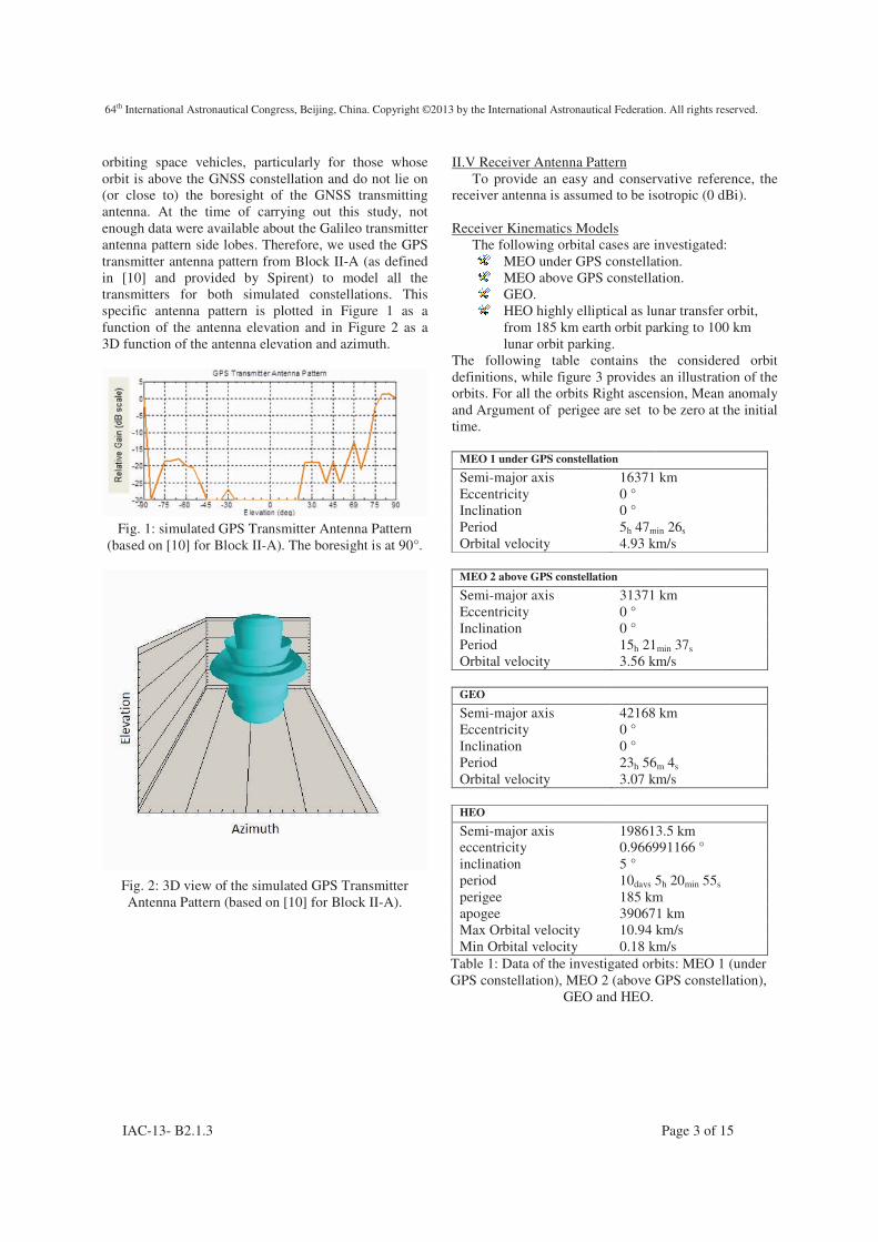
orbiting space vehicles, particularly for those whose orbit is above the GNSS constellation and do not lie on (or close to) the boresight of the GNSS transmitting antenna. At the time of carrying out this study, not enough data were available about the Galileo transmitter antenna pattern side lobes. Therefore, we used the GPS transmitter antenna pattern from Block II-A (as defined in [10] and provided by Spirent) to model all the transmitters for both simulated constellations. This specific antenna pattern is plotted in Figure 1 as a function of the antenna elevation and in Figure 2 as a 3D function of the antenna elevation and azimuth.

Fig. 1: simulated GPS Transmitter Antenna Pattern

(based on [10] for Block II-A). The boresight is at 90°.

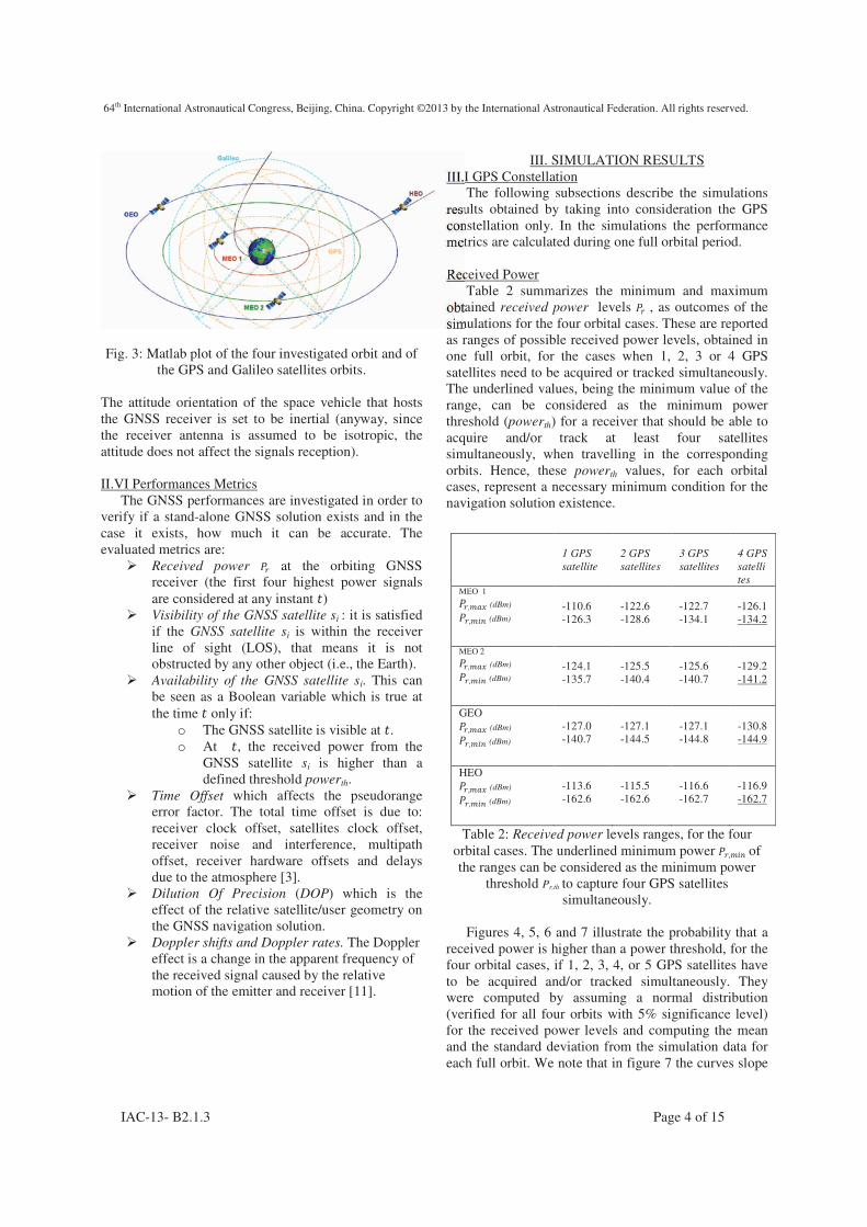
Fig. 2: 3D view of the simulated GPS Transmitter Antenna Pattern (based on [10] for Block II-A).

II.V Receiver Antenna Pattern To provide an easy and conservative reference, the

receiver antenna is assumed to be isotropic (0 dBi). Receiver Kinematics Models

The following orbital cases are investigated: MEO under GPS constellation. MEO above GPS constellation. GEO. HEO highly elliptical as lunar transfer orbit,

from 185 km earth orbit parking to 100 km lunar orbit parking.

The following table contains the considered orbit definitions, while figure 3 provides an illustration of the orbits. For all the orbits Right ascension, Mean anomaly and Argument of perigee are set to be zero at the initial time.

MEO 1 under GPS constellation Semi-major axis 16371 km Eccentricity 0 ° Inclination 0 ° Period 5h 47min 26s Orbital velocity 4.93 km/s

MEO 2 above GPS constellation Semi-major axis 31371 km Eccentricity 0 ° Inclination 0 ° Period 15h 21min 37s Orbital velocity 3.56 km/s

GEO Semi-major axis 42168 km Eccentricity 0 ° Inclination 0 ° Period 23h 56m 4s Orbital velocity 3.07 km/s

HEO Semi-major axis 198613.5 km eccentricity 0.966991166 ° inclination 5 ° period 10days 5h 20min 55s perigee 185 km apogee 390671 km Max Orbital velocity 10.94 km/s Min Orbital velocity 0.18 km/s

Table 1: Data of the investigated orbits: MEO 1 (under GPS constellation), MEO 2 (above GPS constellation),

GEO and HEO.


IAC-13- B2.1.3 Page 4 of 15

Fig. 3: Matlab plot of the four investigated orbit and of the GPS and Galileo satellites orbits.

The attitude orientation of the space vehicle that hosts the GNSS receiver is set to be inertial (anyway, since the receiver antenna is assumed to be isotropic, the attitude does not affect the signals reception). II.VI Performances Metrics

The GNSS performances are investigated in order to verify if a stand-alone GNSS solution exists and in the case it exists, how much it can be accurate. The evaluated metrics are:

� Received power �� at the orbiting GNSS receiver (the first four highest power signals are considered at any instant $)

� Visibility of the GNSS satellite si : it is satisfied if the GNSS satellite si is within the receiver line of sight (LOS), that means it is not obstructed by any other object (i.e., the Earth).

� Availability of the GNSS satellite si. This can be seen as a Boolean variable which is true at the time $ only if:

o The GNSS satellite is visible at $. o At $, the received power from the

GNSS satellite si is higher than a defined threshold powerth.

� Time Offset which affects the pseudorange error factor. The total time offset is due to: receiver clock offset, satellites clock offset, receiver noise and interference, multipath offset, receiver hardware offsets and delays due to the atmosphere [3].

� Dilution Of Precision (DOP) which is the effect of the relative satellite/user geometry on the GNSS navigation solution.

� Doppler shifts and Doppler rates. The Doppler effect is a change in the apparent frequency of the received signal caused by the relative motion of the emitter and receiver [11].

III. SIMULATION RESULTS III.I GPS Constellation

The following subsections describe the simulations results obtained by taking into consideration the GPS constellation only. In the simulations the performance metrics are calculated during one full orbital period. Received Power

Table 2 summarizes the minimum and maximum obtained received power levels �� , as outcomes of the simulations for the four orbital cases. These are reported as ranges of possible received power levels, obtained in one full orbit, for the cases when 1, 2, 3 or 4 GPS satellites need to be acquired or tracked simultaneously. The underlined values, being the minimum value of the range, can be considered as the minimum power threshold (powerth) for a receiver that should be able to acquire and/or track at least four satellites simultaneously, when travelling in the corresponding orbits. Hence, these powerth values, for each orbital cases, represent a necessary minimum condition for the navigation solution existence.

Table 2: Received power levels ranges, for the four orbital cases. The underlined minimum power ��-�./ of the ranges can be considered as the minimum power

threshold Pr,th to capture four GPS satellites simultaneously.

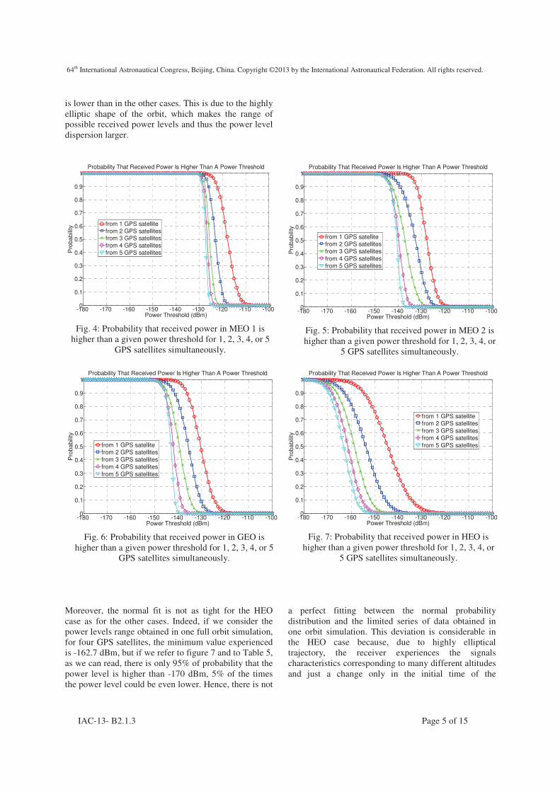
Figures 4, 5, 6 and 7 illustrate the probability that a

received power is higher than a power threshold, for the four orbital cases, if 1, 2, 3, 4, or 5 GPS satellites have to be acquired and/or tracked simultaneously. They were computed by assuming a normal distribution (verified for all four orbits with 5% significance level) for the received power levels and computing the mean and the standard deviation from the simulation data for each full orbit. We note that in figure 7 the curves slope

1 GPS

satellite

2 GPS

satellites

3 GPS

satellites

4 GPS

satelli

tes MEO 1

��-�01 (dBm)

��-�./ (dBm)

-110.6 -126.3

-122.6 -128.6

-122.7 -134.1

-126.1 -134.2

MEO 2

��-�01 (dBm)

��-�./ (dBm)

-124.1 -135.7

-125.5 -140.4

-125.6 -140.7

-129.2 -141.2

GEO ��-�01 (dBm)

��-�./ (dBm)

-127.0 -140.7

-127.1 -144.5

-127.1 -144.8

-130.8 -144.9

HEO ��-�01 (dBm)

��-�./ (dBm)

-113.6 -162.6

-115.5 -162.6

-116.6 -162.7

-116.9 -162.7


IAC-13- B2.1.3 Page 5 of 15

is lower than in the other cases. This is due to the highly elliptic shape of the orbit, which makes the range of possible received power levels and thus the power level dispersion larger.

Fig. 4: Probability that received power in MEO 1 is higher than a given power threshold for 1, 2, 3, 4, or 5

GPS satellites simultaneously.

Fig. 5: Probability that received power in MEO 2 is higher than a given power threshold for 1, 2, 3, 4, or

5 GPS satellites simultaneously.

Fig. 6: Probability that received power in GEO is higher than a given power threshold for 1, 2, 3, 4, or 5

GPS satellites simultaneously.

Fig. 7: Probability that received power in HEO is higher than a given power threshold for 1, 2, 3, 4, or

5 GPS satellites simultaneously.

Moreover, the normal fit is not as tight for the HEO case as for the other cases. Indeed, if we consider the power levels range obtained in one full orbit simulation, for four GPS satellites, the minimum value experienced is -162.7 dBm, but if we refer to figure 7 and to Table 5, as we can read, there is only 95% of probability that the power level is higher than -170 dBm, 5% of the times the power level could be even lower. Hence, there is not

a perfect fitting between the normal probability distribution and the limited series of data obtained in one orbit simulation. This deviation is considerable in the HEO case because, due to highly elliptical trajectory, the receiver experiences the signals characteristics corresponding to many different altitudes and just a change only in the initial time of the

-180 -170 -160 -150 -140 -130 -120 -110 -1000

0.1

0.2

0.3

0.4

0.5

0.6

0.7

0.8

0.9

1

Power Threshold (dBm)

Pro

bab

ility

Probability That Received Power Is Higher Than A Power Threshold

from 1 GPS satellite

from 2 GPS satellitesfrom 3 GPS satellites

from 4 GPS satellites


-180 -170 -160 -150 -140 -130 -120 -110 -1000

0.1

0.2

0.3

0.4

0.5

0.6

0.7

0.8

0.9

1


Pro

bab

ility


from 1 GPS satellitefrom 2 GPS satellitesfrom 3 GPS satellites


-180 -170 -160 -150 -140 -130 -120 -110 -1000

0.1

0.2

0.3

0.4

0.5

0.6

0.7

0.8

0.9

1


Pro

ba

bili

ty


from 1 GPS satellitefrom 2 GPS satellites



-180 -170 -160 -150 -140 -130 -120 -110 -1000

0.1

0.2

0.3

0.4

0.5

0.6

0.7

0.8

0.9

1


Pro

ba

bili

ty


from 1 GPS satellitefrom 2 GPS satellites




IAC-13- B2.1.3 Page 6 of 15

performed simulation would change the power levels range. Visibility and Availability

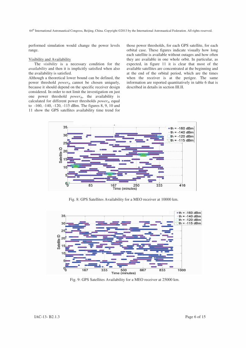
The visibility is a necessary condition for the availability and then it is implicitly satisfied when also the availability is satisfied. Although a theoretical lower bound can be defined, the power threshold powerth cannot be chosen uniquely, because it should depend on the specific receiver design considered. In order to not limit the investigation on just one power threshold powerth, the availability is calculated for different power thresholds powerth equal to -160, -140, -120, -115 dBm. The figures 8, 9, 10 and 11 show the GPS satellites availability time trend for

those power thresholds, for each GPS satellite, for each orbital case. These figures indicate visually how long each satellite is available without outages and how often they are available in one whole orbit. In particular, as expected, in figure 11 it is clear that most of the available satellites are concentrated at the beginning and at the end of the orbital period, which are the times when the receiver is at the perigee. The same information are reported quantitatively in table 6 that is described in details in section III.II.

Fig. 8: GPS Satellites Availability for a MEO receiver at 10000 km.

Fig. 9: GPS Satellites Availability for a MEO receiver at 25000 km.


IAC-13- B2.1.3 Page 7 of 15

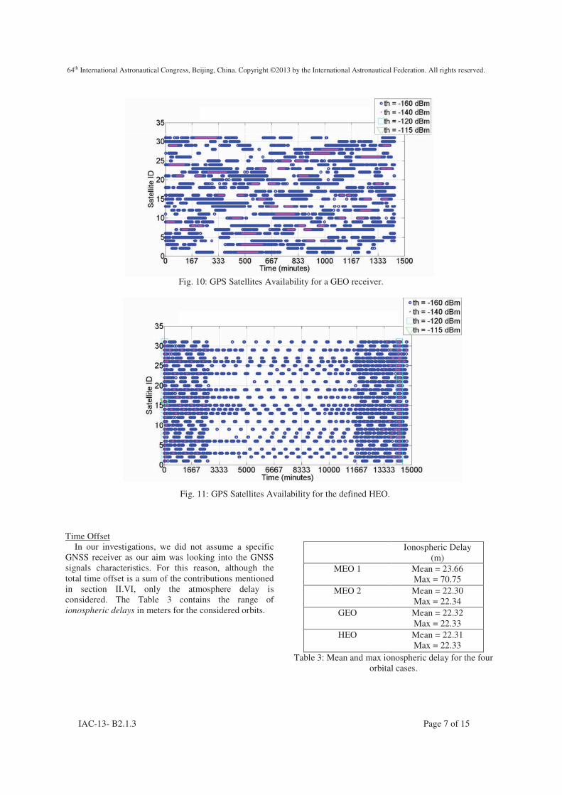
Fig. 10: GPS Satellites Availability for a GEO receiver.

Fig. 11: GPS Satellites Availability for the defined HEO.

Time Offset In our investigations, we did not assume a specific GNSS receiver as our aim was looking into the GNSS signals characteristics. For this reason, although the total time offset is a sum of the contributions mentioned in section II.VI, only the atmosphere delay is considered. The Table 3 contains the range of ionospheric delays in meters for the considered orbits.

Ionospheric Delay (m)

MEO 1 Mean = 23.66 Max = 70.75

MEO 2 Mean = 22.30 Max = 22.34

GEO Mean = 22.32 Max = 22.33

HEO Mean = 22.31 Max = 22.33

Table 3: Mean and max ionospheric delay for the four orbital cases.


IAC-13- B2.1.3 Page 8 of 15

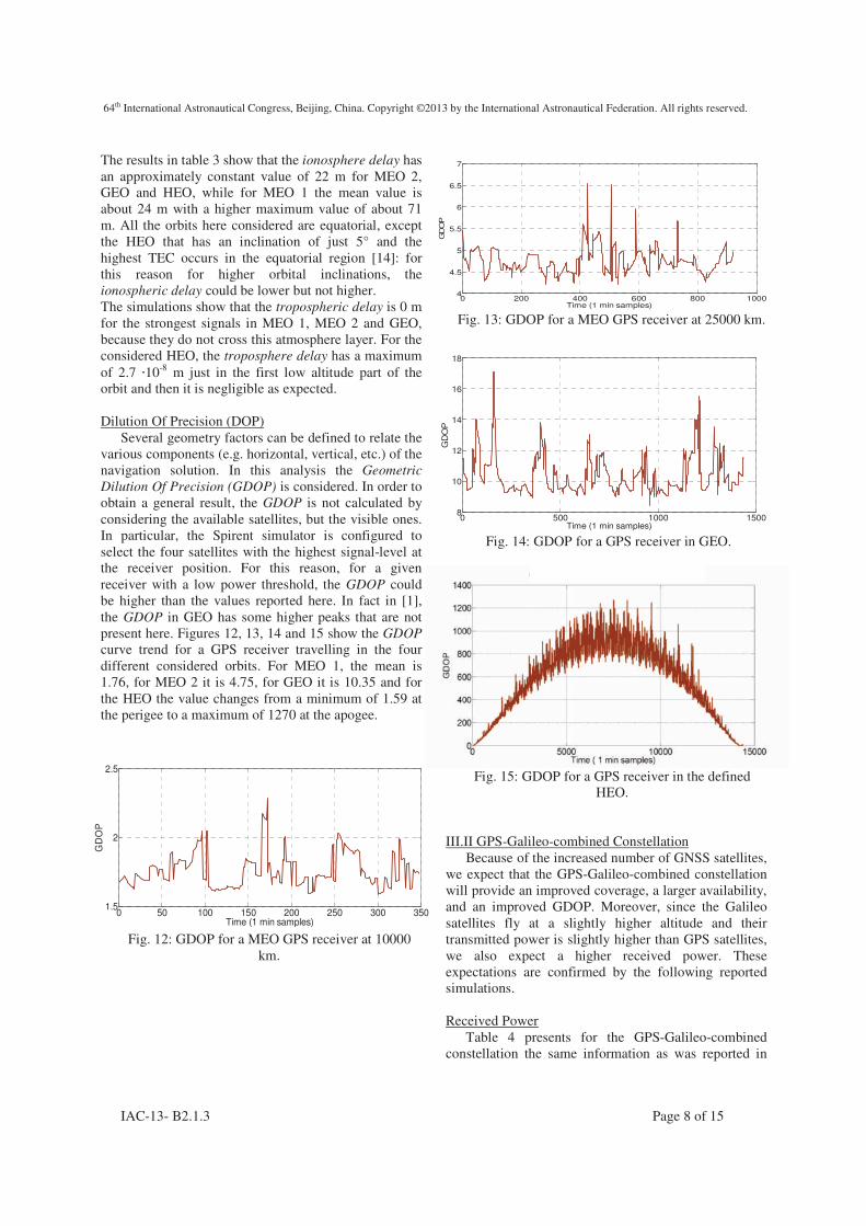
The results in table 3 show that the ionosphere delay has an approximately constant value of 22 m for MEO 2, GEO and HEO, while for MEO 1 the mean value is about 24 m with a higher maximum value of about 71 m. All the orbits here considered are equatorial, except the HEO that has an inclination of just 5° and the highest TEC occurs in the equatorial region [14]: for this reason for higher orbital inclinations, the ionospheric delay could be lower but not higher. The simulations show that the tropospheric delay is 0 m for the strongest signals in MEO 1, MEO 2 and GEO, because they do not cross this atmosphere layer. For the considered HEO, the troposphere delay has a maximum of 2.7 210-8 m just in the first low altitude part of the orbit and then it is negligible as expected. Dilution Of Precision (DOP)

Several geometry factors can be defined to relate the various components (e.g. horizontal, vertical, etc.) of the navigation solution. In this analysis the Geometric

Dilution Of Precision (GDOP) is considered. In order to obtain a general result, the GDOP is not calculated by considering the available satellites, but the visible ones. In particular, the Spirent simulator is configured to select the four satellites with the highest signal-level at the receiver position. For this reason, for a given receiver with a low power threshold, the GDOP could be higher than the values reported here. In fact in [1], the GDOP in GEO has some higher peaks that are not present here. Figures 12, 13, 14 and 15 show the GDOP curve trend for a GPS receiver travelling in the four different considered orbits. For MEO 1, the mean is 1.76, for MEO 2 it is 4.75, for GEO it is 10.35 and for the HEO the value changes from a minimum of 1.59 at the perigee to a maximum of 1270 at the apogee.

Fig. 12: GDOP for a MEO GPS receiver at 10000 km.

Fig. 13: GDOP for a MEO GPS receiver at 25000 km.

Fig. 14: GDOP for a GPS receiver in GEO.

Fig. 15: GDOP for a GPS receiver in the defined HEO.

III.II GPS-Galileo-combined Constellation

Because of the increased number of GNSS satellites, we expect that the GPS-Galileo-combined constellation will provide an improved coverage, a larger availability, and an improved GDOP. Moreover, since the Galileo satellites fly at a slightly higher altitude and their transmitted power is slightly higher than GPS satellites, we also expect a higher received power. These expectations are confirmed by the following reported simulations. Received Power

Table 4 presents for the GPS-Galileo-combined constellation the same information as was reported in

0 50 100 150 200 250 300 3501.5

2

2.5

Time (1 min samples)

GD

OP

GDOP For A MEO GPS Receiver At 10000 Km

0 200 400 600 800 10004

4.5

5

5.5

6

6.5

7


GD

OP

GDOP For A MEO GPS Receiver At 25000 Km

0 500 1000 15008

10

12

14

16

18


GD

OP

GDOP For A GPS Receiver In GEO


IAC-13- B2.1.3 Page 9 of 15

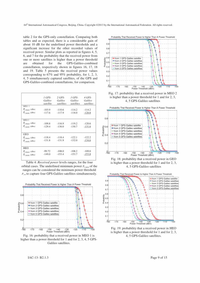
table 2 for the GPS-only constellation. Comparing both tables and as expected, there is a considerable gain of about 10 dB for the underlined power thresholds and a significant increase for the other recorded values of received power. Similar plots as reported in figures 4, 5, 6, and 7 for the probability that the received power from one or more satellites is higher than a power threshold are obtained for the GPS-Galileo-combined constellation, respectively shown in figures 16, 17, 18 and 19. Table 5 presents the received power values corresponding to 67% and 95% probability, for 1, 2, 3, 4, 5 simultaneously captured satellites, of the GPS and GPS-Galileo-combined constellations, for comparison.

Table 4: Received power levels ranges, for the four orbital cases. The underlined minimum power ��-�./ of the ranges can be considered the minimum power threshold

Pr,th to capture four GPS-Galileo satellites simultaneously.

Fig. 16: probability that a received power in MEO 1 is higher than a power threshold for 1 and for 2, 3, 4, 5 GPS-

Galileo satellites.

Fig. 17: probability that a received power in MEO 2 is higher than a power threshold for 1 and for 2, 3,

4, 5 GPS-Galileo satellites

Fig. 18: probability that a received power in GEO is higher than a power threshold for 1 and for 2, 3,

4, 5 GPS-Galileo satellites

Fig. 19: probability that a received power in HEO is higher than a power threshold for 1 and for 2, 3,

4, 5 GPS-Galileo satellites.

-180 -170 -160 -150 -140 -130 -120 -110 -1000

0.2

0.4

0.6

0.8

1


Pro

ba

bili

ty


from 1 GPS-Galileo satellite

from 2 GPS-Galileo satellitesfrom 3 GPS-Galileo satellites

from 4 GPS-Galileo satellites


-180 -170 -160 -150 -140 -130 -120 -110 -1000

0.1

0.2

0.3

0.4

0.5

0.6

0.7

0.8

0.9

1


Pro

babili

ty


from 1 GPS-Galileo satellite





-180 -170 -160 -150 -140 -130 -120 -110 -1000

0.2

0.4

0.6

0.8

1


Pro

ba

bili

ty


from 1 GPS-Galileo satellitefrom 2 GPS-Galileo satellites




-180 -170 -160 -150 -140 -130 -120 -110 -1000

0.1

0.2

0.3

0.4

0.5

0.6

0.7

0.8

0.9

1


�P

robabili

ty

Probability That Received Power Is Higher Then A Power Threshold

from 1 GPS-Galileo satellitefrom 2 GPS-Galileo satellites




1 GPS-

Galileo

satellite

2 GPS-

Galileo

satellites

3 GPS-

Galileo

satellites

4 GPS-

Galileo

satellites MEO 1

��-�01 (dBm)

��-�./ (dBm)

-103.9 -117.6

-110.6 -117.9

-114.2 -118.0

-114.2 -120.8

MEO 2

��-�01 (dBm)

��-�./ (dBm)

-109.8 -129.4

-116.9 -130.0

-119.2 -130.7

-120.6 -131.6

GEO ��-�01 (dBm)

��-�./ (dBm)

-118.4 -131.8

-118.4 -131.9

-122.1 -132.0

-122.2 -134.6

HEO ��-�01 (dBm)

��-�./ (dBm)

-99.72 -149.0

-108.0 -153.4

-108.2 -153.7

-109.0 -153.8


IAC-13- B2.1.3 Page 10 of 15

Number of satellites

simultaneously captured

Percentile Received power (dBm) MEO 1

Received power (dBm) MEO 2

Received power (dBm) GEO

Received power (dBm) HEO

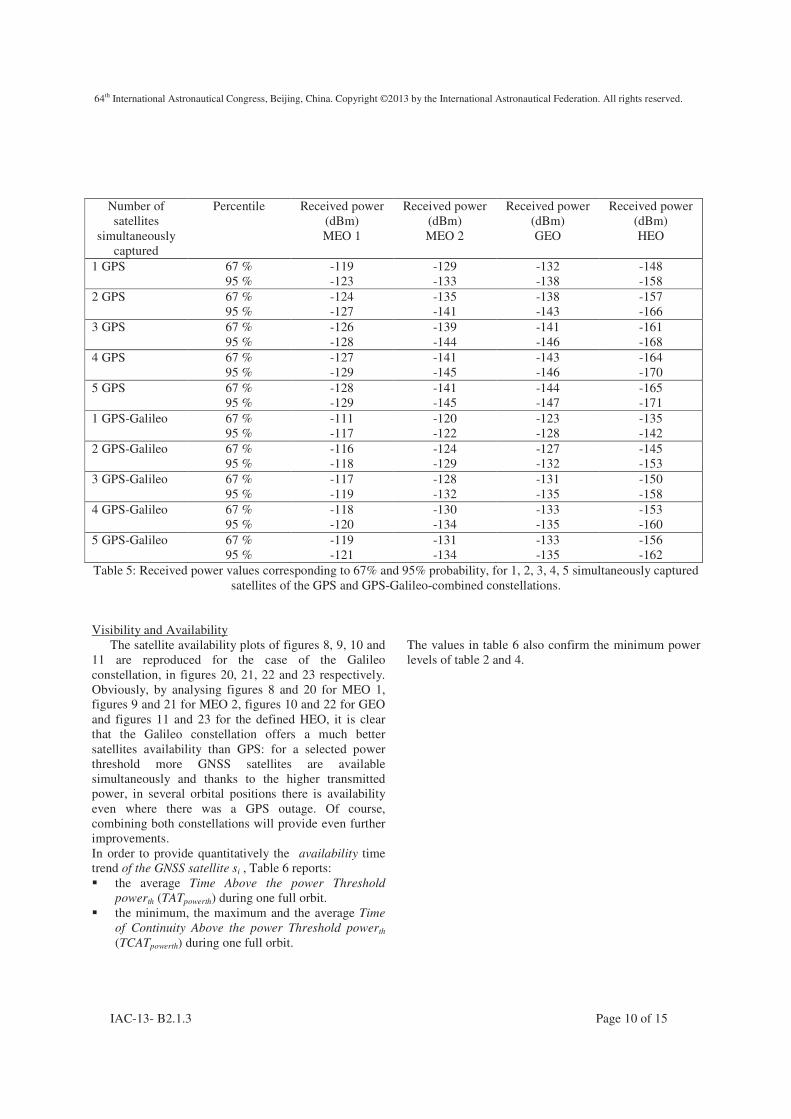
1 GPS 67 % -119 -129 -132 -148 95 % -123 -133 -138 -158 2 GPS 67 % -124 -135 -138 -157 95 % -127 -141 -143 -166 3 GPS 67 % -126 -139 -141 -161 95 % -128 -144 -146 -168 4 GPS 67 % -127 -141 -143 -164 95 % -129 -145 -146 -170 5 GPS 67 % -128 -141 -144 -165 95 % -129 -145 -147 -171 1 GPS-Galileo 67 % -111 -120 -123 -135 95 % -117 -122 -128 -142 2 GPS-Galileo 67 % -116 -124 -127 -145 95 % -118 -129 -132 -153 3 GPS-Galileo 67 % -117 -128 -131 -150 95 % -119 -132 -135 -158 4 GPS-Galileo 67 % -118 -130 -133 -153 95 % -120 -134 -135 -160 5 GPS-Galileo 67 % -119 -131 -133 -156 95 % -121 -134 -135 -162 Table 5: Received power values corresponding to 67% and 95% probability, for 1, 2, 3, 4, 5 simultaneously captured

satellites of the GPS and GPS-Galileo-combined constellations. Visibility and Availability

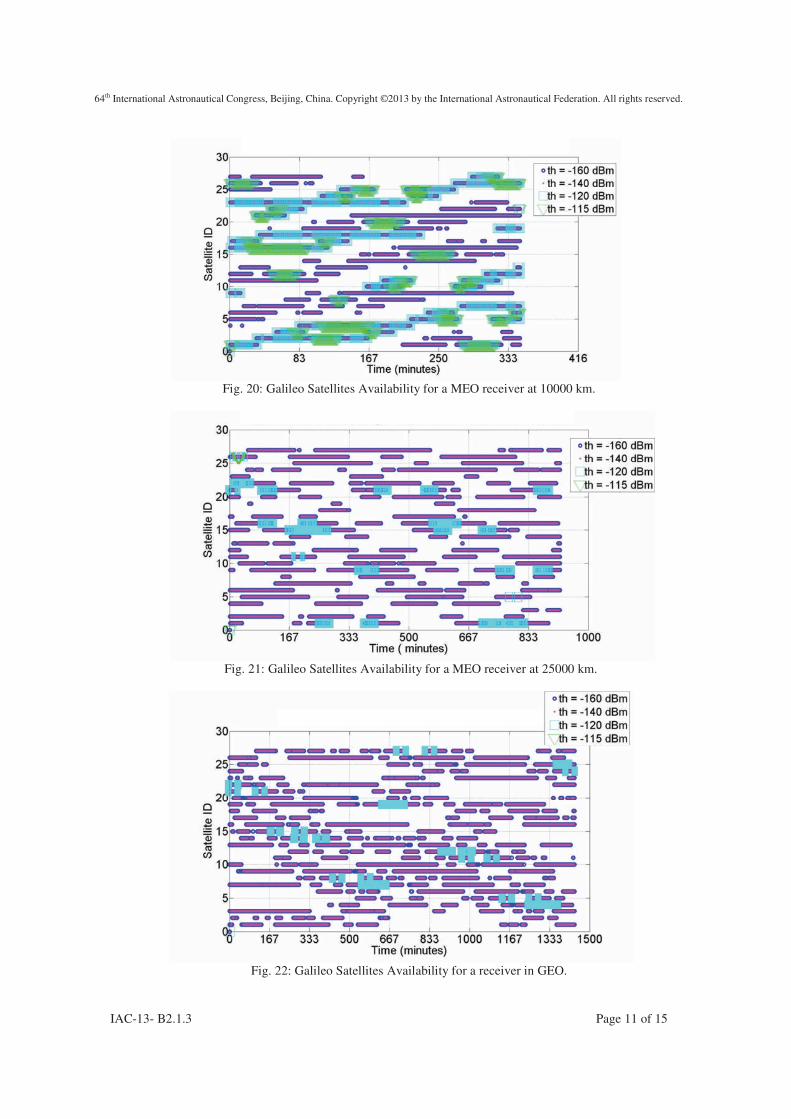
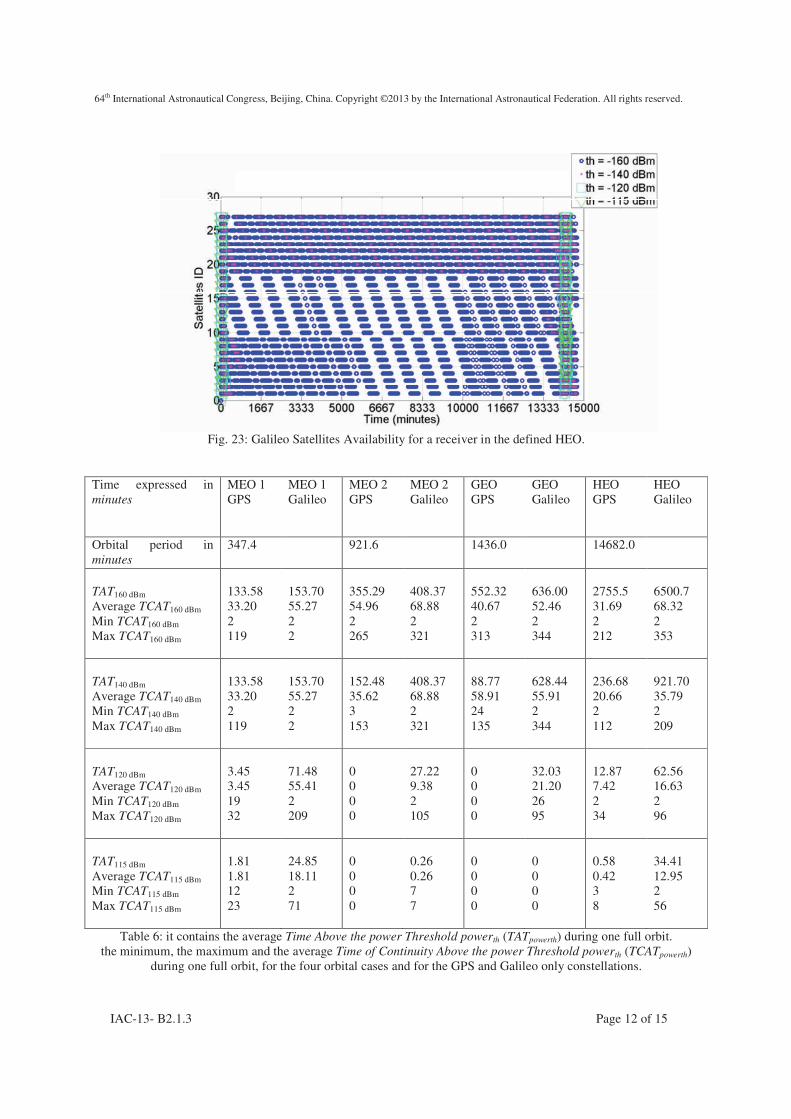
The satellite availability plots of figures 8, 9, 10 and 11 are reproduced for the case of the Galileo constellation, in figures 20, 21, 22 and 23 respectively. Obviously, by analysing figures 8 and 20 for MEO 1, figures 9 and 21 for MEO 2, figures 10 and 22 for GEO and figures 11 and 23 for the defined HEO, it is clear that the Galileo constellation offers a much better satellites availability than GPS: for a selected power threshold more GNSS satellites are available simultaneously and thanks to the higher transmitted power, in several orbital positions there is availability even where there was a GPS outage. Of course, combining both constellations will provide even further improvements. In order to provide quantitatively the availability time trend of the GNSS satellite si , Table 6 reports: � the average Time Above the power Threshold

powerth (TATpowerth) during one full orbit. � the minimum, the maximum and the average Time

of Continuity Above the power Threshold powerth (TCATpowerth) during one full orbit.

The values in table 6 also confirm the minimum power levels of table 2 and 4.


IAC-13- B2.1.3 Page 11 of 15

Fig. 20: Galileo Satellites Availability for a MEO receiver at 10000 km.

Fig. 21: Galileo Satellites Availability for a MEO receiver at 25000 km.

Fig. 22: Galileo Satellites Availability for a receiver in GEO.


IAC-13- B2.1.3 Page 12 of 15

Fig. 23: Galileo Satellites Availability for a receiver in the defined HEO.

Time expressed in minutes

MEO 1 GPS

MEO 1 Galileo

MEO 2 GPS

MEO 2 Galileo

GEO GPS

GEO Galileo

HEO GPS

HEO Galileo

Orbital period in minutes

347.4 921.6 1436.0 14682.0

TAT160 dBm

Average TCAT160 dBm

Min TCAT160 dBm

Max TCAT160 dBm

133.58 33.20 2 119

153.70 55.27 2 2

355.29 54.96 2 265

408.37 68.88 2 321

552.32 40.67 2 313

636.00 52.46 2 344

2755.5 31.69 2 212

6500.7 68.32 2 353

TAT140 dBm

Average TCAT140 dBm

Min TCAT140 dBm

Max TCAT140 dBm

133.58 33.20 2 119

153.70 55.27 2 2

152.48 35.62 3 153

408.37 68.88 2 321

88.77 58.91 24 135

628.44 55.91 2 344

236.68 20.66 2 112

921.70 35.79 2 209

TAT120 dBm

Average TCAT120 dBm

Min TCAT120 dBm

Max TCAT120 dBm

3.45 3.45 19 32

71.48 55.41 2 209

0 0 0 0

27.22 9.38 2 105

0 0 0 0

32.03 21.20 26 95

12.87 7.42 2 34

62.56 16.63 2 96

TAT115 dBm

Average TCAT115 dBm

Min TCAT115 dBm

Max TCAT115 dBm

1.81 1.81 12 23

24.85 18.11 2 71

0 0 0 0

0.26 0.26 7 7

0 0 0 0

0 0 0 0

0.58 0.42 3 8

34.41 12.95 2 56

Table 6: it contains the average Time Above the power Threshold powerth (TATpowerth) during one full orbit. the minimum, the maximum and the average Time of Continuity Above the power Threshold powerth (TCATpowerth)

during one full orbit, for the four orbital cases and for the GPS and Galileo only constellations.


IAC-13- B2.1.3 Page 13 of 15

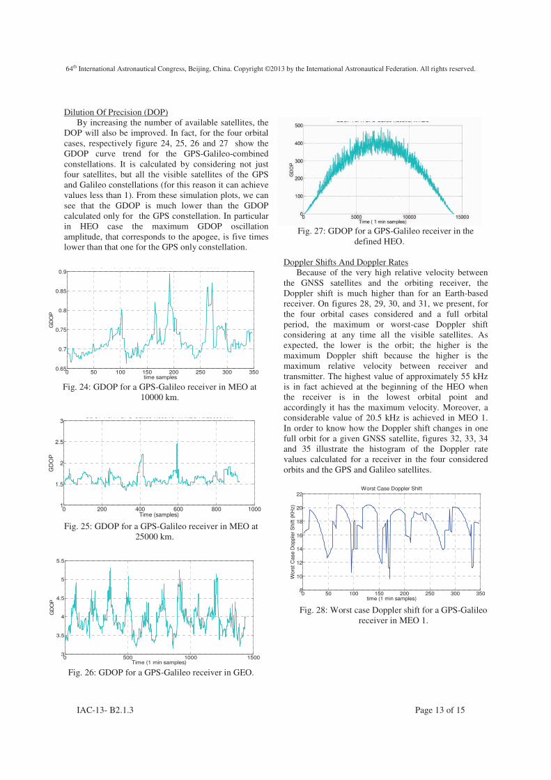
Dilution Of Precision (DOP)

By increasing the number of available satellites, the DOP will also be improved. In fact, for the four orbital cases, respectively figure 24, 25, 26 and 27 show the GDOP curve trend for the GPS-Galileo-combined constellations. It is calculated by considering not just four satellites, but all the visible satellites of the GPS and Galileo constellations (for this reason it can achieve values less than 1). From these simulation plots, we can see that the GDOP is much lower than the GDOP calculated only for the GPS constellation. In particular in HEO case the maximum GDOP oscillation amplitude, that corresponds to the apogee, is five times lower than that one for the GPS only constellation.

Fig. 24: GDOP for a GPS-Galileo receiver in MEO at

10000 km.

Fig. 25: GDOP for a GPS-Galileo receiver in MEO at

25000 km.

Fig. 26: GDOP for a GPS-Galileo receiver in GEO.

Fig. 27: GDOP for a GPS-Galileo receiver in the

defined HEO.

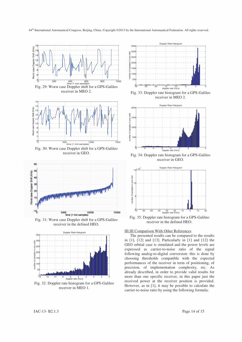
Doppler Shifts And Doppler Rates Because of the very high relative velocity between

the GNSS satellites and the orbiting receiver, the Doppler shift is much higher than for an Earth-based receiver. On figures 28, 29, 30, and 31, we present, for the four orbital cases considered and a full orbital period, the maximum or worst-case Doppler shift considering at any time all the visible satellites. As expected, the lower is the orbit; the higher is the maximum Doppler shift because the higher is the maximum relative velocity between receiver and transmitter. The highest value of approximately 55 kHz is in fact achieved at the beginning of the HEO when the receiver is in the lowest orbital point and accordingly it has the maximum velocity. Moreover, a considerable value of 20.5 kHz is achieved in MEO 1. In order to know how the Doppler shift changes in one full orbit for a given GNSS satellite, figures 32, 33, 34 and 35 illustrate the histogram of the Doppler rate values calculated for a receiver in the four considered orbits and the GPS and Galileo satellites.

Fig. 28: Worst case Doppler shift for a GPS-Galileo

receiver in MEO 1.

0 50 100 150 200 250 300 3500.65

0.7

0.75

0.8

0.85

0.9

time samples

GD

OP

GDOP For GPS-Galileo Receiver In MEO At 10000 Km

0 200 400 600 800 10001

1.5

2

2.5

3

Time (samples)

GD

OP

GDOP For A GPS-Galileo Receiver In MEO At 25000 Km

0 500 1000 15003

3.5

4

4.5

5

5.5


GD

OP

GDOP For A GPS-Galileo Receiver In GEO

0 50 100 150 200 250 300 3508

10

12

14

16

18

20

22

time (1 min samples)

Wors

t C

ase D

opple

r S

hift (K

Hz)

Worst Case Doppler Shift


IAC-13- B2.1.3 Page 14 of 15


receiver in MEO 2.


receiver in GEO.


receiver in the defined HEO.

Fig. 32: Doppler rate histogram for a GPS-Galileo

receiver in MEO 1.


receiver in MEO 2.


receiver in GEO.


receiver in the defined HEO. III.III Comparison With Other References

The presented results can be compared to the results in [1], [12] and [13]. Particularly in [1] and [12] the GEO orbital case is simulated and the power levels are expressed as carrier-to-noise ratio of the signal following analog-to-digital conversion: this is done by choosing thresholds compatible with the expected performances of the receiver in term of positioning, of precision, of implementation complexity, etc. As already described, in order to provide valid results for more than one specific receiver, in this paper just the received power at the receiver position is provided. However, as in [1], it may be possible to calculate the carrier-to-noise ratio by using the following formula:

0 200 400 600 800 10004

6

8

10

12

14

16

18


Wors

t case D

opple

r S

hift (K

Hz)

0 500 1000 15006

7

8

9

10

11

12

13

14

15


Wors

t case D

opple

r Shift (K

Hz)

-14 -12 -10 -8 -6 -4 -2 0 2 40

50

100

150

200

250

300

350Doppler Rate Histogram

doppler rate (Hz/s)

num

ber

of

sam

ple

s in o

ne o

rbit

-30 -25 -20 -15 -10 -5 0 50

500

1000

1500

2000

2500

3000


doppler rate (Hz/s)

num

ber

of sam

ple

s in o

ne o

rbit

-6 -5 -4 -3 -2 -1 0 1 20

500

1000

1500


doppler rate (Hz/s)

num

ber

of sam

ple

s in o

ne o

rbit

-70 -60 -50 -40 -30 -20 -10 0 10 200

5

10

15x 10

4 Doppler Rate Histogram

doppler rate (Hz/s)

num

ber

of sam

ple

s in o

ne o

rbit


IAC-13- B2.1.3 Page 15 of 15

3 4�� 5� ��6789:9; � �/< � �. [2] Where:

3 4�� is the carrier-to-noise ratio

�� is the received power in dBW

7 is the Boltzmann’s constant,

89:9 is the effective system noise temperature in Kelvin

�/< is the noise figure of the receiver front-end in dB

�. is the implementation and A/D conversion losses in dB.

If as in [1] we assume ��/< � �=>? dB, �. � � dB and 89:9 � 5@��A and considering the values in table 2 to acquire and/or track at least four GPS satellites simultaneously, the carrier-to-noise ratio in the GEO orbital case will have a minimum of 25.4 dB-Hz and a peak of 40.3 dB-Hz. The minimum of 25.4 dB-Hz is therefore not too far from the reported value of 29 dB-Hz in [1] and [12]. One reason for this difference is because in [1] the received power BC is calculated�as a sum of constant contributions, by assuming a constant gain for the transmitting antenna, while in our study, as already described, the gain is function of the antenna elevation and azimuth. IV. CONCLUSIONS The simulation performed using the multi-GNSS constellation simulator “Spirent GSS8000" have shown four examples of GNSS use for space applications from MEO to HEO with apogee close to the Lunar altitude. The simulations results indicate that in order to acquire and track at least four satellites simultaneously, a GPS receiver must be designed in such a way to acquire and track a -134.2 dBm signal in MEO 1, a -141.2 dBm signal in MEO 2, a -144.9 dBm signal in GEO and a -162.7 dBm in the defined HEO. Similarly, a GPS-Galileo-combined receiver will need to acquire and track a -120.8 dBm signal in MEO 1, a -131.6 dBm signal in MEO 2, a -134.6 dBm signal in GEO and a -153.8 dBm in the defined HEO. Furthermore the receiver should be able to acquire/track signals affected by a Doppler shift of approximately 21 kHz in MEO 1, 17 kHz in MEO 2, 15 kHz in GEO and 55 kHz in the low altitude part of the defined HEO. As expected, the MEO 1 is the orbit that shows the highest Doppler rate absolute value of almost 14 Hz/s for a not negligible number of orbit samples. The atmosphere delay

simulations have shown a mean delay of about 22 meters for MEO 2, GEO and the defined HEO and a mean of about 24 meters for MEO 1. The GDOP analysis instead, has proved the relative degradation of geometry as the altitude increases, as expected. Finally, simulation results have shown the significant GNSS performance improvements achievable by using a multi constellation receiver. V. REFERENCES [1] Michael S. Braasch and Maarten Uijt de Haag.

GNSS For LEO, GEO, HEO and Beyond. Advances in the astronautical sciences, pages 165-194, 2006.

[2] James J. Miller, Enabling a Fully Interoperable

GNSS Space Service Volume. 6thInternational Committee on GNSS (ICG), Tokyo, Japan, September 5-9, 2011.

[3] Elliot D. Kaplan, Christopher J. Hegarty. Understanding GPS: Principles and Applications, Artech House, 2006.

[4] Comprehensive Test Capabilities For Space-Based

GNSS Applications, http://www.spirent.com/Positioning-and-Navigation/GPS_GNSS_Test_Solutions_for_SpaceBased_Applications, 2nd September 2013

[5] Spirent, Simgen Software User Manual, issue 4-02 SR02, 13th December 2012.

[6] NATO Standard Agreement STANAG 4294 Issue 1.

[7] J. Sanz Subirana, J.M. Juan Zornoza and M. Hernández-Pajares, NeQuick Ionospheric Model,

http://www.navipedia.net/index.php/NeQuick_Ionospheric_Model, Technical University of Catalonia, Spain, 2nd September 2013.

[8] ICD-GPS-200F Navstar GPS Space Segment/User

Segment Interfaces (21 September 2011). [9] Galileo_SISICD V13.2 June 2009. [10] Francis M. Czopek, Scott Shollenberger,

Description and Performance of the GPS Block I

and II L-Band Antenna and Link Budjet, (ION GPS 1993).

[11] Mojtaba Bahrami, GNSS Doppler Positioning, University College London, 2008.

[12] Arnaud Dion, Vincent Calmettes, Michel Bousquet, Emmanuel Boutillon, Performances of a GNSS

receiver for space-based applications, Toulouse Space Show 2010.

[13] GiovanniB.Palmerini, MarcoSabatini, GiorgioPerrotta, En route to the Moon using GNSS

signals, Acta Astronautica 64 (2009) 467–483. [14] Norsuzila Ya’acob, Mardina Abdullah, Mahamod

Ismail, GPS Total Electron Content (TEC)

Prediction at Ionosphere Layer over the Equatorial

Region.

Documents

Mr. Vincenzo Capuano Dr. Cyril Botteron Prof. Pierre-André ... · Mr. Vincenzo Capuano École Polytechnique Fédérale de Lausanne (ESPLAB), Switzerland, [email protected]