MPUC E-999/CI-14-643 OFFICE OF ADMINISTRATIVE HEARINGS … · OAH 80-2500-31888 . MPUC E-999/CI-14-643 . STATE OF MINNESOTA . OFFICE OF ADMINISTRATIVE HEARINGS . FOR THE PUBLIC UTILITIES

OAH 80-2500-31888 MPUC E-999/CI-14-643

STATE OF MINNESOTA OFFICE OF ADMINISTRATIVE HEARINGS

FOR THE PUBLIC UTILITIES COMMISSION

In the Matter of the Further Investigation into Environmental and Socioeconomic Costs Under Minnesota Statutes Section 216B.2422, Subdivision 3

TABLE OF CONTENTS

I. Procedural History ................................................................................................. 2

II. Organization of this Report .................................................................................... 8

FINDINGS OF FACT ....................................................................................................... 9

I. Background ........................................................................................................... 9

II. Climate Change ................................................................................................... 10

A. Peabody Criticism of Climate Change: Natural Variability of the Earth’s Climate ................................................................................................................... 11

B. Peabody Criticism of Climate Change: Global Temperature Changes ........... 12

C. Peabody Criticism of Climate Change: Extreme Weather Events ................... 13

D. Peabody Criticism of Climate Change: Benefits from Increased CO2 Concentrations and Warmer Temperatures ........................................................... 14

E. Response to Peabody Criticism of Climate Change: Natural Variability of the Earth’s Climate ....................................................................................................... 15

F. Response to Peabody Criticism of Climate Change: Global Temperature Changes ................................................................................................................. 16

G. Response to Peabody Criticism of Climate Change: Extreme Weather Events .................................................................................................................... 19

H. Response to Peabody Criticism of Climate Change: Benefits from Increased CO2 Concentrations and Warmer Temperatures .................................................... 19

[70412/1] ii

I. Additional Findings Regarding Climate Change .............................................. 21

J. Administrative Law Judge’s Conclusions Regarding Climate Change ............. 23

III. The Federal Social Cost of Carbon ..................................................................... 23

A. Federal Social Cost of Carbon Background ..................................................... 23

B. The IWG FSCC Development Process: Overview ........................................... 25

C. Modeling Relationships: the Global Economy, Emissions, Warming and Damages ................................................................................................................ 26

D. The Three IAMs Chosen by the IWG ............................................................... 29

1. The DICE Model ........................................................................................ 29

2. The PAGE Model ....................................................................................... 31

3. The FUND Model ....................................................................................... 31

E. Implementation of the IAMs ............................................................................. 33

1. The IWG’s Modifications of the IAMs: Standardization ............................. 33

2. Socioeconomic Scenarios ......................................................................... 34

3. Equilibrium Climate Sensitivity ................................................................... 35

4. The Discount Rate for Converting Future Damages into Present Values .. 37

5. The Damage Functions ............................................................................. 38

6. Running the IAMs to Produce the FSCC ................................................... 40

F. IWG’s Acknowledgement of Limitations ........................................................... 44

IV. Criticisms of the Federal Social Cost of Carbon .................................................. 44

A. The IWG’s Use of the IAMs as Damage Cost Models ..................................... 45

1. Criticisms ................................................................................................... 45

2. Responses ................................................................................................. 49

B. Discount Rates ................................................................................................ 53

1. Criticisms ................................................................................................... 53

2. Responses ................................................................................................. 56

a. Xcel’s Public Policy Approach ................................................................... 56 b. The Agencies’ Consumption Rate of Discount Response ......................... 57

[70412/1] iii

c. The Agencies’ Response to the Ramsey Rule .......................................... 58 d. The Agencies’ Response to the Rate of Time Preference ......................... 60

e. The Agencies’ Response to Recommendations Regarding the Market Rate of Interest ................................................................................................. 61 f. The Agencies’ and CEOs’ Responses to the Seven Percent Discount Rate ................................................................................................................. 62

g. The Agencies’ and CEOs’ Discount Rate Conclusions .............................. 63

C. 95th Percentile Value at 3 Percent Discount Rate ............................................ 64

1. Criticisms ................................................................................................... 64

2. Responses ................................................................................................. 64

D. Equilibrium Climate Sensitivity ......................................................................... 65

1. Criticisms ................................................................................................... 65

2. Responses ................................................................................................. 67

E. Marginal Ton: last unit of CO2 emitted.............................................................. 70

1. Criticisms ................................................................................................... 70

2. Responses ................................................................................................. 72

F. Modeling Time Horizon: Estimates of damages after 2100 ............................. 73

1. Criticisms ................................................................................................... 73

2. Responses ................................................................................................. 74

G. Geographic Scope ........................................................................................... 76

1. Criticisms ................................................................................................... 76

2. Responses ................................................................................................. 77

H. Leakage ........................................................................................................... 79

1. Criticisms ................................................................................................... 79

2. Responses ................................................................................................. 82

[70412/1] iv

I. Uncertainty ....................................................................................................... 84

1. Criticisms ................................................................................................... 84

2. Responses ................................................................................................. 86

J. Adaptation and Mitigation ................................................................................ 87

1. Criticisms ................................................................................................... 87

2. Responses ................................................................................................. 89

K. Use of FSCC Outside of Regulatory Setting .................................................... 89

1. Criticisms ................................................................................................... 89

2. Responses ................................................................................................. 91

L. Whether the IWG Used a Scientific Process .................................................... 92

1. Criticisms ................................................................................................... 92

2. Responses ................................................................................................. 93

V. Parties’ Conclusions and Recommendations ...................................................... 96

A. Utilities and MLIG............................................................................................. 96

B. MLIG ................................................................................................................ 98

C. Peabody ........................................................................................................... 99

VI. Xcel Energy Proposal ........................................................................................ 101

VII. Criticisms of Xcel Proposal ................................................................................ 109

A. The median versus the mean ........................................................................ 109

B. The range of values ....................................................................................... 110

C. Averaging the discount rates ......................................................................... 111

D. Exclusion of 95th Percentile of FSCC Distribution .......................................... 112

E. Xcel’s Criteria for Reviewing the FSCC ......................................................... 112

F. Use of the Underlying FSCC Data ................................................................. 113

G. Xcel’s Responses to Criticisms of Its Proposal .............................................. 113

[70412/1] v

CONCLUSIONS .......................................................................................................... 114

I. Use of IAMS as Damage Cost Models .............................................................. 115

II. IWG’s Choice and Application of Discount Rates .............................................. 116

III. 95th Percentile Value at 3 Percent Discount Rate .............................................. 117

IV. Equilibrium Climate Sensitivity .......................................................................... 118

V. Marginal Ton ..................................................................................................... 118

VI. Modeling Time Horizon ..................................................................................... 119

VII. Geographic Scope ............................................................................................. 120

VIII. Leakage ............................................................................................................ 121

IX. Uncertainty ........................................................................................................ 121

X. Adaptation and Mitigation .................................................................................. 121

XI. Use of FSCC Outside of Federal Regulatory Setting ........................................ 121

XII. Scientific Process .............................................................................................. 122

XIII. Xcel Proposal .................................................................................................... 122

XIV. Reasonable and the Best Available Measure of CO2 ........................................ 123

RECOMMENDATIONS ............................................................................................... 123

NOTICE ....................................................................................................................... 124

MEMORANDUM ......................................................................................................... 125

I. Guiding Criteria ................................................................................................. 125

II. Adopting Conservative Values .......................................................................... 125

III. DHE and CEBC Testimony ............................................................................... 127

IV. DHE Testimony ................................................................................................. 127

V. CEBC Testimony ............................................................................................... 129

VI. Modeling Time Horizon ..................................................................................... 129

VII. Xcel’s Proposal .................................................................................................. 130

[70412/1] vi

VIII. Use of the FSCC to Fulfill the Requirements of Minn. Stat. § 216B.2422 ......... 130

ATTACHMENT A: LIST OF PARTIES AND THEIR EXPERT WITNESSES ............... 132

ATTACHMENT B: SUMMARY OF PUBLIC COMMENT ............................................. 137

I. Public Hearing Comments ................................................................................. 138

II. Written Public Comments .................................................................................. 140

OAH 80-2500-31888 MPUC E-999/CI-14-643



In the Matter of the Further Investigation into Environmental and Socioeconomic Costs Under Minnesota Statutes Section 216B.2422, Subdivision 3

FINDINGS OF FACT, CONCLUSIONS, AND

RECOMMENDATIONS: CARBON DIOXIDE VALUES

This matter is pending before Administrative Law Judge LauraSue Schlatter pursuant to a Notice and Order for Hearing filed by the Public Utilities Commission (Commission) on October 15, 2014.1

On September 24 – 30, 2015, the evidentiary hearing for the carbon dioxide (CO2) portion of this matter took place at the Commission’s office in Saint Paul, Minnesota. Appearances:2 Kevin Reuther, Leigh Currie, and Hudson Kingston, attorneys with the Minnesota Center for Environmental Advocacy, appeared on behalf of the Minnesota Center for Environmental Advocacy, Fresh Energy, and Sierra Club, collectively the Clean Energy Organizations (CEOs). Tristan L. Duncan, attorney with Shook, Hardy & Bacon L.L.P., and Jonathan Massey, Attorney at Law, appeared on behalf of Peabody Energy Corporation (Peabody). Linda Jensen, Assistant Attorney General, appeared on behalf of the Minnesota Department of Commerce, Division of Energy Resources (Department), and the Minnesota Pollution Control Agency (MPCA) (collectively the Agencies). Eric F. Swanson, attorney with Winthrop & Weinstine P.A., appeared on behalf of the Lignite Energy Council (Lignite). B. Andrew Brown, attorney with Dorsey & Whitney L.L.P., appeared on behalf of Great River Energy (GRE), Minnesota Power Company (MP), and Otter Tail Power Company (OTP) (collectively the Utilities). David Moeller, attorney with Minnesota Power Company, appeared on behalf of Minnesota Power Company (MP). 1 NOTICE AND ORDER FOR HEARING (Oct. 15, 2014) (eDocket No. 201410-103872-02). 2 A list of the parties and their expert witnesses is attached as Appendix A.

[70412/1] 2

James R. Denniston, Assistant General Counsel, appeared on behalf of Northern States Power Company, d/b/a Xcel Energy (Xcel). Marc Al and Andrew P. Moratzka, attorneys with Stoel Rives L.L.P., appeared on behalf of Minnesota Large Industrial Group (MLIG). Benjamin L. Gerber, Attorney at Law, appeared on behalf of the Minnesota Chamber of Commerce (MCC). Kevin P. Lee, Attorney at Law, appeared on behalf of Doctors for a Healthy Environment (DHE). Bradley Klein and Jessica Dexter, attorneys with the Environmental Law & Policy Center, appeared on behalf of the Clean Energy Business Coalition (CEBC).

Tricia DeBleeckere, Energy Analyst, and Sean Stalpes, Energy Analyst, were present at the hearing on behalf of the staff of the Commission. I. Procedural History

1. In 1993, the Minnesota Legislature enacted Minnesota Statute section 216B.2422, subdivision 3, which requires the Commission to “quantify and establish a range of environmental costs associated with each method of electricity generation.” In addition, the statute requires utilities to use the costs “when evaluating and selecting resource options in all proceedings before the [C]ommission, including resource planning and certificate of need proceedings.”3

2. In 1994, the Commission established interim cost values, and in 1997, the Commission established final values, after a contested case proceeding (first Externalities case).4 The Commission’s 1997 decision establishing final values was affirmed by the Minnesota Court of Appeals.5

3. On October 9, 2013, several environmental advocacy organizations filed a

motion requesting that the Commission update the cost values for carbon dioxide (CO2) and nitrogen oxide (NOx) emissions, establish a cost value for particulate matter less than 2.5 microns in diameter (PM2.5), and re-establish a value for sulfur dioxide (SO2). In the

3 1993 Minn. Laws ch. 356, § 3 at 2523. 4 In the Matter of the Quantification of Envtl Costs Pursuant to Laws of Minn. 1993, Chap. 356, Sec. 3, PUC Docket No. E-999/CI-93-583, ORDER ESTABLISHING ENVIRONMENTAL COST VALUES at 1, 33 (Jan. 3, 1997) (see also eDocket No. 20148-102561-01) (93-583 PUC ORDER 1); In the Matter of the Quantification of Envtl Costs Pursuant to Laws of Minn. 1993, Chap. 356, Sec. 3, PUC Docket No. E-999/CI-93-583, ORDER AFFIRMING IN PART AND MODIFYING IN PART ORDER ESTABLISHING ENVIRONMENTAL COST VALUES at 8 (July 2, 1997) (see also eDocket No. 201410-103872-02) (93-583 PUC ORDER 2). 5 In re Quantification of Envtl Costs, 578 N.W.2d 794 (Minn. Ct. App. 1998), review denied (Minn. Aug. 18, 1998).

[70412/1] 3

motion, the environmental organizations recommended that the Commission adopt the federal government’s Social Cost of Carbon as the cost value for CO2.6

4. On February 10, 2014, the Commission issued an order reopening its

investigation into “the appropriate range of externality [cost] values for PM2.5, SO2, NOx, and CO2.”7 The Commission ordered the Agencies to convene a stakeholder group to provide recommendations on the scope of the reopened Externalities investigation.8

5. On June 10, 2014, the Agencies filed a report stating that there was little

stakeholder consensus. The Agencies recommended that the Commission adopt the federal Social Cost of Carbon midpoint values for CO2,9 and also made recommendations about the scope and process of the Commission investigation and retention of an expert.10

6. On October 15, 2014, the Commission issued the Notice and Order for

Hearing for this matter, which set the scope of the reopened Externalities investigation as follows:

The Commission will investigate the appropriate cost values for PM2.5, SO2, NOx, and CO2. The Commission will not further investigate at this time the environmental costs of other greenhouse gasses such as methane (CH4), nitrous oxide (N2O), hydrofluorocarbons (HFCs), perfluorocarbons (PFCs), and sulfur hexafluoride (SF6). Because CO2 represents 99% of greenhouse gas emissions, an accurate environmental cost value for CO2 will account for almost all greenhouse gas costs. This will result in a more manageable proceeding and allow the parties to focus their resources.

It would be premature at this stage to adopt the federal SCC values for CO2 as the Agencies recommend. The Commission still believes that a contested case proceeding is necessary to fully consider the Agencies’ proposed CO2 cost values. The Commission will therefore not act at this time on the Agencies’ proposal to adopt the federal SCC values immediately. But, in light of the record so far, the

6 In the Matter of the Investigation into Environmental and Socioeconomic Costs Under Minn. Stat. § 216B.2422, Subd. 3, PUC Docket No. E-999/CI-00-1636, MEMORANDUM IN SUPPORT OF CLEAN ENERGY ORGANIZATIONS’ MOTION TO UPDATE EXTERNALITY VALUES FOR USE IN RESOURCE DECISIONS at 1-2, 18-19 (Oct. 9, 2013). 7 In the Matter of the Investigation into Environmental and Socioeconomic Costs Under Minn. Stat. § 216B.2422, Subd. 3, PUC Docket No. E-999/CI-00-1636, ORDER REOPENING INVESTIGATION AND CONVENING STAKEHOLDER GROUP TO PROVIDE RECOMMENDATIONS FOR CONTESTED CASE PROCEEDING at 3 (Feb. 10, 2014). 8 Id. 9 In the Matter of the Investigation into Environmental and Socioeconomic Costs Under Minn. Stat. § 216B.2422, Subd. 3, PUC Docket No. E-999/CI-00-1636, COMMENTS BY DOC-DER AND MPCA at 9-10 (June 10, 2014). 10 Id. at 16-17.

[70412/1] 4

Commission will ask the Administrative Law Judge to determine whether the Federal Social Cost of Carbon is reasonable and the best available measure to determine the environmental cost of CO2 and, if not, what measure is better supported by the evidence.

The Commission will require parties in the contested case proceeding to evaluate the costs using a damage cost approach, as opposed to (for example), market-based or cost-of-control values. When last faced with the question of the preferred approach to estimate environmental cost values, the Commission stated that, as between estimates based on damage or based on cost-of-control, the damage-cost approach is superior because it appropriately focuses on actual damages from uncontrolled emissions.

Nothing in this proceeding justifies reaching a different conclusion now. Where a damage cost can be reasonably estimated, it represents a superior method of valuing an emission’s environmental cost. The Commission is persuaded that a damage-cost approach can be used for the emissions under investigation, and will therefore require it.11

7. The Commission referred the matter to the Office of Administrative Hearings

to address the following issues:

a. Whether the Federal Social Cost of Carbon is reasonable and the best available measure to determine the environmental cost of CO2 under Minn. Stat. § 216B.2422 and, if not, what measure is better supported by the evidence; and

b. The appropriate values for PM2.5, SO2, and NOx [the criteria pollutants] under Minn. Stat. § 216B.2422, subd. 3.12

8. Following a prehearing conference on November 14, 2014, the Administrative Law Judge issued an order granting intervention to OTP, MP, Lignite, Xcel, MLIG, GRE, and the MCC as full parties in this matter.13 In addition, the Administrative Law Judge ordered the proceedings to be bifurcated. Testimony regarding CO2 and the criteria pollutants would be prefiled according to separate schedules, with separate evidentiary hearings scheduled.14

11 NOTICE AND ORDER FOR HEARING at 4-5 (Oct. 15, 2014) (eDocket No. 201410-103872-02). 12 Id. 13 FIRST PREHEARING ORDER at 3 (Dec. 9, 2014) (eDocket No. 201412-105272-01). In addition to the Department, the CEOs and Peabody were the only parties named in the Commission’s Notice and Order for Hearing issued on October 15, 2014. 14 FIRST PREHEARING ORDER at 4 (Dec. 9, 2014) (eDocket No. 201412-105272-01).

[70412/1] 5

9. On March 19, 2015, the Administrative Law Judge granted intervention to the MPCA as a full party in this matter.15

10. On March 27, 2015, the Administrative Law Judge issued an order

addressing the evidentiary burdens of proof for this matter. After considering the parties’ arguments, the Administrative Law Judge set forth the following parameters for the evidentiary burdens of proof:

a. A party or parties proposing that the Commission adopt a new

environmental cost value for CO2, including the Federal Social Cost of Carbon, bears the burden of showing, by a preponderance of the evidence, that the value being proposed is reasonable and the best available measure of the environmental cost of CO2.

b. A party or parties proposing that the Commission adopt a new environmental cost value for one or more of the criteria pollutants – SO2, NOx, and/or PM2.5 – bears the burden of showing, by a preponderance of the evidence, that the cost value being proposed is reasonable, practicable, and the best available measure of the criteria pollutant’s cost.

c. A party or parties proposing that the Commission retain any

environmental cost value as currently assigned by the Commission bears the burden of showing, by a preponderance of the evidence, that the current value is reasonable and the best available measure to determine the applicable environmental cost.

d. An environmental cost value currently being applied by the

Commission is presumed to be practicable, as required by Minn. Stat. § 216B.2422, subd. 3. A party challenging an existing cost value on the grounds that it is not practicable bears the burden of demonstrating impracticability by a preponderance of the evidence.

e. A party or parties, opposing a proposed environmental cost value

must demonstrate, at a minimum, that the evidence offered in support of the proposed values is insufficient to amount to a preponderance of the evidence. This requirement does not apply to a party challenging an existing cost value based on its alleged impracticability, as described in paragraph 4, above.

15 ORDER GRANTING INTERVENTION TO MINNESOTA POLLUTION CONTROL AGENCY (Mar. 20, 2015) (eDocket No. 20153-108414-01).

[70412/1] 6

f. Any proponent of an environmental cost value, including existing environmental cost values, shall file direct testimony in support of its proposal according to the schedule set forth in the Second Prehearing Order in this matter.

g. A party advocating for retention of an existing cost value may not

refer by reference to evidence or testimony from the Commission’s CI-93-583 docket or related dockets, but must introduce any evidence on which it intends to rely in this docket, whether the evidence is drawn from an older docket or is new evidence.

h. A party may propose an environmental cost value not proposed

in direct testimony in the party’s rebuttal testimony only if the new cost value is offered in response to a cost value proposed in direct testimony.16

11. On April 16, 2015, the Administrative Law Judge issued an order concluding

that testimony regarding the efficacy of renewable energy or renewable energy policy was presumed to be irrelevant and would be excluded from this matter unless its relevance was specifically demonstrated.17 The Administrative Law Judge also granted intervention to DHE, the CBEC, and Interstate Power and Light Company as full parties in this matter.18

12. On May 27, 2015, the Commission issued an order requiring one public

hearing to be held for this matter.19 The Commission’s order also required that members of the public be allowed to submit written comments regarding this matter via mail or the Commission’s SpeakUp website.20 The Commission’s plan for providing the public notice of the public hearing and written comment period included publishing notice in the Environmental Quality Board Monitor and the MPCA’s electronic newsletter, posting notice on state agency websites, issuing a press release, and directly providing the notice to all county administrators.21

13. On June 2, 2015, the Commission issued a notice for the public hearing and

of the written comment period.22

16 ORDER REGARDING BURDENS OF PROOF at 2-3 (Mar. 27, 2015) (eDocket 20153-108636-01). 17 THIRD PREHEARING ORDER at 2 (Apr. 16, 2015) (eDocket No. 20154-109385-01). 18 ORDER GRANTING INTERVENTION TO DOCTORS FOR A HEALTHY ENVIRONMENT, CLEAN ENERGY BUSINESS COALITION, AND INTERSTATE POWER AND LIGHT COMPANY (Apr. 16, 2015) (eDocket No. 20154-109386-01). Interstate Power and Light Company later withdrew from the proceeding. See Interstate Power and Light Company Letter Withdrawing (Aug. 13, 2015) (eDocket No. 20158-113202-01). 19 ORDER REQUIRING PUBLIC HEARING at 2 (May 27, 2015) (eDocket 20155-110744-01). 20 Public Hearing and Comment Period Notice Plan (May 29, 2015) (eDocket 20155-110942-01). 21 Id. 22 Notice of Public Hearing and Comment Period (June 2, 2015) (eDocket No. 20156-111067-01).

[70412/1] 7

14. On June 1, 2015, the parties filed direct testimony in the CO2 portion of this matter.

15. On August 5, 2015, parties filed direct testimony in the criteria pollutants

portion of this matter. 16. On August 12, 2015, parties filed rebuttal testimony in the CO2 portion of

this matter. 17. On August 26, 2015, the public hearing was held at the Commission’s office

in Saint Paul.23 18. On September 10, 2015, parties filed surrebuttal testimony in the CO2

portion of this matter. 19. On September 15, 2015, the Administrative Law Judge filed two orders

deciding several different motions to strike and exclude testimony. The Administrative Law Judge denied motions to strike all or portions of the testimony of Dr. Michael Hanemann, Dr. Stephen Polasky, Mr. Nicholas Martin, Mr. Shawn Rumery, and Mr. Christopher Kunkle.24 The Administrative Law Judge granted a motion to strike a portion of the testimony of Dr. William Happer.25

20. On September 21, 2015, the Administrative Law Judge issued an order

deciding additional motions to strike and exclude testimony. The Administrative Law Judge denied motions to strike portions of the testimony of Dr. John Abraham, Dr. Andrew Dessler, and Dr. Kevin Gurney.26 The Administrative Law Judge granted a motion to strike a portion of the testimony of Dr. Peter Reich.27

21. On September 24 – 30, 2015, the evidentiary hearing for the CO2 portion of

this matter took place at the Commission’s office in Saint Paul. 22. On October 30, 2015, the parties filed rebuttal testimony in the criteria

pollutants (PM2.5, SO2, NOx) portion of this matter.

23 A summary of the public hearing testimony, exhibits, and written public comments is attached as Appendix B. 24 ORDER ON MOTIONS BY MINNESOTA LARGE INDUSTRIAL GROUP AND PEABODY ENERGY CORPORATION TO EXCLUDE AND STRIKE TESTIMONY at 2 (Sept. 15, 2015) (eDocket No. 20159-113992-01); ORDER ON MOTIONS BY PEABODY ENERGY CORPORATION, MINNESOTA DEPARTMENT OF COMMERCE, AND POLLUTION CONTROL AGENCY TO EXCLUDE AND STRIKE TESTIMONY at 2 (Sept. 15, 2015) (eDocket No. 20159-113998-01). 25 ORDER ON MOTIONS BY PEABODY ENERGY CORPORATION, MINNESOTA DEPARTMENT OF COMMERCE, AND POLLUTION CONTROL AGENCY TO EXCLUDE AND STRIKE TESTIMONY at 2 (Sept. 15, 2015) (eDocket No. 20159-113998-01). The Administrative Law Judge excluded a single photograph of a weather thermometer hanging on a house above a charcoal grill, finding the photograph’s probative value was outweighed by its prejudicial effect. 26 ORDER ON MOTIONS BY MINNESOTA LARGE INDUSTRIAL GROUP AND PEABODY ENERGY CORPORATION TO EXCLUDE AND STRIKE TESTIMONY at 2-3 (Sept. 21, 2015) (eDocket No. 20159-114135-01). 27 Id. A single sentence of Dr. Reich’s surrebuttal testimony was excluded as irrelevant because it addressed the impact climate change might have on the needs of wildlife in particular types of habitat.

[70412/1] 8

23. On November 12, 2015, the issues matrix for the CO2 portion of this matter

was filed.28 24. On November 24, 2015, parties filed initial briefs in the CO2 portion of this

matter. On the same date, the Administrative Law Judge issued an order denying motions to strike and exclude the testimony of Mr. Richard Rosvold and Dr. Roger McClellan in the criteria pollutants portion of this matter.29

25. On December 4, 2015, the parties filed surrebuttal testimony in the criteria

pollutants portion of this matter. 26. On December 15, 2015, parties filed reply briefs and proposed findings in

the CO2 portion of this matter. 27. On January 12-14, 2016, the evidentiary hearing for the criteria pollutants

portion of this matter took place at the Commission’s office in Saint Paul. 28. On March 1, 2016, the issues matrix for the criteria pollutants portion of this

matter was filed.30 29. On March 15, 2016, the parties filed initial briefs in the criteria pollutants

portion of this matter. 30. On April 15, 2016, the parties filed reply briefs and proposed findings in the

criteria pollutants portion of this matter. 31. The Administrative Law Judge is scheduled to issue her Report in the

criteria pollutants portion of this matter on June 15, 2016.

II. Organization of this Report 32. In order to best accommodate all of the parties and their arguments in this

proceeding, this Report is organized as described in the following paragraphs. 33. Section I provides introductory substantive background regarding the

proceeding and the Report. 34. Section II sets forth Peabody’s arguments regarding the existence, cause,

and benefits of climate change, followed by the various parties’ responses to Peabody’s arguments and a section of Additional Findings of Fact. This section includes

28 C02 Issues Matrix (Nov. 12, 2015) (eDocket No. 201511-115671-01). 29 ORDER ON MOTIONS BY DEPARTMENT OF COMMERCE, POLLUTION CONTROL AGENCY AND CLEAN ENERGY ORGANIZATIONS TO EXCLUDE AND STRIKE TESTIMONY at 2 (Nov. 24, 2015) (eDocket No. 201511-115904-01). 30 Criteria Pollutants Issues Matrix (Mar. 1, 2016) (eDocket No. 20163-118846-01).

[70412/1] 9

Conclusions of Law by the Administrative Law Judge regarding Peabody’s climate change arguments.

35. Section III provides a detailed description of the background, development,

modeling, and implementation of the process used to calculate the federal social cost of carbon (FSCC). Section IV includes the various parties’ criticisms of specific aspects of the FSCC and processes related to its development. The responses to each set of criticisms follow immediately after the recitation of those criticisms. Section V presents the conclusions and recommendations of the Utilities, MLIG and Peabody regarding methodologies and costs for the social cost of carbon (SCC).

36. Section VI provides a description of Xcel’s proposal for calculating the SCC.

Section VII presents other parties’ criticisms, and Xcel’s responses, to its SCC proposal.

37. The Administrative Law Judge’s Conclusions of Law and Recommendations are followed by a Memorandum. Appendix A provides a brief description of each witness who provided testimony in this proceeding, by party. Appendix B summarizes public comments.

FINDINGS OF FACT

I. Background 1. The task of the Administrative Law Judge in the CO2 portion of this matter

is to review and synthesize information related to the complex issues of climate change science, economics, and public policy in order to recommend an updated externality or cost value for carbon dioxide emissions produced by electricity generation in Minnesota.

2. When an economic activity imposes a cost or benefit on an unrelated third party, the cost or benefit is known as an economic external cost or “externality.”31 Externalities can be viewed as positive or negative depending on their impact.32 This portion of this proceeding focuses on the externalities created as a result of CO2 emissions produced while generating electricity.

3. Environmental economics, as used in this proceeding, focuses on the costs of externalities from electricity generation in order to develop and implement public policies, such as government regulations and tax remedies aimed at reducing environmental damages.33 The results of this proceeding will affect how utilities in Minnesota select, allocate, and build resources for the future.

4. When it set final cost values pursuant to Minn. Stat. § 216B.2422, subd. 3 in the January 1997 Order in the first Externalities case, the Commission established several principles to guide its quantification of those values. These principles, as applicable to CO2 cost values, included a) a preference that a damage-cost approach be 31 Ex. 800 at 7-8 (Hanemann Direct). 32 Id. 33 Ex. 800 at 10, 12-13 (Hanemann Direct).

[70412/1] 10

used; b) establishment of a range of values to appropriately take into consideration a level of uncertainty; and c) use of a global basis to establish damages for CO2 values.34

5. In its July 1997 Order in the first Externalities case, the Commission found “that CO2 is markedly different from the other pollutants for which it has established ranges of environmental costs.”35 Specifically, the Commission acknowledged that the uncertainties inherent in the assumptions necessary to provide a meaningful estimate of potential costs from CO2 emissions, as well as those uncertainties connected to discounting to present value “the significant damage costs assumed to occur many years into the future,” made quantifying externality cost values for CO2 complex.36 Despite the complexity of these uncertainties, the Commission concluded that it was “practicable to establish an environmental cost range for carbon dioxide.”37

6. The Commission’s concern in 1997 with the complexity of calculating the environmental cost value of CO2 arises from the nature of CO2 itself. Emissions of CO2 mix into the atmosphere when they are released. They travel around the Earth and remain in the atmosphere for hundreds of years. Thus, their impacts are felt around the globe for several hundred years.38

7. Because of the extended time period involved, it is not possible to develop a methodology to estimate the externality value for CO2 based solely on empirical evidence in the record. Many modeling assumptions about the future – such as population, income, gross domestic product (GDP), emissions, damage functions, equilibrium climate sensitivity (ECS), technological change, adaptation, and mitigation – rely on estimates about the future based on current experience and evidence.39 Thus, one of the primary questions in this proceeding is which of the approaches or combinations of approaches, proposed by the parties, best accounts for the future uncertainties.

II. Climate Change

8. Peabody asserted that significant climate change is not occurring or, to the extent climate change is occurring, it is not due to anthropogenic causes. Furthermore, Peabody insisted that any current warming and increased CO2 in the Earth’s atmosphere are beneficial. Based on its position on climate change, Peabody maintained that the

34 93-583 PUC ORDER 1 at 14-15. The Commission’s January 1997 Order in the 1997 Externalities docket required the CO2 cost values to be applied to facilities built within a 200-mile radius outside of Minnesota’s borders. The reasoning behind this decision was an attempt to be consistent with the Commission’s approach to the criteria pollutants. On reconsideration, in July 1997, the Commission declined to use its authority to apply the CO2 values to facilities beyond Minnesota’s border. 93-583 PUC ORDER 2 at 3-5. 35 93-583 PUC ORDER 2 at 4. 36 93-583 PUC ORDER 2 at 4. 37 Id. 38 Ex. 805 at 2 (Hanemann Opening Statement). 39 Ex. 600 at 5-6 (Martin Direct).

[70412/1] 11

externality value of CO2 would most accurately be set at or below zero.40 Peabody made several arguments in support of its position, which are discussed below.

A. Peabody Criticism of Climate Change: Natural Variability of the Earth’s Climate

9. Peabody argued that only half of the CO2 in the atmosphere is due to fossil fuel emissions. The remainder comes from natural processes.41 According to Peabody, the claim that all increases in atmospheric CO2 are from human causes is simply unfounded.42

10. Peabody maintained that CO2 emissions are not directly related to increasing concentrations of CO2 in the atmosphere. While CO2 emission rates roughly tripled between 1995 and 2002, Peabody pointed out that atmospheric CO2 concentrations “remained essentially unchanged during that time.”43 Thus, Peabody claimed “we are currently unable to relate atmospheric CO2 levels to temperature and still less to regional changes.”44

11. Peabody highlighted that climate change is not a new concept because the Earth’s temperature and the CO2 concentration in its atmosphere have varied quite significantly over time. According to Peabody, in earlier epochs, the Earth’s climate was significantly warmer and the atmosphere’s CO2 content was much higher.45 Peabody maintained there “is no indication that the Earth’s climate is ‘changing’ in any manner that is not otherwise naturally-occurring and consistent with climate change patterns that occurred long before the recent concern over anthropogenic emissions.”46 Peabody argued that the Earth has experienced much higher CO2 levels over most of the 550 million year history of multicellular living organisms without the higher CO2 levels inducing catastrophic climate change.47

40 Peabody Initial Brief (Br.) at 98 (Nov. 30, 2015). 41 Ex. 207 at 6 (Lindzen Direct). 42 Ex. 207 at 6 (Lindzen Direct); Ex. 213 at 29 (Lindzen Surrebuttal). 43 Ex. 207 at 6 (Lindzen Direct). 44 Id. 45 Ex. 207 at 2, 4, 11 (Lindzen Direct). The Earth has experienced the following warm periods: “the Medieval Warm period, the Holocene Optimum, several interglacial periods, and the Eocene (which was much warmer than the present).” Id. at 4; see also Ex. 228 at 2 (Bezdek Direct); Ex. 204 at 4 (Happer Rebuttal). 46 Ex. 207 at 2 (Lindzen Direct). 47 Ex. 204 at 4 (Happer Rebuttal Ex. 1).

[70412/1] 12

12. According to Peabody, climate change concerns focused on CO2 are not viable unless it is first proven that global warming caused by CO2 emissions is greater than warming caused by natural variability.48 Peabody argued that the Intergovernmental Panel on Climate Change (IPCC)49 simply assumed global warming caused by carbon dioxide emissions is greater than warming caused by natural variability, and therefore attributes the warming observed since the 1970s to anthropogenic causes.50 According to Peabody, the Earth’s climate record shows that global temperatures rose from 1895 to 1946 in a manner essentially indistinguishable from the warming that occurred between 1957 and 2008.51 Thus, Peabody took issue with the IPCC attributing all of the warming in the later period solely to human activity.52

13. To support its argument that the IPCC’s climate models greatly overestimate global warming, Peabody pointed to evidence that the United States was warmer during the Dust Bowl years of the 1930s than it has been since, and cited a study of United States data from 2005 to 2014 that suggests the climate is cooling.53

B. Peabody Criticism of Climate Change: Global Temperature Changes

14. According to Peabody, global atmospheric temperatures are measured by surface thermometers, weather balloons (radiosondes), and satellites.54 Peabody claimed all three methods of measuring atmospheric temperatures show no warming since 1998.55

15. Peabody stated that the IPCC’s climate models may generate warming that roughly fits the observational data of atmospheric temperatures from the 1970s into the 1990s, but Peabody determined that global average temperatures have failed to increase after 1998, as the models predicted. Peabody is not certain why the models failed.56 Peabody insisted that the climate models predicted much more atmospheric warming than has occurred, even as CO2 emissions have been at their highest levels.57

48 Ex. 209 at 3 (Lindzen Direct Ex. 2). 49 In 1988, the United Nations established the Intergovernmental Panel on Climate Change (IPCC), which is a scientific organization charged with producing reports supporting the United Nations Convention on Climate Change, an international treaty. The IPCC has published five climate science assessment reports in 1990, 1995, 2001, 2007, and 2014. The Commission and the Minnesota Court of Appeals recognize the IPCC as a source of expertise on climate change. See In the Matter of the Quantification of Envtl Costs Pursuant to Laws of Minn. 1993, Chap. 356, Sec. 3, PUC Docket No. E-999/CI-93-583, ORDER ESTABLISHING ENVIRONMENTAL COST VALUES at 24 (Jan. 3, 1997); In re Quantification of Envtl Costs, 578 N.W.2d 794, 800-01 (Minn. Ct. App. 1998), review denied (Minn. Aug. 18, 1998). 50 Ex. 207 at 2-3 (Lindzen Direct). 51 Id. at 4. 52 Id. 53 Ex. 233 at 9-10 (Bezdek Rebuttal Ex. 1). 54 Ex. 221 at 5-6 (Spencer Direct). 55 Id. 56 Ex. 200 at 4, 8 (Happer Direct); Ex. 207 at 3 (Lindzen Direct); Ex. 227 at 2-4 (Spencer Surrebuttal). 57 Ex. 207 at 3 (Lindzen Direct); Ex. 221 at 3-5 (Spencer Direct); Ex. 233 at 5 (Bezdek Rebuttal Ex. 1).

[70412/1] 13

16. In addition to overestimating atmospheric warming, Peabody alleged the IPCC’s climate models overestimated the amount of oceanic warming that has occurred.58

17. Peabody’s experts referred to the period after 1998 as the “hiatus” because, in contrast to the rising temperature trend observed beginning in the 1970s, the observational data after 1998 shows a flat or even declining trend in atmospheric temperatures.59

18. Peabody placed significant weight on the failure of the IPCC’s climate models to explain the hiatus in warming after 1998 except by the introduction of ad hoc mechanisms, such as aerosols.60 Peabody contended the IPCC’s climate models have no utility if they cannot reliably predict temperature change from CO2 emissions.61 The Integrated Assessment Models (IAMs) used to calculate the FSCC “make little sense today since they are based on climate models that clearly overestimate the warming from more CO2 by hundreds of per cents [sic].”62 Because the IPCC models failed to account for the hiatus in warming, Peabody argued the models are not reliable.63

C. Peabody Criticism of Climate Change: Extreme Weather Events

19. Peabody disputed that extreme weather events are becoming more severe or more frequent than in the past.64 Peabody noted that, even more certainly than climate change, increased populations and wealth have been found to be major causes of economic damages from extreme weather events.65 “Concerns arising from the potential impact of global warming on drought, flooding, storminess, sea ice, and similar issues are largely unproven. There is no evidence that these matters are increasing due to warming (or in most cases increasing at all).”66 Moreover, Peabody claimed there is no evidence of increased hurricanes, tornadoes, wildfires, or droughts despite increases in atmospheric CO2 levels.67

20. Furthermore, despite alarms over recent reports of rising sea levels, Peabody maintained that sea levels have been rising for a very long time.68 Peabody

58 Ex. 206 at 7 (Happer Surrebuttal). 59 Ex. 200 at 8 (Happer Direct); Ex. 221 at 6 (Spencer Direct). 60 Ex. 207 at 3 (Lindzen Direct); Ex. 202 at 6 (Happer Direct Ex. 2). “Aerosols” in the climate change context refer to “so-called sulfates,” which primarily “act as reflectors of visible light” and have a cooling effect because they reflect sunlight. Evidentiary Hearing Transcript Volume (Tr. Vol.) 2A at 37 (Lindzen). 61 Ex. 223 at 4 (Spencer Direct Ex. 2). 62 Ex. 200 at 4 (Happer Direct). 63 Id. at 9. 64 Ex. 228 at 32 (Bezdek Direct); Ex. 207 at 6-7 (Lindzen Direct); Ex. 200 at 9 (Happer Direct). 65 Ex. 213 at 38 (Lindzen Surrebuttal). 66 Ex. 207 at 6-7 (Lindzen Direct). 67 Ex. 228 at 32 (Bezdek Direct). 68 Ex. 207 at 7 (Lindzen Direct); Ex. 213 at 36-37 (Lindzen Surrebuttal).

[70412/1] 14

stated the rate of sea level rise was faster during the period from 1904 to 1953 than it has been since that time.69

21. Peabody highlighted that even the IPCC has retreated from claims concerning the connection between global warming and extreme weather. The IPCC’s most recent report, Climate Change 2013: The Physical Science Basis, Fifth Assessment Report (IPCC AR5),70 found the causal connection less certain than did the IPCC’s last version of the report published in 2007 (Fourth Assessment Report (IPCC AR4)).71

22. Peabody predicted that the actual impact of global warming will be to reduce extreme weather events.72 “The primary driving force for storm development is the temperature difference between the tropics and the poles, a difference that should be decreasing if there is global warming, which is supposed to be greater at the poles.”73

D. Peabody Criticism of Climate Change: Benefits from Increased CO2 Concentrations and Warmer Temperatures

23. Peabody asserted that the IAMs virtually ignore the benefits from rising CO2 levels.74

24. Peabody said there are direct and indirect benefits from CO2 emissions created by burning fossil fuels for energy, including increased agricultural productivity.75 According to Peabody, increased levels of atmospheric CO2 are highly beneficial for most plants “as has been demonstrated in literally thousands of laboratory and field experiments.”76 Most plants benefit from higher CO2 concentrations because higher concentrations facilitate the photosynthetic process by increasing plants’ ability to absorb CO2, and plants lose less water through transpiration, which means plants grow more readily in drier climates.77 Peabody maintained that doubling the CO2 in the atmosphere will increase the productivity of most herbaceous plants by about one-third.78

25. Peabody claimed the economic benefits of increased agricultural productivity are large. From 1961 to 2012, the economic value of the increased output of 45 crops due to increased atmospheric CO2 levels cumulatively totaled $3.2 trillion.79 Peabody estimated that the economic value will triple from 2012 to 2050.80 By driving current global GDP with carbon emissions, Peabody calculated that “at present, each ton

69 Ex. 233 at 11-12 (Bezdek Rebuttal Ex. 1); Ex. 213 at 36 (Lindzen Surrebuttal) (the sea level increases from 1930 to 1950 “are as large or larger than the increases documented since 1979.”). 70 Ex. 405 (IPCC AR5). 71 Ex. 213 at 38-39 (Lindzen Surrebuttal). 72 Id. 73 Ex. 207 at 10-11 (Lindzen Direct). 74 Ex. 228 at 9-10 (Bezdek Direct). 75 Id. at 8-9. 76 Id. at 2. 77 Id. 78 Id. at 3. 79 Id. 80 Id. at 10-11.

[70412/1] 15

of carbon used produces about $6,700 of global GDP.”81 Overall, Peabody estimated that the “current benefits [from CO2 emissions] clearly outweigh any hypothesized costs by, literally, orders of magnitude.”82

26. Peabody maintained that fossil fuels are the only fuels that can assure future economic growth.83 Furthermore, Peabody argued that renewable sources of energy cannot sustain economic growth because “they are unreliable, intermittent, expensive and are not scalable.”84

27. Peabody claimed that excessive cold caused twice as many deaths in the United States as excessive heat.85 Citing a study concluding that warmer weather is associated with fewer hospital admissions for asthma than colder weather, Peabody alleged that DHE’s “claim that global warming will lead to more asthma and respiratory illness is backwards; it will actually reduce them.” 86 Two other studies cited by Peabody concluded that a wider variety of pollens and microbes resulting from increased CO2 in a slightly warmer world could decrease the incidence and severity of asthma and respiratory complications by increasing resistance.87

28. The principal indirect benefit from CO2 emissions is the modern industrial world, according to Peabody.88

E. Response to Peabody Criticism of Climate Change: Natural Variability of the Earth’s Climate

29. The Agencies responded to Peabody’s denial that carbon dioxide emissions are the driving force behind climate change by asserting that the increase in atmospheric CO2 is largely due to the increase in the combustion of fossil fuels and the alteration of vegetation at large scales (e.g. tropical deforestation).89 Explaining that the form of atmospheric carbon dioxide, known as 14CO2, is a CO2 molecule with a slightly heavier carbon atom, the Agencies claimed fossil-fuel-derived CO2 is distinguishable and does not contain any of the rare form 14CO2 molecules because of 14CO2’s short-lived natural radioactive decay, which is far less than the time it takes for carbon to transition to fossilized form.90 According to the Agencies, the atmosphere has a well-measured amount of CO2 in the 14CO2 form. The dilution of 14CO2 can be quantitatively tied to the emissions of fossil fuel CO2 into the Earth’s atmosphere at levels consistent with the

81 Id. at 14. 82 Id. at 28. 83 Id. at 14. 84 Id. at 15. 85 Id. at 6. 86 Ex. 206 at 22 (Happer Surrebuttal). 87 Ex. 206 at 23 (Happer Surrebuttal). 88 Ex. 228 at 11 (Bezdek Direct). 89 Ex. 803 at 8 (Gurney Rebuttal). 90 Id.

[70412/1] 16

records of coal, oil, and natural gas consumption worldwide.91 This is known as the “Suess” effect and, the Agencies claimed, is well-established.92

30. The Agencies further explained that roughly one-half of the emissions due to fossil fuel combustion and deforestation are removed from the atmosphere on an average basis, and the removal processes in the ocean and land biosphere are relatively well quantified.93 The short-term (year-to-year) modulation of global emissions remains an area of active research.94

F. Response to Peabody Criticism of Climate Change: Global Temperature Changes

31. In response to Peabody’s claim that no significant global warming has occurred since 1998, the Agencies argued that Peabody’s statement, “satellite measurements indicate that the lower atmosphere has had no warming for at least 20 years,” appears to be based upon information published on a website rather than a peer-reviewed scientific paper.95

32. The Agencies observed that 1998 was a very large El Niño year with an unusually high global mean temperature.96 According to the Agencies, this time period in the observed-temperature record has been discussed regularly in the peer-reviewed literature as well as in the IPCC AR5.97 During the time period cited by Peabody, the global mean surface temperature record shows a decadal trend of 0.04 degrees centigrade (°C) increase per decade. However, over a longer climatological span, from 1951 – 2012, a larger trend estimate of 0.106 ± 0.027 °C per decade is estimated.98

[this space intentionally blank]

91 Id. 92 Id. 93 Id. 94 Id. 95 Ex. 803 at 10 (Gurney Rebuttal). 96 Id. at 11. 97 Ex. 803 at 11 (Gurney Rebuttal). Because of the timing of the production and review process involved in all IPCC reports, the period is described in the most recent IPCC AR5 as a 15-year timespan (1998 – 2012). Id. 98 Ex. 803 at 11 (Gurney Rebuttal).

[70412/1] 17

33. The Agencies pointed to the IPCC AR5’s presentation of the global mean surface temperature trends from three different temperature databases99:

34. According to the Agencies, the temperature trend records shown in the graph represent statistically significant trends greater than the short, recent warming “hiatus.”100 The short time period emphasized by Peabody is only the very end portion of the 162-year record, for which the general trend behavior slows.101 The Agencies maintained that trends over periods as short as 15 years are neither reliable nor a reflection of long-term change in climate.102 Further, the Agencies pointed to the IPCC AR5 explanation:103

Owing to natural variability, trends based on short records are very sensitive to the beginning and end dates and do not in general reflect long-term climate trends. As one example, the rate of warming over the past 15 years (1998 – 2012; 0.05 [–0.05 to +0.15] °C per decade), which begins with a strong El Niño, is smaller than the rate calculated since 1951 (1951 – 2012; 0.12 [0.08 to 0.14] °C per decade). Trends for 15-year periods starting in 1995, 1996, and 1997 are 0.13 [0.02 to 0.24], 0.14 [0.03 to 0.24] and 0.07 [–0.02 to 0.18], respectively.

99 Ex. 803 at 12 (Gurney Rebuttal); Ex. 405 at 193 (IPCC AR5). 100 Ex. 803 at 12 (Gurney Rebuttal). 101 Id. 102 Ex. 803 at 13 (Gurney Rebuttal). 103 Ex. 405 at 194 (IPCC AR5). The numbers from the IPCC AR5 trends are slightly different from those provided by the Agencies. The Agencies did not explain the discrepancy.

[70412/1] 18

35. The Agencies provided a more complete view of the topic by showing the following figure from the IPCC AR5. The figure shows there is little discrepancy between the model and observed temperature trends when a comparison is performed over long time periods such as in panel c: the 1951-2012 time period, as opposed to shorter time periods such as in panels a and b: 1998-2012 and 1984-1998, respectively.104

36. The Agencies criticized Peabody for its failure to acknowledge panel c.105 The Agencies explained that the figure in panel c demonstrates the importance of considering sufficiently long periods of time in order to establish climate trends and/or the ability of models to simulate long-term climate trends.106 The Agencies stressed that periods of less than three decades are not long enough to assess climate trends or model veracity.107

37. Overall, the Agencies argued that Peabody’s reference to trends in the short “hiatus” time period is not relevant to an assessment of the observational evidence for

104 Ex. 803 at 15 (Gurney Rebuttal). Panels a, b, and c in this figure illustrate temperature trends, which are the subject of the discussion between the Agencies and Peabody. Panels d, e, and f illustrate forcing, a concept not relevant to the discussion. However, for purposes of completeness, the entire figure is included. 105 Ex. 803 at 16 (Gurney Rebuttal). 106 Id. 107 Id.

[70412/1] 19

anthropogenic climate change, nor is it sufficient grounds upon which to make a statement regarding the long-term trend of the climate in one direction or another.108

38. The Agencies disputed the statement of Peabody witness Dr. Bezdek, who claimed to quote a study by Steinkamp and Hickler, stating that the study is “further evidence that ‘global warming has ceased.’”109 The Agencies maintained that their expert examined this paper, and found that it neither contains the statement nor implies such a conclusion. Instead, the Agencies asserted that the paper concerns dry forests, the reasons for their mortality, and the failure of modeling to adequately represent this kind of mortality.110

G. Response to Peabody Criticism of Climate Change: Extreme Weather Events

39. In response to Peabody’s claimed lack of evidence of increasing frequency and severity of extreme weather events, the CEOs argued that Peabody’s claim “conflicts with the scientific literature,” which demonstrates “increasing frequency and intensity of extreme weather events.”111 According to the CEOs, there has been a substantial global increase in droughts, heatwaves, and extreme precipitation events.112 The CEOs also pointed to “a wide array of peer-reviewed analyses [indicating] that humans are playing an increasingly important role in extreme temperature and precipitation events.”113

H. Response to Peabody Criticism of Climate Change: Benefits from Increased CO2 Concentrations and Warmer Temperatures

40. In response to Peabody’s assertion that agriculture will benefit from increased CO2 and warming temperatures, the Agencies conceded that the climate science community does not deny the CO2 fertilization effect. 114 Instead, the Agencies insisted the relevant question is whether the impacts (positive or negative) of climate change on vegetation, particularly food crops, have been incorporated into the modeling efforts. According to the Agencies, the research suggests the net effect of climate change on food crops is negative.115

41. The CEOs cautioned that the effects of climate change on vegetation include many simultaneous kinds of changes. These impacts include not only changes in CO2 concentrations and warmer temperatures, but also changes in soil and water availability, changes in insects, diseases, invasive species and fire.116 Climate change also means that the regions in which certain species of vegetation now grow will change. For example, some trees, such as spruce and fir, which are adapted to the cool climate 108 Id. at 13. 109 Ex. 804 at 18 (Gurney Surrebuttal). 110 Id. 111 Ex. 102 at 19 (Abraham Rebuttal). 112 Ex. 105 at 23 (Abraham Surrebuttal). 113 Ex. 103 at 26 (Dessler Rebuttal). 114 Ex. 804 at 11-12 (Gurney Surrebuttal). 115 Id. 116 Ex. 107 at 4 (Reich Surrebuttal).

[70412/1] 20

of northern Minnesota and Canada, will not do well because of warming temperatures, even if other growth factors are ideal.117

42. The CEOs explained that recent research from Canada and Minnesota is suggesting that increased periods of limited water availability are occurring due to climate change. The CEOs maintained that this is because climate change brings fewer, heavier rainfalls, with more water running off into streams and rivers and less soaking into the soil. Moreover, the CEOs asserted, warmer plants and soil will evaporate more water.118

43. In addition, the CEOs observed that “the same processes that increase the CO2 concentrations in our atmosphere . . . also contribute to the formation of increased ozone concentrations . . . .”119 Not only does ozone damage lungs of people and other animals, it “also damages the membranes of any plant cells it encounters.” Increased ozone will likely offset most or all of the benefits that CO2 or warming might bring.120 The CEOs concluded that the risks to crop production from climate change are greater than the potential benefits.121

44. DHE challenged Peabody’s claims regarding health benefits from increased CO2. DHE asserted that Peabody’s claim that cold is a greater danger to human health than heat “is directly contradicted by the National Climate Assessment, which states that ‘heat stress . . . has been the leading weather-related cause of death in the United States since 1986, when record-keeping began.’”122

45. DHE explained that, while there might be fewer deaths from cold, the increased number of deaths from warmer temperatures would result in a net increase in mortality rates.123 DHE maintained that health professionals are in “nearly unanimous” agreement that climate change is the “biggest global health threat of the 21st century.”124

46. Responding to Peabody’s claim that only fossil fuels can assure future economic growth, CEBC asserted that wind power costs have dropped 90 percent since the 1980s125 and the cost to install a residential solar photovoltaic (PV) system dropped 43 percent from the end of 2011 to the end of 2014, reaching a cost of $3.54 per watt at the end of 2014. During the same time span, the price to install a utility-scale system decreased by 50 percent, to $1.61 per watt at the end of 2014, according to CEBC.126

47. CEBC rebutted Peabody’s arguments that renewable energy sources are unreliable, declaring that wind energy has become increasingly reliable, with downtime for utility-scale wind turbines decreasing 47 percent from 2007 to 2012 and states such 117 Id. at 4-5. 118 Ex. 107 at 6 (Reich Surrebuttal). 119 Id. at 13. 120 Id. at 14. 121 Id. 122 Ex. 500 at 4 (Rom Rebuttal). 123 Id. 124 Id. at 6. 125 Ex. 701 at 6 (Kunkle Rebuttal). 126 Ex. 700 at 3 (Rumery Rebuttal).

[70412/1] 21

as Iowa and South Dakota providing more than 25 percent of in-state generation from wind.127 According to CEBC, solar energy is increasingly being integrated into the electricity grid without impacting reliability or stability.128

48. Finally, CEBC maintained that renewable energy now comprises a significant portion of the new generating capacity added to the grid in the United States. For example, CEBC said that, since 2006, “at least 21% of electric capacity added every year has been from renewable resources,” with that contribution increasing to 50 percent or above from 2012-2014.129

I. Additional Findings Regarding Climate Change

49. The Commission and the Minnesota Court of Appeals recognize the IPCC as a source of expertise on climate change.130 On appeal of the first Externalities case, the Minnesota Court of Appeals concluded that “the commission properly relied on . . . expert testimony and the IPCC report.”131

50. The Court of Appeals further found “the commission’s determination that [carbon dioxide] negatively affects the environment was proper.”132

51. In 2007, the United States Supreme Court observed that “[t]he harms associated with climate change are serious and well recognized. The Government’s own objective assessment of the relevant science and a strong consensus among qualified experts indicate that global warming threatens, inter alia, a precipitate rise in sea levels, severe and irreversible changes to natural ecosystems, a significant reduction in winter snowpack with direct and important economic consequences, and increases in the spread of disease and the ferocity of weather events.”133 The United States Supreme Court found that greenhouse gases “fit well within” the Clean Air Act’s definition of “air pollutant,”134 further noted the “EPA’s failure to dispute the existence of a causal connection between manmade greenhouse gas emissions and global warming” and attached “considerable significance to EPA’s espoused belief that global climate change must be addressed.”135 In making its observations regarding climate change, the United States Supreme Court favorably cited the IPCC.136

127 Ex. 701 at 12 (Kunkle Rebuttal). 128 Ex. 700 at 9 (Rumery Rebuttal). 129 Ex. 700 at 7 (Rumery Rebuttal). 130 In the Matter of the Quantification of Envtl Costs Pursuant to Laws of Minn. 1993, Chap. 356, Sec. 3, PUC Docket No. E-999/CI-93-583, ORDER ESTABLISHING ENVIRONMENTAL COST VALUES at 24 (Jan. 3, 1997); In re Quantification of Envtl Costs, 578 N.W.2d 794, 800-01 (Minn. Ct. App. 1998), review denied (Minn. Aug. 18, 1998). 131 In re Quantification of Envtl Costs, 578 N.W.2d 794, 800 (Minn. Ct. App. 1998), review denied (Minn. Aug. 18, 1998). 132 Id. 133 Mass. v. EPA, 127 S. Ct. 1438, 1442, 549 U.S. 497, 499 (2007). 134 Id. 135 Id. at 1443, 549 U.S. at 500. 136 Id. at 1448-49, 549 U.S. at 508-10.

[70412/1] 22

52. The IPCC AR5 “presents clear and robust conclusions in a global assessment of climate change science — not the least of which is that the science now shows with 95 percent certainty that human activity is the dominant cause of observed warming since the mid-20th century.”137

53. According to the IPCC AR5, “[w]arming of the climate system is unequivocal, and since the 1950s, many of the observed changes are unprecedented over decades to millennia. The atmosphere and ocean have warmed, the amounts of snow and ice have diminished, sea level has risen, and the concentrations of greenhouse gases have increased . . . .”138 Data from the IPCC Report shows that “[e]ach of the last three decades has been successively warmer at the Earth’s surface than any preceding decade since 1850 . . . . In the Northern Hemisphere, 1983-2012 was likely the warmest 30-year period of the last 1400 years (medium confidence).”139 In addition, “[t]he rate of sea level rise since the mid-19th century has been larger than the mean rate during the previous two millennia (high confidence). Over the period 1901 to 2010, global mean sea level rose by 0.19 [0.17 to 0.21] m[eters] . . . .”140

54. The IPCC AR5 predicts that “[g]lobal surface temperature change for the end of the 21st century is likely to exceed 1.5°C relative to 1850 to 1900 for all Representative Concentration Pathways (RCP)141 scenarios except RCP2.6. It is likely- to exceed 2°C for RCP6.0 and RCP8.5, and more likely than not to exceed 2°C for RCP4.5. Warming will continue beyond 2100 under all RCP scenarios except RCP2.6. Warming will continue to exhibit interannual-to-decadal variability and will not be regionally uniform . . . .”142

55. Data from the IPCC AR5 also shows that “[t]he atmospheric concentrations of carbon dioxide, methane, and nitrous oxide have increased to levels unprecedented in at least the last 800,000 years. Carbon dioxide concentrations have increased by 40% since pre-industrial times, primarily from fossil fuel emissions and secondarily from net land use change emissions. The ocean has absorbed about 30% of the emitted anthropogenic carbon dioxide, causing ocean acidification . . . .”143 Therefore, “[m]ost aspects of climate change will persist for many centuries even if emissions of CO2 are stopped. This represents a substantial multi-century climate change commitment created by past, present and future emissions of CO2.”144 Moreover, “[c]ontinued emissions of greenhouse gases will cause further warming and changes in all components of the

137 Ex. 405 at v (IPCC AR5). 138 Ex. 405 at 4 (IPCC AR5). 139 Id. at 5. 140 Id. at 11. (emphasis in original). 141 RCPs, or Representative Concentration Pathways, are four new scenarios defined by the scientific community that are identified by their approximate total radiative forcing in year 2100 relative to 1750. Ex. 405 at 29 (IPCC AR5). 142 Ex. 405 at 20 (IPCC AR5). (emphasis in original). 143 Id. at 11. 144 Id. at 27.

[70412/1] 23

climate system. Limiting climate change will require substantial and sustained reductions of greenhouse gas emissions.”145

56. Ultimately, the IPCC AR5 concludes, “[h]uman influence on the climate system is clear. This is evident from the increasing greenhouse gas concentrations in the atmosphere, positive radiative forcing, observed warming, and understanding of the climate system.”146 “Human influence has been detected in warming of the atmosphere and the ocean, in changes in the global water cycle, in reductions in snow and ice, in global mean sea level rise, and in changes in some climate extremes . . . . This evidence for human influence has grown since the [AR4]. It is extremely likely that human influence has been the dominant cause of the observed warming since the mid-20th century.”147

J. Administrative Law Judge’s Conclusions Regarding Climate Change

57. Peabody must demonstrate, by a preponderance of the evidence, that its claims that climate change is not occurring or, to the extent it is occurring, the warming and increased CO2 in the Earth’s atmosphere are not anthropogenically caused and are beneficial. 148 This burden of proof is appropriate because Peabody presented the testimony regarding the existence and benefits of climate change and warming in support of its proposed values for the SCC in this proceeding. In its Post-Hearing Brief in this matter, Peabody states that the most appropriate SCC value is zero.149 Alternative values proposed by Peabody are set forth in section V.C. of this Report.

58. The Administrative Law Judge concludes that Peabody Energy has failed to demonstrate, by a preponderance of the evidence, that climate change is not occurring or, to the extent climate change is occurring, the warming and increased CO2 in the Earth’s atmosphere are beneficial.

III. The Federal Social Cost of Carbon

A. Federal Social Cost of Carbon Background

59. Executive Order 12866150, issued in 1993, requires federal agencies conducting rulemakings to assess all costs and benefits of available regulatory alternatives, including the alternative of not regulating. Costs and benefits shall be understood to include both quantifiable measures (to the fullest extent that these can be usefully estimated) and qualitative measures of costs and benefits that are difficult to quantify, but nevertheless essential to consider.151

145 Id. at 19. 146 Id. at 15. 147 Ex. 405 at 17 (IPCC AR5) (emphasis in original). 148 Minn. R. 1400.7300, subp. 5 (2015); ORDER REGARDING BURDENS OF PROOF at 2-3 (Mar. 27, 2015) (eDocket 20153-108636-01). 149 Peabody Initial Br. at 98 (Nov. 30, 2015). 150 Exec. Order No. 12866, 58 Fed. Reg. 190 (Oct. 4, 1993). 151 Id.

[70412/1] 24

60. Concerned that natural and anthropogenic activities were generating heat-trapping greenhouse gasses (GHG), federal regulatory officials determined that Executive Order 12866 required federal agencies conducting rulemakings to consider as part of a prospective rule’s costs and benefits the potential effects the rule would have on GHG emissions.152

61. In 2009, the United States’ Council of Economic Advisers and the federal Office of Management and Budget (OMB) convened a working group of federal agencies to develop estimates of the FSCC.153 The interagency group included scientific and economic experts from the White House and federal agencies, including the Council of Economic Advisers, Council on Environmental Quality, National Economic Council, Office of Energy and Climate Change, Office of Science and Technology Policy, Office of Management and Budget, Environmental Protection Agency, and Departments of Agriculture, Commerce, Energy, Transportation, and Treasury.154

62. Known as the Interagency Working Group (IWG), this group of federal agency representatives was charged with estimating the social cost of carbon so that federal agencies regulating activities affecting carbon emissions could incorporate the benefits of reducing CO2 emissions, or the costs of increasing CO2 emissions, into the “cost-benefit analyses of regulatory actions that have small, or ‘marginal,’ impacts on cumulative global emissions.”155

63. The FSCC is defined as “an estimate of the monetized damages associated with an incremental increase in carbon emissions in a given year” developed by the IWG.156

64. In 2010, the IWG produced its first estimates of the FSCC. The IWG cautioned that its estimates were based on many uncertainties and “should be updated over time to reflect increasing knowledge of the science and economics of climate impacts.”157

65. The IWG updated the FSCC in May and November of 2013 and again in July of 2015.158

152 Ex. 800, WMH-2 at 2 (Hanemann Direct). 153 Ex. 100, Schedule 4 at 2 (Polasky Direct); Ex. 800, WMH-2 at 4 (Hanemann Direct). 154 Ex. 100, Schedule 2 at cover page (Polasky Direct). 155 Ex. 100, Schedule 2 at 1 (Polasky Direct). The reference to “carbon” in the FSCC reflects three things: (1) the dominance of carbon dioxide among the current greenhouse gasses; (2) the translation of non-CO2 GHGs into CO2-equivalent units, and (3) the use of “carbon” as shorthand for carbon dioxide and its equivalents. Ex. 800 at 22 (Hanemann Direct). 156 Ex. 100, Schedule 2 at 1 (Polasky Direct). The “incremental Increase” is an additional metric ton of CO2 emissions. This report uses the term Federal Social Cost of Carbon (FSCC) when discussing the specific analysis and cost values determined by the IWG. It uses the term Social Cost of Carbon (SCC) when referring more generally to processes designed to arrive at cost values for future damages caused by CO2, or by CO2 damage cost values determined by entities other than the IWG. 157 Ex. 100, Schedule 2 at 1 (Polaksy Direct). 158 See Ex. 800, WMH-3 (Hanemann Direct); Ex. 600, NFM-1, Schedule 2 (Martin Direct).

[70412/1] 25

66. The FSCC is used in federal regulatory impact analyses (RIA) involving GHG emissions. The FSCC is a tool for evaluating the benefits and costs of proposed federal rules by accounting for the impact of GHG emissions.159

67. The process the IWG used to develop the FSCC was evaluated by the United States Government Accountability Office (GAO) at the request of members of Congress.160

68. The GAO report, dated July, 2014, concluded that the IWG process reflected the following principles:161

a. The working group used a consensus-based approach for making key decisions in developing the 2010 and 2013 estimates.

b. The working group relied largely on existing academic literature and models to develop its estimates.

c. The Technical Support Document disclosed several limitations of the estimates and areas that the working group identified as being in need of additional research.

B. The IWG FSCC Development Process: Overview

69. The CEOs, the Agencies, DHE, and CEBC162 advocate the adoption of the IWG’s FSCC as “reasonable and the best available measure to determine the environmental cost of CO2 under Minn. Stat. § 216B.2422 . . . . ”163 The CEOs and the Agencies presented the IWG’s process and the resulting FSCC as described in the remainder of this section of the Report.

70. From a conceptual standpoint, the Agencies explained that, in order to estimate the marginal external cost associated with an incremental increase in carbon emissions, the following information must be considered: (1) how an additional carbon emission changes the existing accumulation of GHGs in the atmosphere via the carbon cycle; (2) how that change, in turn, changes the amount of energy stored in the Earth’s system (known as the change in radiative forcing); (3) how the change in radiative forcing leads to changes in the climate worldwide; (4) how those changes in climate affect things that matter to humans, such as water supply and drought, crop production, disease and

159 Ex. 800 at 61 (Hanemann Direct). 160 Ex. 100 at 6 (Polasky Direct). 161 Id. at 7. 162 See Ex. 500 at 9 (Rom Rebuttal); CEBC Initial Br. (November 24, 2015). In its post-hearing brief, MLIG argued for the first time that neither DHE nor CEBC introduced “admissible foundational evidence to support adoption of the FSCC.” MLIG Initial Br. at 11-17 (November 24, 2015). The Administrative Law Judge addresses these objections in her Memorandum at the end this Report. 163 NOTICE AND ORDER FOR HEARING at 5 (Oct. 15, 2014) (eDocket No. 201410-103872-02).

[70412/1] 26

human health, outbreaks of wildfire, coastal flooding, ecosystem functioning and the like; and (5) how humans value the changes in those things.164

71. According to the Agencies, the IWG determined that the task of estimating the SCC was best accomplished through the use of integrated assessment models (IAMs). An IAM is a mathematical computer model that accounts for the five estimates identified in the preceding paragraph required to calculate the SCC. The IAMs combine climate processes with economic growth scenarios and attempt to quantify their effects on each other.165

72. The Agencies described IAMs as mathematical models based upon explicit assumptions about the behavior of a modeled system. They attempt to incorporate information from physical and social sciences that considers economic, political, and demographic variables in addition to the climate system, to provide a synthesis of information available for use by decision-makers.166

73. The Agencies further stated that, for purposes of estimating the SCC, an IAM combines (1) a reduced-form167 representation of the carbon cycle and the climate system together with (2) a reduced-form representation of the economy, economic growth and the generation of GHG emissions and (3) a reduced-form representation of the impacts of climate change and how those impacts are valued (the external cost generated).168 An IAM combines these three components in one integrated model – the representation of how economic activity generates emissions, the representation of how the emissions lead to climate change, and the representation of the economic cost of the resulting impacts.169 The numerical computations are conducted period by period, starting in a base year (e.g., 2010) and continuing at least through 2100.170

C. Modeling Relationships: the Global Economy, Emissions, Warming and Damages

74. Fossil fuel combustion and other human activities such as deforestation release CO2 emissions that add to the CO2 already present in the atmosphere, according to the Agencies.171 Natural processes also release CO2.172 Over time, some of the CO2 emissions have remained in the atmosphere, changing its energy balance. The Agencies

164 Ex. 800 at 22-23 (Hanemann Direct). 165 Id. at 23-24. 166 Id. 167 In climate science, “reduced-form” models involve a simplified version of a larger model. The larger model (“the structural model”) has equations characterizing physical or behavioral relationship (“structural equations”) which, in the reduced-form model, are simplified into a smaller number of equations that summarize the outcome of interactions among the structural equations after variables have been solved out of them. Ex. 800 at 24 (Hanemann Direct). 168 Ex. 800 at 23 (Hanemann Direct). 169 Id. at 24. 170 Ex. 800 at 25-26 (Hanemann Direct). As discussed infra, the IAMs, in their original forms, ended their computations in different years. 171 Ex. 800 at 6-7 (Hanemann Direct). 172 Id.

[70412/1] 27

stated that changes in the earth’s energy balance lead to changes in the climate worldwide, including changes in temperature, precipitation, melting of sea ice, sea-level rise, ocean acidification and other effects.173

75. The Agencies stated that climate warming imposes economic costs (e.g. sea levels rise because polar ice caps contract with global warming and because water expands as it warms imposing costs on coastal populations to relocate or build protective structures), while Peabody focused on the economic benefits of warming (e.g. higher concentrations of atmospheric carbon promote plant growth while warmer temperatures result in longer growing seasons thereby increasing agricultural productivity and output).174

76. Given the persistence of CO2 emissions in the climate system for hundreds of years, the CEOs reported that the IWG calculated the damages from an emission in a given year to include the damages (the sum of benefits and costs) the emission causes in that year, plus the damages that emission will cause each subsequent year into the year 2300.175

77. The IAMs attempt to capture the physical effects of warming due to CO2 emissions, monetize the market and non-market effects, and aggregate the monetary impacts, both positive and negative, into a single value. That value is the net present value of all of the costs and benefits resulting from an emission of CO2 at a given point in time.176

78. Because the costs continue into the future, the FSCC measures the discounted present value of the stream of additional external costs occurring as a result of an incremental unit of carbon emitted now, according to the Agencies. To the extent that any changes in climate associated with the emissions are beneficial, the external cost is negative. To the extent that the effect is harmful, the value of the FSCC is a positive number.177

79. The IWG used three IAMs to model damages. All three IAMs were developed in the early 1990s and have been updated several times since then.178

80. The main benefit of each of the IAMs is that they combine climate processes, economic growth, and feedbacks in a single model. However, all three IAMs function at the “expense of a more detailed representation of the underlying climatic and economic systems.”179 With the IAMs’ reduced-form approach, each endogenous (i.e. determined inside the model) variable is expressed as a function of exogenous (determined outside the model) variables. This approach permits the calculation of how

173 Ex. 800 at 6-7 (Hanemann Direct). 174 Ex. 228 at 12-14 (Bezdek Direct); Ex. 800 at 7 (Hanemann Direct). 175 Ex. 800 at 11, fn 3 (Hanemann Direct); Ex. 101 at 15 (Polasky Rebuttal). 176 Ex. 100, Schedule 2 at 2 (Polaksy Direct); Ex. 800, MWH-2 at 6-8 (Hanemann Direct). 177 Ex. 800 at 21 (Hanemann Direct). 178 Ex. 800, WMH-2 at 5, fn 2 (Hanemann Direct). 179 Ex. 100, Schedule 2 at 5 (Polaskly Direct).

[70412/1] 28

much an endogenous variable changes as a result of a change or changes in one or more exogenous variables.180

81. The aggregated costs the models generate are estimates. The IWG acknowledges that there is uncertainty stemming from the physical complexity of the climate system as well as the imprecision of valuing nonmarket damages over an almost 300 year time span. The Agencies explained it is important to understand that the IAMs, like all models, involve simplifying assumptions. Some assumptions reflect the limitations of the modeler’s knowledge. Others are made for practical reasons such as the availability of computational capacity.181 In this complex project, some assumptions have a stronger grounding in empirical observation or stronger theoretical foundation than others.182

82. The following chart, provided by the Agencies, depicts the functional elements of an IAM:183

180 Ex. 800, WMH-2 at 5 (Hanemann Direct). 181 Ex. 800 at 42-44 (Hanemann Direct). 182 Ex. 800, WMH-2 at 5, 25, 33 (Hanemann Direct). 183 Ex. 800 at 25 (Hanemann Direct).

[70412/1] 29

D. The Three IAMs Chosen by the IWG

83. Xcel reported that the three IAMs chosen by the IWG are the Dynamic Integrated Climate and Economy (DICE) model developed by Dr. William Nordhaus, the Policy Analysis of the Greenhouse Effect (PAGE) model developed by Dr. Chris Hope, and the Climate Framework for Uncertainty, Negotiation and Distribution (FUND) model developed by Dr. Richard Tol.184

84. Xcel explained that the IWG chose these models because they have long histories and have produced most of the SCC estimates in the recent scientific literature.185 The IPCC’s AR4 and AR5 cited the results of the DICE, PAGE, and FUND models, according to the Agencies.186

1. The DICE Model

85. The Agencies stated that DICE is an optimization model.187 “Optimization,” the Agencies explained, “denotes the maximization or minimization of some objective or criterion.”188 In the DICE model, optimization takes the form of a standard economic growth model which has been modified to account for GHGs, a stock externality.189

86. The Agencies further described an optimization model as one where a linkage is created between the determinations of variables made for one period and those made for the other periods. The linkage reflects the optimization being conducted.190

87. The optimization in the economic growth model is that investment, consumption, and output spanning all time periods are chosen in a way that maximizes the discounted present value of well-being (or output) aggregated over the span of all the periods considered, according to the Agencies. This maximization across all periods determines the optimal values of the variables for the individual periods.191

88. In each time period, the Agencies explained, well-being benefits from consumption but is harmed by damage from warming in that period. Output from production is adjusted downwards to account for damage from warming in that period. The remaining output can either be consumed to increase well-being (or utility); it can be invested in productive capital, raising output in future periods but not current well-being; or it can be used to reduce GHGs, which reduces future warming but does not increase current well-being.192

184 Ex. 600 at 17 (Martin Direct). 185 Ex. 600, NFM-1, Schedule 5 at viii (Martin Direct). 186 Ex. 800 at 34 (Hanemann Direct). 187 Id. at 35. 188 Id. at 37. 189 Id. 190 Id. 191 Id. at 37-38. 192 Id. at 38.

[70412/1] 30

89. Over time, economic growth has led to higher levels of atmospheric CO2 concentrations, despite technological advancements that have decreased the quantity of CO2 generated per unit of output. As global average temperatures increase with rising CO2 concentrations, the IAMs model damages using a damage function. DICE uses a quadratic damage function, meaning that damages are a function of the square of the change in temperature. This functional form causes damages to increase at an increasing rate as temperature increases.193 The Utilities and MLIG cautioned that the damage function in DICE does not allow any beneficial effects to be associated with even the smallest amounts of temperature increase.194

90. As the IWG explains, the DICE model incorporates impacts on agriculture, coastal areas (due to sea level rise) and “other vulnerable market sectors” (based primarily on changes in energy use), human health (based on climate-related diseases such as malaria and dengue fever, and pollution), non-market amenities (based on outdoor recreation), and human settlements and ecosystems. DICE implicitly allows for some adaptation to global warming. The agricultural impact studies the model relies upon allow for farmers to adjust land uses. The health impact studies assume improvements in healthcare over time.195 The DICE damage function also includes an estimate of the expected value of damages associated with sudden and dramatic climate changes which have a low probability of occurring, but are likely to have huge impacts if they do occur.196

91. DICE derives emissions from socioeconomic development (changes in land use and fossil fuel energy generation),197 derives income from an assumed trajectory for global population, and computes an optimal growth path, according to the Agencies.198 But, Xcel stated, as the IWG employs the model, global income, global population, the global stock of fossil fuels, and the pace of technical change are all made into exogenous variables which are input into the model to calculate CO2 emissions and concentrations, global temperature change, and aggregate damages from climate change.199

92. DICE’s time span of several centuries includes generations of people, according to the Agencies. DICE adopts a common approach to this problem, which is to represent the generations as though there were a single person representing the entire population, across time and space, controlling each time period’s variables, such as output, investment, consumption, and generation of emissions. The representative person benefits from consumption but is harmed by warming. Each period’s output 193 Ex. 800, WMH-2 at 6-7 (Hanemann Direct). DICE assumes that damages are proportional to GDP. If GDP doubles, damages also double. DICE assumes that 2° of warming will cause damage equal to 1% of GDP. 4° of warming causes damages equal to 4% of GDP. Id. 194 Ex. 302, AES-D-2 at 27 (Smith Direct). Because economic growth proceeds at a much slower pace than rising temperatures, increases in temperatures could cause damages to exceed total global income. To avoid this outcome, the IAMs must temper the rate of increase or cap damages after a certain level of temperature increase is passed so that they do not exceed 100% of GDP. Ex. 300 at 17-18 (Smith Direct). 195 Ex. 800, WMH-2 at 6-7 (Hanemann Direct). 196 Id. 197 Ex. 800 at 35-36 (Hanemann Direct). 198 Id. 199 Ex. 600, NFM-1, Schedule 5 at 4-2 (Martin Direct).

[70412/1] 31

available from production can be used to increase current well-being (utility), to invest in productive capital, or to reduce GHGs, mitigating future warming.200

2. The PAGE Model

93. As described by the Agencies, PAGE was developed as a simulation model to permit users to study the implications of varying input assumptions on damage estimates. PAGE models the impacts of climate change across three sectors: economic impacts, non-economic impacts201, and discontinuity impacts which result from abrupt changes to the climate system. PAGE assumes a time path trajectory for economic growth. Where DICE produces an estimate of global damages, PAGE divides the globe into eight geographic regions and analyzes each separately.202

94. In PAGE, as temperatures rise, damages rise exponentially, but at varying rates to account for uncertainty with regard to the damage function.203 PAGE models the impact of catastrophic events probabilistically, with the probability of a particular event increasing when the temperature crosses a specified threshold. PAGE explicitly attempts to model adaptation to global warming. Economic impacts occur when temperatures increase by more than 2° C in developed countries, and by any amount of temperature increase in undeveloped countries. Non-economic impacts occur when temperatures increase by any amount. Adaptation is assumed to reduce damages significantly – 25% of non-economic impacts, and higher percentages for economic impacts.204 The time horizon of PAGE is every 10 years from 2000 to 2060 and then 20-year intervals from 2060 to 2100.205

95. The Agencies described why the PAGE and FUND models, which are simulation models, are different from the DICE model. A simulation model moves through time period by period. Inputs to the calculations for each period consist of endogenous variables from preceding periods’ computations, added to exogenous inputs. Each period’s computations are completed sequentially, with some of the results stored for use in future periods’ computations.206 Because they are simulation models, PAGE and FUND do not demonstrate the optimization characteristics that DICE does.207

3. The FUND Model

96. FUND is a simulation model and assumes a trajectory for economic growth. FUND examines how a set of exogenous scenarios concerning economic and population

200 Ex. 800 at 37-38 (Hanemann Direct). 201 Non-economic or non-market damages are damages to items that people value but do not obtain through the economy or the market – for example, environmental amenities such as scenery, wildlife, or aquatic recreation. Ex. 800 at 14-15 (Hanemann Direct). 202 Ex. 800 at 34-38 (Hanemann Direct). Figure 2 incorrectly shows that FUND divides the globe into 8 regions and PAGE into 16. See Ex. 800 at 36 (Hanemann Direct). These should be reversed. 203 Ex. 800, WMH-2 at 7 (Hanemann Direct). 204 Id. 205 Ex. 800 at 35 (Hanemann Direct). 206 Id. at 37. 207 Id. at 37-38.

[70412/1] 32

growth, improvements in energy efficiency, reductions in the carbon intensity of energy use, and GHG emissions affect the concentration of atmospheric CO2, global mean temperature, and the impacts of temperature change.208

97. FUND calculates damage impacts separately for agriculture, forestry, water, energy, sea level rise, ecosystems, human health, and extreme weather.209 Each damage impact is calculated for 16 geographic regions. Damage impacts increase with increases in temperature and in some cases, with increases in the rate of temperature change. Some damage impacts also depend on the level of regional income. Agricultural and forestry impacts also increase with increases in CO2 concentrations.210

98. FUND does not incorporate the possibility of catastrophic events but it does implicitly and explicitly allow for adaptation. Both agricultural and forestry impacts are reduced by adaptation explicitly. Implicit adaptation is included in energy and human health impacts as wealthier regions are assumed to be less vulnerable to climate change.211 FUND models agricultural impacts as the sum of: 1) damages due to the rate of temperature change – higher rates of temperature change generate higher damages; 2) damages (or benefits) due to the level of temperature – in some regions, warming at lower levels leads to increased agricultural output i.e. benefits (negative damages), and in other regions warming reduces agricultural output; and 3) benefits from CO2 fertilization which eventually decline to zero at some concentration level. Slower rates of temperature increase result in lower damages in FUND in an effort to incorporate the effect of adaptation. Unlike DICE and PAGE which only generate positive damage estimates for any increase in temperature and CO2 concentrations, FUND generates negative damage estimates for relatively small increases in temperature and CO2 concentrations. 212

99. As a simulation model, FUND assumes trajectories for income and population, according to the Agencies.213 Xcel noted that FUND derives emissions from socioeconomic development and energy and emissions intensity assumptions.214 According to the IWG, FUND tends to produce the lowest damage estimates of the three IAMs because its damage function generates increases to global GDP (i.e. negative external costs), until warming exceeds 2 to 2.5 degrees centigrade. Beyond that, damages do not increase by more than about 1 percent even for large temperature increases. FUND calculates the SCC every year through the year 2200. In comparison, damages for DICE and PAGE increase at an accelerating rate with temperature increases until the models hypothesize very large increases in temperature.215

208 Ex. 800, WMH-2 at 8 (Hanemann Direct). 209 Ex. 800 at 41; WMH-2 at 7-8 (Hanemann Direct). 210 Ex. 800, WMH-2 at 8-9 (Hanemann Direct). 211 Id. 212 Id. DICE assumes damages are proportional to GDP. Ex. 800, WMH-2 at 6 (Hanemann Direct). If GDP doubles, damages also double. 213 Ex. 800 at 39 (Hanemann Direct). 214 Ex. 600, NFM-1, Schedule 5 at 4-2 (Martin Direct). 215 Ex. 800, WMH-2 at 8-9 (Hanemann Direct).

[70412/1] 33

E. Implementation of the IAMs

100. Having chosen the three IAMs, the IWG took several steps to produce the FSCC. The steps included standardizing the IAMs in certain respects, choosing values for exogenous variables, developing discount rates, operating the IAMs to produce estimates, then synthesizing the results to arrive at a single FSCC range.

1. The IWG’s Modifications of the IAMs: Standardization

101. The Agencies explained that the three IAMs estimate the damages from climate change based on the global population’s estimated willingness to pay (WTP) to avoid the harm(s) that climate change may bring.216

102. While the models all generate estimates of the SCC, they do so in different ways. When different models share the same input variables and yield comparable outputs, the models can be compared. However, DICE, PAGE, and FUND do not share identical modeling structures. That is, they do not employ the same exogenous and endogenous variables. Therefore, in order to generate comparable damages estimates from the three IAMs, the IWG had to standardize the models in certain respects. It did so by making the model alterations necessary so that each model could be run with the same socioeconomic emissions assumptions, equilibrium climate sensitivity and discount rate assumptions.217 According to the CEOs, for each of these standardized inputs the IWG selected a range of values, instead of just one value, to account for the uncertainty of the inputs.218

103. To standardize DICE, the Agencies reported the IWG had to change it from an optimization model to a simulation model.219

104. According to the Agencies, the IWG substituted a commonly held population projection for all three models to replace their three slightly differing projections.220

105. All three models derive the quantity of CO2 emissions in a given year from the level of global income (or output) for that year. Instead of allowing DICE to determine the optimal level of global GNP, the IWG altered it to make GNP exogenous for DICE as it is for PAGE and FUND. The IWG could then run all three models with the same assumptions for the time paths of population and global GNP growth.221

216 Ex. 800 at 18-21 (Hanemann Direct). An alternative concept is willingness to accept (WTA), which is the estimate of what the global population would be willing to accept to surrender a benefit. WTA is generally assumed to be somewhat higher than WTP. Dr. Hanemann suggests WTP has been adopted by the climate economics literature because it is somewhat simpler to measure than WTA. Id. 217 Ex. 800 at 46-47; WMH-2 at 43-44 (Hanemann Direct). 218 Ex. 100 at 8 (Polasky Direct). 219 Ex. 800 at 47 (Hanemann Direct). 220 Ex. 800 at 48 (Hanemann Direct). It is not clear from Dr. Hanemann’s testimony whether the IWG chose the replacement population projections from the EMF (Standford Energy Modeling Forum) scenarios, but it is clear that he believes the population projection choice was a sensible one. Tr. Vol. 2B at 121-123 (Hanemann). 221 Ex. 800 at 47-48; WMH-2 at 24-25 (Hanemann Direct).

[70412/1] 34

2. Socioeconomic Scenarios

106. Having decided how to standardize the models, the IWG needed to develop or adopt values for the exogenous variables. The selection of the sets of socioeconomic inputs is significant because the quantity of emissions depends upon the presumed size and wealth of the global population. Larger and wealthier populations are assumed to generate greater amounts of CO2. They are also assumed to be more willing to pay to avoid deleterious climate impacts.222 Because of this, the IWG considered how to model the following input parameters together: gross domestic product (GDP); population; CO2 emissions; and non-radiative forcing. The IWG looked for the most plausible range of outcomes for these variables as it decided which scenarios to include.223

107. The IWG adopted scenarios from the Stanford Energy Modeling Forum (EMF) exercise, EMF-22. EMF-22 uses ten well-recognized scenarios to evaluate global action to meet specific global stabilization targets. The EMF-22 scenarios provide GDP, population, and GHG emission trajectories that are internally consistent for each model. The EMF-22 scenarios have been peer-reviewed, published, and are publically available.224

108. The IWG selected four scenarios from EMF-22 and derived a fifth from the other four.225 Four scenarios represent business-as-usual (BAU) growth in population, wealth, and emissions and, by the year 2100, result in CO2 concentration levels greater than 600 parts per million (ppm).226 Xcel commented that BAU means that no climate policy is implemented and economic and population growth continue to result in rising emissions. According to Xcel, the fifth scenario represents the implementation of climate policies across the globe such that atmospheric CO2 concentration stabilizes at 550 ppm in the year 2100.227 550 ppm is twice the concentration of CO2 at its pre-industrial level.228 The IWG derived the fifth scenario by running each of the other four scenarios with the restriction that CO2 concentration stabilizes at 550 ppm in 2100 and then averaging the results. The four BAU scenarios are their modelers’ judgments of the most likely trajectories assuming no effective mitigation policies occur.229

109. Because CO2 persists in the atmosphere for hundreds of years, CO2 emitted in 2020 will continue to generate damages well past 2100, the terminal year for the EMF-22 scenarios. The IWG sought to capture substantially all of the damages from emissions in a given year. To do so, the IWG chose to estimate damages through the year 2300,

222 Ex. 800, WMH-2 at 15 (Hanemann Direct). 223 Id. 224 Id. 225 Four of the forecasts were taken directly from the baselines of the IMAGE, MERGE, MESSAGE, and MiniCAM models. Id. at 15-16. 226 Id. at 15-17. 227 Ex. 600, NFM-1, Schedule 5 at 4-3 (Martin Direct). 228 Ex. 800, WMH-2 at 12 (Hanemann Direct). 229 Id. at 16-17.

[70412/1] 35

which in turn required the IWG to extrapolate the five EMF-22 scenarios over an additional 200 years.230 The required inputs were extrapolated as follows:231

• Population growth rate declines linearly, reaching zero in the year 2200.

• GDP/per capita growth rate declines linearly, reaching zero in the year 2300.

• The decline in the fossil and industrial carbon intensity (CO2/GDP) growth rate over 2090-2100 is maintained from 2100 through 2300.

• Net land use CO2 emissions decline linearly, reaching zero in the year 2200.

• Non-CO2 radiative forcing remains constant after 2100.

110. The IAMs have varying default time horizons. For PAGE, the default time horizon was 2200, for DICE it was 2595, and the most recent version of FUND had a default time horizon of 3000. Having chosen 2300 as an appropriate time horizon to best capture damages, the IWG only had to make a small adjustment to the PAGE model to accommodate the additional 100 years to its time horizon.232

3. Equilibrium Climate Sensitivity

111. Another exogenous variable for the standardized IAMs is the equilibrium climate sensitivity (ECS). The ECS is the “long-term increase in the annual global-average surface temperature resulting from a doubling of atmospheric CO2 concentration relative to preindustrial levels (or stabilization at a concentration of approximately 550 ppm).”233 In other words, the ECS is the relationship between emissions and warming. This parameter is important, but subject to considerable uncertainty.234 The Utilities and MLIG noted that empirical observations about ECS, particularly in the higher temperature ranges, are very limited.235 Peabody explained that an ECS of 2 means that a doubling of the atmospheric concentration of CO2 from preindustrial levels results in an equilibrium temperature increase of 2°C. An ECS of 1 implies that a doubling of CO2 concentration ultimately leads to an increase in temperature of 1°C.236

230 To produce these extrapolations, the IWG made assumptions about population and income growth, the energy intensity of production, CO2 emitted due to changes in land use (e.g. deforestation), and non-CO2 sources of greenhouse gasses. Id. at 43-47. 231 Id. at 43. 232 Id. at 25. 233 Ex. 800, WMH-2 at 12 (Hanemann Direct). 234 Id. 235 Ex. 302, AES-D-2 at 28-29 (Smith Direct). 236 Ex. 200 at 6-7 (Happer Direct).

[70412/1] 36

112. According to the Agencies, the IPCC AR4 concluded the likely range of values for the ECS was in the range of 2 to 4.5 °C. The IPCC AR4 found a most likely ECS value of 3 °C and stated that ECS was very likely larger than 1.5 °C.237 The chart below graphs the various estimates the IPCC considered for the probability density function for the ECS:238

113. To incorporate the uncertainty as to the actual value of the ECS, the IWG used the Roe & Baker distribution, a probability distribution calibrated according to the IPCC’s conclusions about the range of possible ECS values.239 The IWG used the Roe & Baker distribution for three reasons. First, because the distribution is based on “a theoretical understanding of the response of the climate system to increased greenhouse gas concentrations.”240 Second, because the distribution includes the possibility of very high values in accord with the IPCC’s judgment that high values cannot be excluded. Third, because the distribution is not inconsistent with the IPCC’s conclusion that the ECS is very likely larger than 1.5 °C. The Roe & Baker distribution sets the probability that the ECS is higher than 1.5 °C at 99 percent.241 Xcel explained that the IWG made the ECS

237 Ex. 800, WMH-2 at 12-13 (Hanemann Direct). 238 Id. at 14. 239 Ex. 800, WMH-2 at 13-14 (Hanemann Direct). 240 Id. 241 Id.

[70412/1] 37

a random variable for all three IAMs, using the Monte Carlo method to run the IAMs many times with random draws for the ECS and other input parameters.242

4. The Discount Rate for Converting Future Damages into Present Values

114. The final exogenous variable for which the IWG had to develop values, according to the Agencies, is the discount rate. The discount rate is used to determine the value today of damages that occur in the future.243 Because CO2 emitted today remains in the atmosphere for many years, determining the social cost of a ton of CO2 emitted today involves estimating the damages it causes over the following decades and cumulating those damages into a present value.244

115. Economists generally assume that people have a preference for present consumption. That is, the value people derive from consuming X today is greater than the value to them today of consuming X some years in the future. Similarly, economists assume the value of avoiding a harm today is greater than the value today of avoiding the same harm some years in the future.245

116. The discount rate used to convert future damages into present values exerts a powerful effect on the IAMs’ estimates of the social cost of carbon. A high discount rate reduces the present value of future damages more than a low discount rate, according to the Agencies.246

117. OMB Circular A-4 directs agencies to use discount rates of 3 and 7 percent, where 3 is the consumption discount rate and 7 is the discount rate appropriate for private capital.247 That is, when a regulation is anticipated to affect primarily private consumption “for instance, via higher prices for goods and services,” OMB Circular A-4 advises the use of a 3 percent discount rate “to reflect how private individuals trade-off current and future consumption.”248 When a regulation is expected to primarily affect how capital is allocated in the private sector, the higher rate of 7 percent is appropriate as it better reflects the opportunity cost of capital.249 Observed returns on invested capital are much higher than the 3 percent consumption rate of time preference (also called the risk free interest rate), at least in part because investments involve risk for which investors must be compensated; and investors pay taxes on income from their investments.250

118. The IWG concluded that “the consumption rate of interest is the correct discounting concept to use when future damages from elevated temperatures are

242 Ex. 600 at 18 (Martin Direct). 243 Ex. 800 at 53 (Hanemann Direct). 244 Ex. 800, WMH-2 at 17-18 (Hanemann Direct). 245 Id. at 20, fn 20. 246 Id. at 17. 247 Id. at 17-19. 248 Ex. 800, WMH-2 at 19 (Hanemann Direct). 249 Id. at 19-20. 250 Id.

[70412/1] 38

estimated in consumption-equivalent units.”251 The IWG justified the use of the 5 percent discount rate by explaining that climate damages are positively correlated with market returns and individuals are willing to pay relatively high rates of interest to shift consumption into the present.252

119. The time frame for the IAMs discount rate extends over many generations.253 There is no consensus among economists, asserted the Agencies, as to what is the correct rate to use, or whether it is appropriate at all in cost benefit analysis to discount the welfare of future generations.254 An extra dollar’s worth of benefits to society in 2300 will be worth less than an extra dollar today because society will have many more dollars.255 OMB Circular A-4 states that, for intergenerational cost/benefit analysis, agencies “should consider a further sensitivity analysis using a lower but positive discount rate in addition to calculating net benefits using discount rates of 3 and 7 percent.”256

120. The Agencies reported that the IWG chose to use three alternative values for the annual discount rate, 2.5 percent, 3 percent and 5 percent,257 and that this was a policy judgment by the IWG.258 The IWG selected the 3 percent value for the central estimate.259

5. The Damage Functions

121. The three IAMs share the assumptions that damages increase with the size of the global economy and that the fraction of global GDP lost is a function of temperature increase, according to the Agencies. The nature of that relationship, represented in the IAMs by the damage function, is critically important for the FSCC. If damages increase linearly, a one degree increase in temperature always causes the same percentage increase in climate damages. If the damage function is quadratic, damages caused by a 3 degree increase in temperature will be 8 times as large as the damages from an increase of 1 degree.260

122. In DICE and PAGE, the damage functions are power functions, the Agencies stated. While DICE uses a quadratic damage function, PAGE damages are a function of the increase in temperature raised to a power that is randomly chosen within a range from 1.5 to 3.261 In both DICE and PAGE, the use of the power function relationship between damages and warming temperatures means that damages increase at an accelerating rate as the temperature rises. FUND is constructed with a separate formula for each category of damages. Because it includes such positive externalities as 251 Id. at 23. 252 Id. 253 Id. at 18. 254 Ex. 801 at 71-88 (Hanemann Rebuttal). 255 Ex. 101, Schedule 1 at 20-22 (Polasky Rebuttal). 256 Id. 257 Ex. 800 at 54 (Hanemann Direct). 258 Ex. 800, WMH-2 at 23 (Hanemann Direct). 259 Ex. 800 at 68 (Hanemann Direct). 260 Ex. 800 at 27-29 (Hanemann Direct). 261 Id. at 29.

[70412/1] 39

carbon fertilization and benefits in agricultural productivity in northerly latitudes accompanying low levels of temperature increase, FUND is the one model that can generate net benefits from low levels of warming, as Peabody noted.262

123. In estimating the value of damages associated with increases in global mean temperature, the DICE, PAGE and FUND models use differing levels and kinds of detail, according to the CEOs. DICE does not list damages for separate categories, but uses a single function calibrated to represent impacts to the various market and non-market sectors for which it has inputs. PAGE uses separate damage functions for economic impacts, non-economic impacts, and catastrophic climate-change impacts. FUND calculates eight separate damage functions for 16 regions of the world. FUND’s damage functions include several of the same categories as DICE, but also includes forestry, water resources, and extreme weather events.263

124. According to the IWG, damages estimated as a result of extreme increases in temperature are far more uncertain than the estimates of damages from more moderate temperature changes.264 There may be a very low probability of very high temperature increases, but the damages from a low probability catastrophic event could be so enormous as to raise damage estimates well above the most likely values.265

125. The following figure illustrates annual consumption loss as a fraction of global GDP in 2100 due to an increase in annual global temperature as calculated by the DICE, FUND, and PAGE models:266

262 Ex. 214 at 6-7 (Mendelsohn Direct); Ex. 800, MWH-2 at 9 (Hanemann Direct). 263 Ex. 100 at 13-14 (Polasky Direct). 264 Ex. 800, WMH-2 at 30 (Hanemann Direct). 265 Id. at 31-32. 266 Id. at 9. The x-axis represents increases in annual, rather than equilibrium, temperature. The y-axis represents the annual stream of benefits as a share of global GDP. These damage functions are the outcome of default assumptions. Under alternative assumptions, the damages from FUND, for example, may cross from negative to positive at less than or greater than 3°C. Id. at 9, fn 5.

[70412/1] 40

6. Running the IAMs to Produce the FSCC

126. To estimate the FSCC, the IWG used the following inputs in running each of the IAMs:

• A Roe and Baker distribution for the climate sensitivity parameter bounded between 0 and 10 with a median of 3 °C and a cumulative probability between 2 and 4.5 °C of two-thirds.

• Five sets of GDP, population and carbon emissions trajectories based on EMF-22 scenarios.

• Constant annual discount rates of 2.5, 3, and 5 percent.267

127. The inclusion of multiple uncertain variables for the ECS and other specific parameters meant that results varied with each model run.268 The Agencies commented that this required the models to be run many times to obtain the true range of possible outcomes.269

128. For each socioeconomic scenario, the IWG decided to run each IAM 10,000 times for a given year, each time with a randomly chosen ECS and randomly chosen values for other uncertain parameters, according to the Agencies.270 This process yielded estimates of damages from projected emissions for each year through the year 2300.271

129. Running each IAM 10,000 times for each of the five socioeconomic scenarios yielded 50,000 estimates for the damages for each given year.272

130. To calculate the damages from an incremental emission of CO2 in a given year, the IWG then re-did all of the calculations described above, adding one additional unit of CO2 for the given year.273 Then the marginal damages resulting from the additional unit of CO2 for every year were calculated by subtracting the baseline values for each year from the values resulting from the incremental CO2.274 This resulted in a string of incremental damages beginning in the year the incremental unit of CO2 275 was introduced and extending to the year 2300.276

267 Ex. 800, WMH-2 at 24 (Hanemann Direct). 268 Ex. 800 at 52-55, 67-68; WMH-2 at 24-25 (Hanemann Direct); Ex. 100 at 8, 15-16 (Polasky Direct). 269 Ex. 800 at 23-55 (Hanemann Direct). 270 Ex. 800 at 53-54 (Hanemann Direct). 271 Ex. 800, WMH-2 at 43 (Hanemann Direct). 272 Ex. 800 at 54; WMH-2 at 24-25 (Hanemann Direct). 273 Ex. 800 at 54-55 (Hanemann Direct). 274 Ex. 800, WMH-2 at 24 (Hanemann Direct). 275 Id. 276 Ex. 800 at 54; WMH-2 at 24 (Hanemann Direct).

[70412/1] 41

131. Next, the IWG calculated the present value of the incremental or marginal damages by applying a discount rate to each of the marginal damages to determine their present value.277

132. From each IAM, the IWG obtained 150,000 estimates (data points) of the SCC, as illustrated below:278

2.5% Discount Rate 3.0% Discount Rate 5.0% Discount Rate

EMF-22 Scenario 1 10,000 10,000 10,000

EMF-22 Scenario 2 10,000 10,000 10,000

EMF-22 Scenario 3 10,000 10,000 10,000

EMF-22 Scenario 4 10,000 10,000 10,000

EMF-22 Scenario 5 10,000 10,000 10,000

133. When this process was repeated for all three IAMs, it resulted in a total of 45 separate distributions of the SCC for a given year - the product of 3 models, 5 socioeconomic scenarios, and three discount rates.279

134. The IWG determined that the 45 distributions presented too many separate distributions for it to consider in a regulatory impact analysis. Therefore, the IWG weighted the distributions equally and calculated the simple average of the FSCC for all three IAMs, across all five scenarios for each discount rate.280 Because the discount rate plays a large role in determining the FSCC and because there is no consensus on the correct discount rate, the IWG chose to present the FSCC as “based on the average values across models and socioeconomic scenarios for each discount rate.281

135. In other words, the IWG averaged the 150,000 estimates of the FSCC for a given year at a particular discount rate to produce its final estimate of the FSCC for that year and discount rate. Rather than perform these calculations for each and every year, the IWG calculated the FSCC in this way for the years 2010, 2020, 2030, 2040, and 2050. To obtain values for the FSCC years in between, the IWG used a simple linear interpolation.282

277 Ex. 800, WMH-2 at 24 (Hanemann Direct). 278 Ex. 800 at 52-55 (Hanemann Direct). 279 Ex. 800, WMH-2 at 25 (Hanemann Direct). The IWG explains that DICE is run in 10 year time steps, FUND in annual steps, and PAGE with varying time steps. Id. at 24. 280 Id. at 25. 281 Id. 282 Id. at 28. For example, if the SCC value for 2020 is $100, and for 2030 the SCC value is $200, a linear interpolation yields a value of $150 for the year 2025.

[70412/1] 42

136. The IWG presented four values of the FSCC for each given year. The IWG presented the average FSCC across all scenarios and models discounted at 2.5 percent, again at 3 percent, and again at 5 percent. The IWG used three discount rates because the cost estimates are highly dependent on the discount rate applied and the appropriate rate to be used is controversial.283 The IWG’s fourth value is calculated by taking the SCC values at the 95 percentile of the FSCC distribution for each model at the 3 percent discount rate. This is intended “to represent the higher-than-expected economic impacts from climate change further out in the tails of the SCC distribution.”284

137. The following table shows the IWG’s FSCC numbers for the years 2010-2050, in 2007 dollars:285

Discount Rate Year

5% Avg

3% Avg

2.5% Avg

3% 95th

2010 4.7 21.4 35.1 64.9

2015 5.7 23.8 38.4 72.8

2020 6.8 26.3 41.7 80.7

2025 8.2 29.6 45.9 90.4

2030 9.7 32.8 50.0 100.0

2035 11.2 36.0 54.2 109.7

2040 12.7 39.2 58.4 119.3

2045 14.2 42.1 61.7 127.8

2050 15.7 44.9 65.0 136.2

138. The IWG revised its FSCC estimates in 2013, using updated versions of the IAMs but keeping the same methodology it used in 2010 and the same socioeconomic scenarios, ECS, and discount rates. The IWG’s 2013 results increase the FSCC by 50 to 100 percent depending upon discount rate and year.286 The 2010 FSCC used the 2007 version of DICE, the 3.5 version of FUND, and the 2002 version of PAGE. The 2013 FSCC used the 2010 version of DICE, the 3.8 version of FUND, and the 2009 version of PAGE.287

283 Ex. 800, WMH-2 at 23. 284 Id. at 25. 285 Id. at 28. 286 Ex. 600, NFM-1, Schedule 2 at 1-2 (Martin Direct). 287 Id. at 5.

[70412/1] 43

139. The following table illustrates the November 2013 revised FSCC, in 2007 dollars per metric ton of CO2. Included for comparison are the estimates for the year 2020 reported in the 2010 IWG FSCC estimates:288

Discount Rate 5.0% 3.0% 2.5% 3.0%

Year Avg Avg Avg 95th

2010 11 32 51 89

2015 12 37 57 109 2010 Results

2020 12 43 64 128 7 26 42 81

2025 14 47 69 143

2030 16 52 75 159

2035 19 56 80 175

2040 21 61 86 191

2045 24 66 92 206

2050 26 71 97 220

140. The 2013 version of DICE had an updated calibration of the carbon cycle, which decreased the absorption of carbon from the atmosphere by the ocean. All else being equal, this results in more rapid warming and hence higher damages.289 DICE was also revised to explicitly model sea level rise to comport with the results of the IPCC AR4.290 These modifications tended to reduce damages in the near term but increase them in more distant years, reducing the FSCC slightly.291

141. PAGE also added an explicit treatment of sea level rise damages, updated adaptation assumptions, and a revised treatment of potential abrupt damages.292 The more recent version of PAGE is less optimistic about the extent to which adaptation can reduce damages. These “less optimistic assumptions regarding the ability to offset

288 Id. at 3. The IWG released an initial update in May 2013 (see Ex. 800, WMH-3 at 3 (Hanemann Direct)), but revised the update in November 2013. 289 Ex. 600, NFM-1, Schedule 2 at 5-6 (Martin Direct). 290 Id. at 6. 291 Id. at 7. 292 Id. at 10-11.

[70412/1] 44

impacts of temperature and sea level rise via adaption increase the SCC by approximately 30 percent.”293

142. Changes to FUND included updated damage functions.294 The revised model reduces the benefit from reductions in space heating as temperatures warm, thereby tending to increase FSCC estimates.295 Alterations to FUND’s treatment of sea level rise tended to lower the FSCC by assuming coastal areas become steeper as sea levels rise.296 While FUND’s modeling of the agricultural sector was updated, the net effect on FSCC estimates was difficult to predict.297 Another change to the model was to reduce the sensitivity of the rate of temperature response to the level of the ECS, a change likely to increase the FSCC as higher temperatures and correspondingly higher damages are experienced earlier and are subjected to fewer years of discounting.298 A change to FUND’s treatment of methane also tended to increase FSCC estimates.299

F. IWG’s Acknowledgement of Limitations

143. The IWG acknowledged that its methodology for calculating the FSCC is subject to a number of significant limitations. Among them are that the IAMs “do not assign value to all of the important physical, ecological, and economic impacts of climate change recognized in the climate change literature . . . because of lack of precise information on the nature of damages and because the science incorporated into these models understandably lags behind the most recent research.”300 Another limitation involves the possibility of catastrophic damages occurring.301 A third limitation is that the IAMs do not provide compelling treatments of adaptation and technological change. The higher the damages resulting from CO2 emissions, the greater the incentives to adapt and develop technologies better suited to a warming climate.302 The IWG also recognized that its assumption of risk neutrality may be incorrect and individuals (or society) might very well prefer high probability, low damage outcomes to low probability, high damage outcomes.303 The IWG further acknowledged that the effects of climate damages in one region of the world on another region are incompletely treated by the IAMs. For example, drought in one region may lead to migration which affects other regions.304

IV. Criticisms of the Federal Social Cost of Carbon

144. The Utilities, MLIG, Peabody, and Xcel each criticized various aspects of the IWG’s FSCC. The various parties’ criticisms ranged from critiques of the IWG’s

293 Id. at 11. 294 Id. at 7-8. 295 Id. at 8. 296 Id. 297 Id. at 9. 298 Id. 299 Id. 300 Ex. 800, WMH-2 at 29 (Hanemann Direct). 301 Id. 302 Id. at 30. 303 Id. 304 Id. at 32.

[70412/1] 45

process, to commentaries regarding the models by which the IWG chose to calculate the data on which the FSCC was based, including modifications the IWG made to those models. Other criticisms of the FSCC included the IWG’s choice of inputs to the models it used and the parameters it chose when running the models, as well as the much broader questions of whether the IWG’s underlying assumptions about warming and its effects are correct. Finally, the Utilities, MLIG, Xcel, and Peabody questioned whether it is appropriate to use the FSCC for the purposes required by Minn. Stat. § 216B.2422. The various parties’ arguments concerning all of these issues, and the responsive discussions, are set forth in the remainder of this section.

A. The IWG’s Use of the IAMs as Damage Cost Models

1. Criticisms

145. According to the Utilities and MLIG, one consequence of the reduced-form modeling approach is that the models do not produce descriptively realistic, spatially disaggregated responses of climate impact and damage variables.305 This is because the IAMs do not provide damage estimates for each physical change. Instead, the Utilities and MLIG assert, the IAMs combine the effects of certain central stylized facts about response to climate change within mathematical formulae that yield a value for the FSCC.306

146. The Utilities and MLIG contended that the IAMs do not follow a traditional “damage cost approach.”307 A traditional damage cost approach, in the Utilities’ and MLIG’s view, uses what is known traditionally as “damage functions” in IAMs. The “damage function approach” is what the federal government has long used in its benefits analyses, according to the Utilities and MLIG.308 The damage function method, as the Utilities and MLIG described it, is a “bottom-up method of calculating benefits from regulations . . . .”309 In the context of estimating the “benefits of pollutant regulation,” the Utilities and MLIG stated the “damage function approach” examines the benefits as “an effect-by-effect logical chain,” applying the economic valuation after specific forms of adverse physical effects have been quantified.310

305 See Ex. 302, AES-D-2 at 4-5 (Smith Direct). 306 Dr. Smith notes that, while PAGE and DICE project the physical extent of sea level rise and value those changes separately, all other components of damages are derived from temperature changes and not from “calculation of the amount of physical change in the resources being valued.” Ex. 302, AES-D-2 at 5, fn 8 (Smith Direct). FUND utilizes eight damage functions and so produces eight separate components of the SCC. Nonetheless, Dr. Smith notes that most of FUND’s separate damage functions do not have “an explicit estimate of the physical change that is being assigned monetized value.” Id. 307 Id. at 21. 308 Id. 309 Id. 310 Id. The Utilities and MLIG relied on a 1983 Environmental Protection Agency document for this analysis, which described the analytical chain to be followed: “(1) the release of pollutants by industry, households, agriculture, and municipal sources to (2) the impact of these releases on ambient quality to (3) exposures of people, plants, animals, and materials through various media (air, water, etc.) to (4) the adverse effects to (5), when feasible, what people would pay to avoid these effects.” Id.

[70412/1] 46

147. The Utilities and MLIG noted that Commission staff briefing papers from the 1993 Externalities docket described a damage cost approach to criteria pollutants analysis that the Utilities and MLIG asserted was similar to the “damage function approach” that the Utilities and MLIG were urging here.311 The Utilities and MLIG criticized the IWG IAM damage functions, describing them as “simplified formulas that largely circumvent a key attribute of the damage function approach.”

148. According to the Utilities and MLIG, the damage function method requires scientific and economic research to be separated. Quoting 1983 EPA Guidelines regarding a damage function approach, the Utilities and MLIG stated that this method is based on a dose-response function, relating “changes in a pollutant to physical changes in receptor organisms or materials.” Then, the value of the physical changes is estimated.312 Specifically, the Utilities and MLIG faulted the IWG IAMs because they fail to use “dose-response” relationships “between climate outcomes and physical measures of resource changes that can then be assigned monetary values . . . .” Instead, the Utilities and MLIG maintained that the IWG IAMs calculate society’s economic losses directly from changes in temperature levels.313

149. This kind of aggregation of damages is contrary to the principal of separating physical damage estimates from the economic valuation of society’s willingness to pay to avoid the damages, which is “considered a defining characteristic of the damage function approach” argued the Utilities and MLIG. Because of the aggregation of damages, the Utilities and MLIG asserted that it is difficult to know precisely what types of damages are included in an FSCC estimate.314

150. The Utilities and MLIG advised the Commission to consider approaches other than the damage cost estimates of the IAMs to produce an SCC value. If the Commission chooses to continue with the damage cost approach, however, the Utilities and MLIG recommended that it “adopt a range of values calculated using assumptions that are less speculative and more appropriate for Minnesota.”315

151. The Utilities and MLIG warned that a fundamental limitation on the reliability of the IAM-generated estimates is the IAMs’ damage functions. They are all based on a very limited number of studies “of the economic impact of warming of 3 degrees Celsius” or less but “are used to predict the damage to the economy of much greater changes in temperature.”316 The Utilities and MLIG concluded that the IAMs’ predictions of damages at high levels of temperature change are based on their developers’ speculative extrapolations.317

311 Id. at 22. 312 Id. 313 Ex. 302, AES-D-2 at 23 (Smith Direct). 314 Id. 315 Ex. 300 at 33 (Smith Direct). 316 Id. at 18-19. 317 Id. at 19-20. “The primary basis for the IAMs’ estimates of the monetary value of damages from temperature changes exceeding about 3° C remains the professional opinion of certain researchers….” Ex. 302, AES-D-2 at 6-7 (Smith Direct).

[70412/1] 47

152. Xcel asserted that important variables in the IAMs “suffer from a lack of empirical basis” and the IAMs themselves depend “on assumptions that cannot easily be verified.”318 Xcel specified that the IAMs lack an empirical basis in the areas of predicting ECS, creating damage functions, modeling future populations’ abilities to adapt to climate change, and “modeling possible discontinuous ‘tipping point’ behavior in the climate system that could occur at temperature increases greater than the . . . increases for which the IAMs have been calibrated.”319

153. Peabody alleged the IAMs’ “descriptions of the impact of climate change are completely ad hoc, with no theoretical or empirical foundation” and provide no information about “the most important driver of the SCC.”320 Peabody alleged that the IAMs provide a false perception of knowledge and precision.321 In addition, Peabody claimed that the IAMs are too sensitive to the modelers’ assumptions to be used for regulatory policies.322

154. Peabody argued that DICE, PAGE, and FUND all assume “short-term natural climate variability is irrelevant in that it averages out, and that there is no long-term natural climate variability.”323 Peabody contended that the existence of natural climate variability should be disaggregated from the impacts of human-induced warming but “work on that issue is just in its infancy.”324

155. Peabody pointed out that PAGE is a simulation model that reflects the uncertainty of important parameters and was built to allow investigators to explore the effects of changing assumptions. Because of the purpose for which it was intended, Peabody claimed, PAGE was not designed “as a model capable of yielding a determinate value.”325 Peabody asserted that PAGE is “less careful” than DICE or FUND in “grounding assumptions in empirical evidence,” and Peabody has little confidence in its results.326

156. Peabody and Xcel both noted that PAGE’s damages are based on European Union calculations, then scaled to other regions of the world based on length of coastline in proportion to the European Union.327

157. Peabody alleged that the damage functions in the IAMs merely guess at the relationship between temperature changes and GDP.328 Peabody also raised conceptual complications of linking damages to carbon emissions, arguing that damages from

318 Ex. 600 at 47 (Martin Direct). 319 Id. at 47-48. 320 Ex. 228 at 7 (Bezdek Direct). Dr. Bezdek does not specify the “most important driver.” 321 Id. 322 Ex. 233 at 22, 36-40 (Bezdek Rebuttal Ex. 1). 323 Ex. 238 at 9 (Tol Rebuttal Ex. 2). 324 Id. 325 Ex. 233 at 38 (Bezdek Rebuttal Ex. 1). 326 Ex. 214 at 7 (Mendelsohn Direct). 327 Ex. 233 at 39 (Bezdek Rebuttal Ex. 1); Ex. 600 at 40 (Martin Direct). 328 Ex. 228 at 26 (Bezdek Direct).

[70412/1] 48

warming may be greater or lesser depending upon many human factors.329 Peabody posited that risks such as the development of malaria in more northern countries are dependent on “the state of roofs and pavements, on the availability of pesticide-impregnated bed nets, and on the affordability of malaria medicine.”330 Similarly, Peabody speculated that risks from coastal flooding cannot be adequately calculated for the purpose of understanding the SCC because, if a poor and poorly-governed country such as Bangladesh is at risk of increased coastal flooding, measurement of the risk depends on whether the subject countries have caring and competent governments.331

158. Peabody concluded that “the chain of causation from carbon dioxide emission to damages is long, complex and contingent on human decisions that are at least partly unrelated to climate policy. The social cost of carbon is, at least in part, also the social cost of underinvestment in infectious disease, the social cost of institutional failure in coastal countries, and so on.”332

159. Peabody recommended the point at which the marginal damage caused by an additional emission of CO2 is just equal to the marginal cost of abating that damage. This abatement equated estimate would be much lower than the FSCC because the latter does not take abatement into account. According to Peabody, the purpose of the SCC is to “get the prices right.” Therefore, said Peabody, the SCC must be at the optimal mitigation level.333

160. Peabody ran the DICE model but altered its damage function so that damage would not begin until temperatures reached 1.5°C - 2°C above preindustrial levels (or 0.7°C – 1.2°C warmer than today). Peabody’s reasoning was that warming is generally more beneficial than harmful and the IAMs assume damages before temperatures have increased sufficiently.334

161. Peabody questioned the significant increases of the IWG’s estimates of the SCC between 2010 and 2013, as indicated below.335 Over roughly the same time period, the estimates generated by FUND’s creators decreased from $8 to $6.6 per ton, according to Peabody.336 Peabody stated that the differences between the estimates using FUND as it was designed, compared to the estimates generated by the IWG’s modifications to FUND, raises “serious questions as to whether the IWG’s estimates lack economic and scientific reliability.”337

329 Ex. 238 at 10-13 (Tol Rebuttal). 330 Id. at 11. 331 Id. at 12. 332 Ex. 238 at 12-13 (Tol Rebuttal). 333 Tr. Vol. 3B at 35-37, 52-54 (Mendelsohn); Ex. 261 at 2 (Mendelsohn Opening Statement); Ex. 220 at 22-23 (Mendelsohn Surrebuttal). 334 Ex. 216 at 14 (Mendelsohn Direct Ex. 2). 335 Ex. 238 at 6-7 (Tol Rebuttal Ex. 2); Ex. 800, WMH-2 at 1; WMH-3 at 3 (Hanemann Direct). 336 Ex. 238 at 6-7 (Tol Rebuttal Ex. 2). 337 Id. Note: The IWG’s discussion of the 2013 increase is discussed at paragraphs 138-142 supra.

[70412/1] 49

5% 3% 2.5% IWG 2010 estimates for the SCC in 2020

6.8 26.3 41.7

IWG 2013 estimates for the SCC in 2020

12.0 43.0 65.0

2. Responses

162. The Agencies supported the FSCC and the IWG’s use of the damage cost approach. As stated in paragraphs 70-73 above, the Agencies provided testimony demonstrating the IAMs are computable, numerical models that account for the five estimates of impacts needed to calculate the SCC.338 These five estimates are:

• how emissions change the existing accumulation of GHGs in the atmosphere via the carbon cycle;

• how, in turn, those changes alter the amount of energy stored in earth’s system (the change in radiative forcing);

• how the change in radiative forcing leads to changes in the climate worldwide;

• how those changes in climate affect things that matter to humans, such as water supply and drought, crop production, disease and human health, outbreaks of wildfire, coastal flooding, and ecosystem functioning etc.; and

• how humans value the changes in those things that matter to them.339

163. The CEOs concluded the FSCC is the best available damage cost measure for carbon dioxide emissions, in part because IWG used a transparent process.340 In addition, the IWG members thoroughly reviewed the literature and chose to base their estimate on results from the three most widely-used integrated economic-climate change assessment models.341 Additionally, the IWG has committed to updating estimates as new information arises.342

338 Ex. 800 at 22-23 (Hanemann Direct). 339 Id. 340 Ex. 100 at 24 (Polasky Direct). 341 Ex. 100 at 24-25 (Polasky Direct). 342 Id.

[70412/1] 50

164. The Agencies disagreed with the Utilities’ and MLIG’s assertion that IAM damage functions are invalid because they are not dose-response functions.343 The Agencies explained that dose-response functions are typically formulated for narrowly defined outcomes of impacts. For example, dose-response functions would apply to examination of a mosquito-infested swamp and nearby inhabitants’ rate of malaria infection, but not to the concept of waterborne diseases in general. The Agencies stated they were not aware of the existence of dose-response functions for the number of outcomes likely to be associated with climate change given the broad spatial and temporal scales required.344 The Agencies maintained that the damage function of an IAM is the economic value associated with particular groups of impacts at a specific point in time as a function of the increase in global temperature occurring at that time.345 The formula for a damage function is represented through an algebraic equation.346 In this case, an IAM is a reduced form model, which is a simplified version of a larger model.347

165. The Agencies asserted that modifying the damage function to make it less damaging, as Peabody’s witness, Professor Mendelsohn proposed, has two effects: 1) it lowers the SCC; and 2) it reduces the incentive to reduce emissions, so that atmospheric CO2 reaches higher levels and there is more warming before – under optimization – abatement efforts kick in. The Agencies noted that Peabody’s analysis using DICE’s default damage function generated an SCC of $18.60 in 2015, and Peabody’s changes to that damage function lowered the SCC by two-thirds or more, to $6.90 or $4.45.348 The Agencies asserted that this was a very large alteration to the specifications of DICE based on very little evidence to show that such alteration is reasonable.349

166. The Agencies also observed the wide differential between Peabody’s values and those of DICE’s author, Dr. Nordhaus. Peabody utilized DICE2013, the most recent version of DICE, which was also used in Dr. Nordhaus’, Climate Casino.350 The Agencies pointed out that the value Dr. Nordhaus gave in the book for the social cost of carbon is “about $25” for 2015.351 Dr. Nordhaus referred to the IWG’s 2010 estimate of the FSCC, calling the IWG’s $25 estimate the “best estimate” for 2015.352

167. The Agencies responded to Xcel’s statement that the designers of IAMs lacked an empirical basis on which to base the damage function, asserting that a more accurate statement is that the IAM designers drew on empirical literature mainly from the

343 Ex. 801 at 39 (Hanemann Rebuttal). 344 Id. 345 Ex. 800 at 27 (Hanemann Direct). 346 Id. at 27-28. 347 Id. at 23-24. Reduced-form models involve a simplified version of a larger model with a smaller number of equations that summarize the outcome of interactions among the structural equations in the larger model after variables have been solved out of them. Id. at 24. 348 Ex. 801 at 45 (Hanemann Rebuttal). 349 Id. 350 Yale Univ. Press, 2013. Id. at 45, fn 27. 351 Id. 352 Id.

[70412/1] 51

1990s for their damage functions. Citing a 2014 report from the Energy Power Research Institute (EPRI 2014), the Agencies observed:353

[T]he models draw directly and indirectly on older literature, some dating back to the 1990s. Scientific impacts knowledge has progressed since, as summarized in synthesis products like IPCC (2007, 2014). However this knowledge is not reflected in the current SCC model damage formulations.

168. The Agencies acknowledged that fewer than 50 studies form the information

base on which these IAMs draw.354 The Agencies stated that this number represents a small fraction of the information now available in the economic literature on climate change impacts, and a minuscule fraction of what is available in the larger impact literature.355 The Agencies asserted that the literature, while still highly incomplete, is not non-existent as suggested by Xcel.356

169. The Agencies explained that, not only is there a much larger volume of studies than existed fifteen years ago, the studies are qualitatively different. An important feature of the newer studies is that, on temporal and spatial scales, they assess impacts of climate change at a more granular level than previous studies.357

170. The Agencies stated there are more severe damage estimates in newer literature. Those estimates are partly due to the increased detail of the General Circulation Models (GCMs) used to make projections of climate change on a global scale, as well as to the GCM analyses increasingly being supplemented by what is known as “spatial downscaling.” The Agencies stated that spatial downscaling (or spatial disaggregation) translates the GCM projections from the relatively coarse native spatial grid scale of the GCMs to a finer spatial scale.358

171. In addition, the Agencies explained that the damage functions are “convex,” meaning the marginal damage increases as the temperature increases, and the marginal damage is larger when it is warmer.359 The more sharply the marginal damage increases as temperature increases, the more convex the damage function. Because of the convex nature of the damage functions, the development of a more detailed analysis is likely to

353 Ex. 801 at 47 (Hanemann Rebuttal). 354 Id. In the case of DICE, the last detailed accounting of impacts on individual sectors based on specific impact studies was used with DICE2000. In the case of FUND, EPRI 2014 identifies thirty-two studies which form the information base for FUND’s damage functions, but only four appeared after 2002. EPRI 2014 identifies eight studies that form the information base for the damage functions in PAGE, seven of which date from the period 2006-2009. Ex. 801 at 47; Schedule 5 at Table 6-2 (Hanemann Rebuttal). 355 Ex. 801 at 47 (Hanemann Rebuttal). 356 Id. 357 Id. at 48. 358 Id. at 48-49. 359 Id. at 49-51.

[70412/1] 52

generate higher estimates of damages. According to the Agencies, this is an important reason why the new literature tends to come up with higher estimates of damages.360

172. The Agencies asserted that a similar effect occurs with temporal averaging, for example when using the warming of annual temperature rather than the warming of seasonal temperatures taken separately. Due to the convexity of the damage function, disaggregating temperature change by seasons, or even more finely, would raise the estimate of aggregate damage.361 The Agencies provided illustrations showing how disaggregation and the convexity of the damage function influences the damage estimate.362

173. The Agencies determined that, contrary to the testimony of Peabody, MLIG, the Utilities, and Xcel, the damage functions in DICE, FUND, and PAGE likely understate the actual SCC because they do not include all damages, do not account for climate tipping points, and reflect the level of GDP in a given year rather than the year’s growth rate.363 Furthermore, the Agencies added, the IAM damage functions understate the effects of climate change because the IAMs exclude all aspects of changes in climate apart from average annual temperature. They do not account for precipitation, which is an important factor for flooding, water-borne disease, impacts on vegetation and ecosystems, and other types of impacts. To the extent those impacts do not co-vary (i.e. tend to move in the same direction) with average annual temperature, they are not accounted for by the IAM damage functions. While the damage functions in DICE, FUND, and PAGE fairly accurately reflected the economic literature on climate impacts as of about 2001, the Agencies stressed that the damage functions in DICE, FUND, and PAGE are the only damage functions available for use in a model inter-comparison exercise.364

174. DHE argued that the FUND model arbitrarily limits public health impacts in its damage function to urban areas, although rural areas will be impacted as well.365 The FUND damage function also limits the change in mortality to five percent of baseline mortality. DHE asserted that mortality increases may be much higher than five percent.366

175. In addition, the DHE maintained that the FSCC does not account for increased health harms from ozone and small particulate matter as a result of CO2-induced climate change.367 Both of these threats are worsened as temperatures increase, according to the DHE, but the FSCC does not account for these damages.368

360 Ex. 801 at 49 (Hanemann Rebuttal). 361 Id. at 53. 362 Id. at 50-52. 363 Id. at 55-63. 364 Id. at 63. 365 Ex. 500 at 9 (Rom Rebuttal). 366 Id. at 18. 367 Id. at 8. 368 Id. at 14-17. DHE cited the Environmental Protection Agency’s Clean Power Plan Analysis, estimating reductions in GHGs would prevent 13,000 premature deaths in 2050 and 57,000 premature deaths in 2100, based solely on air quality improvements. Id. at 18.

[70412/1] 53

176. The Agencies’ expert, Dr. Hanemann, stated that the decision by the IWG to use the DICE, FUND, and PAGE models was reasonable at the time the IWG made it, and is still reasonable today.369 His opinion that the damage functions in the IAMs likely understate the actual SCC does not change his recommendation.

177. While also supporting the FSCC, the CEOs agreed that it is a conservative value that errs on the side of underestimating damages, because: 1) the IAMs give insufficient weight to potential catastrophic consequences of climate changes; 2) the IWG used relatively high discount rates; 3) the IAMS may inadequately account for the impacts of climate change on economic growth; and 4) the IAMs fail to include several potentially important kinds of damages from climate change.370

178. Some of the areas of impact the CEOs identified which are excluded from IAMs damage functions are “biodiversity losses, impacts on long-term economic growth, increased political instability, increased migration, extreme weather events, irreversible climate change and increases in wildfire.”371

179. In response to Peabody’s assertion that the SCC is different from traditional damage cost methodologies, the CEOs stated the IAMs use standard models of resource allocation over time, integrated with simple climate science, which is similar to other disciplines in the natural sciences.372

180. The CEOs disagreed with Peabody’s criticisms of IAMs, which relied on the opinions in a 2013 article by Dr. Pindyck.373 The CEOs pointed out Peabody’s failure to mention that, despite Dr. Pindyck’s strong opinion regarding the deficiencies of IAMs in climate change analysis, he ultimately supported the IWG’s FSCC as the best available estimate of the SCC.374

181. DICE, PAGE, and FUND, as well as the EMF scenarios, are all published in peer-reviewed literature, according to Xcel.375 In addition, the Utilities and MLIG acknowledged that the three models “have been used and repeatedly revised since [they were first used], with results of analyses that have been done using them described in peer-reviewed articles.”376

B. Discount Rates

1. Criticisms

182. The IWG presented the FSCC valued at three different discount rates: 2.5, 3, and 5 percent. The Utilities and MLIG agreed that it was reasonable for the IWG to 369 Ex. 801 at 63 (Hanemann Rebuttal). 370 Ex. 100 at 18 (Polasky Direct). 371 Id. at 23. 372 Ex. 104 at 18 (Polasky Surrebuttal). 373 Ex. 101 at 55 (Polasky Rebuttal). 374 Id. 375 Ex. 600 at 48 (Martin Direct). 376 Ex. 302, AES-2 at 20 (Smith Direct).

[70412/1] 54

base its discount rates on the “consumption rate of interest” and supported the 3 and 5 percent discount rates.377 The “consumption rate of interest,” according to the Utilities and MLIG, is the same as what OMB calls the “social rate of time preference,” with both terms in contrast to the “opportunity cost of capital.”378 The Utilities and MLIG agreed that the consumption rate of interest was appropriate for the IWG to use because the IAMs model damages in “consumption-equivalent” units. Therefore, it was sensible to utilize the consumption rate of interest to discount damages to their present value.379

183. The Utilities and MLIG alleged that the IWG erred by using a 2.5 percent discount rate.380 The Utilities and MLIG argued that a 2.5 percent rate for the FSCC was adopted to “acknowledge a subjective and prescriptive view among some policy analysts that people living today should not discount the consumption of future generations in the manner in which they discount their own within-generation consumption choices.”381 The Utilities and MLIG concluded that the IWG’s use of a 2.5 percent discount rate “lacks a meaningful connection to empirical evidence” and therefore fails to conform to the evidentiary standards required for establishing Minnesota’s environmental cost values, using conservative assumptions in the face of great uncertainty.382

184. The Utilities and MLIG also argued that a 5 percent discount rate should not be the upper bound used for the SCC. The Utilities and MLIG raised the concern that, once the damages are stated as a present value, they “will be compared to a cost of emissions control that will be paid for with private capital,” that is, compared to utility resource investment costs.383 The Utilities and MLIG objected that the FSCC fails to account for the opportunity costs of utility resource investments in its discounting. If the IWG accounted for the opportunity costs of utility resource investments, it would include discount rates higher than 5 percent, which would lower the FSCC. The IWG’s discount rates have overstated the cost by only using consumption rates of interest.384 The Utilities and MLIG acknowledged that it would be impracticable to incorporate the opportunity cost of emissions reductions in the IWG’s IAMs, but instead suggested increasing the upper end of the discount range. The Utilities and MLIG hinted that the OMB’s suggested discount rate of 7 percent would be “a reasonable estimate of the before-tax market rate of interest” as an appropriate upper bound, but ultimately did not endorse a specific percentage for the upper limit.385

185. Peabody argued that the FSCC is unreliable because the discount rates are arbitrary, but have significant impacts.386 Peabody’s witness, Dr. Tol, who developed the FUND model, stated the Ramsey rule is a more appropriate choice for the IWG to use to

377 Ex. 300 at 23 (Smith Direct). 378 Id. 379 Id. at 25. 380 Id. at 24. 381 Id. 382 Id. 383 Id. at 25. 384 Id. 385 Ex. 304 at 26-27 (Smith Surrebuttal). 386 Ex. 228 at 7 (Bezdek Direct).

[70412/1] 55

develop discount rates.387 According to the Ramsey rule, the discount rate should vary with economic growth, rising as economic growth increases and falling as economic growth slows.388 The discount rate should also differ between countries growing at different rates.389

186. Peabody described the underlying logic of the Ramsey rule, stating it “makes sense because it relates the money discount rate to parameters underlying the ‘time value’ of money – i.e. the reasons that receiving money today is preferred over receiving it in the future.”390

187. Peabody argued that by using the 2.5, 3, and 5 percent discount rates, rather than the Ramsey rule’s slowing rates of growth, the IWG’s estimates of the FSCC are too high.391 Further, Peabody pointed out that some countries that have high rates of growth also have low incomes, and the appropriate discount rate for them should be higher than the discount rate for slower growing but wealthier countries. By applying a constant discount rate globally, Peabody argued, the IWG in effect weights damages in high growth, low income countries more than damages in low growth, high income countries.392

188. Peabody’s discussion of the discount rate was based in part on its underlying presumption that “the initial impacts of climate change are positive, due to carbon dioxide fertilization, reduced winter heating, and few cold-related deaths . . . .”393 As a result, Peabody asserted, CO2 emissions should be subsidized and the SCC “is negative for the highest discount rates.”394

189. To illustrate the effect of inserting a constant discount rate into FUND, Peabody compared the results of using the Ramsey rule versus using a constant discount rate with respect to United States. and China damages. As a slow- growing, high-income economy, the United States has a lower Ramsey discount rate than fast-growing but lower-income China.395 Thus, using the FUND scenario as the IWG used it, without the Ramsey rule, Peabody calculated impacts in China are weighted 46 to 87 percent more heavily than impacts in the United States. Damages valued at one dollar in the United States are valued at $1.46 to $1.87 in China, according to Peabody. The result, argues Peabody, is to place a greater value on damages in China than in the United States.396

387 Ex. 238 at 4 (Tol Rebuttal Ex. 2). 388 Ex. 238 at 4 (Tol Rebuttal Ex. 2). 389 Id. 390 Id. 391 Id. 392 Id. at 5-6. FUND develops estimates for 16 geographic regions. Ex. 800, WMH-2 at 8-9 (Hanemann Direct). 393 Ex. 238 at 4-5 (Tol Rebuttal Ex. 2). 394 Id. 395 Ex. 238 at 6 (Tol Rebuttal Ex. 2). Peabody does not explicitly state that the U.S. is a wealthier but slower-growing country than China, but use of the example implies it. 396 Id.

[70412/1] 56

190. At least one additional Peabody expert criticized the IWG for failing to use the 7 percent discount rate in accordance with OMB’s Circular A-4. Peabody quoted a White House guide on Circular A-4 instructing agencies to use the 7 percent discount rate, in addition to a lower but positive rate ranging from 1 to 3 percent, where important intergenerational costs or benefits are at stake.397

191. Another Peabody witness recommended the DICE model, in its optimized form, with discount rates that are “calculated internally to be consistent with the growth in GDP per capita.”398 At a 2 percent GDP growth rate, the interest rate is 5 percent, according to Peabody. If the growth rate slows, which is what DICE assumes, the interest rate will also fall “to slightly lower levels.”399

192. Peabody reported that the DICE model predicted, with slowing GDP over time, the discount rate would fall to approximately 3.5 percent in 2100 and 2.7 percent in 2200.400 Peabody maintained that, by maintaining a steady interest rate, the IWG “divorces the interest rate from the path of GDP,” an approach inconsistent with economic theory.401

193. Peabody asserted that, by choosing “whatever discount rate pleases them,” the IWG is choosing a unique discount rate for GHGs, distinct from “every other public investment,” and thus implicitly arguing that climate change “should have a different ‘price of time.’” Peabody maintained that there is no theoretical support for this idea and no explanation as to why it is socially desirable for GHG mitigation to have a lower rate of return than public investments in national security, health, education, safety, and infrastructure.402

2. Responses

a. Xcel’s Public Policy Approach

194. Xcel maintained that the choice of a discount rate is a public policy decision, and there is no agreement in the economic literature on the appropriate discount rate(s) for a proceeding such as this one. Xcel observed that the IWG recognized the selection of a discount rate over long periods of time “raises highly contested and exceedingly difficult questions of science, economics, philosophy, and law.”403

397 Ex. 233 at 28, 34 (Bezdek Rebuttal Ex. 1). 398 Ex. 214 at 12 (Mendelsohn Direct). This is an iteration of the Ramsey formula and consistent, in principle, with Peabody’s other expert testimony. See Ex. 220 at 29-30 (Mendelsohn Surrebuttal). 399 Ex. 214 at 12 (Mendelsohn Direct). 400 Ex. 216 at 16 (Mendelsohn Direct Ex. 2). 401 Id. 402 Id. at 17. 403 Ex. 600, NFM-1, Schedule 6 at 17 (Martin Direct).

[70412/1] 57

195. Xcel also noted that the economic literature suggests both lower discount rates than the IWG used (e.g. 1.5 percent) and higher discount rates than the IWG used (e.g. the 7 percent discount rate consistent with OMB guidance).404

196. Because there is no empirical evidence of the preferences of distant future generations, Xcel maintained that the decision on discount rates is a public policy judgment that must be made without comprehensive empirical evidence.405

197. Xcel Energy agreed that the 2.5, 3, and 5 percent discount rates used by the IWG were appropriate. Therefore, Xcel chose to retain and equally weight all three IWG discount rates in its model as described at paragraphs 395 to 396 below.406

b. The Agencies’ Consumption Rate of Discount Response

198. Peabody stated that the IWG’s use of a 2.5 percent discount rate does not meet the evidentiary criteria required to establish environmental cost values under Minnesota law. The Agencies disagreed with Peabody and asserted that the FSCC’s consumption rate of discount of 2.5 percent is compatible with calculations based on reasonable economic assumptions.407

199. The Agencies disagreed with Peabody’s characterization of the IWG’s discount rates as “arbitrary,” pointing to the well-developed economic theory of the discount rate. The Agencies observed that, technically, when environmental economists speak of using a 5 percent discount rate to compute the SCC, what is actually being referred to is the “consumption rate of discount” which is derived from the “utility rate of discount.”408

200. The Agencies explained that the concepts of consumption rate of discount and utility rate of discount show why the IWG’s discount rate is neither “arbitrary” nor inappropriate.409 The Agencies defined the utility rate of discount as the rate at which individuals are willing to trade off an amount of current well-being – or utility - in exchange for an increase of well-being of the same magnitude in the future.410

201. In economic theory, the Agencies elaborated, the resolution of this choice requires a comparison between changes in one’s well-being at two points in time – now and in the future. Two sets of factors influence the comparison: (i) the magnitude of the change in well-being, and (ii) how the person feels about future versus present well-being. The latter factor is measured by what is called the person’s “rate of time preference” or “utility rate of discount” (represented by δ). This rate of time preference is a subjective decision by the decision-maker. It measures the decision-maker’s willingness to make an investment (thus, deferring consumption) that entails a cost now but improves the 404 Ex. 600 at 44-47 (Martin Direct); Ex. 602 at 20-21 (Martin Surrebuttal). 405 Ex. 602 at 29-30 (Martin Surrebuttal). 406 Ex. 600 at 59-60 (Martin Direct). 407 Ex. 801 at 72 (Hanemann Rebuttal). 408 Id. at 71. 409 Id. 410 Id. at 72.

[70412/1] 58

decision-maker’s future welfare. 411 In a highly simplified form, the Agencies observed, this discussion of the utility rate of discount symbolizes the choice being faced with regard to regulating the emission of GHGs.412

202. The Agencies described the consumption rate of discount and how it relates to this discussion. The tradeoff in the rate of time preference has been framed in terms of utility or well-being – giving up some well-being now in exchange for more well-being later. The same tradeoff can also be framed in monetary terms: giving up some income (or consumption) now in exchange for more income (or consumption) later. That tradeoff depends on how the person values a unit of consumption now versus a unit of consumption later. The factor involved in this trade-off is known as the consumption rate of discount.413 The Agencies maintained that it is the consumption rate of discount that should be used when calculating the FSCC.414

203. According to the Agencies, when the DICE model is run in its optimization mode, with a δ value of 1.5 percent and a marginal utility factor of 4 percent, as Dr. Nordhaus would do, it yields a consumption rate of discount amounting to 5.5 percent. On the other hand, the Agencies maintained, when the assumed δ value is 0.1 percent and the marginal utility factor is 1.3 percent, as Dr. Stern assumed, the consumption rate of discount is 1.4 percent.415

c. The Agencies’ Response to the Ramsey Rule

204. The Agencies explained that the British economist Frank Ramsey first clarified the relationship between the consumption rate of discount and the utility rate of discount.416 Ramsey demonstrated that the consumption rate of discount depends on two factors: (i) the utility rate of discount, and (ii) the extent to which the person’s income (or consumption) will be different in the future compared to today. If a person expects her income to be the same in the future as it is today, the consumption rate of discount exactly equals the utility rate of discount. If a person expects her income to be larger in the future than today, that introduces a correction factor which needs to be added to δ. Conversely, if she expects her income to be smaller in the future than it is today, that introduces a correction factor which needs to be subtracted from δ (lowering the consumption rate of discount to a value less than δ). The “marginal utility factor” is the correction factor added to or subtracted from δ, yielding a total consumption rate of discount.417

205. Two groups of assumptions which the Agencies found questionable generated the 5.5 percent consumption rate of discount: (i) the assumption of a value of 1.5 percent for δ, and (ii) a set of assumptions resulting in a 4 percent value for the marginal utility factor. The Agencies cautioned that, since the consumption rate of

411 Id. at 72-73. 412 Id. at 73. 413 Id. at 74. 414 Id. 415 Ex. 801 at 75 (Hanemann Rebuttal). 416 Id. at 74. 417 Id. at 74-75.

[70412/1] 59

discount is what is used for estimating the FSCC, these assumptions have an impact on the estimate of the FSCC.418

206. The Agencies described the assumptions underlying the marginal utility factor that arises with Ramsey Rule discounting as applied in DICE’s optimization mode, and why they believe the assumptions are not reasonable in the context of calculating the FSCC:419

• The assumption that climate policy can be viewed through the metaphor of a single, infinitely-lived individual arranging his consumption over the course of his (infinite) lifetime.

• The assumption that the individual has constant preferences and constant expectations regarding what gives him well-being throughout the course of his lifetime.

• The assumption that everything the individual cares about can be boiled down to one item – the amount of money that he has – and all impacts of climate change can be reduced to the equivalent of a change in the money that he has.

207. The Agencies contended that, if any of the assumptions is judged unreasonable, it would change the formula for the marginal utility factor and, therefore, the value of the consumption rate of discount. The Agencies do not consider the assumptions reasonable.420

208. The notion of a single, infinitely-lived decision-maker determining the world’s GHG emissions from now to beyond 2300 is a fiction, which the Agencies acknowledged provides a mathematically convenient framework for conducting the IAM analysis. The Agencies emphasized that the approach sidesteps the ethical issues associated with inter-generational and intra-generational equity.421 The Agencies argued that Ramsey discounting is not useful if one takes seriously an obligation to preserve the planet for future generations.422

209. Further, the Agencies disputed the notion that human preferences will remain unchanged over three centuries, and what people expect out of life will stay unchanged over three centuries, labelling such theories “wildly implausible.”423 The Agencies alleged that this assumption underlies the argument made by the Utilities and MLIG that “future generations will be far wealthier and have far higher consumption than is the case in the present.”424 The Agencies noted that the Utilities and MLIG made this

418 Id. at 75, 78. 419 Id. at 76. 420 Ex. 801 at 76 (Hanemann Rebuttal). 421 Id. 422 Id. at 77. 423 Id. 424 Id.

[70412/1] 60

argument in the context of arguing for a high discount rate. However, the Agencies reasoned, “[t]he mathematical basis for the argument regarding the increase in future wealth” relies on the decreasing marginal utility effect, and “assumes that future generations will have exactly the same expectations out of life as we do today.” This means that, despite incomes that are many times higher in real terms than incomes are today, the expectations of people in the future “will be completely unchanged by the passage of time and the rise in their standard of living.”425

210. The Agencies maintained that, if people’s expectations change over time, the decreasing marginal utility effect is undercut. Moreover, the Agencies said, depending on how much peoples’ preferences and expectations change, some amount of alignment between increased wealth and consumption with increased expectations would reduce or eliminate the decreasing marginal utility effect, thereby lowering the consumption rate of discount.426

211. In addition, the Agencies stated that if people care separately for both things money can buy and also for other, non-market things, such as preserving the natural environment, and if they do not see those two types of items as perfect substitutes for one another, this adds an additional, third term to the Ramsey Rule formula for the consumption rate of discount. If one makes the assumption – which the Agencies considered plausible – that people care for an unimpaired natural environment but the unimpaired natural environment is increasingly threatened and declines in scale with economic growth and with climate change, then the mathematical effect is to reduce the value of the consumption rate of discount.427 Thus, the Agencies rejected the 4 percent marginal utility factor and use of the Ramsey Rule as recommended by Peabody.428

d. The Agencies’ Response to the Rate of Time Preference

212. With regard to the other component of the consumption rate of discount, namely the rate of time preference (the utility rate of discount), which Professor Nordhaus, the creator of the DICE IAM, set at the relatively high value of 1.4 percent in DICE, the Agencies argued that this is not a matter of economic theory but an ethical judgment. The Agencies maintained that the rate of time preference has economic implications, but economic theory per se cannot prescribe the numerical value to employ. The Agencies pointed to Professor Pindyck’s statement that the numerical value for the rate of time preference is a policy judgment.429

213. The Agencies further claimed that a consumption rate of discount of 2.5 percent is compatible with calculations based on reasonable economic assumptions. The Agencies explained that making realistic assumptions about people’s preferences over time could plausibly generate values of the marginal utility factor in the range from 1.3 to

425 Id. 426 Id. 427 Ex. 801 at 78 (Hanemann Rebuttal). 428 Id. at 75, 78. 429 Id. at 78-79.

[70412/1] 61

2, and the Agencies believe a pure rate of time preference of δ = 0.5 is ethically defensible.430

e. The Agencies’ Response to Recommendations Regarding the Market Rate of Interest

214. The Agencies also rejected the criticisms, promoted by the Utilities and MLIG, that a FSCC calculation based solely on estimates of the consumption rate of discount is too low. The Agencies explained that, rather than the consumption rate of discount, the Utilities and MLIG were arguing for using something closer to the market rate of interest (“the opportunity cost of capital”) when calculating the SCC. The Agencies maintained that the market rate of interest and the consumption rate of capital are two different concepts. They are different in the same way that the worth of an item to a person is a different concept than the price the person has to pay to acquire the item.431 The Agencies defined the consumption rate of discount measures how much consumption (income) a decision-maker would be willing to give up today in exchange for an extra unit of consumption (income) a year from now. The Agencies defined the market rate of interest as the price that measures how much it would cost that decision-maker in terms of today’s consumption (income) in order to acquire an extra unit of consumption (income) a year from now.432

215. The Agencies explained that what an item is worth to a person is conceptually different than what it costs: the former reflects factors affecting demand, while the latter reflects factors affecting supply. The Agencies observed that there exist circumstances where what an item is worth is equal to its price. That outcome occurs, the Agencies noted, in a competitive market where the intent of the decision-maker is to optimize the quantity of the item in question. This condition applies also to the market rate of interest and the consumption rate of discount; the two are equated, the Agencies said, when the decision-maker in a competitive market is making optimal choices over points in time when choices at one time influence the possibilities available at other points in time. However, the Agencies contended this condition does not characterize how global emissions of GHGs are determined in the real world.433

216. The Agencies reiterated that the assumption of optimality is the crux of the analysis when DICE is being run in its native optimization format. According to the Agencies, that depicts what would happen to global GHG emissions if they were controlled by a single, infinitely-lived decision-maker optimizing his well-being over many centuries. The Agencies said such an individual would choose levels of consumption and investment in each period so as to ensure that the marginal return on investment just equaled the marginal value of consumption or, equivalently, that the market rate of interest just equaled the consumption rate of discount.434 But the Agencies rejected this result, stating it has no practical relevance for climate policy, or for the FSCC because in 430 Id. at 79. 431 Ex. 800 at 15-17 (Hanemann Direct); Ex. 801 at 83 (Hanemann Rebuttal). 432 Ex. 801 at 83-84 (Hanemann Rebuttal). 433 Id. at 84. 434 Id.

[70412/1] 62

the real world there is no single, infinitely-lived decision-maker controlling the trajectories of global consumption, investment and GHG emissions, and those trajectories are not being determined optimally. In the absence of this optimality, argued the Agencies, there is no presumption that the observed market rate of interest measures the consumption rate of discount. The market rate of interest, the Agencies concluded, is an incorrect basis for calculating the SCC.435

f. The Agencies’ and CEOs’ Responses to the Seven Percent Discount Rate

217. The Agencies recognized the argument, raised by the Utilities and MLIG, that: “Federal guidance required use of a seven percent rate when a regulation will affect private sector spending because seven percent approximates the opportunity cost of displaced private sector investment.”436 The CEOs observed that Peabody also relied on OMB Circular A-4 to argue that the IWG should have used a seven percent discount rate.437 In response, the Agencies quoted from the IWG’s July, 2015 Response to Comments:438

While most regulatory impact analysis is conducted over a time frame in the range of 20 to 50 years, OMB guidance in Circular A-4 recognizes that special ethical considerations arise when comparing benefits and costs across generations. Although most people demonstrate time preference in their own consumption behavior, it may not be appropriate for society to demonstrate a similar preference when deciding between the well-being of current and future generations. Future citizens who are affected by such choices cannot take part in making them, and today's society must act with some consideration of their interest. Even in an intergenerational context, however, it would still be correct to discount future costs and benefits generally (though perhaps at a lower rate than for intragenerational analysis), due to the expectation that future generations will be wealthier and thus will value a marginal dollar of benefits or costs less than the current generation. Therefore, it is appropriate to discount future benefits and costs relative to current benefits and costs, even if the welfare of future generations is not being discounted. Estimates of the discount rate appropriate in this case, from the 1990s, ranged from 1 to 3 percent. After reviewing those considerations, Circular A-4 states that if a rule will have important intergenerational benefits or costs, agencies should consider a further sensitivity analysis using a lower but positive discount rate in addition to calculating net benefits using discount rates of 3 and 7 percent.

435 Ex. 801 at 84-85 (Hanemann Rebuttal). 436 Id. at 85. 437 Ex. 104 at 8 (Polasky Surrebuttal). 438 Ex. 801 at 85-86 (Hanemann Rebuttal).

[70412/1] 63

218. The CEOs claimed that OMB played a key oversight role in the interagency review process, pointing out that OMB is listed as a participant in the IWG on the title page of the IWG’s Technical Update.439 The CEOs alleged that the OMB “agreed on using discount rates of 2.5 percent, 3 percent, and 5 percent, and not using 7 percent.”440

219. The CEOs pointed out that the language of OMB Circular A-4 characterizes the discount rates as “suggestions ‘designed to assist analysts’ and offer guidance” but the OMB document does not establish a required approach.441

220. The Agencies explained that the IWG examined the economics literature and concluded that the consumption rate of interest is the correct concept to use in evaluating the net social costs of a marginal change in CO2 emissions, because the impacts of climate change are measured in consumption-equivalent units in the three IAMs used to estimate the SCC. The Agencies agreed that this is consistent with OMB guidance in Circular A-4, which states that when a regulation is expected to primarily affect private consumption, for instance, via higher prices for goods and services, it is appropriate to use the consumption rate of interest to reflect how private individuals trade off current and future consumption.442

221. The CEOs asserted that Peabody’s analysis of published research on climate change showed that only two papers used a discount rate above five percent while ten studies used a discount rate below three percent. The CEOs concluded that a seven percent discount rate is outside the range of discount rates used by climate change researchers.443

g. The Agencies’ and CEOs’ Discount Rate Conclusions

222. According to the Agencies, it was appropriate for the IWG to use the three discount values it chose, and to consider the 3 percent value the central estimate. The Agencies stated that these values are consistent with the values used in the existing literature on the economics of climate change and of GHG mitigation. The Agencies explained that a major study, the Stern (2006) Review, conducted for the United Kingdom, used a discount rate of 1.4 percent and that Dr. Nordhaus uses a 5.5 percent discount rate for DICE. The Agencies are not aware of any values higher than 5.5 percent or lower than 1.4 percent being used in the existing literature on the economics of climate change.444

439 Ex. 104 at 9 (Polasky Surrebuttal). OMB is listed on the cover pages of the IWG FSCC 2010 Technical Support Document, the May 2013, November 2013, and July 2015 Updates to the Technical Support Document, as well as on the cover page of the July 2015 IWG Response to Comments on the IWG’s FSCC. See Ex. 600, NFM-1, Schedules 2, 6, 7 (Martin Direct); Ex. 601, NFM-2, Schedule 1 (Martin Rebuttal); Ex. 101, Schedule 1 (Polasky Rebuttal). 440 Ex. 104 at 9 (Polasky Surrebuttal). 441 Id. 442 Ex. 801 at 86 (Hanemann Rebuttal). 443 Ex. 104 at 8-9 (Polasky Surrebuttal). 444 Ex. 800 at 68-69, 73 (Hanemann Direct).

[70412/1] 64

223. The Agencies and the CEOs agreed with the IWG policy judgments to: (a) use discount rates of 2.5 percent, 3 percent and 5 percent in developing results for the FSCC, and (b) select the 3 percent value of the FSCC as the central estimate. The Agencies and the CEOs accepted these judgments and found them to be reasonable. 445

C. 95th Percentile Value at 3 Percent Discount Rate

1. Criticisms

224. MLIG asserted that using the 95th percentile at the 3 percent discount rate would give excessive weight to uncertain high-cost catastrophic risks relative to the more certain, lower-cost risks. MLIG claimed this would distort policies and regulations.446 In keeping with the Agencies’ insurance metaphor, MLIG claimed that the 95th percentile/3 percent discount rate would amount to over-insurance, putting too many resources into the wrong potential problem.447

225. Xcel noted that the IWG included its 95th percentile value to “represent the higher-than-expected economic impacts from climate change further out in the tails of the SCC distribution.”448 Xcel acknowledged that the IWG used this value to account for the IWG’s concern that the three IAMs fail to fully model damages under extreme climate change scenarios.449 However, Xcel expressed concern that the IAMs also fail to account fully for adaptation to climate change, which could lead to over-estimation of damages.450 Noting the factors that could cause both over-and under-estimation of damages, Xcel argued that there was no rationale for the IWG to present a 95th percentile value without its corresponding 5th percentile value. In addition to maintaining that the 95th percentile at a 3 percent discount rate would be statistically indefensible, Xcel asserted that the IWG proposal would “privilege a single discount rate.”451

226. Peabody stated that a cost-benefit analysis demonstrates that the benefits of carbon emissions are such that, using the FSCC for 2010 at the 95th percentile with a 3 percent discount, results in the benefits of CO2 emissions exceeding the costs by a ratio ranging between 30-to-1 and 40-to-1.452 Peabody reached this conclusion based on its conclusion that increased carbon emissions will result in a net economic benefit rather than a net cost.453

2. Responses

227. In response to criticisms of the 95th percentile, 3 percent discount rate, the CEOs responded that the high end of the damages range is not well-represented by the 445 Ex. 801 at 85 (Hanemann Rebuttal); Ex. 101 at 21 (Polasky Rebuttal). 446 Ex. 401 at 13-17 (Gayer Surrebuttal). 447 Id. 448 Ex. 600 at 29 (Martin Direct). 449 Id. 450 Id. 451 Id. at 28. 452 Ex. 230 at 78 (Bezdek Direct Ex. 2). 453 Id. at 76-78.

[70412/1] 65

three mean values at the 2.5, 3.0 and 5.0 percent discount rates.454 The CEO’s reported that the IWG included the 95th percentile value because the IWG determined that the FSCC likely underestimated the true damages of CO2. In its 2015 Response to Comments, the IWG said:455

The IPCC Fourth Assessment Report, which was the most current IPCC assessment available at the time of the IWG’s 2009-2010 review, discussed these limitations and concluded that it was “very likely that [SCC] underestimates” climate change damages. Based on the current scientific understanding of climate change and its impacts, and on the limitations of the IAMs in quantifying and monetizing the full array of potential “catastrophic” and non-catastrophic damages, the IWG concluded that the distribution of SCC estimates may be biased downwards. Since then, the peer-reviewed literature has continued to support this conclusion. For example, the IPCC Fifth Assessment report observed that SCC estimates continue to omit various impacts that would likely increase damages. The 95th percentile estimate was included in the recommended range for regulatory impact analysis to address these concerns.

228. The CEOs supported adopting the 95th percentile value of the FSCC because it represents very useful information contained in the long tail of the high side of the FSCC distribution about the small probability for very high damages. The CEOs noted that there is no equivalent long tail on the low side of the FSCC distribution.456

229. The Agencies agreed that the 95th percentile value is a “relevant consideration” if the question of the SCC is being viewed “through the lens of risk management.”457 Referring to an analogy that a person would not likely board an airplane if there were a 5 percent chance that it would crash, the Agencies stated that the 95th percentile value does not represent an unreasonably low level of risk tolerance.458

D. Equilibrium Climate Sensitivity

1. Criticisms

230. Peabody called ECS “the most important variable” used to predict the level of global warming in response to carbon dioxide emissions, or other climate forcing.459 However, Peabody said, there is no proven ECS value, both “because of the uncertainties of past temperature change events and knowledge of the magnitude of the forcing that

454 Ex. 101 at 35 (Polasky Rebuttal). 455 Ex. 101 at 35-36 (Polasky Rebuttal). 456 Ex. 104 at 24 (Polasky Surrebuttal). 457 Ex. 801 at 88 (Hanemann Rebuttal). 458 Ex. 802 at 40 (Hanemann Surrebuttal). 459 Ex. 221 at 7 (Spencer Direct).

[70412/1] 66

caused those events.”460 It is difficult to measure the climate’s sensitivity to CO2 by experimental observations, Peabody stated, because “many factors besides atmospheric CO2 affect the Earth’s temperature. These factors . . . include solar influences, clouds, aerosols, volcanos, massive ocean instabilities like El Niños, etc.,” which may amplify or diminish the effects of CO2.461

231. Peabody claimed the IPCC’s assumed climate sensitivity is overstated.462 Peabody alleged that observed warming has been much less than predicted by the climate models.463 One of Peabody’s witnesses contended that climate sensitivity is 1, indicating that there are no physical processes that amplify the effects of increasing CO2 concentrations.464 Another Peabody witness concluded that climate sensitivity falls in the range from .85C to 1.5C “and is very likely less than 2° C.”465

232. Peabody maintained that the CEOs and others who predict an ECS value of 3 or higher can only do so by finding “some sort of positive feedback mechanism (principally water vapor) . . . .”466 But, Peabody asserted, no one has yet validated a strong feedback mechanism “despite vigorous attempts by global warming proponents to do so. If there were a strong positive feedback, Peabody argued, the Earth would not have experienced a lack of surface warming for the past 15 or more years.”467

233. One Peabody witness maintained that, because the relationship between CO2 concentration and temperature is logarithmic, “the more you increase CO2, the less sensitive the climate will be to additional increases.”468

234. Peabody pointed out that there have been at least 14 new studies and 20 experiments, “each lowering the best estimate and tightening the error distribution about that estimate” since January 1, 2011, yet the IWG continues to use the IPCC’s distribution from the 2007 4th Assessment Report.469 Based on the 2010 IWG TSD, Peabody contended that the IWG’s current ECS is higher than the IPCC’s 2007 estimate of the probability distribution of the ECS. Peabody reasoned that this is because the IPCC found it “very likely” (greater than 90% probable) that the ECS is greater than 1.5 degrees centigrade. But, Peabody noted, the FSCC ECS distribution uses a 99% probability that the ECS is greater than 1.5 centigrade.470

235. Peabody criticized the IWG for failing to re-evaluate its ECS number of 3, despite the IPCC AR5 which no longer offers 3 as a “best guess.”471 The IPCC’s AR4

460 Id. at 8. 461 Ex. 200 at 6-7 (Happer Direct); Ex. 207 at 2, 8 (Lindzen Direct). 462 Ex. 216 at 2, 13-14 (Mendelsohn Direct Ex. 2). 463 Ex. 223 at 1 (Spencer Direct Ex. 2); see also Ex. 207 at 3 (Lindzen Direct). 464 Ex. 200 at 7 (Happer Direct). 465 Ex. 207 at 5 (Lindzen Direct). 466 Ex. 206 at 2 (Happer Surrebuttal). 467 Id. 468 Ex. 200 at 6 (Happer Direct). 469 Ex. 233 at 23 (Bezdek Rebuttal Ex. 1). 470 Id. at 26. 471 Ex. 206 at 6 (Happer Surrebuttal).

[70412/1] 67

stated with high confidence that the ECS was ‘very unlikely’ to be less than 1.5 degrees centigrade as the low end of the likely range. Peabody pointed out that AR5 declined to determine any best estimate because of the substantial discrepancy between observation-based estimates of ECS, which were lower, versus climate-model estimates, which were higher.472

236. Peabody concluded that an ECS value of 1 or 1.5 degrees centigrade is correct; and that an ECS of more than 2 degrees centigrade is “extremely unlikely.”473

2. Responses

237. The Agencies noted the observation that, while a decrease in the minimum possible climate sensitivity “is undoubtedly good news for the planet,” it also implied a widening of the range of uncertainty.474 The Agencies explained that, as the uncertainty surrounding damages related to climate change increases, one is willing to pay a higher premium to avoid exposure to that increasingly uncertain risk. The Agencies also asserted that Freeman et al. demonstrated that reducing the “peakedness” of the climate sensitivity distribution by eliminating the “best estimate” for climate sensitivity increased the willingness to pay value for avoiding climate change.475 Therefore, the Agencies concluded, the economic implication of the increase in the uncertainty regarding climate sensitivity is that it raises the SCC in the Pindyck economic model of climate change.476

238. A second critique raised regarding ECS was Peabody’s assertion that the models reviewed by the IPCC AR5 have ECS values that are too large.477 Peabody’s opinion was that a mean value of S = 1 K is the correct value. Peabody relied on the assertion that the ECS is most accurately assessed without any climate feedbacks.478

239. The Agencies rebutted this assertion, noting that the IPCC consists of a group of scientists who volunteer to review, synthesize, and summarize existing peer-reviewed research.479 The Agencies contended that the doubling ECS range reported in the IPCC AR5 (1.5 °C – 4.5 °C) is a range of values representative of the large body of peer-reviewed scientific literature on the topic.480 The IPCC AR5 includes a comprehensive review of this metric of the climate system; different aspects are discussed in at least three different chapters.481 The reported range of ECS values are based on multiple lines of evidence, including paleoclimate, model simulations, and

472 Ex. 213 at 16 (Lindzen Surrebuttal). 473 Ex. 211 at 2 (Lindzen Rebuttal Ex. 1). 474 Ex. 801 at 33 (Hanemann Rebuttal). 475 Id. at 32-33. 476 Ex. 801 at 33 (Hanemann Rebuttal). 477 Ex. 202 at 8 (Happer Direct Ex. 2). 478 Id. at 7. 479 Ex. 803 at 17 (Gurney Rebuttal). 480 Id. 481 Id.

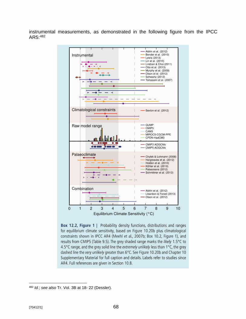
[70412/1] 68

instrumental measurements, as demonstrated in the following figure from the IPCC AR5:482

482 Id.; see also Tr. Vol. 3B at 18- 22 (Dessler).

[70412/1] 69

240. Pointing to the annotation in the above figure, the Agencies noted that the gray shaded area represents the likely 1.5 to 4.5oC range of ECS and the gray solid line represents the extremely unlikely ECS of less than 1oC. The Agencies concluded that the available evidence, as represented by the IPCC AR5, does not support Peabody’s assertions regarding ECS. 483

241. The CEOs addressed the question of why the IWG chose not to adopt the IPCC’s updated ECS values in the 2013 FSCC updates, quoting from the IWG’s 2015 Response to Comments:484

The IWG is aware that this is an active area of research and remains committed to updating the SCC estimates to incorporate new scientific information and accurately reflect the current state of scientific uncertainty regarding the ECS. While we agree with commenters that the ECS distribution, along with other climate modeling inputs to the SCC calculation, should be updated periodically to reflect the latest scientific consensus, care must be exercised in selecting an appropriate range of estimates for this important parameter. Many studies estimating climate sensitivity have been published, based on a variety of approaches (instrumental record, paleoclimate observations, models, etc.). These individual studies report differing values and provide different information. Picking a single study from the high or low end of the range, or even in the middle, will exclude relevant information. A valid representation of uncertainty regarding climate sensitivity should be obtained from a synthesis exercise such as that done by the IPCC that considers the full range of relevant studies. At the time the 2013 SCC update was released, the most authoritative statement about ECS appeared in the IPCC’s AR4. Since that time, as several commenters noted, the IPCC issued a Fifth Assessment Report that updated its discussion of the likely range of climate sensitivity compared to AR4. The new assessment reduced the low end of the assessed likely range (high confidence) from 2°C to 1.5°C, but retained the high end of the range at 4.5°C. Unlike in AR4, the new assessment refrained from indicating a central estimate of ECS. This assessment is based on a comprehensive review of the scientific literature and reflects improved understanding, the extended temperature record for the atmosphere and oceans, and new estimates of radiative forcing.

483 Ex. 803 at 18 (Gurney Rebuttal). 484 Ex. 101 at 45-46 (Polasky Rebuttal).

[70412/1] 70

Several of the post-AR4 studies highlighted by some commenters were cited in the AR5 assessment. In particular, both Aldrin et al. (2012) and Otto et al. (2013) were cited in both Chapter 10 and Chapter 12 of the AR5 Working Group I assessment. Eight of the authors of Otto et al. (2013), including the lead author, were authors of Chapter 12 for AR5’s Working Group I and one was a lead author for the chapter. Hence it is clear that the IPCC considered Otto et al. (2013) in its synthesis of literature on the ECS. More broadly, the AR5 climate sensitivity distribution likely incorporates much of the literature identified by the commenters. The IWG will continue to follow and evaluate the latest science on the equilibrium climate sensitivity and seek external expert advice on the technical merits and challenges of potential approaches prior to updating the ECS distribution in future revisions to the SCC estimates, including (but not limited to) using the AR5 climate sensitivity distribution for the next update of the SCC.

242. The CEOs’ witness, Dr. Dessler, stated that the IPCC AR5 relied heavily on 20th Century observational records. Many of the world’s experts in climate sensitivity have since agreed that the 20th Century observational estimates have previously unrecognized methodological problems which result in incorrect ECS estimates. As a result, Dr. Dessler asserted that if the IPCC ECS estimate were to be reassessed today, the lower bound would likely again be 2 degrees instead of the 1.5 degrees published in the AR5.485

243. The CEOs concluded that the IWG’s approach to climate sensitivity is a reasonable one.486

E. Marginal Ton: last unit of CO2 emitted

1. Criticisms

244. The Agencies explained that the IAMs’ damage functions are generally convex until temperature increases grow quite substantial. Consequently, every additional unit of CO2 emitted causes more damage than its predecessors. Damages are caused by the total quantity of CO2 in the atmosphere.487 The Utilities and MLIG contended that the IWG’s decision to value more recent CO2 emissions as though they are more damaging than earlier CO2 emissions is inappropriate.488 Rather, the Utilities and MLIG argued that the damages caused by CO2 in 2020 will consist of damages caused that year plus damages in all future years.489 The Utilities and MLIG explained:

485 Tr. Vol. 3A at 111-112 (Dessler). 486 Ex. 101 at 46 (Polasky Rebuttal). 487 Ex. 801 at 49-51 (Hanemann Rebuttal). 488 Ex. 300 at 15 (Smith Direct). 489 Id. at 20.

[70412/1] 71

[M]any of the tons emitted that contribute to the SCC will not be emitted until much later than the Minnesota tons in question. For example, the SCC value for 2020 depends on the concentration of greenhouse gasses projected to already exist by 2020, all emissions produced in 2020, and all emissions produced from 2020 into the far future.490

245. The Utilities and MLIG explained “the ‘marginal’ damage of an incremental amount of emissions reduction should be equal to the ‘marginal’ or incremental societal cost to accomplish that reduction.”491 That is why economists focus on marginal damages when they estimate the value of environmental externalities. How much of a pollutant is emitted is key to establishing the marginal damage. With GHGs, the marginal damage estimate depends on the baseline underlying the projected emissions. The marginal damage will be higher if the baseline reflects a world with no established GHG control policies, as opposed to a world with global GHG controls.492

246. The IWG’s methodology for calculating the FSCC is to use the socioeconomic scenarios to establish a baseline of damages and then subtract the baseline from the damages resulting from an additional unit of CO2. The IWG’s marginal damage estimate thus depends on the baseline scenarios. The Utilities’ and MLIG’s concerns were heightened because, they claimed, “the IWG has assumed no reductions in greenhouse gases other than the ton in question . . . .”493 This caused marginal damages to be higher than they would be if policies to restrict emissions were in place.494

247. The Utilities and MLIG disagreed with this result because an actual change in climate risk requires global action to achieve large reductions. Therefore, the Utilities and MLIG maintained, all emitters’ tons “that would remain under a global reduction plan should be valued like every other emitter’s tons, which suggests either a marginal damage estimate assuming the emissions are on the globally-controlled target trajectory, or an average damage of all the tons emitted.”495 The Utilities and MLIG also observed that, in the prior proceeding, the Commission adopted an average cost per ton approach.496

248. The Utilities and MLIG recommended two alternative marginal cost estimates, either of which, they asserted, would be preferable to the IWG’s marginal cost definition: (1) an estimate of the marginal cost halfway between the first and last tons, which the Utilities and MLIG called the average marginal cost value;497 or (2) baselines

490 Id. 491 Ex. 300 at 21 (Smith Direct). 492 Id. 493 Id. at 21-22. 494 Id. 495 Ex. 302, AES-D-2 at 7-8 (Smith Direct). 496 Id. at 8. 497 Ex. 308 at 3 (Smith Opening Statement); Tr. Vol. 2A at 58-60, 82-85 (Smith); see also Ex. 302, AES-D-2 at 8 (Smith Direct).

[70412/1] 72

in which there are no additional emissions of CO2 after the incremental emission. Either approach would lower the damage estimates compared to the IWG’s approach.498

249. Xcel agreed with the Utilities and MLIG that the IWG’s “last-ton” approach likely overstates damages from Minnesota emissions, and would similarly overstate the benefits that would accrue from an incremental reduction in emissions in Minnesota.499 Xcel supported the idea of the average ton approach in theory, but did not recommend it because it would not be practicable to implement.500

2. Responses

250. The Agencies criticized the first ton approach taken by the Utilities and MLIG because the first ton approach assumes that no anthropogenic emissions will occur after the year 2020.501 The year 2020 is the baseline scenario for the first ton approach, with an “emission blip on that baseline . . . .” which is then compared to damages with and without the 2020 blip.502 According to the Agencies, this is not a reasonable foundation on which to base an SCC.503 The Agencies argued that warming in any future year depends on emissions that occurred before the present as well as emissions that occur between now and the future date for which emissions and damages are being estimated.504

251. The CEOs contended the Utilities and MLIG’s discussion of what is meant by “marginal” damage is confusing and inconsistent with the way economists discuss marginal damage. They asserted that introductory economics instructs that the “efficient decision occurs where marginal cost equals marginal benefit, not where average costs equals average benefits, and certainly not where the cost of the first unit is equal to some measure of benefits.”505

252. The actual argument that the Utilities and MLIG have is not with the marginal ton or marginal damage, according to the CEOs, but “with the emissions projections from which marginal damage is calculated.”506

253. The CEOs distinguished between damages, which are the result of particular levels of emissions over time, and assumptions about emissions, which the Utilities and MLIG were making. Those assumptions were, with the “first ton” approach, that there would be no further emissions after 2020 because there is a global climate policy in place equating the marginal cost of reducing emissions with the SCC and determining the quantity of emissions resulting from this policy; or with the “average ton”

498 Ex. 300 at 48 (Smith Direct). 499 Ex. 601 at 46 (Martin Rebuttal). 500 Id. at 47. 501 Ex. 801 at 28 (Hanemann Rebuttal). 502 Id. 503 Id. at 29. 504 Id. at 28. 505 Ex. 101 at 10 (Polasky Rebuttal). 506 Id.

[70412/1] 73

approach, that an “average” amount of emissions could be predicted between zero and the IWG’s projections.507

254. The IWG stated “[t]here is a limited amount of research linking climate impacts to economic damages” making the IAMs’ analysis of that relationship difficult.508 Nonetheless, the CEOs emphasized that the IWG’s approach to calculating damages, based on a range of projections of emissions given likely future conditions, including future technology, economic and political circumstances, is the better approach and based on a current understanding of the likely potential trajectories of future emissions.509

F. Modeling Time Horizon: Estimates of damages after 2100

1. Criticisms

255. The Utilities and MLIG criticized the IWG for extending the IAMs’ time horizon to the year 2300.510 The EMF-22 scenarios were not constructed to allow calculations beyond the year 2100.511 The Utilities and MLIG asserted that the extension of the scenarios to 2300 required the IWG to make assumptions so speculative and uncertain that they are inconsistent with the Commission’s standard established in the 1993 Externalities docket.512

256. Up to about 3 degrees centigrade, the Utilities and MLIG acknowledged there is some limited empirical evidence about how climate change will impact the economy.513 By extending the time horizon of the scenarios, significant numbers of the IAMs’ runs project very high temperature increases. Because there is no data to support the amount of damages that will result from temperature increases over about 4 degrees centigrade, the Utilities and MLIG contended that much of the FSCC estimate is speculative.514

257. With decreasing discount rates, increasing portions of the FSCC values came from the post-2100 time period, according to the Utilities’ and MLIG’s calculations. For example, at a 5 percent discount rate, about one-quarter of the FSCC estimates come from the post-2100 era range. At a 3 percent discount rate, the Utilities and MLIG estimated that about one half of the FSCC consisted of damages incurred after 2100.515 The Utilities and MLIG found these values highly speculative.516

258. The Utilities and MLIG compared the IWG’s effort to predict the socioeconomic state of affairs in 2300 to that of a projection by someone in 1715 of

507 Id. at 10-11. 508 Ex. 100, Schedule 2 at 5 (Polasky Direct). 509 Ex. 101 at 12 (Polasky Rebuttal). 510 Ex. 300 at 15, 22-23 (Smith Direct). 511 Tr. Vol. 2A at 80-81 (Smith). 512 Ex. 300 at 15 (Smith Direct); 93-583 PUC ORDER 2 at 8. 513 Ex. 308 at 2 (Smith Opening Statement). 514 Ex. 302, AES-D-2 at 70-72 (Smith Direct). 515 Id. at 75-79. 516 Id. at 75-76.

[70412/1] 74

conditions today.517 In particular, the Utilities and MLIG criticized the IWG’s assumption that “future generations will passively endure temperature changes as high as 10° C above pre-industrial levels, without taking any steps whatsoever to address the causes of such temperature changes.”518 The Utilities and MLIG stated it is unreasonable for the IWG to assume that future generations will not develop new or improve existing technologies that would alter the relationships between population and GDP growth and CO2 emissions.519 The Utilities and MLIG noted there are numerous ways societies can undertake to reduce emissions as well as to promote carbon sequestration such as encouraging the planting of trees. The Utilities and MLIG noted that some of these reductions are incorporated into the PAGE and FUND models.520

259. The Utilities and MLIG pointed out the Commission adopted an estimate based on a time horizon of 100 years when it determined the social cost of carbon in 1997.521

260. Xcel expressed concerns about the great uncertainty in the EMF scenarios as they were extrapolated to the year 2300, asserting that the IWG inserted largely arbitrary assumptions into the scenarios in the years past 2100. In addition, Xcel contended that, even if the modeling assumptions were correct, predicting emissions required yet another layer of assumptions which were not based on evidence. Like the Utilities and MLIG, Xcel found the lack of endogenous modeling of societal response to emissions troubling. 522

2. Responses

261. The CEOs maintained that the impact of a unit of emission of CO2 should be taken into account for as long into the future as that CO2 is likely to remain in the atmosphere, causing damages.523 Because some estimates state that a unit of CO2, along with its associated warming effects, will remain in the atmosphere for up to 200 years, the CEOs asserted that it would be arbitrary to exclude some time period in the future where damages are likely to occur.524

262. Acknowledging that eventually the combination of a low probability that the unit of CO2 will remain in the atmosphere and the impact of discounting will make the value of future damages negligible, the CEOs agreed that the IWG appropriately determined that the year 2300 was the proper end point in time for purposes of calculating the FSCC.525

517 Ex. 300 at 22 (Smith Direct). 518 Id. 519 Ex. 302, AES-D-2 at 72-73 (Smith Direct). 520 PAGE and FUND “explicitly incorporate some assumptions regarding how adaptation may mitigate climate change impacts.” Ex. 302, AES-D-2 at 20 (Smith Direct). 521 Id. at 69. 522 Ex. 600 at 31-35 (Martin Direct). 523 Ex. 101 at 15 (Polasky Rebuttal). 524 Ex. 101 at 15; Schedule 1 at 29 (Polasky Rebuttal). 525 Ex. 101 at 15 (Polasky Rebuttal); see also Ex. 405 at 545 (IPCC AR5).

[70412/1] 75

263. The CEOs admitted that it is not possible to predict with great accuracy what will happen between now and 2300. But the CEOs alleged that it is also not possible to predict with great accuracy what will happen between now and 2140, 2100 or even 2050.526

264. The CEOs agreed with the Utilities and MLIG that making predictions to the year 2300 is filled with uncertainty. But the CEOs disagreed with the solution offered by the Utilities and MLIG, which was to assume that there would be zero damages after the year 2100 or 2140. The CEOs claimed such an approach “has no bearing in reality” and is not viable.527

265. The Agencies responded to the Utilities’ and MLIG’s concerns that the EMF-22 scenarios only go through 2100. The Agencies explained that the purpose of the EMF-22 scenarios, unlike the IWG’s purpose, was not a cost-benefit analysis of climate mitigation policies. Rather, the EMF-22 scenarios were focused on cost minimization in reducing emissions to meet targets being considered in current climate policy debates and focused on abatement costs to meet a specific goal in the year 2100. Damages were not considered in any other year, either before or after 2100.528

266. The Agencies maintained that the EMF-22 scenarios are projections and that the nature of projections is that they cannot be based on evidence or facts. They can only be based on reasonable assumptions. For that reason, the Agencies did not recognize a significant distinction between the EMF-22 scenarios as they were originally designed to project to the year 2100 and as the IWG extrapolated them to go to the year 2300. The Agencies understood both uses of the EMF-22 scenarios to be fairly similarly speculative.529

267. The Agencies pointed out that Xcel’s description of the IWG’s emissions scenarios projections was misleading because Xcel’s illustration of the IWG’s emissions scenarios ends at approximately 2100, leaving the impression that, with the exception of the fifth scenario, emissions will continue to rise.530 But, the Agencies observed, the IWG’s emissions scenarios projections level off and decline between 2150 and 2200.531 The Agencies noted that the IWG did not assume that emissions would continue to grow from 2100-2300. Instead, the IWG provided for societal response to climate change by placing a 20 percent weight on the fifth scenario emission projection that hypothesizes a global climate stabilization plan at 550 ppm of CO2.532

526 Ex. 101 at 16 (Polasky Rebuttal). 527 Ex. 101 at 16 (Polasky Rebuttal). 528 Ex. 801 at 24-25 (Hanemann Rebuttal). 529 Id. at 25. 530 Id. at 18-23. 531 Id. 532 Id. at 23. Dr. Hanemann explained that the goal of 550 ppm originated in the 1990s to define the concentration of CO2 that would cause roughly a doubling of the pre-industrial concentration and avoid more than a 2°C warming. According to Dr. Hanemann, by 2007 it had become clear that a concentration of less than 550 ppm would be required to avoid warming beyond 2°C. Id. at 23-24.

[70412/1] 76

G. Geographic Scope

1. Criticisms

268. The Utilities and MLIG argued that using a FSCC based on global damages rather than damages incurred by Minnesotans is inappropriate.533 They reasoned that Minnesota’s application of the FSCC in its resource planning efforts will not bind other states or nations to doing the same, and will have no significant impact on climate change.534

269. The Utilities and MLIG stated that Minnesota should not impose costs upon its residents that will be much greater than the benefits they will receive as a result of any emissions reductions.535 The Utilities and MLIG ran the FUND and PAGE models, limiting damages to those that will be experienced in the United States.536 The result “reduces the SCC by 81% to 84% from its value when global damages are considered.”537 Assuming that Minnesota’s damages are proportionate to its share of the United States’ GDP, the Utilities and MLIG alleged that Minnesota’s domestic-only SCC estimate would be lower by a factor of more than 50.538

270. MLIG argued that the CEOs failed to properly consider the definition of “society” when the CEOs defined the term “externality value” to “include[] the total external costs inflicted on society from the emission of pollution.” 539

271. MLIG framed the question of who should be counted in calculating “the external costs of pollution, or equivalently, the external benefits of reducing pollution” as a question of “economic standing.”540 In reviewing this cost-benefit analysis, MLIG discussed the issue in terms of who pays the costs of the policy of reducing pollution and who receives the benefits.541

272. MLIG advised that “standard benefit-cost analysis applied to a policy paid for by the residents of a state would evaluate the benefits to residents of the state rather than of neighboring states.”542

273. MLIG recognized that there are justifications for considering the benefits of residents outside the jurisdiction that would incur costs under the policy being considered.

533 Ex. 300 at 15 (Smith Direct). 534 Ex. 300 at 15, 27 (Smith Direct). 535 Id. at 36-37. 536 Ex. 302, AES-D-2 at 98 (Smith Direct). Dr. Smith did not include the DICE model in this analysis because it has no regional detail. Id. 537 Id. 538 Id. at 99. 539 Ex. 400, Appendix 2 at 3 (Gayer Direct). 540 Ex. 400, Appendix 2 at 3 (Gayer Direct). 541 Id. at 4. 542 Id.

[70412/1] 77

Those justifications include intergovernmental grants, an explicit recognition or expectation of reciprocity, or altruistic motivations, according to MLIG.543

274. MLIG advocated the use of a Minnesota, rather than a global, scope of damage calculation in the absence of express reciprocity. Alternatively, taking into account demonstrative feelings of altruism even in the absence of reciprocity, MLIG recommended a much narrower damages scope, such as United States damages.544

275. MLIG acknowledged that the IWG provided some estimates of the national domestic benefits of reducing CO2, but added that there was no effort to estimate the state-specific benefits of reducing CO2.”545

276. MLIG asserted that if the global approach to measuring the SCC were applied more broadly as a state policy, it “would demand a dramatic shift in all state policies, including state poverty programs.”546 MLIG suggested it would be important to consider what this “practice of granting benefits to non-residents equally to benefits of residents across the world would suggest if applied to all policies.” MLIG projected that the end result could mean that poor people all over the world would have equal standing to receive low-income assistance from Minnesota.547

277. Peabody distinguished the American Cost of Carbon from the global SCC. The American Cost of Carbon measures only the damages experienced in the United States and is about 5% of the global SCC.548 Peabody opined that Minnesota is “currently a net beneficiary of warming” because sea level rise and tropical cyclones do not affect Minnesota and “[a] warmer, wetter, CO2-enriched world would be a clear gain for Minnesota agriculture.”549

2. Responses

278. In response to the parties who urged the Commission to limit the scope of damages to the United States or to Minnesota, the Agencies reiterated their claim that GHGs are different from criteria pollutants in the spatial scale of their impacts.550 Because GHGs emitted in one location on earth mix with GHGs emitted from all other locations on the planet, each GHG molecule emitted contributes to climate change experienced everywhere. Consequently, the Agencies asserted, damages are experienced globally.551

279. The CEOs argued that a Minnesota electric power generating emitter must incorporate into the generator’s production decision process the damages its emissions 543 Id. at 5. 544 Ex. 400 at 9 (Gayer Direct). 545 Ex. 400, Appendix 2 at 15 (Gayer Direct). 546 Ex. 400 at 9 (Gayer Direct). 547 Ex. 400, Appendix 2 at 15-16 (Gayer Direct). 548 Ex. 214 at 3-4 (Mendelsohn Direct). 549 Id. 550 Ex. 801 at 13 (Hanemann Rebuttal). 551 Id.

[70412/1] 78

cause to all parties.552 To incorporate only Minnesota damages, asserted the CEOs, would be to ignore the vast majority of external costs.553 If every political territory only considered external damages within its own boundaries, the CEOs claimed that “there would be virtually no correcting for externalities.” While recognizing that some states may fail to take external damages into account in their decision-making, the CEOs stated that those states will be unprepared for future decision-making regarding climate change. By taking into account the full cost of CO2 externalities, the CEOs said Minnesota will be leading and “preparing for a future where the price of emitting carbon is no longer free.”554

280. The Agencies stated that the question of whether the geographic scope of CO2 emissions should be taken into account when determining the FSCC is a policy decision, rather than a matter of economic theory.555 The Agencies note that the Utilities and MLIG “appeared to agree” that this is a policy decision, although the Utilities and MLIG were critical of the IWG’s decision.556

281. The Agencies’ expert, Dr. Hanemann, believed it was most appropriate to defer to “precedent in Minnesota’s previous decisions regarding the environmental cost of electricity that bear on the policy decision involved here.”557 The expert asserted that the Agencies themselves, and the Commission, all state that a global scale of analysis is the proper approach to take to calculating the environmental cost of electricity.558

282. Xcel agreed that the geographic scope of damages is a policy decision for the Commission to make. Xcel remarked that, on one hand, the Commission may wish to demonstrate environmental leadership and to provide an example to encourage reciprocity even if implicitly.559 On the other hand, Xcel maintained, it is important to recognize the small contribution to emissions and climate change that Minnesota makes, even in relation to the United States. Xcel pointed out that, if Minnesota adopts a SCC based on global damages, any resulting resource planning decisions, even if they lead to a complete elimination of CO2 emissions in Minnesota, would have a small impact on global climate damages or on damages experienced by Minnesotans.560 Xcel noted that its own proposal could be adjusted if the Commission chooses to base the SCC on United States or Minnesota damages rather than the global damages reflected in the FSCC numbers.561

552 Ex. 101 at 26 (Polasky Rebuttal). 553 Id. 554 Ex. 101 at 26 (Polasky Rebuttal). 555 Ex. 801 at 15 (Hanemann Rebuttal). 556 Id. 557 Id. 558 Id. at 16. 559 Ex. 601 at 39 (Martin Rebuttal). 560 Id. Xcel linked these concerns to its concerns about leakage, discussed in Section IV.H of this Report. Xcel encouraged the Commission to consider the wider impacts leakage might have on its customers, and in this docket, or a separate docket, to consider ways in which such impacts might be mitigated. Id. at 39-40. 561 Ex. 602 at 6 (Martin Surrebuttal).

[70412/1] 79

283. Specifically responding to MLIG’s expert, Dr. Gayer, the CEOs emphasized that Gayer focused on the economic standing of “who is to be counted in the calculation of the external costs of pollution, or, equivalently, the external benefits of reducing pollution.”562 In response to Gayer’s query, the CEOs stressed that, because Minn. Stat. § 216B.2422 requires the Commission to “quantify and establish a range of environmental costs associated with each method of electricity generation,” economic standing belongs to “all parties damaged by the emission of a unit of CO2.”563

284. The CEOs disagreed with Dr. Gayer’s economic analysis that standard benefit-cost practice means considering only the benefits for the residents of that political jurisdiction who are bearing the costs of the policy being considered. The CEOs regarded externalities as a market failure, an attempt to reduce damages that Minnesota activity is inflicting on others.564

285. The CEOs rejected Dr. Gayer’s suggestion that the FSCC’s global damages approach would require reconsideration of state poverty policies. The CEOs asserted that Dr. Gayer’s comment in this regard conflates two unrelated issues.565

286. The CEOs reported that the IWG addressed the issue of global damages in its July 2015 Response to Comments. The CEOs noted that “because GHG emissions are a global problem they set up a classic public goods, or tragedy of the commons, scenario: ‘[I]f all countries acted independently to set policies based only on the domestic costs and benefits of carbon emissions, it would lead to an economically inefficient level of emissions reductions which could be harmful to all countries, including the United States, because each country would be underestimating the full value of its own reductions.’”566 The CEOs asserted that the same reasoning applies to Minnesota as a state.567

H. Leakage

1. Criticisms

287. The Utilities and MLIG explained that leakage occurs when reduced CO2 emissions in one jurisdiction are replaced by increased CO2 emissions in another jurisdiction.568 “Leakage is the extent to which policy-driven decreases in carbon emissions are offset by resulting increases in other jurisdictions.”569

288. The Utilities and MLIG pointed out that Minnesota’s electrical grid is interconnected to electricity systems in other states that may not impose equivalent costs on carbon emissions. As a result, the Utilities and MLIG reasoned, the use of an SCC in 562 Ex. 101 at 26 (Polasky Rebuttal). 563 Ex. 101 at 27 (Polasky Rebuttal). 564 Id. at 27-28. 565 Id. at 28. 566 Id. at 28-29. 567 Ex. 101 at 29 (Polasky Rebuttal). 568 Ex. 300 at 27 (Smith Direct). 569 Id. at 27-28.

[70412/1] 80

resource planning in Minnesota will result in fewer CO2 emissions in Minnesota but additional CO2 emissions elsewhere to meet electrical demand.

289. According to the Utilities and MLIG, the “net” impact on emissions is the emissions reduction in Minnesota less the amount by which emissions increase elsewhere to supply the demand for electricity in Minnesota.570

290. The Utilities and MLIG supported the consideration of leakage when using CO2 environmental cost values.571 However, they would not take leakage directly into account in calculating the SCC. Instead, they would apply SCC values to a net total ton of CO2 emissions, after applying a calculated leakage amount in each particular resource planning situation.572

291. The Utilities and MLIG described a method to estimate leakage. Specifically, a detailed generation planning model of the Minnesota electric system and the power pools that connect to Minnesota can be run with and without a specific change in generation resources in Minnesota.573 “The ratio of the change in emissions outside Minnesota to the change in emissions within Minnesota would yield the amount of estimated leakage.”574 Such a model can be run with and without a specific change in generation resource in Minnesota (and hence a specific direct change in Minnesota’s electricity sector CO2 emissions). The ratio of the change in emissions within Minnesota would yield the amount of estimated leakage.”575

292. The Utilities and MLIG alleged the rate of leakage can be as high as nearly 100 percent if a state takes an action and the region is not imposing similar policies.576 The Utilities and MLIG argued that estimated leakage should be accounted for because the SCC should only be applied to the net emissions reduction estimates.577 Further, the IWG did not account for leakage in its computation of the FSCC values.578 The Utilities and MLIG asserted that to arrive at a net change in metric tons, the direct CO2 reduction estimates associated with resource planning should subtract an estimate of potential increases in metric tons occurring outside of the Commission’s jurisdiction.579

293. The Utilities and MLIG stopped short of making a specific recommendation for a leakage value to consider because it will vary based on the decision under consideration. But, they assert, whatever CO2 environmental cost values the

570 Ex. 300 at 27-28 (Smith Direct). 571 Id. at 28. 572 Id. at 34. In her oral testimony, Dr. Smith noted that the IWG acknowledged in its response to comments that SCC values from the federal government should be applied to the number of tons as adjusted for leakage. Tr. Vol. 2A at 106 (Smith). 573 Ex. 302, AES-D-2 at 100 (Smith Direct). 574 Id. 575 Id. at 102. 576 Id. at 100; see also Tr. Vol. 2A at 102 (Smith). 577 Ex. 300 at 29 (Smith Direct). 578 Id. 579 Id. at 34.

[70412/1] 81

Commission adopts should be adjusted by the estimated level of leakage.580 The higher the dollar per ton of CO2, the greater the likelihood that leakage will be a problem and the benefit of that externality value would be reduced.581 The Utilities and MLIG noted that it would be easier for manufacturing to decide to move across state boundaries if higher utility prices were triggered in Minnesota.582

294. Even if a new generating unit were built in Minnesota, the Utilities and MLIG warned that leakage could still occur if the replacement unit were to have more expensive fuel or be intermittently dispatched, if the new generation is wind or solar. Therefore, they maintained, the potential for leakage is significant and should be closely analyzed. 583

295. The Utilities and MLIG urged the Administrative Law Judge to recommend that the Commission adopt an estimate of the SCC net of leakage in this proceeding and that the Commission conduct a leakage study “as part of any application of the CO2 environmental cost values that result from this proceeding.”584

296. MLIG’s witness, Dr. Gayer, supported the Utilities’ and MLIG’s witness, Dr. Smith, in her suggestion to apply the SCC to the net reduction in emissions.585 MLIG did not agree with the Agencies’ premise that leakage should not be considered because Minnesota only regulates utilities within Minnesota.586 MLIG maintained that if Minnesota ignores leakage and emissions are increased elsewhere as a result, the regulation would not serve its purpose.587

297. MLIG urged the Commission to take leakage seriously and to consider leakage if the SCC is applied inconsistently across states, or Minnesota’s regulation would be undermined.588 Unless the SCC is applied across different countries, MLIG disagreed with the CEOs’ view that leakage does not affect the externality value the Commission adopts.589 At least conceptually, MLIG warned that there could be more harm to the environment through leakage if Minnesota adopts a high SCC.590 The goal should be to reduce emissions and not simply to price emissions, cautioned MLIG.591

298. Peabody emphasized that it is critical that the amount of leakage be calculated and included in the final SCC calculation.592 Disagreeing with the Agencies, the CEOs, Xcel and the Utilities, Peabody contended that leakage should be considered

580 Id. at 40. 581 Tr. Vol. 2A at 103, 105 (Smith) 582 Ex. 302, AES-D-2 at 101 (Smith Direct). 583 Id. at 102. 584 Id. at 49. 585 Ex. 401 at 10-11 (Gayer Surrebuttal). 586 Id. 587 Id. 588 Id. at 9-10. 589 Id. 590 Id. 591 Id. 592 Ex. 220 at 33 (Mendelsohn Surrebuttal).

[70412/1] 82

as part of Minnesota’s SCC given that the Commission is trying to determine what value to place on gross, and not net, carbon emissions.593

299. Peabody asserted that if Minnesota adopts a high price for CO2, rates will increase for Minnesota residents who “would be lucky if they get 1% of the benefits of this costly program” at best due to leakage if neighboring states and countries do not adopt similar policies and prices.594

300. Peabody argued that the greater the difference in CO2 cost in Minnesota compared to the rest of the region, the greater the leakage will be.595 Due to leakage, emissions would be simply reassigned, not reduced.596 For example, if Minnesota insists that imported power be based on low carbon fuels, neighboring states may assign natural gas generation to the Minnesota market and respond by increasing generation from coal plants for their own markets.597 Additionally, Peabody speculated that if Minnesota had high prices as a result of a high CO2 cost, surrounding states could lure businesses from Minnesota to avoid higher prices.598

2. Responses

301. The Agencies asserted that leakage should not be considered when applying a SCC value.599 The Agencies reasoned that, because the Commission regulates utilities that operate in Minnesota and does not have jurisdiction in other states or countries, the Commission has no responsibility for the aggregated level of emissions resulting from other jurisdictions’ action or inaction.600 The Agencies found no reason for the Commission to modify its assessment of an environmental cost based on what may or may not happen in other jurisdictions.601

302. The CEOs explained that leakage does not affect the CO2 values adopted by the Commission and did not support the consideration of leakage when calculating the FSCC values.602

303. The CEOs explained that leakage is a policy issue that can be addressed through other Commission actions and agreed with the IWG’s response to leakage questions.603 The IWG is concerned with leakage, but not as leakage affects the calculation of damages.604 The FSCC is an estimate of the marginal benefit of a net one-

593 Id. 594 Ex. 218 at 3 (Mendelsohn Rebuttal Ex. 1). 595 Ex. 220 at 33 (Mendelsohn Surrebuttal); Tr. Vol. 3B at 42-43 (Mendelsohn). 596 Ex. 218 at 4 (Mendelsohn Rebuttal Ex. 1). 597 Id. at 3-4. 598 Ex. 214 at 5 (Mendelsohn Direct). 599 Ex. 801 at 30 (Hanemann Rebuttal). 600 Id. 601 Id. at 30-31. 602 Ex. 101 at 29 (Polasky Rebuttal). 603 Id. at 29-30. 604 Ex. 101 at 30; Schedule 1 at 32-33 (Polasky Rebuttal).

[70412/1] 83

ton reduction in CO2 emissions.605 The IWG explained that “[t]he FSCC estimates are multiplied by estimates of net GHG emissions changes to calculate the value of benefits associated with a policy action in a given year.”606 The CEOs concluded that the FSCC assigns a damage cost to emissions.607 The CEOs reasoned that the FSCC number assigned to the damages from a ton of carbon is not a function of leakage.608

304. Xcel also noted that the IWG recommends that any estimate of leakage be applied to emission reductions and not to the SCC itself.609 Xcel agreed with MLIG and the Utilities that the Commission could consider leakage in another proceeding because leakage is outside the scope of this proceeding, which is intended to determine damage cost values.610

305. Xcel disagreed with the Agencies’ argument that the Commission should not account for leakage when applying its CO2 cost range because the Commission lacks jurisdiction over utilities outside of Minnesota.611 Additionally, Xcel noted, the benefit of avoided climate damages may be overestimated if it ignores the possibility of leakage.612 In order to derive the value of climate damages avoided by Commission action, Xcel supported the Commission making a case-by-case estimate of leakage in a separate proceeding to derive an adjustment factor that would be multiplied by emission reductions in Minnesota, and then by Xcel’s proposed CO2 environmental cost range.613

306. Xcel suggested that an increase to the existing CO2 externality value would not likely by itself lead to a retirement of a coal-fired generation unit, but would be one of many considerations.614 In addition, Xcel noted that generation from a coal-fired generation unit could be offset with renewable energy.615 However, in a regional system such as Midcontinent Independent System Operators (MISO), Xcel maintained that generation from outside Minnesota could result in a net increase in emissions if retired generation in Minnesota is replaced by higher-carbon-emitting generation on a per-MWh basis outside of Minnesota.616

307. Xcel agreed with the Utilities and MLIG that it is not appropriate to adjust the SCC itself because leakage affects the total emission reductions.617 Xcel also agreed with the Utilities and MLIG that the amount of leakage will vary depending on what value

605 Ex. 101, Schedule 1 at 33 (Polasky Rebuttal). 606 Id. 607 Ex. 101 at 30 (Polasky Rebuttal); Tr. Vol. 1 at 126 (Polasky). 608 Tr. Vol. 1 at 126-127 (Polasky). 609 Ex. 601 at 52 (Martin Rebuttal). 610 Ex. 602 at 39-40 (Martin Surrebuttal); Tr. Vol 4 at 14-16 (Martin). 611 Ex. 602 at 39 (Martin Surrebuttal). 612 Id. 613 Ex. 601 at 53 (Martin Rebuttal); Tr. Vol. 4 at 43 (Martin). See discussion of Xcel’s proposed SCC cost range at section VII below. 614 Tr. Vol. 4 at 14 (Martin). 615 Ex. 601 at 53 (Martin Rebuttal); Tr. Vol. 4 at 15 (Martin). 616 Ex. 601 at 52-53 (Martin Rebuttal). 617 Id. at 53.

[70412/1] 84

the Commission assigns to CO2.618 Xcel explained that if leakage led to retirements of generation from fossil fuels, then leakage would be “fairly substantial and immediate” in the near term if that generation is replaced from elsewhere in the MISO system.619 However, if the CO2 environmental cost values motivate the addition of new zero-emissions generation, such as wind generation, the wind generation would be dispatched first by MISO, resulting in less leakage.620 Due to the de minimis nature of Minnesota’s emissions compared to the rest of the world, Xcel posited that there will likely be little reduction in global CO2 damages and, therefore, little reduction in CO2 damages for Minnesotans.621

I. Uncertainty

1. Criticisms

308. Peabody noted that, according to the CEOs, estimates of climate change impacts are incomplete and understated. However, Peabody asserted, the IWG models “include all impacts for which a global impact estimate is available.”622 Because the size and sign of uncounted impacts is not known, Peabody argued that the CEOs’ claim that missing impacts are significant and negative is speculative.623

309. Peabody also argued that the IWG’s use of Monte Carlo calculations in running the FSCC does not counter the uncertainty created by the IWG’s use of “ill-founded assumptions and arbitrary inputs” when it ran the IAMs. As examples, Peabody reiterated that the IWG’s ECS assumptions were likely biased high, and that the IWG failed to incorporate the environmental benefits of carbon dioxide.624

310. The nature of IAMs, according to Peabody, is such that they contain uncertainty at each step of the process. Peabody described the IAM process as magnifying uncertainties from step to step, creating a “cascade of uncertainties” that even techniques such as the Monte Carlo analysis and random simulation cannot significantly cure.625

311. Peabody criticized the IAMs’ use of probability distributions to compensate for the IAMs’ questionable damage functions. This use of a range of values around a norm “serves to acknowledge that we have no real scientific evidence to support one value over another – their use introduces another bias into the IAM results. Since the structure of the damage functions are quadratic equations, the results of using probability

618 Id. 619 Id. 620 Ex. 601 at 53 (Martin Rebuttal); Tr. Vol. 4 at 15 (Martin). 621 Ex. 601 at 28 (Martin Rebuttal). 622 Ex. 238 at 8 (Tol Rebuttal Ex. 2). 623 Id. 624 Ex. 242 at ¶ 30 (Wecker Rebuttal Ex. 2). 625 Ex. 230 at 110-111 (Bezdek Direct Ex. 2).

[70412/1] 85

distributions of equation parameters results in so-called ‘fat-tail’ impacts that are larger for higher increases than for lower increases.”626

312. Xcel asserted that the IWG had to make inherently uncertain policy judgments and establish uncertain scientific parameters when estimating climate change damages to the year 2300.627

313. Xcel acknowledged that the IWG attempted to address the inherent uncertainty regarding climate change in several ways, including using three IAMs, five different socioeconomic and emissions projections, a probability distribution for ECS, and three different discount rates. Despite the FSCC’s flaws, Xcel determined that it could be used as the basis for developing CO2 environmental cost values.628 However, Xcel found the FSCC’s approach of recommending four single point values rather than a range of values to give the impression of false precision. Therefore, based on the numbers calculated by the IWG, Xcel made its own proposal for establishing an SCC in this proceeding, which yielded a range of values.629 Xcel’s proposal is described at section VII, below.

314. Xcel quoted Professor Robert Pindyck on ECS uncertainty:630

We know very little about climate sensitivity, i.e., the temperature increase that would eventually result from a doubling of the atmospheric CO2 concentration, but this is a key input to any IAM. The problem is that the physical mechanisms that determine climate sensitivity involve crucial feedback loops, and the parameter values that determine the strength (and even the sign) of those feedback loops are largely unknown, and are likely to remain unknown for the foreseeable future. As Freeman, Wagner and Zeckhauser (2015) have shown, over the past decade our uncertainty over climate sensitivity has increased.

315. The Utilities and MLIG observed that there may be more scientific confidence now than in the 1990s that CO2 emissions will lead to climate change and resultant damages, and some IAMs now try to quantify higher risk outcomes connected with temperature increases that are higher than 2.5 degrees centigrade. Nonetheless, the Utilities and MLIG noted, the damage functions in the IWG’s IAMs are still based on limited empirical evidence.631

316. The Utilities and MLIG expressed strong concerns about the attempt to calculate damages over a four-degree centigrade increase or “after about 100 years from

626 Ex. 234 at 81 (Bezdek Rebuttal Ex. 2). 627 Ex. 600 at 5 (Martin Direct). 628 Id. at 52. 629 Id. 630 Id. at 39. 631 Ex. 300, AES-D-2 at 7 (Smith Direct).

[70412/1] 86

the present” as highly speculative.632 The Utilities and MLIG maintained that the damage functions in the IWG’s IAMs create an inaccurate appearance of knowledge and precision about CO2 emissions reduction benefits. This inaccuracy contributes to the overall uncertainty of the FSCC.633 The Utilities and MLIG asserted that the IWG failed to analyze the uncertainty in the FSCC resulting from the damage functions in the IAMs.634 The Utilities and MLIG structured their alternative assumptions for estimating the SCC values to counter the uncertainties resulting from the IWG’s IAMs’ damage functions.635

317. MLIG acknowledged that uncertainty does not justify inaction. However, MLIG cautioned that the uncertainty of a prediction “approaches infinity as time increases indefinitely.” Noting that the Congressional Budget Office has recently shifted its focus towards the first 25 years of its 75-year projections, MLIG maintained that “there is a point at which uncertainty gets so large that it makes the forecast useless and not worth basing current policy on.”636

2. Responses

318. The Agencies explained that the IWG acknowledged the scientific uncertainty that exists regarding climate sensitivity by making the ECS value a random variable in the IAMs with the same probability distribution for each of the models.637 The CEOs pointed out that ranges of values were selected for global projections of CO2 emissions and for discount rates and applied to all three IAMs to account for uncertainty concerning those inputs. 638

319. The Agencies noted that the use of probability distributions for the numerical value of certain parameters in FUND and PAGE is intended to account for the uncertainty regarding the value of those parameters.639 The Agencies further explained that PAGE contains ten random parameters and FUND contains eleven such parameters.640

320. The Agencies acknowledged that the Pindyck quotation cited by Xcel (see paragraph 314, above) was accurate in that uncertainty over climate sensitivity has increased.641 However, the Agencies argued that Dr. Pindyck’s concerns are not a persuasive argument against the Commission’s adoption of the FSCC.642 Asserting that Xcel failed to point out the implication that Freeman, Wagner, and Zeckhauser drew from this increase in uncertainty, the Agencies explained that the economic implication of the

632 Id. at 11. 633 Ex. 302, AES-D-2, Att. 1 at 5-6 (Smith Direct). 634 Id. at 8-9. 635 Ex. 300 at 33 (Smith Direct). 636 Ex. 401 at 12-13 (Gayer Surrebuttal). 637 Ex. 800 at 46 (Hanemann Direct). 638 Ex. 100 at 8 (Polasky Direct). 639 Ex. 800 at 42, fn 32 (Hanemann Direct). 640 Id. at 52. 641 Ex. 801 at 31-32 (Hanemann Rebuttal). 642 Id.

[70412/1] 87

increase in the uncertainty regarding climate sensitivity is that it raises the SCC in Pindyck’s economic model of climate change.643

321. The Agencies criticized the Utilities and MLIG for their failure to acknowledge the uncertainties regarding the location in time of climate tipping points and how such tipping points could affect the SCC. The Agencies drew an analogy to a bicyclist racing downhill, with an unknown curve ahead. The Agencies assumed that a good cyclist would brake until he determined how the curve should be handled. Similarly, the Agencies argued: 644

The existence of an uncertain threshold for a tipping point lying ahead is shown to raises [sic] the current SCC value. Once the tipping point danger is resolved, the SCC value drops down. This overturns the conventional pattern in which the SCC starts out low and rises over time: with tipping point uncertainty, the SCC would start out high.

322. The Agencies explained that the 2.5 percent discount rate was included in the FSCC to account for the concern that interest rates are quite uncertain over time.645

323. The CEOs recognized that uncertainty plays a major role in the process of estimating the SCC, and explained that the IWG dealt with uncertainty by using estimates from multiple IAMs and using a range of parameters in the models as described above.646 The CEOs emphasized that uncertainty is no excuse for inaction, or for assigning a value of zero for the SCC, but called for moving forward with the best information available in order to insure against the most catastrophic damages. The CEOs recommended adjusting the SCC in the future, as better information becomes available.647

J. Adaptation and Mitigation

1. Criticisms

324. Peabody agreed with MLIG that the IWG’s assumption of zero abatement in the future is incorrect.648

325. Peabody asserted that, because climate change is a very slow process, it is uncertain what it will look like fifty years from now but it is likely that “[i]f climate is not a surprise and it has important impacts, it is very obvious that people will react.” Peabody states that human adaptation will “substantially reduce damage.”649

643 Id. at 33. 644 Ex. 801 at 59-60 (Hanemann Rebuttal). 645 Id. at 86. 646 Ex. 100 at 8, 16 (Polasky Direct). 647 Id. at 16. 648 Ex. 214 at 15-16 (Mendelsohn Direct). 649 Ex. 220 at 18-19 (Mendelsohn Surrebuttal).

[70412/1] 88

326. Peabody argued that, even if the IWG’s ECS value of 3 is correct, it will take until the year 2100 for the climate to warm three degrees, assuming no attempts are made at abatement or mitigation. That will allow people time to adapt to moderate warming.650

327. The Utilities and MLIG pointed out that this proceeding demonstrates that it is not realistic to assume that society will passively allow damaging changes in the climate to occur without taking mitigating action.651

328. Xcel, and the Utilities and MLIG maintained that none of the IAMs incorporates, endogenously, any societal response to temperature and climate changes. Therefore, once the emissions trajectory is fixed, the IAMs presume that future societies do nothing beyond what is reflected in the emissions scenarios to mitigate even dramatic projected damages.652 In relation to this concern, Xcel invoked the Utilities’ and MLIG’s argument that one difficulty with projecting to the year 2300 is that attempting to model climate damage and society’s responses “out to the year 2300 is equivalent to scientists in the early 1700s attempting to model our society today.”653 In addition, the Utilities and MLIG asserted that projections of a society unresponsive to climate change in the future are particularly unrealistic given the likelihood, based on the IWG scenarios, that global society will be three to five times wealthier by 2100, and between seven and 25 times wealthier by 2300.654

329. Xcel agreed with Peabody, the Utilities and MLIG that the IWG’s “last ton” marginal damages approach unrealistically presumes no further actions will occur in the future to reduce emissions, resulting in an overstatement of the FSCC.655

330. Xcel also argued that, while the 95th percentile value captures some of the uncertainty of “tipping point” damages, it fails to account for the counterbalancing adaptation and technological change.656

331. The Utilities and MLIG recommended that instead of taking a risk management approach that attempts to value CO2 damage per ton using IAMs, Minnesota should recognize that a policy that “characterizes the more severe outcomes and experts’ best estimates of their probabilities is what is required to motivate action.”657 The Utilities and MLIG recommended balancing decisions on spending resources on incremental emissions reductions now with decisions to fund research and other investments to create future technologies and infrastructure “that will be better able to mitigate the impacts of worst-case outcomes.”658

650 Ex. 206 at 11 (Happer Surrebuttal). 651 Ex. 300 at 22 (Smith Direct). 652 Ex. 601 at 24-25 (Martin Rebuttal); see also Ex. 302, AES-D-2 at 74 (Smith Direct). 653 Ex. 601 at 25 (Martin Rebuttal). 654 Ex. 302, AES-D-2 at 74 (Smith Direct). 655 Ex. 601 at 46 (Martin Rebuttal). 656 Id. at 22. 657 Ex. 304 at 13 (Smith Surrebuttal). 658 Id.

[70412/1] 89

2. Responses

332. The Agencies agreed with Xcel that some adaptation and technological change will occur in the future. But, because the degree to which they will occur is not known, the Agencies could not say how such adaptation can be incorporated into the IAMs. In addition, the Agencies presumed that adaptation and technological change will not occur without cost. The Agencies also expressed strong doubts that any adaptation or technological change can counterbalance the uncertainty regarding catastrophic damages due to climate change.659

333. The Agencies pointed out that the IWG does account for mitigation, noting that one of its emissions scenarios stabilizes CO2 at 550 ppm by 2100.660 The Agencies also noted that mitigation activity is not unique to Minnesota, as demonstrated by the fact that the FSCC was developed to value federal mitigation efforts.661

334. The Agencies also questioned the Utilities’ and MLIG’s predictions about mitigation, given the time lag “before the effects of today’s transmissions are translated into future warming” and the concern that global CO2 reduction is an exercise in global collective action, which can be fraught with difficulties.662

335. The CEOs criticized the Utilities and MLIG for altering the models to assume zero emissions of CO2 after 2020.663

K. Use of FSCC Outside of Regulatory Setting

1. Criticisms

336. Several parties criticized the use of the FSCC as a state tool for resource planning, arguing that it was developed by the IWG so that federal agencies could include relevant cost-benefit analyses for proposed GHG emissions regulation in their Regulatory Impact Analyses as required by Executive Order 12866.664

337. The Utilities and MLIG asserted that the different purpose for which the FSCC is proposed to be used in Minnesota requires different framing assumptions, which have not been defined by the Agencies.665 The framing assumptions the Utilities and MLIG found inappropriate for Minnesota’s use, as discussed throughout this Report, are the “last ton emitted” approach to calculating damages, the modeling time horizon to 2300, the discount rates of 2.5 percent and nothing above 5 percent, the global scope of

659 Ex. 802 at 34 (Hanemann Surrebuttal). 660 Id. at 7. 661 Id. 662 Ex. 801 at 26 (Hanemann Rebuttal). 663 Ex. 101 at 14 (Polasky Rebuttal). 664 Ex. 302, AES-D-2 at 32 (Smith Direct); Ex. 601 at 20 (Martin Rebuttal); Ex. 400, Att. 2 at 6 (Gayer Direct). 665 Ex. 304 at 4-6 (Smith Surrebuttal). Dr. Smith talks about framing assumptions in the context of the FSCC as “certain key, non-scientific choices made by the modelers in framing their analysis.” Ex. 300 at 14 (Smith Direct).

[70412/1] 90

damages, and the failure to account for leakage.666 In addition, the Utilities and MLIG argued that the Commission “needs a principled way to evaluate the framing assumptions and choose which framing assumptions are appropriate to use in determining Minnesota’s” SCC.667

338. Xcel argued that the intended regulatory purpose of the FSCC allows for a “greater tolerance for the imprecise nature of the estimates, since a regulation would be warranted” as long as the cost-benefit analysis demonstrated that the benefits significantly outweigh the costs, even if the cost estimates are not precise.668 In contrast, Xcel claimed, in the resource planning context the FSCC would not be used to determine whether or not to adopt a regulation but “could drive specific, binary decisions that are not easy to reverse and have significant costs.”669

339. Xcel observed that attempts by the Agencies to conflate externality values with the CO2 regulatory cost range established pursuant to Minn. Stat. § 216H.06 (2014) are misleading. Xcel asserted that the Department and the CEOs have acknowledged that the regulatory cost range does not include damages, and so cannot serve as the basis for the CO2 externality value.670

340. In addition, Xcel noted that, in response to public comments, the IWG stated “that the SCC was developed for use in ‘cost-benefit analysis of regulation actions that have small, or marginal, impacts on cumulative global emissions.’ The IWG has not addressed the use of the SCC estimates outside the regulatory context, such as in . . . state-level decision-making, and ‘pricing’ carbon in the marketplace.”671

341. Xcel provided an illustrative analogy between the regulatory process with the Environmental Protection Agency’s (EPA’s) Clean Power Plan (CPP) to regulate CO2 emissions from existing power plants. Xcel maintained that, in developing the CPP, the EPA did not utilize the FSCC to determine which CO2 reduction measures “were feasible, cost-effective, or adequately demonstrated, nor was it relied on to determine how stringent the targets should be.” It was only after the regulations were developed that the EPA would have used the FSCC to determine whether the benefits of the CPP would likely outweigh its costs.672

666 Ex. 300 at 15 (Smith Direct). 667 Ex. 304 at 4 (Smith Surrebuttal). 668 Ex. 601 at 20 (Martin Rebuttal). 669 Id. 670 Id. at 21. 671 Id. 672 Ex. 602 at 7 (Martin Surrebuttal). The CPP is a set of EPA regulations authorizing GHG emission performance standards to apply to existing and, to a lesser extent, new power plant emissions sources. Under the CPP, states would be required to make GHG reductions by 2030 using various tools, including increased energy efficiencies, conservation investments, and emissions trading. As of the date of this Report, implementation of the CPP is stayed pursuant to an Order of the United States Supreme Court pending disposition of petitions for review in the Court of Appeals for the District of Columbia Circuit and possible petitions for a writ of certiorari. Chamber of Commerce et al. v. Environmental Protection Agency et.al, 136 S. Ct. 999 (Feb. 9, 2016).

[70412/1] 91

342. Xcel maintained that the FSCC in no way would have been involved in determining how states and utilities complied with the CPP and would not have established a carbon price for any state that chose to create a CO2 trading market. Xcel contrasted the impact of the way in which the FSCC is used at the federal regulatory level with its use as proposed in this proceeding – where using the FSCC for integrated resource planning “could potentially drive how to achieve CO2 reductions by driving resource choices, such as what to build and what to retire, that have significant customer cost impacts and are not easy to reverse.”673

343. Xcel concluded that the problem of the false precision associated with a single point value (or even four “single” points that are not a range) could lead to significant decisions being made by the Commission based on values with a false impression of precision.674

2. Responses

344. The Agencies reported that the Federal Department of Transportation has used the FSCC in the grant application context for documentation of benefits of proposed economic recovery projects. The Federal Railroad Administration requires use of the FSCC in high-speed rail grant applications to demonstrate reduced CO2 emissions. In addition, the Agencies asserted that the Federal Aviation Administration has a planning process that is similar to Minnesota’s integrated resource planning process in which the FSCC is used to estimate reductions in CO2 from alternative airport configurations, flight operations and routing and fuel composition. The Agencies also provided information regarding use of the FSCC in other venues, including: Canadian heavy-duty vehicle and engine GHG emissions regulations; a Montgomery County, Maryland county code on environment sustainability; and integrated resource planning processes used by energy providers in Washington, Oregon, Tennessee and Nevada. 675

345. The CEOs also responded to the criticisms that the FSCC is not meant to be used for the purpose of establishing a CO2 externality cost to be used in integrated resource planning. The CEOs asserted that, as an estimate of the external damages associated with CO2 emissions, the FSCC is applicable for a variety of purposes, including establishing a cost value for CO2 in this proceeding.676

346. The CEOs stated they found the “fundamental logic applied in cost-benefit analysis and integrated resource planning to be quite similar. Both . . . are tools that help inform decision-makers about the relative merits of . . . alternative choices.” The CEOs insisted that the FSCC is precisely the information the Commission requires to establish the external costs of CO2 emissions.677

673 Ex. 602 at 7-8 (Martin Surrebuttal). 674 Id. 675 Ex. 800 at 61- 62 (Hanemann Direct). 676 Ex. 101 at 33 (Polasky Rebuttal). 677 Id. at 34.

[70412/1] 92

347. The CEOs refuted the argument that IWG reported only a single value because it reported a value for each of three discount rates, along with the 95th percentile value at the three percent rate. The CEOs acknowledged that the Commission could adopt the full range of FSCC values across all three discount rates as well as the 95th percentile value to avoid the perception of false precision that Xcel raises. However, the CEOs also recommended that the three discount rate values generate a spread of values, with the 95th percentile value to address concerns about missing catastrophic damage costs.678

L. Whether the IWG Used a Scientific Process

1. Criticisms

348. Peabody asserted that the IWG process is neither peer-reviewed nor transparent.679 In addition, Peabody provided examples of non-peer-reviewed sources that witnesses for the CEOs, the Agencies and Xcel cited.680

349. Peabody disagreed with the CEO’s claim that 97 percent of the world’s climate scientists concur that humans are causing climate change.681 Peabody contended that science is based on evidence, not agreement, and that consensus should not be given any weight. Peabody provided examples of scientists, including Copernicus, Galileo, Einstein, and several contemporary scientists, who made significant breakthroughs in science despite being at odds with a majority consensus.682

350. Peabody also disagreed with the CEO’s claim that those disputing the premise that humans are causing climate change represent only a small minority of scientists.683 Peabody provided examples of other scientists who spoke against the understanding that the questions of whether climate change is occurring and is due to human activity are settled.684

351. Peabody disagreed with the Agencies’ description of the peer review process used by the IPCC and described in Finding 353, below.685 Peabody also disagreed with the Agencies’ assessment of the IPCC’s process as “two stringent layers of peer review,” but instead characterized the process as relying on a “closed ecosystem

678 Ex. 101 at 34-36 (Polasky Rebuttal). 679 Ex. 235 at 71 (Bezdek Surrebuttal); Ex. 213 at 51-52 (Lindzen Surrebuttal). 680 Ex. 235 at 71-80 (Bezdek Surrebuttal). Dr. Bezdek’s list of sources is lengthy, but only a few of the sources listed are part of the record in this matter. Also, Dr. Bezdek does not state where in the record the other witnesses allegedly rely on the cited sources. Thus it is difficult, if not impossible, to determine the accuracy of Bezdek’s allegations regarding whether the cited sources are peer-reviewed, and the context in which the sources were first published or presented. 681 Ex. 235 at 83 (Bezdek Surrebuttal); Ex. 238 at 9 (Tol Rebuttal Ex. 2); Ex. 213 at 46 (Lindzen Surrebuttal). According to Dr. Tol, the 97 percent figure “refers to the number of papers rather than the number of researchers.” Ex. 238 at 9 (Tol Rebuttal Ex. 9). 682 Ex. 235 at 83, 91-92 (Bezdek Surrebuttal). 683 Ex, 235 at 96 (Bezdek Surrebuttal); Ex. 213 at 47 (Lindzen Surrebuttal). 684 Ex. 235 at 96 (Bezdek Surrebuttal). 685 Ex. 213 at 50 (Lindzen Surrebuttal).

[70412/1] 93

of self-reinforcing voices.”686 Peabody pointed out that the IPPC relied on advocacy groups such as the World Wildlife Fund and Greenpeace for information. Peabody also pointed out that the CEOs, who support the IWG process, have themselves asserted that it is important to avoid relying on non-peer-reviewed material submitted by advocacy groups.687 Further, Peabody claimed that papers arguing for lower values for the SCC might be selectively omitted from published literature.688

352. Peabody alleged the IWG did not rely on the most relevant data and ignored all of the science published after 2007.689 Peabody argued that the most recent peer-reviewed literature is questioning the level of feedback mechanisms assumed by climate models and that Peabody’s expert, Dr. Happer, relied on peer-reviewed literature in his testimony.690 Peabody disputed the allegations by the Agencies that relying on laboratory studies weakens its argument that increased levels of CO2 enhance plant growth.691 According to Peabody, laboratory experiments are crucial for demonstrating biological mechanisms in place.692

2. Responses

353. The Agencies challenged Peabody’s claims regarding the scientific process as it applies to the IPCC, stating that the IPCC’s Assessment Reports are peer-reviewed and synthesize primarily peer-reviewed research, providing much of them with two layers of peer review.693 The Agencies acknowledged that papers can have conflicting or incomplete results. The IPCC process does not “cherry pick” those results, according to the Agencies, but instead attempts to synthesize all of the research and identify those areas that remain uncertain or for which conflicting results exist in order to arrive at an unbiased assessment of what is known and unknown on climate change.694

354. Using metrics, the IPCC AR5 attempted to assign different levels of confidence and likelihood to its key conclusions.695 Due to the extensive IPCC process, the Agencies stated that, while the process proceeds, new peer-reviewed research becomes available but is unable to be included in the assessment.696

355. The Agencies claimed Peabody’s witnesses used a pattern of arguments that relied on four patterns of biased or flawed reasoning.697 The first pattern is the use of selective citation or “cherry-picking” information to support a predisposed

686 Id. at 61. 687 Id. at 57. 688 Ex. 213 at 50 (Lindzen Surrebuttal). 689 Ex. 206 at 6 (Happer Surrebuttal). 690 Id. at 3. 691 Id. at 18. 692 Id. 693 Ex. 803 at 27 (Gurney Rebuttal). 694 Id. at 26. 695 Id. at 27-28. 696 Id. at 28. 697 Ex. 804 at 1-2 (Gurney Surrebuttal).

[70412/1] 94

conclusion.698 The selective citation process has two variations: non-peer-reviewed literature and narrow citation.699 The Agencies offered numerous examples of non-peer-reviewed papers and other information such as congressional testimony cited by Peabody’s witnesses.700 The Agencies also provided examples of the use of narrow citation, which is the technique of selectively using only a narrow portion of the peer-reviewed literature to support a particular view.701

356. The second of four patterns of arguing and reasoning in testimony by Peabody’s witnesses, explained the Agencies, was to misunderstand the science or cited literature.702 The Agencies noted several examples of this misunderstanding of science.703 For example, the Agencies noted Peabody’s witness, Dr. Bezdek, testified that a “recent study finds that less than half (43 percent) of climate scientists who research the topic and for the most part publish in the peer-reviewed literature agree with the IPCC’s main conclusion that CO2 is the dominant driver of climate change.”704 The Agencies could locate no statement or numerical result that was consistent with Dr. Bezdek’s testimony. The Agencies suggested that Dr. Bezdek had combined the results of two questions, “multiplying the percentage results of the two separate questions to arrive at the 43 percent value.” The Agencies criticized this approach, stating that it “represents flawed reasoning and would violate survey protocol.” Finally, the Agencies reported that the peer-reviewed paper which was based on the survey at issue, and which Dr. Bezdek did not mention in his testimony, came to the opposite conclusion, which was “as the level of expertise in climate science grew, so too did the level of agreement on anthropogenic causation. 90% of respondents with more than 10 climate-related peer-reviewed publications . . . agreed with anthropogenic greenhouse gases . . . being the dominant driver of recent global warming.”705

357. The Agencies provided examples of the third misleading pattern of argument, which they called “straw man argument.” A straw man argument gives the impression of successful refutation, but is not refuting an argument offered by an opposing witness.706 According to the Agencies, Peabody’s testimony regarding CO2 fertilization is the best example of this pattern.707 Peabody argued that increased CO2 leads to increased fertilization of plants. The Agencies noted that their testimony all along had been that “the climate science community has not argued that there is no CO2 fertilization effect or that CO2 fertilization has a negative impact.” Rather, the Agencies asserted, the important question is whether climate change has a net positive or negative effect on food crops and whether this has been included in the scientific assessments and modeling. The Agencies added that the research indicates that the net effect of

698 Id. at 2. 699 Id. at 2-5. 700 Ex. 803 at 14 (Gurney Rebuttal); Ex. 804 at 3-4 (Gurney Surrebttal). 701 Ex. 804 at 5-8 (Gurney Surrebuttal). 702 Id. at 9. 703 Id. at 9-11. 704 Id. 705 Id. 706 Id. 707 Id.

[70412/1] 95

climate change on food crops is negative and the effects have been included in the modeling.708

358. The fourth pattern used by Peabody’s witnesses is known as “attacking the messenger” whereby Peabody mischaracterized the content of the IPCC reports by using phrases such as “the IPPC claims” or “IPCC models find” when the reports did nothing more than review existing peer-reviewed data.709 Additionally, the Agencies cited specific concerns regarding the testimony of certain Peabody witnesses, including those witnesses’ assertions and criticisms of the other witnesses testifying in this proceeding.710

359. The CEOs alleged, and provided examples to establish, that Peabody’s witnesses relied on non-peer-reviewed information.711 The CEOs explained that peer-reviewed literature is the “gold standard” and that relying on non-peer-reviewed information is inappropriate for a scientist or a researcher. 712

360. The CEOs addressed a number of Peabody’s claims in which the CEOs stated Peabody misrepresented or misinterpreted climate science.713 Specifically, the CEOs claimed Peabody selectively chose evidence that minimizes the threat of climate change, some of which was from advocacy organizations rather than peer-reviewed literature.714 In other cases, the CEOs stated that Peabody witnesses pointed to their own work to support their own claims.715 Peabody also neglected to be forthcoming about errors found in work that was later corrected, according to the CEOs.716 The CEOs claimed Peabody witness Dr. Spencer relied on his own research demonstrating that the Earth’s sensitivity to greenhouse gases was far lower than the generally accepted estimate.717 The CEOs noted that Dr. Spencer’s cited research was later discovered to contain errors and a peer-reviewed study addressing corrections to those errors was published by the CEOs’ witness, Dr. Abraham.718

361. The CEOs discussed the claim that 97 percent of the world’s climate scientists agree that humans are causing climate change and many independent studies have provided compelling evidence that there is a “very strong consensus among scientists” on this point.719 The CEOs maintained that Peabody’s views on climate

708 Id. at 11-12. 709 Ex. 804 at 12 (Gurney Surrebuttal). 710 Id. at 13-19. 711 Ex. 102 at 27-28 (Abraham Rebuttal); Ex. 106 at 3 (Dessler Surrebuttal); Tr. Vol. 1 at 92 (Polasky). 712 Ex. 102 at 27 (Abraham Rebuttal). 713 Ex. 102 at 5 (Abraham Rebuttal); Ex. 106 at 1-2, 9 (Dessler Surrebuttal); Tr. Vol. 3B at 67, 87 (Abraham). 714 Ex. 102 at 5 (Abraham Rebuttal); Ex. 105 at 9 (Abraham Surrebuttal); Ex. 106 at 8 (Dessler Surrebuttal). 715 Ex. 105 at 5-6 (Abraham Surrebuttal). 716 Ex. 102 at 6 (Abraham Rebuttal); Ex. 105 at 6 (Abraham Surrebuttal). 717 Dr. Abraham noted that Dr. Spencer claimed the estimate was 3ºC in his rebuttal testimony, but his original claim was that climate sensitivity is as low as 1ºC or less. Ex. 105 at 5 (Abraham Surrebuttal). Further, Dr. Spencer omitted many studies reporting higher than 3ºC climate sensitivity. Id. 718 Ex. 102 at 6 (Abraham Rebuttal). 719 Id. at 20.

[70412/1] 96

change are far outside the mainstream scientific understanding and ignore the bulk of the evidence.720

362. DHE criticized Peabody for relying on information almost entirely based on industry-funded reports that are not peer-reviewed by the medical or public health community.721 DHE specifically criticized a bibliography of articles attached to the testimony of Peabody’s witness, Dr. Bezdek, used to support the claim that “humans would flourish in a warmer climate.”722 DHE stated that the sources cited do not lead to this conclusion.723

V. Parties’ Conclusions and Recommendations

A. Utilities and MLIG

363. The Utilities and MLIG concluded “it is not reasonable to rely upon the IWG’s values for the Social Cost of Carbon to determine Minnesota’s CO2 environmental cost values.”724 They contended that the SCC values “vary greatly depending on certain key, non-scientific choices made by the modelers in framing their analysis” and that “several of the IWG’s analysis-framing choices are not appropriate for use in determining the range of Minnesota’s environmental cost values for CO2.”725 The Utilities and MLIG argued that the SCC estimates calculated by all of the IAMs “are strongly determined by a relatively small set of judgments about input assumptions that cannot be subjected to empirical validation or other objective evaluation, particularly for projected temperature changes above 3°C and for damages in the far future.”726

364. The Utilities and MLIG determined that the “sensitivity of the IAMs to unverified and non-scientific assumptions made by the modelers, as well as by model users, throws into question the reasonableness of using any FSCC value that the IAMs may produce.”

365. The 2013 estimates of the FSCC incorporate significant changes to several assumptions that the Commission made in 1997 when it established the social cost of carbon for Minnesota, the Utilities and MLIG argued. 727 Choosing to value the last ton emitted instead of the average, adding two hundred years of damages into the estimates, and including values discounted at 2.5 percent are not choices, they argue, that reflect “a higher state of scientific knowledge than was available at the time that the Commission adopted its current SCC values . . . .”728

720 Ex. 101 at 52-53 (Polasky Rebuttal). 721 Ex. 500 at 4 (Rom Rebuttal). 722 Ex. 500 at 6 (Rom Rebuttal). 723 Id. 724 Id. at 14. 725 Id. 726 Ex. 302, AES-D-2 at 20 (Smith Direct). 727 Ex. 300 at 17 (Smith Direct). 728 Ex. 302, AES-D-2 at 9 (Smith Direct); 93-583 PUC ORDER 2 at 8.

[70412/1] 97

366. In the end, the Utilities and MLIG could not endorse the results of the IAMs regardless of the inputs used, even those of their own expert, Dr. Smith. If the Commission nonetheless wishes to use the IAMs, the Utilities and MLIG maintained that the estimates are more reasonable with their changed inputs. Dr. Smith and her colleagues ran the three IAMs with various values for the four of the five framing assumptions she challenged: the marginal ton; model time horizon; discount rate; and geographic scope of damages.729

367. The Utilities and MLIG reported that running the IAMs with the “first” ton, a time horizon to 2100, a discount rate of 5 percent, and only United States damages, yields a 2020 SCC range value in 2014 dollars per net tonne of $1.62/net tonne to $5.14/net tonne.730 While not recommending that the Commission use the IWG’s IAMs to estimate the SCC, the Utilities and MLIG provided a table of estimates for 2020 “that includes all the combinations of the analysis framing choices” that they argued are less speculative, more evidentiary-based, and more appropriate than the assumptions made by the IWG:731


729 Ex. 300 at 33 (Smith Direct). Dr. Smith and her colleagues obtained the models and the instructions for running them in the same fashion as the IWG. While they were able to replicate exactly the results from DICE and FUND, the results they obtained from PAGE were slightly different. The Environmental Protection Agency staff were better able to replicate Dr. Smith’s team’s results than the IWG’s results. Dr. Smith concluded that her team’s results with PAGE are more reliable than the results in the IWG report. Ex. 302, AES-D-2 at 38-39 (Smith Direct). 730 Ex. 300 at 33 (Smith Direct). By “net,” Dr. Smith means the reduction in Minnesota emissions net of any “leakage.” See section IV.H. for full discussion of leakage. By “tonne,” Dr. Smith is indicating a metric ton, the unit of measure used for the IWG’s SCC values but not the unit of measure for the current Minnesota cost values, which are in dollars per short ton. Ex. 300 at 34-35 (Smith Direct). 731 Ex. 300 at 31, 33 (Smith Direct). The table as displayed is taken from Exhibit 307 and includes all of the data with the exception of lines 1-16 displaying the values for first tonne damages. Tr. Vol. 2A at 52-54 (Smith).

[70412/1] 98

# changes from base inputs

Discount Rate

Time Horizon

Geographic Scope

Which Tonne

2020 SCC Value (2007$/ net tonne)

2020 SCC Value (2014$/ net tonne)

17. 1 3% 2300 Global First $27.59 $30.70 18. 2 3% 2140 Global First $21.55 $23.98 19. 2 3% 2100 Global First $15.55 $17.30 20. 2 5% 2300 Global First $8.43 $9.38 21. 3 5% 2140 Global First $7.65 $8.51 22. 3 5% 2100 Global First $6.70 $7.45 23. 2 7% 2300 Global First $3.65 $4.06 24. 3 7% 2100 Global First $3.33 $3.70 25. 2 3% 2300 U.S. First $4.83 $5.37 26. 3 3% 2140 U.S. First $3.88 $4.32 27. 3 3% 2100 U.S. First $3.05 $3.40 28. 3 5% 2300 U.S. First $1.76 $1.96 29. 4 5% 2140 U.S. First $1.59 $1.77 30. 4 5% 2100 U.S. First $1.46 $1.62 31. 3 7% 2300 U.S. First $0.87 $0.96 32. 4 7% 2100 U.S. First $0.81 $0.90 33. 1 3% 2300 Global Averag

$34.87 $38.79

34. 2 3% 2140 Global Averag

$27.04 $30.09 35. 2 3% 2100 Global Averag

$18.85 $20.97


$10.23 $11.39 37. 3 5% 2140 Global Averag

$9.18 $10.21


$7.87 $8.75 39. 2 7% 2300 Global Averag

$4.25 $4.72


$3.80 $4.22 41. 2 3% 2300 U.S. Averag

$5.86 $6.51

42. 3 3% 2140 U.S. Averag

$4.62 $5.14 43. 3 3% 2100 U.S. Averag

$3.51 $3.91

44. 3 5% 2300 U.S. Averag

$2.02 $2.25 45. 4 5% 2140 U.S. Averag

$1.79 $1.99

46. 4 5% 2100 U.S. Averag

$1.62 $1.80 47. 3 7% 2300 U.S. Averag

$0.95 $1.06

48. 4 7% 2100 U.S. Averag

$0.87 $0.97

B. MLIG

368. Based on its recommendation for a SCC with a more limited geographic scope, MLIG provided two United States-only SCC estimates. The first used the FUND IAM model, which permitted a United States only analysis. MLIG reported that that

[70412/1] 99

analysis suggested “that the national SCC is about 7 to 10 percent of the global benefit. This would imply that using a global SCC measure where a national measure is appropriate results in an over-estimate of benefits of approximately 10- to 14-fold.”732 MLIG calculated that this proportional adjustment of the global FSCC would yield a United States only FSCC of $0.77-$1.10, $2.24-$3.20, $3.57-$5.10, and $6.23-$8.90 (2010 damage values in 2007 dollars).”733

369. MLIG’s second reported estimate was based on an IWG assumption that the domestic share of the FSCC benefits would be proportional to the United States share of the global GDP, and that the national FSCC “is about 23 percent of the global benefit.”734 Based on the 23 percent estimate, MLIG determined that this would result “in an over-estimate of benefits of approximately 4-fold,” yielding FSCC values of $2.53, $7.36, $11.73, and $20.47 (2010 damage values in 2007 dollars).735

370. MLIG asserted that applying the IWG’s GDP-scaling approach results in extremely small damage estimates, considering that the estimate of the benefit to Minnesota is less than 0.4 percent of the estimated global benefit.736 Based on this number, and applying the GDP-scaling to the highest FSCC estimate, MLIG estimated a Minnesota-only FSCC value of about $0.37 per metric ton of CO2 (2010 damage value in 2007 dollars).737

C. Peabody

371. Peabody maintained that the IWG’s assumptions about GDP, discount rates, and emissions in its implementations of the IAMs are not consistent with each other or with the IAMs.738 For example, Peabody stated that the IWG’s interest rate assumptions were inconsistent with its long-term assumptions about GDP and that the IWG used its own estimate of climate sensitivity instead of the values in the models.739 Peabody concluded that the IWG’s erroneous assumptions resulted in “vastly” overstating the SCC.740

372. Peabody expressed concerns that, if the Commission implements the FSCC, it will result in higher energy prices which will unduly burden lower income households.741 Peabody demonstrated that low-income households spend a much

732 Ex. 400, Appendix 2 at 15 (Gayer Direct). 733 Id. (damages calculated at a 5% discount rate, 3% discount rate, 2.5% discount rate, and 3% discount rate, 95th percentile, respectively). Dr. Gayer also testified that another IWG approach, where the national social cost of carbon is about 23 percent of the global benefit, would yield FSCC values of $2.53, $7.36, $11.73, and $20.47 (2010 damage values in 2007 dollars). Id. 734 Id. at 16. 735 Ex. 400, Appendix 2 at 16 (Gayer Direct) (damages calculated at a 5% discount rate, 3% discount rate, 2.5% discount rate, and 3% discount rate, 95th percentile, respectively). 736 Id. at 16-17. 737 Id. 738 Ex. 214 at 16 (Mendelsohn Direct). 739 Id. 740 Id. at 17. 741 Ex. 228 at 4-5 (Bezdek Direct).

[70412/1] 100

higher percentage of their incomes on energy than high-income households do.742 Peabody argued that fixed-income households forced to spend more on energy would suffer from aggravations of asthma and other respiratory disease, as well as poor indoor air quality, all as a result of the policies leading to increased energy prices.743

373. Peabody offered differing SCC estimates from different witnesses.

374. Peabody asked its expert, Dr. Tol, to generate estimates with FUND using the same assumptions regarding climate sensitivity as its expert, Professor Mendelsohn, did. Mendelsohn estimated SCC for the year 2015 using the 2013 version of DICE without the IWG’s modification to its declining discount rate.744 Mendelsohn changed the damage function in DICE so that damages did not begin until temperatures warmed more than 1.5° C or more than 2° C.745 Tol’s estimates, using Mendelsohn’s assumptions, are shown below:746

Climate Sensitivity

1.0 1.5 2.0 2.5 3.0

SCC -17.97 -12.06 -4.05 7.06 20.05

375. Peabody’s witness, Dr. Mendelsohn, defined the “optimal SCC” as the cost of carbon that “minimizes the present value of the sum of the climate damage and the mitigation cost to society. It reduces emissions until the cost of the last reduction is just equal to the marginal damage removed.”747

376. Peabody used the most recent version of the DICE model (DICE 2013)748 to develop an estimate of the SCC and obtain results of a cost value between $4 and $6 per ton.749 In DICE, the discount rate starts at 5% percent and declines to 2.7 percent in 2200. Peabody ran the DICE model using its declining discount rates as well as alternative discount rates of 3, 4, 5, and 7 percent, to determine what effect the alternative discount rates would have.750

377. In this instance, Peabody assumed a climate sensitivity of 3, based on the distribution used by the IPCC.751 Peabody altered DICE damage functions by assuming no net damages from climate change occur until temperatures have increased by 1.5° or 2° above preindustrial levels.752 The reason for making the damage function modifications, Peabody claimed, is climate damage research demonstrating that it is incorrect to assume that the global temperature in 1900 was “optimal.” Peabody’s expert 742 Id. at 22-25. 743 Ex. 206 at 24 (Happer Surrebuttal). 744 Ex. 216 at 16-17 (Mendelsohn Direct Ex. 2). 745 Ex. 216 at 14 (Mendelsohn Direct Ex. 2). 746 Ex. 238 at 8-9 (Tol Rebuttal Ex. 2). 747 Ex. 214 at 3 (Mendelsohn Direct). 748 Ex. 216 at 11 (Mendelsohn Direct Ex. 2). 749 Id. at 1. 750 Ex. 214 at 12 (Mendelsohn Direct); Ex. 216 at 17 (Mendelson Direct Ex. 2). 751 Ex. 216 at 1 (Mendelsohn Direct Ex. 2). 752 Id.

[70412/1] 101

suggested that a slightly warmer climate is “optimal.”753 One reason for this is the fertilization effect on plants of higher concentrations of atmospheric CO2.754 In addition, Peabody performed model runs using climate sensitivity values of 1, 1.5, 2, 2.5, 3, and 4.5.755

378. Using an ECS of 3, the DICE model, and modified damage functions, Dr. Mendelsohn derived an estimate of the 2015 SCC of $4 to $6 per ton.756 He termed this estimate “conservative, in light of the testimony of Professors Lindzen, Happer and Spencer.”757 If the ECS is reduced to 1.5, the SCC is between $0.30 and $0.80 per ton.758 And if the ECS is 2, the SCC falls between $1.10 and $2.00 per ton.759

379. The table below illustrates the SCC recommended by Peabody, based on the DICE model where the ECS is assumed to be 3:760

Discount Rate Damage Relative to +1.5 degrees C

Damage Relative to +2 degrees C

DICE rate 6 4

3% 15 10

4% 7 4

5% 4 2

7% 1 0.5

VI. Xcel Energy Proposal

380. Xcel rejected the FSCC for several reasons, but primarily because Xcel disagreed with the FSCC’s quantification of four specific values rather than a range of values.761 Xcel proposed an alternative approach for calculating a range of CO2 externality values.762

753 Ex. 214 at 9 (Mendelsohn Direct). 754 Id. at 10. 755 Id. at 14. 756 It is not clear what dollar-year is used for the SCC estimates. See Ex. 303 at 19-20 (Smith Rebuttal) (stating Mendelsohn “never specifically states the dollar-year for his own estimates.”). 757 Ex. 214 at 15 (Mendelsohn Direct). 758 Id. at 14. 759 Id. 760 Ex. 216 at 17 (Mendelsohn Direct Ex. 2). Dr. Mendelsohn does not specify a dollar-year for the estimates. 761 Tr. Vol. 3B at 101 (Martin). 762 See Ex. 600 at 50-69 (Martin Direct).

[70412/1] 102

381. Xcel proposed a range of CO2 externality values, identified by its low and high ends.763 The two ends of Xcel’s range are intended to be interdependent, and to have equal weight.764 Xcel contended that each end of the range must be considered for the other end to be rationally included, from a statistical standpoint.765 Furthermore, Xcel rejected the notion that a midpoint could “be labeled ‘central’ and used as a base assumption,” because to do so would introduce a false precision that Xcel rejected in the FSCC proposal.766 Xcel proposed that its low and high ends would both be used as sensitivities in the resource planning process.767

382. Xcel offered eight criteria to assist the Administrative Law Judge and the Commission in evaluating the various parties’ approaches to recommending CO2 environmental cost values.768 Xcel used the eight criteria to balance its determination of a recommended range of CO2 environmental cost values.769

383. The eight criteria Xcel recommended are whether the recommended values:

1) use a cost-damage approach;

2) reasonably address the inherent uncertainty in estimating climate change damages over approximately 300 years;

3) reflect the absence of consensus on the choice of discount rate;

4) use statistically sound methods;

5) reflect an appropriate level of risk tolerance;

6) minimize subjective judgments;

7) yield a practicable range; and

8) are transparent, replicable and able to be updated.770

384. Given the Commission’s requirements in this docket, Xcel concluded that the best approach to calculating CO2 externality values is a probabilistic problem approach.771 Xcel utilized statistical methods to identify, from within the universe of FSCC

763 Ex. 600 at 54 (Martin Direct). 764 Id. 765 Id. 766 Id. 767 Id. 768 Tr. Vol. 3B at 102-105 (Martin). 769 Ex. 600 at 2, 52 (Martin Direct). 770 Id. at 2. 771 Id. at 53.

[70412/1] 103

numbers, Xcel’s asserted practicable range of values encompassing “a reasonable probability” of the value of future CO2-related climate change damages.772

385. Xcel retained The Brattle Group (Brattle), an independent consultancy that provides analyses of regulatory economics for energy and environmental matters in utility regulatory proceedings to perform the computations to produce Xcel’s CO2 environmental cost values based on the IWG’s FSCC raw data.773

386. Brattle requested and received from the IWG the raw FSCC modeling results from the November 2013 FSCC update.774 There were 2.25 million data points provided, consisting of the three IAMs (DICE, PAGE and FUND), each with five emissions scenarios. Each of those emissions scenarios had 10,000 model runs times three discount years times five emission years (2010, 2020, 2030, 2040, and 2050).775

387. For each discount rate/emission year combination, Brattle aggregated the results of the fifteen scenarios (three IAMs times five emissions scenarios).776 Each of the resulting 15 distributions contained 150,000 data points (10,000 IWG estimates for each scenario times 15 scenarios). For each of the five emissions years, Brattle repeated the process, resulting in 450,000 SCC estimates for each year: three IAMs times five socioeconomic scenarios times 10,000 models runs times three discount rates.777

388. Using a statistical technique known as bootstrapping, Brattle calculated summary statistics for each of the IWG’s SCC distributions.778 The bootstrapping analysis used free, open-source statistical software called R.779 In an exhibit to prefiled testimony, Xcel provided the coding of R as used by Brattle in its analysis of the SCC data.780

389. For each SCC distribution (by year and discount rate), Brattle calculated the mean, the median and various other percentiles of the SCC values by arranging the values from smallest to largest and establishing which value matched specific percentiles.781 Initially, Xcel asked Brattle to establish the full range of percentiles, from 1st to 99th, which resulted in SCC cost values ranging from $-9 per ton (the negative

772 Id. 773 Ex. 600 at 54; NFM-1, Schedules 1, 9 (Martin Direct). A Brattle expert who was otherwise not involved in this matter independently audited and replicated the results for each statistical analysis Xcel included. Ex. 600 at 57 (Martin Direct). 774 Ex. 600 at 54-55 (Martin Direct). 775 Ex. 600 at 54-55 (Martin Direct). Because of the size of the raw data files, Xcel did not include them as a schedule attached to Mr. Martin’s testimony. However, Xcel did offer to provide the raw data to any party upon request. See Ex. 600 at 55 (Martin Direct). 776 Ex. 600 at 55 (Martin Direct). 777 Id. 778 Id. ”Bootstrapping” involves repeated sampling of a sample with replacement data from the larger sample population. Ex. 600 at 55, fn 60 (Martin Direct). 779 Ex, 600 at 55, fn 62 (Martin Direct). 780 Ex. 600, NFM-1, Schedule 11 (Martin Direct). 781 Ex, 600 at 56 (Martin Direct).

[70412/1] 104

number signifying a net benefit from a ton of CO2 emitted) to damages of over $600 per ton.782

390. Xcel was concerned that the extremely high and low values included in the percentile distributions Brattle calculated would not yield a practical or meaningful range for the Commission to consider.783 Xcel understood that the breadth of the range arose from the long tails of damage estimates.784

391. Using the statistical percentiles, Xcel excluded the lowest and the highest values. The excluded values were all values that are included in the FSCC modeling results but that, according to Xcel, have a low probability of occurring.785

392. Xcel recognized that the decision regarding a selection of percentiles to determine a range involves balancing the public policy considerations of practicability and risk tolerance, with the risk being that the range might not capture the correct damage value of future climate change.786

393. Xcel developed its proposed SCC range based on the 25th and 75th percentiles for each of the 15 discount rate/emission year distributions calculated by Brattle.787


782 Id. 783 Id. 784 Id. 785 Id. at 53. 786 Ex. 600 at 56-57 (Martin Direct). 787 Id.

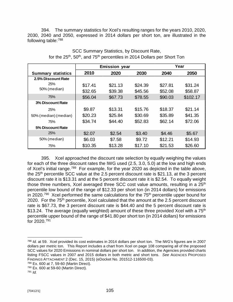
[70412/1] 105

394. The summary statistics for Xcel’s resulting ranges for the years 2010, 2020, 2030, 2040 and 2050, expressed in 2014 dollars per short ton, are illustrated in the following table:788

SCC Summary Statistics, by Discount Rate, for the 25th, 50th, and 75th percentiles in 2014 Dollars per Short Ton

Summary statistics Emission year Year

2010 2020 2030 2040 2050 2.5% Discount Rate

25% 50% (median)

$17.41 $32.65

$21.13 $39.38

$24.39 $45.56

$27.81 $52.08

$31.24 $58.87

75% $56.04 $67.73 $78.55 $90.03 $102.17 3% Discount Rate

$9.87

$13.31

$15.76

$18.37

$21.14 25% 50% (median) (median)

$20.23 $25.84 $30.69 $35.89 $41.35

75% $34.74 $44.40 $52.83 $62.14 $72.06 5% Discount Rate

25% $2.07 $2.54 $3.40 $4.46 $5.67 50% (median) $6.03 $7.58 $9.72 $12.21 $14.93

75% $10.35 $13.28 $17.10 $21.53 $26.60 395. Xcel approached the discount rate selection by equally weighing the values

for each of the three discount rates the IWG used (2.5, 3.0, 5.0) at the low and high ends of Xcel’s initial range.789 For example, for the year 2020 as depicted in the table above, the 25th percentile SCC value at the 2.5 percent discount rate is $21.13, at the 3 percent discount rate it is $13.31 and at the 5 percent discount rate it is $2.54. To equally weight those three numbers, Xcel averaged three SCC cost value amounts, resulting in a 25th percentile low bound of the range of $12.33 per short ton (in 2014 dollars) for emissions in 2020.790 Xcel performed the same calculations for the 75th percentile upper bound for 2020. For the 75th percentile, Xcel calculated that the amount at the 2.5 percent discount rate is $67.73, the 3 percent discount rate is $44.40 and the 5 percent discount rate is $13.24. The average (equally weighted) amount of these three provided Xcel with a 75th percentile upper bound of the range of $41.80 per short ton (in 2014 dollars) for emissions for 2020.791

788 Id. at 59. Xcel provided its cost estimates in 2014 dollars per short ton. The IWG’s figures are in 2007 dollars per metric ton. This Report includes a chart from Xcel on page 108 comparing all of the proposed SCC values for 2020 Emissions in nominal dollars per short ton. In addition, the Agencies provided charts listing FSCC values in 2007 and 2015 dollars in both metric and short tons. See AGENCIES PROPOSED FINDINGS ATTACHMENT 2 (Dec. 15, 2015) (eDocket No. 201512-116500-03). 789 Ex. 600 at 7, 59-60 (Martin Direct). 790 Ex. 600 at 59-60 (Martin Direct). 791 Id.

[70412/1] 106

396. Xcel chose to retain and weigh all three of the IWG’s discount rates equally as a way to remain neutral on the question of discount rate choice. In Xcel’s estimation, this approach can allow the Commission to avoid the difficult, and what Xcel views as the possibly unresolvable debates, concerning the correct discount rate for the SCC.792 Xcel pointed out that its approach would also permit an easy substitution of other discount rates, also equally weighted, should the IWG update its discount rates in the future.793

397. Xcel acknowledged that its choice to establish the boundaries of its range at the 25th and 75th percentiles of the FSCC cost range based on the IWG raw data contained certain policy judgments involving its balancing of risk tolerance and practicability.794

398. In choosing the 25th and 75th percentiles symmetrically around the median value to define the SCC range, Xcel noted that, although including the range of values from the 1st through the 99th percentile would more accurately reflect the full range of risks reflected in the IAM results, the full range would be impracticable because the resulting cost value range would extend from $-9 per ton to $600 per ton. Xcel asserted that such a broad range would not provide meaningful information to the Commission in the resource planning context.795 Xcel chose its 25th and 75th percentile cutoff points based on the relatively low probability of the lower and higher values occurring, in comparison with the values it targeted in its approach.796 Because it excluded low and high ends symmetrically, Xcel asserted that there was no bias in the way it limited its proposed SCC range.797

399. Xcel requested Brattle to calculate the probability that its initial 25th/75th percentile range (before the averaged discount rate amounts) contains the value of FSCC damages consistent with those predicted by the IWG’s IAMs.798 Given that each year of the FSCC distribution contains 150,000 values for a specific discount rate, when all three discount rates are included there are a total of 450,000 FSCC values per year. Brattle calculated that, for the Xcel distribution for 2020 from the 25th to the 75th percentile, the range included approximately 75 percent of the FSCC’s 450,000 data points.799 Xcel’s conclusion, based on Brattle’s calculation, is that there is a 75 percent chance that Xcel’s underlying statistics “capture the value of future climate change damages as predicted by the IAMs.”800 Xcel further reasoned that the IAMs climate change damages excluded from consideration below the 25th percentile and above the 75th percentile only represent a 25 percent chance of encompassing the cost of future climate change damages predicted by the IAMs.801

792 Id. at 60. 793 Id. 794 Id. at 60-61. 795 Id. 796 Id. at 61. 797 Id. 798 Id. at 62. 799 Id. at 62-63. 800 Ex. 600 at 63 (Martin Direct). 801 Id.

[70412/1] 107

400. After averaging the discount rate values at the 25th and 75th percentiles of the 2020 range (in 2014 dollars per short ton), Xcel’s proposed FSCC values for that year are $12.33 to $41.80. Brattle calculated that this range would correspond to the 36th and 74th percentiles of future climate change damages predicted by the IAMs for 2020.802 Thus, after averaging the discount rate values, 35 percent of the IAMs values are below Xcel’s range, while 26 percent are above the high end.803

401. Xcel maintained that that, when superimposed on the FSCC probability distribution curve, it is apparent that its proposed range excludes more of the higher-probability but lower-cost damages relative to the amount of lower-probability but higher-cost damages it includes.804 Xcel illustrated this in its Figure 9 of Mr. Martin’s testimony:805

802 Id. 803 Id. at 64. According to Mr. Martin, the low end of Xcel’s range, after averaging the discount values, is the 36th percentile, and 36 percent of the values predicted by the IAMS are below the low end of the proposed range. Id. at 63. The Administrative Law Judge assumes this is a misstatement on Mr. Martin’s part and he meant 35 percent of the values are below the low end. 804 Id. at 64. 805 Id. at 65.

[70412/1] 108

402. Xcel maintained that it made no other subjective judgments in its proposed SCC calculations because its method used results from the IWG IAMs, socioeconomic/emissions futures and discount rates. Xcel stressed that it did not prefer one of the IAMs or emissions models over another; and that it equally weighed the three discount rate values chosen by the IWG.806

403. Xcel’s final proposed ranges for each of the five years for which the IWG provided FSCC cost values, are as follows:807

CO2 Environmental Cost Values Proposed for Commission Adoption in 2014 Dollars per Short Ton

Proposed

Range 2010 2020 2030 2040 2050

Low $9.78 $12.33 $14.52 $16.88 $19.35 High $33.71 $41.80 $49.49 $57.90 $66.94

404. Xcel provided a comparison of the parties’ proposed CO2 values, for 2020 emissions, in nominal dollars per short ton:808

806 Ex. 600 at 61 (Martin Direct). 807 Id. at 62. Xcel also provided annual low and high values in 2014 dollars per short ton, and in nominal dollars per short ton. Ex. 600, NFM-1, Schedules 3, 4 (Martin Direct). 808 Ex. 601 at 12 (Martin Rebuttal). The Agencies provided additional comparative charts. See AGENCIES PROPOSED FINDINGS ATTACHMENT 2 (Dec. 15, 2015) (eDocket No. 201512-116500-03).

[70412/1] 109

VII. Criticisms of Xcel Proposal

A. The median versus the mean

405. The CEOs criticized Xcel’s use of the median rather than the mean to calculate the SCC. The CEOs asserted that the median is more appropriately used in a context where the goal is to understand a typical representation of the subject. In the case of future climate change, there is no typical future climate to consider.809 Instead, the CEOs argued that the mean incorporates information about the magnitude as well as the likelihood of damages, as reflected in the tails of the distribution. The CEOs asserted that the median only recognizes the magnitude of damages at the middle of the probability distribution and leaves out information about high damage outcomes, which the CEOs contend should be of greatest concern.810

406. The Agencies also disagreed with Xcel’s use of the median instead of the mean in developing the distribution of its SCC values.811 Noting that Xcel acknowledged that the FSCC values developed by the IWG are not normally distributed but instead are skewed with a long right tail, the Agencies disagreed with Xcel’s statement that the resulting skewed distribution results in a mean that is greatly influenced by “outliers.”812

407. According to the Agencies, “outlier” is defined in the field of statistics as “an observation that is distant from other observations.”813 The Agencies argued that the long right tail in the IWG distribution is a continuum of observations with increasingly large values, not outlier values disconnected from the rest of the observations on the continuum. The FSCC distribution is simply skewed, with a long right tail which includes some larger data points, said the Agencies.814

408. The CEOs provided an analogy between estimated CO2 damage cost calculations and home insurance pricing, stating that both processes involve uncertainty about what damages might occur in the future. The value of home insurance is above zero because there is some small chance that a damage-causing event, such as a severe storm or fire, will occur to the homeowner’s home within the next year. If there is a 5 percent chance such an event will occur, say the CEOs, there is a 95 percent chance that it will not. The CEOs stated that, in this scenario, if one calculates the median of expected damages over the coming year, the number is zero, including in the range from the 25th to the 75th percentile, regardless of how high the damages could be in the 5 percent likelihood that the home will be damaged. If the mean is used to understand the risk to the home, the CEOs argued, it provides a much clearer picture of the actual risk to the home by incorporating information about damages from the 5 percent chance of an event that will cause damage. The mean is the amount that will form the basis for the insurance

809 Ex. 101 at 37; Schedule 1 at 26 (Polasky Rebuttal). 810 Ex. 101 at 37 (Polasky Rebuttal); see also Ex. 801 at 68-69 (Hanemann Rebuttal). 811 Ex. 801 at 66 (Hanemann Rebuttal). 812 Id. at 66-67. 813 Id. at 67, fn 47. 814 Id. at 67.

[70412/1] 110

price. This, contended the CEOs, is the concept to use when calculating SCC damages.815

409. The Agencies also viewed the valuation of the social cost of carbon as a risk management process, the goal of which is “to avoid the risk of possibly very harmful climatic outcomes in the right tail of the warming and SCC probability distributions.” Because use of the median removes the tails of the distribution from consideration, the Agencies argued that approach is contrary to the goal of a risk management policy.816

410. In response to Xcel’s criticism that the FSCC was based on a single point rather than a range, the CEOs explained that the IWG took the mean across its 150,000 model runs for each of the three different discount rates it chose to calculate a mean-based value for each discount rate. According to the CEOs, these three rates provide three of the four points in the FSCC’s range of values. Thus the FSCC does provide a range and not only a single point.817

411. The CEOs pointed out that, although Xcel uses the median in establishing the range of percentiles to define its 25th and 75th percentiles, it uses the mean when it averages the three discount rate amounts.818

B. The range of values

412. The CEOs agreed with Xcel that having too much information (or too many points) within a range of values in the probability distribution for the SCC can make the range of values impractical for resource planners.819 However, the CEOs criticized the method Xcel used to create its range as arbitrary and resulting in a more subjective estimate of the SCC.820

413. The CEOs alleged that, because Xcel’s range only encompasses the 25th to the 75th percentile of the IWG outcomes, there is a 50 percent probability that the actual CO2 damages are outside the scope of Xcel’s SCC range.821 The CEOs contended that there is nothing unique about Xcel’s chosen endpoints and that a range extending from the 5th to the 95th percentile, for example, would encompass 90 percent of the IWG outcomes.822 The CEOs argued that Xcel’s range is less practical for use in resource planning decisions.823

414. The CEOs stated that Xcel’s range can lead to misleading representations of the FSCC. Using an example of the IWG process for the 3 percent discount rate (in 2007 dollars for 2020 emissions), the CEOs asserted that the range between the 25th and 815 Ex. 101 at 38-39 (Polasky Rebuttal). 816 Ex. 801 at 70 (Hanemann Rebuttal). 817 Ex. 101 at 39 (Polasky Rebuttal). 818 Id. 819 Id. at 40. 820 Id. 821 Id. at 41. 822 Id. 823 Id. at 40-41.

[70412/1] 111

75th percentiles is $13 to $44, and that the mean value is $43, just one dollar lower than the 75th percentile value.824 Because the CO2 damage distribution is a skewed distribution, the CEOs stated that the mean value of the damages may lie outside the 25th to 75th percentile range.825 On the other hand, the CEOs argued, using the 5th and 95th percentiles creates a dollar value range from $2 to $128, which is only $11 lower than the low end, but $84 higher than the upper end of Xcel’s range. The larger range better captures the uncertainty in the SCC, according to the CEOs.826

415. The CEOs supported the IWG’s approach, which is to use the mean in the range of values at a given discount rate, because the mean “incorporates all the values of the distribution and is not arbitrarily chosen.”827 The CEOs viewed the IWG’s approach as a way to capture the broad distribution of values while still offering the Commission a practical number of values from which to choose.828

C. Averaging the discount rates

416. The CEOs also criticized Xcel’s decision to average the values of the three discount rates for each end of its distribution range, stating that “[t]here is no reasonable argument that the mean value across the three discount rates is an appropriate measure of the SCC.”829

417. In addition, the CEOs stated that Xcel’s averaging of values of the discount rates is not supported by any theoretical basis because the SCC calculation does not involve considering the entire range of discount rates, or applying a probability distribution to the likelihood of a particular rate being the “ ‘true’ social discount rate.”830

418. The CEOs stressed that only a moderator or regulator can choose the appropriate discount rate. The CEOs objected to Xcel’s approach, which makes it impossible to consider any one of the rates individually. The CEOs supported the IWG’s approach, which maintained separate values for each of the three discount rates it considered theoretically appropriate, leaving policy-makers free to apply the most suitable rate in the circumstances.831

419. Peabody rejected Xcel’s proposal to weight the various discount rates equally as a way to solve the problem of the Commission having to confront the discussion of which discount rate is most appropriate, because “[i]gnoring the problem and using flawed data do not provide an acceptable solution to the problem.”832

824 Ex. 101 at 41 (Polasky Rebuttal). 825 Id. 826 Id. 827 Id. 828 Id. at 41-42. 829 Id. at 42-43. 830 Id. at 43. 831 Id. 832 Ex. 233 at 50 (Bezdek Rebuttal Ex. 1).

[70412/1] 112

D. Exclusion of 95th Percentile of FSCC Distribution

420. The Agencies also disagreed with Xcel’s decision to exclude the IWG’s 95th percentile of the FSCC distribution from consideration in Xcel’s distribution.833 The Agencies pointed out that, in other regulatory contexts, a 5 percent risk with potentially catastrophic outcomes is considered. In support of the importance of recognizing the 95th percentile, the Agencies quoted a report on the value at risk from climate change by the Economic Intelligence Unit, pointing out that people “wouldn’t get on a plane if there was a 5% chance of the plane crashing, but we’re treating the climate with that same level of risk in a very offhand, complacent way.”834

421. The Agencies asserted that the concern with risks associated with the tails of the distribution range is consistent with, and validates, the decision to report the 95th percentile value of the FSCC distribution.835

E. Xcel’s Criteria for Reviewing the FSCC

422. The Utilities and MLIG criticized Xcel’s eight proposed criteria for reviewing potential environmental cost values. The Utilities and MLIG maintained it is important for the Commission to have specific review criteria. The Utilities and MLIG supported the notion of the Commission adopting the criteria it used in the first Externalities docket,836 and criticized Xcel because its criteria are “fundamentally different criteria from those previously relied upon by the Commission.”837 Specifically, the Utilities and MLIG rejected Xcel’s proposed criterion advising that the SCC “[r]eflect an appropriate level of risk tolerance, i.e. tolerance for risk that the actual value of future climate change damages may lie outside the Commission’s adopted range . . . .”838

423. The Utilities and MLIG asserted that this criterion calls for “speculative subjectivity,” making it inconsistent with another of Xcel’s criteria, which calls for minimizing subjective judgments.839

833 Ex. 801 at 70 (Hanemann Rebuttal). 834 Id. 835 Id. at 71. 836 The Utilities and MLIG did not specify whether they were referring to the criteria set out in Judge Klein’s Recommended Order or to the criteria listed in the Commission’s Order. Because the “conservative value” criterion was not explicitly adopted by the Commission, the Administrative Law Judge presumes the Utilities and MLIG were referring to Judge Klein’s Recommended Order. Compare Ex. 305, In the Matter of the Quantification of Envtl Costs Pursuant to Laws of Minn. 1993, Chap. 356, Sec. 3, PUC Docket No. E-999/CI-93-583, FINDINGS OF FACT, CONCLUSIONS, RECOMMENDATION AND MEMORANDUM at 17 (March 22, 1996), with 93-583 PUC ORDER 1 at 11-14. 837 Ex. 304 at 6-7 (Smith Surrebuttal). 838 Id. 839 Id.

[70412/1] 113

F. Use of the Underlying FSCC Data

424. Peabody criticized Xcel generally for accepting the IWG’s numbers as a basis for Xcel’s SCC proposal. Given all of the perceived flaws in the IWG process and the fundamental disagreement that Peabody had with the IWG’s underlying assumptions, Peabody found that Xcel’s proposed values were also meaningless.840 In particular, Peabody asserted that Xcel should have included the 7 percent discount rate in its proposed SCC model.841

425. Peabody accused Xcel of misusing statistics and probability theory in its proposal to capture 75 percent of the IAMs’ data. Peabody’s criticism in this regard focused on its rejection of the underlying IWG data.842

426. Peabody also rejected the idea that the FSCC, and therefore Xcel’s proposed SCC, minimizes subjective judgments.843

G. Xcel’s Responses to Criticisms of Its Proposal

427. In response to criticism of the Xcel model’s use of the median versus the mean, Xcel claimed it did not propose adopting a median instead of a mean.844 Xcel argued a median “would be a single point estimate,” which it did not recommend.845 Rather, the Company proposed using “the 25th percentile at 5 percent discount rate and the 75th percentile at 2.5 percent discount rate as the low and high bounds of its initial range, and then equally weighted the values at each discount rate at each end of the range.”846 Xcel believed the proposed percentiles “strike an appropriate balance of accounting for uncertainty, risk tolerance, and practicability.”847

428. Xcel reiterated its criticisms of the use of the mean because of the “non-normal, right-skewed shape” of the FSCC probability distribution. Xcel argued that the mean in this situation is not trustworthy because IAMs did not completely capture damages at either the high or low end, and it is difficult to know where the errors are greater.848

429. Xcel continued to advocate for a range of values, maintaining that a range provides more, rather than less, information for resource planning purposes and will ensure that resource plans will be “robust” under various assumptions.849

840 Ex. 233 at 44-49 (Bezdek Rebuttal Ex. 1). 841 Id. at 46. 842 Id. at 50-51. 843 Id. at 51-52. 844 Ex. 602 at 9 (Martin Surrebuttal). 845 Id. 846 Id. 847 Id. at 11. 848 Id. 849 Id. at 38.

[70412/1] 114

430. Xcel responded to the CEOs’ criticism that Xcel used the mean when averaging discount rates, but not when choosing values in the FSCC distribution range. Xcel asserted that equally weighting the FSCC values at different discount rates is qualitatively different from finding the mean value for purposes of determining the SCC, and it has a different justification.850 Xcel explained that it equally weighted the discount rates in an effort to remain neutral regarding an issue where there is no consensus and that “raises highly contested and exceedingly difficult questions of science, economics, philosophy, and law.”851

431. In response to criticism of the Xcel model’s exclusion of the 95th percentile, Xcel argued that “adopting the 95th percentile would have to be accompanied by adopting the 5th percentile,” which would not be practical because the two percentiles “point in opposite directions.”852 Xcel believed risk tolerance must “be bounded in good public policymaking,” and therefore asserted “it is inappropriate for the Commission to intentionally set the SCC at a level that is by definition 95 percent likely of being too high.”853

432. In response to criticism that the Xcel model should not accept the IWG’s raw numbers as a basis for its model, Xcel argued that deriving new numbers to base the model on “would have required the Company to make myriad scientific and subjective policy judgments.”854 Instead, Xcel used the IWG modeling outputs as a starting point and worked to “find a way to make them more practicable and appropriate for integrated resource planning in Minnesota.”855 According to Xcel, the “IWG’s modeling outputs are far from perfect, but no other witnesses have proposed a clearly superior damage cost approach that does not involve subjective judgments of their own and/or require laborious new modeling each time the Commission updated its CO2 environmental cost range.”856

433. In response to criticism that the Xcel model accepts the IWG’s subjective policy judgments as a basis for the model, Xcel conceded that it “lacks expertise to substitute its judgment for that of the IWG and the climate scientists and economists” in selecting the “analytical framing assumptions” necessary for the model.857

CONCLUSIONS

1. The Public Utilities Commission and the Administrative Law Judge have jurisdiction to consider this matter pursuant to Minn. Stat. §§ 14.50, 216B.01-.82 (2014), and Minn. R. 7829.1000 (2015).

850 Ex. 602 at 37 (Martin Surrebuttal). 851 Id. 852 Id. at 16. 853 Id. at 17. 854 Id. at 5. 855 Id. 856 Id. 857 Id. at 6.

[70412/1] 115

2. The public and the parties received proper and timely notice of the hearings and the Commission and all parties complied with all procedural requirements of statute and rule.

3. The Administrative Law Judge concludes that the following burdens of proof apply in this proceeding:

a. A party or parties proposing that the Commission adopt a new environmental cost value for CO2, including the Federal Social Cost of Carbon, bears the burden of showing by a preponderance of the evidence that the value being proposed is reasonable and the best available measure of the environmental cost of CO2.

b. A party or parties proposing that the Commission retain any environmental cost value as currently assigned by the Commission bears the burden of showing by a preponderance of the evidence that the current value is reasonable and the best available measure to determine the applicable environmental cost.

c. A party or parties opposing a proposed environmental cost value must demonstrate that the evidence offered in support of the proposed values is insufficient to amount to a preponderance of the evidence.

I. Use of IAMS as Damage Cost Models

4. The Administrative Law Judge concludes that the Commission’s Notice and Order for Hearing in this docket require the parties to evaluate the environmental cost values using a damage cost, as opposed to market-based or cost-of-control approach. The Commission found the damage-cost approach superior to a market-based or cost-of-control approach “because it appropriately focuses on actual damages from uncontrolled emissions.”858

5. The Administrative Law Judge concludes that taking the cost of emissions abatement into account when calculating damages is contrary to the Commission’s understanding of a damage-cost approach, which focuses “on actual damages from uncontrolled emissions.”859

6. The Administrative Law Judge concludes that the Agencies and the CEOs demonstrated, by a preponderance of the evidence, that the IWG’s use of the DICE, PAGE, and FUND models to calculate the FSCC is a damage-cost approach consistent with the Commission’s Notice and Order for Hearing in this docket.860

858 NOTICE AND ORDER FOR HEARING at 4 (Oct. 15, 2014) (eDocket No. 201410-103872-02). 859 Id. 860 Id.

[70412/1] 116

7. The Administrative Law Judge concludes that the Commission required any consultant retained by the Agencies to use reduced-form modeling to estimate damage costs in this proceeding.861

8. The Administrative Law Judge concludes that the Agencies and the CEOs demonstrated, by a preponderance of the evidence, that it was reasonable for them to rely on an environmental cost valuation for CO2 based on the use of the DICE, PAGE and FUND models, given the combined requirements of a damage-cost approach and reduced-form modeling.

9. The Administrative Law Judge concludes that the Agencies and the CEOs demonstrated, by a preponderance of the evidence, that the IAMs’ damage functions were based on empirical studies. However, the Administrative Law Judge further concludes that the empirical evidence on which the IWG relied to calculate damage functions for the FSCC consisted of fewer than fifty empirical studies, which were neither up-to-date nor comprehensive, adding to the uncertainty of the FSCC estimates, particularly in the areas of catastrophic damages and the treatment of the distant future.

10. The Administrative Law Judge concludes that more studies, using new approaches, have been published since the last update of the FSCC and that the IWG has expressed a commitment to continuing to pursue the most current research and to incorporate it as appropriate into future FSCC updates. The Administrative Law Judge concludes that, if the Commission adopted the FSCC, the Commission could update its CO2 environmental cost values in the future as the IWG revised the FSCC based on more current research.

11. The Administrative Law Judge concludes that a preponderance of the evidence demonstrates that the FSCC underestimates the negative effects that increased warming will have on human health.

12. The Administrative Law Judge concludes that a preponderance of the evidence demonstrates that the IAMs damage functions do not account for a significant number of important environmental impacts which will occur as a result of climate change.

13. The Administrative Law Judge concludes that, based on unreported and underreported health and environmental impacts, along with the IWG’s acknowledgement that the FSCC is not based on the most current research, the preponderance of the evidence demonstrates that the FSCC understates the full environmental cost of CO2.

II. IWG’s Choice and Application of Discount Rates

14. The Administrative Law Judge concludes that the preponderance of the evidence demonstrates that both the three percent discount rate and the five percent discount rate are recognized as consumption rates of discount and it is reasonable to apply the three- and five- percent discount rates to the SCC.

861 Id. at 5.

[70412/1] 117

15. The Administrative Law Judge concludes that Peabody, and the Utilities and MLIG failed to demonstrate by a preponderance of the evidence that a Ramsey rule discount rate that adjusts over time is reasonable to use in calculating the SCC. That approach is not appropriate because it is based on the concept that climate policy can be viewed through the metaphor of a single, infinitely-lived individual rather than the changing views of societies as they evolve over generations. The Administrative Law Judge concludes that the Ramsey rule fails to take into account the idea that priorities and preferences of people and societies will change over an extended period of time and does not address issues of equity between generations. Furthermore, the Administrative Law Judge concludes the Ramsey rule is not appropriate in this proceeding because it begins with a higher discount rate which declines with time. In addition to the intergenerational nature of the FSCC damage calculation, due to the uncertainties associated with the possibility of catastrophic damages from a “tipping point” event which may occur at an unknown time, and the understatement of impacts in the IAMs’ damage functions, the Administrative Law Judge concludes that an approach that is designed to begin with a higher discount rate and gradually declines is neither reasonable nor the best approach to for the purpose of calculating an SCC.

16. The Administrative Law Judge concludes that the preponderance of the evidence demonstrated that the OMB Circular A-4 does not require the IWG to use the seven percent discount rate to calculate the FSCC, because the Circular A-4 is advisory and not mandatory in nature. The Administrative Law Judge concludes that the OMB participated in the IWG’s development of the FSCC and there was no evidence that the OMB objected to the IWG’s choice not to use a seven percent discount rate in calculating the FSCC.

17. The Administrative Law Judge concludes that the proposal advanced by the Utilities and MLIG to increase the upper end of the discount rate range to incorporate the opportunity cost of emissions reductions in the IWG’s IAMs would be a “cost-of-control” approach, contrary to the Commission’s required damage-cost approach.

18. The Administrative Law Judge concludes that the Agencies and the CEOs demonstrated, by a preponderance of the evidence, that the IWG’s choice of a 2.5 percent rate of discount is within the existing bounds of rates used in other climate change models. The 2.5 percent rate of discount is a reasonable approach to account for the multi-generational scope of the FSCC and to address the concern that interest rates are uncertain over time.

19. The Administrative Law Judge concludes that Peabody failed to demonstrate, by a preponderance of the evidence, that the IWG’s discount rates are arbitrary.

III. 95th Percentile Value at 3 Percent Discount Rate

20. The Administrative Law Judge concludes that the CEOs and the Agencies demonstrated by a preponderance of the evidence that the FSCC likely understates

[70412/1] 118

damages and that the risk of a “tipping point” is not well-represented within the scope of the 2.5, 3.0 and 5.0 percent rate of discount.

21. Nonetheless, the Administrative Law Judge concludes that the CEOs and the Agencies failed to demonstrate, by a preponderance of the evidence, that the 95th percentile value at a three percent discount is a reasonable means of representing the high side of the FSCC distribution. The Agencies and the CEOs failed to demonstrate a reasonable basis for choosing the 95th percentile at three percent to represent the uncertainties regarding understated damages and a potential “tipping point.” The 95th percentile value provided a larger damages number but was not supported by specific evidence or reasoning to demonstrate that the number is a meaningful estimate of the uncertainties it represents.

IV. Equilibrium Climate Sensitivity

22. The Administrative Law Judge concludes that Peabody failed to demonstrate, by a preponderance of the evidence, that an ECS value of 1 or 1.5 degrees centigrade is correct and that an ECS of more than 2 degrees centigrade is “extremely unlikely.”

23. The Administrative Law Judge concludes that the preponderance of the evidence demonstrates that the ECS doubling ranges as reported by the IPCC in the IPCC AR4 (2.0-4.5 °C) and the IPCC AR5 (1.5-4.5 °C) are more accurate ECS ranges than the range advanced by Peabody because the IPCC ranges are representative of a comprehensive, peer-reviewed body of scientific study based on multiple lines of evidence.

24. The Administrative Law Judge concludes that the preponderance of the evidence demonstrates the IWG had a reasoned basis to refrain from adopting the IPCC AR5 ECS values in the IWG’s 2013 FSCC update. While the IWG could have chosen to adopt the updated values at that time, it stated that it viewed that IPCC AR4 ECS values as the most authoritative at the time of the 2013 update and affirmed its intention to update the ECS values as appropriate in the future, based on the latest science and external expert advice.

25. The Administrative Law Judge concludes that the preponderance of the evidence demonstrates that it was reasonable for the IWG to adopt the ECS range of 2.0-4.5 °C as stated in the IPCC AR4.

V. Marginal Ton

26. The Administrative Law Judge concludes that the Utilities and MLIG failed to demonstrate, by a preponderance of the evidence, that the proposal to value CO2 emissions by using baselines in which there are no additional emissions of CO2 after the incremental emission is a reasonable approach to measuring damages in this proceeding. The Utilities and MLIG based this approach on the idea that incremental emissions reduction costs should be balanced with societal damage costs in calculating the SCC. This approach is contrary to the Commission’s understanding of a damage-cost approach

[70412/1] 119

because, by incorporating the cost of emissions reductions, the Utilities’ and MLIG’s proposal incorporates a “cost-of-control” approach.

27. The Administrative Law Judge concludes that the Utilities and MLIG failed to demonstrate, by a preponderance of the evidence, that the proposal to value CO2 emissions by using baselines in which there are no additional emissions of CO2 after the incremental emission is a reasonable approach because this approach presumes an effective global emissions reduction program will be in effect. The Utilities and MLIG failed to present any evidence of such a program.

28. The Administrative Law Judge concludes that the Utilities and MLIG failed to demonstrate by a preponderance of the evidence that the proposal to value CO2 emissions by using an average ton approach is a reasonable approach in this proceeding. The Administrative Law Judge concludes that by averaging the first and last tons to calculate the average ton, the Utilities’ and MLIG’s average ton incorporates the cost of emissions reductions. Therefore, the Utilities’ and MLIG’s proposal incorporates a “cost-of-control” approach. In addition, the Administrative Law Judge concludes that the Utilities and MLIG failed to demonstrate that the Commission used an average ton approach in the first Externalities case.

29. The Administrative Law Judge concludes that the Agencies and the CEOs demonstrated, by a preponderance of the evidence that the FSCC’s approach to counting the last ton of CO2 emitted as the marginal ton is reasonable and the best approach to calculate damages. This is the best and most reasonable approach because it most closely matches the scientific understanding of what is known about the nature of CO2, which is that each ton of CO2 emitted has a cumulative impact, both with respect to the CO2 emitted in the past and the CO2 emitted in the future, as long as that ton of CO2 remains in the atmosphere.

VI. Modeling Time Horizon

30. The Administrative Law Judge concludes that a preponderance of the evidence demonstrates that a ton of CO2 released into the atmosphere will not be fully absorbed into the land or the oceans for a minimum of two hundred years. The Administrative Law Judge finds that it will be hundreds of years before that ton will be fully absorbed.

31. The Administrative Law Judge concludes that a preponderance of the evidence demonstrates that CO2 will continue to have a cumulative impact on the climate for as long as it remains in the atmosphere.

32. The Administrative Law Judge concludes that the CEOs and Agencies failed to demonstrate that the IWG’s prediction of damages from the year 2100 to the year 2300 meet the same standards of reliability as the IWG’s predictions of damages from the present to the year 2100. The IWG used the peer-reviewed EMF-22 emissions scenarios, which were constructed through the year 2100. The IWG extrapolated the EMF inputs to the year 2300 based on limited data, without the benefit of peer review.

[70412/1] 120

33. The Administrative Law Judge concludes the Utilities and MLIG demonstrated by a preponderance of the evidence that approximately 50 percent of the FSCC estimates at a three percent rate are in the post-2100 era.

34. The Administrative Law Judge concludes that the Agencies and the CEOs failed to demonstrate by a preponderance of the evidence that a modeling time horizon extending to the year 2300 is reasonable. An additional two-hundred years will add increased numbers of cost values at lower interest rates and accelerating rates of damages with the passage of time and increased temperature. Therefore, the Administrative Law Judge finds that an extrapolation extending two-hundred years beyond the year that the EMF-22 scenarios were constructed to end is a degree of uncertainty that is not reasonably supported by adequate evidence.

35. However, weighing the importance of accounting for the CO2 that will remain in the atmosphere beyond the year 2100, and the understated nature of the FSCC, the Administrative Law Judge concludes that it is reasonable to implement the IWG’s extrapolation for 100 years, to the year 2200. While the evidentiary underpinning is no greater for this extrapolation than it would be to extend the model to the year 2300, this approach lessens the danger of multiplication of errors within the extrapolation while providing a response to the strong evidence of damage from CO2.

VII. Geographic Scope

36. The Administrative Law Judge concludes that the preponderance of the evidence in this docket demonstrates that CO2 emissions emitted in one location on the Earth mix with GHGs emitted from all other locations on the planet, with each GHG molecule contributing to climate change experienced everywhere. In addition, in the first Externalities proceeding the Minnesota Court of Appeals held that, “[r]egardless of its emission point, CO2 is believed to contribute to global warming, which in turn adversely impacts the global environment.”862

37. The Administrative Law Judge concludes that the Utilities and MLIG failed to demonstrate, by a preponderance of the evidence, that limiting damages to the United States or Minnesota will capture all of the damage caused by CO2 emissions released from electric power generating facilities within Minnesota.

38. The Administrative Law Judge concludes that MLIG improperly framed the calculation of the environmental cost value of CO2 as a question of economic standing by stating the question in terms of who pays the costs of the policy and who receives the benefits.

39. The Administrative Law Judge concludes that Minn. Stat. § 216B.2442, subd. 3, and the Commission’s requirement that the parties use a damage-cost analysis compel that the question of the geographic scope of damages be viewed in terms of the source of the CO2 emissions and all their damaging impacts, wherever they are 862 In re Quantification of Envtl Costs, 578 N.W.2d 794, 796 (Minn. Ct. App. 1998), review denied (Minn. Aug. 18, 1998).

[70412/1] 121

experienced. Therefore, the Administrative Law Judge concludes that this proceeding requires a global scope for damages.

VIII. Leakage

40. The Administrative Law Judge concludes that the preponderance of the evidence demonstrates that calculating leakage of increased CO2 emissions is not properly a part of this proceeding.

IX. Uncertainty

41. The Administrative Law Judge concludes that the preponderance of the evidence shows that the task of predicting the SCC is highly uncertain, because it is an exercise in predicting impacts of CO2 emissions many years into the future. The process involves forecasting such uncertainties as changing temperatures, global GDP far into the future, and the possible occurrence of a “tipping point” event leading to irreversible, catastrophic damages.

42. The Administrative Law Judge concludes that the preponderance of the evidence demonstrates the IWG partially accounts for uncertainty in the FSCC by using three IAMs, five different socioeconomic emissions projections and probability distributions for the ECS values, as well as a number of parameters in the FUND and PAGE IAMs.

43. The Administrative Law Judge concludes that the Agencies and CEOs demonstrated by a preponderance of the evidence that, given the increased scientific certainty of the link between CO2 emissions and climate change, uncertainties such as the potential danger of a “tipping point” catastrophe reasonably require an initially high SCC until more is known about such uncertainties.

X. Adaptation and Mitigation

44. The Administrative Law Judge concludes that the Agencies and CEOs demonstrated by a preponderance of the evidence that the IWG adequately accounted for adaptation and mitigation in the FSCC. No other party demonstrated by a preponderance of the evidence that it is reasonable to account for adaptation or mitigation to any extent beyond that included in the FSCC. There was no specific evidence presented regarding the efficacy of any specific mode of adaptation or mitigation.

45. The Administrative Law Judge concludes that approaching the damage calculation to achieve an “optimal mitigation level” such as Peabody recommended is not consistent with the cost-damage approach required by the Commission.

XI. Use of FSCC Outside of Federal Regulatory Setting

46. The Administrative Law Judge concludes that the preponderance of the evidence demonstrates that the IWG has not taken a position regarding whether it is appropriate for a state to adopt the FSCC for purposes such as those outlined in Minn.

[70412/1] 122

Stat. § 216B.2422, subd. 3. The Administrative Law Judge concludes that the FSCC could provide the Commission with the information it requires to implement Minn. Stat. § 216B.2422, subd.3. There was no evidence offered in this proceeding to demonstrate that the IWG’s FSCC values are different than they would have been had the IWG developed an SCC specifically for the purpose of complying with Minn. Stat. § 216B.2422, subd.3.

XII. Scientific Process

47. The Administrative Law Judge concludes that Peabody failed to demonstrate by a preponderance of the evidence that the IWG is neither peer-reviewed nor transparent. While the FSCC itself is not peer-reviewed, a preponderance of the evidence demonstrated that the IWG relied primarily on peer-reviewed literature, particularly the work of the IPCC, which is recognized by the Commission, the Minnesota Court of Appeals and the United States Supreme Court as a credible source of expertise in the area of climate change. The experts in this proceeding reviewed the FSCC process exhaustively, providing extensive analysis and critique. While technically not a peer review, this contested case process has provided a thorough level of scrutiny of the FSCC and the IWG’s process in developing the FSCC. The IWG’s Technical Support Documents are all part of the record in this proceeding, along with numerous commentaries regarding the IWG’s process and the FSCC.

48. The Administrative Law Judge concludes that Peabody failed to demonstrate by a preponderance of the evidence that the Agencies and the CEOs relied primarily on non-peer-reviewed literature. The Administrative Law Judge was unable to verify Peabody’s non-specific assertions that the Agencies and CEOs relied on such literature.

XIII. Xcel Proposal

49. The Administrative Law Judge concludes that Xcel failed to demonstrate by a preponderance of the evidence that its proposal to calculate the upper and lower SCC values at the 25th and 75th percentiles of the IWG data distribution was reasonable. The Administrative Law Judge concludes that, by choosing the 25th and 75th percentiles, Xcel centered its SCC range around the 50th percentile, which is the median of the distribution. By choosing to center its range around the median value, Xcel unreasonably excluded information about the magnitude, as well as the likelihood of significant damages, as reflected in the higher end tails of the distribution. These high damage outcomes are of great concern and it would be unreasonable to ignore them.

50. The Administrative Law Judge concludes that Xcel failed to demonstrate by a preponderance of the evidence that it had a reasonable basis on which to average the three FSCC discount rate values at the upper and lower ends of its range of values to establish its final SCC range of cost values. Xcel presented no evidence of theoretical, practical or scholarly support for its idea that averaging the values of the three discount rates for each end of its distribution range is an appropriate way in which to account for the controversy among the parties regarding a proper discount rate in this proceeding.

[70412/1] 123

51. The Administrative Law Judge concludes that Xcel failed to demonstrate by a preponderance of the evidence that the FSCC does not offer a range of values. The FSCC chooses one cost based on an average of the values on the distribution scale, then creates a range of values from the single cost by offering that value at three different discount rates, and adding the 95th percentile as a fourth high-end value.

XIV. Reasonable and the Best Available Measure of CO2

52. The Administrative Law Judge concludes that Peabody failed to demonstrate by a preponderance of the evidence that any of the CO2 environmental cost values it proposed are reasonable and the best available measure of CO2 cost values.

53. The Administrative Law Judge concludes that MLIG failed to demonstrate, by a preponderance of the evidence, that any of the CO2 environmental cost values it proposed are reasonable and the best available measure of CO2 cost values.

54. The Administrative Law Judge concludes that the Utilities and MLIG failed to demonstrate, by a preponderance of the evidence, that any of the CO2 environmental cost values they proposed are reasonable and the best available measure of CO2 cost values.

55. The Administrative Law Judge concludes that Xcel failed to demonstrate by a preponderance of the evidence that its proposal for measuring CO2 cost values is reasonable and the best available measure of CO2 cost values.

56. The Administrative Law Judge concludes that the Agencies and the CEOs demonstrated by a preponderance of the evidence that the Federal Social Cost of Carbon is reasonable and the best available measure to determine the environmental cost of CO2, with the exceptions described in these findings regarding the 95th percentile and the time modeling horizon.

57. Any Findings of Fact more properly designated as Conclusions of Law are

hereby adopted as such.

Based upon these Conclusions of Law, the Administrative Law Judge makes the following:

RECOMMENDATIONS

1. The Administrative Law Judge respectfully recommends that the Commission adopt the Federal Social Cost of Carbon as reasonable and the best available measure to determine the environmental cost of CO2, establishing a range of values including the 2.5 percent, 3.0 percent, and 5 percent discount rates, with the following amendments:

[70412/1] 124

a. The FSCC values will be re-calculated to reflect a shortened time horizon extending to the year 2200.

b. The Commission will exclude the value derived from the 95th percentile at a 3 percent discount rate value from the range of values.

2. The Administrative Law Judge respectfully recommends that the Commission open an investigation into the questions of how to best measure leakage, and whether and how to take leakage into account in other proceedings, as suggested by Xcel in this proceeding.

Dated: April 15, 2016 _________________________________ LAURASUE SCHLATTER Administrative Law Judge Recorded: Digitally Recorded

NOTICE

Notice is hereby given that exceptions to this Report, if any, by any party adversely affected must be filed under the time frames established in the Commission’s rules of practice and procedure, Minn. R. 7829.2700, .3100 (2015), unless otherwise directed by the Commission. Exceptions should be specific and stated and numbered separately. The Commission will make the final determination of the matter after the expiration of the period for filing exceptions, or after oral argument, if an oral argument is held.

The Commission may, at its own discretion, accept, modify, or reject the

Administrative Law Judge’s recommendations. The recommendations of the Administrative Law Judge have no legal effect unless expressly adopted by the Commission as its final order.

[70412/1] 125

MEMORANDUM

The parties in this proceeding were very well-represented, offering their arguments thoroughly and vigorously. The record is large, in part because the parties raised so many issues in the discussion of how best to measure the social cost of carbon. The discussion was informative and wide-ranging. The Administrative Law Judge appreciates the parties’ significant efforts at insuring that the record in this proceeding is comprehensive.

I. Guiding Criteria

In reviewing the issues raised by the parties, the Administrative Law Judge has been guided by several criteria. The Commission established certain of these criteria in the first Externalities case.

In the first Externalities case, the Commission considered the statutory requirement that its task under Minn. Stat. § 216B.2422, subd. 3, is “to the extent practicable, [to] quantify and establish a range of environmental costs associated with each method of electricity generation.”863 In its January 1997 Order, the Commission adopted the Administrative Law Judge’s definition of the term “practicable” for purposes of the statute, finding that “practicable” means “feasible” or “capable of being accomplished.”864 Practicability must be demonstrated by a preponderance of the evidence, as discussed earlier in this report.865

The Commission established several additional criteria in 1997, several of which are relevant to this portion of the present docket.866 Those criteria are that: 1) the damage-cost approach is preferred; 2) using a range of environmental cost values appropriately takes into consideration a certain level of unavoidable scientific uncertainty; and 3) while it is generally appropriate to focus on damages occurring in Minnesota, that approach does not apply to values adopted for CO2, for which damages should be assessed globally.867 In addition, the Commission’s Notice and Order for Hearing in this docket required any consultant retained by the Agencies to use reduced-form modeling to estimate damage costs.868

II. Adopting Conservative Values

Several of the guiding criteria the Commission established in 1997 were first recommended by the Administrative Law Judge Allan Klein in his report as criteria “appropriate for use in determining which environmental impacts to value and whether

863 Minn. Stat. § 216B.2422, subd.3. 864 93-583 PUC ORDER 1 at 11. 865 93-583 PUC ORDER 1 at 13-14; ORDER REGARDING BURDENS OF PROOF at 2-3 (Mar. 27, 2015) (eDocket 20153-108636-01). 866 Certain principles in 93-583 PUC ORDER 1 are relevant to the Criteria Pollutants portion of the docket, but not to the CO2 portion. They are not discussed here. 867 93-583 PUC ORDER 1 at 13-16. 868 NOTICE AND ORDER FOR HEARING at 5 (Oct. 15, 2014) (eDocket No. 201410-103872-02).

[70412/1] 126

and how to value these impacts . . . .”869 However, the Commission did not adopt all of those principles in its 1997 Orders.

One of the criteria recommended by the Judge Klein but not mentioned in the Commission’s 1997 Orders was “[t]he adopted values should be conservative.”870 Judge Klein urged the Commission to adopt lower values,871

because . . . the quantification of environmental costs is still in its infancy. [Internal citation omitted.] While using reasonably accurate estimates is better than imputing no values, not all estimates are better than zero. For instance, valuing an impact at more than twice its “true” residual damage may lead to a worse allocation of resources than imputing no value. In other words, the possibility of utilities paying more for resources than their environmental benefits justify is just as bad as paying less than their benefits justify. Given the current uncertainty regarding the estimation process, overestimating the damages is a distinct possibility.

In this docket, the Utilities, MLIG and Peabody each cited Judge Klein’s language regarding conservative values, along with the cost values the Commission adopted in that docket, to support their arguments that the Commission should adopt conservative cost values in this proceeding.872 Contrary to the arguments made by Peabody, MLIG and the Utilities, there is no explicit language in the Commission’s 1997 Order approving Judge Klein’s reasoning regarding adopting conservative cost values. The values chosen by the Commission in 1997 were based on the lower of two ranges recommended by the Minnesota Pollution Control Agency (MPCA). The Commission’s reasoning for choosing the lower range was based on its determination that the lower range was better supported by the evidence in the record. The Commission made no mention of Judge Klein’s “conservative cost value” approach.873

Even if the Commission understands the 1997 Order to be based on an implicit adoption of Judge Klein’s “conservative cost value” approach, this Administrative Law Judge respectfully recommends that the Commission not follow that approach in this proceeding. Judge Klein did not explain the reasoning underlying his statement that “the possibility of utilities paying more for resources than their environmental benefits justify is just as bad as paying less than their benefits justify.”874 Judge Klein did not say why the Commission should have been more concerned about risking an error that would cost more money than absolutely necessary to avoid environmental damage than an error that would cost more damage because too little money was spent. Perhaps, in 1997, the

869 Ex. 305 at 12 (1996 Report). 870 Id. 871 Id. at 17. 872 See, e.g., MLIG’s Initial Br. at 11, 22 (November 24 2015); Peabody’s Initial Br. at 1, 11, 15, 17, 31 (November 24 2015); Utilities’ Initial Br. at 7 (November 24 2015). 873 93-583 PUC ORDER 1 at 25-26. 874 Ex. 305 at 17 (1996 Report).

[70412/1] 127

science was less clear than it was by 2015 about the consequences of allowing climate change to continue.

While estimating damages, particularly far into the future, remains a difficult problem full of uncertainty, there is now undeniable evidence that CO2 emissions are already having a dramatic impact on the Earth and its climate. A modern proverb graphically illustrates the dichotomy of conservatism in the face of climate change: “When the last tree is cut down, the last fish eaten, and the last stream poisoned, you will realize that you cannot eat money.”875 In establishing cost values in this proceeding, the Administrative Law Judge respectfully recommends that the Commission consider applying conservative values to the well-being of future generations and the planet needed to sustain them, rather than primarily to the financial cost of providing that well-being.876

III. DHE and CEBC Testimony

As noted in footnote 162, supra, MLIG argued in its post-hearing brief in this proceeding that neither DHE nor CEBC introduced “admissible foundational evidence to support adoption of the FSCC.”877

IV. DHE Testimony

As to DHE, MLIG argues that DHE’s witness, Dr. Rom, while well-qualified as a physician, is not qualified to provide an opinion as to “the reliability, practicability, or appropriateness of the FSCC for application in the Minnesota regulatory context, such that [DHE] has failed to introduce admissible foundational evidence to support adoption of the FSCC as developed by the IWG.”878 Because DHE failed to “propose any specific value” in the proceeding and “has not assigned any values to damages that [DHE] claims may not be included in the IAMS,” MLIG asserted that DHE has failed to meet its burden of proof.

MLIG raised no timely objections, foundational or otherwise, to Dr. Rom as an expert witness in the area of environmental health. Dr. Rom is a Professor of 875 OXFORD DICTIONARY OF PROVERBS at 177 (5th ed. 2009). 876 Peabody and MLIG both argued that the Administrative Law Judge and the Commission should consider the dangers of rate increases if the Commission adopts the FSCC in this proceeding. In particular, both parties expressed concerns about low-income ratepayers being unable to afford increases in their utility bills caused by a possible significant rise in environmental cost values under Minn. Stat. § 216B.2422. The scope of this proceeding does not include an inquiry into the possibility and extent of potential rate increases as a result of the Commission’s decisions in this docket. Furthermore, Peabody and MLIG did not demonstrate that such increases would occur. Moreover, as Xcel’s witness noted during the hearing, Minnesota has programs in place to help low-income ratepayers with utility bills. Finally, it is noteworthy that those people at the public hearing who stated that they live in low-income neighborhoods, although not without concern about rate increases, were generally more concerned about the health effects of increased CO2 and other pollutants. 877 MLIG Initial Br. at 11-17 (November 24, 2015). The Administrative Law Judge notes that neither MLIG nor any of the other parties made a formal motion in this regard. DHE and CEBC responded to MLIG’s arguments in their Post-Hearing Reply Briefs. 878 MLIG Initial Br. at 14.

[70412/1] 128

Environmental Medicine at New York University School of Medicine. His research includes the health effects of air pollution.879 The health impacts of climate change were the focus of Dr. Rom’s testimony and it is admissible for the purpose of demonstrating that, contrary to Peabody’s testimony, the medical community does not project that climate change, and in particular, climate warming, will benefit human health.

In addition to countering Peabody’s witnesses about the health impacts of climate warming, Dr. Rom testified about certain health impacts that are not included in the FSCC. He also testified about a federal report that estimated the potential for reducing premature deaths in 2050 and 2100 by reducing GHG emissions, along with economic benefits of the reductions in death.880 Based on this testimony, Dr. Rom stated his opinion that the FSCC likely underestimates the health impacts of climate change by at least $930 billion in 2100. Dr. Rom’s opinion was well-supported by his training and credentials and by the documents on which he relied, according to his testimony. Dr. Rom’s testimony did not actually speak to the “reliability [or] practicability” of the FSCC. He spoke about the appropriateness of the FSCC only to say that it “should be used. But used as an extremely optimistic estimate.”881

In its post-hearing brief, DHE stated that its position is that the IAMs’ damage functions “contain rudimentary approximations of economic damages attributable to global climate change, and are therefore likely underestimates;” and that the FSCC is nevertheless “reasonable and the best available measure of the environmental cost of CO2.”882

The Administrative Law Judge understands DHE’s participation in this proceeding as limited to providing expert opinion testimony about the health impacts of climate change and the extent to which those impacts are accounted for in the FSCC. The conclusion the Administrative Law Judge draws from DHE’s testimony is that the FSCC fails to account for the health impacts of climate change, to a significant extent. For that reason, according to DHE, the FSCC damage functions are likely underestimates.

The Agencies and the CEOs have provided witnesses qualified to testify regarding the details of the FSCC. Other parties are free to join in support of the Agencies and CEOs, and to rise or fall with their success or failure in this proceeding. DHE’s testimony in this matter supports the Agencies and the CEOs given that no other party has proposed a SCC that better takes into account the costs to which DHE testified. DHE alone would not be qualified to carry the burden of proposing the FSCC as reasonable and the best available environmental cost value for CO2. But that does not prohibit DHE from speaking in support of that option. DHE’s testimony is fully admissible.

The Administrative Law Judge acknowledges that this is a question of the weight of the evidence rather than its admissibility. As a physician testifying in his specialized area of expertise, Dr. Rom’s testimony carries considerable weight. Other than crediting 879 Ex. 500 at 2 (Rom Rebuttal). 880 Id. at 18-19. 881 Id. at 9. 882 DHE POST HEARING BRIEF at 2 (November 24, 2015).

[70412/1] 129

Dr. Rom’s testimony and weighing it in favor of adoption of the FSCC, the Administrative Law Judge does not rely on DHE’s support of the Agencies and CEOs for her conclusions regarding whether the Agencies and CEOs have shown, by a preponderance of the evidence, that the FSCC is the reasonable and the best range of values to adopt.

V. CEBC Testimony

Essentially the same analysis applies to CEBC and its witnesses, Mr. Rumery and Mr. Kunkle. Their testimony was admitted for the limited purpose of responding to Peabody’s assertions that the global economy of the future requires fossil fuels in part because renewable energy is too expensive and unreliable. Their testimony was consistent with the Administrative Law Judge’s earlier Orders permitting CEBC’s testimony for a limited purpose, and is admissible as such.

CEBC and MLIG stipulated regarding the testimony of both witnesses, agreeing that neither was expressing an opinion “about the best money amount to account for the costs or benefits of carbon emissions.”883 The stipulations also stated that nothing in them “limits or precludes [CEBC] from taking a position on any of these issues, based on testimony of other witnesses or record evidence.”884

For its initial post-hearing submission, CEBC filed a single-page document stating that it joined in support of the CEOs’ post-hearing brief. The analysis here is identical to the discussion above regarding DHE. CEBC, as a party, is free to join with any party it wishes to support. It need not independently prove its case, and the case will rise or fall independent of CEBC. But nothing in the rules of evidence requires a party wishing to support another party to shoulder the burden of proof independently. The Administrative Law Judge recognizes and accepts the statement of support from CEBC for the CEOs for what it is, and separate from the value CEBC’s witnesses provided in this proceeding.

VI. Modeling Time Horizon

The Commission is faced with a decision regarding the time horizon which requires a balancing of evidentiary and policy considerations. The evidence is clear that carbon remains in the atmosphere, cumulates, and will continue to affect the climate for hundreds of years to come. The dilemma facing the Administrative Law Judge, and the Commission, is a certainty that damages will continue to occur after 2100, coupled with a significant drop-off in the reliability of how to predict those damages after 2100. Predicting future damages is not at all certain, even based on the peer-reviewed EMF-22 scenarios designed to project to the year 2100. The IWG’s extrapolation beyond that time frame with the scenarios is more tenuous. Yet, the certainty that damages are there remains.

The best evidence supports recalculating the damages to the year 2100. On the other hand, there is a strong argument that, knowing the damages continue, it is 883 Ex. 437 (Kunkle Stipulation); Ex. 438 (Rumery Stipulation). 884 Ex. 437 (Kunkle Stipulation); Ex. 438 (Rumery Stipulation).

[70412/1] 130

reasonable to include damages until the year 2200. This compromise position would account for the ongoing damages yet limit, to some extent, the compounding effect of continuing the calculation for another 100 years. The Agencies’ and the CEOs’ experts did not perceive the level of speculation between the EMF-22 projections from the present until 2100 and from 2100 until 2300 to be significantly different in terms of reliability. While the Administrative Law Judge cannot credit the projections for the two periods equally in an evidentiary sense, neither can she completely discount the latter. Therefore, the Administrative Law Judge recommends recalculating the FSCC based on IAMs with inputs through the year 2200.

VII. Xcel’s Proposal

The Administrative Law Judge recognizes that Xcel proposed a comprehensive and practicable alternative approach to calculating the SCC in this proceeding. While finding two key flaws in Xcel’s proposal, the Administrative Law Judge appreciates it is a noteworthy attempt to reconcile Xcel’s concerns with the FSCC and arrive at a compromise to resolve this complex problem. The Administrative Law Judge cannot recommend Xcel’s solution to the Commission because of the flaws in central elements of its proposal, but commends Xcel on its attempt to find a solution based on reason and compromise. While not recommending adoption of Xcel’s proposed criteria, the Administrative Law Judge notes that the criteria provide a useful set of guideposts for considering the CO2 cost values.

VIII. Use of the FSCC to Fulfill the Requirements of Minn. Stat. § 216B.2422

The dispute over whether the FSCC is properly used for resource planning and certificate of need proceedings when it was designed to be used for cost-benefit analyses in federal rulemaking proceedings is, at its heart, a question about process. The real difference between how the FSCC is used as originally intended and how it would be used if adopted by the Commission in this proceeding is essentially the difference between internal agency policy and a requirement that functions like an agency rule. The FSCC was designed for agencies to internally to evaluate their own rules, not to apply to outside parties. Environmental cost values, pursuant to Minn. Stat. § 216B.2422, subd. 3, are numbers which regulated parties are required to use as part of proceedings in which they are required to participate. Those numbers will affect how the parties are treated in resource planning and certificate of need proceedings. In that sense, the Commission’s choice of numbers as a result of this proceeding resembles rulemaking.

The legislature could have required the Commission to establish the environmental cost values through formal rulemaking proceedings, but it did not. However, the Commission found that a contested case proceeding was necessary to fully develop the record, to provide interested parties with differing points of view the opportunity to present evidence and argument, to allow for public input and to allow an Administrative Law Judge to synthesize the evidence, arguments and input in the form of this Report. The Commission did not rubber stamp the FSCC. The comprehensive and vigorous nature of these proceedings provided for a thorough review of the FSCC. Therefore, while the FSCC was originally developed for a different purpose through a process with

[70412/1] 131

less input from the public and regulated parties than is usual in Minnesota, those criticisms have been cured through this proceeding.

L. S.

[70412/1] 132

OAH 80-2500-31888 MPUC E-999/CI-14-643



In the Matter of the Further Investigation in to Environmental and Socioeconomic Costs Under Minnesota Statutes Section 216B.2422, Subdivision 3

ATTACHMENT A: LIST OF PARTIES AND THEIR

EXPERT WITNESSES

The parties in this proceeding sponsored the witnesses listed below. All of the witnesses’ testimony was received, with very limited exceptions as described at paragraph 19 of this Report. Witnesses whose hearing presence was waived by agreement of the parties are noted as such.

1. The Clean Energy Organizations (CEOs), sponsored the following witnesses:

• Dr. Stephen Polasky: Dr. Polasky is a Regents Professor and the Fesler-Lampert Professor of Ecological/Environmental Economics at the University of Minnesota, Department of Applied Economics. His research and publications focus on issues at the intersection of ecology and economics, including the impacts of land use and land management on the provision and values of ecosystem services and natural capital, biodiversity conservation, sustainability, environmental regulation, renewable energy, and common property resources.885

• Dr. John Abraham: Dr. Abraham is a Professor of Thermal Sciences at the University of St. Thomas in Saint Paul, Minnesota. He specializes in the topics of heat transfer, fluid mechanics, climate change, and numerical modeling. Dr. Abraham teaches and carries out both basic and applied research in those areas, including research in climate change, ocean warming, climate sensitivity, numerical modeling, paleoclimate research, and renewable energy.886

• Dr. Andrew Dessler: Dr. Dessler is a Professor in the Department of Atmospheric Sciences at Texas A&M University. His research focuses on water vapor and clouds, and the role they play in regulating the

885 Ex. 100 at 1 (Polasky Direct). 886 Ex. 103 at 1 (Abraham Rebuttal).

[70412/1] 133

Earth’s climate. Dr. Dessler has co-authored two books on climate change.887

• Dr. Peter Reich: Dr. Reich is a Regents Professor at the University of Minnesota, where he is also the F.B. Hubachek Sr. Endowed Chair in Forest Resources. His expertise is in the physiology and productivity of forests and grasslands. His research addresses the impacts of climate change on a variety of aspects of plant physiology and ecosystem ecology.888

2. Peabody Energy Corporation (Peabody) sponsored the following witnesses:

• Dr. William Happer: Dr. Happer is a Professor, Emeritus at Princeton University. From 2003 until his retirement in 2014, he held the Cyrus Fogg Brackett Chair of Physics at Princeton. From 1987 to 1990, Dr. Happer served as Chairman of the Steering Committee of JASON, a group of scientists and engineers who advise federal agencies on matters of defense, intelligence, energy policy, and other technical issues. From August 1991 through May 1993, Dr. Happer was Director of Energy Research in the Department of Energy under Secretary James Watkins. Dr. Happer invented the sodium guidestar used in atronomical adaptive optics to correct for the degrading effects of atmospheric turbulence.889

• Dr. Richard Lindzen: Dr. Lindzen is a meteorologist and the Alfred P. Sloan Professor of Meteorology in the Department of Earth, Atmospheric and Planetary Sciences at the Massachusetts Institute of Technology.890 Dr. Lindzen’s current research interests include the general circulation of the earth’s atmosphere, climate dynamics, hydrodynamic shear instability, dynamics of the middle atmosphere, dynamics of the planetary atmosphere, parameterization of cumulus convection and tropical meteorology.891

• Dr. Robert Mendelsohn: Dr. Mendelsohn is the Edwin Weyerhaeuser Davis Professor at the School of Forestry and Environmental Studies at Yale University, with appointments in the Department of Economics and the School of Management. For the last 22 years, Dr. Mendelsohn has been working on measuring the benefits of mitigating greenhouse gas emissions.892

887 Ex. 103 at 1 (Dessler Rebuttal). 888 Ex. 107 at 1 (Reich Surrebuttal). 889 Ex. 200 at 1 (Happer Direct). 890 Ex. 207 at 1 (Lindzen Direct). 891 Ex. 208 at 3 (Lindzen Direct Ex. 1). 892 Ex. 214 at 1 (Mendelsohn Direct).

[70412/1] 134

• Dr. Roy Spencer: Dr. Spencer has been a Principal Research Scientist at the University of Alabama in Huntsville since 2001. Prior to that, he was a Senior Scientist for Climate Studies at NASA’s Marshall Space Flight Center from 1997-2001. Dr. Spencer has twenty-five years of experience monitoring global temperatures with Earth orbiting satellites, and seven years researching climate sensitivity with satellite measures of the radiative budget of the Earth and deep ocean temperatures using a 1D climate model.893

• Dr. Roger H. Bezdek: Dr. Bezdek is an economist, and president of Management Information Services, Inc., an economic research firm specializing in energy, environmental and regulatory issues. Dr. Bezdek has 40 years’ experience in research, management, and consulting in the energy, utility, environmental, and regulatory areas and has served in private industry, academia and the federal government.894 Dr. Bezdek’s hearing presence was waived by agreement of the parties.

• Dr. Richard S.J. Tol: Dr. Tol is a Professor of the Economics of Climate Change at Vrije Universiteit, Amsterdam, and a Professor of Economics at the University of Sussex. Dr. Tol has served on the IPCC since 1994, and also participated in the Stanford Energy Modeling Forums He is the principal author of FUND, which he began work on in 1993. Until joined by Dr. David Anthoff in 2004, Dr. Tol was the sole developer of FUND.895 Dr. Tol’s hearing presence was waived by agreement of the parties.

• Dr. William Wecker: Dr. Wecker is president of William E. Wecker Associates, Inc., which is an applied mathematics consulting firm. Since 1972, Dr. Wecker has engaged in research in statistical theory, statistical methods, and applied mathematics.896 Dr. Wecker’s hearing presence was waived by agreement of the parties.

3. Great River Energy, Minnesota Power, Otter Tail Power (the Utilities) and the Minnesota Large Industrial Group (MLIG) jointly sponsored:

• Dr. Anne E. Smith: Dr. Smith is an economist and Senior Vice President at NERA Economic Consulting, a firm of consulting economists. Dr. Smith is one of the co-chairs of the firm’s Global Environment Practice. As an economist, modeler, and decision analyst, Dr. Smith’s professional focus is on environmental policy matters, including climate change, air pollution, and environmental risk management, as well as the costs and benefits of environmental policies.897

893 Ex. 221 at 1 (Spencer Direct). 894 Ex. 228 at 1 (Bezdek Direct). 895 Ex. 237 at 2 (Tol Rebuttal Ex.1). 896 Ex. 240 at 1 (Wecker Rebuttal). 897 Ex. 300 at 3-4 (Smith Direct).

[70412/1] 135

4. MLIG sponsored:

• Dr. Ted Gayer: Dr. Gayer is the Vice President and Director of the Economic Studies Program and the Joseph A. Pechman Senior Fellow at the Brookings Institution in Washington, D.C. Dr. Gayer conducts research on a variety of economic issues, with an emphasis on public finance, environmental and energy economics, housing, and regulatory policy.898 Dr. Gayer’s hearing presence was waived by agreement of the parties.

5. Doctors for a Healthy Environment (DHE) sponsored:

• Dr. William N. Rom: Dr. Rom is physician with a Master’s in Public Health. He is a Professor of Medicine and Environmental Medicine at the New York University School of Medicine. Dr. Rom’s research centers on environmental lung disease, lung cancer, tuberculosis, and the health effects of air pollution.899

6. Northern States Power Company, d/b/a Xcel Energy (Xcel), sponsored:

• Mr. Nicholas Martin: Mr. Martin is Environmental Policy Manager for Xcel Energy Services, Inc. Mr. Martin has a Master’s degree in Energy & Resources from the University of California at Berkeley and 15 years of experience in environmental policy, economics, and science, including climate change and carbon reduction policy, protocols and projects. In his current position, Mr. Martin is the lead carbon policy expert for Xcel.900

7. The Clean Energy Business Coalition (CEBC) sponsored:

• Mr. Shawn Rumery: Mr. Rumery is Director of Research at the Solar Energy Industries Association in Washington, D.C. Mr. Rumery has a Master’s degree in Public Administration from the George Washington University and four years of experience as a researcher in the solar industry, including extensive work on solar deployment tracking and analysis, policy analysis, and economic development.901 Mr. Rumery’s hearing presence was waived pursuant to a Stipulation with MLIG and by agreement of the parties.

• Mr. Christopher Kunkle: Mr. Kunkle is a Regional Policy Manager for Wind on the Wires in St. Paul, Minnesota. Mr. Kunkle has covered energy policy in five states, including Minnesota, for Wind on the Wires, since January 2015. Before joining Wind on the Wires, Mr. Kunkle was

898 Ex. 400 at 1-2 (Gayer Direct). 899 Ex. 500 at 2 (Rom Rebuttal). 900 Ex. 600 at 1; NFM-1, Schedule 1 at 1 (Martin Direct). 901 Ex. 700 at 1 (Rumery Rebuttal).

[70412/1] 136

an Energy and Telecommunications Paralegal and Government Affairs Specialist at Cullen Weston Pines & Bach LLP in Madison, Wisconsin. Mr. Kunkle received his undergraduate degree from the University of Wisconsin-Madison.902

8. The Department of Commerce and Minnesota Pollution Control Agency (Agencies) sponsored:

• Dr. Michael Hanemann: Dr. Hanemann is a Professor of Economics and the Julie A. Wrigley Professor of Sustainability in the Department of Economics and the School of Sustainability at Arizona State University. Dr. Hanemann’s research has been in the field known as environmental and resource economics. His Ph.D dissertation was on what is known as non-market valuation – the monetary valuation of the natural environment. Dr. Hanemann has continued to conduct research on that topic throughout his career, including contributing to the development of the two main empirical methods of measurement used in that field.903

• Dr. Kevin Gurney: Dr. Gurney is an Associate Professor at Arizona State University. Dr. Gurney’s research in the past 15 years has focused on the global carbon cycle. Dr, Gurney has performed this research through the use of observations and modeling to better understand how carbon flows through the Earth systems and ultimately impacts the Earth’s climate.904

902 Ex. 701 at 1 (Kunkle Rebuttal). 903 Ex. 800 at 1-2 (Hanemann Direct). 904 Ex. 803 at 1; KG-R-1 at 1 (Gurney Rebuttal)

[70412/1] 137

OAH 80-2500-31888 MPUC E-999/CI-14-643



In the Matter of the Further Investigation in to Environmental and Socioeconomic Costs Under Minnesota Statutes Section 216B.2422, Subdivision 3

ATTACHMENT B: SUMMARY OF PUBLIC COMMENT

1. On August 26, 2015, a public hearing was held in the large hearing room at

the Commission’s office in Saint Paul. 2. Kevin Lee appeared on behalf of DHE and made a statement on the record

regarding DHE’s involvement in the proceedings.905 3. Bruce Gerhardson appeared on behalf of the Utilities and made a statement

on the record regarding the Utilities’ involvement in the proceedings.906 4. Andrew Moratzka appeared on behalf of MLIG and made a statement on

the record regarding MLIG’s involvement in the proceedings.907 5. Ben Gerber appeared on behalf of MCC and made a statement on the

record regarding MCC’s involvement in the proceedings.908 6. Hudson Kingston appeared on behalf of the CEOs and made a statement

on the record regarding the CEOs’ involvement in the proceedings.909 Mr. Kingston also posted a chart showing the CEOs’ proposed externality values.910

7. Sean Stalpes, a Commission staff member, attended the public hearing and

explained the Commission’s role in the proceedings on the record.911

905 Public Hearing Tr. at 14-16 (Aug. 26, 2015) (eDocket No. 20159-113775-01). 906 Id. at 16-19. 907 Id. at 19-22. 908 Id. at 23-26. 909 Id. at 26-29. 910 Public Hearing Ex. 1 (Aug. 26, 2015) (eDocket No. 20159-113729-02). 911 Public Hearing Tr. at 30-31 (Aug. 26, 2015) (eDocket No. 20159-113775-01).

[70412/1] 138

I. Public Hearing Comments

8. Approximately 100 members of the public attended the hearing and 34 individuals spoke on the record.912 All speakers were afforded a full opportunity to make a statement on the record and to ask questions. In addition to the oral comments, 14 exhibits were received as part of the public hearing record.913

9. Eight individuals spoke on the record in support of the position being taken by the CEOs in this matter.914

10. Fourteen members of the public specifically urged the Administrative Law

Judge and the Commission to adopt the federal social cost of carbon.915 However, Jim Horan, counsel for the Minnesota Rural Electric Association, specifically disagreed with the federal social cost of carbon and voiced his concern that energy prices will increase without any benefit to the State.916

11. Four individuals raised concerns about health problems caused by air

pollution, especially asthma and pulmonary diseases.917 A letter addressing the issue

912 Public Hearing Sign-In Sheet (Aug. 26, 2015) (eDocket No. 20159-113729-01). 913 Public Hearing Tr. at 3 (Aug. 26, 2015) (eDocket No. 20159-113775-01). 914 Comment by Amy Blumenshine (Aug. 26, 2015) (eDocket No. 20159-113729-01); Comment by Benjamin Bourgoin (Aug. 26, 2015) (eDocket No. 20159-113729-01); Comment by Alexis Boxer (Aug. 26, 2015) (eDocket No. 20159-113729-01); Comment by Rebecca Corruccini (Aug. 26, 2015) (eDocket No. 20159-113729-01); Comment by Carrie Johnson (Aug. 26, 2015) (eDocket No. 20159-113729-01); Comment by Beth Mercer-Taylor (Aug. 26, 2015) (eDocket No. 20159-113729-01); Comment by Grant Ruckhein (Aug. 26, 2015) (eDocket No. 20159-113729-01); Comment by Preeti Yonjon (Aug. 26, 2015) (eDocket No. 20159-113729-01). 915 Comment by Amy Blumenshine (Aug. 26, 2015) (eDocket No. 20159-113729-01); Comment by Alexis Boxer (Aug. 26, 2015) (eDocket No. 20159-113729-01); Comment by Sally Downing (Aug. 26, 2015) (eDocket No. 20159-113729-01); Comment by Julie Drennen (Aug. 26, 2015) (eDocket No. 20159-113729-01); Comment by James Hietala (Aug. 26, 2015) (eDocket No. 20159-113729-01); Comment by Faith Holschbach (Aug. 26, 2015) (eDocket No. 20159-113729-01); Public Hearing Ex. 14 (Aug. 26, 2015) (eDocket No. 20159-113759-01); Comment by Boise Jones (Aug. 26, 2015) (eDocket No. 20159-113729-01); Comment by Rachel Kerr (Aug. 26, 2015) (eDocket No. 20159-113729-01); Comment by Linda Kriel (Aug. 26, 2015) (eDocket No. 20159-113729-01); Comment by Beth Mercer-Taylor (Aug. 26, 2015) (eDocket No. 20159-113729-01); Comment by Jean Ross (Aug. 26, 2015) (eDocket No. 20159-113729-01); Comment by Grant Ruckhein (Aug. 26, 2015) (eDocket No. 20159-113729-01); Comment by Tammy Walhof (Aug. 26, 2015) (eDocket No. 20159-113729-01); Comment by Preeti Yonjon (Aug. 26, 2015) (eDocket No. 20159-113729-01); Public Hearing Ex. 6 (Aug. 26, 2015) (eDocket No. 20159-113729-07). 916 Jim Horan, Minnesota Rural Electric Association (Aug. 26, 2015) (eDocket No. 20159-113729-01). 917 Comment by Tess Ergen (Aug. 26, 2015) (eDocket No. 20159-113729-01); Comment by Kerry Felder (Aug. 26, 2015) (eDocket No. 20159-113729-01); Comment by Iresha Herath (Aug. 26, 2015) (eDocket No. 20159-113729-01); Comment by Carrie Johnson (Aug. 26, 2015) (eDocket No. 20159-113729-01); Comment by Boise Jones (Aug. 26, 2015) (eDocket No. 20159-113729-01); Public Hearing Ex. 5 (Aug. 26, 2015) (eDocket No. 20159-113729-06); Comment by Linda Kriel (Aug. 26, 2015) (eDocket No. 20159-113729-01); Public Hearing Ex. 3 (Aug. 26, 2015) (20159-113729-04); Comment by Beth Mercer-Taylor (Aug. 26, 2015) (eDocket No. 20159-113729-01); Comment by Katie Mercer-Taylor (Aug. 26, 2015) (eDocket No. 20159-113729-01); Comment by Karen Monahan (Aug. 26, 2015) (eDocket No. 20159-113729-01); Comment by Stephanie Spitzer (Aug. 26, 2015) (eDocket No. 20159-113729-01); Comment by Brady Steigauf (Aug. 26, 2015) (eDocket No. 20159-113729-01); Comment by Rose Thelen (Aug. 26,

[70412/1] 139

and signed by 29 doctors and public health professionals from across Minnesota was put into the record.918 Some of the concerned individuals believe the profits of utilities are being put ahead of the protection of human health.919

12. Three individuals spoke specifically about the affects air pollution has on

low income neighborhoods and people.920 Kerry Felder, a resident of North Minneapolis and secretary for the Minneapolis NAACP, talked about low income people who struggle to pay utility bills and watch their children suffer from asthma, and asked for a progressive solution addressing both issues.921

13. Michael Troutman, a member of the nonprofit Bread for the World, a

national organization fighting hunger and poverty globally, asked the Administrative Law Judge and the Commission to consider the moral cost of air pollution and climate change.922

14. Louis Asher and Dale Lutz highlighted a program used by 3M called

Pollution Prevention Pays, and recommended consideration of the program as a model.923

15. Two members of the public voiced their belief that adoption of higher cost

values will drive greater growth and use of sustainable energy sources.924 Lea Foushee, the Environmental Justice Director for the North American Water Office, stressed that electric utility industry profits must be tied to the efficient use of their product.925

16. Julie Drennen, a member of the Sierra Club, submitted video statements

from 25 individuals living in Minnesota describing their feelings about the true cost of

2015) (eDocket No. 20159-113729-01); Public Hearing Ex. 13 (Aug. 26, 2015) (eDocket No. 20159-113730-04); Comment by William Waisbren (Aug. 26, 2015) (eDocket No. 20159-113729-01). 918 Public Hearing Ex. 2 (Aug. 26, 2015) (eDocket No. 20159-113729-03). 919 Comment by Brady Steigauf (Aug. 26, 2015) (eDocket No. 20159-113729-01); Comment by William Waisbren (Aug. 26, 2015) (eDocket No. 20159-113729-01); Comment by Michael Troutman (Aug. 26, 2015) (eDocket No. 20159-113729-01); Public Hearing Ex. 12 (Aug. 26, 2015) (eDocket 20159-113730-02); Comment by John Landgraf (Aug. 26, 2015) (eDocket No. 20159-113729-01). 920 Comment by Kerry Felder (Aug. 26, 2015) (eDocket No. 20159-113729-01); Comment by Boise Jones (Aug. 26, 2015) (eDocket No. 20159-113729-01); Comment by Carrie Johnson (Aug. 26, 2015) (eDocket No. 20159-113729-01). 921 Comment by Kerry Felder (Aug. 26, 2015) (eDocket No. 20159-113729-01). 922 Comment by Michael Troutman (Aug. 26, 2015) (eDocket No. 20159-113729-01); Public Hearing Ex. 12 (Aug. 26, 2015) (eDocket 20159-113730-02). 923 Comment by Louis Asher (Aug. 26, 2015) (eDocket No. 20159-113729-01); Comment by Dale Lutz (Aug. 26, 2015) (eDocket No. 20159-113729-01). 924 Comment by Tim Chapp (Aug. 26, 2015) (eDocket No. 20159-113729-01); Public Hearing Ex. 7 (Aug. 26, 2015) (eDocket No. 20159-113729-08); Comment by Diwin Daley (Aug. 26, 2015) (eDocket No. 20159-113729-01); Public Hearing Ex. 11 (Aug. 26, 2015) (eDocket No. 20159-113730-02). 925 Comment by Lea Foushee, North American Water Office (Aug. 26, 2015) (eDocket No. 20159-113729-01); Public Hearing Ex. 4 (Aug. 26, 2015) (eDocket No. 20159-113729-05).

[70412/1] 140

pollution.926 All of the individuals urged the Commission to recognize the negative impacts of pollution and increase the cost values accordingly.927

17. The Sierra Club also submitted more than two thousand petitions signed by

individuals living in Minnesota who believe public officials should implement policies to support clean energy. The petitions, addressed “Dear Commissioner:” read as follows: 928

I urge you to recognize the true costs of pollution by updating pollution cost estimates for utility energy planning based on current, credible science. Pollution from fossil fuels costs Minnesotans $2.1 billion annually in health and environmental costs – 94 percent of this impact is from coal. Burning coal at Xcel Energy’s Sherco plant in Becker contributes to an estimated 1600 asthma attacks, 150 heart attacks and 92 deaths each year. Scientists and health experts have made significant progress in the past 20 years in understanding just how damaging pollution is to our health and environment; yet, Minnesota hasn’t update its pollution cost estimates, except for inflation. In addition to our monthly electricity bill, when a utility chooses to continue to burn coal and other dirty fuel sources it is sticking us with the bill for increased health care expenses, missed work and school, and environmental damages. Please include the EPA’s social cost of carbon and most up-to-date scientific costs for other pollutants in Minnesota’s energy decision-making. It’s time to count the true costs of pollution when making decisions about our energy future!

II. Written Public Comments

18. Three individuals submitted written comments via the Commission’s SpeakUp website.929 Two of the commenters voiced their support for adoption of the federal social cost of carbon, although both agreed the standard is a minimum starting point.930

926 Public Hearing Ex. 8 (Aug. 26, 2015) (eDocket No. 20159-113729-09); Public Hearing Ex. 9 (Aug. 26, 2015) (eDocket No. 20159-113729-10). 927 Public Hearing Ex. 8 (Aug. 26, 2015) (eDocket No. 20159-113729-09); Public Hearing Ex. 9 (Aug. 26, 2015) (eDocket No. 20159-113729-10). 928 Public Hearing Ex. 10 (Aug. 26, 2015) (eDocket Nos. 20159-114142-01, 20159-114143-01, 20159-114145-01, 20159-114148-01, 20159-114155-01, 20159-114156-01, 20159-114158-01, 20159-114159-01, 20159-114160-01, 20159-114161-01, 20159-114-162-01, 20159-114163-01, 20159-114164-01). 929 Comment by Allan Campbell (Sept. 1, 2015) (SpeakUp) (eDocket No. 20159-114130-01); Comment by Barbara Draper (Sept. 15, 2015) (SpeakUp) (eDocket No. 20159-114130-01); Comment by Terrence Nayes (June 5, 2015) (SpeakUp) (eDocket No. 20159-114130-01). 930 Comment by Allan Campbell (Sept. 1, 2015) (SpeakUp) (eDocket No. 20159-114130-01); Comment by Barbara Draper (Sept. 15, 2015) (SpeakUp) (eDocket No. 20159-114130-01).

[70412/1] 141

19. On September 15, 2015, the Metropolitan Council submitted a written comment.931 The Metropolitan Council “is responsible for coordinating regional transportation planning efforts” and has “adopted transportation plans [that] emphasize strategies and investments to reduce transportation-related greenhouse gas and criteria pollutant emissions.”932 The Metropolitan Council supports adoption of updated cost values and believes the updated values will help achieve “regional sustainability outcomes.”933

20. On September 17, 2015, the Minnesota Rural Electric Association (MREA)

submitted a written comment.934 The MREA represents the interests of the State’s 44 electric distribution cooperatives as well as the six generation and transmission cooperatives that supply them with power.935 The MREA opposes an increase in externality cost values, “especially the use of an unrealistically high value of the federal Social Cost of Carbon for carbon dioxide emissions,” based on its concern that higher externality costs will result in increased costs to its members.936 Instead, the MREA urges the Administrative Law Judge and the Commission to consider the federal Environmental Protection Agency’s Clean Power Plan to avoid burdening consumers with duplicative and potentially conflicting requirements.937

21. On September 17, 2015, the Minneapolis Health Department (MHD)

submitted a written comment.938 As the largest city in Minnesota, MHD believes Minneapolis “bear[s] a larger brunt of the burden of air pollution in [the] State.”939 MHD supports updating the cost values to reflect current scientific evidence on environmental externalities.940

22. On September 18, 2015, the Minnesota Division of the Isaak Walton League

of America (MN-IWLA) submitted a written comment.941 The MN-IWLA voiced its support for the position taken by the CEOs in the externality proceedings.942 The MN-IWLA encouraged adoption of the federal social cost of carbon “as a transparent, well-vetted value for carbon dioxide.”943

23. On September 18, 2015, Missouri River Energy Services (Missouri River) submitted a written comment.944 Missouri River opposes adoption of the federal social

931 Comment by Metropolitan Council (Sept. 15, 2015) (eDocket No. 20159-114130-01). 932 Id. 933 Id. 934 Comment by Minnesota Rural Electric Association (Sept. 17, 2015) (eDocket No. 20159-114087-01). 935 Id. 936 Id. 937 Id. 938 Comment by Minneapolis Health Department (Sept. 17, 2015) (eDocket No. 20159-114130-01). 939 Id. 940 Id. 941 Comment by Minnesota Division of the Izaak Walton League of America (Sept. 18, 2015) (eDocket No. 20159-114120-01). 942 Id. 943 Id. 944 Comment by Missouri River Energy Services (Sept. 18, 2015) (eDocket No. 20159-114102-01).

[70412/1] 142

cost of carbon, and instead encourages the State “to create a single, centralized and consolidated state cost value for carbon dioxide rather than clinging to both regulatory and externality values applicable for matters governed by [the Commission] which results in multiple cost points.”945 Missouri River believes “it is premature for the Commission to adopt or modify a carbon dioxide value for externalities.”946

945 Id. 946 Id.