Michał Pióro 1

Optimization

Michał Pióro

mpp@eit.lth.se

Department of Electrical

and Information Technology

LTH

Michał Pióro 2

to present basic optimization approaches

applicable to engineering problems, including

communication networks design

multi-commodity flow network models

resource dimensioning (link capacity)

routing of demands (flows)

optimization methods

linear programming

mixed-integer programming

heuristic methods

purpose

Michał Pióro 3

optimization literature

M. Pióro and D. Medhi: Routing, Flow, and Capacity Design in

Communication and Computer Networks chapters 4 and 5, Morgan

Kaufmann, 2004

L. Lasdon: Optimization Theory for Large Systems, McMillan, 1972

L.A. Wosley: Integer Programming, J.Wiley, 1998

(M. Pióro: Network Optimization Techniques, Chapter 18 in

Mathematical Foundations for Signal Processing,

Communications, and Networking, E. Serpedin, T. Chen, D. Rajan

(eds.), CRC Press, 2012)

Michał Pióro 4

CONTENTS

Part I

Classification of optimization problems

Convexity, relaxation, duality

Multicommodity flow network optimization problem – example

Basics of linear programming (LP)

The simplex method

Duality in LP, path generation (PG)

Part II

Mixed integer programming (MIP)

Branch and bound

Modeling non-linearities, NP-completeness

Michał Pióro 5

basic notions

set X Rn is

bounded: contained in a ball B(0,r) = { x Rn : x r }

closed: for any { xn X, n=1,2,…}, lim xn X (if lim exists), X = closure(X)

compact: bounded and closed (every sequence contains a convergent subsequence)

open: x X r > 0, B(x,r) X (Rn \ X is closed)

function f: X R is continuous (X - closed) f(lim xn) = lim f(xn)

extreme value theorem (Weierstrass) theorem:

assumptions: continuous function f: X R, X compact

f achieves max and min on X.

linear function: f(x) = a1x1 + a2x2 + … + anxn = ax

(n-1) dimensional hyperplane: ax = c

half-space: ax c

Michał Pióro 6

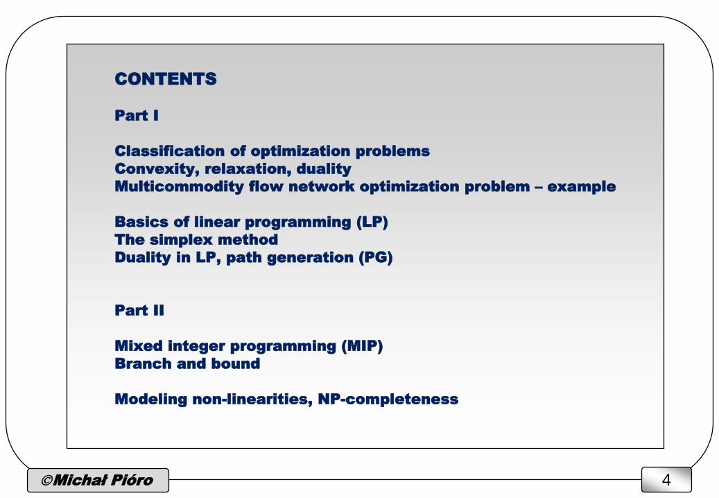
basic notions - examples

intervals (a,b), [a,b], (a,b] in R1

disc in R2: D = { (x1,x2): x12 + x2

2 r2 }, circumference D = { (x1,x2): x12 + x2

2 = r2 }

disc in R2: D = { (x1,x2): x12 + x2

2 < r2 }

simplex in R3: S = {(x1,x2,x3): x1 + x2 + x3 1, x1 0, x2 0, x3 0 }

polyhedron: x Rn: Ax b

functions: quadratic, square root, linear, …

Michał Pióro 7

convexity (concavity)

set X Rn is convex iff

for each pair of points x, y X, the segment [x,y] X, i.e.,

{ (1-)x + y : 0 1 } X

conv(X) – convex hull of (a non-convex) X: the smallest convex set including X

conv(X) – set of all convex combinations of the finite subsets of X

function f: X R is convex (for convex X) iff

for each x, y X and for each scalar (0 1)

f((1-)x + y) (1-)f(x) + f(y)

strictly convex: if < for 0 < < 1

function f: X R is concave (for convex X) if –f is convex

convex continuous

Michał Pióro 8

general form of optimization problems

optimization problem (OP):

minimize F(x) F: X R objective function

x X X Rn optimization space, feasible set

x = (x1,x2,…,xn) Rn variables

convex problem (CXP):

X – convex set

F – convex function

effectively tractable

linear programming (LP) problem

a very special convex problem (X – polyhedron, F – linear function)

efficient methods (simplex method)

non-convex problems

(mixed) integer programming problems (MIP) (LP with discrete variables)

linear constraints and concave objective function (CVP)

Michał Pióro 9

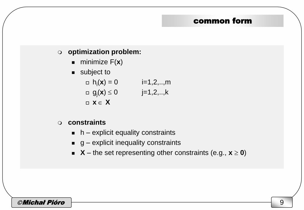
common form

optimization problem:

minimize F(x)

subject to

hi(x) = 0 i=1,2,..,m

gj(x) 0 j=1,2,..,k

x X

constraints

h – explicit equality constraints

g – explicit inequality constraints

X – the set representing other constraints (e.g., x 0)

Michał Pióro 10

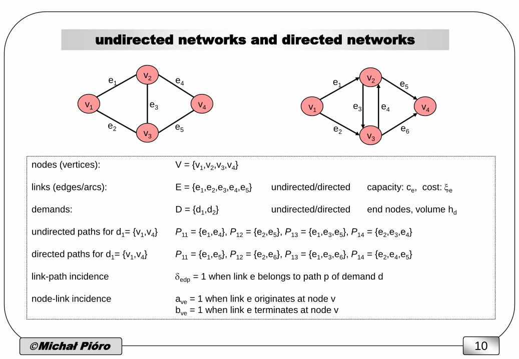
undirected networks and directed networks

nodes (vertices): V = {v1,v2,v3,v4}

links (edges/arcs): E = {e1,e2,e3,e4,e5} undirected/directed capacity: ce, cost: e

demands: D = {d1,d2} undirected/directed end nodes, volume hd

undirected paths for d1= {v1,v4} P11 = {e1,e4}, P12 = {e2,e5}, P13 = {e1,e3,e5}, P14 = {e2,e3,e4}

directed paths for d1= {v1,v4} P11 = {e1,e5}, P12 = {e2,e6}, P13 = {e1,e3,e6}, P14 = {e2,e4,e5}

link-path incidence edp = 1 when link e belongs to path p of demand d

node-link incidence ave = 1 when link e originates at node v

bve = 1 when link e terminates at node v

v2

v1 v4

v3

v2

v1 v4

v3

e1

e2 e5

e4

e3

e1

e2

e3 e4

e5

e6

Michał Pióro 11

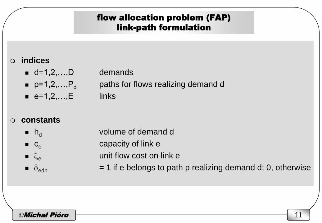
flow allocation problem (FAP)

link-path formulation

indices

d=1,2,…,D demands

p=1,2,…,Pd paths for flows realizing demand d

e=1,2,…,E links

constants

hd volume of demand d

ce capacity of link e

e unit flow cost on link e

edp = 1 if e belongs to path p realizing demand d; 0, otherwise

Michał Pióro 12

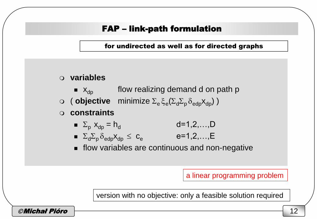
FAP – link-path formulation

variables

xdp flow realizing demand d on path p

( objective minimize Se e(SdSp edpxdp) )

constraints

Sp xdp = hd d=1,2,…,D

SdSp edpxdp ce e=1,2,…,E

flow variables are continuous and non-negative

version with no objective: only a feasible solution required

for undirected as well as for directed graphs

a linear programming problem

Michał Pióro 13

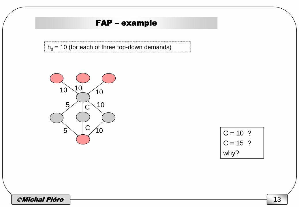
FAP – example

hd = 10 (for each of three top-down demands)

10

5

5

10

10

1010

C

CC = 10 ?

C = 15 ?

why?

Michał Pióro 14

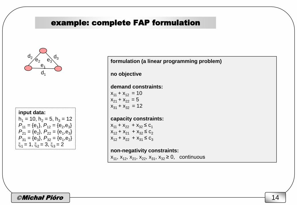
example: complete FAP formulation

input data:

h1 = 10, h2 = 5, h3 = 12

P11 = {e1}, P12 = {e2,e3}

P21 = {e2}, P22 = {e1,e3}

P31 = {e3}, P32 = {e1,e2}

1 = 1, 2 = 3, 3 = 2

formulation (a linear programming problem)

no objective

demand constraints:

x11 + x12 = 10

x21 + x22 = 5

x31 + x32 = 12

capacity constraints:

x11 + x22 + x32 ≤ c1

x12 + x21 + x32 ≤ c2

x12 + x22 + x31 ≤ c3

non-negativity constraints:

x11, x12, x21, x22, x31, x32 ≥ 0, continuous

d1

e3e2

e1

d3d2

Michał Pióro 15

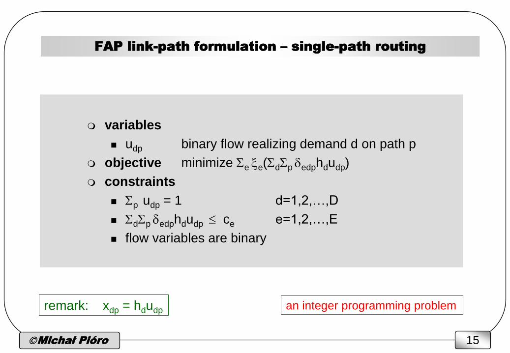
FAP link-path formulation – single-path routing

variables

udp binary flow realizing demand d on path p

objective minimize Se e(SdSp edphdudp)

constraints

Sp udp = 1 d=1,2,…,D

SdSp edphdudp ce e=1,2,…,E

flow variables are binary

an integer programming problemremark: xdp = hdudp

Michał Pióro 16

linear programming -

a problem and its solution

maximize z = x1 + 3x2

subject to - x1 + x2 1

x1 + x2 2

x1 0 , x2 0

x2

x1

-x1+x2 = 1

x1+3x2 =zz=5

z=3

z=0

(1/2,3/2)

extreme point (vertex)

z=2

x1+x2 = 2

Michał Pióro 17

linear programming -

another objective function

maximize z = x1 - x2

subject to - x1 + x2 1

x1 + x2 2

x1 0 , x2 0

x2

x1

-x1+x2 = 1

x1+3x2 =z

z=2

z= -1

z=0

(2,0)

extreme point (vertex)

z=

x1+x2 = 2

Michał Pióro 18

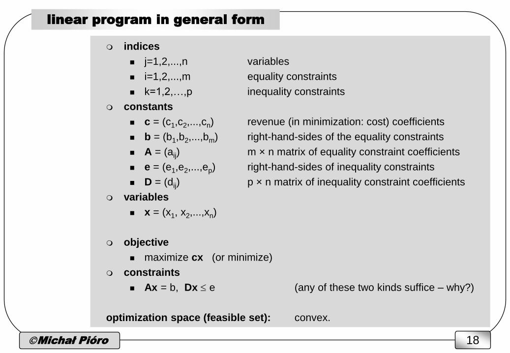
linear program in general form

indices

j=1,2,...,n variables

i=1,2,...,m equality constraints

k=1,2,…,p inequality constraints

constants

c = (c1,c2,...,cn) revenue (in minimization: cost) coefficients

b = (b1,b2,...,bm) right-hand-sides of the equality constraints

A = (aij) m × n matrix of equality constraint coefficients

e = (e1,e2,...,ep) right-hand-sides of inequality constraints

D = (dij) p × n matrix of inequality constraint coefficients

variables

x = (x1, x2,...,xn)

objective

maximize cx (or minimize)

constraints

Ax = b, Dx e (any of these two kinds suffice – why?)

optimization space (feasible set): convex.

Michał Pióro 19

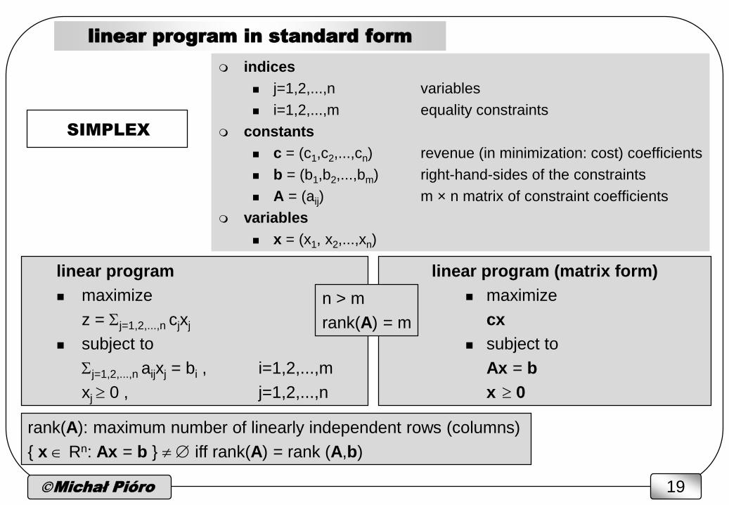
linear program in standard form

indices

j=1,2,...,n variables

i=1,2,...,m equality constraints

constants

c = (c1,c2,...,cn) revenue (in minimization: cost) coefficients

b = (b1,b2,...,bm) right-hand-sides of the constraints

A = (aij) m × n matrix of constraint coefficients

variables

x = (x1, x2,...,xn)

linear program

maximize

z = Sj=1,2,...,n cjxj

subject to

Sj=1,2,...,n aijxj = bi , i=1,2,...,m

xj 0 , j=1,2,...,n

linear program (matrix form)

maximize

cx

subject to

Ax = b

x 0

n > m

rank(A) = m

SIMPLEX

rank(A): maximum number of linearly independent rows (columns)

{ x Rn: Ax = b } iff rank(A) = rank (A,b)

Michał Pióro 20

transformation of LPs to the standard form

slack variables

Sj=1,2,...,n aijxj bi to Sj=1,2,...,n aijxj + xn+i = bi , xn+i 0

Sj=1,2,...,n aijxj bi to Sj=1,2,...,n aijxj - xn+i = bi , xn+i 0

remark: in exercises we will use si instead of xn+i

nonnegative variables

xk with unconstrained sign: xk = xk - xk

, xk 0 , xk

0

exercise: transform the following LP to the standard form

maximize z = x1 + x2

subject to 2x1 + 3x2 6

x1 + 7x2 4

x1 + x2 = 3

x1 0 , x2 unconstrained in sign

Michał Pióro 21

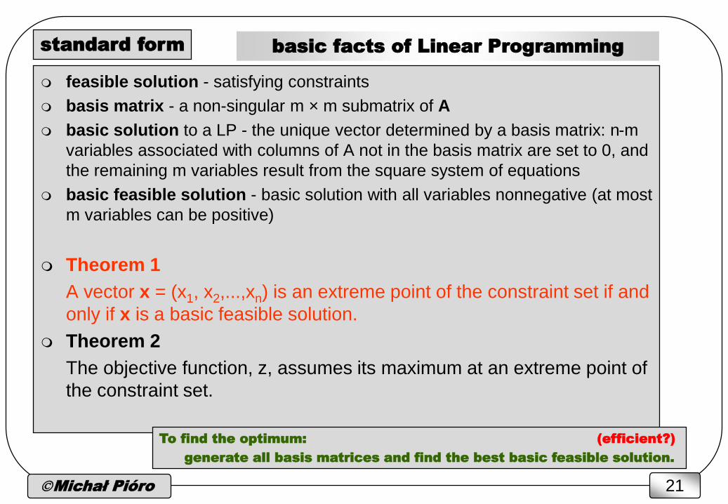
basic facts of Linear Programming

feasible solution - satisfying constraints

basis matrix - a non-singular m × m submatrix of A

basic solution to a LP - the unique vector determined by a basis matrix: n-m

variables associated with columns of A not in the basis matrix are set to 0, and

the remaining m variables result from the square system of equations

basic feasible solution - basic solution with all variables nonnegative (at most

m variables can be positive)

Theorem 1

A vector x = (x1, x2,...,xn) is an extreme point of the constraint set if and

only if x is a basic feasible solution.

Theorem 2

The objective function, z, assumes its maximum at an extreme point of

the constraint set.

standard form

To find the optimum: (efficient?)

generate all basis matrices and find the best basic feasible solution.

Michał Pióro 22

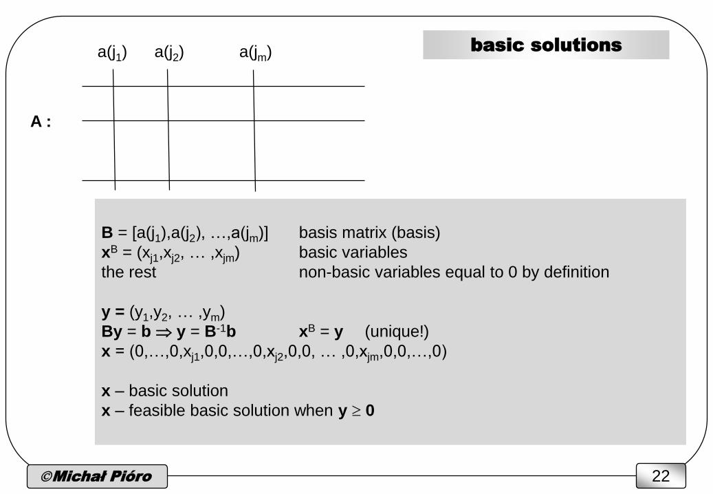
basic solutions

A :

a(j1) a(j2) a(jm)

B = [a(j1),a(j2), …,a(jm)] basis matrix (basis)

xB = (xj1,xj2, … ,xjm) basic variables

the rest non-basic variables equal to 0 by definition

y = (y1,y2, … ,ym)

By = b y = B-1b xB = y (unique!)

x = (0,…,0,xj1,0,0,…,0,xj2,0,0, … ,0,xjm,0,0,…,0)

x – basic solution

x – feasible basic solution when y 0

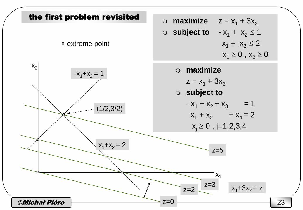
Michał Pióro 23

the first problem revisited maximize z = x1 + 3x2

subject to - x1 + x2 1

x1 + x2 2

x1 0 , x2 0

x2

x1

-x1+x2 = 1

x1+x2 = 2

x1+3x2 = z

z=5

z=3

z=0

(1/2,3/2)

extreme point

maximize

z = x1 + 3x2

subject to

- x1 + x2 + x3 = 1

x1 + x2 + x4 = 2

xj 0 , j=1,2,3,4

z=2

Michał Pióro 24

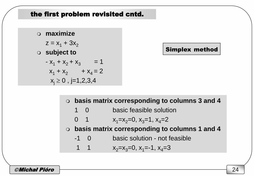
the first problem revisited cntd.

maximize

z = x1 + 3x2

subject to

- x1 + x2 + x3 = 1

x1 + x2 + x4 = 2

xj 0 , j=1,2,3,4

basis matrix corresponding to columns 3 and 4

1 0 basic feasible solution

0 1 x1=x2=0, x3=1, x4=2

basis matrix corresponding to columns 1 and 4

-1 0 basic solution - not feasible

1 1 x2=x3=0, x1=-1, x4=3

Simplex method

Michał Pióro 25

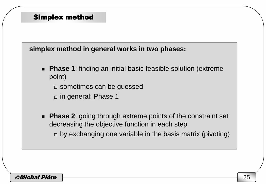
Simplex method

simplex method in general works in two phases:

Phase 1: finding an initial basic feasible solution (extreme

point)

sometimes can be guessed

in general: Phase 1

Phase 2: going through extreme points of the constraint set

decreasing the objective function in each step

by exchanging one variable in the basis matrix (pivoting)

Michał Pióro 26

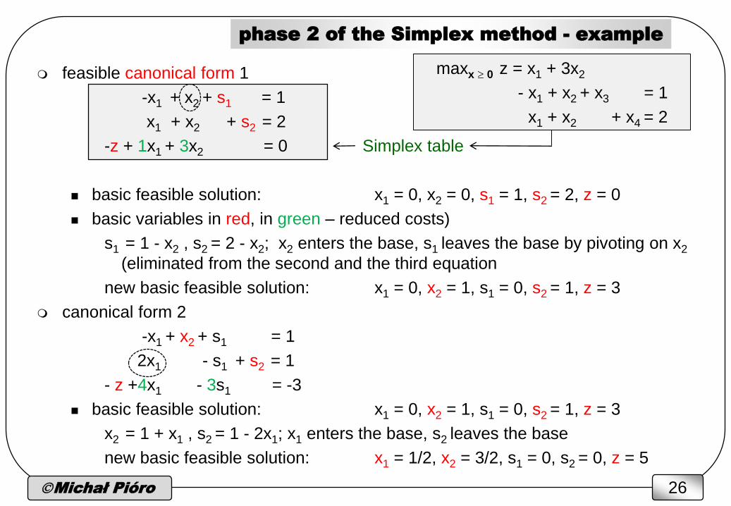
feasible canonical form 1

-x1 + x2 + s1 = 1

x1 + x2 + s2 = 2

-z + 1x1 + 3x2 = 0 Simplex table

basic feasible solution: x1 = 0, x2 = 0, s1 = 1, s2 = 2, z = 0

basic variables in red, in green – reduced costs)

s1 = 1 - x2 , s2 = 2 - x2; x2 enters the base, s1 leaves the base by pivoting on x2

(eliminated from the second and the third equation

new basic feasible solution: x1 = 0, x2 = 1, s1 = 0, s2 = 1, z = 3

canonical form 2

-x1 + x2 + s1 = 1

2x1 - s1 + s2 = 1

- z +4x1 - 3s1 = -3

basic feasible solution: x1 = 0, x2 = 1, s1 = 0, s2 = 1, z = 3

x2 = 1 + x1 , s2 = 1 - 2x1; x1 enters the base, s2 leaves the base

new basic feasible solution: x1 = 1/2, x2 = 3/2, s1 = 0, s2 = 0, z = 5

phase 2 of the Simplex method - example

maxx 0 z = x1 + 3x2

- x1 + x2 + x3 = 1

x1 + x2 + x4 = 2

Michał Pióro 27

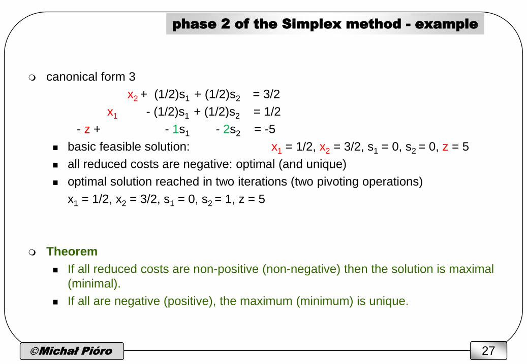
canonical form 3

x2 + (1/2)s1 + (1/2)s2 = 3/2

x1 - (1/2)s1 + (1/2)s2 = 1/2

- z + - 1s1 - 2s2 = -5

basic feasible solution: x1 = 1/2, x2 = 3/2, s1 = 0, s2 = 0, z = 5

all reduced costs are negative: optimal (and unique)

optimal solution reached in two iterations (two pivoting operations)

x1 = 1/2, x2 = 3/2, s1 = 0, s2 = 1, z = 5

Theorem

If all reduced costs are non-positive (non-negative) then the solution is maximal

(minimal).

If all are negative (positive), the maximum (minimum) is unique.

phase 2 of the Simplex method - example

Michał Pióro 28

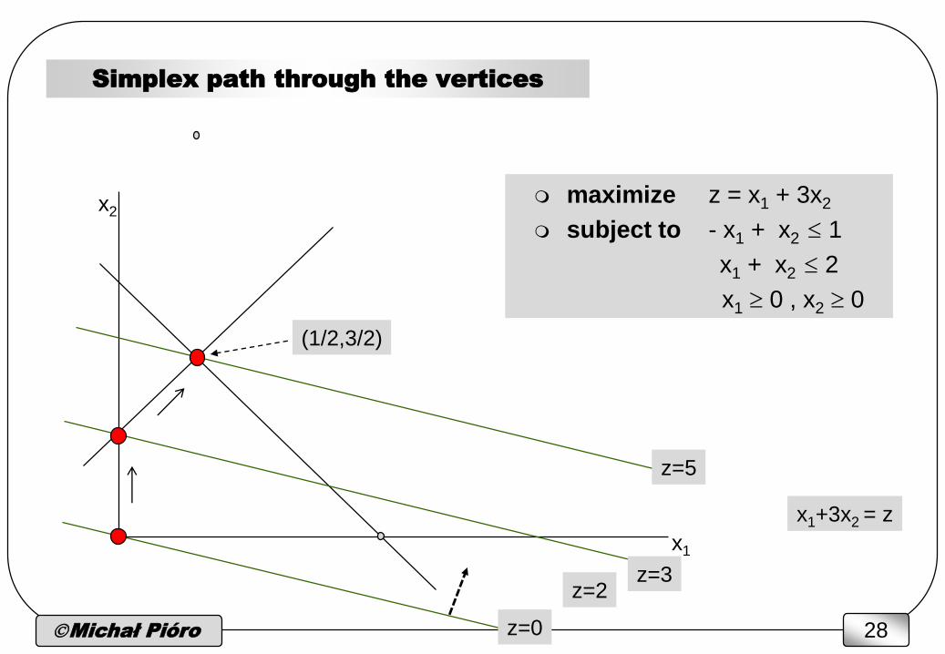
Simplex path through the vertices

maximize z = x1 + 3x2

subject to - x1 + x2 1

x1 + x2 2

x1 0 , x2 0

x2

x1

x1+3x2 = z

z=5

z=3

z=0

(1/2,3/2)

z=2

Michał Pióro 29

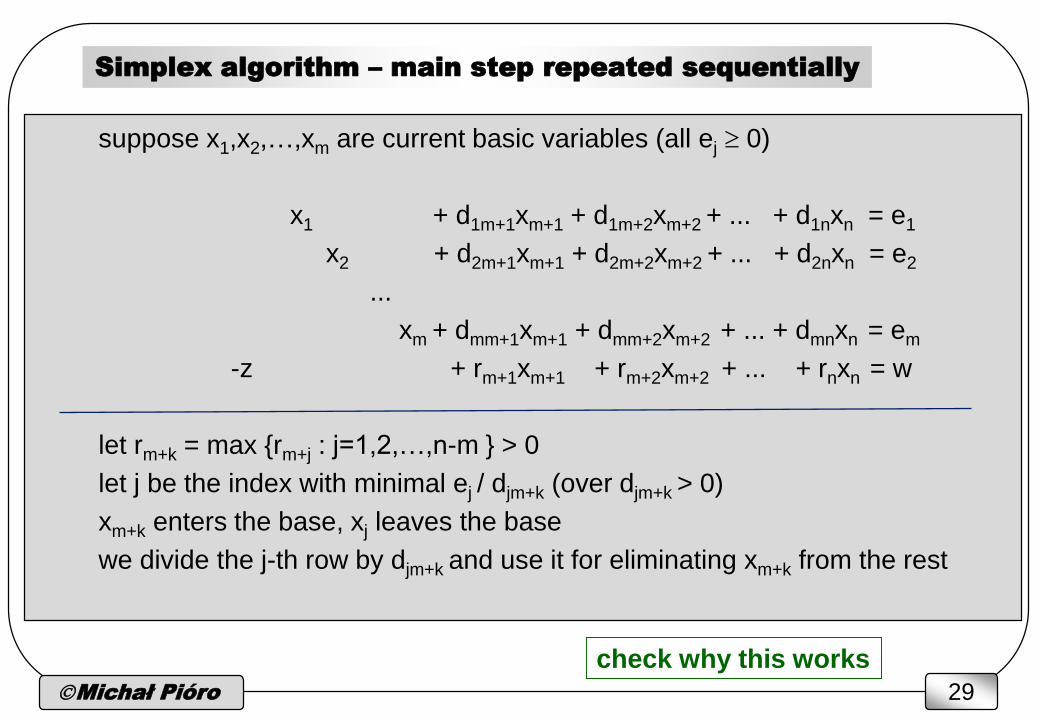
Simplex algorithm – main step repeated sequentially

suppose x1,x2,…,xm are current basic variables (all ej 0)

x1 + d1m+1xm+1 + d1m+2xm+2 + ... + d1nxn = e1

x2 + d2m+1xm+1 + d2m+2xm+2 + ... + d2nxn = e2

...

xm + dmm+1xm+1 + dmm+2xm+2 + ... + dmnxn = em

-z + rm+1xm+1 + rm+2xm+2 + ... + rnxn = w

let rm+k = max {rm+j : j=1,2,…,n-m } > 0

let j be the index with minimal ej / djm+k (over djm+k > 0)

xm+k enters the base, xj leaves the base

we divide the j-th row by djm+k and use it for eliminating xm+k from the rest

check why this works

Michał Pióro 30

Simplex method – phase 1

Phase 1: finding an initial basic feasible solution

minimize xn+1+ xn+2 +...+ xn+m

a11x1+a12x2+...+a1nxn+xn+1 = b1

a21x1+a22x2+...+a2nxn +xn+2 = b2

...

am1x1+am2x2+...+amnxn +xn+m = bm

xj 0 , j=1,2,...,m+n (xn+i - artificial variables)

bi have all been made positive

Remark: We can keep the original objective as an additional row of the

Simplex table. Then we can immediately start Phase 2 once all

artificial variables become equal to 0.

Michał Pióro 31

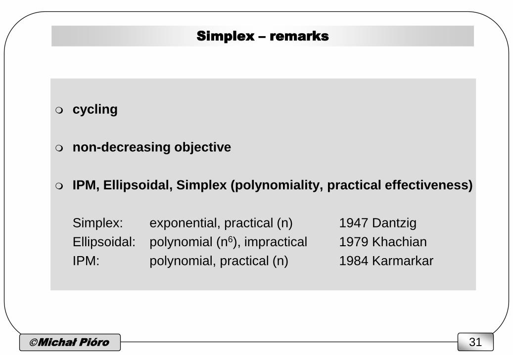
Simplex – remarks

cycling

non-decreasing objective

IPM, Ellipsoidal, Simplex (polynomiality, practical effectiveness)

Simplex: exponential, practical (n) 1947 Dantzig

Ellipsoidal: polynomial (n6), impractical 1979 Khachian

IPM: polynomial, practical (n) 1984 Karmarkar

Michał Pióro 32

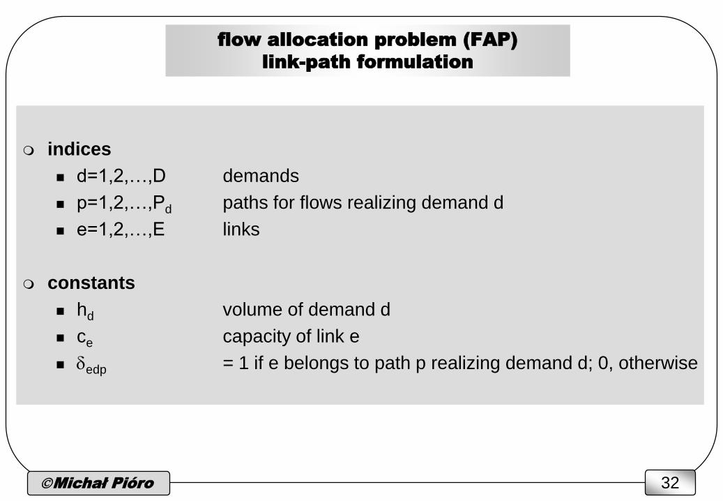
flow allocation problem (FAP)

link-path formulation

indices

d=1,2,…,D demands

p=1,2,…,Pd paths for flows realizing demand d

e=1,2,…,E links

constants

hd volume of demand d

ce capacity of link e

edp = 1 if e belongs to path p realizing demand d; 0, otherwise

Michał Pióro 33

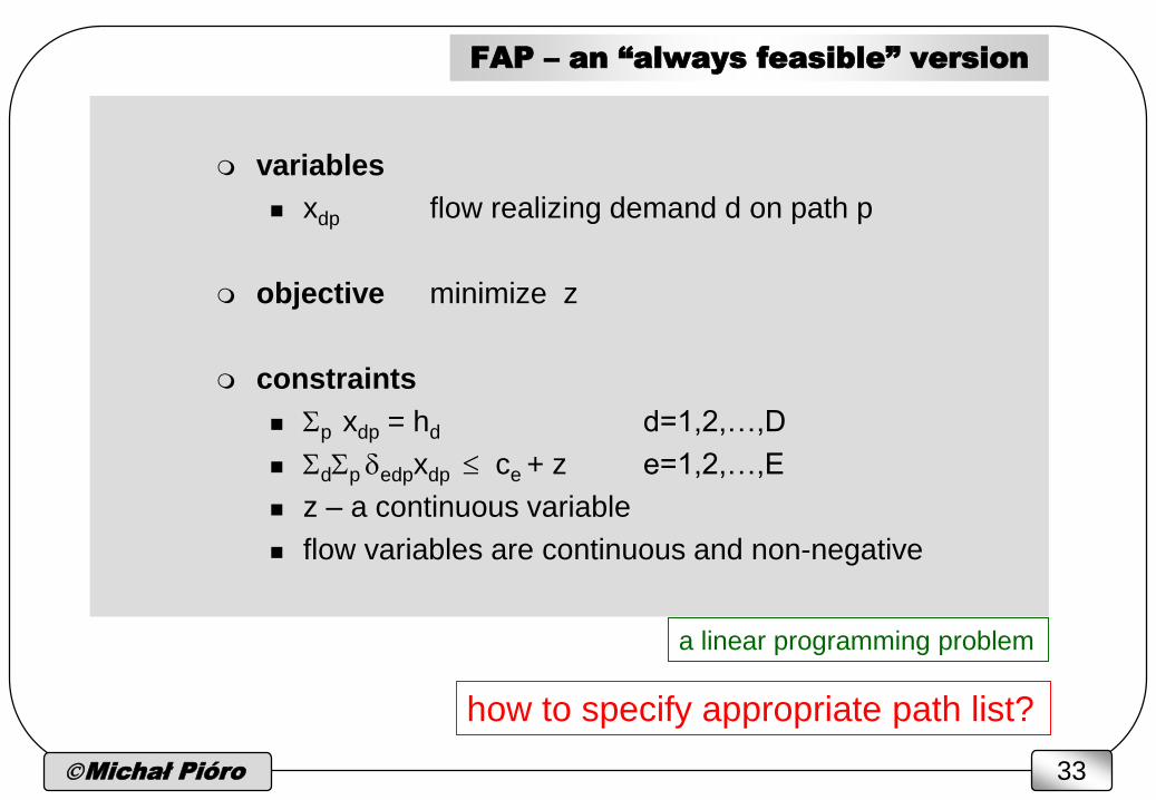
variables

xdp flow realizing demand d on path p

objective minimize z

constraints

Sp xdp = hd d=1,2,…,D

SdSp edpxdp ce + z e=1,2,…,E

z – a continuous variable

flow variables are continuous and non-negative

a linear programming problem

how to specify appropriate path list?

FAP – an “always feasible” version

Michał Pióro 34

example of the difficulty

the number of paths in the graph grows

exponentially so we simply cannot put

them all on the path lists! 5 by 5 Manhattan network (n = 5):

70 shortest-hop paths between two

opposite corners

h = 1 +

c = 1 + c = 1 +

c = 1 + c = 1 + all 10 demands but one with h = 1

all 10 links but four with capacity 1

how should we know that the thick path

must be used to get the optimal solution?

Michał Pióro 35

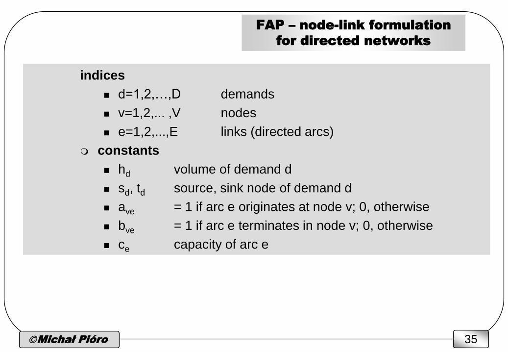
FAP – node-link formulation

for directed networks

indices

d=1,2,…,D demands

v=1,2,... ,V nodes

e=1,2,...,E links (directed arcs)

constants

hd volume of demand d

sd, td source, sink node of demand d

ave = 1 if arc e originates at node v; 0, otherwise

bve = 1 if arc e terminates in node v; 0, otherwise

ce capacity of arc e

Michał Pióro 36

node-link formulation for directed networks

variables

xed 0 flow of demand d on arc e

objective minimize z

constraints

= hd if v = sd

Se ave xed - Se bve xed = 0 if v sd,td

= - hd if v = td

v=1,2,...,V, d=1,2,…,D

Sd xed ce + z e=1,2,…,E

we need to find the path flows (loops possible)xed = Sp edpxdp link flows

Michał Pióro 37

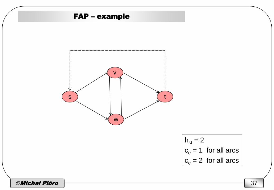
FAP – example

w

v

ts

hst = 2

ce = 1 for all arcs

ce = 2 for all arcs

Michał Pióro 38

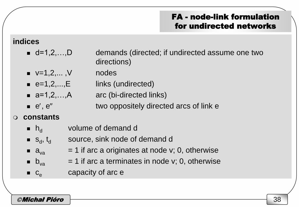
FA - node-link formulation

for undirected networks

indices

d=1,2,…,D demands (directed; if undirected assume one two

directions)

v=1,2,... ,V nodes

e=1,2,...,E links (undirected)

a=1,2,…,A arc (bi-directed links)

e, e two oppositely directed arcs of link e

constants

hd volume of demand d

sd, td source, sink node of demand d

ava = 1 if arc a originates at node v; 0, otherwise

bva = 1 if arc a terminates in node v; 0, otherwise

ce capacity of arc e

Michał Pióro 39

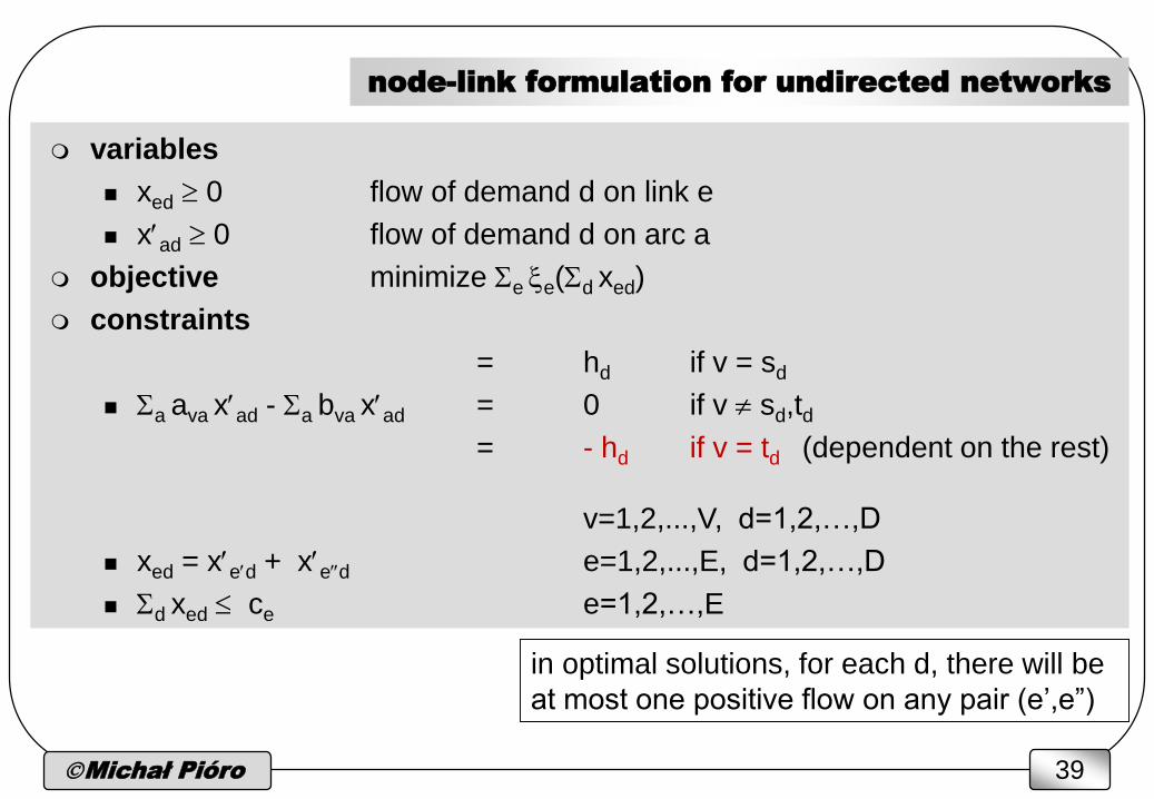
node-link formulation for undirected networks

variables

xed 0 flow of demand d on link e

xad 0 flow of demand d on arc a

objective minimize Se e(Sd xed)

constraints

= hd if v = sd

Sa ava xad - Sa bva xad = 0 if v sd,td

= - hd if v = td (dependent on the rest)

v=1,2,...,V, d=1,2,…,D

xed = xed + xed e=1,2,...,E, d=1,2,…,D

Sd xed ce e=1,2,…,E

in optimal solutions, for each d, there will be

at most one positive flow on any pair (e’,e”)

Michał Pióro 40

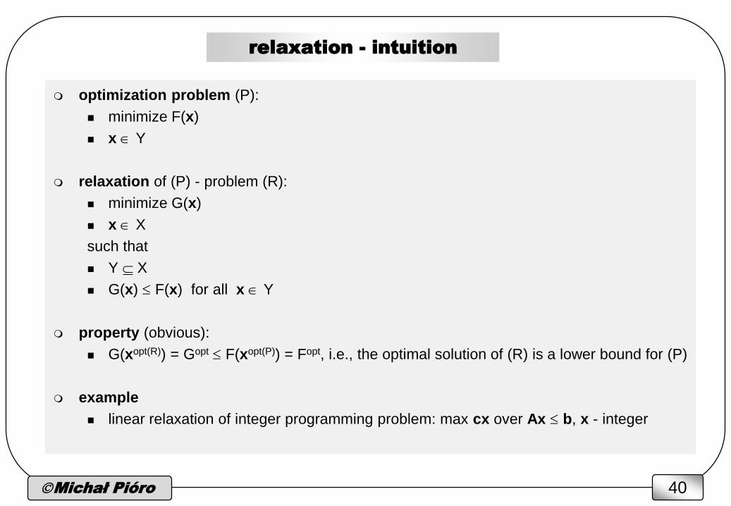
relaxation - intuition

optimization problem (P):

minimize F(x)

x Y

relaxation of (P) - problem (R):

minimize G(x)

x X

such that

Y X

G(x) F(x) for all x Y

property (obvious):

G(xopt(R)) = Gopt F(xopt(P)) = Fopt, i.e., the optimal solution of (R) is a lower bound for (P)

example

linear relaxation of integer programming problem: max cx over Ax b, x - integer

Michał Pióro 41

dual theory

Consider a programing problem (P):

minimize F(x)

subject to

hi(x) = 0 i=1,2,..,k

gj(x) 0 j=1,2,..,m set Y

x X

Form the Lagrangean function:

L(x; ,) = F(x) + i ihi(x) + j jgj(x)

x X, - unconstrained in sign, 0

Define the problem (R(,)):

minx X L(x; ,) this is a relaxation of (P)

Michał Pióro 42

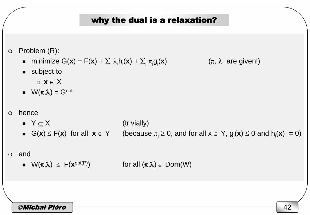
why the dual is a relaxation?

Problem (R):

minimize G(x) = F(x) + i ihi(x) + j jgj(x) (, are given!)

subject to

x X

W(,) = Gopt

hence

Y X (trivially)

G(x) F(x) for all x Y (because j 0, and for all x Y, gj(x) 0 and hi(x) = 0)

and

W(,) F(xopt(P)) for all (,) Dom(W)

Michał Pióro 43

dual problem

Lagrangean function (one vector of primal variables and two vectors of dual

variables)

L(x; ,) = F(x) + i ihi(x) + j jgj(x)

x X, - unconstrained in sign, 0

Dual function:

W(,) = minx X L(x; ,)

- unconstrained in sign, 0

Dom(W) = {(,): - unconstrained in sign, 0, minx X L(x; ,) > - }

note that when X is compact then minx X L(x; ,) > -

Dual problem (D): finding the best relaxation of (P)

maximize W(,)

subject to (,) Dom(W)

Michał Pióro 44

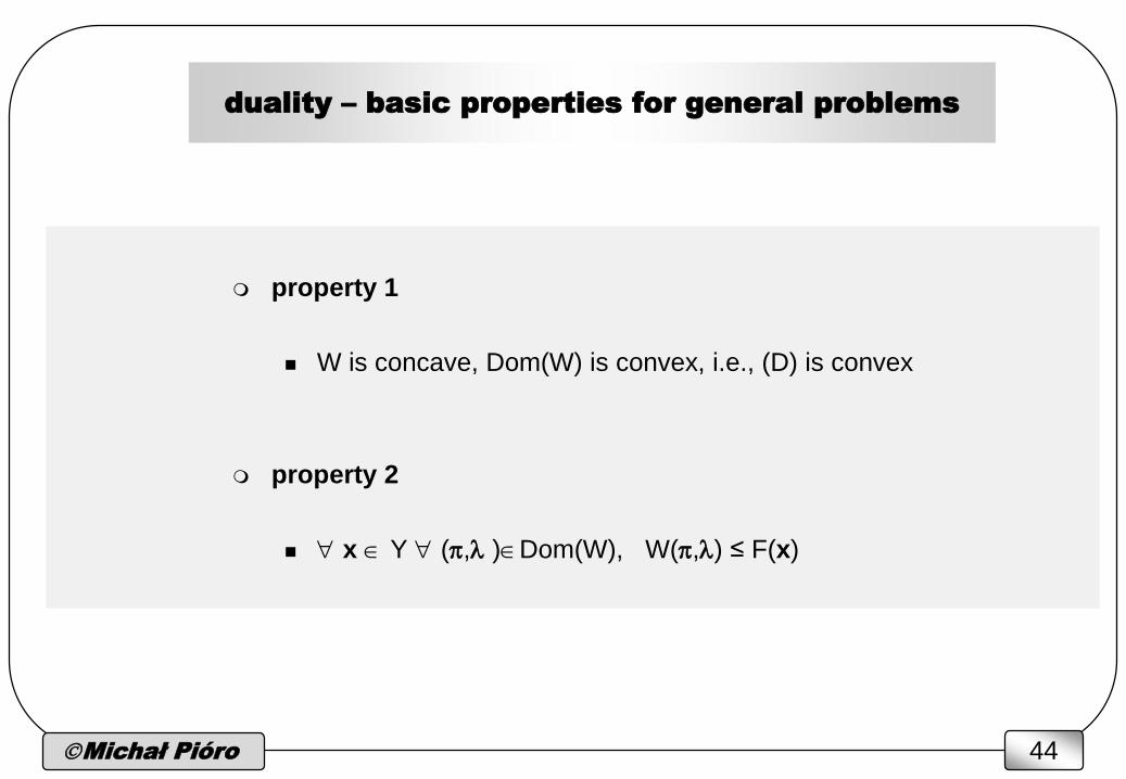
duality – basic properties for general problems

property 1

W is concave, Dom(W) is convex, i.e., (D) is convex

property 2

x Y (, )Dom(W), W(,) ≤ F(x)

Michał Pióro 45

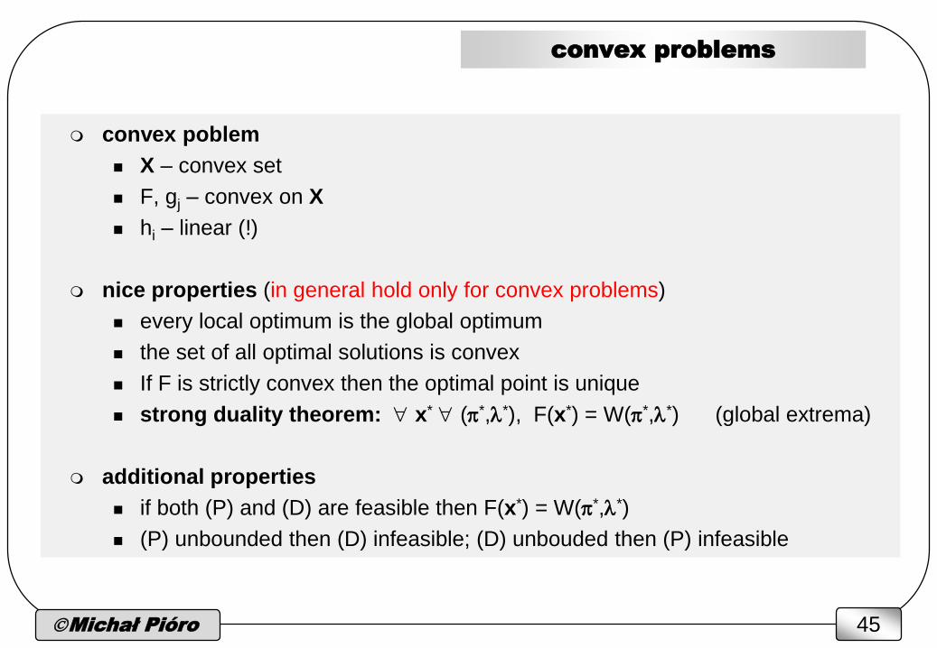
convex problems

convex poblem

X – convex set

F, gj – convex on X

hi – linear (!)

nice properties (in general hold only for convex problems)

every local optimum is the global optimum

the set of all optimal solutions is convex

If F is strictly convex then the optimal point is unique

strong duality theorem: x* (*,*), F(x*) = W(*,*) (global extrema)

additional properties

if both (P) and (D) are feasible then F(x*) = W(*,*)

(P) unbounded then (D) infeasible; (D) unbouded then (P) infeasible

Michał Pióro 47

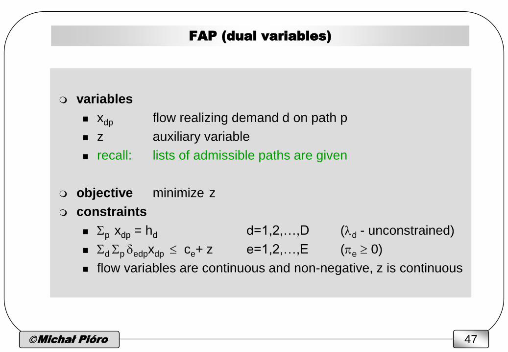
FAP (dual variables)

variables

xdp flow realizing demand d on path p

z auxiliary variable

recall: lists of admissible paths are given

objective minimize z

constraints

Sp xdp = hd d=1,2,…,D (d - unconstrained)

Sd Sp edpxdp ce+ z e=1,2,…,E (e 0)

flow variables are continuous and non-negative, z is continuous

Michał Pióro 48

dual

L(x,z; ,) = z + Sd d(hd - Sp xdp) + Se e(Sd Sp edpxdp - ce- z)

xdp 0 for all (d,p)

W(,) = minx0,z L(x,z; ,)

Dual

maximize W(,) = Sd dhd - Se ece

subject to

Se e = 1

d Se edpe d=1,2,…,D p=1,2,...,Pd

e 0 e=1,2,...,E

for LP there is a receipt for formulating duals

Michał Pióro 49

path generation - the reason

dual

maximize Sd dhd - Se ece

subject to

Se e = 1

d Se edpe d=1,2,…,D p=1,2,...,Pd

e 0 e=1,2,...,E

if we can find a path shorter than d* then we will get a more

constrained dual problem and hence have a chance to improve

(decrease) the optimal dual objective

i.e., to decrease the optimal primal objective

shortest path algorithm can be used for finding shortest paths with

respect to *

Michał Pióro 50

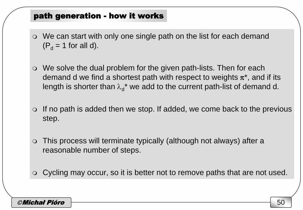
path generation - how it works

We can start with only one single path on the list for each demand

(Pd = 1 for all d).

We solve the dual problem for the given path-lists. Then for each

demand d we find a shortest path with respect to weights *, and if its

length is shorter than d* we add to the current path-list of demand d.

If no path is added then we stop. If added, we come back to the previous

step.

This process will terminate typically (although not always) after a

reasonable number of steps.

Cycling may occur, so it is better not to remove paths that are not used.

Michał Pióro 51

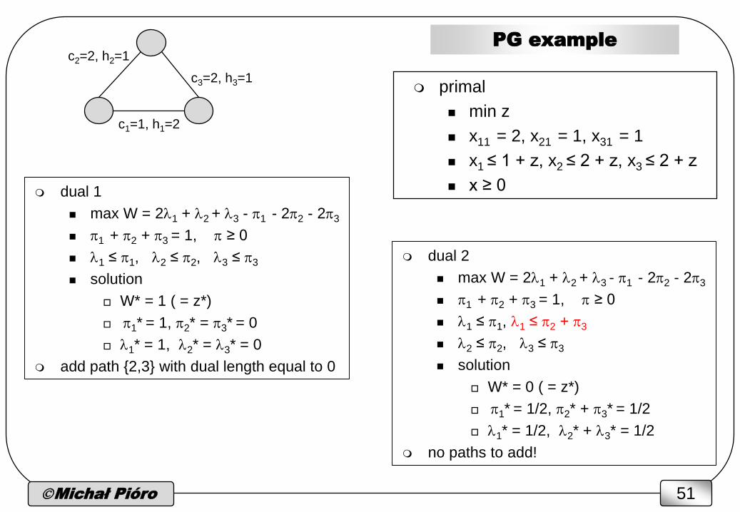
primal

min z

x11 = 2, x21 = 1, x31 = 1

x1 ≤ 1 + z, x2 ≤ 2 + z, x3 ≤ 2 + z

x ≥ 0

PG example

c3=2, h3=1

c1=1, h1=2

c2=2, h2=1

dual 1

max W = 21 + 2 + 3 - 1 - 22 - 23

1 + 2 + 3 = 1, ≥ 0

1 ≤ 1, 2 ≤ 2, 3 ≤ 3

solution

W* = 1 ( = z*)

1* = 1, 2* = 3* = 0

1* = 1, 2* = 3* = 0

add path {2,3} with dual length equal to 0

dual 2

max W = 21 + 2 + 3 - 1 - 22 - 23

1 + 2 + 3 = 1, ≥ 0

1 ≤ 1, 1 ≤ 2 + 3

2 ≤ 2, 3 ≤ 3

solution

W* = 0 ( = z*)

1* = 1/2, 2* + 3* = 1/2

1* = 1/2, 2* + 3* = 1/2

no paths to add!

Michał Pióro 52

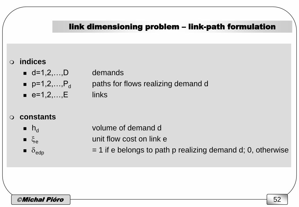
link dimensioning problem – link-path formulation

indices

d=1,2,…,D demands

p=1,2,…,Pd paths for flows realizing demand d

e=1,2,…,E links

constants

hd volume of demand d

e unit flow cost on link e

edp = 1 if e belongs to path p realizing demand d; 0, otherwise

Michał Pióro 53

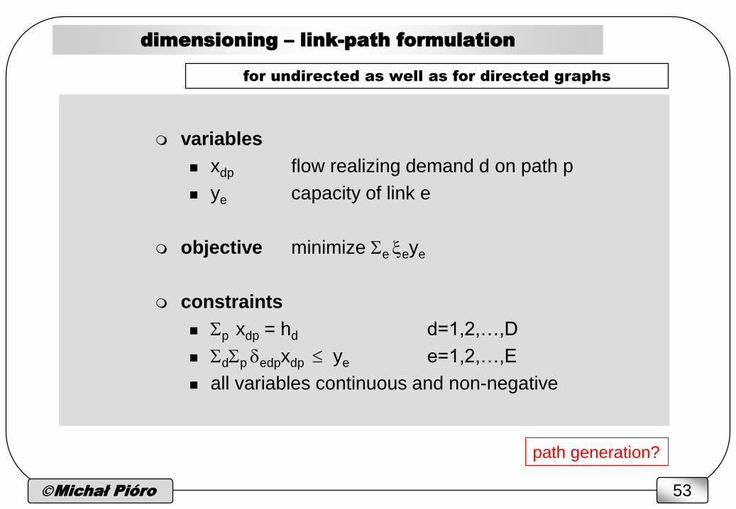
dimensioning – link-path formulation

variables

xdp flow realizing demand d on path p

ye capacity of link e

objective minimize Se eye

constraints

Sp xdp = hd d=1,2,…,D

SdSp edpxdp ye e=1,2,…,E

all variables continuous and non-negative

for undirected as well as for directed graphs

path generation?

Michał Pióro 54

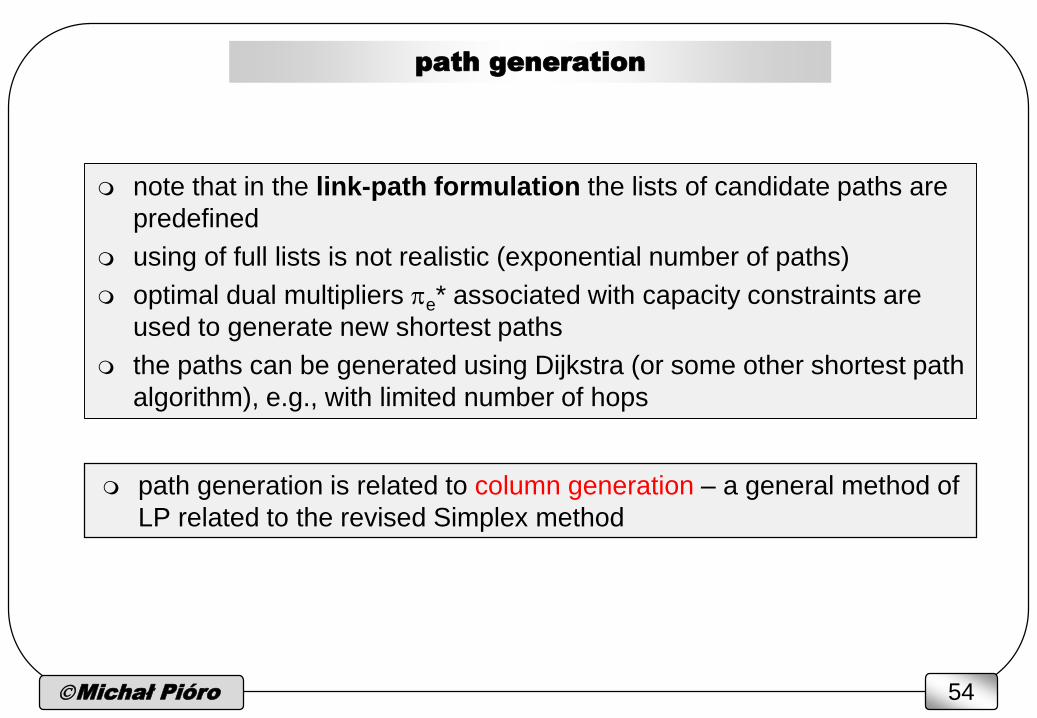
path generation

note that in the link-path formulation the lists of candidate paths are

predefined

using of full lists is not realistic (exponential number of paths)

optimal dual multipliers e* associated with capacity constraints are

used to generate new shortest paths

the paths can be generated using Dijkstra (or some other shortest path

algorithm), e.g., with limited number of hops

path generation is related to column generation – a general method of

LP related to the revised Simplex method

Michał Pióro 55

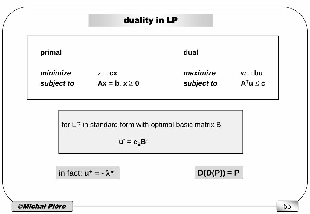
duality in LP

primal dual

minimize z = cx maximize w = bu

subject to Ax = b, x 0 subject to ATu c

for LP in standard form with optimal basic matrix B:

u* = cBB-1

in fact: u* = - * D(D(P)) = P