Embed Size (px)
Citation preview
MPP03 Chap2Bo E. Sernelius 31
Chapter 2
Green's Functions at Zero Temperature
Which is the lowest kinetic temperature ever achieved in a laboratory? Answer: 2.5m K was achieved in 1988 by a group at the Ecole Normale Supérieure: A. Aspect, E.Arimondo, R. Kaiser, N. Vansteenkiste, C. Cohen-Tannoudji, Phys. Rev. Lett. 61, 826 (1988). Since thenthere has been an increased activity in low-temperature physics and the lowest temperature in 1997 is 0.6nK.
The Green's function techniques are used when one can not solve the problem exactly.
Let us assume that we are trying to deduce the properties of a system described by the
Hamiltonian H which may not be solved exactly. The usual approach is to set
H = H0 + V,
where H0 is a Hamiltonian which can be solved exactly. The term V represents all the
remaining parts of H. One tries to choose H0 so that the effects of V are small. The basic
procedure is to start with a system completely described by H0. The effects of V are
introduced, and we try to find how it changes the system we understand. This is the basic
procedure in many-body theory.
2.1. INTERACTION REPRESENTATION
A. Schrödinger
Elementary quantum mechanics is taught in the Schrödinger representation, which is
based on the formula
it
t H th∂∂
j j( ) ( ) ,=
which has the operator formal solution
j j( ) ( ) ./t e iHt= - h 0
The use of this formula requires some assumptions:
1. The wave functions are time dependent.
2. Operators are taken to be independent of time.
MPP03 Chap2Bo E. Sernelius 32
B. Heisenberg
It is possible to solve quantum mechanical problems another way which gives the same
answers but yet uses methods that look quite different. The Heisenberg representation has
the following properties:
1. The wave functions are independent of time.
2. The operators are time dependent, and this dependence is given by
O t e O eiHt iHt( ) ( )/ /= -h h0
or, equivalently, one is trying to solve the equation which is derived from this:
i
tO t O t Hh
∂∂
( ) ( ), .= [ ]
In physics one is usually trying to evaluate matrix elements. In the Schrödinger
representation, the matrix element of the operator O(0) between two states is
j j j j1 2 1 20 0 0 0† † / /( ) ( ) ( ) ( ) ( ) ( ) .t O t e O eiHt iHt= -h h
In the Heisenberg representation one obtains the result
j j j j1 2 1 20 0 0 0 0† † / /( ) ( ) ( ) ( ) ( ) ( ) .O t e O eiHt iHt= -h h
The two representations produce the same results.
C. Interaction
The interaction representation is another way of doing things. Here both the wave
functions and the operators are time dependent. This is done by separating the Hamiltonian
into two parts,
H = H0 + V,
MPP03 Chap2Bo E. Sernelius 33
where H0 is the unperturbed part and V is the perturbation. This separation can be done in
different ways. Usually H0 is selected as the Hamiltonian which is exactly solvable.
Operators and wave functions in the interaction representation will be denoted by a
caret. Their time dependence is given by:
1. Wave functions have a time dependence
ˆ( ) ( ) ( ) ./ / /j j jt e t e eiH t iH t iHt= = -0 0 0h h h (2.13)
2. Operators have a time dependence
ˆ( ) ./ /O t e OeiH t iH t= -0 0h h
In the Heisenberg representation the time dependence was taken away from the wave
functions and was given to the operators. Here, just the part of the time dependence coming
from H0 is transferred.
Let's check if this produces the same matrix elements as before:
ˆ ( ) ˆ( ) ˆ ( ) ( ) ( )
( ) ( ) .
† † / / / / / /
† / /
j j j j
j j
1 2 1 2
1 2
0 0
0 0
0 0 0 0t O t t e e e Oe e e
e Oe
iHt iH t iH t iH t iH t iHt
iHt iHt
= ( )=
- - -
-
h h h h h h
h h
The time dependence of the operators is governed by the unperturbed Hamiltonian, H0:
i
tO t O t Hh
∂∂
ˆ( ) ˆ( ), .= [ ]0
The time dependence of the wave functions is governed by the perturbation, V:
it
t ii
e H H e
e Ve e V e e e
e Ve
iH t iHt
iH t iHt iH t iH t iH t iHt
iH t iH t
V t
h hh
1 244 344
1 244 3
h h
h h h h h h
h h
∂∂
j j
j j
ˆ( ) ( ) ( )
( ) ( )
/ /
/ / / / / /
/ /
ˆ ( )
= -
= = ( )
=
-
- - -
-
0
0 0 0 0
0 0
0
1
0
0 0
444 1 2444 3444h he e
V t t
iH t iHt
t
0 0/ /
ˆ ( )
( )
ˆ( ) ˆ( ).
-
=
j
j
j
We see from Eq. (2.13) that the wave function at time t is obtained from the one at t = 0 by
MPP03 Chap2Bo E. Sernelius 34
operating with the time development operator U(t):
U t e eiH t iHt( ) / /= -0 h h .
This function has the value unity at t = 0:
U( ) .0 1=
Furthermore, it obeys the following differential equation:
itU t V t U th
∂∂
( ) ˆ( ) ( ).=
We wish to solve this equation. One way of proceeding is by integrating both sides of the
equation with respect to time:
U t Ui
dt V t U t
U ti
dt V t U t
t
t
( ) ( ) ˆ( ) ( )
( ) ˆ( ) ( ).
- = -
fl
= -
Ú
Ú
0
1
0 1 1 1
0 1 1 1
h
h
If this equation is repeatedly iterated, we get
U ti
dt V ti
dt dt V t V t
idt dt dt V t V t V t
t t t
n
nt t t
n nn
( ) ˆ( ) ˆ( ) ˆ( )
ˆ( ) ˆ( ) ˆ( ) .
= - + -ÊË
ˆ¯ +
= -ÊË
ˆ¯
Ú Ú Ú
Â Ú Ú Ú=
•-
10 1 1
2
0 1 0 2 1 2
00 1 0 2 0 1 2
1
1 1
h hL
hL L
Now we introduce the Time ordering operator T. It acts upon a group of time-dependent
operators and is just an instruction to arrange the operators with the earliest times to the right.
For example,
T V t V t V t V t V t V t if t t tˆ( ) ˆ( ) ˆ( ) ˆ( ) ˆ( ) ˆ( ) .1 2 3 3 1 2 3 1 2[ ] = > >
It helps to introduce the following step function:
MPP03 Chap2Bo E. Sernelius 35
q( )
.
x if x
if x
if x
= >= <
= =
1 0
0 0
12
0
Thus for two operators, the explicit definition of T ordering gives
T V t V t t t V t V t t t V t V tˆ( ) ˆ( ) ( ) ˆ( ) ˆ( ) ( ) ˆ( ) ˆ( ) .1 2 1 2 1 2 2 1 2 1[ ] = - + -q q
Now we rearrange the integral by using the above identity:
12
12
120 1 0 2 1 2 0 1 0 2 1 2 0 2 0 1 2 1
1 2
!ˆ( ) ˆ( )
!ˆ( ) ˆ( )
!ˆ( ) ˆ( ) .dt dt T V t V t dt dt V t V t dt dt V t V t
t t t t t t
Ú Ú Ú Ú Ú Ú[ ] = +
The terms on the right hand side are equal. Thus we get
12 0 1 0 2 1 2 0 1 0 2 1 2
1
!ˆ( ) ˆ( ) ˆ( ) ˆ( ) .dt dt T V t V t dt dt V t V t
t t t t
Ú Ú Ú Ú[ ] =
Similarly we can show that
10 1 0 2 0 1 2
0 1 0 2 0 1 21 1
ndt dt dt T V t V t V t
dt dt dt V t V t V t
t t tn n
t t tn n
n
!ˆ( ) ˆ( ) ˆ( )
ˆ( ) ˆ( ) ˆ( ) .
Ú Ú Ú
Ú Ú Ú
[ ]= -
L L
L L
Now, have we reordered the operators from right to left in ascending time order, or
have we just reordered the time arguments? It is difficult to tell straight away since the
operators are all the same in this case. Performing the same derivation as above but for
different operators we find the answer. The answer is that we have just reordered the time
arguments. When the operators are all the same it is just a question of semantics. We can
equally well regard the reordering as a rearrangement of the operators. The time ordering
operator is really an operator that rearranges the order of the operators. We will come back to
this later.
If we now return to our expansion of U(t), we obtain
U ti
ndt dt dt T V t V t V t
Ti
dt V t
n
nt t t
n n
t
( )!
ˆ( ) ˆ( ) ˆ( )
exp ˆ( ) .
= +-( ) [ ]
= -ÊË
ˆ¯
ÈÎÍ
˘˚̇
=
•
Â Ú Ú Ú
Ú
11
0 1 0 2 0 1 2
1 10
hL L
h
(2.1.6)
MPP03 Chap2Bo E. Sernelius 36
2.2 S MATRIX
The time development operator takes the wave function from zero time to the time t.
Now we introduce a more general operator that takes the wave function from t' to t. Since it
has two arguments it is called a matrix, the S matrix S(t,t'):
ˆ( ) ( , ' ) ˆ( ' ) .j jt S t t t=
Now, this operator is closely related to the operator U:
U t t S t t t S t t U t
U t S t t U t
S t t U t U t
( ) ˆ( ) ˆ( ) ( , ' ) ˆ( ' ) ( , ' ) ( ' ) ˆ( )
( ) ( , ' ) ( ' )
( , ' ) ( ) ( ' ) .†
j j j j0 0= = =
fl=
fl
=
We have in the last step used the fact that U is a unitary operator, i.e. U†U = 1. The S matrix
has the following properties:
1. S(t,t) = 1.
2. S†(t,t') = S(t',t)
3. S(t,t')S(t ',t'') = S(t,t'')
4. S(t,t') can be expressed as a time-ordered operator,
∂∂ t
S t ti
V t S t t( , ' ) ˆ( ) ( , ' ) ,= -h
which has the solution
S t t T
idt V t
t
t( , ' ) exp ˆ( ) .
'= -Ê
ˈ¯
ÈÎÍ
˘˚̇Úh
1 1(2.2.1)
At t = 0 the wave functions (and operators) in the three representations coincide. At
zero temperature the only wave function of special interest is the ground state wave function.
The things we want to calculate are expressed as ground-state expectation-values. For our
Green's functions we shall need to define j(0) as the exact ground state wave function.
MPP03 Chap2Bo E. Sernelius 37
Since the total Hamiltonian is H, the exact ground state must have the lowest eigenvalue of
this Hamiltonian. The problem is that we do not know any eigenvalues or eigenstates of this
Hamiltonian. This is one of the things we want to calculate.
Thus we have the problem that all our formalism is based on the wave function which
we do not yet know. The only ground state wave function we know is that of H0, f0.
Somehow we have to determine the unknown wave function j(0) in terms of the known
function f0. This relation was shown by Gell-Mann and Low to be:
j f( ) ( , ) .0 0 0= -•S
We assume that there is no perturbation to start with. Then the system is in the ground state
of H0. At t = - • the perturbation is gradually turned on and the system develops
adiabatically into the state j(0). We also have to bother about the other extreme time limit.
One way is to assume that the interaction is slowly turned off again in the future. Then the
system will return to the noninteracting ground state (at least if f0 is nondegenerate). This
state can differ from f0 by at most a phase factor:
e S SiLf j j f0 00 0= • = • = • -•ˆ( ) ( , ) ( ) ( , ) ,
and
e SiL = • -•f f0 0( , ) .
We should remember that we make the basic assumption that the system develops
adiabatically from the noninteracting ground state into the interacting ground state; we
exclude symmetry breaking, phase transitions and chaotic behavior.
2.3. GREEN'S FUNCTIONS
In this section we will discuss electron and phonon Green's functions. The photon
case is very similar to that for phonons, but more complicated due to the various choices of
gauge. The photon is treated in section 2.10 of the text book.
The electron part of the Hamiltonians we have discussed before are valid not only for
electrons but for all fermions, e.g. 3He. The only difference is in the summation over a
different set of spin quantum numbers. It is furthermore valid for "real" bosons, e.g. 4He.
The phonons and photons are massless bosons, which leads to the possibility that the
number of particles changes – the Hamiltonian contains parts where these particles are
created or annihilated. The operators for particles with mass always appear as products of
MPP03 Chap2Bo E. Sernelius 38
one creation and one destruction operator – this means that one particle is transferred from
one state to another, not created or annihilated. We will now first discuss the electron
Green's function. This discussion is also valid for other fermions with proper modification
in the spin summations. It is slightly different for bosons with mass. Where these differences
occur we will point them out.
Electrons: At zero temperature the electron Green's function is defined as
G t t i Tc t c t( , ' ) ( ) ( ' ) .†l l l- = -
The quantum numbers l can be anything depending on the problem of interest, but often we
will take it to be the quantum numbers of the free-electron gas l = (p,s). Some statements
are needed:
1. The Green's function is expressed in the Heisenberg picture; this means that the states
are time independent and the time dependence of the operators is given by
c t e c eiHt iHtl l( ) ./ /= -h h
2. The state | > is the interacting ground state, i.e., the eigenstate of H with lowest
energy.
3. The operators cl are defined in terms of the complete set of states fl, which are
eigenstates to the unperturbed Hamiltonian H0; we are supposed to know these states.
4. The time-ordering operator T is slightly generalized. The operator acting on several
operators orders them from right to left in ascending order and adds a factor (-1)P,
where P is the number of interchanges of fermion operators from the original given
order. This definition agrees with the earlier one, because the V's that we considered
earlier in connection with the T operator contain an even number of fermion operators.
Thus each permutation of the V's means an even number of permutations of fermion
operators and hence no sign change.That the result changes sign for each permutation
of fermion operators means that the results for fermions and bosons are different.
Let us try to get some feeling for what the Green's function means. For t > t' we have
G t t i c t c t( , ' ) ( ) ( ' ) .†l l l> = -
MPP03 Chap2Bo E. Sernelius 39
At t' a particle is added to the system. After this time the system develops in time. Since the
new state is not an eigenstate of H the added particle scatters into other single particle states.
There is some probability that the particle is still in state l at time t. The Green's function is
just the projection of the state on the state c tl† ( ) , i.e. it is related to the probability that the
electron that was put in state l at t' is still in the same state at t.
For the other time arrangement t' > t we have
G t t i c t c t( , ' ) ( ' ) ( ) ,†l l l> = +
where we have changed the sign since two fermion operators have changed position. At t an
electron is removed from the system and put back at t'. The Green's function is a measure of
the probability that the state l is still empty at t'. Another way to look upon this is that we
create a hole at time t in state l and the Green's function is a measure of the probability that
the hole is still in state l at t'.
Now, we wish to express the Green's function in known quantities; instead of the
interacting ground state we want to use the noninteracting or unperturbed ground state | >0,
i.e. the ground state of H0; thus
= -•S( , ) .00
Next we change the operators to the interaction representation:
c t e e c t e e U t c t U t
S t c t S t
iHt iH t iH t iHtl l l
l
( ) ˆ ( ) ( ) ˆ ( ) ( )
( , ) ˆ ( ) ( , ) ,
/ / / / †= ==
- -h h h h0 0
0 0which leads to:
G t t i t t S S t c t S t S t c t S t S
i t t S S t c t S t S t
( , ' ) ( ') ( , ) ( , ) ˆ ( ) ( , ) ( , ' ) ˆ ( ' ) ( ' , ) ( , )
( ' ) ( , ) ( , ' ) ˆ ( ' ) ( ' , ) ( , ) ˆ
†
†
l q
q
l l
l
- = - - -• -•
+ - -•
0 0
0
0 0 0 0 0 0
0 0 0 0 cc t S t Sl ( ) ( , ) ( , ) .0 00
-•
The time arguments in this expression goes from -• to 0; from 0 to the earliest of t and t';
from that time to 0; from 0 to the latest of t and t'; from that time to 0; from 0 to -•. We want
to rewrite the expression in such a way that the time arguments are increasing. We learned
from the previous section that
MPP03 Chap2Bo E. Sernelius 40
S e S
S
S
iL( , ) ( , )
( , )
( , ).
• -• = = • -•
fl
=• -•
• -•
0 0 0 0 0
00
0 0
Similarly, we find
00
0 0
=• -•
• -•S
S
( , )
( , ).
We use this to replace the left brackets in the expression for the Green's functions and find
G t ti t t
SS S S t c t
S t S t c t S t S
S t
S t t
( , ' )( ' )
( , )( , ) ( , ) ( , ) ˆ ( )
( , ) ( , ' ) ˆ ( ' ) ( ' , ) ( , )
( , )
†
( , ' )
l ql
l
- = - -• -•
• -• -•
¥ -•
•0 0
0
0
0 0
0 0 0 0
1 24444 34444
1 244 3444 1 244 344
1 24444 34444
S t
S t
S t
i t t
SS S S t c t
S t S t c t S t S
( ' , )
†
( , ' )
(
( ' )( , )
( , ) ( , ) ( , ' ) ˆ ( ' )
( ' , ) ( , ) ˆ ( ) ( , ) ( , ) .
-•
•
+ -• -•
• -• -•
¥ -•
ql
l
0 00
0
0 0
0 0 0 0
'' , ) ( , )t S t
1 244 344 1 244 344
-•
Thus, the Green's function can be rewritten as:
G t ti t t
SS t c t S t t c t S t
i t t
SS t c t S t t c t S t
( , ' )( ' )
( , )( , ) ˆ ( ) ( , ' ) ˆ ( ' ) ( ' , )
( ' )( , )
( , ' ) ˆ ( ' ) ( ' , ) ˆ ( ) ( , ) .
†
†
l q
q
l l
l l
- = - -• -•
• -•
+ -• -•
• -•
0 00 0
0 00 0
This can be expressed as

MPP03 Chap2Bo E. Sernelius 41
G t ti Tc t c t S
S( , ' )
ˆ ( ) ˆ ( ' ) ( , )
( , ).
†
l l l- =- • -•
• -•0 0
0 0
(2.3.2)
The operator S(•,-•) contains operators which act in the three time intervals [-•, min(t,t')],
[min(t,t'), max(t,t')], and [max(t,t'), •]. The T operator automatically sorts these so that
they act in their proper sequences. It does not matter where we write S(•,-•) in the
numerator, since the time ordering operator puts the pieces in the right place.
A Green's function can also be defined for the special case where the interactions V = 0
and hence the S matrix is unity. This Green's function, the noninteracting Green's function,
plays a special role in the formalism, and we designate it by G(0):
G t t i Tc t c t( ) †( , ' ) ˆ ( ) ˆ ( ' ) .00 0
l l l- = -
It is also known under the name the unperturbed Green's function or free propagator.
There are two quite different types of electronic systems in which we want to employ
the Green's function analysis. These two have quite different noninteracting and interacting
ground states. These two systems are the following.
1. An Empty Band. Here we wish to study the properties of an electron in an energy
band in which it is the only electron. An example is when we put an electron in the
conduction band of a semiconductor or an insulator. In this case the ground state is the
particle vacuum, which we denote as |0>. This state has the property that
c
a
p
q
0 0
0 0
=
= ,
where cp and aq are destruction operators for electrons and phonons, respectively.
Therefore both H0 and V give zero when operating upon the vacuum. It follows that the S
matrix gives unity when operating upon the vacuum:
S t( , ) .-• =0 0
This means that both of the ground states, |>0 and |>, are the vacuum. The Green's function
can exist only for the time ordering
G t t i t t c t c t( , ' ) ( ' ) ( ) ( ' ) .†l q l l- = - -
MPP03 Chap2Bo E. Sernelius 42
The unperturbed Green's function G(0) is particularly easy to evaluate:
G t t i t t e c c
i t t e
i t t
i t t
( ) ( ' ) / †
( ' ) /
( , ' ) ( ' )
( ' ) .
0 0 0l q
q
el l
e
l
l
- = - -
= - -
- -
- -
h
h
The Fourier transform of G(0)(l,t) with respect to t is defined as
G dte G ti t( , ) ( , ) .l w lw=-•
•Ú
To make the integrals converge, we need to add the infinitesimal quantity id to the
exponents4:
G i dte
Gi
i t i( ) ( / )
( )
( , )
( , )/
.
0
0
0 1
l w
l ww e d
w e d
l
l= -
=- +
• - +Ú h
h
2. A Degenerate Electron Gas. Our second example is where the electrons are in a
Fermi sea at zero temperature. The standard example is a simple metal. It can also be a
heavily doped semiconductor. The system has a chemical potential m, and all electron states
with E < m are occupied. If the unperturbed electrons (eigenstates of H0) are characterized by
an energy ek,s, the ground state |>0 has all states ek,s < m filled and states ek,s > m empty.
The ground states |> and |>0 are no longer the same. The unperturbed ground state can still be
considered as the particle vacuum if we consider particles above m to be electrons and
particles below m to be holes. Processes where an electron below m is scattered to a state
above m is then regarded as a creation of an electron-hole pair. It is convenient to measure the
electron's energy relative to the chemical potential, to define xk,s = ek,s - m. Sometimes we
use m as a reference energy and sometimes we use the bottom of the band. With m as a
reference energy we obtain
0 0
0 0
1
1
1
c ce
n
c c n
F
F
k k k
k k k
k,
†, ,
, ,†
,
,( )
( ) .
s sb bx s
s s s
sx
x
=+
∫
= -
Æ•lim
4This is not just a mathematical trick. The Green's functions we get when including these infinitesimalid's is the limit of the interacting ones when the interactions go to zero. We can never have exactly zerointeraction or expressed in another way: an electron placed in a certain state will not stay there for ever. Thuswe have taken the proper limit.

MPP03 Chap2Bo E. Sernelius 43
The unperturbed Green's function is now
G t t i Tc t c t
i t t n t t n eF Fi t t
s s s
s sxq x q x s
( ), ,
†
, ,( ' ) /
( , ' ) ( ) ( ' )
( ' ) ( ) ( ' ) ( ) .,
00 0
1
k k k
k kk
- = -
= - - -( ) - -[ ] - - h
The first part of this function gives contribution for states outside the Fermi sea and is the
same as the empty-band Green's function. The second part gives contribution only if the
state is within the Fermi sea. The first term can be regarded as the electron part of the
Green's function and the second term as the hole part.
The Fourier transformed Green's function is
G i n dte n dte
Gn
i
n
Fit i
Fit i
F F
s sw x d
sw x d
ss
s
w x x
wx
w x dx
s s( ),
( / ),
( / )
( ) ,
,
,
( , ) ( ) ( )
( , )( )
/
(
, ,0
0
0
0
1
1
k
k
k k
k
k
k
k k= - -( ) -ÈÎÍ
˘˚̇
=- -
+-
• - +-•
- -Ú Úh h
hss
sw x d)
/,- +k h i
We have here added a +id in the electron part and a -id in the hole part5.
Another, more compact way to write G(0) is
Gi
sgnss s
s sww x d
d d x( )
, ,, ,( , )
/; ,0 1
kk k
k k=- +
=h
where dk,s is a small infinitesimal part which changes sign at the chemical potential. It is in
some situations preferable to use the form in the box. If we want to study single-particle
excitations of the ground state, |>0 is replaced by a state with an electron outside and a hole
inside the Fermi sea. The expression inside the box is now valid if the occupation numbers
are properly modified.
Phonons: The Green's function for phonons is defined as
D t t i TA t A t
A a a
( , ; ' ) ( ) ( ' ) ;, ,
, , ,†
q q q
q q q
l l l
l l l
- = -
= +
-
-
The subscript l refer to the polarization of the phonons. Usually we are interested in just one
5See footnote 4. Here the id's guarantee that an electron or a hole placed in a certain state will not stay inthe same state for ever.
MPP03 Chap2Bo E. Sernelius 44
kind of phonon with Hamiltonians which do not mix polarizations, so we shall omit these
subscripts entirely. In the interaction representation one obtains the result
D t t iTA t A t S
S( , ' )
ˆ ( ) ˆ ( ' ) ( , )
( , ).q
q q- = -• -•
• -•-0 0
0 0
At zero temperature there are no phonons. Thus the ground states |> and |>0 are again the
particle vacuum |0>. Note that in an electron-phonon system the notation |>0 means the
combination of ground states for electrons, phonons, etc. Although the phonon system has
the vacuum as its ground state, either of the two electron ground states can be used.
The unperturbed phonon Green's function is defined as
D t t i TA t A t
i T a e a e a e a e
i t t e a a e
i t i t i t i t
i t t i t t
( )
† ' † '
( ' ) † (
( , ' ) ˆ ( ) ˆ ( ' )
( ' )
00 0
0 0
0 0
q q q
q q q q
q q
q q q q
q q
- = -
= - +( ) +( )= - - +
-
-- -
-
- - -
w w w w
w wq '' ) †
( ' ) † ( ' ) †( ' ) .
0 0
0 0 0 0
a a
t t e a a e a ai t t i t t
- -
- - -- -
[ ]{+ - +[ ]}
q q
q q q qq qq w w
Now,
0 0 0 0
0 0 0 0
1
1
1
a a a ae
N
a a a a N
q q q q q
q q q q q
q
† †
† † .
= =-
∫
= = +
- -
- -
bw
Thus,
D t t i N e N ei t t i t t( ) ' '( , ' ) .0 1q q qq q- = - +( ) +[ ]- - -w w
The Fourier transform6 gives
D Ni i
Ni i
( )( , )
.
0 11 1
1 1
q qq q
qq q
ww w d w w d
w w d w w d
= - +( ) + --
- +È
ÎÍÍ
˘
˚˙˙
-- -
-+ +
È
ÎÍÍ
˘
˚˙˙
6To show this is left as homework problem number 7.
MPP03 Chap2Bo E. Sernelius 45
We have here kept the phonon occupation numbers to be able to treat situations where a
phonon is present in the system or we have a finite temperature. For zero temperature and in
the ground state we have Nq = 0, which means that
Di i
i
( )( , )
.
0
2 2
1 1
2
qq q
q
q
ww w d w w d
ww w d
=- +
-+ -
=- +
2.4. WICK'S THEOREM
The Green's function is evaluated by expanding the S matrix S(•,-•) in (2.3.2) in a
series such as (2.2.1):
iG t ti
nd t d t
Tc t V t V t V t c t
S
s
n
nn
s n s
( , ' )( )
!
ˆ ( ) ˆ( ) ˆ( ) ˆ( ) ˆ ( ' )
( , ).
, ,†
p
p p
- = -
¥• -•
=-•
•
-•
•Â Ú ÚhL
L
01
0 1 2 0
0 0
(2.4.1)
Let us for the moment ignore the factor 0<| S(•,-•) |>0. We shall take care of it in Sec. 2.6.
Our immediate aim is to learn how to evaluate time ordered brackets like
0 1 2 3 0Tc t V t V t V t c ts sˆ ( ) ˆ( ) ˆ( ) ˆ( ) ˆ ( ' ) ., ,
†p p (2.4.2)
Suppose that V is the electron-electron interaction:
ˆ( ) ˆ ( )ˆ ( ) ˆ ( ) ˆ ( ),†
, ' ,, '
' , '†
' , ' ,
,†
, ' ,, '
' , '†
' , ' ,(
V tv
c t c t c t c t
vc c c c e
q
qit
1 1 1 1 112
12
1
=
=
- +
- +
Â
Â
v
v
k qk k q
k q k k
k qk k q
k q k k
s
s s
s s s
s
s s
s s sxkk q k q k k- ++ - -x x x' ' ) / .h
In this case the time ordered bracket (2.4.2) contains seven creation and seven destruction
operators. This means that seven electrons are taken away from the ground state and seven
are put back before the resulting state is projected back on the ground state. Exactly the same
MPP03 Chap2Bo E. Sernelius 46
states have to be occupied after the operation by all the operators as before the operation. All
successive states after each operation are eigenstates to Ho, just as the ground state is. Thus
these states are orthogonal. This means that the final state has to be the ground state.
Otherwise the bracket will give no contribution. We can immediately require that the bracket
contains the same number of creation as destruction operators. This is always fulfilled for the
electron-electron interaction since each V contains two of each type of operator. In the
electron-phonon interaction case this is not so. Only brackets with an even number of V's
survive. We also see that the operators have to be paired; they operate two and two on the
same state, one creation and one destruction operator. It is very complicated to determine the
value of a bracket since there are many possible time orderings and many possible pairings
between creation and destruction operators. However, only a limited number of these
combinations are physically interesting. Our aim is to sort these in a simple way, which is
achieved with the help of some theorems which simplify the procedures. The first of these is
Wick's theorem.
This theorem is really just an observation that the time ordering can be taken care of in
a simple way. It states that in making all the possible pairings between creation and
destruction operators each pairing should be time-ordered. The time ordering of each pair
gives the proper time ordering to the entire result. For example, we get
0 1 2 0
0 1 0 0 2 0
0 0 0 2 1 0
0
Tc t c t c t c t
Tc t c t Tc t c t
Tc t c t Tc t c t
Tc
ˆ ( ) ˆ ( ) ˆ ( ) ˆ ( ' )
ˆ ( ) ˆ ( ) ˆ ( ) ˆ ( ' )
ˆ ( ) ˆ ( ' ) ˆ ( ) ˆ ( )
ˆ (
† †
† †
† †
a b g d
a b g d
a d g b
ab gd ad d
=
-
= tt c t Tc t c t
Tc t c t Tc t c t
) ˆ ( ) ˆ ( ) ˆ ( ' )
ˆ ( ) ˆ ( ' ) ˆ ( ) ˆ ( )
† †
† †
a g g
ad gb a a g gd d
1 0 0 2 0
0 0 0 2 1 0-
Note that there is a time-ordering operator T in each pairing bracket. In the case of n creation
and destruction operators there are n! possible pairings.
Pairing rules:
1) A sign change occurs each time the positions of two neighboring Fermi operators
are interchanged.
2) The second rule concerns the time ordering of combinations of operators
representing different excitations. For example, consider the following mixture of
MPP03 Chap2Bo E. Sernelius 47
phonon and electron operators:
0 1 1 2 3 2 01 1 2 3 2Tc t c t A t c t c t A tˆ ( ) ˆ ( ) ˆ ( ) ˆ ( ) ˆ ( ) ˆ ( )† †
p p q p p q
Because electron operators commute with phonon operators, we do not care how they
are ordered with respect to each other. Thus we can immediately factor the bracket into
separate electron and phonon parts:
0 1 2 3 0 0 1 2 01 2 3 1 2Tc t c t c t c t TA t A tˆ ( ) ˆ ( ) ˆ ( ) ˆ ( ) ˆ ( ) ˆ ( )† †
p p p p q q
This separation is always possible with different kinds of operators, i.e.,whenever
operators commute. Wick's theorem also applies to brackets of phonon operators; for
example,
0 1 2 3 4 0
0 1 2 0 0 3 4 0
0 1 3 0 0 2 4 0
0
1 2 3 4
1 2 3 4
1 3 2 4
TA t A t A t A t
TA t A t TA t A t
TA t A t TA t A t
T
ˆ ( ) ˆ ( ) ˆ ( ) ˆ ( )
ˆ ( ) ˆ ( ) ˆ ( ) ˆ ( )
ˆ ( ) ˆ ( ) ˆ ( ) ˆ ( )
ˆ
q q q q
q q q q
q q q q
=
+
+ AA t A t TA t A t
TA t A t TA t A t
TA
q q q q
q q q q q q q q
q q q q q
1 4 2 3
1 2 3 4 1 1 3 3
1 3 2 4 1
1 4 0 0 2 3 0
0 0 0 1 2 0 0 3 4 0
0 0 0
( ) ˆ ( ) ˆ ( ) ˆ ( )
ˆ ( ) ˆ ( ) ˆ ( ) ˆ ( )
ˆ (
=
+
+ = + = - -
+ = + =
d d
d d tt A t TA t A t
TA t A t TA t A t
1 3 0 0 2 4 0
0 0 0 1 4 0 0 2 3 0
1 2 2
1 4 2 3 1 1 2 2
) ˆ ( ) ˆ ( ) ˆ ( )
ˆ ( ) ˆ ( ) ˆ ( ) ˆ ( ) .
- -
+ = + = - -+
q q q
q q q q q q q qd d
3) The third rule we need is a method of treating the ¨time ordering¨of two operators
which occur at the same time, such as
0 1 1 01 2Tc t c tˆ ( ) ˆ ( ) .†
k k
In these cases the destruction operator always goes to the right,
d d xk k k k k k k1 2 1 1 1 2 10 1 1 0= ==Tc t c t nFˆ ( ) ˆ ( ) ( )†
and the term is just the number operator which is independent of time. This convention
is dependent on the way we wrote down the Hamiltonian. In constructing H we were
careful to put the destruction operators to the right of the creation operators in all terms
in the Hamiltonian.
When two electron operators have different time arguments in a pairing we conventionally
put the creation operator to the right:
0 1 2 0 0 1 2 01 2 1 2 1 1Tc t c t Tc t c tˆ ( ) ˆ ( ) ˆ ( ) ˆ ( ) .† †
k k k k k k= =dThis term can be immediately identified as the unperturbed Green's function iG(0)(k1,t1-t2).
Our previous examples can also be written in terms of Green's functions:
MPP03 Chap2Bo E. Sernelius 48
0 1 2 0
01
02
0 02 1
0 11 2
Tc t c t c t c t
iG t t iG t t
iG t t iG t t
TA t A
ˆ ( ) ˆ ( ) ˆ ( ) ˆ ( ' )
( , ) ( , ' )
( , ' ) ( , ) ;
ˆ ( ) ˆ (
† †
, ,( ) ( )
, ,( ) ( )
a b g d
a b g d
a d g b
d d a g
d d a g
= - -
- - -
q q tt A t A t
iD t t iD t t
iD t t iD t t
2 3 4 0
01 1 2
03 3 4
01 1 3
02 2 4
3 4
1 2 3 4
1 3 2 4
1 4
) ˆ ( ) ˆ ( )
( , ) ( , )
( , ) ( , )
( ) ( )
( ) ( )
q q
q q q q
q q q q
q q q
q q
q q
= - -
+ - -
+
= - = -
= - = -
= -
d d
d d
d d22 3
01 1 4
02 2 3= - - -q q qiD t t iD t t( ) ( )( , ) ( , ) .
In summary, Wick's theorem tells us that a time-ordered bracket may by evaluated by
expanding it into all possible pairings and that each of these pairings will be a Green's
function or a number operator nF or nB.
We shall now do a comprehensive example. We shall consider the n = 2 term of the S
matrix expansion of the electron Green's function in (2.4.1). The interaction will be taken as
the electron-phonon interaction:
Vv
M a av
M A c c= + =Â Â- +1 11 2 1 2q
qq q q q
q kq k q kr l l
s
†, ,
†
, ,
†( ) .
We have for simplicity just included one phonon polarization and neglected the summation
over reciprocal lattice vectors. In the expansion the n = 0 term is always G(0) and the n = 1
vanishes like the rest of the terms with an odd n-value. We obtain
iG t t iG t ti
d t d t
vM M TA t A t
Tc t c t c t
s s
s
( , ' ) ( , ' )!
ˆ ( ) ˆ ( )
ˆ ( ) ˆ ( ) ˆ ( ) ˆ
( )
,
, ,†
,
p p
q qq q
q q
p k q k
- = - +-( )
¥
¥
-•
•
-•
•
+
Ú Ú
Â
02
1 2
0 1 2 0
0 1 1
21
1 2
1 2
1 2
1 1 1 1 1
h
s s cc t c t c tsk q k pk k
2 2 2 2 2
1 21 2
2 2 0+Â
+
,†
, ,†
,,
( ) ˆ ( ) ˆ ( ' )s s
s s
L
The phonon bracket gives a single-phonon Green's function:
0 1 2 0
01 1 21 2 2 1
TA t A t iD t tˆ ( ) ˆ ( ) ( , )( )q q q q q= -= -d
The electron bracket, unfortunately, has 3! = 6 possible combinations of pairings, since it
MPP03 Chap2Bo E. Sernelius 49
contains three operators of each type. We shall give these six terms and use the fact that q2 =
-q1. Wick's theorem gives the result
0 1 1 2 2 0
0 1 0
1 1 1 1 1 2 1 2 2 2
1 1 1
1 1 1
Tc t c t c t c t c t c t
Tc t c t
s s
s
i Gs s
ˆ ( ) ˆ ( ) ˆ ( ) ˆ ( ) ˆ ( ) ˆ ( ' )
ˆ ( ) ˆ ( )
, ,†
, ,†
, ,†
, ,†
(
p k q k k q k p
p k q
p k q
+ -
+=
= + =
s s s s
s
d d s00
1
1 1 2 1 2
1 2 1 2 1 10
1 1 2
2 20 1 2 0 0 2
) ( )( , )
, ,†
( , )
, ,†ˆ ( ) ˆ ( ) ˆ ( ) ˆ (
p
k k q
k
k p
k k qt t i G t t
sTc t c t Tc t c t
-
-
-= - =
1 24444 34444 1 244444 344444s s
d d
s
s s s
'' )
ˆ ( ) ˆ ( ) ˆ (
( )
( )
( , ' )
, ,†
( , )
,
0
0 2 0 0 2
2 20
2
2 1 2
2 1 20
2
2 2
i G t t
s
i G t t
s s
s s
Tc t c t Tc t
d d
s
d d
s
s
s
p k
p k q
p
p k q
p
k
= =
= - =
-
-
-
+
1 24444 34444
1 24444 34444)) ˆ ( ) ˆ ( ) ˆ ( ' ),
†
( , )
, ,†
( , ' )( ) ( )
c t Tc t c t
i G t t
s
i G t ts s
k q
k
k p
pk k q p k
1 1 1
2 1 1 2 1 10
2 2 1
1 1
1 10
1
1 0 0 1 0+
- -= + = = =
s
d d
s
d ds s s s
1 244444 344444 1 2444 33444
+ +
- -= + = = =
0 1 0 0 1 01 1 1
1 1 10
1
1 1
1 10
1
Tc t c t Tc t c ts
i G t t
s
i G t ts s s s
ˆ ( ) ˆ ( ) ˆ ( ) ˆ ( ' ), ,†
( , )
, ,†
( , ' )( ) ( )
p k q
p
k p
pp k q p k
s
d d
s
d ds s
1 24444 34444 1 24444 3444 1 244444 344444
1 2444 3444
0 2 2 0
0 0 0
2 1 2 2 2
1 0 2
0
1 1 1
Tc t c t
Tc t c t Tc
n
s s
iG t t
F
s
ˆ ( ) ˆ ( )
ˆ ( ) ˆ ( ' ) ˆ
,†
,
( )
, ,†
( , ' )
,
( )
k q k
p p
p
k q
q k
-
-
+
=
+
s s
d x
s††
,
( )
,†
,
( )
( ) ˆ ( ) ˆ ( ) ˆ ( )t c t Tc t c t
n nF F
1 1 0 0 2 2 01 1
1 0 1
2 1 2 2 2
1 0 2
k k q k
q k q k
s
d x
s s
d x= =
-1 244444 344444 1 244444 344444
+ -
-
+
= - = =
0 2 0 0 1 1 02 1 2
2 1 20
2
1 1 1 1 1
1 0 1
Tc t c t Tc t c ts
i G t t ns s F
ˆ ( ) ˆ ( ) ˆ ( ) ˆ ( ), ,†
( , )
,†
,
( )( )
p k q
p
k q k
p k q q k
s
d d
s s
d xs
1 24444 34444 1 244444 3444444 1 24444 34444
1 2444 3444
0 2 0
0 0 0
2 2
2 20
2
0
1 1
Tc t c t
Tc t c t Tc
s
i G t t
s s
iG t t
s s
s
ˆ ( ) ˆ ( ' )
ˆ ( ) ˆ ( ' ) ˆ
, ,†
( , ' )
, ,†
( , ' )
,
( )
( )
k p
p
p p
p
k
p k
s
d d
s
s= = -
-
- (( ) ˆ ( ) ˆ ( ) ˆ ( ),†
( , )
, ,†
( ) ( )
t c t Tc t c t
i G t t i G
1 2 0 0 2 1 02 1 2
1 2 1 1 2 10
1 1 2
2 2 1 1 1
2 1 1 1 2 10
k q
k
k k q
k k q k k q
-
-
+
= - = = + =
s
d d
s s
d ds s s s s s
1 244444 344444(( , )
.
k2 2 1t t-1 244444 344444
Thus the final result is
MPP03 Chap2Bo E. Sernelius 50
iG t t iG t ti
d t d t
vM iD t t
iG t t iG t t iG t t
s s
s s s
( , ' ) ( , ' )!
( , )
( , ) ( , ) ( ,
( )
( )
( ) ( ) ( )
p p
q
p p q p
- = - +-( )
¥ -È
ÎÍÍ
ÏÌÔ
ÓÔ
¥ - - - -
-•
•
-•
•Ú Ú
Â
02
1 2
2 01 2
01
01 2
02
2
1
h
'' )
( , ) ( , ) ( , ' )
( , ' ) ( , ) ( , )
( ,
( ) ( ) ( )
( ) ( )
,
( )
( )
(+ - + - -
- - - + - )˘˚˙˙
+ -
Â
iG t t iG t t iG t t
iG t t iG t t iG t t
vM iD t
s s s
s
02
02 1
01
0 01 2
02 1
02 0
11
p p q p
p k k q
0
ks
ss
tt N iG t t iG t t
iG t t iG t t N iG t t
s s
s s s
20
10
1
02
02
2 0
) ( , ) ( , ' )
( , ) ( , ' ) ( , ' ) .
( ) ( )
( ) ( ) ( )
p p
p p p
- -((ÈÎÍ
+ - - ) + - )] }
We have made use of the fact that
N nF= Â ( , ) .,
x ss
kk
MPP03 Chap2Bo E. Sernelius 51
2.5. FEYNMAN DIAGRAMS
A pictureis more than a thousand words.
We found in the previous section that even the first nontrivial term in the S matrix
expansion of the Green's function is rather complicated and to write it down takes a lot of
space. That contribution produced six terms. Next nonvanishing contribution produces 360
terms; the one after that 75600 terms! It is obvious that a straight-forward derivation is
impossible if one is not satisfied in keeping just the few first contributions. However, we
will find that many of the terms cancel out, many have identical values and some should not
have been included in the first place. The last statement is intended for the q = 0 terms which
could have been eliminated from the Hamiltonian from the beginning; the same way as it was
done for our Hamiltonian in section 1.7.
Feynman introduced the idea of representing these integral expressions by drawings.
These drawings, called diagrams, are extremely useful for providing an insight into the
physical process which these contributions represent. These diagrams take much less space.
Given the problem one can immediately write down the diagrams, make manipulations like
summation of subclasses of diagrams, exclude some classes of diagrams, and when the final
diagrams have been decided on one can write down the corresponding integral expressions
and solve the problem. The diagrams can be drawn both for the Green's function depending
on time as well as for the Fourier transformed versions that depend on w.
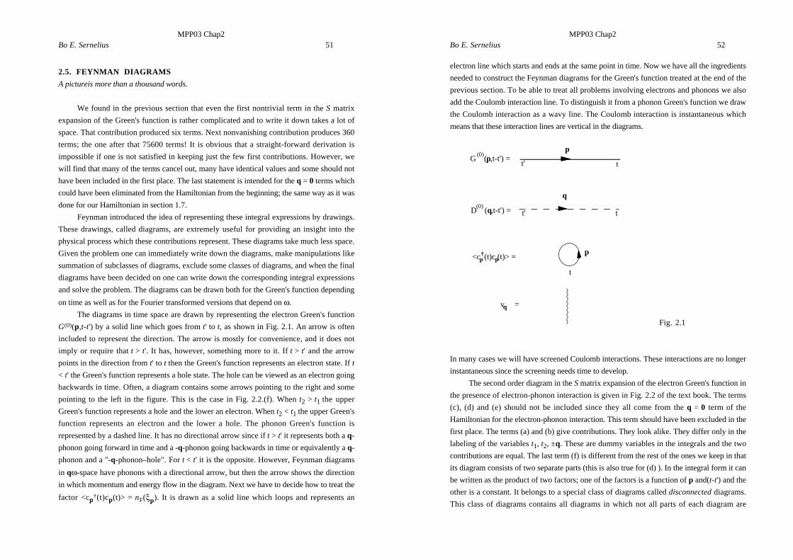
The diagrams in time space are drawn by representing the electron Green's function
G(0)(p,t-t') by a solid line which goes from t' to t, as shown in Fig. 2.1. An arrow is often
included to represent the direction. The arrow is mostly for convenience, and it does not
imply or require that t > t'. It has, however, something more to it. If t > t' and the arrow
points in the direction from t' to t then the Green's function represents an electron state. If t
< t' the Green's function represents a hole state. The hole can be viewed as an electron going
backwards in time. Often, a diagram contains some arrows pointing to the right and some
pointing to the left in the figure. This is the case in Fig. 2.2.(f). When t2 > t1 the upper
Green's function represents a hole and the lower an electron. When t2 < t1 the upper Green's
function represents an electron and the lower a hole. The phonon Green's function is
represented by a dashed line. It has no directional arrow since if t > t' it represents both a q-
phonon going forward in time and a -q-phonon going backwards in time or equivalently a q-
phonon and a "-q-phonon–hole". For t < t' it is the opposite. However, Feynman diagrams
in qw-space have phonons with a directional arrow, but then the arrow shows the direction
in which momentum and energy flow in the diagram. Next we have to decide how to treat the
factor <cp†(t)cp(t)> = nF(xp). It is drawn as a solid line which loops and represents an
MPP03 Chap2Bo E. Sernelius 52
electron line which starts and ends at the same point in time. Now we have all the ingredients
needed to construct the Feynman diagrams for the Green's function treated at the end of the
previous section. To be able to treat all problems involving electrons and phonons we also
add the Coulomb interaction line. To distinguish it from a phonon Green's function we draw
the Coulomb interaction as a wavy line. The Coulomb interaction is instantaneous which
means that these interaction lines are vertical in the diagrams.
p
t' tG (p,t-t') =
(0)
q
t' tD (q,t-t') =(0)
<c (t)c (t)> =p p† p
t
v =q
Fig. 2.1
In many cases we will have screened Coulomb interactions. These interactions are no longer
instantaneous since the screening needs time to develop.
The second order diagram in the S matrix expansion of the electron Green's function in
the presence of electron-phonon interaction is given in Fig. 2.2 of the text book. The terms
(c), (d) and (e) should not be included since they all come from the q = 0 term of the
Hamiltonian for the electron-phonon interaction. This term should have been excluded in the
first place. The terms (a) and (b) give contributions. They look alike. They differ only in the
labeling of the variables t1, t2, ±q. These are dummy variables in the integrals and the two
contributions are equal. The last term (f) is different from the rest of the ones we keep in that
its diagram consists of two separate parts (this is also true for (d) ). In the integral form it can
be written as the product of two factors; one of the factors is a function of p and(t-t') and the
other is a constant. It belongs to a special class of diagrams called disconnected diagrams.
This class of diagrams contains all diagrams in which not all parts of each diagram are
MPP03 Chap2Bo E. Sernelius 53
connected. We will come back to these diagrams in next section.
2.6. VACUUM POLARIZATION GRAPHS
We now turn our attention to the factor which to this point we have been ignoring:
0 0
01 0 1 0S
i
nd t d t TV t V t
n
nn n( , )
!ˆ( ) ˆ( ) .• -• =
-( )=
•
-•
•
-•
•Â Ú Úh
L L
This should have been in the denominator of the Green's function. Each term in this
expansion generates a series of terms. Each of these terms are constants. These generated
Feynman diagrams are called vacuum polarization graphs. If we were to determine this
quantity to second order with electron-phonon interaction as V we would get a 1 from the
zeroth order, no contribution from first order and two diagrams from the second order
contribution. These two diagrams are exactly the two disconnected parts of the diagrams in
Fig. 2.2 (d) and (e). If we were to write down all diagrams from the expansion of the
numerator of the Green's function, pick out one particular connected diagram, scan through
all disconnected diagrams and pick out all of these that have the same connected part as the
one we have chosen we would find the following: The disconnected parts of all the diagrams
we have picked out generates exactly the vacuum polarization graphs. This is true for every
choice of connected diagram. Thus the numerator of the Green's function can be written as a
product of two factors; one containing all connected diagrams; one containing all vacuum
polarization graphs. The last factor cancels exactly the denominator of the Green's function.
Thus in the expansion of the Green's function we should proceed as before and expand the
numerator and from this expansion discard all disconnected diagrams.Thus,
iG t ti
nd t d t
Tc t V t V t V t c t
s
n
nn
s n s
( , ' )( )
!
ˆ ( ) ˆ( ) ˆ( ) ˆ( ) ˆ ( ' ) ., ,†
p
p p
- = -
¥=
-•
•
-•
•Â Ú ÚhL
L
01
0 1 2 0
(connected)
Next we get rid of the 1/n! factor. It turns out to be just n! terms exactly alike in each bracket
of the nth term in the expansion. Thus if we consider only different terms, we obtain the
result
iG t t i d t d t
Tc t V t V t V t c t
sn
nn
s n s
( , ' ) ( )
ˆ ( ) ˆ( ) ˆ( ) ˆ( ) ˆ ( ' ) . ( ), ,†
p
p p
- = -
¥
=-•
•
-•
•Â Ú Úh L
L
01
0 1 2 0different connected
(2.6.3)
MPP03 Chap2Bo E. Sernelius 54
Let us now take the Fourier transform of this expression with respect to (t-t') for the case we
have studied. First we rewrite our obtained expression after all noncontributing terms have
been discarded. The result is
iG t t iG t t i d t d t
vM iD t t iG t t iG t t iG t t
s s
s s s
( , ' ) ( , ' )
( , ) ( , ) ( , ) ( , ' )
( )
( ) ( ) ( ) ( )
p p
q p p q pqq
- = - + -( )
¥ - - - - -(È
ÎÍÍ
˘
˚˙˙
-•
•
-•
•Ú Ú
Â
0 21 2
2 01 2
01
01 2
02
1
h
Now we take the inverse Fourier transform of the phonon Green's function
D t td
e Di t t( ) ' ( ) ( )( , )'
( , ' ) ,01 2
0
21 2q q- = - -
-•
•Ú w
pww
insert this and take the Fourier transform of the whole expression. The final result is
G G G
id
vM D G
s s s s
s s
( , ) ( , ) ( , ) ( , ) ;
( , )'
( , ' ) ( , ' ) ,
( ) ( ) ( )
( ) ( ) ( )
p p p p
p q p qqq
w w w w
w wp
w w w
= + [ ]= ( ) - -
È
ÎÍÍ
˘
˚˙˙-•
•Ú Â
0 0 2 1
1 2 2 0 012
1
S
S h
where Ss(1) is the self-energy due to one-phonon processes. We notice that the Green's
function inside the self-energy has the same spin index as the Green's function we are
studying. This is true in most cases. If on the other hand the interaction can flip spins then
the self energy will have to have two spin indices. This is also true for the interacting
Green's function. In that case the Green's functions and selfenergies are matrices and all
products of two functions are really matrix products. However, we will not consider this
case here.

MPP03 Chap2Bo E. Sernelius 55
2.7. DYSON'S EQUATION
If we sum the series of terms to infinite order we find that all higher order terms have
an unperturbed Green's function at both ends of the diagram. This means that we can write
G G G Gs s s s s( , ) ( , ) ( , ) ( , ) ( , ) ,( ) ( ) ( )p p p p pw w w w w= +0 0 0S
where Ss is the self-energy.
Now, we need to introduce some new concepts:
1. A self-energy insertion is defined as any part of a diagram that is connected to the rest of
the diagram by two particle lines(one in and one out).
2. A proper self-energy insertion is a self-energy insertion, which cannot be separated into
two pieces by cutting a single particle line.
3. The proper self-energy is the sum of all proper self-energy insertions. It is denoted by
Ss*.
It follows from these definitions that the self-energy consists of a sum of all possible
repetitions of the proper self-energy, i.e.
S S S S
S S Ss s s s s
s s s s s
G
G G
( , ) ( , ) ( , ) ( , ) ( , )
( , ) ( , ) ( , ) ( , ) ( , ) .
* * ( ) *
* ( ) * ( ) *
p p p p p
p p p p p
w w w w w
w w w w w
= +
+ +
0
0 0 L
This can be written as
S S S Ss s s s sG( , ) ( , ) ( , ) ( , ) ( , ) ,* * ( )p p p p pw w w w w= + 0
and be solved to give
S SSs
s
s sG( , )
( , )
( , ) ( , ).
*
* ( )pp
p pw w
w w=
-1 0
This is the Dyson's equation for the self-energy.
Putting this into the expression for the Green's function gives
MPP03 Chap2Bo E. Sernelius 56
G G G G
GG G
G
s s s s s
ss s s
s s
( , ) ( , ) ( , ) ( , ) ( , )
( , )( , ) ( , ) ( , )
( , ) ( , );
( ) ( ) ( )
( )( ) * ( )
* ( )
p p p p p
pp p p
p p
w w w w w
w w w ww w
= +
= +-
0 0 0
00 0
01
S
SS
GG
Gs
s
s s
( , )( , )
( , ) ( , )
( )
* ( )pp
p pw w
w w=
-
0
01 S
The relation in the box is the Dyson's equation for the electron Green's function. The
electron self-energy is sometimes called a mass operator.
The Green's function in the example with the degenerate electron gas becomes
Gn
i
n
iF F
ss
s s
s
s sw
xw x d w
xw x d w
( , )( )
/ ( , )
( )
/ ( , ),
,*
,
,*k
k kk
k
k
k=
- - -+
-- + -h hS S
1
The self-energy has real and imaginary parts. We shall show later that the imaginary part
changes sign at w = 0. It is positive for negative w and negative for positive w.
For phonons we have
DD
D( , )
( , )
( , ) ( , ).
( )
q qw w
p w w=
-
0
01
This is the Dyson's equation for the phonon Green's function. The phonon self-energy is
sometimes called a polarization operator.
The phonon Green's function at zero temperature can be written as
Di
( , )( , )
q
q qw
ww w d w p w
=- + -
2
22 2
The real and imaginary parts of the self-energies each have interpretations. The
imaginary part of the self-energies is interpreted as causing the damping of the particle
motion. They are related to the finite mean free path of the excitation or its energy and
momentum uncertainty. The real parts are actual energy shifts of the excitation, which may
also change its dynamical motion. The excitation may alter its effective mass or group
velocity because of the self-energy contributions. It is actually hS* and hP* that have
dimension energy and are the actual self-energies.
MPP03 Chap2Bo E. Sernelius 57
2.8. RULES FOR CONSTRUCTING DIAGRAMS
1. Draw the Feynman diagram for the self-energy term, with all phonon, Coulomb,
and electron lines.
2. For each electron line, introduce the following Green's function:
Gn
i
n
iF F
ab aba
a
a
aw d
xw x d
xw x d
( ) ,
,
,
,( , )
( )
/
( )
/0 1
p p
p
p
p=
- -+
-- +
È
ÎÍÍ
˘
˚˙˙h h
The da b indicates that the electron line must have the same spin at both ends of the
propagator line. This feature is important in spin problems. The Green's function is valid for
a degenerate Fermi system, but can also be used for the empty band case if the chemical
potential is assumed to be at the bottom of the band.
3. For each phonon line, introduce the following phonon propagator:
Di
( )( , ) .02 2
2q q
qw
ww w d
=- +
Also add a factor |Mq|2/h for each phonon Green's function, where Mq is the matrix element
for electron-phonon interaction.
4. Add a Coulomb potential vq = 4pe2/q2 for each Coulomb interaction. Note that we
always draw the Coulomb line as a wiggly vertical line. The Coulomb interaction is regarded
as happening instantaneously in time, and time flows horizontally, from left to right, in our
diagrams. One could, of course, have time flow upwards and draw the Coulomb interactions
as horizontal wiggly lines.
5. Conserve energy and momentum at each vertex. Thus each electron line, phonon
line, and Coulomb line have their variables labeled to conform with this rule.
6. Sum over internal degrees of freedom: momentum, frequency, and spin. The
summation over momentum and frequency and spin should be performed according to
12
2 2
3
3
v
d
d d
wp
pwp
s
s
-•
•
-•
•
ÚÂ
Ú ÚÂ
ÏÌÓ
( )
q
q
,
,
,
for box normalization
and discrete momentum summations
for integration over momentum
If one is calculating a self-energy term S(p,w), then all momentum and frequencies except p
and w are internal and must be summed over.
MPP03 Chap2Bo E. Sernelius 58
7. Finally, we multiply the result by the factor (i/h)m(-1)F where F is the number of
closed fermion loops. The index m is chosen as follows:
a. For electron self-energies, m is the number of internal phonon and Coulomb
lines.
b. For phonon self-energies, m is one-half the number of vertices.
8. For each photon line which interacts with particles through the j.A interaction,
insert a factor
e
mD
hÊË
ˆ¯ +( ) +( )Â
2
2 2k q q k q/ ( , ) ' /m mnmn
nw
where Dmn(q,w) is the photon Green's function and k and k' are the wave vectors of
particles scattered at the two vertices. The other possible interaction of a charged particle with
photons occurs through the term
e
mcA r
e
mA Ai
2
22
2
2 2( ) ( ) ( ) ( )
, ,
= -Â r mm
mq k q kq k
We will later see that this interaction contributes a self-energy term of e2n0/m to the self-
energy of the photon, where n0 is the density of charged particles.
To obtain more general rules for constructing and interpreting Feynman diagrams we
have to distribute the (i/h)m factor in the diagrams. To do this we attach the factor (i/h)1/2 at
each vertex(this can be done slightly more general. If we have a situation where the system
consists of particles of different charge then the vertex factor should be multiplied by the
valence Z for the particle scattered at the vertex). Then each diagram consists of only Green's
functions (for particles, phonons or photons) and vertices. The Coulomb interaction line can
be viewed as a photon Green's function. The Coulomb interaction between two particles can
be regarded as the interchange of two different types of photons. The Coulomb interaction
has a Dyson's equation
vv
v P
v
q
q
q
q
( )( , )
( , ),
*ww
e w
=-
=
1
where P* is the proper self-energy for the Coulomb interaction or the polarization operator.

MPP03 Chap2Bo E. Sernelius 59
If only the lowest order contribution of P* is kept the result is co, the susceptibility
introduced at the end of chapter 1. With this choice the dielectric function is the RPA
dielectric function. The Coulomb interaction is now screened and no longer instantaneous.
Let us study the following part of a Feynman diagram:
(k+q,w'+w)
vq
vq
(i/h)1/2
(k,w')
(i/h)1/2
The "bubble" including the two vertices is just co, and the diagram is interpreted as
v v
i
v
dG Gq q
k
q k k q20
2 0 012
c w wp
w w ws
s s( , )( ) '
( , ' ) ( , ' ) ,,
( ) ( )= - + +-•
•
ÚÂh
where the minus sign comes from the fact that co contains one closed fermion loop. If we
now have a diagram with phonon lines instead of Coulomb interaction lines we get
(i) 1/2(M(-q)/h)(i)1/2(M(q)/h)
D (q,w)(0)
D (q,w)(0)
(k+q,w'+ w)
(k,w')
The diagram is interpreted as
D D
M q( ) ( ) ( )( , ) ( , ) ( , )( )
( , ) ,0 2 1 0 22
0q q q qw p w w c w=h
MPP03 Chap2Bo E. Sernelius 60
where p(1)(q,w) is the lowest order phonon self-energy insertion. Now, let us study another
diagram
(p,w')
(p-q,w'-w)
(p'+q
,w''+
w)(p',w'')
(q,w)vq
(i/h)1/2
(i/h)1/2
This describes the scattering of two particles, electrons say, against each other via the
Coulomb interaction. The electron-phonon interaction gives rise to a very similar diagram,
viz.
(p,w')
(p-q,w'-w)
(p'+q
,w''+
w)(p',w'')
D
(q,w
)(0
)
(i)1/
2(M
(q)/
h)(i)
1/2
(M(-
q)/h
)
This leads to an effective electron-electron interaction contribution. Together these
contributions give
˜( , )
( )( , ) .( )v v
M qDq qqw w= +
20
h

MPP03 Chap2Bo E. Sernelius 61
Let us see what we get for the polar semiconductor that we treated in of chapter 1. We find
˜( , )( )
( , )
( )
( )
( ),
( )vv g q
D
v e
q i
v e
q i
v
LOLO
LO
LO
LO
q qq
q
q
q
we
w
ep e e
e ew w
w w d
ep e e
e ew
w w d
e w
= +
= + -ÊËÁ
ˆ¯̃ - +
= + -- +
=
•
•
•
•
•
•
•
20
2
20
02 2
2
20
0
2
2 2
2 2
4
h
hh
where e(w) is the frequency dependent background dielectric function which results from the
combined screening by the valence electrons (virtual transitions across the band gap) and the
phonons. This dielectric function is
e we w w
w ee
w d
e w ww w w d w w d
e ee e
w
( )
;
( )
( ) .
=-( )
- +
=-( )
- +-
+ -È
ÎÍ
˘
˚˙
=• =
•
•
•
•
2 2
2
0
2
2 2
0
2
21 1
0
LO
LO
LO
TO TO TO
TO
i
i i
124 34
This dielectric function vanishes at the longitudinal phonon frequency and has a delta
function imaginary part at the transverse phonon frequency.
The building blocks we have at our disposal when drawing the electron Green's function
diagrams, when the interaction is the electron-phonon interaction, are
MPP03 Chap2Bo E. Sernelius 62
e-ph
2nd order
and
4th order
e-ph
The corresponding building blocks in the case of electron-electron interaction are

MPP03 Chap2Bo E. Sernelius 63
e-e
1st order
and
2nd order
e-e
The resulting 1st (2nd) order diagrams in the electron-electron interaction case look exactly
the same as the 2nd (4th) order diagrams in the electron-phonon interaction case except for
that the interaction line is now wiggly instead of dashed.
MPP03 Chap2Bo E. Sernelius 64
2.9. TIME-LOOP S MATRIX
A. Six Green's Functions.
We will discuss six different Green's functions. The type we have introduced so far is
called the time-ordered version. The other five are the anti-time-ordered (denoted by a bar
over the t), "G less" G<, "G larger" G>, the retarded Gret , and the advanced Gadv . For
fermions the six Green's functions are defined as
G t i c t c
G t i c c t
G t t G t t G t
G t t G t t G t
G t
t
t
ret
>
<
> <
< >
= -
=
= + -[ ]= + -[ ]
( , ) ( ) ( )
( , ) ( ) ( )
( , ) ( ) ( , ) ( ) ( , )
( , ) ( ) ( , ) ( ) ( , )
( ,
†
†
k
k
k k k
k k k
k
k k
k k
0
0
1
1
q q
q q
)) ( ) ( , ) ( , ) ( ) ( ), ( )
( , ) ( ) ( , ) ( , ) .
†= -[ ] = - { }= -[ ] -[ ]
> <
< >
q q
q
t G t G t i t c t c
G t t G t G tadv
k k
k k k
k k 0
1
We see that the time-ordered Green's function is equal to G> for positive t and G< for
negative. The retarded Green's function is zero for negative t. For positive t it is equal to G>
- G<. The advanced function is zero for positive t. For negative t it is equal to G< - G>. The
unperturbed fermion Green's functions are
G t i t n t n e
G t i t n t n e
G t in e
G t
ti t
ti t
i t
( ) /
( ) /
/
( , ) ( ) ( )
( , ) ( ) ( )
( , )
( , )
0
0
0
0
1 1
1 1
k
k
k
k
k k
k k
k
k
k
k
= - -[ ] - -[ ]{ }= - -[ ] -[ ] -{ }=
= -
-
-
< -
>
q q
q q
x
x
x
h
h
h
ii n e
G t i t n t n e i t e
G t i t n t n e
i t
reti t i t
advi
1
1
1 1 1
0
0
-[ ]= - -[ ] +{ } = -
= - - -[ ] -[ ] - -[ ]{ }
-
- -
-
k
k k
k k
k
k k
k
k
k
x
x x
x
q q q
q q
/
( ) / /
( )
( , ) ( ) ( ) ( )
( , ) ( ) ( )
h
h h
tt i ti t e/ /( ) .h h= -[ ] -1 q xk
After Fourier transformation with respect to t, where an infinitesimal d has been added to the
frequency exponent to guarantee convergence in the ± • limits of the time integrals we obtain
MPP03 Chap2Bo E. Sernelius 65
Gn
i
n
i
Gn
i
n
i
G in
G i n
t
t
( )
( )
( , )/ /
( , )/ /
( , ) ( / )
( , )
0
0
0
0
1
1
2
1
k
k
k
k
k
k
k
k
k
k
k
k
k k
k
ww x d w x d
ww x d w x d
w p d w x
w
=- -
+ -- +
= - -- -
+- +
È
ÎÍ
˘
˚˙
= -
= - -[
<
>
h h
h h
h
]] -
=- +
+ -- +
=- +
=- -
+ -- -
=- -
2
1 1
1 1
0
0
p d w x
ww x d w x d w x d
ww x d w x d w x d
( / )
( , )/ / /
( , )/ / /
.
( )
( )
k
k
k
k
k k
k
k
k
k k
k
k
h
h h h
h h h
Gn
i
n
i i
Gn
i
n
i i
ret
adv
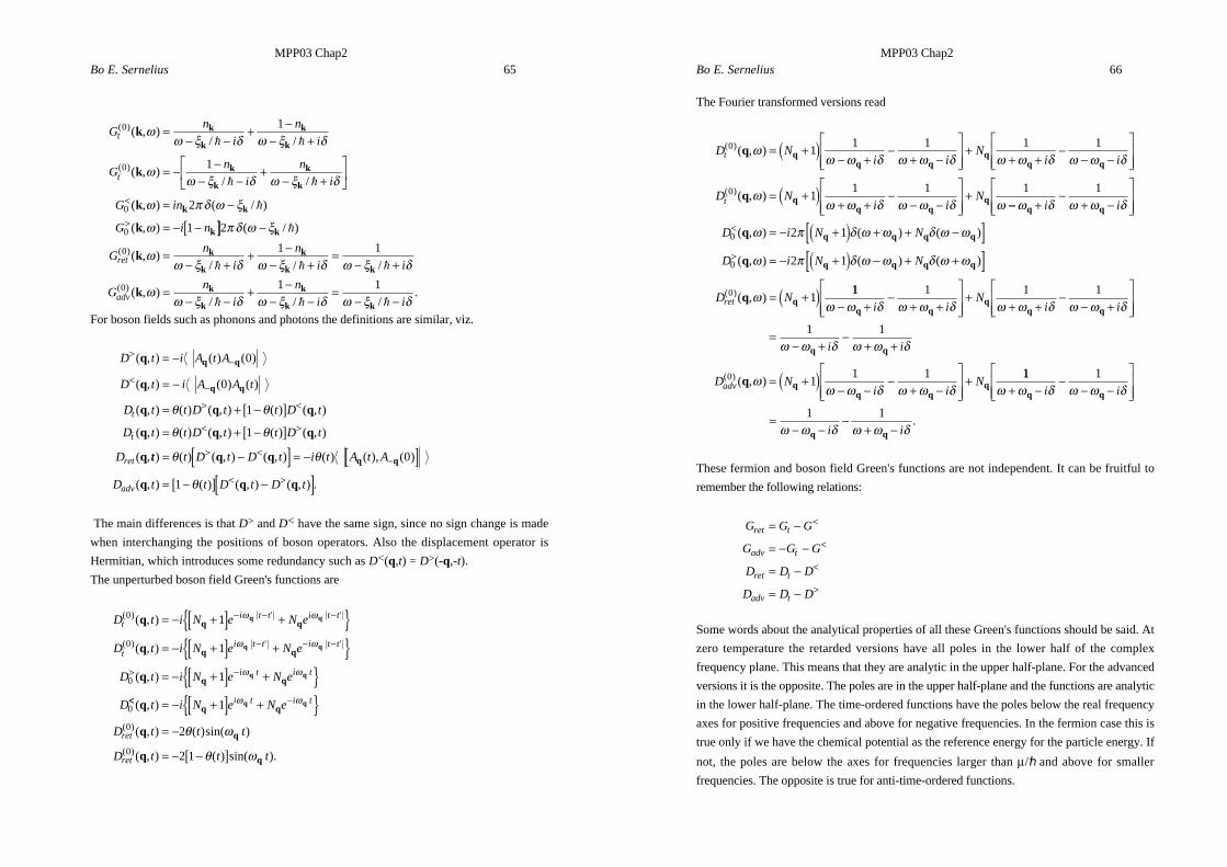
For boson fields such as phonons and photons the definitions are similar, viz.
D t i A t A
D t i A A t
D t t D t t D t
D t t D t t D t
D
t
t
ret
>-
<-
> <
< >
= -
= -
= + -[ ]= + -[ ]
( , ) ( ) ( )
( , ) ( ) ( )
( , ) ( ) ( , ) ( ) ( , )
( , ) ( ) ( , ) ( ) ( , )
( ,
q
q
q q q
q q q
q
q q
q q
0
0
1
1
q q
q q
tt t D t D t i t A t A
D t t D t D tadv
) ( ) ( , ) ( , ) ( ) ( ), ( )
( , ) ( ) ( , ) ( , ) .
= -[ ] = - [ ]= -[ ] -[ ]
> <-
< >
q q
q
q q
q q q
q q 0
1
The main differences is that D> and D< have the same sign, since no sign change is made
when interchanging the positions of boson operators. Also the displacement operator is
Hermitian, which introduces some redundancy such as D<(q,t) = D>(-q,-t).
The unperturbed boson field Green's functions are
D t i N e N e
D t i N e N e
D t i N e N e
D
ti t t i t t
ti t t i t t
i t i t
( ) ' '
( ) ' '
( , )
( , )
( , )
0
0
0
0
1
1
1
q
q
q
q q
q q
q q
q q
q q
q q
= - +[ ] +{ }= - +[ ] +{ }= - +[ ] +{ }
- - -
- - -
> -
w w
w w
w w
<< -= - +[ ] +{ }= -
= - -[ ]
( , )
( , ) ( )sin( )
( , ) ( ) sin( ).
( )
( )
q
q
q
q q
q
q
q qt i N e N e
D t t t
D t t t
i t i t
ret
ret
1
2
2 1
0
0
w w
q w
q w
MPP03 Chap2Bo E. Sernelius 66
The Fourier transformed versions read
D Ni i
Ni i
D Ni i
N
t
t
( )
( )
( , )
( , )
0
0
11 1 1 1
11 1 1
q
q
qq q
qq q
qq q
q
ww w d w w d w w d w w d
ww w d w w d w
= +( ) - +-
+ -È
ÎÍÍ
˘
˚˙˙
++ +
-- -
È
ÎÍÍ
˘
˚˙˙
= +( ) + +-
- -È
ÎÍÍ
˘
˚˙˙
+-- +
-+ -
È
ÎÍÍ
˘
˚˙˙
= - +( ) + + -[ ]= - +( ) - + +[ ]= +( )
<
>
w d w w d
w p d w w d w w
w p d w w d w w
w
q q
q q q q
q q q q
q
q
q
q
i i
D i N N
D i N N
D Nret
1
2 1
2 1
1
0
0
0
( , ) ( ) ( )
( , ) ( ) ( )
( , )( ) 11 1 1 1
1 1
11 10
w w d w w d w w d w w d
w w d w w d
ww w d w w d
- +-
+ +È
ÎÍÍ
˘
˚˙˙
++ +
-- +
È
ÎÍÍ
˘
˚˙˙
=- +
-+ +
= +( ) - --
+ -È
ÎÍÍ
˘
˚˙˙
+
q qq
q q
q q
qq q
i iN
i i
i i
D Ni i
Nadv( ) ( , )
11 1
1 1
w w d w w d
w w d w w d
+ --
- -È
ÎÍÍ
˘
˚˙˙
=- -
-+ -
q q
q q
i i
i i.
These fermion and boson field Green's functions are not independent. It can be fruitful to
remember the following relations:
G G G
G G G
D D D
D D D
ret t
adv t
ret t
adv t
= -
= - -
= -
= -
<
<
<
>
Some words about the analytical properties of all these Green's functions should be said. At
zero temperature the retarded versions have all poles in the lower half of the complex
frequency plane. This means that they are analytic in the upper half-plane. For the advanced
versions it is the opposite. The poles are in the upper half-plane and the functions are analytic
in the lower half-plane. The time-ordered functions have the poles below the real frequency
axes for positive frequencies and above for negative frequencies. In the fermion case this is
true only if we have the chemical potential as the reference energy for the particle energy. If
not, the poles are below the axes for frequencies larger than m/h and above for smaller
frequencies. The opposite is true for anti-time-ordered functions.
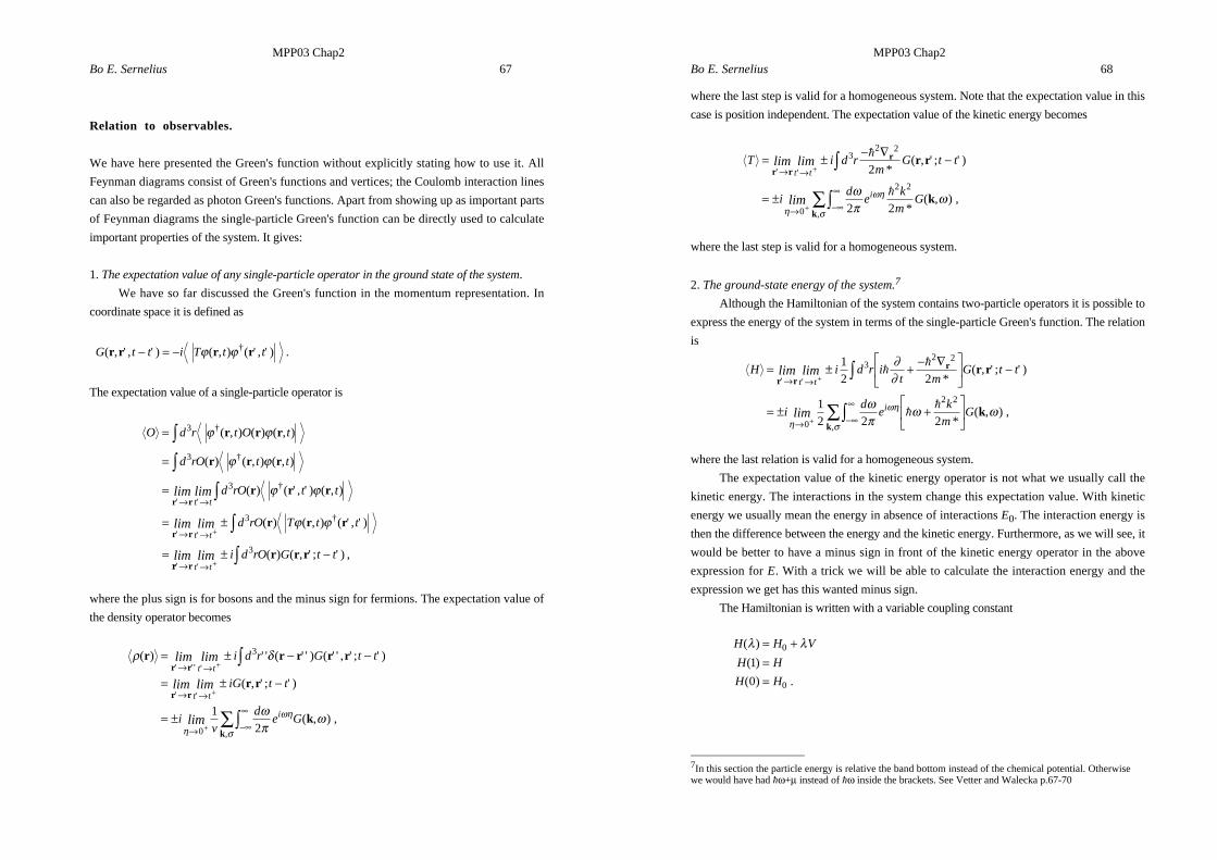
MPP03 Chap2Bo E. Sernelius 67
Relation to observables.
We have here presented the Green's function without explicitly stating how to use it. All
Feynman diagrams consist of Green's functions and vertices; the Coulomb interaction lines
can also be regarded as photon Green's functions. Apart from showing up as important parts
of Feynman diagrams the single-particle Green's function can be directly used to calculate
important properties of the system. It gives:
1. The expectation value of any single-particle operator in the ground state of the system.
We have so far discussed the Green's function in the momentum representation. In
coordinate space it is defined as
G t t i T t t( , ' , ' ) ( , ) ( ' , ' ) .†r r r r- = - j j
The expectation value of a single-particle operator is
O d r t O t
d rO t t
d rO t t
d rO T t t
t
t
=
=
=
= ±
=
ÚÚ
Ú
ÚÆ Æ
Æ Æ +
3
3
3
3
j j
j j
j j
j j
†
†
' '
†
' '
†
( , ) ( ) ( , )
( ) ( , ) ( , )
( ) ( ' , ' ) ( , )
( ) ( , ) ( ' , ' )
r r r
r r r
r r r
r r r
r r
r r
lim lim
lim lim
t
t
rr rr r r
' '( ) ( , ' ; ' ) ,
Æ Æ +± -Úlim lim
t ti d rO G t t3
where the plus sign is for bosons and the minus sign for fermions. The expectation value of
the density operator becomes
r d
wp
wh
wh
s
( ) ' ' ( ' ' ) ( ' ' , ' ; ' )
( , ' ; ' )
( , ) ,
' ' ' '
' '
,
r r r r r
r r
k
r r
r r
k
= ± - -
= ± -
= ±
Æ Æ
Æ Æ
Æ -•
•
+
+
+
Ú
ÚÂ
lim lim
lim lim
lim
t
t
t
t
i
i d r G t t
iG t t
iv
de G
3
0
12
MPP03 Chap2Bo E. Sernelius 68
where the last step is valid for a homogeneous system. Note that the expectation value in this
case is position independent. The expectation value of the kinetic energy becomes
T i d rm
G t t
id
ek
mG
t
i
= ± - — -
= ±
Æ Æ
Æ -•
•
+
+
Ú
ÚÂ
r r
r
k
r r
k
' '
,
*( , ' ; ' )
*( , ) ,
lim lim
lim
t
32 2
0
2 2
2
2 2
h
h
h
wh
s
wp
w
where the last step is valid for a homogeneous system.
2. The ground-state energy of the system.7
Although the Hamiltonian of the system contains two-particle operators it is possible to
express the energy of the system in terms of the single-particle Green's function. The relation
is
H i d r it m
G t t
id
ek
mG
t
i
= ± + - —È
ÎÍ
˘
˚˙ -
= ± +È
ÎÍ
˘
˚˙
Æ Æ
Æ -•
•
+
+
Ú
ÚÂ
r r
r
k
r r
k
' '
,
*( , ' ; ' )
*( , ) ,
lim lim
lim
t
12 2
12 2 2
32 2
0
2 2
hh
hh
∂∂
wp
w wh
wh
s
where the last relation is valid for a homogeneous system.
The expectation value of the kinetic energy operator is not what we usually call the
kinetic energy. The interactions in the system change this expectation value. With kinetic
energy we usually mean the energy in absence of interactions E0. The interaction energy is
then the difference between the energy and the kinetic energy. Furthermore, as we will see, it
would be better to have a minus sign in front of the kinetic energy operator in the above
expression for E. With a trick we will be able to calculate the interaction energy and the
expression we get has this wanted minus sign.
The Hamiltonian is written with a variable coupling constant
H H V
H H
H H
( )
( )
( ) .
l l= +==
0
0
1
0
7In this section the particle energy is relative the band bottom instead of the chemical potential. Otherwisewe would have had hw+m instead of hw inside the brackets. See Vetter and Walecka p.67-70

MPP03 Chap2Bo E. Sernelius 69
Let,
H E
E H
( ) ( ) ( ) ( )
( ) ( )
( ) ( ) ( ) ( ) .
l l l l
l l
l l l l
Y Y
Y Y
Y Y
0 0
0 0
0 0
1
=
=
fl
=
The derivative with respect to the coupling constant reduces to
d
dE
d
dH H
d
d
dH
d
Ed
dV
V
ll l
ll l l l l
ll l
ll
ll
l l l l
l l
( )( )
( ) ( ) ( ) ( )( )
( )( )
( )
( ) ( ) ( ) ( ) ( )
( ) ( ) .
= + +
= +
=
Y Y Y Y Y Y
Y Y Y Y
Y Y
00 0
00 0
0 0 0 0
0 0
Integrate this equation with respect to the coupling constant from 0 to 1
E Ed
V- = Ú0 0
10 0
ll
l l lY Y( ) ( ) .
The shift in the ground-state energy is expressed solely in terms of the matrix element of the
interaction lV.
E Ed
H T
id d
ek
mGi
- = -
= ± -È
ÎÍ
˘
˚˙
Ú
Ú ÚÂÆ -•
•
+
0 0
10 0
0 0
1 2 212 2 2
ll
l l l
ll
wp
w wh
wh l
s
Y Y( ) ( ) ( )
*( , ) .
,lim h
hk
k
MPP03 Chap2Bo E. Sernelius 70
Using Dyson's equation for the Green's function leads to
E E id d
e G
id d
e G
i
i
- = ± +[ ]= ±
Æ -•
•
Æ -•
•
+
+
Ú ÚÂ
Ú ÚÂ
00 0
1
0 0
1
12 2
1
12 2
h
wh l l
s
h
wh l l
s
ll
wp
w w
ll
wp
w w
lim
lim
h
h
S
S
*
,
*
,
( , ) ( , )
( , ) ( , ) .
k k
k k
k
k
The integration over the "1" term on the first line vanishes in the proper limit. We have here
given one way to derive the interaction energy of the system. This formulation is useful since
the result is given in terms of the proper self-energy and Green's function – quantities that
we know how to calculate. We will use an alternative method in the second part of this
course.
3. The excitation spectrum of the system.
The function G(k,w) has simple poles at the exact excitation energies of the interacting
system corresponding to a momentum hk.
Thus the single-particle Green's function gives us most of the information we need to
understand our interacting system. However there is one important thing missing. We don't
get the system's response to external perturbations. A recipe for calculating these things is
given by the Kubo formula:
Assume that an external field F(r,t) gives rise to a perturbing term in the Hamiltonian:
H d rA t F text = -Ú 3 ( , ) ( , ) .r r
The system responds with an induced density of some kind; it may, e.g., be a chargedensity, a current density or a spin density. For a homogeneous system in the linearresponse regime the induced quantity can be related to the external field by a susceptibility
function a(r,t) according to
B t d r dt t t F t
B F
ind
ind
( , ) ' ' ( ' , ' ) ( ' , ' )
( , ) ( , ) ( , ) ,
r r r r
q q q
= - -
=Ú Ú3 a
w a w w
where
a q( ' , ' ) ( ' ) ( , ), ( ' , ' ) .r r r r- - = - [ ]t t
it t B t A t
h
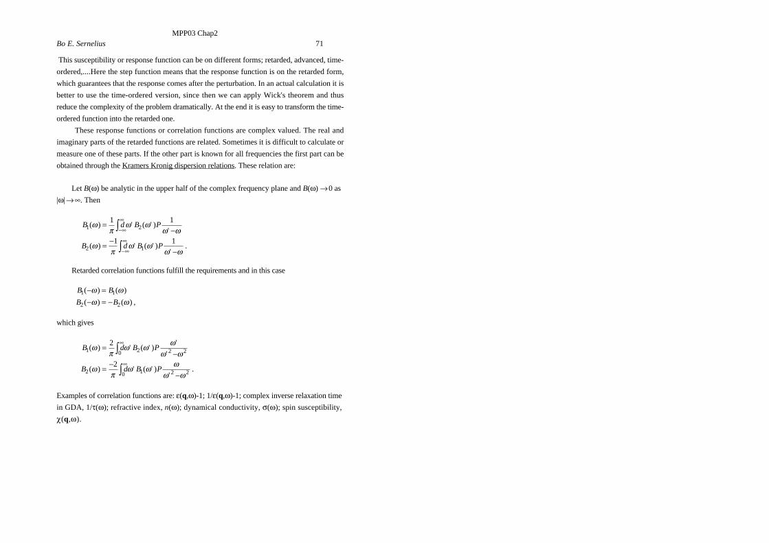
MPP03 Chap2Bo E. Sernelius 71
This susceptibility or response function can be on different forms; retarded, advanced, time-
ordered,....Here the step function means that the response function is on the retarded form,
which guarantees that the response comes after the perturbation. In an actual calculation it is
better to use the time-ordered version, since then we can apply Wick's theorem and thus
reduce the complexity of the problem dramatically. At the end it is easy to transform the time-
ordered function into the retarded one.
These response functions or correlation functions are complex valued. The real and
imaginary parts of the retarded functions are related. Sometimes it is difficult to calculate or
measure one of these parts. If the other part is known for all frequencies the first part can be
obtained through the Kramers Kronig dispersion relations. These relation are:
Let B(w) be analytic in the upper half of the complex frequency plane and B(w) Æ 0 as
|w| Æ •. Then
B d B P
B d B P
1 2
2 1
1 1
1 1
( ) ' ( ' )'
( ) ' ( ' )'
.
wp
w ww w
wp
w ww w
=-
= --
-•
•
-•
•
Ú
Ú
Retarded correlation functions fulfill the requirements and in this case
B B
B B1 1
2 2
( ) ( )
( ) ( ) ,
- =- = -
w ww w
which gives
B d B P
B d B P
1 0 2 2 2
2 0 1 2 2
2
2
( ) ' ( ' )'
'
( ) ' ( ' )'
.
wp
w w ww w
wp
w w ww w
=-
= --
•
•
Ú
Ú
Examples of correlation functions are: e(q,w)-1; 1/e(q,w)-1; complex inverse relaxation time
in GDA, 1/t(w); refractive index, n(w); dynamical conductivity, s(w); spin susceptibility,
c(q,w).