MPM: Joint Representation of Motion and Position Map for Cell Tracking

Junya Hayashida Kazuya Nishimura Ryoma BiseKyushu University, Fukuoka, Japan, {bise@ait.kyushu-u.ac.jp}

Abstract

Conventional cell tracking methods detect multiple cellsin each frame (detection) and then associate the detec-tion results in successive time-frames (association). Mostcell tracking methods perform the association task indepen-dently from the detection task. However, there is no guar-antee of preserving coherence between these tasks, and lackof coherence may adversely affect tracking performance. Inthis paper, we propose the Motion and Position Map (MPM)that jointly represents both detection and association for notonly migration but also cell division. It guarantees coher-ence such that if a cell is detected, the corresponding mo-tion flow can always be obtained. It is a simple but powerfulmethod for multi-object tracking in dense environments. Wecompared the proposed method with current tracking meth-ods under various conditions in real biological images andfound that it outperformed the state-of-the-art (+5.2% im-provement compared to the second-best).

1. IntroductionCell behavior analysis is an important research topic in

the fields of biology and medicine. Individual cells must bedetected and tracked in populations to analyze cell behav-ior metrics including cell migration speed and frequency ofcell division. However, it is too time consuming to man-ually track a large number of cells. Therefore, automaticcell tracking is required. Cell tracking in phase-contrast mi-croscopy is a challenging multi-object tracking task. This isbecause the cells tend to have very similar appearance andtheir shapes severely deform. Therefore, it is difficult toidentify the same cell among frames based on only its ap-pearance. Moreover, cells in contact with each other oftenhave blurry intercellular boundaries. In this case, it is diffi-cult to identify touching cells from only one image. Finally,a cell may divide into two cells (cell mitosis), which is avery different situation from that of general object tracking.

The tracking-by-detection method is the most populartracking paradigm because of the good quality of the de-tection algorithms that use convolutional neural networks(CNNs) for the detection step. These methods detect cellsin each frame and then associate the detection results among

the time-frames by maximizing the sum of associationscores of hypotheses, where the association step is oftenperformed independently from the detection step [21, 31, 8].They basically use hand-crafted association scores based onthe proximity and similarity in shape of cells, but the scoresonly evaluate the similarity of individual cells; i.e., they donot use the context of nearby cells. Moreover, the scoresdepend on the conditions of the time-lapse images, such asthe frame interval, cell type, and cell density.

On the other hand, the positional relationship of nearbycells is important to identify the association when the den-sity is high. Several methods have been proposed for usingcontext information [32, 17]. Hayashida et al. [17] pro-posed a cell motion field (CMF) that represents the cellassociation between successive frames in order to directlypredict cell motion (association) by using a CNN. This en-ables cell tracking at low frame rates. This method outper-formed the previous methods that use hand-crafted associ-ation scores. However, it still independently performs thedetection and association inference. This raises the possi-bility of incoherence between the two steps; e.g., although acell is detected, there is no response at the detected positionin the CMF, and this would affect the tracking performance.

Many applications use multi-task learning [16, 19, 11,45], i.e., learning multiple-related tasks. This method basi-cally has common layers express task-shared features andoutput branches that represent task-specific features. Multi-task learning improves the accuracy of the tasks comparedwith individual learning. However, it is not easy to preservethe coherence between the detection and association tasks inmulti-task learning. If we simply apply a branch network,there is no guarantee that the coherence between these taskswill be preserved: e.g., the network may detect a cell butnot produce a corresponding association for the cell, whichwould adversely affect tracking performance.

Unlike such multi-task learning methods, we propose theMotion and Position Map (MPM) that jointly representsboth detection and association for not only migration butalso cell division, as shown in Fig. 1, where the distri-bution of magnitudes of MPM indicates the cell-positionlikelihood map at frame t; the direction of the 3D vectorencoded on a pixel in MPM indicates the motion direction

1

arX

iv:2

002.

1074

9v2

[cs

.CV

] 2

6 Fe

b 20

20

Input imagesequence

EstimatedMPM

t

t-n

t SiameseNets

frame t

frame t-1

(c) Cell position likelihood map

(a)Input images andmanual annotations

(b) Motion and position map(MPM)

(d) Movement vectorsfor cell association

Cell position

Mapping magnitude of each vector

MPM

Stretching each vector to t-1

t-1

t

t-1

t

1

0

t-1

t

(e) Estimating MPM for all frame

(f) Tracking result

Trajectories made by MPM

Association(motion)

t-n

Figure 1. Overview of the proposed method. (a) Input images in two successive frames and manual annotations of cell positions in eachframe and their association. (b) Motion and position map (MPM) that jointly represents both detection and association. MPM encodes thefollowing two pieces of information: (c) a cell-position likelihood map, which is a magnitude map of MPM. The peaks of this map indicatethe cells’ positions; (d) motion vector for a cell from t to t − 1. (e) Estimating the MPM for all frames by using siamese MPM-Nets. (f)The overall tracking results when using MPM.

from the pixel at t to the cell centroid at t− 1. Since MPMrepresents both detection and association, it guarantees co-herence; i.e., if a cell is detected, an association of the cellis always produced. In addition, we can obtain the cell po-sitions and their association for all frames by using siameseMPM networks, as shown in Fig. 1(e). Accordingly, even avery simple tracking method can be used to construct over-all cell trajectories with high accuracy (Fig. 1(f)). In theexperiments, our method outperformed the state-of-the-artsunder various conditions in real biological images.

Our main contributions are summarized as follows:

• We propose the motion and position map (MPM) thatjointly represents detection and association for notonly migration but also cell division. It guarantees co-herence such that if a cell is detected, the correspond-ing motion flow can always be obtained. It is a simplebut powerful method for multi-object tracking in denseenvironments.

• By applying MPM-Net to the entire image sequence,we can obtain the detection and association informa-tion for the entire sequence. By using the estimationresults, we can easily obtain the overall cell trajecto-ries without any complex process.

2. Related workCell tracking: Cell tracking methods can be roughly clas-sified into two groups: those with model-based evolutionand those based on detection-and-association. The first

group uses sequential Bayesian filters such as particle fil-ters [30, 38], or active contour models [24, 40, 43, 46]. Theyupdate a probability map or energy function of cell regionsby using the tracking results of the previous frame as theinitial state for the updates. These methods work well ifcells are sparsely distributed. However, these methods mayget confused when cells are close together with blurry inter-cellular boundaries or move over a long distance.

The second group of cell-tracking methods are based ondetection and association: first they detect cells in eachframe; then they determine associations between succes-sive frames. Many cell detection/segmentation methodshave been proposed to detect individual cells, by usinglevel set [25], watershed [28], graph-cut [4], optimizationusing intensity features [7], physics-based-restoration [44,39, 23], weakly-supervised [29] and CNN-based detectionmethods [33, 34, 1, 27, 3]. Moreover, many optimiza-tion methods have been proposed to associate the detectedcells. They maximize an association score function, in-cluding linear programming for frame-by-frame associa-tion [21, 5, 6, 46, 42] and graph-based optimization forglobal data association [8, 36, 39, 15]. These methods ba-sically use the proximity and shape similarity of cells formaking hand-crafted association scores. These associationscores depend on the cell culture conditions, such as theframe interval, cell types and cell density. In addition, thescores only evaluate the similarity of individual cells, notthe context of nearby cells. On the other hand, a human ex-pert empirically uses the positional relationship of nearby

2

cells in dense cases. Several methods have been proposedon how to use such context information [32, 17, 33]. Payeret al. [32] proposed a recurrent stacked hourglass network(ConvGRU) that not only extracts local features, but alsomemorizes inter-frame information. However, this methodrequires annotations for all cell regions as training data, andit does not perform well when the cells are small. Hayashidaet al. [17] proposed a cell motion field that represents thecell association between successive frames that can be esti-mated with a CNN. Their method is a point-level tracking,and thus it dramatically reduces annotation costs comparedwith pixel-level cell boundary annotation. These methodshave been shown to outperform those that use hand-craftedassociation scores. However, the method still performs thedetection and association inference independently. Thiscauses incoherence between steps, which in turn affectstracking performance.

Object tracking for general object: For single-objecttracking that finds the bounding box corresponding to giveninitial template, Siamese networks have been often usedto estimate the similarity of semantic features between thetemplate and target images [20, 22]. To obtain a good sim-ilarity map, this approach is based on representation learn-ing. However, in the cell tracking problem, there may bemany cells that have similar appearances; thus, the simi-larity map would have a low confidence level. Tracking-by-detection (detection-and-association) is also a standardapproach in multi-object tracking (MOT) for general ob-jects. In the association step, features of objects and mo-tion predictions [26, 12] are used to compute a similar-ity/distance score between pairs of detection and/or track-lets. Re-identification is often used for feature represen-tation [14, 2]. This method does not use the global spa-tial context, and the detection and association processes areseparated. Optimization techniques [41, 35] have been pro-posed for jointly performing the detection and associationprocesses; they jointly find the optimal solution of detectionand association from a candidate set of detections and asso-ciations. Sun et al. [37] proposed the Deep Affinity Net-work (DAN). Although this method jointly learns a featurerepresentation for identification and association, the detec-tion step is independent of these learnings.

Multi-task learning: Multi task learning (MTL) has beenwidely used in computer vision for learning similar taskssuch as pose estimation and action recognition [16]; depthprediction and semantic classification [19, 11]; and forroom floor plans [45]. Most multi-task learning network ar-chitectures for computer vision are based on existing CNNarchitectures [19, 9, 18]. These architectures basically havecommon layers and output branches that express both task-shared and task-specific features. For example, cross-stitchnetworks [19] contain one standard CNN per task, withcross-stitch units to allow features to be shared across tasks.

Such architectures require a large number of network pa-rameters and scale linearly with the number of tasks. In ad-dition, there is no guarantee of coherence among the tasksif we simply apply the network architecture to a multi-taskproblem such as detection and association. This means thatwe need to design a new loss function or architecture topreserve the coherence depending on the pairs of the tasks.To the best of our knowledge, multi-task learning methodsspecific to our problem have not been proposed.

Unlike these methods, we propose MPM for jointly rep-resenting the detection and association tasks at once. TheMPM can be estimated using simple U-net architecture, andit guarantees coherence such that if a cell is detected, thecorresponding motion flow can always be obtained.

3. Motion and Position Map (MPM)Our tracking method estimates the Motion and Position

Map (MPM) with a CNN. The MPM jointly represents theposition and moving direction of each cell between succes-sive frames by storing a 3D vector on a 2D plane. Fromthe distribution of the 3D vectors in the map, we can ob-tain the positions of the cells and their motion information.First, the distribution of the magnitudes of the vectors in theMPM shows the likelihoods of the cell positions in framet. Second, the direction of the 3D vector on a cell indicatesthe motion direction from the pixel at t to the cell centroid att−1. Note that we treat the cell motion from t to t−1 in or-der to naturally define a cell division event when a mothercell divides into two daughter cells by one motion from acell. By using MPM as the ground-truth, it is possible touse a simple CNN model that has a U-net architecture, thatwe call MPM-Net, to perform the simultaneous cell detec-tion and association tasks.

First, we explain how to generate the ground truth ofMPM from the manual annotation. Fig. 2 shows the sim-ple example of the annotations for the motion of a singlecell and it’s MPM. The manual annotation for an image se-quence expresses the position of each cell position in termsof 3D orthogonal coordinates by adding a frame index to theannotated 2D coordinate, where the same cell has the sameID from frame to frame. We denote the annotated cell posi-tions for cell i at frame t− 1 and t as ait−1, ait respectively.They are defined as:{

ait−1 = (xit−1, yit−1, t− 1)T,

ait = (xit, yit, t)

T.(1)

Although the annotated position for a cell is a singlepoint at t, manual annotation may not always correspond tothe true position. Similar to [17], we make a likelihood mapof cell positions, where an annotated cell position becomesa peak and the value gradually decreases in accordance witha Gaussian distribution, as shown in Fig. 2. Similarly, the

3

MPM

annotation

t

t-1

annotation

MPM

t

t-1

0

1

(a) Images annotation

annotation

(c) Cell position likelihood map (d) MPM

(b) Cell motion vector

weights

(e) Cell division case

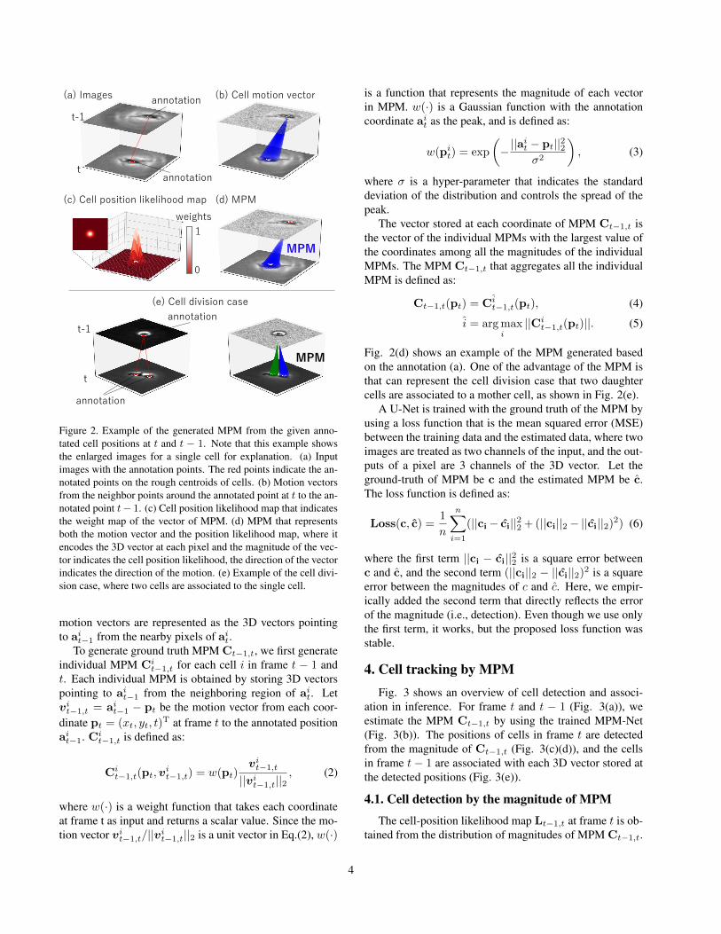
Figure 2. Example of the generated MPM from the given anno-tated cell positions at t and t − 1. Note that this example showsthe enlarged images for a single cell for explanation. (a) Inputimages with the annotation points. The red points indicate the an-notated points on the rough centroids of cells. (b) Motion vectorsfrom the neighbor points around the annotated point at t to the an-notated point t− 1. (c) Cell position likelihood map that indicatesthe weight map of the vector of MPM. (d) MPM that representsboth the motion vector and the position likelihood map, where itencodes the 3D vector at each pixel and the magnitude of the vec-tor indicates the cell position likelihood, the direction of the vectorindicates the direction of the motion. (e) Example of the cell divi-sion case, where two cells are associated to the single cell.

motion vectors are represented as the 3D vectors pointingto ait−1 from the nearby pixels of ait.

To generate ground truth MPM Ct−1,t, we first generateindividual MPM Ci

t−1,t for each cell i in frame t − 1 andt. Each individual MPM is obtained by storing 3D vectorspointing to ait−1 from the neighboring region of ait. Letvit−1,t = ait−1 − pt be the motion vector from each coor-

dinate pt = (xt, yt, t)T at frame t to the annotated position

ait−1. Cit−1,t is defined as:

Cit−1,t(pt,v

it−1,t) = w(pt)

vit−1,t

||vit−1,t||2

, (2)

where w(·) is a weight function that takes each coordinateat frame t as input and returns a scalar value. Since the mo-tion vector vi

t−1,t/||vit−1,t||2 is a unit vector in Eq.(2), w(·)

is a function that represents the magnitude of each vectorin MPM. w(·) is a Gaussian function with the annotationcoordinate ait as the peak, and is defined as:

w(pit) = exp

(−||a

it − pt||22σ2

), (3)

where σ is a hyper-parameter that indicates the standarddeviation of the distribution and controls the spread of thepeak.

The vector stored at each coordinate of MPM Ct−1,t isthe vector of the individual MPMs with the largest value ofthe coordinates among all the magnitudes of the individualMPMs. The MPM Ct−1,t that aggregates all the individualMPM is defined as:

Ct−1,t(pt) = Cit−1,t(pt), (4)

i = arg maxi

||Cit−1,t(pt)||. (5)

Fig. 2(d) shows an example of the MPM generated basedon the annotation (a). One of the advantage of the MPM isthat can represent the cell division case that two daughtercells are associated to a mother cell, as shown in Fig. 2(e).

A U-Net is trained with the ground truth of the MPM byusing a loss function that is the mean squared error (MSE)between the training data and the estimated data, where twoimages are treated as two channels of the input, and the out-puts of a pixel are 3 channels of the 3D vector. Let theground-truth of MPM be c and the estimated MPM be c.The loss function is defined as:

Loss(c, c) =1

n

n∑i=1

(||ci− ci||22 + (||ci||2− ||ci||2)2) (6)

where the first term ||ci − ci||22 is a square error betweenc and c, and the second term (||ci||2 − ||ci||2)2 is a squareerror between the magnitudes of c and c. Here, we empir-ically added the second term that directly reflects the errorof the magnitude (i.e., detection). Even though we use onlythe first term, it works, but the proposed loss function wasstable.

4. Cell tracking by MPMFig. 3 shows an overview of cell detection and associ-

ation in inference. For frame t and t − 1 (Fig. 3(a)), weestimate the MPM Ct−1,t by using the trained MPM-Net(Fig. 3(b)). The positions of cells in frame t are detectedfrom the magnitude of Ct−1,t (Fig. 3(c)(d)), and the cellsin frame t − 1 are associated with each 3D vector stored atthe detected positions (Fig. 3(e)).

4.1. Cell detection by the magnitude of MPM

The cell-position likelihood map Lt−1,t at frame t is ob-tained from the distribution of magnitudes of MPM Ct−1,t.

4

(b) MPM

MPM

t-1

t

frame t

frame t-1

(c) Cell positionlikelihood map

(a)Input Images

(e) Motion vectorsfrom detected cells

t-1

t

1

0

MPM-Net

(d) Detection results

Stretching each vector to t-1

Mapping magnitude of MPM

Figure 3. Overview of cell detection and association in inference.(a) Input images. (b) MPM estimated by MPM-Net. (c) Cell-position likelihood map determined from the magnitude of MPM.(d) The peaks are detected as cells at t. (e) The cell motion fromt to t− 1 is estimated by the direction vector at the detected peakpoint of MPM.

The detected cell positions are the coordinates of the eachlocal maximum of Lt−1,t. In the implementation, we ap-plied Gaussian smoothing as a pre-processing against noiseto Lt−1,t.

4.2. Cell association by MPM

The direction of each 3D vector of MPM Ct−1,t indi-cates the direction from position of the cell at t to position ofthe same cell at t−1. The position at frame t−1 is estimatedusing the triangle ratio from each vector of Ct−1,t stored ateach detected position in frame t, as shown in Fig. 4. Let thedetected position of each cell i be mi

t = (xit, yit, t)

T, andthe 3D vector stored in mi

t be vit−1,t = (∆x,∆y,∆t)T.

The estimated position mit−1 for each cell i at frame t − 1

is defined as:

mit−1 = (xit +

∆x

∆t, yit +

∆y

∆t, t− 1)T. (7)

We associate the detected cells in frame t with thetracked cells in frame t − 1 on the basis of mi

t−1 and theprevious confidence map Lt−2,t−1 used for the cell detec-tion in frame t − 1, as shown in Fig. 5. The estimatedposition mi

t−1 of cell i at t − 1 may be different from thetracked point at t − 1 which is located at a local maximumof cell-position likelihood map. Thus, we update the esti-mated position mi

t−1 to a certain local maximum that is theposition of a tracked cell Tj

i−1 by using the hill-climbingalgorithm to find the peak (the position of the tracked cell).Here, the j-th cell trajectory from sj until t − 1 is denotedas Tj = {Tj

sj , ...,Tjt−1}, where sj indicates the frame in

𝑥|𝑧=𝑡−1

𝑥|𝑧=𝑡

𝑧

𝒎𝑡𝑖

ෝ𝒎𝑡−1𝑖

Δ𝑡

Δ𝑥

1

Figure 4. Estimation of the cell position at frame t− 1

t-1 t t-1 t

𝒎𝒎𝑡𝑡𝑖𝑖

�𝒎𝒎𝑡𝑡−1𝑖𝑖

𝑻𝑻𝒕𝒕−𝟏𝟏𝒋𝒋

𝒎𝒎𝑡𝑡𝑘𝑘

𝒎𝒎𝑡𝑡𝑙𝑙

�𝒎𝒎𝒕𝒕−𝟏𝟏𝒌𝒌

�𝒎𝒎𝒕𝒕−𝟏𝟏𝒍𝒍

(a) Cell migration (one-to-one) (b) Cell division (one-to-two)

𝑻𝑻𝒕𝒕−𝟏𝟏𝒋𝒋

Figure 5. Illustration of association process. (a) The case of cellmigration (one-to-one matching): the estimated position mi

t−1 isassociated with the nearest tracked cell Tj

t−1. (b) The case ofcell division (one-to-two matching): two cells ml

t−1, mkt−1 are

associated as daughter cells of Tjt−1.

which the j-th cell trajectory started. If mit−1 was updated

to a position with Tji−1, we associate mi

t with Tjt−1 as the

tracked cell Tjt = mi

t. If the confidence value at the esti-mated position at t − 1 is zero (i.e., the point is not associ-ated with any cell), mi

t−1 is registered as a newly appearingcell TNt−1+1, whereNt−1 is the number of cell trajectoriesuntil time t before the update.

If two estimated cell positions mkt−1, ml

t−1 wereupdated to one tracked cell position Tj

t−1, these de-tected cells are registered as new born cells TN+1 ={mk

t−1}, TN+2 = {mlt−1}, i.e., daughter cells of Tj ,

and the division information is also registered Tj →TNt−1+1,TNt−1+2. The cell tracking method using MPMcan be performed very simply for both cell migration anddivision.

4.3. Interpolation for undetected cells

The estimated MPM at t may have a few false negativesbecause the estimation performance is not perfect. In thiscase, the trajectory Tj is not associated with any cell andthe frame-by-frame tracking for the cell is terminated at t−1for the moment. The tracklet Tj is registered as a temporar-ily track-terminated cell. During the tracking process usingMPM, if there are newly detected cells including daughtercells from cell division at t − 1 + q, the method tries to

5

12

timesp

ace

tt-1 t+1 t+2

Detected position

Motionvector

Cell division

Figure 6. Illustration of interpolation process for undetected cells.The newly detected cells (red) are associated with the track-terminated cells (green) using MPM.

associate the temporarily track-terminated cell using MPMagain, where the MPM is estimated by inputting the imagesat t− 1 and t− 1 + q (i.e., the time interval of the images isq). Next, the cell position is estimated and updated by us-ing frame-by-frame association. If the newly detected cellis associated with one of the temporarily track-terminatedcells, the cell is then associated with the cell and the posi-tions in the interval of frames, in which corresponding cellswere not detected, are interpolated based on the vector ofthe MPM. If there are multiple temporarily track-terminatedcells, this process is iterated on all track-terminated cells inascending order of time. The method excludes a cell fromthe list of the track-terminated cells when the interval fromthe endpoint of the track-terminated cell to the current frameis larger than a threshold. Here, we should note that cells att tend to be associated with another cell as cell divisionswhen a false negative occurs at t − 1. To avoid such false-positives of cell-division detection, the method tries to as-sociate such daughter cells with the track-terminated cells.This cell tracking algorithm can be performed online.

Fig. 6 shows an example of this process, in which thetracking of the green trajectory is terminated at t − 1 dueto false negatives at t, t + 1, and the red cell is detected att + 2. In this case, the MPM is estimated for three frameintervals (the inputs are the images at t− 1 and t+ 2), andit is associated with the track-terminated cell. Then, the cellpositions at t and t + 1 are interpolated using the vector ofMPM and the tracking starts again.

5. Experiments5.1. Data set

In the experiments, we used the open dataset [13] thatincludes time-lapse image sequences captured by phase-contrast microscopy since this is the same setup with ourtarget to track. In this data-set, the point-level ground truthis given, in which the rough cell centroid was annotatedwith cell ID, and hundreds of mouse myoblast stem cellswere cultured under four cell culture conditions that are dif-ferent growth-factor mediums; a) Control (no growth fac-tor), b) FGF2, c) BMP2, d) BMP2+FGF2, where there

18

Control (学習) FGF2

BMP2 (学習) FGF2+BMP2 (学習)*Dai Fei Elmer Ker+, “Phase contrast time-lapse microscopy datasets with automated and manual cell tracking annotations, ” Scientific Data, 2018, vol, 5.

(a) (b)

(c) (d)

(e)

(f)

(g)

(h)

Figure 7. Example images from four conditions. a) Control, b)FGF2, c) BMP2, d) BMP2+FGF2, (e)-(h) the enlarged images ofthe red box in (a)-(d), respectively. The appearance of cells are dif-ferent depending on the culture conditions. Cells often shrink andpartially overlapped in FGF2, cells tend to be spread under BMP2,there are both cells who are spread or shrunk under BMP2+FGF2.

are four image sequences for each condition (total: 16 se-quences). Since a stem cell is differentiated depending onthe growth factor, the cell appearance changes over the fourculture conditions as shown in Fig. 7.

The images were captured every 5 minutes and eachsequence consists of 780 images with the resolution of1392×1040 pixels. All cells were annotated in a sequencein BMP2, and three cells were randomly picked up at thebeginning of the sequence, and then the three cell’s familytrees through the 780-th image were annotated for all theother 15 sequences, where the number of the annotated cellsincreased with time due to cell division. The total numberof annotated cells in the 16 sequences is 135859 [21].

Since our method requires the training data that all cellsshould be fully annotated in each frame, we additionallyannotated cells in a part of frames under three conditions;Control: 100 frames, BMP2: 100 frames, FGF2+BMP2:200 frames. Totally the annotated 400 frames were used asthe training data, and the rest of the data was used as groundtruth in the test. To show the robustness for the cross-domain data (the different culture conditions from trainingdata) in the test, we did not make the annotation for FGF2.In all experiments, we set the interval value q for interpola-tion as 5.

5.2. Performance of cell Detection

The detection performance of our method compared withthe three other methods including the state-of-the-art; Ben-sch [4] that is based-on graph-cut, Bise [8] that is basedon physics model of phase-contrast microscopy [44], andHayashida [17] (the state-of-the-art for this data-set) that isbased on deep learning that estimates the cell-position like-lihood map that is similar to ours. Here, the annotation ofthis dataset is the point-level annotation, and thus we could

6

Figure 8. Examples of our cell detection results. Top: detectionresults. Green ’+’ indicates the true positive, red ’+’ indicatesthe false negative. Middle: cell position likelihood map generatedfrom the estimated MPM (Bottom).

not apply the learning-based segmentation methods that re-quire the pixel-level annotation for the individual cell re-gions. We used the fully-annotated sequence to measurethe precision, recall, and F1-score as the detection perfor-mance metrics. For the training and tuning the parameters,we used the same training sequences.

Fig. 8 shows examples of our cell detection results.Our method successfully detected the cells that have var-ious appearances, including spread cells, small brightercells, and touching cells. Table 1 shows the results of thecell detection evaluation. The deep learning-based meth-ods (Hayashida’s and ours) outperformed the other twomethods. The detection method in [17] estimated the cell-position likelihood map by U-net, in which their methodrepresents the detection but not for the association. Theterms of recall and F1-score of our method are slightly bet-ter (+1.4%) than those of their method. Since our methoduses the context from two successive frames in contrast totheir method that detects cells each frame independently,we consider that it would be possible to improve the perfor-mance of detection.

5.3. Performance of cell Tracking

Next, we evaluated the tracking performance of ourmethod with four other methods; Bensch [4] based-onframe-by-frame association with graph-cut segmentation;Chalfoun [10] based-on optimization for the frame-by-frame association with the segmentation results by [44];Bise[8] based on spatial-temporal global data association;Hayashida [17] based on motion flow estimation by CNN.Hayashida’s method is the most related to the proposedmethod. Their method estimates the cell position map andmotion flow by CNN, independently.

We used two quantitative criteria to assess the per-

Table 1. Cell detection performance on the terms of precision, re-call and F1-score.

MethodBensh

[4]Bise[8]

Hayashida[17] Ours

precision 0.583 0.850 0.968 0.964recall 0.623 0.811 0.902 0.932F1-score 0.602 0.830 0.934 0.948

Table 2. Association Accuracy.

Method Cont. FGF2 BMP2FGF2+BMP2 Ave.

Bensh[4] 0.604 0.499 0.801 0.689 0.648Chalfoun[10] 0.762 0.650 0.769 0.833 0.753Bise[8] 0.826 0.775 0.855 0.942 0.843Hayashida[17] 0.866 0.884 0.958 0.941 0.912Ours (MPM) 0.947 0.952 0.991 0.987 0.969

Table 3. Target Effectiveness.

Method Cont. FGF2 BMP2FGF2+BMP2 Ave.

Bensh[4] 0.543 0.448 0.621 0.465 0.519Chalfoun[10] 0.683 0.604 0.691 0.587 0.641*Li[23] 0.700 0.570 0.630 0.710 0.653*Kanade[21] 0.830 0.640 0.800 0.790 0.765Bise[8] 0.733 0.710 0.788 0.633 0.771Hayashida[17] 0.756 0.761 0.939 0.841 0.822Ours (MPM) 0.803 0.829 0.958 0.911 0.875

formance: association accuracy and target effectiveness[21]. To compute association accuracy, each target (human-annotated) was assigned to a track (computer-generated) foreach frame. The association accuracy was computed as thenumber of true positive associations divided by the numberof associations in the ground-truth. If a switch error oc-curred between two cells A and B, we count the two falsepositives (A→ B, B→ A). To compute target effectiveness,we first assign each target to a track that contains the mostobservations from that ground-truth. Then target effective-ness is computed as the number of the assigned track ob-servations over the total number of frames of the target.It indicates how many frames of targets are followed bycomputer-generated tracks. This metric is a stricter metric.If a switching error occurs in the middle of the trajectory,the target effectiveness is 0.5.

Table 2 and 3 show the performance of the associationaccuracy and the target effectiveness, respectively. In thesetables, the average scores for each condition (three or foursequences in each condition) are denoted 1. In Table 3, weshow the additional two methods as the reference; Li [23]

1The scores of the target effectiveness of *Li and *Kanade were eval-uated by the same data-set in their papers. Since the association accuracyof their methods [23, 21] were not described in their papers, we could notadd their performance at the Table 2.

7

Figure 9. Tracking results from each compared method underBMP2. (a) Bise, (b) Chalfoun, (c) Hayashida, (d) ours. Horizontalaxis indicate the time.

based on level-set tracking and Kande [21] based on frame-by-frame optimization. The performances of Bensh, Chal-foun, Li were sensitive depending on the culture condi-tions, and the performances were not good on both the met-ric terms, in particular, (FGF2) and (BMP2+FGF2). Weconsider that the sensitivity of their detection methods ad-versely affects the tracking performance. The methods ofBise and Kanade that use the same detection method [44]achieved better accuracy compared to the three methodsthanks to the better detection. The state-of-the-art method(Hayashida) furthermore improved the performances (Fig.9(c)) compared with the other current methods by esti-mating cell motion flow and position map independently.Our method (MPM) outperformed all the other methods(Fig. 9(d)). It improved +5.7% of association accuracy and+5.1% of the target-effectiveness on the average score com-pared to the second-best (Hayashida).

Fig. 10 shows the tracking results from ours under eachcondition, in which our method correctly tracked the vari-ous appearance of cells. Fig. 11 shows the tracking resultsin the case when a cell divided into two cells in the enlargedimage-sequence. Our method could correctly identify thecell division and track all cells in the region.

6. Conclusion

In this paper, we proposed the motion and position map(MPM) that jointly represents both detection and associa-tion, which can be represented in the cell division case notonly migration. The MPM encodes a 3D vector into eachpixel, where the distribution of magnitudes of the vectorsindicates the cell-position likelihood map, and the direc-tion of the vector indicates the motion direction from thepixel at t to the cell centroid at t − 1. Since MPM rep-resents both detection and association, it guarantees coher-

Figure 10. Tracking results from our method under each cultureconditions; (a) Control, (b) FGF2, (c) BMP2+FGF2. Althoughthe cell appearances are different depending on the conditions, ourmethod correctly tracked the cells.

Figure 11. Examples of our tracking results. (a) Entire image. (b)3D view of estimated cell trajectories. The z-axis indicates thetime, and each color indicates the trajectory of a single cell. (c) En-larged image sequence at the red box in (a), in which our methodcorrectly identified the cell division and tracked all cells.

ence; i.e., if a cell is detected, the association of the cellis always produced, and thus it improved the tracking per-formance. In the experiments, our method outperformedthe state-of-the-art method with over 5% improvement ofthe tracking performance under various conditions in realbiological images. In future work, we will develop an end-to-end tracking method that can estimate the entire cell tra-jectories from the entire sequence in order to use the globalspatial-temporal information on CNN.

Acknowledgments

This work was supported by JSPS KAKENHI GrantNumbers JP18H05104 and JP18H04738.

8

References[1] Saad Ullah Akram, Juho Kannala, Lauri Eklund, and Janne

Heikkila. Joint cell segmentation and tracking using cell pro-posals. In Proceedings of the IEEE International Symposiumon Biomedical Imaging (ISBI), pages 920–924, 2016.

[2] Sadeghian Amir, Alahi Alexandre, and Savarese Silvio.Tracking the untrackable: Learning to track multiple cueswith long-term dependencies. In Proceedings of the IEEEInternational Conference on Computer Vision (ICCV), pages300–311, 2017.

[3] Assaf Arbelle and Tammy Riklin Raviv. Microscopy cellsegmentation via convolutional lstm networks. In Proceed-ings of the IEEE International Symposium on BiomedicalImaging (ISBI), pages 1008–1012, 2019.

[4] Robert Bensch and Olaf Ronneberger. Cell segmentationand tracking in phase contrast images using graph cut withasymmetric boundary costs. In Proceedings of the IEEE In-ternational Symposium on Biomedical Imaging (ISBI), pages1220–1223, 2015.

[5] Ryoma Bise, Kang Li, Sungeun Eom, and Takeo Kanade.Reliably tracking partially overlapping neural stem cells indic microscopy image sequences. In International Confer-ence on Medical Image Computing and Computer-AssistedIntervention Workshop (MICCAIW), pages 67–77, 2009.

[6] Ryoma Bise, Yoshitaka Maeda, Mee-hae Kim, and MasahiroKino-oka. Cell tracking under high confluency conditions bycandidate cell region detection-based-association approach.In Proceedings of Biomedical Engineering, pages 1004–1010, 2011.

[7] Ryoma Bise and Yoichi Sato. Cell detection from redundantcandidate regions under non-overlapping constraints. IEEETrans. on Medical Imaging, 34(7):1417–1427, 2015.

[8] Ryoma Bise, Zhaozheng Yin, and Takeo Kanade. Reliablecell tracking by global data association. In Proceedings ofthe IEEE International Symposium on Biomedical Imaging(ISBI), pages 1004–1010, 2011.

[9] Doersch Carl and Zisserman Andrew. Multi-task selfsuper-vised visual learning. In Proceedings of the IEEE Interna-tional Conference on Computer Vision (ICCV), 2017.

[10] Joe Chalfoun, Michael Majurski, Alden Dima, Michael Hal-ter, Kiran Bhadriraju, and Mary Brady. Lineage mapper: Aversatile cell and particle tracker. Scientific reports, 6:36984,2016.

[11] Eigen David and Fergus Rob. Predicting depth, surface nor-mals and semantic labels with a common multi-scale convo-lutional architecture. In Proceedings of the IEEE Interna-tional Conference on Computer Vision(ICCV), pages 3994–4003, 2015.

[12] Zhao Dawei, Fu Hao, Xiao Liang, Wu Tao, and Dai Bin.Multi-object tracking with correlation filter for autonomousvehicle. Sensors.

[13] Ker Elmer D.F., Sho Sanami Seunguen, Eom, and RyomaBise et al. Phase contrast time-lapse microscopy datasetswith automated and manual cell tracking annotations. Scien-tific Data, 2018.

[14] Yu Fengwei, Li Wenbo, Li Quanquan, Liu Yu, Shi Xiaohua,and Yan Junjie. Multiple object tracking with high perfor-

mance detection and appearance feature. In European Con-ference on Computer Vision (ECCV), pages 36–42, 2016.

[15] Jan Funke, Lisa Mais, Andrew Champion, Natalie Dye, andDagmar Kainmueller. A benchmark for epithelial cell track-ing. In Proceedings of The European Conference on Com-puter Vision (ECCV) Workshops, 2018.

[16] Gkioxari Georgia, Hariharan Bharath, Girshick Ross, andMalik Jitendra. R-cnns for pose estimation and action de-tection. In arXive, 2014.

[17] Junya Hayashida and Ryoma Bise. Cell tracking with deeplearning for cell detection and motion estimation in low-frame-rate. In International Conference on Medical ImageComputing and Computer-Assisted Intervention (MICCAI),pages 397–405, 2019.

[18] Kokkinos Iasonas. Ubernet: Training a universal convolu-tional neural network for low-, mid-, and high-level visionusing diverse datasets and limited memory. In Proceedingsof the IEEE Conference on Computer Vision and PatternRecognition (CVPR), 2017.

[19] Misra Ishan, Shrivastava Abhinav, Gupta Abhinav, andHebert Martial. Cross-stitch networks for multi-task learn-ing. In Proceedings of the IEEE Conference on ComputerVision and Pattern Recognition (CVPR), pages 3994–4003,2016.

[20] Valmadre Jack, Bertinetto Luca, Henriques Joao, VedaldiAndrea, and Torr Philip H.S. End-to-end representationlearning for correlation filter based tracking. In Proceed-ings of the IEEE Conference on Computer Vision and PatternRecognition (CVPR), pages 2805–2813, 2017.

[21] Takeo Kanade, Zhaozheng Yin, Ryoma Bise, Seungil Huh,Sungeun Eom, Michael F. Sandbothe, and Mei Chen. Cellimage analysis: Algorithms, system and applications. InProceedings of the IEEE Winter Conference on Applicationsof Computer Vision (WACV). IEEE, 2011.

[22] Bo Li, Wei Wu, Zheng Zhu, and Junjie Yan. High perfor-mance visual tracking with siamese region proposal network.In Proceedings of the IEEE Conference on Computer Visionand Pattern Recognition (CVPR), 2018.

[23] Kang Li and Takeo Kanade. Nonnegative mixed-norm pre-conditioning for microscopy image segmentation. In In-ternational Conference Information Processing in MedicalImaging (IPMI), pages 362–373, 2009.

[24] Kang Li, Eric D Miller, Mei Chen, Takeo Kanade, Lee EWeiss, and Phil G Campbell. Cell population tracking andlineage construction with spatiotemporal context. Medicalimage analysis, 12(5):546–566, 2008.

[25] Min Liu, Ram Kishor Yadav, Amit Roy-Chowdhury, andG Venugopala Reddy. Automated tracking of stem cell lin-eages of arabidopsis shoot apex using local graph matching.The Plant Journal, 62(1):135–147, 2010.

[26] Wang Lu, Xu Lisheng, Kim Min-Young, Luca Rigazico, andYang Ming-Hsuan. Online multiple object tracking via flowand convolutional features. In Proceedings of the IEEE In-ternational Conference on Image Processing (ICIP), pages3630–3634, 2017.

[27] Filip Lux and Petr Matula. Dic image segmentation of densecell populations by combining deep learning and watershed.

9

In Proceedings of the IEEE International Symposium onBiomedical Imaging (ISBI), pages 236–239, 2019.

[28] Katya Mkrtchyan, Damanpreet Singh, Min Liu, V Reddy, ARoy-Chowdhury, and M Gopi. Efficient cell segmentationand tracking of developing plant meristem. In IEEE Interna-tional Conference on Image Processing(ICIP), pages 2165–2168, 2011.

[29] Kazuya Nishimura, Ryoma Bise, et al. Weakly supervisedcell instance segmentation by propagating from detection re-sponse. In International Conference on Medical Image Com-puting and Computer-Assisted Intervention (MICCAI), pages649–657. Springer, 2019.

[30] Kenji Okuma, Ali Taleghani, Nando De Freitas, James J Lit-tle, and David G Lowe. A boosted particle filter: Multitargetdetection and tracking. In European conference on computervision(ECCV), pages 28–39, 2004.

[31] Al-Kofahi Omar, Radke Richard, Goderie Susan, Shen Qin,Temple Sally, and Badrinath Roysam. Automated cell lin-eage construction: A rapid method to analyze clonal devel-opment established with murine neural progenitor cells.

[32] Christian Payer, Darko Stern, Thomas Neff, Horst Bischof,and Martin Urschler. Instance segmentation and trackingwith cosine embeddings and recurrent hourglass networks.In International Conference on Medical Image Computingand Computer-Assisted Intervention (MICCAI), pages 3–11,2018.

[33] Markus Rempfler, Sanjeev Kumar, Valentin Stierle, PhilippPaulitschke, Bjoern Andres, and Bjoern H Menze. Cell lin-eage tracing in lens-free microscopy videos. In InternationalConference on Medical Image Computing and Computer-Assisted Intervention (MICCAI), pages 3–11, 2017.

[34] Markus Rempfler, Valentin Stierle, Konstantin Ditzel, San-jeev Kumar, Philipp Paulitschke, Bjoern Andres, and Bjo-ern H Menze. Tracing cell lineages in videos of lens-freemicroscopy. Medical image analysis, 48:147–161, 2018.

[35] Henschel Roberto, Marcard Timo von, and Rosenhahn Bodo.Simultaneous identification and tracking of multiple peopleusing video and imus. In Proceedings of the IEEE ComputerVision and Pattern Recognition Workshop (CVPRW), 2019.

[36] Martin Schiegg, Philipp Hanslovsky, Bernhard X Kausler,Lars Hufnagel, and Fred A Hamprecht. Conservation track-ing. In Proceedings of the IEEE International Conference onComputer Vision(ICCV), pages 2928–2935, 2013.

[37] Sun ShiJie, Akhtar Naveed, Song HuanSheng, MianS.Ajmal, and Shah Mubarak. Deep affinity network for mul-tiple object tracking. IEEE Transactions on Pattern Analysisand Machine Intelligence.

[38] Ihor Smal, Wiro Niessen, and Erik Meijering. Bayesiantracking for fluorescence microscopic imaging. In Proceed-ings of the IEEE International Symposium on BiomedicalImaging (ISBI), pages 550–553, 2006.

[39] Hang Su, Zhaozheng Yin, Seungil Huh, and Takeo Kanade.Cell segmentation in phase contrast microscopy images viasemi-supervised classification over optics-related features.Medical image analysis, 17(7):746–765, 2013.

[40] Xiaoxu Wang, Weijun He, Dimitris Metaxas, Robin Mathew,and Eileen White. Cell segmentation and tracking using

texture-adaptive snakes. In Proceedings of the IEEE Inter-national Symposium on Biomedical Imaging (ISBI), pages101–104, 2007.

[41] Xiao Wen, Vallet Bruno, Schindler Konrad, and PaparoditisNicolas. Simultaneous detection and tracking of pedstrianfrom panoramic laser scanning data. In ISPRS Annals of thePhotogrammetry, Remote Sensing and Spatial InformationSciences, 2016.

[42] Zheng Wu, Danna Gurari, Joyce Wong, and Margrit Betke.Hierarchical partial matching and segmentation of interact-ing cells. In Proceedings of the International Conference onMedical Image Computing and Computer-Assisted Interven-tion (MICCAI), pages 389–396, 2012.

[43] Fuxing Yang, Michael A Mackey, Fiorenza Ianzini, GregGallardo, and Milan Sonka. Cell segmentation, tracking, andmitosis detection using temporal context. In InternationalConference on Medical Image Computing and Computer-Assisted Intervention (MICCAI), pages 302–309, 2005.

[44] Zhaozheng Yin, Takeo Kanade, and Mei Chen. Under-standing the phase contrast optics to restore artifact-free mi-croscopy images for segmentation. Medical image analysis,16(5):1047–1062, 2012.

[45] Zeng Zhiliang, Xianzhi Li, Kin Ying, and Fu Yu Chi-Wing.Deep floor plan rproceedings of theecognition using a multi-task network with room-boundary-guided attention. In Pro-ceedings of the IEEE International Conference on ComputerVision (ICCV), pages 9096–9104, 2019.

[46] Zibin Zhou, Fei Wang, Wenjuan Xi, Huaying Chen, PengGao, and Chengkang He. Joint multi-frame detection andsegmentation for multi-cell tracking. International Confer-ence on Image and Graphics (ICIG), 2019.

10