MPC Performance Tuning

ECE5590: Model Predictive Control 7–1

MPC Performance Tuning

! MPC algorithms incorporate a number of adjustable designparameters that give enormous flexibility to the configuration of thecontrol system

! By delivering all this flexibility, they can also complicate the task ofcontroller tuning

! Among the degrees of freedom one can deploy in order to achievekey control objectives in MPC are the following:

– Horizons, Np, Nc

– Weights, Q, R

– Observer dynamics

– Reference trajectory

– Disturbance model

! The notion of tuning in MPC refers to the systematic adjustment ofproblem degrees of freedom with a view toward achieving desiredperformance outcomes

! Before addressing specific tuning guidelines, et’s first review somekey ideas related to stability and performance for control systems

Lecture notes prepared by M. Scott Trimboli. Copyright c" 2010-2015, M. Scott Trimboli

ECE5590, MPC Performance Tuning 7–2

The role of feedback

Feedback is used to overcome the effects of uncertainty

Feedback is dangerous

! It is well-known that introducing feedback brings with it the possibilityof destabilizing a stable system

! If the system model and environment are known perfectly, thenperfect control can be achieved using an open-loop control strategy

! But feedback can be very effective for reducing effects ofdisturbances and model uncertainty

– If our only objective was to follow a set-point well, then we don’tneed feedback - open-loop works fine!

! But we can deduce other information from set-point responses, so it’snot pointless to use them

Two-degree-of-freedom system

F (z) K(z)

H(z)

P (z)s r e u

d

n

y

+−

+

+

+

+Controller

Plant



! In the two-degree-of-freedom system, set-point s is filtered by apre-filter F.z/ before becoming reference r

! Controller has two parts: i) forward path controller K.z/; and ii)feedback path controller H.z/

! Output disturbance d and measurement noise n are also present

! We need to find transfer functions relating input signals s, d , and n, tooutput signals y and u

! For the general (vector-valued) case,

y.z/ D d.z/ C P.z/K.z/e.z/

e.z/ D F.z/s.z/ # H.z/ Œn.z/ C y.z/!

! This givesy.z/ D d.z/ C P.z/K.z/ fF.z/s.z/ # H.z/ Œn.z/ C y.z/!g

andŒI C P.z/K.z/H.z/! y.z/ D

d.z/ C P.z/K.z/F.z/s.z/ # P.z/K.z/H.z/n.z/

! We can express this result asy.z/ D S.z/d.z/ C S.z/P.z/K.z/F.z/s.z/ # T .z/n.z/

where we define the sensitivity function S.z/ and the complementarysensitivity function T .z/ as

S.z/ D ŒI C P.z/K.z/H.z/!#1

T .z/ D ŒI C P.z/K.z/H.z/!#1 P.z/K.z/H.z/



! In feedback theory, the smaller the sensitivity, the better the feedback,i.e., effect of d is kept small

! Likewise, the smaller the complementary sensitivity, the smaller theeffect of measurement noise n

! Note alsoS.z/ C T .z/ D I

which means you can’t have S.z/ and T .z/ small (near zero)simultaneously

! Note that the response of the output to the set-point can be designedindependantly via the pre-filter F.z/

! The MPC control problem considers tracking a reference subject toconstraints

– Although this looks straighforward mathematically in the algorithm,it’s not necessarily related to good feedback properties

– It is especially challenging to consider the effect of feedbackproperties under constraints - few analytical tools exist

Special Cases

! Here we consider some special choices of parameters and deducehow the predictive controller will behave

Mean-level control

! Choose Nc D 1 and R D 0.

! The cost function can be written,



J.k/ DNpXiD1

k Oy.k C i jk/ # rk2Q

! Since here we can only untilize one control move, 4u.k/, then ifNp ! 1, the optimal strategy is to move the control to that levelwhich will give y D r in the steady-state

! In this case, the transient response of the system will be theopen-loop response of the plant

! This is a common configuration for feedback systems; it also gives usa compatible form with which to describe the unconstrained modelpredictive controller formulation developed previously and shownbelow

Deadbeat control

! Let Nc D n , the number of states in the plant

! Assume R D 0; assume r.k C i/ D r , and choose Np $ 2n

! The cost function is then,

J.k/ D2nX

iDn

k Oy.k C i jk/ # rk2Q

’Perfect’ control

! Choose Np D 1 and Nc D 1 with R D 0

! The cost function is then,

J.k/ D k Oy.k C 1jk/ # r.k C 1/k2Q



! An optimal strategy in this case is to choose input signals so that thenext output matches the input reference as closely as possible. Thereis no concern about future steps.

! Consider the SISO transfer function case,

Y.z/ D G.z/U.z/ D B.z/

A.z/U.z/

! Writing as a difference equation,b0u.k/ D y.k C 1/ C : : : C any.k C 1 # n/ # b1u.k # 1/ # : : : # bnu.k # n/

! We can choose u.k/ such as to make y.k C 1/ D r.k C 1/ by settingb0u.k/ D r.kC1/Ca1y.k/C: : :Cany.kC1#n/#b1u.k#1/#: : :#bnu.k#n/

! If this is done at each step, we will eventually have

y.k/ D r.k/

y.k # 1/ D r.k # 1/

so that,b0u.k/ D r.kC1/Ca1r.k/C: : :Canr.kC1#n/#b1u.k#1/#: : :#bnu.k#n/

orB.z#1/u.k/ D A.z#1/r.k C 1/

! So, what we essentially have is a controller that is the inverse of theplant.

Example 7.1

! It will be instructive to examine an example to develop insight into theeffect various tuning parameters have on stability and performance

! Consider the system described by (Rossiter, Ch. 5.2)



Y.z/ D z#1 C 0:2z#2

.1 # 0:9z#1/.1 # 0:8z#1/U.z/

G.z/ D z#1 C 0:2z#2

1 # 1:7z#1 C 0:72z#2

D z C 0:2

z2 # 1:7z C 0:72

– The state space representation is

xm.k C 1/ D"

1:7 #0:72

1 0

#xm.k/ C

"1

0

#u.k/

y.k/ Dh

1 0:2i

xm.k/ C Œ0! u.k/

! Writing the augmented state vector,

x.k/ D"

4xm.k/

y.k/

#

– The state equations become

x.k C 1/ D"

4xm.k/

y.k/

#D

"Am 0t

m

CmAm 1

# "4xm.k/

y.k/

#

C"

Bm

CmBm

#4u.k/

y.k/ Dh

0m 1i "

4xm.k/

y.k/

#

which for our example this gives



A D

264

1:7 #0:72 0

1 0 0

1:9 #0:72 1

375 B D

264

1

0

1

375

C Dh

0 0 1i

! Note that the eigenvalues of A are ".A/ Dn

1:0 0:9 0:8o

.

! Using this example, we can systematically vary the parameters andexamine the effect on output response and control input.

! First we’ll examine the case where Nc D 1 and vary the predictionhorizon. The following plots depict the output, control input andcontrol input increment as functions of varying the prediction horizon.

0 5 10 15 20 250

0.2

0.4

0.6

0.8

1

1.2

1.4

1.6

Sampling Instant

y[k]

Example 7.1 Np=1,2,3,5,10,20 Nc=1, R=1

Np=1Np=2Np=3Np=5Np=10Np=20



5 10 15 20 25−1

−0.8

−0.6

−0.4

−0.2

0

0.2

0.4

0.6

0.8

1

Sampling Instant

u[k]

Example 7.1 Np=1,2,3,5,10,20 Nc=1, R=1


5 10 15 20 25−1

−0.8

−0.6

−0.4

−0.2

0

0.2

0.4

0.6

0.8

1

Sampling Instant

delu

[k]

Example 7.1 Np=1,2,3,5,10,20 Nc=1, R=1


! Next, we’ll fix the prediction horizon at Np D 20 and vary the controlhorizon. Resulting plots follow.



5 10 15 20 250

0.2

0.4

0.6

0.8

1

1.2

1.4

1.6

Sampling Instant

y[k]

Example 7.1 Np=20, Nc=1,2,3,5,10,20, R=1

Nc=1Nc=2Nc=3Nc=5Nc=10Nc=20

5 10 15 20 25−1

−0.8

−0.6

−0.4

−0.2

0

0.2

0.4

0.6

0.8

1

Sampling Instant

u[k]

Example 7.1 Np=20, Nc=1,2,3,5,10,20, R=1




5 10 15 20 25−1

−0.8

−0.6

−0.4

−0.2

0

0.2

0.4

0.6

0.8

1

Sampling Instant

delu

[k]

Example 7.1 Np=20 Nc=1,2,3,5,10,20 R=1


! It appears from these plots that qualitative improvements in systemresponse are achieved for increasing values of the control horizon

! Setting the prediction horizon to a smaller value (Np D 3) gives thefollowing results.

0 5 10 15 20 250

0.2

0.4

0.6

0.8

1

1.2

1.4

Sampling Instant

y[k]

Example 7.1 Np=3 Nc=1,2,3 R=1

Nc=1Nc=2Nc=3



5 10 15 20 25−1

−0.8

−0.6

−0.4

−0.2

0

0.2

0.4

0.6

0.8

1

Sampling Instant

u[k]


Nc=1Nc=2Nc=3

5 10 15 20 25−1

−0.8

−0.6

−0.4

−0.2

0

0.2

0.4

0.6

0.8

1

Sampling Instant

delu

[k]


Nc=1Nc=2Nc=3

! Clearly, increasing Nc improves the response for small values of Np

! For comparison, we plot the deadbeat response (achieved by settingR D 0)



0 5 10 15 20 250

0.2

0.4

0.6

0.8

1

1.2

1.4

y[k]

Sampling Instant

Example 7.1 Deadbeat Control

! Now we’ll set Np D 10, Nc D 3 and vary the control incrementweighting

5 10 15 20 250

0.2

0.4

0.6

0.8

1

1.2

1.4

1.6

Sampling instant

y[k]

Example 7.1 Np=10 Nc=3 R=0.01, 0.1, 1, 10, 100

R=0.01R=0.1R=1R=10R=100



5 10 15 20 25−1

−0.8

−0.6

−0.4

−0.2

0

0.2

0.4

0.6

0.8

1

Sampiing Instant

u[k]

Example 7.1 Np=10 Nc=3 R=0.01, 0.1, 1, 10, 100

R=0.01R=0.1R=1R=10R=100

0 5 10 15 20 25−2

−1.5

−1

−0.5

0

0.5

1

Sampling Instant

delu

[k]

Example 7.1 Np=10 Nc=3 R=0.01, 0.1, 1, 10, 100

R=0.01R=0.1R=1R=10R=100

! It is apparent that lower values of control increment weighting allowlarger excursions in the control signal and bring about a fasterresponse



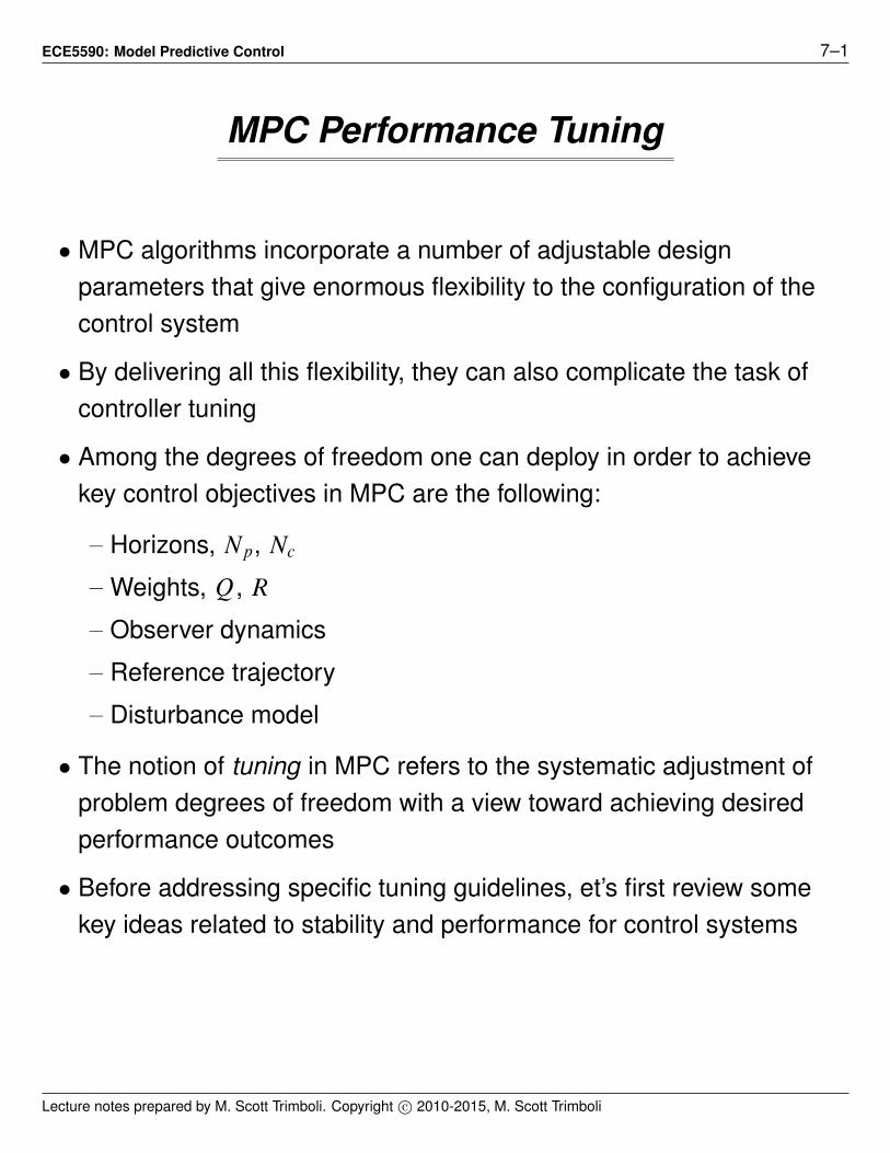
! Let’s now see if we can force “perfect” control by setting Np D Nc D 1

and R D 0. Results appear below.

0 5 10 15 20 250

0.2

0.4

0.6

0.8

1

1.2

1.4

Sampling Instant

y[k]

Example 7.1 "Perfect" Control

0 5 10 15 20 25−1

−0.8

−0.6

−0.4

−0.2

0

0.2

0.4

0.6

0.8

1

Sampling Instant

u[k]




0 5 10 15 20 25−2

−1.5

−1

−0.5

0

0.5

1

1.5

delu

[k]

Sampling Instant


! It looks like we’ve achieved the output objective in a single time step

– We can verify this result by solving the simultaneous set ofdifference equations

yŒk! D 1:7yŒk # 1! # 0:72yŒk # 2! C uŒk # 1! C 0:2uŒk # 2!

yŒ1! D 1:7 % yŒ0! # 0:72 % 0 C uŒ0! C 0:2 % 0 D 1

yŒ2! D 1:7 % yŒ1! # 0:72 % yŒ0! C uŒ1! C 0:2 % uŒ0! D 1

yŒ3! D 1:7 % yŒ2! # 0:72 % yŒ1! C uŒ2! C 0:2 % uŒ1! D 1::: ::: :::

– Note that this works here since G.z/ is proper (but not strictlyproper)

! Let’s state some general observations:

– If Nc is small, then increasing Np results in slower loop dynamics(approaches open-loop)

– If Nc is large, then increasing Np improves performance



– If Np is small, then increasing Nc can lead to near deadbeatbehavior

– Increasing control weighting R slows down the response

– Decreasing control weighting R speed up the response

! How do we choose horizons?

! Some guidelines:

– As Np is increased, nominal closed-loop performance improves ifNc is large enough

– As Nc is increased, nominal closed-loop performance improves ifNp is large enough

! For a well-posed optimization, Nc should be large and Np # Nc shouldbe greater than the system settling time

! How do we choose control weighting?

! Some guidelines:

– Greater control weighting generally means less active inputchanges

– Increasing weights indefinitely reduces control activity to zero -switching off feedback

– For large prediction horizons, it is possible to out-weigh controlwith error magnitude measure

! Considerations for open-loop unstable plants

– Large Np values in standard MPC design may cause performancedegradation for open-loop unstable plants



– Large Np values can cause ill-conditioning of the numericalcomputations for open-loop unstable plants

! In general (but not always) it is difficult to obtain acceptableperformance for Nc D 1

Systematic tuning strategies

! It is often tempting to pursue strategies that seek to ’optimize’ outputperformance in some meaningful way

! One example of this might be to measure the output error for varioustuning parameters and compare results

! For the following study, the system of Example 7.1 was used and thesum-of-squares of the output error for Np D 20 was computed andcompared for values of Nc D 1; 2; 3; 5; 10 and 20:

1 1.5 2 2.5 3 3.5 4 4.5 5 5.5 61

2

3

4

5

6

7

Nc Index

Squa

red

Out

put E

rror

Parametric Study: Nc

! A clear improvement is seen in moving from Nc D 1 to Nc D 2 . Onlymarginal improvements are seen with further increases in Nc.



! The next study compares the same error criterion for Nc D 1 anddifferent values of Np.

1 1.5 2 2.5 3 3.5 4 4.5 5 5.5 61

2

3

4

5

6

7

Np Index

Squa

red

Out

put E

rror

Example 7.1 Parametric Analysis: Np

! This result shows a rather clear minimum for Np D 2


(mostly blank)

Documents

MPC Performance Tuning